basu’s theorem with applications: a ...sankhya.isical.ac.in/search/64a3/64a3032.pdfbasu’s...

Sankhya : The Indian Journal of Statistics

Special issue in memory of D. Basu

2002, Volume 64, Series A, Pt. 3, pp 509-531

BASU’S THEOREM WITH APPLICATIONS:A PERSONALISTIC REVIEW

By MALAY GHOSHUniversity of Florida, Florida, USA

SUMMARY. The paper revisits Basu’s Theorem, and documents some of its many

applications in statistical inference. There is also some discussion on the relationship

between the concepts of sufficiency, completeness and ancillarity.

1. IntroductionThere are not many simple results in statistics whose popularity has

stood the test of time. Basu’s Theorem is a clear exception. The result notonly remains popular nearly fifty years after its discovery, but the zest andenthusiasm about the theorem that was evidenced in the fifties and sixtieshas not diminished with the passage of time. Indeed, the theorem makeseminent appearance in advanced texts such as Lehmann (1986) and Lehmannand Casella (1998) as well as intermediate texts such as Mukhopadhyay(2000) and Casella and Berger (2001).

At first sight, Basu’s Theorem appears as a purely technical result, and itis possibly the technical aspect of the theorem that has led to its many diverseapplications. But the result also has its conceptual merits. As pointed outby Basu (1982) himself, the theorem shows connection between sufficiency,ancillarity and independence, concepts that were previously perceived asunrelated, and has subsequently led to deeper understanding of the interre-lationship between these concepts.

I first came across Basu’s Theorem in my Ph.D. inference course inChapel Hill. I was immediately struck by the sheer elegance of the re-sult, though, admittedly at that point, I did not see its full potentiality forapplications.

Paper received December 2001.

AMS (2000) subject classification. 62B05, 62A01.

Keywords and phrases. Sufficiency, completeness, ancillarity, empirical Bayes, infinite di-

visibility.

510 malay ghosh

Over the years, while teaching inference courses for graduate students, Icould realize more and more the utility of the result. The theorem is not justuseful for what it says, it can be used in a wide range of applications such asin distribution theory, hypothesis testing, theory of estimation, calculationof ratios of moments of many complicated statistics, calculation of meansquared errors of empirical Bayes estimators, and even surprisingly, estab-lishing infinite divisibility of certain distributions. The application possiblyextends to many other areas of statistics which I have not come across.

What I attempt in this article is a personalistic review of Basu’s Theoremand many of its applications. The review is, by no means, comprehensiveand has possibly left out many important contributions by different authors.For this, I offer my sincerest apology at the outset.

The outline of the remaining sections is as follows. Section 2 introducesBasu’s Theorem and its implications. This section also discusses possibleconverses of this theorem (Koehn and Thomas, 1975; Lehmann, 1981). Sec-tion 3 discusses some immediate simple applications of Basu’s Theorem indistribution theory as well as in some moment calculations. Section 4 dis-cusses applications in classical hypothesis testing. Section 5 shows some usesin finding uniformly minimum variance unbiased estimators (UMVUE’s) andbest equivariant estimators. Section 6 contains applications in the calcula-tion of mean squared errors of empirical Bayes estimators. Finally, Section 7shows its use in proving some infinite divisibility theorems. Those interestedonly in applications of the theorem may skip the remainder of Section 2 afterTheorem 1, and proceed straight to Section 3.

While writing this review article, I have benefitted considerably by Basu’s(1982) own writing on the topic in the Encyclopedia of Statistical Sciences,the illuminating article of Lehmann (1981), and the very elegant contribu-tion of Boos and Hughes-Oliver (1998) which deals with many interestingapplications, some of which are repeated in this paper. I enjoyed readingmany other interesting contributions, too numerous to mention each oneindividually.

2. Basu’s Theorem and its Role in Statistical Inference

Consider a random variable X on some measurable space X . Typically,X = Rn, the n-dimensional Euclidean space for some n. The distributionof X is indexed by θ ∈ Θ. Let P = {Pθ : θ ∈ Θ} denote the family ofdistributions of X. A statistic T ≡ T (X) is said to be sufficient for θ,(or more appropriately for the family P) if the conditional distribution of

basu’s theorem with applications 511

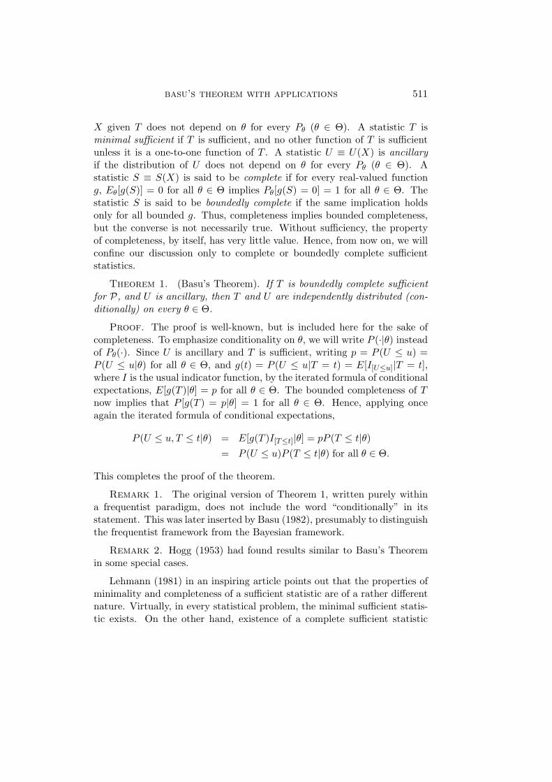
X given T does not depend on θ for every Pθ (θ ∈ Θ). A statistic T isminimal sufficient if T is sufficient, and no other function of T is sufficientunless it is a one-to-one function of T . A statistic U ≡ U(X) is ancillaryif the distribution of U does not depend on θ for every Pθ (θ ∈ Θ). Astatistic S ≡ S(X) is said to be complete if for every real-valued functiong, Eθ[g(S)] = 0 for all θ ∈ Θ implies Pθ[g(S) = 0] = 1 for all θ ∈ Θ. Thestatistic S is said to be boundedly complete if the same implication holdsonly for all bounded g. Thus, completeness implies bounded completeness,but the converse is not necessarily true. Without sufficiency, the propertyof completeness, by itself, has very little value. Hence, from now on, we willconfine our discussion only to complete or boundedly complete sufficientstatistics.

Theorem 1. (Basu’s Theorem). If T is boundedly complete sufficientfor P, and U is ancillary, then T and U are independently distributed (con-ditionally) on every θ ∈ Θ.

Proof. The proof is well-known, but is included here for the sake ofcompleteness. To emphasize conditionality on θ, we will write P (·|θ) insteadof Pθ(·). Since U is ancillary and T is sufficient, writing p = P (U ≤ u) =P (U ≤ u|θ) for all θ ∈ Θ, and g(t) = P (U ≤ u|T = t) = E[I[U≤u]|T = t],where I is the usual indicator function, by the iterated formula of conditionalexpectations, E[g(T )|θ] = p for all θ ∈ Θ. The bounded completeness of Tnow implies that P [g(T ) = p|θ] = 1 for all θ ∈ Θ. Hence, applying onceagain the iterated formula of conditional expectations,

P (U ≤ u, T ≤ t|θ) = E[g(T )I[T≤t]|θ] = pP (T ≤ t|θ)= P (U ≤ u)P (T ≤ t|θ) for all θ ∈ Θ.

This completes the proof of the theorem.

Remark 1. The original version of Theorem 1, written purely withina frequentist paradigm, does not include the word “conditionally” in itsstatement. This was later inserted by Basu (1982), presumably to distinguishthe frequentist framework from the Bayesian framework.

Remark 2. Hogg (1953) had found results similar to Basu’s Theoremin some special cases.

Lehmann (1981) in an inspiring article points out that the properties ofminimality and completeness of a sufficient statistic are of a rather differentnature. Virtually, in every statistical problem, the minimal sufficient statis-tic exists. On the other hand, existence of a complete sufficient statistic

512 malay ghosh

implies the existence of a minimal sufficient statistic (Bahadur, 1957). Aspointed out by Lehmann (see also Boos and Hughes-Oliver, 1998), existenceof a minimal sufficient statistic, by itself, does not guarantee that there doesnot exist any function of T which is ancillary. Basu’s Theorem tells us thatif T is complete in addition to being sufficient, then no ancillary statisticother than the constants can be computed from T . Thus, by Basu’s Theo-rem, completeness of a sufficient statistic T characterizes the success of T inseparating the informative part of the data from that part, which by itself,carries no information.

The above point is well-illustrated by the following example (see Lehmann,1981).

Example 1. Let X1, · · · , Xn be independent and identically distributed(iid) with joint probability density function (pdf) belonging to the logisticfamily

P =

{n∏

i=1

fθ(xi) : fθ(x) = f(x − θ), x ∈ R1, θ ∈ R1

}, (2.1)

where f(x) = exp(x)/[1 + exp(x)]2. Let X(1) ≤ X(2) ≤ · · · ≤ X(n) denotethe ordered Xi’s. It is well-known (see e.g. Lehmann and Casella, 1998,p.36) that T = (X(1), · · · , X(n)) is minimal sufficient for P. But clearly Tis not boundedly complete as can be verified directly by showing that theexpectation of any bounded function of X(n) − X(1) (with the exception ofconstants) is a nonzero constant not depending on θ, but that the probabilitythat the function is equal to that constant is not 1 (in fact equal to zero).Alternately, one may note that X(n)−X(1) is ancillary, and is not independentof T . On the other hand, if one considers instead the augmented class ofall continuous pdf’s P = {∏n

i=1 f(xi) : f continuous}, then T is indeedcomplete (see Lehmann, 1986, pp 143-144), and Basu’s Theorem assertsthat there does not exist any non-constant function of T which is ancillary.

Hence, as pointed out by Lehmann (1981), for the logistic family, (he pro-duces other examples as well), sufficiency has not been successful in “squeez-ing out” all the ancillary material, while for the augmented family, successtakes place by virtue of Basu’s Theorem.

An MLE is always a function of the minimal sufficient statistic T , butneed not be sufficient by itself. Often in these cases, an MLE, say M , in con-junction with some ancillary statistic U is one-to-one with T . The boundedcompleteness of T precludes the existence of such a U (other than the con-stants) by Basu’s Theorem. Thus, it makes sense to consider Fisher’s rec-ommendation that inference should be based on the conditional distribution


of M given U only when T is not boundedly complete. We add parentheti-cally here that even otherwise, lack of a unique U may prevent a well-definedinferential procedure (see Basu, 1964).

There are several ways to think of possible converses to Basu’s Theorem.One natural question is that if T is boundedly complete sufficient, and U isdistributed independently of T for every θ ∈ Θ, then is U ancillary? Thefollowing simple example presented in Koehn and Thomas (1975) shows thatthis is not the case.

Example 2. Let X ∼ uniform[θ, θ+1), where θ ∈ Θ = {0,±1,±2, · · · , }.Then X has pdf fθ(x) = I[[x]=θ], where [x] denotes the integer part of x. It iseasy to check that [X] is complete sufficient for θ ∈ Θ, and is also distributedindependently of X, but clearly X is not ancillary!

The above apparently trivial example brings out several interesting is-sues. First, since Pθ([X] = θ) = 1 for all θ ∈ Θ, [X] is degenerate withprobability 1. Indeed, in general, a nontrivial statistic cannot be indepen-dent of X, because if this were the case, it would be independent of everyfunction of X, and thus independent of itself! However, this example showsalso that if there exists a nonempty proper subset X0 of X , and a nonemptyproper subset Θ0 of Θ such that

Pθ(X0) ={

1 for θ ∈ Θ0,0 for θ ∈ Θ − Θ0,

(2.2)

then the converse to Basu’s Theorem may fail to hold. In Example 2, X =R1, and Θ is the set of all integers. Taking Θ0 = {θ0} and X0 = [θ0, θ0 + 1),one produces a counterexample to a possible converse to Basu’s Theorem.

Koehn and Thomas (1975) called such a set X0 a splitting set. It is theexistence of these splitting sets which prevents the converse in question tohold. Indeed, the non-existence of any such splitting set assures a converseto Basu’s Theorem. The following general result is proved in Koehn andThomas (1975).

Theorem 2. Let T be a sufficient statistic for P. Then a statistic Udistributed independently of T is ancillary if and only if there does not existany splitting set as described in (2.2).

Basu (1958) gave a sufficient condition for the same converse to his theo-rem. First he defined two probability measures Pθ and Pθ′ to be overlappingif they do not have disjoint supports. In Example 2, all probability measuresPθ, θ ∈ Θ are non-overlapping. The family P is said to be connected if forevery pair {θ, θ′}, θ ∈ Θ, θ′ ∈ Θ, there exist θ1, · · · , θk, each belonging to Θ

514 malay ghosh

such that θ1 = θ, θk = θ′ and for each i, Pθi and Pθi+1 overlap. The followingtheorem is given in Basu (1958).

Theorem 3. Let P = {Pθ, θ ∈ Θ} be connected, and T be sufficientfor P. Then U is ancillary if T and U are (conditionally) independent forevery θ ∈ Θ.

It is easy to see that the non-existence of any splitting set implies con-nectedness. The converse is not necessarily true, although counterexamplesare hard to find. The only counterexample provided in Koehn and Thomas(1975) is rather pathological.

It is only the sufficiency and not the completeness of T which plays arole in Theorems 2 and 3. An alternative way to think about a possibleconverse to Basu’s Theorem is whether the independence of all ancillarystatistics with a sufficient statistic T implies that T is boundedly complete.The answer is again NO as Lehmann (1981) produces the following counterexample.

Example 3. Let X be a discrete random variable assuming values xwith probabilities p(x) as given below:

x -5 -4 -3 -2 -1 1 2 3 4 5p(x) α′p2q α′pq2 1

2p3 12q3 γ′pq γpq 1

2q3 12p3 αpq2 αp2q

Here 0 < p = 1 − q < 1, is the unknown parameter, and α, α′, γ, γ′ areknown positive constants. Also, α + γ = α′ + γ′ = 3/2. In this example,|X| is minimal sufficient, P (X > 0) = 1/2 so that U = I[X>0] is ancillary.However, if α �= α′, then U is not distributed independently of T .

Lehmann (1981) has pointed out very succinctly that this converse toBasu’s Theorem fails to hold because ancillarity is a property of the wholedistribution of a statistic, while completeness is a property dealing only withexpectations. He showed also that correct versions of the converse could beobtained either by replacing ancillarity with the corresponding first orderproperty or completeness with a condition reflecting the whole distribution.

To this end, define a statistic V ≡ V (X) to be first order ancillary ifEθ(V ) does not depend on θ ∈ Θ. Then one has a necessary and sufficientcondition for Basu’s Theorem.

Theorem 4. A necessary and sufficient condition for a sufficient statis-tic T to be boundedly complete is that every bounded first order ancillary Vis uncorrelated (conditionally) with every bounded real-valued function of Tfor every θ ∈ Θ.


An alternative approach to obtain a converse is to modify instead thedefinition of completeness. Quite generally, a sufficient statistic T is said tobe G-complete (G is a class of functions) if for every g ∈ G, Eθ[g(T )] = 0 forall θ ∈ Θ implies that Pθ[g(T ) = 0] = 1 for all θ ∈ Θ. Suppose, in particular,G = G0, where G0 is the class of all two- valued functions. Then Lehmann(1981) proved the following theorem.

Theorem 5. Suppose T is sufficient and every ancillary statistic U isdistributed independently of T . Then T is G0-complete.

Basu’s Theorem implies the independence of T and U when T is bound-edly complete and sufficient, while U is ancillary. This, in turn, implies theG0-completeness of T . However, the same example 3 shows that neither ofthe reverse implications is true. However, if instead of G0, one considers G1

which are conditional expectations of all two-valued functions with respectto a sufficient statistic T , then the following theorem holds.

Theorem 6. (Lehmann, 1981). A necessary and sufficient conditionfor a sufficient statistic T to be G1-complete is that every ancillary statisticU is independent of T (conditionally) for every θ ∈ Θ.

Theorems 4-6, provide conditions under which a sufficient statistic T hassome form of completeness (not necessarily bounded completeness) if it isindependent of every ancillary U . However, Theorem 2 says that ancillarityof U does not follow even if it is independent of a complete sufficient statistic.As shown in Example 2, [X] is complete sufficient, and hence, by Basu’sTheorem, is independent of every ancillary U , but [X] is independent of X,and X is not ancillary.

The theorems of this section are all stated in a frequentist framework.Basu (1982) points out that if instead one takes a Bayesian point of viewand regards θ as a random variable with some prior distribution, then thenotions of sufficiency and ancillarity are directly related to the notion ofconditional independence (cf. Dawid, 1979).

To see this for a model P and for each prior ξ, consider the joint proba-bility distribution of the pair (X, θ). In this framework, a statistic U is saidto be ancillary if its conditional distribution given θ does not depend on θ.Equivalently, U is ancillary if for each joint distribution Qξ of (X, θ), thetwo random variables U and θ are independent. A statistic T is sufficient ifthe conditional distribution of X given θ and T depends only on T . Thus,an alternative definition of sufficiency of T is that T is sufficient if for eachQξ, X and θ are conditionally independent given T . This may be connecteddirectly to the notion of Bayes sufficiency due to Kolmogorov (1942). To

516 malay ghosh

see this we may note that if T is sufficient in the usual sense, the conditionaldistribution of θ given x depends only on T (x). Conversely, if the prior pdfof θ is positive for all θ ∈ Θ, and the conditional distribution of θ given xdepends only on T (x), then T is sufficient for θ in the usual sense. Couchedin a Bayesian formulation, Basu’s Theorem can be paraphrased as follows.

Theorem 1A. (Basu, 1982). Suppose that for each Qξ, the variables Uand θ are conditionally independent given T . Then U and T are condition-ally independent given θ provided that T is boundedly complete in the sensedescribed earlier.

3. Some Simple Applications of Basu’s Theorem

We provide in this section some simple examples where Basu’s Theoremleads to important conclusions.

Example 4. We begin with the basic result of independence of thesample mean vector and the sample variance-covariance matrix based on arandom sample from a multivariate normal distribution.

Let X1, · · · , Xn (n ≥ p + 1) be iid Np(µ,Σ), where µ ∈ Rp, and Σ ispositive definite (p.d.). We define X = n−1 ∑n

i=1 Xi and S =∑n

i=1(Xi −X)(Xi − X)T . Now for every fixed p.d. Σ, X is complete sufficient forµ, while S is ancillary. This proves the independence of X and S for eachµ ∈ Rp and every fixed p.d. Σ. Equivalently, X and S are independentlydistributed for all µ ∈ Rp and all p.d. Σ. This implies in particular that Xand S are independently distributed when X1, · · · , Xn (n ≥ p + 1) are iidNp(0, Ip).

Example 5. This example appears in Hogg and Craig (1956). LetX1, · · · , Xn be iid N(µ, σ2), µ ∈ R1, and σ > 0. Let X = (X1, · · · , Xn)T .Then a well-known result is that a quadratic form XT AX is distributedindependently of X = n−1 ∑n

i=1 Xi if and only if A1n = 0, where 1n is ann-component column vector with each element equal to 1.

To derive the result from Theorems 1 and 2, first we observe that theredoes not exist any splitting set in this example. Also, for every fixed σ2,X is complete sufficient for µ. Hence, for every fixed σ2, we need to findconditions under which XT AX is ancillary. To this end, let Y = X − µ1n.Then

XT AX = Y T AY + 2µ(A1n)T Y + µ2(A1n)T1n.

Hence, since Y is ancillary for every fixed σ2, XT AX is ancillary if andonly if A1n = 0.


Example 6. This example appears in Basu (1982). Let {X1, X2, · · ·} bea sequence of independent gamma variables with shape parameters α1, α2, · · ·,i.e. Xi has pdf fαi(xi) = [exp(−xi)xαi−1

i /Γ(αi)]I[xi>0]. Let Ti =∑i

j=1 Xj

and Yi = Ti/Ti+1 (i = 1, 2, · · ·). We want to show that for every n ≥ 2,Y1, Y2, · · · , Yn−1 and Tn are mutually independent.

Note that for a fixed n, if X1, X2, · · · , Xn are independent gammas witha common scale parameter σ, and shape parameters α1, α2, · · · , αn, then forfixed α1, α2, · · · , αn, Tn is complete sufficient for σ, while (Y1, · · · , Yn−1) isancillary. This establishes the independence of (Y1, · · · , Yn−1) with Tn. Nextsince (Y1, · · · , Yn−2) is independent of (Tn−1, Xn) and Yn−1 = Tn−1/(Tn−1 +Xn), we get independence of (Y1, · · · , Yn−2) with (Yn−1, Tn). Proceedinginductively, we establish mutual independence of Y1, Y2, · · · , Yn−1 and Tn forevery n ≥ 2 when α1, α2, · · · , αn are fixed. Hence the result holds for allα1, α2, · · · , αn and every σ(> 0), and in particular when σ = 1.

Example 7. Let Xi = (X1i, X2i)T be n iid random variables, eachhaving a bivariate normal distribution with means µ1(∈ R1) and µ2(∈ R1),variances σ2

1(> 0) and σ22(> 0), and correlation ρ ∈ (−1, 1). Let Xj =

n−1 ∑ni=1 Xji, S2

j =∑n

i=1(Xji − Xj)2 (j = 1, 2) and R =∑n

i=1(X1i −X1)(X2i−X2)/(S1S2). Under the null hypothesis H0 : ρ = 0, (X1, X2, S

21 , S2

2)is complete sufficient for (µ1, µ2, σ

21, σ

22), while R is ancillary. Thus

(X1, X2, S21 , S2

2) is distributed independently of R when ρ = 0. Due tothe mutual independence of X1, X2, S2

1 and S22 when ρ = 0, one gets now

the mutual independence of X1, X2, S21 , S2

2 and R when ρ = 0, and thejoint pdf of these five statistics is now the product of the marginals. Now toderive the joint pdf qµ1,µ2,σ2

1 ,σ22 ,ρ(x1, x2, s

21, s

22, r) of these five statistics for an

arbitrary ρ ∈ (−1, 1), by the Factorization Theorem of sufficiency, one gets

qµ1,µ2,σ21 ,σ2

2 ,ρ(x1, x2, s21, s

22, r) = q0,0,1,1,0(x1, x2, s

21, s

22, r)

L(µ1, µ2, σ21, σ

22, ρ)

L(0, 0, 1, 1, 0),

where L(·) denotes the likelihood function under the specified values of theparameters.

Example 8. This example, taken from Boos and Hughes-Oliver (BH)(1998), is referred to as the Monte Carlo Swindle. The latter refers to asimulation technique that ensures statistical accuracy with a smaller numberof replications at a level which one would normally expect from a much largernumber of replications. Johnstone and Velleman (1985) provide many suchexamples. One of their examples taken by BH shows that if M denotes asample median in a random sample of size n from a N(µ, σ2) distribution,then the Monte Carlo estimate of V (M) requires a much smaller sample

518 malay ghosh

size to attain a prescribed accuracy, if instead one finds the Monte Carloestimate of V (M − X) and adds the usual estimate of σ2/n to the same.

We do not provide the detailed arguments of BH to demonstrate this.We point out only the basic identity V (M) = V (M − X) + V (X) as usedby these authors. As noticed by BH, this is a simple consequence of Basu’sTheorem. As mentioned in Example 2, for fixed σ2, X is complete sufficientfor µ, while M −X = med(X1−µ, · · · , Xn−µ)−(X−µ) is ancillary. Hence,by Basu’s Theorem,

V (M) = V (M − X + X) = V (M − X) + V (X) = V (M − X) + σ2/n.

One interesting application of Basu’s Theorem involves evaluation of mo-ments of ratios of many complicated statistics. The basic result used inthese calculations is that if X/Y and Y are independently distributed, thenE[X/Y ]k = E(Xk)/E(Y k) provided the appropriate moments exist.

Example 9. We begin with the evaluation of E[X/X(n)], where X isthe sample average, and X(n) is the largest order statistic in a random sam-ple of size n from the uniform(0, θ), θ ∈ (0,∞) distribution. Here X(n) iscomplete sufficient for θ, while X/X(n) is ancillary. Thus X/X(n) is dis-tributed independently of X(n). Hence, applying the basic formula for ratioof moments,

E[X/X(n)] = E(X)/E(X(n)) =θ/2

nθ/(n + 1)= (n + 1)/(2n).

Example 10. A second example in a similar vein is evaluation of themoments of the studentized range in a random sample of size n from theN(µ, σ2) distribution. David (1981, p. 89) discusses this example. LetX1, · · · , Xn (n ≥ 2) denote the random sample, X the sample mean, S2 =(n−1)−1 ∑n

i=1(Xi−X)2 the sample variance, and X(1) and X(n) the smallestand largest order statistics. Then the studentized range is defined by U =(X(n)−X(1))/S. Applying the basic result, E(Uk) = E(X(n)−X(1))k/E(Sk),(k > 0), the calculations simplify considerably, since one then needs to knowonly the moments of the sample range and the sample standard deviation.A more familiar example in the same setting is evaluation of the momentsof Student’s t-statistic Tn = n

12 X/S when µ = 0.

The final example of this section, quite in the spirit of Examples 9 and10, shows how Basu’s Theorem simplifies the derivation of the distributionof Wilks’s Λ-statistic.


Example 11. Let S1 and S2 be two independent p- dimensional Wishartrandom variables with common scale parameter Σ, and degrees of freedomm1 and m2, where max(m1, m2) ≥ p. Without loss of generality, let m1 ≥m2. Wilk’s Λ-statistic is defined by Λ = |S1|/|S1 + S2|, and is very usefulin multivariate regression and multivariate analysis of variance problems.Writing

Λ = |Σ−1/2S1Σ−1/2|/|Σ−1/2(S1 + S2)Σ−1/2|,and the representation of S1 and S2 respectively as S1 =

∑m1i=1 Y iY

Ti and

S2 =∑m2

j=1 ZjZTj , where the Y i’s and Zj ’s are iid Np(0,Σ) random vari-

ables, it is immediate that Λ is ancillary, that is, its distribution does notdepend on Σ. Also, it is evident that S1 + S2 is complete sufficient for Σ.Hence Λ is distributed independently of S1+S2, and hence, it is independentof |S1 + S2|. Thus, as before,

E(Λk) = E(|S1|k)/E(|S1 + S2|k), (3.1)

for every positive integer k. Since the distribution of Λ does not dependon Σ, one computes the moments of the right side of (3.1) under Σ = Ip.When Σ = Ip, |S1| is distributed as

∏pi=1 Wi1, where Wi1’s are indepen-

dent,and Wi1 ∼ χ2m1−i+1. Similarly, |S1 + S2| is distributed as

∏pi=1 Wi2,

where the Wi2’s are independent and Wi2 ∼ χ2m1+m2−i+1. Now, after some

simplifications, it follows that E(Λk) equals the kth moment of the productof p independent Beta variables for every positive integer k. This leads tothe well-known result that Λ is distributed as the product of p independentBeta variables.

4. Basu’s Theorem in Hypothesis Testing

Hogg and Craig (1956) have provided several interesting applications ofBasu’s Theorem. Among these, there are some hypothesis testing exampleswhere Basu’s Theorem aids in the derivation of the exact distribution of−2 logeλ under the null hypothesis H0, λ being the generalized likelihoodratio test (GLRT) statistic. One common feature in all these problems isthat the supports of all the distributions depend on parameters. We discussone of these examples in its full generality.

Example 12. Let Xij (j = 1, · · · , ni; i = 1, · · · , k) (k ≥ 2) be mutuallyindependent, Xij (j = 1. · · · , ni) being iid with common pdf

fθi(xi) = [h(xi)/H(θi)]I[0≤xi≤θi], i = 1, · · · , k, (4.1)

520 malay ghosh

where H(u) =∫ u0 h(x)dx, and h(x) > 0 for all x > 0. We want to test

H0 : θ1 = · · · = θk against the alternative H1: not all θi are equal. We writeXi = (Xi1, · · · , Xini)

T , i = 1, · · · , k and X = (XT1 , · · · , XT

k )T . Also, letTi ≡ Ti(Xi) = max(Xi1, · · · , Xini), i = 1, · · · , k, and T = max(T1, · · · , Tk).The unrestricted MLE’s of θ1, · · · , θk are T1, · · · , Tk. Also, under H0, theMLE of the common θi is T . Then the GLRT statistic for testing H0 againstH1 simplifies to λ(X) =

∏ki=1 Hni(Ti)/Hn(T ), where n =

∑ki=1 ni. Hence,

−2 logeλ(X) =k∑

i=1

[−2 loge{Hni(Ti)/Hni(θ)}] − [−2 loge{Hn(T )/Hn(θ)}],(4.2)

where θ denotes the common unknown value of the θi’s under H0. It fol-lows from (4.1) that T1, · · · , Tk are independent with distribution functionsHni(ti)/Hni(θi), (i = 1, · · · , k). Hence, under H0, Hni(Ti)/Hni(θ) are iiduniform(0,1). Accordingly, under H0,

k∑i=1

[−2 loge{Hni(Ti)/Hni(θ)}] ∼ χ22k. (4.3)

Also, under H0, the distribution function of T is Hn(t)/Hn(θ), and hence,Hn(T )/Hn(θ) is uniform(0,1) under H0. Thus, under H0,

−2 loge[Hn(T )/Hn(θ)] ∼ χ2

2. (4.4)

So far, we have not used Basu’s Theorem. In order to use it, first weobserve that under H0, T is complete sufficient for θ, while λ is ancillary.Hence, under H0, T is distributed independently of −2 logeλ. Also, from(4.2),

k∑i=1

[−2 loge{Hni(Ti)/Hni(θ)}] = [−2 logeλ] + [−2 loge{Hn(T )/Hn(θ)}].(4.5)

The two components in the right side of (4.5) are independent. Now by (4.3),(4.4) and the result that if W1 and W2 are independent with W1 ∼ χ2

m andW1 + W2 ∼ χ2

m+n, then W2 ∼ χ2n, one finds that −2 logeλ ∼ χ2

2k−2 underH0.

The above result should be contrasted to the regular case (when the sup-port of the distribution does not depend on parameters) where under someregularity conditions, −2 logeλ is known to have an asymptotic chi-squareddistribution. In a similar scenario with n observations and k unknown pa-rameters in general, and 1 under the null, the associated degrees of freedom


in the regular case would have been (n − 1) − (n − k) = k − 1 instead of2(k − 1).

Basu’s theorem also helps finding explicitly many uniformly most pow-erful unbiased (UMPU) tests. Although the general interest in such tests ison the decline, it is interesting to see how Basu’s Theorem is applicable inthis context. A very general result to this effect is given in Lehmann (1986,p.191). We illustrate this with a simple example.

Example 13. Let X1, · · · , Xn (n ≥ 2) be iid N(µ, σ2), where bothµ ∈ R1 and σ > 0 are unknown. Define T1 =

∑ni=1 Xi and T2 =

∑ni=1 X2

i .It is shown in Lehmann (1986) that the UMPU test for H0 : µ = 0 againstH1 : µ �= 0 is given by

φ(T1, T2) ={

1 if T1 < c1(T2) or T1 > c2(T2),0 otherwise,

(4.6)

where one requires (i) E0,σ2 [φ(T1, T2)|T2] = α a.e. and (ii) Cov0,σ2 [T1, φ(T1,T2)|T2] = 0 a.e. Now (i) can be alternately expressed as (i)′ P0,σ2(c1(T2) ≤T1 ≤ c2(T2)|T2) = 1 − α a.e. Now, we observe that T2 is complete sufficientunder H0, while T1/T

1/22 is ancillary. This leads to the independence of

T1/T1/22 and T2, and thus the conditional distribution of the former given

the latter is the same as its unconditional distribution. Writing U = T1/T1/22 ,

the requirements (i) and (ii) now simplify to (iii) P (d1 ≤ U ≤ d2) = 1−α and(iv) Cov[U, I[d1≤U≤d2]] = 0 for some constants d1 and d2 not depending onthe data. Since E(U) = 0 under H0, (iv) simplifies further to

∫ d2d1

uh(u)du =0, where h(u) is the marginal pdf of U . This equation along with (iii)∫ d2d1

h(u)du = 1 − α, finds the constants d1 and d2 explicitly. Thus Basu’sTheorem simplifies calculations from the conditional distribution of T1 givenT2 to that of the marginal distribution of U which is ancillary under H0. Thecalculations simplify further in this case, since marginally U is one-to-onewith a Student’s t-statistic with n − 1 degrees of freedom.

Hogg (1961) discussed another application of Basu’s Theorem in per-forming the test of a composite hypothesis on the basis of several mutuallyindependent statistics. As one may anticipate, in actual examples, the in-dependence of these statistics is established by Basu’s Theorem. Hogg’sgeneral formulation of the problem is as follows.

Let Θ = Θ1 be the parameter space of θ, where θ is a real- or a vector-valued parameter. We want to test H0 : θ ∈ Θ∗ against the alternatives H1 :θ ∈ Θ1 − Θ∗, where Θ∗ is some subset of Θ1. Suppose there exists a nestedsequence of subsets of the parameter space given by Θ1⊃Θ2⊃· · ·⊃Θk = Θ∗,

522 malay ghosh

and one is interested in testing a sequence of hypotheses H i0 : θ ∈ Θi against

θ ∈ Θi−1 − Θi, i = 2, · · · , k. Obviously, one does not test H i0 unless one

accepts H i−10 . Further, since H0 ≡ ∩k

i=2Hi0, H0 is accepted if and only if all

of H20 , · · · , Hk

0 are accepted. If now λi denotes the GLRT statistic for H i0 :

θ ∈ Θi against θ ∈ Θi−1−Θi, i = 2, · · · , k, and λ denotes the GLRT statisticfor H0 against H1, then λ =

∏ki=2 λi. Hence, −2 logλ =

∑ki=2(−2 logλi). If

the λi are mutually independent, one can, in principle, get the distribution of−2 logλ by applying some convolution result. Also (though not necessary),the asymptotic chi-squaredness of −2 logλ follows from the chi-squarednessof the individual λi’s. In order to establish the independence of the λi’s inactual examples, suppose for each i, when θ ∈ Θi, there exist a completesufficient statistic, while λi is ancillary. Then by Basu’s Theorem, λi isdistributed independently of this complete sufficient statistic under H i

0. Ifnow λi+1, · · · , λk are all functions of this complete sufficient statistic, thenunder H i

0, λi is distributed independently of (λi+1, · · · , λk), i = 2, · · · , k − 1.

Since H0 ≡ k∩i=2

H i0, the mutual independence of λ2, · · · , λk follows under H0.

The following simple example illustrates this idea. For other interestingapplications, we refer to Hogg (1961).

Example 14. Let X1, · · · , Xk be independently distributed with Xi ∼N(0, σ2

i ), i = 1, · · · , k. Let Θ = Θ1 = {(σ21, · · · , σ2

k) : σ2i > 0 for all i}.

Also, let Θi = {(σ21, · · · , σ2

k) : σ21 = · · · = σ2

i }, i = 2, · · · , k. Then if λdenotes the GLRT statistic for testing H0 : σ2

1 = · · · = σ2k against all pos-

sible alternatives, then λ =∏k

i=2 λi, where λi is the GLRT statistic fortesting H i

0 : (σ21, · · · , σ2

k) ∈ Θi against the alternative H i1 : (σ2

1, · · · , σ2k) ∈

Θi−1 − Θi, i = 2, · · · , k. Let Si = X2i , i = 1, · · · , k. It can be shown

that λi is a function of the ratio∑i−1

j=1 Sj/∑i

j=1 Sj , for each i = 2, · · · , k,and (

∑ij=1 Sj , Si+1, · · · , Sk) is complete sufficient under H i

0 for each i =2, · · · , k. Thus, under H i

0, λi is ancillary, and is distributed independentlyof λi+1, · · · , λk. Since H0 ≡ ∩k

i=2Hi0, one gets the mutual independence of

λ2, · · · , λk under H0.

Remark 4. Hogg and Randles (1971) have proved the independenceof certain statistics by applying Basu’s Theorem in a nonparametric frame-work. To see this in a simple case, let X1, · · · , Xn be iid with an unknowncontinuous distribution function F , and let X(1) ≤ X(2) ≤ · · · ≤ X(n) denotethe ordered Xi’s. Then it is well-known (see for example Fraser, 1953) that(X(1), · · · , X(n)) is complete sufficient. On the other hand, if R1, · · · , Rn de-note the ranks of X1, · · · , Xn, then the joint distribution of these ranks ispermutation invariant, and does not depend on F . Hence, (R1, . . . , Rn) is


distributed independently of (X(1), . . . , X(n)) and thus any linear rank statis-tic (which is a function of R1, . . . , Rn) is distributed independently of anyfunction of (X(1), ..., X(n)). This simple fact can be used to establish the inde-pendence of many statistics emerging naturally in nonparametric problems.

5. Basu’s Theorem in Estimation

5.1 Best Equivariant Estimators. Basu’s Theorem is applicable in certainestimation problems as well. We begin with its application in the deriva-tion of best equivariant estimators. For simplicity, we illustrate this only forlocation family of distributions. Specifically, let X1, · · · , Xn have joint pdffθ(x1, · · · , xn) = f(x1 − θ, · · · , xn − θ). Consider the group G of transforma-tions such that for any gc ∈ G, c real, gc(x1, · · · , xn) = (x1 + c, · · · , xn + c).Then the maximal invariant is given by Y = (Y1, · · · , Yn−1)T , where Yi =Xi − Xn, i = 1, · · · , n − 1, and an estimator δ of θ is said to be location-equivariant if δ(X1 + c, · · · , Xn + c) = δ(X1, · · · , Xn) + c for every real c. Ifthe loss is squared error, then the best location-equivariant estimator of θ isthe Pitman estimator given by θP =

∫θf(X1 − θ, · · · , Xn − θ)dθ/

∫f(X1 −

θ, · · · , Xn−θ)dθ. For a more general loss, this need not be the case. Even insuch cases, it is often possible to find the best location-equivariant estimator,and Basu’s Theorem facilitates the calculations. To this end, we begin witha general result given in Lehmann and Casella (1998, pp. 151-152).

Theorem 7. Consider the location family of distributions and the groupG of transformations as above. Suppose the loss function L(θ, a) is of theform L(θ, a) = ρ(a−θ), and that there exists a location-equivariant estimatorδ0 of θ with finite risk. Assume for each y, there exists v∗(y) which minimizesE0[ρ(δ0(X)−v(y))|Y = y]. Then the best (minimum risk) location-equivarintestimator δ∗ of θ exists, and is given by δ∗(X) = δ0(X) − v∗(Y ).

In many applications, there exists a complete sufficient statistic T for θ,and one can find a δ0 which is a function of T , while Y is ancillary. Thenthe task of finding a minimum risk equivariant estimator greatly simplifies,because one can then work with the unconditional distribution of T so thatv(y) becomes a constant. We illustrate this with two examples.

Example 15. Let X1, · · · , Xn be iid N(θ, 1), where θ ∈ R1. Then thelocation-equivariant estimator δ0(X1, · · · , Xn) = X is complete sufficient,and the maximal invariant Y as defined earlier is ancillary. Hence, by Basu’sTheorem, X is independent of Y . Now for any general loss L(θ, a) = W (|a−θ|), where W is monotonically non-decreasing in its argument, the minimum

524 malay ghosh

risk location-equivariant estimator of θ is X − E0(X) = X − 0 = X.

Example 16. Let X1, · · · , Xn be iid with common pdf fθ(x) = exp[−(x−θ)]I[x≥θ], where θ ∈ R1. Here X(1) = min(X1, · · · , Xn) is location-equivariantas well as complete sufficient for θ, and Y is ancillary. Then, under squarederror loss, the best location-equivariant estimator of θ is X(1) − E0(X(1)) =X(1) − 1

n , while under absolute error loss, the best equivariant estimator of

θ is X(1) − med0(X(1)) = X(1) − loge2n .

5.2 Uniformly minimum variance unbiased estimators. Next we considerapplications of Basu’s Theorem in finding uniformly minimum variance un-biased estimators (UMVUE’s) of distribution functions. We present belowa general theorem due to Sathe and Varde (1969).

Theorem 8. Let Z be a real-valued random variable with distributionfunction Fθ(z), where θ ∈ Θ. Let T be complete sufficient for θ, and letV (z, t) be a function of z and t such that(i) V (z, t) is strictly increasing in z for fixed t;(ii) V (Z, T ) = U (say) is ancillary, and has distribution function H(u).Then the UMVUE of Fθ(z) is H(V (z, T )).

Proof. Since I[Z≤z] is an unbiased estimator of Fθ(z), by the Rao-Blackwell-Lehmann-Scheffe Theorem, the UMVUE of Fθ(z) is

E[I[Z≤z]|T = t] = P (Z ≤ z|T = t)= P (V (Z, T ) ≤ V (z, T )|T = t) (by (i))= P (U ≤ V (z, t)|T = t)= P (U ≤ V (z, t)) (by Basu’s Theorem)= H(V (z, t)) (by (ii))

We illustrate the theorem with two examples.

Example 17. Suppose X1, · · · , Xn (n ≥ 3) are iid N(µ, σ2), whereµ ∈ R1 and σ > 0. Kolmogorov (1950) found the UMVUE of Pµ,σ2(X1 ≤x). Writing X = n−1 ∑n

i=1 Xi and S2 =∑n

i=1(Xi − X)2, T = (X, S) iscomplete sufficient, and U = (X1 − X)/S is ancillary. Hence, by Theorem8, the UMVUE of Fθ(x) is given by H((x− X)/S), where H is the marginaldistribution function of U . The marginal pdf of U in this case is given inRao (1973, p. 323).

Example 18. Let X1, · · · , Xn (n ≥ 2) be iid with common Weibull pdf

fθ(x) = exp(−xp/θ)(p/θ)xp−1; 0 < x < ∞, 0 < θ < ∞,


p(> 0) being known. In this case, T =∑n

i=1 Xpi is complete sufficient for

θ, while U = Xp1/T is ancillary. Also, since Xp

1 , · · · , Xpn are iid exponential

with scale parameter θ, U ∼ Beta(1, n−1). Hence, the UMVUE of Pθ(X1 ≤x) = Pθ(X

p1 ≤ xp) is given by

k(T ) =

1 − xnp/Tn if T > xp,

1 if T ≤ xp.

Eaton and Morris (1970) proposed an alternative to Theorem 8 in orderto enhance the scope of applications, including multivariate generalizations.They noted that if an unbiased estimator of a parameter could be expressedas a function of the complete sufficient statistic and an ancillary statistic,then the UMVUE of the parameter could be expressed as the expectation ofthe same function, expectation being taken over the marginal distributionof the ancillary statistic. The complete sufficient statistic does not play anyrole in the final calculation, since by Basu’s Theorem, it is independent ofthe ancillary statistic. We now state the relevant theorem of Eaton andMorris along with its proof.

Theorem 9. Let h(X) be an unbiased estimator of a parameter γ(θ).Also, let h(X) = W (T, U), where T is complete sufficient for θ and U isancillary. Then the UMVUE of γ(θ) is given by γ∗(T ), where γ∗(T ) =EU [W (T, U)], EU denoting expectation over the marginal distribution of U .

Proof. From the Rao-Blackwell-Lehmann-Scheffe Theorem, the UMVUEof γ(θ) is given by

E[h(X)|T = t] = E[W (T, U)|T = t] = E[W (t, U)|T = t]= EU [W (t, U)] = γ∗(t).

Remark 5. Eaton and Morris (1970) did not require existence of a func-tion V (z, t) which was non-decreasing in z for fixed t. Lack of monotonicityenhances the scope of application. However, Eaton and Morris requiredinstead an unbiased estimator to be a function of the complete sufficientstatistic and an ancillary statistic. This requirement is met in many appli-cations including the examples of Sathe and Varde as given above. In orderto find U and W , Eaton and Morris brought in very successfully the notionof group invariance which led to many interesting applications including amultivariate generalization of Kolmogorov’s result.

526 malay ghosh

6. Basu’s Theorem in Empirical Bayes Analysis

Empirical Bayes (EB) analysis has, of late, become very popular instatistics, especially when the problem is simultaneous estimation of sev-eral parameters. As described by Berger (1985), an EB scenario is one inwhich known relationships among the coordinates of a parameter vector,say, θ = (θ1, · · · , θk)T allow use of the data to estimate some features of theprior distribution. For example, one may have reasons to believe that theθi are iid from a prior Π0, where Π0 is structurally known except possiblyfor some unknown parameter (possibly vector-valued) λ. A parametric EBprocedure is one where λ is estimated from the marginal distribution of theobservations.

Often in an EB analysis, one is interested in finding Bayes risks of the EBestimators. Basu’s Theorem helps considerably in many such calculations aswe demonstrate below.

Example 19. We consider an EB framework as proposed in Morris(1983a, 1983b). Let Xi|θi be independent N(θi, V ), where V (> 0) is as-sumed known. Let θi be independent N(zT

i b, A), i = 1, · · · , k. The p-component (p < k) design vectors zi are assumed to be known, and let ZT =(z1, · · · , zk). We assume rank(Z) = p. Based on the above likelihood and theprior, the posteriors of the θi are independent N((1−B)Xi+BzT

i b, V (1−B)),where B = V/(V + A). Accordingly, the posterior means, the Bayes estima-tors of the θi are given by

θBAi = (1 − B)Xi + BzT

i b, i = 1, · · · , k. (6.1)

In an EB set up, b and A are unknown, and need to be estimated fromthe marginal distributions of the Xi’s. Marginally, the Xi’s are independentwith Xi ∼ N(zt

ib, V + A). Then, writing X = (X1, · · · , Xk)T , based onthe marginal distribution of X, the complete sufficient statistic for (b, A)is (b, S2), where b = (ZT Z)−1ZT X is the least squares estimator or theMLE of b, and S2 =

∑ki=1(Xi − zT

i b)2. Also, based on the marginal of X, band S2 are independently distributed with b ∼ N(b, (V +A)(ZT Z)−1), andS2 ∼ (V +A)χ2

k−p. Accordingly b is estimated by b. The MLE of B is givenby min(kV/S2, 1), while its UMVUE is given by V (k − p − 2)/S2, wherewe must assume k > p + 2 for the latter to be meaningful. If instead, oneassigns the prior Π(b, A) ∝ 1 as in Morris (1983a, 1983b), then the HB esti-mator of θi is given by θHB

i = (1−B∗(S2))Xi +B∗(S2)zTi b, where B∗(S2) =∫ 1

0 B12(k−p−2)exp(− 1

2V BS2)dB/∫ 10 B

12(k−p−4)exp(− 1

2V BS2)dB. Thus a gen-


eral EB estimator of θi is of the form

θi = [1 − B(S2)]Xi + B(S2)zTi b. (6.2)

We will now demonstrate an application of Basu’s Theorem in find-ing the mean squared error (MSE) matrix E[(θ − θ)(θ − θ)T ], where θ =(θ1, · · · , θk)T , and expectation is taken over the joint distribution of X andθ. The following theorem provides a general expression for the MSE matrix.

Theorem 10. With the notations of this section,

E[(θ − θ)(θ − θ)T ] = V (1 − B)Ik + V BZ(ZT Z)−1ZT

+ E[(B(S2) − B)2S2](k − p)−1(Ik − Z(ZT Z)−1ZT ).

Proof. Write θBA

= (1 − B)X + BZb. Then

E[(θ−θ)(θ−θ)T ] = E[(θ−θBA

+ θBA−θ)(θ−θ

BA+ θ

BA−θ)T ]

= E[(θ−θBA

)(θ−θBA

)T ] + E[(θBA−θ)(θ

BA−θ)T ], (6.3)

since

E[(θ − θBA

)(θBA − θ)T ] = E[E(θ − θ

BA|X)(θBA − θ)T ] = 0.

Now

E[(θ−θBA

)(θ−θBA

)T ] = E[(θ−θBA

)(θ−θBA

)T |X]= E[V ar(θ|X)] = E[V (1−B)Ik] = V (1−B)Ik. (6.4)

Next after a little algebra, we get

θBA − θ = (B(S2) − B)(X − Zb) + BZ(b − b).

Now by the independence of b with X−Zb, noting S2 = ||X−Zb||2, where|| · || denotes the Euclidean norm, and V ar(b) = V B−1(ZT Z)−1, one gets

E(θBA − θ)(θ

BA − θ)T = E[(B(S2) − B)2(X − Zb)(X − Zb)T ]+ V BZ(ZT Z)−1ZT . (6.5)

Next we observe that

(X−Zb)(X−Zb)S2

T

=

[(X−Zb)−Z

(b−b

)] [(X−Zb)−Z

(b−b

)]T(V +A)−1

‖ (X−Zb)−Z(b−b

)‖2(V +A)−1

528 malay ghosh

is ancillary, and by Basu’s Theorem, is independent of S2, which is a functionof the complete sufficient statistic (b, S2). Accordingly,

E[(B(S) − B)2(X − Zb)(X − Zb)T ]= E[(B(S) − B)2S2]E[(X − Zb)(X − Zb)T /S2], (6.6)

and then by the formula for moments of ratios,

E[(X − Zb)(X − Zb)T /S2] = E[(X − Zb)(X − Zb)T ]/E(S2)= (k − p)−1[Ik − Z(ZT Z)−1ZT ]. (6.7)

The theorem follows now from (6.3)-(6.7).

Remark 6. With the choice B(S2) = V (k−p−2)/S2 (k > p+2), Lind-ley’s modification of the James-Stein shrinker, the expression E[(B(S2) −B)2S2] simplifies further, and is given by E[(B(S2)−B)2S2] = 2V B, wherewe use S2 ∼ V B−1χ2

k−p.

Remark 7. Under the same framework, suppose one is interestedin finding E[(θ − θ)(θ − θ)T |U ], where U = ||X − Zb||2 is an ancillarystatistic based on the marginal distribution of X. Examples of this typeare considered by Hill (1989). As before, Basu’s Theorem is still applica-ble. The only change that occurs in Theorem 10 is that the expression(k − p)−1(Ik − Z(ZT Z)−1ZT ), the unconditional expectation of U is nowreplaced by U itself. Datta, Ghosh, Smith and Lahiri (2002) have consideredEB confidence intervals for the different components of θ, where the initialcalculations also need Basu’s Theorem.

7. Basu’s Theorem and Infinite Divisibility

A very novel application of Basu’s Theorem appears recently in Dasgupta(2002) in proving the infinite divisibility of certain statistics. In addition toBasu’s Theorem, this application requires a version of the Goldie-Steutel lawwhich we now describe below as a lemma.

Lemma 1. Let U be exponentially distributed with scale parameter 1,and let W be distributed independently of U . Then UW is infinitely divisible.

A second lemma is needed for proving Dasgupta’s main result.

Lemma 2. Let V be exponentially distributed with scale parameter 1,and let α > 0. Then V α admits the representation V α = UW , where U is


as in Lemma 1, and W is distributed independently of U . Thus, by Lemma1, V α is infinitely divisible.

The two main results of Dasgupta are now as follows.

Theorem 11. Let Z1 and Z2 be iid N(0, 1) and (Z3, · · · , Zm)T be dis-tributed independently of (Z1, Z2)T . Let g be any homogeneous function intwo variables, that is, g(cx1, cx2) = c2g(x1, x2) for all real x1 and x2 andfor all c > 0. Then for any positive integer k, and any arbitrary randomvariable h, gk(Z1, Z2)h(Z3, · · · , Zm) is infinitely divisible.

The proof makes an application of Basu’s Theorem in its first step bywriting g(Z1, Z2) = (Z2

1 + Z22 )g(Z1, Z2)/(Z2

1 + Z22 ), noting the ancillarity of

g(Z1, Z2)/(Z21 + Z2

2 ) and the complete sufficiency of Z21 + Z2

2 for the aug-mented N(0, σ2), (σ2 > 0) family of distributions. This establishes theindependence of Z2

1 + Z22 and g(Z1, Z2)/(Z2

1 + Z22 ). Hence, g(Z1, Z2) can be

expressed as UW , where U is exponentially distributed with scale parameter1, and W is distributed independently of U . An application of Lemma 2 nowestablishes the result.

The next result of Dasgupta provides a representation of functions of nor-mal variables as the product of two random variables, where one is infinitelydivisible, while the other is not, and the two are independently distributed.

Theorem 12. Let X1, X2, · · · , Xn be iid N(0, 1), and let hi(x1, · · · , xn)(1 ≤ i ≤ n) be scale-invariant functions in that hi(cx1, · · · , cxn) = hi(x1, · · ·,xn) for all c > 0. Suppose g is any continuous homogeneous function in then− space, that is, g(cx1, · · · , cxn) = cng(x1, · · · , xn) for all c > 0. Let ||X||denote the Euclidean norm of the vector (X1, · · · , Xn)T . Then the randomvariable

k(X1, · · · , Xn) = g(||X||h1(X1, · · · , Xn), · · · , ||X||hn(X1, · · · , Xn))

admits the representation k(X1, · · · , Xn) = Y Z, where Y is infinitely divisi-ble, Z is not, both are non-degenerate, and Y and Z are independent.

Dasgupta provides an interesting application of the above theorem.

Example 20. Let X1, X2, · · · , Xn be iid N(0, 1). Then each one ofthe four variables (i)

∏ni=1 Xi, (ii)

∑ni=1 Xn

i , (iii)∏n

i=1 X2i /(

∑ni=1 X2

i )n/2 and(iv)

∑ni=1 X2n

i /(∑n

i=1 X2i )n/2 has the factorization as given in Theorem 12.

Acknowledgements. It is a real pleasure to acknowledge Gauri SankarDatta for his meticulous reading of the manuscript, and correcting manytypos and ambiguities. This project would not have materialized without

530 malay ghosh

the inspiration and continuous encouragement of Anirban Dasgupta whomade also some useful remarks on an earlier draft of the paper. In addition,the paper has benefitted from the comments of Erich Lehmann, Herbert A.David, and in particular, Robert V. Hogg who pointed out to me severalimportant references.

References

Bahadur, R.R. (1957). On unbiased estimates of uniformly minimum variance. Sankhya,18, 211-224.

Basu, D. (1955). On statistics independent of a complete sufficient statistic. Sankhya,15, 377-380.

Basu, D. (1958). On statistics independent of a sufficient statistic. Sankhya, 20, 223-226.

Basu, D. (1964). Recovery of ancillary information. Sankhya Ser. A, 26, 3-16.

Basu, D. (1982). Basu theorems. In Encyclopedia of Statistical Sciences, VI, S. Kotzand N.L. Johnson, eds., Wiley, New York, 193-196.

Berger, J.O. (1985). Statistical Decision Theory and Bayesian Analysis, 2nd Edition,Springer Verlag, New York.

Boos, D.D. and Hughes-Oliver, J.M. (1998). Applications of Basu’s Theorem. Amer.Statist., 52, 218-221.

Casella, G. and Berger, R. (2001). Statistical Inference, 2nd Edition, Wadsworth,Pacific Groves, California.

Dasgupta, A. (2002). Basu’s theorem, Poincare inequalities and infinite divisibility.Preprint.

Datta, G.S., Ghosh, M., Smith, D.D. and Lahiri, P. (2002). On an asymptotictheory of conditional and unconditional coverage probabilities of empirical Bayesconfidence intervals. Scand. J. Statist., 29, 139-152.

David, H.A. (1981). Order Statistics, 2nd Edition, Wiley, New York.

Dawid, A.P. (1979). Conditional independence in statistical theory. J.R. Statist. Soc.Ser. B, 41, 1-15.

Eaton, M.L. and Morris, C.N. (1970). The application of invariance to unbiasedestimation. Ann. Math. Statist., 41, 1708-1716.

Fraser, D.A.S. (1957). Nonparametric Methods in Statistics. Wiley, New York.

Ghosh, M. (1992). Hierarchical and empirical Bayes multivariate estimation. CurrentIssues in Statistical Inference: Essays in Honor of D. Basu, M. Ghosh and P.K.Pathak, eds., Institute of Mathematical Statistics Lecture Notes and MonographSeries, 17, 151-177.

Hill, J.R. (1990). A general framework for model-based statistics. Biometrika, 77,115-126.

Hogg, R.V. (1953). Testing the equality of means of rectangular populations. (Ab-stract). Ann. Math. Statist., 24, 691.

Hogg, R.V. (1961). On the resolution of statistical hypotheses. Ann. Math. Statist.,32, 978-989.


Hogg, R.V. and Craig, A.T. (1956). Sufficient statistics in elementary distributiontheory. Sankhya, 16, 209-216.

HOGG, R.V. and Randles, R.H. (1971). Certain uncorrelated and independent rankstatistics. J. Amer. Statist. Assoc., 66, 569-574.

Johnstone, I.M. and Velleman, P.F. (1985). Efficient scores, variance decomposition,and Monte carlo swindles. J. Amer. Statist. Assoc., 80, 851-862.

Koehn, U. and Thomas, D.L. (1975). On statistics independent of a sufficient statistic:Basu’s Lemma. Amer. Statist., 29, 40-42.

Kolmogorov, A.N. (1942). Sur l’estimation statisque des parametres de la loi de Gauss.Bull. Acad. Sci. URSS Ser. Math., 6, 3-32.

Kolmogorov, A.N. (1950). Unbiased estimates. Izvestiaa Akad. Nauk SSSR SeriesMath., 14, 303-326.

Lehmann, E.L. (1981). An interpretation of completeness and Basu’s Theorem. J.Amer. Statist. Assoc., 76, 335-340.

Lehmann, E.L. (1986). Testing Statistical Hypotheses, 2nd Edition. Wiley, New York.

Lehmann, E.L. and Casella, G. (1998). Theory of Point Estimation, 2nd Edition.Springer-Verlag, New York.

Morris, C.N. (1983a). Parametric empirical Bayes confidence intervals. In ScientificInference, Data Analysis and Robustness, G.E.P. Box, T. Leonard and C.F.J. Wu,eds., Academic Press, New York, 25-50.

Morris, C.N. (1983b) (with discussion). Parametric empirical Bayes inference: theoryand applications. J. Amer. Statist. Assoc., 78, 47-65.

Mukhopadhyay, N. (2000). Probability and Statistical Inference. Marcel Dekker, NewYork.

Rao, C.R. (1973). Linear Statistical Inference and its Applications, 2nd Edition. Wiley,New York.

Sathe, Y.S. and Varde, S.R. (1969). On minimum variance unbiased estimation ofreliability. Ann. Math. Statist., 40, 710-714.

Malay Ghosh

Department of Statistics

University of Florida

Gainesville, FL 32611-8545

USA

E-mail: [email protected]

basu’s theorem with applications: a ...sankhya.isical.ac.in/search/64a3/64a3032.pdfbasu’s...

Documents