Building an Augmented Map for Road Risk Assessment

Sébastien Demmel

Master of Engineering (Electronics)

A thesis submitted for the Degree of Doctor of Philosophy

Centre for Accident Research and Road Safety - Queensland

Queensland University of Technology

In cotutelle with the University of Versailles

and the French Institute of Science and Technology

for Transport, Development and Networks

January 2013

i

Keywords

Cooperative Systems, Vehicle-to-Vehicle communications, IEEE 802.11p, Augmented Percep-

tion, Risk Assessment, Near-misses Events, Empirical Evaluation, Advanced simulations.

ii

iii

Abstract

Recent road safety statistics show that the decades-long fatalities decreasing trend is stop-

ping and stagnating. Statistics further show that crashes are mostly driven by human error,

compared to other factors such as environmental conditions and mechanical defects. Within

human error, the dominant error source is perceptive errors, which represent about 50% of the

total. The next two sources are interpretation and evaluation, which accounts together with

perception for more than 75% of human error related crashes.

Those statistics show that allowing drivers to perceive and understand their environment better,

or supplement them when they are clearly at fault, is a solution to a good assessment of road risk,

and, as a consequence, further decreasing fatalities. To answer this problem, currently deployed

driving assistance systems combine more and more information from diverse sources (sensors) to

enhance the driver's perception of their environment. However, because of inherent limitations

in range and eld of view, these systems' perception of their environment remains largely limited

to a small interest zone around a single vehicle. Such limitations can be overcomed by increasing

the interest zone through a cooperative process.

Cooperative Systems (CS), a specic subset of Intelligent Transportation Systems (ITS), aim

at compensating for local systems' limitations by associating embedded information technology

and intervehicular communication technology (IVC). With CS, information sources are not

limited to a single vehicle anymore. From this distribution arises the concept of extended or

augmented perception. Augmented perception allows extending an actor's perceptive horizon

beyond its natural limits not only by fusing information from multiple in-vehicle sensors but

also information obtained from remote sensors. The end result of an augmented perception

and data fusion chain is known as an augmented map. It is a repository where any relevant

information about objects in the environment, and the environment itself, can be stored in a

layered architecture.

This thesis aims at demonstrating that augmented perception has better performance than non-

cooperative approaches, and that it can be used to successfully identify road risk. We found

it was necessary to evaluate the performance of augmented perception, in order to obtain a

better knowledge on their limitations. Indeed, while many promising results have already been

obtained, the feasibility of building an augmented map from exchanged local perception in-

formation and, then, using this information benecially for road users, has not been thoroughly

assessed yet. The limitations of augmented perception, and underlying technologies, have not

be thoroughly assessed yet. Most notably, many questions remain unanswered as to the IVC

performance and their ability to deliver appropriate quality of service to support life-saving

critical systems. This is especially true as the road environment is a complex, highly variable

setting where many sources of imperfections and errors exist, not only limited to IVC.

iv

We provide at rst a discussion on these limitations and a performance model built to incorpor-

ate them, created from empirical data collected on test tracks. Our results are more pessimistic

than existing literature, suggesting IVC limitations have been underestimated. Then, we de-

velop a new CS-applications simulation architecture. This architecture is used to obtain new

results on the safety benets of a cooperative safety application (EEBL), and then to support

further study on augmented perception. At rst, we conrm earlier results in terms of crashes

numbers decrease, but raise doubts on benets in terms of crashes' severity.

In the next step, we implement an augmented perception architecture tasked with creating an

augmented map. Our approach is aimed at providing a generalist architecture that can use

many dierent types of sensors to create the map, and which is not limited to any specic

application. The data association problem is tackled with an MHT approach based on the

Belief Theory.

Then, augmented and single-vehicle perceptions are compared in a reference driving scenario for

risk assessment,taking into account the IVC limitations obtained earlier; we show their impact

on the augmented map's performance. Our results show that augmented perception performs

better than non-cooperative approaches, allowing to almost tripling the advance warning time

before a crash. IVC limitations appear to have no signicant eect on the previous performance,

although this might be valid only for our specic scenario.

Eventually, we propose a new approach using augmented perception to identify road risk

through a surrogate: near-miss events. A CS-based approach is designed and validated to

detect near-miss events, and then compared to a non-cooperative approach based on vehicles

equiped with local sensors only. The cooperative approach shows a signicant improvement in

the number of events that can be detected, especially at the higher rates of system's deployment.

v

This thesis was funded through a Postgraduate Scholarship awardedby the Cooperative Research Centre for Advanced Automotive

Technology.

vi

vii

Précis

Foreword

As per the requirements of the cotutelle agreement between the Queensland University of Tech-

nology, the Université de Versailles Saint-Quentin-en-Yvelines and the French Institute of Sci-

ence and Technology for Transport, Development and Networks, the thesis main language will

be English. However, an extended abstract (précis) shall be provided in the French language

for the benet of French-speaking readers.

Introduction

De 1970 à de nos jours : le combat contre la mortalité sur la route

Les innovations technologiques de la seconde révolution industrielle (n 19ème et début 20ème)

ont permis l'appariation d'un moyen simple et rapide de parcourir d'importantes distances, qui

auraient autrefois été perçues comme insurmontables. Ce moyen, c'est l'automobile. La vie

quotidienne de nombreuses personnes, et de manière plus générale l'ensemble de la société ont

été fondamentalement changées par cette nouvelle technologie.

Malheureusement, l'avènement de l'automobile a aussi signiée l'arrivée d'une nouvelle forme

de mortalité. Le premier accident de la route mortel remonte à la n du 19ème siècle, mais

c'est surtout la démocratisation de l'automobile dans la seconde moitié du siècle dernier qui a

déclenché une véritable explosion de la mortalité sur les routes. Un pic a été atteint dans les

années 70, avec des chires particulièrement élevés. Par exemple, en France, on a enregistré

par moins de 16000 tués sur la route en 1970. L'Australie comptait 3798 victimes la même

année. Rapportés à leurs populations respectives cette année là (50,7 millions pour la France,

12,5 millions pour l'Australie), ces taux de mortalité étaient comparables : 0,315 tué par millier

d'habitants en France, 0,304 en Australie. Puisque que les accidents corporels non-mortels ont

suivi une tendance similaire, nous allons nous concentrer uniquement sur les accidents mortels.

Pour justier cela, on peut citer le ratio de tués pour cent blessés qui est resté constant entre

1990 et 2004, démontrant clairement que quand la mortalité diminue, le nombre de blessés fait

de même.

Mis devant cette situation inquiétante dans les années 70, les gouvernements occidentaux ont

initié un sérieux eort réglementaire et législatif, avec l'introduction des limitations de vitesses,

des ceintures de sécurités trois points obligatoires, la limitation de l'alcool au volant, le permis

viii

à points, et cetera. En combinaison avec l'introduction de nouvelles technologies comme l'ABS

(1978) ou les airbags (1981 à 1987), ainsi que des progrès dans la construction des véhicules

(matériaux absorbants les chocs, etc.), ces eorts ont permis de réduire considérablement la

mortalité sur la route. Après vingt ans, au début des années 90, la France n'enregistrait plus

que 10483 tués sur la route, soit 0,184 par millier d'habitants. En Australie, les chires étaient

de 2331 tués, soit 0,137 par millier d'habitants.

Pendant les deux décennies suivantes ces eorts ont continué, permettant de réduire encore le

nombre de tués sur les routes. En France, on passa ainsi de 10483 tués en 1991 à 7643 en l'an

2000 et 4092 en 2008. Les derniers chires ociels dénitifs, pour 2010, montre 3992 tués, soit

0,063 par millier d'habitants. En Australie, pour l'année 2010, le nombre de tués est de 1352,

soit 0,06 par millier d'habitants.

Ces récentes avancées sont notamment dues, en Europe occidentale, au déploiement des radars

automatiques. Il serait cependant incorrect de minimiser le rôle des nouvelles technologies dans

les véhicules, telles que l'ESP. Ces nouvelles technologies ont grandement bénécié de la réduc-

tion des prix de l'électronique embarquée (après les années 80) et de la révolution informatique.

Ces changements ont permis un important eort de recherche et développement dans le do-

maine des systèmes d'assistance à la conduite. Ces systèmes peuvent être, grosso modo, classés

en deux catégories dépendant de la fonction qui leur est assignée : confort ou sécurité. Un

système de confort cherche logiquement à rendre la conduite plus facile et confortable pour le

conducteur. On compte dans cette catégorie des technologies comme l'assistance au parking,

les essuie-glaces et phares automatiques ou les régulateurs de vitesse. Les boites de vitesses

automatiques peuvent aussi être considérées comme des systèmes de confort. D'un autre coté,

de nombreux systèmes ont été développés avec la sécurité du conducteur en ligne de mire. On a

déjà cité l'ESP/ESC (1995), qui fut suivi des régulateurs de vitesse automatiques (1997), de la

vision nocturne (2000 à 2002), de l'alerte à la sortie de voie (2001) et du freinage automatique

pré-accident (2003).

En ce début des années 2010, la majorité des systèmes susmentionnés sont désormais disponibles

sur des véhicules de milieu de gamme, et non uniquement sur des voitures de luxe ou haut de

gamme. De nombreux systèmes plus sophistiqués, impliquant généralement une conduite semi-

automatisée, sont également proches d'un déploiement commercial. On peut par exemple citer

la conduite automatique à basse vitesse dans des ralentissements, des copilotes automatiques

capables de prendre le contrôle du véhicule dans certaines situations et de classier les possibles

man÷uvres du conducteurs en fonction de leur risque et légalité, ou bien encore un assistant

d'arrêt d'urgence capable d'amener sans risque le véhicule à un arrêt sur le bord de la route en

cas d'incapacité soudaine du conducteur (crise cardiaque, par exemple). La distinction entre

confort et sécurité peut aussi devenir plus oue, notamment avec la régulation automatique de

vitesse (ACC). Cette technologie utilise un radar frontal pour adapter au contexte la vitesse

du véhicule initialement spéciée par le conducteur. Le système fournit donc à la fois une

assistance de confort (régulation) et de sécurité (respect des distances de sécurité, amélioration

de la réaction en cas de ralentissement inopiné). Cependant, si les systèmes orientés confort

peuvent avoir des bénéces de sécurité, ceux-ci sont généralement secondaires par rapport à la

fonction initiale.

ix

Le grand bond en avant : les systèmes coopératifs

Malgré les bons résultats décrits précédemment, les plus récentes statistiques tendent à montrer

que la réduction de la mortalité sur la route est en train de ralentir ou de stagner. En France,

entre 2008 et 2011, la mortalité a ainsi diminué de 305 tués, à comparer avec une diminution de

1043 sur la même durée entre 2005 et 2008. Ces chires suggèrent que la recherche technologique

orientée sécurité doit fournir un eort supplémentaire pour améliorer encore l'ecacité des

systèmes et permettre à la réduction de la mortalité de continuer.

La réponse à ce dé prend la forme des systèmes coopératifs (SC). Au sens le plus large, les

systèmes coopératifs sont un groupe des systèmes de transport intelligents (STI) où un certain

nombre d'acteurs de la route coopérèrent pour eectuer une tâche. Ces acteurs peuvent être

des véhicules (et leurs conducteurs), de systèmes de bord de route intelligents, des piétons, etc.

Cette coopération permet d'avoir accès à de multiples sources d'information simultanément.

De fait, les systèmes d'assistance à la conduite non-coopératifs actuels combinent déjà de plus

en plus d'informations provenant de diverses sources pour améliorer la qualité des services

rendues aux conducteurs. Typiquement, le nombre de capteurs embarqués va croissant avec

de multiples caméras, des télémètres laser, des radars, etc. L'information provenant de ces

capteurs est analysée par diverses méthodes mathématiques telles que le ltrage de Kalman,

la logique oue ou la théorie des croyances (aussi connue sous le nom de théorie de Demptser-

Shafer). Cette perception améliorée permet, in ne, aux conducteurs de mieux percevoir leur

environnement. Cependant, à cause des limites de portée et de champ de vision inhérentes à

ces capteurs, un tel système de perception reste largement limité à une petite zone d'intérêt

autours du véhicule-hôte.

Les SC cherchent à compenser ces limites via la fusion de l'informatique embarquée et des

technologies de communication inter-véhiculaire. Cette fusion doit permettre la mise au point

d'un système décentralisé de gestion de l'information pour les systèmes d'assistance à la conduite

et la sécurité routière. En particulier, ce système ne serait plus limité à un seul véhicule. Les

SC sont devenus une perspective réaliste après 1999, année de la formation de l'alliance Wi-Fi

pour la commercialisation des standards IEEE 802.11a et 802.11b, rendant les technologies de

communication sans-ls accessible au grand public.

Les SC ont déjà attiré un certain intérêt de la part des chercheurs et ingénieurs dans les trois

grandes régions de l'industrie automobile (l'UE, les USA et le Japon). On peut lister plusieurs

grands projets, souvent multinationaux pour ce qui est de l'Europe, s'intéressant aux possibilités

oertes par les SC en termes de sécurité routière : COOPERS, SAFESPOT et CVIS dans l'UE

; DSSS au Japon ; PATH, CICAS-V et IntelliDrive aux USA. Les applications potentielles sont

nombreuses : gestion coopérative du trac, prévention des accidents, information en temps

réel sur le trac et l'état des routes, limites de vitesse variables, pour n'en citer qu'un nombre

restreint. Par exemple, l'une des applications sécuritaire les plus simples des SC est les feux

de freinage électroniques d'urgence (FFEU, Emergency Electronic Break Light en anglais). Ce

système utilise une liaison radio pour transmettre un message d'urgence alertant les conducteurs

qu'un freinage d'urgence (impliquant une accident) est en train de se produire devant eux, avant

qu'ils ne puisse se rendre compte naturellement du danger. Cette information leur permet

de se préparer à freiner pour éviter l'accident et ainsi la formation d'un carambolage. Des

simulations ont montré que les FFEU peuvent réduire de manière substantielle le nombre de

tués dans un tel scénario.

x

Cependant, les SC seront généralement plus complexes qu'une application telle que les FFEU.

En eet, en exploitant la distribution des sources d'information et des centres de calculs per-

mise par la mise en réseau des diérents acteurs de la route, on peut aller plus loin que des

systèmes purement locaux. Cette distribution des sources d'information amène au concept de

la perception augmentée.

La perception augmentée

La perception augmentée permet d'étendre l'horizon perceptif d'un acteur de la route au delà de

ses limites naturelles . On utilise pour cela de multiples sources (capteurs) dans le véhicule-

hôte mais aussi de l'information reçue depuis des sources distantes. L'horizon perceptif est

déni comme la limite entre la partie de l'environnement que les capteurs du véhicule-hôte

peuvent percevoir (on parle de la scène ) et la partie qui se trouve hors de portée. Cette

limite inclut la portée maximum et aussi les occultations par des objets de la scène qui bloquent

les lignes de vue directes sur d'autres objets. En permettant d'accéder à des informations ob-

tenues depuis un autre point de vue sur l'environnement, la perception augmentée permet à une

application d'avoir accès à des informations qu'elle n'aurait normalement pas si elle se reposait

uniquement sur un seul point de vue (son horizon naturel ). De plus, ce type d'échange

permet aussi d'obtenir des informations normalement hors d'accès pour des capteurs extéro-

ceptifs, par exemple des données sur la physiologie du conducteur. Au nal, les mécanismes de

fusion de données exploitant cette information distribuée permettent d'augmenter la précision,

robustesse et délité de l'information extraite de l'environnement, que se soit dans ou en dehors

de l'horizon perceptif naturel.

A la n de la chaine capteurs/algorithmes impliquée dans la perception augmentée on trouve la

carte augmentée. Une carte augmentée est, au plus simple, une base de données contenant toute

information intéressante à propos de l'environnement et des objets qui le composent. Elle peut

prendre une architecture en couche, avec une couche contenant une carte des objets mobiles,

chacun décrit par une liste d'attributs (leur vecteur d'état). Cette carte augmentée est ensuite

mise à disposition d'applications d'assistance à la conduite, qui l'utilisent pour améliorer leur

perception de l'environnement routier. La carte peut être utilisée de diverses manières : par

exemple, pour améliorer la perception du conducteur quant à ce qu'il se passe quelques véhicules

devant lui dans une zone de ralentissements. Elle peut aussi être utilisée pour alimenter une

application de calcul du risque de collision, qui bénéciera d'une meilleure représentation de la

route et pourrait même utiliser la coopération entre véhicule pour activement éviter un accident.

La perception augmentée fait particulièrement sens du point de vue de l'accidentologie et du

problème de réduction de la mortalité routière. En eet, les statistiques montrent que les

accidents sont principalement dus à l'erreur humaine, plutôt qu'à d'autres facteurs tels que

les conditions environnementales ou des défaillances techniques. La principale raison de cette

erreur (50% du total) est une perception erronée. Combinée aux erreurs d'interprétation et

d'évaluation de l'environnement, on explique ainsi près de trois-quarts des accidents liés à

l'erreur humaine. . . Cela montre que permettre aux conducteurs de mieux percevoir et com-

prendre leur environnement, voire les remplacer lorsque leur interprétation est clairement er-

ronée, est une bonne solution au problème de la mortalité sur la route.

Il est important de noter que la manière dont l'information additionnelle oerte par la per-

ception augmentée est présentée aux conducteurs doit être sérieusement prise en compte. En

eet, il est possible que les conducteurs se retrouvent submergés d'information provenant de

xi

l'extérieur de leur horizon perceptif. Ils pourraient ainsi ne pas comprendre ou être distraits

des informations essentielles par des informations peu utiles ou non prioritaires. Il existe donc

un important potentiel de recherche concernant des méthodes ecaces d'interface entre les SC

et les conducteurs. Ces questions resteront cependant en dehors de cadre des travaux de cette

thèse.

Objectifs et cadre de cette thèse

L'objectif de ce thèse est d'identier le risque routier via l'utilisation de l'information distribuée

extraire d'une carte augmentée et, en conséquence, de démontrer qu'une approche basée sur les

SC a de meilleures performances qu'une approche non-coopérative. Cependant, avant d'évaluer

le risque pour une situation de conduite donnée, il est nécessaire d'évaluer les limites de la

perception augmentée, ainsi que de la carte augmentée en particulier. En eet, bien que de

nombreux résultats prometteurs aient déjà été obtenus, la faisabilité de la construction d'une

carte à partir d'informations échangées via un réseau sans-ls et, par la suite l'utilité de cette

nouvelle information pour les conducteurs, n'ont pas encore été sérieusement évaluées. De

nombreuses questions restent sans réponses quant aux performances des télécommunications

pour des systèmes de sécurité critiques. En conséquence, le but de cette thèse peut être résumé

en trois questions principales :

1. Comment peut-on évaluer, en temps-réel, le risque d'accident en utilisant une carte aug-

mentée ?

2. Un système basé sur une approche coopérative (perception augmenté) peut-il être plus

ecace qu'une approche non-coopérative ?

3. Quelles sont les limites, vis-à-vis des technologies d'informatique embarquée et de télé-

communication actuelles, de la perception augmentée ?

Il faut en eet pouvoir montrer que les SC sont plus ecaces, dans la majorité des cas, que

des systèmes équivalents mais non-coopératifs pour la détection et l'évaluation de situations

de conduite dangereuses. On peut en eet craindre que des télécommunications inecaces

annulent tous les avantages potentiels d'une approche coopérative. C'est particulièrement vrai

pour l'environnement routier, qui est un environnement complexe et extrêmement variable

où de nombreuses sources d'erreurs et d'imperfections existent, n'aectant pas seulement les

télécommunications. An de prendre en compte ces imperfections, cette thèse utilisera des

mesures concrètes pour soutenir une forte composante empirique.

Enn, il est important de préciser les sujets qui seront considérés comme étant hors du cadre

de notre projet. Essentiellement, l'ensemble des facteurs humains liés aux SC ne seront pas

couverts dans cette thèse. Par facteurs humains nous entendons aussi bien les aspects d'interface

homme-machine (IMM) que les questions sur le comportement des conducteurs. La question des

IMM est importante, en eet il est nécessaire de déterminer comment ecacement distribuer

les informations obtenues via les SC aux conducteurs. Cependant, nous nous concentrons sur

les challenges techniques liés aux SC, plutôt que sur l'aspect des interactions entre les SC et

leurs utilisateurs. On peut remarquer que ce projet a tout de même une certaine inuence

sur les questions d'IMM et de comportement des conducteurs. Un aspect des travaux futurs

qui pourront se baser sur cette thèse concerne en eet l'utilisation des informations sur le

xii

risque fournies par la carte augmentée et les modications du comportement des usagers qui

en découleront (temps de réaction, niveau de concentration, nombre de tâches, homéostasie du

risque, etc.).

Approche et résultats

Notre première étape a consisté en choisir une méthodologie de recherche appropriée à l'étude

des apports sécuritaires des SC et à l'évaluation du risque routier via la perception augmentée.

Trois méthodologies potentielles étaient disponibles : (1) des simulations complexes, (2) des

investigations théoriques (analytiques) et (3) une implémentation complète sur piste d'essais.

Nous avons d'emblé exclu l'approche théorique. En eet, elle serait rapidement devenue trop

complexe sachant le niveau de réalisme et détails que nous cherchions à prendre en compte.

A priori, aucune des deux autres méthodes n'était plus avantageuse que l'autre. Cependant,

nous avons identié un manque d'information concernant les mérites d'une approche purement

expérimentale, particulièrement concernant ses désavantages. Dans le but de permettre une

sélection adéquate de notre méthodologie, nous avons déployé sur les pistes de Satory une

application de FFEU. Les résultats de ces tests furent, au mieux, mitigés. En eet, d'un coté

nous avons montré qu'il n'y avait pas de diculté technique majeure pour la mise au point et le

déploiement d'une telle application sur plusieurs véhicules. D'un autre coté, certains problèmes,

notamment liés aux conducteurs, sont devenus apparents, empêchant l'obtention de résultats

signicatifs.

En réaction à ces résultats mitigés, nous avons choisi un compromis quant à notre méthodologie

pour le reste du projet. Nous avons conclus qu'il était nécessaire de se focaliser sur une approche

via des simulations plus complexes, mais que la seule simulation n'était pas appropriée. Au

contraire, l'utilisation de données empiriques est nécessaire pour améliorer la qualité et la délité

des simulations de SC. C'est notamment important pour prendre en compte les imperfections

liées aux technologies de télécommunication. Par exemple, nous n'avons pas trouvé dans la

littérature scientique de modèle du standard IEEE 802.11p construit à partir de données

empiriques, et qui soit adapté à notre cadre de recherche. Concernant les simulations, nous avons

également déterminé qu'il n'existait pas d'architecture dédiée complète pour la construction de

cartes augmentées ou la simulation de SC complexes.

Notre seconde étape s'est focalisée sur les limites des télécommunications inter-véhiculaires

basées sur le standard 802.11p, directement en relation avec notre troisième question de recher-

che : quelles sont les limites, vis-à-vis des technologies d'informatique embarquée et de télécom-

munication actuelles, de la perception augmentée ? . En eet, puisque les télécommunications

sont à la base du déploiement de SC, leurs performances sont le principal facteur d'inuence sur

les performances de la perception augmentée. Le 802.11p est en phase de devenir le principal

standard pour les communications sans-ls sur la route, mais ses performances exactes sont

encore peu connues. Pour combler ce manque, nous avons eectué une étude empirique des

performances du 802.11p sur les pistes de Satory en 2011 et 2012, dans un contexte proche d'un

déploiement sur routes ouvertes. Dans cette étude, nous avons cherché à combler les manques

de précédentes études, nous assurant par exemple de bien prendre en compte l'intervalle complet

des vitesses auxquels un véhicule peut conduire.

En termes de résultats, nous avons montré que la portée maximale dépend fortement de la

vitesse relative entre l'émetteur et le récepteur, et que la perte de trames a le même comporte-

xiii

ment (perte de trames et portée sont liés). Nous avons aussi déterminé que la latence ne dépend

que la taille des trames échangées sur le réseau ; pour des trames de 100 octets, la latence reste

sous les 4 millisecondes dans quasiment toutes les congurations, quelles que soient la portée où

la vitesse relative (sauf à longue portée, où les mécanismes internes du mode ad-hoc du 802.11p

provoquent des délais supplémentaires).

Une tendance émergeant de nos résultats est le relatif optimisme des précédentes études de

performances. En eet, nos résultats sont, dans la majorité des cas, plus pessimistes que la

littérature scientique. Les inhomogénéités matériels sont un problème important : une com-

binaison de la qualité des antennes et de l'inuence de la forme du véhicule sur le signal peut

amener à des variations de portée de 500 mètres et explique l'apparition d'une forme de

directivité dans la portée maximale. Notre conclusion est que ces inhomogénéités expliquent

certains résultats imprévus de précédentes études. Cependant, ces inhomogénéités ne peuvent

pas à elles seules expliquer toutes les variations mesurées. Certaines variations sont dues aux

conditions météorologiques, l'humidité ambiante notamment. Certaines variations restent in-

expliquées.

Se basant sur nos mesures, nous avons ensuite construit un modèle de performance pour le

802.11p, cherchant à rester dans une optique orientée application. Trois versions de ce mod-

èle ont été créées, variant en sophistication (polynomiale, semi-logistique et semi-linéaire).

L'avantage de ce modèle est qu'il prend en compte toutes les sources d'imperfections mesurées

sur les pistes et peut reproduire leur comportement relativement imprédictible. Nous pen-

sons que ce modèle comble un manque entre les modèles physiques et les modèles centrés sur

les réseaux (routage, etc.) en permettant d'obtenir un nombre limité d'indicateurs de per-

formance clefs du 802.11p. Ce modèle est approprié pour des réseaux véhiculaires de petite

taille (10 véhicules au plus), et permet de fournir des performances réalistes à des simulations

d'applications coopératives.

Concernant les applications coopératives notre problème se résume en cette question : comment

construire une carte augmentée et évaluer ses performances ? Nous avons donc développé

une architecture de simulation utilisant le package logiciel formé par l'interconnexion SiVIC-

RTMaps. Ces deux logiciels nous permettent de créer des simulations très réalistes et exibles

via une architecture de plug-ins dédiés à certaines tâches et codés en C++. Par exemple, la

granularité du modèle physique et le grand nombre de variables accessibles permet d'étudier en

détail le comportement de véhicules individuels dans n'importe quel scénario. L'architecture

que nous avons développé dans ce contexte a servi à deux aspect fondamentaux de cette thèse

: (1) la construction de la carte augmentée et (2) l'évaluation des performances des SC d'un

point de vue sécuritaire (et en particulier l'évaluation du risque routier par ceux-ci).

Une première version de l'architecture ore deux apports signicatifs sur de précédents travaux

du LIVIC. En premier lieu, l'introduction de la modélisation empirique des performances du

802.11p. En second lieu, un algorithme plus réaliste de control des véhicules, visant à reproduire

plus ecacement le comportement d'un vrai conducteur dans la simulation.

Se basant sur cette première version, nous avons créé par la suite une architecture dédiée à la

construction de la carte augmentée, sous la forme de plug-ins échangeant des informations entre

les diérentes simulations (véhicules, environnement, télécommunications, etc.). L'architecture

utilise une approche centralisée de fusion de données, organisée selon trois fonctions : syn-

chronisation, association et fusion. Les fonctions de synchronisation et de fusion utilisent un

ltre de Kalman linéaire classique, un estimateur ecace bien connu de la communauté de

xiv

recherche en fusion de données. L'innovation principal de cette architecture se trouve dans

la fonction d'association, où nous proposons le premier déploiement eectif, dans le contexte

de la perception augmentée, d'un algorithme de suivi multi-hypothèses basé sur la théorie des

croyances.

Notre architecture à l'avantage de ne pas être limité aux données simulées provenant de SiVIC.

En eet, elle est transparente quant à l'origine des données en entrée, et peut être déployée

facilement dans un véhicule réel (cette fonctionnalité est largement facilitée par l'utilisation

de RTMaps). De manière générale, nous pensons que le système complet formé par notre

architecture de simulation de SC et de perception augmentée est un concept innovant qui a

un fort potentiel de croissance, via des améliorations supplémentaires, au cours des prochaines

années. Dans sa forme actuelle, l'architecture est plus adaptée à des groupes limités de véhicules,

une dizaine au plus. Cela correspond aussi aux performances du modèle de 802.11p utilisé dans

l'architecture.

Les travaux liés à la construction de ces architectures ont permis d'engager l'étude de la question

de recherche suivante : un système basé sur une approche coopérative (perception augmenté)

peut-il être plus ecace qu'une approche non-coopérative ? . Nous avons approchés cette

question principalement du coté des contributions des SC à la sécurité des conducteurs. Notre

étude du 802.11p ayant permis de conclure que les performances théoriques et précédemment

mesurées étaient souvent surestimées, nous nous sommes posé la question de savoir si ces per-

formances réduites aectaient les avantages en termes de sécurité obtenus avec des applications

coopératives dans la littérature scientique. En eet, des communications idéales ou excellentes

étaient souvent prises en compte dans ces études.

Pour répondre à cette interrogation, nous avons créé une simulation d'une application de FFEU

(choisie comme notre scénario de référence, avec 5 véhicules). Les résultats obtenus, dans

des simulations plus réalistes, conrment l'utilité potentielle des FFEU pour la réduction du

nombre d'accidents dans la le de véhicule. Nous avons aussi déterminé que les limitations des

télécommunications n'avaient pas d'impact signicatif sur cette application.

Cependant, dans ce même scénario, nous avons obtenu des résultats inquiétants quant à la

sévérité des accidents. De précédents travaux ont déterminé que la sévérité des accidents décroit

avec l'utilisation des FFEU. Cependant, nos résultats ont montré une sévérité constante lors

d'une comparaison entre des les de véhicules équipés avec le système et des les non-équipées.

Ces résultats impliquent que si le cout matériel d'un carambolage va décroitre avec le FFEU, le

cout humain pourrait, dans certains cas, augmenter. Il est intéressant de noter que ce problème

ne semble pas être lié à des limitations des télécommunications.

Après cette première étude utilisant le FFEU, nous avons créé un système d'évaluation du risque

utilisant la carte augmentée. Le but de ce système était de pouvoir comparer les performances

d'une approche coopérative et d'une approche non-coopérative. Ces deux approches utilisent la

même méthode d'évaluation du risque, assez classique, basée sur le temps-à-collision prédit par

le système. Une série d'indicateurs de risque locaux et globaux ont été utilisés, combinant le

temps-à-collision et la sévérité de la collision. Ces diérents indicateurs sont ensuite réduits en

un seul indicateur qui décrit le risque de la situation de conduite tel que perçu par un véhicule,

sachant toutes les informations disponibles (locales et/ou augmentées). Le scénario de conduite

restait celui d'un freinage d'urgence dans une le de 5 véhicules.

Les résultats de cette étude montrent qu'un système d'évaluation du risque entièrement local

peut informer un conducteur qu'il se trouve dans une situation dangereuse avec, au mieux,

xv

5 secondes d'avance avant que le véhicule n'atteigne l'accident. D'un autre coté, une approche

coopérative permet de rajouter 2 à 7 secondes supplémentaires, fournissant ainsi jusqu'à 13

secondes de marge avant l'accident dans le meilleur des cas. Ces résultats sont consistants sur

de multiples répétitions du scénario, incluant de fortes variabilités dans la position des véhicules

dans la le. Dans ce cas également, les imperfections des télécommunications n'ont pas remis

en cause les performances de l'approche coopérative.

Nous concluons que ce temps supplémentaire fournit au conducteur est susant pour qu'il puisse

adapter son comportement à l'urgence et se préparer au freinage imminent. Certains véhicules

ne bénécient pas vraiment de ce système. En eet, plus proche un véhicule est de l'événement

initial (l'accident) dans la le, moins de temps il aura pour adapter son comportement. Ce

résultat n'est pas complètement inattendu, sachant que l'indicateur de risque global est biaisé

vis-à-vis du véhicule le plus proche du véhicule-hôte. La première moitié de la le bénécie peu

du système, mais la seconde moitié obtient de meilleurs résultats et devraient avoir susamment

de temps pour s'adapter (comme indiqué dans le précédent paragraphe). Ces résultats montrent

que, dans ce scénario, la perception augmentée est plus ecace que la perception purement

locale pour l'évaluation du risque routier.

En dernier lieu, an de montrer l'intérêt de la perception augmentée dans un autre contexte,

nous avons mis au point une simulation dédiée à la détection des presque-accidents. Les presque-

accidents sont souvent utilisés comme des substituts aux accidents (la présence de nombreux

presque-accidents suggère la présence d'un nombre réduit, mais non-nul, d'accidents). Les STI,

et les SC en particulier, orent une solution possible au problème complexe de la détection et

classication des presque-accidents dans les données extraient de collectes de données natural-

istiques.

Les résultats de nos simulations démontrent les capacités des SC pour détecter une large pro-

portion des presque-accidents. Ces résultats montrent aussi que la distribution des véhicules

équipés (en SC) dans le ux de trac est le principal facteur d'inuence quant à leur perform-

ance. Cependant, nous avons aussi montré l'inuence des imperfections des télécommunications

: la perte de message peut diminuer le nombre d'événements détectés de jusqu'à 10%. D'un

autre coté, les imprévisions du GPS et la latence n'ont pas semblé avoir d'eets signicatifs.

Enn, nous avons aussi montré que dans ce contexte une approche coopérative est plus ecace

qu'une approche non-coopérative. C'est principalement le cas lorsque le taux de véhicules

équipés dans l'un ou l'autre des systèmes dépasse les 50%. A de fort taux d'équipements, une

approche coopérative double le nombre d'événements détectés, permettant même de quadrupler

ce nombre dans certaines conditions particulières. Cependant, à des taux d'équipements plus

faible, la diérence entre approches coopératives et non-coopératives est inférieure à 10%.

Ouvertures sur de futurs travaux

Les résultats de cette thèse et les outils développés pour celle-ci orent de nombreuses ouver-

tures pour de futurs travaux. L'évaluation des performances du 802.11p a été faite dans un

environnement fortement contrôlé avec un nombre limité d'émetteurs et récepteurs actifs. Il

est probablement nécessaire de réitérer cette étude avec deux ajouts importants : (1) du trac

routier et (2) un milieu de télécommunication fortement encombré. Le premier ajout devrait

permettre d'évaluer les perturbations liées à la présence d'autres véhicules ainsi qu'à des en-

vironnements variés (urbain par exemple). Le second ajout permettra d'évaluer les eets d'un

xvi

milieu encombré par de nombreux émetteur/récepteurs essayent d'échanger des informations

simultanément. A l'évidence, cette étude sera contrainte par des questions logistiques, mais un

scénario mixte véhicule-à-véhicule et véhicule-à-infrastructure peut être déployé sur les pistes

de Satory sachant que, à la n de cette thèse, le LIVIC dispose de 17 boitiers 802.11p. Enn,

il sera important d'utiliser le mode spécial OCB du 802.11p, visant à réduire encore la

latence, pour tester les performances de messages critiques dans cet environnement encombré

(ou fortement imparfait).

Ces nouvelles mesures permettront l'extension du modèle de 802.11p. Certaines imperfections

liées à l'environnement sont prises en compte par le modèle actuel, mais il est impossible de

discriminer leurs eets. Par exemple, on ne peut pas quantier l'inuence relative de diérentes

conditions météorologiques dans le modèle actuel. Une version étendue devrait aussi inclure

une forme de corrélation de voisinage. A l'heure actuelle, deux véhicules voisins de quelques

mètres peuvent obtenir des performances très diérentes, ce qui n'est pas susamment réaliste.

Notre architecture de simulation de SC a permis de conrmer l'utilité des SC pour la réduction

du nombre d'accidents dans une le de véhicules. Elle peut désormais être utilisée pour tester

d'autres scénarios et applications coopératives, notamment plus complexes que l'application

de FFEU testée dans le cadre de cette thèse. Enn, il sera nécessaire d'étudier l'origine de

l'absence d'amélioration de la sévérité des accidents lors de l'utilisation du FFEU.

En dernier lieu, l'évaluation du risque routier via la perception augmentée fournit également un

certain nombre d'axes pour de futurs travaux. Nos résultats sont prometteurs mais le système

d'évaluation utilisé reste relativement simple. Ainsi, nous avons utilisé un unique indicateur basé

sur le temps-à-collision. Une approche plus complexe, combinant diérents indicateurs grâce

à la carte augmentée sera plus réaliste. De nouveaux scénarios, par exemple à un carrefour,

devront également être testés. Ces travaux devraient permettre, à termes, de créer un système

d'évaluation du risque généraliste qui pourra être déployé dans les véhicules, fournissant des

informations utiles aux conducteurs. En conclusion, notre architecture de construction de

la carte augmentée est aussi disponible pour être testée avec d'autres données à ces entrées,

notamment des données provenant de capteurs réels. La versatilité de l'architecture devrait

permettre de la tester dans un large nombre de contextes diérents.

Contents

Keywords i

Abstract iii

Précis vii

Contents xvii

List of Figures xxiii

List of Tables xxvii

Nomenclature xxix

List of Publications xxxiii

Statement of Original Authorship xxxv

Acknowledgements xxxvii

Personal dedication xxxix

1 General Introduction 1

1.1 Rationale and Research Objectives . . . . . . . . . . . . . . . . . . . . . . . . . . 1

1.1.1 1970 to 2000: ghting road fatalities . . . . . . . . . . . . . . . . . . . . . 1

1.1.2 The great leap forward: Cooperative Systems . . . . . . . . . . . . . . . . 2

1.1.3 Research Objectives & Scope . . . . . . . . . . . . . . . . . . . . . . . . . 5

1.1.4 Approach . . . . . . . . . . . . . . . . . . . . . . . . . . . . . . . . . . . . 5

1.1.5 Contributions . . . . . . . . . . . . . . . . . . . . . . . . . . . . . . . . . . 8

1.2 Thesis Outline . . . . . . . . . . . . . . . . . . . . . . . . . . . . . . . . . . . . . 11xvii

xviii CONTENTS

2 Studying the safety benets of Cooperative Systems 13

2.1 Introduction . . . . . . . . . . . . . . . . . . . . . . . . . . . . . . . . . . . . . . . 13

2.2 Literature review and state-of-the-art . . . . . . . . . . . . . . . . . . . . . . . . . 15

2.2.1 Cooperative Systems: a wide potential . . . . . . . . . . . . . . . . . . . . 15

2.2.2 Safety-orientated CS applications and their potential benets . . . . . . . 17

2.2.3 Vehicles strings scenario(s) . . . . . . . . . . . . . . . . . . . . . . . . . . 21

2.3 Studying CS: simulation versus empirical methodologies . . . . . . . . . . . . . . 23

2.4 On-tracks demonstration of EEBL . . . . . . . . . . . . . . . . . . . . . . . . . . 26

2.4.1 Design and experimental protocol . . . . . . . . . . . . . . . . . . . . . . . 26

2.4.1.1 Experimental requirements . . . . . . . . . . . . . . . . . . . . . 26

2.4.1.2 Participants . . . . . . . . . . . . . . . . . . . . . . . . . . . . . 27

2.4.1.3 Procedures . . . . . . . . . . . . . . . . . . . . . . . . . . . . . . 27

2.4.2 Implementation and measurements setup . . . . . . . . . . . . . . . . . . 30

2.5 Results . . . . . . . . . . . . . . . . . . . . . . . . . . . . . . . . . . . . . . . . . . 34

2.6 Conclusion . . . . . . . . . . . . . . . . . . . . . . . . . . . . . . . . . . . . . . . 37

3 Telecommunications for augmented perception 41

3.1 Introduction . . . . . . . . . . . . . . . . . . . . . . . . . . . . . . . . . . . . . . . 41

3.2 Literature review . . . . . . . . . . . . . . . . . . . . . . . . . . . . . . . . . . . . 44

3.2.1 IVC: the backbone of Cooperative Systems . . . . . . . . . . . . . . . . . 44

3.2.1.1 Scalability, topology and routing . . . . . . . . . . . . . . . . . . 44

3.2.1.2 Security . . . . . . . . . . . . . . . . . . . . . . . . . . . . . . . . 45

3.2.2 A variety of Physical layers . . . . . . . . . . . . . . . . . . . . . . . . . . 46

3.2.3 The IEEE 802.11 standard . . . . . . . . . . . . . . . . . . . . . . . . . . 47

3.2.4 The 802.11p amendment . . . . . . . . . . . . . . . . . . . . . . . . . . . . 50

3.2.4.1 Changes compared to 802.11abg/n . . . . . . . . . . . . . . . . . 51

3.2.4.2 Regulatory context . . . . . . . . . . . . . . . . . . . . . . . . . 52

3.2.4.3 State-of-the-Art: performance evaluation of 802.11p . . . . . . . 53

3.2.4.4 State-of-the-Art: empirical modelisation of 802.11p . . . . . . . 55

3.2.4.5 Shortcomings in the state-of-the-art . . . . . . . . . . . . . . . . 55

3.3 Experimental requirements . . . . . . . . . . . . . . . . . . . . . . . . . . . . . . 57

3.4 Experimental protocol and measurements scenarios . . . . . . . . . . . . . . . . . 58

3.4.1 Outdoor drive-by scenario . . . . . . . . . . . . . . . . . . . . . . . . . . . 58

3.4.2 Outdoor crossing scenarios . . . . . . . . . . . . . . . . . . . . . . . . . . 59

3.4.3 Outdoor following/overtaking scenario . . . . . . . . . . . . . . . . . . . . 60

CONTENTS xix

3.5 Experimental set-up . . . . . . . . . . . . . . . . . . . . . . . . . . . . . . . . . . 61

3.5.1 IVC devices . . . . . . . . . . . . . . . . . . . . . . . . . . . . . . . . . . . 61

3.5.1.1 Rationale for using existing hardware . . . . . . . . . . . . . . . 61

3.5.1.2 IVCD system's characteristics . . . . . . . . . . . . . . . . . . . 61

3.5.2 Hardware architecture . . . . . . . . . . . . . . . . . . . . . . . . . . . . . 63

3.5.3 Software architecture . . . . . . . . . . . . . . . . . . . . . . . . . . . . . . 66

3.5.4 Test vehicles at LIVIC . . . . . . . . . . . . . . . . . . . . . . . . . . . . . 70

3.5.5 Test tracks . . . . . . . . . . . . . . . . . . . . . . . . . . . . . . . . . . . 70

3.6 Performance metrics analysis . . . . . . . . . . . . . . . . . . . . . . . . . . . . . 72

3.6.1 Introduction . . . . . . . . . . . . . . . . . . . . . . . . . . . . . . . . . . 72

3.6.2 Maximum range . . . . . . . . . . . . . . . . . . . . . . . . . . . . . . . . 72

3.6.2.1 General analysis . . . . . . . . . . . . . . . . . . . . . . . . . . . 72

3.6.2.2 Driving direction, car's body shape and antennas' imperfections 75

3.6.3 Frame loss . . . . . . . . . . . . . . . . . . . . . . . . . . . . . . . . . . . . 80

3.6.4 Mapping transmission ranges and frame loss rates . . . . . . . . . . . . . 82

3.6.5 Latency . . . . . . . . . . . . . . . . . . . . . . . . . . . . . . . . . . . . . 83

3.6.5.1 Analysis in clean network conditions . . . . . . . . . . . . . . . . 86

3.6.5.2 Analysis in crowded network conditions . . . . . . . . . . . . . . 86

3.7 802.11p modelisation . . . . . . . . . . . . . . . . . . . . . . . . . . . . . . . . . . 88

3.7.1 Introduction . . . . . . . . . . . . . . . . . . . . . . . . . . . . . . . . . . 88

3.7.2 Polynomial tting model . . . . . . . . . . . . . . . . . . . . . . . . . . . . 89

3.7.3 Frame loss proles logistical model . . . . . . . . . . . . . . . . . . . . . . 91

3.7.3.1 Individual frame loss proles . . . . . . . . . . . . . . . . . . . . 91

3.7.3.2 Frame loss proles classes . . . . . . . . . . . . . . . . . . . . . . 93

3.7.3.3 Proles generation . . . . . . . . . . . . . . . . . . . . . . . . . . 94

3.7.4 Frame loss proles semi-linear model . . . . . . . . . . . . . . . . . . . . . 98

3.7.4.1 Individual Frame Loss Proles . . . . . . . . . . . . . . . . . . . 98

3.7.4.2 Frame Loss Proles Classes . . . . . . . . . . . . . . . . . . . . . 99

3.7.4.3 Proles Generation . . . . . . . . . . . . . . . . . . . . . . . . . 99

3.8 Conclusion . . . . . . . . . . . . . . . . . . . . . . . . . . . . . . . . . . . . . . . 103

xx CONTENTS

4 Simulation architecture for CS applications 107

4.1 Introduction . . . . . . . . . . . . . . . . . . . . . . . . . . . . . . . . . . . . . . . 107

4.2 CS/EEBL simulation architecture design . . . . . . . . . . . . . . . . . . . . . . . 112

4.2.1 SiVIC-RTMaps interconnection . . . . . . . . . . . . . . . . . . . . . . . 112

4.2.2 The SiVIC platform . . . . . . . . . . . . . . . . . . . . . . . . . . . . . . 112

4.2.2.1 Platform's objectives & general functionalities . . . . . . . . . . 112

4.2.2.2 Sensors modelling . . . . . . . . . . . . . . . . . . . . . . . . . . 114

4.2.2.3 Vehicles modelling . . . . . . . . . . . . . . . . . . . . . . . . . . 114

4.2.3 Overall architecture . . . . . . . . . . . . . . . . . . . . . . . . . . . . . . 115

4.2.4 Pre-existing transponders simulation . . . . . . . . . . . . . . . . . . . . . 118

4.2.5 802.11p enhanced simulation . . . . . . . . . . . . . . . . . . . . . . . . . 119

4.2.6 Vehicles' control . . . . . . . . . . . . . . . . . . . . . . . . . . . . . . . . 120

4.3 Architecture validation . . . . . . . . . . . . . . . . . . . . . . . . . . . . . . . . . 124

4.3.1 Introduction and setup . . . . . . . . . . . . . . . . . . . . . . . . . . . . . 124

4.3.2 Crashes number analysis . . . . . . . . . . . . . . . . . . . . . . . . . . . . 124

4.3.3 Crashes severity analysis . . . . . . . . . . . . . . . . . . . . . . . . . . . . 124

4.4 Analysis of a non-repeatable scenario . . . . . . . . . . . . . . . . . . . . . . . . . 127

4.4.1 Introduction and setup . . . . . . . . . . . . . . . . . . . . . . . . . . . . . 127

4.4.2 Crash number analysis . . . . . . . . . . . . . . . . . . . . . . . . . . . . . 128

4.4.3 Crashes number pattern for individual vehicles . . . . . . . . . . . . . . . 130

4.4.4 Behaviour of individual vehicles . . . . . . . . . . . . . . . . . . . . . . . . 130

4.4.5 Crashes severity analysis . . . . . . . . . . . . . . . . . . . . . . . . . . . . 132

4.5 Conclusion . . . . . . . . . . . . . . . . . . . . . . . . . . . . . . . . . . . . . . . 134

5 Building an augmented map 137

5.1 Introduction . . . . . . . . . . . . . . . . . . . . . . . . . . . . . . . . . . . . . . . 137

5.2 General principles and Literature review . . . . . . . . . . . . . . . . . . . . . . . 139

5.2.1 Multi-sensors fusion . . . . . . . . . . . . . . . . . . . . . . . . . . . . . . 139

5.2.1.1 Introduction . . . . . . . . . . . . . . . . . . . . . . . . . . . . . 139

5.2.1.2 Data fusion architectures . . . . . . . . . . . . . . . . . . . . . . 140

5.2.1.3 Format and data representation . . . . . . . . . . . . . . . . . . 144

5.2.2 Augmented maps . . . . . . . . . . . . . . . . . . . . . . . . . . . . . . . . 147

5.2.2.1 Introduction . . . . . . . . . . . . . . . . . . . . . . . . . . . . . 147

5.2.2.2 Data synchronisation . . . . . . . . . . . . . . . . . . . . . . . . 147

5.2.2.3 Association & tracking . . . . . . . . . . . . . . . . . . . . . . . 149

CONTENTS xxi

5.2.2.4 Fusion . . . . . . . . . . . . . . . . . . . . . . . . . . . . . . . . . 151

5.2.2.5 The two schools of information exchange . . . . . . . . . . . . . 151

5.2.2.6 Architectures . . . . . . . . . . . . . . . . . . . . . . . . . . . . . 153

5.2.2.7 Considerations on the augmented perception's domain . . . . . . 156

5.2.2.8 The data independence problem . . . . . . . . . . . . . . . . . . 157

5.3 Theoretical foundations . . . . . . . . . . . . . . . . . . . . . . . . . . . . . . . . 159

5.3.1 Kalman Filter . . . . . . . . . . . . . . . . . . . . . . . . . . . . . . . . . . 159

5.3.2 Multi-Hypotheteses Tracking using the Belief Theory . . . . . . . . . . . . 161

5.3.2.1 Introduction to Dempster-Shafer Theory . . . . . . . . . . . . . 162

5.3.2.2 Multitarget tracking problem formulation . . . . . . . . . . . . . 164

5.3.2.3 BBA combination with conict management . . . . . . . . . . . 165

5.3.2.4 Multi-hypotheses tracking approach . . . . . . . . . . . . . . . . 168

5.3.2.5 Conclusion . . . . . . . . . . . . . . . . . . . . . . . . . . . . . . 170

5.4 Building the augmented map . . . . . . . . . . . . . . . . . . . . . . . . . . . . . 171

5.4.1 Global architecture . . . . . . . . . . . . . . . . . . . . . . . . . . . . . . . 171

5.4.2 Spatial and temporal alignment . . . . . . . . . . . . . . . . . . . . . . . . 176

5.4.2.1 Coordinate systems transformation . . . . . . . . . . . . . . . . 176

5.4.2.2 Prediction of the object's behaviour . . . . . . . . . . . . . . . . 176

5.4.3 Association and tracking . . . . . . . . . . . . . . . . . . . . . . . . . . . . 178

5.4.4 Fusion . . . . . . . . . . . . . . . . . . . . . . . . . . . . . . . . . . . . . . 180

5.5 Performance evaluation . . . . . . . . . . . . . . . . . . . . . . . . . . . . . . . . 183

5.5.1 Scenario . . . . . . . . . . . . . . . . . . . . . . . . . . . . . . . . . . . . . 183

5.5.2 Risk indicator . . . . . . . . . . . . . . . . . . . . . . . . . . . . . . . . . . 183

5.5.3 Results . . . . . . . . . . . . . . . . . . . . . . . . . . . . . . . . . . . . . 186

5.6 Conclusion . . . . . . . . . . . . . . . . . . . . . . . . . . . . . . . . . . . . . . . 194

6 Towards risk assessment: an application 197

6.1 Introduction . . . . . . . . . . . . . . . . . . . . . . . . . . . . . . . . . . . . . . . 197

6.2 Application's context and rationale . . . . . . . . . . . . . . . . . . . . . . . . . . 199

6.2.1 Near-misses . . . . . . . . . . . . . . . . . . . . . . . . . . . . . . . . . . . 199

6.2.2 The safety pyramid models . . . . . . . . . . . . . . . . . . . . . . . . . . 199

6.2.3 Collecting data related to near-misses . . . . . . . . . . . . . . . . . . . . 201

6.2.4 Proposed contribution of CS . . . . . . . . . . . . . . . . . . . . . . . . . 202

6.3 Simulation Design . . . . . . . . . . . . . . . . . . . . . . . . . . . . . . . . . . . 203

6.3.1 Experimental requirements . . . . . . . . . . . . . . . . . . . . . . . . . . 203

xxii CONTENTS

6.3.2 Near-miss denition and detection . . . . . . . . . . . . . . . . . . . . . . 203

6.3.3 Scenario and driving environment . . . . . . . . . . . . . . . . . . . . . . 206

6.3.3.1 Near-misses and safety incidents in trac simulators . . . . . . . 206

6.3.3.2 Simulation implementation . . . . . . . . . . . . . . . . . . . . . 208

6.3.4 CS/IVC Simulation . . . . . . . . . . . . . . . . . . . . . . . . . . . . . . 209

6.3.4.1 IVC simulation . . . . . . . . . . . . . . . . . . . . . . . . . . . . 209

6.3.4.2 Augmented perception simulation . . . . . . . . . . . . . . . . . 211

6.3.4.3 Near-misses detection . . . . . . . . . . . . . . . . . . . . . . . . 212

6.4 Results . . . . . . . . . . . . . . . . . . . . . . . . . . . . . . . . . . . . . . . . . . 214

6.4.1 General results analysis . . . . . . . . . . . . . . . . . . . . . . . . . . . . 214

6.4.2 Inuence of varying distributions of equipped vehicles . . . . . . . . . . . 216

6.4.3 Cooperative versus non-cooperative approaches . . . . . . . . . . . . . . . 217

6.4.4 Discussion of results . . . . . . . . . . . . . . . . . . . . . . . . . . . . . . 219

6.5 Conclusion . . . . . . . . . . . . . . . . . . . . . . . . . . . . . . . . . . . . . . . 221

7 General Conclusion 223

7.1 Thesis aim & research methodology . . . . . . . . . . . . . . . . . . . . . . . . . 223

7.2 IVC evaluation & modelisation . . . . . . . . . . . . . . . . . . . . . . . . . . . . 224

7.3 CS simulation & augmented perception architectures . . . . . . . . . . . . . . . . 225

7.4 Safety benets of CS & risk assessment . . . . . . . . . . . . . . . . . . . . . . . 225

7.5 Summary of chapters contributions . . . . . . . . . . . . . . . . . . . . . . . . . . 227

7.5.1 Chapter 2: Studying the safety benets of Cooperative Systems . . . . . . 227

7.5.2 Chapter 3: Evaluation of telecommunications for augmented perception . 227

7.5.3 Chapter 4: Simulation architecture for Cooperative Systems applications 228

7.5.4 Chapter 5: Building an augmented map . . . . . . . . . . . . . . . . . . . 228

7.5.5 Chapter 6: Towards risk assessment: an application . . . . . . . . . . . . 229

7.6 Future research . . . . . . . . . . . . . . . . . . . . . . . . . . . . . . . . . . . . . 229

Bibliography 231

Appendix A: Experimental documentation 243

List of Figures

1.1 Layered augmented map concept . . . . . . . . . . . . . . . . . . . . . . . . . . . 4

1.2 Layered structure of augmented perception, and its relations with client applic-

ations . . . . . . . . . . . . . . . . . . . . . . . . . . . . . . . . . . . . . . . . . . 7

1.3 Graphical representation of the thesis' approach and structure . . . . . . . . . . . 9

2.1 Classication of cooperative applications and their potential relationship to the

crash's timeline . . . . . . . . . . . . . . . . . . . . . . . . . . . . . . . . . . . . 18

2.2 Simulation of market penetration (ρ) for an on-vehicle system . . . . . . . . . . . 20

2.3 Four stages of the vehicles string scenario . . . . . . . . . . . . . . . . . . . . . . 22

2.4 Implementation scheme with the alternating formation for a safe experiment and

the virtual leader vehicle . . . . . . . . . . . . . . . . . . . . . . . . . . . . . . . . 29

2.5 General system's architecture . . . . . . . . . . . . . . . . . . . . . . . . . . . . . 32

2.6 Map of the scenario's area of interest, on the eastern straight part of la routière;

the laserscanner coverage area is shown to scale . . . . . . . . . . . . . . . . . . . 33

2.7 Warning message as displayed on the EDA human-machine interface . . . . . . . 33

2.8 Latencies recorded for 113 messages . . . . . . . . . . . . . . . . . . . . . . . . . 34

2.9 Laserscanner measurements for a three vehicles string, showing the braking event 36

3.1 Layers of the OSI model . . . . . . . . . . . . . . . . . . . . . . . . . . . . . . . . 45

3.2 Diagram presenting all the potential physical supports that are considered for

CS deployment . . . . . . . . . . . . . . . . . . . . . . . . . . . . . . . . . . . . . 47

3.3 Data rate (speed) versus mobility of wireless systems: Wi-Fi, WiMAX, High

Speed Packet Access (HSPA), Universal Mobile Telecommunications System (UMTS)

and GSM. Range and data rate are indicative and can vary depending on the

conditions surrounding the device. . . . . . . . . . . . . . . . . . . . . . . . . . . 49

3.4 IEEE 802.11p and IEEE 1609 relative to the OSI model layers . . . . . . . . . . 50

3.5 Spectrum allocations and EIRP limits in the USA and EU . . . . . . . . . . . . . 53

3.6 One static emitter, one mobile receptor drive-by scenario . . . . . . . . . . . . . . 58

3.7 One emitter, one receptor crossing scenario . . . . . . . . . . . . . . . . . . . . . 59xxiii

xxiv LIST OF FIGURES

3.8 Three emitters (1 OBU + 2 RSU), two receptors (1 OBU + 1 RSU) crossing

scenario . . . . . . . . . . . . . . . . . . . . . . . . . . . . . . . . . . . . . . . . . 59

3.9 One emitter, one receptor following scenario . . . . . . . . . . . . . . . . . . . . . 60

3.10 Hardware architecture used for the measurements . . . . . . . . . . . . . . . . . . 63

3.11 Variation of oset between the GPS reference time and the IVCD's clock over a

2 hour period . . . . . . . . . . . . . . . . . . . . . . . . . . . . . . . . . . . . . . 66

3.12 Software architecture used for the measurements . . . . . . . . . . . . . . . . . . 67

3.13 Code and logs snapshots . . . . . . . . . . . . . . . . . . . . . . . . . . . . . . . . 68

3.14 Latencies for ICMP echo requests over a 802.11p ad-hoc network, at short range,

in IPv4 and IPv6 . . . . . . . . . . . . . . . . . . . . . . . . . . . . . . . . . . . . 69

3.15 Photographs of the test vehicles . . . . . . . . . . . . . . . . . . . . . . . . . . . . 71

3.16 Map and photographs of Satory's test tracks . . . . . . . . . . . . . . . . . . . . 71

3.17 Analysis of maximum transmission ranges obtained during our data collection . . 73

3.18 Average and median maximum ranges and their dispersion, as computed on the

2012 dataset only . . . . . . . . . . . . . . . . . . . . . . . . . . . . . . . . . . . . 75

3.19 SSI according to direction of driving, for beacons and application frames (single

drive pictured) . . . . . . . . . . . . . . . . . . . . . . . . . . . . . . . . . . . . . 76

3.20 Smoothed SSI measured for application frames for two typical drives, one from

the 2011 dataset and the other from the 2012 dataset ; experimental conditions

otherwise identical (apart from the weather). . . . . . . . . . . . . . . . . . . . . 77

3.21 Dierences with the average SSI (in dBm) for 8 angular sectors (in degrees) of the

receiving antenna (in red) and of the emitting antenna (in green); measurements

were not simultaneous. The other antenna is always facing the measured sector. . 78

3.22 Smoothed SSI measured at 50 km/h, alternating the side of the vehicle facing

the emitter (antenna's orientation is always maintained), from the 2012 dataset . 79

3.23 Detailed frame loss measurements for 30, 50, 70, and 130 km/h (5 metres inter-

vals); red is the maximum value and green the average . . . . . . . . . . . . . . . 81

3.24 Average frame loss in the 2011 dataset, not accounting for direction of driving . . 82

3.25 Areas of interest for I2V measurements on la routière track . . . . . . . . . . . . 83

3.26 Maps of SSI and frame loss recorded on la routière track, at 50, 70 and 90 km/h 84

3.27 Outdoor latency measurements, in clean network conditions . . . . . . . . . . . . 85

3.28 Polynomial tting of average frame loss for 50 (green) and 70 (blue) km/h, driving

away from the emitter . . . . . . . . . . . . . . . . . . . . . . . . . . . . . . . . . 89

3.29 Frame loss model's classes based on polynomial tting, taking into account dir-

ection of the driving . . . . . . . . . . . . . . . . . . . . . . . . . . . . . . . . . . 90

3.30 Polynomial tting of the average measured frame loss at 30 km/h (closing) for

the whole data, showing that it is insucient to represent variations within the

data; a number of runs saw their frame loss start to increase around 600 and

800 metres, these runs would not be appropriately accounted for with a single

polynomial tting . . . . . . . . . . . . . . . . . . . . . . . . . . . . . . . . . . . . 90

LIST OF FIGURES xxv

3.31 Decomposition of a frame loss prole τ , with its parameters . . . . . . . . . . . . 92

3.32 Distribution of parameter C (the central distance of strongest ground reection

interferences) for the three speed classes (right axis), compared to the received

signal strength theoretical value (left axis) . . . . . . . . . . . . . . . . . . . . . . 92

3.33 Comparison of a frame loss prole versus the corresponding actual measurement 93

3.34 Distributions of parameters A,B,C,D extracted from experimental data, for low

speeds (0 to 50 km/h) . . . . . . . . . . . . . . . . . . . . . . . . . . . . . . . . . 94

3.35 Generation of frame loss proles for the [50;100] km/h class . . . . . . . . . . . . 96

3.36 Distributions of parameters for the low (red, [0;50] km/h), intermediate (green,

[50;100] km/h), and high (blue, [100;150] km/h) speed classes, for a thousand

drawings each . . . . . . . . . . . . . . . . . . . . . . . . . . . . . . . . . . . . . . 97

3.37 Decomposition of a frame loss prole τ , with its parameters . . . . . . . . . . . . 98

3.38 Comparison of a semi-linear frame loss prole versus an actual measurement . . . 99

3.39 Generation of frame loss proles for the [60;100] km/h class . . . . . . . . . . . . 101

3.40 Averages of 1,000 proles for each of the four classes, compared to the measured

averages (in black) . . . . . . . . . . . . . . . . . . . . . . . . . . . . . . . . . . . 102

3.41 Comparison of the averages for the experimental data and the two models (for

class [60; 100] km/h) . . . . . . . . . . . . . . . . . . . . . . . . . . . . . . . . . . 102

4.1 The SiVIC platform . . . . . . . . . . . . . . . . . . . . . . . . . . . . . . . . . . 113

4.2 Dynamic vehicle model . . . . . . . . . . . . . . . . . . . . . . . . . . . . . . . . . 115

4.3 Data ows and relationships between the environment, sensors and algorithms

in the CS simulation architecture . . . . . . . . . . . . . . . . . . . . . . . . . . . 116

4.4 CS simulation architecture's detailed functions in SiVIC-RTMaps . . . . . . . . 117

4.5 SiVIC's vehicle model, with attributes, parameters and commands . . . . . . . . 121

4.6 Screen capture of the architecture in action (with 4 vehicles); the RTMaps

windows is open on the right side, with multiple vector viewers (displaying vehicle

data and the scenario parameters) visible on the bottom left corner; the SiVIC

view is in the top left corner. The full Satory tracks' scene is loaded here, which

is not necessary for all runs, as it reduces FPS . . . . . . . . . . . . . . . . . . . 127

4.7 Illustrations of the reduction in crashes obtained by introducing IVC in the

vehicles string . . . . . . . . . . . . . . . . . . . . . . . . . . . . . . . . . . . . . . 129

4.8 Detailed variables measurements for one vehicle during a simulation run . . . . . 131

4.9 Average EES computed for each and all vehicles, at dierent values of ρ . . . . . 132

4.10 Distribution of EES for each vehicles, at ρ = 0/5; . . . ; 4/5 . . . . . . . . . . . . . . 133

5.1 General principles of the perception and data fusion process . . . . . . . . . . . . 140

5.2 Data fusion architectures . . . . . . . . . . . . . . . . . . . . . . . . . . . . . . . 141

5.3 Data fusion architectures (continued) . . . . . . . . . . . . . . . . . . . . . . . . . 142

xxvi LIST OF FIGURES

5.4 Direct environment representation of laserscanner points in RTMaps . . . . . . 145

5.5 Example of an attributes representation, compared to the real scene, with objects

represented as rectangles (which dimensions are linked to their variance) and with

a vector representing the direction and magnitude of speed . . . . . . . . . . . . 145

5.6 The three stages from local maps to the augmented map . . . . . . . . . . . . . . 147

5.7 The data association problem . . . . . . . . . . . . . . . . . . . . . . . . . . . . . 150

5.8 Decentralised augmented map building architecture . . . . . . . . . . . . . . . . . 153

5.9 Centralised augmented map building architecture . . . . . . . . . . . . . . . . . . 154

5.10 Scatternet augmented map building architecture . . . . . . . . . . . . . . . . . . 155

5.11 Illustration of the data independence problem . . . . . . . . . . . . . . . . . . . . 157

5.12 Data independence problem for the localisation of vehicles . . . . . . . . . . . . . 158

5.13 A graphical presentation of the Kalman Filter algorithm . . . . . . . . . . . . . . 161

5.14 Targets and tracks: the association problem . . . . . . . . . . . . . . . . . . . . . 164

5.15 Tracks' condence update process . . . . . . . . . . . . . . . . . . . . . . . . . . . 168

5.16 Overall augmented map building architecture . . . . . . . . . . . . . . . . . . . . 172

5.17 Detailed augmented map building architecture . . . . . . . . . . . . . . . . . . . 173

5.18 Illustration of the fusion process for an augmented object . . . . . . . . . . . . . 182

5.19 Risk functions from two studies using TTC . . . . . . . . . . . . . . . . . . . . . 184

5.20 Visualisations of the local and augmented map . . . . . . . . . . . . . . . . . . . 187

5.21 Local measurements of TTC, crash probability and subsequent risk . . . . . . . . 188

5.22 Evolution of the risks (total, local, and for each vehicle) in the rst run . . . . . 190

5.23 Evolution of the risks (total, local, and for each vehicle) in the second run . . . . 191

5.24 Example of the repartition of vehicles in the string, just before the emergency

braking, compared to the average and envelop of frame loss . . . . . . . . . . . . 192

6.1 Pyramid models . . . . . . . . . . . . . . . . . . . . . . . . . . . . . . . . . . . . 200

6.2 Pyramid model applied to road safety . . . . . . . . . . . . . . . . . . . . . . . . 201

6.3 Computation of the intersection for non-parallel trajectories . . . . . . . . . . . . 206

6.4 Computation of the intersection for overlapping trajectories . . . . . . . . . . . . 206

6.5 Cooperative systems simulation user-set parameters . . . . . . . . . . . . . . . . 210

6.6 Augmented map nested structures . . . . . . . . . . . . . . . . . . . . . . . . . . 212

6.7 Percentage of detected events versus ρ, with (blue) and without (red) imperfections214

6.8 Cumulative number of detected events for 7 dierent seeds over the same scenario217

6.9 Percentage of detected events versus ρ, with 2 dierent seeds (no imperfections) . 218

6.10 Percentage of detected events versus ρ, maximum and minimum envelope . . . . 218

6.11 Detection rate versus ρ for cooperative and non-cooperative approaches . . . . . 219

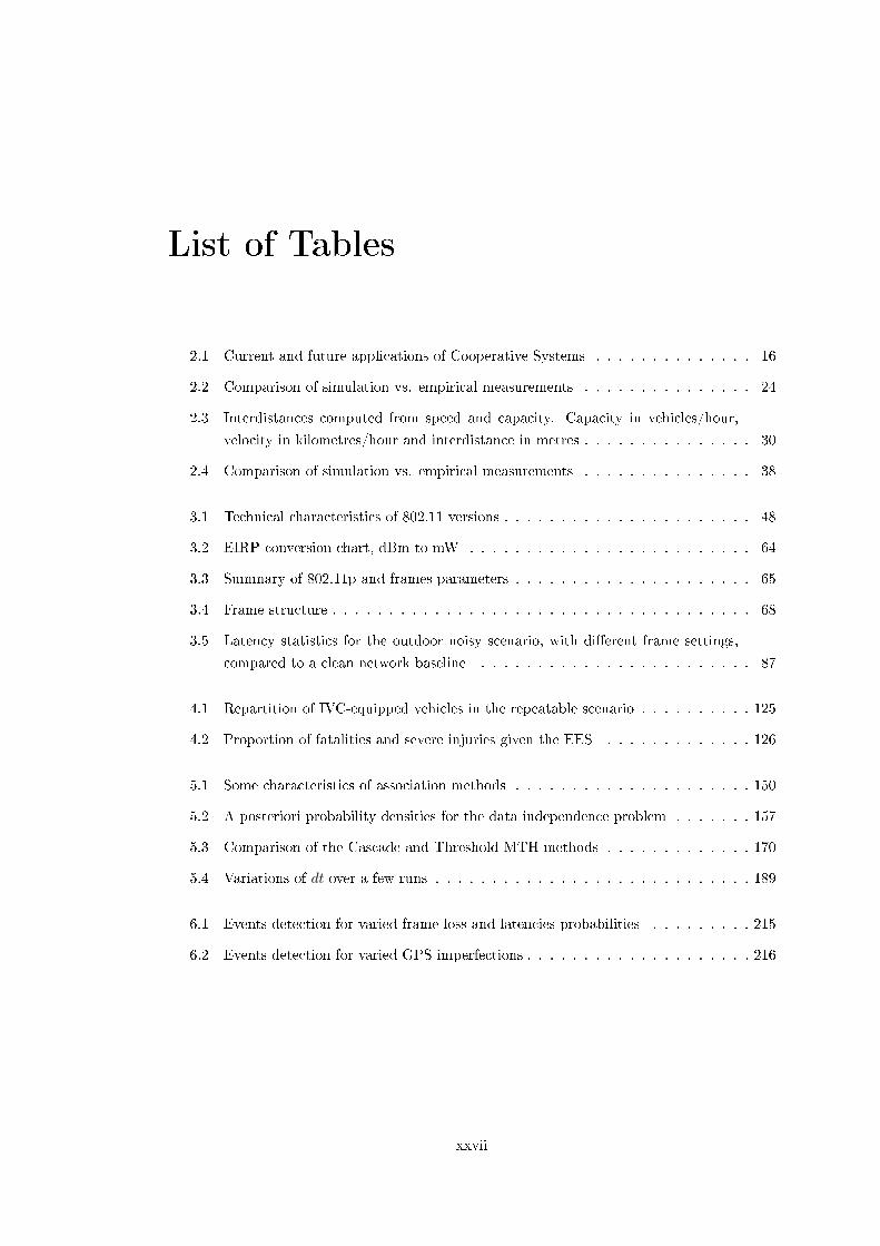
List of Tables

2.1 Current and future applications of Cooperative Systems . . . . . . . . . . . . . . 16

2.2 Comparison of simulation vs. empirical measurements . . . . . . . . . . . . . . . 24

2.3 Interdistances computed from speed and capacity. Capacity in vehicles/hour,

velocity in kilometres/hour and interdistance in metres . . . . . . . . . . . . . . . 30

2.4 Comparison of simulation vs. empirical measurements . . . . . . . . . . . . . . . 38

3.1 Technical characteristics of 802.11 versions . . . . . . . . . . . . . . . . . . . . . . 48

3.2 EIRP conversion chart, dBm to mW . . . . . . . . . . . . . . . . . . . . . . . . . 64

3.3 Summary of 802.11p and frames parameters . . . . . . . . . . . . . . . . . . . . . 65

3.4 Frame structure . . . . . . . . . . . . . . . . . . . . . . . . . . . . . . . . . . . . . 68

3.5 Latency statistics for the outdoor noisy scenario, with dierent frame settings,

compared to a clean network baseline . . . . . . . . . . . . . . . . . . . . . . . . 87

4.1 Repartition of IVC-equipped vehicles in the repeatable scenario . . . . . . . . . . 125

4.2 Proportion of fatalities and severe injuries given the EES . . . . . . . . . . . . . 126

5.1 Some characteristics of association methods . . . . . . . . . . . . . . . . . . . . . 150

5.2 A posteriori probability densities for the data independence problem . . . . . . . 157

5.3 Comparison of the Cascade and Threshold MTH methods . . . . . . . . . . . . . 170

5.4 Variations of dt over a few runs . . . . . . . . . . . . . . . . . . . . . . . . . . . . 189

6.1 Events detection for varied frame loss and latencies probabilities . . . . . . . . . 215

6.2 Events detection for varied GPS imperfections . . . . . . . . . . . . . . . . . . . . 216

xxvii

xxviii LIST OF TABLES

Nomenclature

BSS Basic Service Set; the basic building block of an 802.11 wireless LAN, expressed by the

name shared by all computers connected to this LAN

CALM Communication Access for Land Mobile; an integrated architecture supporting commu-

nication media and application diversity, and allowing many dierent communication

scenarios

CAN Controller Area Network bus; the message-based protocol designed for vehicle-embedded

microcontrollers and devices to communicate with each other without a host computer,

its deployment started in the later 1980s

CS Cooperative Systems

dBi dB(isotropic); the forward gain of an antenna compared with an hypothetical isotropic

antenna

dBm The power ratio in decibels of the measured power referenced to one milliwatt; it is an

absolute unit, by comparison, the decibel (dB) is a dimensionless unit

DFS Dynamic Frequency Selection; a mechanism allowing an IEEE 802.11 device to detect

and avoid frequencies used by some radar systems in order to limit interferences between

those systems

EDA Extended Driver Awareness framework; a Java-based development framework created

as part of the CVIS project

EEBL Emergency Electronic Brake Light

EIRP Eective Isotropically Radiated Power; given the radiated power observed in the maxi-

mum gain area of an antenna, the EIRP is the amount of power that would be radiated

by a theoretical isotropic antenna corresponding to produce the same output; the total

radiated power of the actual antenna will be smaller than the EIRP

ETSI European Telecommunications Standards Institute

FCC Federal Communications Commission, United States

GCDC Grand Cooperative Driving Challenge; a Dutch-lead European technological competi-

tion aiming at improving technologies related to cooperative driving, the rst challenge

was held in 2011

HMI Human Machine Interfacexxix

xxx

IFSTTAR Institut français des sciences et technologies des transports, de l'aménagement et

des réseaux (French institute of science and technology for transport, development and

networks)

IPv4 Internet Protocol version 4; fourth revision of the Internet Protocol, the connectionless

protocol for use on packet-switched Link Layer networks such as the Internet; IPv4 uses

a 4 bytes (32 bits) addressing system, IPv4 address exhaustion occurred on February 3,

2011

IPv6 Internet Protocol version 6; fth revision of the Internet Protocol, the connectionless

protocol for use on packet-switched Link Layer networks such as the Internet; IPv6 uses

a 16 bytes (128 bits) addressing system, IPv6 addresses are unlikely to ever run out

ITU International Telecommunication Union

IVC Inter-Vehicular Communication(s)

IVCD Inter-Vehicular Communication Device

LAN Local Area Network; a network of computers covering a limited geographic area or

nodes, from houses to an oce building; also a common term for a type of multiplayers

computer gaming

LIVIC Laboratoire sur les Interactions Véhicules-Infrastructure-Conducteurs (Vehicles-Infrastructure-

Drivers Interactions Laboratory), part of IFSTTAR

LoS Line of Sight

MAC Medium Access Control; a sublayer of the OSI model data link layer (layer 2), it provides

addressing and channel access control mechanisms allowing for several nodes to share a

common medium (wireless for example)

NTP Network Time Protocol; a classical time-synchronisation method for computers net-

works; it uses a pyramidal architecture (with strata, layers) of increasingly precise clocks

exchanging timing information through the network

OSI Open System Interconnection; standardised abstract layering model that groups similar

functions within a telecommunication architecture together; layers serves the one above

themselves and are served by the ones below

PHY Physical layer; the lowest layer of the OSI model (layer 1), where digital data are

converted to a physical signal that is transmitted over a hardware transmission medium

(wired or wireless)

QoS Quality of Service

RSU Roadside Unit; any ITS infrastructure (hardware) not embedded on a vehicle or located

in a major server room, contrasts with OBU (On-Board Unit)

RTK Real-time Kinematics; method to provide centimetre-level accuracy to satellite naviga-

tion systems, where a single reference ground station provides the real-time corrections

SSI Signal Strength Indicator

xxxi

UDP User Datagram Protocol; a communication protocol (included in IP) that allows the

exchange of messages (datagrams) without requiring prior communications to set up

special transmission channels or data paths, but providing no delivery guarantee

VANET Vehicular Ad-hoc Networks; more specic descriptor than MANET, Mobile Ad-hoc

Networks which can be applied to non-vehicular networks

WAVE Wireless Access in Vehicular Environments; the combination of the IEEE 802.11p and

IEEE 1609 standards covering the whole OSI layers

xxxii

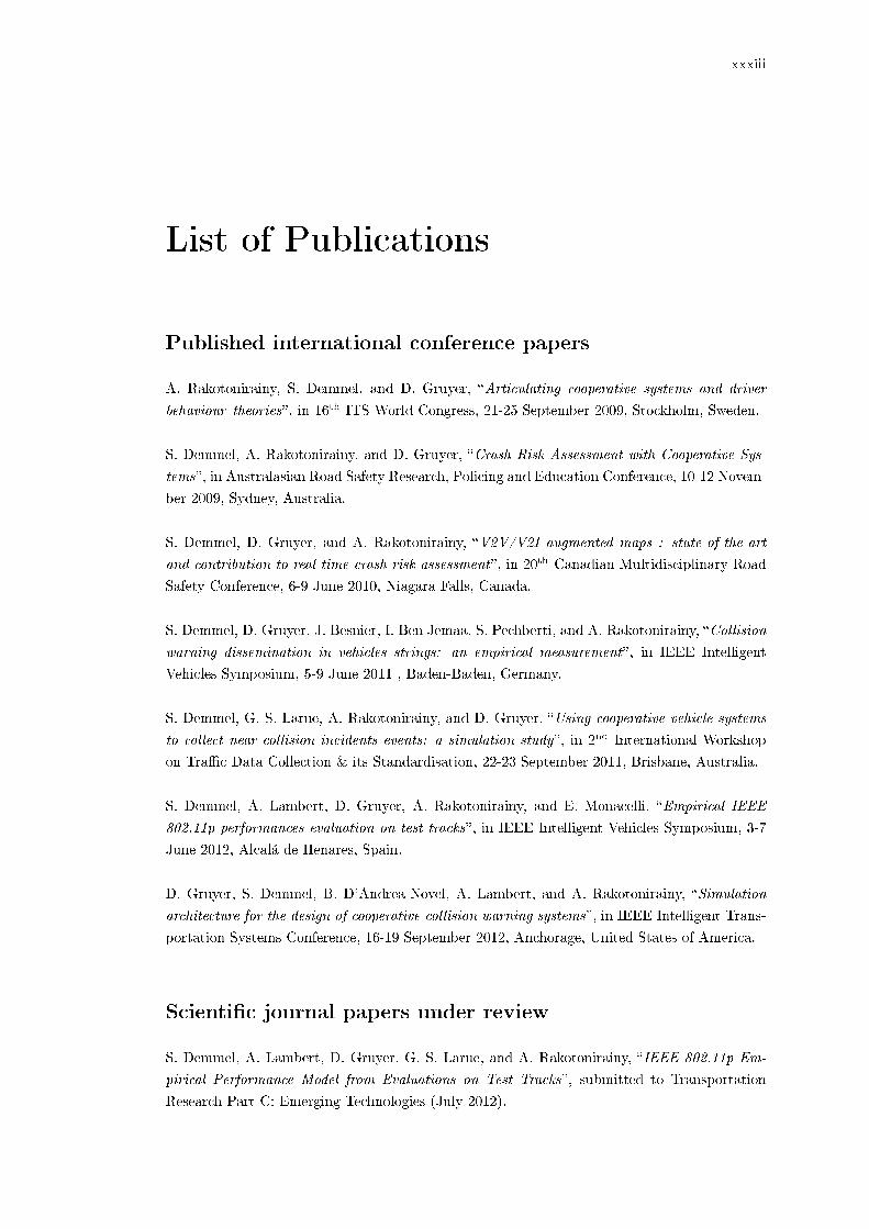
xxxiii

List of Publications

Published international conference papers

A. Rakotonirainy, S. Demmel, and D. Gruyer, Articulating cooperative systems and driver

behaviour theories, in 16th ITS World Congress, 21-25 September 2009, Stockholm, Sweden.

S. Demmel, A. Rakotonirainy, and D. Gruyer, Crash Risk Assessment with Cooperative Sys-

tems, in Australasian Road Safety Research, Policing and Education Conference, 10-12 Novem-

ber 2009, Sydney, Australia.

S. Demmel, D. Gruyer, and A. Rakotonirainy, V2V/V2I augmented maps : state-of-the-art

and contribution to real-time crash risk assessment, in 20th Canadian Multidisciplinary Road

Safety Conference, 6-9 June 2010, Niagara Falls, Canada.

S. Demmel, D. Gruyer, J. Besnier, I. Ben Jemaa, S. Pechberti, and A. Rakotonirainy, Collision

warning dissemination in vehicles strings: an empirical measurement, in IEEE Intelligent

Vehicles Symposium, 5-9 June 2011 , Baden-Baden, Germany.

S. Demmel, G. S. Larue, A. Rakotonirainy, and D. Gruyer, Using cooperative vehicle systems

to collect near collision incidents events: a simulation study, in 2nd International Workshop

on Trac Data Collection & its Standardisation, 22-23 September 2011, Brisbane, Australia.

S. Demmel, A. Lambert, D. Gruyer, A. Rakotonirainy, and E. Monacelli, Empirical IEEE

802.11p performances evaluation on test tracks, in IEEE Intelligent Vehicles Symposium, 3-7

June 2012, Alcalá de Henares, Spain.

D. Gruyer, S. Demmel, B. D'Andrea-Novel, A. Lambert, and A. Rakotonirainy, Simulation

architecture for the design of cooperative collision warning systems, in IEEE Intelligent Trans-

portation Systems Conference, 16-19 September 2012, Anchorage, United States of America.

Scientic journal papers under review

S. Demmel, A. Lambert, D. Gruyer, G. S. Larue, and A. Rakotonirainy, IEEE 802.11p Em-

pirical Performance Model from Evaluations on Test Tracks, submitted to Transportation

Research Part C: Emerging Technologies (July 2012).

xxxiv

xxxv

Statement of Original Authorship

The work contained in this thesis has not been previously submitted to meet requirements for

an award at this or any other higher education institution. To the best of my knowledge and

belief, the thesis contains no material previously published or written by another person except

where due reference is made.

Sébastien Demmel

Signature:

Date: 23/01/2013

QUT Verified Signature

xxxvi

xxxvii

Acknowledgements

I would like to thank my principal supervisors, Professor Andry Rakotonirainy and Associate

Professor Eric Monacelli, for having looked after me during these three years.

I would like to express my most sincere thanks to Dr Dominique Gruyer, my associate supervisor

and technical counsel from IFSTTAR-LIVIC. Without his timely intervention back in 2007, I

would never have considered moving to Australia, and probably neither doing a doctorate. He

has always been very helpful and supported my work, rstly as an intern, then as a doctorate

student.

I would also like to express my gratitude or appreciation to the people that have collaborated

with me during this research project, in France and Australia, and made possible the redaction

of this thesis; including Dr Grégoire Larue, Dr Alain Lambert, Joëlle Besnier, Inès Ben Jemaa,

Thouraya Toukabri, Jorge Godoy, and many others.

Eventually, I thank the AutoCRC for having supported this research through one of its post-

graduate scholarship.

xxxviii

xxxix

Personal dedication

To my parents, who have supported me over these 24 years as a student, from kindergarten to

PhD.

To my brother, who I am hopeful has nally found a career he enjoys.

To my grand-mother Irène, who passed away in August 2011 before she could see me nish my

doctorate.

To my friends, most of them from my teenage years in Hungary, Ala (also soon to be a doctor),

Laci, Bernas, Anne-Lise, Rami, Constance, Coco, FX, Irène, Angi, et cetera, et cetera; if I did

not write down your name, I did not forget you.

And eventually, a shout out to the crew of the Carco's, they will recognise themselves...

xl

Chapter 1

General Introduction

Foreword

This thesis positions itself within the context of a tri-lateral international cooperation between

the Queensland University of Technology (QUT) in Australia, the Université de Versailles Saint-

Quentin-en-Yveline (UVSQ) and the Institut français des sciences et technologies des transports,

de l'aménagement et des réseaux (IFSTTAR) in France. The research study has been made

possible thanks to the continued cooperation and shared research interests for half a decade

between the Centre for Accident Research and Road Safety at QUT and the Laboratoire sur

les Interactions Véhicules-Infrastructure-Conducteurs (IFSTTAR). As a result, this thesis will

combine both Australian and French perspectives on road safety research. Funding for this

study was provided by the Australian Cooperative Research Centre for Advanced Automotive

Technology (AutoCRC).

1.1 Rationale and Research Objectives

1.1.1 1970 to 2000: ghting road fatalities

Technological advances in the nineteenth and early twentieth centuries gave us a quick and easy

means to travel over vast distances that once seemed impossible i.e. the automobile. Human

civilisation and more modestly, people's daily lives, were fundamentally changed by this new

technological advent.

Unfortunately, automobiles also brought about a new form of mortality. If the rst death as a

result of a road crash goes back to the late nineteenth century, it is the democratisation of motor

vehicles that started in the second half of the twentieth century that led to an explosion in the

number of casualties on the road. The peak was reached in the 1970s, where the number of

fatalities literally sky-rocketed. For example, in 1970, no less than 16,000 people died in France

[1]; in the same year fatalities in Australia amounted to 3,798 [2] Projected over their respective

populations at the time (50.772 and 12.507 million respectively), fatalities reached 0.315 deaths

per thousand inhabitants in France, and 0.304 deaths per thousand inhabitants in Australia.

Overall, injuries, from the most to the least severe, have followed similar trends as fatalities.

To simplify matters, we will focus on fatality gures, knowing that measures implemented to

2 CHAPTER 1. GENERAL INTRODUCTION

reduce fatalities also have a similar eect on injuries. To illustrate this, the ratio of fatalities per

100 injuries remained constant between 1990 and 2004 [3], clearly showing that when fatalities

go down, injuries do so too.

Faced with such a dire situation on roads in the 1970s, governments initiated signicant regu-

latory eorts with the introduction of speed limits, compulsory three points seatbelts, alcohol

regulations, points system, etc. These regulations, combined with technological innovations

such as the ABS (1978), airbags (1981-87) and generally better built vehicles (with shock-

absorbing materials, etc.), helped to break the tide and bring fatalities numbers down. After

twenty years, in the early 1990s, fatalities had fallen in France to 10,483 [1], or 0.184 per

thousand inhabitants; and in Australia to 2,331 [2], or 0.137 per thousand inhabitants.

In the following two decades, technological and regulatory eorts have helped reduce the num-

bers and severity of road crashes from 10,483 in 1991, to 7,643 in 2000 and 4,092 in 2008 [1].

The latest French gures for 2010 record 3,992 fatalities, or 0.063 per thousand inhabitants [3].

A similar reduction took place in Australia, with the 2010 gures standing at 1,352 fatalities,

or 0.06 per thousand inhabitants [2]. In Europe, notably France, many lives have been saved by

the widespread deployment of automated roadside speed limits enforcement radars [4, 5, 6, 7],

but new in-vehicle technologies have also played a role, for example ESP (Electronic Stabil-

ity Program, also known as Electronic Stability Control) [8, 9]. This trend was largely made

possible by the increased aordability of in-vehicle electronics after the 1980s, which lead to

considerable research eort on driving assistance systems.

These systems have two tasks comfort and safety. For comfort, the system is designed to make

driving easier and more comfortable for the driver; technologies such as cruise control, parking

assistance, automated wipers and lights fall into this category. It can be argued that automated

gearboxes also provide comfort driving assistance. On the other hand, many driving assistance

systems have been developed solely to improve safety. It started with the ESP (1995) and

continued with automated cruise control (ACC, 1997), enhanced night-vision (2000-02), lane

departure alert (2001) and automated pre-crash braking (2003).

By early 2010s, most of these aforementioned systems were available in high-end mainstream

vehicles, and not just luxury vehicles. More sophisticated systems, which are close to being

available commercially, involve semi-automated driving such as low-speed automated control

in trac jams [10], co-pilots that do not only take control of the vehicles in some settings but

also rank potential manoeuvres on their risk and legality [11], or an Emergency Stop Assistant

[12] that can safely park a vehicle if the driver becomes suddenly incapacitated. At times,

the distinction between safety and comfort driving assistance can become blurred. This is for

example the case with ACC. ACC uses a forward-facing radar to adapt the driver's speed input

to the driving context. The system provides both comfort (cruise control) and safety (respecting

safety distances and enhanced braking reaction) benets [13, 14]. Generally, comfort-orientated

systems may have safety benets, but these are often secondary to their initial comfort task.

1.1.2 The great leap forward: Cooperative Systems

Despite the excellent results described in the previous subsection, recent statistics show that

the decreasing trend in fatalities has stopped and stagnated [15]. In France, between 2008 and

2011, the number of fatalities only decreased by 305, while decreasing by 1,043 between 2005

and 2008. This suggests that technological research in safety-orientated driving assistance needs

1.1. RATIONALE AND RESEARCH OBJECTIVES 3

to go further in providing additional benets and to continue sustaining the fatalities-decreasing

trend.

The answer to this problem is in the form of Cooperative Systems (CS). In the broadest sense,

CS describe a family of Intelligent Transportation Systems (ITS) where several actors of the

road environment cooperate to perform a task. Road actors can be vehicles (and their drivers),

roadside intelligent infrastructure, pedestrians, etc. Cooperation between road actors provides

multiple information sources.

As a matter of fact, current non-cooperative driving assistance systems combine more and

more information from diverse sources to provide better services to drivers. Typically, this has

meant an increase in the number of in-vehicle sensors, with multiple cameras, laser telemeters,

radars, etc. Information is analysed using various mathematical methods and algorithms such as

Kalman ltering, fuzzy logic or the Dempster-Shafer Theory (also known as the Belief Theory).

With such enhanced perception and driving assistance systems, drivers ultimately become more

aware of their environment. However, because of inherent limitations in range and eld of view,

the systems' perception of the environment remains largely limited to a small interest zone

around the ego-vehicle1.

CS aim at compensating such limitations with the fusion of embedded information technology

and intervehicular communication technology. Such a combination would bring the advent

of decentralised information managing systems for driving assistance and road safety which

would not be limited to a single vehicle anymore. The formation of the Wi-Fi Alliance2 in

1999, to market the IEEE 802.11a and 802.11b standards, marked the point at which wireless

communication technology became aordable to the average household consumers and as a

result, the point at which CS became a realistic perspective.

CS have already gathered a lot of interest from the research community in the main automotive-

making regions of Europe, Japan and the USA. Many large projects, often multinational in the

case of Europe, have been dedicated to them in the safety area: COOPERS, SAFESPOT and

CVIS in the European Union [16]; DSSS in Japan [17]; and PATH, CICAS-V and IntelliDrive

in the USA [18, 19, 20]. Many potential applications to such technologies have been envisioned:

cooperative trac management, crash prevention, real-time road and trac state information,

variable speed limits, etc. For example, one of the most straightforward safety-related CS

applications is termed Emergency Electronic Break Light (EEBL) [21]. It uses radio links to

transmit a message alerting drivers that an emergency braking event is taking place ahead of

them, so that they can prepare to brake when the braking wave reaches them. Simulations

show that using EEBL is sucient to lead to substantial fatalities reduction [22, 23].

However, CS will typically be more complex than EEBL. Indeed, by networking road actors

one can go further than classical in-vehicle driving assistance systems thanks to the distribution

of information sources and data processing capabilities. From this distribution of information

sources, the concept of extended or augmented perception arises.

Augmented perception allows extending an actor's perceptive horizon beyond its natural

limits, not only with information from multiple in-vehicle sensors but also information obtained

from remote sensors. The perceptive horizon is dened as the limit between the environment

part that can be perceived by in-vehicle sensors (the scene) and the other parts that cannot be

1The ego-vehicle is a vehicle where the focus of a system is made: for example with a collision preventionapplication, the vehicle which gathers information about its surroundings to analyse other objects' trajectoriesand their collision risk.

2http://www.wi-.org/

4 CHAPTER 1. GENERAL INTRODUCTION

Figure 1.1: Layered augmented map concept

perceived. This covers the maximum range of sensors and occultation (shadowing) by objects in

the scene that block direct line of sight. By bringing in data from other sensors that have another

point of view on the environment, augmented perception provides applications with information

they would not have access to if limited to a single point of view (the native perception

horizon). Furthermore, an actor can also share information that external sensors have no way

of measuring; for example, physiological data about the driver. Eventually, the underlying data

fusion mechanisms increases the precision, reliability and robustness of information extracted

from the environment, whether from inside or outside the horizons of native perception

The end result of an augmented perception and data fusion chain is known as an augmented

map. It is a repository where any relevant information about objects in the environment, and

the environment itself, can be stored in a layered architecture (see Fig. 1.1). One layer can,

for example, include a map of moving objects detected in the environment, each described by

a set of attributes (their state vector). Afterwards, the augmented map is made available to

driving assistance systems and drivers to enhance their perception of the environment. It can

be used in many dierent ways, for example, to enhance a driver's perception of what is going

on a few vehicles ahead in dense trac. It can also feed a collision risk computation application

that will benet from a better representation of the road, and even allow cooperation between

actors to actively avoid an impending crash.

Augmented perception is especially relevant to the accidentology. Indeed, statistics show that

crashes are mostly driven by human error [24], compared to other factors such as environmental

conditions and mechanical defects. Within human errors, the dominant error source is percept-

ive errors, which represent about 50% of the total [25]. The next two sources are interpretation

and evaluation, which together with perception, accounts for more than 75% of human error

related crashes. This shows that allowing drivers to perceive and understand their environment

better, or supplement them when they are clearly at fault, is a solution to a good assessment

of road risk, and as a consequence, can further decrease fatalities.

It is important to note that care should be taken in the way drivers are presented with the

additional information provided by augmented perception. Indeed, drivers are at risk to be

overwhelmed by information from outside their natural perceptive horizon. Similarly, they

could be distracted by this information and overlook other critical information. Thus, there

1.1. RATIONALE AND RESEARCH OBJECTIVES 5

is a research opportunity here to nd ecient and appropriate solutions to convey augmented

information to drivers. However, this falls outside the scope of the present research.

1.1.3 Research Objectives & Scope

The aim of this thesis is to identify road risks by using distributed information extracted from

an augmented map thus, demonstrating that cooperative systems-based safety applications

have better performance than non-cooperative ones. However, before computing risks, it is

necessary to evaluate the limitations of augmented perception, in general, and augmented maps

in particular. Indeed, while many promising results have already been obtained, the feasibility of

building an augmented map from exchanged local perception information and, then, being able

to use this information benecially for road users, has not been thoroughly assessed. Notably,

many questions remain unanswered as to the telecommunications performance and their ability

to deliver appropriate quality of service to support life-saving critical systems. The aim of this

research can be summarised with the following research questions:

1. How can crash risk be assessed in real-time with an augmented map built from local

sensors' data gathered from multiple vehicles?

2. Can an augmented map-based risk assessment system be more ecient than a similar

non-cooperative system?

3. What are augmented perception's limitations, given current technology in embedded com-

puting and telecommunications?

One needs to demonstrate whether cooperative systems can indeed be more ecient than their

non-cooperative equivalents to detect and evaluate risky driving situations. Thus, it is import-

ant to show what limitations current technology introduces for the CS. It can be argued that

inecient intervehicular communications may render the benets from introducing information

sharing null. This is especially true as the road environment is a complex, highly variable

setting where many sources of imperfections and errors exist, and not only for wireless commu-

nications. In order to take into account these sources of imperfections, this thesis has a strong

empirical avouring, basing itself on concrete measurements.

Before proceeding further along this chapter, it is important to state what will be considered as

out of scope of this research thus, will not be covered in this thesis. Essentially, all the human

factors (HF) aspects of Cooperative Systems will be excluded from this research. This concerns

the Human-Machine Interface (HMI); even though more research is necessary to determine how

to eciently convey the drivers additional information that is obtained with CS, we will not be

interested in this aspect rather, focusing on the technical challenges that come with CS. Other

HF aspects that are outside the scope of this research concerns dierences in driver behaviour

on the road and their interaction with safety systems, or what will be the eect of augmenting

the driver's awareness of their environment, on their behaviour. Although these aspects are

out of the scope of this thesis, our work will still have implication for them; further details

regarding these implications will be discussed in the general conclusion in Chapter 7.

1.1.4 Approach

Firstly, we need to answer a few questions regarding the research methodology that we will use

to study the performance of augmented maps. Indeed, our requirements can be addressed using

6 CHAPTER 1. GENERAL INTRODUCTION

two dierent manners of equal a-priori outlooks: (1) on one hand, advanced simulations and

(2) on the other hand, actual full on-road implementation in a research setting. We note there

were unknown quantities (within the specic context of CS) aecting the empirical methodo-

logy in terms of its advantages and disadvantages versus the simulation methodology. Given

these unknown quantities, and the availability of appropriate resources (hardware, drivers, etc.)

at the LIVIC laboratory, our rst step in the research approach is to evaluate the empirical

methodology to ll the missing gaps and lead to a more informed choice. To do so, we imple-

mented an EEBL scenario on the Satory test tracks located in the city of Versailles, France.

The results from this implementation showed that it was unwarranted to continue with the

EEBL implementation, in particular, and with a fully empirical research methodology, because

it was dicult to obtain meaningful results on the safety benets of the system being studied.

Thus, we selected a research methodology focused on advanced simulations, but still taking

into account improvements brought by empirical research on the performance of wireless com-

munication technologies.

As we mentioned, CS aim at deploying an integrated wireless network between road actors

- vehicles and additionally, roadside infrastructure. Although wireless communications need

not be radiofrequency only (infrared communication have been suggested), they do dominate

the eld. In 2010, the IEEE adopted an amendment to the 802.11 standard, 802.11p [26],

which is specically dedicated to enhancing 802.11 technology for the road environment. This

amendment was released in the latest version of the standard (IEEE 802.11-2012) alongside

others [27]. Performance evaluation of 802.11p is an ongoing area of research, into which it is

necessary to delve when considering the eciency of Cooperative Systems.

Our approach consists of, rstly, evaluating the empirical performance of IEEE 802.11p tele-

communications in close-to-real-road settings on the Satory test tracks. Our evaluation process

allowed us to dene a set of boundaries on the performance that one can expect from this tech-

nology. Importantly, it showed that many assumptions made on the usefulness of CS for safety

tasks may have been over-optimistic, especially in terms of the connection ranges that 802.11p

systems can achieve. This is further aggravated by the fact that we obtained these results in a

relatively open and controlled freeway-like environment, and not on actual roads, where sources

of imperfections are omnipresent. The considered performance metrics were latency, frame loss

and range.

We used results from the evaluation process to build a representative, yet straightforward,

empirical model of 802.11p performance metrics; environmental factors such as the weather

as well as performance variations introduced by hardware inhomogeneities (for example, non-

omnidirectionality in antennas) were taken into account. The proposed model is particularly

well adapted to higher-level simulations of CS applications with up to a dozen road actors. It

is complementary to more detailed networking models such as the one used in the well-known

ns-x family of simulators.

Consecutively, we developed a CS simulation architecture in the SiVIC sensor simulator [28].

This architecture is very versatile, and can be used to simulate simple CS applications, or to

build an augmented map. At rst, we developed an EEBL application inside this architecture,

which we use to validate it in a reproducible reference scenario. We selected a freeway vehicles

string as our reference driving scenario, leading to rear-end crash-prone situations. Rear-end

crashes represent between one fth and one third of all road crashes (depending on regions

and countries) [29, 30]. Furthermore, more than half (56.4%) of the drivers do not follow safe

interdistances recommendations (at least 2 seconds) in dense trac [3]. For these reasons,

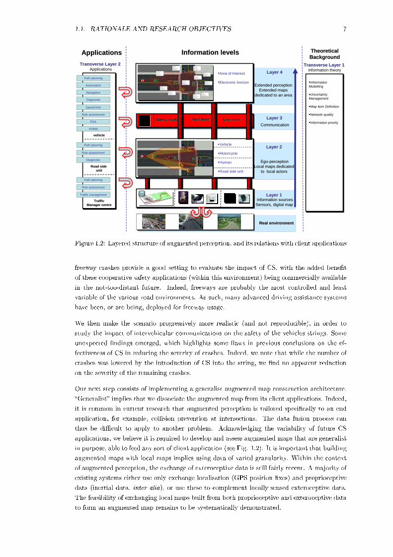
1.1. RATIONALE AND RESEARCH OBJECTIVES 7

Information sourcesInformation sourcesSensors, digital mapSensors, digital map

EgoEgo--perceptionperceptionLocal maps dedicatedLocal maps dedicated

to local actorsto local actors

CommunicationCommunication

Extended perceptionExtended perceptionExtended mapsExtended maps

dedicated to an areadedicated to an area

Transverse Layer 1Transverse Layer 1information theory

Real environmentReal environment

Transverse Layer 2Transverse Layer 2Applications

Area of InterestElectronic horizon

Safety levelSafety level Alert levelAlert level User levelUser level

VehicleMotorcycleHumanRoad side unit

InformationModellingUncertainty ManagementMap item DefinitionNetwork qualityInformation priority

vehiclevehicle

Road side Road side unitunit

TrafficTrafficManager centreManager centre

Layer 4Layer 4

Layer 3Layer 3

Layer 2Layer 2

Layer 1Layer 1

Information levelsInformation levels TheoreticalTheoreticalBackgroundBackground

ApplicationsApplications

Path planning

Automation

Navigation

Diagnostic

Speed limit

Risk assessment

EDA

POMA

Path planning

Risk assessment

Diagnostic

Path planning

Risk assessment

Traffic management

Figure 1.2: Layered structure of augmented perception, and its relations with client applications

freeway crashes provide a good setting to evaluate the impact of CS, with the added benet

of these cooperative safety applications (within this environment) being commercially available

in the not-too-distant future. Indeed, freeways are probably the most controlled and least

variable of the various road environments. As such, many advanced driving assistance systems

have been, or are being, deployed for freeway usage.

We then make the scenario progressively more realistic (and not reproducible), in order to

study the impact of intervehicular communications on the safety of the vehicles strings. Some

unexpected ndings emerged, which highlights some aws in previous conclusions on the ef-

fectiveness of CS in reducing the severity of crashes. Indeed, we note that while the number of

crashes was lowered by the introduction of CS into the string, we nd no apparent reduction

on the severity of the remaining crashes.

Our next step consists of implementing a generalist augmented map construction architecture.

Generalist implies that we dissociate the augmented map from its client applications. Indeed,

it is common in current research that augmented perception is tailored specically to an end

application, for example, collision prevention at intersections. The data fusion process can

thus be dicult to apply to another problem. Acknowledging the variability of future CS

applications, we believe it is required to develop and assess augmented maps that are generalist

in purpose, able to feed any sort of client application (see Fig. 1.2). It is important that building

augmented maps with local maps implies using data of varied granularity. Within the context

of augmented perception, the exchange of exteroceptive data is still fairly recent. A majority of

existing systems either use only exchange localisation (GPS position xes) and proprioceptive

data (inertial data, inter alia), or use these to complement locally-sensed exteroceptive data.

The feasibility of exchanging local maps built from both proprioceptive and exteroceptive data

to form an augmented map remains to be systematically demonstrated.

8 CHAPTER 1. GENERAL INTRODUCTION

The augmented map building architecture is implemented in SiVIC, supported by our earlier

model of 802.11p performance. Using SiVIC allows us to create a very realistic simulation that

integrates a wide range of imperfections. Data fusion is performed using Kalman ltering and

the Dempster-Shafer Theory, as a follow-up to previous works concerning the adaptation of these

mathematical principles to augmented perception [31]. We use this architecture to study the

performance of CS versus non-cooperative systems to assess the risk of a driving situation (our

reference scenario). Results show that the CS-based approach consistently provides advanced

warning to drivers during an emergency braking event compared to the non-CS based approach,

despite the limitations introduced by imperfect telecommunications.

Eventually, we developed a dedicated simulation to demonstrate the ability of CS to be used

to detect near-miss events, as a further step towards assessing risks using CS. Near-misses or

near-collisions, are a common crash surrogate measurement. An evaluation of augmented map-

based risk-assessment is performed within the same reference scenario, to compare cooperative

and non-cooperative approaches, highlighting the benets of the cooperative approach.

Overall, this research approach allows us to conclude on the merits of CS that is solidly grounded

in reality, and not only on potential merits that is assumed from simulations.

The research approach described in this section is also summarised in graphical form in Fig. 1.3.

Research problems, the dierent research tasks and their results are paired with the relevant

chapters (for more details, see 1.2). The relationship between each aspect of the thesis is shown

with arrows linking them; the arrows are directed to show the hierarchy that exists between each

section and which task inuences the other (for example, how the implementation performed

in a specic task was later used in another implementation).

As an example, if we consider the blue box building an augmented map? , it covers a sub-

question of our rst research question, and leads to the third research question (the blue box

CS/IVC performance? ); this second question is the central theme for Chapter 3, leading

to the performance evaluation of 802.11p on the tracks and the construction of an empirical

performance model. The building an augmented map? box is answered in Chapter 5 together

with the design of the augmented map-building architecture.

1.1.5 Contributions

This thesis' contributions span several research disciplines, from vehicular wireless networks,

simulation of driving assistance systems and data fusion . They are classied and explained

further in the remainder of this section.

V2V/I evaluation

A comprehensive evaluation of V2V/I telecommunication technology (802.11p) was performed

on the track in a close-to-real-road setting, demonstrating that while V2V/I is indeed suitable for

safety cooperative applications, its performance with average hardware have been overestimated

by previous studies. Indeed, performance showed a large variability even within the relatively

controlled environment of Satory's test tracks.

Relevant sections: chapter 3, sections 3.3 to 3.6

1.1. RATIONALE AND RESEARCH OBJECTIVES 9

Figure

1.3:Graphicalrepresentationofthethesis'approach

andstructure

10 CHAPTER 1. GENERAL INTRODUCTION

V2V/I implementation

As part of the aforementioned V2V/I evaluation, an implementation of 802.11p-enabled devices

and of an EEBL application was completed. This open source implementation is adaptable and

fully controllable, and can be used to support further research. As a matter of fact, several

technological demonstrations utilised this system in 2011 and early 2012.

Relevant section: chapter 3, section 3.5

V2V/I modelling

This thesis provides a new empirical 802.11p performance model which is aimed at being used

by higher-level simulations of CS applications, contrary to most existing models that are focused

on lower-level network simulations.

Relevant section: chapter 3, section 3.7

Cooperative Systems simulation architectures

A complete CS simulation architecture was designed and implemented as part of this thesis,

within the SiVIC-RTMaps simulation framework. The programming language used is C++.

This architecture is versatile and can be easily modied to accommodate other research on CS.

It provides major improvements in terms of realism, compared to previous architectures.

Relevant sections: chapter 4, sections 4.1 to 4.4

Generalist augmented map building architecture

A generalist augmented map building architecture was designed and implemented as part of

this thesis, within the SiVIC-RTMaps simulation framework. It uses data from simulated

scenarios generated with the aforementioned CS simulation architecture, or data recorded from

real vehicles. An emphasis is placed upon independence from client applications, and thus

increasing its versatility in the architecture. The programming language used is C++. The

architecture also builds upon previous research to adapt the Dempster-Shafer theory to data

fusion problems within the specic context of augmented perception.

Relevant sections: chapter 5, sections 5.3 and 5.4

Benets of CS for road safety

This thesis nds new insight on the safety benets of CS in general, and augmented maps

in particular. We demonstrate that they can be more useful than non-cooperative systems

in assessing road risks in certain conditions, typically in warning drivers in advance of an

impending crash in vehicles strings. We also demonstrate that they can be used to record

useful data about near-collision events in a naturalistic driving setting. However, we also

show that potential benets might have been over-estimated by previous research. Reduced

communications performance at high relative speed means that in such conditions CS do not

perform any better than non-cooperative systems. Furthermore, we nd that a typical EEBL

application had no benets according to a crash severity criterion based on the EES.

1.2. THESIS OUTLINE 11

Relevant sections: chapter 3, section 3.6; chapter 4, sections 4.4 and 4.5; chapter 5, section

5.5; chapter 6, section 6.4

1.2 Thesis Outline

Chapter 2: Studying the safety benets of Cooperative Systems After laying out

the research methodology problem, chapter 2 presents a literature review of CS applications,

especially regarding safety-related ones, and introduces the reference on-road scenario that we

will use for the remainder of this thesis. Then, it discusses the merits of empirical-focused

research versus simulations-focused research and explains why we choose, at rst, to implement

an on-road study of a CS application (EEBL). Then it discusses the design, implementation

and mixed ndings of this real-world implementation of EEBL which involves four vehicles.

Eventually, it concludes on the rationale for selecting the simulations, which we will improve

using empirical data, as our principal research methodology.

Chapter 3: Evaluation of telecommunications for augmented perception Chapter 3

begins with a literature review regarding V2V/I telecommunication technologies in general, and

IEEE 802.11p in particular to present in further detail the context of the present research and

how it is essential to CS. The experimental design (setups and scenarios) for the performance

evaluation is then explained, before the analysis of the chosen performance metrics. From this

analysis, chapter 3 moves forward to the development of an empirical 802.11p performance

model, of which several dierent versions are presented. Eventually, we discuss ndings such as

the telecommunications' limitations and, especially, the unwarranted optimistic expectations of

previous research.

Chapter 4: Simulation architecture for Cooperative Systems applications Chapter

4 introduces our CS simulation architecture in the SiVIC simulator and the RTMaps multi-

sensors prototyping platform. Validation of the simulation architecture compared to previous

research is described. Eventually, new results are discussed, notably regarding the reduced e-

ciency, regarding the crash severity (EES) criterion, of a typical EEBL application implemented

with our CS simulation architecture.

Chapter 5: Building an augmented map Chapter 5 begins with a literature review on

data fusion for local and augmented perception in order to provide some context. Then, it details

the map building architecture we implemented in SiVIC, including its theoretical foundations,

most notably the adaptation of the Dempster-Shafer Theory to augmented perception problems.

Eventually, it oers a performance analysis of a simple risk-assessment approach using our map-

building architecture versus non-cooperative local maps, taking into account the limitations

determined in Chapter 3.

Chapter 6: Towards risk assessment: an application Chapter 6 presents, at rst,

a literature review of studies on near-misses and their relationship to classic risk assessment,

as well as how augmented perception can be used to solve research problems surrounding

the detection and classication of near-miss events. Then, it discusses the design and results

12 CHAPTER 1. GENERAL INTRODUCTION

obtained from a dedicated simulation of near-miss events detection using CS, demonstrating its

advantages compared to non-cooperative approaches.

Chapter 7: General Conclusion Chapter 7 concludes the thesis with a summary of the

work presented in previous chapters and continues on to discuss issues and insights that have

been identied in the course of this research, along with paths for future research.

Appendix A: Experimental documentation Appendix A provides for reference the uned-

ited (in French) and translated experimental documents that were written over the course of this

research for later reference as well as to allow other researchers to reproduce the experiments.

Experimental implementation of the EEBL scenario is covered, as well as the installation of

802.11p-enabled IVC devices.

Chapter 2

Studying the safety benets of

Cooperative Systems

2.1 Introduction

One of the principal aims of this thesis is to evaluate the limitations of augmented perception,

particularly augmented maps within the context of their potential contribution to the safety of

road users. In the initial chapter, we argued that while many promising results have already

been obtained, the feasibility of building an augmented map from exchanged local perception

information had not been thoroughly assessed, and that it was necessary to show whether

applications using augmented perception are more ecient than non-cooperative applications.

In order to do so, an appropriate research methodology is selected which will provide results on

benets of augmented perception that are realistic enough to withstand scrutiny. The research

methodology must provide conditions that are similar to the future conditions into which the

studied applications are likely to be deployed, as well as the conditions of current applications

with which they will be compared. These requirements are not straightforward, and can be

answered in two dierent manners of equal a-priori outlooks using advanced simulations that

may be supported by empirical data or full on-road implementations in a research setting. This

should not be seen as being limited to augmented perception only but can be applied to any

type of applications oered by Cooperative Systems (CS).

The aim of this chapter is to select the most appropriate research methodology. Neither of the

competing methodologies are superior to the other, a-priori, but are actually complementary

as one can be used to support the other for some specic tasks. We identied some gaps in

the merits of the fully empirical methodology, notably, its disadvantages were not clearly laid

out. Concerns were raised in relation to the limitations that might arise when implementing a

system on real vehicles and hinder the process of our research on that system's safety benets.

Given the availability of test hardware at the LIVIC laboratory, we chose to perform an initial

evaluation of these potential issues by implementing an Emergency Electronic Break Light

(EEBL) application on the Satory's test tracks. This implementation had two goals: (1) validate

the use of an empirical research methodology for future CS-related research (and identify its

weaknesses); and (2) empirically conrming previous research on the contribution of IVC to

the safety of vehicles' strings.

14 CHAPTER 2. STUDYING THE SAFETY BENEFITS OF COOPERATIVE SYSTEMS

Previous studies on EEBL, one of the most straight forward safety-related CS applications,

have shown promising safety benets even with a limited number of vehicles equipped with the

system. These studies were undertaken in dedicated simulations in which assumptions about

the performance of IVC, vehicles and drivers were done. We decided to test the validity of the

IVC safety benets in an imperfect semi-realistic1 environment, in terms of IVC and vehicle

performance, by implementing an EEBL application on Satory's test tracks.

The diculty in evaluating CS applications on track (or on the road) without important invest-

ments will be demonstrated in this chapter. The implementation was challenging in terms of

engineering experience but yielded interesting preliminary results that were used in preparation

for the IEEE 802.11p performance study which is covered in Chapter 3. The results provided

data on the performance of IEEE 802.11g telecommunication that can be used as a bench-

mark for future empirical investigations, as well as design for a common software and hardware

architecture for on-track measurements.

However, the outcome of the validation of IVC safety benets was not conclusive, with a num-

ber of logistical and experimental protocol limitations exposed during the experiment. This led

to the conclusion that advanced simulations should be used as the main method to address our

research problems. We also concluded that it was necessary to provide models based on empir-

ical data for these advanced simulations, to increase output quality and relevance, in relations

to the performance and benets of safety critical CS applications. Designing an advanced CS

simulation architecture and collecting the empirical data to support its modelisation of IVC

performance will be the focus in the two following chapters.

Chapter Outline

The rst section presents a concise review of Cooperative Systems (CS) focusing on the proposed

or existing safety applications. To provide further context, this section discusses the safety

benets of CS followed by the introduction of a vehicle strings scenario since it will be used

extensively as a reference for the on-road implementation as well as for future simulations.

In the second section, we will discuss the rationale and issues surrounding the methodology

settlement in more detail.

The third section presents the design and implementation of a simplied on-road EEBL

system, aiming at validating its safety benets in an imperfect environment.

Then, the fourth section discusses the results of a four-vehicle test on the Versailles-Satory's

tracks, showing the complexities surrounding such implementation, as well as the diculty of

obtaining meaningful results without actually extending into unsafe driving situations.

In conclusion, the fth section covers the rationale and motivations for focusing on simulations

to assess CS's safety benets, especially the most advanced ones.

1The Satory tracks can be presumed to be semi-realistic because they are not open to normal trac

2.2. LITERATURE REVIEW AND STATE-OF-THE-ART 15

2.2 Literature review and state-of-the-art

2.2.1 Cooperative Systems: a wide potential

As argued in Chapter 1, Cooperative Systems can be seen as the technological answer to the

current problem of stagnating fatality rates on roads in First World nations. In the broadest

sense, CS describe a family of Intelligent Transportation Systems (ITS) where several actors

involved in the road environment such as vehicles, roadside intelligent infrastructure or ped-

estrians, cooperate to perform a task. Eventually, research aims at creating an integrated

network between the aforementioned actors based on wireless communications. The underlying

technologies required to support a cooperative architecture and most notably 802.11p will be

addressed in Chapter 3. In this section, we will concentrate on the applications and benets,

especially the safety benets of CS.

Using wireless communications, of any form, to allow in-vehicle and roadside systems to cooper-

ate can lead to many potentially useful applications, of varying complexities. Many of them do

not have safety aspects and the applications that are on the consumers market are often exten-

sions of existing non-cooperative applications. In Table 2.1 (from [32, 33] and other sources),

we list applications which have been deployed, are currently in research and development stages

(at various levels of advancement) and potential applications which are still more remote, with

possible commercial availability well into the 2020s.

Electronic tolling (ETC) and cooperative driving (platooning) are the oldest forms of CS.

ETC has been widely deployed in the late 1990s and 2000s. Earliest examples are found in

Norway in 1986 and the USA in 1989. The rst truly unassisted ETC system was deployed

in Trondheim, Norway in 1991 [34]. The rst fully automated toll freeway, Ontario Highway

407 (Express Toll Route), opened in Canada on 7 June 1997. It provided an early example

of CS integration with other ITS systems, as the ETC system on Highway 407 combines RF

transponders with roadside cameras for automatic number plate recognition[35]. Platooning

and cooperative driving research began more than 20 years ago [36, 37, 38, 39]. Although,

the most advanced concepts related to platooning have not found their way in the market at

present, cooperative driving in the form of CS-enhanced autonomous cruise control system is

currently in active research. Signicant safety and comfort benets are expected from these

enhanced systems.

Another type of cooperative application that is likely to be desired by the general public is

infotainment, also known as In-Car Entertainment (ICE). With constant connectivity made

available with smartphones and other mobile devices, it is relatively logical to use the vehicle's

capability to support more advanced forms of online activities however, some sources have spec-

ulated that the ICE will not be as popular as expected because of the prevalence of smartphones

and the potential cost of ICE services. Currently, the existing ICE services (provided by Ca-

dillac and Chrysler) uses 3G mobile phone connections to reach the outside network but these

technologies have limitations (refer to Chapter 3). Seamless access to the Internet and espe-

cially social media and video sharing platforms might be achieved by dedicated infrastructure

provided within a CS context [40, 41].

However, neither ETC nor ICE should be perceived as the principle potential of cooperative

applications. The main potential of CS, which is gathering the most research interest, lies in

its ability to extend one road actor's perceptive horizon, which is achieved from the fusion of

information obtained from a multitude of remote and local sources.

16 CHAPTER 2. STUDYING THE SAFETY BENEFITS OF COOPERATIVE SYSTEMS

Table 2.1: Current and future applications of Cooperative Systems

Category Application

Electronic tollingElectronic toll collectionAdaptive toll collection

Adaptive insurance (pay-as-you-drive)

Trac managementAdaptive trac re-routingEmergency services (eCall)

Remote sensing of breakdowns and crashes

Fleet managementTrade vehicles (delivery services, freight)

Public transports vehiclesTaxis

TrackingEmergency vehicles

Funds, precious or dangerous goods

Regulations enforcement or information

Intelligent Speed AdaptationEmergency lane usageRight of way rules

Banning of specic manoeuvres/actions

Incident and threats warning

Collision preventionCrash and breakdown warningWeather and road conditions

Ghost driver warning

Infotainment servicesIn-vehicle high-speed Internet

House-vehicle networking link (domotics)

Other servicesRemote diagnosticRemote update

Geo-activated services (advertisement, ...)

Perceptive horizon is dened as the limit between the part of the environment that one can

access with its sensors and the part of the environment that is inaccessible. The term scene

is also used to describe the area bounded by the perceptive horizon. Maximum range and

occultations by objects both dene the boundaries of the perceptive horizon. For a driver,

the perceptive horizon is broadly the limit of their eld of view, in depth as much as angular

opening. Technically the range of the eyes could be described as innitewe can see light

emanating from sources located thousands of billions kilometres away, e.g. stars (1 light-year

is about 1013 kilometres, the closest star is located 4.22 light-years away)but in practice it is

limited by resolution. Vehicle-embedded sensors for mono-vehicle ADAS can extend this natural

perceptive horizon but this is not always the case, nor is it required by their specications. For

example, a radar has a range of about 200 metres so it does not really extend the driver's

perceptive horizon to objects further than this distance.

CS can thus be used to provide perception augmentation to road users such as drivers. Per-

ception augmentation covers both perception extension and perception enrichment. Perception

extension simply consists of obtaining data from areas that are outside the perceptive horizon,

as described in the previous paragraph. On the other hand, perception enrichment consists of

obtaining information about an object that a given set of external sensors cannot measure from

a distance. For example, no sensor can remotely measure the vigilance state of other drivers

thus, obtaining some information about this state is a form of perception enrichment. Similarly,

transmitting the state of pedals to other vehicles is a form of perception enrichment.

The subject of perception augmentation by CS, independently of the applications that it could

support, is well covered in the literature. To quote a few examples, Wender and Dietmayer

[42] combined an ego-vehicle embedded laserscanner with positioning data transmitted from

2.2. LITERATURE REVIEW AND STATE-OF-THE-ART 17

other vehicles to extend the ego-vehicle perception and enrich objects already measured by

the laserscanner. Von Arnim et al. [43] have shown that radiofrequency communications and

infrared beacons mounted on vehicles and infrastructure can be used to detect road signs and

cooperative trac lights. With this system, hidden road signs can be detected and long range

identication performed by exteroceptive sensors (stereovision cameras) can be conrmed and

the state of trac lights can be forwarded to drivers even if they are out of view. Yoshizu et al.

[44] have done similar work on remote trac light information. Many of the applications listed

in Table 2.1 can be or need to be, supported by perception augmentation such as cooperative

trac management, crash prevention, real-time road and trac state information, or variable

speed limits. Further details on the way to achieve augmented perception, specically for the

subject of the augmented map, will be covered in Chapter 5.

2.2.2 Safety-orientated CS applications and their potential benets

As mentioned before, Cooperative Systems has gathered a lot of interest from the research

community in the main automotive-making regions, notably for their safety aspects and the

benets given to their users. Many large projects, often multinational in the case of Europe,

have been dedicated to them in this area: COOPERS, SAFESPOT and CVIS in the European

Union [16]; DSSS in Japan [17]; and PATH, CICAS-V and IntelliDrive in the USA [18, 19, 20].

These projects are often concerned with a range of safety applications instead of a specic one.

For example, one of the CVIS's project outcomes was the Extended Driver Awareness (EDA)

framework [45], an environment inside which dedicated safety-orientated software applications

can be developed. Overall, a number of applications have been covered by the project:

Cooperative Urban Applications - to improve the ecient use of the urban road network

at both local junction and network level, and enhance individual mobility; which includes

mostly trac management and routing applications.

Cooperative Inter-urban Applications - to enable cooperation and communication between

the vehicle and infrastructure on inter-urban highways; includes EDA and a Cooperative

Travellers Assistance.

Cooperative Freight & Fleet - to increase the safety of dangerous goods transport and

optimise transport companies' delivery logistics.

Cooperative Monitoring - to develop specications and prototypes for the collection, in-

tegration and delivery of real-time information on vehicle movements as well as the state

of the road network.

As shown in Fig. 2.12 the myriad of CS applications that have been studied or proposed, focuses

on safety. They are classied into two categories: active vs. passive safety, and the type of

action they perform (such as informing the driver or intervening in their place). Each category

is also organised around a central axis depicting the timeframe before and after the crash; the

scale is not linear and mostly indicative, as the same application might function at dierent

timescales. The closer we get to the actual crash, the more coercive the applications become,

which are listed below the time axis. The distinction between some applications that would

2Used and adapted with authorisation from Christopher J. Skinner, DISplay Pty Ltd: cjskin-ner@acslink.net.au

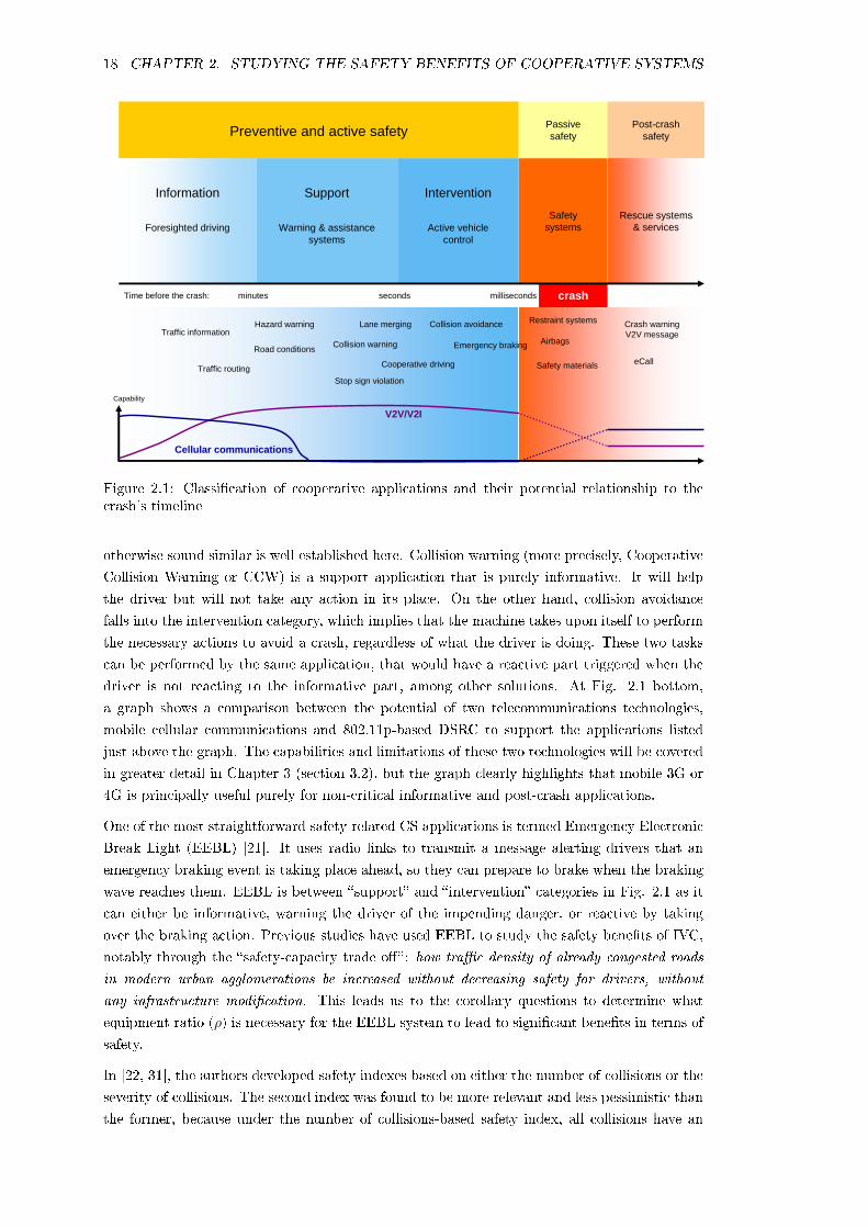
18 CHAPTER 2. STUDYING THE SAFETY BENEFITS OF COOPERATIVE SYSTEMS

crash

Preventive and active safetyPassive safety

Information

Foresighted driving

Support

Warning & assistance systems

Intervention

Active vehiclecontrol

Rescue systems& services

Safetysystems

Time before the crash: minutes seconds milliseconds

Traffic information

Traffic routing

Road conditions

Hazard warning Lane merging

Collision warning

Collision avoidance

Emergency braking

Cooperative driving

Stop sign violation

Airbags

Safety materials

Restraint systems

eCall

Crash warning V2V message

Post-crash safety

Capability

V2V/V2I

Cellular communications

Figure 2.1: Classication of cooperative applications and their potential relationship to thecrash's timeline

otherwise sound similar is well established here. Collision warning (more precisely, Cooperative

Collision Warning or CCW) is a support application that is purely informative. It will help

the driver but will not take any action in its place. On the other hand, collision avoidance

falls into the intervention category, which implies that the machine takes upon itself to perform

the necessary actions to avoid a crash, regardless of what the driver is doing. These two tasks

can be performed by the same application, that would have a reactive part triggered when the

driver is not reacting to the informative part, among other solutions. At Fig. 2.1 bottom,

a graph shows a comparison between the potential of two telecommunications technologies,

mobile cellular communications and 802.11p-based DSRC to support the applications listed

just above the graph. The capabilities and limitations of these two technologies will be covered

in greater detail in Chapter 3 (section 3.2), but the graph clearly highlights that mobile 3G or

4G is principally useful purely for non-critical informative and post-crash applications.

One of the most straightforward safety-related CS applications is termed Emergency Electronic

Break Light (EEBL) [21]. It uses radio links to transmit a message alerting drivers that an

emergency braking event is taking place ahead, so they can prepare to brake when the braking

wave reaches them. EEBL is between support and intervention categories in Fig. 2.1 as it

can either be informative, warning the driver of the impending danger, or reactive by taking

over the braking action. Previous studies have used EEBL to study the safety benets of IVC,

notably through the safety-capacity trade o: how trac density of already congested roads

in modern urban agglomerations be increased without decreasing safety for drivers, without

any infrastructure modication. This leads us to the corollary questions to determine what

equipment ratio (ρ) is necessary for the EEBL system to lead to signicant benets in terms of

safety.

In [22, 31], the authors developed safety indexes based on either the number of collisions or the

severity of collisions. The second index was found to be more relevant and less pessimistic than

the former, because under the number of collisions-based safety index, all collisions have an

2.2. LITERATURE REVIEW AND STATE-OF-THE-ART 19

equal impact whereas collisions at lower relative velocities typically lead to less severe injuries

and fatalities than collisions at higher velocities. Nonetheless, for both indexes, it was found

that IVC contributed to the increase in the string's safety. Lambert et al. [23] provided a more

in depth analysis of the equipment ratio inuence on the vehicle's string's safety. It remained

within the context of the safety index based on the total number of collisions; dierent models

for the distribution of inter-vehicular distances were studied. The study's simulation concluded

that only a small equipment ratio was necessary to drastically reduce the number of collisions.

For example, at a capacity of 3,000 vehicles/hour (a very dense trac) and ρ = 5%, the

number of collisions reduced by two third compared to an unequipped eet. The best results

were obtained with ρ = 25% , where the number of collisions was reduced by 90% (at higher

capacities) and remained very stable for most simulated capacities.

The question of the appropriate equipment ratio ρ is not trivial. Safety-orientated CS systems

have high theoretical benets [44], but nothing guarantees that these benets will be obtained

if the eet is heterogeneous. Takatori and Hasegawa [46] have shown that while CCW-equipped

vehicles might benet from positive eects within 20 and 60% of market penetration (the same

as ρ), those positive eects are really noticeable above 60% for the whole eet. However, simply

reaching ρ = 20% will take a certain amount of time, let alone 60%.

Let us have a simple simulation of the market penetration ρ of a given CS system. We have ymax

the number of years for which the simulation will run; N0 the initial eet size and Ntotal (y) the

eet size for any given year y; Nnew is the number of vehicles that are added to the eet each

year, which can be either the number of registrations, or the actual increase in size accounting

for scrapping; Neq (y) is the number of CS-equipped vehicle in year y; s is the ratio of equipped

vehicles on the rst year and i is the ratio of equipped vehicles within Nnew; nally, ρ (y) gives

the equipment ratio on a given year y. We assume that both Nnew and i are constant over the

timeframe of the simulation. The simulation is described by the following pseudo-algorithm:

First year (y = 1):

For 1 to N0

* Randomly generate Neq (y = 1) ≤ s×Ntotal CS-equipped vehicles

End for

Then ρ (y = 1) =Neq(y=1)

N0

Ntotal (y = 1) = N0

Following years (1 < y ≤ ymax):

For y = 1 to ymax

* Randomly generate P ≤ i×Nnew CS-equipped vehicles

* Then Neq (y) = P +Neq (y − 1)

* Ntotal (y) = Nnew +Ntotal (y − 1)

* ρ (y) =Neq(y)Ntotal(y)

End for

Note that this model is not accurate past a given value of ymax, , as the number of scrapped

vehicles is not modelled realistically and the eet increase (new registrations) is assumed to be

20 CHAPTER 2. STUDYING THE SAFETY BENEFITS OF COOPERATIVE SYSTEMS

0 2 4 6 8 10 12 14 16 18 200

10

20

30

40

50

60

Years after first deployment

% o

f eq

uip

ped

veh

icle

s in

th

e fl

eet

i = 10%i = 25%i = 50%i = 75%i = 100%

Figure 2.2: Simulation of market penetration (ρ) for an on-vehicle system

constant. Typically, this value would be about the same as the average lifespan of a modern

light vehicle i.e. 20 years. Let us have the following values [47]:

Nstart = 248.76× 106

Nnew = 16.0× 106

s = 0.05%

i = [10, 25, 50, 75, 100] %

ymax = 20

Fig. 2.2 shows the evolution of ρ for dierent values of i over 20 years. The fastest way to

reach ρ = 20%, is by having i set at 100% (i.e. imposing it on all new vehicles), where it would

only take 4 years. Achieving such a rate requires strong government leadership and a standard

that is accepted by all vehicle manufacturers in the world, which does not exist for most CS

applications at the moment. If all new vehicles are not equipped with the system, which is

more likely to be the case, the time to reach ρ = 20% increases signicantly. For example, if

i = 25%, after 20 years we will have ρ = 14%.

Without concerted eort, the market penetration rate will remain small. For example in 2002,

ACC was tted on 0.05% of the latest manufactured Toyota vehicles in the United States [32].

At this rate, only 1 in 1900 vehicles would be equipped taking 2006 years. The recent economic

crisis have also aected the deployment of such systems, with recent forecasts showing only

5.2 millions ACC-equipped vehicles in the world by 2015 , a meagre ρ = 0.52%. At such low

levels, the network eect syndrome [48] might hinder the system's deployment and acceptance

because quality of service is poor for early users, which would be especially true for systems

such as EEBL or CCW, that actively relies on other equipped vehicles to perform its tasks.

2.2. LITERATURE REVIEW AND STATE-OF-THE-ART 21

Thus, one must ensure that the system remains functional in heterogeneous environments (i.e.

at low values of ρ) and encourage its diusion among road users. From a marketing point of

view, Eichler et al. [49] suggested developing comfort-orientated V2I applications initially so

customers will be enticed to invest quickly in communication-capable vehicles. Approximately

after one decade, CS safety applications could be introduced into this more mature market, at

a higher initial market penetration rate. From a technical point of view, the system must be

developed to be robust in heterogeneous environments, what augmented perception could be

used to do.

2.2.3 Vehicles strings scenario(s)

Throughout this study, we will focus on a single scenario that we will use as our reference in

later chapters. Its generic name is vehicles strings scenario but there are many references to

it as the brick wall scenario [50]. Actually, the brick wall scenario is only one of two ways

the vehicles string scenario can be played out, and arguably the least realistic one. Overall, the

scenario is an emergency braking scenario involving a string of vehicles driving on a freeway

(see Fig. 2.3). The string's leader suers from a crash which triggers a series of rear-end crashes

in reaction as the following vehicles are progressively aected by the event. One can describe

a braking wave propagating through the string, which is a specic form of the kinematic wave

described by Lighthill and Whitham [51], which originally concerns variations of density inside

a vehicles string. In the brick wall version, the leader is stopped instantaneously (or almost) as

if it had collided a static heavy obstacle on the road, for an example, a collapsed overpass. In

the other more likely version, the leader performs a sudden emergency braking manoeuvre, still

moving some distance before coming to a complete stop. In both versions, the leader sends an

emergency collision warning message through IVC, thus performing an EEBL task. Vehicles

further down the string are able to use this information to respond to the crash.

Arguably, EEBL is the simplest form of safety-orientated CS application. Although it can

be argued that it is a primitive form of augmented perception, allowing vehicles to sense an

event that they normally cannot perceive, we will keep these two aspects of CS separate. Indeed,

EEBL will most likely be active for a very limited amount of time i.e. during an emergency

event, while augmented perception is more likely to be active at all times whenever a vehicle is

on the road, especially if it is used to support a road risk assessment application. Additionally,

it is not necessary to exchange complex information to be able to perform an EEBL task.

The amount of rear-end crashes that can be avoided using IVC depends on many parameters

including: the string's density, reaction times, IVC equipment ratio and the type of EEBL

application. In most cases, not all vehicles in the string can avoid the initial incident, so an

amalgam of crash vehicles tend to form at the beginning of the string. It has been shown

in[22, 31, 23] that the rst vehicle to avoid the crash will stop with a greater margin if there

are IVC-equipped vehicles in the string. This implies that, thanks to IVC, the minimal safe

vehicular interdistance can be reduced while maintaining overall safety for drivers in the string.

One limitation to this study, as it is usually applied to simulations, is that IVC-equipped vehicles

apply the brakes regardless of the driving context. It means that a secondary crashing incident

will occur a distance away from the leader vehicle. However, the number of collisions that might

have been avoided if no IVC was present did not undermine the safety benets of IVC [22].

It should be noted that the vehicles string scenario is limited to EEBL. Indeed, we will also

use it to evaluate augmented perception, where a more complex scenario will be considered

22 CHAPTER 2. STUDYING THE SAFETY BENEFITS OF COOPERATIVE SYSTEMS

Normal driving

CrashAlert message transmission

BrakingStopped vehicle

CollisionStopped vehicles

Figure 2.3: Four stages of the vehicles string scenario

for assessing crash risk for an individual vehicle, or for a group of vehicles. The vehicles

string scenario can be made as complex as required, from very homogeneous regularly-spaced

strings to heterogeneous ones where interdistances can uctuate. Incidentally, our CS simulation

architecture's objective is to be able to oer this large array of variability.

The rationale for choosing this scenario as our reference scenario for implementations and

simulations can be justied in several points:

Rear-end crashes represent between one fth and one third of all road crashes [29, 30]

and it is widely demonstrated that the majority of drivers do not follow safe interdistance

recommendations [3]. Thus, a system that can reduce rear-end crashes will contribute

signicantly to the reduction of road casualties.

Freeways are the least complex road environment, with driving ows well segregated and

a limited set of possible manoeuvres. Thus, they are the easiest to study and the simplest

to approximate in simulations or on test tracks.

Due to the reasons above, deployment of CS applications on freeways are expected to

be marketed before other road settings. Thus, EEBL and related cooperative safety

systems should be studied thoroughly so they can deliver their promises and be selected

by automotive manufacturers and regulatory authorities for commercial deployment.

The scenario is versatile enough to be used for studying simpler CS applications such as

EEBL, to more complex ones based on augmented perception.

The range of test tracks available at the Versailles-Satory grounds allows us to easily

deploy this scenario with actual vehicles.

2.3. STUDYING CS: SIMULATION VERSUS EMPIRICAL METHODOLOGIES 23

2.3 Studying CS: simulation versus empirical methodolo-

gies

In the introduction, we mentioned that the aim of this chapter is to select between two possible

research methodologies in studying the limitations of CS (and augmented perception) and

their expected safety benets. The nal research methodology should be the one that is most

likely to provide us with results on augmented perception's benets that are realist enough to

withstand scrutiny. It will have to provide conditions that are similar to the future conditions

into which the studied applications are likely to be deployed, as well as matching the conditions

of current applications within which they will be compared to. This means being able to provide

conditions that are similar to an open road driving environment, and that generates normal

and non-normal (i.e. dangerous) driving conditions.

Actually, there are three possible answers to this methodological question: advanced simula-

tions, theoretical studies and empirical implementation. Note that here, simulations cover a

large variety of potential methods. We will principally understand simulations in the context of

microscopic simulations of a number of vehicles in a simulated environment, equipped (or not)

with a specic system that is studied. Indeed, within the context of augmented perception,

large-scale trac simulations for example, have a too wide of a scope. Because of that, they do

not oer the necessary granularity required to study the performance of perception algorithms.

Some of the previous studies upon which our work is based have used theoretical approaches or

simple simulations to assess the safety benets of CS applications. However, we already men-

tioned that we aim at obtaining results that account for many potential imperfection sources.

In order to improve the results obtained by previous research, a theoretical analytical approach

would not allow obtaining realistic results without a signicant increase in complexity. The

large discrepancies between theoretical and measured IVC performance (see Chapter 3) are an

example of a theoretical methodology's limitations, as they would be too complex to model

analytically. For these reasons, we will consider that theoretical methods are out of this thesis'

scope.

Without further assumptions, these two methodological approaches cannot be discriminated. It

can be argued initially, that an actual empirical approach which uses on-road implementation

of the system to be studied, is better than the limited and non-complete reproduction that

would be proposed by a simulation. However, there are a number of advantages to simulation

[52], and it is possible to create meaningful and successful simulations, provided a number of

factors are taken into account and adjusted [53].

In Table 2.2 we propose a listing of simulation versus empirical methods in the context of

studying a CS application within a specic test scenario. The parameters in the scenario are

variables such as the number of vehicles and the type of driving manoeuvres that have to be

performed. Environmental factors such as the meteorological conditions and the surrounding

trac are considered independently. A number of unknown or uncertain a-priori quantities are

written in italics.

Table 2.2 shows that there is no methodology that has a clear advantage over the other, given the

unknown quantities that aect (mostly) the empirical methodology. The unknown quantities

are present within the context of research on CS. We need to determine which methodology is

the most appropriate in solving our research questions adequately, notably by evaluating the

impact on some potential issues in our research process.

24 CHAPTER 2. STUDYING THE SAFETY BENEFITS OF COOPERATIVE SYSTEMS

Table2.2:Compariso

nofsim

ulatio

nvs.

empirica

lmeasurem

ents

Simulatio

nEmpirica

lstu

dy

Varia

bility

ofthescen

ario

'sparameters

Neartotal

Importa

nt

May

require

complex

models

forsomeparameters

Migh

tbe

limited

bylogistica

landtim

ingissu

es

Contro

lover

thescen

ario

'sparameters

Total

Importa

nt

(inclu

dingmodicatio

ns)

Changes

inoneset

ofparameters

migh

thave

hidden

consequ

ences

onothers

Migh

tbe

limited

bylogistica

landtim

ingissu

es

Enviro

nmentalfacto

rsEasy/quick

tochange

Cannotbemore

realistic

thanrea

lityLess

represen

tativ

e(approx

imatio

n)

Canbelim

itedbyunavaila

bility

ofappropria

temodels

More

complex

toobtain

thedesired

conditio

ns

(variab

leweather,

etc.)Lack

ofcontro

lonsomefacto

rsCanbedi

cultto

measu

resomevaria

bles

Acco

untin

gim

perfectio

ns

Know

nmodelisa

tionandpossib

ilityto

vary

their

sources/

magnitu

de

Immediate

(noadditio

nalwork

need

ed)

Require

complex

models

ifrea

lismmust

beensured

(more

prep

aratio

nwork)

Canbelim

itedbyunavaila

bility

ofappropria

temodels

Lim

itedcontro

lover

allim

perfectio

nsources

Di

culty

todiscrim

inate

each

imperfectio

nsources

Outco

me's

represen

tativ

eness

Noidenti

edadvantage

Actu

alsystem

(orprototype)

used

Lim

itedto

theaccu

racy/delity

ofthemodels

used

Lim

itedbythesca

leofthestu

dyortheenviro

nment

(closed

road)

Humanfacto

rsNoidenti

edadvantage

Immediate

acco

untin

gCannotacco

untforallHF

(sensitiv

ityto

limita

tionsofdrivers'

models)

Migh

thave

hidden

orunwarra

nted

inuence

onthe

scenario

outofsco

pe

Repeatability

Easy

torep

eatlargeamountoftim

esNoidenti

edadvantage

Less

varia

bility

betw

eeneach

iteratio

ns,dependingon

themodels

used

Migh

tbe

complica

tedby

HF/logistics/

lack

ofdesired

env.

facto

rs

Scaleofstu

dy

Largesca

lespossib

leNoidenti

edadvantage

Migh

tbe

heavy

interm

sofworkloa

dto

implem

ent

large

study

Scaleofstu

dystro

ngly

limited

byava

ilablereso

urces

Logistics

andcost(s)

Lim

itedcosts

andlogistics

Noidenti

edadvantage

Inappropria

teprocessin

gpow

ermightlen

gthen

implem

entatio

nofstu

dy

Highter

costs

when

more

thanafew

vehicles

involved

Complex

logistics

(ndingdrivers,

insta

lling

equipment,etc.)

2.3. STUDYING CS: SIMULATION VERSUS EMPIRICAL METHODOLOGIES 25

As evident in the literature review, the vehicle strings scenario has been investigated within

a simulation to show the safety benets of using IVC inside the strings. We have noted a

number of limitations surrounding these previous works, notably in terms of the assumptions

used to model IVC (notably the 802.11p-based ones). Even if the simulation's assumptions

allow demonstrating the benets of IVC, especially in small increment ratios, these limitations

may preclude the scenario's transposition to actual vehicles strings. Indeed, communication

latency could negate the observed positive eects, for example a large latency in transmitting

the emergency message would not give drivers enough time to improve their reaction to the

braking event. The IVC technology used therefore has to ensure that latency remains under a

certain threshold. On the other hand, previous simulations assumes perfect (i.e. instantaneous

and lossless) communications. Other strong assumptions are taken by previous simulations,

notably concerning the vehicles composing the string and their drivers. The string is seen as

perfectly homogeneous, and the drivers perfect (they are constantly at their best reaction times

and do not make interpretation errors). Variations in vehicles and drivers characteristics could

have the same negative eects on the simulations' results.

Evaluating the impact of the imperfections from the expected benets of the IVC is important.

We note that the empirical research methodology allows us to take into account all the imme-

diate potential limitations that can be encountered by an IVC system. The advantages and

disadvantages of simulation (for our research) have already been addressed in these previous

studies. Given the absence of practical information in some categories and the availability of ap-

propriate resources (hardware, drivers, etc.) at the LIVIC laboratory, evaluating the empirical

methodology appears to be the most logical choice to start our research process. Furthermore,

the LIVIC laboratory had a set of simulation tools that could be modied and enhanced to

accommodate our research needs which allowed us to test if the other methodology could be

used successfully. This in return, meant avoiding locking ourselves into a single methodology

from the beginning. This process should allow lling in the gaps and lead to a more informed

choice.

To do so, we will implement our reference vehicles string scenario. The experimentation will have

two related goals. Firstly, it will have to validate the methodology, characterise its limitations

and provide evidence it will be possible to use it for further research. In order to satisfy

this future research objective, the second goal to this on-tracks implementation will be to

determine whether it is possible to validate IVC benets in an imperfect environment, compared

to the homogeneous strings and environments available in simulations. Indeed, performing

an empirical measurement study with a set of IVC-equipped vehicles in a realistic driving

environment is a good way to test several issues concurrently.

A number of benets can be expected from the empirical Methodology. This approach allows

taking into account all possible imperfections that can arise inside a real driving environment,

including but not limited to IVC ones. Additionally, using real drivers and vehicles allow

introducing heterogeneity in the string. Note that the focus of this experiment is not on

human factors, such as drivers' reaction time, although being able to measure some driver-

related metrics is a consequence of the experimental design. However, human factors have been

identied as part of the issue that might negatively aect the study, so being able to take them

into account, up to a limit, is to our advantage.

In the following sections, we will present the design and implementation of a scenario aimed at

fullling these goals. The direction of this thesis will be contingent on our experience with the

implementation and discussed in the nal section (4.5).

26 CHAPTER 2. STUDYING THE SAFETY BENEFITS OF COOPERATIVE SYSTEMS

2.4 On-tracks demonstration of EEBL

We reiterate the two major goals from this implementation:

1. Validate the use of an empirical research methodology for future CS-related research and

identify its weaknesses.

2. Conrm previous research on the contribution of IVC to the safety of vehicles strings.

These goals are inter-related because achieving the second goal means that a fully empirical

methodology focused on implementing actual devices on vehicles, can be used for the remainder

of this thesis. On the other hand, if the second goal is not achieved or is not satisfactory, a fully

empirical methodology would not be the most informed choice. In that case, advanced simu-

lations which can be enhanced by empirical research, would be the most appropriate approach

to assess the safety benets of CS.

2.4.1 Design and experimental protocol

2.4.1.1 Experimental requirements

To verify the potential safety benets of our EEBL application, we need to compare the number

of crashes before and after the introduction of the EEBL system. This is done by counting vir-

tual collisions (see ??) at dierent values of equipment ratio and compare the collision counts'

variation to match it with the simulation results; the overall variation has to be compared

rather than the absolute number of collisions. Experimental requirements are:

Requirements concerning the environment

The environment in which the experiment will take place must:

Be similar to the driving conditions found on a freeway, at least for a few hundred metres.

.

Allow enough driving distance for drivers to form an appropriate string.

Be a closed (private) environment to avoid disturbance from trac.

Requirements concerning the EEBL system

The EEBL system which will be used for the experiment must:

Be inexpensive, using mostly pre-existing hardware so that they are not too far away from

future commercial applications.

Use a common hardware and software architecture for all vehicles and/or RSUs (Road

Side Units).

Allow complete control over the software suites, so that all parameters can be known and

edited if required by the experimental protocol.

Have an HMI (Human-Machine Interface) that can be used to convey emergency inform-

ation to the drivers.

2.4. ON-TRACKS DEMONSTRATION OF EEBL 27

Requirements concerning the experimental protocol

The experimental protocol used for the experiment must:

Have at least 4 vehicles forming a string and braking in safe conditions, while still allowing

a virtual crash.

Have dierent models of vehicles present in the string.

2.4.1.2 Participants

The implementation requires the participation of a number of drivers to drive the vehicles

engaged in the string. Since the aspect of human factors is not our concern, recruiting the

drivers was straightforward. Volunteers from the LIVIC laboratory were gathered from age 25

to 57 , roughly 3/4 male versus 1/4 female. Overall, 8 individuals including the author took part

in the experiments including preliminary tests, over several days.

The drivers were each given a vehicle and which equipment with the EEBL system was determ-

ined beforehand. They start to drive and are instructed to form a string and maintain, as best

they can, the relative interdistances between each vehicle (which have been selected beforehand,

for example 20 metres). Visual clues on the road, or stickers on the vehicles' windshields are

used to enhance the sense of relative distances. The drivers are also instructed to brake when

the EEBL system's HMI displays an alert symbol, which is triggered by the receipt of an emer-

gency braking message over the IVC device. If driving in an unequipped vehicle, the driver has

to brake when the leading vehicle is braking, as would happen in a real string. This introduces

a delay in the braking reaction, compared to equipped vehicles.

This protocol is repeated a number of times with each drive labelled a run. The order of

drivers in the string is changed regularly.

2.4.1.3 Procedures

The experimental scenario is designed to reproduce previous simulations' conditions as closely as

possible, which is a single-lane vehicles string, with a controlled repartition of the interdistances

between each vehicle. A number of procedure parameters must thus be considered; string

size, equipment ratio (ρ), distribution of equipped vehicles, interdistances, and speed of the

vehicles. As the scenario aims at reproducing an emergency situation that would lead to rear-

end crashes, precautions must be taken to safeguard drivers (and research hardware) from risks,

while allowing for meaningful results to be obtained. To do so, a method to obtain virtual

collisions must be designed. Note that this subsection provides a number of justication for

choices of procedures. Indeed, the aforementioned parameters must be carefully tuned if the

experimental results are to be compared to previous simulations. Otherwise, the simulations

and the present implementations would be too dierent from each other.

Virtual collisions and safety considerations The scenario requires vehicles to brake in

order to avoid impeding head-on collisions, but it is not possible for them to actually collide.

The benets of IVC are shown from the decrease in collision count according to ρ. The best

way to apply this to an actual implementation, without putting drivers into conditions that

28 CHAPTER 2. STUDYING THE SAFETY BENEFITS OF COOPERATIVE SYSTEMS

would lead to real collisions, is counting virtual collisions as one would count actual collisions

in a vehicle string on a freeway. Virtual collisions are simply events emulating real collisions,

which are safe for drivers.

The best analogy to an emergency-braking vehicles string that we have found involves using

an alternating formation (see Fig. 2.4). With vehicles positioned alternatively on two lanes,

the interdistances between vehicles Vi and Vi+1 can be maintained at the required value while

the actual distance between two vehicles in the same lane is twice the interdistance. Vi and

Vi+1 can then virtually collide during the braking manoeuvre, which is measured when their

longitudinal position intersect.

However, dense strings might actually negate the security oset gained by using this formation.

Thus, it is necessary to compute a safety margin that bounds the possible interdistances in

the string. The residual distance dr between two vehicles after braking in the same lane can

be computed with equation 2.1., where di is the pre-braking interdistance, v is the vehicles'

velocity and τ is the (following) driver reaction time.

dr = 2× (di − vτ) (2.1)

With τ = 0.8 seconds, an interdistance of 30 metres becomes unsafe at 110 km/h and 20

metres becomes unsafe at 75 km/h. Considering that drivers will have diculties knowing the

interdistances precisely, especially given the alternating formation, additional safety margins

might have to be implemented. This limits the achievable speed/interdistances combinations

(see Table 2.3).

The alternating formation also has some limitation:. since vehicle Vi driver is able to see vehicle

Vi+2 brake lights, it is probable that its reaction time will be modied compared to a normally

organised string where Vi+1 obstructs the view to Vi+2.

Counting virtual collisions in the alternating formation, as well as obtaining back-up information

in case the virtual collisions approach does not work, requires measuring the following variables:

The location of vehicles when they have stopped, which determines if a virtual collision

took place.

The interdistance between vehicles, both to help with counting crashes and to know the

string's density just before the braking event.

The latency in the EEBL warning, that includes the communication latencies and pro-

cessing latencies associated with the application, such as decoding the warning message,

interpreting it and displaying the information to the driver through a HMI.

The drivers' reaction time(s).

To measure the vehicle's location and interdistances, we used a dual-head laserscanner that is

located on the side of the road. It is positioned and orientated so that there is no occultations

by the vehicles, especially in the braking area. This sensor is also useful to record the driver's

reaction time, as it can accurately sense the vehicle's behaviour so, using speed and position

data we can estimate the moment the vehicle starts to slow down. To do so, the laserscanner

has to be synchronised with the telecommunication system, and the reaction time measurement

will always include the braking system's reaction time in addition to the driver's. The latency

2.4. ON-TRACKS DEMONSTRATION OF EEBL 29

dinter,0;1dinter,1;2V0V1V2

Virtual first vehicle

RSUSensor trafficcone 1

2

Figure 2.4: Implementation scheme with the alternating formation for a safe experiment andthe virtual leader vehicle

is measured within the on-board EEBL system, which ensures that all the vehicles (and the

roadside laserscanner) are synced throughout the experiment. Further details are provided in

the following section on how these systems were implemented.

Number of vehicles in the string and IVC equipment We limited ourselves to a max-

imum of ve research vehicles for practical reasons. This limited the results' achievable granu-

larity, but a larger number of vehicles would have required complex logistics, especially in terms

of drivers, which we did not have access to. The ve vehicles were sucient in order to study

the eects of IVC on the string's safety. The vehicles used were:

two identical Renault Clio III 5-door estates (nicknamed Tic and Tac 3)

one Renault Scénic I 5-door compact MPV (nicknamed VIPER)

one Citroën C4 Grand Picasso 5-door MPV.

one Peugeot 307 5-door hatchback.

The vehicles were tted with powered equipment racks in the boot and several in-cabin screens

for the HMI. A variety of sensors can be tted on them depending on the experimental re-

quirements; one of the Clios had a permanent forward-facing radar, the Senic had multiple

laserscanners, cameras and a forward-facing radar for a complete perception of its surround-

ings, and the Peugeot 307 is also equipped with two laserscanners and cameras for stereovision.

However, none of this equipment was used in our implementation, which only required a com-

munication device (see 2.4.2).

The goal is to test the scenario at each value of ρ: 0/5 (unequipped string), 2/5 (leader + 1

follower), 3/5, 4/5, and 5/5; or in terms of percentage: 0, 40, 60, 80 and 100%. Equipped vehicles

are randomly distributed in the string, based on drawings of an uniform probability law. Data

from [23] suggests that the most important reduction in crash numbers occurs when ρ rises from

0 to 30%. At rst, it seemed that we would not be able to study what is going on between 0 and

40%, indeed ρ = 20% corresponds to just one equipped vehicle in a ve-vehicle string. If the

leader is considered an equipped vehicle, there is no receptor vehicle left for ρ = 20%. However,

to avoid this limitation, our implementation used a workaround where the leading vehicle is

virtualised and replaced by an RSU that sends a emergency message at the appropriate time

(more details on the setting in 2.4.2).

3Tic & Tac are the French name of Disney's Chip and Dale

30 CHAPTER 2. STUDYING THE SAFETY BENEFITS OF COOPERATIVE SYSTEMS

Table 2.3: Interdistances computed from speed and capacity. Capacity in vehicles/hour, velocityin kilometres/hour and interdistance in metres

Velocity50 70 90 110 130

Capacity1800 23.78 34.88 46.00 57.12 68.222000 21.00 30.99 41.00 51.01 61.002500 16.00 23.99 32.00 40.00 48.003000 12.67 19.33 26.00 32.67 39.33

Interdistances and vehicle speed The interdistances between vehicles is the next major

factor that will inuence the number of crashes in the string. In [22] interdistances are modelled

as constants noised by a centred Gaussian noise; whereas in [23]three models are used constant,

exponential and truncated (strictly positive) Gaussian distributions. The road capacity, the

temporal denition of the string's density, was the principle parameter in previous studies.

However, in an experimental application of the vehicles string scenario, capacity is not an

appropriate indicator. By controlling the string's average intervehicular distance, it is possible

to approximate simulated capacities. The average interdistance d and road capacity c are linked

as shown in equation 2.2, where v is the string velocity and l is the average vehicle's length [51]:

c =v(

l + d) (2.2)

LIVIC's eet l is 4.002 metres; using this value we can compute the interdistances required, at a

specic speed, to approximate a given capacity value (see Table 2.3). For example, if the string

velocity is 90 km/h and the desired equivalent capacity is 2,000 vehicles per hour, the average

interdistance must be 41 metres. These values represent the ideal target interdistances, but it

can be dicult for drivers to maintain this without visual clues or technological help (with a

forward facing radar, for example). As mentioned above, drivers are provided with visual clues

in the form of stickers on their windshields however, these measures only allow a relatively rough

following of the appropriate interdistances. Additionally, to accurately record the interdistance

before and during the emergency braking event, we used the roadside laserscanner.

2.4.2 Implementation and measurements setup

To implement the EEBL scenario, we developed an IVC warning system architecture, which

is shown in Fig. 2.5. It is organised in 3 blocks (represented by the dashed boxes) which are

each located on a separate platform vehicles, the RSU and the sensor cone. As also shown in

Fig. 2.4, the RSU and sensor cone are used to simulate the string's rst vehicle that broadcast

the warning message. The vehicle's setup (labelled IV on the gure, for Intelligent Vehicle),

is reproduced in each equipped vehicle. Most of the hardware used here is a precursor to

the hardware used for the experiments performed in Chapter 3, in which more details will be

provided regarding the implementation of IVCD (including 802.11p). In the present chapter,

we will only mention the major interest point of how the hardware and software were designed

for this experiment.

The RSU and IV blocks use identical hardware and software. An eBOX638 embedded com-

puter hosts all applications (running under Linux) and is connected by Ethernet networking

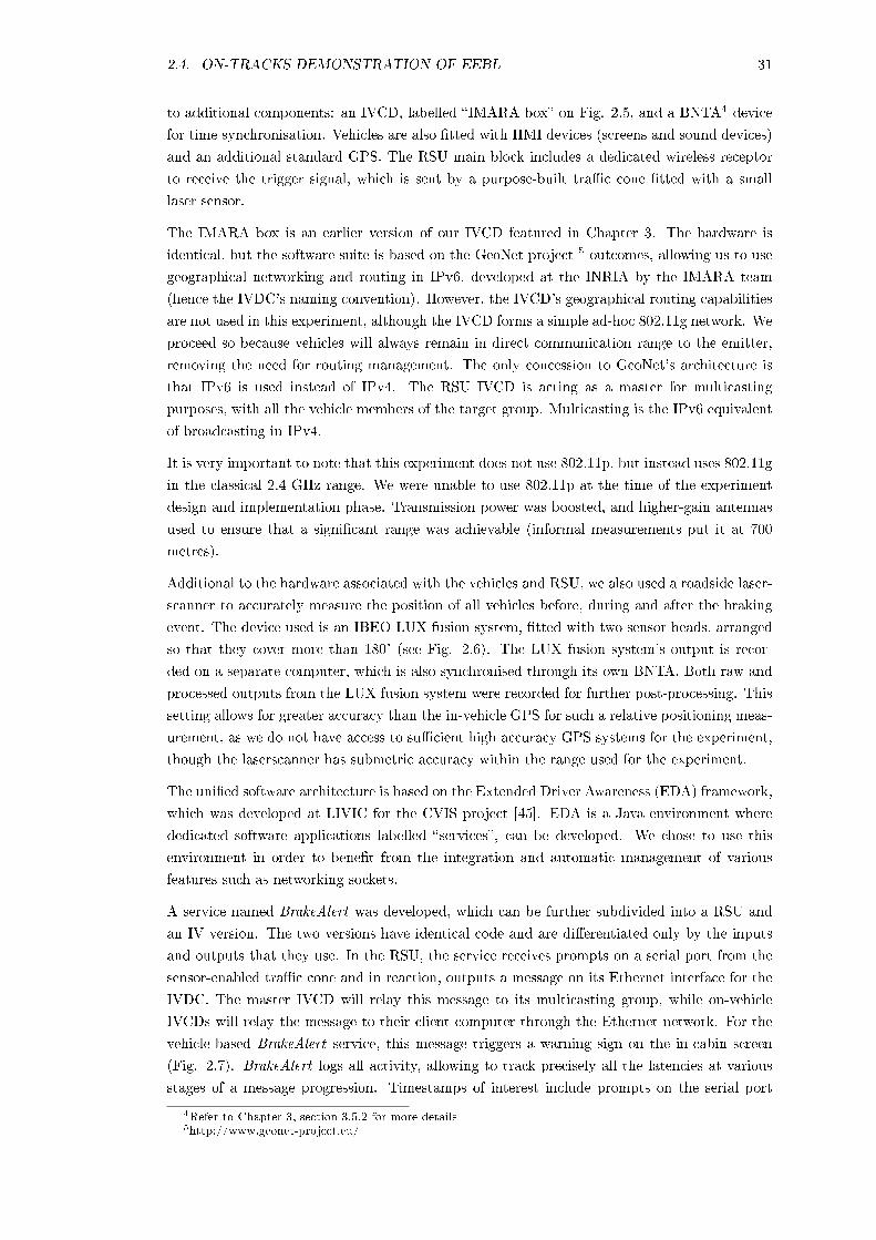
2.4. ON-TRACKS DEMONSTRATION OF EEBL 31

to additional components: an IVCD, labelled IMARA box on Fig. 2.5, and a BNTA4 device

for time synchronisation. Vehicles are also tted with HMI devices (screens and sound devices)

and an additional standard GPS. The RSU main block includes a dedicated wireless receptor

to receive the trigger signal, which is sent by a purpose-built trac cone tted with a small

laser sensor.

The IMARA box is an earlier version of our IVCD featured in Chapter 3. The hardware is

identical, but the software suite is based on the GeoNet project 5 outcomes, allowing us to use

geographical networking and routing in IPv6, developed at the INRIA by the IMARA team

(hence the IVDC's naming convention). However, the IVCD's geographical routing capabilities

are not used in this experiment, although the IVCD forms a simple ad-hoc 802.11g network. We

proceed so because vehicles will always remain in direct communication range to the emitter,

removing the need for routing management. The only concession to GeoNet's architecture is

that IPv6 is used instead of IPv4. The RSU IVCD is acting as a master for multicasting

purposes, with all the vehicle members of the target group. Multicasting is the IPv6 equivalent

of broadcasting in IPv4.

It is very important to note that this experiment does not use 802.11p, but instead uses 802.11g

in the classical 2.4 GHz range. We were unable to use 802.11p at the time of the experiment

design and implementation phase. Transmission power was boosted, and higher-gain antennas

used to ensure that a signicant range was achievable (informal measurements put it at 700

metres).

Additional to the hardware associated with the vehicles and RSU, we also used a roadside laser-

scanner to accurately measure the position of all vehicles before, during and after the braking

event. The device used is an IBEO LUX fusion system, tted with two sensor heads, arranged

so that they cover more than 180° (see Fig. 2.6). The LUX fusion system's output is recor-

ded on a separate computer, which is also synchronised through its own BNTA. Both raw and

processed outputs from the LUX fusion system were recorded for further post-processing. This

setting allows for greater accuracy than the in-vehicle GPS for such a relative positioning meas-

urement, as we do not have access to sucient high accuracy GPS systems for the experiment,

though the laserscanner has submetric accuracy within the range used for the experiment.

The unied software architecture is based on the Extended Driver Awareness (EDA) framework,

which was developed at LIVIC for the CVIS project [45]. EDA is a Java environment where

dedicated software applications labelled services, can be developed. We chose to use this

environment in order to benet from the integration and automatic management of various

features such as networking sockets.

A service named BrakeAlert was developed, which can be further subdivided into a RSU and

an IV version. The two versions have identical code and are dierentiated only by the inputs

and outputs that they use. In the RSU, the service receives prompts on a serial port from the

sensor-enabled trac cone and in reaction, outputs a message on its Ethernet interface for the

IVDC. The master IVCD will relay this message to its multicasting group, while on-vehicle

IVCDs will relay the message to their client computer through the Ethernet network. For the

vehicle-based BrakeAlert service, this message triggers a warning sign on the in-cabin screen

(Fig. 2.7). BrakeAlert logs all activity, allowing to track precisely all the latencies at various

stages of a message progression. Timestamps of interest include prompts on the serial port

4Refer to Chapter 3, section 3.5.2 for more details5http://www.geonet-project.eu/

32 CHAPTER 2. STUDYING THE SAFETY BENEFITS OF COOPERATIVE SYSTEMS

Figure 2.5: General system's architecture

2.4. ON-TRACKS DEMONSTRATION OF EEBL 33

Figure 2.6: Map of the scenario's area of interest, on the eastern straight part of la routière;the laserscanner coverage area is shown to scale

Figure 2.7: Warning message as displayed on the EDA human-machine interface

of the RSU, transmission of outbound messages to the Ethernet interface, arrival of inbound

messages at the Ethernet interface and activation of the HMI. Some data are not accessible:

(1) any latency within the trac cone to RSU chain and (2) latencies inside and between

the IVCDs. The second limitation occured because we did not have control over the INRIA's

software, which was a strong incentive to implement an open source system as described in

Chapter 3.

Eventually, the scenario was performed on the eastern straight part of la routière track, as

shown in Fig. 2.6. The drivers form the string over the rst part of the 800 metres section,

then press the brakes within the laserscanner's coverage area. Even with allowing more room,

the speed track is impractical because the laserscanner does not have a large-enough eld of

view. The braking event triggered a small delay after the rst vehicle drove pass the sensor

cone. The drivers were instructed to perform emergency braking as soon as the emergency

message displayed on their HMI or, if they are in an unequipped vehicle, as soon as they see the

brake lights on the car driving in front of them in the side line. In an unequipped string, the

leading driver was instructed to press the brakes at their convenience when they have passed

the trac cone.

34 CHAPTER 2. STUDYING THE SAFETY BENEFITS OF COOPERATIVE SYSTEMS

Figure 2.8: Latencies recorded for 113 messages

2.5 Results

The scenario was undertaken in late 2010, over a three-day experimental session with a total of

24 full runs using 4 vehicles. We considered these measurements to be a half-size demonstration

of a future experiment involving eight vehicles. The goal was to validate our implementation

and also, more importantly, to test whether the experimental protocol was workable. Although

there were no objections to the experimental protocol beforehand, the design process had shed

some doubts as to whether we would be able to obtain meaningful results. However, these

doubts could not be laid to rest without actually taking the system to the track.

The 24 test runs (and a number of secondary runs) showed that our architecture and imple-

mentation are functional, as well as demonstrating how implementing an EEBL scenario can

be done. All the variables were measured successfully, with the vehicles driving at 70 km/h

and the chosen target interdistance was 25 metres. The most immediate useful ndings in the

EEBL application concerned latency. We measured the whole latency, from the BrakeAlert

RSU application to the BrakeAlert IV application and not just the IVC latency. As already

stated, the host application does not send the message. A dierent device, the IVCD, is re-

sponsible for doing so. As such, there is an increased latency due to the time necessary for the

IVCD in receiving the message from the host (through Ethernet), process it and send it to the

wireless chipset. This process is repeated in the receptor IVCD. Our latency measurement must

thus be understood as the worst case scenario for an implementation that uses modems, i.e.

specialised devices to manage networking needs.

113 messages were suitable for analysis (a single multicast generated more than one data point).

The average delay was 46 milliseconds, although 11% of the messages were delayed by more

than 100 milliseconds; the most extreme latency was measured close to 600 milliseconds (see

Fig. 2.8). All measurements were taken at ranges less than 150 metres, as the rst vehicle had

already passed by the RSU. Some of the drivers involved reported that in extreme cases, the

delay was noticeable. 46 milliseconds is not a very large delay, however the exchanged frame is

2.5. RESULTS 35

relatively small, similar to the ones that will be used in the 802.11p experiments (see Chapter

3). Although we found that using IPv6 added a small amount of delay, the principal reason

for these large values seem to be the multiple number of processes that needed to take place

between the two applications. Having no control over the IVCDs, we were not able to verify

these delays. Nonetheless, these latency measurements are useful to set a benchmark for our

subsequent 802.11p performance evaluation, as improving latency is deemed to be one of the

most important improvements enabled by the amendments to the 802.11p.

For the measurement of interdistances and braking patterns, typical results obtained from the

roadside laserscanner sensor are shown in Fig 2.9, this particular example having three vehicles

with ρ = 0. Fig. 2.9a shows the progression of each vehicle along the track's longitudinal axis

over time (transversal position is irrelevant here); g. 2.9b shows the speed of each vehicle, over

the same time frame. The three vehicles' formation is clearly visible, as well as the braking

event.

An analysis of these positioning measurements allows us to extract the drivers' reaction time .

The average reaction time computed from the laserscanner data for these same ten test drives is

606 milliseconds, which is quicker than the average reaction time in more generic conditions [54].

When comparing the average reaction time for two consecutive vehicles between test drives with

and without BrakeAlert, the average value decreases from 606 to 378 milliseconds. However,

there are not enough measurements to claim that the modied and non-modied averages

are statistically signicant. Nonetheless, it is a logical result resulting from outcomes of the

experiment and drivers' feedback. Furthermore, it can be expected that all vehicles would brake

within a brief window after receiving the warning message, with varying timeframes depending

on the time needed for drivers to become aware and reaction to the HMI warning. The present

data does not allow us to determine if this is the case or not.

On the other hand, it became evident during the 24 test runs that obtaining virtual collisions was

very dicult. For example, over 10 test drives using 4 vehicles and without any communications,

we only received 2 virtual collisions and 2 close calls in conditions that in previous simulations

would have led to a crash. Our assessment of this result is that in these experimental conditions,

human factors take an importance that we had not anticipated beforehand.

The drivers are strongly expecting the braking event, as they were aware of the goal of the

test runs from the start. Understandably, it was impossible, for safety reasons, to conduct

a blind experiment especially given the relatively small number of drivers that were involved

in this test. The aim of this study was not to assess a driver's reaction time or any other

human-related metrics rather, we were more interested in designing an engineering-orientated

experiment with a focus on the system's performance. Because of these conditions, the drivers'

reaction times were considerably decreased. This is pointed out by the fact that some drivers

noticed the slow warning message, which demonstrates they were highly aware of what was

going on. Furthermore, all the vehicles used for the test runs are recent models capable of

strong emergency braking. These two eects compounded to reduce the number of virtual

crashes by making emergency stops very ecient.

Eventually, we discovered an important IVCD-related limitation. Having no control over the

IVCDs, we were not able to analyse precisely the IVCD's functions and any latency this could

add to our system. No actual EEBL application would function in such a way and it is obvious

that 10% of latencies over 100 milliseconds is not acceptable in any safety critical applications.

36 CHAPTER 2. STUDYING THE SAFETY BENEFITS OF COOPERATIVE SYSTEMS

(a) Vehicle positions along the longitudinal axis of the test track

(b) Vehicles' speed

Figure 2.9: Laserscanner measurements for a three vehicles string, showing the braking event

2.6. CONCLUSION 37

2.6 Conclusion

The aim of this chapter is to settle on a choice between two possible research methodologies

regarding the evaluation of performance and safety benets of Cooperative Systems in general

and augmented perception, in particular. The two potential methodologies are (1) advanced

simulations, or (2) actual fully on-road implementation in a research setting. A-priori, none

of the two competing methodologies are superior to the other, although we identied a lack of

information regarding the empirical methodology's merits and some disadvantages.

Thus, given logistical factors and research interests at the time, we selected the empirical

research methodology for initial evaluation, and implemented an EEBL application on Satory's

test tracks. This implementation had two related goals; (1) validate the use of an empirical

research methodology for future CS-related research (and identifying its weaknesses) and (2)

empirically conrming previous research on the contribution of IVC to the safety of vehicles

strings. Indeed, showing that we could obtain results on IVC/CS safety benets would have

validated the use of a fully empirical research methodology. If that was not the case, advanced

simulations would be a more appropriate choice, with the possibility of enhancing them through

specialised empirical research.

The results obtained from the implementation are mixed. Although the engineering aspects

were challenging, we found no major diculty in designing an EEBL application for several

vehicles, and putting them on the track. Important benchmark data were obtained from the

IVC using IEEE 802.11g. The implementation also allowed us to gather useful engineering

experience that will be applied for the data collection described in Chapter 3. On the other

hand, it highlighted a number of issues with the empirical approach. The logistics proved to

be more complex than expected, even for a relatively simple experiment such as EEBL. More

importantly, issues with the drivers meant that we were unable to obtain the virtual collisions

that was our prime interest in validating the safety benets of IVC in such an empirical setting.

Accordingly, we can ll-in the table from section 2.3, presenting in Table 2.4 an updated version

(changes shown in bold font).

Taking these results and the related methodological limitations in consideration, we have come

to the conclusion that it is unwarranted to continue with this EEBL implementation and a

full empirical research methodology. A research methodology focused on advanced simulations

appears to be the best course of action to follow, whether in validating and improving previous

studies on IVC safety benets, or preparing the evaluation of augmented perception. Indeed,

using advanced simulations at this stage enables a much wider eld of research and experi-

mentation than keeping a focus on on-road systems. It also allows us to get around logistical

issues that may be associated with implementing a system to a scale where it starts to yield

relevant outcomes (this is one of the reasons for large multinational projects such as CVIS or

COOPERS). It will also help alleviate the human factors-related issues that became apparent

during the EEBL implementation.

Settling for a simulation-focused methodology does not mean that simulations are perfect.

There is signicant room for improvement in their design and the models used to represent

important parameters of CS-related research. Consequently, improving the simulation envir-

onment of CS to provide more realistic and accurate studies will be the focus in the following

chapters.

The enhancements will concern technical aspects of CS, most notably the simulation of IVC.

38 CHAPTER 2. STUDYING THE SAFETY BENEFITS OF COOPERATIVE SYSTEMS

Table2.4:Compariso

nofsim

ulatio

nvs.

empirica

lmeasurem

ents

Simulatio

nEmpirica

lstu

dy

Varia

bility

ofthescen

ario

'sparameters

Neartotal

Importa

nt

May

require

complex

models

forsomeparameters

Limited

bylogistica

landtim

ingissu

esContro

lover

thescen

ario

'sparameters

Total

Importa

nt

(inclu

dingmodicatio

ns)

Changes

inoneset

ofparameters

migh

thave

hidden

consequ

ences

onothers

Limited

bylogistica

landtim

ingissu

es

Enviro

nmentalfacto

rsEasy/quick

tochange

Cannotbemore

realistic

thanrea

lityLess

represen

tativ

e(approx

imatio

n)

Canbelim

itedbyunavaila

bility

ofappropria

temodels

More

complex

toobtain

thedesired

conditio

ns

(variab

leweather,

etc.)Lack

ofcontro

lonsomefacto

rsCanbedi

cultto

measu

resomevaria

bles

Acco

untin

gim

perfectio

ns

Know

nmodelisa

tionandpossib

ilityto

vary

their

sources/

magnitu

de

Immediate

(noadditio

nalwork

need

ed)

Require

complex

models

ifrea

lismmust

beensured

(more

prep

aratio

nwork)

Canbelim

itedbyunavaila

bility

ofappropria

temodels

Lim

itedcontro

lover

allim

perfectio

nsources

Di

culty

todiscrim

inate

each

imperfectio

nsources

Outco

me's

represen

tativ

eness

Noidenti

edadvantage

Actu

alsystem

(orprototype)

used

Lim

itedto

theaccu

racy/delity

ofthemodels

used

Lim

itedbythesca

leofthestu

dyortheenviro

nment

(closed

road)

Humanfacto

rsNoidenti

edadvantage

Immediate

acco

untin

gCannotacco

untforallHF

(sensitiv

ityto

limita

tionsofdrivers'

models)

Presen

ceofhidden

orunwarra

nted

inuences

onthescen

ario

andexperim

entalprotocol

Repeatability

Easy

torep

eatlargeamountoftim

esNoidenti

edadvantage

Less

varia

bility

betw

eeneach

iteratio

ns,dependingon

themodels

used

Complica

tedbyHF/logistics/

lack

ofdesired

env.facto

rsScaleofstu

dy

Largesca

lespossib

leNoidenti

edadvantage

Migh

tbe

heavy

interm

sofworkloa

dto

implem

ent

large

study

Scaleofstu

dystro

ngly

limited

byava

ilablereso

urces

Logistics

andcost(s)

Lim

itedcosts

andlogistics

Noidenti

edadvantage

Inappropria

teprocessin

gpow

ermightlen

gthen

study'sim

plem

entatio

nHighcosts

when

more

thanafew

vehicles

involved

Complex

logistics

(ndingdrivers,

insta

lling

equipment,etc.)

2.6. CONCLUSION 39

Our goal will be to allow representing realistic imperfection within these simulations, as they

are the factors that will aect any CS application performance the most. Although we chose

to focus on the simulation research methodology, this does not mean that there will be no

more on-road studies for the remainder of this thesis. On the contrary, we will show that using

empirical data is necessary in improving the quality of CS simulations. Indeed, as we will

see in the following chapter, there is an important need to study the empirical performance

of telecommunication technologies poised to support CS, most notably 802.11p. An empirical

model of 802.11p performance metrics aimed at simulations of CS applications, rather than

focusing on the network performance, is the type of improvement that we are proposing.

This work is necessary, as it will provide a solid research environment that will enable answering

two of the research questions mentioned in Chapter 1, i.e. (1) can an augmented map-based

risk assessment system be more ecient than a non-cooperative similar system? and (2) what

are augmented perception limitations, given current technology in embedded computing and

telecommunications?

Summary of the chapter's contributions

Outcomes

A research methodology focusing on improving the realism of CS simulation, includ-

ing empirically-driven improvements, was selected.

The technical feasibility of an EEBL implementation was demonstrated.

Engineering guidelines were set for further on-road performance analysis.

Performance benchmarks for latency in 802.11g IVC were obtained.

Limitations

Human factors and experimental protocol issues did not allow a study into the safety

contributions of IVC into a vehicles string.

40 CHAPTER 2. STUDYING THE SAFETY BENEFITS OF COOPERATIVE SYSTEMS

Chapter 3

Evaluation of telecommunications

for augmented perception

3.1 Introduction

In the previous chapter we experimented with an actual implementation of a Cooperative

Systems application (EEBL), with mixed results which lead to the conclusion that it was more

appropriate to focus on enhancing simulations of CS applications to study their limitations

and their safety benets as our research methodology. To start this enhancement process,

the present chapter focuses on the underlying technology supporting Cooperative Systems i.e.

telecommunications.

CS, and augmented perception, claim to be useful in reducing the number of fatalities on the

road, as we saw in the literature review in Chapter 2. But, one must be able to demonstrate

they can indeed live up to their promises. Telecommunications are used to extend a system's

perceptive horizon and provide additional information that are expected to have important

safety benets. Before even asking how it is possible to use cooperation to enhance road users'

safety, this augmentation of information source begs the question; what are augmented percep-

tion's limitations, given current technology in embedded computing and telecommunications?

This is one the main research question that will be addressed by this thesis. Indeed, one can

argue that inecient intervehicular communications may render the benets from introducing

information sharing null. Accordingly, the rst step in evaluating the limitations of augmen-

ted perception, in general, and augmented maps in particular should focus on the principal

technological dierence between themselves and non-cooperative perception.

Thus, the aim of this chapter is, rstly, to evaluate the telecommunications (specically 802.11p)

performance and its ability to deliver appropriate quality of service to support safety-critical

applications. Then, our second aim is to create a new representative empirical model of limited

complexity, that will be used to support and enhance (with empirical data) our subsequent

higher-level simulations development (e.g. an augmented map building architecture), that we

will explain in the following chapters.

Performance evaluation of 802.11p is an ongoing area of research, but we will show that the

state-of-the-art neglects some important performance metrics (principally latency). This justi-

es undertaking a series of new, controlled data collections that allows the assessment of the

42 CHAPTER 3. TELECOMMUNICATIONS FOR AUGMENTED PERCEPTION

performance metrics which are the most relevant to CS. Our evaluation process allowed us to

dene a set of boundaries on the performance that one can expect from 802.11p. It showed

that many assumptions behind CS's road safety benets have been too optimistic, expecting

802.11p to achieve theoretical performances in most cases. Our measurements show that this is

not the case. This also relates to the existing simulation of 802.11p, which work upon unrealistic

performance assumptions.

The dichotomy between theoretical and experimental performance is further aggravated by the

fact that we performed our measurements in a relatively open and controlled environment, and

not on actual roads, where sources of imperfections are omnipresent. It means that actual

on-road performance might be even more degraded than what we measured. Nonetheless, our

measurements do not discount the use of telecommunications to enhance perception. Rather,

they advise being careful about quality of service assumptions when designing higher-level safety

applications.

We then proceed to develop an empirical model for 802.11p performance metrics. The state-of-

the-art in empirical modelisation of 802.11p shows that models usually focus either on higher

layers of the OSI architecture, more relevant to information dissemination in vehicular networks,

or either on the actual physical layer. Our requirements are intermediate, as we are solely

interested in the performance metrics for a vehicular network where complex routing is not

necessary. Also, we did not nd a model that included an evidence-based simulation of latency

in 802.11p for this type of small network that we are interested in. The aim of building this

model is to support and enhance higher-level simulations of CS applications with up to a

dozen road actors. The proposed model has several advantages, such as taking into account

environmental factors such as the weather, as well as performance variations introduced by

hardware inhomogeneities.

Chapter outline

The rst section reviews V2V/I telecommunication technologies in general, and IEEE 802.11p

in particular. It exposes our research context, and argues that an empirical performance eval-

uation of telecommunications systems is essential to design ecient, potentially safety-critical

CS. At rst, we present details on telecommunications within CS in general, detailing the ex-

isting technologies and tackling issues such as scalability and data security. Then, we focus on

technologies from the IEEE 802.11 family, detailing how they have already been used in CS.

We then present the specics surrounding 802.11p. The state-of-the-art in 802.11p performance

evaluation is explained; limitations of existing studies are discussed to highlight the rational for

our own evaluation process. Eventually, existing empirical models of 802.11p are presented, to

oer some context regarding and to present the rationale for creating our own model.

The second and third sections present our experimental design, from the measurement scenarios

to the hardware and software architectures. We explain the rationale for the design, and what

is and is not possible to study.

The fourth section analyses the results from the data collection undertaken on the Satory's test

tracks (closed roads), allowing it to dene a set of boundaries on the performance that one can

expect from 802.11p. The considered performance metrics are latency, frame loss, and range.

We provide evidence that previous expectations in terms of the possible 802.11p performance

have largely been over-optimistic, especially with the connection ranges that 802.11p systems

could achieve, even in relatively open freeway-like environments.

3.1. INTRODUCTION 43

The fth section then details the development of an empirical 802.11p performance model based

on the measurements detailed in the previous section. We present a two-step model building

process, starting with a simple polynomial approach before settling on the nal modelisation.

Eventually, in the nal section, we conclude on the limitations for 802.11p that have emerged

from the previous sections. We argue that researchers working on safety-critical CS should be

aware of these limitations, especially for their impact on augmented perception.

44 CHAPTER 3. TELECOMMUNICATIONS FOR AUGMENTED PERCEPTION

3.2 Literature review

3.2.1 IVC: the backbone of Cooperative Systems

Wireless Inter-vehicular Communications are the core of Cooperative Systems, as they provide

the link between the various actors in the cooperation environment. Because of their mobile

and highly variable nature, IVC impose new concepts for communication systems, information

dissemination and data security management. The term communication medium will be used

henceforth to describe all the processes involved in an Open System Interconnection (OSI )

type of telecommunication architecture see Fig. 3.1). Indeed, CS design covers all the aspects

of the OSI model, from the upper application layer to the lowermost physical layer (i.e. the

nature of the support medium, either radiofrequencies, infrared, etc.). However, we will exclude

the applications themselves from the communication medium: applications are data sources or

clients for the medium, but not an integral part of the medium itself. We shall note that the

present thesis will not cover each layer of the OSI model; we will look at, rstly, the lowermost

levels, and then place ourselves outside of the communication medium by focusing on the

application layer. It is however necessary to keep in mind design issues associated with these

lower layers, as they might inuence the upper layers.

Eichler et al. [49], Nagel et al. [55] provide a comprehensive list of the communication medium's

fundamental requirements, classied into two themes: (1) scalability, topology and routing;

and (2) data security. Nagel et al. [55] actually places an emphasis on one CS application,

cooperative driving, but the requirements listed for this specic application also applies to all

other cooperative applications. Before focusing on our core interest for this chapter, the physical

layer, we will provide a concise presentation of these requirements.

3.2.1.1 Scalability, topology and routing

One of the most fundamental requirement is that the IVC medium must not be aected by

scale eects, i.e. it must be fully scalable. It means that the medium must perform with

the same eciency regardless the number of communicating actors, as well as whatever the

extent of their geographic dispersion. For example, in a dense trac scenario, if the number

of communicating vehicles is large, broadcasting techniques such as ooding are at stake with

issues such as interferences, data packet collisions and major latency; this phenomenon is usually

described as a broadcast storm [56, 57]. Nagel et al. pointed out the need to minimise

latency with appropriate information dissemination techniques. They mentioned pre-allocated

frequencies or temporal windows as a possible solution (FDMA, TDMA), but this would require

a centralised architecture (server/client), which is not necessarily the most suitable architecture

for the quickly changing context of IVC (see below). Eichler et al. [49] also proposed not to use

broadcast but more sophisticated techniques such as power level control or beamforming. These

latter techniques are also important in managing interferences at smaller scales and limiting

the load on the communication medium.

Typically, the IVC medium's topology will be highly variable: the nodes' positions change

constantly, their numbers change as new vehicles enter the IVC range and others drive away,

links between the nodes change, etc. This volatile nature increases the required sophistication of

information dissemination techniques (especially if one wants to maintain high data security).

In this type of variable topology, classical routing and dissemination techniques faces some

3.2. LITERATURE REVIEW 45

Data unit Layer Function7 - Application Network process to applications

6 - Presentation

Data representation, encryption & decryption, convert machine-dependant data to machine-

independent data5 - Session Inter-host communication

Segments 4 - TransportEnd-to-end connections and

reliability, flow control

Packets 3 - NetworkPath determination and logical

addressingFrame 2 - Data link Physical addressing

Bit 1 - Physical Media, signal and binary transmission

OSI Model

Data unit

Media layers

Host layers

Figure 3.1: Layers of the OSI model

problems. For example, a ooding dissemination can saturate the network (creating a broadcast

storm); targeted complex techniques, such as unicasting, will increase data latency as well as

data overhead (which can lead to even more latency by increasing sizes of the frames) [49].

Higher level protocols, such as the TCP/IP internet suite, are also not necessarily appropriate

for a variable medium and will require modications.

Nagel et al. proposed to compensate these issues by building networks where each node (i.e.

each vehicle) would have an accurate knowledge of the network's topology, at all times. This

is a form of geographical routing (geo-routing). By modelling the network as an oriented

graph, incorporating all important parameters on each node (including data on the vehicle's

motion), links states and capabilities, one could use more optimised dissemination techniques.

Nodes would keep their information up to date by periodically broadcasting information on their

motion and state. The authors also envisioned a network topology evolution prediction stage.

However, this approach would be limited in regards to long-range communications, because

each node must have a limit to the extent of its knowledge of the network's topology.

Similar geo-routing techniques such as the Greedy Perimeter Stateless Routing (GPSR) or

Reactive Location Service (RLS) are described in [58]. The European GeoNet project1 has de-

veloped a standardised approach, using IPv6, that features geo-casting to specic geographical

zones, linked together by long-range communications over the Internet. Another solution pro-

posed by Cenerariol et al. [57] is to take into account the relevance of a piece of information via

an evaluation of the distance between the receiving node and the event described by this piece

of information. Thanks to this approach, a vehicle will not relay a message that is not relevant

to itself, contrary to a simple ooding scenario, thus limiting the load on the communication

medium.

We must emphasise here that routing and information dissemination issues are not, usually,

related to issues regarding the physical medium. We will not take further interest to these

former issues in this thesis, focusing solely on physical-layer related research problems.

3.2.1.2 Security

In the future, securing the communication medium will be indispensable, notably to provide

guaranteed quality of service and ensure that cooperative systems are well accepted by the

1www.geonet-project.eu

46 CHAPTER 3. TELECOMMUNICATIONS FOR AUGMENTED PERCEPTION

general public [49, 59]. Cooperative applications must have complete condence in the integrity

of the data they receive. This requires using cryptographic techniques to ensure malicious

messages are not transmitted on the network. Unfortunately, most of the current cryptographic

techniques appear to be un-adapted to the conditions of IVC. For example the classic technique

of public key infrastructure (PKI) is organised around a centralised architecture and cannot be

used in a decentralised network without modications. One of the modications could be the

elliptical curves cryptography described in [55]. Füÿler et al. [58] also notes that a certicate

system to verify a message content is not appropriate in an environment where nodes are unlikely

to meet each other more than once in their lifetime

Furthermore, it is important to ensure that the security of the medium does impact the propaga-

tion speed of data, that is, introducing additional latencies. Decrypting a message is not instant-

aneous, especially in cases where bilateral communications have to be used to exchange keys.

Füÿler et al. [58] found up to 50 milliseconds of additional latency introduced by cryptographic

processing.

3.2.2 A variety of Physical layers

So far, we have not considered the question of the exact technology that will be used to deploy

and support IVC, the physical layer in the OSI model. Ideally the communication medium

can be multi-supported in the future; that is using several dierent technologies at the same

time to carry information. This can be seen in the CALM framework2, which allows a variety

of technologies at the physical layer. Nevertheless, we have found that many current studies

usually focus on a single technological approach. Multi-support approaches are usually found

when inexpensive equipment is desired or if one support is used to conrm the information

carried by another. We have examples such as the combination between IEEE 802.11p and

802.15.4 in [60], looking into reducing the system's costs, and between infrared and Zigbee

(802.15.4-2003) in [61], using one technology to verify identication based upon the other. Fig.

3.2 shows a diagram of all types of physical supports for CS currently being considered.

The most popular, and likely to remain the most ubiquitous medium for intervehicular commu-

nications are radiofrequencies technologies, especially the IEEE 802.11 standards family. This

popularity is exemplied by the publication of an amendment (802.11p) to the IEEE 802.11

standard specically for CS usage (the complete version is found in [27]). Given the popularity

of this technology, and that this chapter will cover empirical evaluation of 802.11p, we will

address both in further detail respectively in section 3.2.3 and 3.2.4.

Other forms of radiofrequencies are also considered or already actively used: mobile phone

protocols such as GSM or UMTS; dedicated short-range technologies such as RFID or IEEE

802.15.4 (Zigbee, WirelessHART, etc.); terrestrial radio. The choice to use one form over

another is usually dictated by the pre-existence of an infrastructure network. Mobile phone

networks for example have the advantage of a widespread deployment (in France) or at least

inhabited (in Australia) areas. Focusing on using them, we can mention the German project

2CALM (Communication Access for Land Mobile) is an integrated architecture supporting communicationmedia and application diversity, and allowing many dierent communication scenarios (V2X, multihop, point-to-point and multipoint). Its goal is to provide an architecture that standardises the set of air interface protocolsand parameters for medium and long range, high speed IVC, using any of several communication media andnetworking protocols. This process should enable transparent connectivity over any possible medium. It hasbeen implemented in the EU through the CVIS project, inter alia.

3.2. LITERATURE REVIEW 47

Figure 3.2: Diagram presenting all the potential physical supports that are considered for CSdeployment

Aktiv CoCar [62] that uses Vodafone's UMTS network to send safety alerts, emergency vehicles

and trac information messages to vehicles via a central server [63].

However pre-existing networks have not been designed and built for automotive applications;

this means that they are not necessarily adapted to their requirements. One of the principal

issues with cellular networks is latency [64]. Because of the way telephone networks are built,

there is no direct communication possible between two nearby vehicles: the message they want

to exchange must transit through a number of routing systems rst. This means that cellular

networks are not suitable for time-critical message dissemination, such as required in CCW

applications, for example.

3.2.3 The IEEE 802.11 standard

IEEE 802.11 is a set of standards for implementing Wireless Local Area Network (WLAN)

radiofrequency communication, in the 2.4, 3.6 and 5 GHz frequency bands. It covers the MAC

and PHY layer of the OSI model. The original version of the standard was released in 1997

but is obsolete today. 802.11 started to be used commercially in 1999 with the formation of

the Wi-Fi alliance to market 802.11a and 802.11b. It has since grown tremendously for private

and public usage, with the advent of versions g and n, among others. For example, 13% of the

total internet usage in the United Kingdom went through Wi-Fi hotspots in 2011 [65]. In Table

3.1, we show a list of the dierent versions of 802.11 as well as several technical characteristics

pertaining to them.

Although it grants a degree of mobility, to laptops and smartphones on a university campus

for example, 802.11 was essentially developed for short-range, indoor usage with a focus on

high data rate (see Fig. 3.3). Indeed, no technology can compete with Wi-Fi in terms of

network capabilities for relatively static usage. However, this means that using 802.11 versions

to support the highly mobile telecommunications required in CS is not a straightforward choice.

Nonetheless, it was made because of the ubiquity of 802.11 technology and the fact that it oered

48 CHAPTER 3. TELECOMMUNICATIONS FOR AUGMENTED PERCEPTION

Table3.1:Tech

nica

lcharacteristics

of802.11versio

ns

Versio

nFreq

uency

band

(GHz)

Bandwidth

(MHz)

Maximum

data

rate

(Mbits/

s)Modulatio

nApprox

imate

indoor

range(m

etres)Approx

imate

outdoor

range(m

etres)

802.11

2.4

20

2DSSS,FHSS

20

100

802.11a

3.7

and5

20

54

OFDM

35

120(at5GHz)

or5,000

(at3.7

GHz)

802.11b

2.4

20

11

DSSS

35

140

802.11g

2.4

20

54

OFDM,DSSS

38

140

802.11n

2.4

and5

20or40

72.2

(with

20MHzbandwidth),

150(w

ith40

MHzbandwidth)

OFDM

70

250

802.11p

5.9

10

27

OFDM

N/A

1000

3.2. LITERATURE REVIEW 49

Wi-Fi

WiMAX

GSM

HSPA

UMTS

Speed

Mobility0.4 Mbit/s

600 Mbit/s(802.11n)

70 Mbit/s

15 Mbit/s

30 km20 km5 km< 1 km

Figure 3.3: Data rate (speed) versus mobility of wireless systems: Wi-Fi, WiMAX, HighSpeed Packet Access (HSPA), Universal Mobile Telecommunications System (UMTS) and GSM.Range and data rate are indicative and can vary depending on the conditions surrounding thedevice.

several advantages compared to competing mobile technologies, such as 3 or 4G connections.

Indeed, the latter require a SIM card to connect to the cellular network, which usage is not free.

More importantly, they suer from important latency issue as they form a centralised network;

for example, even in good signal conditions and with small packets, the latency (as the Round

Trip Time) will be in the 100 to 300 milliseconds in 3G networks [64]. WiMAX (included

in IEEE 802.16) is a complementary system to 802.11, that is designed for metropolitan area

network with a 50 km radius. It can support a higher degree of mobility than the classic 802.11

versions, but it has certain requirements (notably in terms of access points) that make it less

adaptable for highly-mobile ad-hoc networks. Thus, 802.11 is perceived as the best available

technology to oer capabilities for decentralised, ad-hoc and free networking.

Since interest in CS started in the late 1990s, many studies have assessed 802.11b or 802.11g

capabilities for cooperative applications. We will quote a few of these studies, but it is important

to state that earlier versions of 802.11, or versions that are primarily dedicated to indoor usages,

have mostly been discontinued for cooperative applications on the road. This is especially true

ever since the 802.11p amendment was dened, which was designed specically for high-mobility

vehicular use. We have not found any ongoing research that still uses non 802.11p versions.

A number of performance evaluation have investigated performance metrics such as range,

bandwidth and latency in 802.11b/g networks for CS applications. An interesting study can

be found in Ammoun et al. [66], Ammoun [48], who measured 802.11g performance in urban

and rural environments. In dense urban environments, namely the sixth district of Paris, range

varied from 120 to 320 metres; in rural environments they reached up to 500 metres. In [67], the

maximum range was 850 metres, yet the actual useful range was less than 200 metres (for an

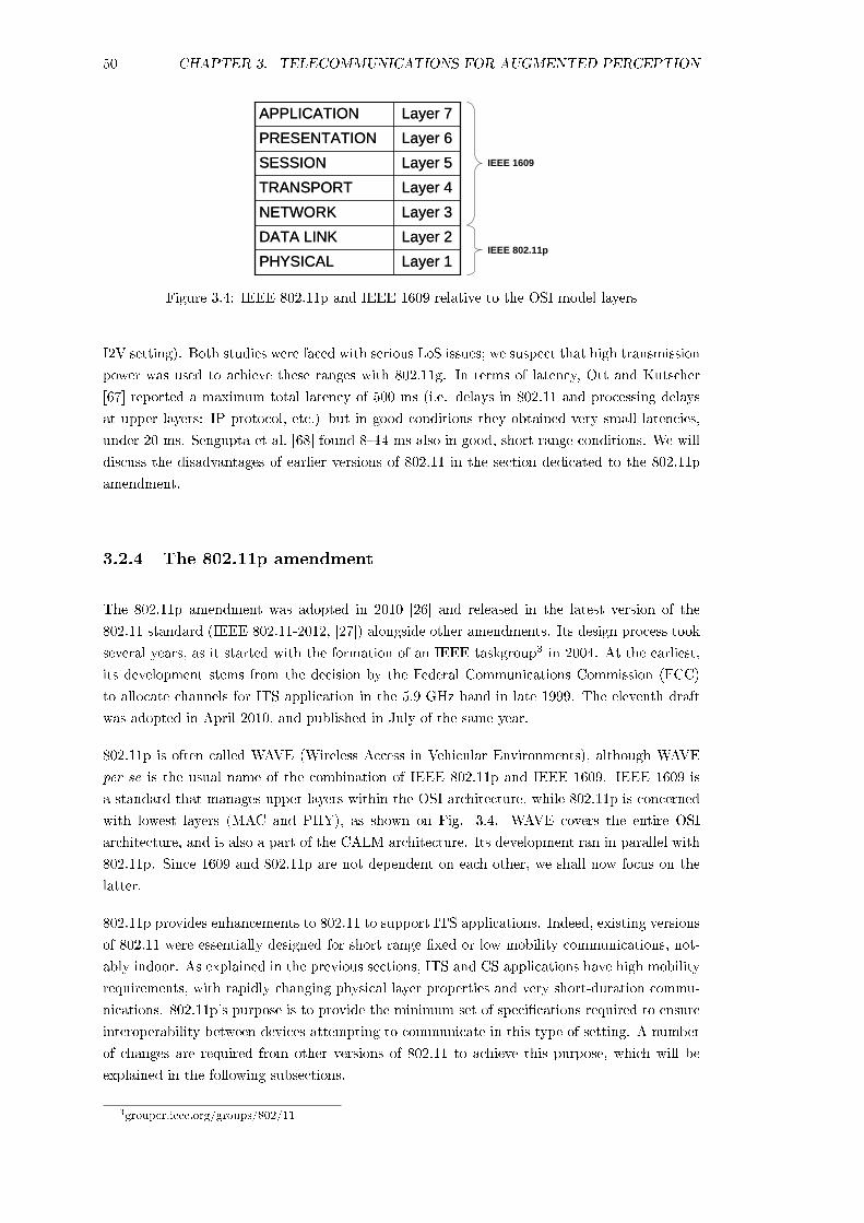
50 CHAPTER 3. TELECOMMUNICATIONS FOR AUGMENTED PERCEPTION

Layer 1PHYSICAL

Layer 2DATA LINK

Layer 3NETWORK

Layer 4TRANSPORT

Layer 5SESSION

Layer 6PRESENTATION

Layer 7APPLICATION

Layer 1PHYSICAL

Layer 2DATA LINK

Layer 3NETWORK

Layer 4TRANSPORT

Layer 5SESSION

Layer 6PRESENTATION

Layer 7APPLICATION

IEEE 802.11p

IEEE 1609

Figure 3.4: IEEE 802.11p and IEEE 1609 relative to the OSI model layers

I2V setting). Both studies were faced with serious LoS issues; we suspect that high transmission

power was used to achieve these ranges with 802.11g. In terms of latency, Ott and Kutscher

[67] reported a maximum total latency of 500 ms (i.e. delays in 802.11 and processing delays

at upper layers: IP protocol, etc.) but in good conditions they obtained very small latencies,

under 20 ms. Sengupta et al. [68] found 814 ms also in good, short range conditions. We will

discuss the disadvantages of earlier versions of 802.11 in the section dedicated to the 802.11p

amendment.

3.2.4 The 802.11p amendment

The 802.11p amendment was adopted in 2010 [26] and released in the latest version of the

802.11 standard (IEEE 802.11-2012, [27]) alongside other amendments. Its design process took

several years, as it started with the formation of an IEEE taskgroup3 in 2004. At the earliest,

its development stems from the decision by the Federal Communications Commission (FCC)

to allocate channels for ITS application in the 5.9 GHz band in late 1999. The eleventh draft

was adopted in April 2010, and published in July of the same year.

802.11p is often called WAVE (Wireless Access in Vehicular Environments), although WAVE

per se is the usual name of the combination of IEEE 802.11p and IEEE 1609. IEEE 1609 is

a standard that manages upper layers within the OSI architecture, while 802.11p is concerned

with lowest layers (MAC and PHY), as shown on Fig. 3.4. WAVE covers the entire OSI

architecture, and is also a part of the CALM architecture. Its development ran in parallel with

802.11p. Since 1609 and 802.11p are not dependent on each other, we shall now focus on the

latter.

802.11p provides enhancements to 802.11 to support ITS applications. Indeed, existing versions

of 802.11 were essentially designed for short range xed or low mobility communications, not-

ably indoor. As explained in the previous sections, ITS and CS applications have high mobility

requirements, with rapidly changing physical layer properties and very short-duration commu-

nications. 802.11p's purpose is to provide the minimum set of specications required to ensure

interoperability between devices attempting to communicate in this type of setting. A number

of changes are required from other versions of 802.11 to achieve this purpose, which will be

explained in the following subsections.

3grouper.ieee.org/groups/802/11

3.2. LITERATURE REVIEW 51

3.2.4.1 Changes compared to 802.11abg/n

802.11p species several changes from other versions of 802.11. It is similar to 802.11a in most

aspects, with changes made ensuring its usefulness within the ITS context [69].

The principal dierence between the common 802.11bg/n and 802.11p is the frequency band

occupied, 2.4 and 5.9 GHz respectively (see section 3.2.4.2 for regulatory questions). In that

respect, 802.11p is similar to 802.11a, which operates at 5 GHz. Operating at higher frequen-

cies has several advantages such as less interference and higher bandwidth (because of greater

spectrum availability), higher data rate and smaller antennas. Surprisingly for an outdoor

application, operating at higher frequencies also means that the achievable range for a same

transmission power is slightly lower (path loss is proportional to the square of the frequency,

and absorption by solid objects is higher). Nonetheless, modulation techniques and antenna

design can compensate such issues.

802.11p features 10 MHz-wide channels, spaced 10 MHz apart, while other versions have 20

MHz-wide channels spaced 5 MHz apart. Thus, there is minimal channel overlap in 802.11p

compared to other versions, and the RMS delay spread 4 is oset by using smaller channels

[70].

The other major innovation introduced by 802.11p is its ability to function outside of the normal

(in 802.11) ad-hoc framework. In the 802.11 architecture, the basic building block of a LAN is

the Basic Service Set (BSS). In infrastructure mode, the most common Wi-Fi in households is

a single access point together with all associated stations called a BSS; the access point acts as

a master to control the stations within its BSS.

The other mode is the ad-hoc mode, where it becomes possible to create a LAN without a

controlling access point; this network is called an Independent Basic Service Set (IBSS). This

mode is the most logical to use with Vehicular Ad-hoc Networks (VANETs), as it accounts for

mobility issues by greatly reducing the length of procedure that is required for a new station to

connect to the network. However, authentication and association still happens for an IBSS,

which can incur some delays. Since the 802.11p amendment's purpose is to allow communication

between devices in rapidly changing settings, where some data exchange must be completed in

time frames much shorter than the minimum possible with BSS or IBSS networks, it makes

sense that it includes provisions for functioning outside of their context.

802.11p allows a device that is not a member of a BSS to transmit data frames, outside the

context of said BSS, in what is called the OCB mode (Outside the Context of a BSS, not

to be confused with the Oset Codebook Mode in cryptographic block ciphers). This type of

communication is only possible between devices that are able to communicate directly over the

wireless medium, and thus takes place at the lower MAC level. Regulatory authorities require

that it takes place on specic channels to avoid interfering with BSS or IBSS activities. OCB

mode allows immediate communication, avoiding the latency associated with establishing a

BSS. Applications are numerous, for example the fast dissemination of critical safety alerts or

the exchange of data between two vehicles driving in opposite directions on the freeway, where

relative speed is more than 250 Km/h. However, a device functioning in OCB mode cannot

join a BSS or an IBSS, so it is unwarranted for it to operate in this mode at all times, unless

4The delay spread is usually the dierence between the time of arrival of the earliest signicant multipathcomponent (LoS component) and the time of arrival of the latest multipath component; it is largely increasedin real outdoor environments because of the high number of potential sources for multipath eects.

52 CHAPTER 3. TELECOMMUNICATIONS FOR AUGMENTED PERCEPTION

the entire communication architecture is designed around it. Switching the OCB on and o is

controlled by a ag, dot11OCBEnabled.

Some issues remain with the new amendment; most importantly the high-mobility context is

still a source of problem and a signicant research question. For example, the question of how

on-vehicle devices should share the radio resources to ensure service quality, remains unresolved,

as 802.11p uses Distributed Coordination Function (DCF): DCF was originally designed for low

mobility networks [71].

3.2.4.2 Regulatory context

The expected performance advantage in the 5.9 GHz band was not the only reason that sup-

ported moving away from the 2.4 GHz band. Indeed, the latter band has become, over the

past decade, quite crowded with other users and parasite broadcasts, especially in urban areas:

private, public and corporate Wi-Fi networks and hotspots, Bluetooth systems, radars, mi-

crowave ovens parasite emissions, etc. This is mostly due to the fact that operations in the 2.4

GHz band are mostly unlicensed, which oers no protection against interference to a particu-

lar user or system. Although this profusion of existing networks could be potentially turned

to the ITS's advantage, such as in [40] where it is used to provide continuous connectivity to

infotainment applications, in most cases it is more of a disadvantage than an advantage. This

is especially true if one considers the problem of delaying critical safety messages.

The 5.9 GHz band is a less crowded part of the spectrum, where parasitic emissions are less

likely. However, it would be untrue to claim that the 5.9 GHz band is completely unused.

International-level regulation by the International Telecommunication Union (ITU) has alloc-

ated frequencies blocks of the 5.9 GHz. Earth-to-space and space-to-Earth communications by

satellite operators are the principal licensed uses of this band; notably, the 5.850-5.925 GHz

band is used for Earth-to-space non-mobile links in all the 3 ITU regions (region 1 includes the

EU, region 2 includes the USA and region 3 includes Australia and Japan).

Since Earth-to-space communication is largely directed, and occurs only at a limited number of

locations, other unlicensed usage is permitted in the band, as long as transmission power does

not exceed a certain threshold. Authorised usage vary depending on the regions: in region 2

(USA) amateur usage and radiolocation are allowed; in region 3 (Australia) only radiolocation

is allowed. Fixed or mobile ground-to-ground communications are allowed in the three regions,

and include 802.11a as a part of the industrial, scientic and medical (ISM) band.

In order to secure spectrum usage and limit interferences with other systems, regulatory au-

thorities have specied that the ITS band can be used by licensed operators only. Within the

ITU provisions, each regional and national regulatory authority is allowed to further specify

authorised spectrum usage, and manage licensing issues. This means that dierent spectrum

allocations and licensing options exist for the ITS band.

As of mid-2012, from the three major worldwide automotive industry centres, only Japan has

not nalised its spectrum allocation. The FCC in the USA, and the ETSI in the European

Union have both allocated to the ITS band the whole of the 5.850-5.925 GHz frequency range,

with 10 MHz-wide channels. The FCC has designed 7 channels, while the ETSI created only

5 and reserved two additional for future use. A comparison of the European and American

spectrum allocations is shown in Fig. 3.5; the gure also shows the maximum transmission

power (or Eective Isotropically Radiated Power, EIRP) authorised for each channel. For

3.2. LITERATURE REVIEW 53

example, European regulations allow an EIRP of 33 dBm in all channels, approximatively 2

Watts. Note that the 5.850-5.925 GHz band in the European Union does not have a Dynamic

Frequency Selection5 (DFS) requirement, unlike the close 5.470-5.725 GHz band, which is used

primarily for on-vehicle radar operations, but also allows WLAN operations.

Service channel (mixed use)Safety only channelNon-safety channel

Control channelFuture use

Frequency (MHz) 5850 5855 5860 5865 5870 5875 5880 5885 5890 5895 5900 5905 5910 5915 5920

USAMax EIRP (dBm)

EUMax EIRP (dBm) 33

33 43 23 40

Figure 3.5: Spectrum allocations and EIRP limits in the USA and EU

The Japanese spectrum allocation plan diers from the other two as it was initially planned for

the 5.770-5.850 GHz band. However, Japan's regulatory authority has not nalised its decision

yet, and observers expect that to allow interoperability, it will extend its allocation plan to the

band chosen by the USA and Europe.

Australia has not made a decision on its exact spectrum allocation and licensing options for the

ITS band, as the Australian government is still waiting for the major automotive manufacturing

regions to settle their allocation plans. Some overlaps do exist, such as the frequencies used by

the police in the state of Victoria that overlaps with the ITS band starting from 5.875 GHz and

up. Typically, police and ITS communications would take place in a similar context and range,

which means they are likely to interfere with each other if both usage are authorised.

3.2.4.3 State-of-the-Art: performance evaluation of 802.11p

Prior to 2008, 802.11p was primarily evaluated in theoretical and simulation studies. Empirical

evaluation was limited to 802.11a, because of the similarity between the two standards, although

a number of researchers continued to use 802.11g to work on CS. Starting in 2008, 802.11p

hardware became available in prototype and, later, commercial forms. This enabled the actual

eld evaluation of 802.11p performance using the amendment's complete specications, rather

than approximation with 802.11a (or other versions).

Theoretical and simulation studies of 802.11p abounds. A large number of them use simulators

from the ns-x family6, which grant the user a wide array of possibilities in terms of model

development for the whole 802.11p architecture. As a result, such studies vary widely in scope

and interests. For example Yang et al. [72] and Torrent-Moreno [73] studies geographical routing

strategies to disseminate safety-critical messages in freeway trac with minimal loss, using

agging or contention area approaches respectively. Sepulcre and Gozalvez [74] highlighted how

vehicle behaviour could aect 802.11p ability to transmit critical message in time, proposing

to adopt schemes such as adaptive power control and opportunistic transmission rates. Böhm

and Jonsson [75] looked into the issue of handover between roadside units, proposing a MAC

improvement to reduce handover delays and maintain appropriate quality of service (QoS) for

5Dynamic Frequency Selection continuously monitors a device's operating range for any radar signals. IfDFS discovers a radar signal, it will either abandon the occupied channel or mark it as unavailable to preventinterference with the radar.

6www.nsnam.org

54 CHAPTER 3. TELECOMMUNICATIONS FOR AUGMENTED PERCEPTION

safety-critical applications. Hassan et al. [76] developed a model to evaluate 802.11p MAC

performances, and proposed a new MAC method that enables larger density of nodes without

increasing frame delays.

However, many of these studies do not fall directly within the context of the present research.

Indeed, our focus remains on the application side of CS. We are specically interested in the

performance that 802.11p can oer to such applications, as they directly impact the performance

one can expect from client applications; thus our prime focus is on the evaluation of 802.11p

performance metrics such as range, throughput, latencies and frame loss. These metrics can be

evaluated in simulation too, for example if the simulation looks at the behaviour of the PHY

and MAC layers in the 802.11 architecture, such as in [76]. However, we argue, and others have

too [77], that it is more relevant to empirically evaluate these metrics. It is hard for a simulation

to take into account all the imperfect sources that are present in the road environment, which

is varied and complex. The performance of a safety critical application could be dramatically

aected by performance variation of the underlying communication architecture, thus making

it necessary to perform an extensive empirical evaluation.

Thanks to the increased availability of technology, empirical evaluation of 802.11p performance

metrics have increased in recent years. For example, both Cheng et al. [78] and Tan et al. [79]

found that the 5.9 GHz channels see an increase in error rates for large packets compared to

smaller packets. Guo et al. [80] demonstrated that 802.11p could be used for average throughput

applications at ranges close to the theoretical limit. Maier et al. [81] investigated performance

enhancements resulting from the use of multiple antennas. They have shown that frame de-

tection can be improved signicantly if two receiving antennas and an appropriate combining

scheme for frequency synchronisation process are used. Martelli et al. [82] studied throughput

and (application-level) beacon reception in both indoor and outdoor scenarios, discovering that

they managed to maintain adequate communication between two vehicles and argued that the

assumption on channel symmetry was conrmed. As with other studies, they noted important

uctuations when LoS conditions were tampered with by other vehicles.

Böhm et al. [83] undertook a performance study in a variety of settings (urban, rural) and

road congurations (freeway, straight sections, curves, non-at sections, etc.); they found that

802.11p was still highly subject to LoS eects, with connectivity lost very quickly after LoS is

lost, and that the direction of movement and relative speed had a signicant impact on range,

especially at higher speeds. As their measurements used only one emitter-receptor couple,

these issues cannot be sourced to the unfairness problem described in Alasmary and Zhuang

[71]. Böhm et al. study is particularly interesting for this research, as it is in line with the type

of performance evaluation that is the most useful to us and the hardware used is very similar

to ours; their results will be discussed more thoroughly in section 3.6, and will be compared to

ours.

Lin et al. [84] is one of the few studies that considered both frame loss and latency. They found

that latency increased with range (albeit between static nodes), but that it was not aected

by the relative speed between the emitter and receptor. They came to the same conclusion for

frame loss. Similarly to [83], Lin et al. is quite similar to our approach and their results will be

used for subsequent discussion.

Further studies take specic contexts into interest. For example, freeway-based I2V commu-

nications. Shivaldova et al. [85] have tested 802.11p performances for a scenario focusing on

freeway tunnels and their surroundings; they also highlighted the impact of LoS on the qual-

3.2. LITERATURE REVIEW 55

ity of the communications. Paier et al. [86] investigated the eect of antenna's height on I2V

communications; they showed the eect of occultations by vehicles on frame loss when low

height antennas (less than 2 metres) were considered, especially with larger packets, where a

signicantly stronger signal was required to minimise frame loss. They presented further results

in [87], showing a RSU could have a coverage range of up to 700 metres (at low data rates).

However, they also showed that it was highly vulnerable to shadowing by trac, particularly

for settings with large packets and higher speeds, and that the many metallic items in the

freeway environment created an asymmetry in the achievable range between the upstream and

downstream directions. The study also conrmed that high data rate was detrimental to range,

as the RSU saw its achievable range decrease by 85% at 27 Mbit/s, compared to 3 Mbit/s.

As a side note, a recent area of research was also focused on evaluating and improving 802.11p

for infotainment purposes i.e. to allow seamless access to the Internet and especially, social

media and video sharing platforms on the go, for example in Amadeo et al. [41]. Another

example can be found with Lin et al. [88], where full-duplex voice communications in a vehicle

group over 802.11p are investigated; when group members stay within 200 metres of each

other. Their results suggest, among other things, that the authorised range for acceptable

voice communications shrinks when absolute speed increases, because latency and packet loss

increases slightly. This type of research is not directly related to ours; nonetheless, it can be

argued that research results for high throughput applications like video streaming can actually

be taken into consideration for augmented perception applications that would require a large

amount of data to be exchanged.

3.2.4.4 State-of-the-Art: empirical modelisation of 802.11p

Empirical modelisation is a good avenue to improve the accuracy of the simulations by obtain-

ing models that already combine all the possible perturbations that one can encounter in real

situations. Obviously, such approach will usually not allow discrimination between all perturb-

ation's sources, but it would not matter if one's focus is to obtain realistic performance metrics

to feed upper-level applications.

We already mentioned the popularity of the ns-x family of network simulators. Thus, it is

logical that most research in empirical modelling takes place for this software. Recent develop-

ments have shown interesting approaches, such as using a Two-Ray Interference model for LoS

conditions [89], or improving non-LoS conditions [90, 91]. These models focus on simulating

the received power given a certain distance, so they operate at the lowest level in ns-2.

3.2.4.5 Shortcomings in the state-of-the-art

Unfortunately, we have noted several limitations with the empirical studies in the state-of-the-

art. Overall, many of the present studies are relatively optimistic in outlook, and conclude that

802.11p indeed have the capability to support the expected safety critical (and infotainment)

applications. However, there are a few studies particularly [87], which results call to caution

with this general optimism. There are more specic limitations that need to be addressed, so

that we can conclude whether this optimism is warranted.

Firstly, latencies have not been investigated but in a few specic cases. Lin et al. [84] took

interest in them, but their study remains incomplete. They measured that latency was not

aected by the speed of the receptor vehicle, but they did not map the evolution of latency over

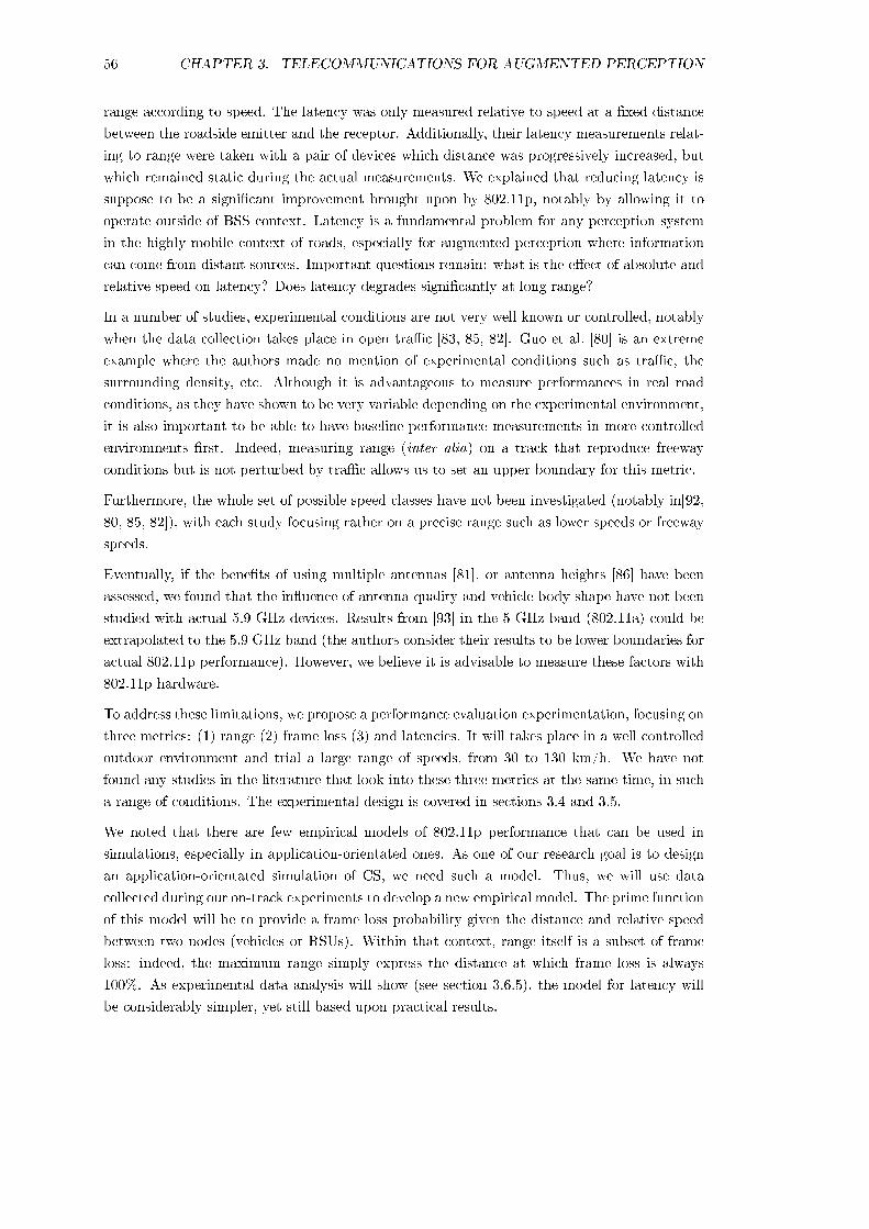
56 CHAPTER 3. TELECOMMUNICATIONS FOR AUGMENTED PERCEPTION

range according to speed. The latency was only measured relative to speed at a xed distance

between the roadside emitter and the receptor. Additionally, their latency measurements relat-

ing to range were taken with a pair of devices which distance was progressively increased, but

which remained static during the actual measurements. We explained that reducing latency is

suppose to be a signicant improvement brought upon by 802.11p, notably by allowing it to

operate outside of BSS context. Latency is a fundamental problem for any perception system

in the highly mobile context of roads, especially for augmented perception where information

can come from distant sources. Important questions remain: what is the eect of absolute and

relative speed on latency? Does latency degrades signicantly at long range?

In a number of studies, experimental conditions are not very well known or controlled, notably

when the data collection takes place in open trac [83, 85, 82]. Guo et al. [80] is an extreme

example where the authors made no mention of experimental conditions such as trac, the

surrounding density, etc. Although it is advantageous to measure performances in real road

conditions, as they have shown to be very variable depending on the experimental environment,

it is also important to be able to have baseline performance measurements in more controlled

environments rst. Indeed, measuring range (inter alia) on a track that reproduce freeway

conditions but is not perturbed by trac allows us to set an upper boundary for this metric.

Furthermore, the whole set of possible speed classes have not been investigated (notably in[92,

80, 85, 82]), with each study focusing rather on a precise range such as lower speeds or freeway

speeds.

Eventually, if the benets of using multiple antennas [81], or antenna heights [86] have been

assessed, we found that the inuence of antenna quality and vehicle body shape have not been

studied with actual 5.9 GHz devices. Results from [93] in the 5 GHz band (802.11a) could be

extrapolated to the 5.9 GHz band (the authors consider their results to be lower boundaries for

actual 802.11p performance). However, we believe it is advisable to measure these factors with

802.11p hardware.

To address these limitations, we propose a performance evaluation experimentation, focusing on

three metrics: (1) range (2) frame loss (3) and latencies. It will takes place in a well controlled

outdoor environment and trial a large range of speeds, from 30 to 130 km/h. We have not

found any studies in the literature that look into these three metrics at the same time, in such

a range of conditions. The experimental design is covered in sections 3.4 and 3.5.

We noted that there are few empirical models of 802.11p performance that can be used in

simulations, especially in application-orientated ones. As one of our research goal is to design

an application-orientated simulation of CS, we need such a model. Thus, we will use data

collected during our on-track experiments to develop a new empirical model. The prime function

of this model will be to provide a frame loss probability given the distance and relative speed

between two nodes (vehicles or RSUs). Within that context, range itself is a subset of frame

loss: indeed, the maximum range simply express the distance at which frame loss is always

100%. As experimental data analysis will show (see section 3.6.5), the model for latency will

be considerably simpler, yet still based upon practical results.

3.3. EXPERIMENTAL REQUIREMENTS 57

3.3 Experimental requirements

In the previous section, we argued that a new set of experimental evaluation of 802.11p was

necessary to address several limitations within the state-of-the-art. In this section, we will

discuss the experimental requirements for such an evaluation. They cover a number of dierent

themes, and will be presented in a synthetic format to ease reading and referencing.

Requirements concerning the environment

The environment in which data collection will take place must:

Possess road-like surroundings which exclude for example (former) airport runways.

Be a closed (private) environment to avoid trac disturbance.

Allow the use of a variety of node density, from low (e.g. 2 vehicles) to high (e.g. 5

vehicles and 5 RSUs) densities.

Requirements concerning the 802.11p devices

The 802.11p devices which will be used for the data collection must:

Be inexpensive, using mostly pre-existing hardware, so that they are not too far away

from future commercial applications.

Use a common hardware and software architecture for all experimental scenarios.

Use an open-source 802.11p driver.

Allow complete control over the software suites, so that all parameters can be known and

edited if required by the experimental protocol.

Be able to work equally in IPv4 and IPv6 (allowing inter-operability with future IPv6

systems).

Requirements concerning the experimental protocol

The experimental protocol used for the data collection must:

Cover speeds that represent the whole variety of roads, from small local trac roads to

freeways.

Ensure that measurements at each speed are repeated enough for the results to be stat-

istically signicant.

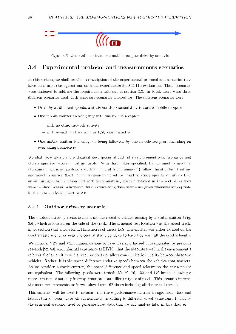
58 CHAPTER 3. TELECOMMUNICATIONS FOR AUGMENTED PERCEPTION

Figure 3.6: One static emitter, one mobile receptor drive-by scenario

3.4 Experimental protocol and measurements scenarios

In this section, we shall provide a description of the experimental protocol and scenarios that

have been used throughout our on-track experiments for 802.11p evaluation. These scenarios

were designed to address the requirements laid out in section 3.3. In total, there were three

dierent scenarios used, with some sub-scenarios allowed for. The dierent scenarios were:

Drive-by at dierent speeds, a static emitter transmitting toward a mobile receptor

One mobile emitter crossing way with one mobile receptor

with no other network activity

with several emitter-receptor RSU couples active

One mobile emitter following, or being followed, by one mobile receptor, including an

overtaking manoeuvre

We shall now give a more detailed description of each of the aforementioned scenarios and

their respective experimental protocols. Note that unless specied, the parameters used for

the communications (payload size, frequency of frame emission) follow the standard that are

addressed in section 3.5.3. Some measurement setups, used to study specic questions that

arose during data collection and with early analysis, are not detailed in this section as they

were ad-hoc scenarios however, details concerning these setups are given whenever appropriate

in the data analysis in section 3.6.

3.4.1 Outdoor drive-by scenario

The outdoor drive-by scenario has a mobile receptor vehicle passing by a static emitter (Fig.

3.6), which is located on the side of the track. The principal test location was the speed track,

in its section that allows for 1.4 kilometres of direct LoS. The emitter was either located on the

track's eastern end, or near the central slight bend, so to have LoS with all the track's length.

We consider V2V and V2I communications to be equivalent. Indeed, it is suggested by previous

research [92, 83], and informal experience at LIVIC, that the absolute speed in the environment's

referential of an emitter and a receptor does not aect communication quality between these two

vehicles. Rather, it is the speed dierence (relative speed) between the vehicles that matters.

As we consider a static emitter, the speed dierence and speed relative to the environment

are equivalent. The following speeds were tested: 30, 50, 70, 130 and 170 km/h, allowing a

representation of not only freeway situations, but dierent types of roads. This scenario features

the most measurements, as it was played out 162 times including all the tested speeds.

This scenario will be used to measure the three performance metrics (range, frame loss and

latency) in a clean network environment, according to dierent speed variations. It will be

the principal scenario, used to generate most data that we will analyse later in this chapter.

3.4. EXPERIMENTAL PROTOCOL AND MEASUREMENTS SCENARIOS 59

Figure 3.7: One emitter, one receptor crossing scenario

Figure 3.8: Three emitters (1 OBU + 2 RSU), two receptors (1 OBU + 1 RSU) crossing scenario

3.4.2 Outdoor crossing scenarios

The outdoor crossing scenario has a receptor vehicle passing by an emitter vehicle, both mobile.

The principal test location was the speed track. Two sub-scenarios are considered.

A rst, clean sub-scenario where there is only one emitter and one receptor (Fig. 3.7). Each

vehicle started at one end of the track, outside of direct view from the other and drove the

whole track at constant speed before turning around in the roundabout end. The location

of the crossing event moved depending on each vehicle's speed (it usually took place in the

western-most third of the track's eastern section). For this sub-scenario, the following speeds

were tested: 30, 70, and 130 km/h, which in terms of relative speeds between the two vehicle

gives: 60, 140 and 260 Km/h.

A second, noisy sub-scenario where there is not only the two vehicles but also three roadside

units, of which two are emitting (unicasting) a constant data stream (on the same channel)

toward the third one (Fig. 3.8). Although the java sender/receiver in the receptor vehicle does

not record frames sent by the RSUs, they are available in the Wireshark (a well-known network

performance monitoring tool) log, as well as in the java sender/receiver in the receptor RSU.

The RSUs are arranged so that the receptor one is surrounded by the two others, about 50

metres on each side. Each vehicle started at one end of the track, outside of direct view from

the other and drove towards the noisy area formed by the RSUs; drivers were instructed to

try at their best to cross in the middle of the noisy area, while maintaining constant speed as

they approached and receded from it. The vehicles drove only at 50 km/h in this sub-scenario.

For this sub-scenario, the communication parameters varied. The following parameters were

used at the emitter vehicle (the noise communication between the RSU remained constant, with

500 bytes payloads sent at 20 Hz):

1. 50 bytes payload sent each 25 milliseconds (40 Hz)

2. 500 bytes payload sent each 50 milliseconds (20 Hz)

3. 1 kilobytes payload sent each 500 milliseconds (2 Hz)

The crossing scenarios will be used, rstly, to conrm that V2V and V2I are equivalent; then

most importantly, it will be used to quantify the inuence of other active emitters upon the

latency of frame exchanged between the two vehicles.

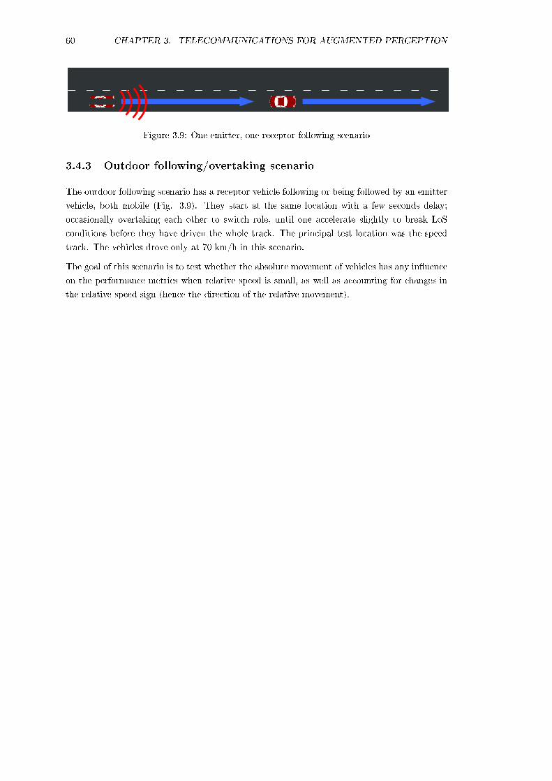
60 CHAPTER 3. TELECOMMUNICATIONS FOR AUGMENTED PERCEPTION

Figure 3.9: One emitter, one receptor following scenario

3.4.3 Outdoor following/overtaking scenario

The outdoor following scenario has a receptor vehicle following or being followed by an emitter

vehicle, both mobile (Fig. 3.9). They start at the same location with a few seconds delay;

occasionally overtaking each other to switch role, until one accelerate slightly to break LoS

conditions before they have driven the whole track. The principal test location was the speed

track. The vehicles drove only at 70 km/h in this scenario.

The goal of this scenario is to test whether the absolute movement of vehicles has any inuence

on the performance metrics when relative speed is small, as well as accounting for changes in

the relative speed sign (hence the direction of the relative movement).

3.5. EXPERIMENTAL SET-UP 61

3.5 802.11p devices implementation and measurements set-

up

In this section, we shall provide a detailed description of the hardware and software architecture

that have been used throughout our on-track experiments related to 802.11p evaluation, as well

as the supporting non-IT and non-ionic hardware (typically test vehicles) and infrastructure.

For most of the measurements, we have restrained ourselves to a limited number of tools, which

streamlined the experimental developments and allowed us to compare data more easily.

3.5.1 IVC devices

3.5.1.1 Rationale for using existing hardware

802.11p is still a relatively new technology, as such the number of standardised o-the-shelf

IVC devices (IVCD) remain limited. This is likely to remain true as long as all regulatory

authorities do not nalise spectrum bands allocation. Nevertheless, a few providers do oer

hardware suites, such as Denso (Germany) and Cohda Wireless (Australia). There are also

numerous prototype equipment available to researchers, providing they have taken part of CS-

related projects. The LIVIC has been involved in two CS projects: CVIS7 and COOPERS8.

As part of these projects, the best reasonably-priced 802.11p technology available had been

selected, and similar devices are still in use in many ongoing research programs. Thus, we chose

to re-use hardware from these previous studies for the purpose of our research.

As well as limiting expenses, re-using hardware from previous projects also allowed us to come

up with using a system running completely on open-source software, or on locally-developed one.

Indeed, one of the principal limitations of o-the-shelf or software from previous projects is that

it often includes, if not completely made of, proprietary code. An example of these functional,

yet limited, software is the original 802.11p drivers developed as part of the CVIS project. After

the CVIS project ended in 2010, it became increasingly dicult to access documentation and

support for these drivers. Licensing questions also remained unresolved. Furthermore, assessing

802.11p performances requires an important level of control over the IVCD; many parameters

need, or might need to be adjusted. This level of control is best attainable with open-source

and LIVIC-developed software. Thus, focusing on an open-source implementation was our best

chance in gaining access to reliable devices.

3.5.1.2 IVCD system's characteristics

Our IVCD is based on an ALIX 3D3 system board. It was initially designed for wireless

routing and network security applications, but can be also used for in-vehicle application as

well. It has already been used in several CS projects, where a 500 MHz single core processor

is enough to sustain IVC networking and some safety-related applications. To access wireless

LAN (WiFi), and 802.11p in particular, the system board is tted with an Atheros 5413 WiFi

chipset. Already used for CVIS hardware, 5413 chipsets are primarily 802.11abg, but have been

modied by the manufacturer to access 802.11p channels, providing the appropriate drivers are

7www.cvisproject.org8www.coopers-ip.eu

62 CHAPTER 3. TELECOMMUNICATIONS FOR AUGMENTED PERCEPTION

used. The only other notable hardware on the ALIX 3D3 boards are their 8 gigabytes solid-state

drive memories.

Regarding the board's functions within our architecture, there was no need for a complex

operating system. Thus, we chose to use a command line-only version of Linux Ubuntu (also

note that the device's memory can barely support a graphical operating system). The system

can use IPv4 or IPv6, depending on the requirements of the experiment (most of the time, IPv4

was used).

As we mentioned in 3.5.1.1, we focus on using open-source resources for the IVCD. Unfortu-

nately, open-source resources for 802.11p are quite limited, due to the amendment's young age,

as well as a signicant focus on simulation studies instead of actual implementations. The prin-

cipal open-source WiFi driver for Atheros chipsets (802.11abg) on Linux is the ath5K driver9, a

part of the MadWi drivers set. A patch developed for the Dutch Grand Cooperative Driving

Challenge (GCDC) 10 in 2010 allows this driver to operate within the 802.11p framework. The

drivers used in CVIS were also based on ath5k, and the GCDC patch actually emulates CVIS

drivers functionalities (it is also distributed with a CALM manager).

As part of our IVCD, only the patched ath5k is used. For the best performance and stability,

the patch limited the IVCD to the 2.6.31 version of Linux's kernel, with Ubuntu 9.10 (Karmic

Koala).

Implementing the patched driver on our IVDC was a signicant Challenge due to limited doc-

umentation available and involved many incremental trials. Eventually, thanks to the help of

researchers11 involved in the development of the patch, we managed to obtain a functional

802.11p-enabled system. We wrote a document enhancing the original documentation, which

was then distributed to the patch's developers; a copy of this document is available in Appendix

A.

Eventually, we installed on the IVDC the CarGeo6 framework. CarGeo6 is an open-source

system allowing the use of geographical networking and routing in IPv6, developed at the

INRIA as part of the GeoNet European project12. Georouting presents a strong potential for

CS applications, and especially augmented perception. It was initially used for the emergency

braking application that we implemented as discussed in Chapter 2. Even though we did not

use it for the rest of our study, including the 802.11p performance evaluation, we also installed

it on our IVCD with future research in mind.

As of mid-2012, 13 IVCD have been created, via cloning of the solid-state drives. Since all the

devices are essentially identical, only a few parameter changes were required for a newly copied

device to be connected to the network.

Our inexpensive, open-source, completely controllable and easy-to-replicate 802.11p-enabled

IVCD is a signicant engineering outcome of this thesis. Previous IVCD used at LIVIC have

been superseded by our version, and we expect future research on IVC and CS to continue using

this setting. They have already been used for several demonstrations to high-level executives

within the French government, including the Minister of Higher Education and Research.

9linuxwireless.org/en/users/Drivers/ath5k10www.gcdc.net/mainmenu/Home/technology/Communication_Stack11We thank the following people for their help in this matter: Sagar Behere, from the KTH Royal Institute

of Technology, Sweden; Anh Tuan Giang, from the École Supérieure d'Électricité, France; Jan de Jongh, fromTNO, the Netherlands; Kristoer Lidström, from the Viktoria Institute, Sweden; and Holger Rapp, from theKarlsruhe Institute of Technology, Germany.

12www.geonet-project.eu

3.5. EXPERIMENTAL SET-UP 63

802.11pantenna

GPS

Switch

NTP server

Ethernet

IVC device

Coaxialcable

Ethernet

Host PC

Ethernet

GPS RTK

Serial portconnection

Figure 3.10: Hardware architecture used for the measurements

3.5.2 Hardware architecture

Despite the diversity of the scenarios, our measurements could be performed with similar hard-

ware architecture, as they shared the same requirements:

Using our IVCD for 802.11p networking and applications hosting

Availability of precise localisation sensors

Time synchronisation

To full these requirements, our experimental architecture features an IVCD, a host computer,

a GPS device (RTK or classical) and a NTP time server, as seen in Fig. 3.10. Connection

to the vehicle's CAN bus and/or to an inertial navigation unit is possible, if the host vehicle is

tted with such system(s), although it was not a requirement in most cases. The architecture

is duplicated in each vehicle and roadside units (RSU).

IVC device

The IVCD is connected to a roof-mounted omnidirectional stick antenna13, with a 8 dBi gain

in the horizontal plane. The chipset's transmission power is lowered to 20 dBm. The Eective

Isotropically Radiated Power (EIRP) can be used to approximate the actual power output at

the antennas. It can be computed from equation 3.1:

EIRP = Ptx +G− Lc (3.1)

where Ptx is the transmission power at the emitter (dBm); G is the antenna gain, relative to

a (theoretical) isotropic reference antenna, in dBi; and Lc represents cable and connectors loss

(in dB). In our architecture Lc is approximated from manufacturers' data to 2.5 dB, accounting

for one pigtail connector, the eciency of the antenna, and about 2 metres of coaxial cable.

13Antenna's reference: Doradus 50-1360, 5.0 to 5.9 GHz

64 CHAPTER 3. TELECOMMUNICATIONS FOR AUGMENTED PERCEPTION

EIRP (dBm) EIRP (milliwatts)

40 1000036 400030 100025 32020 10015 3210 105 3.21 1.30 1-1 0.79-5 0.32-10 0.1-20 0.01-40 0.0001-80 0.00000001

Table 3.2: EIRP conversion chart, dBm to mW

Thus, we have EIRP = 20 − 2.5 + 8 = 25.5 dBm, or 355 mW (refer to Table 3.2 for dBm to

mW conversion). This value was used in all measurements drives, unless stated otherwise.

One could note that with EIRP = 25.5 dBm, we were largely under the regulatory limits im-

posed by telecommunication regulatory agencies, as described in section 3.2.4.2. Indeed, in the

European Union, the maximum EIRP in the 802.11p 5.9 GHz band is 33 dBm (2 watts). It was

our understanding that it would be unlikely that in the future 802.11p-based CS applications

would use the maximum allowed transmission power at all times, especially when the number

of connected actors would have signicantly grown. Also, American regulations specify a max-

imum EIRP for some channels of only 23 dBm, with short range services in mind. For these

reasons, it is more interesting to evaluate 802.11p performance at a non-extreme, intermediate

power output.

In terms of practical implementation, we had access to a limited number of antennas. We

could choose between small 1 dBi antennas of several shapes, and larger 8 dBi stick antennas.

Informal measurements were used to determine which were the most appropriate for our future

experiments, keeping in mind that we had to be able to (1) remain under regulatory limits at

all times and (2) allow signal's natural extinction within line of sight and more importantly,

within the 802.11p's theoretical range of 1 kilometre. Eventually, we settled on using the large,

8 dBi-gain antennas with a reduced power output at the chipset.

It is necessary to add that the test tracks are located in the vicinity of telecommunication

equipments operated by the French military police, thus further stressing the need to stick to

regulatory transmission power limits.

For all experiments, the devices are set to operate on the control channel adopted in the USA

for ITS, i.e. 5.890 GHz.

Host computer and GPS

The host computer's prime function is to record the vehicles' location, but it can also be used

to host applications that require too much processing power to be installed on the IVCD.

3.5. EXPERIMENTAL SET-UP 65

Table 3.3: Summary of 802.11p and frames parameters

Parameter Value

Frequency 5.890 GHzTX power (at chipset) 20 dBmAntenna type, gain Omnidirectional, 8 dBi

EIRP ~25.5 dBm (355 mW)Frame size > 84 bytes

Frame frequency 20 HzData rate auto (max 36 Mb/s)

Additionally, any application requiring a graphical interface have to be run by it, as the IVCD

uses a command-line OS.

In most of our measurements, the host PC was connected to a RTK GPS device updating at

two to ve Hertz. Actually, any type of GPS device could be used, as the software tasked with

recording the host vehicle's localisation did not dierentiate between specic versions of GPS

(it is able to handle higher frequency inputs). Our prime GPS device was a RTK GPS from

Thales, with its base station installed in the middle of Satory's tracks.

GPS performance have been sucient during most measurements, with lane-level accuracy

(typically within 1 metre). Although we did not require a centimetric accuracy, we have noted

worrying uctuations in accuracy at some times, with positioning errors of several dozen metres

or more. Since the distance between the emitter and the receptor was computed using linear

interpolation and the jumps in GPS positions were relatively limited in duration, these errors

did not aect the accuracy of our telecommunication measurements. However, their impact

could be much stronger on the augmented map, and the presence of such errors in a relatively

simple conguration such as Satory's tracks reinforces the case for using data fusion approaches

to improve the accuracy of localisation and perception of the environment.

NTP time server

Time synchronisation is critical for dierent functionalities - fusion of remote data, accurate

evaluation of latencies between dierent hosts, etc. Even if our devices' clocks were not of

the lowest quality, it is nevertheless necessary to ensure good synchronisation by correcting

clock drift at all times. Indeed, unsynchronised IVCD will drift by several seconds over a day

compared to an absolute time reference.

A straightforward way to do so is to use the Network Time Protocol (NTP). We installed

one Brandywine Network Time Adapter14 (BNTA) in each host vehicle or RSU, to distribute

accurate timing information from GPS through a NTP architecture. Within the NTP parlance,

the BNTA is a stratum 1 time server, as it is directly referenced to GPS satellite-based clocks

(stratum 0). As such, the IVCD and host computer are clients of stratum 2. The BNTA is set

in broadcast mode, sending timing information to its clients four times a second.

This system's performances have been excellent, most of the time. The oset between the GPS

reference time and our devices' clocks was smaller than one millisecond. An example of the

oset measured during data collection is shown in Fig. 3.11; the oset presented was recorded

on the receptor vehicle on 5 October 2011, the grey bars represent the error in the measurement,

as computed by the NTP algorithm. This error depends principally on (1) the number of visible

14http://www.brandywinecomm.com/images/NTA-100GM_datasheet.pdf

66 CHAPTER 3. TELECOMMUNICATIONS FOR AUGMENTED PERCEPTION

-0.01

-0.005

0

0.005

0.01

0.015

15:36 15:50 16:04 16:19 16:33 16:48 17:02 17:16 17:31 17:45

Time (date of recording: 05-Oct-2011)

Off

set

(sec

on

d)

Figure 3.11: Variation of oset between the GPS reference time and the IVCD's clock over a 2hour period

GPS satellites and (2) the quality of the in-vehicle wired network linking the BNTA and its

client(s).

3.5.3 Software architecture

Similarly with the hardware architecture, a single software architecture was able to answer

most of our requirements for data collection in the dierent experimental scenarios. However,

a diversity of software could be used to achieve this. The overall software architecture is shown

in Fig. 3.12; it features dierent software solutions that could be used for the same role. As

with the hardware, the architecture is duplicated in all vehicles and RSU, with only the need

to update some conguration les to have the architecture behave either as receptor or emitter.

All devices operate on Linux OS.

Network performance application

The software architecture's central element is the software used to generate and record frames,

which are exchanged on the 802.11p network. We had several methods to apply this, two of

which are entirely contained on the IVCD.

The rst method was to use the iperf tool on the IVCD. Iperf is a widely used network tool that

can be used to measure various network performances. It is primarily used for wired networks,

but can be used with wireless networks without diculties. It generates TCP or UDP data

streams between a server and a client, and can be set for half or full duplex connectivity. Bitrate

and frame loss are immediately available in iperf 's logs however, latency cannot be measured

with it.

3.5. EXPERIMENTAL SET-UP 67

R T M a p sN T P c l i e n t

E D A D r i v e r E t h e r n e t

I p e r f

J a v a a p p l i c a t i o n

D r iv e r 8 0 2 . 1 1 p ( a t h 5 k )

N T P c l i e n t

G P S R T K N T P S e r v e r

H o s t P C

I V C d e v i c e

W i r e le s sm e d iu m

Figure 3.12: Software architecture used for the measurements

To compensate for iperf 's limitations, we developed a second method entirely hosted on the

IVCD. It is a Java application that can be set as sender or receiver (henceforth the Java

sender/receiver), and is controlled via shell les (example on Fig. 3.13). It sends a UDP frame

through a Java datagram socket (equivalent to any other raw socket) to the IP address of the

target vehicle, at a frequency set by the user. The default frequency is 20 Hz (deterministic

timer). Data rate is automatically determined by the chipset and uctuates from 6 to 54 Mb/s,

depending on the signal/noise ratio.

A typical payload size is 20 bytes however, it can vary by up to 10 bytes because of the

increased length of the frame number eld (see Table 3.4). The actual frame at the MAC

level also includes 8 bytes of UDP header, 20 bytes of IP header, 8 bytes for LLC, and 28

additional bytes of overheads including the 802.11 MAC preamble and header, as well as the

CRC sequence. Thus, with a payload if 20 bytes, a MAC frame reaches 84 bytes. As our focus

was primarily on collision alert dissemination (e.g. EEBL), we chose to use a frame size in line

with EEBL's requirements. In [32], the recommended payload for EEBL frames is 36 bytes,

and includes detailed information on the emitter's behaviour. Some data elds listed in the

cited report, such as the vehicle's size and the GPS antenna's oset can be removed without

aecting the application's usefulness. We believe 20 to 30 bytes is a good compromise for an

EEBL frame that can include a vehicle's ID, location and timing information. The frame's

structure is shown in Table 3.4.

The application automatically computes the latency based on the frame's emission time, as

recorded in its payload. A log le is automatically generated containing the frame's information:

computed latency, payload size, received power (signal strength indicator) and reception time.

Frame loss and bitrate can then be processed from this log le (a log extract is shown in Fig.

3.13c). This application was the principal one we used during data collection.

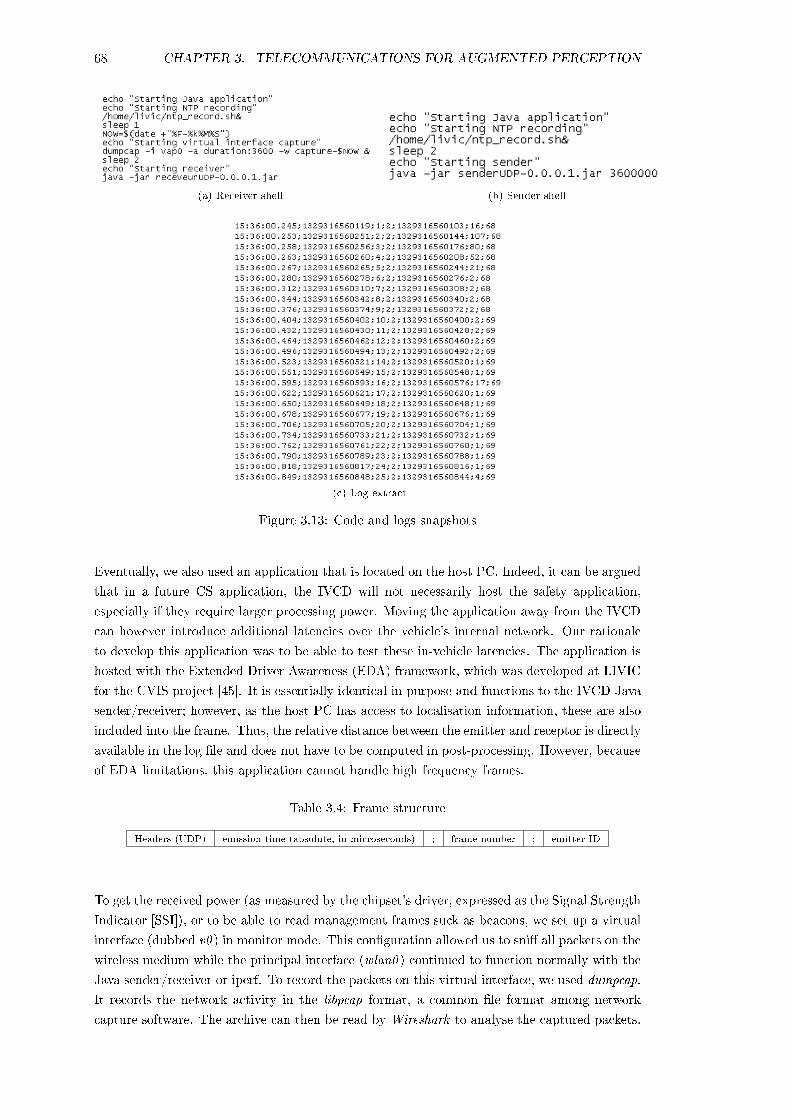
68 CHAPTER 3. TELECOMMUNICATIONS FOR AUGMENTED PERCEPTION

(a) Receiver shell (b) Sender shell

(c) Log extract

Figure 3.13: Code and logs snapshots

Eventually, we also used an application that is located on the host PC. Indeed, it can be argued

that in a future CS application, the IVCD will not necessarily host the safety application,

especially if they require larger processing power. Moving the application away from the IVCD

can however introduce additional latencies over the vehicle's internal network. Our rationale

to develop this application was to be able to test these in-vehicle latencies. The application is

hosted with the Extended Driver Awareness (EDA) framework, which was developed at LIVIC

for the CVIS project [45]. It is essentially identical in purpose and functions to the IVCD Java

sender/receiver; however, as the host PC has access to localisation information, these are also

included into the frame. Thus, the relative distance between the emitter and receptor is directly

available in the log le and does not have to be computed in post-processing. However, because

of EDA limitations, this application cannot handle high frequency frames.

Table 3.4: Frame structure

Headers (UDP) emission time (absolute, in microseconds) ; frame number ; emitter ID

To get the received power (as measured by the chipset's driver, expressed as the Signal Strength

Indicator [SSI]), or to be able to read management frames suck as beacons, we set up a virtual

interface (dubbed v0 ) in monitor mode. This conguration allowed us to sni all packets on the

wireless medium while the principal interface (wlan0 ) continued to function normally with the

Java sender/receiver or iperf. To record the packets on this virtual interface, we used dumpcap.

It records the network activity in the libpcap format, a common le format among network

capture software. The archive can then be read by Wireshark to analyse the captured packets.

3.5. EXPERIMENTAL SET-UP 69

root@cargeo6-router2:~# ping 192.168.99.1 -I wlan0PING 192.168.99.1 (192.168.99.1) from 192.168.99.2 wlan0: 56(84) bytes of data.64 bytes from 192.168.99.1: icmp_seq=1 ttl=64 time=4.460 ms64 bytes from 192.168.99.1: icmp_seq=2 ttl=64 time=0.416 ms64 bytes from 192.168.99.1: icmp_seq=3 ttl=64 time=0.428 ms64 bytes from 192.168.99.1: icmp_seq=4 ttl=64 time=0.414 ms64 bytes from 192.168.99.1: icmp_seq=5 ttl=64 time=0.408 ms64 bytes from 192.168.99.1: icmp_seq=6 ttl=64 time=0.392 ms64 bytes from 192.168.99.1: icmp_seq=7 ttl=64 time=0.410 ms64 bytes from 192.168.99.1: icmp_seq=8 ttl=64 time=0.415 ms64 bytes from 192.168.99.1: icmp_seq=9 ttl=64 time=0.411 ms64 bytes from 192.168.99.1: icmp_seq=10 ttl=64 time=0.409 ms

(a) IPv4

root@cargeo6-router2:~# ping6 2011:192:168:ca01:147:e0ff:fe55:991 -I wlan0PING 2011:192:168:ca01:147:e0ff:fe55:991(2011:192:168:ca01:147:e0ff:fe55:991)from 2011:192:168:ca01:147:e0ff:fe55:992 wlan0: 56 data bytes64 bytes from 2011:192:168:ca01:147:e0ff:fe55:991: icmp_seq=1 ttl=64 time=4.310 ms64 bytes from 2011:192:168:ca01:147:e0ff:fe55:991: icmp_seq=2 ttl=64 time=0.831 ms64 bytes from 2011:192:168:ca01:147:e0ff:fe55:991: icmp_seq=3 ttl=64 time=0.785 ms64 bytes from 2011:192:168:ca01:147:e0ff:fe55:991: icmp_seq=4 ttl=64 time=0.822 ms64 bytes from 2011:192:168:ca01:147:e0ff:fe55:991: icmp_seq=5 ttl=64 time=0.818 ms64 bytes from 2011:192:168:ca01:147:e0ff:fe55:991: icmp_seq=6 ttl=64 time=0.750 ms64 bytes from 2011:192:168:ca01:147:e0ff:fe55:991: icmp_seq=7 ttl=64 time=0.611 ms64 bytes from 2011:192:168:ca01:147:e0ff:fe55:991: icmp_seq=8 ttl=64 time=0.508 ms64 bytes from 2011:192:168:ca01:147:e0ff:fe55:991: icmp_seq=9 ttl=64 time=0.457 ms64 bytes from 2011:192:168:ca01:147:e0ff:fe55:991: icmp_seq=10 ttl=64 time=0.467 ms

(b) IPv6

Figure 3.14: Latencies for ICMP echo requests over a 802.11p ad-hoc network, at short range,in IPv4 and IPv6

802.11p specic

As we mentioned in section 3.2.4, one important change that was introduced by the 802.11p

amendment is the ability for a 802.11p device to operate outside of the classical BSS context by

using the dot11OCBEnabled ag. This functionality is designed to be used with high priority

emergency-related frames, as it shrinks transmission delays as much as possible within the

802.11 architecture.

We chose to maintain the dot11OCBEnabled ag to false, meaning that the normal BSS context

is in use. Indeed, not all frames exchanged within a VANET during normal, day-to-day use will

require a high priority. It can be argued that in order to maintain the advantage of priority

management, the number of high priority frames must be limited. Thus, it is unlikely that

augmented perception-related messages will be high priority (though, they will be of higher

priority than frames which payload have less stringent latency requirements). Furthermore,

frames that contain critical information about a vehicle's location and behaviour need to be

secured, which would not be possible outside of a BSS context. Setting dot11OCBEnabled to

true for an collision alert dissemination makes more sense.

However, latencies measured within a BSS context for collision alert frames will provide an

upper boundary for latency outside of BSS context. Indeed, the OCB mechanism removes

authentication and other upper-layer dealings, but remain essentially identical at the MAC

level. If good latency performance is found within a BSS context, it will be possible to safely

conclude that the same performance would be achieved outside a BSS context.

Eventually, while focused on collision alert dissemination (as far as protocol is concerned), we

aim at assessing performance metrics of 802.11p in general, so given that frames outside of BSS

context would represent only a minority of the total frames exchanged, it is logical to remain

within a classic BSS context.

Other network functions

All network functionalities (physical, data link, network and transports layers) are managed

either with Linux's native protocols or by the patched ath5k WiFi driver (as detailed in 3.5.1).

Routing is handled with a manually-inputed routes table, or with CarGeo6. Note that iperf

and our applications are indierent to the exact version of the IP protocol used. Most of our

measurements used IPv4 for the sake of simplicity, but could have equally been made with

IPv6; the principal dierence with IPv6 would be a slightly increased latency; this is shown in

Fig. 3.14. CarGeo6 operates exclusively in IPv6.

70 CHAPTER 3. TELECOMMUNICATIONS FOR AUGMENTED PERCEPTION

Clock synchronisation

Both the IVCD and host computer use the NTP architecture to remain synchronised with an

external GPS reference clock, provided by the BNTA. An o-the-shelf Linux NTP client is used

on both machines.

Vehicle's localisation

The host PC is primarily tasked with recording its host vehicle's localisation. Data from a

GPS device (RTK or classical) is sent to one of the PC's serial port; this data stream is then

captured by the RTMaps software. RTMaps is marketed by Intempora15, based upon work

undertaken at Mines ParisTech a decade ago [94]. Its primary goal is to record and process a

large number of simultaneous data ows such as images, laserscanner scans, positioning data

(from GPS, odometer or INS), etc. It is also used to host algorithms for image processing or

data fusion for example, as we shall see further in this document.

3.5.4 Test vehicles at LIVIC

LIVIC is well equipped in terms of prototyping and experimental capabilities, with a eet of

six experimental vehicles, tted with various sensors, prototype hardware and software, ranging

from IVC to automated control. Three vehicles are used specically for IVC-related research:

two identical Renault Clio III 5-door estates and one Citroën C4 Grand Picasso 5-door MPV (see

Fig. 3.15). The vehicles were tted with powered equipment racks in the boot and several in-

cabin screens for HMI. A variety of sensors can be tted on them depending on the experimental

requirements; only one of the Clios had a permanent forward-facing radar.

3.5.5 Test tracks

The LIVIC is located immediately next to the Satory's test tracks (at the outskirts of Versailles).

The Satory's site is owned by the French Ministry of Defence, and was initially intended to test

armoured vehicles developed by Nexter (formerly GIAT Industries). It has since opened to

other private and public operators, including IFSTTAR, Citroën sports and Renault Trucks.

The site's most important features are its three test tracks, shown on gure 3.16a:

the speed track (la vitesse), a 2-lane 2 km straight line (orange on the map)

the road track (la routière), a 2-lane unidirectional 3.5 km loop (red)

the forest track (le Val d'Or), a 2-lane double loop set in small hillside wood (pink and

lila)

The speed track's surroundings are largely open, despite a few sections with over-reaching trees.

La routière track is modelled on French non-segregated trunk road (route nationale), and its

surroundings are also largely open, presenting a greater diversity than the speed track (it comes

close to several buildings).

15www.intempora.com

3.5. EXPERIMENTAL SET-UP 71

(a) Citroën C4 Grand Picasso (b) Renault Clio 3 (one of Tic & Tac)

Figure 3.15: Photographs of the test vehicles

(a) Map of the test tracks

(c) Looking westward (d) Looking eastward

(d) Photographs of the speed track (la vitesse), the track's bend appears in the distance, 1.2 km westward

Figure 3.16: Map and photographs of Satory's test tracks

72 CHAPTER 3. TELECOMMUNICATIONS FOR AUGMENTED PERCEPTION

3.6 Performance metrics analysis

3.6.1 Introduction

In this section, we shall analyse the data collected during our experiments. We will break down

the analysis by performance metrics, in the following order: (1) range, (2) latency, and (3)

frame loss. Each subsection will use data collected during dierent scenarios, as described in

section 3.4. This analysis will form the base upon which we will build our 802.11p model, as

described in section 3.7.

Data collection was spread out from September 2011 to February 2012, with a total of over

400 kilometres driven during experiments on the Satory test tracks. Meteorological conditions

were quite variable from day to day; most measurements took place on typical Parisian overcast

autumn or winter days, but we also gathered data during dry sunny conditions or light rain.

Unfortunately, we minimised a-priori the inuence of meteorological conditions, considering it

would not aect performance metrics, especially range, to a great amount. However, we will

see that meteorological conditions can create important performance variations.

Further in the performance analysis, two datasets will be described the 2011 and 2012 data-

sets. As their names suggest, these two dataset are only segregated by the time at which their

data were collected. The 2011 dataset was collected during 6 dierent days from September

to December 2011, and the 2012 dataset was collected during 4 days in January and February

2012. Each single day represents several hours of recording. The need to dierentiate into two

datasets arose from the fact that we did not take into account some important inuences on the

experimental data at the beginning, which were only discovered when the rst dataset (2011)

was analysed. Accordingly, more variables are controlled for in the second dataset; however,

the 2011 dataset contains a larger amount of data then the 2012 dataset (the repartition is

about 60-40% in favour of the 2011 dataset).

For the remainder of this chapter, closing will refer to items relevant to when the receptor

vehicle is moving toward the emitter; away will refer to items relevant to when the receptor

vehicle is moving away from the emitter.

3.6.2 Maximum range

3.6.2.1 General analysis

The range is the maximum distance at which a frame is successfully received by the receptor

vehicle from the emitter (when frame loss is almost 100%); thus what we call the range is

actually the transmission range. The physical carrier sensing range was not directly taken

into account, although it is possible to approximate it by looking at the underlying protocol

management frames. As described in section 3.5.2, the actual range value is estimated by linear

interpolation, in post-processing. The time of a frame reception is extracted and the two GPS

xes that comes immediately before and immediately after it are used as reference points. This

method is relatively accurate, thanks to the RTK GPS performance.

Fig. 3.17 is a box plot of all measured maximum ranges, classied according to speed (from

30 to 170 km/h) and direction of driving (left side, with the letter A, is the away set; right

3.6. PERFORMANCE METRICS ANALYSIS 73

30 A 50 A 70 A 130 A 170 A 30 C 50 C 70 C 130 C 170 C0

100

200

300

400

500

600

700

800

900

Speed (km/h) and driving direction (relative to the emitter)

Ran

ge

(met

res)

Away Closing

(a) Average and median maximum ranges and their dispersion, as computed on the 2011 dataset only

30 A 50 A 70 A 130 A 170 A 30 C 50 C 70 C 130 C 170 C0

250

500

750

1000

1250

1500

Speed (km/h) and driving direction (relative to the emitter)

Ran

ge

(met

res)

Away Closing

(b) Average and median maximum ranges and their dispersion, as computed on the whole measurements

Figure 3.17: Analysis of maximum transmission ranges obtained during our data collection

74 CHAPTER 3. TELECOMMUNICATIONS FOR AUGMENTED PERCEPTION

side, with the letter C, is the closing set). Fig. 3.17b is based on the whole data we collected,

while Fig. 3.17a shows only data from the 2011 dataset. The green x are the averages, while

the red lines shows the medians. The blue boxes and black whiskers shows the measurement's

dispersion: the boxes' edges represent the 25th and 75th percentiles, whiskers extend to the

most extreme data points not considered outliers. Outliers are shown as individual red crosses.

The median range (red lines) is not necessarily centred in the blue boxes, which shows that

maximum ranges are not evenly distributed and tend to concentrate around some values. For

example in 3.17a at 30 km/h away, 25% of the data is concentrated in the [680; 690] metres

interval. Data show a clear inverse relationship between relative speed and range.

The largest range for all measurements is 1,397 metres. Nonetheless, most of the measured

maximum ranges were largely under specications or ranges measured in other studies, espe-

cially in the 2011 dataset. As specied in Section 3.5.2, the transmission power was lowered to

remain in line with 802.11p specications. In [83], the transmission power was actually slightly

lower than ours (17 versus 20dBm, at the chipset), yet they achieved larger ranges. Given

that antennas gains were similar in both studies, [83]'s authors probably have used cables and

connectors with a lower attenuation than ours. However, the antennas' quality must probably

still have played a role to explain the dierence between our studies, as well shall see in 3.6.2.2.

Informal measurements with Tx power = 33 dBm (the maximum authorised transmission

power), suggested no diculty in achieving kilometric range systematically with larger powers.

However, given the antenna's gain, the EIRP was above the regulatory threshold in France

(and the EU), which disqualies such powers for future use. Furthermore, it is probable that

legally high-power transmissions will be restricted to a limited number of uses, in order to limit

physical medium saturation. This is the reason why high-powered (40+ dBm) transmissions

are only legal on 2 channels in the American spectrum allocation scheme, and strictly reserved

for governmental operations.

In Fig. 3.17a, one notes signicant dierences between the closing and away ranges at the same

speed (notably at 70 or 130 km/h), with the closing range being greater than away range, on

some occasions by up to 200 metres. This relates to ndings by Böhm et al. [83]; however, their

data are reverse compared to ours: away range is greater than closing range. The following

could be oered as an explanation: this eect can be explained by the mechanism of signal

validation in the Wi-Fi access points. This mechanism includes a hysteresis (or two thresholds)

to validate the signal. In fact, the receiver continues to accept the communication until the

signal power falls below a threshold S1. But to accept a new signal, it is necessary that is

power is larger than a threshold S2. In general S1 < S2, which means that the [away] range is

usually higher than the capture range [92]. However, this explanation does not apply to our

measurement, or Böhm et al., for several reasons. Both studies used ad-hoc mode instead of

access point. And in our study, closing range is systematically greater than away range in the

2011 dataset, while reverse measurements would be expected from [92]'s explanation.

Fig. 3.17b adds additional measurements taken at low speed (30 km/h), from the 2012 dataset.

These additional measurements are presented separately in Fig. 3.17a. As demonstrated on

the latter gure, there is no signicant dierence between closing and away ranges with those

measurements. The latter leads further credence to the fact that the power-level-based CCA and

CSMA/CA mechanisms used in 802.11p will not make any dierence to the vehicles' direction of

travel. Doppler eects likely only explain the range reduction with increased speeds, which was

veried for the whole data. We conclude that another eect must explain the original dataset's

behaviour; further analysis should be dedicated to investigate it in the following sub-sections.

3.6. PERFORMANCE METRICS ANALYSIS 75

Away Closing

1

1.05

1.1

1.15

1.2

1.25

1.3

1.35

1.4

1.45

Driving direction (speed is 30 km/h)

Ran

ge

(kilo

met

res)

Figure 3.18: Average and median maximum ranges and their dispersion, as computed on the2012 dataset only

3.6.2.2 Driving direction, car's body shape and antennas' imperfections

In order to investigate the dierence between closing and away range, we need to access MAC

layer frames directly. The only way to do so is to use the monitor mode. The monitor mode is a

standard 802.11 feature in which the chipset will send toward higher-level process all activities

that occur on the physical medium (at the frequency in use). All the hidden frames that are used

by the 802.11 standard, the so-called management frames, then become accessible. However,

when a wireless interface is set-up in monitor mode, it can only listen to the network, there

is no way to send frames. However, chipsets can support several interfaces at the same time.

Thus, by setting up a virtual interface working in monitor mode, management frames can be

recorded without disturbing the measurement process, while our application runs on the main

interface in ad-hoc mode.

We performed additional measurements in the exact same experimental conditions as previ-

ously, in order to conrm whether the user transmission on the IP stack had any eect on the

results. Our investigation suggests that there is no signicant dierence between the range for

management frames (beacons included) and for applications' frames in the speed track setting

(this is not clear cut in other settings, see 3.6.4). The direction of driving produces the same

inuence over the maximum range of beacons, which suggests that the dierence is due to an

actual physical eect.

Consequently, we have investigated the Signal Strength Indicator (SSI) for various speeds. The

SSI is measured by the Atheros chipset and included in the data passed to the upper layer; we

extracted it with Wireshark.

Fig. 3.19 shows the recorded SSI for a typical drive at 50 km/h, in both directions extracted

from the 2011 dataset. The gure shows that application frames (the smoothed lines) are

recorded as far as beacons (the crosses).

Furthermore, one can clearly see that two paths exist: the SSI is consistently lower when the

vehicle drives away, compared to when the vehicle drives toward the emitter. However, data

from the 2012 dataset, in otherwise exactly the same experimental conditions, do not show such

an hysteresis. Fig. 3.20 allows one to compare two measurements taken at the same speed, in

76 CHAPTER 3. TELECOMMUNICATIONS FOR AUGMENTED PERCEPTION

0 100 200 300 400 500 600 700−110

−100

−90

−80

−70

−60

−50

Range (metres)

SS

I (dB

m)

App. frames (away, smoothed)App. frames (closing, smoothed)Beacons (away)Beacons (closing)

Figure 3.19: SSI according to direction of driving, for beacons and application frames (singledrive pictured)

the same experimental conditions (location, vehicles, hardware, etc.) from the 2011 and 2012

datasets. The raw data have been smoothed using a Nadaraya-Watson kernel regression. The

dierence between the away and closing curves is much larger in the 2011 dataset than the

2012 dataset. The power dierence between the two dataset is explained by the dierence in

weather conditions and a better controlled experimental protocol in the 2012 dataset, so that

the received power is maximised in that dataset.

From these data, we assume that two factors could explain the hysteresis noted in the 2011

dataset, as well as the considerable dierence in received power (hence, range): (1) an imperfect

omnidirectionality of the antennas (in the horizontal plane), and (2) an inuence of the vehicle's

body. Indeed, during the 2011 dataset collection, the orientation of the antennas and vehicles

on the track (hence which side faced each other) was not controlled.

Antenna quality The antennas used during our experimentation are omnidirectional. Ac-

cording to the manufacturer's data, their gain varies on the horizontal plane by no more than

2 dB, with a good symmetry between the two sides of the antennas (the antenna's azimuthal

pattern is a slightly attened circle). We decided to verify whether this was really the case. At

rst, we focused on the receptor's antenna, as it was the one that would be aecting the most

received power during a normal experimental drive. Note that the same IVCD and antenna

pairs were always used for the same roles (emitter or receptor) throughout the measurements,

not only for the present experiment.

We measured the SSI for 8 orientations of the antenna, rotated 45 degrees each time from the

previous orientation. The initial orientation (angle 0) was chosen arbitrarily. The experimental

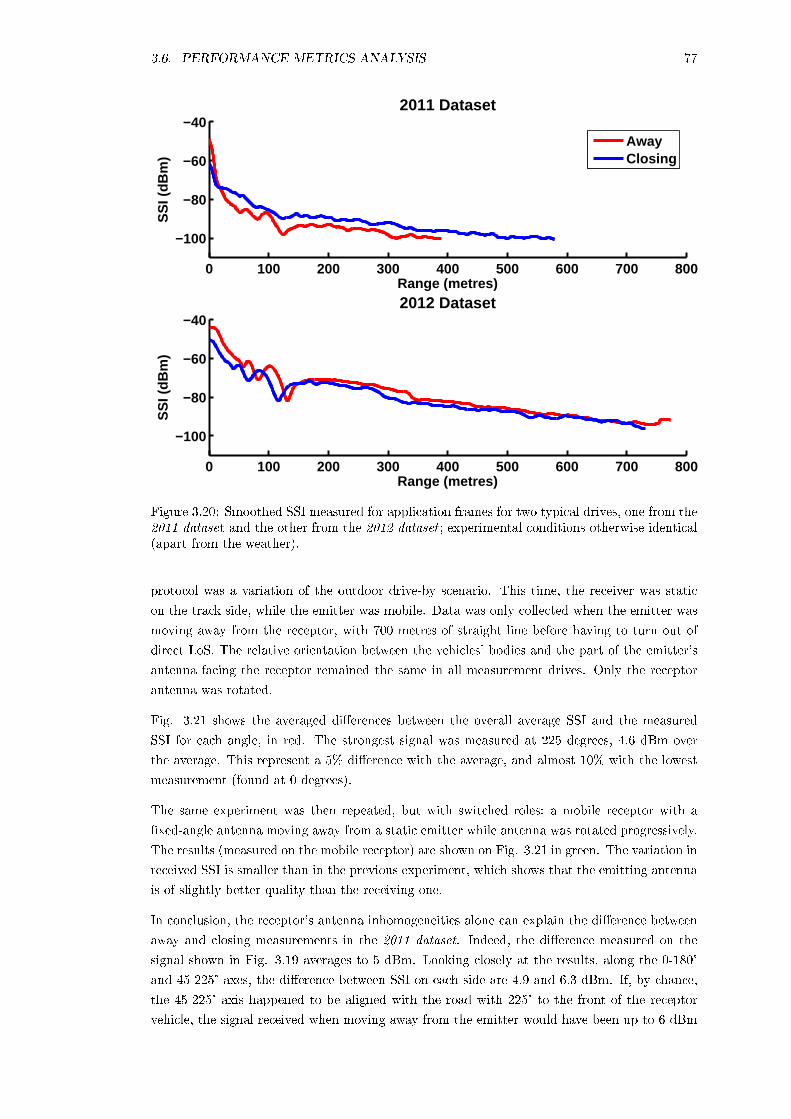
3.6. PERFORMANCE METRICS ANALYSIS 77

0 100 200 300 400 500 600 700 800

−100

−80

−60

−40

Range (metres)

SS

I (dB

m)

2011 Dataset

0 100 200 300 400 500 600 700 800

−100

−80

−60

−40

Range (metres)

SS

I (dB

m)

2012 Dataset

AwayClosing

Figure 3.20: Smoothed SSI measured for application frames for two typical drives, one from the2011 dataset and the other from the 2012 dataset ; experimental conditions otherwise identical(apart from the weather).

protocol was a variation of the outdoor drive-by scenario. This time, the receiver was static

on the track side, while the emitter was mobile. Data was only collected when the emitter was

moving away from the receptor, with 700 metres of straight line before having to turn out of

direct LoS. The relative orientation between the vehicles' bodies and the part of the emitter's

antenna facing the receptor remained the same in all measurement drives. Only the receptor

antenna was rotated.

Fig. 3.21 shows the averaged dierences between the overall average SSI and the measured

SSI for each angle, in red. The strongest signal was measured at 225 degrees, 4.6 dBm over

the average. This represent a 5% dierence with the average, and almost 10% with the lowest

measurement (found at 0 degrees).

The same experiment was then repeated, but with switched roles; a mobile receptor with a

xed-angle antenna moving away from a static emitter while antenna was rotated progressively.

The results (measured on the mobile receptor) are shown on Fig. 3.21 in green. The variation in

received SSI is smaller than in the previous experiment, which shows that the emitting antenna

is of slightly better quality than the receiving one.

In conclusion, the receptor's antenna inhomogeneities alone can explain the dierence between

away and closing measurements in the 2011 dataset. Indeed, the dierence measured on the

signal shown in Fig. 3.19 averages to 5 dBm. Looking closely at the results, along the 0-180°

and 45-225° axes, the dierence between SSI on each side are 4.9 and 6.3 dBm. If, by chance,

the 45-225° axis happened to be aligned with the road with 225° to the front of the receptor

vehicle, the signal received when moving away from the emitter would have been up to 6 dBm

78 CHAPTER 3. TELECOMMUNICATIONS FOR AUGMENTED PERCEPTION

-4

-2

0

2

4

60

45

90

135

180

225

270

315

Figure 3.21: Dierences with the average SSI (in dBm) for 8 angular sectors (in degrees) ofthe receiving antenna (in red) and of the emitting antenna (in green); measurements were notsimultaneous. The other antenna is always facing the measured sector.

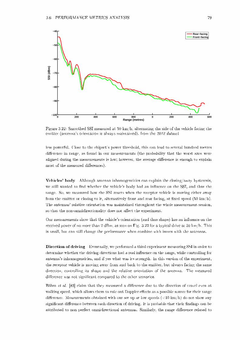
3.6. PERFORMANCE METRICS ANALYSIS 79

0 200 400 600 800 0 200 400 600−100

−90

−80

−70

−60

−50

−40

Range (metres)

SS

I (dB

m)

Rear−facingFront−facing

Figure 3.22: Smoothed SSI measured at 50 km/h, alternating the side of the vehicle facing theemitter (antenna's orientation is always maintained), from the 2012 dataset

less powerful. Close to the chipset's power threshold, this can lead to several hundred metres

dierence in range, as found in our measurements (the probability that the worst axes were

aligned during the measurements is low; however, the average dierence is enough to explain

most of the measured dierences).

Vehicles' body Although antenna inhomogeneities can explain the closing/away hysteresis,

we still wanted to nd whether the vehicle's body had an inuence on the SSI, and thus the

range. So, we measured how the SSI reacts when the receptor vehicle is moving either away

from the emitter or closing to it, alternatively front and rear-facing, at xed speed (50 km/h).

The antennas' relative orientation was maintained throughout the whole measurement session,

so that the non-omnidirectionality does not aect the experiment.

Our measurements show that the vehicle's orientation (and thus shape) has an inuence on the

received power of no more than 2 dBm, as seen on Fig. 3.22 for a typical drive at 50 km/h. This

is small, but can still change the performance when combine with issues with the antennas.

Direction of driving Eventually, we performed a third experiment measuring SSI in order to

determine whether the driving directions had a real inuence on the range, while controlling for

antenna's inhomogeneities, and if yes what was its strength. In this version of the experiment,

the receptor vehicle is moving away from and back to the emitter, but always facing the same

direction, controlling its shape and the relative orientation of the antenna. The measured

dierence was not signicant compared to the other scenarios.

Böhm et al. [83] claim that they measured a dierence due to the direction of travel even at

walking speed, which allows them to rule out Doppler eects as a possible source for their range

dierence. Measurements obtained with our set-up at low speeds (<10 km/h) do not show any

signicant dierence between each direction of driving. It is probable that their ndings can be

attributed to non perfect omnidirectional antennas. Similarly, the range dierence related to

80 CHAPTER 3. TELECOMMUNICATIONS FOR AUGMENTED PERCEPTION

the direction of driving that they found, at normal driving speeds, can probably be explained

by non-omnidirectionality.

3.6.3 Frame loss

Frame loss is dened as the percentage of frames that are missed during a certain measurement

interval, which we dene temporarily and according to range. It is straightforward to deduce

the actual bitrate from the nominal bitrate and the measured frame loss. The maximum range

is an important indicator, but does not say anything about the quality of transmissions within

this range. Typically, one could receive frames up to a thousand metres, yet have 90% frame loss

beginning as soon as 400 metres away from the emitter. Thus, it is also important to measure

the quality of transmission within the transmission range, typically via frame loss. Here, frame

loss is viewed from the logging application point of view. That means that any frame that is

not passed on to the IP layer is seen as lost. This include frames that are not received, or

only partially received, but also corrupted frames.

Fig. 3.23 presents the average and maximum (worst) frame loss measured over the whole

range, at 5-metre intervals. Both the 2011 and 2012 datasets are used (hence the continuing

classication along the direction of driving). Frame loss was initially computed each second,

before being re-projected on distance rather than time. One can note important uctuations

within the transmission range, at all speeds, of the maximum frame loss (red). However, one

should remember that the maximum (red) frame loss is dened by a single data point over the

whole datasets; that is why its uctuations are the most extreme. The average frame loss, in

green, shows less uctuations.

Another view of the average frame loss is given in Fig. 3.24 constructed on the 2011 dataset

only; this time the direction of the driving is not taken into account. This second graph

explains the incongruous shape of the 30 km/h average frame loss in Fig. 3.23, which results

from the interaction of the two datasets, creating patterns that are not representative of actual

measurements. This can be seen when the average and maximum frame loss starts to increase

after 400 metres (away) or after 700 metres (closing). In Fig. 3.24, the average frame loss

regardless of the driving direction increases sharply at 600 metres. The average does not reach

100% because data from other runs with much larger ranges are still accounted for at that

point, and these runs did not experience a rise in frame loss at these distances. The absence

of signicant dierence between the direction of movement in the 2012 dataset is visible here,

when looking at the maximum ranges (beyond 1,000 metres). The dip in average frame loss

around 1,300 metres in closing conditions is not an artefact; rather, we experienced a sudden

increase of the transmission quality at some point on the track, roughly corresponding to the

bend. This suggests some factors in the environment compounded to focus the emitter's signal,

decreasing the frame loss at the receptor for about 100 metres.

The uctuations of the average frame loss can also be explained by environmental features that

degrade the transmission's quality (scattering leading to multipath, interferences, degraded

LoS, etc.). A typical example is the destructive interferences that build up because of signal

reected from the ground (Two-Rays propagation model), which can be seen on most sub-

graphs at distances of 100-150 metres. Changing meteorological conditions aected the signal's

quality too.

Overall, the average frame loss shows that within range, the quality of transmission is reason-

able, but far from perfect.

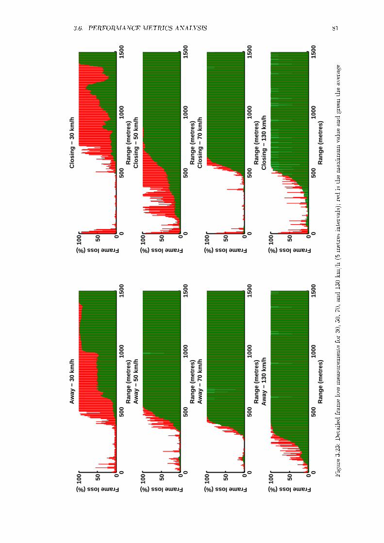
3.6. PERFORMANCE METRICS ANALYSIS 81

050

010

0015

00050100

Ran

ge (

met

res)

Frame loss (%)

Aw

ay −

30

km/h

050

010

0015

00050100

Ran

ge (

met

res)

Frame loss (%)

Clo

sing

− 3

0 km

/h

050

010

0015

00050100

Ran

ge (

met

res)

Frame loss (%)

Aw

ay −

50

km/h

050

010

0015

00050100

Ran

ge (

met

res)

Frame loss (%)

Clo

sing

− 5

0 km

/h

050

010

0015

00050100

Ran

ge (

met

res)

Frame loss (%)

Aw

ay −

70

km/h

050

010

0015

00050100

Ran

ge (

met

res)

Frame loss (%)

Clo

sing

− 7

0 km

/h

050

010

0015

00050100

Ran

ge (

met

res)

Frame loss (%)

Aw

ay −

130

km

/h

050

010

0015

00050100

Ran

ge (

met

res)

Frame loss (%)

Clo

sing

− 1

30 k

m/h

Figure

3.23:Detailed

frameloss

measurements

for30,50,70,and130km/h(5

metresintervals);redisthemaximum

valueandgreen

theaverage

82 CHAPTER 3. TELECOMMUNICATIONS FOR AUGMENTED PERCEPTION

0 200 400 600 800 10000

20

40

60

80

100

Range (metres)

Fra

me

loss

(%

)30 km/h

0 200 400 600 800 10000

20

40

60

80

100

Range (metres)

Fra

me

loss

(%

)

50 km/h

0 200 400 600 800 10000

20

40

60

80

100

Range (metres)

Fra

me

loss

(%

)

70 km/h

0 200 400 600 800 10000

20

40

60

80

100

Range (metres)

Fra

me

loss

(%

)

130 km/h

Figure 3.24: Average frame loss in the 2011 dataset, not accounting for direction of driving

3.6.4 Mapping transmission ranges and frame loss rates

After the principal outdoor drive-by scenario, where results have been detailed in previous

subsections, we performed additional measurements on la routière track, taking interest into

the perturbations introduced by objects in the environments. For this, we considered a I2V-like

scenario, where a roadside unit would service an area that featured medium density occulting

objects such as trees, buildings and mounds. All these would rise at least to the same height

as the RSU's antenna. The considered area is the eastern-half of la routière, where the track

turns into what is informally dubbed the plane's tail (see areas of interest on Fig 3.25). This

scenario is useful to further illustrate the fact that 802.11p is vulnerable to LoS eects and

that its performance degrades quickly when the environment is not largely open. Note that the

maximum gain of the emitting antenna was orientated towards the straight section that the

vehicle drive directly toward the RSU.

Fig. 3.26 represents the data collected at 3 dierent speeds (50, 70 and 90 km/h), over 26

runs on the track, for SSI and frame loss. Frame loss is pictured as black circles, the larger

the circle, the higher the frame loss. The smallest circles mean there is no frame loss, and no

circle means there was no connection established at this point between the RSU and the vehicle

(in other words, frame loss at 100%). The SSI is colour coded, from green to dark red, each

colour representing a 10 dBm decrease in signal power. SSI data covers both application frames

and management frames (beacons), so the dierence between the actual connectivity range for

the application and the range at which beacons are picked-up can be seen by comparing the

coloured area with the location of the black circles. The data conrms that range decreases

with speed. However, it also shows some variabilities; at 90 km/h, there were three sectors

at which frame loss increased quickly to 100%, leading to loss of connectivity. At 70 and 50

km/h, there were only one such sector for each speed. Interestingly, one the 100 km/h sector

was located as far away from the RSU as the maximum range obtained at 50 km/h.

An unexpected phenomenon that emerged from this data is what we labelled a capture

3.6. PERFORMANCE METRICS ANALYSIS 83

Figure 3.25: Areas of interest for I2V measurements on la routière track

latency. There is an important dierence between the range at which beacon frames get

captured (about 850 metres at 50 km/h, and about 750 at 90 km/h) and the range at which

application frames get captured (400 to 600 metres at 50 km/h, 250 metres at 90 km/h), in all

three speed studies. Our measurements on the speed track did not show such a dierence. Upon

closer analysis, it shows that while beacons are received, some are still missed, which appears to

block the establishment of an ad-hoc network between the RSU and the vehicle hence, delaying

the transmission of the application frames. Furthermore, at times an even more problematic

phenomenon took place - capture blindness. Capture blindness takes place when the receptor

vehicle drives towards the emitter and the beacon frame is captured according to the behaviour

we just described, preventing the establishment of a proper ad-hoc network. This phenomenon

continues until the receptor drives by the emitter, at ranges smaller than 50 metres.

For an application, half of the potentially useful transmission range is lost, especially considering

that there was comparatively no dierence in beacons and application frames range when the

vehicle was driving away. In that context (both for capture latency and blindness), using the

outside of BSS context mode would make sense, as a large proportion of beacon frames (>50%)

was successfully transmitted up to 700 metres away from the RSUs.

3.6.5 Latency

We dene latency as the temporal delay between the generation of a frame at the emitting

device, and its receipt at the receptor device. More precisely, we consider the time when the

message is generated and sent to the transport layer (UDP) through the socket; similarly, the

receipt time is set the instant the frame is read by the application in the receptor vehicle.

Thus, latency includes IP, MAC, and physical16 layers latencies. We have not tried to measure

the specic latencies at each layer, as our main interest is in the application-to-application

latency. Indeed, understanding the global latency is essential to design robust vehicular safety

applications.

84 CHAPTER 3. TELECOMMUNICATIONS FOR AUGMENTED PERCEPTION

2.088 2.09 2.092 2.094 2.096 2.098 2.1 2.102 2.104 2.10648.7845

48.785

48.7855

48.786

48.7865

48.787

48.7875

48.788

Longitude (decimal degrees)

Lat

itu

de

(dec

imal

deg

rees

)

(a) Measurements for 50 km/h

2.088 2.09 2.092 2.094 2.096 2.098 2.1 2.102 2.104 2.10648.7845

48.785

48.7855

48.786

48.7865

48.787

48.7875

48.788

Longitude (decimal degrees)

Lat

itu

de

(dec

imal

deg

rees

)

(b) Measurements for 70 km/h

2.088 2.09 2.092 2.094 2.096 2.098 2.1 2.102 2.104 2.10648.7845

48.785

48.7855

48.786

48.7865

48.787

48.7875

48.788

Longitude (decimal degrees)

Lat

itu

de

(dec

imal

deg

rees

)

(c) Measurements for 90 km/h

Figure 3.26: Maps of SSI and frame loss recorded on la routière track, at 50, 70 and 90 km/h

3.6. PERFORMANCE METRICS ANALYSIS 85

0 100 200 300 400 500 600 700 8000

0.5

1

1.5

2

2.5

3

3.5

4

Range (metres)

Ave

rag

e la

ten

cy (

mill

isec

on

ds)

30 km/h50 km/h70 km/h130 km/h170 km/h

(a) Average latencies for all speeds, according to range

0 100 200 300 400 500 600 7000

0.5

1

1.5

2

2.5

3

3.5

Range (metres)

Lat

ency

(m

illis

eco

nd

s)

Moving away from the emitterClosing on the emitter

(b) Inuence of the direction of movement on latency, measured averages for 70 km/h

Figure 3.27: Outdoor latency measurements, in clean network conditions

86 CHAPTER 3. TELECOMMUNICATIONS FOR AUGMENTED PERCEPTION

3.6.5.1 Analysis in clean network conditions

At rst, we discussed the data on latency collected during the outdoor on-track measurements,

most notably in the drive-by scenario. In this scenario, the network is clean as there were no

other nodes active on the 5.980 GHz channel than our two IVC devices. Thus, the latencies

measured here are the best case scenario that we could possibly obtain on an open road with a

few active nodes. The results shown here used the small frames (84 bytes) that are equivalent

to frames used in an EEBL application.

Fig. 3.27a shows the average latencies measured at 30, 50, 70, 130 and 170 km/h. The

average latency is focused around 1.5 milliseconds. Results showed that average latencies are

not dependent on the relative speed of the vehicles or the range. For the latter, only at the

largest range, latency increased slightly, while still remaining under 3.5 milliseconds. At these

ranges, averages are based on fewer measurement points as the number of lost frames increased

considerably, thus they are more sensitive to outliers. It is probable that latency increases at

these large ranges when the underlying management processes in 802.11 introduce latencies as

they struggle to maintain IBSS (Independent Basic Service Set) membership over a degraded

medium link (especially considering we did not use the dot11OCBEnabled option). Indeed,

a number of beacons and other management frames have to be exchanged before any useful

transmission can take place. At long ranges, IBSS membership can be lost and regained several

times, as even management frames have diculties getting transmitted properly. An application

frame can thus be stored in a buer for one or two milliseconds before communication is regained

within the IBSS group. Finally, the direction of the vehicles does not have any inuence on the

latencies, as illustrated by Fig. 3.27b, showing data for 70 km/h (the IBSS struggling is well

illustrated here).

Overall, 99.47% of frames' latencies were inferior to 5 milliseconds.

3.6.5.2 Analysis in crowded network conditions

In this subsection, we discuss the data collected during one outdoor scenario where the goal is

to study how latency behave in a more crowded environment, after we have established that

speed and range do not have any inuence in an outdoor clean network context. The outdoor

scenario is described in 3.4.2. The latencies and frame loss are computed for the timeframe when

the emitter and receptor vehicles move in range of the noise-generating RSUs. As the RSUs

broadcast to the whole IBSS, the receptor vehicle also receive their frames up to the application

level, where they are logged as useful frames coming from the emitter vehicle. The noisy

communications are done with 500 bytes payloads sent at 20 Hz, from two broadcasters; a

central receiving-only RSUs is also present. Statistical results are presented in Table 3.5. As

latency is strictly positive, we demonstrate both the arithmetic and geometric means, as well

a the mode value (i.e. the latency that occurred the most frequently in the dataset, using the

integer part only). Showing these three values allows us to determine the actual average latency

by removing the eects of outliers.

Firstly, we compare the baseline and noisy settings with 50 bytes frames sent at a 40 Hz

frequency. The noisy environment does not seem to have a signicant eect on the average

16While the wave propagation latency is likely negligible (a radio signal propagates over one kilometre inabout 3.5 microseconds), the time needed to actually emit a frame can be more signicant, and depends on thedata rate

3.6. PERFORMANCE METRICS ANALYSIS 87

Table 3.5: Latency statistics for the outdoor noisy scenario, with dierent frame settings,compared to a clean network baseline

SettingMean

(arithmetic)

Mean

(geometric)Mode σ Variance

(ms) (ms) (ms) (ms) (ms²)

Baseline

50 bytes frames,

at 40 Hz

6.23 5.39 4 5.65 31.88

Noisy

50 bytes frames,

at 40 Hz

7.89 4.48 3 27.08 733.33

Noisy

500 bytes

frames, at 20 Hz

11.4 9.78 7 14.62 213.74

Noisy

1,000 bytes

frames, at 2 Hz

50.25 27.6 22 152.82 23,353

latency, as seen from the arithmetic and geometric means which are similar; the mode value

in the noisy scenario is even smaller than in the baseline. However, the eect of noise appears

in the standard deviation and variance. The standard deviation in the noisy scenario is ve

times the one measured in the baseline. Latencies of 15 milliseconds are common when the

two vehicles are at its closest range, at the centre of the noisy area, with peaks up to 30-35

milliseconds.

The same type of behaviour is recorded for larger frames. It is evident that the geometric

average latency increases because of the frames' size, from 5 to 10 milliseconds when using 500

bytes frames and to 28 milliseconds with 1 kB frames. We can see that, in the latter case,

the average mean is almost twice the geometric mean, which diers from the other cases. The

standard deviation of the dataset is six times the geometric mean (which is close to the mode),

and three times the arithmetic mean. The mean and mode value show a relatively pseudo-

linear increase in latency with the frame's size, after 0.5 kB or so, although we do not have

enough data points to make more specic conclusions. Nonetheless, the large standard deviation

suggests that with larger frames, the probability in getting very important delays (i.e. larger

than 100 milliseconds) increases considerably. This might be related to the increased error rates

measured by Cheng et al. [78], Tan et al. [79] for larger frames.

88 CHAPTER 3. TELECOMMUNICATIONS FOR AUGMENTED PERCEPTION

3.7 802.11p modelisation

3.7.1 Introduction

After having analysed the results of our experimental study of 802.11p performance, we can

now build the empirical model. As stated in the literature review, the state-of-the-art in

empirical modelisation of 802.11p shows that models usually focus either on higher layers of

the OSI architecture, more relevant to information dissemination in vehicular networks, or

on the actual physical layer. On the other hand, our goal is to get a model that is familiar

with simulation performance in small-to-medium sized vehicular network where no routing (or

complex topology) is required. Ultimately, this model will be used as part of our research to

support higher-level simulations, especially to study the performance of augmented perception

with realistic data. We do not propose an accurate physical model of 802.11p that would

describe metrics such as the signal strength, but one that describe performance metrics.

Because latency remains constant for the same frame size, the principal variable in the model is

frame loss. A simple latency model can be used, using a linear regression of latencies measured

for certain frame sizes. Range is dened as a subset of frame loss: indeed, the maximum range

simply express the distance at which frame loss is always 100%. The model's inputs are the

distance and relative speed between two communicating devices (vehicles or roadside device);

the model's output is a frame loss probability for the given inputs.

At rst, we used a simple polynomial tting approach to build our model. However, it quickly

proved to be under-performing to represent the variability of performance that we found over

the course of our data collection. Thus, we upgraded the model to a more complex approach

based on frame loss proles which are re-generated from a set of parameters each time a

connection is established between two nodes. This approach itself is divided into two types

of model, one based on a logistical regression and one based on a semi-linear approach. The

semi-linear model was necessary to improve on some limitations that arose from the logistical

model. Overall, all approaches have the advantages of being relatively simple to implement in

a C++ based simulation environment such as the SiVIC/RTMaps framework (more details

in the next chapter).

The model will be able to reproduce the experimental data, but will also allow the generation

of new data, i.e. runs that have not been measured but that are plausible, given the measure-

ments. Considering the environments where the measurements campaign took place, our model

will be appropriate for open freeway-type environments, as well as rural roads and possibly

low-density suburban ones. We do not claim that our model works for urban situations, or for

non-LoS conditions. Some limitations to the model are discussed at the end of this section.

Note that the 2011 dataset will be the main source of data to build the model, rather than the

more-optimistic 2012 dataset. This allows us to account for most of the original measurement

imperfections. It can be argued that the antennas mounted on vehicles on the road will never

be perfectly omnidirectional, or face their higher gain segments at all times. Using the 2011

dataset allows us to keep this data inside the model, and also for a greater variability as the

total amount of recordings present in the dataset is larger.

3.7. 802.11P MODELISATION 89

0 100 200 300 400 5000

10

20

30

40

50

60

70

80

90

100

Range (metres)

Fra

me

loss

(%

)

Figure 3.28: Polynomial tting of average frame loss for 50 (green) and 70 (blue) km/h, drivingaway from the emitter

3.7.2 Polynomial tting model

The simplest and least computationally expensive way to create an empirical model of frame

loss is to apply a polynomial tting (in the least squares sense) to our measurements. Typically,

we use the average frame loss value over a complete dataset; such a tting is shown in Fig. 3.28

for 50 and 70 km/h (while driving away from the emitter). We initially built this model upon

the 2011 dataset, which allowed to generate 8 polynomials to create 8 speed/driving direction

classes:

speed = [0; 50] , [50; 100] , [100; 150] , [> 150]

direction = [away, closing]

The classes are shown in Fig. 3.29. TThe polynomial tting is only used for a section of

the range, namely the range for which the average frame loss increases from a low, relatively

stable value, towards 100%. For example, at 130 km/h the increase occurs between 370 and

520 metres from the emitter. We have computed a constant frame loss probability aimed

at simulating a minimum amount of interference from the environment (ground reections,

scattering by vegetation, etc.) before the average frame loss starts to rise. These values,

obtained by averaging the measured frame loss over the concerned distances are: for [0;50]

km/h, 0.74%; for [50;100] km/h, 0.97%; for [100;150] km/h, 1.53%; and for [>150] km/h,

2.55%. Beyond the maximum measured range, the frame loss probability is set at 100%. If the

relative speed is exactly null, the most optimistic class is selected, which is the [0;50, closing ]

class. This approach is simple, quick to develop and easy to implement in a C++ simulation

engine.

However, polynomial tting does not allow us to represent all the variations that exist in the

experimental data, providing a too-wide approximation of actual performance. Indeed, for

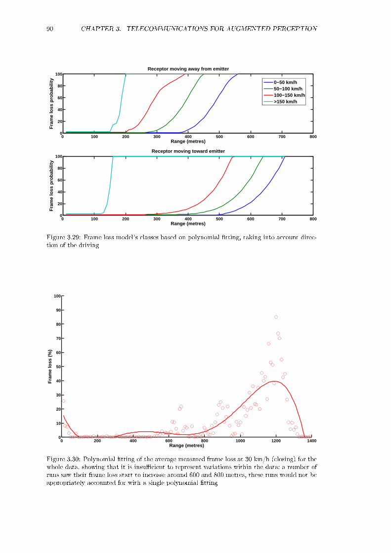
90 CHAPTER 3. TELECOMMUNICATIONS FOR AUGMENTED PERCEPTION

0 100 200 300 400 500 600 700 8000

20

40

60

80

100

Range (metres)

Fra

me

loss

pro

babi

lity

Receptor moving away from emitter

0 100 200 300 400 500 600 700 8000

20

40

60

80

100

Range (metres)

Fra

me

loss

pro

babi

lity

Receptor moving toward emitter

0−50 km/h50−100 km/h100−150 km/h>150 km/h

Figure 3.29: Frame loss model's classes based on polynomial tting, taking into account direc-tion of the driving

0 200 400 600 800 1000 1200 14000

10

20

30

40

50

60

70

80

90

100

Range (metres)

Fra

me

loss

(%

)

Figure 3.30: Polynomial tting of the average measured frame loss at 30 km/h (closing) for thewhole data, showing that it is insucient to represent variations within the data; a number ofruns saw their frame loss start to increase around 600 and 800 metres, these runs would not beappropriately accounted for with a single polynomial tting

3.7. 802.11P MODELISATION 91

example as seen in 3.6.2, at 30 km/h range varied a lot, from 460 metres in the worst case to

almost 1.4 km in the best case. Trying to get the least squares tted upon the average frame

loss measured in these conditions would result to something akin to Fig. 3.28. Obviously, this

does not model real performance. Using a noise envelop around the average tting would not

yield better results. Indeed, unless the noise keeps a memory of its previous realisations, the

frame loss probability at two consecutive discretised ranges (e.g. every 10 metres) could jump

to very dierent values. This does not correspond to the behaviour we have measured.

3.7.3 Frame loss proles logistical model

In order to compensate for the disadvantages in the polynomial tting, another approach is

needed; it is a requirement that it can simulate a large variability of performances and include

sources of defects like multi-path reections from the ground, objects and vegetation, weather,

and hardware inhomogeneities. This means being able to simulate conditions from the worst

case, barely 200 metres of range, to the best case, more than one kilometre, while remaining

consistent over the time window while the two nodes are connected.

To do so, we decided to use an approach we named frame loss proles. A prole represents a

single uninterrupted connection between two IVC devices and is used to determine the frame

loss probability at any given distance, as long as they are within range (that is, as long as frame

loss is under 100%). In using proles we focus on modelling individual measurement runs rather

than the average frame loss as shown for all runs in Fig. 3.23; thus, by generating dierent

proles we can cover the large performance variations we measured. This approach also allows

a temporally consistent frame loss probability and avoid unrealistic probability shifts at two

consecutive distances that could arise from using a simple average-plus-noise model of the

whole measurement. It is important to note however that although they are accounted for in

the model, the sources of performance variations cannot be dierentiated, nor can their relative

importance be modied.

3.7.3.1 Individual frame loss proles

A frame loss prole τ is described by equation 3.2:

τ = A. expB.(d−C)2

+exp (D.d+ E)

1 + exp (D.d+ E)(3.2)

where d is the distance between the emitter and receptor; and A,B, . . . E are parameters es-

timated from empirical data. τ is the addition of two models, as illustrated in Fig. 3.31. An

instance of a prole compared to an individual measurement run is shown in Fig. 3.33.

Term A. expB.(d−C)2

represents the frame loss area corresponding to the strongest ground re-

ection interferences, centred at distance C. At this point the ground-reected signal is strong

enough to cancel out a large proportion of the incoming direct signal's energy, pushing a pro-

portion of frames under the reception threshold of the chipset; the frame loss corresponding to

this proportion is represented by A. The width of the bell curve is in proportion to B; note

that B is always negative. The model assumes that no counter-measure is applied to reduce

the frame loss induced by interferences at C.

The Friis transmission equation, modied to account for ground reections, can be used to

theoretically conrm the value of C. Assuming a dry concrete ground and realistic antenna

92 CHAPTER 3. TELECOMMUNICATIONS FOR AUGMENTED PERCEPTION

0.1

0.5

0.9

Range (metres)

Fra

me

loss

rat

io

modelbell curvelogistical regression

C

A

prop. to −B

−E/D

4/D

Figure 3.31: Decomposition of a frame loss prole τ , with its parameters

60 80 100 120 140 160 180−85

−80

−75

−70

−65

−60

−55

Range (metres)

Sig

nal s

tren

gth

(dB

m)

60 80 100 120 140 160 1800

0.005

0.01

0.015

0.02

0.025

0.03

0.035

Den

sity

Theoritical received signal strength Low speedIntermediate speedHigh speed

Figure 3.32: Distribution of parameter C (the central distance of strongest ground reectioninterferences) for the three speed classes (right axis), compared to the received signal strengththeoretical value (left axis)

3.7. 802.11P MODELISATION 93

0 100 200 300 400 500 6000

0.1

0.2

0.3

0.4

0.5

0.6

0.7

0.8

0.9

1

Range (metres)

Fra

me

loss

rat

io

Actual measurementFrame loss profile

Figure 3.33: Comparison of a frame loss prole versus the corresponding actual measurement

heights, the Friss equation yields the received signal lowest strength at a distance of 120 metres.

The probability densities for the location of C are shown in Fig. 3.32, together with the

theoretical value computed with the Friss equation. Factors such as speed, vehicle body shape,

altitude prole of the track and pitch variations, explain that C is not always recorded at the

same distance.

Term exp(D.d+E)1+exp(D.d+E) is a logistical regression where the log-odds of τ is modelled linearly as

a function of distance d. This term represents the progressive increase of frame loss as the

received signal strength decreases. D and E by themselves have no direct physical meaning;

however, the ratio −ED corresponds to the distance from the emitter at which the average frame

loss passes over 50%. Similarly, 4D expresses the distance between the 10% and 90% frame loss

thresholds.

3.7.3.2 Frame loss proles classes

We created three classes, which are classied according to the relative speed between the emitter

and receptor. Since the measurements have shown that the direction of movement is not an

actual inuence on 802.11p performance, it is not used in this model. The classes are:

speed = [0; 50] , [50; 100] , [100; 150]

The model's parameters A,B, . . . E are estimated on the 2011 dataset using the Levenberg-

Marquardt algorithm for non-linear least squares [95], for each class. Experimental data show

that D and E are linearly correlated. The other parameters are assumed to be independent.

The relationship between D and E is given by a Generalised Linear Model regression from the

observed values of D and E:

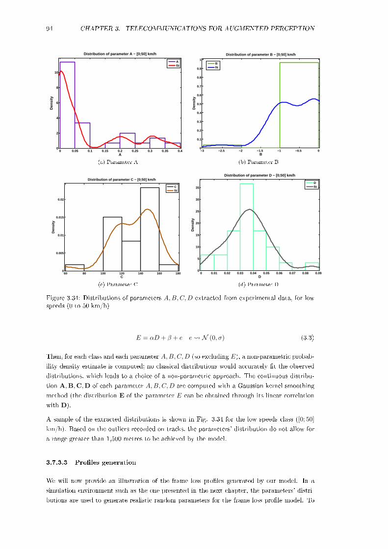
94 CHAPTER 3. TELECOMMUNICATIONS FOR AUGMENTED PERCEPTION

0 0.05 0.1 0.15 0.2 0.25 0.3 0.35 0.40

2

4

6

8

10

A

Den

sity

Distribution of parameter A − [0;50] km/h

Afit

(a) Parameter A

−3 −2.5 −2 −1.5 −1 −0.5 00

0.1

0.2

0.3

0.4

0.5

0.6

0.7

0.8

0.9

1

B

Den

sity

Distribution of parameter B − [0;50] km/h

Bfit

(b) Parameter B

60 80 100 120 140 160 1800

0.005

0.01

0.015

0.02

C

Den

sity

Distribution of parameter C − [0;50] km/h

C fit

(c) Parameter C

0 0.01 0.02 0.03 0.04 0.05 0.06 0.07 0.08 0.090

5

10

15

20

25

30

35

D

Den

sity

Distribution of parameter D − [0;50] km/h

D fit

(d) Parameter D

Figure 3.34: Distributions of parameters A,B,C,D extracted from experimental data, for lowspeeds (0 to 50 km/h)

E = αD + β + e e N (0, σ) (3.3)

Then, for each class and each parameter A,B,C,D (so excluding E), a non-parametric probab-

ility density estimate is computed; no classical distributions would accurately t the observed

distributions, which leads to a choice of a non-parametric approach. The continuous distribu-

tion A,B,C,D of each parameter A,B,C,D are computed with a Gaussian kernel smoothing

method (the distribution E of the parameter E can be obtained through its linear correlation

with D).

A sample of the extracted distributions is shown in Fig. 3.34 for the low speeds class ([0; 50]

km/h). Based on the outliers recorded on tracks, the parameters' distribution do not allow for

a range greater than 1,500 metres to be achieved by the model.

3.7.3.3 Proles generation

We will now provide an illustration of the frame loss proles generated by our model. In a

simulation environment such as the one presented in the next chapter, the parameters' distri-

butions are used to generate realistic random parameters for the frame loss prole model. To

3.7. 802.11P MODELISATION 95

generate sets of parameters, the inverse transform sampling method is used. The A,B,C,D

distributions for each class are transformed into cumulative distribution functions Gx where

x ∈ A,B,C,D. These cumulative distributions are then used as follows:

1. For each x ∈ A,B,C,D // x is a parameter and x its distribution

(a) u← U(0, 1) // a random number u is generated from the uniform distribution U(0, 1)

(b) x← G−1x (u) // a parameter receives the value from its inverse cumulative distribu-

tion

2. End For

3. E ← αD + β + e // E is obtained from the linear relationship that links it to D, where

α and β are the regression parameters and e is the Gaussian noise e N (0, σ)

4. τ = A. expB.(d−C)2

+ exp(D.d+E)1+exp(D.d+E) // Once each parameter has been assigned a value, τ

can be processed from the values with Eq. (3.2)

Fig. 3.35a shows the range that our model can achieve in generating individual frame loss

proles; each curve is a single dierent drawing of u for the parameters. The ground-reection

interference remain concentrated around the 120-metre mark (as shown in the zoomed-in graph

from 3.35b), and the rising part shows a large range of variability: the best case prole allowed

an error-free connection between two nodes until almost 1,000 metres, while on the other hand

the worst case prole did not even return to a very low loss probability (i.e. less than 5%) after

passing the ground interference area, yielding a total range of barely 300 metres.

Each individual prole represent a set of specic conditions that could be found on the road; a

prole can represent realistic conditions on a sunny or on a rainy day. Changing the paramet-

ers of the Gaussian kernel smoothing method allows generating distributions for the model's

parameters that either closely reproduce experimental data or, on the other hand, allow non-

measured but plausible proles.

In Fig. 3.36a, we show the distribution of the point at which frame loss reaches 50%, expressed

in our model as the ratio −ED , obtained for 1,000 prole generations. The inuence of relative

speed on frame loss (and range) is clear, as the bulk of generated proles shift from a relatively

uniform distribution towards being concentrated in the 200 to 400-metre interval. Similarly, in

Fig. 3.36b we show the distribution of C, the point of maximum ground-reection interference,

as obtained for 1,000 prole generations in each class.

However, this logistical model has a few limitations. Most of the distributions are estimated

independently of each other (they are not correlated), which can lead to the generation of

parameters whose values are independently realistic, but combination is unlikely. One must

decided beforehand what is deemed an acceptable level of innovation from the model regarding

the experimental data.

The most important limitation however, is found in an average trailing eect that takes place

at large range values, when the average of many proles are considered. When comparing the

average frame loss obtained from many prole generations with the average experimental frame

loss (see Fig. 3.41), one notices that the model does not reach a 100% frame loss until very

large range values, compared to the measured data. This trailing arises from the asymptotic

nature of term exp(D.d+E)1+exp(D.d+E) , and means that there is a non-zero probability of letting some

96 CHAPTER 3. TELECOMMUNICATIONS FOR AUGMENTED PERCEPTION

0 500 1000 15000

0.1

0.2

0.3

0.4

0.5

0.6

0.7

0.8

0.9

1

Range (metres)

Fra

me

loss

pro

bab

ility

(a) Frame loss proles generated with 100 drawings of u

50 100 150 2000

0.05

0.1

0.15

0.2

0.25

0.3

0.35

0.4

0.45

0.5

Range (metres)

Fra

me

loss

pro

bab

ility

(b) Zoom on the frame loss peaks caused by ground-reection interferences, for 12 drawings of u

Figure 3.35: Generation of frame loss proles for the [50;100] km/h class

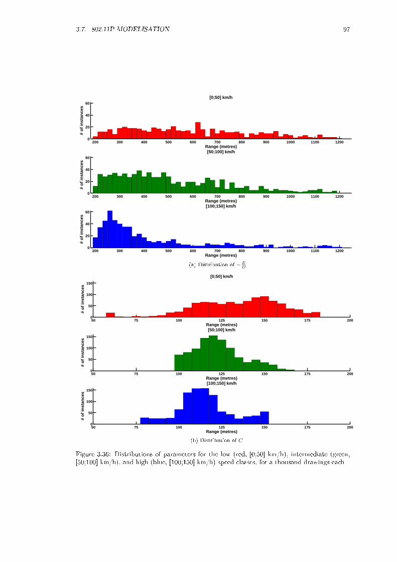
3.7. 802.11P MODELISATION 97

200 300 400 500 600 700 800 900 1000 1100 12000

20

40

60

Range (metres)

# o

f in

stan

ces

[0;50] km/h

200 300 400 500 600 700 800 900 1000 1100 12000

20

40

60

Range (metres)

# o

f in

stan

ces

[50;100] km/h

200 300 400 500 600 700 800 900 1000 1100 12000

20

40

60

Range (metres)

# o

f in

stan

ces

[100;150] km/h

(a) Distribution of −ED

50 75 100 125 150 175 2000

50

100

150

Range (metres)

# o

f in

stan

ces

[0;50] km/h

50 75 100 125 150 175 2000

50

100

150

Range (metres)

# o

f in

stan

ces

[50;100] km/h

50 75 100 125 150 175 2000

50

100

150

Range (metres)

# o

f in

stan

ces

[100;150] km/h

(b) Distribution of C

Figure 3.36: Distributions of parameters for the low (red, [0;50] km/h), intermediate (green,[50;100] km/h), and high (blue, [100;150] km/h) speed classes, for a thousand drawings each

98 CHAPTER 3. TELECOMMUNICATIONS FOR AUGMENTED PERCEPTION

C (F−E)/D (1−E)/D0

1

F

A

Range

Fra

me

loss

rat

io

profilelinear partbell curve

prop. to −B

Figure 3.37: Decomposition of a frame loss prole τ , with its parameters

frames pass at innite ranges. Innite ranges can be avoided by forcing the frame loss prole

at 100% past a certain range threshold (typically 1,500 metres), but it can be argued that it

is a relatively non-elegant solution. However, a small probability that a frame passes at more

than 1 km in some classes will, where no experimental data showed such a behaviour.

3.7.4 Frame loss proles semi-linear model

In order to compensate for the non-zero transmission success probability produced by logistical

frame prole model, we rened our approach to ensure that the frame loss does reach 100%

within the maximum range measured during our on-track experiments. Instead of having a

logistical regression-based second term, we now use a linear second term.

3.7.4.1 Individual Frame Loss Proles

In this new version of the model, a single frame loss prole τ is now described by:

τ = max[A. expB.(d−C)2

; min (max [D.d+ E;F ] ; 1)]

(3.4)

where d is still the distance between the emitter and receptor; and A,B, . . . F are the model's

new parameters. The new frame prole shape is illustrated on Fig. 3.37. Term A. expB.(d−C)2

is the same as in the logistical model. The new term D.d+ E is a linear regression where τ is

modelled linearly as a function of distance d and parameters D and E. This term represents the

progressive increase of frame loss as the received signal strength decrease. The increase starts

from a non-zero frame loss ratio value given by parameter F , which represents the average small

perturbations measured within range. Typically, F will be low (less than 5%). D and E have

two meaningful ratios: ratio F−ED gives the distance at which frame loss starts to increase from

the plateau at F ; ratio 1−ED expresses the distance at which frame loss reaches 100%, hence

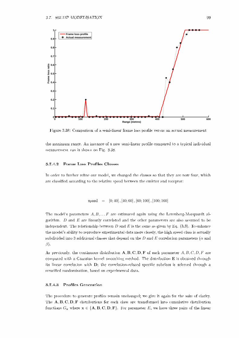
3.7. 802.11P MODELISATION 99

0 100 200 300 400 500 6000

0.1

0.2

0.3

0.4

0.5

0.6

0.7

0.8

0.9

1

Range (metres)

Fra

me

loss

rat

io

Frame loss profileActual measurement

Figure 3.38: Comparison of a semi-linear frame loss prole versus an actual measurement

the maximum range. An instance of a new semi-linear prole compared to a typical individual

measurement run is shown on Fig. 3.38.

3.7.4.2 Frame Loss Proles Classes

In order to further rene our model, we changed the classes so that they are now four, which

are classied according to the relative speed between the emitter and receptor:

speed = [0; 40] , [40; 60] , [60; 100] , [100; 160]

The model's parameters A,B, . . . F are estimated again using the Levenberg-Marquardt al-

gorithm. D and E are linearly correlated and the other parameters are also assumed to be

independent. The relationship between D and E is the same as given by Eq. (3.3). To enhance

the model's ability to reproduce experimental data more closely, the high speed class is actually

subdivided into 3 additional classes that depend on the D and E correlation parameters (α and

β).

As previously, the continuous distribution A,B,C,D,F of each parameter A,B,C,D, F are

computed with a Gaussian kernel smoothing method. The distribution E is obtained through

its linear correlation with D; the correlation-related specic subclass is selected through a

stratied randomisation, based on experimental data.

3.7.4.3 Proles Generation

The procedure to generate proles remain unchanged; we give it again for the sake of clarity.

The A,B,C,D,F distributions for each class are transformed into cumulative distribution

functions Gx where x ∈ A,B,C,D,F. For parameter E, we have three pairs of the linear

100 CHAPTER 3. TELECOMMUNICATIONS FOR AUGMENTED PERCEPTION

regression coecients αi, βi, where i ∈ 1, 2, 3 and a discretised cumulative distribution H,

so that:

H (1) = ψ

H (2) = ω

H (3) = 1

where ψ, ω ∈ [0; 1]2and ψ ≤ ω , which represent the relative weight of each correlation regime

(subclass) in the experimental data. These cumulative distributions are then used as follows:

1. For each x ∈ A,B,C,D, F // x is a parameter and x its distribution

(a) u← U(0, 1) // a random number u is generated from the uniform distribution U(0, 1)

(b) x← G−1x (u) // a parameter receives the value from its inverse cumulative distribu-

tion

2. End For

3. v ← U(0, 1) // a random number v is generated from the uniform distribution U(0, 1)

4. i← H−1(v) // i takes the value from the inverse cumulative distribution

5. α, β ← αi, βi// the pair of coecient that corresponds to the value of i is selected

6. E ← αD+ β + e // E is obtained from the linear relationship that links it to D, e is the

Gaussian noise e N (0, σ)

7. τ = max[A. expB.(d−C)2

; min (max [D.d+ E;F ] ; 1)]// Once each parameter has been

assigned a value, τ can be processed from the values with Eq. (3.4)

Fig. 3.39a shows the range of variations achieved by the new semi-linear model in the [60; 100]

class. By computing the average of many generated proles we obtain curves that accurately

reproduce the average measurements, as shown in Fig. 3.40 for the averages of a thousand

proles of each class. Fig. 3.41 shows how the semi-linear model improves on the logistical one

(the intermediate speeds class is shown).

Thus, the semi-linear model solves the trailing eect that was problematic with the logistical

model, and shows that with an appropriate set of parameters, the model can closely reproduce

experimental data. It remains possible to obtain more diversity by adapting the Gaussian kernel

smoothing method, as recommended for the logistical model.

In a simulated environment, a prole can be generated each time a connection is established

between 2 nodes (typically when it enters within a static maximum range threshold); one emitter

can have several proles active at the same time if it is connected to more than one receptor.

Some limitations remain with this new model. At rst, there is no way of knowing which

conditions eects a particular prole. If two neighbouring vehicles are connected to the same

emitter, it is possible that one vehicle has a prole corresponding to dry, sunny weather while

the other has humid, overcast conditions. Secondly, the model's user cannot select a specic

type of inuence, such as weather (the only way to do so would be to include sub-classes that

would have their own distributions of A,B, . . . F ). Small correlations between other parameters

than D and E have not been investigated and might still have an eect on the overall model.

3.7. 802.11P MODELISATION 101

0 100 200 300 400 500 600 700 800 900 10000

0.1

0.2

0.3

0.4

0.5

0.6

0.7

0.8

0.9

1

Range (metres)

Fra

me

loss

pro

bab

ility

(a) Frame loss proles generated with 100 sets of drawings of u

50 100 150 2000

0.05

0.1

0.15

0.2

0.25

0.3

0.35

0.4

0.45

0.5

Range (metres)

Fra

me

loss

pro

bab

ility

(b) Zoom on the frame loss peaks caused by ground-reection interferences, for 100 sets of drawings of u

Figure 3.39: Generation of frame loss proles for the [60;100] km/h class

102 CHAPTER 3. TELECOMMUNICATIONS FOR AUGMENTED PERCEPTION

0 200 400 600 800 10000

0.2

0.4

0.6

0.8

1

Range (metres)

Fra

me

loss

rat

io

Very low speeds

0 200 400 600 800 10000

0.2

0.4

0.6

0.8

1

Range (metres)

Fra

me

loss

rat

io

Low speeds

0 200 400 600 800 10000

0.2

0.4

0.6

0.8

1

Range (metres)

Fra

me

loss

rat

io

Intermediate speeds

0 200 400 600 800 10000

0.2

0.4

0.6

0.8

1

Range (metres)

Fra

me

loss

rat

io

High speeds

Figure 3.40: Averages of 1,000 proles for each of the four classes, compared to the measuredaverages (in black)

0 100 200 300 400 500 600 700 800 900 10000

0.1

0.2

0.3

0.4

0.5

0.6

0.7

0.8

0.9

1

Range (metres)

Fra

me

loss

rat

io

Experimental average frame lossLogistical modelSemi−linear model

Figure 3.41: Comparison of the averages for the experimental data and the two models (forclass [60; 100] km/h)

3.8. CONCLUSION 103

3.8 Conclusion: inuence of 802.11p limitations on aug-

mented perception and safety applications

In this chapter, we have extensively discussed the results of an empirical performance evaluation

of 802.11p, with a focus on supporting higher-level CS safety applications. Data from this

evaluation was used to build a new empirical model that will be utilised in the following chapters,

to support our CS simulation architecture and, eventually, augmented perception. However,

we must now discuss the consequences of the results from our evaluations, on upper layers of a

cooperative architecture. The performance attainable by 802.11p strictly limits the performance

one gets from an augmented map, or any other type of applications expected to use remote

information shared through wireless telecommunications.

Range showed a strong dependency on the relative speed between the emitter and the receptor.

Frame loss follows the same trend, since frame loss and range are related. The best ndings

from our investigations concerns latency. Indeed, we have found that latency depends on the

size of the data exchanged. For 100 bytes MAC frames, latency remains under 4 milliseconds in

almost all circumstances, regardless of range and relative speed. Relative speed did not show any

inuence, and range mattered only when close to maximum range, as ad-hoc mode mechanisms

started to delay the transmission of frames. Note that large frames will probably be aected

in these conditions and fare worse than the smaller frames we used for our measurements.

While it might not change much for smaller frames, the specic OCB mode that was created

for 802.11p will likely extend the range compared to ad-hoc mode. Indeed, frames sent with

the OCB mode should oer, given the same exact hardware set-up, similar performance as

management frames. Our measurements have shown that management frames (beacons) could

be picked up, up to 200 metres further than normal frames in some settings.

A trend that emerged from the analysis of our data is that a lot of previous studies must have

overestimated the performance of 802.11p, our results being more pessimistic than existing

literature in most cases. We used a fairly low-cost set-up, which is typically what automotive

manufacturers will want to have before CS start getting deployed on the road. We believe

our implementation is not a deployment-worthy one. Yet, it is likely that the only major

dierence between our setup and actual ones in the future, is the antenna. We were limited

by hardware availability, and had to use stick antennas, which are unlikely to be deployed on

the road (but for some very specic cases). As shown in previous research [93, 86, 81] and our

own results, antennas are important. If combined with the vehicle's body eects, the quality

of antennas led to range variations amounting up to 500 metres, and explained a perceived

directivity in maximum transmission range. We can condently argue that it explains some

unexpected ndings from previous studies, notably the very directivity from [83]. Nonetheless,

these hardware inhomogeneities alone cannot explain the total performance variability that

was measured. Some arose from meteorological conditions, such as the relative air humidity,

while others have sources that remain unidentied. A particularly infamous phenomenon was

the capture blindness that we experienced many times. The receptor vehicle was unable to

pick-up frames sent by the static emitter until it was less than 50 metres away, while nothing

had changed from previous experimental runs.

Based on these measurements, we propose a new, simple approach to build an application-

oriented model of 802.1p performance. This model has the advantage of taking into account all

the variations we discussed above, and to also reproduce their relatively unpredictable beha-

104 CHAPTER 3. TELECOMMUNICATIONS FOR AUGMENTED PERCEPTION

viour. This model, we believe, bridges the gap between physical layer and network models by

providing a focus on some simple, yet central, performance indicators for 802.11p in small-to-

medium sized networks. It will be entirely focused on delivering realistic performance indicators

to upper-layer CS simulations. It will also form the basis of our CS simulation architecture de-

scribed in Chapter 4, and the augmented map building approach from Chapter 5 onwards.

What do the present chapter's ndings say in terms of limitations for augmented perception?

In Mourllion [31], the author recommends an augmented map covering a radius of 500 metres

around the ego-vehicle. Within the context of their study, this value applies to a freeway

context, and is probably too large for an urban setting. At 130 km/h, 500 metres corresponds

to approximately 15 seconds, which is a reasonable timeframe for safety applications. However,

given our data, the range of actually achieving communication with other vehicles and RSUs for

an ego-vehicle driving on a freeway will vary widely. Indeed, connectivity range with RSUs will

be relatively limited. With a frame loss threshold of 25%, reliable connection will be established

with the RSUs only 400 metres ahead of it. In most cases, frame loss will be lower than 5% only

within 250 metres of the RSUs. Connectivity with vehicles driving in the opposite direction is

even worse, as their relative speed is largely above 200 km/h. In that case, range will shrink

to values which are close to 802.11g/n specications, that is: 150-250 metres. However, the

ego-vehicle will still be able to achieve long range communications with a vehicle driving in the

same direction. This might be used to compensate for the limited connectivity with RSUs and

counter-driving vehicles, by using relaying schemes.

The inuence of these limitations on safety applications will depend on the applications' specic

goals. On an freeway, a vehicle-hosted collision warning application will likely be able to perform

well, within Mourllion's augmented map radius, as there is no requirement to connect to counter-

driving vehicles or to RSUs, especially if the percentage of equipped vehicles is large enough.

However, an exit/entry ramp monitoring application hosted on a RSU might nd it more useful

to use a range of other exteroceptive sensors rather than rely on 802.11p. In a suburban setting,

where relative speeds will be lower, 802.11p performance will be better, although non-LoS will

have to be considered there.

In conclusion, 802.11p-based telecommunication have the necessary qualities to support CS in

general, and augmented map building in particular, but developers must be cautious about the

expected performance. They specically need to account for the possibility that performance

can degrade quickly and in an unexpected manner. We will remain cautious of this fact for

the remainder of this research, which calls for using robust data fusion methods to build the

augmented map.

Summary of chapter's contributions

Outcomes

An open-source 802.11p IVCD was successfully deployed on vehicles.

A comprehensive evaluation of 802.11p IVC was performed on track in a close-to-

real-road setting.

An empirical model of key 802.11p performance metrics was developed.

Key ndings

3.8. CONCLUSION 105

802.11p performance was worse than expected in terms of range.

Range (and frame loss) showed a strong dependence on the relative speed between

an emitter and a receptor.

Fluctuations of up to 500 metres were possible depending on the quality of the

antenna.

Latency was limited, and remained stable regardless of speed or range.

Limitations

The measurements did not account for the presence of other vehicles, IVC-equipped

or not.

Latency was measured principally for smaller frames, the scope of measurements

with larger frames remained limited.

The specic outside of BBS context mode for 802.11p was not used.

The 802.11p model is not adapted for VANETs of more than a few vehicles.

106 CHAPTER 3. TELECOMMUNICATIONS FOR AUGMENTED PERCEPTION

Chapter 4

Simulation architecture for

Cooperative Systems applications

4.1 Introduction

The previous chapter discussed the limitations of the most common telecommunication techno-

logy used to support Cooperative Systems (CS). It demonstrated how the theoretical perform-

ance of 802.11p has been overestimated. Indeed, if simple and inexpensive hardware is allowed

to achieve performance strong enough to support potential safety-critical CS applications, care

had to be taken in some settings. Notably, we showed that the range reduction linked to high

relative speeds suppress any range advantage that telecommunications could have on exclus-

ively mono-vehicle sensors. The previous chapter then built an empirical model of 802.11p.

To support this model, we argued that we needed a modelisation of performance metrics that

were the most relevant to higher-level simulations of CS application. Such simulations aim at

studying the benets of CS application, notably for road safety, without having to account for

ner details in the underlying network layers; this is the research methodology that was chosen

at the conclusion of Chapter 2.

The aim of the present chapter is to design and build a simulation architecture that can support

higher-level CS applications. It should be generic enough to be used to support studies on

many dierent types of CS applications, including but not limited to augmented perception.

Demonstrating the simulation architecture's usefulness will be a two-tiered process; (1) at rst,

our goal will be to show that previous results on the safety benets of IVC can be validated

using the architecture; then (2) our goal will be to test whether these results still hold when the

simulation's realism is increased. Building such an architecture relates to the following research

questions outlined in Chapter 1:

1. Can an augmented map-based risk assessment system be more ecient than a similar

non-cooperative system?

2. What are augmented perception limitations, given current technology in embedded com-

puting and telecommunications?

Chapter 3 has partially answered the second question by addressing the issue of telecommunica-

tions limitations. The present chapter will provide the framework within which further answers

108 CHAPTER 4. SIMULATION ARCHITECTURE FOR CS APPLICATIONS

will become achievable.

Indeed, the architecture designed in the present chapter will be used within this thesis as the

core framework in which research on augmented perception will take place. In Chapter 3, we

argued that before looking into CS, it was necessary to study the performance of their underlying

level, telecommunications, in the road environment. Similarly, in the present chapter, we must

rst build a realistic simulation environment before any meaningful research on augmented

perception can be undertaken. The CS simulation architecture was built by taking advantage of

the multiple functionalities of the SiVIC simulator and the RTMaps multi-sensors prototyping

platform. This architecture is very versatile and can be used to simulate a wide variety of on-

road scenarios. Its principal contribution is to increase the degree of realism for CS simulations,

notably by incorporating the 802.11p IVC model developed in Chapter 3. As mentioned before,

it will provide an environment within which augmented perception will be built and evaluated.

As such, it is a second important stepping stone toward augmented map construction.

However, before addressing augmented perception in the next chapter, we will rstly discuss

results related to the safety benets of CS, by considering only our reference scenario (the

vehicles string). This will allow us to demonstrate the usefulness and interest of our simulation

architecture outside of augmented perception per se, with an EEBL application of increasing

complexity.

Since the aim of this chapter is to develop a CS simulation architecture to study safety-orientated

cooperative applications which includes augmented perception, it makes sense to use a reference

scenario that is not too complex and where CS safety benets can be immediately veried by

acting on only a limited set of parameters. Indeed, thanks to this relatively simple scenario,

there have been a number of studies on the safety benets of introducing IVC inside strings of

vehicles. So far, these results have been generally positive, showing that even a limited amount

of cooperative vehicles was enough to decrease crashes and by extension, reduce road fatalities.

A more detailed description of these results was provided in Chapter 2.

In the rst part, we show that we can reproduce results from previous simulations with a

simple version of the EEBL scenario within our simulation framework. However, many of these

previous simulations make important assumptions on the telecommunication's performance or

limit the realism of the string's behaviour (for example, by having strings of regularly spaced

homogeneous vehicles). In the second part, we use a more realistic scenario with strings that

dier at each run. Our architecture allows studying ner details than generally available in other

comparable simulations, which has allowed us to obtain unexpected new results regarding some

of the criteria used to assess the safety benets of EEBL. They show that EEBL might actually

not decrease the severity of rear-end collisions, even though the actual number of such collisions

is reduced.

Chapter Outline

The rst section presents the rationale and motivation for building a CS simulation architecture

in great detail, notably outlying the requirements for an accurate simulation of Cooperative

applications.

Then, the second section presents the design of our CS simulation architecture. Firstly, it intro-

duces the software that enables our architecture (further details are available in the appendices).

Next, it explains its design in detail, and provides a validation to our implementation. In the

4.1. INTRODUCTION 109

third section, the architecture's validation is achieved by reproducing previous results using our

architecture.

The fourth section discusses the improvements enabled by our architecture. In the rst instance,

it presents how our architecture can be used to study CS usage scenarios with a high degree

of granularity, notably by extending on the scenario used for validation. Then, we discuss new

results that have emerged from simulating EEBL. It shows that some, not all, safety benets of

EEBL may have been overestimated with previous simulations, especially regarding the safety

criterion based on the severity of collisions.

Lastly, the fth section closes this chapter with a summary of its main contributions and

ndings.

110 CHAPTER 4. SIMULATION ARCHITECTURE FOR CS APPLICATIONS

Rationale: a complex CS simulation architecture for close-to-reality simulation

In Chapter 2, we discussed why the relative failure of an on-road implementation of an EEBL

system warranted a focus on simulations to study the limitations or the eectiveness of CS,

specically the vehicles string scenario. In this section, we will discuss the rationale behind

developing an improved simulation architecture that is generic enough to be used to support

studies on many types of CS applications, including but not limited to, the vehicles string

scenario and augmented perception.

Advanced simulation architectures or platforms are highly desirable for CS. Indeed, develop-

ing CS requires additional resources, notably in terms of telecommunication and perception

hardware, which are both time consuming and expensive. Therefore, it is essential to have

a simulation environment or platform that allows prototyping and evaluating extended, en-

riched and cooperative Advanced Driver Assistance Systems (ADAS) in the early stages of

the system's design. There are many ways prototyping and evaluation can be undertaken, for

example, developers might want to test the eectiveness of an anti-collision application at an

intersection under a number of dierent trac conditions. Or, they might want to test its

robustness to changing meteorological conditions. For that, a virtual simulation platform has

to integrate models of various road environments, virtual on-vehicle sensors (proprioceptive &

exteroceptive), infrastructure-based sensors and IVC devices, which are all consistent with the

laws of physics. Similarly, a physics-based model for vehicular dynamics coupled with actuators

(steering wheel angle, torques on each wheel) is required to maximise realism. By using such

a platform, it becomes possible to accurately simulate the performance of future cooperative

ADAS within a realistic environment.

We concluded in Chapter 2 that it was warranted to improve existing simulations of the vehicles

string scenario in order to study the benets of EEBL in a more realistic environment. Such

an eort should also lead to the creation of a platform that meet the requirements outlined

in the previous paragraph, where augmented perception can be studied, as well as any other

type of cooperative application. So, our aim shall be to develop an architecture that can

simulate and evaluate CS applications in a broader context, to continue on verifying the safety

benets of EEBL (such as in [22, 23]) and to enable the accurate simulation of complex systems

featuring augmented perception. Eventually, this architecture should be able to support the

development of actual CS applications that will be deployed on the road, for prototyping like

we did in Chapter 2 or for actual commercial use.

The proposed architecture builds upon the SiVIC-RTMaps interconnected platform function-

alities [28, 96] to meet performance and realism requirements. Our CS simulation architecture

will bring several improvements to the SiVIC-RTMaps coupling, notably IVC as well as vehicle

control. The principal change is the extension to the existing transponder-like IVC simulation

in SiVIC [97] using the 802.11p empirical model we created in Chapter 3. This allows simulat-

ing small-scale networks of IVC-equipped vehicles and RSUs on a freeway, rural or suburban

context. In order to have a real-life simulation of a human driver as well as introducing mech-

anisms related to CCW like emergency braking manoeuvres, several improvements are made to

the vehicle's controllers compared to previous versions. Having realistic vehicle motion model

and controllers are important, as some CS safety-orientated applications need to act on the

vehicle's behaviour to perform their task. For example in the vehicles string scenario, it is

important to have a realistic braking model to simulate emergency braking manoeuvres. We

will present the architecture's dierent modules, including supporting platforms such as SiVIC

in further detail in section 4.2.

4.1. INTRODUCTION 111

Within this chapter, the main goal of our architecture is to evaluate the impact of introducing

IVC devices into a driving situation that can lead to crashes, compared to using non-cooperative

ADAS or without any ADAS altogether. To demonstrate that we can obtain meaningful results,

we will show how an EEBL application can be simulated with it, using the reference vehicles

string scenario. This will happen in two stages.

Firstly, in order to validate our approach, we have found that our application reproduces results

from the previous larger scale simulations [22, 23] (see 4.3) using a simplied scenario. Secondly,

some new results have emerged by using a more realistic scenario (see 4.4). Indeed, we evalu-

ated the severity of crashes, via the computation of the Equivalent Energy Speed (EES, more

details on how to compute it are given 4.3.3), from several hundred runs of our own simulation.

If introducing IVC decreases the number of crashes as expected, the average EES does not

decrease. This means that the severity of the remaining crashes remain constant, whatever the

percentage of IVC-equipped vehicles are.

These results raises a few concerns about the actual safety benets of EEBL in particular, and

IVC or CS in general. It is often assumed that IVC can help in reducing the severity of crashes

(notably for the vehicles string scenario in Mourllion [31]), and in some cases it might be more

benecial to favour this eect rather than focusing on reducing crash numbers (a practice called

crash mitigation or pre-crash braking). Our results do not invalidate the benets of EEBL, as we

did get a signicant reduction of collisions when IVC was randomly distributed in the vehicles

string with an increased equipment percentage. However, our results suggest that the eciency

of an EEBL application in reducing the severity of the crashes might have been overestimated

by studies such as [22, 23]. These results are discussed in more details in 4.4 and 4.5.

112 CHAPTER 4. SIMULATION ARCHITECTURE FOR CS APPLICATIONS

4.2 CS/EEBL simulation architecture design

In this section, we will explain the simulation architecture's modules (namely, the V2V/I

802.11p simulation and vehicles controllers), as well as the underlying functionalities of the

SiVIC and RTMaps platforms that support it.

4.2.1 SiVIC-RTMaps interconnection

Our CS simulation architecture is based on the interconnection of the sensors simulation plat-

form SiVIC and the prototyping platform RTMaps. The combined platforms oer many of

the functionalities that are required for advanced simulations of cooperative applications, thus

limiting further additional developments.

SiVIC [28] is a platform designed to enhance the process of developing and evaluating ADAS.

This platform enables the simulation of multi-frequency sensors embedded in static or dynamic

devices, equipments and vehicles commonly used in ADAS. In this context, raw data from

perception systems or actuators systems are substituted by realistic synthesised data or devices.

This functionality is useful for scenarios featuring hazardous environments, complex situations,

or nonexistent or erroneous data (from sensors or actuators). Moreover, data analysis can always

be performed with accurate ground truth references. Initially, the SiVIC platform was built

with the objective of prototyping local perception applications. Since then, ongoing extension

of the platform include the virtual prototyping of control/command or decision algorithms [98]

and CS applications [97].

RTMaps is marketed by Intempora1, based upon work undertaken at Mines ParisTech a

decade ago [94]. Its primary goal is to record and process a large number of simultaneous data

ows such as images, laserscanner scans, positioning data (from GPS, odometer or INS), etc.

User-developed algorithms, for image processing or data fusion for example, can be deployed in

the RTMaps framework in dedicated libraries called packages. Packages themselves contain

components that can apply specic treatments to the data ow. Recorded data can be easily

replayed, which is especially useful to ne tune algorithms with multiple re-runs of the same

on-tracks measurement. The interconnection between SiVIC and RTMaps allows us to replace

real measurements with simulated ones at RTMaps's inputs, creating a fully Software-In-the-

Loop (SIL) development and prototyping approach.

4.2.2 The SiVIC platform

4.2.2.1 Platform's objectives & general functionalities

Many developments aim at improving the safety of road environments through ADAS. These

studies generally take into account an ego-vehicle perception and the corresponding reaction

of the vehicle (e.g. braking and accelerating). However, an ego perception is no longer su-

cient in many situations, as additional information is needed to minimise risk and maximise

driving security. This additional information requires additional resources which are both time

consuming and expensive.

The SiVIC platform is a very ecient tool to develop, prototype and assess high level ADAS

(see Fig. 4.1a), including CS applications. It uses a realistic graphics environment (Fig. 4.1b),

1www.intempora.com

4.2. CS/EEBL SIMULATION ARCHITECTURE DESIGN 113

(a) General architecture of ADAS prototyping with SiVIC

(b) Multiple captures from the Versailles-Satory's test tracks scenery; SiVIC's visual rendering is focused ongenerating accurate image dynamic, rather than merely acceptable realism to human eyes

Figure 4.1: The SiVIC platform

114 CHAPTER 4. SIMULATION ARCHITECTURE FOR CS APPLICATIONS

supported by physically accurate behaviours for vehicles and sensors. It can generate a ow of

time-stamped and synchronised data that can be recorded and/or interacted with by prototyp-

ing and/or data treatment platforms such as RTMaps or Matlab. Furthermore, SiVIC can

generate multiple scenarios with event-driven mechanisms, so that the robustness and reliability

of control and perception algorithms can be extensively tested against many parameters. Thus,

SiVIC can be used, coupled with a platform such as RTMaps, to perform most developments

in a Software-In-the-Loop (SIL) approach, pushing the on-vehicle testing further towards the

end of the development cycle. At this stage, algorithms developed in RTMaps and tested with

SiVIC can be seamlessly integrated into an on-board hardware.

4.2.2.2 Sensors modelling

Proprioceptive and exteroceptive sensors are modelled in SiVIC so that from the point of view

of an algorithm, there is no dierence between a fully SIL sensor and an on-vehicle sensor.

Sensors available in SiVIC are:

Observers that output reference data on an object's position and behaviour

Cameras (can be congured as software or hardware cameras)

Inertial Navigation Systems (3 axes accelerometer + 3 axes gyrometer)

Infrared transmitter (for LoS IVC)

Odometer

Telemetric laserscanner (multi-layered, capable of using either ray-tracing or Z-Buer

methods)

Radiofrequency transponders.

At the time of writing, additional sensors are being implemented in SiVIC which are close

to deployment. Most are related to the implementation of a realistic model of electromagnetic

waves propagation in the platform. They include a GPS simulation that goes up to the inuence

of the satellite's ephemerides and radar. It is the RF transponders, which are used for a CS

application in [97], that are extended here to take advantage of a more realistic model of IVC

behaviour, based on eld measurements. The most advanced electromagnetic systems models

could be used, but unless a perfectly life-like simulation is required, they will generally add

too much processing requirements to a CS-orientated application. Our empirical model has the

advantage of being both realistic and computationally light enough, compared to those lower

level physical models.

4.2.2.3 Vehicles modelling

SiVIC provides a parametric model developed by Sébastien Glaser [99] (see also [100]) for the

dynamic behaviour of the vehicle bodywork on the three axes (roll, pitch and yaw/heading). It

also takes into account the dynamics of shock absorbers and non-linear tyre road forces [101,

102]. Eventually, coupling between longitudinal and lateral axes, the impact of normal force

variations, and alignment of the car are also integrated. The vehicle's chassis is modelled with

an unbending suspended mass. This model allows installing a large number of on-board sensors

4.2. CS/EEBL SIMULATION ARCHITECTURE DESIGN 115

easily. We will use the notations of the chassis dynamics illustrated in Fig. 4.2. This model's

architecture can be enhanced, if necessary, with advanced control chassis such as ESP, ABS or

power train. It is also straightforward enough to install many sensors that will feed observers

(amongst others) and ultimately, control algorithms. Several control modes are available; (1)

human driver; (2) raw trajectory following (discarding many physical limitations of the vehicle);

(3) realistic trajectory following lateral and longitudinal controllers; and (4) external control

from RTMaps or any similar development platform.

Figure 4.2: Dynamic vehicle model

Using a realistic model vehicle as part of our CS simulation architecture is important on many

dierent levels. The simulation must be able to accurately reproduce the vehicle's behaviour

when performing active tasks, such as an automated emergency braking manoeuvre or co-

operative driving/manoeuvring. This is useful as part of the EEBL application which will be

demonstrated later in this chapter. Furthermore, studying augmented perception and, further

on, risk in a given driving simulation, requires that the behaviour of vehicles be reproduced

accurately at both short (less than a second) and medium (up to a few minutes) time scales.

4.2.3 Overall architecture

From the beginning, we developed our CS simulation architecture for EEBL applications, spe-

cically to simulate strings of IVC-equipped vehicles. However, it can be easily expanded and

applied to other scenarios by adding the appropriate modules. Indeed, the architecture is

partially scenario-specic, both in SiVIC and RTMaps:

Scenarios are built in SiVIC using script les that specify the location of objects and many

other parameters such as the environment, type of sensors mounted on vehicles, etc.

The cooperative application itself is developed and implemented in RTMaps in the

form of specic-purpose components. For example in this chapter, it takes the form of a

component, tasked with computing the vehicles' control commands within a set of rules,

inuenced by the trac situation and messages exchanged over a virtual V2V network.

However, developments such as vehicles' control mechanisms (the controller equations them-

selves) and the 802.11p model are not scenario-dependent and are an integral part of SiVIC,

which remains available at all times.

Fig. 4.3 shows the data ow and relationship between the environment, sensors and algorithms.

At the environment level, the dierent objects considered as part of the road includes obstacles

and beacons that belong to the transponder simulation. The road (technically, each segment)

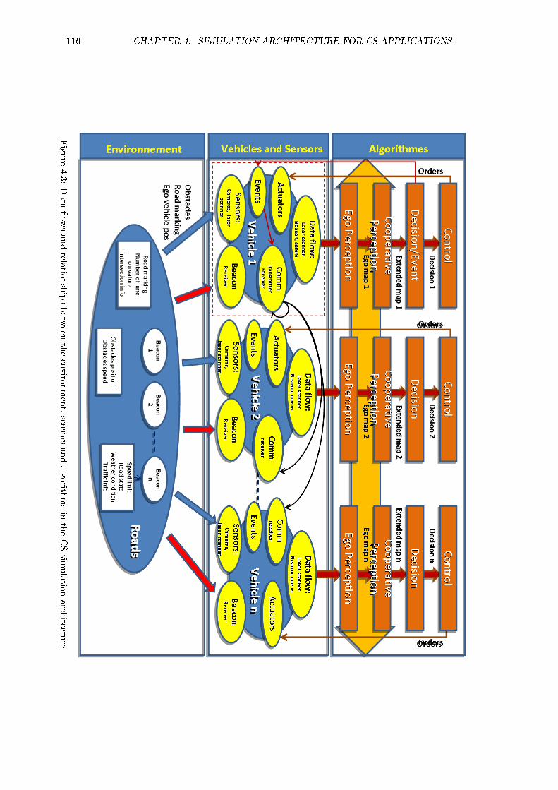
116 CHAPTER 4. SIMULATION ARCHITECTURE FOR CS APPLICATIONS

Figure

4.3:Data

ow

sandrela

tionshipsbetw

eentheenviro

nment,sen

sors

andalgorith

msin

theCSsim

ulatio

narch

itecture

4.2. CS/EEBL SIMULATION ARCHITECTURE DESIGN 117

Figure

4.4:CSsimulationarchitecture'sdetailed

functionsin

SiVIC-RTMaps

118 CHAPTER 4. SIMULATION ARCHITECTURE FOR CS APPLICATIONS

has a set of information that describes its curvature or the number of lanes, amongst other

things. This data is recorded by the sensors embedded on each vehicle. The vehicles also receive

information from the upper layer (algorithms) so that controllers can act upon them.Vehicle

1 is considered the leader and is tted with a transmitter, while the other vehicles (2 to n)

are followers, tted with receptors. Apart from this distinction, each vehicle has identical

features. At the upper layer, a set of algorithms use information sensors to perform a number

of tasks. It is here that most of the user-developed application will be located, for example an

augmented map-building application, which receives information collected by sensors (including

the information that is transmitted via the 802.11p simulation).

The arrows between the middle and upper layer show the data/action chain that occurs when

the EEBL simulation is run. At the onset, data ow is relatively straightforward. Data from

the environment is owed to the decision and control algorithms that compute the commands,

which is then fed back to the actuators so the vehicles maintain a string as specied by the

user. Then, at some point an event is triggered in the leader vehicle (by the decision/event

upper algorithm rst), which starts the emergency braking manoeuvre. New commands are

sent to the leader's actuators as well as to the communication module, allowing the diusion of

the emergency braking command further down the vehicles string.

Fig. 4.4 shows the actual implementation of relationships and functionalities from Fig. 4.3

in the SiVIC-RTMaps environment. Command algorithm functions take place principally in

RTMaps. Vehicles are controlled with a combination of the cooperative system and control

blocks. They use information shared via IVC, obtained from sensors to command the vehicle's

behaviour in SiVIC. Data is exchanged between SiVIC and RTMaps through a shared memory

stack and Data Distribution Service (DDS) middleware. One can notice that the possibility

of human control is given to vehicles; a scenario with a vehicles string formed from many

human-driven vehicles is achievable using distributed computing.

Information collection for the command algorithms and information exchange through IVC take

place exclusively within SiVIC; there is no exchange of information in RTMaps between the

components controlling the vehicles. Here, vehicle 1 can have additional control constraints as

required by the scenario, which in the EEBL one is mainly the location of the emergency braking

event. However, there is no limitation on solely imposing additional constraints to vehicle 1,

this is only a requirement of the EEBL scenario. Actually, there is no specic dierence between

the components controlling the leader and the followers, thus allowing them to perform each

role interchangeably.

4.2.4 Pre-existing transponders simulation

The pre-existing transponders simulation comprises of two plug-ins, for transmission and recep-

tion and both are strictly one way. Each plug-in can be attached to any object in the simulation,

from vehicles to roadside objects. The simulation is driven from the receptor's point of view.

Whenever prompted, a receptor will check all the transmitters loaded in the simulation are in

range, as specied in the receptor's parameters. Each emitter within range will then transmit

its data frame. It is possible to use several receptors on a single vehicle, and receive messages

from dierent transmitters.

The transponders were programmed to use the same frame pattern as real equipments. In

order to match this format, the transponder used three types of data - bits, bytes and strings-

4.2. CS/EEBL SIMULATION ARCHITECTURE DESIGN 119

which are contained within a frame script. A frame script includes, for each line representing

data, four elds - name, type, amount and the actual data. Once this data is processed by the

parser, a frame is produced. A receptor transponder decodes the frame pattern using the same

algorithm found in real devices.

4.2.5 802.11p enhanced simulation

As initially used in [97], the range of the transponders were very limited (< 20 metres), as they

only had to provide speed regulation information to passing vehicles. By extending the range,

it was possible to get a simple simulation of IVC. However, this simulation was not represent-

ative of what would happen on a real road situation. Additionally, the existing transponders

simulation did not include latencies which, depending on the type of IVC used, the range of

communication and more importantly the size of the frame, can become non-negligible con-

sidering SiVIC's simulation step (5 milliseconds). Consider for example the 46 milliseconds

average application-to-application latency measured with the 802.11g implementation in 2.5.

Thus, we modied the existing transponder-like simulation to incorporate our empirical model,

presented in Chapter 3.

The original functions of the transponders are kept, however when a receptor conrms if it

is in range with the transmitters, new tests are applied to comply with the new model. At

rst, the simulation will determine whether the frame will be transmitted successfully. . The

relative speed (V ) and distance (D) between the transmitter and the receptor are extracted.

To reduce computational load, the process continues further only if the distance is found to

be under an arbitrary threshold of 1,500 metres (slightly larger than the maximum range at

which our model can achieve a non-100% frame loss probability, all classes taken into account);

otherwise, the transponders are out of range. If it passes the rst test and there is a potential

connection between the two transponders for the rst time, a frame loss prole τ is generated

from the appropriate speed class. If there is an existing prole already and if V is not in the

same class as this prole, a new one is generated in the appropriate class. Then, the frame loss

probability for that range, τ (D), is extracted from the prole and the frame's success is tested

against this value. If successful, the receptor is allowed to read the frame's content according

to the existing procedure.

Once a prole has been generated for two specic transponders, it is tagged as active and

continues to be used for any frame exchange between these two specic transponders as long

as three conditions are met:

D remains under 1,500 metres

V does not move to another speed class

there was no more than 30 seconds for which the frame loss probability τ (D) was τ (D) = 1

This latter condition creates a certain prole latency: indeed, it is possible that two transpon-

ders have a relative behaviour so that D will oscillate around the point whereτ (D) = 1. This

could happen, for example, with two vehicles driving on a freeway in the same direction. The

prole latency means that a new τ is not generated immediately after τ (D) = 1, but rather

after τ (D) has been equal to one for at least 30 consecutive seconds (given D is still under

1,500 metres). Without this mechanism, τ (D) could suddenly jump for close values of D, as

the same transponders couple switch from one prole to another.

120 CHAPTER 4. SIMULATION ARCHITECTURE FOR CS APPLICATIONS

One emitter can have several proles active at the same time if it is connected to more than one

receptor; thus if n is the number of transponders in the simulation, the maximum number of

active proles at any moment is n(n−1)2 . There is no correlation between two proles τ1 and τ2;

it means that if a RSU establishes a connection with two vehicles v1 and v2 driving side-by-side,

for which V1 = V2(relative to the RSU) and D1∼= D2, it is possible that τ1 (D1) and τ2 (D2)

are very dierent. However, if v1 and v2 are actually diametrically opposed from the RSU and

D1 = D2, that τ1 (D1) 6= τ2 (D2) is not necessarily a problem: environmental conditions and

hardware inhomogeneities (as seen in Chapter 3) mean that the quality of the transmission

is not necessarily the same for all the RSU antenna's angular opening. However, given the

distributions of the parameters of τ , it is equally likely that τ1 (D1) = τ2 (D2)± ε when v1 and

v2 are close to each other. Implementing a correlation between proles by linking a transponder

to others that are geographically close and generating proles for positions clusters instead of

individual vehicles, is an avenue for future extension of the work presented in this thesis.

Latency can be applied at this stage, by delaying the frame's extraction through a number of

simulation steps. We have shown in Chapter 3 that point-to-point latencies remained (99.47%)

under 4 milliseconds for frames less than a 500 bytes (typical for EEBL applications). A

simulation step is 5 milliseconds in SiVIC's default conguration, which means that a short

frame can be passed on to the receptor transponder without delay. We implemented a test

mechanism based upon the amount of data which is encoded into the frame: if the amount

is larger than a threshold (500 bytes), a delay is applied on the frame's data extraction. The

number of simulation steps by which the frame is delayed is based on a simple linear regression

from latencies measured experimentally. For example, a 500 bytes frame would be delayed by

one simulation step, which corresponds to a total latency of 10 milliseconds. This mechanism

is relatively limited, but it works well for the small-to-medium size networks that our CS

simulation architecture is tailored for.

4.2.6 Vehicles' control

In order to obtain the most accurate sensor data, compared to a real situation, it is necessary

to handle both a vehicle dynamical model and to simulate realistic actuator models. The

actuators are motor and braking torques applied on each wheel and the steering wheel angle,

thus simulating front wheel drive, rear wheel drive or four wheel drive.

Figure 4.5 shows the model's level of complexity, and the links between all the dierent physical

modules involved in it. Each module is complete with a list of available parameters. These

parameters can be modied during the simulation. Vehicles' control is based on the same

architecture as described in [97]. Vehicles are controlled longitudinally by torques on the wheels

and laterally by the steering wheel angle; controls are non-coupled.

Similar to the previous architecture, lateral control is performed with an accurate map of the

test track: angular and lateral deviations from the vehicle's lane are computed from this map.

The controller uses the road's curvature at the vehicle's position, the inter-axles distance, and

the angular and lateral deviations.

δ (t) = atan (L×K (t)) (4.1)

with

K (t) = Kref (t)− [µ⊥ × (ψ − ψref ) + λ⊥ × e⊥] (4.2)

4.2. CS/EEBL SIMULATION ARCHITECTURE DESIGN 121

Figure 4.5: SiVIC's vehicle model, with attributes, parameters and commands

122 CHAPTER 4. SIMULATION ARCHITECTURE FOR CS APPLICATIONS

In the previous lateral equations 4.1 and 4.2, δ (t) is the lateral command, L is the inter-axle

distance, set at 2.58 metres. K (t) is the correction on the vehicle's curvature, depending on the

road's curvature. The correction term depends of two gains µ⊥ and λ⊥ with, respectively, the

following values: 0.8 and 0.05. ψ and ψref are, respectively, the vehicle's heading and the road's

heading. e⊥ is the lateral deviation. If δ (t) is greater than δmax, then we apply a saturation

stage:

δ (t) = δ (t) / |δ (t)| × δmax (4.3)

In our application, vehicles can be asked to follow the left, central or right lane during the

simulation. If required, lane detection and tracking can be used instead of a track map, so that

any simulated road can be used.

Longitudinal control has been improved from the previous architecture. Previously, vehicles

were instructed to follow a certain speed, which was modied manually or from roadside beacons

using the transponders simulation. This mechanism is kept, although it is now overridden by

two additional controls.

A rst, we have an interdistance regulation mechanism. As our typical demonstration scenario

involves a string of several vehicles following each other, vehicles need to remain within accept-

able interdistances at all times. On each vehicle, a pitch-stabilised narrow-beamed laserscanner

is used to measure the distance to the leading vehicle. To maintain an acceptable interdistance,

the vehicle's reference speed (or speed target) Vref is computed with equation 4.4.

Vref = V −(V × (tinter − th)− dtarget

tinter − th

)(4.4)

Where V is the vehicle's current speed; tinter the minimum acceptable intervehiculary time;

th the driver's reaction time; and dtarget the distance to the closest obstacle, as measured by

the laserscanner. This mechanism is used to simulate human drivers that allow themselves a

certain intervehiculary time.

For the leader vehicle, the reference speed is extracted from frames received from the infra-

structure transponders. When a receiver attached to the leader vehicle receives the new speed

information, the following control is applied:

Ct = 3×R×M × (V − Vref ) (4.5)

where Ct is the torque order applied to the front wheels, R the wheel's radius, and M the

chassis' mass. V is the leader vehicle's speed and Vref is the reference speed. For a follower

vehicle, the same equation is used but with Vref computed from equation 4.4.

A second approach has been developed in order to maintain a Time To Collision (TTC) around

2 seconds. From a speed Vf (follower vehicle's speed), the distance required to maintain the 2

seconds TTC is D (t) = Vf (t)× 2.0. Then, the safety distance is e = Dlf (t)−D (t), where Dlf

is the vehicular interdistance between a leading vehicle and its follower. The safety speed e

is also estimated. From there, the command applied to the wheels is computed as follows:

Ct = M ×R× (Kp× e+Kd× e) +4∑i=1

Ii × ωi (4.6)

with ωi the derivative speed of wheel i, Kd the derivative gain and Kp the proportional gain.

Kd and Kp are set at 0.4. If Ct is negative, then the current manoeuvre is a deceleration, and

4.2. CS/EEBL SIMULATION ARCHITECTURE DESIGN 123

Ct is applied to the four wheels (Ct/4). If Ct is positive, then the current manoeuvre is an

acceleration, and the torque order is applied only to the front wheels (Ct/2).

Secondly, we have an emergency regulation mechanism. This mechanism is triggered only on

IVC-equipped vehicle, when an emergency braking frame is successfully received and decoded

by the receptor. Immediate or delayed reaction can be chosen, allowing a simulation of either a

reactive or informative system (i.e. one with automated braking versus one that simply ashes

an alert to the driver). In the former, Vref is simply set to zero immediately after the frame is

decoded. In the latter case, Vref is only updated after a th has delay passed. At the moment,

the only way for the vehicle not to stop is to miss the emergency braking frame. A future

extension will make it context-aware, so that vehicles which are far away from the actual event

(e.g. more than 500 metres) and still receive an emergency braking frame, can either ignore it,

or enter into a state of heightened alert (where th is decreased and tinter increased). The leader

vehicle has a similar mechanism for the initial emergency braking, which is triggered when its

curvilinear abscissa on the tracks reaches a user-dened value.

124 CHAPTER 4. SIMULATION ARCHITECTURE FOR CS APPLICATIONS

4.3 Validation of the architecture with a repeatable scen-

ario

4.3.1 Introduction and setup

Firstly, we need to validate our architecture in a simple, repeatable scenario. By repeatable

we mean given its start up conditions, the scenario will always produce the same output, which

is mathematically formal. In our context, this can be veried by analysing the behaviour of the

vehicles. Indeed, each vehicle starts to stop at the same timestamp, if no parameter is changed

when the scenario is restarted. For our purpose, the only parameter that will change is the IVC

equipment ratio (ρ). At a given value of ρ the string will always behave exactly in the same

way, whatever the number of runs. The advantage of this formal scenario is that there is no

need to replay it many times to obtain meaningful results.

We set up a scenario which is identical in practice to the scenario studied in [22, 23]. In previous

papers, a large string of homogeneous vehicles was considered; the vehicular interdistance was

the only parameter that could change. With our architecture, this type of scenario can be

reproduced only at a smaller scale. This limits the achievable results' granularity, but should

not be an impairment to the validation.

A ve vehicles string (1 leader, 4 followers) is set up in SiVIC on a section of straight road.

The vehicles are positioned from the start so their interdistances are equal to the desired value

(40 metres) and are also given the same initial speed (70 km/h). The vehicles are completely

homogeneous in terms of characteristics (mass, braking capacity, etc.) and driver behaviour

(reaction time, allowed safety distance, etc.). We have th = 1 second and tinter = 2 seconds.

Follower vehicles are equipped with receptors, depending on the desired equipment ratio ρ. An

event-triggered mechanism is used to count the number of crashes. Additionally, the vehicles

are set in reactive mode whereby there is no delay between the receipt of an emergency frame

and the beginning of the braking action.

IVC equipment follows the scheme presented in Table 4.1. Since the scenario can be repeated,

running each equipment sub-scenario once is sucient. One can than modify a parameter

in the scenario to observe its inuence on the whole string. For example, we will change

the interdistance between the vehicles from 20 to 35 metres and observe its impact on crash

severity. In terms of the trac density used in previous studies, these interdistances correspond

respectively to 2,800 and 1,800 vehicles per hour.

4.3.2 Crashes number analysis

As expected, the crash count decreased each time an IVC-equipped vehicle is introduced in the

string. Because of the limited number of vehicles in the string, we found that the number of

vehicles that crashed was always the same as the number of non-equipped vehicles (counting

the leader as equipped in all scenarios). This linear relationship between crash number and ρ

is only a rough approximate of the results from [22, 23].

4.3.3 Crashes severity analysis

We can now estimate the severity of crashes thanks to SiVIC realistic motion models. To do so

we will use an Equivalent Energy Speed (EES)-based severity criterion similar to the one used

4.3. ARCHITECTURE VALIDATION 125

Table 4.1: Repartition of IVC-equipped vehicles in the repeatable scenario

ρ = 0/5 = 1/5v0 v1 v2 v3 v4

1 0 0 0 0ρ = 2/5

v0 v1 v2 v3 v4

1 0 1 0 01 0 0 1 01 0 0 0 1

ρ = 3/5v0 v1 v2 v3 v4

1 1 1 0 01 1 0 1 01 1 0 0 11 0 1 1 01 0 1 0 11 0 0 1 1

ρ = 4/5v0 v1 v2 v3 v4

1 1 1 1 01 1 1 0 11 1 0 1 11 0 1 1 1

ρ = 4/5v0 v1 v2 v3 v4

1 1 1 1 1

by Mourllion [31]. The severity of a crash depends principally on two parameters; the relative

speed between the impactor and the impactee, and their combined masses at the impact.

Let us take two vehicles veh1 and veh2, with respective masses m1, m2 and speeds V1, V2. If

veh2 rear-crashes into veh1, their collision can be approximated to an inelastic collision that

leads to the formation of an agglomerate of both veh1 and veh2, of mass mag and speed Vag,

according to equation (4.7). In such an inelastic collision, kinetic energy is not conserved and

the dissipated energy is transformed into heat, leading to a deformation of the vehicles.

m1V1 +m2V2 = magVag (4.7)

Vag =m1V1 +m2V2

mag=m1V1 +m2V2

m1 +m2(4.8)

Equation (4.8) gives the speed of the agglomerate composed of veh1 and veh2 after their colli-

sion; considering no mass is lost during the collision (mass can be lost if parts of the vehicles

are ejected), then mag = m1 + m2. The quantity V2 − Vag provides the change in speed for

veh2 during the collision: this quantity is labelled the Equivalent Energy Speed, notably when

considering a complete dissipation of kinetic energy. Indeed, when considering the collision of

two mobile vehicles, the EES gives the speed at which one vehicle would need to hit a static

obstacle, such as a concrete wall, to dissipate the same kinetic energy as was dissipated by the

collision of both vehicles. By developing equation (4.8), we get equation (4.9) for the EES. If

the two vehicles have equivalent masses, as the case in our scenario, it can be further simplied

to equation (4.10).

126 CHAPTER 4. SIMULATION ARCHITECTURE FOR CS APPLICATIONS

Table 4.2: Proportion of fatalities and severe injuries given the EES

EES (km/h) <25 35 45 55 65 75 85 >85

Percentage of fatalities and severe injuries 0 2 10 30 55 80 95 100

ees = V2 − Vag = (V2 − V1)m1

m1 +m2(4.9)

ees =1

2(V2 − V1) (4.10)

The EES is linked to injuries experienced by the vehicle's occupant(s) through crash database

analysis such as one commonly used in Europe performed by the LAB2. Table 4.2 gives the

measurement proportion of fatalities and severe injuries given the EES [50]. A severity function

can be mapped out from this data, as completed by Mourllion [31].

The EES analysis is done in post-processing based on the vehicle's variables recorded during the

simulation runs. We modied the scenario's original setup so that vehicles follow each other at

35 or 20 metres. To allow the string to maintain its interdistances at 20 metres, it is necessary

to lower tinter to 1 second, otherwise the vehicles will start to slow down to form a string with

about 2 seconds of intervehiculary time. As expected, the computed EES is larger at the lower

interdistances. When vehicles are 35 metres apart and not equipped, they start to slow down

about 20 metres away from their predecessor because of the delay introduced by th. In that

case, the average speed at collision is about 50 km/h (14.5 metres.seconds-1). IVC-equipped

vehicles do not collide with their immediate predecessor. We note that the average EES for

the whole string decreased by 18% between the runs where ρ = 0/5 (non-equipped string) and

ρ = 4/5 (there are no collision remaining at ρ = 5/5). This shows that the string's safety increases

when more vehicles are IVC-equipped.

The same behaviour is measured with interdistances of 20 metres. However, in that case, be-

cause vehicles are much closer to each other and th was not modied, non-equipped vehicles

collide with their predecessors at full speed, having barely had the time to initiate an emer-

gency braking manoeuvre. Adequately, the EES is higher than with the string at 35 metres

interdistances. However, it follows the same decreasing pattern with increased IVC equipment.

Overall, the repeatable scenarios conrm the conclusions given in [22, 23] on the contribution

of IVC to vehicles strings safety.

2Laboratoire d'accidentologie, de biomécanique et d'études du comportement humain (Accidentology, Bio-mechanics and Human Behaviour Laboratory), a common PSA Peugeot Citroën and Renault research laboratoryin Nanterre, France

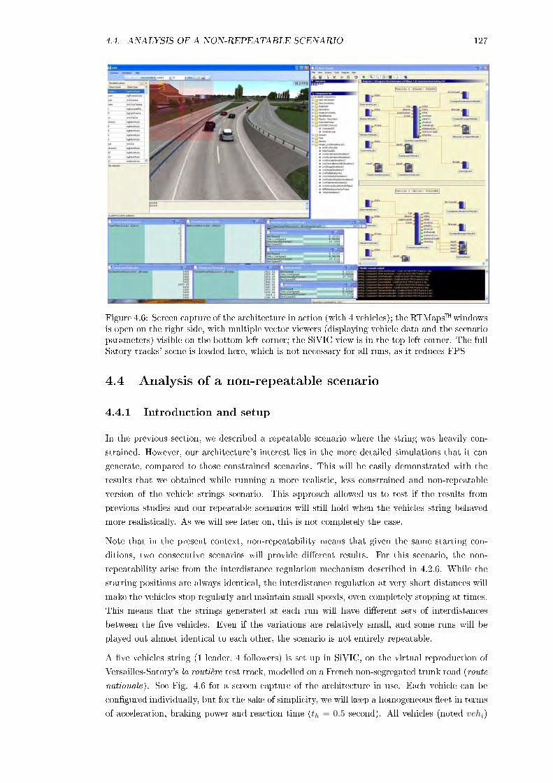
4.4. ANALYSIS OF A NON-REPEATABLE SCENARIO 127

Figure 4.6: Screen capture of the architecture in action (with 4 vehicles); the RTMaps windowsis open on the right side, with multiple vector viewers (displaying vehicle data and the scenarioparameters) visible on the bottom left corner; the SiVIC view is in the top left corner. The fullSatory tracks' scene is loaded here, which is not necessary for all runs, as it reduces FPS

4.4 Analysis of a non-repeatable scenario

4.4.1 Introduction and setup

In the previous section, we described a repeatable scenario where the string was heavily con-

strained. However, our architecture's interest lies in the more detailed simulations that it can

generate, compared to those constrained scenarios. This will be easily demonstrated with the

results that we obtained while running a more realistic, less constrained and non-repeatable

version of the vehicle strings scenario. This approach allowed us to test if the results from

previous studies and our repeatable scenarios will still hold when the vehicles string behaved

more realistically. As we will see later on, this is not completely the case.

Note that in the present context, non-repeatability means that given the same starting con-

ditions, two consecutive scenarios will provide dierent results. For this scenario, the non-

repeatability arise from the interdistance regulation mechanism described in 4.2.6. While the

starting positions are always identical, the interdistance regulation at very short distances will

make the vehicles stop regularly and maintain small speeds, even completely stopping at times.

This means that the strings generated at each run will have dierent sets of interdistances

between the ve vehicles. Even if the variations are relatively small, and some runs will be

played out almost identical to each other, the scenario is not entirely repeatable.

A ve vehicles string (1 leader, 4 followers) is set up in SiVIC, on the virtual reproduction of

Versailles-Satory's la routière test track, modelled on a French non-segregated trunk road (route

nationale). See Fig. 4.6 for a screen capture of the architecture in use. Each vehicle can be

congured individually, but for the sake of simplicity, we will keep a homogeneous eet in terms

of acceleration, braking power and reaction time (th = 0.5 second). All vehicles (noted vehi)

128 CHAPTER 4. SIMULATION ARCHITECTURE FOR CS APPLICATIONS

have tinter = 2.5 seconds; except veh2 for which tinter = 1.5 seconds, in order to simulate a

slightly more risky driving. Having only a single aggressive driver can be seen as a conservative

gure. Indeed, according to government statistics, more than half (56.4%) of the drivers do

not follow safe interdistances recommendations (at least 2 seconds) in dense trac [3]. For this

scenario, vehicles are also operating in reactive mode, maintaining enough similarity with the

previous studies we aim at reproducing.

Contrary to the previous repeatable scenario, the vehicles start and stopped while grouped to-

gether in one location on the track. From this starting position, the vehicles arrange themselves

in a string on the right-hand lane, and progressively speed up to 70 km/h generating, as we

mentioned, a dierent string each time. Follower vehicles are equipped with receptors, depend-

ing on the desired equipment ratio. IVC equipment is randomly selected for each individual

follower (initially it was planned in pre-processing, but the architecture's latest version allows

to do it directly online) until there is the required number of equipped vehicles. The equipment

is reset with each new run. The emergency braking event takes place in a long straight section

approximately 700 metres from the starting position.

The scenario was replayed at least a hundred times for each of the following equipment ratios:

0/5, 2/5, 3/5, 4/5, and 5/5. The ρ = 1/5 case is not simulated as it corresponds to having only the

leader vehicle equipped, which is no dierent from ρ = 0/5 in this scenario. A total of 716 runs

were simulated, which generated 1,197 crashes. The following variables were recorded for all

vehicles: curvilinear abscissa, TTC, dtarget, V , Vref , emergency frame broadcast and instances

of collisions.

4.4.2 Crash number analysis

Fig. 5.18 shows the normalised total rear-end crashes at dierent equipment ratios. Crash

numbers have been normalised to compensate for the dierent number of runs at each value of

ρ; the number of crashes recorded for ρ = 0/5 is set as the reference and valued at 100, allowing

an immediate percentage comparison with other values of ρ. By introducing 2 IVC-equipped

vehicles (ρ = 2/5, or 40%), the number of crashes fell by 17%; with ρ = 3/5, the number of

crashes fell by 50%, and with ρ = 4/5, the number fell by 80%. In a completely equipped string,

no crashes were recorded. Note that the crash number is maintained at 100 for ρ = 1/5 since,

as we explained in the previous subsection, it is indistinguishable from ρ = 0/5.

As we already stated, in [22, 23] the number of vehicles in the string was signicantly higher,

which allowed for better granularity of ρ. Compared to the repeatable scenario however, the

large number of simulation runs make it possible to obtain more rened and more realistic

results. Contrary to [23], our results do not show a strong 1x type decrease in crashes when the

IVC equipment ratio increases. However, they follow the same trend; for example at a 2,600

vehicles/hour capacity, the reduction in crash numbers between ρ = 0% to ρ = 80% is very

similar to our results. Furthermore, it can be noted that in our scenario, IVC equipment starts

to provide a reasonable safety increase with only more than 50% of equipped vehicles. This is

probably an issue related to the limited granularity aorded by 5 vehicles strings. Nonetheless,

our results are coherent with the EEBL scenario and shows that our CS simulation architecture

can be used to complement larger simulations like [23] by oering more detailed results, which

we shall look into from now on.

Being able to record and study variability inside the string for each individual vehicle is a major

improvement in our architecture design. Dierent kinds of data can be considered for study,

4.4. ANALYSIS OF A NON-REPEATABLE SCENARIO 129

0 10 20 30 40 50 60 70 80 90 1000

20

40

60

80

100

Percentage of IVC−equipped vehicles

Cra

shes

Total number of crashes(with non equipped scenario as 100 basis)

0 10 20 30 40 50 60 70 80 90 1000

1

2

3

Percentage of IVC−equipped vehicles

Cra

shes

Average number of crashes per run(a) Normalised crashes count for the whole string

0 10 20 30 40 50 60 70 80 90 1000

50

100

150

Percentage of IVC−equipped vehicles

Cra

shes

Total number of crashes (with non equipped scenario as 100 basis)

Vehicle 2Vehicle 3Vehicle 4Vehicle 5Whole string

(b) Normalised crashes count for the whole string and each individual vehicles

Figure 4.7: Illustrations of the reduction in crashes obtained by introducing IVC in the vehiclesstring

130 CHAPTER 4. SIMULATION ARCHITECTURE FOR CS APPLICATIONS

which we will demonstrate using two examples. Firstly, it is possible to extract information on

the behaviour of each vehicle concerning crash patterns associated with them over the whole

experimental run and secondly, their behaviour during a single run.

4.4.3 Crashes number pattern for individual vehicles

In a detailed analysis of our rst example, Fig. 4.7b reproduces Fig. 5.18 data (the dashed

black curve), and overlays it with the normalised crash counts for each individual vehicle. From

this gure, it is evident that while the string taken globally see less crashes with increased

IVC equipment, it is not necessarily the case with individual vehicles. Indeed, for veh4, having

40% of IVC equipment led to a 47% increase in the number of crashes encountered by this

vehicle. At 60% equipment (ρ = 3/5), the crash count was still 15% higher than in a fully

non-equipped scenario. At 80% equipment, the percentage decrease in crashes encountered by

veh4 was similar to the other vehicles with 40% equipment.

At face value, this result would suggest that while drivers would collectively benet from using

EEBL, some drivers would see the likelihood of them crashing increase. Obviously, this is an

unacceptable conclusion in the name of road safety. This is further aggravated by the knowledge

that, if the absolute number of crashes is considered, veh4 is the one with the least number of

crashes at ρ = 0/5. How could introducing IVC make the previously safest vehicle, the least

safe? We shall investigate the reasons for this phenomenon, which will demonstrate it is not

something possible in an actual on road situation.

Indeed, from the detailed recordings, veh4 appears to be following veh3 with a slightly above

average interdistance. In the scenario without IVC, this is not an issue and the vehicle manages

to stop before colliding with veh3 in most cases, hence it has a lower number of crashes relative

to the others. On the other hand, at ρ = 2/5, if veh2 or veh3 are equipped with IVC, veh3 will

have a tendency to stop earlier than it did in the non-equipped scenario. Because of this, the

relative speed between the two vehicles is large when veh4's controller starts to press the brakes.

In that case, even at maximum braking capability, veh4 is unlikely to stop before colliding with

veh3, which led to the 50% increase in crashes we measured.

Unfortunately, this behaviour stands out as a limitation to our simulation. Indeed, on a real road

situation, veh4's driver would become aware of veh3's braking manoeuvre with the activation

of its braking lights so, veh4 would thus stop much earlier than what the current controller

decides to do. Thus, our scenario articially increases the chances of a crash for that specic

vehicle. Future work shall allow simulating this type of behaviour more appropriately.

Nonetheless, this happens only with veh4, which does not misrepresent the results for the whole

string. All the remaining vehicles behaved according to the scenario expectations. Additionally,

if we lter the runs to keep only the ones where veh4's interdistance is comparable to the string's

average, veh4 behaves just like the other vehicles. Also note that veh2's count is higher than

the others on average (ignoring veh4) because of its aggressive driving style, which is consistent

with the scenario settings.

4.4.4 Behaviour of individual vehicles

For this second example, we focus on one vehicle in a single run. Fig. 4.8 shows the variables

related to the interdistance regulation for veh3, taken during a ρ = 3/5 run, where it was not

4.4. ANALYSIS OF A NON-REPEATABLE SCENARIO 131

5.65 5.7 5.75 5.8 5.85 5.9 5.95 6 6.05 6.1

x 108

0

5

10

15

20

Time (microseconds)

Sp

eed

(m

etre

s/se

con

ds)

5.65 5.7 5.75 5.8 5.85 5.9 5.95 6 6.05 6.1

x 108

0

20

40

60

Dis

tan

ce t

o le

adin

g v

ehic

le (

met

res)

Distance to leading vehicle

SpeedVrefCrash detection

Figure 4.8: Detailed variables measurements for one vehicle during a simulation run

equipped with an IVC device. The command Vref represented by the blue curve (left-hand

axis) depends on either transponder-distributed speed instructions, which is the case when it is

limited to 5 metres/second for a few seconds at the beginning of the run, or on dtarget, shown by

the green dotted curve (right-hand axis), via equation 4.4. Two types of interdistance variations

are visible on the gure: (1) normal variations triggered when the leading vehicle is actually

getting closer to veh3, such as is the case around the 5.85× 108 or 5.9× 108 timestamps; and

(2) sharp variations that occurs when either veh2 or veh3 is turning and thus veh2 exits the

frontal laserscanner's narrow beam, this happen a lot between the 5.75 × 108 and 5.85 × 108

timestamps. The interdistance measurement is capped at 50 metres, the useful range of the

laserscanner model used for this scenario.

V (red curve, left-hand axis) is well regulated according to Vref . On three occasions the vehicles

came close enough for veh3's controller to compute that it was necessary to press the brakes.

This usually happens due to the propagation of braking waves started by vehicles at turns

or when they enter or exit dierent speed regulation zones. One can also note, just after

the 5.7 × 108 timestamp, a brief period for which Vref uctuates a lot, very quickly. This

is a visual representation of the interdistance regulation behaviour that led to the scenario's

non-repeatability.

Eventually, the vehicle's emergency braking pattern can be analysed from these data. Around

the 6.05×108 timestamp, the vehicle starts to stop because dtarget becomes too small; the delay

introduced by the human reaction time is clearly visible: when the vehicle starts to brake, the

interdistance has already shrunk by more than 10 metres. Even at maximum braking power,

veh3 cannot stop before the impact with the preceding vehicle, which is shown by the vertical

black dotted line just after the 6.1×108 timestamp. The impact takes place at a relatively slow

speed of 6 metres.seconds-1(~22 km/h).

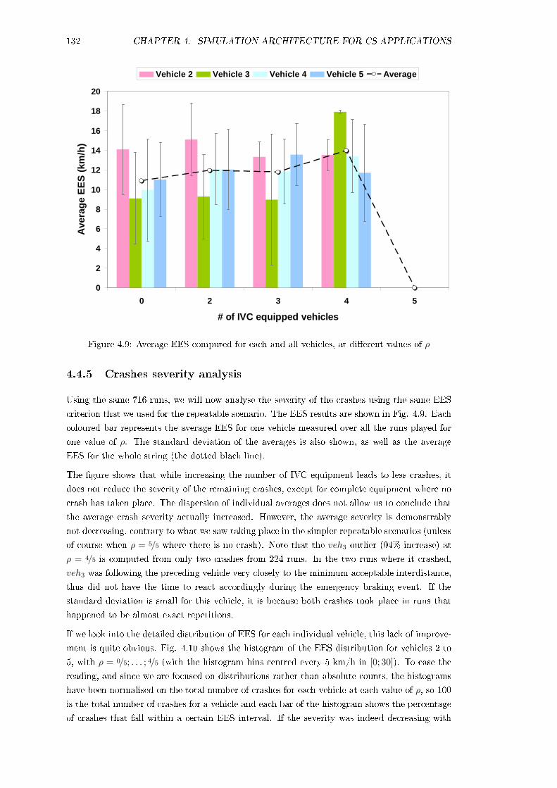
132 CHAPTER 4. SIMULATION ARCHITECTURE FOR CS APPLICATIONS

0

2

4

6

8

10

12

14

16

18

20

0 2 3 4 5

# of IVC equipped vehicles

Ave

rag

e E

ES

(km

/h)

Vehicle 2 Vehicle 3 Vehicle 4 Vehicle 5 Average

Figure 4.9: Average EES computed for each and all vehicles, at dierent values of ρ

4.4.5 Crashes severity analysis

Using the same 716 runs, we will now analyse the severity of the crashes using the same EES

criterion that we used for the repeatable scenario. The EES results are shown in Fig. 4.9. Each

coloured bar represents the average EES for one vehicle measured over all the runs played for

one value of ρ. The standard deviation of the averages is also shown, as well as the average

EES for the whole string (the dotted black line).

The gure shows that while increasing the number of IVC equipment leads to less crashes, it

does not reduce the severity of the remaining crashes, except for complete equipment where no

crash has taken place. The dispersion of individual averages does not allow us to conclude that

the average crash severity actually increased. However, the average severity is demonstrably

not decreasing, contrary to what we saw taking place in the simpler repeatable scenarios (unless

of course when ρ = 5/5 where there is no crash). Note that the veh3 outlier (94% increase) at

ρ = 4/5 is computed from only two crashes from 224 runs. In the two runs where it crashed,

veh3 was following the preceding vehicle very closely to the minimum acceptable interdistance,

thus did not have the time to react accordingly during the emergency braking event. If the

standard deviation is small for this vehicle, it is because both crashes took place in runs that

happened to be almost exact repetitions.

If we look into the detailed distribution of EES for each individual vehicle, this lack of improve-

ment is quite obvious. Fig. 4.10 shows the histogram of the EES distribution for vehicles 2 to

5, with ρ = 0/5; . . . ; 4/5 (with the histogram bins centred every 5 km/h in [0; 30]). To ease the

reading, and since we are focused on distributions rather than absolute counts, the histograms

have been normalised on the total number of crashes for each vehicle at each value of ρ, so 100

is the total number of crashes for a vehicle and each bar of the histogram shows the percentage

of crashes that fall within a certain EES interval. If the severity was indeed decreasing with

4.4. ANALYSIS OF A NON-REPEATABLE SCENARIO 133

1 2 3 4 5 60

20

40

60

80

100

EES (km/h)

Per

cen

tag

e

Vehicle 2

1 2 3 4 5 60

20

40

60

80

100

EES (km/h)

Per

cen

tag

e

Vehicle 3

1 2 3 4 5 60

20

40

60

80

100

EES (km/h)

Per

cen

tag

e

Vehicle 4

1 2 3 4 5 60

20

40

60

80

100

EES (km/h)

Per

cen

tag

e

Vehicle 5

0/52/53/54/5

Figure 4.10: Distribution of EES for each vehicles, at ρ = 0/5; . . . ; 4/5

an increase in ρ, we would expect the distributions to slide towards the left, i.e. towards lower

EES. However, there is no such general movement. The shapes of the distribution uctuate,

but the averages remain relatively stable or can even increase in some cases.

While the EES absolute values remain largely under any dangerous threshold due to the scenario

conditions, implications are worrying at higher speeds. Indeed, from the point of view of a

system's contribution to road safety, it is better to have several weak crashes, where no one is

injured, then one or two violent ones, where fatalities occur. In [22], it was shown that using the

raw number of crashes to evaluate IVC's contribution to the string's safety was always more

pessimistic than using an EES-based severity criterion. However, we found here that while

the number of crashes indeed decreased signicantly, the severity of the remaining crashes did

not decrease. In this case, a crash number-based criterion would have been considerably more

optimistic than the EES-based severity criterion.

134 CHAPTER 4. SIMULATION ARCHITECTURE FOR CS APPLICATIONS

4.5 Conclusion

In this chapter, our goal was to design a framework that could be used to support research on

the limitations of Cooperative Systems (CS) in general, and augmented perception in particular.

In Chapter 2 we concluded it was better to focus on using more realistic simulations instead

of focusing on real-world systems. Developing and prototyping CS applications within a

simulated environment comes with stringent requirements. The simulation has to integrate

with models of the road environment, vehicles, sensors and communication technologies which

are all consistent with the law of physics. Using simulation to meet these requirements enables

a much wider eld of research and experimentation than keeping a focus on actual on-road

systems, as the logistical and experimental protocol constraints are lifted.

We have found that there is a need for improved realism in terms of CS simulation. In order

to answer this, we developed a cooperative system simulation architecture within the SiVIC-

RTMaps interconnected platforms. This architecture uses the SiVIC-RTMaps' capabilities

to provide realistic simulations that meets the aforementioned requirements, while allowing

some exibility in terms of what can be developed within it. It improves upon previous sim-

ulation architectures developed at LIVIC (as seen in Gruyer et al. [97], Vanholme et al. [98]

for a co-pilot simulation using a simple I2V mechanism, or in Mourllion [31] for a high level

augmented perception simulation); the two main improvements concern; (1) the introduction of

the empirical modelisation of 802.11p IVC discussed in Chapter 3; and (2) an improved vehicle

controller, allowing for an automated vehicle to behave more like a human-driven one. The ne

granularity of the physical models, and the number of accessible variables within the simulation,

allows studying the behaviour of an individual vehicle over the length of an entire scenario. We

validated this architecture by reproducing results from previous research on the contribution of

IVC to the reduction of rear-end crashes in vehicle strings with a heavily-constrained repeat-

able scenario. Our results are coherent with previous studies both in terms of the reduction of

crash numbers and reduction in the severity of the crashes (which is computed with the EES

criterion).

However, at the end of Chapter 3, it was concluded that 802.11p performance has been over-

estimated by previous research. This begged the question, could this mean that the safety

benets of CS have been overestimated too, by a form of assumptions propagation? In order

to provide a preliminary answer to this question, as far as EEBL is concerned, we implemented a

more realistic, non-repeatable scenario that allowed analysing crashes and vehicle behaviour in

the string with considerable detail. Our results conrmed IVC's eciency to reduce collisions,

showing that IVC limitations are not a problem within this scenario. However, we also obtained

surprising and potentially worrying results regarding the severity of the crashes. Indeed, we

found that contrary to expectations, the average severity of a crash appears to remain constant

when an IVC is introduced in the string. Earlier results [22, 31, 23] suggested that introducing

IVC would lead to less crashes, and that the remaining crashes would be less severe. Our results

suggest that, indeed there will be less crashes however, on average the remaining crashes will

remain as severe as previously. This implies that if the material cost of a series of crashes in a

vehicles string would decrease (less damaged vehicles), the human cost might actually increase

in some cases.

As this scenario is a representative of a form of CS application that will be proposed to main-

stream users in a not too distant future (which was a reason we selected this as our reference

scenario), these results are not trivial and further consideration should be given to them before

4.5. CONCLUSION 135

deploying an actual EEBL application. This study allowed us to demonstrate the interest of our

architecture outside of the context of augmented perception, into a more general CS context.

From now on, our architecture will provide the environment within which augmented perception

will be built and evaluated.

Summary of chapter's contributions

Outcomes

A generalist Cooperative Systems simulation architecture/framework was developed.

Key ndings

When improving the realism of the simulation, an EEBL system appears to not

improve the average severity of a crash in a vehicles string, contrary to previous

results.

However, the safety benets of EEBL according to the number of crashes criterion

were conrmed.

Limitations

Controllers of the vehicles generate behaviours under certain conditions that might

not be the best representation of real behaviours.

136 CHAPTER 4. SIMULATION ARCHITECTURE FOR CS APPLICATIONS

Chapter 5

Building an augmented map

5.1 Introduction

In the previous chapter, we designed a simulation architecture aimed at supporting studies on

higher-level Cooperative Systems (CS) applications, such as ones that looked into the safety

benets of these systems. We argued that if oered signicant improvements over previous

simulations of CS applications, notably by including the empirical performance model of 802.11p

IVC that we developed in Chapter 3. The architecture's capabilities were demonstrated by

studying an EEBL application, which allowed us to obtain new results regarding the safety

benets of EEBL. We found that contrary to expectations, the average crash severity appeared

to be unaected by the EEBL application. Our results suggest that there will be less crashes,

leading to a probable decrease in material costs, but that the human cost will remain stable,

or might actually increase in some rare cases. Eventually, the CS simulation architecture was

also poised to become the core framework in which further research on augmented perception

would take place.

The rst aim of this chapter is to design an augmented map building architecture, within the

simulation framework that was presented in the previous chapter. Similar to the simulation

framework that supports it, this map-building architecture should be generalist, and be able to

accommodate the exchange of both localisation, proprioceptive and exteroceptive data.

The second aim of this chapter is to evaluate the performance of augmented perception for risk

assessment by comparing it to non-cooperative perception within the context of a specied CS

safety-orientated application. Logically, we will use the vehicles string reference scenario. This

study will provide answers to the following principal research questions:

1. What are augmented perception's limitations, given current technology in embedded com-

puting and telecommunications?

2. Can an augmented map-based risk assessment system be more ecient than a similar

non-cooperative system?

Our rst step is to build the generalist augmented map building architecture. Having a general-

ist approach implies that (1) we dissociate the augmented map from its client applications, and

that (2) the architecture should be able to accommodate dierent construction approaches, such

138 CHAPTER 5. BUILDING AN AUGMENTED MAP

as decentralised or server-based fusion. The rst point means creating an augmented map that

has features which can be used by dierent types of client applications. The second point can

be achieved through an adequate re-arrangement of the components dedicated to constructing

the augmented map within the CS simulation architecture, by forming distinct fusion trees. A

centralised server-like approach can be simulated by having a single map-building tree receiving

data from all vehicles, while a decentralised approach can be simulated with having as many

map-building trees as vehicles in the simulation. As part of this design, we have ensured that

the exchange of complex local maps is covered. Indeed, within the context of augmented per-

ception, the exchange of local maps including exteroceptive data is still fairly recent. Current

augmented perception systems are mostly classied to two types: (1) systems that exclusively

use localisation and proprioceptive local and remote data; and (2) systems that use the same

remote data and complement them with local exteroceptive data.

On the other hand, the data fusion algorithms and methods are xed within the architecture's

components. Data fusion is performed using Kalman ltering and the Dempster-Shafer Theory,

as a follow-up to previous works concerning the adaptation of these mathematical principles to

augmented perception. Theoretical considerations will be presented in further detail before the

actual design of the architecture.

After the map-building architecture has been designed, we test it on our reference scenario

with a risk-assessment system. The risk of the current driving situation is computed for each

vehicle, from information received through local perception or augmented perception. This

latter approach accounts for the limitations of IVC performance that we studied in the previous

chapters, and allows obtaining results which are close to what could be expected to happen on

the road. We show that the augmented map-based risk assessment process allows for up to

7 seconds of additional advance warning compared to a non-cooperative process, despite the

presence of IVC imperfections. This demonstrates the usefulness of augmented perception in

the reduction of road fatalities.

Chapter Outline

The rst section consists of a literature review on augmented perception, including a few remain-

ders on data fusion. It helps understanding the current division in two schools regarding the

granularity of exchanged information, and details issues with spatio-temporal synchronisation

and data independence.

The second section provides details on the theoretical foundations for our map-building archi-

tecture , including Kalman ltering, the Dempster-Shafer Theory and our approach to multi-

hypothesis tracking. Afterwards, the third section exposes the design of the map-building

architecture within the framework laid out in Chapter 4.

The fth section provides the performance evaluation of the augmented map-building architec-

ture, comparing it with non-cooperative perception for a specic risk-assessment problem.

Eventually, the sixth section concludes this chapter by summarising its outcomes .

5.2. GENERAL PRINCIPLES AND LITERATURE REVIEW 139

5.2 General principles and Literature review

5.2.1 Multi-sensors fusion

5.2.1.1 Introduction

Multi-sensors fusion is a classic way to build the local map. A local map is a representation

of the outside environment surrounding a vehicle, as perceived by the vehicle's sensors. The

part of the environment that is perceived or observed by the sensors is usually called the scene.

Embedded sensors collect information about the environment, but the type and quality of such

information often diverge. Actually, each individual sensor creates its own representation of

the environment. Then, these separate representations can be combined through multi-sensors

fusion to create a unied multi-sources representation.

Building such a local map is done by joining tracks representing objects in the vehicle's en-

vironment together into a common representation and fusing tracks describing the same real

objects. The goal of this process is to improve the accuracy, reliability and robustness of the

perception, so that errors in some sensors or processing algorithm will not make the perceived

scene completely irrelevant. Representing one's environment is achieved through a number

of stages, which are usually considered as a sequence following two major axes: (1) detec-

tiontrackingclassication on one hand, and (2) mappinglocalisation on the other hand [103].

Fig. 5.1 shows the relationship between these stages.

Detection: also called the segmentation stage, it consists of identifying which measure-

ments originate from the same real object, among the raw data. Thus, this stage outputs

a list of objects located into the scene. No hypothesis on the object's nature is taken at

this stage.

Tracking: it consists of following the timely evolution of detected objects and estimating

a number of objects' properties. For example tracking one object during several sensors

timestamps can allow estimating its past motion and predicting its future motion: speed,

heading, etc. To achieve this, tracking covers two sub-stages - association and fusion.

Association consists of linking together objects detected at time ti with objects detected

at time ti−1. Fusion then combines these two objects into a single object. Tracked objects

are usually called tracks.

Classication: it consists of completing the detection stage by identifying the nature of

the detected object. This stage is essentially orientated towards higher level applications

or interest zone extraction.

Mapping: it consists of reconstructing an object's outline. Indeed, it is probable that

at time ti a detected object is partially occluded by another object. Its exact shape, its

outline, is thus not visible. Mapping allows reconstructing the object's outline over several

timestamps, so this data can be sent to higher-level applications. A good mapping can

also be useful to the classication stage.

Localisation: this stage tries locating a vehicle in its environment according to raw sensors

data. Excluding satellite positioning systems that provide an absolute localisation data

as their raw output, localisation here implies localisation approaches relative to objects

within the scene.

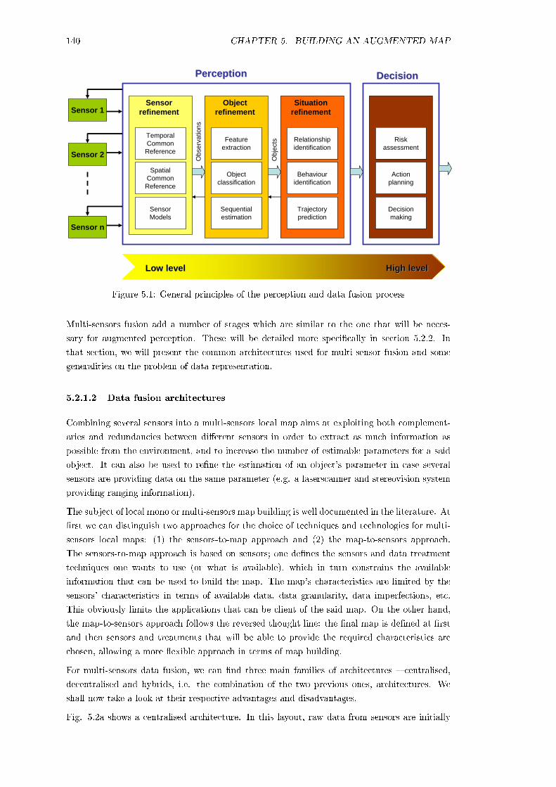
140 CHAPTER 5. BUILDING AN AUGMENTED MAP

Sensor 1

TemporalCommonReference

SpatialCommonReference

SensorModels

Featureextraction

Objectclassification

Sequentialestimation

Relationshipidentification

Behaviouridentification

Trajectoryprediction

Sensor 2

Sensor n

Riskassessment

Actionplanning

Decisionmaking

Sensorrefinement

Objectrefinement

Situationrefinement

PerceptionPerception DecisionDecision

LowLow levellevel High High levellevel

Obs

erva

tions

Obj

ects

Figure 5.1: General principles of the perception and data fusion process

Multi-sensors fusion add a number of stages which are similar to the one that will be neces-

sary for augmented perception. These will be detailed more specically in section 5.2.2. In

that section, we will present the common architectures used for multi-sensor fusion and some

generalities on the problem of data representation.

5.2.1.2 Data fusion architectures

Combining several sensors into a multi-sensors local map aims at exploiting both complement-

aries and redundancies between dierent sensors in order to extract as much information as

possible from the environment, and to increase the number of estimable parameters for a said

object. It can also be used to rene the estimation of an object's parameter in case several

sensors are providing data on the same parameter (e.g. a laserscanner and stereovision system

providing ranging information).

The subject of local mono or multi-sensors map building is well documented in the literature. At

rst we can distinguish two approaches for the choice of techniques and technologies for multi-

sensors local maps: (1) the sensors-to-map approach and (2) the map-to-sensors approach.

The sensors-to-map approach is based on sensors; one denes the sensors and data treatment

techniques one wants to use (or what is available), which in turn constrains the available

information that can be used to build the map. The map's characteristics are limited by the

sensors' characteristics in terms of available data, data granularity, data imperfections, etc.

This obviously limits the applications that can be client of the said map. On the other hand,

the map-to-sensors approach follows the reversed thought line: the nal map is dened at rst

and then sensors and treatments that will be able to provide the required characteristics are

chosen, allowing a more exible approach in terms of map building.

For multi-sensors data fusion, we can nd three main families of architectures centralised,

decentralised and hybrids, i.e. the combination of the two previous ones, architectures. We

shall now take a look at their respective advantages and disadvantages.

Fig. 5.2a shows a centralised architecture. In this layout, raw data from sensors are initially

5.2. GENERAL PRINCIPLES AND LITERATURE REVIEW 141

Sen

sor

1

Sen

sor

2

Sen

sor

n

Mu

lti-

sen

sors

det

ecti

on

, tra

ckin

g,

clas

sifi

cati

on

, lo

calis

atio

n &

map

pin

gS

ynch

ron

isat

ion

Lo

cal

Lo

cal

map

map

(a)Genericcentralisedarchitecture

Sen

sor

1

Sen

sor

2

Sen

sor

n

Mu

lti-

sen

sors

asso

ciat

ion

an

d f

usi

on

Syn

chro

nis

atio

nL

oca

l L

oca

l m

apm

apL

oca

l det

ecti

on

,tr

acki

ng

, cla

ssif

icat

ion

,m

app

ing

& lo

calis

atio

n

Lo

cal d

etec

tio

n,

trac

kin

g, c

lass

ific

atio

n,

map

pin

g&

loca

lisat

ion

Lo

cal d

etec

tio

n,

trac

kin

g, c

lass

ific

atio

n,

map

pin

g&

loca

lisat

ion

(b)Genericdecentralised

architecture

Las

er s

can

ner

Ste

reo

visi

on

Filt

erin

g(o

bje

cts

det

ecti

on

)

Filt

erin

g(o

bje

cts

det

ecti

on

)

Mu

lti-

ob

ject

s&

mu

lti-

trac

ksas

soci

atio

n

Mu

lti-

ob

ject

s&

mu

lti-

trac

ksas

soci

atio

n

Tra

ckin

g(K

alm

an f

ilter

)

Tra

ckin

g(K

alm

an f

ilter

)

Mu

lti-

trac

ksas

soci

atio

n a

nd

fu

sio

nM

apM

ap

(c)Exampleof

decentralised

approach

Sen

sor

1

Sen

sor

2

Sen

sor

i

Mu

lti-

sen

sors

det

ecti

on

, tr

acki

ng

, cla

ssif

icat

ion

,lo

calis

atio

n &

map

pin

gS

ynch

ron

isat

ion

Sen

sor

n-2

Sen

sor

n-1

Sen

sor

n

Mu

lti-

sen

sors

asso

ciat

ion

an

d f

usi

on

Syn

chro

nis

atio

nL

oca

l L

oca

l m

apm

ap

Lo

cal d

etec

tio

n,

trac

kin

g, c

lass

ific

atio

n,

map

pin

g&

loca

lisat

ion

Lo

cal d

etec

tio

n,

trac

kin

g, c

lass

ific

atio

n,

map

pin

g&

loca

lisat

ion

Lo

cal d

etec

tio

n,

trac

kin

g, c

lass

ific

atio

n,

map

pin

g&

loca

lisat

ion

(d)Generichybridarchitecture

Figure

5.2:Data

fusionarchitectures

142 CHAPTER 5. BUILDING AN AUGMENTED MAP

Stereo

vision

Filterin

g(o

bjects

detectio

n)

Map

Map

Laser scan

ner

Filterin

g(o

bjects

detectio

n)

Mu

lti-ob

jects&

mu

lti-tracksasso

ciation

Trackin

g(K

alman

filter)

Mu

lti-tracksasso

ciation

and

fusio

n

(a)Anexam

pleof

hybrid

approach

Rad

ar

Infrared

senso

rs

Laser scan

ner

IFF

(radio

)

Electro

nic

warfare

senso

rs

Detectio

n, trackin

gclassificatio

n

Detectio

n, trackin

gclassificatio

n

Detectio

n, trackin

gclassificatio

n

Detectio

n, trackin

gclassificatio

n

Detectio

n, trackin

gclassificatio

n

Mu

lti-senso

rsasso

ciation

Mu

lti-ob

jectsasso

ciation

and

fusio

nM

apM

ap

(b)Anoth

erexam

pleof

hybrid

approach

Figure

5.3:Data

fusio

narch

itectures

(contin

ued)

5.2. GENERAL PRINCIPLES AND LITERATURE REVIEW 143

synchronised, if necessary, before any treatments are applied to them. There is few or no

treatment directly at the sensor level, the treatment as a whole is made later, at a higher

level. In this architecture one does not have proper multi-sensors association, tracking and

fusion, as all the data are used at the same time to extract objects and track them; the process

is conducted directly on the raw data ow of several sensors at the same time. Historically,

centralised approaches have been the rst type of multi-sensors fusion to be developed [104].

The main advantage of centralised architectures lies in their good tracking performance [105].

However they can, in modern settings, be overloaded by computation load in complex envir-

onments with numerous sensors and staunch real-time requirements (which is the case on the

road). Furthermore in such centralised architectures, the error is global to the whole system

and strongly inuenced by the least performing sensors. A single sensor's defect will also aect

the whole system. One can nd generic examples of centralised example in [106] (an automated

electronic components recognition system) or in [107] (data fusion between laser scanner, inertial

data, digital maps and propagated data), inter alia.

Fig. 5.2b shows the principles of a decentralised architecture. Raw sensors data are at rst

treated in order to extract objects, then these objects are synchronised, if necessary, and sent

to an association-fusion process that creates the local map. Decentralised architectures are also

sometimes called hierarchical [104] or autonomous architectures [108]. Decentralised architec-

tures have the following advantages: treatments can be adapted to each sensor according to their

nature and performances, the global computing load is reduced, and the system's robustness to

a sensor's defect or breakdown is increased.

A potential disadvantage of decentralised approaches is that the necessary independence of data

might be compromised [104, 105] (for more on this problem, refer to section 5.12). Salahshoor

et al. [105] also noted that decentralised architectures are conceptually more complex than

centralised architectures, which may limit their scope. One example (shown on Fig. 5.2c)

is presented by Labayrade et al. [109] for a multi-sensors obstacle detection system using a

laserscanner and stereovision. However, the authors note that stereovision is very inaccurate

beyond a range of about 15 metres, which renders the treatment of stereovision data dicult.

They solve this problem using the next kind of architecture we will describe (see Fig. 5.3a).

Eventually, Fig. 5.2d shows a hybrid architecture. It combines the centralised and decentral-

ised approaches with the aim of beneting from advantages on both sides. Fig. 5.2d diagram

is far from exhaustive, it is possible to design other forms of this architecture, more complex

or with dierent levels of centralisation and decentralisation. The main advantage of hybrid

architectures is that they allow ne-tuning the map-building system according to users' require-

ments as well as according to the sensors characteristics. One can for example locally treat the

data of the most precise sensors through a separated branch from the main central branch in

a partially decentralised architecture to minimise the impact of the least precise or reliable

sensors. A hybrid architecture also allows solving specic issues of the other architectures while

generally beneting from their combined advantages. For example as we already mentioned in

[109] stereovision is inaccurate beyond 15 metres, which limits the interest of performing a full

tracking processing on this data. A hybrid architecture shown in Fig. 5.3a was proposed in

order to avoid this problem by performing a full processing on laserscanner data and only using

stereovision-extracted objects to increase the condence on the laserscanner tracks, without any

tracking of these stereovision objects. Another example can be found in Gad and Farooq [110]:

the author selected a hybrid architecture, shown in Fig. 5.3b, which was deemed more ecient

144 CHAPTER 5. BUILDING AN AUGMENTED MAP

than solely centralised or decentralised architecture for the problem of military maritime tac-

tical surveillance. This architecture's interest is that the same sensors data are processed in

two dierent branches before being united. The main disadvantage of hybrid architectures also

lies in their conceptual complexity, similarly to decentralised architectures.

5.2.1.3 Format and data representation

As we mentioned, the local map is modulated according to the sensors' capabilities and the

applications that will use it. An adequate way to represent all the accessible information or, at

least, a part of it must be selected. It would be unwise to try to represent all the parameters

estimated for one object, while a specic application might only be interested in a specic

subset of information about an object. This problem is also relevant to augmented perception,

notably given the fact that we aim at having a generic-enough augmented map that can be used

to feed dierent client applications. The following data representation formats can be found in

the literature - direct, attributes, grid and Gaussian representations.

A direct representation, as its name suggests, directly represents raw sensors data. This kind

of representation is preferred if one has accurate enough sensors, such as laser scanners for

example. Direct representations allow for a good precision of some objects' parameters (shape,

position) but, as there is no preliminary treatment whatsoever on the data, they cannot be

used to represent estimated or predicted objects. It means direct representations are limited to

directly measured data only, for visualisation or pre-treatment purposes. Because of that, they

are said to be geometric-only representation. Note that direct representations might suer

from memory problems if the sensor(s) sampling frequency is high. Also, they do not model

imperfections. Fig. 5.4 shows an example of such direct representations.

Attributes representations uses objects which are composed of so-called state vectors to repres-

ent the known objects in the scene. They usually limit the range of the available parameters to

some which are chosen according to what will be the map's nal use. For example a vehicle-like

object could be represented by a state vector containing its GPS-measured absolute position,

speed, heading and dimensions; a tree could be represented by a vector containing solely the

equivalent rectangle occupied by the tree in a at two dimensional representation. Imperfec-

tions are included in attributes-based representation but usually not with the most realistic

modelling. The advantage of these representations is essentially its memory eciency and that

it can include treatments' outputs (tracking, etc.). As they require more parameters to obtain

a sucient description of objects, attributes representations might be disadvantaged when used

in heterogeneous environments. Fig. 5.5 (from Gate [103]) show an example of an attributes

representation compared to the real environment it represents. This is the standard type of

data representation that is used within the context of the present thesis.

A grid representation divides space into a grid where resolution might be xed or variable.

Each grid element, or cell, is associated with a unique probabilistic parameter; this parameter

will usually be the probability that the cell is occupied by an object of any nature. We can

nd an example in [42] for local laserscanner data. Grid representations are good at modelling

precisely all the imperfections on the cell's parameter; however, they have important memory

and computational requirements, in order to maintain a sucient grid resolution. For safety

application, grid resolutions in the centimetre range are required.

Gaussian representations can be found in two categories: (1) methods that stem from direct

representations and try to solve their imperfection's modelling issues; and (2) methods that stem

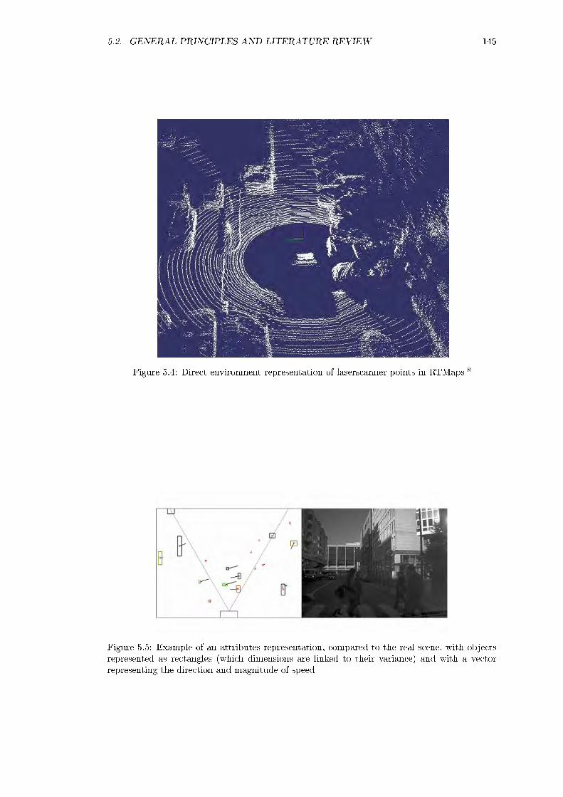
5.2. GENERAL PRINCIPLES AND LITERATURE REVIEW 145

Figure 5.4: Direct environment representation of laserscanner points in RTMaps

Figure 5.5: Example of an attributes representation, compared to the real scene, with objectsrepresented as rectangles (which dimensions are linked to their variance) and with a vectorrepresenting the direction and magnitude of speed

146 CHAPTER 5. BUILDING AN AUGMENTED MAP

from grid representations and try to enhance direct-inspired Gaussian representations. The

rst category of methods use a direct representation where data points are linked to a Gaussian

(normal) curve modelling measurements imperfections. However, this approach poses serious

memory problems with the increasing number of points and related Gaussian curves. In order

to limit this memory ination, the second category steps in, inspired by the aforementioned grid

representations. There, the environment is divided into a grid which resolution is chosen so that

several data points fall into a single cell [111]. A Gaussian curve representing the probably that a

point is occupied by a measurement is computed for each cell at the beginning and updated with

each new measurement. The resolution of this bidimensional Gaussian is actually sub-cellular:

each point within the cell has a probability that is dierent to its neighbour. This gives a

continuous sub-cellular representation with a limited number of Gaussian that has to be stored,

hence attenuating memory issues. Similar to direct representations, Gaussian representations

can only be geometric representation: they can only include raw data measurements by ranging

sensors.

Eventually it is possible to combine dierent representations into a multi-layered hybrid form,

to benet from the dierent types' complementarity. For example Gate [103] quotes Wang and

Thorpe [112] who used a three-layered representation: (1) direct for successive raw sensor data;

(2) grid-based for objects' geometric parameters and (3) attributes-based for position and speed

estimations. It is probable that an augmented map system might have to use such a kind of

hybrid representation.

5.2. GENERAL PRINCIPLES AND LITERATURE REVIEW 147

Figure 5.6: The three stages from local maps to the augmented map

5.2.2 Augmented maps

5.2.2.1 Introduction

Multi-sensors data fusion allows building a local map that take benets from a vehicle's sensors

complementary and redundancies. Creating an augmented map does the same, but at the

scale of a group of vehicles and other perceptive objects (e.g. roadside sensors). We saw in

the previous chapters how such a group is linked by wireless IVC within the framework of

Cooperative Systems. Locally-perceived information is fused with information received from

distant sources to create the augmented map. Implementing this process raises a number of

questions: how to manage data exchange? Where should the map building process be located

in the system? What are the necessary treatments to build an augmented map and how does

it dier from mono-vehicle multi-sensors fusion?

The map-building process can be summarised into three main stages: data synchronisation,

association and fusion (see Fig. 5.6). We shall explain each one of them in detail further in

this section. Then, we will consider the two schools of thought that exist regarding the type

of information that should be exchanged over IVC, namely only positioning/proprioceptive

information versus exteroceptive information.

We will also cover the architectures that can be used to create an augmented map, which are

similar to classic multi-sensors fusion architectures; the augmented map's domain, that is its

size as well as the possibility to use dierent layers of variable granularity; and eventually the

data independence problem that forbids certain data feedback congurations.

5.2.2.2 Data synchronisation: spatial and temporal alignment, prediction

In CS, the problem of data synchronisation is more acute than inside a mono-vehicle multi-

sensors fusion framework. Each vehicle (or each roadside sensor) can have its own local refer-

ential, equal in terms of spatial referential and clock. This will compound with the fact that

communications are not instantaneous. Data will be transmitted and received, from the point

of view of the map-building system, in an asynchronous manner. This is equally true for all

types of architectures.

Spatial synchronisation In order to solve the problem of spatial synchronisation, a common

absolute spatial referential will have to be chosen between all the involved actors. If propagated

data is expressed into a common coordinate system, they can be used immediately by the map-

building system without the need for any additional treatment. At minimum, the position of

148 CHAPTER 5. BUILDING AN AUGMENTED MAP

any transmitting vehicle should be expressed into the common referential; exteroceptive data

sent from this same vehicle could still be expressed into a vehicle-relative referential. However

it would probably be simpler for the map-building system that all data are expressed into the

same system. Propagated exteroceptive data would be expressed into the absolute referential

relatively to the position of the vehicle that sent them, either directly in the absolute referential

or as relative measurements from the vehicle's position. In all cases, one can see that the

accuracy of the vehicle's positioning will have an impact on the exteroceptive data.

As satellite positioning devices become ubiquitous, it seems logical to use this same reference as

the extended perception absolute referential. The coordinate system that is used by the GPS is

currently the World Geodetic System, revision 1984 (WGS 84) [113], which gives coordinates in

a Latitude Longitude Altitude (LLA) format. However, other coordinate systems are possible.

One of the principal disadvantage of WGS 84 is that it has a spheroidal reference surface, so the

coordinate system is spherical. This can increase the complexity of the mathematics involved

in analysing objects' behaviour. At the scale of augmented perception systems, transforming

spherical coordinates to the planar Cartesian coordinates via the Lambert conformal conic

projection is an interesting alternative. If such transformation is necessary, it should be the

rst stage in the synchronisation stage.

Temporal synchronisation Temporal synchronisation is a two-fold problem. Firstly, a com-

mon time reference must be chosen for the CS application in order for the map-building process

to know when each data packet it receives was created. Secondly, the fact that transmission is

not instantaneous means that received data always represent past measurements.

Once again, satellite positioning systems provide an answer to the issue of nding a common

reference. The GPS system is widely used in various scientic applications to provide a common

time reference in to the Universal Time, Coordinated (UTC) system [114]. Time-keeping is

integral to the positioning function of the GPS system, and GPS receivers all operate within

this common time reference. Thus, it is relatively straightforward to assume that if GPS can

be used to provide an absolute spatial reference to an augmented-map building system, it can

also be used to provide an absolute external time reference. Road actors must then ensure

that they remain synchronised with this common reference, so the data timestamps expressed

in it are actually accurate; more information on the practical way to achieve and maintain

synchronisation was covered in Chapter 3.

In a decentralised architecture, where map-building is done in each vehicle, the latest local

sensors data is likely to be more current than any received data. In a centralised architecture

all the objects received by the server will be marked at dierent timestamps. Obviously CS

safety-orientated applications, such as CCW, require the most current possible knowledge of

their host's environment. Temporal synchronisation brings all the received data to the most

current time, by estimating their evolution over the time that passed since the measurement

was taken. An estimator algorithm should used to predict the evolution of objects based on

their know parameters such as their position and their motion.

The most popular estimator is the Kalman Filter [115, 116] and its variations. The original

Kalman Filter is a linear estimator and is relatively well adapted to augmented perception

issues; we will give the mathematical denition of the lter in section (5.3.1). A number of non-

linear variants have also been developed for which evolution is not necessarily linear. The rst

variants are the Extended Kalman Filter (EKF) and then the Unscented Kalman Filter (UKF);

5.2. GENERAL PRINCIPLES AND LITERATURE REVIEW 149

which are used in a variety of context in multi-sensors fusion. For a relevant example concerning

the issue of prediction in augmented perception, an EKF is used by Wender and Dietmayer [42]

to predict the evolution of the propagated position information of other vehicles between the

measurement time and the map-building system current time. In his thesis, Mourllion [31]

compared four non-linear Kalman derivatives, concluding that the EKF and DD1 (divided

dierences of 1st order) variants are more adapted to the problem of prediction in augmented

perception, when a complex state-transition (i.e. motion) model is used for vehicles. However,

recent work [117] have shown that there are few practical dierences between the four lters

if both the predictive and updated steps are considered. However, if the updated step is not

ecient (e.g. if GPS data is of bad quality) then the UKF and DD2 (divided dierences of 2nd

order) variants should be preferred.

Other estimators exist such as the alpha-beta lter, particular lters, Luenberger observers,

fuzzy estimators, etc. but none has reached the popularity enjoyed by the Kalman Filter.

5.2.2.3 Association & tracking

Once all objects have been correctly estimated to the current timestamp, the second step in

the map-building process is association. Association aims at determining which objects in

all the various propagated local maps and the predictions built from the previously-computed

augmented map actually represent the same objects. Typically the association process should

also be able to manage new and disappearing objects. New objects are objects that are observed

where previously nothing was known to exist and cannot be associated with any existing object.

In a mirror fashion, disappearing objects are objects that were known to exist and for which no

new data has been received for a certain amount of time. New and disappearing objects will be

common in the highly dynamic environment found on the road. Fig. (5.7) shows a graphical

version of the association problem, with one augmented map and at least two propagated

(and synchronised) local maps. In the augmented map, pentagons represent the known objects,

which motions have been predicted to the current time during temporal synchronisation. In the

local maps, squares represent the position of the ego-vehicle and circles represent the measured

positions of other vehicles. The grey circle is a new object that has not been previously measured

while the red pentagon is an object in the augmented map that has disappeared from local

maps. Data association must be used to decide that circles and squares represent the same

given pentagon, and what to do about the old pentagon and new circle, for which there will

be no association with any other object.

There are several dierent methods to associate objects observed by dierent sensors. However,

at rst it might be interesting in some situations to perform what is called a gating. Gating

is similar in principle to the extraction of interest zones. Its aim is at reducing the number

of objects that can be associated together by deciding that, beyond a certain threshold, two

objects cannot possibly be representing the same real one. For example this gating can be

performed with an elliptical validation region or gate constructed from the covariance matrix

of the coordinates of a known augmented object and received objects [118].

Simple methods to associate data are available. For example one can use the nearest neighbour

method; that simply considers the distance between the propagated and known objects and

associate the propagated object that fall closest to any given known object. The distance

can be computed using the Euclidean distance, the Mahalanobis distance, etc. This method

150 CHAPTER 5. BUILDING AN AUGMENTED MAP

Local map 1

Local map n

Augmented map

Figure 5.7: The data association problem

Table 5.1: Some characteristics of association methods

Association method Can manage new data? Multi-targets Computational load

Nearest neighbour No No LowPDA No No LowJPDA No Yes Average

NNJPDA No Yes LowMHF Yes Yes Heavy

Belief theory Yes Yes Average

unfortunately cannot manage new objects and has several other limitations that make it dicult

to use for complex problems [119].

Some more complex methods are based on probabilistic approaches: probabilistic data asso-

ciation (PDA), joint probabilistic data association (JPDA and JPDAM), nearest neighbour

JPDA, etc. Overall, these methods compute association probabilities between known objects

and received ones. The Multi-hypothesis Filter (MHF) (for example used in Streit and Lugin-

buhl [120]) is a method that considers each received object and compute the probabilities for

three hypotheses on the received object: (1) that it associates with an existing object; (2) that

it associates with a new object; and (3) that it is a false alarm. This method can manage new

objects but is unfortunately relatively computationally heavy. Their characteristics on a few

key points are shown in Tab. 5.1, from [121, 122, 119].

An alternative approach growing in popularity is the Belief theory, also known as the Dempster-

Shafer theory [123, 124]. The Belief theory is advantageous in the augmented perception context

because it can handle imprecision and incertitude better than probabilistic theories, as well as

manage new objects, ignorance and conicts. It was notably adapted by Mourllion [31] for

extended perception based on research by Gruyer [119] and Royère [125]. A more detailed

explanation of what the Belief Theory consist of and how it applies to augmented map building

is given in section (5.3.2).

5.2. GENERAL PRINCIPLES AND LITERATURE REVIEW 151

5.2.2.4 Fusion

The fusion stage is simple compared to the two previous ones, as it just consists of fusing the

associated propagated objects with the augmented ones in order to obtain the best estimation

for the augmented objects at the current time. One can simply use an average of the object's

state vector parameters, which is quick and straightforward. However, a better way to proceed

(see [31]) is to use the updated step of a Kalman Filter, where the propagated objects are

considered a new measurements of the augmented object. The fusion equations extracted from

a Kalman Filter's updated stage can be found in section (5.3.1).

5.2.2.5 The two schools of information exchange

We have previously described the three main stages that are required to build an augmented

map from the fusion of data contained in local maps that have been shared (propagated) on the

network. Now, one might ask, what should these exchanged local maps contain exactly? As

we have seen in previous chapters, CS safety applications have strong requirements in terms of

latency. Increasing the amount of information exchanged between vehicles will lead to latency.

The temporal synchronisation stage can compensate for some latency, but it has limits. Indeed,

at some point an augmented map running in pure predictive mode would see the variance-

covariances matrix of its objects reach values large enough so that the objects' position and

behaviour estimation is meaningless. To avoid such problems, the information included in the

propagated local maps must be selected carefully.

We have identied two schools of thought in the literature, from an earlier assessment by

Batz et al. [126]. These two opinions dier on their preferred combination of local and propag-

ated data. On one hand, a number of researchers follow the PP approach: positioning-

proprioceptive; on the other hand, other researchers follow the EE approach: exteroceptive-

enhanced.

The PP approach proponents argue that exteroceptive sensors such as laser scanners or radars

are too expensive to be mass commercialised within the general public, at least to the short-to-

medium term. Cooperative applications should be able to provide collision prevention and other

safety tasks based solely on the exchange of localisation data: absolute location as measured

by satellite positioning systems, dynamic data (acceleration, speed, heading, etc) as measured

by satellite or inertial sensors. An additional claimed advantage of these inexpensive systems

would be their simple architectures and required software and algorithms, hence the possibility

to run them on standard ECUs.

For these reasons, the PP approach is currently relatively successful with researchers throughout

the world. For example, Lytrivis et al. [127] have developed a trajectory prediction system that

is based on the propagation of satellite positioning and inertial data coupled with the precise

knowledge of the road environment around the ego-vehicle, obtained from pre-loaded digital

maps. According to the authors this system is more robust than a prediction system based solely

on radar data, identifying 92% of potential collisions within a 400-metre radius. Ammoun et al.

[66] developed an intersection collision prevention system with only GPS data being propagated

between vehicles; collision probability is given from predicted trajectories with Kalman ltering;

in [? ], they developed a lane changing manoeuvre collision prevention system functioning with

similar parameters (lane change manoeuvre follows a polynomial model). Other examples

can be found in [128], where a state vector containing proprioceptive data for intersection

152 CHAPTER 5. BUILDING AN AUGMENTED MAP

management is propagated to other vehicles, or in [129, 130, 68, 131] for dierent simultaneous

driving scenarios (frontal or lateral collisions, intersections, etc.). These latter references are

examples of systems not dedicated to a single type of scenario and provides collision prevention

capabilities at all times, which is not a given in current literature. The PP approach has also

been used in multi-model transportation systems, for example in [132] where a system that

warn drivers near a level crossing if there is an incoming train is detailed.

The EE approach proponents argue in contradiction that positioning and proprioceptive sensors

combined with and IVC are not robust enough for safety applications such as collision preven-

tion. EE proponents argue that PP-based systems require a precise positioning system and

a constantly available communication medium [126]. Furthermore, the PP approach can only

function well in a homogeneous environment where all vehicles have to be similarly equipped.

Objects in the road environment that cannot be equipped with positioning systems and IVC,

such as pedestrians, bicycles and some elements of the infrastructure as well as objects that

could be equipped but are not, namely vehicles, are excluded from the system. Invisible, a

collision against them could not be predicted nor prevented. Precise digital map might cover

the problem of invisible infrastructure but they do have to be very precise and up-to-date

at all times. This is why the EE approach uses both proprio and exteroceptive data, from

local or propagated sources depending on the specic task or selected approach. That way,

exteroceptive sensors can be used to complement positioning and proprioceptive sensors if the

latter happen to be faulty, or unable to perceive a given object (and potential threat) in the

environment.

Although we have shown in previous chapters that the IVC performance is reasonable and is

likely to support safety-orientated applications such as CCW, the other points made by EE

proponents are sound. In order to assess risk in the road environment, we need to be able to

perceive all the objects that could be potential threats. This can only be realistically achieved

by using exteroceptive sensors.

We can list a number of recent research studies that belong to the EE school. For example,

in [42] laserscanners are used for local exteroceptive perception to complement propagated PP

data (DGPS and motion variables). The authors also note the possibility of exchanging data on

a vehicle's size and nature in order to have a more reliable estimation of an object's parameters,

or to transmit various data such as stae of its mass, blinkers or pedals. Chan and Bougler [133]

presented a cooperative infrastructure-vehicle system for collision prevention during a left turn

in urban intersections. An instrumented vehicle sends PP information (notably its DGPS-

measured position) to an infrastructure-based server that manages the intersection. The server

is also directly connected to a roadside radar, and is tasked with performing the data fusion;

crash risk assessment information is then transmitted to concerned vehicles to warn the drivers.

A similar system is described in [134] where a server assesses the risk for right-hand turn

manoeuvres at intersections (the equivalent to a left-hand turn manoeuvre in the United States

or Europe). This research provides an example of non-802.11 IVC, as an infrared link is used:

a vehicle sends its position and motion data to the server, which detects right-hand turns and

uses a camera (a radar in [133]) to detect any occluded vehicle that the turning driver might

not see. Eventually, Mourllion [31] also describes a simple system based on the exchange of

localisation and exteroceptive data (any kind of telemetric sensors) to control an automated

braking system. Braking is initiated according to the sign of the scalar product of the vehicles'

speed and respective distance vectors.

We should note that many of these previous research studies use high-quality positioning sys-

5.2. GENERAL PRINCIPLES AND LITERATURE REVIEW 153

Figure 5.8: Decentralised augmented map building architecture

tem such as DGPS or RTK GPS, while on the other hand, the PP approach often emphasise

its reliance on mainstream aordable positioning technology. Using enhanced GPS devices will

incur extra costs, which may reduce the advantage of using exteroceptive sensors, where costs

are now low enough to be deployed in vehicles (as shown by the increasing number of high-end

vehicles featuring pre-crash braking systems or AAC). A better solution might be to use ex-

teroceptive sensors to complement aordable positioning devices, which are still able to provide

some reasonable quality of services, as shown by examples from the PP approach.

5.2.2.6 Architectures

When referring to the map-building architecture, one must distinguish two dierent things. On

one hand, there is the data fusion architecture that can be adopted to build the map; such

an architecture will usually be similar to multi-sensor fusion architectures used to build local

maps. On the other hand, there is the upper-layer architecture that dictates where certain

computation tasks are performed. Choosing where the map-building processing is located is not

trivial. It is possible to consider an architecture where each vehicle build its own augmented

map by fusing local and remote information. On the other hand, one can develop a centralised

architecture where a roadside server is tasked with computing the augmented map for a given

area. This common map would then be used by applications, either at the server level or

remotely from individual vehicles according to the needs. Combining the two approaches is

also possible.

The decentralised approach has a relatively simple principle: the map building process is dis-

tributed in every vehicle. In other words, an augmented map exists in each vehicle alongside

a local map (Fig. 5.8). NNote that the map-building need not be limited to vehicles; roadside

units can also build their own augmented map to perform their tasks (however, this would

typically make the architecture a hybrid of decentralised and centralised approaches). It is

possible to have two types of data exchanges in this architecture. On one hand, vehicles can

exchange raw data, coming directly from their sensors with few preliminary treatments. In

other words, the data of interest is not formatted as objects are described by state vectors. The

exchange of PP data can be seen as this as it is easy to simply copy the data outputted by a

GPS into a message sent over IVC. Streaming the data ow from exteroceptive sensors is also

a possibility but, because of its high load on the IVC [135], remains limited to very specic

154 CHAPTER 5. BUILDING AN AUGMENTED MAP

Figure 5.9: Centralised augmented map building architecture

applications with few actors, principally in mobile robotics [136]. On the other hand, we nd

the exchange of local maps that include standardised objects. This is the only approach that

enables applications with a large number of vehicles. However, it must ensure that the issue

with data independence, also known as data incest [137] is taken care of.

The centralised approach, also called server architecture, is fundamentally opposed to the

decentralised one (Fig. 5.9). The augmented map creation process is located in a single location

for a group of vehicles and roadside sensors, typically within a roadside server. Each vehicle

builds its own local map and transmits information to a centralised server that fuses all this

data together to create a global, augmented map.

There are two possible uses for the server-side augmented map: (1) it can be sent to the

vehicles under the server's supervision so they use it locally, or (2) it can be used to feed server-

side applications where the processed results are then sent to the concerned vehicles. The

second option would limit the amount of data exchanged through IVC, but would also be more

vulnerable to a fault in the server. Indeed, centralised architectures are more sensitive to defects

since the whole system is stopped if the server is non-functional. In a decentralised architecture,

a defect in one vehicle will have fewer consequences for the whole system. Processing critical

safety applications on the server might reinforce this weakness. Furthermore, if the safety

application is defective while the augmented map-building process remains functional, the map

is also lost for all, as the vehicles cannot benet from it. In a decentralised architecture, the

aected vehicle might be more at risk but other vehicles would still be functional.

On the other hand, the principal advantage of a centralised system is that the processing power

available at the server is very likely to be much larger than what is embedded in vehicles, thus

allowing for more complex algorithms. It is also simpler to exploit a precise knowledge of the

road environment as the coverage area is limited in size compared to the digital map that would

be required on a vehicle.

The granularity of the server's coverage area is an important factor to determine. The coverage

area must be dimensioned according to the applications that run on the server, as well as the

5.2. GENERAL PRINCIPLES AND LITERATURE REVIEW 155

Figure 5.10: Scatternet augmented map building architecture

server's processing power. Typically, one can expect that a server managing collision preven-

tion applications would be in charge of a known danger area, such as an intersection and its

immediate surroundings.

It is possible to imagine other architectures other than centralised or decentralised ones , or

to combine them into hybrid architectures; two examples are: (1) scatternets and (2) mobile

agents.

The scatternets architecture [136] is a multiple mobile centralised groups architecture (Fig.

5.10), that is inspired from the piconets (pico-networks) used by the Bluetooth standard. It

would keep the idea of locating the augmented map-building process at a single location for a

group of vehicles, similar to a centralised architecture, but would also distribute this processing

on a master vehicle instead of an infrastructure-side server. Then, the master vehicle would build

the augmented map for a small group of vehicles in its vicinity. Numerous master vehicles would

be present at a given time within a geographical zone. Relays on the roadside infrastructure or

on some vehicles would be used to link relevant information between the dierent groups.

Mobile agents architectures [135] propose a more exotic approach In this context, it is the

processing that moves, not the data. The mobile agent is an algorithm that can migrate from

one machine to another to execute a specic function (that is embedded inside its code). This

can happen without any acknowledgement from the host.

In the context of augmented perception, one could imagine the following scenario: a mobile

agent launched from a roadside server would move from vehicle to vehicle. The agent would

shuttle the augmented map, adding to it locally available data at each of its stops; it would

move between vehicles (and infrastructure sensors) without leaving any augmented map-related

data into any of its temporary hosts. Then it would deliver the augmented map to the server

that would use it for safety applications. Several agents can very well shuttle within the same

group of vehicles at the same time in order to reduce delays at the server. More simply, the

mobile agent could serve as a mobile buer for locally processed objects; the agent's role would

simply be to collect information in the vehicles and roadside sensors and bring them to the

server for nal processing. This approach might reduce the amount of messages transmission

required.

156 CHAPTER 5. BUILDING AN AUGMENTED MAP

5.2.2.7 Considerations on the augmented perception's domain

To the question of which architecture to chose, it is also important to question oneself about the

extended perception domain, i.e. the radius around a vehicle or a server-serviced area within

which extended perception will be active.

The next question that comes up during the design of an augmented map is its domain, i.e. the

area covered by the augmented perception architecture. An augmented map can theoretically

be extended to cover a large geographic zone; if one had the processing infrastructure and

adequate sensors, one could create an augmented map covering a whole country. Obviously,

this is way outside of the realm of current possibilities. More realistically, the augmented map

covers a geographic zone where the size will depend on factors such as its architecture and the

considered applications.

The map-building architecture conditions the map's size. In a decentralised architecture, each

vehicle has its own map centred on its current position; it might be more appropriate to limit

the size of the coverage area to the most immediate area of interest. It is also possible to

use a variable coverage map, depending on the number of objects inside it. If trac is low,

vehicles one kilometre away will be included into the map, but if trac is denser, the map will

be reduced to shorter distances such as 400 metres, for example. In a centralised architecture,

a-priori, the server can maintain a larger map because it is likely to have superior computing

power compared to a single vehicle. However, smaller areas can be considered if the server is

dedicated to specic areas, such as intersections. Obviously, the map will not be centred upon

the server's location. In both cases, a minimum coverage area must be ensured, so that the

augmented map is at least of equal interest than non-cooperative sensors.

Our goal to create a generic enough map might become a liability Here. The map coverage

would need to be consistently adequate for the application with the largest requirements; this

might lead to unwarranted excess processing load. A way to compensate for this problem would

be to design the map-building architecture so that it is aware of the applications feeding into it,

so that it can adapt to their requirements. For CCW, the system must allow enough margins to

the driver (or an automated system) to react to a dangerous situation as soon as it is identied.

In a centralised intersection management system, for example, it means extending the server's

coverage area far enough from the intersection itself so that vehicles entering inside the coverage

area can be warned in time of an incident at the intersection. For a decentralised approach, in

[31], it is proposed to take into account a 500-metre radius around the ego-vehicle (about 15

seconds at 130 km/h), so that processing resources will not track objects too far away to be of

any immediate threat to the ego-vehicle.

Eventually, the performance of IVC technologies also inuences the map's size. For a 500-

metre map, the theoretical range [26] of 802.11p-based IVC is larger than the map. However,

we have shown in Chapter 3 that the achievable range depends on the relative speed between the

emitter and receptor, and that in some cases at high relative speed it can be very limited. This

is especially problematic for V2I communication: if we consider 25% as the acceptable frame

loss threshold, reliable connection will be established between a RSU along a freeway and a

moving vehicle about 400 metres ahead of the RSU in the best scenario. In most cases, frame

loss will be lower than 5% only within 250 metres of the RSU. Considering a server managing a

dangerous intersection, incoming vehicles might establish a delayed connection with the server.

Relaying information via vehicles or roadside units should allow extending the map beyond the

range of a single communication unit In the case of vehicles driving on a freeway, the fact that

5.2. GENERAL PRINCIPLES AND LITERATURE REVIEW 157

B

A

T

C

F

Figure 5.11: Illustration of the data independence problem

Table 5.2: A posteriori probability densities for the data independence problem

Probability density

No No p (T | A,B)Yes No p (T | A,B,C)No Yes p (T | A,B,C)Yes Yes p (T | A,B,C,C)

the intervehicular range is not reduced, as their relative speed is low compared to their absolute

speed, can be use advantageously to counter this problem..

5.2.2.8 The data independence problem

Within the framework of augmented perception, the data independence problem is an issue

that is essentially aecting decentralised architectures where map-building process is distributed

among many actors. It arises when the same information is taken into account more than once,

whereas we suppose that all data is independent, i.e. unique. The consequence of this non-

unique use is an over-converging, an articially increased condence into an estimation by the

map-building system. We can quote Mitchell [137] to explain this problem.

In Fig. 5.11, three vehicles A, B and C send data about a common target vehicle T to a

processing system located in F (a roadside server for example). Vehicle C is always out of

range of F and must relay its data through A and B. However C is not always in range with

either, so in order to maximise the likelihood that its data will be successfully transmitted to

F , it systematically sends its data to both A and B (in a broadcasting or multicasting fashion).

We assume that server F considers that all data it receives are independent. If data from C

are relayed via A and B at the same time, F will receive and use the same information twice,

as evident with the a posteriori probabilities densities in Table 5.2. The probability densities

depends on the success of the two possible transmission routes between C and F , through A

or B. The last case, where both transmissions were simultaneously successful, is the one where

data independence is not maintained as we can see with the double appearance of C.

Karam [136] addresses a practical version of this issue for cooperative localisation between three

vehicles. On Fig. 5.12, the left panel shows two vehicles R1 and R2 that localise themselves

with satellite positioning and proprioceptive sensors, and detect the other vehicle with an

exteroceptive sensor (typically a laserscanner). The yellow and green ellipsoids represent the

positioning incertitude of R1 and R2 respectively.

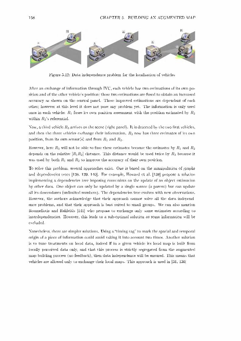
158 CHAPTER 5. BUILDING AN AUGMENTED MAP

Figure 5.12: Data independence problem for the localisation of vehicles

After an exchange of information through IVC, each vehicle has two estimations of its own po-

sition and of the other vehicle's position; these two estimations are fused to obtain an increased

accuracy as shown on the central panel. These improved estimations are dependant of each

other; however at this level it does not pose any problem yet. The information is only used

once in each vehicle: R1 fuses its own position assessment with the position estimated by R2

within R2's referential.

Now, a third vehicle R3 arrives on the scene (right panel). It is detected by the two rst vehicles,

and then the three vehicles exchange their information. R3 now has three estimates of its own

position, from its own sensor(s) and from R1 and R2.

However, here R3 will not be able to fuse these estimates because the estimates by R1 and R2

depends on the relative [R1R2] distance. This distance would be used twice by R3 because it

was used by both R1 and R2 to improve the accuracy of their own position.

To solve this problem, several approaches exist. One is based on the manipulation of graphs

and dependencies trees [138, 139, 140]. For example, Howard et al. [138] propose a solution

implementing a dependencies tree imposing constraints on the update of an object estimation

by other data. One object can only be updated by a single source (a parent) but can update

all its descendants (unlimited numbers). The dependencies tree evolves with new observations.

However, the authors acknowledge that their approach cannot solve all the data independ-

ence problems, and that their approach is best suited to small groups. We can also mention

Roumeliotis and Rekleitis [141] who propose to exchange only some estimates according to

interdependencies. However, this leads to a sub-optimal solution as some information will be

excluded.

Nonetheless, there are simpler solutions. Using a timing tag to mark the spatial and temporal

origin of a piece of information could avoid taking it into account two times. Another solution

is to tune treatments on local data, indeed in a given vehicle its local map is built from

locally perceived data only, and that this process is strictly segregated from the augmented

map building process (no feedback), then data independence will be ensured. This means that

vehicles are allowed only to exchange their local maps. This approach is used in [31, 136]

5.3. THEORETICAL FOUNDATIONS 159

5.3 Theoretical foundations

In this section, we will detail the theoretical foundations upon which our map-building ar-

chitecture is constructed; these include the (linear) Kalman Filter and the our approach to

Multi-Hypothesis Tracking (MHT) with the Dempster-Shafer Theory. Note that we will not

necessarily provide a detailed demonstration of the involved mathematics as some of them are

fairly common knowledge (notably the Kalman Filter). Adequate details will be provided for

important points or regarding our contribution to these theoretical foundations.

5.3.1 Kalman Filter

The Kalman Filter is a recursive algorithm allowing an estimation of unknown state variables

from a noisy series of measurements; it has been in use for several decades now [115, 116]. Both

discrete (the original) and continuous version exists; we will describe the discrete version only,

as we use discretised digital data. The lter is widely used for signal processing, notably in

data fusion, tracking or localisation applications.

It is able to output a statistically optimal (verifying the CramérRao bound) estimate on

the state of the underlying system, together with a variance-covariance matrix providing the

estimated accuracy of the lter. More precisely, its output will be optimal if (1) the process

model is linear and accurately matches the underlying real system, (2) the measurement and

process noises have a Gaussian distribution, and (3) the covariances of the noises are exactly

known.

The Kalman Filter is divided into two steps:

the prediction step, where the estimates of the state variables at the next time step, along

with their uncertainties, are computed based on an input (the control vector).

the update step, where the estimates are updated with measurements using a weighted

average, with more weight being given to estimates with higher certainty.

Before we describe the actual algorithm, we shall rst explain the dynamic model that is taken

into account by the Kalman Filter. The lter is based on linear dynamic systems discretised in

the time domain, which are modelled on a Markov chain built on linear operators perturbed by

Gaussian noises. The state of the system is represented as a vector of real numbers. At each

discrete time step, a noised linear operator is applied to the state to generate the new state

and some information from the controls on the system if they are known. Let us have the state

transition function f and the measurement function g; then the model can be written as:

Xk+1|k = f(Xk|k, uk, vk

)vk N (0, Rv, k) (5.1)

Zk+1 = g(Xk+1|k, nk

)nk N (0, Rn, k) (5.2)

where:

Xk+1|k is the real state vector at time k + 1 given the previous state vectors available up

to time k

160 CHAPTER 5. BUILDING AN AUGMENTED MAP

Zk+1 is the measured state vector at time k + 1

uk is the control vector

vk and nk are, respectively, the process and measurement noises, which are assumed to

be independent white Gaussian noises centred on zero, with positive variance-covariance

matrices Rv,k and Rn,k

As we said, the model can be represented by a Markovian Gaussian states model:

Xk+1|k = AkXk|k +Bkuk + vk vk N (0, Rv, k) (5.3)

Zk+1 = Ck+1Xk+1|k + nk+1 nk+1 N (0, Rn, k) (5.4)

where:

Ak is the state transition model from state Xk to Xk+1

Bk is the control-input model which is applied to the control vector uk

Ck+1 is the observation model (also the measurement matrix) which maps the true state

space into the observed space

From the previously described model, the Kalman Filter's goal is to compute an optimal es-

timate Xk+1|k+1 at time k + 1 of the real state vector, Xk+1|k+1, with the variance-covariance

matrix Pk+1|k+1. The lter is implemented using the two steps mentioned before, but not before

a rst initialisation step:

X0 = E [X0] = Z0 (5.5)

P0 = E[(X0 − X0

)(X0 − X0

)t]= Rn,0 (5.6)

Rv,0 = E[(v − v) (v − v)

t]

(5.7)

Rn,0 = E[(n− n) (n− n)

t]

(5.8)

Then, ∀kε [1, . . . ,+∞[, the steps are repeated (see also Fig. 5.13):

(1) Prediction step:

Xk+1|k = AkXk +Bkuk (5.9)

Pk+1|k = AkPkAtk +Rv,k (5.10)

(2) Update step:

Kk+1 = Pk+1|kCtk+1

[Ck+1Pk+1|kC

tk+1 +Rn,k+1

]−1(5.11)

Xk+1|k+1 = Xk+1|k +Kk+1

[Zk+1 − Ck+1Xk+1|k

](5.12)

Pk+1|k+1 = [I −Kk+1Ck+1]Pk+1|k (5.13)

5.3. THEORETICAL FOUNDATIONS 161

Figure 5.13: A graphical presentation of the Kalman Filter algorithm

Kk+1 is the Kalman gain; it is an optimal value that minimise the trace of Pk+1|k+1. In a three

dimensional localisation problem, the trace of Pk+1|k+1 is the sum of the variance on the x, y

and z axes, so minimising it means that the position estimate's certainty increases (this is also

said to mean that the lter is more informative).

The gain is used to weigh the relative condence in the predictions or measurements. Indeed

if Rn, the measurement noise variance-covariance matrix, is small, then Kk+1 will have a large

value. On the other hand, if Pk+1|k+1 is small, then Kk+1 will be small too. In the former case,

the Kalman Filter gives more credit to the measurements than the model, in the latter case the

lter gives more credit to the model than the measurements.

5.3.2 Multi-Hypotheteses Tracking using the Belief Theory

In section 5.2.2.3, we described the data association and tracking problem, and gave a few

references on methods to solve this problem. In the present section, we will present a multi-

hypotheses tracking (MHT) algorithm based on previous work by Mourllion et al. [142], Mourl-

lion [31]. This algorithm uses the Dempster-Shafer Theory (belief functions) to allow such

mutli-hypotheses tracking and is able to solve problematic associations that arose in previous

implementations of the theory. Belief functions provide an interesting formalism to manage and

handle imprecision, uncertainty and missing information. Instead of strictly considering prob-

ability distributions over a nite number of hypotheses, like the majority of other approaches,

belief functions are also computed over all subsets of hypotheses. A larger frame of discernment

than the one used in probability is then considered, allowing a better modelisation of doubt

when data is insuciently informative.

The algorithm described in this section combines the advantages of MHT (creation and destruc-

tion of objects) with a very high level of accuracy concerning target disappearance, allowing

it to discriminate between objects that have disappeared for good (by moving away of the

sensors' range) or being only temporarily invisible, because of occultations by another object

for example. This is achieved by solving issues related to the maximum global belief criterion,

allowing it to avoid problematic local associations that can arise while the global belief criterion

162 CHAPTER 5. BUILDING AN AUGMENTED MAP

is still satised.

We will provide here a formal description of the algorithm, where its implementation using

actual data is covered in section 5.4.3. However, at rst, we will give a general introduction to

the Dempster-Shafer Theory.

5.3.2.1 Introduction to Dempster-Shafer Theory

Belief functions were introduced by Dempster [123] in 1967 and further rened by Shafer [124]

in 1976, taking the name of the Dempster-Shafer Theory. It is also sometimes referred to as the

Belief Theory. Further extension was undertaken by Smets [143, 144] to create the Transferable

Belief Model (TBM).

At rst, we dene Ω, the universal set that represents the various possible states for the sys-

tem under consideration, i.e. the frame of discernment. The possible states are the simple

(singletons) acceptable propositions Hi, so that:

Ω = H1, H2, . . . ,Hn (5.14)

Hi ∩ Hj = Ø ∀i 6= j (5.15)

From this universal set, we can dene the power-set 2Ω that is the set of all subsets of Ω,

including the empty set ∅. The power-set includes all the combinations based on the hypothesisfrom the universal set. A proposition A can be a singleton hypothesis or a complex hypothesis,

which includes more than one hypothesis. ∅Ω represents impossible propositions (conicts) and

Ω the total ignorance, since it includes all existing hypothesis.

2Ω = A/A ⊆ Ω = ØΩ, H1, H2, . . . ,Hn, H1 ∪H2, . . . ,Ω (5.16)

In [145, 119, 146], the authors used an extended universal set Θ, the extended open world, by

creating a new hypothesis, labelled ∗ which representing any new hypothesis that is not initially

modelled in Ω. This approach allows discriminating between conict and new hypothesis, which

is not possible in the general approach.

Θ = H1, H2, . . . ,Hn, ∗ (5.17)

2Θ = ØΘ, H1, H2, . . . ,Hn, H1 ∪H2, . . . , ∗,Ω (5.18)

The Dempster-Shafer Theory allows to evaluate the likelihood of a proposition A through its

belief mass mΩ (A), the mass of elementary probability on the said proposition A, a function

dened as:

mΩ : 2Ω → [0, 1]

A → mΩ (A)(5.19)

The set of belief masses constitutes the basic belief assignment (BBA), which veries:

5.3. THEORETICAL FOUNDATIONS 163

mΩ (ØΩ) = 0 (5.20)∑A∈2Ω

mΩ (A) = 1 (5.21)

mΩ (A) is the degree of belief put in proposition A, more precisely it expresses the proportion

of all relevant and available evidence that supports the claim that the actual state belongs to

A but to no particular subset of A. mΩ (Ω) represents the mass of ignorance. If A is a complex

hypothesis (i.e. not a singleton one), it means that given the current state of knowledge on

the system, no mass could be assigned to a more specic proposition. This represents a partial

ignorance of the system's state. Total ignorance is represented by the following masses set:

mΩ (Ω) = 1 and mΩ (A) = 0 ∀A 6= Ω. The mass mΩ (ØΩ) is the mass of conict (the BBA is

labelled as normal ifmΩ (ØΩ) = 0), and propositions A that have a non-null mass (mΩ (A) > 0)

are called focal elements. When focal elements are composed only of singleton hypotheses, the

masses are linkable to probabilities, creating a set of Bayesian masses. If the extended open

world Θ is used, then, mΘ (ØΘ) +mΘ (∗) = mΩ (ØΩ).

From the mass assignments, we can dene the upper and lower boundaries of a probability

interval. This interval contains the precise probability of A (in the classical sense), and is

bounded by two non-additive continuous measures called belief and plausibility, so that:

bel (A) ≤ P (A) ≤ pl (A) (5.22)∑B|B⊆A

mΩ (B) ≤ P (A) ≤∑

B|B∩A6=ØΩ

mΩ (B) (5.23)

pl (A) = 1− bel(A)

(5.24)

where B is the set of propositions that implies A.

After the sets of mass assignments have been obtained, the problem becomes how to combine

two independent sets of mass assignments, in other words, how to combine evidence from

dierence sources (such as dierent sensors)? There are a number of dierent rules to do so,

the principal one being the Dempster-Shafer (DSR) rule.

Let us consider S information sources ∀A ⊂ Ω, which resulting BBA is mΩ1,...,S , called the joint

mass. Their respective focal elements are B1, . . . , BS . The DSR is computed so that the nal

mass of conict is null (mΩ1,...,S (ØΩ) = 0). The joint mass is given by:

mΩ1,...,S (A) =

1

K

∑B1∩...∩BS=A

mΩ1 (B1) . . .mΩ

S (BS) (5.25)

where K is a normalisation constant measuring the amount of conict between the sets, and

given by:

K = 1−∑

B1∩...∩BS=ØΩ

mΩ1 (B1) . . .mΩ

S (BS) (5.26)

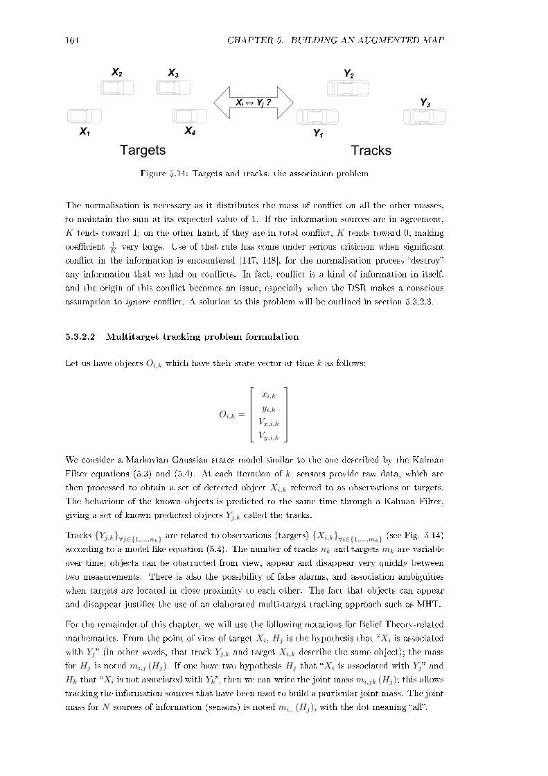
164 CHAPTER 5. BUILDING AN AUGMENTED MAP

Figure 5.14: Targets and tracks: the association problem

The normalisation is necessary as it distributes the mass of conict on all the other masses,

to maintain the sum at its expected value of 1. If the information sources are in agreement,

K tends toward 1; on the other hand, if they are in total conict, K tends toward 0, making

coecient 1K very large. Use of that rule has come under serious criticism when signicant

conict in the information is encountered [147, 148], for the normalisation process destroy

any information that we had on conicts. In fact, conict is a kind of information in itself,

and the origin of this conict becomes an issue, especially when the DSR makes a conscious

assumption to ignore conict. A solution to this problem will be outlined in section 5.3.2.3.

5.3.2.2 Multitarget tracking problem formulation

Let us have objects Oi,k which have their state vector at time k as follows:

Oi,k =

xi,k

yi,k

Vx,i,k

Vy,i,k

We consider a Markovian Gaussian states model similar to the one described by the Kalman

Filter equations (5.3) and (5.4). At each iteration of k, sensors provide raw data, which are

then processed to obtain a set of detected object Xi,k referred to as observations or targets.

The behaviour of the known objects is predicted to the same time through a Kalman Filter,

giving a set of known predicted objects Yj,k called the tracks.

Tracks Yj,k∀j∈1,...,nk are related to observations (targets) Xi,k∀i∈1,...,mk (see Fig. 5.14)

according to a model like equation (5.4). The number of tracks nk and targets mk are variable

over time; objects can be obstructed from view, appear and disappear very quickly between

two measurements. There is also the possibility of false alarms, and association ambiguities

when targets are located in close proximity to each other. The fact that objects can appear

and disappear justies the use of an elaborated multi-target tracking approach such as MHT.

For the remainder of this chapter, we will use the following notations for Belief Theory-related

mathematics. From the point of view of target Xi, Hj is the hypothesis that Xi is associated

with Yj (in other words, that track Yj,k and target Xi,k describe the same object); the mass

for Hj is noted mi,j (Hj). If one have two hypothesis Hj that Xi is associated with Yj and

Hk that Xi is not associated with Yk, then we can write the joint mass mi,jk (Hj); this allows

tracking the information sources that have been used to build a particular joint mass. The joint

mass for N sources of information (sensors) is noted mi,. (Hj), with the dot meaning all.

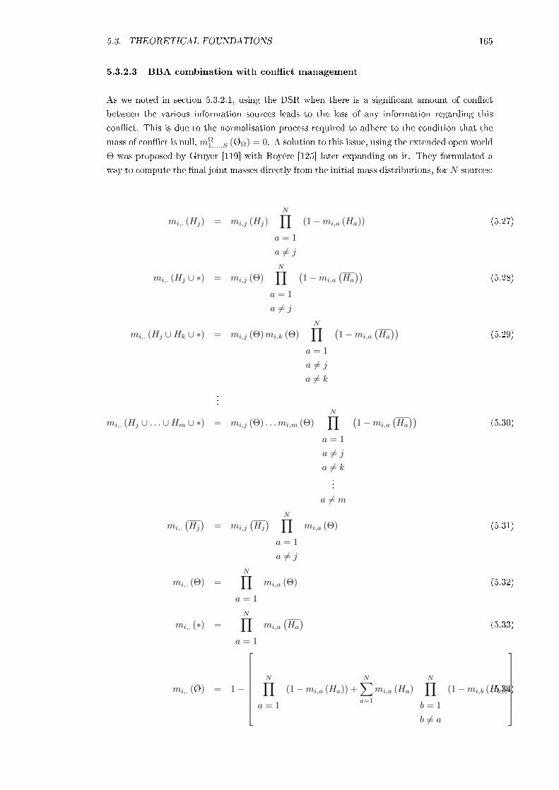
5.3. THEORETICAL FOUNDATIONS 165

5.3.2.3 BBA combination with conict management

As we noted in section 5.3.2.1, using the DSR when there is a signicant amount of conict

between the various information sources leads to the loss of any information regarding this

conict. This is due to the normalisation process required to adhere to the condition that the

mass of conict is null, mΩ1,...,S (ØΩ) = 0. A solution to this issue, using the extended open world

Θ was proposed by Gruyer [119] with Royère [125] later expanding on it. They formulated a

way to compute the nal joint masses directly from the initial mass distributions, for N sources:

mi,. (Hj) = mi,j (Hj)N∏

a = 1

a 6= j

(1−mi,a (Ha)) (5.27)

mi,. (Hj ∪ ∗) = mi,j (Θ)N∏

a = 1

a 6= j

(1−mi,a

(Ha

))(5.28)

mi,. (Hj ∪Hk ∪ ∗) = mi,j (Θ)mi,k (Θ)N∏

a = 1

a 6= j

a 6= k

(1−mi,a

(Ha

))(5.29)

...

mi,. (Hj ∪ . . . ∪Hm ∪ ∗) = mi,j (Θ) . . .mi,m (Θ)N∏

a = 1

a 6= j

a 6= k...

a 6= m

(1−mi,a

(Ha

))(5.30)

mi,.

(Hj

)= mi,j

(Hj

) N∏a = 1

a 6= j

mi,a (Θ) (5.31)

mi,. (Θ) =N∏

a = 1

mi,a (Θ) (5.32)

mi,. (∗) =N∏

a = 1

mi,a

(Ha

)(5.33)

mi,. (Ø) = 1−

N∏

a = 1

(1−mi,a (Ha)) +N∑a=1

mi,a (Ha)N∏

b = 1

b 6= a

(1−mi,b (Hb))

(5.34)

166 CHAPTER 5. BUILDING AN AUGMENTED MAP

Then, a Pignistic step is performed to share the masses of disjunction hypotheses (any of

Hj ∪ . . .∪Hm ∪∗) to the singleton hypotheses [125], as the disjunctions need to be removed for

the tracking process which is based, so far, on the assumption that a target can be associated

with only one single track. Pignistic probabilities have been coined by Smets [144] to describe

the assignation of regular probabilities to the possible options that can be taken for a given

decision, such as placing a bet1.

At rst, let us consider two observers looking at the same scene. The rst observer looks at the

potential associations between observed objects and known objects (Xi is associated with Yi)

and uses the extended universal set Θx = X1, . . . , Xm, ∗; the second observer looks at the

potential associations between the known objects and the observed objects (Yi is associated

with Xi) and uses the extended universal set Θy = Y1, . . . , Yn, ∗. Note that the number

of observers is not related to the number of sensors or sources of information. Indeed, if

we have only a single sensor, we will still consider two observers that are going to look for

associations between objects as explained before. From these two observers, we can create two

belief matrices with the Pignistic probabilities of association between tracks and targets. The

Pignistic probabilities are constructed as such:

P : 2Θ → [0, 1] (5.35)

P (A) =∑

B ∈ 2Θ

A ⊂ B

|A ∩B||B|

×m (B) (5.36)

P (Ø) = m (Ø) (5.37)

where |S| is the number of singletons elements in a set S, here A and B. The belief matrices

are:

Mpgi,. X1 · · · Xm

Y1 P1,. (Y1) · · · Pm,. (Y1)...

......

Yn P1,. (Yn) · · · Pm,. (Yn)

∗ P1,. (∗) · · · Pm,. (∗)Ø P1,. (Ø) · · · Pm,. (Ø)

Mpg.,j Y1 · · · Yn

X1 P.,1 (X1) · · · P.,n (X1)...

......

Xm P.,1 (Xm) · · · P.,n (Xm)

∗ P.,1 (∗) · · · P.,n (∗)Ø P.,1 (Ø) · · · P.,n (Ø)

1Quoting Professor Smets (emphasis ours), The transferable belief model is based on the assumption thatbeliefs manifest themselves at two mental levels: the `credal' level where beliefs are entertained and the 'pig-

nistic' level where beliefs are used to make decisions (from `credo' I believe and `pignus' a bet , both in Latin).Usually these two levels are not distinguished and probability functions are used to quantify beliefs at both levels.The justication for the use of probability functions is usually linked to 'rational' behavior to be held by an idealagent involved in some decision contexts.

5.3. THEORETICAL FOUNDATIONS 167

Then, we need to solve the possible contradictions or ambiguities that can be found between

these two matrices. If there is no contradictions, we have Pi,. (Yj) and P.,j (Xi) with the largest

values in their respective columns, and so on. Contradictions arise when the two matrices do not

associate the same objects together, such as when in Mpgi,. object X1 is associated with Y1 (the

probability P1,. (Y1) has the highest value) whereas inMpg.,j , object Y1 is associated withXm (the

probability P.,1 (Xm) has the highest value). Without ambiguities, all the probabilities in each

column are unique (in a single matrix). If ambiguities arise, there are two equal probabilities

in a same column; for example, in Mpgi,. , if P1,. (Y1) = P1,. (Yn).

To solve any of these two problems, Gruyer et al. [149] used a global Pignistic matrix and the

Hungarian Algorithm [150, 151] to nd the best optimal global association, according to the

maximum global belief criteria. Note that the global Pignistic matrix is only computed if there

are some ambiguities or contradictions in the two belief matrices. Otherwise, the associations

can be extracted from them directly (a decision is taken). If it is required, the global matrix

which is constructed from the two belief matrices is:

Mpgi,j Y1 · · · Yn ∗1 · · · ∗mX1 M1,1 · · · M1,n P1,. (∗) · · · 0...

......

...

Xm Mm,1 · · · Mm,n 0 · · · Pm,. (∗)∗1 P.,1 (∗) · · · 0 0 · · · 0...

......

...

∗n 0 · · · P.,n (∗) 0 · · · 0

with:

Mi,j =Pi,. (Yj) + P.,j (Xi)

2(5.38)

If we have three targets X1, X2, X3 and four tracks Y1, Y2, Y3, Y4, the nal decision process

can be visualised as such:

X1 X2 X3 ∗ ∗↓ ↓ ↓ ↓ ↓Y1 ∗ Y2 Y3 Y4

In that case, X1 is associated to Y1 and X3 is associated with Y2. X2 is associated with the ∗hypothesis, which mean it is a new object; a new track Y5 will have to be created in consequence

(added to the universal set Θ). The ∗ hypothesis is associated with Y3 and Y4, which means that

the two tracks have disappeared. They will not be deleted from the system's map immediately,

indeed targets that correspond to them might re-appear later because the objects are only

temporarily out of view. The system will keep them (the action is referred to as propagation)

and continue to process them for a certain time, by using a condence value. A new track has

its condence set to a value depending on the incertitude on its initial detection.

The condence belongs to [0, 1], it increases when there is a successful association, and decreases

when no targets can be associated with a track; when it reaches zero, the track is taken out

of the system. The lifespan of a track can be modulated depending on the function that is

168 CHAPTER 5. BUILDING AN AUGMENTED MAP

0 0.2 0.4 0.6 0.8 10

0.2

0.4

0.6

0.8

1

Co

nfi

den

ce

Normalised # of occurences

AssociationPropagation

Confidence at time t+1

Confidence at time t

Figure 5.15: Tracks' condence update process

used to increase/decrease condence. The simplest approach is to use a linear function (see

Fig. 5.15). Gruyer [119] proposed using Bezier curves to modulate the pessimism or optimism

of the tracking strategies, allowing it to maintain longer or, on the other hand, quickly remove

a track that is not associated with the targets anymore.

5.3.2.4 Multi-hypotheses tracking approach

Multi-Hypothesis Tracking (MHT) removes the previous assumption that a target can be asso-

ciated with only one track and vice versa. Indeed, this assumption can force a decision that is

incorrect. Abandoning the assumption of uniqueness has several benets. Now, the system

will be able to include multiple hypothesis in its decision (the equivalent of doubt), or, on the

contrary, reject any decision because the available data is of poor quality. This will prove useful

in a highly volatile environment such as on the road. Mourllion et al. [142], Mourllion [31]

proposed two methods to work with MHT, the Cascade and Threshold methods, each with

their specic advantages and disadvantages.

Cascade method Let us call the k-level hypotheses all the complex hypotheses (disjunctions)

composed of k singletons. We build belief matrices like on page 166, but using the normalisation

shown in Eq. (5.39) and (5.40); in that case the information on conict is lost.

P : 2Θ → [0, 1] (5.39)

P (A) =∑

B ∈ 2Θ

A ⊂ B

|A ∩B||B|

× m (B)

1−m (Ø)(5.40)

The Cascade method operates a recurring Pignistic repartition of masses from the k-level hypo-

theses to the (k − 1)-level hypotheses. It looks for the rst hypotheses (complex or singleton)

5.3. THEORETICAL FOUNDATIONS 169

that has a mass greater than 0.5 (if the belief mass on a hypothesis is greater than 0.5, it will

represent the belief maximum, since the sum of all masses is always equal to 1). Starting at the

highest k-level (i.e. Θ), the Cascade method spreads the masses from a k-level to the underlying

level, as long as it cannot nd a mass greater than 0.5. If a hypothesis has a mass greater than

0.5, it is propagated further down the processing chain. The Cascade method must run for all

targets currently available to the association process.

However, if the propagated hypothesis is complex, the Cascade method continues its spreading

of masses to obtain the weights that will be aected on that propagation. Indeed, if the method

returns the hypothesis H1 ∪ ∗, we need to know in which proportions the system believes H1

or ∗ are the correct.

If no mass greater than 0.5 can be found at any level, the Cascade method cannot take a

decision. However, it has not been designed to reject a decision. If there is no suitable mass

obtained from the Pignistic repartition, a reversed cascade is attempted, starting from the

smallest k-level and spreading mass to the higher (k + 1)-level.

Threshold method The Cascade method has two issues: (1) it is computationally complex,

and (2) it does not manage conict because the of the masses normalisation from Eq. (5.39)

and (5.40). To compensate for these issues, Mourllion et al. propose a second less complex

method, dubbed the Threshold method, which is considered superior (see Table 5.3 for their

respective advantages and disadvantages).

This time, the Mpgi,. and M

pg.,j Pignistic matrices (page 166) are used. For each line, a weighted

threshold t is computed according to Eq. (5.41), where kt ∈ [0, 1] is the weight.

ti = kt (1− Pi (Ø)) (5.41)

Any associations from the Pignistic matrices where probability is lower than t is ltered. The

value of weight kt can be used to control the number of hypotheses that pass through the

ltering process.

The smaller kt, the larger the number of hypotheses that can pass through the lter; in that

case, we have a cautious lter. This will lead to the creation of virtual tracks, that will

continue to be processed through future iterations until more information becomes available

and they are associated more precisely or disappear (they were false detections).

On the other hand, if kt ≥ 0.5 only a single hypothesis will be accepted at maximum. This

means that with these large values of kt, the ltering process will not allow any hypothesis

through. In other words, it means the association algorithm will reject taking any decision

on the hypotheses. Mourllion [31] recommends that this latter case should be used only for

computations internal to the association process, without aecting the overall decision taken

by the algorithm (upon which some critical upper-level systems might depend). The upside of

ltering a large number of hypotheses is that false alarms will be ltered in most situations.

If target Xi is associated to the two tracks Yj and Yk, two virtual tracks Y ∗ij and Y ∗ik are

actually created. The system is said to be doubting or hesitating on to which decision to take.

These virtual tracks are added to the universal set and will be processed by the system in

subsequent iterations, alongside normal tracks. The two tracks are likely to diverge, leading to

170 CHAPTER 5. BUILDING AN AUGMENTED MAP

Table 5.3: Comparison of the Cascade and Threshold MTH methods

Methods Cascade Threshold

Complexity High LowNumber of generated tracks Accurate InaccurateConict is accounted for? No Yes

Can reject decision? No Yes

the association of one with Xi and the other to the ∗ hypothesis. This latter track will see its

condence decrease until it is removed from the tracking system.

5.3.2.5 Conclusion

The augmented map building architecture described in section 5.4 allow the implementation of

either of these methods. It will be the rst time the whole MHT system is implemented in a

framework that will, eventually, be fed with actual on-vehicle sensors and IVC-received data.

5.4. BUILDING THE AUGMENTED MAP 171

5.4 Building the augmented map

In this section, we will describe the architecture we implemented to build an augmented map,

using the principles described in the previous section. The map-building architecture is set

within the SiVIC-RTMaps-based framework described in Chapter 4. It is hosted on both

software suites; however, most of the computing is performed within RTMaps. We will rst

give a general overview of the architecture, before explaining the three main stages in detail :

(1) spatial and temporal synchronisation, (2) association, and (3) fusion.

5.4.1 Global architecture

Fig 5.16 shows the overall high-level architecture of our map-building system. We limited

ourselves to a single information layer covering objects and their behaviour within a certain

area around the ego-vehicle, or the interest zone managed by a roadside server. The architecture

includes the three main stages described in the literature review, as well as the IVC module

and the local map-building modules. The architecture gives the point of view of a vehicle, with

a decentralised map-building approach, i.e. one where each vehicle (or road actor) computes

its own augmented map from local and remote data. In a centralised approach, the local map-

building modules would not necessarily be present, if the roadside server is not linked directly

to roadside sensors.

Fig 5.17 provides a more detailed view of the architecture. We will now explain each module's

function, before a more detailed presentation is given in the following subsections for each of

the three main stages.

Local map modules The local map modules are tasked with building the vehicle's local

map. The most simple case has a vehicle which only sensor is a positioning one (typically a

GPS). In this case, the local map contains only an object which describes the vehicle's location

and any available information on its type. Proprioceptive information, from an INS central

for example, can be used to enhance the vehicle's localisation. If the vehicle is equipped with

exteroceptive sensors, any object detected is included in the local map in a similar format as

the object describing the ego-vehicle.

The local map information is sent to both the synchronisation and IVC modules; the former

will update it to the current timestamp, if necessary, so it can be used to create the augmented

map, while the latter will format it appropriately and send it to other vehicles via the 802.11p

IVC simulation. This latter action involves passing information from RTMaps to SiVIC and

back.

IVC module The IVC module is based on the IVC simulation described in Chapter 4 and the

802.11p model from Chapter 3. It is principally located within SiVIC; information is exchanged

with modules in RTMaps through the shared memory and DDS mechanism. For more detail

on this module's functions, refer to Chapter 3, section 3.7 and Chapter 4, section 4.2.5.

Spatial and temporal synchronisation The spatial and temporal synchronisation module

receives information from the IVC module and the local map modules. It has three roles, each

performed by an independent sub-module (components).

172 CHAPTER 5. BUILDING AN AUGMENTED MAP

Figure

5.16:Overa

llaugmented

mapbuild

ingarch

itecture

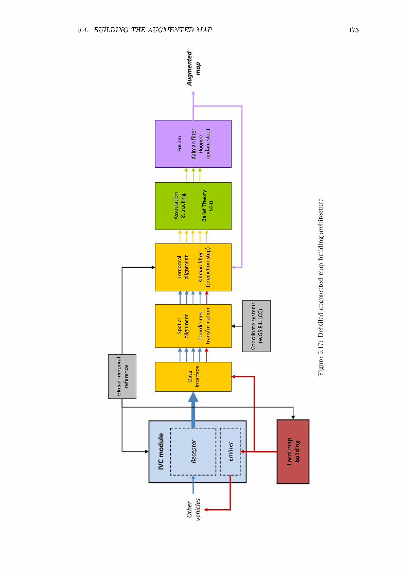
5.4. BUILDING THE AUGMENTED MAP 173

!

" #$%&

'( (

Figure

5.17:Detailed

augmentedmapbuildingarchitecture

174 CHAPTER 5. BUILDING AN AUGMENTED MAP

At rst, it must prepare the data received from remote sources and from the local map so that

they are all coherent. For that, the module decodes data that arrive from remote sources and

creates objects of a standardised format, so that the state vector of each object contains the

same elds ; this task is undertaken by the Data Interface component. Whether each eld is

lled with meaningful information depends on the data that was received from other vehicles.

The standardised state vector is:

X =

ID

S

A

tmin

tmax

T

X,Y, ZLLAX,Y, ZLAMVX , VY , VZLAMσXX , σY Y , σXY

E

C

Occ

(5.42)

The eld's signication are the following:

ID is the object's unique identier.

S is a boolean value used to described the object's state. It can take the following values:

0 = Inactive

1 = Ready to be used

2 = In use

3 = Synchronised

4 = Associated

5 = Fusion in progress

6 = Fused

A is a boolean value used to verify if the object is an augmented object (which is the case

when it is fed back from the augmented map).

tmin, tmax, T are timestamps. tmin and tmax can be used to follow the object's ow

through the architecture, to compute internal delays notably as well as expressing how

old the object is. T is the object's most recent timestamp in the common temporal

reference, that is used when its behaviour has to be predicted to what is considered the

current time. T is an 64-bits integer value expressing the number of microseconds elapsed

since January 1, 1970.

The triplets X,Y, ZLLA and X,Y, ZLAM give the object's position within two sets

of coordinate systems: X,Y, ZLLA in the GPS's reference WGS 84 coordinates, and

5.4. BUILDING THE AUGMENTED MAP 175

X,Y, ZLAM for a Lambert conformal conic projection-based coordinate system. Lambert-

like coordinates are used for the absolute referential in SiVIC, allowing the architecture

to accept data from real positioning systems or from simulated ones (such as the CarOb-

servers).

The triplet VX , VY , VZLAM gives the object's speed along the three axis, in Lambert

coordinates.

σXX , σY Y , σXY are elements of the object's variance-covariance matrix; the number of

elements might vary depending on whether the system is set to work in two dimensions

only (2× 2 matrix) or in three dimensions (3× 3 matrix).

E is an error code value that can be used to signal a problem with the object.

C gives the condence in the object's existence.

Occ records the number of occurrences (counted in loop iterations) for which the object

has been detected and tracked.

In a second time, the standardised objects are synchronised spatially by the Spatial Alignment

component. The component is tasked with verifying that all objects have a coordinate system in

common; the choice of which coordinate system to use is set by the user. If Lambert coordinates

are used globally, but one object only has its WGS 84 coordinates triplet lled, the component

will transform them to update the Lambert coordinates triplet.

Eventually, the standardised objects are temporally synchronised by the Temporal Alignment

component. To do so, the prediction step of a linear Kalman lter is used. The objects'

behaviour is evaluated to a common timestamp which is considered as the present time (all

objects will have the same value in eld T ). This timestamp is set the instant data enters

the component, and will not change in any downstream component. It will also be used as

the augmented map's timestamp. The Temporal Alignment receives feedback from the Fusion

module, so that objects in the augmented map are also aware of the new common timestamp.

Association & tracking The association and tracking module receives synchronised remote

and local objects as well as the previously synchronised augmented objects from the synchron-

isation module. Here, remote and local objects are associated with previously known augmented

objects, and if no match can be found, instructions are given to create new augmented objects.

The module also manages the disappearance of objects, that is when one augmented object

has not been associated with any remote or local object for a certain amount of time. . The

Multi-Hypothesis Tracking (MHT) algorithm described in Section 5.3.2 is used to perform this

task.

Fusion The last module performs the fusion of existing augmented objects with remote or

local objects, or the fusion of remote and local objects together to form new augmented ob-

jects, following the instructions received from the association and tracking module. This last

component uses the updated step of a linear Kalman lter, which is looped so that augmented

objects can be updated with data from the remote and local objects which are considered as

new measurements within the Kalman lter's formalism. The module outputs the augmented

objects forming the augmented map, using the same standardised state vectors as described

earlier.

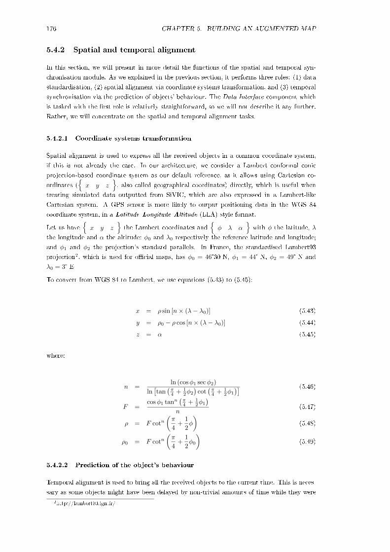
176 CHAPTER 5. BUILDING AN AUGMENTED MAP

5.4.2 Spatial and temporal alignment

In this section, we will present in more detail the functions of the spatial and temporal syn-

chronisation module. As we explained in the previous section, it performs three roles: (1) data

standardisation, (2) spatial alignment via coordinate systems transformation, and (3) temporal

synchronisation via the prediction of objects' behaviour. The Data Interface component which

is tasked with the rst role is relatively straightforward, so we will not describe it any further.

Rather, we will concentrate on the spatial and temporal alignment tasks.

5.4.2.1 Coordinate systems transformation

Spatial alignment is used to express all the received objects in a common coordinate system,

if this is not already the case. In our architecture, we consider a Lambert conformal conic

projection-based coordinate system as our default reference, as it allows using Cartesian co-

ordinates (x y z

, also called geographical coordinates) directly, which is useful when

treating simulated data outputted from SiVIC, which are also expressed in a Lambert-like

Cartesian system. A GPS sensor is more likely to output positioning data in the WGS 84

coordinate system, in a Latitude Longitude Altitude (LLA) style format.

Let us havex y z

the Lambert coordinates and

φ λ α

with φ the latitude, λ

the longitude and α the altitude; φ0 and λ0 respectively the reference latitude and longitude;

and φ1 and φ2 the projection's standard parallels. In France, the standardised Lambert93

projection2, which is used for ocial maps, has φ0 = 46°30 N, φ1 = 44° N, φ2 = 49° N and

λ0 = 3° E

To convert from WGS 84 to Lambert, we use equations (5.43) to (5.45):

x = ρ sin [n× (λ− λ0)] (5.43)

y = ρ0 − ρ cos [n× (λ− λ0)] (5.44)

z = α (5.45)

where:

n =ln (cosφ1 secφ2)

ln[tan

(π4 + 1

2φ2

)cot(π4 + 1

2φ1

)] (5.46)

F =cosφ1 tann

(π4 + 1

2φ1

)n

(5.47)

ρ = F cotn(π

4+

1

2φ

)(5.48)

ρ0 = F cotn(π

4+

1

2φ0

)(5.49)

5.4.2.2 Prediction of the object's behaviour

Temporal alignment is used to bring all the received objects to the current time. This is neces-

sary as some objects might have been delayed by non-trivial amounts of time while they were

2http://lambert93.ign.fr/

5.4. BUILDING THE AUGMENTED MAP 177

propagated in the wireless network, or in some overloaded software components. Additionally,

some objects might not have been updated for some time, yet they are still considered as ac-

ceptable by the downstream modules. The behaviour of these objects need to be predicted so

they can be associated with any new data relating to them that might have arrived in the mean

time. Eventually, for the downstream association and fusion to be meaningful, the objects need

to describe the state of the road scene in a single instant.

The estimator that we use to predict the evolution of objects at time tk+1based on their known

parameters at time tk is a linear Kalman Filter. The prediction stage, equations (5.9) and

(5.10), is the only part of the lter that is needed here.

Let us have ∆t = tk+1 − tk, the dierence between the current time tk+1 and the object's last

main timestamp (i.e. T ). ∆t will vary according to the object's nature. If the object is an

augmented object fed back from the latest augmented map, ∆t is the time elapsed since the

augmented map was last updated. If the object is a locally-perceived object, ∆t is the time

elapsed since it was detected by the exteroceptive sensors and updated in the local map. If

the object comes from the local map of another vehicle, exchanged over IVC, then ∆t is the

time elapsed since that local map was created; in that case, ∆t can be expressed as ∆t =

∆inf,e + ∆telecom + ∆inf,r, with ∆inf,e and ∆inf,r processing latencies in the emitter and

receptor, respectively, which include latencies in the local map building chain at the emitter

and data decoding and standardisation at the receptor; ∆telecom is the total latency introduced

in the IVC simulation.

To project the vehicle's behaviour to the current timestamp, we need a state-transition model,

which will give us the state-transition matrix Ak and the control-input matrix Bk. The state-

transition model is linear, since we are using a linear Kalman Filter. Hence, it will be a simple

two-dimensional state-transition model. Let us consider two options, that diers from the

nature of the control vector. The rst model uses the vehicle's acceleration for the control

vector, while the second model is simpler and uses the vehicle's speed for the control vector.

The state vectors are, respectively, X =[x y Vx Vy

]and X =

[x y

]. The state-

transition models are given by the equations (5.50) when using the acceleration for the control

vector, and equations (5.51) when using the speed for the control vector:

Xk+1|k 7→

xk+1 = xk + Vx,k∆t

yk+1 = yk + Vy,k∆t

Vx,k+1 = Vx,k + αx,k∆t

Vy,k+1 = Vy,k + αy,k∆t

(5.50)

Xk+1|k 7→

xk+1 = xk + Vx,k∆t

yk+1 = yk + Vy,k∆t

(5.51)

From these models, we can extract the state-transition and control-input matrices Ak and Bk

for the rst model:

Ak =

1 0 ∆t 0

0 1 0 ∆t

0 0 1 0

0 0 0 1

Bk =

0 0

0 0

∆t 0

0 ∆t

And similarly for the second model:

178 CHAPTER 5. BUILDING AN AUGMENTED MAP

Ak =

[1 0

0 1

]Bk =

[∆t 0

0 ∆t

]

The control vectors uk are, respectively, uk =[αx αy

]and uk =

[Vx,k Vy,k

].

We remind the Kalman Filter's prediction stage equations in (5.52) and (5.53). Filling them

with the vectors and matrices dened above, we obtain equations (5.54) to (5.57).

Xk+1|k = AkXk +Bkuk (5.52)

Pk+1|k = AkPkAtk +Rv,k (5.53)

Xk+1|k =

1 0 ∆t 0

0 1 0 ∆t

0 0 1 0

0 0 0 1

×

x

y

Vx

Vy

+

0 0

0 0

∆t 0

0 ∆t

×[αx

αy

](5.54)

Pk+1|k =

1 0 ∆t 0

0 1 0 ∆t

0 0 1 0

0 0 0 1

×

σx2 σyx σxVxσxVy

σxy σy2 σyVxσyVy

σxVxσyVx

σV 2x

σVxVy

σxVyσyVy

σVyVxσV 2

y

(5.55)

×

1 0 ∆t 0

0 1 0 ∆t

0 0 1 0

0 0 0 1

+

0.2 0 0 0

0 0.2 0 0

0 0 1 0

0 0 0 1

Xk+1|k =

[1 0

0 1

]×

[xk

yk

]+

[∆t 0

0 ∆t

]×

[Vx,k

Vy,k

](5.56)

Pk+1|k =

[1 0

0 1

]×

[σx2 σxy

σxy σy2

]×

[1 0

0 1

]+

[0.2 0

0 0.2

](5.57)

We shall use the second, simpler state-transition model withX =[x y

]and uk =

[Vx,k Vy,k

]for the remainder of this chapter. Note that since we use position data received from GPS-like

positioning system, the vehicle's position and speed are not accurately known. Thus, the initial

variance-coviariance matrix P0 must have non-null values on its diagonal.

5.4.3 Association and tracking

After the objects have been synchronised to tk+1, they need to be associated together to de-

termine which actual objects they represent. At this stage, we have objects coming from several

local maps through IVC, the targets, and the objects from the augmented map at time tk (if

tk 6= t0), coming through a feedback process, the tracks. They are associated using the 2-by-2

procedure described by Gruyer [119], and later expanded in the approach described in section

5.4. BUILDING THE AUGMENTED MAP 179

5.3.2.3. The association process' implementation is relatively complex, so to make it easier we

will not indulge into too much detail.

Given the targets X1, . . . , Xm and the tracks Y1, . . . , Yn, the double observers (see page

166) approach is used to compute the belief masses for each hypotheses Xi is associated with

Yj and Yi is associated with Xj, including the ∗ hypothesis (a new or lost object). The belief

mass sets are computed as follows, for an hypothesis Hj :

mi,j (Hj) =

0 if Ic,i,j ∈ [0, τ2]

Φ1 (Ic,i,j) if Ic,i,j ∈ [τ2, 1](5.58)

mi,j

(Hj

)=

Φ2 (Ic,i,j) if Ic,i,j ∈ [0, τ1]

0 if Ic,i,j ∈ [τ1, 1](5.59)

mi,j (Θ) =

1− Φ2 (Ic,i,j) if Ic,i,j ∈ [0, τ1]

1 if Ic,i,j ∈ [τ1, τ2]

1− Φ1 (Ic,i,j) if Ic,i,j ∈ [τ2, 1]

(5.60)

where Ic,i,j is the similarity index between target Xi and track Yj , which is based on a weighting

of the Mahalanobis distance between the target and tracks by their respective condence. τ1

and τ2 are thresholds used to alter the impartiality of the association. For example, for a

given value of mi,j (Hj), the association is optimistic if a low value of Ic,i,j is necessary, and

pessimistic if a high value of Ic,i,j is required. A simplied situation exists when τ1 = τ2, in

which case if τ1 = τ2 = 0.5 the association process is impartial, optimistic for τ1 = τ2 < 0.5 and

pessimistic for τ1 = τ2 > 0.5. The functions Φ1 and Φ2 are dened according to Eq. (5.61) and

(5.62), where τ = τ1 = τ2 and α is reliability index expressing the reliability of the information

source used to assess Hj .

Φ1 (Ic,i,j) =α

2

[1− cos

(πIc,i,j − τ

1− τ

)](5.61)

Φ2 (Ic,i,j) =α

2

[1 + cos

(πIc,i,jτ

)](5.62)

Then, the mass are combined and the Pignistic repartition and decision process from 5.3.2.3 is

applied; the output is a single association matrix. Let us have 7 targets X1, . . . , X7 and 5

tracks Y1, . . . , Y5, where object Y2 has disappeared from the scene and X5 and X7 correspond

to new objects never seen before. The initial association matrix is:

Y1 Y2 Y3 Y4 Y5 Y6 Y7

X1 1 0 0 0 0 0 0

X2 0 1 0 0 0 0 0

X3 0 0 1 0 0 0 0

X4 0 0 0 0 1 0 0

X5 0 0 0 0 0 1 0

X6 0 0 0 1 0 0 0

X7 0 0 0 0 0 0 1

180 CHAPTER 5. BUILDING AN AUGMENTED MAP

To make the matrix square, it was necessary to add to virtual objects Y6 and Y7. However,

note that Y6 is not associated with any target. This is because the association between X2

and Y2 is actually incorrect, its presence is a necessary consequence of the combination of the

belief matrices. However, it will disappear in a subsequent ltering process based on mi,. (∗)and m.,j (∗): the mass on the existing erroneous association is lower than the belief mass for

the ∗ hypothesis. The nal, ltered association matrix is:

Y1 Y2 Y3 Y4 Y5 Y6 Y7 ∗1 ∗2X1 1 0 0 0 0 0 0 0 0

X2 0 0 0 0 0 0 0 0 0

X3 0 0 1 0 0 0 0 0 0

X4 0 0 0 0 1 0 0 0 0

X5 0 0 0 0 0 0 0 0 1

X6 0 0 0 1 0 0 0 0 0

X7 0 0 0 0 0 0 0 1 0

One can see that Y2is not associated with anything, so it will either be ltered or propagated to

the next iteration, depending on its condence value. In our implementation, if the condence

drops under 0.2, the object is removed from the system. Note the two objects ∗1 and ∗2;they are new objects that will be created as new tracks, while the virtual tracks Y6 and Y7

are removed from the system. Virtual tracks or objects are always removed from the process,

even if new objects are being created for them, as it is the case here. A ltered version of the

above matrix (reduced to be Ntracks ×Ntargets, where Ntracks includes all the tracks that arepropagated, associated and created, here Ntracks = 6) is then passed on to the next stage in

the map-building process.

5.4.4 Fusion

Fusing the synchronised and associated objects together is the nal stage of the augmented

map creation. After fusion, the map will be left with updated or new augmented objects. A

simple way to fuse associated objects together is to compute the average of their state vectors'

variables. However, this process is not the most optimal. A better approach is using the update

stage of the linear Kalman lter, especially so since we used the predictive stage for temporal

synchronisation. The equations pertaining to the Kalman Filter's update stage are given in

equations (5.63) to (5.65); however, they need to be adapted to our problem.

Kk+1 = Pk+1|kCtk+1

[Ck+1Pk+1|kC

tk+1 +Rn,k+1

]−1(5.63)

Xk+1|k+1 = Xk+1|k +Kk+1

[Zk+1 − Ck+1Xk+1|k

](5.64)

Pk+1|k+1 = [I −Kk+1Ck+1]Pk+1|k (5.65)

The standard lter consider the estimate Xk+1|k and will associate it with a measurement Zk+1

to form an updated estimate Xk+1|k+1. In our setting, we rstly considered that Xk+1|k is

the synchronised augmented object X0,k+1|k, which will serve as the anchor for the fusion

process. We have a number of other objectsX1,k+1|k . . . Xi,k+1|k

associated with the

augmented object. We consider that these objects are our new measurements, so that:

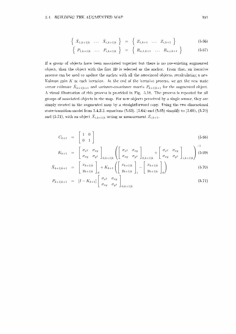
5.4. BUILDING THE AUGMENTED MAP 181

X1,k+1|k . . . Xi,k+1|k

=

Z1,k+1 . . . Zi,k+1

(5.66)

P1,k+1|k . . . Pi,k+1|k

=

Rn,1,k+1 . . . Rn,i,k+1

(5.67)

If a group of objects have been associated together but there is no pre-existing augmented

object, than the object with the rst ID is selected as the anchor. From that, an iterative

process can be used to update the anchor with all the associated objects, recalculating a new

Kalman gain K at each iteration. At the end of the iterative process, we get the new state

vector estimate Xk+1|k+1 and variance-covariance matrix Pk+1|k+1 for the augmented object.

A visual illustration of this process is provided in Fig. 5.18. The process is repeated for all

groups of associated objects in the map. For new objects perceived by a single sensor, they are

simply created in the augmented map by a straightforward copy. Using the two dimensional

state-transition model from 5.4.2.2, equations (5.63), (5.64) and (5.65) simplify to (5.69), (5.70)

and (5.71), with an object Xi,k+1|k acting as measurement Zi,k+1.

Ck+1 =

[1 0

0 1

](5.68)

Kk+1 =

[σx2 σxy

σxy σy2

]0,k+1|k

[ σx2 σxy

σxy σy2

]0,k+1|k

+

[σx2 σxy

σxy σy2

]i,k+1|k

−1

(5.69)

Xk+1|k+1 =

[xk+1|k

yk+1|k

]0

+Kk+1

([xk+1|k

yk+1|k

]i

−

[xk+1|k

yk+1|k

]0

)(5.70)

Pk+1|k+1 = [I −Kk+1]

[σx2 σxy

σxy σy2

]0,k+1|k

(5.71)

182 CHAPTER 5. BUILDING AN AUGMENTED MAP

2 4 6 8 10 12 14 16 18 20 222

4

6

8

10

12

14

16

18

X axis (metres)

Y a

xis

(met

res)

(a) Four associated objects and their respective variance ellipsoids

2 4 6 8 10 12 14 16 18 20 222

4

6

8

10

12

14

16

18

X axis (metres)

Y a

xis

(met

res)

(b) The same four objects, overlaid with the fused augmented object and its varianceellipsoid (magenta)

Figure 5.18: Illustration of the fusion process for an augmented object

5.5. PERFORMANCE EVALUATION 183

5.5 Performance evaluation, cooperative versus non-cooperative

In this section, we will analyse data collected using our augmented map-building architecture, in

order to compare its performance versus non-cooperative perception. Given the overall context

of this thesis, this performance comparison will not be made in terms of classic performance

criteria for algorithms. Rather, we will look into the improvements that CS can bring to the

performance of risk assessment. To do so, we will use a classic risk criterion based on the Time

to Collision (TTC) metric; further details on how this will be adapted for our scenario are given

in 5.5.2. The limitations introduced in the augmented map-building process by limitations of

the underlying layers, specically from telecommunications as investigated in Chapter 3, will

be accounted for in this study.

5.5.1 Scenario

We used our reference vehicles string scenario, as presented in Chapters 2 and 4; the setup is

actually identical to the non-repeatable scenario described in section 4.4. A ve-vehicle string

(1 leader, 4 followers) is set up in SiVIC, starting from grouped positions at one location on the

test track. From these start positions, the vehicles arrange themselves in a string on the right-

hand lane and progressively speed up to 70 km/h. The eet is still homogeneous to simplify the

scenario, with tinter = 2.5 seconds; this latter value simulates a medium density string where

drivers drive according to classic safety recommendations (i.e. maintaining at least 2 seconds

of intervehiculary time). The drivers' reaction time is th = 0.5 second.

To create a risky driving situation, we use the emergency braking event also used in Chapter

4. The lead vehicle performs an emergency braking manoeuvre about 700 metres from the

start position, in a straight section of the track. EEBL systems are not equipped on any of the

vehicles, so they only react according to the instructions outputted by the controller described

in Chapter 4. We consider two sub-scenarios in terms of CS equipment:

1. No CS-equipped vehicles in the string. However, veh5 is tted with a set of exteroceptive

(laserscanner) and localisation sensors to build a map of its immediate environment; this

map is used to compute a risk indicator for the driving situation relatively to veh5.

2. All vehicles are CS-equipped, they broadcast their position to each other. All vehicles

will build an augmented map from local positioning data and the information received

from the other vehicles, for example, in veh5, an augmented map is built from local data

and information from veh1,...,4. The maps are then used to compute a risk indicator for

the driving situation relative to ego-vehicle. A number of variations to the scenario will

be considered, relating to the frequency at which data is broadcasted to other vehicles.

5.5.2 Risk indicator

In order to compare the interest of CS versus non-cooperative systems in a risk assessment

context, we need a unique risk criterion or measurement metric. Over the years, a number of

approaches have been proposed to measure the risk of a given driving situation (examples are

listed in [152]), with a common thread: the risk indicator must be simple enough to be easily

understood by drivers, and yet convey an appropriate and representative estimation of the risk

and danger of the driving situation. For this study, we will use the most common risk metric,

184 CHAPTER 5. BUILDING AN AUGMENTED MAP

0 5 10 150

0.2

0.4

0.6

0.8

1

TTC (seconds)

Ris

k ([

0,1]

)

Ammoun, 2007Glaser et al., 2010

Figure 5.19: Risk functions from two studies using TTC

the Time to Collision (TTC). Note that TTC is used to get an instantaneous risk which is

re-computed at all times, there is no notion of a duration of operations over which the risk

could accumulate (exposure).

The TTC is a projection of the time remaining at time t before a future collision between two

vehicles, if they do not change their driving behaviour (which is speed, acceleration or direction

of driving). It is compared to the driver's reaction time, if the TTC is smaller than his reaction

time, crash is inevitable. If the TTC is small, but not smaller than the driver's reaction time,

substracting the two values can give the remaining time for the driver, or an automated crash

avoidance system, to perform avoidance actions. On the other hand, if the crash is indeed

inevitable, there might still be enough time for mitigation actions to take place, such as an

emergency braking manoeuvre to reduce the vehicle's speed at the expected collision time. As

seen in Chapter 4, fatality and injury rates are directly related to the speed of impact between

two objects on the road. TTC is actually a surrogate of risk; indeed, risk is usually considered

as a combination of the probability for an event to happen and of the gravity of said event. In

terms of road safety, the instantaneous crash risk is thus the probability of crash multiplied by

the expected severity of said crash, if it were to occur.

The probability of crash can be computed from the TTC through a function, such as from

[153, 154] which are shown in Fig. 5.19. In the case of Ammoun [153], the crash probability

is directly indicative of risk; on the other hand, for Glaser et al. [154] the probability obtained

from the TTC is then multiplied by a severity value. The severity is obtained in a similar

process that we get the relationship between severity and EES in the previous chapter. In Fig.

5.19, the two functions are both linear functions that assign a maximum risk/crash probability

when the TTC is under a certain threshold (1 or 2 seconds) and no risk/probability at all (or

a very small constant value) when it is above a certain threshold (10 or 5 seconds).

Despite its popularity, TTC is not always the most relevant indicator. For example, when

two vehicles drives at the exact same speed, their TTC value would be high, leading to a low

risk. However, if the vehicles are driving at this same speed but within less than 20 metres,

5.5. PERFORMANCE EVALUATION 185

for example, from each other, the TTC will still be high, although this situation is clearly

dangerous: the following vehicle would have no time to react to any event presented by the lead

vehicle. To circumvent this problem, previous studies usually couple TTC with other values.

For example, Glaser et al. [154] use the intervehicular time, and build a risk function based on

that metric.

In a simple, two-vehicle situation, the TTC can be used directly, from the point of view of

the following vehicle. However, when we start to consider augmented perception, there will be

more objects inside the ego-vehicle eld of view. This should allow building a more complex

representation of the driving risk for the ego-vehicle but also for a given driving situation.

Let us have a string of n vehicles veh1, . . . , vehn, where the ego-vehicle (the only one that canhave exteroceptive sensors) is vehn. Note that the process we will explain actually takes place in

all other vehicles when they are equipped with the cooperative risk assessment system; we will

describe the process only from the point of view of vehn to limit cluttering. The TTC TTCn−1

with the immediately preceding vehicle (vehn−1) is computed to represent a risk-assessment

system based on a mono-vehicle system. Simultaneously, we will also evaluate risk through the

augmented map in order to easily compare the outputs of the two systems. To do so, we use

several steps.

At rst, the TTC regarding all of the known objects in the augmented map and the ego-vehicle

vehn are computed: TTC1,n, . . . , TTCn−1,n. Then, using the function f from Glaser et al.

[154] (shown in Fig. 5.19 as the red curve), we compute a crash probability Pi,n for each

vehicle i ∈ [1, n− 1]. Then, the risk Ri,n for each vehicle is computed according to Eq. (5.73),

where g is a function that computes the severity of the potential crash using the EES and

G, which is the transfer function linking the EES to the likelihood of injury or death, built

from an analysis of car crash databases. Note that here, we will consider only the likelihood

of severe injury or death, the most pessimistic scenario; G would change if one considers the

likelihood of, for example, mild injuries. The EES is computed with Eq. (5.75), where for a

vehx, Vx is its speed (at the impact, the same as used for the TTC if nothing changes) and

mx its mass. We actually take the maximum between the two values computed with g to

represent two variations of the same crash: g (Vn, Vi) represents the severity of a crash where

the two involved vehicles have not changed their speed compared to the current time; on the

other hand, g (Vn, Vi − γTTCi,n) represents the severity of the crash that would happen if vehi

was to perform a sudden emergency braking manoeuvre with deceleration γ (γ w 0.8g in our

implementation), which is closer to the actual conditions of the scenario. That way, the most

pessimistic risk assessment is prepared for.

Pi,n = f (TTCi,n) (5.72)

Ri,n = Pi,n ×max [g (Vn, Vi) , g (Vn, Vi − γTTCi,n)] (5.73)

g (Vn, Vi) = G (eesi,n) (5.74)

eesi,n = (Vn − Vi)mi

mi +mn(5.75)

In our test scenario, we will have four objects plus the ego-vehicle from which the driving scene

will be considered. This means that in the non-cooperative application, we will only have one

risk R4,5 since veh5 is only capable of sensing veh4 which is in front of it, blocking the view to the

other vehicles. In the cooperative application, we have an array of risk R1,5, R2,5, R3,5, R4,5

186 CHAPTER 5. BUILDING AN AUGMENTED MAP

for veh5, but also for all the other vehicles, as such: Rj,i, . . . , Rn,i where j ∈ [1, n] , j 6= i .

Next, we combine these risks to obtain the global risk Rg,i as perceived by a single vehicle vehi.

The total global risk pertaining to the driving situation as perceived by all vehicles isRg; the

higher Rg, the more dangerous the driving situation (see the results section for further details

on how the Rg,i and Rg are computed).

5.5.3 Results

We implemented the scenario in our architecture, running both the cooperative and non-

cooperative risk assessment processes at the same time. The maps produced by the local

and augmented perception systems are shown in Fig. 5.20, when the string was formed. We

used a standardised representation where the objects themselves are squares centred upon the

object's absolute position; they are surrounded by their incertitude ellipsoids (build from the

variance-covariance matrix) which represented the area within which there is a 0.9 probability

that the object was located. A white line was used to represent the speed vector, in m.s−1,

which is shown to scale.

The following parameters were used:

veh1, . . . , veh4 sent their positioning data every 500 ms, with a latency of no more than

5 ms.

veh5 updated its own position every 100 ms.

veh5 created a local map every 50 ms and an augmented map every 100 ms.

Firstly, let us study the risk assessment performed with the local map. As mentioned before,

only R4,5 was available since veh5 was only capable of sensing veh4 with its front-facing laser-

scanner. On Fig. 5.21a and Fig. 5.21b we present TTC4,5, P4,5 and R4,5, the time to collision,

probability of collision and risk computed for veh4, for two simulated runs (henceforth: A and

B).

In both case, we noticed that the risk starts to increase after a plateau of about 10 to 5 seconds

before the crash; this corresponds to a reduction of TTC4,5; TTC4,5 had previously remained

stable for half a dozen of seconds. TTC4,5 starts to decrease as veh4 is pressing the brakes and

veh5 is still driving toward it a full speed. Interestingly, R4,5 was relatively lower during the

rst half of the scenario despite a large value of P4,5, in both A and B. This can be explained

as such: at the beginning, even if the crash probability rises, the risk value decreases because

the vehicles are driving relatively slowly and moving away from each other; thus, the severity

value decreases, taking R4,5 down with it.

Let us have a threshold of Rx = 0.7 to say that the driving situation is dangerous. With local

perception only, the driver will be warned about 5 seconds before the actual crash. This is a

short advance warning time, but it would be enough for the driver to prepare for a dangerous

event and initiate some mitigation or avoidance manoeuvre (at the speed of the scenario). Note

that in both runs there is a brief instant (after the 40 and 50-second marks, respectively) where

the situation would be agged as dangerous because R4,5 is above the threshold.

Now, we want to compare the performance of the local risk assessment to an augmented-

perception based approach. We need to compute Rg, which represent the risk for the whole

5.5. PERFORMANCE EVALUATION 187

(a) Local map built by veh5 using exteroceptive sensors and its GPS only;veh4 is visible, as well as a ghost object (on the left, which is most likelya misidentication of a ground reection) that has not been ltered out ofthe system yet.

(b) Raw information present at the beginning of the augmented map build-ing process in veh5: in red, the latest available objects received from othervehicles as well as from veh5's GPS; in green the augmented objects alreadyknown, fed-back from the previous loop. Here, there is a signicant dier-ence between the augmented and received objects because the image wascaptured well into the 500 ms GPS update cycle.

(c) The augmented map built by veh5 with data received from the othervehicles and its local positioning data.

Figure 5.20: Visualisations of the local and augmented map

188 CHAPTER 5. BUILDING AN AUGMENTED MAP

25 30 35 40 45 50 55 600

0.1

0.2

0.3

0.4

0.5

0.6

0.7

0.8

0.9

1Run #A

Time (seconds)

Ris

k −

Cra

sh p

roba

bilit

y

25 30 35 40 45 50 55 600

1

2

3

4

5

6

7

8

9

10

TT

C (

seco

nds)

TTC

Crash probabilityRisk

(a) Variables for run A

30 35 40 45 50 55 60 65 700

0.1

0.2

0.3

0.4

0.5

0.6

0.7

0.8

0.9

1Run #B

Time (seconds)

Ris

k −

Cra

sh p

roba

bilit

y

30 35 40 45 50 55 60 65 700

1

2

3

4

5

6

7

8

9

10

TT

C (

seco

nds)

Crash probabilityRisk

TTC

(b) Variables for run B

Figure 5.21: Local measurements of TTC, crash probability and subsequent risk

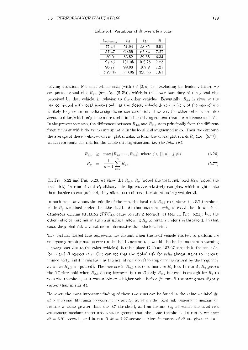
5.5. PERFORMANCE EVALUATION 189

Table 5.4: Variations of dt over a few runs

twarning tA tL dt

47.29 51.94 58.85 6.9157.27 60.55 67.82 7.2750.0 53.52 59.86 6.3497.45 101.05 108.28 7.2396.77 99.93 107.2 7.27379.85 383.05 390.66 7.61

driving situation. For each vehicle vehi (with i ∈ [2, n], i.e. excluding the leader vehicle), we

compute a global risk Rg,i (see Eq. (5.76)), which is the lower boundary of the global risk

perceived by that vehicle, in relation to the other vehicles. Essentially, Rg,i is close to the

risk computed with local sensors only, as the closest vehicle driven in front of the ego-vehicle

is likely to pose an immediate signicant source of risk. However, the other vehicles are also

accounted for, which might be more useful in other driving context than our reference scenario.

In the present scenario, the dierences between R4,5 and Rg,5 stem principally from the dierent

frequencies at which the tracks are updated in the local and augmented map. Then, we compute

the average of these vehicle-centric global risks, to form the actual global risk Rg (Eq. (5.77)),

which represents the risk for the whole driving situation, i.e. the total risk.

Rg,i ≥ max (Rj,i, . . . , Rn,i) where j ∈ [1, n] , j 6= i (5.76)

Rg =1

n− 1

n∑i=2

Rg,i (5.77)

On Fig. 5.22 and Fig. 5.23, we show the Rg,i, Rg (noted the total risk) and R4,5 (noted the

local risk) for runs A and B ; although the gures are relatively complex, which might make

them harder to comprehend, they allow us to observe the situation in great detail.

In both runs, at about the middle of the run, the local risk R4,5 rose above the 0.7 threshold

while Rg remained under that threshold. At that moment, veh5 assessed that it was in a

dangerous driving situation (TTC4,5 came to just 2 seconds, as seen in Fig. 5.21), but the

other vehicles were not in such a situation, allowing Rg to remain under the threshold. In that

case, the global risk was not more informative than the local risk.

The vertical dotted line represents the instant when the lead vehicle started to perform its

emergency braking manoeuvre (in the EEBL scenario, it would also be the moment a warning

message was sent to the other vehicles); it takes place 47.29 and 57.27 seconds in the scenario,

for A and B respectively. One can see that the global risk for veh2 almost starts to increase

immediately, until it reaches 1 at the actual collision (the step eect is caused by the frequency

at which Rg,2 is updated). The increase in Rg,2 starts to increase Rg too. In run A, Rg passes

the 0.7 threshold when Rg,3 do so; however, in run B, only Rg,2 increase is enough for Rg to

pass the threshold, as it was stable at a higher value before (in run B the string was slightly

denser than in run A).

However, the most important nding of these two runs can be found in the value we label dt;

dt is the time dierence between an instant tL, at which the local risk assessment mechanism

returns a value greater than the 0.7 threshold, and an instant tA, at which the total risk

assessment mechanism returns a value greater than the same threshold. In run A we have

dt = 6.91 seconds, and in run B dt = 7.27 seconds. More instances of dt are given in Tab.

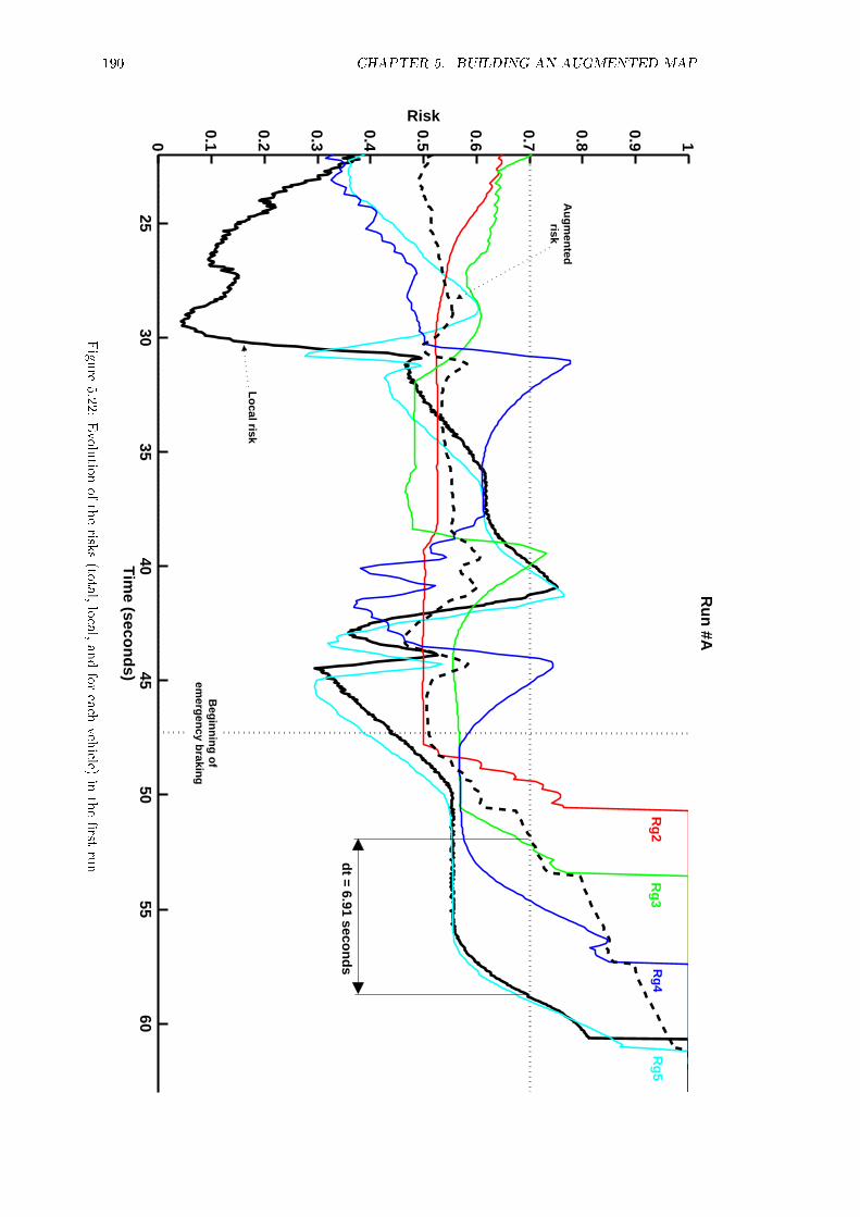
190 CHAPTER 5. BUILDING AN AUGMENTED MAP

2530

3540

4550

5560

0

0.1

0.2

0.3

0.4

0.5

0.6

0.7

0.8

0.9 1R

un

#A

Tim

e (secon

ds)

Risk

dt = 6.91 seco

nd

s

Beg

inn

ing

of

emerg

ency b

raking

Lo

cal risk

Au

gm

ented

risk

Rg

2R

g3

Rg

4R

g5

Figure

5.22:Evolutio

noftherisk

s(to

tal,local,andforeach

vehicle)

intherst

run

5.5. PERFORMANCE EVALUATION 191

3035

4045

5055

6065

700

0.1

0.2

0.3

0.4

0.5

0.6

0.7

0.8

0.91

Ru

n #

B

Tim

e (s

eco

nd

s)

Risk

dt

= 7.

27 s

eco

nd

s

Beg

inn

ing

of

emer

gen

cy b

raki

ng

Au

gm

ente

dri

sk

Lo

cal r

isk

Rg

3R

g4

Rg

2R

g5

Figure

5.23:Evolutionoftherisks(total,local,andforeach

vehicle)in

thesecondrun

192 CHAPTER 5. BUILDING AN AUGMENTED MAP

0 50 100 150 200 250 300 350 4000

0.05

0.1

0.15

0.2

0.25

0.3

0.35

0.4

0.45

0.5

Range (metres)

Fra

me

loss

rat

io

Maximum frame loss envelop (for 1,000 generations)Average frame loss

Figure 5.24: Example of the repartition of vehicles in the string, just before the emergencybraking, compared to the average and envelop of frame loss

5.4. We see that over these runs, dt was always larger than 6 seconds. This means that further

than the 5 seconds, at most, of advance warning given just by the local perception, we can now

have a total advance warning of 11 to 13 seconds by using augmented perception. The driver

of veh5 can be warned in advance of an issue taking place further in the string before it has the

capability to become aware of it. Although in our scenario the implementation did not include

a driver reaction driven by the risk assessment process, the advance warning would allow veh5

to prepare in several ways: the driver's reaction time can be shortened by its enhanced state

of alertness, and the vehicle's speed would likely be reduced. Altogether, the driver would

most probably be able to avoid a rear-end crash with veh4, even without the presence of an

EEBL-like CCW system.

The results above were obtained with non-perfect IVC, modelled according to our empirical

model from Chapter 3. Within the scenario's conditions, IVC imperfections appeared not to

be a hindrance to the timely output of a warning signal when Rg passes the danger threshold.

This can be partially attributed to the short-to-medium range at which V2V communications

were taking place in the scenario.

Indeed, the vehicles string is spread over a distance of 250 to 300 metres at most, with inter-

distances varying from 30 to 60+ metres. An example centred on the rst vehicle is shown in

Fig. 5.24, with a 220-metres-long string; in these conditions, the average frame loss is less than

5%, the only signicant area where frames can be lost at a higher rate is the ground-reection

area. Note that this graph applies only to the rst vehicle. From the point of view of veh3,

both veh1 and veh5 are located within the ground-reection interference area. Latency is not

aected by range, but the size of the frames exchanged between vehicles is at most 0.5 kilobyte,

meaning latency will be 9 to 12 milliseconds on average.

The most obvious limitation of this system is that the rst few vehicles in the string will usually

not benet from the enhanced risk assessment process. For example, in run A, veh4 would have

an advanced warning of only 2.71 seconds compared to its local perception; the local and total

5.5. PERFORMANCE EVALUATION 193

risk as seen from veh3 would cross the 0.7 threshold at the same time and veh2 would only

receive an advance warning from the augmented perception after the actual crash, defeating its

purpose. On the other hand, in run B, veh3, veh4 and veh5 would receive an advance warning

of respectively 2.5, 5.06 and 7.27 seconds; only veh2 would not benet from the system.

194 CHAPTER 5. BUILDING AN AUGMENTED MAP

5.6 Conclusion

The aim of this chapter was, at rst, to design and implement an architecture for building

an augmented map using the SiVIC-RTMaps framework, and, secondly, to show that it can

perform better than a non-cooperative approach to assess the risk of a driving situation within

our reference scenario.

Before tackling any of this chapter's goals, we oered a literature review covering several related

subjects from multi-sensors data fusion and the construction of local maps to the construction

of augmented maps. Afterwards, we provided the theoretical foundations upon which our map-

building architecture is based. After presenting the renowned Kalman Filter, we expended on

our association approach, which is based on the Belief Theory. The Belief Theory oered a good

compromise in terms of accuracy and processing requirements compared to other, essentially

probabilistic, methods. Furthermore, it is capable of managing the apparition of new objects

and the disappearance of older ones, which is required in the highly changing road environment.

We detailed a Multi-Hypothesis Tracking algorithm that is based on early works undertaken

at the LIVIC laboratory, and for which we provided the rst actual implementation in our

map-building system.

Then, we presented the design of our actual map-building architecture. This architecture took

full advantage of the SiVIC-RTMaps framework and of the CS-simulation architecture, that we

developed in Chapter 4. In terms of actual programming, the two architectures exist side-by-side

and exchange data wherever and whenever necessary. Objects' parameters are extracted from

the SiVIC-side of the CS-simulation architecture and passed on to the map-building modules.

It is important to stress out that our map-building architecture is not limited to simulated data

from SiVIC. Indeed, it is transparent to the origin of input data and can be deployed easily

with data collected on actual vehicles with real sensors (this is facilitated by using RTMaps).

A few examples of the architecture's output were presented to illustrate the type of map it can

build, as well as the dierent stages of the building process.

We then implemented a simple risk assessment system based on a combination of the crash

probability obtained from the TTC, and the expected severity of the probable crash, obtained

from the EES. By combining dierent appropriate risk values, we extracted the global risk as

perceived by a vehicle depending on whether it used only local sensors or had access to the

augmented map. We chose to put our focus on the last vehicle of a 5-vehicle string, in order to

compare the two approach in an emergency breaking scenario (the same as in Chapter 4).

Our results showed that the local risk-assessment system can inform the drivers that they are

entering "dangerous" driving conditions with at most 5 seconds of warning before the actual

crash, in the case of an emergency braking manoeuvre in our vehicles string scenario. On the

other hand, the augmented-map based risk-assessment system only gives an additional 2 to 7

seconds of advance warning, for a total of almost 13 seconds of warning before the crash, in the

best case scenario (for the string's last vehicle). The advance warning remained consistent over

several runs of the same non-repeatable scenario, with varying intervehicular distances in each

string.

These results were obtained with the IVC simulation from Chapter 3, that accounts for real-

istic frame loss and latency. It showed that, within the limits of the vehicles string, IVC

imperfections did not have a signicant eect on the augmented map's risk assessment capab-

ility. Imperfections might have a more signicant eect at longer ranges; however, the relative

5.6. CONCLUSION 195

speed between the vehicles is small (under normal driving conditions), so the very low speed

and low speed classes of our frame loss model would be used most of the time (see Fig. 3.40

in Chapter 3). With this model's calibration, any signicant eect of frame loss would be felt

only 350 to 400 metres away from the emitter. The ve-vehicle string is only 250 to 300 metres

long, meaning that frame loss was relatively limited (but non-zero, and sometimes subject to

the ground-reection interferences). Latency is not aected by range, and would have been 5

to 10 milliseconds, given the size of the exchanged frames. A perfect system would probably

have yielded better results. However, such results would not be representative of what would

happen on an actual road when compared to our current results.

We argue that this additional time would be largely sucient for a driver faced with such an

emergency scenario to adapt their behaviour and prepare for the incoming "braking wave"; it

is likely that the driver of the fth vehicle would be able to avoid a crash. However, we found

that only a part of the vehicles present in the string beneted from this increased warning. The

closer they are to the initial event, the less likely they were to be warned with sucient time to

change their behaviour. This result is not completely unexpected, as the global risk indicator is

built from a combination of the risks perceived by each vehicle. Given that these vehicle-centric

risks are heavily skewed toward the risk computed with the vehicle immediately in front of

them, the global risk will only rise once a sucient number of vehicles consider themselves in

dangerous situations. Typically, the rst crash is usually enough for the global risk to pass over

the danger threshold. Although the rst half of the string will not gain much from this system,

the second half of the string will have enough warning to avoid or mitigate any further crashes.

Summary of chapter's contributions

Outcomes

A generalist augmented perception architecture was developed.

Key ndings

Augmented perception provided 2 to 7 seconds of additional warning in an emergency

braking scenario compared to non-cooperative risk-assessment.

IVC imperfections did not preclude risk-assessment with an augmented perception-

based process.

Limitations

The risk-assessment method is based on TTC, which might not be the most relevant

to all driving situations.

196 CHAPTER 5. BUILDING AN AUGMENTED MAP

Chapter 6

Towards risk assessment: an

application

6.1 Introduction

The overarching context of this thesis is the reduction of road fatalities through the improvement

of drivers' perception and comprehension of their environment, which are the main contributing

factors to road crashes. In Chapter 1, we explained how augmented perception is relevant to

this goal, which can be pursued by developing the ability to assess road risk through information

extracted from the augmented map. In the following chapters, we explored how to build an

augmented map, as well as the limitations introduced by current telecommunication technology.

We will know explore how augmented perception can be used to improve drivers' safety.

The aim of this chapter is to design a simulation of a CS-based road risk assessment applica-

tion, and to demonstrate how CS can perform better than non-cooperative systems. The focus

will be on near-miss incidents which is a specic and new area of research. Near-misses are an

appropriate surrogate for injuries and fatalities resulting from actual crashes, which will allow

us to introduce the concept of road risk assessment. The simulation will focus on the specic

problem of detecting near-misses, which is similar to the problems of road risk assessment. This

will allow us to propose an inexpensive approach to collect and sort data on near-misses incid-

ents, so they can later be used by road safety authorities to apply appropriate countermeasures.

We will show how this approach can improve upon non-cooperative automated detection sys-

tems, similar to the ones currently used in naturalistic driving studies, which are often very

time-consuming. The present chapter will give a rst set of answers to the following principal

research question: How can crash risk be assessed with an augmented map built from local

sensors' data gathered from multiple vehicles?

Our approach will consist of designing a dedicated simulation. Indeed, contrary to previous

chapters' CS simulation architecture, the nature of near-misses events requires for the simulation

to account for a large number of vehicles. To do so, we will overlay an RTMaps-based C++

simulation over a trac simulator (VISSIM). Using a pre-existing trac simulator saves time

with design and development, and allows a focus on the CS/IVC simulation layer, which will

be designed so that it can, in due time, incorporate the 802.11p model developed in Chapter

3. This justies not using pre-existing network+trac simulators. The simulation presented

198 CHAPTER 6. TOWARDS RISK ASSESSMENT: AN APPLICATION

in this chapter is considerably simpler than in Chapter 4, but takes into account the same

limitations nontheless.

After building the simulation, we will analyse the results of a number of 15-minute-long runs,

reproducing a high trac density urban freeway. Given the parameters of the simulation, the

number of detected near-miss events always remain under the optimal squared curve. We will

also show the inuence of some factors, such as the distribution of IVC equipped vehicles and

IVC defects, such as frame loss and latency, on the system's ability to detect near-miss events.

Then, we will compare those results with similar runs featuring a non-cooperative approach to

detect near-miss events. The non-cooperative approach is based on the collection of exterocept-

ive data from each vehicle; we will show that the enhanced awareness provided by augmented

perception allows for detecting a larger amount of relevant events. This demonstrates that CS

can be useful in assessing a road risk measurement surrogate such as near-misses.

Chapter Outline

The rst section introduces the context of near-miss research, and provides the rationale for

this study regarding the state-of-the-art from the available literature.

The second section expands upon the study's design. The near-miss event is dened formally,

and the mathematical background is presented. Then, the requirements for the scenario are

outlined. Eventually, the CS and IVC simulation mechanism are explained.

The third section discusses the study's results and outlines a few limitations that come about

from those results and the simulation's design.

Finally, the fourth section concludes this chapter by summarising its outcomes.

6.2. APPLICATION'S CONTEXT AND RATIONALE 199

6.2 Presentation of the application's context and rationale

6.2.1 Near-misses

Near-miss incidents have been demonstrated to be appropriate surrogate for injuries and fatal-

ities resulting from actual crashes, as they reect similar driving errors and generate extreme

driving conditions [155] But what exactly are near-miss events? Dingus et al. [156] dened a

near-miss as a rapid controlled or uncontrolled acceleration, deceleration, swerve, lane change,

or stopping to avoid a crash. They later rened this denition to distinguish between near

crashes and relevant incidents [157]. A near crash is dened as any circumstance that re-

quires a rapid, evasive manoeuvre by the subject vehicle, or any other vehicle, pedestrian, cyclist

or animal to avoid a crash. On the other hand, a relevant incident is dened as any circum-

stance that requires a crash avoidance response on the part of the subject vehicle, any other

vehicle, pedestrian, cyclist, or animal that is less severe than a rapid evasive manoeuvre but

greater in severity than a `normal manoeuvre' to avoid a crash. It can be argued that these

denitions are very similar; fundamentally, the distinction is one of severity.

Thus, a generalised denition of a near-miss is an unplanned event where several vehicles come

in close proximity to each other but do not collide. There is only a potential crash that would

have taken place if their behaviour had been slightly dierent (for example, with slight delays

in reaction time, or with non-sucient evasive actions). This is, broadly, the denition we will

use throughout this chapter. More details on how this denition is actually used are provided

in section 6.3.2. The number of involved vehicles must be at least two, but does not have to be

limited to two. For the sake of simplicity, we will consider a near-miss to involve two vehicles.

Within this chapter, we will consider the notions of road risk as equivalent to near-misses. A

situation where many near-miss events occur will be described as high risk, while a situation

with few near-misses will be described as low risk. This equivalence is similar to the safety

index that was used in [158, 159], where it is applied to safety-related events occurring in actual

driving situations. We can apply this approach both to individual vehicles or groups of vehicles

at any given time.

6.2.2 The safety pyramid models

Compared to actual collisions, near-misses occur at a considerably large rate. Indeed, collisions

(or crashes) are only the highest layer on the industrial safety pyramid model developed by

Heinrich [160] and Bird and Germain [161], see Fig. 6.1. Created by analysing statistical data

of workplace-related incidents, these models were initially aimed at the insurance industry. They

showed that it would be more cost-eective to focus (in terms of intervention and prevention

policies) on the many events (near-misses implies there were no injuries) that incurred limited

property damage than to focus on the more severe but considerably rarer incidents involving

human damage. An investigation by company ConocoPhillips Marine (in 2003) found that for

every single fatality there are at least 300,000 at-risk behaviours, dened as activities that are

not consistent with safety programs, training and components on machinery, which includes

bypassing safety components on machinery or eliminating a safety step in the production process

that slows down the operator.

There have been a recurrent research eort to adapt these models to road safety. Indeed, this

model is useful for risk assessment, as both near misses and at-risk behaviours are relevant

200 CHAPTER 6. TOWARDS RISK ASSESSMENT: AN APPLICATION

1Major injury

29Minor injuries

300Incidents without injuries

(a) Model by Heinrich [160]

1Major injury

10Minor injuries

600Incidents without injuries or damages

30Property damages

(b) Revised model by Bird and Germain [161]

1Fatality

30Lost workdays cases

300,000At-risk behaviours

3,000Near-misses

300Recordable injuries

(c) Model by ConocoPhillips Marine

Figure 6.1: Pyramid models

6.2. APPLICATION'S CONTEXT AND RATIONALE 201

Collisions

Serious trafficconflicts

Undisturbed passages

Potential traffic conflicts(near-misses)

Light traffic conflicts

Figure 6.2: Pyramid model applied to road safety

to dangerous driving situations which may lead to crashes. Thus, near-misses can be seen as

surrogate measures of the knowledge of crash causative factors.

Early research by Williams [162] conclude that trac conicts such as near-misses were not

adequate to predict crashes. Williams found that methodological problems with the existing

detection methods and theoretical inconsistencies limited the potential of trac conicts (the

name for near-misses in use at the time) to predict crashes. He also argued against the pyramid

model, citing a lack of evidence for the ability to predict the occurrence of events from one

layers based on measurements in another layer.

However, further research, such as by Hauer and Garder [163] or Tarko [164], presented enhanced

methodologies that allowed the use of these incidents as predictors or precursors of crashes,

leading to more adequate representations of crash probabilities. They provided motivation for

further research into near-miss incidents (see next subsection). The safety pyramid concept

itself was successfully applied to road safety by Hyden [165] (see g 6.2).

6.2.3 Collecting data related to near-misses

Most of the road safety statistics cover only actual crashes, regardless of their severity. Indeed,

since near-misses and dangerous behaviours involve no actual damage to any of the involved

parties, they usually go unreported. Since they occur in driving situations that are similar

to the ones that could have led to a crash, there are large amounts of data on risky driving

situations that are lost because of this invisibility of near-misses.

To collect data on near-miss events, the principal answer has been, so far, to organise a large

scale naturalistic driving study. Generally, naturalistic driving studies consists of tting vehicles

with transparent un-obstructive sensors that have no eect on the driver whatsoever, and are

only present to record information of interest. At rst, this approach was designed with the

objective of collecting data on actual crashes, which are relatively rare events and requires many

hours of normal driving, in order to happen. The increased rate of occurrence of near crashes

implies that naturalistic driving studies are well suited for collecting the required data.

202 CHAPTER 6. TOWARDS RISK ASSESSMENT: AN APPLICATION

Depending on the way the data is collected, large scale naturalistic driving studies generate a

considerable amount of data. For example , the NHTSA 100-Car Naturalistic Driving Study

[155] was undertaken with the aim of obtaining data on driver performance and behaviour

before a crash, tting a hundred vehicles with data recorders that supply multiple data on

the driver and the state of the vehicle, including video recordings. Similar studies have been

undertaken in Europe [166] and later again in the USA [167]. Near-miss events studies can also

benet from data collected by naturalistic driving studies focused on other issues; for example,

the current Euro-FOT program1 that is evaluating the use and benets of a dozen advanced

driving assistance systems (ACC, lane departure warning, forward collision warning, etc.) in

naturalistic conditions.

However, obtaining actual relevant data is a dicult and complex process. In order to extract

these events from the whole data, a time-consuming human verication of recorded video data

is necessary. Considerable time and resources could be saved with reliable automated analysis

[167]. However, NHTSA experience have shown that less than 10% of the events that have

been agged as safety events or near-miss events by automated data collection systems are

actually real safety critical events. This current lack of a comprehensive methodology capable

of collecting, cataloguing and reporting standardised near-miss incidents, severely limits the

road safety practitioner's ability to develop, test and implement mitigation strategies.

6.2.4 Proposed contribution of CS

Previous studies have established that collecting and sorting relevant near-miss data is a sig-

nicant research problem. Thus, we propose that Cooperative Systems, using CCW-like ap-

plications, can be used to collect data and which then automatically distinguishes between real

safety events and false positives or, at least, reduce their ratio to a more manageable number.

This would allow a considerable reduction in the workload for researchers tasked with verifying

and analysing the data collected. Collection of data on near-miss events is fundamentally a

problem of increasing the environment's awareness. As seen in previous chapters, CS applica-

tions build on technologies that increases such awareness, either for automated systems or for

the drivers themselves.

Consequently, the aim of this chapter will be to show that CS can be used as an inexpensive

approach to collect and sort data on near-miss incidents, especially if the data collection sys-

tems are linked to ADAS which provide safety functionalities. This would allow following the

deployment rate of systems providing an immediate safety benet and, thus, maximising their

acceptability to the general public. We should also demonstrate that a CS-based approach is

more accurate than non-cooperative approaches. It can also be hoped that CS will reduce the

number of false positives and other inadequately agged events.

There is no fundamental functional dierence between a CCW application and one tasked with

detecting near-misses, as they both need to perform similar tasks such as projecting vehicles'

behaviour and estimating the risk of a collision through similar surrogate measures. The only

dierence would lie in the way the collision risk information is used.

1http://www.eurofot-ip.eu/

6.3. SIMULATION DESIGN 203

6.3 Simulation Design

6.3.1 Experimental requirements

The goal of this study is to show that a CS-based application can be used to successfully detect

near-miss events in trac ow, and improve on non-cooperative data collection approaches. A

possible benet could be the ability to reduce the number of false positives that have to be

ltered from naturalistic driving databases.

To do so, we need a simulation of a CS application that can detect driving incidents that

arise from risked, non-normal driving situations and count them, which will be compared to an

absolute ground truth also extracted from the simulation. Experimental requirements are:

Requirements concerning the CS/IVC simulation

The CS/IVC simulation must:

Function like a simplied version of the architecture developed in the previous chapters.

Allow as many vehicles to be simulated simultaneously.

Allow a heterogeneous eet (i.e. the presence of non-equipped vehicles).

Allow imperfections to be taken into account, without limiting them to IVC. Possible

imperfections could be latency, frame loss, GPS inaccuracies, sensors failures or incorrect

identications.

Requirements concerning the simulated environment (scenario)

The simulation environment, i.e. the considered scenario, must:

Allow non-normal driving situations to arise from vehicles' behaviour.

Allow the use of high density trac ow.

Be a variation of the reference vehicles string scenario.

6.3.2 Near-miss denition and detection

In order to compute the number of near-miss events that can occur in a given driving situation,

we rst have to formally dene them within the context of the simulation. In our study, we

use a denition that diers from the logic used by Dingus et al. [156, 157], inter alia, where a

near-miss involves evasive manoeuvres. Rather, we will use a broader denition; such as: any

conict between moving vehicles or situation of very close speed/distance proximity [157].

The Time to Collision (TTC) is a classical risk indicator, and is used as a surrogate safety

criteria in trac micro-simulations, notably with VISSIM [168, 169]. Other surrogate measures

include the gap time, the encroachment and the post-encroachment times, and the deceleration

rate [170]. The TTC also has the advantage of being relatively simple to compute online or

for a multitude of vehicles within a simulated environment. We consider it to be a sucient

measurement of risk for the purpose of this chapter.

204 CHAPTER 6. TOWARDS RISK ASSESSMENT: AN APPLICATION

Within the simulation, TTC will be used to formally dene the notion of conict between

two vehicles. We shall presume two vehicles are in conict when there is a single position I

that is projected to be occupied by two dierent vehicles, within a time period TTCmax. This

denition limits the type of conicts detected to those that imply the existence of a potential

intersection between vehicles' trajectories although, some types of conicts will not be recorded.

For example, two vehicles driving in parallel lanes and drifting laterally towards each other. On

the other hand, conicts that occur in intersections, lane change manoeuvres or in the same

lane (rear-end crash-like situations) will be detected.

The existence of conict(s) does not necessarily imply a crash, but it is adequate to argue that

our denition covers both near-misses and crashes. The distinction between these two sub-types

of conicts can be made through the TTC. Indeed, when the TTC is less than 2 seconds, it is

presumed that the crash is inevitable [153] and with maximum risk because the driver only has a

very limited time to react and change the vehicle's behaviour to avoid a collision. However, the

exact TTC that yields maximum risk does depend on the driving conditions, notably the relative

speed and trajectory angle of the two vehicles involved. For example in [171, 154] the maximum

risk (the probability of a crash is 1) is reached when TTC < 1 second. Thus, depending on the

chosen value for TTCmax, the detected conict can represent a more or less risked situation.

With low values of TTCmax, the proportion of actual crashes in the recorded data will be higher

than with larger values. However, since crashes are rare events, according to the pyramid model

the detected events will mostly be near-misses. Because of the specic conditions of the trac

simulation (see in section 6.3.3.1), we will not distinguish between dierent types of conicts,

and consider all recorded events as near-misses (more formally, relevant safety incidents).

To detect a near-miss event, a straightforward procedure is followed. The position and speed

of each vehicle within the simulated environment are recorded with a timestamp; the position

for both the front and rear of the vehicle is also recorded. For an ego-vehicle, all the vehicles

in a given radius are identied. Then, potential near-miss between the ego-vehicle and each of

its marked neighbours are computed. Since the simulation is not running in real time, we

can follow an exhaustive approach where potential collisions and near-misses are estimated for

a signicant number of paired-vehicles each time.

Let us consider two vehicles veh1 and veh2. Their trajectories are projected up to TTCmax

seconds later, using the position and speed at time t. It is assumed that the speed at time t

remains a good estimate of the speed during the whole time period. In other words the vehicle's

acceleration is either nil or at least very small. The position B (Xb, Yb) of the front of veh1 at

time t+TTCmax is obtained from the position A (Xa, Ya) of veh1's rear at time t, the length L

of the vehicle and the speed−→V (VXa , VYa) of the vehicle at time t, according to equations (6.1)

and (6.2):

Xb = Xa + L× cos θ + VXa× TTCmax (6.1)

Yb = XYa + L× sin θ + VYa × TTCmax (6.2)

where:

6.3. SIMULATION DESIGN 205

−→V = (VXa

, VYa)

θ =(−→i ,−→V)

L = length of the vehicle

The same procedure is followed for for veh2, with respectively points X (Xx, Yx) and Y (Xy, Yy).

. As explained previously, a near-miss (or even a collision) occurs when there is an intersection

between the two projected trajectories. Two intersection cases must be considered: (1) when

the trajectories are not parallel, and (2) when they are parallel.

The case of non-parallel trajectories is shown in Fig. 6.3. It has to be noted that the relative

angle between the two trajectories is exaggerated for the sake of clarity; indeed, in the actual

scenario (see next subsection) vehicles will be driving mostly toward the same direction in two

lines, with no intersection considered. Thus, the case presented in Fig. 6.3 will only take place

when some vehicles are changing lanes, with an angle that is shallower than the one shown. A

near-miss is equivalent to the existence of a point I that belongs to the projected trajectories:

near-miss ⇔ I ∈ [AB] and I ∈ [XY ]

⇔ ∃ (α, γ) ∈ [0, 1]2so that

−→AI = α

−−→AB and

−→XI = γ

−−→XY

⇔

α (Xb −Xa) + γ (Xx −Xy) = Xx −Xa

α (Yb − Ya) + γ (Yx − Yy) = Yx − Ya0 ≤ α ≤ 1

0 ≤ α ≤ 1

The case of parallel trajectories is simpler, with two dierent situations. In the rst situation,

the vehicles are driving in the same direction in two dierent lanes, so their trajectories are

parallel and cannot intersect; the near-miss detection process does not go further with this

vehicle pair. In the second situation, both vehicles are driving in the same lane which increases

the possibility of a rear-end collision or near-miss incident. Their trajectories can overlap

because the vehicles in the simulation drive at the centre of their lane.

After simplications, a near-miss is recorded when the follower vehicle reaches the position of

the leading vehicle's rear within the TTCmax time period, considering an initial interdistance

d at time t, according to (6.3) (see also Fig. 6.4). In other words, there is a near-miss if the

classical TTC falls behind the specied value.

near-miss ⇔ d

V< TTCmax with V speed of the following vehicle (6.3)

206 CHAPTER 6. TOWARDS RISK ASSESSMENT: AN APPLICATION

Figure 6.3: Computation of the intersection for non-parallel trajectories

Figure 6.4: Computation of the intersection for overlapping trajectories

6.3.3 Scenario and driving environment

Detecting a near-miss event will take place in a driving scenario which is a variation to our

reference vehicles string scenario. Since we require a large number of vehicles, the CS simulation

architecture from the previous chapters cannot be used because it is adapted to only a dozen

vehicles. Here, in order to obtain realistic results, we need our scenario to include hundreds of

vehicles. The best way to obtain such numbers is to use a trac simulator software. Specically,

we will use the VISSIM2 trac simulator. Before moving on to the way we implemented the

trac simulation for the purpose of our study, further clarication is required regarding the use

of trac simulators.

6.3.3.1 Near-misses and safety incidents in trac simulators

The capability of trac simulation software and their behavioural models to accurately repro-

duce non-normal driving conditions that lead to incidents or conicts such as crashes is still a

matter of debate. It is argued that most of the car-following and lane changing models used in

trac simulators have been designed solely to recreate normal driving conditions. In [172], it

is argued that because of the assumption that vehicles will always maintain a safe distance, it

is dicult to test and validate the correlation between extracted conict statistics and actual

crash risk.

Xin et al. [172] further notes that if non-normal driving conditions could be generated by these

simulators, it was the result of modelisation outliers and breakdown, rather than an intentional

2http://www.ptv-vision.com/en-uk/products/vision-trac-suite/ptv-vissim/overview/

6.3. SIMULATION DESIGN 207

outcome by the models' designers. They argue that the models cannot generate specic driver

behaviours that can occur during non-normal driving situations such as emergency situations.

A problematic point is the modelisation of attention lapses which, they argue, are too simplied

(in VISSIM's case, an user-inputed probability to extend the driver's reaction time). Olstam

and Tapani [173] described other areas of the car-following model that can be seen as an issue.

Namely, a following vehicle's reaction is too similar to the leading vehicle's initial action, which

can lead to instabilities in a string. Typically, following vehicles have smoother reactions the

further away they are from the initial event.

Nonetheless, there is another side to the coin. Focusing on the Wiedemann model used spe-

cically in VISSIM, Olstam and Tapani [173] argue that a good feature is the model's ability

to create oscillations in throttle control, which are found with actual drivers and usually not

modelled correctly in simulations. In [170], VISSIM's model is found to allow the modelisation

of complex intersections/junctions and "friendly" merging. This latter type of manoeuvre is

not limited to intersections or freeway ramps (as the case in other simulators) and can take

place at any location on the simulated network and can also be used for overtaking manoeuvres.

The friendly merging feature is useful in creating realistic disruptions (notably potential safety

events) in a vehicles string, which other models lack.

Through the use of surrogates, a number of studies have used VISSIM (or similar simulators)

to study safety problems. These surrogates include the classical TTC [168, 174, 169], but also

the gap time, the encroachment and the post-encroachment times, and the deceleration rate

[170].

Such studies make an underlying assumption that an individual's vehicle safety performance

provides a fundamental indication of their relative risk to being involved in crashes [158]. Cunto

et al. [159] compared the performance of VISSIM's model to empirical data on crashes in a

freeway context. Simulated conicts measured with surrogates were not adequately linked to

real crash occurrences, which the authors explained by: (1) the surrogates were focused on

measuring conicts, of which a small subset were represented by actual crashes; and (2) there

was a lack of empirical data including both normal and non-normal driving situations (the same

problem that naturalistic driving is trying to solve).

However, they have shown in [158, 159] that the simulation's model is sucient to establish a

link between safety surrogate measurements, conicts between vehicles and crashes. Applied on

empirical data, the surrogates used within simulations were yielding a low safety "score" when

crashes occured on the road. A low safety score derived from surrogates can thus be made into

a certain higher potential driving and crash risk.

These studies indicate that if surrogates for crashes can be applied realistically inside micro-

scopic simulations, then it can be argued that the pyramid model hold for these simulations

too. The ndings by Cunto and Saccomanno [158], Cunto et al. [159], that crashes are more

likely when surrogates show a degraded safety score, correspond perfectly to the relationship

between near-miss events and actual crashes. The surrogates used to assess safety and risk are

the same that are used to assess near-miss events. It can also be argued that because they are

proportionally much more common than crashes, which are rare events, near-miss events form

an integral part of what is deemed normal, or close to normal driving situations.

This leads us to the conclusion that trac simulators, and specically VISSIM, can be used

to support our study on near-miss event detection through Cooperative Systems, versus non-

cooperative approaches. Obviously, it would be desirable that near-miss and crashes, among

208 CHAPTER 6. TOWARDS RISK ASSESSMENT: AN APPLICATION

other incidents, could be modelled directly and realistically within the trac simulator. How-

ever, within the context of our study, we only require non-normal driving conditions within

the scenario, so that we can record near-miss events that take place. Whereas these conditions

arise from modelling outliers, approximative models or an improved realistic behaviour model,

like the one proposed by Xin et al. [172], is not relevant at this stage.

6.3.3.2 Simulation implementation

Several reasons led to the selection of VISSIM as our trac simulator. The principal reason

is that, as outlined in the previous subsection, VISSIM's car-following model has been shown

to generate non-normal driving situations that are adequate to assess for risk. From a more

practical point of view, VISSIM is able to export CSV les describing the evolution of the

scenario at each of the simulation time step; which could then be fed to our CS/IVC simulation.

We also chose not to use integrated V2V-trac simulator, such as the SUMO package3. This

allows us to have complete control on the IVC simulation, so that it can be developed with the

802.11p model from Chapter 3. More details on the IVC simulation are given in section 6.3.4.

The driving environment consists of a two lane, three-kilometre long, straight section of a

freeway, with only one direction taken into account. Simulating both trac directions would

be redundant, and increases the processing load without any benet to the results. Vehicles are

allowed to change lanes, creating two parallel vehicles strings that exchange members from

time to time. Thus, it consists of a heavier version of our reference vehicles string scenario.

Then, a 3,000 vehicles/hours ow is injected onto this section for 15 simulated-minutes; this

ow is equivalent to a dense peak-hour trac ow typical of urban freeways. Since the simula-

tion runs for only 15 simulated-minutes, about 750 vehicles have the time to enter the freeway's

section before the end of the scenario. Vehicles at the section's entrance are distributed expo-

nentially. The eet is heterogeneous 90% of the vehicles are light vehicles and the remainder

10% are lorries. Light vehicles and lorries are all identical to vehicles of the same type (in terms

of dimensions, mass, etc.).

The string uses a set of European driving rules; vehicles are obligated to drive in the right-

most lane (or left-most lane in Australia) and the slow lane when not overtaking. However,

given the ow that is injected into the freeway section, it is highly unlikely that the fast lane

will be empty. If the slow lane is full, vehicles maintain themselves into the fast one; even-

tually, both lanes can be completely blocked if a trac jam occurs. Vehicles are set with an

average forward/backward looking distance of 100 metres, which limits their natural percep-

tion distance. Drivers can see the vehicles immediately in front and behind them, with limited

ability to see one or two cars further, which can happen in a real setting by seeing through

other vehicles' glasses, or when a slight amount of swerving on the lane allows a view past the

vehicle's immediate neighbours. The Wiedemann 99 [173] car-following model is used which

provides a large array of parameters to tweak the vehicles' behaviour, and it has been shown

to be able to reproduce empirical data, given the appropriate calibrations [158].

An important additional parameter is distraction to drivers. In order to make the string's

behaviour more realistic, and to favour near-misses by increasing the probability of non-

normal driving conditions, the model drivers can suer from temporary lapses in attention,

which happen with a probability of 0.2. This latter parameter makes hazardous conditions

3http://sumo.sourceforge.net/

6.3. SIMULATION DESIGN 209

more common when the scenario is played out. This setting is necessary because even though

near-misses are more likely to occur than actual crashes (as we saw with the pyramid model),

arguably they still remain relatively uncommon over short time scales such as 15 minutes.

This assumption allows us to gain time by playing one simulated-hour of trac in only 15

simulated-minutes.

The simulation is updated every 0.1 simulated-second. As we said, parameters from all the

vehicles present on the freeway section, at each timestamp, are exported to a CSV le. The

saved parameters include the vehicle's identier, its type and variables relating to its position

and its motion. We recorded a number of iterations of the 15 simulated-minute scenario, which

were then used as inputs for our CS/IVC simulation.

6.3.4 CS/IVC Simulation

As stated in the requirements (6.3.1), this study requires a simulation of a CS application that

can detect risky situations and count them, which will be compared to an absolute (simulated)

ground truth. Using the simulation architecture we developed in previous chapters directly

is not possible, because of the eet size requirements. This means that we must design a

new simulation, that is dedicated to our present problem, while staying true to its general

principles. To do so, we shall use an approach with distinct components, similar to what was

done in Chapter 4. Here, the simulation will consist in one component tasked with simulated

IVC, which will then feed information to a component tasked with simulating a decentralised

augmented map building architecture. For the sake of an early demonstration and to streamline

the design process, the latter component will be considerably simpler than the architecture

studied in Chapter 5.

The CS/IVC architecture is developed within RTMaps based on two separate components;

programming is done in C++ similar to other earlier RTMapsmodules. The rst component is

dedicated to extracting data for all vehicles at each time stamp from the pre-generated VISSIM

scenario. The second component receives the extracted data and provides the actual V2V and

extended map building simulation. The data extraction component is trivial, so we will only

cover details relating to the two processes within the second component.

6.3.4.1 IVC simulation

The IVC simulation covers three main functions: (1) the distribution of IVC-equipped vehicles

in the eet, (2) the management of the communication range, and (3) the management of

imperfections (e.g. latencies and frame loss). It is designed to provide a simplied version

of our previous simulations, with assumptions that allow faster processing by reducing the

amount of required computations. However, the simulation architecture is general enough for

its features to be extended to include more realistic processes.

Distribution of IVC devices in the eet At the start-up of the simulation, vehicles are

randomly allocated IVC devices. To streamline the process, allocation is performed beforehand

for 3,000 vehicles, the maximum amount that can get injected onto the freeway section during

the 15 simulated-minutes. Consequently, each run of the simulation will have a dierent aect-

ation pattern. A uniformly-distributed random number is generated for each vehicle vehi; this

210 CHAPTER 6. TOWARDS RISK ASSESSMENT: AN APPLICATION

Figure 6.5: Cooperative systems simulation user-set parameters

number is then compared to a threshold. If the random number is inferior to this threshold, vehi

will be agged as having an IVC device. The threshold is a function of the desired equipment

ratio ρ, which is set by the user.

To ensure variability in the way equipped vehicles are distributed in the total eet, the random

numbers that generator's seed can be created automatically or manually set. In the former

case, it is based on the host computer's clock. The inuence of using dierent seeds, and

thus generating vastly dierent repartitions of equipped vehicles, while equipment ρ remains

constant will be discussed in section 6.4.2.

Communication range The communication range is determined with a classical Boolean

model (all or nothing). For vehicle vehi, the distance between vehi and all other vehicles at

the current timestamp in the simulation is computed. If the distance with vehicle vehj is less

than a given threshold, vehi and vehj are considered in range of each other; all vehicles within

range of vehi can exchange information with it. Vehicles remain in direct line of sight for the

duration of the simulation, and routing issues are not taken into account. This is the simplest

possible simulation of IVC communication [175], and is well suited to our simplied scenario

using a straight section of the freeway.

The radio range is set as a static parameter within the simulation. The 802.11p performance

evaluation from Chapter 3 suggests taking a default value of about 800 metres, considering that

the vehicles are driving at high speed relative to their environment, but low speed relatively

to each other. However, considering the length of the simulated road, this would make almost

half of the vehicles capable of communicating with each other at any moment. Additionally,

there is no justication in projecting trajectories for vehicles that are 500 metres away when

considering potential near-miss incidents (especially so since TTCmax is set at 2 seconds). It can

be argued that the IVC range here also simulates a pre-selection windowing process, focusing

on the near-miss detection application interest area. For the remainder of this chapter, a range

of 100 metres will be used.

Management of IVC and sensor imperfections Before any information on vehicle posi-

tions and behaviours are shared, a number of imperfections can be applied to the information

6.3. SIMULATION DESIGN 211

transfer. Most issues related to lower layers of the communication architecture such as medium

access and collision control, are not within the scope of this simulation, which is similar to

our model developed in Chapter 3 and applied to the CS simulation architecture in Chapter

4. Nonetheless, two parameters can be used to simulate imperfect communications: (1) frame

loss, and (2) latency. Both are dened in terms of probability. Additionally, an error can be

added to the position of the vehicles and speed as outputted by VISSIM in order to simulate

the presence of GPS inaccuracies. This can lead to signicant errors in a system that relies

solely on GPS to obtain information about vehicle positions, so it is important to study their

impact on the near-miss detection performance.

For the purpose of this study, equipped vehicles are assumed to broadcast position information

every 100 simulated-milliseconds (that is, at every simulation time step). Typical delays, both

in 802.11g [176, 177] and 802.11p (see Chapter 3), are in most cases smaller than a simulation

step, so they are not accounted for. However, there is small but signicant, probability of delays

exceeding this 100 millisecond threshold because of interferences during the frame's propagation

in the wireless medium, or processing delays; for example about 10% in 802.11g as we found

during Chapter 2's on-road experiment. Thus, we allow these types of larger latencies to occur

within our simulation.

The user can set a probability of latency, which is applied to transmissions between vehicles.

A uniformly distributed random number is drawn and compared to the user-set probability, to

decide whether a message is delayed or not. The information that should have been transmitted

at time t but is delayed, is stored in a buer to be delivered at the next timestamp t+1, normal

transmission resumes at t+ 2. Because of this mechanism, latencies larger than 100 simulated-

milliseconds are not possible in the present version. The default latency probability can be

inferred from Chapter 2 or Chapter 3 measurements.

Frame loss is simulated in the exact same way, although the transmission information is com-

pletely deleted instead of being delayed. So the receptor vehicle vehj will have no information

pertaining to vehi during the current timestamp.

Non-IVC-related errors can also be added to the position and speed of the vehicles as measured

by GPS-like sensors. Contrary to transmission errors, GPS errors are systematically present.

They can be adjusted by changing a standard deviation parameter; if this value is zero, pos-

itioning and speed errors are eectively removed, simulating perfectly accurate GPS sensors.

Positioning (GPS) and speed measurement errors are distributed normally [178]. The Box-

Muller transform [179] is used to generate three normally-distributed numbers from a set of

random numbers generated with a uniform distribution. Errors applied to the position and

speed are functions of the user-set standard deviation parameter and the aforementioned nor-

mally distributed numbers. They are recomputed for each simulation step, allowing a certain

degree of variability in the GPS coverage quality, and dierences between individual vehicles.

Perfect conditions are simulated with all the imperfections parameters set to 0. Running our

simulation in these perfect condition is used to determine the absolute number of near-miss

events, the ground truth.

6.3.4.2 Augmented perception simulation

The second process covered by the CS/IVC simulation component is the augmented perception

simulation. Once vehicles have been equipped in the initialisation stage, and the IVC simulation

212 CHAPTER 6. TOWARDS RISK ASSESSMENT: AN APPLICATION

Figure 6.6: Augmented map nested structures

processed through its stages, each equipped vehicle's augmented map is updated. From the

point of view of vehicle vehi, the augmented map is an array of structure, with any j index left

empty if vehj is not within radio range or no information was received because of latency or

frame loss; on the other hand, the array is updated with relevant data if the transmission was

successful. Each vehicle has its own map. Fig. 6.6 shows the nested structures used for the

map. This approach provides a simplied version of the map described in the previous chapter

too.

Maps are updated with the data extracted from the simulator, modied with any imperfections,

if present, rst for vehicle vehi, then for all vehicles vehj,...,k within radio range of vehi. Since

we use a structure nesting 3,000 indices-long arrays several times, processing time is reduced by

using only the upper half of the ij matrix and by limiting the indices to the IDs of the vehicles

present on the road at current time t. That way, if the vehicle with the lowest ID present

(thus the oldest) on the road is vehk and the vehicle with the highest ID (the youngest) is

vehl, only indices from k to l are considered in the augmented map updates. It is possible that

vehx|k<x<l is not present on the road at time t while vehk still is (possibly because vehx|k<x<l

has used the fast lane while vehk is stuck in the slow lane); in that case, index x will also be

ignored by the update process. If the map at index x is lled but vehx|k<x<l is not present on

the road anymore, the map is purged.

6.3.4.3 Near-misses detection

Once all equipped vehicles have had their maps updated to the current timestamp t, the near-

miss events detection process can start. Its mathematical aspects have already been explained

in section 6.3.2; these equations are transposed in C++ code. The near-miss detection process

is divided into three sequential stages, performed at each simulation step: (1) projection of

vehicles' trajectories, (2) detection of potential and actual intersections, and (3) ltering of new

events.

Trajectories projection Projection of the vehicles future trajectories is done by linear ex-

trapolation for the next TTCmax seconds (2 seconds, by default), according to equations (6.1)

and (6.2). This is performed for all vehicles present on the freeway section at the current

simulation step.

6.3. SIMULATION DESIGN 213

Detection of intersections Then, the simulation checks whether the projected trajectories

intersect. A rst lter is applied by computing the determinant of each trajectories pair, then

the actual projected segments are checked with the computation of the relevant α and β. If

both tests pass, a near-miss event is detected.

Filtering of new versus already-detected events A problem that arises from the mech-

anism described above is its inability to discriminate between new and already detected events

so the same near-miss events might get counted several times. Because of small variations in the

vehicles' behaviour, information loss from IVC or GPS inaccuracies, the same event between

vehicles vehi and vehj can be detected at timestamp t, lost at timestamp t+1 and detected

again at timestamp t + 2. The event detected at t + 2 is obviously not a new event, as only

0.2 simulated-seconds have passed since the rst detection. It is imperative we distinguish real

new events from events that are getting re-detected after brief interruptions.

In order to do so, a bi-dimensional array stores the number of simulation step for which one

specic near-miss event between vehi and vehj has been detected. In order to be agged as a

real new event, it has to be detected at least 20 times in a row (it needs to last a minimum of 2

simulated-seconds). If an event is detected for less times than the required threshold and then

is not seen for a certain period of time (5 simulated-seconds), it is then purged. This mechanism

allows the removal of any false alarms related to small variations in directions produced by the

GPS imperfections and boundary, transitory events. The number of simulation step threshold

is set at 20 by default but can also be updated by the user.

Once the ltering is done, a simple loop counts the number of new events and adds it to the

running total of near-miss events.

214 CHAPTER 6. TOWARDS RISK ASSESSMENT: AN APPLICATION

0

10

20

30

40

50

60

70

80

90

100

5 10 15 20 25 30 35 40 45 50 55 60 65 70 75 80 85 90 95 100

% of equipped vehicles

% o

f n

ear

colli

sio

ns

det

ecte

d

Figure 6.7: Percentage of detected events versus ρ, with (blue) and without (red) imperfections

6.4 Results

In this section, we present results obtained from running our near-miss detection simulation

on the trac scenario recording made in VISSIM from section 6.3.3. Firstly, we will describe

a set of general results obtained through varying the simulation parameters. The relationship

between the IVC equipment ratio ρ and the number of detected near-misses, and the inuence

of IVC and GPS imperfections are also explored. Secondly, we will consider the inuence of

equipped vehicles within the eet and its inuence on the number of detected events. Eventually,

we will compare the detection results obtained with the cooperative approach versus using the

non-cooperative approach close to current naturalistic driving data collection studies.

6.4.1 General results analysis

Relationship between ρ and the number of detected near-misses At rst, we will

analyse the relationship between the IVC equipment ratio ρ and the number of detected near-

misses. To do so, we re-process the driving scenario a number of times (runs). For each

and every run, most parameters remain identical; the principal change was with ρ, which was

increased gradually from 5 to 100%.

Fig. 6.9 presents the results obtained from this driving scenario: the red curve represents a

perfect situation with an error-less GPS and no communication issues; the blue curve rep-

resents an imperfect environment with the following parameters: GPS standard deviation: 3.0

metres; probability of message loss: 0.01; probability of delay: 0.05. The used IVC distribution

seed is the same between the red and blue curves. In both cases, the default parameters are used

for the communication range (100 metres), TTCMax (2.0 seconds) and the new event threshold

(20).

The two y = x and y = x2

100 curves are also shown for reference, in black and grey respectively.

The y = x represent the ideal but unreachable case where the percentage of detected near-miss

6.4. RESULTS 215

Table 6.1: Events detection for varied frame loss and latencies probabilities

Frame loss probability 0.05 0.1 0.15 0 0 0Latency probability 0 0 0 0.05 0.1 0.15Detected events 12,430 11,658 10,794 13,267 13,277 13,293

Percentage of the total events 84.88 79.60 73.7 90.59 90.66 90.77

events would be identical to the IVC equipment ratio; the curve is included for visual reference.

On the other hand, the y = x2

100 represents the ideal behaviour that we can expect from our

system. Indeed, without exteroceptive sensors, the two concerned vehicles need to be equipped

for a near-miss event to be detected. Only events contained within the intersection of the sets

of total near-miss events concerning each vehicle vehi and vehj can actually be detected. Thus,

the total number of detectable events is the combination of all the equipped vehicle event sets

intersections. This is expressed by a curve with an equation such as y = α × x2, where here

α = 1100 so that y is expressed in percent. Another way to describe it is that the probability

of two vehicles in a near-miss event to be equipped is the square of the probability for a single

vehicle to be equipped (which is a factor of ρ, our x).

Our results show that even in a perfect situation, the percentage of detected near-misses remains

inferior to the y = x2

100 curve, with the largest dierence observed around ρ = 50%. At this

point, we have to question whether this dierence is systematic, or the creation of one specisc

distribution of equipped vehicles (that is, one particular seed). Indeed, we can assume that some

vehicles might be more accident-prone than others, and if these vehicles are not equipped with

cooperative perception, the near-miss events they produce will not be recorded. In order to

verify this, we will study the inuence of the equipped vehicles distribution in section 6.4.2.

Despite these limitations, the results show that a CS-based near-miss detection application is

capable of collecting data on such events with relative success. At low values of ρ, the number

of near-miss events detected would be low compared to the actual real number, but the system

would still have an improved ability to detect, online, events of interest with a reduced amount

of false positives.

IVC imperfections inuence In Fig. 6.9, we can see that the IVC and GPS imperfections

decreased the number of detected events by 8.4% compared to a perfect situation with ρ = 100%.

Our results show that, in the way they are presently simulated, transmission latencies have a

very limited inuence on the detection of near-misses. On the other hand, frame loss impacts

the detection considerably more. This is evident from the additional runs shown in Table 6.2

where these runs have been computed with a xed seed at a 95% equipment ratio.

The scenario with perfect conditions and ρ = 95% yields 13,280 events, or 90.68 % of the total

number of near-miss events in this scenario. This value is very close to the one obtained with

only delayed messages, which only changed by 0.18% while the latency probability increased

from 0.05 to 0.15.

On the other hand, frame loss had a stronger inuence on the detected events. With a 0.15

probability of loss (generally higher than what we measured on-track, see in Chapter 3) at each

timestamp, 2,486 events were not detected compared to the previous count. The number of

detected events decreased by 11.18% when the frame loss probability increased by 0.10 from

0.05 to 0.15.

With latency but no loss, increasing the latency probability actually increases the number of

216 CHAPTER 6. TOWARDS RISK ASSESSMENT: AN APPLICATION

Table 6.2: Events detection for varied GPS imperfections

Standard deviation (m) 0 1 2 3 5 10 20Detected events 2,863 2,635 2,609 2,572 2,570 2,439 2,308

Percentage of the total events 19.55 17.99 17.81 17.56 17.55 16.65 15.76

detected events, from a value slightly lower than the perfect case to a value slightly higher than

the perfect case. Because of the new event ltering threshold, some of the delayed frames that

would otherwise have been ignored, are instead counted as new events. Thus, a limited number

of near-misses are counted twice as false positives. Some events are also lost, accounting for the

-0.09% dierence at 0.05 delay probability. However, this eect is eventually counteracted by

false positives when the latency probability becomes large enough. Unfortunately, the present

simulation cannot discriminate between real new events and false positives (see 6.4.4)

GPS imperfections inuence We now consider that IVC are perfect. Table 6.2 presents

the results of runs focusing on GPS imperfections only. The same seed is used for all simulations

and the equipment ratio is 50%.

With a 5 metres standard deviation, GPS imperfections reduce the number of detected events

by 2% . With a large 20 metres standard deviation, which is unlikely in an open freeway

environment but possible in urban areas, the reduction reaches only 3.79%. This shows that

while GPS imperfections contribute towards reducing the number of detected events, they do

not contribute as much as frame loss, which remains the dominating factor.

This limited eect of GPS imperfections also highlights the robustness of our denition of a

near-miss event. With a 20 metres standard deviation, one could expect that a large number

of events would not be detected because the projected trajectories may not intersect anymore.

While it gives no indication on the quality of our event denition (see section 6.4.4), it shows

that most of the events detected are not fringe events that would otherwise be removed by large

sensor imprecision. However, it is impossible to distinguish positives from false positives, so

the proportion of false positives in the detected events in highly imperfect conditions could be

higher than in normal conditions.

6.4.2 Inuence of varying distributions of equipped vehicles

In the previous section, we found that even in perfect conditions, the number of detected events

always remained smaller than the y = x2

100 curve, which is expected to be the actual number of

events. We asked whether this dierence was systematic, or a result of bias in the distribution of

IVC-equipped vehicles in the eet. Studying the inuence of the equipped vehicles distribution

on the number of detected events is simple; one must just modify the seed used for the random

selection of equipped vehicles.

Fig. 6.8 shows the eect of dierent seeds on the cumulative number of detected near-misses

within the same scenario, for 7 dierent seeds with no imperfections and ρ = 50%. Although

the nal amount varies from 2,500 to 3,500, most of the curves follow a similar pattern. The

average deviation from the runs' mean is 12.5%. The seeds were chosen as random strings of

8+ gures. The red curve shows the most dierentiation from the average, with a sharp rise

between the 200th and 400th simulated-seconds compared to the other curves. This is likely the

6.4. RESULTS 217

0

500

1000

1500

2000

2500

3000

3500

4000

0 1000 2000 3000 4000 5000 6000 7000 8000 9000

Timestamps (0.1s)

# of

det

ecte

d n

ear

colli

sio

ns

Figure 6.8: Cumulative number of detected events for 7 dierent seeds over the same scenario

result of having a group of vehicles engaged in a high number of near-miss events within this

timeframe that were insuciently equipped with the other seeds.

Fig. 6.9 shows the percentage of detected events relatively to ρ, for two dierent seeds. Both

curves remain under the y = x2

100 curve shown in grey. While their dierence with the said

reference curve varies depending on the equipment ratio, both curves ultimately converge toward

the nal, absolute value at ρ = 100%. Note a convergent point around ρ = 60%.

In Fig. 6.10, we display the envelope of half a dozen curves obtained with dierent seeds.

The lower bound, in red, has its largest dierence (~11%) from x2

100 at ρ = 75%. The higher

bound follows x2

100 much more closely, with a maximum dierence of only 3%. The seed used

to generate this maximum bound is likely to be close to the seed required for obtaining the

optimal detection of near-misses events, for that specic trac scenario.

We can conclude that there is a bias introduced by the seed, preventing the actual number of

near-miss events to be detected even with a perfect system. The variations introduced by this

bias are larger than the variations introduced by IVC and sensors imperfections. This would

be the case too in a real on-road system. However, these distribution-induced variations do not

rule out variations that arose from IVC and sensors imperfections, as we performed our analysis

with the same seed in all these cases. Our results are unlikely to change if the IVC and sensor

imperfection simulations were re-run with a dierent seed.

6.4.3 Cooperative versus non-cooperative approaches

In the previous sections, we only considered the ability of a CS-based approach to successfully

detect relevant near-miss events. In this section, we will compare it to a non-cooperative

approach, in order to show how using CS can improve the detection process.

We dene a non-cooperative data collection approach as a system similar to the current nat-

uralistic studies, where a number of probe vehicles are equipped with sensors to record their

218 CHAPTER 6. TOWARDS RISK ASSESSMENT: AN APPLICATION

0

10

20

30

40

50

60

70

80

90

100

5 10 15 20 25 30 35 40 45 50 55 60 65 70 75 80 85 90 95 100

% of equipped vehicles

% o

f n

ear

colli

sio

ns

det

ecte

d

Figure 6.9: Percentage of detected events versus ρ, with 2 dierent seeds (no imperfections)

0

10

20

30

40

50

60

70

80

90

100

5 10 15 20 25 30 35 40 45 50 55 60 65 70 75 80 85 90 95 100

% of equipped vehicles

% o

f nea

r co

llisi

ons

det

ecte

d

Figure 6.10: Percentage of detected events versus ρ, maximum and minimum envelope

6.4. RESULTS 219

20 30 40 50 60 70 80 90 1000

10

20

30

40

50

60

70

80

90

100

Percentage of IVC equipment

Per

cent

age

of n

ear−

mis

s de

tect

ion

CS methodNon−CS method (50m)Non−CS method (25m)Absolute reference

Figure 6.11: Detection rate versus ρ for cooperative and non-cooperative approaches

behaviour and that of their immediate neighbours. For example, this can include the use of two

forward and rear facing radars or laserscanners to measure TTC and other relevant surrogates.

We adapted our simulation so that it can reproduce such a non-cooperative approach. With

these adaptations, the range of IVC now becomes the depth of the local ranging sensors' eld of

view. In dense trac, the range of any forward/backward facing sensor will be relatively limited,

reaching only the ego-vehicle's rst neighbours. We consider two possible depths: 25 and 50

metres; this means that one vehicle's local map will include vehicles 25, or 50, metres ahead

and behind. Without obstructions, a laserscanner's typical maximum range is 200 metres, but

they are only accurate within the rst hundred metres.

The near-miss events detection procedure remains the same, so it can be compared to the

cooperative approach. Fig. 6.11 shows the comparison between the CS-equipped scenarios from

Fig. 6.7 and the same scenarios with the non-cooperative simulations, regarding the relationship

between ρ (for the non-cooperative approach, ρ represent the ratio of sensors-equipped vehicles)

and the percentage of near-misses detected.

We can see that at all values of ρ the cooperative approach allows detecting a larger num-

ber of events. However, the improvement becomes signicant (10% or more) only when the

system's equipment ratio is larger than 50%. For ρ = 100%, the CS-based approach allows

doubling the ratio of detected events compared to a 50-metres depth non-cooperative method,

and quadrupling from the 25-metres depth non-cooperative method. The non-cooperative ap-

proach represent only the upper-bound for the number of detections; it is possible that a more

detailed simulation shows that the non-cooperative approach can detect less events than what

we measured.

6.4.4 Discussion of results

Our current approach has a few limitations that must be discussed. One obvious limitation of

this study relates to the assumptions taken with the IVC simulation, which is purportedly kept

220 CHAPTER 6. TOWARDS RISK ASSESSMENT: AN APPLICATION

relatively simple compared to the approach followed in the previous chapters. The assumptions

taken are not unrealistic, but it can be argued that we considered only the lower bounds for the

magnitude of imperfections that could aect an actual CS-based near-misses detection system

deployed on the road. Nonetheless, the present assumptions have not hindered the system from

performing as expected.

Another limitation is found in the discrimination of false positives. Some of the near-miss

incidents detected using CS might be false positives, which are events detected twice (or more)

in a row despite our ltering mechanism. This problem usually arise from delayed messages, and

might be more problematic if latencies larger than 0.1 second are allowed, which was not the

case in our study. Other types of false positives can be fringe events that meet the conditions for

near-misses only for a very brief time, while the manoeuvre leading to them was not dangerous

itself and well controlled. In the present framework, we cannot verify whether the detected

events are real near-misses or only transitory situations which will quickly evolve away from

near-miss conditions. Nonetheless, the detection variations introduced by false positives are

only a subset of the variations from other eects, the most important being the distribution of

equipped vehicles, as they come from specic conditions.

We have taken the assumption that all detected events that do not verify the above conditions,

i.e. false positives, are true positives in the sense that they represent real near-miss events

indicative of risky driving conditions. Current approaches to detecting near-miss events have at

best a 10% rate of true positive [155]. With this, false positives can cover many types of driving

situations that are erroneously identied as dangerous by automated systems, and will not

arise solely from the boundaries we mentioned in the previous paragraph. In our simulation, we

cannot discriminate these types of false from the true positives. All detected events are assumed

to arise from non-normal driving conditions (especially from lapse of attention). A number of

false positives must also have been generated by GPS inaccuracies. However, we have shown

that increased GPS inaccuracies decreases the total number of detected events which means

that more events are missed than false positives created because of it.

Nonetheless, it can be argued that cooperative systems should bring an improvement compared

to non-cooperative approaches. Indeed, non-cooperative approaches use local sensors to detect

events that are agged as near-misses. Since the system is hosted on a single vehicle, there is

only a single point of view from which the system can determine whether it's found itself in a

conict situation. The system's output is thus vulnerable to errors from its sensors. By using

a cooperative approach, a single incident can now be processed from dierent point of views,

using a larger set of sensors, thus reducing the likelihood that the information is erroneous.

Put simply, if a vehicle vehi detects a near-miss event with vehicle vehj , vehj can use its own

system to conrm whether this event was a true positive. If vehi's detection arose solely from

a sensor imperfection, e.g. a large inaccuracy in its positioning system, vehj will not detect

it; this should allow ltering the event as a false positive or, in a more sophisticated approach,

attributing weights to each detection.

Further work is required in evaluating the eects of the dierent parameters on the accuracy

of the detections. Further research is also needed to assess whether detection of near-miss

incidents using CS are recorded accurately in terms of time.

6.5. CONCLUSION 221

6.5 Conclusion

In this chapter, our goal is to design a simulation of a CS-based road risk assessment application,

which could oer a novel cooperative approach to detect near-miss events, which can be used as

a surrogate measurement for risk in any driving situation. Our approach allows alleviating the

limitations in naturalistic driving and driving simulator experiments. Our results have shown

that this approach is feasible and can produce useful results to evaluate the number of near-miss

events on the road, albeit more work will be necessary to allow for more realistic simulations.

This chapter also introduced the concept of risk assessment through a demonstrated surrogate,

near-misses.

We have shown that without exteroceptive sensors, the relationship between the equipment

ratio and the number of near-misses detected follows a square curve and with the present simu-

lation parameters, the number of detected events always remains under the optimal squared

curve. This demonstrates the ability of a CS-based approach to detect a large proportion of

near-miss events. We also showed that the distribution of equipped vehicle within the trac

ow is the biggest inuence factor to how ecient the detection process will be. Nonetheless,

communication imperfections were found to have a signicant inuence too, with frame loss

shown to decrease the number of detected events by up to 10%. GPS imperfections and mes-

sage delay were shown to have a less signicant eect. Eventually, we demonstrated that the

cooperative approach is better than a non-cooperative approach based on front and back-facing

ranging sensors. Improvements were signicant when the equipment ratio was over 50%, for

lower ratios, the dierence between cooperative and non-cooperative approaches was less than

10% however, at large equipment ratios the CS-based approach allowed doubling the propor-

tion of detected events (quadrupling was possible, depending on the non-cooperative approach

parameters).

The realism of the simulation needs to be improved, but we remain condent that our results

will remain valid under these conditions.

Summary of chapter's contributions

Outcomes

A Cooperative Systems-based near-miss events detection simulation.

Key ndings

Demonstration of CS-based system's ability to count near-miss events.

The prime factor that has an inuence on the number of detected events is the

distribution of equipped vehicles in the eet.

The number of false positives is likely to be greatly reduced with CS.

Limitations

Impossibility to discriminate false from true positives.

Lack of some key driving situations (e.g. crashes) in the trac simulation.

Simplied IVC simulation.

222 CHAPTER 6. TOWARDS RISK ASSESSMENT: AN APPLICATION

Chapter 7

General Conclusion

7.1 Thesis aim & research methodology

The over-arching aim of this thesis is to identify road risks by using distributed information

extracted from an augmented map thus, demonstrating that Cooperative Systems (CS)-based

safety applications can have better performance compared to non-cooperative ones. This relates

to two of our research questions, namely: how can crash risk be assessed in real-time with an

augmented map built from local sensors' data gathered from multiple vehicles? and can an

augmented map-based risk assessment system be more ecient than a similar non-cooperative

system? .

As mentioned in Chapter 1, a number of research steps were required before being able to do

so. Most notably, we found that there was a lack of comprehensive evaluation of the limita-

tions of augmented perception stemming from the underlying telecommunication technologies

(the third research question). Many promising results have been obtained by previous research

related to augmented perception , and the safety benets of CS in general, but in many cases

these previous results did not account for the type of defects that would be encountered on the

road. This is highly relevant to risk-assessment, as limitations and defects from the supporting

technologies might reduce, or in the worst cases suppress, the expected benets of cooperat-

ive safety applications. Furthermore, we found complete and dedicated architectures to build

augmented maps were not available, be it for simulations or actual on-road implementation, as

well as complex simulation of CS.

Our rst step was to select a research methodology aimed at studying the safety benets of

CS and risk-assessment with augmented perception. The three potential methodologies were

(1) advanced simulations, (2) theoretical investigation, or (3) full on-road implementation in a

research setting. We excluded the theoretical methodology immediately, on the grounds that

it would become too complex given the level of detail we were aiming for. A-priori, none of

the two remaining competing methodologies was superior to the other, although we identied

a lack of information regarding the merits of the empirical methodology and, especially, its

disadvantages. As part of the process to select one approach over the other, we implemented an

EEBL application on Satory's test tracks (during the second semester of 2010), where results

were, at best, mixed. Indeed, on one hand, we showed that there was no major diculty

in designing an EEBL application for several vehicles, and putting them on the track; useful

engineering experience was gathered on that occasion. On the other hand, we highlighted a

224 CHAPTER 7. GENERAL CONCLUSION

number of issues with the fully empirical approach, such as human factors. This led to a

compromise in selecting the nal research methodology.

We concluded that it was necessary to focus on advanced simulations to reach our goals, but

that simulation alone was not appropriate. On the contrary, we found using empirical data was

necessary in improving the quality of CS simulations, in order to tackle the issues that we men-

tioned earlier regarding Inter-Vehicular Communications (IVC) performance. For example, we

could not nd an appropriate modelisation of IEEE 802.11p performance that was constructed

from empirical data.

7.2 IVC evaluation & modelisation

Our rst major investigation concerned the limitations of 802.11p-based IVC, which directly

addresses our third research question, what are augmented perception's limitations, given cur-

rent technology in embedded computing and telecommunications? . Indeed, IVC limitations,

because IVC is the very technology that enables any cooperative applications, is the principal

factor that would aect the performance of augmented perception. 802.11p is set to become the

most common standard for wireless IVC on the road, yet it is still relatively new and lacking

in terms of actual performance characterisation. To ll in the gaps, we undertook an empirical

performance evaluation of 802.11p in close-to-real-road settings on the Satory test tracks in

2011 and 2012. As part of these experimentations, we tried to cover gaps in other previous or

concurrent performance evaluations, for example making sure that the whole normal range of

driving speeds were covered.

Transmission range showed a strong dependency on the relative speed between the emitter and

the receptor; frame loss followed the same trend, since frame loss and range are related. We

also found that latency only depended on the size of the data frames exchanged. For 100 bytes

MAC frames, latency remained under 4 milliseconds in almost all circumstances, regardless of

range and relative speed. Relative speed did not show any inuence, and range mattered only

when close to maximum range, as ad-hoc mode mechanisms started to delay the transmission

of frames.

A trend that emerged from the results of our experiment was that a lot of previous studies must

have overestimated the performance of 802.11p. Indeed, our results were more pessimistic than

existing literature in most cases. Hardware inhomogeneities were a problem: if combined with

vehicle's body eects, the quality of antennas led to range of variations amounting up to 500

metres, and explained a perceived directivity in the maximum transmission range. We can con-

dently argue that this explains some unexpected ndings from previous studies. Nonetheless,

these hardware inhomogeneities alone cannot explain the total performance variability that was

measured. Some arose from meteorological conditions, such as the air's relative humidity, while

others have sources that remain unidentied.

Based on these measurements, we proposed a new, simple approach to build an application-

oriented model of 802.11p performance. Three versions were proposed, in varying degrees of

sophistication. This model has the advantage of taking into account all the variations measured

on the track and in reproducing their relatively unpredictable behaviour. This model, we

believe, bridges a gap between physical layer and network models by providing a focus on some

simple, yet central, performance indicators for 802.11p in small-to-medium-sized networks; it is

entirely focused on delivering realistic performance indicators to upper-layer CS simulations.

7.3. CS SIMULATION & AUGMENTED PERCEPTION ARCHITECTURES 225

7.3 CS simulation & augmented perception architectures

Continuing with the research problem of assessing the limitation of augmented perception, we

encountered a related problem, how to build an augmented map, so its performance can be

evaluated?. Consequently, our next step after the on-road experimentations for 802.11p was

to develop a simulation architecture within the SiVIC-RTMaps interconnected platforms. We

used the latter platforms' capabilities to provide very realistic simulations, allowing a large

research exibility (dedicated task-performing modules can be developed in C++ and added

in a plug-in fashion to the whole simulation architecture). For example, the ne granularity

of the physical models, and the number of accessible variables within the simulation, allows

studying the behaviour of an individual vehicle over the length of an entire scenario. This

architecture actually provides the foundation for two aspects of our research; (1) the building

of an augmented map, and (2) the evaluation of the cooperative systems' performance in terms

of road safety, most notably risk-assessment.

A rst version of our architecture, based upon previous research at the LIVIC laboratory,

provides two signicant improvements; (1) the introduction of the empirical modelisation of

802.11p IVC discussed earlier; and (2) an improved vehicle controller, allowing for an automated

vehicle to behave more like a human-driven one.

Building upon this early architecture, we designed an augmented map-building architecture,

taking the form of a series of plug-in modules that exchange data with the vehicles and IVC

simulations whenever necessary. The map-building architecture uses a centralised data fusion

architecture, organised along three important stages - synchronisation, association and fusion.

The synchronisation and fusion stages use the classical linear Kalman Filter, which is a well

known ecient estimator popular among the data fusion research community. The principal

innovation concerns the association stage, where we oer the rst actual implementation, within

the context of augmented perception, of a Belief Theory-based Multi-Hypothesis Tracking al-

gorithm.

It is important to stress that our map-building architecture is not limited to simulated data

from SiVIC. Indeed, it is transparent to the origin of input data and could be deployed easily

with data collected on actual vehicles with real sensors (which is facilitated using RTMaps).

Overall, we believe the complete system formed by our CS and augmented perception simulation

architectures is an innovative concept that has not been applied yet; it holds a strong potential

for further growth and enhancements in the next few years. In its current form, it is best tted

to small or medium-sized groups of vehicles, which is also the condition in which the underlying

802.11p model is the most representative of actual performance.

7.4 Safety benets of CS & risk assessment

The previous developments allowed addressing the question of whether an augmented map-

based [cooperative] risk assessment system can be more ecient than a similar non-cooperative

system, specically in terms of the safety benets provided by this cooperative system. We

concluded from our on-track experimentations that 802.11p performance had been overestim-

ated by previous research. At this point, we had to test whether some of the expected safety

benets of CS obtained in previous research were overestimated too, whether they were aected

226 CHAPTER 7. GENERAL CONCLUSION

by the reduced IVC performance. Indeed, perfect or excellent IVC conditions were often as-

sumed in these studies. To answer this question, we implemented a realistic EEBL scenario in

a vehicles string (our reference scenario, using ve vehicles), reproducing the scenario of earlier

research, that allowed analysing crashes and vehicles' behaviour in considerable detail. Our

results conrmed that CS were indeed useful in reducing the number of collisions in the string

after an emergency braking event, and showed that IVC limitations were not a problem within

this scenario.

However, we also obtained potentially worrying results relating to the severity of the crashes.

Indeed, we found that contrary to expectations stemming from previous research, the average

crash severity appeared to remain constant when comparing strings with CS-equipped vehicles

and strings lacking CS. Earlier results suggested that introducing IVC would lead to less crashes,

and the remaining crashes would be less severe. In our simulations, on average, the remaining

crashes remained as severe as previously. This implies that if the material costs of a series of

crashes in a vehicles string decrease (less damaged vehicles) with an increased equipment ratio

of EEBL, the human costs might actually increase in some cases. Interestingly, this limitation

does not appear to be related to IVC limitations.

After this initial study that used only the CS simulation, we implemented a cooperative risk-

assessment system that used the outputs of the augmented perception architecture. The goal

of this implementation was to compare the performance of a classic risk-assessment approach

using either augmented perception or local perception only, directly assessing the rst two main

research questions. Several local and global risk indicators were used, based on a combination

of the crash probability, obtained from the TTC, and the expected severity of the probable

crash, obtained from the EES. By combining dierent risk values, we extracted the global risk

as perceived by a vehicle depending on whether it used only local sensors or had access to the

augmented map. The driving scenario remained the reference emergency braking into a vehicles

string, and featured ve vehicles.

Our results showed that the local risk-assessment system can inform the drivers that they are

entering "dangerous" driving conditions with at most 5 seconds of warning before the actual

crash. On the other hand, the augmented-map based risk-assessment system oered an addi-

tional 2 to 7 seconds of advance warning, to a total of almost 13 seconds of warning before the

crash, in the best case scenario (for the string's last vehicle). The advance warning remained

consistent over several runs of the same (non-repeatable) scenario, with varying intervehicular

distances in each string. Once again, IVC imperfections did not hinder the system's perform-

ance.

Our conclusion is that this additional time would be sucient for a driver in such an emergency

scenario to adapt their behaviour and prepare for the incoming braking event. However, we

found that only some of the vehicles present in the string beneted from this advance warning.

Closer to the initial emergency event, the less likely they were to be warned with sucient

time to change their behaviour. This result was not completely unexpected, as the global risk

indicator is built from a combination of risks perceived by each vehicle, which displayed a bias

towards the closest vehicle. Although the rst half of the string would not gain much from

this system, the second half of the string should have enough warning to avoid or mitigate

any further crashes. The results demonstrate, for this specic type of emergency scenario,

augmented perception-based risk assessment approaches were indeed more ecient than non-

cooperative ones.

7.5. SUMMARY OF CHAPTERS CONTRIBUTIONS 227

To further show the interest of augmented perception for risk assessment, we developed an

additional dedicated simulation within the context of near-miss research. Near-misses are often

used as surrogate measurements for crashes. CS present a particular interest in solving the

complex issues related to collecting data in naturalistic driving studies, and helping extract

relevant events. Our simulation results demonstrated the ability of a CS-based approach to

detect a large proportion of near-miss events. We also showed that the distribution of equipped

vehicles within the trac ow is the biggest inuence factor to how ecient the detection

process will be. Nonetheless, IVC imperfections were found to have a signicant inuence too,

as frame loss was shown to decrease the number of detected events by up to 10%. On the other

hand, the eects of GPS imperfections and latency were shown to be more limited.

Finally, we showed that the cooperative approach is better than a non-cooperative approach

(using front and rear-facing ranging sensors). Improvements became signicant when the equip-

ment ratio was over 50%. With large equipment ratios, the CS-based approach allowed doubling

the proportion of detected events (quadrupling was possible, depending on the non-cooperative

approach parameters). However, for lower ratios, the dierence between cooperative and non-

cooperative approaches was found to be less than 10%.

7.5 Summary of chapters contributions

In this section, we provide a synoptic outline of the contributions and limitations of the research

presented in this thesis, broken down to each individual chapter.

7.5.1 Chapter 2: Studying the safety benets of Cooperative Systems

Outcomes

A research methodology focusing on improving the realism of CS simulation, includ-

ing empirically-driven improvements, was selected.

Demonstrated the technical feasibility of an EEBL implementation.

Engineering guidelines were set for further on-road performance analysis.

Obtained performance benchmarks for latency in 802.11g IVC.

Limitations

Human factors and experimental protocol issues did not allow the study of the safety

contribution of IVC into a vehicle's string.

7.5.2 Chapter 3: Evaluation of telecommunications for augmented

perception

Outcomes

Successfully deployed an open-source 802.11p IVCD in vehicles.

A comprehensive evaluation of 802.11p IVC was performed on tracks in a close-to-

real-road setting.

228 CHAPTER 7. GENERAL CONCLUSION

Developed an empirical model of key 802.11p performance metrics.

Key ndings

802.11p performance was less than expected in terms of range.

Range (and frame loss) showed a strong dependence on the relative speed between

an emitter and a receptor.

Fluctuations of up to 500 metres were possible depending on the antennas' quality.

Latency was limited and remained stable regardless of speed or range.

Limitations

The measurements did not account for the presence of other vehicles, IVC-equipped

or not.

Latency was measured principally for smaller frames, the scope of measurements

with larger frames remained limited.

The specic outside of BBS context mode for 802.11p was not used.

The 802.11p model is not adapted for VANETs of more than a few vehicles.

7.5.3 Chapter 4: Simulation architecture for Cooperative Systems ap-

plications

Outcomes

Developed a generalist Cooperative Systems simulation architecture/framework.

Key ndings

When improving the realism of the simulation, an EEBL system appeared not to

improve the average crash severity in a vehicles' string, contrary to previous results.

However, the safety benets of EEBL according to the number of crashes criterion

were conrmed.

Limitations

Vehicle controllers generate certain behaviours that might not accurately represent

the real behaviour under certain conditions.

7.5.4 Chapter 5: Building an augmented map

Outcomes

Developed a generalist augmented perception architecture.

Key ndings

Augmented perception provides 2 to 7 seconds of additional warning in an emergency

braking scenario compared to non-cooperative risk-assessment.

7.6. FUTURE RESEARCH 229

IVC imperfections did not preclude risk-assessment with an augmented perception-

based process.

Limitations

The risk-assessment method is based on TTC, which might not be relevant to all

driving situations.

7.5.5 Chapter 6: Towards risk assessment: an application

Outcomes

A Cooperative Systems-based near-miss events detection simulation.

Key ndings

Demonstration of CS-based system's ability to count near-miss events.

The prime factor that has an inuence on the number of detected events is the

distribution of equipped vehicles in the eet.

The number of false positives is likely to be greatly reduced with CS.

Limitations

Impossible to discriminate false from true positives.

Lack of some key driving situations (e.g. crashes) in the trac simulation.

Simplied IVC simulation.

7.6 Future research

This thesis has opened a number of avenues for further research. In this section, we will

provide a few suggestions on how our research can be extended in the future, using the tools we

developed in the present thesis, as well as discuss openings towards research in other, related

disciplines.

The on-track evaluation of 802.11p performance was undertaken in a controlled environment

with a limited number of emitters active at any given time. It is probably necessary to as-

sess the same performance metrics within two new contexts; (1) open road, and (2) crowded

telecommunication medium. The rst type of experimentation should allow assessing the ef-

fects of perturbations such as trac and varying types of scenery (urban, suburban, etc.). The

second type, should allow assessing the eect of many concurrent data exchanges by IVCDs,

over the same shared medium. Although logistical limitations would obviously limit the ability

to test with a large number of emitters, a V2V-V2I mixed scenario could be implemented on

the Satory's test tracks, as LIVIC is now in possession of 17 functional 802.11p IVCDs. Fur-

thermore, other experimentations should focus on assessing whether the OCB mode from the

802.11p standard actually makes a dierence in safety-critical priority messages, especially in

the context of a crowded or highly imperfect network environment.

230 CHAPTER 7. GENERAL CONCLUSION

These additional experimental data collections should allow the enhancement of the 802.11

model developed within this thesis, which shares the same limitations as the existing meas-

urements. Some environment inuences are covered by the current model, but cannot be dis-

criminated from each other; for example, dierent weather conditions. An extended version of

the model might also need to include correlation between two neighbouring vehicles. Presently,

two neighbouring vehicles (or IVCDs more generally) could have widely dierent frame loss

prole, which might not be a representative of actual conditions. Eventually, small correlations

between each of the model's parameter might have been unaccounted for.

Using our CS-simulation architecture, we conrmed that CS were useful reducing the number

of collisions in the string after an emergency braking event, and showed that IVC limitations

were not a problem within this scenario. Our architecture holds the potential for further

verications of the CS safety benets with other applications deployed in more complex or

challenging scenarios. Additional analysis should also be conducted to determine why there are

no apparent benets in terms of crash severity in the vehicle scenario.

Eventually, further research should be undertaken in relation to the risk-assessment capability

of the augmented map. Although we obtained promising results, the risk-assessment system we

used remained relatively simple. Notably, it is based on a single risk surrogate measurement, the

TTC. A more realistic approach would require combining several risk measurements together,

notably by using the new capabilities oered by the augmented map. A variety of scenarios,

including situations at intersections, overtaking and other manoeuvres could then be tested.

This should allow creating an actual system that could be installed in sensors and IVC equipped

vehicles to provide risk assessment functions to the drivers, which is likely to be a desirable

application. To conclude, the augmented map-building architecture is available for further

testing with dierent inputs, most notably by using actual data from real vehicles instead of

SiVIC; its versatility should allow for a large range of testing contexts.

This thesis also has a number of practical implications for further multidisciplinary research.

This is especially the case for Human Factors research, which were outside of our research scope.

One aspect is the question of how to convey augmented perception-related information to the

driver. Since such a system extends the driver's perceptive horizon away from its natural limits,

questions arise as to how such additional information should be presented to the driver. The

system is at risk of being useless if too much information is presented to the driver, not allowing

him to concentrate on relevant safety issues, or if the driver is unable to easily understand the

new information. These problems should be tackled with appropriate Human-Machine Interface

(HMI) designs. Another area of further research concerns the usage that can be made of the

additional warning provided by augmented perception, and its inuence on the driver's reaction

time, level of alertness and workload. Although it is straightforward to state that an early

warning is a positive outcome, it is necessary to assess how drivers use this additional warning

time and the eect it might have on their behaviour. Furthermore, another potential related

research concerns testing whether the knowledge of having a system capable of detecting risk

well ahead of an actual dangerous driving condition would aect drivers behaviour, with regards

to the risk-homeostasis theory.

Bibliography

[1] Observatoire national interministériel de la sécurité routière, Various statistics, accessed

April 2012.

[2] Bureau of Infrastructure, Transport and Regional Economics, Australian Road Deaths

Database, accessed April 2012.

[3] Observatoire national interministériel de la sécurité routière, La sécurité routière en

France - Bilan de l'année 2010, 2011.

[4] R. Elvik, The eects of speed enforcement with mobile radar on speed and accidents: An

evaluation study on rural roads in the Dutch province Friesland, Transportation Research

Record: Journal of the Transportation Research Board 1595 (1) (1997) 1419.

[5] C. Goldenbeld, I. van Schagen, The eects of speed enforcement with mobile radar on

speed and accidents: An evaluation study on rural roads in the Dutch province Friesland,

Accident Analysis & Prevention 37 (6) (2005) 11351144.

[6] P. Pilkington, S. Kinra, Eectiveness of speed cameras in preventing road trac collisions

and related casualties: systematic review, BMJ 330 (7487) (2005) 331334.

[7] K. Pérez, M. Mari-Dell'Olmo, A. Tobias, C. Borrell, Reducing Road Trac Injuries:

Eectiveness of Speed Cameras in an Urban Setting, American Journal of Public Health

97 (9) (2007) 16371637.

[8] A. Lie, C. Tingvall, M. Krat, A. Kullgren, The Eectiveness of ESP (Electronic Stability

Program) in Reducing Real Life Accidents, Trac Injury Prevention 5 (1) (2004) 3741.

[9] P. Thomas, R. Frampton, Real-world assessment of relative crash involvement rates of cars

equipped with electronic stability control, in: 20th International Technical Conference on

the Enhanced Safety of Vehicles, 2007.

[10] BMW, Press Release: Ready for takeover!, 30 August 2011.

[11] B. Vanholme, D. Gruyer, S. Glaser, S. Mammar, A legal safety concept for highly auto-

mated driving on highways, in: IEEE Intelligent Vehicles Symposium, 563570, 2011.

[12] P. Waldmann, N. Kaempchen, M. Ardelt, F. Homm, Der Nothalteassistent abgesich-

ertes Anhalten bei plötzlicher Fahrunfähigkeit des Fahrzeugführers, in: Ambient Assisted

Living - 3. Deutscher AAL-Kongress mit Ausstellung - Assistenzsysteme im Dienste des

Menschen: zuhause und unterwegs, 2010.231

232 BIBLIOGRAPHY

[13] W. G. Nahm, M. P. da Silva, C. J. Wiacek, Safety Benets Estimation of an Intelligent

Cruise Control System Using Field Operational Test Data, in: Intelligent Transport Sys-

tems (ITS) Research and Applications, SP-1467, Society of Automotive Engineers, 7175,

1999.

[14] J. S. Hitz, J. S. Koziol, A. H. Lam, V. Inman, Safety Evaluation Results From The Field

Operational Test of an Intelligent Cruise Control (ICC) System, in: Intelligent Vehicle

Systems, SP-1538, Society of Automotive Engineers, 165171, 2000.

[15] Observatoire national interministériel de la sécurité routière, La sécurité routière en

France - Bilan provisoire de l'année 2011, 2012.

[16] G. Toulminet, J. Boussuge, C. Laurgeau, Comparative synthesis of the 3 main European

projects dealing with Cooperative Systems (CVIS, SAFESPOT and COOPERS) and

description of COOPERS Demonstration Site 4, in: IEEE International Conference on

Intelligent Transportation Systems, 809814, 2008.

[17] M. Sugimoto, Driving safety support system: DSSS, in: IEEE International Vehicle Elec-

tronics Conference, 480484, 1999.

[18] M. Maile, L. Delgrossi, Cooperative Intersection Collision Avoidance System for Viola-

tions (CICAS-V) For Avoidance of Violation-Based Intersection Crashes, in: International

Technical Conference on the Enhanced Safety of Vehicles, 2009.

[19] A. Amanna, Overview of IntelliDrive/Vehicle Infrastructure Integration (VII), Tech. Rep.,

VirginiaTech Transportation Institute, 2009.

[20] J. A. Misener, S. Biswas, G. Larson, Development of V-to-X systems in North America:

The promise, the pitfalls and the prognosis, Computer Networks 55 (14) (2011) 31203133.

[21] A. A. Carter, The status of vehicle-to-vehicle communication as a means of improving

crash prevention performance, NHTSA, Tech. Rep (2005) 0119.

[22] B. Mourllion, D. Gruyer, A. Lambert, A study on the safety-capacity tradeo improve-

ment by warning communications, in: IEEE Intelligent Transportation Systems Confer-

ence, 993 999, doi:10.1109/ITSC.2006.1707351, 2006.

[23] A. Lambert, D. Gruyer, A. Busson, H. M. Ali, Usefulness of collision warning inter-

vehicular system, International Journal of Vehicle Safety 5 (1) (2010) 6074, doi:

doi:10.1504/IJVS.2010.035319.

[24] J. R. Treat, N. S. Tumbas, S. T. McDonald, D. Shinar, R. D. Hume, R. E. Mayer, R. L.

Stansifer, N. J. Castellan, Tri-level study of the causes of trac accidents: nal report.

Executive summary., Indiana University, Bloomington, Institute for Research in Public

Safety, 1979.

[25] L'automobile citoyenne, Tech. Rep., Comité des Constructeurs Français d'Automobiles,

2000.

[26] I. C. Society, IEEE Standard for Information technology - Telecommunications and in-

formation exchange between systems - Local and metropolitan area networks - Specic

requirements Part 11: Wireless LAN Medium Access Control (MAC) and Physical Layer

(PHY) Specications - Amendment 6: Wireless Access in Vehicular Environments, 2010.

BIBLIOGRAPHY 233

[27] IEEE Computer Society, IEEE Standard for Information technology - Telecommunica-

tions and information exchange between systems - Local and metropolitan area networks -

Specic requirements Part 11: Wireless LANMedium Access Control (MAC) and Physical

Layer (PHY) Specications, 2012.

[28] D. Gruyer, S. Glaser, B. Monnier, SiVIC, a virtual platform for ADAS and PADAS

prototyping, test and evaluation, in: FISITA World Automotive Congress, 2010.

[29] Department for Transport, Energy and Infrastructure - South Australian Government,

Trac Accident Reporting System, road crashes statistics 19982003, data retrieved

September 2005.

[30] Department of Transport and Main Roads - Queensland Government, Webcrash2.3 data-

base, road crashes statistics 19922009, accessed April 2012.

[31] B. Mourllion, Extension d'un système de perception embarqué par communication. Ap-

plication à la diminution du risque routier., Ph.D. thesis, Université Paris Sud (Orsay,

Paris XI), 2006.

[32] CAMP Consortium, Vehicle Safety Communications Project - Task 3 Final Report -

Identify Intelligent Vehicle Safety Applications Enabled by DSRC, Tech. Rep. DOT HS

809 859, National Highway Trac Safety Administration, U. S. Department of Trans-

portation, 2005.

[33] J. Piao, M. McDonald, Road-vehicle communication based cooperative systems for im-

proving road safety, in: 15th World Congress on Intelligent Transportation Systems, 2008.

[34] Norwegian Public Roads Administration, Ocial website, URL www.vegvesen.no, ac-

cessed May 2012.

[35] 407 International Inc., Ocial website, URL www.407etr.com, accessed May 2012.

[36] F. Broqua, Cooperative Driving : Basic Concepts and a First Assessment of "Intelli-

gent Cruise Control" Strategies, in: DRIVE Conference - Advanced telematics in road

transport, 908929, 1991.

[37] T. Tank, N. Yee, J.-P. Linnartz, Vehicle-to-vehicle communication for AVCS platooning,

in: IEEE 44th Vehicular Technology Conference, 448451, 1994.

[38] T. Tank, J.-P. Linnartz, Vehicle-to-vehicle communications for AVCS platooning, IEEE

Transactions on Vehicular Technology 46 (2) (1997) 528536.

[39] C. Frese, J. Beyerer, P. Zimmer, Cooperation of Cars and Formation of Cooperative

Groups, in: IEEE Intelligent Vehicles Symposium, 227232, 2007.

[40] V. Bychkovsky, B. Hull, A. K. Miu, H. Balakrishnan, S. Madden, A Measurement Study

of Vehicular Internet Access Using In Situ Wi-Fi Networks, in: 12th ACM MOBICOM

Conference, 2006.

[41] M. Amadeo, C. Campolo, A. Molinaro, Enhancing IEEE 802.11p/WAVE to provide in-

fotainment applications in VANETs, Ad Hoc Networks 10 (2) (2012) 253269.

[42] S. Wender, K. Dietmayer, Extending Onboard Sensor Information by Wireless Commu-

nication, in: IEEE Intelligent Vehicles Symposium, 535540, 2007.

234 BIBLIOGRAPHY

[43] A. Von Arnim, B. Arief, A. Fusée, Cooperative Road Sign and Trac Light Using Near

Infrared Identication and Zigbee Smartdust, in: 15th World Congress on Intelligent

Transportation Systems, 2008.

[44] S. Yoshizu, H. Oguri, T. Miyakosh, Estimation of accident reduction eect of cooperative

safety system using actual road test data, in: 15th ITS World Congres, 2008.

[45] S. Pechberti, D. Gruyer, D. Gingras, F. Dupin, Design of a modular demonstrator for

safety application systems: The CVIS project, in: IEEE Intelligent Vehicles Symposium,

ISSN 1931-0587, 1146 1151, doi:10.1109/IVS.2010.5548033, 2010.

[46] Y. Takatori, T. Hasegawa, Performance evaluation of driving assistance systems in terms

of the system diusion ratio, in: IEEE Conference on Intelligent Transportation Systems,

338 342, 2005.

[47] Bureau of Transportation Statistics - United States of America Government, Automotive

market statistics 2007, accessed June 2010.

[48] S. Ammoun, Contribution des communications intervéhiculaires pour la conception de

systèmes avancés d'aide à la conduite, Ph.D. thesis, Ecoles des Mines de Paris, 2007.

[49] S. Eichler, C. Schroth, J. Eberspächer, Car-to-Car Communication, in: VDE-Kongress -

Innovations for Europe, 2006.

[50] M. Mangeas, Rapport d'activités, LIVIC, 2003.

[51] M. J. Lighthill, G. B. Whitham, On Kinematic Waves. II. A Theory of Trac Flow on

Long Crowded Roads, Proceedings of the Royal Society of London. Series A, Mathematical

and Physical Sciences 229 (1178) (1955) 317345.

[52] A. Maria, Introduction to modeling and simulation, in: 29th conference on Winter simu-

lation, IEEE Computer Society, 713, 1997.

[53] R. McHaney, T. Cronan, Toward an empirical understanding of computer simulation

implementation success, Information & Management 37 (3) (2000) 135151.

[54] G. Johansson, K. Rumar, Drivers brake reaction times., Human Factors 13 (1) (1971)

2327.

[55] R. Nagel, S. Eichler, J. Eberspächer, Intelligent Wireless Communication for Future

Autonomous and Cognitive Automobiles, in: IEEE Intelligent Vehicles Symposium, 716

721, 2007.

[56] Y.-C. Tseng, S.-Y. Ni, Y.-S. Chen, J.-P. Sheu, The Broadcast Storm Problem in a Mobile

Ad Hoc Network, Wireless Networks 8 (2002) 153167.

[57] N. Cenerariol, T. Delot, S. Ilarri, Dissemination of information in inter-vehicle ad hoc

networks, in: IEEE Intelligent Vehicles Symposium, 763768, 2008.

[58] H. Füÿler, M. Mauve, H. Hartenstein, D. Vollmer, M. Käsemann, A comparison of Routing

Strategies for Vehicular Ad Hoc Networks, Tech. Rep., Department of Computer Science,

University of Mannheim, Germany, 2002.

[59] J.-P. Hubaux, S. Capkun, J. Luo, The Security and Privacy of Smart Vehicles, IEEE

Security and Privacy 2 (2004) 4955.

BIBLIOGRAPHY 235

[60] A. Festag, R. Hessler, R. Baldessari, L. Le, W. Zhang, D. Westho, Vehicle-To-Vehicle

And Road-Side Sensor Communication For Enhanced Road Safety, in: 15th ITS World

Congres, 2008.

[61] A. van Arnim, B. Arief, A. Fusée, Cooperative road sign and trac light using near

infrared identication and zigbee smartdust technologies, in: 15th ITS World Congres,

2008.

[62] G. F. Government, Aktiv CoCar, 2010.

[63] U. Dietz, UMTS as a Means for Cooperative Vehicle Communication - Preliminary Results

from the CoCar Project, in: 15th ITS World Congres, 2008.

[64] W.-P. Chen, S. Licking, T. Ohno, S. Okuyama, T. Hamada, Performance Measurement,

Evaluation and Analysis of Push-to-Talk in 3G Networks, in: IEEE International Con-

ference on Communications, 18931898, 2007.

[65] Oce for National Statistics, United Kingdom, Internet Access - Households and Indi-

viduals, 2011, 2011.

[66] S. Ammoun, F. Nashashibi, C. Laurgeau, Real-time crash avoidance system on crossroads

based on 802.11 devices and GPS receivers, in: IEEE Intelligent Transportation Systems

Conference, 10231028, 2006.

[67] J. Ott, D. Kutscher, Drive-thru Internet: IEEE 802.11b for "automobile" user, in:

Twenty-third Annual Joint Conference of the IEEE Computer and Communications So-

cieties, 2004.

[68] R. Sengupta, S. Rezaei, S. Shladover, D. Cody, S. Dickey, H. Krishnan, Cooperative Col-

lision Warning Systems: Concept Denition and Experimental Implementation, Journal

of Intelligent Transportation Systems 11 (2007) 145155.

[69] D. Jiang, L. Delgrossi, IEEE 802.11p: Towards an International Standard for Wireless

Access in Vehicular Environments, in: IEEE Vehicular Technology Conference (spring),

20362040, 2008.

[70] D. Stancil, L. Cheng, B. Henty, F. Bai, Performance of 802.11p Waveforms over the

Vehicle-to-Vehicle Channel at 5.9 GHz, Tech. Rep., IEEE 802.11 Task Group p, 2007.

[71] W. Alasmary, W. Zhuang, Mobility impact in IEEE 802.11p infrastructureless vehicular

networks, Ad Hoc Networks 10 (2) (2012) 222230.

[72] X. Yang, L. Liu, N. Vaidya, F. Zhao, A vehicle-to-vehicle communication pro-

tocol for cooperative collision warning, in: The First Annual International Confer-

ence on Mobile and Ubiquitous Systems: Networking and Services, 114 123, doi:

10.1109/MOBIQ.2004.1331717, 2004.

[73] M. Torrent-Moreno, Inter-vehicle communications: assessing information dissemination

under safety constraints, in: Fourth Annual Conference on Wireless on Demand Network

Systems and Services, 59 64, doi:10.1109/WONS.2007.340471, 2007.

[74] M. Sepulcre, J. Gozalvez, Dimensioning Wave-Based Inter-Vehicle Communication Sys-

tems for Vehicular Safety Applications, in: 3rd International Symposium on Wireless

Communication Systems, 312 316, doi:10.1109/ISWCS.2006.4362310, 2006.

236 BIBLIOGRAPHY

[75] A. Böhm, M. Jonsson, Handover in IEEE 802.11p-based delay-sensitive vehicle-to-

infrastructure communication, Tech. Rep. IDE - 0924, Halmstad University, Embedded

Systems (CERES), 2009.

[76] M. Hassan, H. Vu, T. Sakurai, Performance Analysis of the IEEE 802.11 MAC Protocol

for DSRC Safety Applications, IEEE Transactions on Vehicular Technology 60 (8) (2011)

3882 3896, ISSN 0018-9545, doi:10.1109/TVT.2011.2162755.

[77] D. Kotz, C. Newport, R. S. Gray, J. Liu, Y. Yuan, C. Elliott, Experimental evaluation

of wireless simulation assumptions, in: 7th ACM international symposium on Modeling,

analysis and simulation of wireless and mobile systems, 7882, 2004.

[78] L. Cheng, B. Henty, F. Bai, D. Stancil, Doppler Spread and Coherence Time of Rural and

Highway Vehicle-to-Vehicle Channels at 5.9 GHz, in: IEEE Global Telecommunications

Conference, ISSN 1930-529X, 1 6, doi:10.1109/GLOCOM.2008.ECP.802, 2008.

[79] I. Tan, W. Tang, K. Laberteaux, A. Bahai, Measurement and Analysis of Wireless Channel

Impairments in DSRC Vehicular Communications, in: IEEE International Conference on

Communications, 4882 4888, doi:10.1109/ICC.2008.915, 2008.

[80] H. Guo, S. T. Goh, N. Foo, Q. Zhang, W.-C. Wong, Performance evaluation of 802.11p

device for secure vehicular communication, in: 7th International Wireless Communica-

tions and Mobile Computing Conference, 1170 1175, doi:10.1109/IWCMC.2011.5982706,

2011.

[81] G. Maier, A. Paier, C. Mecklenbäuker, Packet detection and frequency synchronization

with antenna diversity for IEEE 802.11p based on real-world measurements, in: Interna-

tional ITG Workshop on Smart Antennas, 2011.

[82] F. Martelli, M. Renda, P. Santi, Measuring IEEE 802.11p Performance for Active Safety

Applications in Cooperative Vehicular Systems, in: IEEE Vehicular Technology Confer-

ence (Spring), 2011.

[83] A. Böhm, K. Lidström, M. Jonsson, T. Larsson, Evaluating CALM M5-based vehicle-

to-vehicle communication in various road settings through eld trials, in: IEEE

35th Conference on Local Computer Networks, ISSN 0742-1303, 613 620, doi:

10.1109/LCN.2010.5735781, 2010.

[84] C.-S. Lin, B.-C. Chen, J.-C. Lin, Field Test and Performance Improvement in IEEE

802.11p V2R/R2V Environments, in: IEEE International Conference on Communica-

tions, 2010.

[85] V. Shivaldova, G. Maier, D. Smely, N. Czink, A. Alonso, A. Winkelbauer, A. Paier, C. F.

Mecklenbreuker, Performance evaluation of IEEE 802.11p infrastructure-to-vehicle tunnel

measurements., in: 7th International Wireless Communications and Mobile Computing

Conference, IEEE, ISBN 978-1-4244-9539-9, 848852, 2011.

[86] A. Paier, D. Faetani, C. Mecklenbäuker, Performance evaluation of IEEE 802.11p physical

layer infrastructure-to-vehicle real-world measurements, in: 3rd International Symposium

on Applied Sciences in Biomedical and Communication Technologies, 2010.

[87] A. Paier, R. Tresch, A. Alonso, D. Smely, P. Meckel, Y. Zhou, N. Czink, Average Down-

stream Performance of Measured IEEE 802.11p Infrastructure-to-Vehicle Links, in: Com-

munications Workshops (ICC), 2010 IEEE International Conference on, 2010.

BIBLIOGRAPHY 237

[88] C.-C. Lin, L.-C. Hu, K.-H. Hsu, H.-H. Li, On the Performance of Vehicular Group Commu-

nications in IEEE 1609/802.11(p) Networks, in: IEEE Vehicular Technology Conference

(Fall), 2011.

[89] C. Sommer, F. Dressler, Using the Right Two-Ray Model? A Measurement based Eval-

uation of PHY Models in VANETs, in: 17th ACM International Conference on Mobile

Computing and Networking, ACM, Las Vegas, NV, 2011.

[90] C. Sommer, D. Eckho, R. German, F. Dressler, A computationally inexpensive em-

pirical model of IEEE 802.11p radio shadowing in urban environments, in: Eighth In-

ternational Conference on Wireless On-Demand Network Systems and Services, 84 90,

doi:10.1109/WONS.2011.5720204, 2011.

[91] T. Mangel, O. Klemp, H. Hartenstein, A validated 5.9 GHz Non-Line-of-Sight path-loss

and fading model for inter-vehicle communication, in: 11th International Conference on

ITS Telecommunications, 75 80, doi:10.1109/ITST.2011.6060156, 2011.

[92] S. Ammoun, F. Nashashibi, Design and eciency measurement of cooperative driver

assistance system based on wireless communication devices, Tramsportation Research

Part C: Emerging Technologies 18 (3) (2010) 408428.

[93] S. Kaul, K. Ramachandran, P. Shankar, S. Oh, M. Gruteser, I. Seskar, T. Nadeem, Eect

of Antenna Placement and Diversity on Vehicular Network Communications, in: 4th

IEEE Communications Society Conference on Sensor Mesh and Ad Hoc Communications

and Networks, 112121, 2007.

[94] B. Steux, RTMaps, un environnement logiciel dédié à la conception d'applications em-

barquées temps-réel. Utilisation pour la détection automatique de véhicules par fusion

radar/vision, Ph.D. thesis, Ecoles des Mines de Paris, 2001.

[95] ????

[96] D. Gruyer, S. Glaser, S. Pechberti, R. Gallen, N. Hautiere, Distributed Simulation Ar-

chitecture for the Design of Cooperative ADAS, in: First International Symposium on

Future Active Safety Technology toward zero-trac-accident, 2011.

[97] D. Gruyer, S. Glaser, B. Vanholme, B. Monnier, Simulation of automatic vehicle speed

control by transponder-equipped infrastructure, in: 9th International Conference on Intel-

ligent Transport Systems Telecommunications, 628 633, doi:10.1109/ITST.2009.5399281,

2009.

[98] B. Vanholme, B. Lusetti, D. Gruyer, S. Glaser, S. Mammar, Highly automated driving

on highways: system implementation on PC and automotive ECUs, in: IEEE Intelligent

Transportation Systems Conference, 2011.

[99] S. Glaser, Modélisation et analyse d'un véhicule en trajectoires limites. Application au

développement d'un système d'aide à la conduite, Ph.D. thesis, Université d'Evry Val

d'Essonne, 2004.

[100] N. Kiencke, L. Nielsen, Automotive Control Systems: For Engine, Driveline and Vehicle,

Springer Verlag, 2004.

[101] H. Dugo, P. Fancher, L. Segel, An Analysis of Tire Traction Properties and Their Inu-

ence on Vehicle Dynamic Performance, Tech. Rep., SAE Technical Pape, ????

238 BIBLIOGRAPHY

[102] R. Rajamani, Vehicle Dynamics and Control, Springer USA, 2006.

[103] G. Gate, Reliable Perception of Highly Changing Environments - Implementations for

Car-to-Pedestrian Collision Avoidance Systems, Ph.D. thesis, Mines ParisTech, 2009.

[104] M. Liggins, C. Chong, I. Kadar, M. Alford, V. Vannicola, S. Thomopoulos, et al., Dis-

tributed fusion architectures and algorithms for target tracking, Proceedings of the IEEE

85 (1) (1997) 95107.

[105] K. Salahshoor, M. Mosallaei, M. Bayat, Centralized and decentralized process and sensor

fault monitoring using data fusion based on adaptive extended Kalman lter algorithm,

Measurement 41 (10) (2008) 10591076.

[106] E. Dop, Multi-sensor object recognition: the case of electronics recycling, Universiteit

Twente, 1999.

[107] F. Ahlers, C. Stimming, Cooperative laserscanner pre-data-fusion, in: IEEE Intelligent

Vehicles Symposium, IEEE, 11871190, 2008.

[108] D. Hall, J. Llinas, An introduction to multisensor data fusion, Proceedings of the IEEE

85 (1) (1997) 623.

[109] R. Labayrade, C. Royere, D. Gruyer, D. Aubert, Cooperative fusion for multi-obstacles

detection with use of stereovision and laser scanner, Autonomous Robots 19 (2) (2005)

117140.

[110] A. Gad, M. Farooq, Data fusion architecture for maritime surveillance, in: Fifth Interna-

tional Conference on Information Fusion, vol. 1, IEEE, 448455, 2002.

[111] P. Biber, W. Straÿer, The normal distributions transform: A new approach to laser scan

matching, in: IEEE/RSJ International Conference on Intelligent Robots and Systems,

vol. 3, Ieee, 27432748, 2003.

[112] C. Wang, C. Thorpe, A hierarchical object based representation for simultaneous local-

ization and mapping, in: IEEE/RSJ International Conference on Intelligent Robots and

Systems, vol. 1, IEEE, 412418, 2004.

[113] B. Decker, World geodetic system 1984, Tech. Rep., United States Defense Mapping

Agency, 1986.

[114] P. Dana, Global Positioning System (GPS) time dissemination for real-time applications,

Real-Time Systems 12 (1) (1997) 940.

[115] R. E. Kalman, A New Approach to Linear Filtering and Prediction Problems, Transac-

tions of the ASME - Journal of Basic Engineering 82 (1960) 3545.

[116] R. E. Kalman, R. S. Bucy, New Results in Linear Filtering and Prediction Theory, Trans-

actions of the ASME - Journal of Basic Engineering 83 (1961) 95107.

[117] A. Ndjeng Ndjeng, A. Lambert, D. Gruyer, S. Glaser, Experimental comparison of Kalman

Filters for vehicle localization, in: IEEE Intelligent Vehicles Symposium, 441446, 2009.

[118] Y. Bar-Shalom, X. Li, Multitarget-Multisensor Tracking: Principles and Techniques, YBS

Publishing, 1995.

BIBLIOGRAPHY 239

[119] D. Gruyer, Etudes du traitement des données imparfaites pour le suivi multi-objets. Ap-

plications aux situations routières, Ph.D. thesis, Université Technologique de Compiègne,

2002.

[120] R. Streit, T. Luginbuhl, Probabilistic multi-hypothesis tracking, Tech. Rep., United States

Navy - Naval Undersea Warfare Center, 1995.

[121] V. Schmidlin, Poursuite multicible multicapteur à l'aide de réseaux neuronaux. Applica-

tion à la poursuite de cibles aériennes, Ph.D. thesis, Université de Nice-Sophia Antipolis,

1994.

[122] S. Jouannin, Association et fusion de données : Application au suivi et à la localisation

d'obstacles par radar à bord d'un véhicule routier intelligent, Ph.D. thesis, Université

Blaise Pascal - Clermont II, 1999.

[123] A. P. Dempster, Upper and lower probabilities induced by a multivalued mapping, Annals

of Mathematical Statistics 38 (1967) 325339.

[124] G. Shafer, A mathematical theory of evidence, Princeton university press Princeton, NJ,

1976.

[125] C. Royère, Contribution à la résolution du conit dans le cadre de la théorie de l'évidence

: Application à la perception et à la localisation des véhicules intelligents, Ph.D. thesis,

Université Technologique de Compiègne, 2002.

[126] T. Batz, K. Watson, J. Beyerer, Recognition of dangerous situations within a cooperative

group of vehicles, in: IEEE Intelligent Vehicles Symposium, 907912, 2009.

[127] P. Lytrivis, G. Thomaidis, A. Amditis, Cooperative Path Prediction in Vehicular Envir-

onments, in: 11th International IEEE Conference on Intelligent Transportation Systems,

803808, 2008.

[128] A. Farahmand, L. Mili, Cooperative decentralized intersection collision avoidance using

Extended Kalman Filtering, in: IEEE Intelligent Vehicles Symposium, 977982, 2009.

[129] R. Miller, Q. Huang, An adaptive peer-to-peer collision warning system, in: IEEE 55th

Vehicular Technology Conference, 317321, 2002.

[130] J. Huang, H.-S. Tan, Design and implementation of a cooperative collision warning sys-

tem, in: IEEE Intelligent Transportation Systems Conference, 10171022, 2006.

[131] J. Huang, H.-S. Tan, Error Analysis and Performance Evaluation of a Future-Trajectory-

Based Cooperative Collision Warning System, IEEE Transactions on Intelligent Trans-

portation Systems 10 (1) (2009) 175180.

[132] M. Hartong, R. Goel, C. Farkas, D. Wijesekera, PTC-VANET Interactions to Prevent

Highway Rail Intersection Crossing Accidents, in: IEEE 65th Vehicular Technology Con-

ference, 25502554, 2007.

[133] C.-Y. Chan, B. Bougler, Evaluation of cooperative roadside and vehicle-based data collec-

tion for assessing intersection conicts, in: IEEE Intelligent Vehicles Symposium, 165170,

2005.

240 BIBLIOGRAPHY

[134] M. Ochi, S. Nakashima, H. Kobayashi, Y. Ookubo, Feasibility Study On Vehicle-Infra

Cooperative Information System For Prevention Of Right Turn, in: 15th World Congress

on Intelligent Transport Systems, 2008.

[135] H. Qi, S. Iyengar, K. Chakrabarty, Distributed sensor networksa review of recent re-

search, Journal of the Franklin Institute 338 (6) (2001) 655668.

[136] N. Karam, Agrégation de données décentralisées pour la localisation multi-véhicules,

Ph.D. thesis, Université Blaise Pascal - Clermont II, 2009.

[137] H. Mitchell, Multi-Sensor Data Fusion: An Introduction, Springer Verlag, ISBN

9783540714637, 2007.

[138] A. Howard, M. Mataric, G. Sukhatme, Putting the 'I' in 'team': an ego-centric approach to

cooperative localization, in: IEEE International Conference on Robotics and Automation,

vol. 1, 868874, 2003.

[139] S. Mclaughlin, V. Krishnamurthy, R. Evans, Bayesian network model for data incest in

a distributed sensor network, in: 7th International Conference on Information Fusion,

606613, 2004.

[140] S. McLaughlin, R. Evans, V. Krishnamurthy, A graph theoretic approach to data incest

management in network centric warfare, in: 8th International Conference on Information

Fusion, 2005.

[141] S. Roumeliotis, I. Rekleitis, Analysis of multirobot localization uncertainty propagation,

in: IEEE/RSJ International Conference on Intelligent Robots and Systems, vol. 2, 1763

1770, 2003.

[142] B. Mourllion, D. Gruyer, R. Royere, S. Theroude, Multi-hypotheses tracking algorithm

based on the belief theory, in: 8th International Conference on Information Fusion, vol. 2,

2005.

[143] P. Smets, The combination of evidence in the transferable belief model, IEEE Transactions

on Pattern Analysis and Machine Intelligence 12 (5) (1990) 447458.

[144] P. Smets, Data fusion in the transferable belief model, in: Third International Conference

on Information Fusion, 1013, 2000.

[145] M. Rombaut, Decision in multi-obstacle matching process using Dempster-Shafer's theory,

in: AVCS 98: Advances in Vehicle Control and Safety, INRIA, 6368, 1998.

[146] C. Royère, D. Gruyer, V. Cherfaoui, Data association with believe theory, in: Third

International Conference on Information Fusion, vol. 1, IEEE, 2000.

[147] L. Zadeh, A simple view of the Dempster-Shafer theory of evidence and its implication

for the rule of combination, Artical Intelligence 2 (7) (1986) 8590.

[148] R. Haenni, Shedding new light on Zadeh's criticism of Dempster's rule of combination,

in: International Conference on Information Fusion, vol. 2, 879884, 2005.

[149] D. Gruyer, C. Royère, V. Cherfaoui, Heterogeneous multi-criteria combination with par-

tial or full information, in: Sixth International Conference on Information Fusion, vol. 3,

0811, 2003.

BIBLIOGRAPHY 241

[150] H. Kuhn, The Hungarian method for the assignment problem, Naval research logistics

quarterly 2 (1-2) (1955) 8397.

[151] R. Ahuja, T. Magnanti, J. Orlin, Network Flows: Theory, Algorithms, and Applications,

Journal of the Operational Research Society 45 (11) (1994) 13401340.

[152] D. Gettman, L. Pu, Theoretical validation of Surrogate Safety Assessment Methodology

for roundabouts and cross intersections, in: 13th ITS World Congress, 812, 2006.

[153] S. Ammoun, Contribution des communications intervéhiculaires pour la conception de

systèmes avancés d'aide à la conduite, Ph.D. thesis, Ecoles des Mines de Paris, 2007.

[154] S. Glaser, B. Vanholme, S. Mammar, D. Gruyer, L. Nouvelière, Maneuver-Based Tra-

jectory Planning for Highly Autonomous Vehicles on Real Road With Trac and Driver

Interaction, IEEE Transactions on Intelligent Transportation Systems 11 (3) (2010) 589

606.

[155] T. Dingus, S. Klauer, V. Neale, A. Petersen, S. Lee, J. Sudweeks, M. Perez, J. Hankey,

D. Ramsey, S. Gupta, et al., The 100-car naturalistic driving study, Phase II-results of

the 100-car eld experiment, Tech. Rep., 2006.

[156] T. Dingus, D. McGehee, M. Hulse, S. Jahns, N. Manakkal, M. Mollenhauer, R. Fleisch-

man, TravTek Evaluation Task C3-Camera Car Study, Tech. Rep., 1995.

[157] T. Dingus, V. Neale, S. Klauer, A. Petersen, R. Carroll, The development of a naturalistic

data collection system to perform critical incident analysis: An investigation of safety and

fatigue issues in long-haul trucking, Accident Analysis & Prevention 38 (6) (2006) 1127

1136.

[158] F. Cunto, F. Saccomanno, Calibration and validation of simulated vehicle safety perform-

ance at signalized intersections, Accident Analysis & Prevention 40 (3) (2008) 11711179.

[159] F. Cunto, D. Duong, F. Saccomanno, Comparison of Simulated Freeway Safety Perform-

ance with Observed Crashes, Transportation Research Record: Journal of the Transport-

ation Research Board 2103 (1) (2009) 8897.

[160] H. Heinrich, Industrial accident prevention: a scientic approach, McGraw-Hill, 1959.

[161] F. Bird, G. Germain, Practical loss control leadership, International Loss Control Insti-

tute, 1986.

[162] M. Williams, Validity of the trac conicts technique, Accident Analysis & Prevention

13 (2) (1981) 133145.

[163] E. Hauer, P. Garder, Research into the validity of the trac conicts technique, Accident

Analysis & Prevention 18 (6) (1986) 471481.

[164] A. P. Tarko, Use of crash surrogates and exceedance statistics to estimate road safety,

Accident Analysis & Prevention 45 (0) (2012) 230240.

[165] C. Hyden, The development of a method for trac safety evaluation: the Swedish Trac

Conict Technique, Ph.D. thesis, Lund Institute of Technology, 1987.

242 BIBLIOGRAPHY

[166] V. Trent, J. Bärgman, M. Hjälmdahl, K. Kircher, E. Svanberg, S. Hurtig, H. Gellerman,

F. Moeschlin, Sweden-Michigan Naturalistic Field Operational Test (SeMiFOT) Phase 1:

Final Report, Tech. Rep., SAFER Report, 2010.

[167] S. Lee, B. Simons-Morton, S. Klauer, M. Ouimet, T. Dingus, Naturalistic assessment of

novice teenage crash experience, Accident Analysis & Prevention 43 (4) (2011) 14721479.

[168] W. Eisele, W. Frawley, C. Toycen, R. Engelbrecht, Estimating the Impacts of Access

Management with Micro-simulation: Lessons Learned, in: 6th National Conference on

Access Management, vol. 29, 2004.

[169] M. Vanderschuren, Safety improvements through Intelligent Transport Systems: A South

African case study based on microscopic simulation modelling, Accident Analysis & Pre-

vention 40 (2) (2008) 807817.

[170] D. Gettman, L. Head, Surrogate safety measures from trac simulation models, Trans-

portation Research Record: Journal of the Transportation Research Board 1840 (1) (2003)

104115.

[171] V. Aguilera, S. Glaser, A. Von Arnim, An advanced driver speed assistance in curves: risk

function, cooperation modes, system architecture and experimental validation, in: IEEE

Intelligent Vehicles Symposium, 807812, 2005.

[172] W. Xin, J. Hourdos, P. Michalopoulos, G. Davis, The less-than-perfect driver: a model

of collision-inclusive car-following behavior, Transportation Research Record: Journal of

the Transportation Research Board 2088 (1) (2008) 126137.

[173] J. Olstam, A. Tapani, Comparison of Car-following models, Swedish National Road and

Transport Research Institute, 2004.

[174] F. Saccomanno, F. Cunto, G. Guido, A. Vitale, Comparing Safety at Signalized Inter-

sections and Roundabouts Using Simulated Rear-End Conicts, Transportation Research

Record: Journal of the Transportation Research Board 2078 (1) (2008) 9095.

[175] A. Busson, Performance evaluation of broadcast protocols in VANET: a point process

approach, in: 6th ACM symposium on Performance evaluation of wireless ad hoc, sensor,

and ubiquitous networks, ACM, 108115, 2009.

[176] R. Schmilz, A. Leiggener, A. Festag, L. Eggert, W. Eelsberg, Analysis of path char-

acteristics and transport protocol design in vehicular ad hoc networks, in: IEEE 63rd

Vehicular Technology Conference, vol. 2, 528532, 2006.

[177] S. Biswas, R. Tatchikou, F. Dion, Vehicle-to-vehicle wireless communication protocols for

enhancing highway trac safety, IEEE Communications Magazine 44 (1) (2006) 7482.

[178] G. Taylor, G. Blewitt, D. Steup, S. Corbett, A. Car, Road Reduction Filtering for GPS-

GIS Navigation, Transactions in GIS 5 (3) (2001) 193207.

[179] G. Box, M. Muller, A note on the generation of random normal deviates, The Annals of

Mathematical Statistics 29 (2) (1958) 610611.

APPENDIX A 243

Appendix A: Experimental

documentation

Installation and implementation guide for 802.11p drivers

Introduction

This guide's aim is to help with the installation of conguration of an 802.11p device (modem)based on ALIX3D3 boards and Atheros AR5413 802.11 chipset. The guide refers to the in-stallation guides from the Grand Cooperative Driving Challenge (GCDG)1, which open-sourcesoftwares were used. It helps clarifying some steps and congurations that are missing from theGCDG's guide(s), as well as xing some bugs that might arise during implementation. Withthis guide, the user should have a fully functional 802.11p modem, ready to operate in the ITSband. This guide's procedures can also be applied to any type of desktop or embedded devicethat can be tted with Atheros chipsets working with the ath5k driver.

Credits are given to the authors of the drivers and other softwares which are referred to in thisguide. The author also would like to thank Jan de Jongh (TNO, the Netherlands) and SagarBehere (KTH Royal Institute of Technology, Sweden) for their help by emails during the initialimplementation, upon which this guide was created.

Release Date Reason of change Status Distribution0.1 19/07/2011 First draft Draft1.0 20/07/2011 Release version (French) Release LIVIC, LEMCO, INRIA1.1 28/07/2011 Corrected some details Release LIVIC, LEMCO, INRIA1.2 14/06/2012 Translated into English Release QUT

1www.gcdc.net

244 APPENDIX A: EXPERIMENTAL DOCUMENTATION

Recommended Conguration and Dependencies

The installation described here was made on an ALIX3D3 board tted with an AR5413 802.11abg 802.11p class 2 compliant chipset. The used OS was a command-line only Ubuntu 9.10(Karmic Koala); theoretically another Linux version (Fedora for example) can be used, but itis highly recommended to use kernel version 2.6.31.

The following packages and software are necessary for the drivers' installation process andneed to be installed beforehand via aptitude (do not forget to congure aptitude's proxy in/etc/apt/apt.conf if working on a new Ubuntu install):

GCC compiler

Kernel header les2

python-m2crypto

libgcrypt11-dev

pkg-cong

The following archives and les are provided into the 80211p_LIVIC_Atheros.rar archive:

GCDCCommStackBranch-2.0.tgz

compat-wireless-2009-12-11.tar.bz2

libnl_1.1.orig.tar.gz

enable_80211p.sh

3 patch les (its-ath.pathc, its-mac80211.patch & its-wireless.patch)

db.txt

confuse-2.7.tar.gz [for cargeo6]

tunctl-1.5.tar.gz [for cargeo6]

GCDC's original documentation is included in GCDCCommStackBranch-2.0.tgz, in the /docfolder, including:

GCDC-Comm-Stack.doc, the main documentation as written by Jan de Jongh

CALM-FAST-router-design.odt, the ath5k driver specic documentation as modied byEric Koenders (an OpenOce le).

Patching ath5k and installing Compat-wireless

Installing the modied ath5k driver is the rst state. The modied version was coded by EricKoenders and is able to accept 802.11p-relevant frequencies and other parameters. The original(non-modied) ath5k driver is included in the open-source compat-wireless package. The re-commended compat-wireless version (December 11, 2009 version) is included in 80211p_LIVIC-_Atheros.rar, and we recommend using it instead of any other version, especially more recentones.

On the GCDC communication stack's documentation, it is written that with a 2.6.31 kernel,a simple installation procedure is possible. This is not the case, and one must used theinstallation procedure described in the documentation's section 4.3.2 (pages 21 to24), which is patching the compat-wireless sources before installing them.

2apt-get install linux-headers-$(uname r)

APPENDIX A 245

The ./makepatch command is not necessary, as the patch les already exist in the /src/kernelfolder. Beware: unzipping the archive in a Linux OS seems to lead to a systematic problemthat empties the patch les. We encountered this problem several times in the LIVIC andLEMCO labs, on several unrelated occasions. The quick x is to unzip the les in a WindowsOS and transfer them later on the Linux device, replacing the faulty unzipped les. Note thatits-mac80211.patch is always empty; its-ath.patch is 12,800 bytes and its-wireless.patch is1,100 bytes.

One can then follow the installation procedure as described in the original documentation, afterthe ath5k driver's selection. However, beware: if the compat-wireless sources were compiledbefore patching them to verify they were no missing dependencies, as recommended in theoriginal documentation, a new makele will have to be created with the driver's selection script(page 20, /scripts/driver-select ath5k) again to re-compile the patched sources.

Once compat-wireless is installed, the modied ath5k driver is functional: however, it is notready yet to be used with 802.11p: there is a nal undocumented stage. This stage consistsin editing a specic modprobe option in the driver:

Create a new ath5k.conf le in the /etc/modprobe.d folder

Insert the following command line: options ath5k all_channels=1 (a list of the driver'soptions can be displayed with the modinfo ath5k | more command)

Restart the device.

The modprobe option allows the driver to accept the ITS channel which are listed in theregulatory domain (more information below).

Installing the GCDC remainder

The remainder of the GCDC communication stack is not necessary, unless one want to use theCALM functionalities. As this guide focus on enabling a 802.11p device, we shall not enter intothe details of such additional functionalities. However, there are a few things that remain tobe installed to congure and use the new driver properly:

iw

wireless-crda

the wireless-regdb tool

Their installation procedure is described on pages 24 to 26 of the original documentation. Itis relatively straightforward and does not require any additional details3, but one point: withthe archive's sources, compilation of iw will generate several identical errors [error:'ULONG_MAX' undeclared (rst use in this function)]. To x this problem:

Open the netlink-local.h le in the /libnl-1.1/include folder

Insert #include <limits.h> at the beginning, save

Restart compilation

Note that is would be redundant to use wireless-regdb at this stage. This tool does not need tobe installed, the compilation and make install command are used to create and then install aregulatory.bin le in a wireless-crda folder. To correctly supervise this procedure, please referto the next section.

3Beware, in certain cases the compiling and installation commands are not always listed in the correct order,or might be incomplete. For example, wireless-crda is installed correctly with make, then make install.

246 APPENDIX A: EXPERIMENTAL DOCUMENTATION

Changing the regulatory domain

Once the Communication stack is installed, the next step is modifying the authoriesed channelsto access the ITS band. As the ITS band has not be fully nalised in some countries (Japan,Australia, etc.) the regulatory domain does not include the ITS band by default, and onlycovers channels for versions a, b, g and n of 802.11 (and less known, but nalised versions).Fortunately, it is possible to modify the regulatory database to insert the required channels.The wireless-regdb tool, packaged in the Communication stack, is designed to do so. Usingwireless-regdb is described on the original documentation's pages 25 and 26.

However, the original documentation is lacking. The make install command works, i.e. anew binary le regulatory.bin is generated from the db.txt le and automatically copied in theappropriate folder. However, after that the ITS band continue to be rejected by the driver(which can be seen as they are not listed with iw reg get or in the dmesg output). For theregulatory domain modications to be accounted, one must copy the .pem les fromthe /wireless-regdb-2009.11.25 folder to the /wireless-crda/pubkeys folder beforecompiling and installing wireless-crda.

Beware, once the ITS channels are correctly activated, iw list or iw dev wlan0 info will return abuer error. This is normal, as the new channels add to much information for the iw commandoutput buers. The ITS channels are here, as they are now listed in iw reg get and dmesg.

As the GCDC is a Dutch project, the original documentation uses a modication to the Dutchregulatory domain; one can use any regulatory domain. However, we recommend using the USdomain which is used by default once the ath5k driver is installed, instead of the world domain,00 (especially from an Australian perspective, as the Australian ITS band will likely mimicthe US one). For the sake of simplicity, and to avoid domains intersections4, adding the ITSband to the US domain is the easiest. Find below the domain to enter into db.txt before usingwireless-regdb, with the added band highlighted in bold red script.

country US:(2402 - 2472 @ 40), (3, 27)(5170 - 5250 @ 40), (3, 17)(5250 - 5330 @ 40), (3, 20), DFS(5490 - 5600 @ 40), (3, 20), DFS(5650 - 5710 @ 40), (3, 20), DFS(5735 - 5835 @ 40), (3, 30)(5842 - 5932 @ 40), (N/A, 27), DFS

For increased safety, we also added the ITS channels to the world domain, even if this mightnot be necessary:

#This is the world regulatory domaincountry 00:(2402 - 2472 @ 40), (3, 20)# Channel 12 - 13. No HT40 channel ts here(2457 - 2482 @ 20), (3, 20), PASSIVE-SCAN, NO-IBSS# Channel 14. Only JP enables this and for 802.11b only(2474 - 2494 @ 20), (3, 20)# Channel 36 - 48(5170 - 5250 @ 40), (3, 20), PASSIVE-SCAN, NO-IBSS# NB: 5260 MHz - 5700 MHz requires DFS# Channel 149 - 165(5735 - 5835 @ 40), (3, 20), PASSIVE-SCAN, NO-IBSS(5842 - 5932 @ 40), (N/A, 27), DFS

An already edited version of db.txt is provided at the root of the 80211p_LIVIC_Atheros.rararchive. Copy it into /wireless-regdb-2009.11.25 before compilation to use it. One can change

4Domains always go toward the most restrictive setting, in a cumulative way. If one moves from the US tothe FR domain, only the frequencies included in both domains will be usable. Coming back to the US domainlater will maintain this limitation: only the US frequencies included in the FR domain will remain accessible.

APPENDIX A 247

the regulatory domain as many times as necessary, by editing db.txt and using the wireless-regdb tool again.

Conguring wlan0 for 802.11p

The last step before being able to use 802.11p is conguring it properly for this version of 802.11.The necessary changes are mostly done with iw, iwcong and ifcong and are described in theCALM-FAST-router-design.odt original documentation. However, one must also congure IPaddresses, especially if working on a virgin OS installation. The wlan0 interface (on the oneyou use) can be congured statically as any other interface with /etc/network/interfaces. Touse a dual IPv4 and IPv6 conguration:

Using network layer software, such as CarGeo6, will focus on eth0 and the tunnel interface thatwill be created, so the static wlan0 address is not important for them.

One must than modify wlan0 to use the appropriate ITS frequencies. By default, wlan0 willstart in 802.11g frequencies, and in the infrastructure mode. 802.11p will likely be more usefulin ad-hoc (IBSS) mode. To quicken this procedure, we recommend creating a script such as theenable_80211p.sh script available in 80211p_LIVIC_Atheros.rar, with the following code:

Execute this script after the device's start-up. It can be automated so that wlan0 is immediatelycongured in 802.11p. Note that Eric Koenders's documentation add the beacon 0 parameteron the last command. This is supposed to de-activate beaconing (normally a part of the BSSfunctioning) and is supposed to have been added to the iw sources that are given with theCommunication stack. However, this parameter was always rejected with our tests (invalidargument -22 errors). This is not a problem however, as deactivating beaconing seems to havebeen a specic requirement of the GCDC, and is not likely to be necessary for other users.

Note that we did not look into using the outside of BSS context mode for 802.11p, which isaimed at reducing latencies by getting rid of most authentication procedures. Users will haveto look it up for themselves.

Also note that one can easily use this script-based approach to congure a virtual interface onwlan0 that can be set in monitor mode to sni all the packets at the chipset level.

Beware: with a 2.6.32 kernel conguration with the CarGe6 suite installed, the iw dev [inter-face name] ibss leave command does not work. Frequency can still be changed with set freq ofibss join, however.

At this point, the device is congured and ready to be used. For information, a few ping resultsare copied below. They were taken between two modems cargeo6-router1 and cargeo6-router2,

248 APPENDIX A: EXPERIMENTAL DOCUMENTATION

in IPv4 and IPv6, in an indoor context with a few metres of range; both had external 8 dBigain antennas.

APPENDIX A 249

Notice d'installation des logiciels, scénario de la le de véhicule: EDA, RTMaps, MySQL

Introduction

Cette notice est rédigée pour permettre l'installation des diverses composantes logiciels néces-saires à la mise en ÷uvre du scénario de la le de véhicules sous un système Linux (Ubuntu aété utilisé, mais une autre version est envisageable).

Recommandation importante

Pour installer les divers logiciels, il est fortement recommandé d'être sous un compte super-utilisateur (généralement le compte root). Ce compte est accessible, entre autres, au démarragede Linux en tapant la commande sudo s une fois logé comme utilisateur normal. Le mot depasse peut être redemandé après cette commande pour valider le passage en super-utilisateur ;pour le compte livic, mot de passe cvis, sur les eBoxes, le mot de passe super-utilisateur est lemême que celui du compte livic.

Release Date Reason of change Status Distribution1.0 23/08/2010 First version Release LIVIC1.99 28/10/2010 Second version 99% nalised Draft LIVIC2.0 09/11/2010 Second nal version Release LIVIC, Univ. Sherbrooke2.1 02/12/2010 Added les & folders chart Release QUT

250 APPENDIX A: EXPERIMENTAL DOCUMENTATION

Installation d'EDA et du service BrakeAlert

Le dossier INSTALL LINUX contient les chiers nécessaires à l'installation d'EDA et des ser-vices BrakeAlert et SpeedAlert. La présente notice y est incluse, ainsi que les chiers suivants:

Sous-dossiers IV, RSU et Sources

Installeur JDK (jdk-6u21-linux-i586.bin)

Installeur Knopersh (knopersh_osgi_2.4.0.jar)

Librairie librxtxSerial.so

Fichier jar RXTXcomm.jar

On va maintenant détailler pas à pas la procédure d'installation. Attention, dans la suiteon note le dossier /bin_[]. Ce dossier peut être soit appelé /bin_rsu ou /bin_iven fonction de la version installée.

1. Installer le JDK Linux :

(a) Ouvrir un terminal dans le dossier où les chiers d'installations sont copiés

(b) Taper la commande ./jdk-6u21-linux-i586.bin

2. Installer le framework Knopersh :

(a) Ouvrir un terminal dans le dossier où les chier d'installations sont copiés

(b) Double-cliquer sur knopersh_osgi_2.4.0.jar

3. Copier dans le dossier souhaité pour l'application (par exemple /home/livic/) les dossiersRSU ou IV, en fonction de l'application désirée.

4. Placer la libraire librxtxSerial.so dans le dossier /usr/lib et le chier RXTXcomm.jar dansle dossier . . . /jdk1.6.0_21/jre/lib/ext

5. Placer le contenu du dossier /Sources/Jars dans le dossier dans /knopersh_osgi_2.4.0/-knopersh.org/osgi/jars

6. Copier le dossier /Sources/platadbosm dans /var/lib/mysql (après l'installation de MySQL,cf. page 6)

7. Créer un dossier /cvis-poma dans /usr/local/share/ et y copier le dossier /Sources/OSGibundles

8. Dans le dossier /bin_[], ouvrir le chier shell EDA_1.0.1.6 avec un éditeur (clique droit,puis mousepad par exemple), et modier les variables suivantes (avec les chemins d'accèscomplets) :

(a) INSTALL_PATH doit pointer vers le dossier où EDA est installé (un dossier diérentdu dossier contenant les chiers de l'application, par exemple /home/livic/eda)

(b) JAVA_PATH doit pointer vers le dossier /jdk1.6.0_21/bin

(c) KFPRO_PATH doit pointer vers le dossier /knopersh.org/osgi

(d) RUN_PATH doit pointer vers le dossier /bin_[]

9. Ouvrir un terminal dans /bin_[] et y taper la commande chmod a+x EDA_1.0.1.6

10. Dans le dossier /bin_[]/conf.d, ouvrir le chier KF_cvis_1.6.xargs avec un éditeur et en-trer le chemin d'accès complet du dossier /knopersh.org/osgi/jars à la ligne -Dorg.knopersh.gosg.jars

APPENDIX A 251

11. Dans le dossier /bin-[]/conf.d, ouvrir le chier OSGi_Properties.xargs avec un éditeuret entrer le chemin d'accès complet du dossier d'installation d'EDA tel qu'indiquer pourINSTALL_PATH a l'étape 7.a. à la ligne -Dorg.osgi.framework.dir

12. Dans le dossier /bin_[]/conf.d, ouvrer le chier EDA_1.0.1.5.xargs avec un éditeur puismodir les paramètres suivants :

(a) Pour la RSU et les véhicules :

i. Mettre un identiant unique à la ligne [].eda.host.identier

ii. [].eda.rsu.scenario doit pointer vers le dossier /bin_[]

iii. [].eda.comm.multicastAddr doit pointer vers l'adresse de groupe qui sera utiliséepour le multicasting (en IPv6)

iv. [].eda.iv.breakalert doit ponter vers le dossier contenant le chier sonore auformat wave (typiquement /bin_[])

(b) Pour la RSU seulement :

i. [].eda.comm.multicastInte doit pointer vers l'interface à utiliser (eth1 ou eth0)pour envoyer les messages5

ii. [].eda.breakalert.portcom doit être bien formaté pour Linux (/dev/ttyS0) etnon Windows (COM1)

iii. [].eda.iv.speedlimit.target doit pointer vers l'adresse du (ou des) véhicule(s)recevant la notication de changement de limitation de vitesse, si utilisée.

iv. Dans la section installation, le service suivant doit être non-commenté : eda.service.breakalert.rsu-1.0.1.6.jar

v. Dans la section start, le service suivant doit être non-commenté : eda.service.breakalert.rsu-1.0.1.6.jar

(c) Pour les véhicules seulement :

i. Dans la section installation, le service suivant doit être non-commenté :

A. eda.service.breakalert.iv-1.0.1.6.jar

B. eda.service.speedalert.iv-1.0.1.6.jar (si véhicule POMA)

C. eda.service.spy.iv-1.0.1.6.jar (si véhicule POMA)

ii. Dans la section start, le service suivant doit être non-commenté

A. eda.service.breakalert.iv-1.0.1.6.jar

B. eda.service.speedalert.iv-1.0.1.6.jar (si véhicule POMA)

C. eda.service.spy.iv-1.0.1.6.jar (si véhicule POMA)

L'installation est normalement terminée. Pour exécuter et utiliser les services EDA, se référerà la notice de mise en route : string scenario.

Installation de RTMaps

Une version spécique à Linux de RTMaps doit être installée sur les machines qui en ont besoins(véhicules POMA principalement). Le CD d'installation de cette version est disponible sous laforme d'une image ISO dans le dossier /Sources/RTMaps.

En premier lieu, il est nécessaire de monter (mount) le chier ISO. Pour cela :

Dans le dossier /media, créer un nouveau dossier iso (ou tout autre nom souhaité)

Ouvrir un terminal dans le dossier qui contient le chier ISO RTMaps_dev_3_4_9_linux-_i386_gcc4_1_LIVIC.iso

Taper la commande mount o loop [nom de l'archive ISO] /media/iso

5Ce paramètre n'est pas obligatoire mais permet d'éviter certains problèmes si EDA tente d'envoyer sesmessages sur une autre interface que l'interface Ethernet en le forçant à le faire.

252 APPENDIX A: EXPERIMENTAL DOCUMENTATION

Une fois le chier ISO monté, on devrait voir apparaitre dans le dossier /media un nouveaudossier correspondant au contenu de l'ISO. Il y a notamment un guide PDF d'installation. Sice guide n'est pas accessible sur la machine concernée, la procédure est la suivante :

Ouvrir un terminal dans le dossier du chier ISO monté (/media/iso)

Taper la commande ./install_dev

Suivre les instructions à l'écran

Lors de la procédure d'installation, RTMaps va demander un dossier où chercher le JRE. Onpeut lui indiquer directement le dossier où il a été installé (. . . /jdk1.6.0_21/jre cf. page 3) ouun dossier parent. Il sera ensuite demandé de choisir entre la version préinstallée et la version6u20 que RTMaps peut installer. Choisir la version la plus récente des deux (typiquement celleinstallée avec EDA, u21 ou u22).

Il est ensuite nécessaire d'installer les drivers HASP. Une archive tar.gz les contenant se trouvedans /media/iso/hasp_drivers (HASP_SRM_LINUX_3.50_Run-time_Installer_script.tar.gz).

Attention, il sera probablement nécessaire de copier l'archive dans un autre dossier que ledossier /media/iso/hasp_drivers qui est en mode read-only. Le dossier où il sera copié n'a pasd'importance, l'installation des drivers copiera les chiers dans les bons dossiers.

Pour décompresser l'archive, ouvrir un terminal dans le dossier la contenant et taper tar zxvf[le nom complet de l'archive]. Un nouveau dossier sera créer dans le dossier courant avec lecontenu de l'archive tar. Suivre les instructions dans le chier readme.html pour installer HASP.

Installation de MySQL

L'installation d'un client/serveur MySQL est un processus simple sous Linux. Pour le compléteril est toutefois nécessaire que la machine concernée soit connectée à internet, ce qui n'est pasforcéement correctement paramètré par défaut. Pour se connecter à internet avec un eBox (outout autre machine sous Ubuntu/Debian) se référer à l'annexe 1 : activation de l'accès internetsur une eBox (page 7).

Une fois internet activé :

Ouvrir un terminal dans n'importe quel dossier

Taper la commande apt-get update an de mettre à jour les listes du service apt-get

Taper la commande apg-get install mysql-client et suivre les instructions à l'écran

Taper la commande apg-get install mysql-server et suivre les instructions à l'écran

Attention, l'installation du serveur va demander un mot de passe pour aller avec le compted'utilisateur standard (root). Il est nécessaire de régler le mot de passe livic pour rester enligne avec certains chiers sources d'EDA (hard-codés) ainsi que les instructions d'utilisationde MySQL.

L'étape 6 de la procédure d'installation d'EDA couvre la question de la copie d'une base dedonnées au bon endroit dans la structure de chier de MySQL pour pouvoir l'utiliser. Pource qui est de la bonne utilisation de cette base, se référer à la notice de mise en route : stringscenario.

APPENDIX A 253

Annexe 1 : activation de l'accès internet sur une eBox

Il peut être nécessaire à certain moment du processus d'installation d'avoir accès à internet.Par défaut, les eBoxes utilisées pour ces scénarios ne sont pas congurés pour se connecter àinternet, car elles doivent échanger avec les serveurs NTP qui ne sont pas congurés pour seconnecter à un réseau autre que purement local (adressage en 192.168.1.XXX).

La procédure pour réactiver l'accès à internet est relativement simple :

Ouvrir un terminal dans n'importe quel dossier

Taper la commande nano /etc/network/interfaces, l'éditeur nano s'ouvre (cf. captureci-dessous)

Aller à la section auto eth0 (ou eth1) et enlever le commentaire (#) devant la ligne ifaceeth0 inet dhcp

Commenter les lignes iface eth0 inet static, address, netmask, broadcast et toute autreligne de même retrait (gateway, network, etc.) si présente

Taper Ctrl + O pour sauvegarder, puis Ctrl + X pour quitter

De retour dans le terminal, taper /etc/init.d/networking restart pour redémarrer les in-terfaces

Cette procédure permet donc de passer d'un adressage IP statique à une version dynamique enDHCP. Si l'eBox est correctement connectée par Ethernet au réseau du LIVIC (ou tout autreDHCP), l'accès internet devrait être immédiat. Taper ifcong et vérier la ligne de l'adresseIPv4 pour s'assurer que le DHCP est bien actif : l'adresse IP devrait y être totalement diérentede l'ancienne adresse statique en 192.168.1.XXX.

Pour repasser en adressage statique, suivre la même procédure en inversant les zones à com-menter dans /etc/network/interfaces.

254 APPENDIX A: EXPERIMENTAL DOCUMENTATION

Annexe 2 : arborescence des chiers

Ci-dessous l'arborescence de tous les chiers installés, présentée pour un véhicule (IV). Elle estidentique pour une RSU, sauf le nom de certains dossiers.

APPENDIX A 255

Notice d'expérimentation, scénario de la le de véhicule

Introduction

Cette notice est rédigée an d'utiliser et de réinstaller, si besoin est, la conguration del'expérience de la le de véhicule, mise au point et réalisée au LIVIC entre avril et novembre2010. Cette conguration présente des points et limitations spéciques (notamment au niveaude l'utilisation de GeoNet) qui peuvent avoir été résolues après la rédaction de la présente notice; se référer à toute notice ultérieure en conséquence.

Release Date Reason of change Status Distribution0.0 11/10/2010 Created document Draft0.1 28/10/2010 First draft 95% nalised Draft LIVIC0.11 09/11/2010 Second nal version Draft LIVIC, Univ. Sherbrooke0.12 03/12/2010 Revised with D. Gruyer's advice Draft

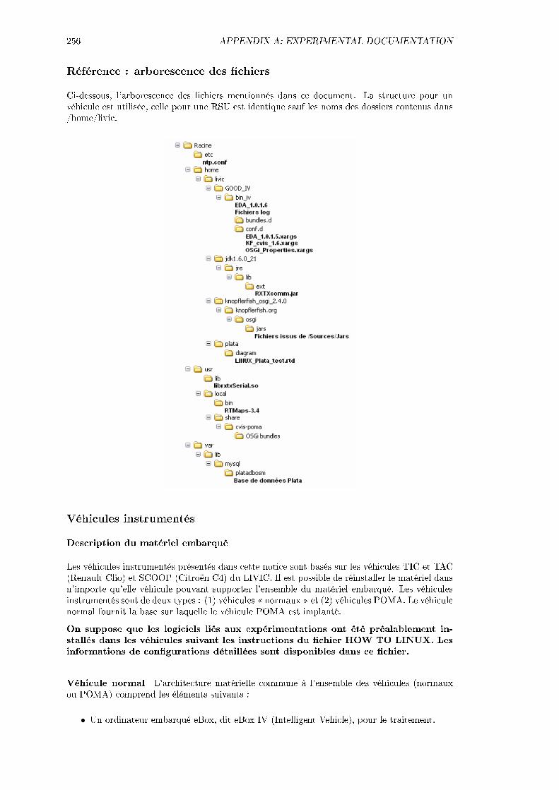
256 APPENDIX A: EXPERIMENTAL DOCUMENTATION

Référence : arborescence des chiers

Ci-dessous, l'arborescence des chiers mentionnés dans ce document. La structure pour unvéhicule est utilisée, celle pour une RSU est identique sauf les noms des dossiers contenus dans/home/livic.

Véhicules instrumentés

Description du matériel embarqué

Les véhicules instrumentés présentés dans cette notice sont basés sur les véhicules TIC et TAC(Renault Clio) et SCOOP (Citroën C4) du LIVIC. Il est possible de réinstaller le matériel dansn'importe qu'elle véhicule pouvant supporter l'ensemble du matériel embarqué. Les véhiculesinstrumentés sont de deux types : (1) véhicules normaux et (2) véhicules POMA. Le véhiculenormal fournit la base sur laquelle le véhicule POMA est implanté.

On suppose que les logiciels liés aux expérimentations ont été préalablement in-stallés dans les véhicules suivant les instructions du chier HOW TO LINUX. Lesinformations de congurations détaillées sont disponibles dans ce chier.

Véhicule normal L'architecture matérielle commune à l'ensemble des véhicules (normauxou POMA) comprend les éléments suivants :

Un ordinateur embarqué eBox, dit eBox IV (Intelligent Vehicle), pour le traitement.

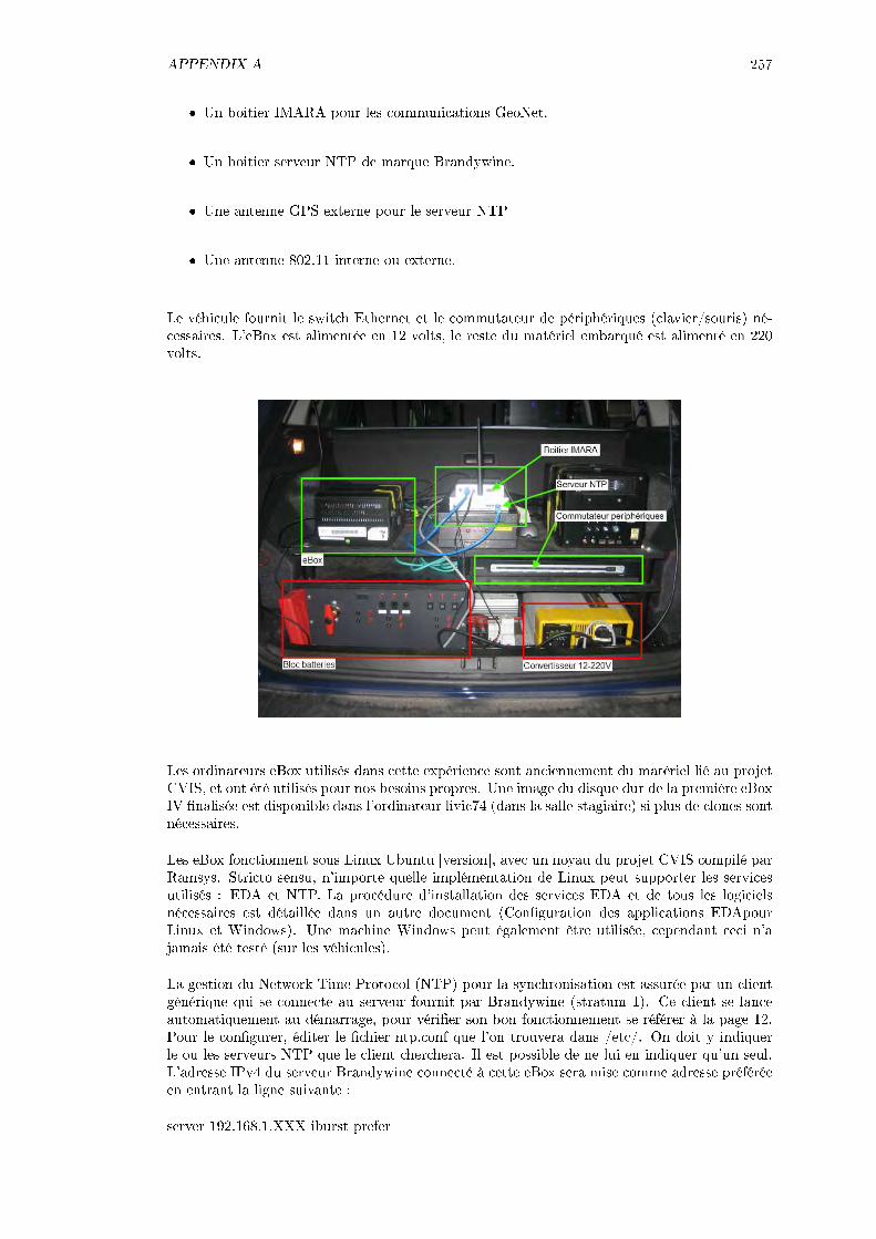
APPENDIX A 257

Un boitier IMARA pour les communications GeoNet.

Un boitier serveur NTP de marque Brandywine.

Une antenne GPS externe pour le serveur NTP

Une antenne 802.11 interne ou externe.

Le véhicule fournit le switch Ethernet et le commutateur de périphériques (clavier/souris) né-cessaires. L'eBox est alimentée en 12 volts, le reste du matériel embarqué est alimenté en 220volts.

Les ordinateurs eBox utilisés dans cette expérience sont anciennement du matériel lié au projetCVIS, et ont été utilisés pour nos besoins propres. Une image du disque dur de la première eBoxIV nalisée est disponible dans l'ordinateur livic74 (dans la salle stagiaire) si plus de clones sontnécessaires.

Les eBox fonctionnent sous Linux Ubuntu [version], avec un noyau du projet CVIS compilé parRamsys. Stricto sensu, n'importe quelle implémentation de Linux peut supporter les servicesutilisés : EDA et NTP. La procédure d'installation des services EDA et de tous les logicielsnécessaires est détaillée dans un autre document (Conguration des applications EDApourLinux et Windows). Une machine Windows peut également être utilisée, cependant ceci n'ajamais été testé (sur les véhicules).

La gestion du Network Time Protocol (NTP) pour la synchronisation est assurée par un clientgénérique qui se connecte au serveur fournit par Brandywine (stratum 1). Ce client se lanceautomatiquement au démarrage, pour vérier son bon fonctionnement se référer à la page 12.Pour le congurer, éditer le chier ntp.conf que l'on trouvera dans /etc/. On doit y indiquerle ou les serveurs NTP que le client cherchera. Il est possible de ne lui en indiquer qu'un seul.L'adresse IPv4 du serveur Brandywine connecté à cette eBox sera mise comme adresse préféréeen entrant la ligne suivante :

server 192.168.1.XXX iburst prefer

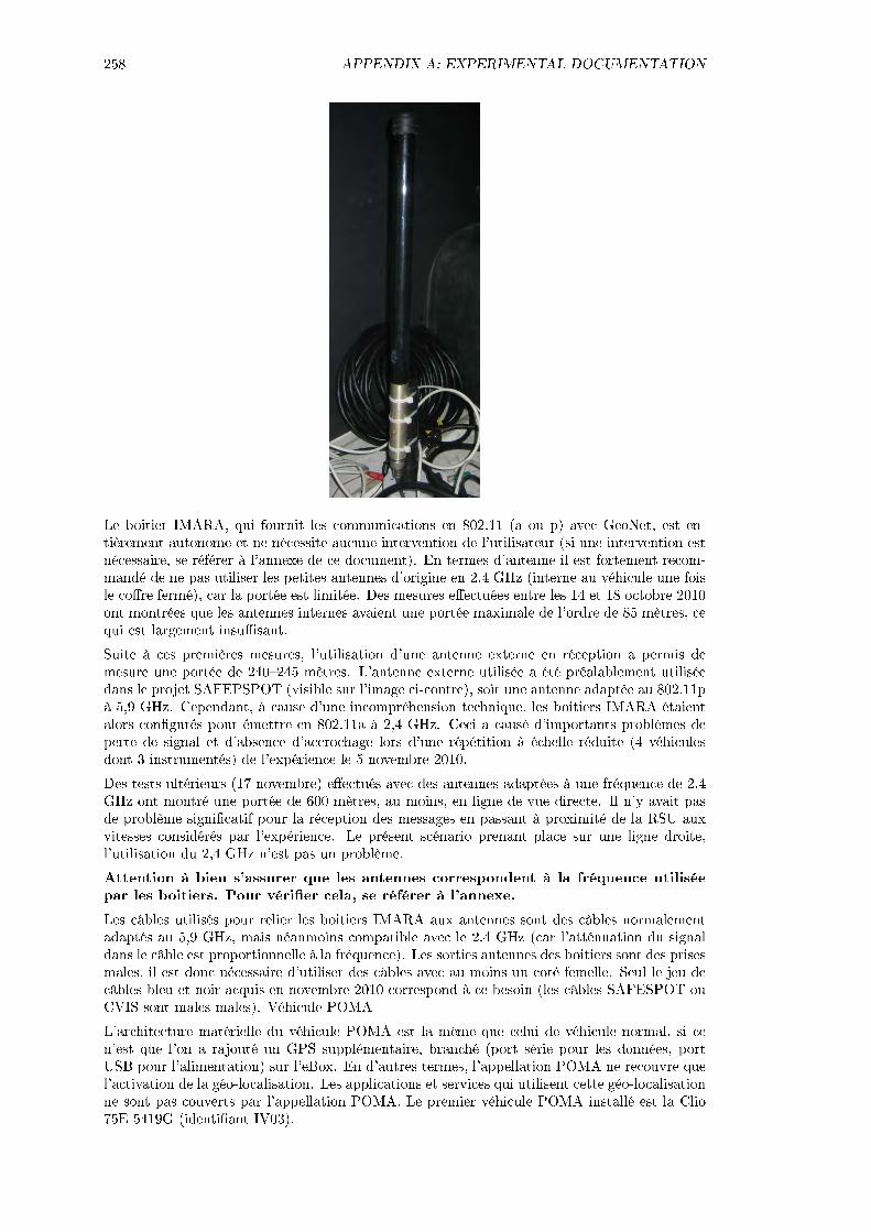
258 APPENDIX A: EXPERIMENTAL DOCUMENTATION

Le boitier IMARA, qui fournit les communications en 802.11 (a ou p) avec GeoNet, est en-tièrement autonome et ne nécessite aucune intervention de l'utilisateur (si une intervention estnécessaire, se référer à l'annexe de ce document). En termes d'antenne il est fortement recom-mandé de ne pas utiliser les petites antennes d'origine en 2.4 GHz (interne au véhicule une foisle core fermé), car la portée est limitée. Des mesures eectuées entre les 14 et 18 octobre 2010ont montrées que les antennes internes avaient une portée maximale de l'ordre de 85 mètres, cequi est largement insusant.

Suite à ces premières mesures, l'utilisation d'une antenne externe en réception a permis demesure une portée de 240245 mètres. L'antenne externe utilisée a été préalablement utiliséedans le projet SAFEPSPOT (visible sur l'image ci-contre), soit une antenne adaptée au 802.11pà 5,9 GHz. Cependant, à cause d'une incompréhension technique, les boitiers IMARA étaientalors congurés pour émettre en 802.11a à 2,4 GHz. Ceci a causé d'importants problèmes deperte de signal et d'absence d'accrochage lors d'une répétition à échelle réduite (4 véhiculesdont 3 instrumentés) de l'expérience le 5 novembre 2010.

Des tests ultérieurs (17 novembre) eectués avec des antennes adaptées à une fréquence de 2.4GHz ont montré une portée de 600 mètres, au moins, en ligne de vue directe. Il n'y avait pasde problème signicatif pour la réception des messages en passant à proximité de la RSU auxvitesses considérés par l'expérience. Le présent scénario prenant place sur une ligne droite,l'utilisation du 2,4 GHz n'est pas un problème.

Attention à bien s'assurer que les antennes correspondent à la fréquence utiliséepar les boitiers. Pour vérier cela, se référer à l'annexe.

Les câbles utilisés pour relier les boitiers IMARA aux antennes sont des câbles normalementadaptés au 5,9 GHz, mais néanmoins compatible avec le 2.4 GHz (car l'atténuation du signaldans le câble est proportionnelle à la fréquence). Les sorties antennes des boitiers sont des prisesmales, il est donc nécessaire d'utiliser des câbles avec au moins un coté femelle. Seul le jeu decâbles bleu et noir acquis en novembre 2010 correspond à ce besoin (les câbles SAFESPOT ouCVIS sont males-males). Véhicule POMA

L'architecture matérielle du véhicule POMA est la même que celui de véhicule normal, si cen'est que l'on a rajouté un GPS supplémentaire, branché (port série pour les données, portUSB pour l'alimentation) sur l'eBox. En d'autres termes, l'appellation POMA ne recouvre quel'activation de la géo-localisation. Les applications et services qui utilisent cette géo-localisationne sont pas couverts par l'appellation POMA. Le premier véhicule POMA installé est la Clio75E 5419G (identiant IV03).

APPENDIX A 259

Comparé à l'architecture normale, l'eBox du véhicule POMA dispose de RTMaps, dont le butest de transmettre au service SpeedAlert d'EDA la position mesurée par le GPS. Les détails dulancement de RTMaps sont décris dans la section suivante.

Conguration des applications EDA

Les chiers de conguration des eBoxes IV se trouvent dans le dossier /home/livic/GOOD_IV-/bin_iv/conf.d. Si la procédure d'installation décrite dans le document HOW TO LINUX estbien suivie, l'eBox est normalement congurée. On rappelle toutefois les points importants ici.

Le chier EDA_1.0.1.5.xargs contient les paramètres les plus importants :

L'identiant unique du véhicule (Dorg.cvisproject.cint.eda.host.identier)

L'adresse du groupe de multicasting auquel les véhicules doivent adhérer, et qui doit êtreréglée dans tous les récepteurs comme l'émetteur (Dorg.cvisproject.cint.eda.comm.multicastAddr)

Les bundles des services souhaités doivent bien être installés et lancés, ce qui revient às'assurer que les lignes suivantes ne sont pas commentées :

install le:./bundles.d/org.cvisproject.cint.eda.service.breakalert.iv-1.0.1.6.jar

start le:./bundles.d/org.cvisproject.cint.eda.service.breakalert.iv-1.0.1.6.jar

Si POMA :

install le:./bundles.d/org.cvisproject.cint.eda.service.speedalert.iv-1.0.1.6.jar

start le:./bundles.d/org.cvisproject.cint.eda.service.speedalert.iv-1.0.1.6.jar

Attention à bien s'assurer que chaque véhicule a un identiant unique au niveaudu paramètre Dorg.cvisproject.cint.eda.host.identier

Arborescence locale :

Procédure de mise en route

On va maintenant décrire la marche à suivre pour mettre en route les véhicules instrumentésnormaux et modiés POMA. Cette section est organisée linéairement dans l'ordre recommandéde la mise en route du matériel et des logiciels.

260 APPENDIX A: EXPERIMENTAL DOCUMENTATION

Alimentation Les besoins en alimentation sont d'une prise 12 volt pour l'eBox et de prises220 volt pour les boitiers IMARA et NTP Brandywine. L'alimentation des écrans et autresmatériels embarqués est déjà assurée au niveau du véhicule et ne nécessite aucun câblage ouinstallation supplémentaire.

Les prises 220 volts doivent être branchées à la multiprise connectée sur le convertisseur12-220 volts.

La prise 12 volt de l'eBox doit être connectée sur les connecteurs plastiques du rack,comme montré sur l'image ci-dessous.

Le GPS de l'eBox POMA est alimenté en USB par l'ordinateur lui-même.

Attention à bien débrancher l'USB tant que l'eBox n'est pas complètement lancée,car le GPS peut être abusivement interprété comme un périphérique d'interface.

La procédure suivante doit être suivie pour alimenter l'ensemble :

Tourner le ou les commutateurs généraux sur les positions on (horizontale).

Mettre les deux boutons de batteries 12 V sur on, voyants allumés.

Le convertisseur 12-220V doit être alimenté, l'allumé s'il ne l'était pas déjà.

Le C4 possède deux commutateurs. Le commutateur placé le plus à gauche permet l'alimentationdes écrans dans l'habitacle indépendamment du reste du circuit. Les deux boutons les plus àgauche seulement doivent êtres positionnés sur on.

Vérier le bon lancement des boitiers IMARA et NTP, qui s'allument automatiquement dèsqu'ils sont alimentés. L'eBox nécessite une intervention manuelle sur le bouton de démarrage(sur la face arrière) pour se lancer.

APPENDIX A 261

Alimentation pour essais statiques Pour des essais statiques dans le garage ou à proximitéimmédiate d'un accès au secteur, il est recommandé de fonctionner ainsi :

Débrancher la multiprise du convertisseur 12-220V et la brancher sur une prise secteur.

Mettre le convertisseur en position o.

Mettre les batteries en ligne (commutateurs plus boutons) mais brancher un chargeurcomme sur l'image ci-dessous.

Attention, les batteries du C4 ne sont pas rechargées par l'alternateur du moteurthermique comme sur les Clios, il faut donc :

1. Recharger le véhicule après utilisation.

2. S'assurer qu'on alimente et démarre les systèmes du C4 en dernier.

Démarrage de l'eBox Attention, certaines eBox peuvent avoir un oppy disk fail ou uneerreur CMOS. Appuyez sur F1 et continuer d'opérer normalement.

Une fois Linux lancé, le premier bureau est bugé (délement en boucle), passer sur le secondbureau en tapant Ctrl + Alt + F2.

Le compte utilisateur est livic, mot de passe : cvis. Il est fortement recommandé de passeren super-utilisateur avec le commande sudo s (le mot de passe peut être redemandé, c'est lemême que ci-dessus).

Entrer la commande startx pour lancer l'interface graphique Xfce. A ce stade, sur un IV POMA,le GPS peut être branché.

Attention à bien vérier que le switch de commutation de périphériques est correctementréglé : il n'active pas nécessairement par défaut l'entrée qui est branchée. Les câbles dans lesvéhicules sont marqués pour retrouver facilement quel câble correspond à quelle entrée.

Vérication de la connectivité 802.11/IPv6

Ouvrir un nouveau terminal et y taper ifcong. Si le réseau est bien actif et que le boitierIMARA fonctionne bien on devrait obtenir un résultat comme ci-dessous :

262 APPENDIX A: EXPERIMENTAL DOCUMENTATION

On peut y noter une adresse IPv4 dans la gamme 192.168.1.XXX. Cette adresse est xe, at-tribuée par défaut au lancement et est locale à chaque véhicule. Deux eBox peuvent avoirla même adresse tant qu'elles ne sont pas mise en réseau. On peut modier cette adresse(non recommandé) en modiant le chier /etc/network/interfaces (utilisation de l'éditeur nanorecommandé, ne pas oublier de relancer l'interface après).

On peut y noter également deux lignes concernant des adresses IPv6. Si une seule ligne estvisible, l'eBox n'a pas obtenu d'adresse IPv6. Pour régler ce problème on peut :

Taper la commande ifcong eth0 down puis ifcong eth0 up.

Attendre quelques minutes que le boitier IMARA soit proprement initialisé.

Attention (1), le nom de l'interface peut être eth0 ou eth1 en fonction des machines. Unvéhicule sera généralement en eth1. Cela n'impacte pas le fonctionnement normal, juste lescommandes à taper en cas de problème.

Toujours vérier en tapant à nouveau ifcong. Se référer à la page 32 pour des moyens plussophistiqués de vérier le bon fonctionnement de la connectivité.

Attention (2), l'un des boitiers IMARA n'est pas tout à fait conguré au démarrage commeles autres. Le DHCP n'y est pas désactivé, ce qui signie que le boitier va prendre plus detemps pour se lancer, attendant le time-out de sa recherche de DHCP. Une fois cette étapepassée, le boitier fonctionne de manière autonome comme les autres.

Attention (3), il est courant que les boitiers IMARA notent des erreurs au démarrage, dues àl'arrêt par coupure de l'alimentation. Les boitiers eectuent une vérication de leur disque etse relancent avant de fonctionner normalement par la suite.

Vérication du NTP Normalement, le client NTP se met en route automatique lors dulancement de Linux et se connecte immédiatement au serveur Brandywine si le chier /etc/-ntp.conf contient la bonne adresse et la connectivité réseau est active.

Attention, certaines eBox peuvent acher une date en janvier 2003 peut de temps après leurlancement. Le NTP corrige cette erreur après quelques minutes.

Pour vérier que le NTP fonctionne bien :

S'assurer que la LED Valid Time est bien allumée (elle se trouve sous le connecteur del'antenne). Si cette LED n'est pas allumée, le serveur n'a pas encore réussit à acquérir unebase de temps stable. Le serveur peut fonctionner en intérieur, mais il est recommandéde se placer à l'extérieur pour acquérir une bonne base plus rapidement.

Ouvrir un terminal, puis taper ntpq. Taper ensuite associations puis peers. On doitobtenir les résultats suivants si tout fonctionne correctement (image ci-dessous). Taperexit pour quitter le mode ntpq.

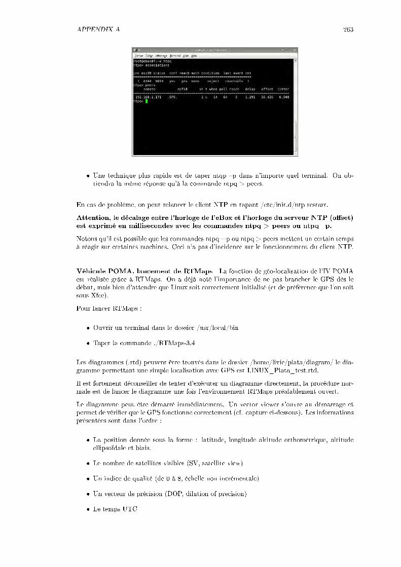
APPENDIX A 263

Une technique plus rapide est de taper ntqp p dans n'importe quel terminal. On ob-tiendra la même réponse qu'à la commande ntpq > peers.

En cas de problème, on peut relancer le client NTP en tapant /etc/init.d/ntp restart.

Attention, le décalage entre l'horloge de l'eBox et l'horloge du serveur NTP (oset)est exprimé en millisecondes avec les commandes ntpq > peers ou ntpq p.

Notons qu'il est possible que les commandes ntpq p ou ntpq > peers mettent un certain tempsà réagir sur certaines machines. Ceci n'a pas d'incidence sur le fonctionnement du client NTP.

Véhicule POMA, lancement de RTMaps La fonction de géo-localisation de l'IV POMAest réalisée grâce à RTMaps. On a déjà noté l'importance de ne pas brancher le GPS dès ledébut, mais bien d'attendre que Linux soit correctement initialisé (et de préférence que l'on soitsous Xfce).

Pour lancer RTMaps :

Ouvrir un terminal dans le dossier /usr/local/bin

Taper la commande ./RTMaps-3.4

Les diagrammes (.rtd) peuvent être trouvés dans le dossier /home/livic/plata/diagram/ le dia-gramme permettant une simple localisation avec GPS est LINUX_Plata_test.rtd.

Il est fortement déconseiller de tenter d'exécuter un diagramme directement, la procédure nor-male est de lancer le diagramme une fois l'environnement RTMaps préalablement ouvert.

Le diagramme peut être démarré immédiatement. Un vector viewer s'ouvre au démarrage etpermet de vérier que le GPS fonctionne correctement (cf. capture ci-dessous). Les informationsprésentées sont dans l'ordre :

La position donnée sous la forme : latitude, longitude altitude orthométrique, altitudeellipsoïdale et biais.

Le nombre de satellites visibles (SV, satellite view)

Un indice de qualité (de 0 à 8, échelle non incrémentale)

Un vecteur de précision (DOP, dilution of precision)

Le temps UTC

264 APPENDIX A: EXPERIMENTAL DOCUMENTATION

Il est conseillé d'utiliser un bureau diérent pour RTMaps, an de ne pas encombrer l'écran.Xfce permet d'utiliser jusqu'à quatre bureaux accessibles en faisant glisser les fenêtres, par lamolette de la souris ou via le panneau de lancement rapide.

Le ux GPS peut être enregistré en connectant un composant recorder à l'une des sorties (enfonction du formatage que l'on recherche). Ne pas oublier de spécier le chemin d'accès pourle chier d'enregistrement, sinon il se placera dans /usr/local/bin par défaut.

Véhicule POMA, lancement de MySQL MySQL est nécessaire pour le service SpeedAlert(qui utilise également RTMaps). Les véhicules POMA sont aussi équipés d'un serveur/clientMySQL Linux qui doit être démarrée avant les services.

Le serveur MySQL démarre automatiquement avec Linux, mais aucune base de donnée n'estparamétrée pour être utilisée par défaut. Pour indiquer la bonne base de donnée au serveurMySQL :

Ouvrir un terminal dans n'importe quel dossier

Taper la commande mysql u root p et indiquer le mot de passe livic

Taper use platadbosm

Taper status, le nom de la banque de donnée active doit être visible sur la seconde ligne(cf. capture ci-dessous)

Lancement des services EDA Attention, si les bundles ont été changés, il estnécessaire de supprimer le dossier /home/livic/eda pour s'assurer que les nouveauxbundles sont bien installés et pris en compte lors du lancement d'EDA.

Si tout est correctement conguré, le lancement d'EDA et des services est simple :

Ouvrir un terminal dans le dossier /home/livic/GOOD_IV/bin_iv

APPENDIX A 265

Taper ./EDA_1.0.1.6

Une fois l'application lancée, cliquez deux fois sur le panneau dans le coin inférieur droitpour activer les services (cf. capture).

Une fois lancée, l'application n'a plus besoin d'aucune intervention humaine. Lorsqu'un messageest reçu et correctement interprété par l'application, un panneau de signalisation danger triangulaire apparait dans la moitié droite de l'interface.

Les applications liés aux véhicules POMA (service SpeedAlert) ajoutent des objets supplé-mentaires dans l'interface. La limite de vitesse courante est achée dans la partie gauche etune alerte de dépassement de cette limite s'ache dans la partie droite si c'est le cas. Cetachage peut entrer en conit avec celui du service BreakAlert ; dans ce cas, l'un des pan-neaux est aché en petit en dessous de l'autre. Il est recommandé pour cette raison de ne pasactivé SpeedAlert lors d'essai avec une le de véhicule ou de les réaliser sur une route dont lalimitation de vitesse native est supérieure à la vitesse maximale obtenue dans l'expérience.

Attention, à l'arrêt le service SpeedAlert peut enregistrer une vitesse non-nulle à cause des er-reurs de positionnement GPS. Cela entrainera l'apparition intempestive d'une alerte de dépassede vitesse. Ces alertes n'ont pas d'incidence sur le bon fonctionnement du service.

Attention, de nombreuses alertes sont visibles dans le terminal indiquant qu'une applicationPOMA ne peut pas se connecter au localhost. Ignorer ces alertes.

Logs

Les logs des applications sont stockés directement dans le dossier /home/livic/GOOD_IV/bin_ivdans des chiers .log. Les chiers s'accumulant après un certain temps (un nouveau chier estcréé à chaque lancement d'EDA), il est recommandé de les purger de temps à autres.

Les applications écrivent toutes dans un unique chier de log dont la structure a été normaliséean de pouvoir être aisément exploitable avec des logiciels comme Excel ou Matlab. Attention,si des bundles datant d'avant le 22 novembre 2010 sont utilisés, les logs ne seront pas normalisés: ils seront plus facile à lire pour un humain mais plus complexe à trier pour une exploitationrapide, comprenant notamment beaucoup de verbose qui peut poser problème à une applicationcomme Matlab. Pour les bundles postérieurs au 22 novembre, la structure suivante a été adoptée:

16:05:33.985;;spy;IV-03;spy6;48.78521666666667;2.099683333333333;29;

11:05:47.097;;ba;RSU;breakAlert1;11:05:47.093;

Le log se présente sous le format d'une feuille CSV (character-separated value) avec une sépara-tion par points-virgules. Les premières colonnes contiennent toujours les mêmes valeurs an depermettre de trier facilement le chier, mais les colonnes de données supplémentaires peuventvarier en nombre. Les colonnes initiales sont :

266 APPENDIX A: EXPERIMENTAL DOCUMENTATION

Le timestamp donné juste sous la forme de l'heure, à la milliseconde près. La date del'enregistrement peut être trouvée dans le nom du chier plutôt que dans le log en lui-même.

Une colonne vide qui permet de maintenir l'alignement des colonnes. Cette colonne est(rarement) utilisée pour une variation spécique de l'application.

Un identiant du type d'information contenu dans la ligne. Les identiants possibles sont:

ba : pour un log relevant du service BreakAlert (prise en compte du signal provenantdu cône-détecteur)

spy : pour un log relevant du service Spy (service assurant un enregistrement et unetransmission des informations GPS une fois par seconde).

MulticastTo ou MulticastFrom : pour un log relevant de l'envoi ou de la réceptiond'un message multicasting

UnicastTo ou UnicastFrom : pour un log relevant de l'envoi ou de la réception d'unmessage unicasting

L'identiant du l'acteur (véhicule ou RSU) à l'origine de l'information de la ligne

L'identiant de l'événement dans le service d'origine, que l'on peut utiliser pour retracerpar exemple l'identiant particulier d'un message.

Viennent ensuite les colonnes réservées aux données, par exemple dans le cas d'un messageBrakeAlert MulticastFrom l'heure à laquelle le signal du cône-détecteur a été reçu, ou bienencore dans le cas d'un message spy la latitude, la longitude et la vitesse (telle que calculée àpartir du GPS).

Attention, les messages de type xTo ont une structure légèrement diérente : il n'y a pasd'identiant de l'expéditeur ou du service concerné ; après l'identiant de type on trouvel'adresse cible (précise dans le cas d'un unicast ou le groupe dans le cas d'un multicast) etpuis le port utilisé pou émettre le message.

Les logs RTMaps, s'ils sont présents, sont stockés dans les dossiers spéciés par l'utilisateur ou,par défaut, dans /usr/local/bin.

Procédure d'arrêt

Logiciels Il est recommandé d'arrêter proprement les logiciels de la manière suivante :

EDA est arrêté en sélectionnant le terminal hôte et en tapant Ctrl + c, il est déconseillerde fermer le terminal comme on procéderait pour une application DOS sous Windows.

RTMaps est arrêté comme sous Windows, en cliquant sur la croix ou en quittant dans lemenu principal ; le terminal qui l'hébergeait peut ensuite être fermé sans soucis.

Le client NTP ou MySQL n'ont pas besoin d'être arrêté. Pour éteindre l'eBox, clique-droitn'importe où dans un bureau, aller sur l'onglet quitter du menu déroulant et sélectionneréteindre.

Matériel La procédure d'arrêt recommandée est la suivante :

1. Arrêt de l'eBox.

2. Arrêt du convertisseur 12-220V, induit l'arrêt du serveur NTP Brandywine et du boitierIMARA.

3. Mettre les deux boutons des batteries sur o.

4. Tourner le ou les commutateurs en position o (verticale).

Ne pas oublier de mettre en charge les batteries du C4.

APPENDIX A 267

Road side unit

Description du matériel

La road side unit (RSU) se compose du même matériel que les véhicules, à l'exception du ré-cepteur sans-ls lié au cône détecteur. L'eBox, le serveur NTP Brandywine et le boitier IMARAsont identiques à ceux utilisés dans les véhicules, avec des diérences logicielles seulement. Lerécepteur du cône-détecteur est branché (port série) sur l'eBox via un câble RS232 modié pourtransformer la sortie 12 volts en signal compréhensible sur le ring RS232.

En rouge : le matériel d'alimentation ; en vert : le matériel de la RSU

Conguration des applications EDA

Les chiers de conguration de l'eBox RSU se trouvent dans le dossier /home/livic/GOOD_RSU-/bin_rsu/conf.d. Si la procédure d'installation décrite dans le document HOW TO LINUX estbien suivie, l'eBox est normalement congurée. On rappelle toutefois les points importants ici.Le chier EDA_1.0.1.5.xargs contient les paramètres les plus importants :

L'identiant unique de la RSU (Dorg.cvisproject.cint.eda.host.identier)

L'adresse du groupe de multicasting (Dorg.cvisproject.cint.eda.comm.multicastAddr), quiest réglée à 02::1 par défaut.

Le port série sur lequel l'application écoutera pour le signal du cône-détecteur (Dorg.cvisproject.cint.eda.breakalert.portcom),qui est réglé sur /dev/ttys0 par défaut (équivalent à COM1 sous Windows).

Les bundles des services souhaités doivent bien être installés et lancés, ce qui revient às'assurer que les lignes suivantes ne sont pas commentées :

install le:./bundles.d/org.cvisproject.cint.eda.service.breakalert.rsu-1.0.1.6.jar

start le:./bundles.d/org.cvisproject.cint.eda.service.breakalert.rsu-1.0.1.6.jar

Rappel : le port série 1 (/dev/ttys0) est celui qui est placé directement sous le port Ethernetsur les eBoxes.

Pour le service SpeedAlert, il faut simplement s'assurer que le port sur lequel le récepteur ducône-détecteur dédié est bien réglé (/dev/ttys1 par défaut) et que le service est bien actif, avecla même procédure que ci-dessus.

268 APPENDIX A: EXPERIMENTAL DOCUMENTATION

Procédure de mise en route

On va maintenant décrire la marche à suivre pour mettre en route la RSU. Cette section estorganisée linéairement dans l'ordre recommandé de la mise en route du matériel et des logiciels.

Alimentation Les besoins en alimentation sont les mêmes que pour le matériel embarquédans les véhicules : une prise 12 volt pour l'eBox et de prises 220 volt pour les boitiers IMARA etNTP Brandywine. L'alimentation des écrans et autres matériels (commutateur périphériques)est assurer via une multiprise commune qui peut être connectée directement sur le secteur, surun groupe électrogène ou à un convertisseur 12-220 volt, lui aussi présent sur le rack.

La procédure suivante doit être suivie pour alimenter l'ensemble :

Abaisser le commutateur de la batterie de manière à ce que le cylindre métallique ne soitplus visible (le commutateur en position ouverte est montré ci-après).

Connecter la multiprise au secteur ou au groupe électrogène (après avoir préalablementdémarré celui-ci). Eventuellement utiliser le convertisseur 12-220V.

Le boitier IMARA, le commutateur de périphériques et le serveur NTP s'allument dès qu'ilssont alimentés, l'eBox doit être allumée manuellement.

Démarrage de l'eBox Attention, certaines eBox peuvent avoir un oppy disk fail ou uneerreur CMOS. Appuyez sur F1 et continuer d'opérer normalement.

Le compte utilisateur est livic, mot de passe : cvis. Il est fortement recommandé de passeren super-utilisateur avec le commande sudo s (le mot de passe peut être redemandé, c'est lemême qui ci-dessus).

Entrer la commande startx pour lancer l'interface graphique Xfce.

Connectivité & NTP Pour la vérication de la connectivité et du bon fonction-nement du NTP se référer aux pages concernant les véhicules, respectivement page11 et page 12.

Lancement des services EDA Attention, si les bundles ont été changés, il est nécessairede supprimer le dossier /home/livic/eda pour s'assurer que les nouveaux bundles sont bieninstallés et pris en compte lors du lancement d'EDA.

Si tout est correctement conguré, le lancement d'EDA et des services est simple :

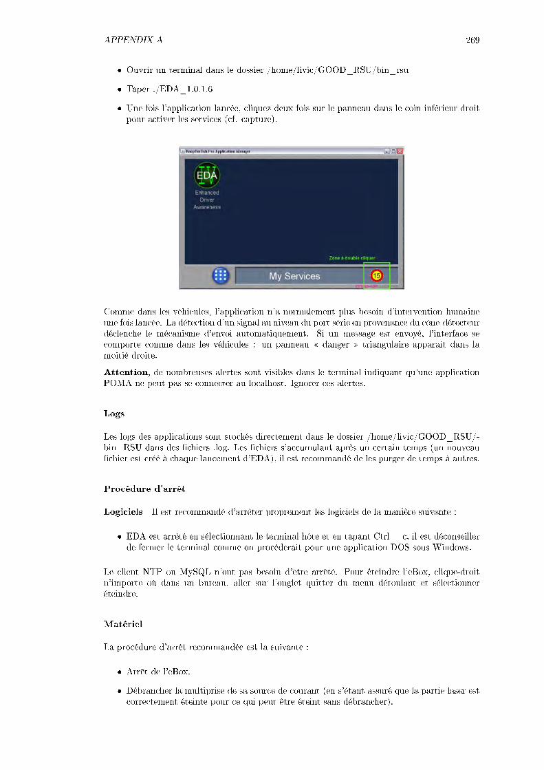
APPENDIX A 269

Ouvrir un terminal dans le dossier /home/livic/GOOD_RSU/bin_rsu

Taper ./EDA_1.0.1.6

Une fois l'application lancée, cliquez deux fois sur le panneau dans le coin inférieur droitpour activer les services (cf. capture).

Comme dans les véhicules, l'application n'a normalement plus besoin d'intervention humaineune fois lancée. La détection d'un signal au niveau du port série en provenance du cône-détecteurdéclenche le mécanisme d'envoi automatiquement. Si un message est envoyé, l'interface secomporte comme dans les véhicules : un panneau danger triangulaire apparait dans lamoitié droite.

Attention, de nombreuses alertes sont visibles dans le terminal indiquant qu'une applicationPOMA ne peut pas se connecter au localhost. Ignorer ces alertes.

Logs

Les logs des applications sont stockés directement dans le dossier /home/livic/GOOD_RSU/-bin_RSU dans des chiers .log. Les chiers s'accumulant après un certain temps (un nouveauchier est créé à chaque lancement d'EDA), il est recommandé de les purger de temps à autres.

Procédure d'arrêt

Logiciels Il est recommandé d'arrêter proprement les logiciels de la manière suivante :

EDA est arrêté en sélectionnant le terminal hôte et en tapant Ctrl + c, il est déconseillerde fermer le terminal comme on procéderait pour une application DOS sous Windows.

Le client NTP ou MySQL n'ont pas besoin d'être arrêté. Pour éteindre l'eBox, clique-droitn'importe où dans un bureau, aller sur l'onglet quitter du menu déroulant et sélectionneréteindre.

Matériel

La procédure d'arrêt recommandée est la suivante :

Arrêt de l'eBox.

Débrancher la multiprise de sa source de courant (en s'étant assuré que la partie laser estcorrectement éteinte pour ce qui peut être éteint sans débrancher).

270 APPENDIX A: EXPERIMENTAL DOCUMENTATION

Relever le commutateur de la batterie de manière à ce que le cylindre métallique soitvisible.

Il est recommandé de remettre en charge régulièrement la batterie utilisée par le bloc RSU-Laser. Le même type de chargeur que pour les véhicules (12 volts, 10 ampères) doit être utilisé; plusieurs type de connecteurs diérents sont disponibles sur les chargeurs du LIVIC en fonctionde la batterie montée avec la RSU.

Le cône-détecteur doit aussi régulièrement être rechargé. Il n'est pas recommandé d'utiliser lesmêmes chargeurs que pour les véhicules ou la RSU, mais plutôt un chargeur plus petit (900mA, image ci-dessous). Chaque cône dispose de deux connecteurs placés sous le commutateuron/o pour accès à la batterie.

Ne pas oublier de mettre en charge les batteries du C4.

Unité laser LUX

Description du matériel

En rouge : le matériel d'alimentation ; en jaune : le matériel de l'unité laser

APPENDIX A 271

L'unité laser telle que mise en ÷uvre dans cette notice est partiellement liée à la RSU, cependantla RSU et l'unité laser n'ont aucun besoin d'être liées : elles peuvent fonctionner de manièrecomplètement indépendante. L'unité laser se compose d'un ordinateur embarqué de marqueXpc, sous Windows XP, du LUX Fusion System IBEO (2 capteurs + une ECU). Le matérielpartagé avec la RSU est le serveur NTP Brandywine, le switch Ethernet et l'alimentation (12 et220 volts). Les deux capteurs du LUX sont montés sur une barre d'acier an d'être positionnerà plat correctement. La barre peut être montée sur un trépied (comme sur l'image ci-avant)ou sur tout autre type de support. L'écart entre les deux capteurs ou l'orientation de chacunpeuvent être modiés, mais ceci nécessitera alors de remesurer ces variables.

Conguration des applications

Les logiciels et applications utilisés dans l'unité laser LUX ne nécessitent pas de congurationspécique qui ne soit pas explicitée dans les paragraphes ci-après.

Procédure de mise en route

On va maintenant décrire la marche à suivre pour mettre en route l'unité laser LUX. Cettesection est organisée linéairement dans l'ordre recommandé de la mise en route du matériel etdes logiciels.

Alimentation Les besoins en alimentation sont d'une prise 12 volt pour le système LUX etde 220 volts pour le reste du matériel. Le LUX est alimenté via l'ECU, qui doit être connectéedirectement sur la batterie ou peut être relié au commutateur général du rack RSUunité laser.Pour le matériel nécessitant du 220 volts, la multiprise générale de la RSUunité laser comportetoutes les connexions nécessaires (ordinateur, écran, etc.). Suivre la même procédure que page21 pour alimenter l'ensemble de l'unité laser.

Attention, bien s'assurer que les deux télémètres lasers sont connectés à l'ECU avant del'alimenter.

Démarrage du PC L'ordinateur se démarre comme tout PCWindows. Le compte d'utilisateurest livic et il n'y a pas de mot de passe.

Lancement du client NTP Contrairement à un système Linux, le client NTP peut ne passe lancer automatiquement lors du démarrage de la machine Windows. Si on doit le lancer,cliquer sur l'icône NTP Time Server Monitor présente sur le bureau (dans la capture ci-dessous,le client NTP est déjà conguré pour démarrer automatiquement, ce qui est réglage dans lapartie Service conguration à droite).

272 APPENDIX A: EXPERIMENTAL DOCUMENTATION

Le client est conguré pour utiliser le même serveur Brandywine que la RSU (soit 192.168.1.163),mais peut être modié pour utiliser son propre serveur. Pour cela, cliquer sur l'onglet NTPConguration File et modier le chier en dessous de la ligne # Positioning PC comme sur lacapture ci-dessous. La ligne non commentée (sans # devant) est active ; il est possible d'avoirplusieurs serveurs listés, le client essayera de se connecter à ces serveurs et sélectionnera celuiqui fonctionne le mieux. Lister un serveur non accessible n'est pas un problème, sauf si onsouhaite limiter les interrogations du client vers l'adresse de ce serveur. Ecrire prefer aprèsl'adresse IP d'un serveur permet de le priviliger par rapport aux autres.

Pour vérier que le serveur fonctionne, aller sur l'onglet NTP Status. L'adresse du serveur doitêtre visible, avec divers informations concernant le statut du client et le décalage entre les deuxhorloges. Si le client a terminé son processus d'initialisation, l'ensemble de la ligne doit êtresurligné en vert (cf. capture ci-dessous).

Vérication du bon fonctionnement du système LUX Le système Ibeo LUX s'initialiseimmédiatement une fois alimenté. Pour vérier qu'il fonctionne bien, plusieurs démarches sontpossibles.

En premier lieu, une vérication visuelle de l'état des LED sur le dos de l'ECU est nécessaire.Si tout fonctionne bien, les LED de l'alimentation (verte) et des deux câbles reliant l'ECU auxcapteurs (oranges) doivent être allumées.

APPENDIX A 273

En second lieu, on doit vérier que les données sont bien transmisses sur le réseau et queles réglages du système (hardware comme software) sont corrects. Pour vérier que le systèmeproduit des données, on peut utiliser le logiciel fournit par Ibeo ILV-Basic. On peut le démarrervia le menu démarrer / ILV-Basic 1.7.1 / ILV-Basic ou en allant dans le dossier C:\Documentsand Settings\livic\Bureau\Demmel\ et en cliquant sur l'icône appropriée. Une fois le logiciellancé, entrer l'adresse IP de l'ECU dans la fenêtre en haut à droite et cliquer sur connect.

[CAPTURE DE LA BARRE DU MENU]

Si l'ECU et les capteurs sont actifs, la carte des données envoyées par les capteurs devraitapparaitre, remplaçant l'image de fond. Si les positions et orientations des deux capteurs sontbien réglés, la carte doit fournir une vue cohérente de l'environnement.

[CAPTURE DU LOGICEL ACTIF]

(expliquer comment régler le logiciel)

Lancement de RTMaps La fonction de RTMaps est d'enregistré les données produites parle système LUX. Pour lancer RTMaps, aller à menu démarrer / Intempora / RTMaps 3.2 /RTMaps Studio. Plusieurs diagrammes sont utilisables. Il est fortement déconseiller de tenterd'exécuter un diagramme directement, la procédure normale est de lancer le diagramme unefois l'environnement RTMaps préalablement ouvert.

Un premier diagramme préconguré Ethernet_raw_recorder.rtd peut être trouvé dans le dossierR:\Demmel. Il contient un composant réalisé par Intempora pour eectuer une connexion avecl'ECU du système LUX et sauvegarder les données brutes et traitées issues des lasers. Il est re-commandé de choisir un chemin d'accès personnalisé pour l'enregistrement des données avec lecomposant recorder (pour ce, clique droit sur le composant, propriétés puis modier la premièrepropriété).

Le second diagramme préconguré ECU_decoder_recorder.rtd peut être trouvé dans le mêmedossier. Il s'agit d'une version plus sophistiquée du premier diagramme, avec plusieurs com-posants Intempora en cascade pour se connecter avec l'ECU et décoder les données reçues decelui-ci. Le composant OGS Viewer permet par exemple de visualiser en trois dimensions lenuage de points détectés en direct. Les deux autres composants présents sur l'image (scannerinfo splitter et objects info splitter) permettent de formater correctement certaines informationsdonnées sous forme de string par le premier composant. D'autres composants sont disponiblesdans le package rtmaps_ibeo_ethernet.pck. On peut connecter les sorties de ces composantsà divers recorders pour en enregistrer les sorties selon les besoins.

Les diagrammes doivent être démarrés seulement au moment souhaité lors de l'expérimentation,an de limiter la durée de la collecte des données (et faciliter le travail d'analyse ultérieure).

Procédure d'arrêt

Logiciels L'arrêt de la machine Windows ne présente pas de diculté particulière. Il estrecommandé d'arrêter proprement les logiciels de la manière suivante :

274 APPENDIX A: EXPERIMENTAL DOCUMENTATION

RTMaps est arrêté, après s'être bien assuré que le diagramme ne tourne plus, en cliquantsur la croix ou en quittant dans le menu principal.

Cliquer sur la croix pour quitter le client NTP.

Si l'ILV-Basic est utilisé, cliquer sur la croix comme pour tout autre logiciel.

Le client NTP n'a pas besoin d'être arrêté. On ne doit pas non plus arrêté les logiciels internesà l'ECU LUX, qui sont inaccessibles en temps normal.

Matériel La procédure d'arrêt recommandée est la suivante :

Arrêt du PC Windows

Débrancher la multiprise de sa source de courant (en s'étant assuré que la partie RSU estcorrectement éteinte pour ce qui peut être éteint sans débrancher).

Relever le commutateur de la batterie de manière à ce que le cylindre métallique soitvisible.

Le système LUX ne sera plus alimenté lorsque le commutateur principal est relevé. Il n'y a pasde précaution particulière à prendre avant de l'éteindre.

Outils divers

Vérication de la connectivité Wireshark

Pour pouvoir vérier la connectivité, il est présentement impossible de se connecter directementdans les boitiers IMARA. Cependant, on peut observer les interfaces Ethernet pour vérier queles messages sont bien expédiés par EDA RSU ou reçu dans les véhicules. Cette opération estréalisée avec Wireshark. Pour le lancer, ouvrir un terminal n'importe où et taper wireshark.Une fois le logiciel lancé, cliquez sur le premier bouton à gauche pour obtenir la liste desinterfaces disponibles.

Sélectionner eth0 (ou eth1 en fonction de l'eBox) et cliquer sur capture ; ignorer les messagesd'erreur.

Une liste glissante des paquets échangés sur l'interface apparait alors, par défaut les messagesles plus récents sont en bas. Pour arrêter le délement de la liste, simplement monter la vue demanière à ce que le paquet le plus récent ne soit pas visible. En fonctionnement normal, despaquets liés au NTP et au fonctionnement de GeoNet (router solication, neigbhour advertise-ment, etc.) sont visibles en majorité. Les paquets EDA sont de type UDP (attention, le NTPet l'UDP sont aché dans la même couleur).

[CAPTURE D'UN MESSAGE NORMAL]

En date d'octobre 2010, un problème de fragmentation des paquets existe dans GeoNet. Siun message est fragmenté parce qu'il est trop volumineux, le premier paquet va passer mais lesecond n'apparaitra pas sur l'interface des récepteurs. L'absence de ce paquet (même s'il necontient que quelques octets de données utiles) empêche EDA d'interpréter le message correcte-ment : aucune réaction n'est visible au niveau de l'application. Si ce problème est détecté, lameilleure solution consiste à réduire la taille du message à l'émission pour qu'il rentre dans unseul paquet (environ un kilo-octet au maximum).

APPENDIX A 275

Exemple de fonctionnement anormal due à la fragmentation Dans la capture ci-dessous, on a l'enregistrement des paquets au niveau de la RSU envoyé en unicasting (adresseunique). Le message envoyé par EDA est coupé entre les paquets 27 et 28, le dernier étantréinterprété comme le message entier.

Dans la capture ci-dessous au niveau d'un véhicule, le paquet 82 correspond au paquet 27 ci-dessus (les temps indiqués à la deuxième colonne ne sont pas représentatifs du délai entre laRSU et l'IV). Le détail du paquet est fourni ci-après. On peut remarquer, dans la ligne ensurbrillance, que le drapeau More Fragment est vrai. Sachant que le second paquet attendun'arrive pas, le message ne sera pas interprété par EDA comme valide.

Attention, Wireshark n'est pas installé sur toutes les eBoxes. Pour l'installer, ilfaut se connecter à internet (se référer au document HOW TO LINUX pour laprocédure d'activation d'internet si besoin est) et taper apt-get install wireshark(taper apt-get update est recommandé avant).

Portage d'un service

Il est possible de porter un service EDA RSU dans un véhicule et vice versa sans dicultés, lematériel pour les supporter étant le même. Si on souhaite pouvoir disposer d'une RSU sur unvéhicule, la procédure suivante doit être suivie :

Eectuer une copie du dossier /bin_rsu (il est recommandé d'en purger les logs dans lacopie) sur un support amovible.

Coller ce dossier dans un dossier de son choix dans la machine cible, par exemple dans/GOOD_IV.

Dans /bin_rsu, ouvrir le chier EDA_1.0.1.6 (avec l'éditeur mousepad) et dans /bin_rsu/-conf.d ouvrir les chiers KF_cvis_1.6.xargs et OSGi_Properties.xargs et vérier que leschemins d'accès pointent vers les bon dossiers. Il est possible que les environnementsJava et Knopersh ne soient pas installés exactement au même endroit dans chaqueeBox. Pour plus de détails se référer au chier HOW TO LINUX, point n°8. Il est recom-mandé pour la variable INSTALL_PATH d'utiliser un chemin d'accès diérent que celuidu dossier /eda déjà utilisé par les services IV. Deux versions d'EDA en parallèle sur unemême machine n'est pas un problème.

Dans /bin_rsu/conf.d, ouvrir le chier EDA_1.0.1.5.xargs et s'assurer qu'il est bien con-guré pour une RSU suivant les instructions du chier HOW TO LINUX, point n°12.

276 APPENDIX A: EXPERIMENTAL DOCUMENTATION

La Clio XXX a été modiée ainsi en novembre 2010 et peut fonctionner comme RSU ou commeIV en fonction du besoin de l'utilisateur. C'est à l'heure de la rédaction de cette notice la seuleeBox possédant à la fois une RSU et un IV.

Ne pas oublier d'installer le boitier récepteur du cône-détecteur sur le véhicule transforméen RSU. Son alimentation peut être assurée soit pas une batterie supplémentaire, soit en lebranchant sur les sorties de la batterie principales (celles de façade sont directement au bonformat des ches des câbles du récepteurs, contrairement aux connecteurs plastiques du racksupérieur).

Annexe : conguration des boitiers IMARA

Les boitiers IMARA sont normalement congurés pour fonctionner de manière complètementautomatique, cependant il peut être nécessaire d'eectuer une intervention sur les logicielsinternes ou de devoir eectuer quelques vérications telles qu'un tcpdump sur une des interfaces.De plus, il nécessaire de fournir quelques précisions sur leur fonctionnalités, e.g. les subtilités del'utilisation du multicasting. Cette annexe regroupe ces informations par sections thématiques.

Remarques sur le démarrage des boitiers Les boitiers peuvent mettre un certain tempsavant de se lancer, cela fait partie de leur fonctionnement normal et ne doit pas inquiéter. Laconguration de base des boitiers lance une requête DHCP pendant la procédure de démarrage.Sachant qu'aucun DHCP n'est connecté, le boitier IMARA va tenter de se connecter jusqu'àun timeout où il poursuivra sa procédure normale de démarrage.

Dans le cadre normal de l'expérimentation de la le de véhicules les boitiers sont alluméset éteints en agissant directement sur leur alimentation. Ceci signie que la procédure d'arrêtnormale pour un système Linux n'est jamais respectée. Les boitiers ne sont pas endommagéspar cette procédure, mais ils peuvent, lors du prochain démarrage, détecter des erreurs sur lespartitions de la mémoire principale (carte ash SD). Ces erreurs sont alors automatiquementcorrigées et le boitier redémarre normalement. Cette procédure allonge cependant d'autantla durée eective avant que les communications ne soient utilisables. Les utilisateurs peuventsuivre le déroulement de la procédure en branchant un écran sur les boitiers.

Clonage des cartes mémoires An de pouvoir multiplier le nombre de boitiers IMARAsans nécessairement bloqués ceux de l'INRIA, des tests ont permis de montrer qu'un clonagedes boitiers IMARA sur des boitiers SAFESPOT était possible et fonctionnel.

Les boitiers SAFESPOT sont des boitiers NEC-HITACHI avec la même carte mère que lesboitiers IMARA mais une carte WiFi diérente. Benoit Lusetti a cloné la mémoire ash d'undes boitiers IMARA et placé ce clone dans un autre boitier IMARA pour s'assurer de sonfonctionnement. Ensuite, la carte a été branchée dans un boitier SAFESPOT. La diérencede carte WiFi entre les deux boitiers ne semble pas poser de problème du coté logiciel et unecommunication a put être établie sans diculté entre le clone et les boitiers originaux. En datedu 22 novembre 2010, quatre boitiers SAFESPOT ont été convertis en boitiers IMARA, venanten complément des trois boitiers IMARA originaux toujours en notre possession.

Connexion aux boitiers Il est possible de se connecter aux boitiers par SSH. Dans leurconguration actuelle, les boitiers, en plus de fonctionner automatiquement, sont verrouillés.Ainsi, utiliser la commande Ctrl + Alt + F2-7 pour changer de bureau ne fera apparaitreaucune console.

Pour se connecter en SSH, il faut en premier lieu obtenir l'adresse IPv6 du boitier visé. Cetteadresse est diérente de celle donnée par la commande ifcong dans une eBox connectée auboitier. Il est possible de l'obtenir en analysant dans wireshark les messages de type neighboursolicitation ou advertisement envoyé par le boitier, mais la méthode la plus simple reste de taperla commande ping6 I eth0 (ou eth1) 02::1. Cette commande va envoyer un ping vers toutesles machines connectées localement (02::1 est le link-local all-node multicast adress ), doncdans un véhicule l'eBox et le boitier IMARA. Sachant que l'on connait l'adresse IPv6 de l'eBox,

APPENDIX A 277

on peut en déduire l'adresse IPv6 du boitier. Attention : les adresses seront présentées sous leformat de la seconde ligne achée par la commande ifcong (soit l'adresse pour le scope/lien).

[Capture écran ping6]

Pour se connecter en SSH au boitier, entrer la commande ssh -6 root@[adresse IPv6 du boit-ier]%eth0 (ou eth1). Si c'est la première fois qu'une connexion SSH est réalisée entre ces deuxmachines particulières, le client SSH va probablement demander de vérier l'authenticité de laclef publique, la valider. Le mot de passe sera ensuite demandé pour le compte root : ipv6. Laconnexion directement en super-utilisateur est activée par défaut sur les boitiers IMARA.

Vérication de la fréquence utilisée A compléter

Fonctionnement du multicasting Le multicasting permet de diuser un message à ungroupe de destinataires via l'utilisation d'une seule adresse cible de groupe. Il s'agit de l'équivalentIPv6 du broadcast IPv4 avec la diérence que l'on peut cibler plus précisément les destinataires.En eet, une adresse de broadcast de type 192.168.1.255 considère comme destinataires toutesles machines ayant une adresse en 192.168.1.XXX. En multicast, seule les machines ayant sci-emment adhéré à l'adresse de groupe recevront le message.

Attention, une caractéristique importante du multicasting est qu'il fonctionne suivant un prin-cipe d'arborescence. Le groupe de multicasting se compose de multiples récepteurs mais d'ununique émetteur. N'importe qu'elle membre du groupe peut être conguré comme un émetteur,mais cette conguration sera ensuite gé : on ne peut pas avoir deux machines qui émettentsur un même groupe de multicasting. Pour le scénario de la le, ce fonctionnement n'est pashandicapant puisqu'un seul émetteur est nécessaire : la RSU. Cependant des scénarios pluscomplexes pour la perception étendue ne pourront pas fonctionner avec un unique émetteur. Ilest normalement possible de congurer les boitiers pour qu'ils adhèrent à plusieurs groupes demulticasting, cependant cette solution peut rapidement devenir assez lourde. En eet, pour unscénario avec cinq véhicules communicants, on aura besoin de 5 groupes. Le multicasting nepourra pas être utilisé systématiquement comme un moyen de diuser l'information dans unenvironnement comprenant beaucoup de véhicules ou RSU fonctionnant à la fois en émission ouen réception, mais présente d'autres avantages. Par exemple, les véhicules pourraient tous êtremembres d'un groupe particulier destiné à transmettre des messages urgents provenant d'uncentre de contrôle.

La conguration de plusieurs groupes de multicasting sur un même boitier reste pour le momenthors de notre portée (en date du 22 novembre 2010). Cependant, il est possible de modier laconguration d'un boitier pour le faire passer de récepteur à émetteur et vice-versa.

Le fonctionnement d'un boitier en tant qu'émetteur ou récepteur est contrôlé au niveau desinterfaces réseau. Un message multicasté depuis une eBox va arriver via l'interface eth0 et seraensuite envoyée dans le tunnel tun0 pour être transmis à ath0, l'interface WiFi. Un démonmcastd est en charge de la gestion des messages multicast et de leur bonne transmission d'uneinterface à l'autre. De la conguration de ce démon dépent les groupes auxquels un boitier peutadhérer et le sens de transmission des messages multicast, qui dénie donc un boitier commeémetteur ou récepteur. Si on tape la commande ps auxw|grep geo lors de connexion en SSHavec un boitier, on verra apparaitre une liste comme-ci :

278 APPENDIX A: EXPERIMENTAL DOCUMENTATION

La ligne surlignée en gras concerne le démon du multicasting. L'ordre tun0 eth0 signieque ce boitier est conguré pour être un récepteur, car les messages multicast présents dans letunnel tun0 seront passé à eth0. Des messages adressé à groupe et qui arriveraient dans l'autresens, i.e. depuis eth0 (donc depuis l'eBox) ne seront jamais transmis au tunnel. Dans un boitierémetteur, l'ordre est évidemment eht0 tun0 .

Il est possible de modier le démon en ouvrant le chier mcastd-ifd.c dans le dossier /geonet/-Demonstrations/ResCom/Software/multicast/geo_multicast avec un éditeur de type nano ouvi, mais cette opération n'est pas recommandée pour le moment. An de pouvoir échangerdes informations entre plusieurs véhicules bidirectionnellement, la solution actuelle revient àutiliser un unicasting vers les véhicules membres du groupe. Les applications EDA dans leseBoxes peuvent unicaster le même message vers plusieurs destinataires à la suite sans diculté,en minimisant le décalage entre chaque envois. In ne, cette utilisation de l'unicasting serapproche de l'utilisation voulue de GeoNet. En eet, lorsque toutes ses fonctionnalités sontactivées, le protocole GeoNet permet la gestion du voisinage d'un n÷ud émetteur-récepteur. Viala connaissance de la table des voisins et des zones géographiques à cibler, on peut géocastervers une zone précise où tous les récepteurs présents recevront le message. A termes, cettefonctionnalité sera utilisée également pour nos expériences mais ce n'est pas encore le cas à aumoment de la rédaction de cette notice (les positions de chaque boitier IMARA sont réglées enstatique, par exemple).