Basics of Radiative Transfer / Atmosphere Modeling

D. John Hillier University of Pittsburgh

Principal Reference Stellar Atmospheres Mihalas (1978)

These notes are provided to help facilitate these lectures. It likely that there are typographical errors, although every endeavor has been made to minimize these.

Before using any formula you should check original source (or derive them). In some cases, rigor may have been sacrificed for clarity.

If you fine an error, please EMAIL me at hillier@pitt.edu

Introduction Stellar Spectra:

Primarily determined by: Surface Temperature (effective temperature) Surface gravity Composition (Rotation)

Other (generally weaker) influences Magnetic activity Size

Question When we look at the Sun, what do we see? Why?

Why does sun look like a ball? Why is Sun darker towards the limb? Does the Sun look like a ball at all Wavelengths? (Why/Why not)? Is the sun darker towards limb at all wavelengths?

STELLAR CLASIFICATION

From: http://nedwww.ipac.caltech.edu/level5/Gray/frames.html

Teff

He I/He II: Key diagnostic for O stars.

Luminosty Effects Surface Gravity Effects

O9 => O Star, effective temperature around 34,000K V => implies star on main sequence (dwarf).

From: http://nedwww.ipac.caltech.edu/level5/Gray/frames.html

Hγ

Stark Wings

Increasing surface gravity (log g) and density.

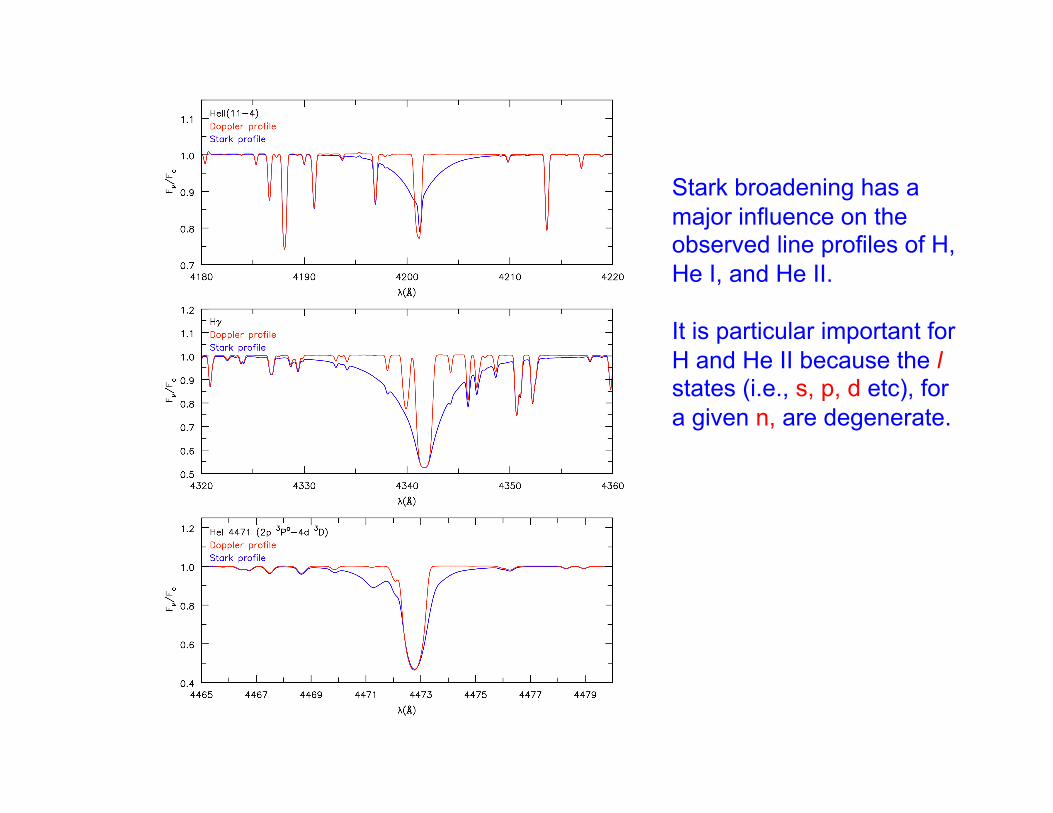
Stark broadening has a major influence on the observed line profiles of H, He I, and He II.

It is particular important for H and He II because the l states (i.e., s, p, d etc), for a given n, are degenerate.

ReasonsforPlaneParallelApproxima1on

Realstarsarespherical.However,wecanapproximatetheiratmospheresasplane‐parallelifthethicknessoftheatmosphereismuchlessthantheradiusofthestar.Todeterminetheatmospherethicknessweconsidertheforcesac1ngonasmallelementinsidethestar.

Thus

P(r+dr)

P(r)

Fg

dr dA The mass of the element of area dA is ρ.dA.dr where ρ is the density. The only forces acting on the element are gas pressure, and gravity. If the star is to be in equilibrium, these forces must be equal.

Define Mr as mass interior to radius r.

dm

Hence

ThisistheEQUATIONofHYDROSTATICEQUILIBIRUM.Itprovides(withotherequa1ons)ameansofdeterminingthestructureofthestar).

Weassumeonlygaspressurewasimportant.ThisistrueforstarsliketheSun,butforhot(orveryluminous)starsradia1onpressureMUSTbeincludedintheequa1onofhydrosta1cequilibrium.Inthepresentcontextweareinterestedonlyintheatmosphericlayers,andhenceMr=M*.Wewillalsoassumether=R*,thevalidityofwhichwillbechecked.Usingzasthedependentvariablewehave

whereisthestar’sSURFACEGRAVITY.Thepressureis

givenbytheidealgaslaw:

whereNpisthepar1cledensity,

kisBoltzmann’sconstant,and

Tisthegastemperature.

ThedensityisgivenbywhereweusemHtodenotetheatomicmassunit,andμpisthemeanpar1clemassinAMU(atomicamassunits).

Thus

Toes1matetheatmosphericscaleheightwewillassumetheatmosphereisisothermal(thedensitygenerallyvariesmuchmorethethetemperature).Thus

whichhassolu1on(byintegra1ngfromztoinfinty)

whereNoisthepar1cledensityatz=0,andhistheatmosphericscaleheight,andisgivenby

He II 4686

NV 4609

He II 4686

N III 4640

NIV 5058 He II (8-4) / Hβ

WN Stars He, N enriched / H, C, O deficient

CNO processed material at surface.

He II 1640Å

CIV 1548,1550Å

C III 1909Å

C III 6740Å C IV 5805Å C IV 4650Å

WC Stars He, C enriched / Zero H, N

He burning material at surface.

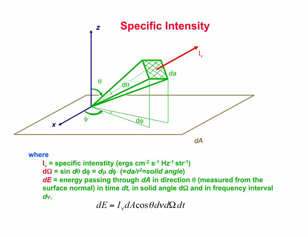
Specific Intensity

where Iν = specific intenstity (ergs cm-2 s-1 Hz-1 str-1) dΩ = sin dθ dφ = dµ dφ (=da/r2=solid angle) dE = energy passing through dA in direction θ (measured from the surface normal) in time dt, in solid angle dΩ and in frequency interval dν.

( θ

z

φ

dθ

Iν

x dφ

dA

da

Transfer Equation

Geometry-Free Transfer Equation

where Iν = specific intensity (ergs cm-2 s-1 Hz-1 sr-1) s = distance along path ην = emissivity (ergs cm-3 s-1 Hz-1 sr-1) χν = opacity (cm-1) Sν = source function (ergs cm-2 s-1 Hz-1 sr-1) τ = optical depth ( dτ = -χds)

ds

Iν(µ)

Plane-Parallel Transfer Equation

where z = spatial coordinate (directed outward, and normal to surface) µ = cos θ τ = optical depth ALONG z NB: dτ (ray) = -χ dz/µ

z

ds θ

Iν(µ)

z=constant

NB: Radiation field is assumed to be independent of azimuth (φ)

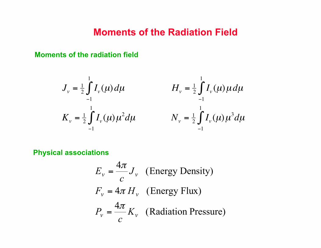
Moments of the Radiation Field

€

Jv = 12 Iv (µ)dµ−1

1

∫ Hv = 12 Iv (µ)µdµ−1

1

∫

Kv = 12 Iv (µ)µ

2dµ−1

1

∫ Nv = 12 Iv (µ)µ

3dµ−1

1

∫

Moments of the radiation field

Physical associations

Moment Transfer Equations

€

dHv

dz= χv (Sv − Jv )

€

dKv

dz= −χvHv

€

dHv

dτν= Jv − Sv

€

dKv

dτν= Hv

€

1r2dr2Hv

dz= χv (Sv − Jv )

€

1r2dr2Kv

dz+Kν − Jν

r= −χvHv€

dr2Hv

dτν= r2(Jv − Sv )

€

dr2Kv

dτν−r2(Kν − Jν )

χν r= r2Hv

Plane Parallel

Spherical

Formal Solution. Solve the transfer equation for I, with J and S known ---- FORMAL SOLUTION.

Timing per frequency: Plane parallel : ~ Nµ.ND

Spherical : ~ ND2 (as # of angle’s prop. to ND)

Use the formal solution to compute f (K/J), g (= N/H).

Moment Solution Solve for J (given thermal emission and opacity)

Timing per frequency: ~ ND

Linearized Moment Solution Solve for δJ Timing per frequency:

~ ND2 (other factors)

Notation

Choose grid (> 5 points per log τ). Define J, K on grid nodes [ i=1, outer boundary, i=ND inner boundary] Define H at mid points.

Thus

Solution of Moment Equations

where

Thus

where

(allows electron scattering to be taken into account)

These equations can be written in matrix form:

where T is a ND.ND tridiagonal matrix, and J and S are column vectors (length ND). Solved using Thomas Algorithm.

Boundary conditions: next slide

Linearization.

In matrix form

where F, G and R, are ND.ND matrices (not full), and dJ, dχ, dη, dθ are column vectors of length ND. This is easily solved for dJ (in terms of dχ, dη, dθ).

Accuracy Equations are second order accurate.

Inner boundary Use diffusion approximation.

Outer boundary. For plane-parallel, and spherical atmosphere can formulate a second order boundary condition for the Moment equations. For the CMF (comoving-frame) transfer equation not feasible. This can cause a loss of accuracy and instabilities. The later is removed by using a VERY SMALL step size at outer boundary. The instability is complicated and can cause J to blow up.

Choosing I(inward)=0 at outer boundary can cause problems as very difficult to extend atmosphere so that τ = 0 at all wavelengths. Can choose a very fine grid at outer boundary, but unphysical.

In CMGEN we extrapolate the opacities/emissivities at the outer boundary. This gives an I(inward) we can be used to define a b.c. for the outer boundary.

Notes

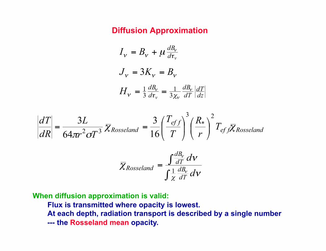
Diffusion Approximation

When diffusion approximation is valid: Flux is transmitted where opacity is lowest. At each depth, radiation transport is described by a single number --- the Rosseland mean opacity.

Saha- Boltzmann Equation (applies when Local Thermodynamic Equilibrium [LTE] is valid)

€

Nκ , j* = Ne

*Nκ +1,1* gκ , j

gκ +1,1

CI

T1.5exp(ψκ , j /kT)

Nl= population density (cm−3) of lower energy level, l

gl = degeneracy of statel = statistical weight hνlu= difference in energy ( * denotes LTE)

Relation between two level populations in the same ionization stage.

Relation between two populations in different (but consecutive) ionization stages.

Nκ,j = population of level j in ionization state κ Nκ+1,1 = population of level 1(g.s.) in ionization state κ+1 gκ,j = degeneracy of level j in ionization state κ gκ+1,j = degeneracy of g.s. in ionization state κ+1 ψκ ,j = ionization energy of state j

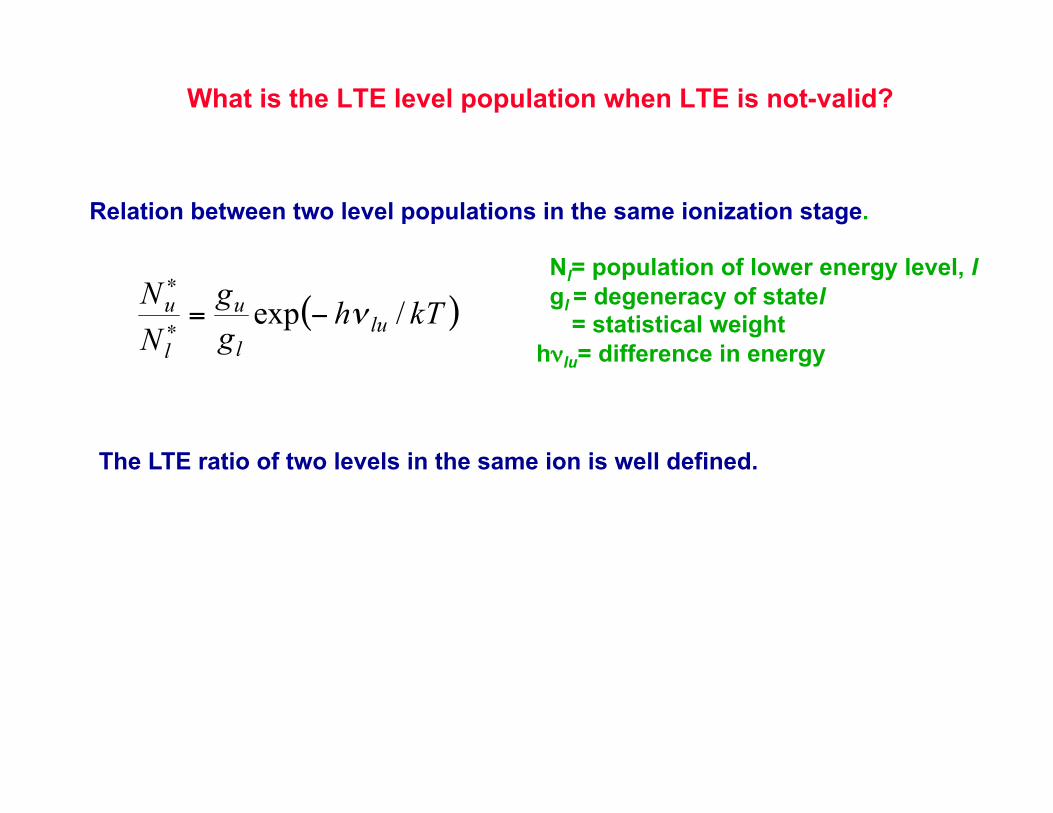
What is the LTE level population when LTE is not-valid?

Nl= population of lower energy level, l gl = degeneracy of statel = statistical weight hνlu= difference in energy

Relation between two level populations in the same ionization stage.

The LTE ratio of two levels in the same ion is well defined.

What is the LTE level population when LTE is not-valid?

€

Nκ , j* = NeNκ +1,1

gκ , jgκ +1,1

CI

T1.5exp(ψκ , j /kT)

Define the LTE population by the Saha equation using the actual ion density and the actual electron density.

€

Nκ , j*

= NeNκ +1,u

gκ , jgκ +1,u

CI

T1.5exp([ψκ , j + hνκ +1,1u]/kT)

However, there is no longer a unique LTE definition. Can define LTE, for example, with respect to another level in the next ionization stage.

If we define

then

€

N κ , j* =

bκ +1,u

bκ +1,1

Nκ , j*

€

bκ +1,u = Nκ +1,u /Nκ +1, j*

2p

1s

3s

2s

3d

Continuum

Energy

hν

h(ν -ν3d)

Sources of Opacity

Bound-free

€

χ j (v) =α(ν ) j N j − N j* exp(−hν /kT)( )

( α = photoionization cross-section)

Population of level j

LTE population of level j Cross-section (cm2) – set by atomic physics.

Ionizations to excited states

Consider C III (i.e., C2+). Then

C III 2s nl + hν <−−> C IV 2s + e−

but we also can have

C III 2p nl + hν <−−> C IV 2p + e−

The expression

€

χ j (v) = αv N j − N j* exp(−hν /kT)( )

is valid for both processes, provided we use the the correct LTE population --- the LTE that is defined with respect to the actual ion involved ( i.e, C IV 2s of C IV 2p).

Multi-electron systems can have states that lie above the ionization limit. If the state satisfies certain selection rules (e.g., parity) this state can autoionize to the ion and a free electron. The autoionization rates can be large (1014) and thus the doubly exited state is in LTE with respect to the ion. Instead of autoionizing, the state can undergo a bound-bound decay which moves it below the ionization limit, and hence cause a ``recombination’’. The reverse process can also occur, and appear as resonances in the photoionization cross-section.

e.g. CIII 2p nl : For high b, 2p electron decays. For these states to be populated, T large (although not very large for CIII) and the process is referred to as HTDR (high temperature dielectronic recombination).

When the 2p nl state is very close to the ionization limit (which occurs for low n e.g., 4) the state can provide an effective recombination rate at low temperatures. Rates are sensitive to the precise location of the atomic energy levels, and hence atomic physics. For many of the levels, the decay of the nl state may provide the dominate recombination route (Low TDR)

Resonance in Photoionization Cross-sections

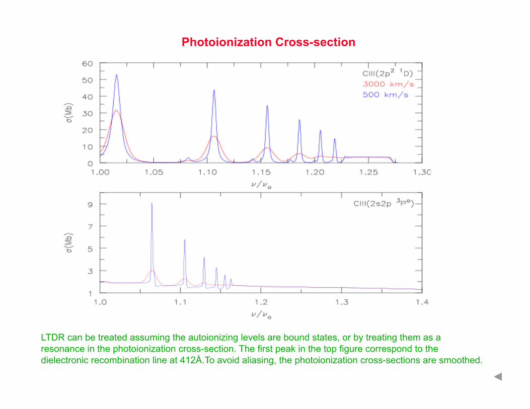
Photoionization Cross-section

LTDR can be treated assuming the autoionizing levels are bound states, or by treating them as a resonance in the photoionization cross-section. The first peak in the top figure correspond to the dielectronic recombination line at 412Å.To avoid aliasing, the photoionization cross-sections are smoothed.