basics of linux, gnuplot, c visualization of numerical data roots
TRANSCRIPT
1Physics 3340 - Fall 2016
Class Progress
Basics of Linux, gnuplot, CVisualization of numerical dataRoots of nonlinear equations (Midterm 1)Solutions of systems of linear equationsSolutions of systems of nonlinear equationsMonte Carlo simulationInterpolation of sparse data pointsNumerical integration (Midterm 2)Solutions of ordinary differential equations
2Physics 3340 - Fall 2016
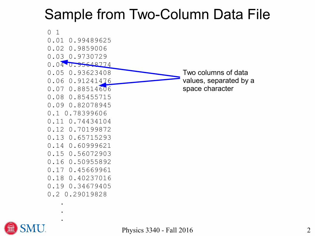
Sample from Two-Column Data File0 10.01 0.994896250.02 0.98590060.03 0.97307290.04 0.956487740.05 0.936234080.06 0.912414760.07 0.885146060.08 0.854557150.09 0.820789450.1 0.783996060.11 0.744341040.12 0.701998720.13 0.657152930.14 0.609996210.15 0.560729030.16 0.509558920.17 0.456699610.18 0.402370160.19 0.346794050.2 0.29019828 . . .
Two columns of data values, separated by a space character
3Physics 3340 - Fall 2016
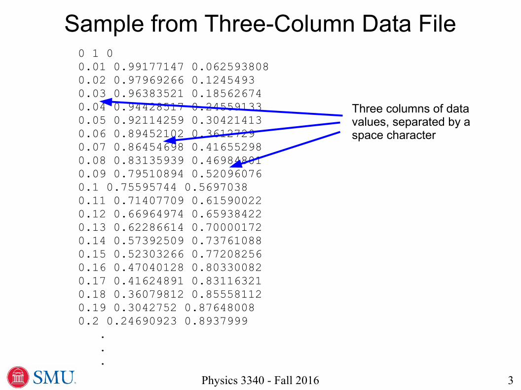
Sample from Three-Column Data File0 1 0 0.01 0.99177147 0.062593808 0.02 0.97969266 0.1245493 0.03 0.96383521 0.18562674 0.04 0.94428517 0.24559133 0.05 0.92114259 0.30421413 0.06 0.89452102 0.3612729 0.07 0.86454698 0.41655298 0.08 0.83135939 0.46984801 0.09 0.79510894 0.52096076 0.1 0.75595744 0.5697038 0.11 0.71407709 0.61590022 0.12 0.66964974 0.65938422 0.13 0.62286614 0.70000172 0.14 0.57392509 0.73761088 0.15 0.52303266 0.77208256 0.16 0.47040128 0.80330082 0.17 0.41624891 0.83116321 0.18 0.36079812 0.85558112 0.19 0.3042752 0.87648008 0.2 0.24690923 0.8937999 . . .
Three columns of data values, separated by a space character
4Physics 3340 - Fall 2016
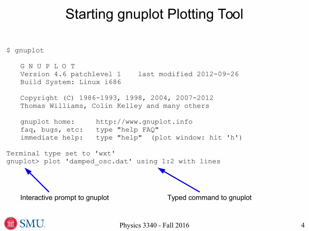
$ gnuplot
G N U P L O TVersion 4.6 patchlevel 1 last modified 2012-09-26 Build System: Linux i686
Copyright (C) 1986-1993, 1998, 2004, 2007-2012Thomas Williams, Colin Kelley and many others
gnuplot home: http://www.gnuplot.infofaq, bugs, etc: type "help FAQ"immediate help: type "help" (plot window: hit 'h')
Terminal type set to 'wxt'gnuplot> plot 'damped_osc.dat' using 1:2 with lines
Starting gnuplot Plotting Tool
Typed command to gnuplotInteractive prompt to gnuplot
5Physics 3340 - Fall 2016
gnuplot Command Language Example
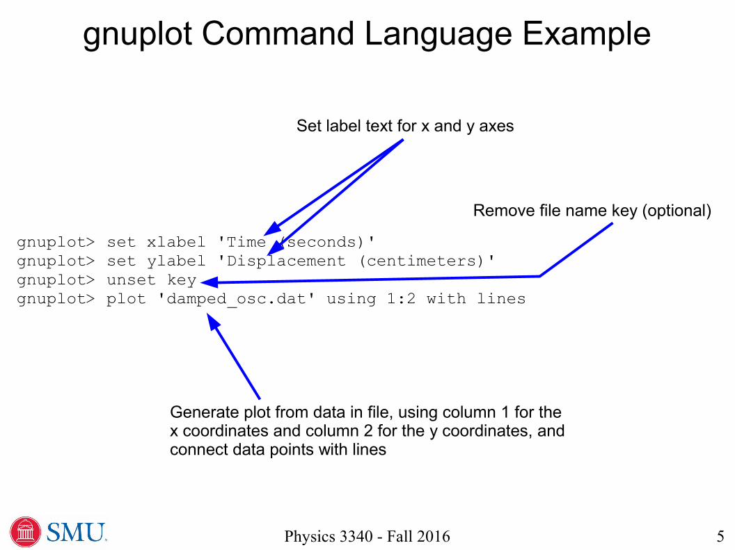
gnuplot> set xlabel 'Time (seconds)'gnuplot> set ylabel 'Displacement (centimeters)'gnuplot> unset keygnuplot> plot 'damped_osc.dat' using 1:2 with lines
Set label text for x and y axes
Remove file name key (optional)
Generate plot from data in file, using column 1 for the x coordinates and column 2 for the y coordinates, and connect data points with lines
6Physics 3340 - Fall 2016
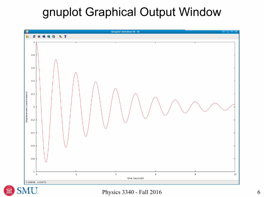
gnuplot Graphical Output Window
7Physics 3340 - Fall 2016
gnuplot Command Language Example
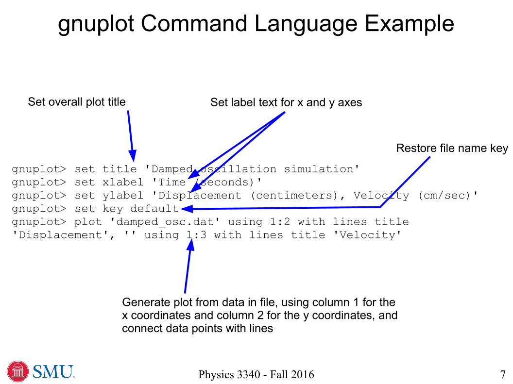
gnuplot> set title 'Damped oscillation simulation'gnuplot> set xlabel 'Time (seconds)'gnuplot> set ylabel 'Displacement (centimeters), Velocity (cm/sec)'gnuplot> set key defaultgnuplot> plot 'damped_osc.dat' using 1:2 with lines title 'Displacement', '' using 1:3 with lines title 'Velocity'
Set overall plot title
Restore file name key
Generate plot from data in file, using column 1 for the x coordinates and column 2 for the y coordinates, and connect data points with lines
Set label text for x and y axes
8Physics 3340 - Fall 2016
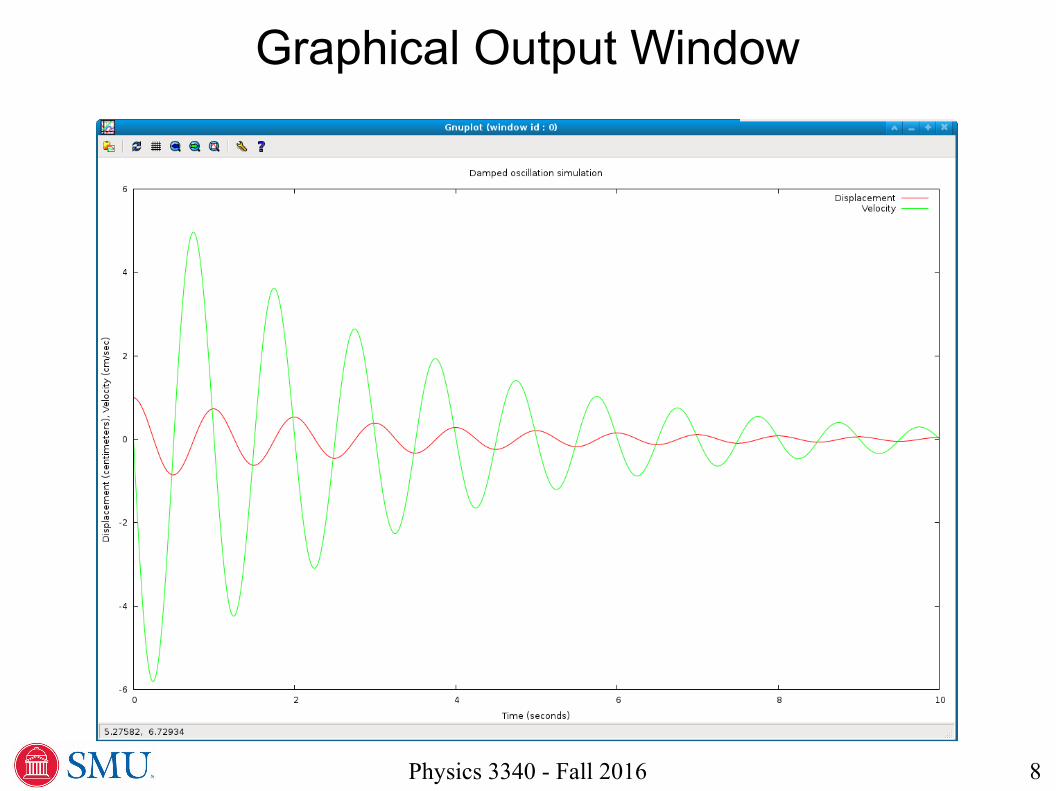
Graphical Output Window
9Physics 3340 - Fall 2016
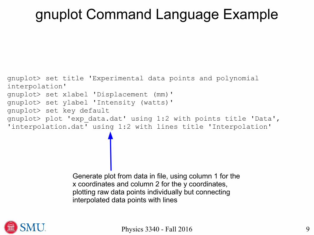
gnuplot Command Language Example
gnuplot> set title 'Experimental data points and polynomial interpolation'gnuplot> set xlabel 'Displacement (mm)'gnuplot> set ylabel 'Intensity (watts)'gnuplot> set key defaultgnuplot> plot 'exp_data.dat' using 1:2 with points title 'Data', 'interpolation.dat' using 1:2 with lines title 'Interpolation'
Generate plot from data in file, using column 1 for the x coordinates and column 2 for the y coordinates, plotting raw data points individually but connecting interpolated data points with lines
10Physics 3340 - Fall 2016
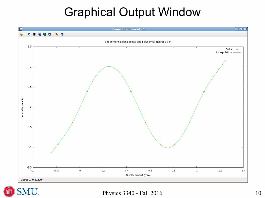
Graphical Output Window
11Physics 3340 - Fall 2016
Generating Graphics for Documents
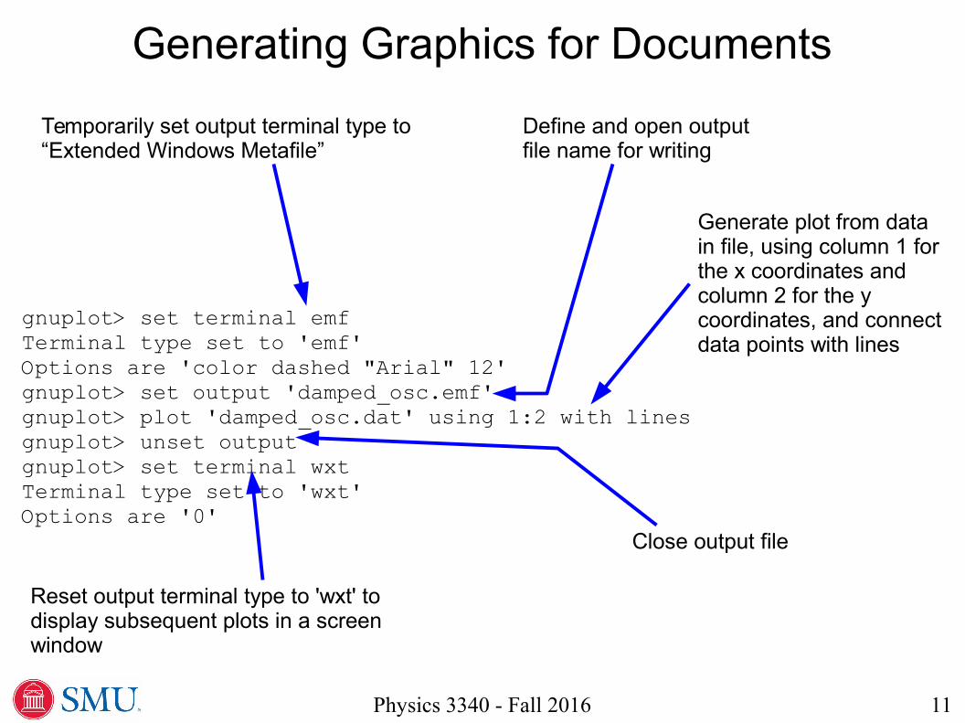
gnuplot> set terminal emfTerminal type set to 'emf'Options are 'color dashed "Arial" 12'gnuplot> set output 'damped_osc.emf'gnuplot> plot 'damped_osc.dat' using 1:2 with linesgnuplot> unset outputgnuplot> set terminal wxtTerminal type set to 'wxt'Options are '0'
Generate plot from data in file, using column 1 for the x coordinates and column 2 for the y coordinates, and connect data points with lines
Reset output terminal type to 'wxt' to display subsequent plots in a screen window
Close output file
Temporarily set output terminal type to “Extended Windows Metafile”
Define and open output file name for writing
12Physics 3340 - Fall 2016
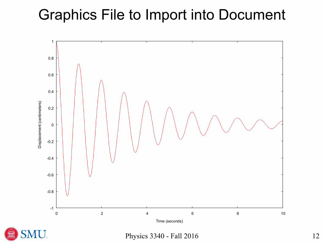
Graphics File to Import into Document
-1
-0.8
-0.6
-0.4
-0.2
0
0.2
0.4
0.6
0.8
1
0 2 4 6 8 10
Dis
pla
cem
ent
(ce
ntim
ete
rs)
Time (seconds)
13Physics 3340 - Fall 2016
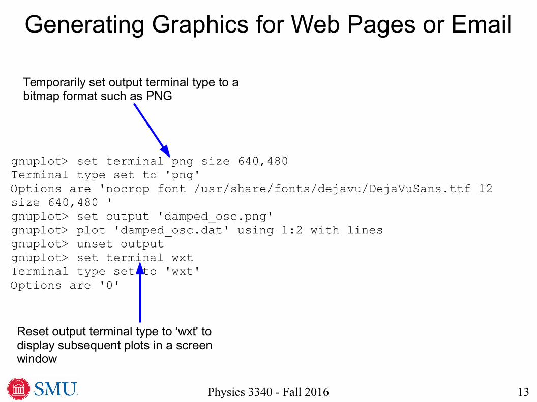
Generating Graphics for Web Pages or Email
gnuplot> set terminal png size 640,480Terminal type set to 'png'Options are 'nocrop font /usr/share/fonts/dejavu/DejaVuSans.ttf 12 size 640,480 'gnuplot> set output 'damped_osc.png'gnuplot> plot 'damped_osc.dat' using 1:2 with linesgnuplot> unset outputgnuplot> set terminal wxtTerminal type set to 'wxt'Options are '0'
Reset output terminal type to 'wxt' to display subsequent plots in a screen window
Temporarily set output terminal type to a bitmap format such as PNG
14Physics 3340 - Fall 2016
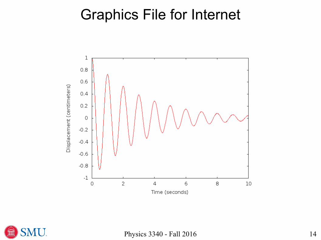
Graphics File for Internet
15Physics 3340 - Fall 2016
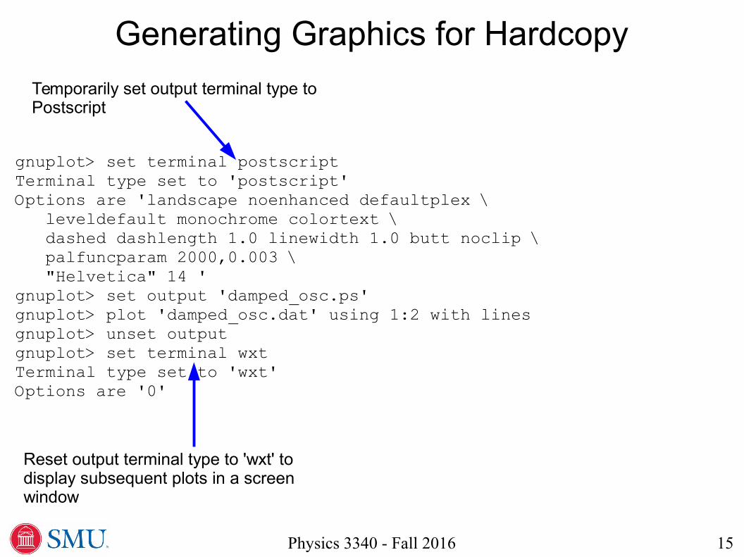
Generating Graphics for Hardcopy
gnuplot> set terminal postscriptTerminal type set to 'postscript'Options are 'landscape noenhanced defaultplex \ leveldefault monochrome colortext \ dashed dashlength 1.0 linewidth 1.0 butt noclip \ palfuncparam 2000,0.003 \ "Helvetica" 14 'gnuplot> set output 'damped_osc.ps'gnuplot> plot 'damped_osc.dat' using 1:2 with linesgnuplot> unset outputgnuplot> set terminal wxtTerminal type set to 'wxt'Options are '0'
Reset output terminal type to 'wxt' to display subsequent plots in a screen window
Temporarily set output terminal type to Postscript
16Physics 3340 - Fall 2016
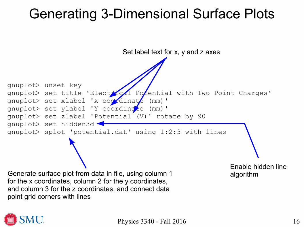
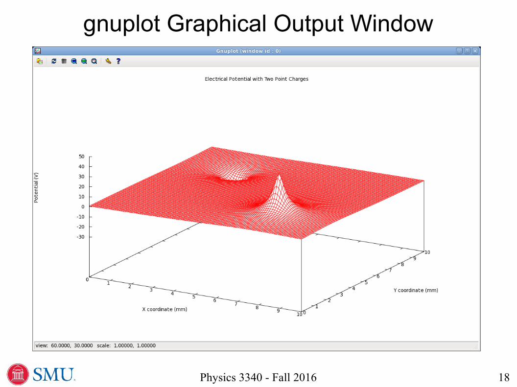
Generating 3-Dimensional Surface Plots
gnuplot> unset keygnuplot> set title 'Electrical Potential with Two Point Charges'gnuplot> set xlabel 'X coordinate (mm)'gnuplot> set ylabel 'Y coordinate (mm)'gnuplot> set zlabel 'Potential (V)' rotate by 90gnuplot> set hidden3dgnuplot> splot 'potential.dat' using 1:2:3 with lines
Set label text for x, y and z axes
Generate surface plot from data in file, using column 1 for the x coordinates, column 2 for the y coordinates, and column 3 for the z coordinates, and connect data point grid corners with lines
Enable hidden line algorithm
17Physics 3340 - Fall 2016
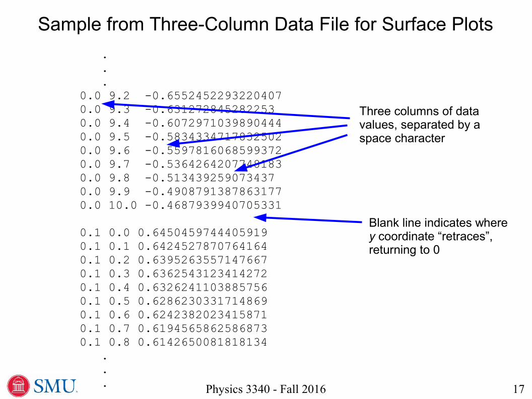
Sample from Three-Column Data File for Surface Plots
. . .0.0 9.2 -0.65524522932204070.0 9.3 -0.6312728452822530.0 9.4 -0.60729710398904440.0 9.5 -0.58343347178325020.0 9.6 -0.55978160685993720.0 9.7 -0.53642642077481830.0 9.8 -0.5134392590734370.0 9.9 -0.49087913878631770.0 10.0 -0.4687939940705331
0.1 0.0 0.64504597444059190.1 0.1 0.64245278707641640.1 0.2 0.63952635571476670.1 0.3 0.63625431234142720.1 0.4 0.63262411038857560.1 0.5 0.62862303317148690.1 0.6 0.62423820234158710.1 0.7 0.61945658625868730.1 0.8 0.6142650081818134 . . .
Three columns of data values, separated by a space character
Blank line indicates where y coordinate “retraces”, returning to 0
18Physics 3340 - Fall 2016
gnuplot Graphical Output Window
19Physics 3340 - Fall 2016
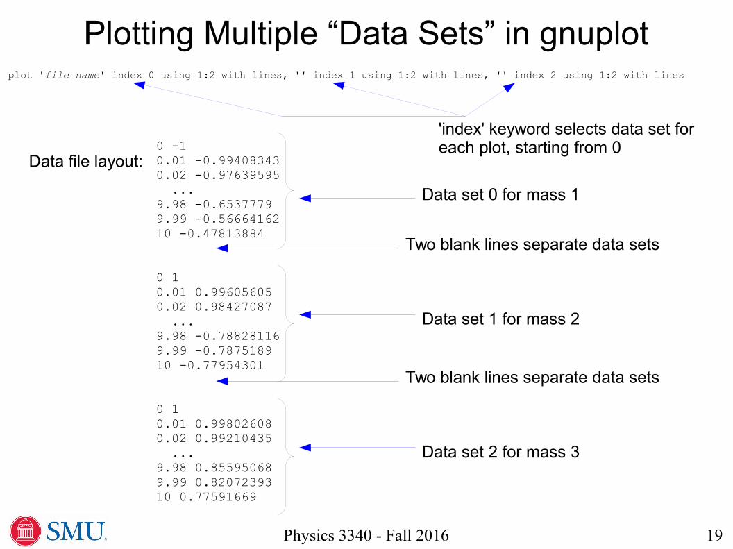
Plotting Multiple “Data Sets” in gnuplotplot 'file name' index 0 using 1:2 with lines, '' index 1 using 1:2 with lines, '' index 2 using 1:2 with lines
0 -10.01 -0.994083430.02 -0.97639595 ...9.98 -0.65377799.99 -0.5666416210 -0.47813884
0 10.01 0.996056050.02 0.98427087 ...9.98 -0.788281169.99 -0.787518910 -0.77954301
0 10.01 0.998026080.02 0.99210435 ...9.98 0.855950689.99 0.8207239310 0.77591669
Data file layout:
Data set 1 for mass 2
Data set 2 for mass 3
Data set 0 for mass 1
Two blank lines separate data sets
Two blank lines separate data sets
'index' keyword selects data set for each plot, starting from 0
20Physics 3340 - Fall 2016
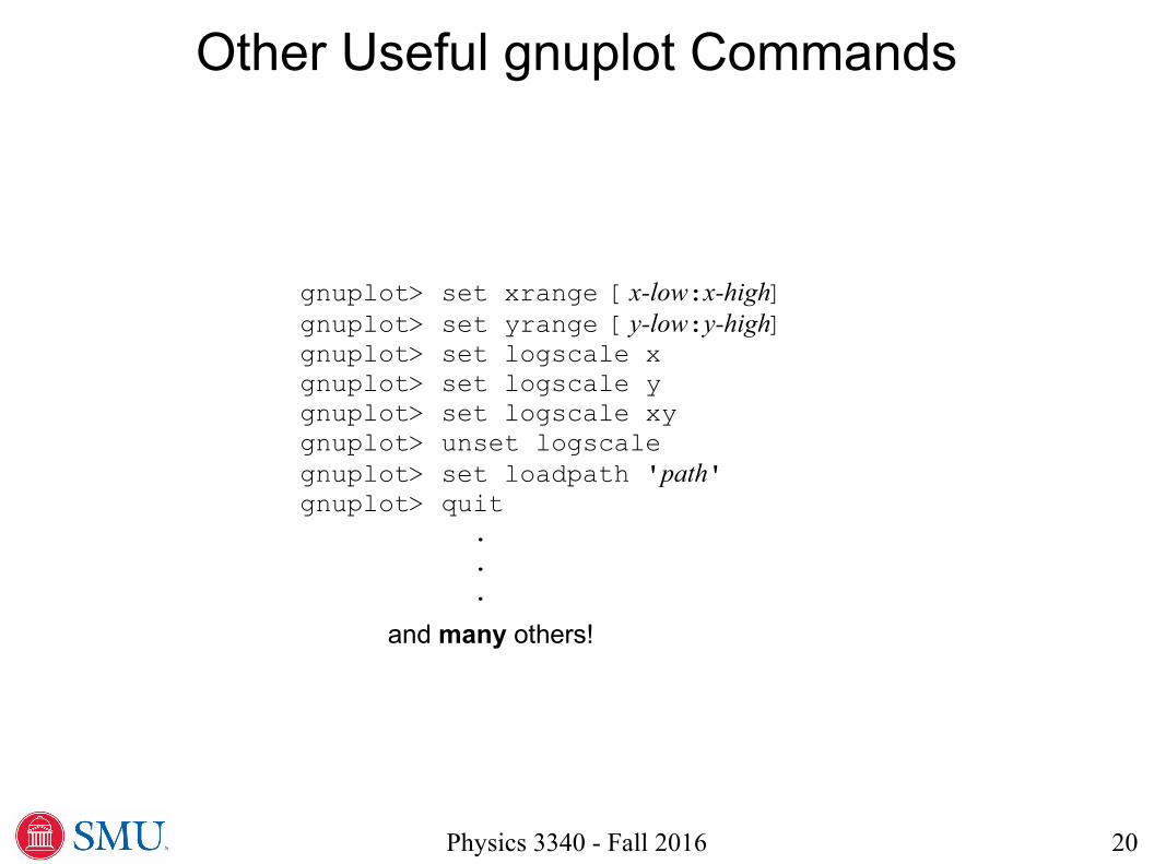
Other Useful gnuplot Commands
gnuplot> set xrange [x-low:x-high]gnuplot> set yrange [y-low:y-high]gnuplot> set logscale xgnuplot> set logscale ygnuplot> set logscale xygnuplot> unset logscalegnuplot> set loadpath 'path'gnuplot> quit . . .
and many others!