basic statistical tools - unesp · structural health monitoring using statistical pattern...
TRANSCRIPT

Structural Health Monitoring UsingStatistical Pattern Recognition
Basic Statistical Tools
Los Alamos Dynamics Structural Dynamics and Mechanical Vibration Consultants
Presented by
Charles R. Farrar, Ph.D., P.E.
Los Alamos Dynamics Structural Dynamics and Mechanical Vibration Consultants 2
Overview
• Provide a brief statistics background to help with further discussions of statistical pattern recognition applied to Structural Health Monitoring.– Probability Density Function
– Cumulative Distribution Function
– Statistical Moments
– Density Estimation
– Confidence Limits
– Central Limit Theorem
– Multivariate statistics
– Multivariate Analysis
– Curse of Dimensionality
– Assessment of normality
– Data Reduction/Compression

Los Alamos Dynamics Structural Dynamics and Mechanical Vibration Consultants 3
• First, we need to define the Probability Density Function, fx(x), which is used to quantify the Probability Distribution.
• A Probability Density Function describes the probability density over the sample space of a continuous random variable, X.
• The probability that X lies between a and b is given by:
• Some properties:
Probability Density Functions
b
ax dx)x(f)bXa(P
1dx)x(f,0)x(f xx
b a
fx(X)
X
Probability Density Function
Los Alamos Dynamics Structural Dynamics and Mechanical Vibration Consultants 4
Probability Density Functions
• Some common probability density functions:– Gaussian or Normal Distribution
• Standard normal distribution: x=0, 2=1
– Rayleigh Distribution
• Describes the distance a particle travels per unit time when subjected to velocity components described by normal distributions
2
x
xx21
xx e
21
)x(f
0x,eb
x)x(f
2
bx
21
2x
-4 -2 0 2 40
0.1
0.2
0.3
0.4
0 0.5 1 1.5 20
0.5
1
1.5
ResizeLegendb = 0.5

Los Alamos Dynamics Structural Dynamics and Mechanical Vibration Consultants 5
Probability Density Functions
• Log-Normal Distribution
– Used when values of random variable are know to be positive, e.g. fatigue life.
• Weibull Distribution
– Models failure of materials
)x(ln),x(lnEwhere
x0,ex2
1)x(f
2
xln21
x
2
,ex
)x(fx1
x
0 1 2 30
0.5
1
1.5
ResizeLegend
0 2 4 6 8 100
0.5
1
1.5
Median = 1.0
=10 =5.0
=0.1
=0.3
=0.5
Los Alamos Dynamics Structural Dynamics and Mechanical Vibration Consultants 6
Cumulative Distribution Function
• The Cumulative Distribution Function, F(x), defines the probability that a random variable X is less than or equal to some value x.
• If Fx(x) has a first derivative, the following relationship between the cumulative distribution function and the probability density function holds:
x
xx d)(f)xX(P)x(F
dx)x(dF
)x(f xx

Los Alamos Dynamics Structural Dynamics and Mechanical Vibration Consultants 7
Cumulative Distribution Function
• Some properties of Fx(x): 0)x(F1)(F,0)(F xxx
-0.5 0 0.5 10
0.5
1
1.5
2
2.5
Bimodal PDF
Bimodal CDF
Los Alamos Dynamics Structural Dynamics and Mechanical Vibration Consultants 8
Statistical Moments
• We will be interested in calculating the average behavior of a random variable (in our case some damage sensitive feature) and estimating how frequently significant deviations from the average occur.
• The mean value, x, (a.k.a. expected value, E(x)) provides a measure of the this average behavior.
• The mean value is defined by the following formula for a continuous random variable:
dx)x(fx)x(E xx n
xˆxE
n
1ii
x
x is a parameter in a model x is estimated from discrete data

Los Alamos Dynamics Structural Dynamics and Mechanical Vibration Consultants 9
Statistical Moments
• The mean value can be thought of in terms of a mechanics analogy as the first moment of the density function (for such calculations one typically divides by total area, but for PDF’s that area is one)
x
dx
fx(x) dx
fx(X)
X
Probability Density Function
dx)x(fx xx
Los Alamos Dynamics Structural Dynamics and Mechanical Vibration Consultants 10
Statistical Moments
• The mean value provide a measure of the random variable’s central tendency.
• There are other measures of a random variable’s central tendency:– Mode (or modal value) is the most probable value of a
random variable (corresponds to the highest point in the probability density function).
– Median is the value of a random variable where values above and below this one are equally probable.
• For a uni-modal, symmetric probability density function (e.g. Guassian or normal density function), the mean, the mode and the median are identical.

Los Alamos Dynamics Structural Dynamics and Mechanical Vibration Consultants 11
Statistical Moments
• Variance, , provides a first order measure of the dispersion of the random variables from the mean.
• The Variance is defined as:
• The Standard Deviation, x , and Coefficient of Variation, Cx , also provide a measure of the dispersion from the mean.
n
xn
i
2xi
2x
2x
dx)x(fx x2
x2x
x
xx
2xx C,
is a parameter in a model2x is estimated from discrete data
2x
Los Alamos Dynamics Structural Dynamics and Mechanical Vibration Consultants 12
Statistical Moments
• Variance can be thought of as the second moment of the probability density function about the mean.
x
x-x
dx
fx(x) dx
fx(X)
X
Probability Density Function
dx)x(fx x2
x2x

Los Alamos Dynamics Structural Dynamics and Mechanical Vibration Consultants 13
Statistical Moments
• The mean and standard deviation are used for standard data normalization:
• This normalized random variable Z will have zero mean and a variance of 1
x
xXZ
• Need to consider the difference between the variance of the sample and the variance of the population.
• When estimating the variance of the population from a sample, divide previous equation for discrete data by (N-1) instead of N (for large samples this is not an issue).
Los Alamos Dynamics Structural Dynamics and Mechanical Vibration Consultants 14
Biased vs Unbiased Estimators
• An estimate of a statistic is said to be unbiased if the mean of the statistics obtained from individual samples is equal to the statistic for the entire population.

Los Alamos Dynamics Structural Dynamics and Mechanical Vibration Consultants 15
Biased vs Unbiased Estimates
• Biased estimate of Variance
• Unbiased estimate of variance
N
XN
1i
2xi
2x
1N
XN
1i
2xi
2x
Los Alamos Dynamics Structural Dynamics and Mechanical Vibration Consultants 16
Biased vs Unbiased Estimates• Biased vs Unbaised Estimators• % An estimate of a statistic is said to be unbiased if the mean of the• % statistics obtained from individual samples is equal to the statistic for• % the entire population.• %• % Lets begin by looking at a 10000 pt uniformly distributed random signal• x=rand(1,10000);• plot (x)• % Now calculate the variance of the entire population noting that by default Matlab• % calculates an unbiased estimate of the variance (the arguement 1 in the• % var command provides a biased variance estimate where the variance is normalized by
the number of• % samples, n)• vpop=var(x,1)• %Next, break the signal into 1000 intervals and calculate the variance for each• %of these samples using biased variance estimate (arguement 1 specified, i.e. normalize by
n).• for i=1:1000• j=i-1;• vint(1,i)=var(x(1,((j*10)+1):(10*i)),1);• end• %Calculate the mean of the sample variances• mvsample=mean(vint)• %Because the mean of the sample variances is not equal to the variance of the entire• %population, the variance estimatenormalized by n is said to be a baised estimate of the
population variance.• %• %Now calculate the unbiased estimate of the sample variance (normalize by n-1, • %where n is sample size, this is Matlab default)and show that• %the mean of these variance estimates equals the variance of the• %population.• for i=1:1000• j=i-1;• vbar(i)=var(x(1,((j*10)+1):(10*(i))));• end• mvbar=mean(vbar)• %• %Finally, note that the difference between the biased estimate and• %the unbiased estimate becomes small a
Variance of 10000 pt population of uniformly distributed random variable between 0 and 1
pop=0.0835
Mean of biased Variances from 1000 10-pt samples of same random variableMean2
sample=0.0751
Mean of unbiased estimates of Variances from 1000 10-pt samples of same random variableMean2
sample=0.0834
Los Alamos Dynamics Structural Dynamics and Mechanical Vibration Consultants 17
fx(X)
X
Positive SkewnessNegative Skewness
Statistical Moments
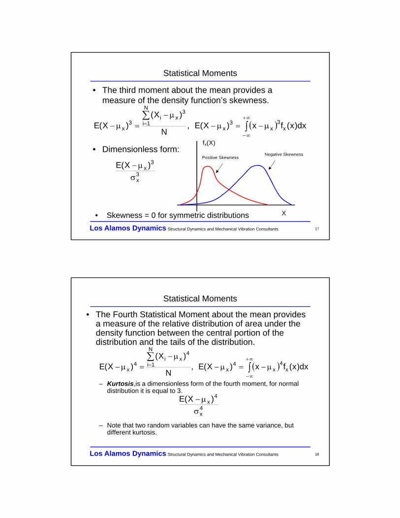
• The third moment about the mean provides a measure of the density function’s skewness.
• Dimensionless form:
dx)x(fx)X(E,N
)X()X(E x
3x
3x
N
1i
3xi
3x
3x
3x )X(E
• Skewness = 0 for symmetric distributions
Los Alamos Dynamics Structural Dynamics and Mechanical Vibration Consultants 18
• The Fourth Statistical Moment about the mean provides a measure of the relative distribution of area under the density function between the central portion of the distribution and the tails of the distribution.
– Kurtosis,is a dimensionless form of the fourth moment, for normal distribution it is equal to 3.
– Note that two random variables can have the same variance, but different kurtosis.
Statistical Moments
dx)x(fx)X(E,N
)X()X(E x
4x
4x
N
1i
4xi
4x
4x
4x )X(E

Los Alamos Dynamics Structural Dynamics and Mechanical Vibration Consultants 19
Statistical Moments
x
fx(X)
• Two normal distributions with the same mean- Fourth moments about the mean are different- Non-dimensional fourth moment, or kurtosis, will be the
same for each distribution and equal to 3
Los Alamos Dynamics Structural Dynamics and Mechanical Vibration Consultants 20
Density Estimation
• Density estimation is the process of estimating an unknown probability density function based on data sampled from the corresponding random process.
• There are two general approaches to density estimation:– Parametric density estimation where we assume the form
of the density function (e.g. normal distribution) a priori.
– Non-parametric density estimation where we let the data define the density function
• Origins in 1950s
• A method to free discriminant analysis from rigid distribution assumptions
Los Alamos Dynamics Structural Dynamics and Mechanical Vibration Consultants 21
Parametric Density Estimation
• Person doing the data interrogation chooses a density form a priori.
• Probability density function will depend on unknown parameters.
• For the case where fx(x) is assumed to be a normal distribution, parametric density estimation reduces to finding the mean, x, and standard deviation, x.
• Estimate x and x from the observed data.
• This density estimation procedure is powerful if the assumed form of the density is correct.
Los Alamos Dynamics Structural Dynamics and Mechanical Vibration Consultants 22
Nonparametric Density Estimation
• Allows the observed data to “choose” the form of the density.– Histogram density estimator.
– Naive density estimator.
– Kernel density estimator.
• All these methods have “fit” parameters that must be specified and these parameters influence the shape and smoothness of the estimated density function.
• No unique solution.

Los Alamos Dynamics Structural Dynamics and Mechanical Vibration Consultants 23
• Oldest and most widely used form of density estimate.
• Choose origin, x0, and bin width, h• Bins are defined as [x0+mh, x0+(m+1)h) for positive and negative
m values.• Can use variable bin widths.• Choice of bin width controls the amount of smoothing in the
estimate.• For given bin width, choice of the origin can have a significant
effect on appearance of the density estimate.
Histogram Estimator
)x as bin same in )i(x of(# nh1
)x(f̂x
Los Alamos Dynamics Structural Dynamics and Mechanical Vibration Consultants 24
Histogram Estimator
-5 0 5 10 150
50
100
150
200
ResizeLegend
-5 0 5 10 150
100
200
300
400
500
600
ResizeLegend
10 bins 30 bins

Los Alamos Dynamics Structural Dynamics and Mechanical Vibration Consultants 25
Naive Estimator
• Now construct a histogram where each point is the center of a sampling interval by placing a box of width 2h and height (2nh)-1 on each observation and sum the results.
otherwise0,1x,2/1)x(w
,h
Xxw
h1
n1
)X(f in
1ix
Los Alamos Dynamics Structural Dynamics and Mechanical Vibration Consultants 26
Naive Estimator
fx(X)
XXX X X X X
(2nh)-1
2h
Place box shown at right on each observation and sum boxes to obtain density estimate
Los Alamos Dynamics Structural Dynamics and Mechanical Vibration Consultants 27
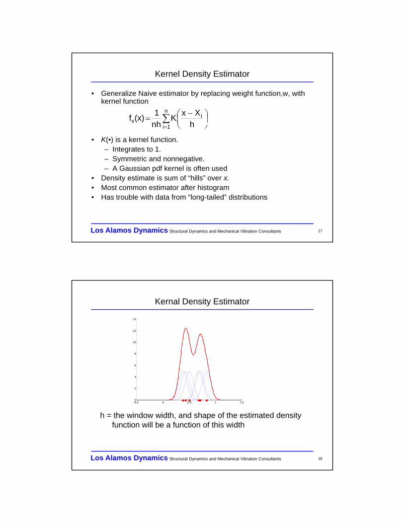
• Generalize Naive estimator by replacing weight function,w, with kernel function
• K(•) is a kernel function.– Integrates to 1.– Symmetric and nonnegative.– A Gaussian pdf kernel is often used
• Density estimate is sum of “hills” over x.• Most common estimator after histogram• Has trouble with data from “long-tailed” distributions
Kernel Density Estimator
n
1i
ix h
XxK
nh1
(x)f
Los Alamos Dynamics Structural Dynamics and Mechanical Vibration Consultants 28
Kernal Density Estimator
h = the window width, and shape of the estimated density function will be a function of this width
-0.5 0 0.5 1 1.50
2
4
6
8
10
12
14

Los Alamos Dynamics Structural Dynamics and Mechanical Vibration Consultants 29
3-Story Test Structure
Los Alamos Dynamics Structural Dynamics and Mechanical Vibration Consultants 30
Kernel Density Estimator Applied to 4 DOF Structure
Impact Nonlinearity, Amplitude 2.0 v rmsSkewness =
Linear System, Amplitude 2.0 v rmsSkewness
Impact Nonlinearity, Amplitude 0.5 v RMSSkewnes
Linear System, Amplitude 0.5 v RMSSkewness

Los Alamos Dynamics Structural Dynamics and Mechanical Vibration Consultants 31
Central Limit Theorem
• The Central Limit Theorem states that the distribution of a sum of random variables tends to the normal distribution as the number of random variables increases, regardless of these random variables’ individual distributions.
• Example: 1000 realizations of sum of n random variables drawn from a binomial distribution.
-1.5 -1 -0.5 0 0.5 1 1.50
100
200
300
400
500
600
-3 -2 -1 0 1 2 30
50
100
150
200
250
-4 -3 -2 -1 0 1 2 3 40
10
20
30
40
50
60
70
80
90
N=2 N=10 N=100
Los Alamos Dynamics Structural Dynamics and Mechanical Vibration Consultants 32
Confidence Intervals
• For a random variable, X, whose probability distribution is defined by some probability density function fx(X), the confidence intervals define a range of values that there is high probability (not certainty) will contain a realization of X.
• Notation: is the confidence level (e.g. 95%, 99%)
• For normal distribution some confidence levels can be related to the mean, x, and standard deviation, x.
21 XXXCONF
xxxx
xxxx
xxxx
3X3%73.99
and,2X2%45.95
,X%27.68
Los Alamos Dynamics Structural Dynamics and Mechanical Vibration Consultants 33
Confidence Intervals
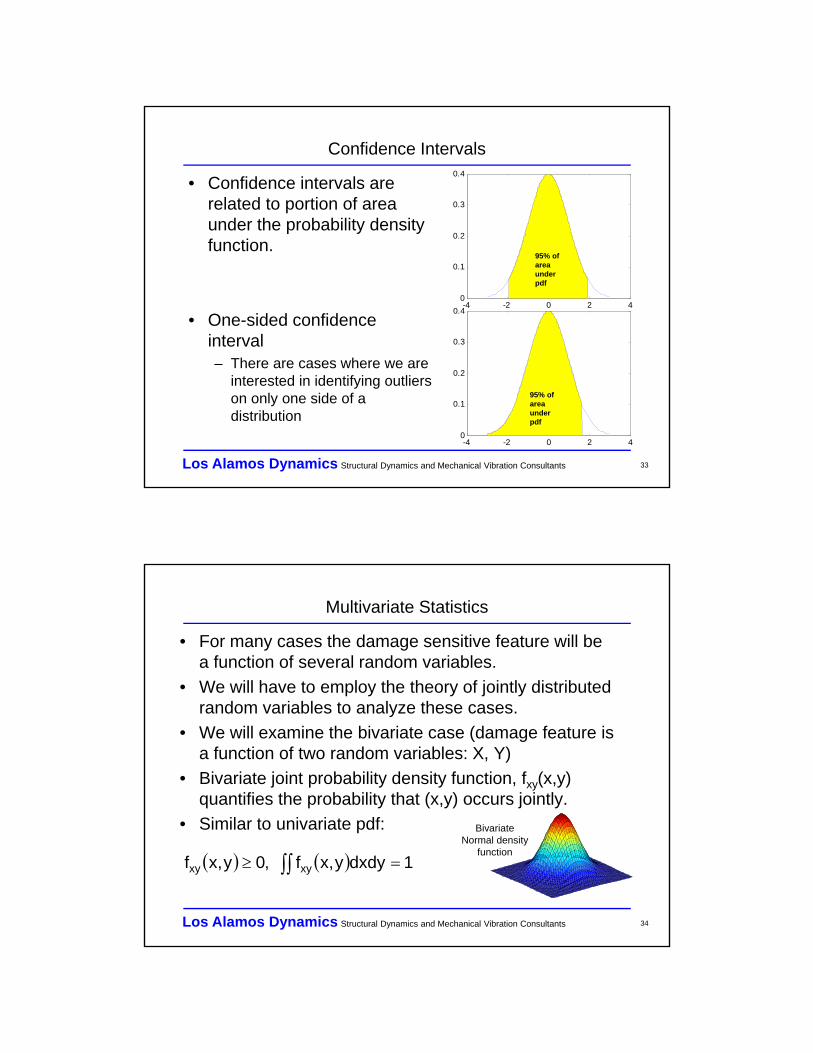
• Confidence intervals are related to portion of area under the probability density function.
• One-sided confidence interval– There are cases where we are
interested in identifying outliers on only one side of a distribution
-4 -2 0 2 40
0.1
0.2
0.3
0.4
-4 -2 0 2 40
0.1
0.2
0.3
0.4
95% of area under pdf
95% of area under pdf
Los Alamos Dynamics Structural Dynamics and Mechanical Vibration Consultants 34
Multivariate Statistics
• For many cases the damage sensitive feature will be a function of several random variables.
• We will have to employ the theory of jointly distributed random variables to analyze these cases.
• We will examine the bivariate case (damage feature is a function of two random variables: X, Y)
• Bivariate joint probability density function, fxy(x,y) quantifies the probability that (x,y) occurs jointly.
• Similar to univariate pdf:
1dxdyy,xf,0y,xf xyxy
BivariateNormal density
function

Los Alamos Dynamics Structural Dynamics and Mechanical Vibration Consultants 35
Multivariate Statistics
• Bivariate Cumulative Density Function:
• Marginal Density Functions
)y,x(Fyx
y,xf
)yYxX(Pdudvv,uf)y,x(F
Y,X
2
Y,X
xxy
yY,X
dx)y,x(f)x(f
dy)y,x(f)x(f
XYY
XYX
X
Y
x
y
X
fX(x)fX(x)dx
Los Alamos Dynamics Structural Dynamics and Mechanical Vibration Consultants 36
Multivariate Statistics
• Moments of jointly distributed random variables:– E[XnYm] is the n+m order moment
dydx)y,x(fYXYXE XYmnmn

Los Alamos Dynamics Structural Dynamics and Mechanical Vibration Consultants 37
Covariance of Jointly Distributed Random Variables
• Covariance of jointly distributed random variables, XY
– Second moment of X and Y about centroid
– Measures deviation of X and Y together from the centroid
X
Y
x
y
fxy(x,y)dxdy
yy
xx
yx
XYyx
yxXY
]XY[E
dxdy)y,x(fyx
YXE
Los Alamos Dynamics Structural Dynamics and Mechanical Vibration Consultants 38
Covariance for N-Dimensional Distributions
• For n-dimensional distributions we define the covariance matrix, [], as:
2n1n
2221
n11221
nn
22
11
T
x
x
x
x
where,xxE
Note: is symmetric and positive-definite

Los Alamos Dynamics Structural Dynamics and Mechanical Vibration Consultants 39
Parametric Density Estimation in High Dimensions
• n-dimensional Multi-Variate Normal Distribution ({}, covariance matrix []).
• is the determinant of the covariance matrix
• n parameters in {} that must be estimated.
• (1/2)n (n+1) parameters needed to estimate in [].
}x{][x2
1
2/12/nn21XXX
1T
n21e
2
1)x,x,x(f
Los Alamos Dynamics Structural Dynamics and Mechanical Vibration Consultants 40
Mahalanobis Distance
• The Mahalanobis Distance, , is a normalized measure of the distance between a multivariate random variable and the mean of the distribution.– For bivariate case:
– For general n-dimensional case
• It is analogous to the Z statistic for univariate distributions
y
x1
YYYX
XYXXT
y
x2
y
x
y
x
xx 1T2

Los Alamos Dynamics Structural Dynamics and Mechanical Vibration Consultants 41
Curse of Dimensionality
Univariate normal
1-dimension
Multivariate normal
n-dimension
parameter)(1:Mean
parameter)(1:Varaince 2
)parameters(n: VectorMean μ
parameters2
1)n(n
:matrix Covariance Σ
Parameters to be estimated increase exponentially!!!
Curse of Dimensionality
Los Alamos Dynamics Structural Dynamics and Mechanical Vibration Consultants 42
The Curse of Dimensionality
Bin number
1 2 3 4 5 6 7 8 9 10
Bin number
Bin
num
ber
1 2 3 4 5 6 7 8 9 10
1
2
3
4
5
6
7
8
9
10
0
5
10
15
20
25
30
35
02
46
810
0
2
4
6
8
100
2
4
6
8
10
Bin number
Bin number
Bin
num
ber
3-D: 1000 bins2-D: 100 bins
1-D: 10 bins
Place 100 realizations of a normally distributed random variable in 1, 2, and 3 dimensions into bins
Note that as the dimension increases, data falls into proportionally fewer bins
Los Alamos Dynamics Structural Dynamics and Mechanical Vibration Consultants 43
Assessment of Normality
• For SHM problems, the distributions of data, and extracted features are often assumed to be Gaussian.
• Sometime the effectiveness of this assumption needs to be evaluated and validated.
• Normality tests include– Normal probability plot
– Skewness & kurtosis test
– Chi-square goodness-of-fit test
– Kolmogorov-Smirnov goodness-of-fit test
– Bera-Jarque hypothesis test
– Lilliefors hypothesis test
Los Alamos Dynamics Structural Dynamics and Mechanical Vibration Consultants 44
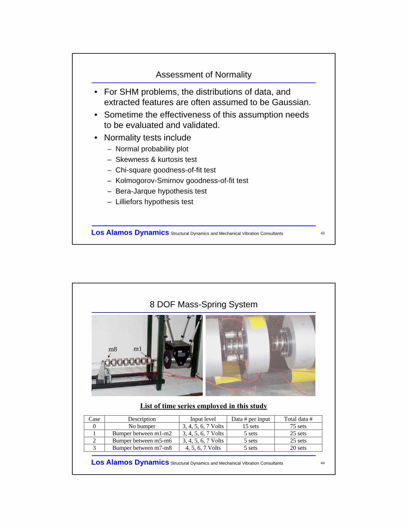
8 DOF Mass-Spring System
Case Description Input level Data # per input Total data #0 No bumper 3, 4, 5, 6, 7 Volts 15 sets 75 sets1 Bumper between m1-m2 3, 4, 5, 6, 7 Volts 5 sets 25 sets2 Bumper between m5-m6 3, 4, 5, 6, 7 Volts 5 sets 25 sets3 Bumper between m7-m8 4, 5, 6, 7 Volts 5 sets 20 sets
List of time series employed in this study
m1m8
Los Alamos Dynamics Structural Dynamics and Mechanical Vibration Consultants 45
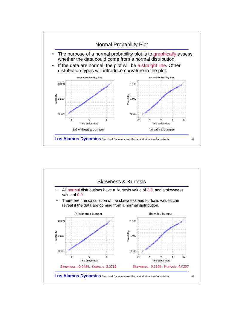
Normal Probability Plot
• The purpose of a normal probability plot is to graphically assess whether the data could come from a normal distribution.
• If the data are normal, the plot will be a straight line. Other distribution types will introduce curvature in the plot.
-5 0 5
0.0010.0030.01 0.02 0.05 0.10 0.25 0.50 0.75 0.90 0.95 0.98 0.99 0.9970.999
Data
Pro
babi
lity
Normal Probability Plot
0.001
0.999
0.500
Time series data
(a) without a bumper
-10 -5 0 5 10
0.0010.0030.01 0.02 0.05 0.10 0.25 0.50 0.75 0.90 0.95 0.98 0.99 0.9970.999
Data
Pro
babi
lity
Normal Probability Plot
0.001
0.999
0.500
Time series data
(b) with a bumper
Los Alamos Dynamics Structural Dynamics and Mechanical Vibration Consultants 46
Skewness & Kurtosis
• All normal distributions have a kurtosis value of 3.0, and a skewness value of 0.0.
• Therefore, the calculation of the skewness and kurtosis values can reveal if the data are coming from a normal distribution.
-5 0 5
0.0010.0030.01 0.02 0.05 0.10 0.25 0.50 0.75 0.90 0.95 0.98 0.99 0.9970.999
Data
Pro
babi
lity
Normal Probability Plot
0.001
0.999
0.500
Time series data
Skewness=-0.0439, Kurtosis=3.0736
(a) without a bumper
-10 -5 0 5 10
0.0010.0030.01 0.02 0.05 0.10 0.25 0.50 0.75 0.90 0.95 0.98 0.99 0.9970.999
Data
Pro
babi
lity
Normal Probability Plot
0.001
0.999
0.500
Time series data
Skewness= 0.3165, Kurtosis=4.0207
(b) with a bumper

Los Alamos Dynamics Structural Dynamics and Mechanical Vibration Consultants 47
Testing Validity of Assumed Distribution
• The previous analyses of the normal probability plot and the estimation of skewness & kurtosis are very easy and convenient, but do not provide principled procedures.
• There are more statistically rigorous tests for verifying the validity of the assumed distribution. These tests are called goodness-of-fit tests.
• The chi-square and Kolmogorov-Smirnov methods are the two most common ones.
Los Alamos Dynamics Structural Dynamics and Mechanical Vibration Consultants 48
Chi-square Test for Distribution
• The relative errors approach the chi-square distribution with f (m-1-k) degrees-of-freedom as the sample size increases infinitely. Where k is the number of distribution parameters estimated from the data
-400 -200 0 200 4000
2000
4000
6000
8000
Num
ber
of s
ampl
es
m
i n
nn
1
2)ˆ(
• The assumed distribution is substantiated by the data with 100 x (1- confidence if the inequality holds.
Assumed theoretical distribution
Histogram from n data points (with m number of bins, based on judgment)
Compute the errors: )ˆ( nn
)%1(100 confidence Interval
Chi-squaredistribution
f 1If usually taken to be between 1% and
Note that more than one distribution can satisfy this test

Los Alamos Dynamics Structural Dynamics and Mechanical Vibration Consultants 49
-4 -2 0 2 40
0 . 2
0 . 4
0 . 6
0 . 8
1
Data
Cu
mu
lativ
e P
rob
ab
ility
Kolmogorov-Smirnov Test for Distribution
• K-S Test compares the empirical and theoretical cumulativedensity functions (CDF).
• Compare with the critical value defined at 100x(1-) confident interval. (The critical value is obtained from a K-S test table.)
nD crD
• IF is less than the critical value the assumed distribution is accepted.
nD crD
|)()(|max xSxFD nx
n
Los Alamos Dynamics Structural Dynamics and Mechanical Vibration Consultants 50
Data Reduction/Compression
• Principal Component Analysis (PCA)• Projection Pursuit Analysis (PPA)• Informative Component Analysis (ICA)• Factor Analysis• Multidimensional Scaling• Clustering
XTXY Tf )(
• Find a projection of the feature space X
such that the dimension of the projected features is less thanthat of the original features.

Los Alamos Dynamics Structural Dynamics and Mechanical Vibration Consultants 51
Principal Component Analysis
x1
xPrincipal component analysis finds an orthogonal projection of original data (red) onto a lower dimensional space (blue line) such that variance of the projected points (green) is maximized
Los Alamos Dynamics Structural Dynamics and Mechanical Vibration Consultants 52
Principal Component Analysis (PCA)
• PCA projects the original variables into uncorrelated orthogonal variables.
• PCA transformation matrix T is obtained by solving the eigenvalue problem of the data’s covariance matrix.
TΛΣT Λ : Eigenvalue matrix containing variance info.
T : Eigenvector (principal component) matrix
)( μXTY T
1x
2x
Original feature space
1y2y
Transformed space
12
Los Alamos Dynamics Structural Dynamics and Mechanical Vibration Consultants 53
Principal Component Process
• PCA provides the optimal linear projection of D dimensional data into an M-dimension subspace where M<D such that variance of the projected data is maximized– Find mean vector and covariance matrix for the
multidimensional data
– Find M eigenvectors of the covariance matrix corresponding to the M largest eigenvalues
– Use those eigenvector to define the linear combinations of the original data
Los Alamos Dynamics Structural Dynamics and Mechanical Vibration Consultants 54
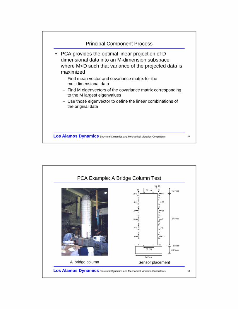
PCA Example: A Bridge Column Test
A bridge column
4
5
6
7
8
9
10
11
12
13
14
15
16
17
18
23
25
24
1
27
26
2
29
28
38
31
30
39
33
32
19
20
2140
35
34
3 22
63.5 cm
3.8 cm
345 cm
45.7 cm
61 cm
142 cm
61 cm
36, 37
Sensor placement
Los Alamos Dynamics Structural Dynamics and Mechanical Vibration Consultants 55
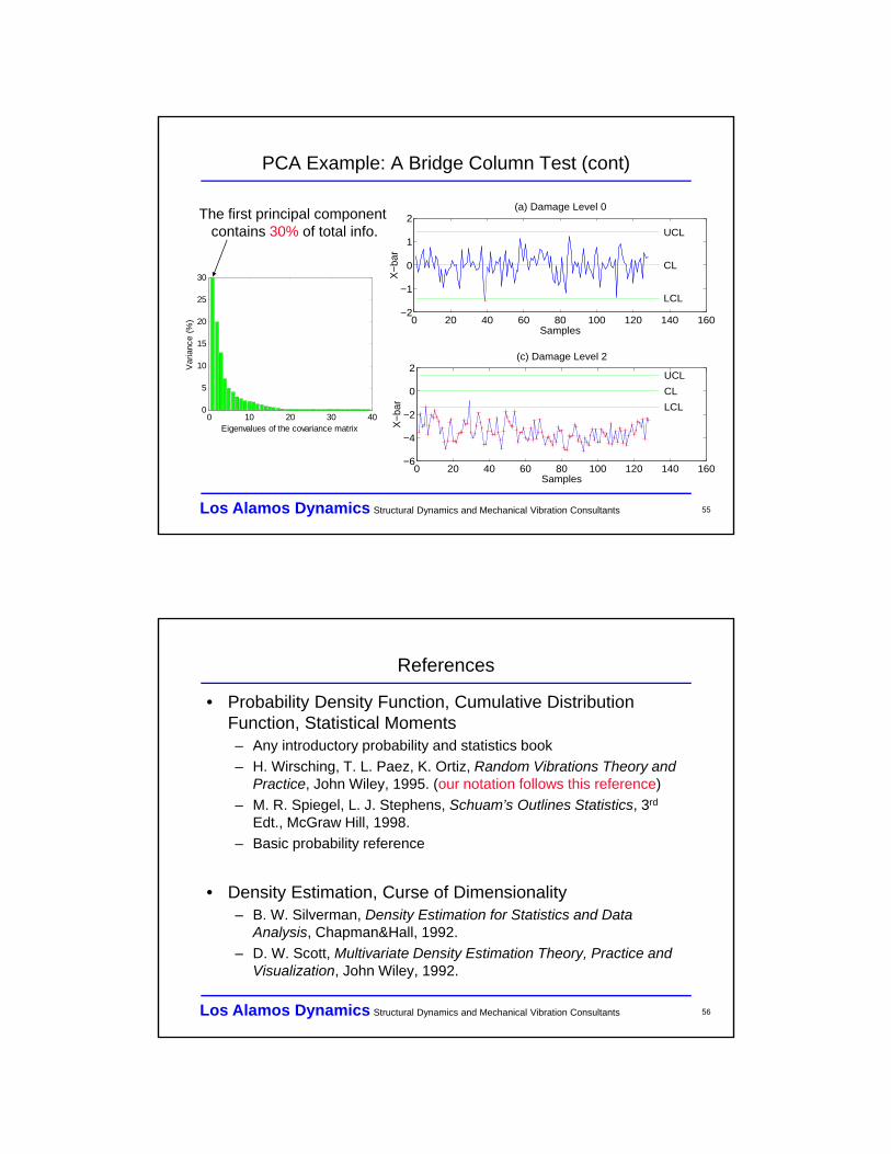
PCA Example: A Bridge Column Test (cont)
0 10 20 30 400
5
10
15
20
25
30
Eigenvalues of the covariance matrix
Var
ianc
e (%
)
ResizeLegend
0 20 40 60 80 100 120 140 160−2
−1
0
1
2UCL
LCL
CL
Samples
X−b
ar
(a) Damage Level 0
0 20 40 60 80 100 120 140 160−6
−4
−2
0
2UCL
LCL
CL
Samples
X−b
ar
(c) Damage Level 2
The first principal component contains 30% of total info.
Los Alamos Dynamics Structural Dynamics and Mechanical Vibration Consultants 56
References
• Probability Density Function, Cumulative Distribution Function, Statistical Moments – Any introductory probability and statistics book
– H. Wirsching, T. L. Paez, K. Ortiz, Random Vibrations Theory and Practice, John Wiley, 1995. (our notation follows this reference)
– M. R. Spiegel, L. J. Stephens, Schuam’s Outlines Statistics, 3rd
Edt., McGraw Hill, 1998.
– Basic probability reference
• Density Estimation, Curse of Dimensionality– B. W. Silverman, Density Estimation for Statistics and Data
Analysis, Chapman&Hall, 1992.
– D. W. Scott, Multivariate Density Estimation Theory, Practice and Visualization, John Wiley, 1992.

Los Alamos Dynamics Structural Dynamics and Mechanical Vibration Consultants 57
References
• Confidence Limits– E. Kreyszig, Advanced Engineering Mathematics, 8th Edt., John
Wiley, 1999.
• Central Limit Theorem, Assessment of Normality– H. Wirsching, T. L. Paez, K. Ortiz, Random Vibrations Theory and
Practice, John Wiley, 1995.)
– A. H-S. Ang and W. H. Tang, Probability Concepts in Engineering Planning and Design: Vol. 1 Basic Principles, 1975.
• Multivariate Analysis, Data Reduction & Compression– W. R. Dillon and M. Goldstein, Multivariate Analysis: Methods and
Applications, 1984.
– D. W. Scott, Multivariate Density Estimation Theory, Practice and Visualization, John Wiley, 1992.
– C. M. Bishop, Neural Networks for Pattern Recognition, Oxford University Press, 1995.