basic statistical concepts and methods for earth scientists · · 2010-02-18basic statistical...
TRANSCRIPT

Basic statistical concepts and methods for earth
scientists
By Ricardo A. Olea
Open-File Report 2008–1017
U.S. Department of the Interior U.S. Geological Survey
[i]

U.S. Department of the Interior KENNETH L. SALAZAR, Secretary
U.S. Geological Survey Marcia K. McNutt, Director
U.S. Geological Survey, Reston, Virginia 2008
For product and ordering information: World Wide Web: http://www.usgs.gov/pubprod Telephone: 1-888-ASK-USGS (1-888-275-8747)
For more information on the USGS—the Federal source for science about the Earth, its natural and living resources, natural hazards, and the environment: World Wide Web: http://www.usgs.gov Telephone: 1-888-ASK-USGS (1-888-275-8747)
Suggested citation: Olea, R.A., 2008, Basic statistical concepts for earth scientists: U.S. Geological Survey, Open-File Report 2008-1017, 191 p.
Revised version, February 2010
Any use of trade, product, or firm names is for descriptive purposes only and does not imply endorsement by the U.S. Government.
Although this report is in the public domain, permission must be secured from the individual copyright owners to reproduce any copyrighted material contained within this report.
[ii]

Basic statistical concepts and methods for earth scientists
Ricardo A. Olea
Open-File Report 2008–1017
U.S. Department of the InteriorU.S. Geological Survey

2
CONTENTS
1. Introduction 32. Data Collection Issues 113. Univariate Statistics 354. Bivariate Statistics 785. Nondetect Statistics 1006. Statistical Testing 1117. Multivariate Statistics 153
These notes have been prepared for teaching a one-day course intended to refresh and upgrade the statistical background of the participants.

3
1. INTRODUCTION

4
STATISTICS
Statistics is the science of collecting, analyzing, interpreting, modeling, and displaying masses of numerical data primarily for the characterization and understanding of incompletely known systems.
Over the years, these objectives have led to a fair amount of analytical work to achieve, substantiate, and guide descriptions and inferences.
5
WHY STATISTICS?• Given any district, time and economics ordinarily
preclude acquiring perfect knowledge of a single attribute of interest, let alone a collection of them, resulting in uncertainty and sometimes into bulky datasets.
• Note that uncertainty is not an intrinsic property of geological systems; it is the result of incomplete knowledge by the observer.
• To a large extent, earth sciences aim to inferring past processes and predicting future events based on relationships among attributes, preferably quantifying uncertainty.Statistics is an important component in the emerging
fields of data mining and geoinformatics.

6
WHEN NOT TO USE STATISTICS?
• There are no measurements for the attribute(s) of interest.
• There are very few observations, say 3 or 4.• The attribute is perfectly known and there is no
interest in having associated summary information, preparing any generalizations, or making any type of quantitative comparisons to other attributes.

7
CALCULATIONS
As shown in this course, most of the statistical calculations for the case of one attribute are fairly trivial, not requiring more than a calculator or reading a table of values.
Multivariate methods can be computationally intensive, suited for computer assistance. Computer programs used to be cumbersome to utilize, some requiring the mastering of special computer languages.
Modern computer programs are easy to employ as they are driven by friendly graphical user interfaces. Calculations and graphical display are performed through direct manipulation of graphical icons.

8
EXAMPLE OF MODERN PROGRAM

9
COURSE OBJECTIVESThis short course is intended to refresh basic concepts and present various tools available for the display and optimal extraction of information from data.
At the end of the course, the participants: • should have increased their ability to read the
statistical literature, particularly those publications listed in the bibliography, thus ending better qualified to independently apply statistics;
• may have learned some more theoretically sound and convincing ways to prepare results;
• might be more aware both of uncertainties commonly associated with geological modeling and of the multiple ways that statistics offers for quantifying such uncertainties.

10
“That’s the gist of what I want to say. Now get me some statistics to base it on.”
©The N
ew Yorker Collection 1977 Joseph Mirachi
from cartoonbank.com
. All rights reserved.

11
2. DATA COLLECTION ISSUES

12
ACCURACY AND PRECISION

13
ACCURACY
Accuracy is a property of measured and calculated quantities that indicates the quality of being close to the actual, true value.• For example, the value 3.2 is a more accurate
πrepresentation of the constant (3.1415926536 …) than 3.2564.
• Accuracy is related to, but not synonymous with precision.

14
PRECISION
In mathematics, precision is the number of significant digits in a numerical value, which may arise from a measurement or as the result of a calculation.
The number 3.14 is less precise representation of πthe constant than the number 3.55745.
For experimentally derived values, precision is related to instrumental resolution, thus to the ability of replicating measurements.

15
ACCURACY AND PRECISION
Mathematically, a calculation or a measurement can be:• Accurate and precise. For
example 3.141592653 is both an accurate and precise value of π.
• Precise but not accurate, like π = 3.5893627002.
• Imprecise and inaccurate, such as π = 4.
• Accurate but imprecise, such as π = 3.1.
Accuracy
Pre
cisi
on
Experimental context
While precision is obvious to assess, accuracy is not. To a large extent, what is behind statistics is an effort to evaluate accuracy.

16
SIGNIFICANT DIGITS
17
SIGNIFICANT DIGITS
Significant digits are the numerals in a number that are supported by the precision of a measurement or calculation.• The precision of a measurement is related to the
discriminating capability of the instrument.• The precision of a calculation is related to the numbers
involved in the arithmetic processing and is decided by a few simple rules.

18
SIGNIFICANT DIGITS IN A NUMBER• Digits from 1-9 are always significant.• Zeros between two other significant digits are always
significant.• Zeros used solely for spacing the decimal point
(placeholders) are not significant. For example, the value 0.00021 has two significant digits.
• Trailing zeros, both to the right of the decimal place and of another significant digit, are significant. For example, 2.30 has three significant digits.
• For real numbers, zeros between the rightmost significant digit and the decimal place are not significant. Hence, 4000.
is automatically understood to have one
significant digit. If, for example, indeed there are two, use the notation 4.0.103.
• Whole numbers have unlimited number of significant digits. So, 4000 has infinite significant digits.

19
SIGNIFICANT DIGITS IN CALCULATIONSReporting results often requires some manual rounding, especially if using calculators or computers.
In all four basic operations of addition, substraction, multiplication, and division, the number with the least significant digits in decimal places determines the significant decimal digits to report in the answer. Examples:
• 2.1 + 2.08 = 4.2• (8.1.2.08)/4 = 4.2
Easy way corollary:If all the operands have the same number of significant decimal places, the significant decimal places in the result are the same as those of the operands. Example: 0.38.27.90 - 4.28/10.25 = 10.18

20
DETECTION LIMIT

21
LIMITS IN CHEMICAL ANALYSESIn analytical chemistry, the detection limit is the lowest
quantity of a substance at which it can be decided whether an analyte is present or not, a problem that arises from the fact that instruments produce readings even in the complete absence of the analyte.
xLThe limit actually measured, , is:xL = xbl + k ⋅sbl
xblwhere is the mean of sbl blank measurements, their standard deviation, and k a reliability factor commonly taken equal to 3. If S is the sensitivity of the calibration curve, then the detection limit, LOD, is:
LOD = k ⋅sbl ⋅S
22
EXAMPLE OF COPPER DETECTION (1)
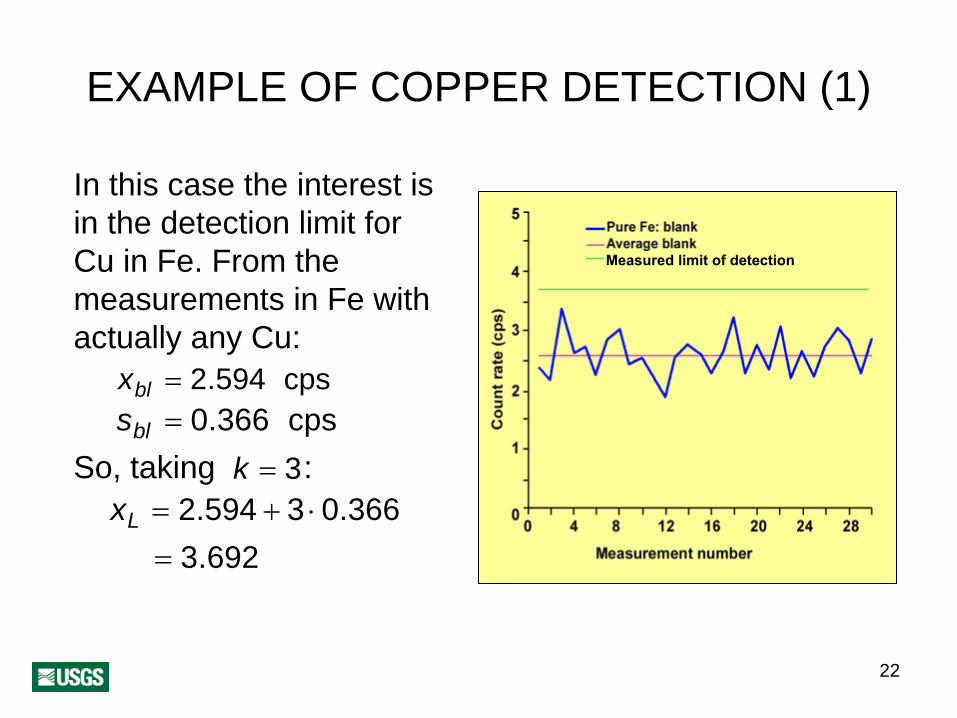
In this case the interest is in the detection limit for Cu in Fe. From the measurements in Fe with actually any Cu:
xbl = 2.594 cpssbl = 0.366 cps
So, taki k = 3ng :xL = 2.594 + 3 ⋅0.366
= 3.692
Measured limit of detection

23
EXAMPLE OF COPPER DETECTION (2)
The sensitivity of the calibration curve, S, is the inverse of the rate of change of instrumental reading with changes in the concentration of the analyte above the detection limit, LOD. In our example,
S = 0.074 %/cps.ThusLOD = 3 ⋅0.366 ⋅0.074
= 0.08 %Cu
2
4
6
8
0 0.1 0.2 0.3 0.4Standard, percent
Mea
sure
d, c
ount
s pe
r sec
ond
24
INSTRUMENTAL DETECTION LIMIT
The Limit of Detection presumes a matrix clean of other interfering substances. In such a case, the Limit of Detection is a special case of Instrumental Detection Limit, IDL:
LOD = IDL .

25
METHOD DETECTION LIMIT
In the presence of complex matrices that can complicate the calculation of the background properties, it is common to use the Method Detection Limit, MDL, instead of simply the Instrumental Detection Limit, IDL.
In the detection of copper, iron is a clean matrix and stainless steel would be a complex matrix with several alloys.
The Method Detection Limit can be anywhere from 2 to 5 times higher than the Instrumental Detection Limit
MDL = (2 to 5)⋅ IDL

26
LIMIT OF QUANTITATION
A common misconception is that the LOD is the minimum concentration that can be measured. Instead, LOD is the concentration at which one can be reasonably certain that the concentration is not zero.
Just because one can tell something from noise does not mean that one can necessarily know how much of the analyte there actually is. Quantitation is generally agreed to start at 5 times the Method Detection Limit. This higher concentration is called Practical Quantitation Limit, PQL. Thus
PQL = 5 ⋅MDL
27
SUMMARY
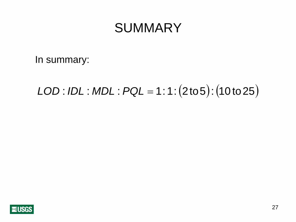
In summary:
LOD : IDL : MDL : PQL = 1:1: 2 to5 : (10( ) to25)

28
LEGACY DATA

29
LEGACY DATA
Legacy data are information in the development of which an organization has invested significant resources in its preparation and that has retained its importance, but that has been created or stored using software and/or hardware that is perceived outmoded or obsolete by current standards.• Working with legacy data is ordinarily a difficult and
frustrating task.• Customarily, legacy data are too valuable to be
ignored.• The nature of problems is almost boundless, yet it is
possible to group them in some general categories.

30
COMMON PROBLEMS WITH LEGACY DATA
• Data quality challenges• Database design problems• Data architecture problems• Processing difficulties

31
TYPICAL DATA QUALITY PROBLEMS
• Different technologies in acquiring the data.• Obsolete methods and conventions were used to
prepare the data.• The purpose of a column in a tabulation is determined by
the value of one or several other columns.• Inconsistent data formatting.• Frequently missing data.• Multiple codes have the same meaning.• Varying default values.• Multiple source for the same type of information.

32
COMMON DATABASE DESIGN PROBLEMS
• Inadequate documentation.• Ineffective or no naming conventions.• Text and numbers appear in the same column.• Original design goals are at odds with current project
needs.

33
COMMON ARCHITECTURE PROBLEMS
• Different hardware platforms.• Different storage devices.• Redundant data sources.• Inaccessible data in obsolete media.• Poor or lacking security.

34
LEGACY DATA EVALUATIONIssues to consider include: • Are the data needed to achieve an established goal? • What will be lost if this information is eliminated? • Are the data consistent? • Are the data accurate and up-to-date? • How much data are missing? • What is the format of the data? • Can the new system support the same format? • Is the information redundant? • Is this information stored in multiple ways or multiple
times?
We are all generating legacy data. Be visionary!
35
3. UNIVARIATE STATISTICS
36
EVERYTHING AND A PIECEIn statistics, population is the collection of all possible outcomes or individuals comprising the complete system of our interest; for example all people in the United States.
Populations may be hard or impossible to analyze exhaustively. In statistics, a limited collection of measurements is called sample; for example, a Gallup Poll.
Unfortunately, the term “sample” is employed with different meanings in geology and statistics.
Geology Statistics collection sample sample observation
The statistical usage of the term sample is observed in what follows.

37
RANDOM VARIABLE
• A random variable or variate is a quantity that may take any of the values within a given set with specified relative frequencies.
• The concept is heavily utilized in statistics to characterize a population or convey the unknown value that an attribute may take.
Variate
Freq
uenc
y

38
DESCRIPTIVE ANALYSIS
• A sample of an attribute ordinarily comprises several measurements, which are best understood when organized in some way, which is an important aspect of statistics.
• The number of measurements in a sample is the sample size.
• There are multiple options to make the data more intelligible, some more convenient than others, depending on factors such as the sample size and the ultimate objectives of the study.
39
SAMPLE VISUALIZATION

40
FREQUENCY TABLE
Given some numerical information, if the interval of variation of the data is divided into class intervals— customarily of the same lengths—and all observations are assigned to their corresponding classes, the result is a count of relative frequency of the classes.
41
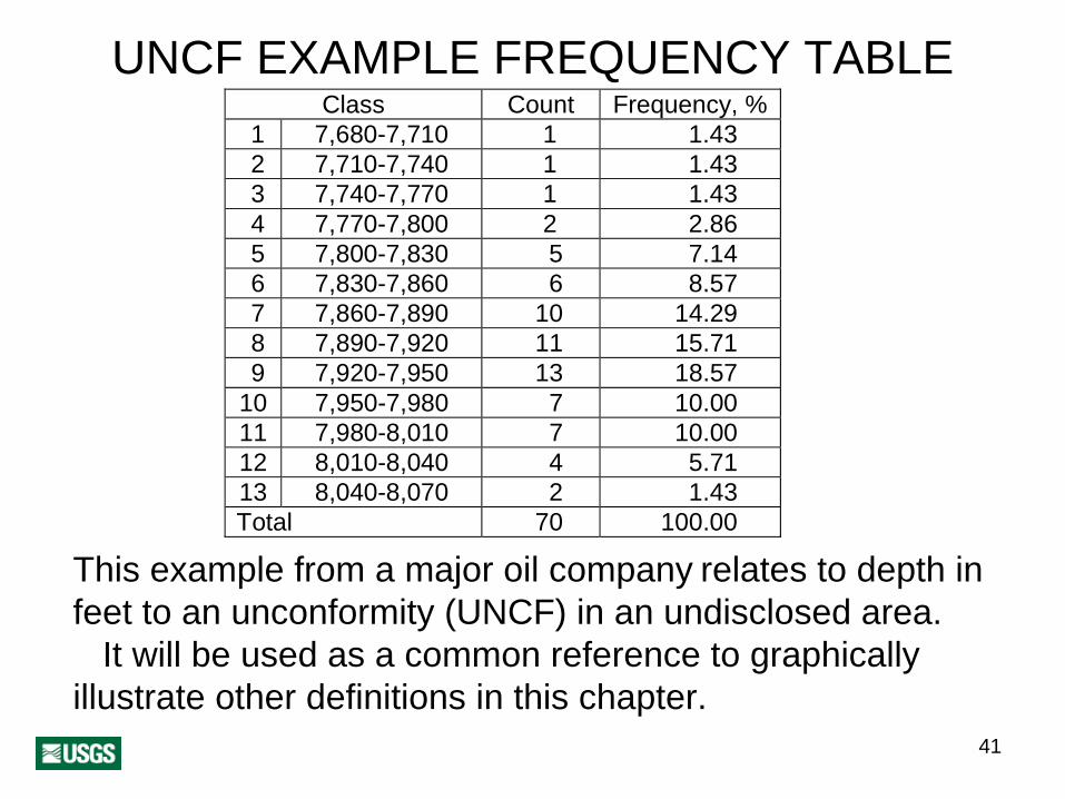
UNCF EXAMPLE FREQUENCY TABLEClass Count Frequency, %
1 7,680-7,710 1 1.43 2 7,710-7,740 1 1.43 3 7,740-7,770 1 1.43 4 7,770-7,800 2 2.86 5 7,800-7,830 5 7.14 6 7,830-7,860 6 8.57 7 7,860-7,890 10 14.29 8 7,890-7,920 11 15.71 9 7,920-7,950 13 18.57
10 7,950-7,980 7 10.00 11 7,980-8,010 7 10.00 12 8,010-8,040 4 5.71 13 8,040-8,070 2 1.43 Total 70 100.00
This example from a major oil company relates to depth in feet to an unconformity (UNCF) in an undisclosed area.
It will be used as a common reference to graphically illustrate other definitions in this chapter.

42
HISTOGRAM
0
4
8
12
16
20
7695 7755 7815 7875 7935 7995 8055
Depth, ft
Freq
uenc
y, p
erce
nt
A histogram is a graphical representation of a frequency table.

43
CUMULATIVE FREQUENCYSummaries based on frequency tables depend on the selection of the class interval and origin.
Given a sample of size n, this drawback is eliminated by displaying each observation zi versus the proportion of the sample that is not larger than zi .
Each proportion is a multiple of 100/n. The vertical axis is divided in n intervals and the data are displayed at the center of the corresponding interval.
Customarily, the vertical axis is scaled so that data from a normal distribution (page 69) display as a straight line.

44
SUMMARY STATISTICS

45
SUMMARY STATISTICSSummary statistics are another alternative to histograms and cumulative distributions.
A statistic is a synoptic value calculated from a sample of observations, which is usually but not necessarily an estimator of some population parameter.
Generally, summary statistics are subdivided into three categories:• Measures of location or centrality• Measures of dispersion• Measures of shape
46
MEASURES OF LOCATION
Measures of location give an idea about the central tendency of the data. They are: • mean• median• mode
47
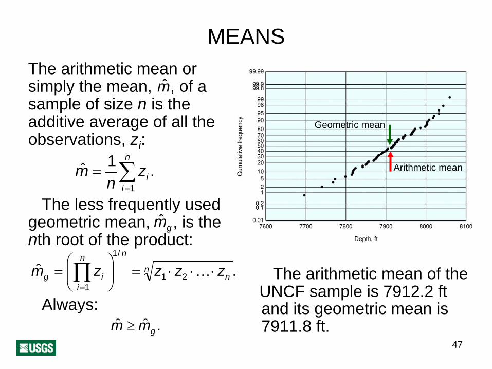
MEANSThe arithmetic mean or
msimply the mean, , of a sample of size n is the additive average of all the observations, zi :
1 n
m = ∑zi .n i=1
The less frequently used mggeometric mean, , is the
nth root of the product:⎛ ⎞
1/ nn
m = ⎜ ⎟ ng ∏zi = z1 ⋅ z2 ⋅K ⋅⎜ ⎟ zn .
⎝ i=1 ⎠Always:
m ≥ mg .
Geometric mean
Arithmetic mean
The arithmetic mean of the UNCF sample is 7912.2 ft and its geometric mean is 7911.8 ft.

48
THE MEDIANThe median, Q2 , of a sample is the value that evenly splits the number of observations zi into a lower half of smallest observations and the upper half of largest measurements.
If zi is sorted by increasing values, then
⎪⎧z n 1 / 2,( ) if is odd,Q + n
2 = ⎨⎪ ⋅ +⎩0.5 zn / 2 z n / 2 +1( ) , if n is even( ) .
he median of the UNCF sample is 7918 ft.T
Median

49
THE MODE
0
4
8
12
16
20
7695 7755 7815 7875 7935 7995 8055
Depth, ft
Freq
uenc
y, p
erce
nt
Mode The mode of a sample is the most probable or frequent value, or equivalently, the center point of the class containing the most observations.
For the UNCF sample, the center of the class with the most observations is 7935 ft.

50
ROBUSTNESS
Robustness denotes the ability of statistical methods to work well not only under ideal conditions, but in the presence of data problems, mild to moderate departures from assumptions, or both.
For example, in the presence of large errors, the median is a more robust statistic than the mean.

51
MEASURES OF SPREAD
Measures of spread provide an idea of the dispersion of the data. The most common measures are:• variance• standard deviation• extreme values• quantiles• interquartile range
52
VARIANCE
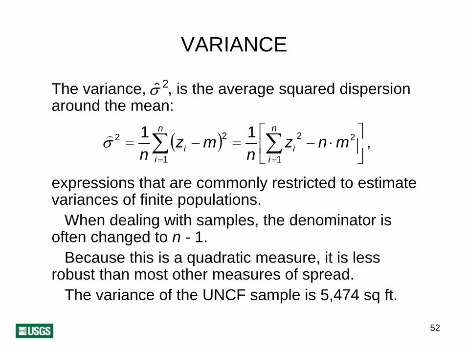
The variance, σ 2, is the average squared dispersion around the mean:
( ) ,11 2
1
2
1
22⎥⎦
⎤⎢⎣
⎡⋅−=−= ∑∑
==
mnzn
mzn
n
ii
n
iiσ)
expressions that are commonly restricted to estimate variances of finite populations.
When dealing with samples, the denominator is often changed to n - 1.
Because this is a quadratic measure, it is less robust than most other measures of spread.
The variance of the UNCF sample is 5,474 sq ft.

53
STANDARD DEVIATION The standard deviation isthe positive square root of the variance.
It has the advantage ofbeing in the same units as the attribute.
The standard deviationof the UNCF sample is 74.5 ft.
σσσ σ
t >1theorem, for any sample and , the proportion of data mthat deviates from the mean at t ⋅σ t −2least is at most :
( ) 1Prop X − m ≥ t ⋅σ ≤ 2t
According to Chebyshev’s

54
EXTREME VALUES
The extreme values are the minimum and the maximum.
For the UNCF sample, the minimum value is 7,696 ft and the maximum value is 8,059 ft.This measure is not particularly robust, especially for small samples.

55
QUANTILES
The idea of the median splitting the ranked sample into two equal-size halves can be generalized to any number of partitions with equal number of observations. The partition boundaries are called quantiles or fractiles. The names for the boundaries for the most common quantiles are:• Median, for 2 partitions• Quartiles, for 4 partitions• Deciles, for 10 partitions• Percentiles, for 100 partitionsThere is always one less boundary than the number of partitions.
56
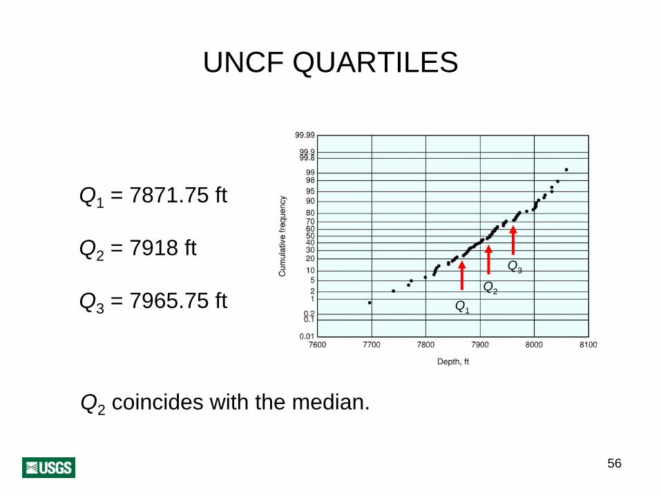
UNCF QUARTILES
Q1 = 7871.75 ft
Q2 = 7918 ft
Q3 = 7965.75 ftQ2
Q1
Q3
Q2 coincides with the median.
57
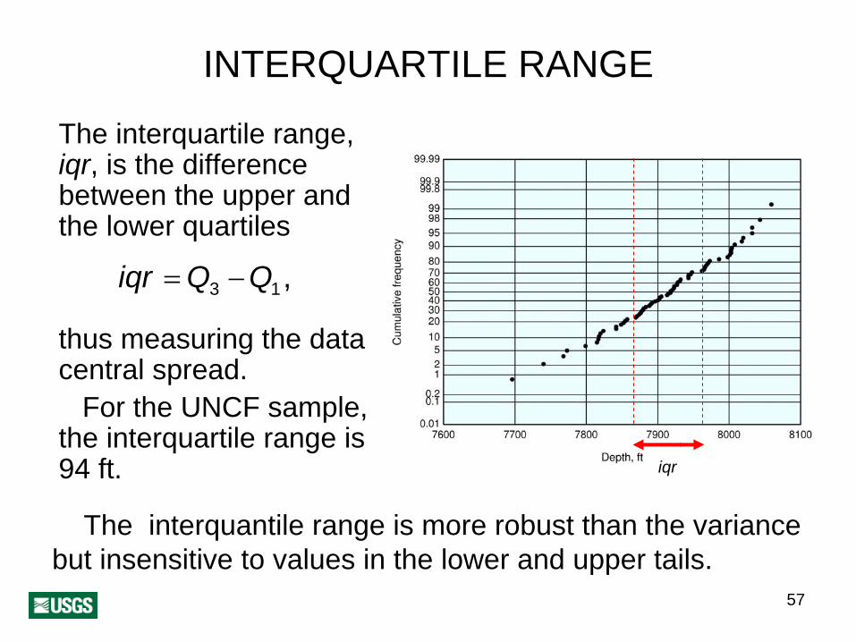
INTERQUARTILE RANGE
The interquartile range, iqr, is the difference between the upper and the lower quartiles
iqr =Q3 −Q1,
thus measuring the data central spread.
For the UNCF sample, the interquartile range is 94 ft. iqr
The interquantile range is more robust than the variance but insensitive to values in the lower and upper tails.

58
OUTLIEROutliers are values so markedly different from the rest of the sample that they rise the suspicion that they may be from a different population or that they may be in error, doubts that frequently are hard to clarify. In any sample, outliers are always few, if any.
A practical rule of thumb is to regard any value deviating more than 1.5 times the interquartile range, iqr, from the median as a mild outlier and a value departing more than 3 times iqr as an extreme outlier.
0
4
8
12
16
20
7695
7755
7815
7875
7935
7995
8055
8115
8175
8235
Depth, ft
Freq
uenc
y, p
erce
nt
mild
extre
me
3iqr
mild
1.5iqr
For the UNCF sample, all mild outliers seem to be legitimate values, while the extreme outlier of 8,240 ft is an error.

59
BOX-AND-WHISKER PLOTThe box-and whisker plot is a simple graphical way to summarize several of the statistics:• Minimum• Quartiles• Maximum• Mean
Variations of this presentation abound. Extremes may exclude outliers, in which case the outliers are individually posted as open circles. Extremes sometimes are replaced by the 5 and 95 percentiles.
7600
7700
7800
7900
8000
8100
Dep
th, f
t
Max.
Min.
Q1
Q2
Q3
UNCF
+Mean

60
MEASURES OF SHAPE
The most commonly used measures of shape in the distribution of values are:• Coefficient of skewness• Quartile skew coefficient• Coefficient of kurtosis

61
COEFFICIENT OF SKEWNESS
The coefficient of skewness is a measure of asymmetry of the histogram. It is given by:
( )3
1
3
1
1
σ
∑=
−
=
n
ii mz
nB
B1 < 0If : , the left tail is longer;
B1 = 0, the distribution is symmetric;
B1 > 0, the right tail is longer.
0
4
8
12
16
20
7695 7755 7815 7875 7935 7995 8055
Depth, ft
Freq
uenc
y, p
erce
nt
B1 = -0.38
The UNCF coefficient of skewness is -0.38.
62
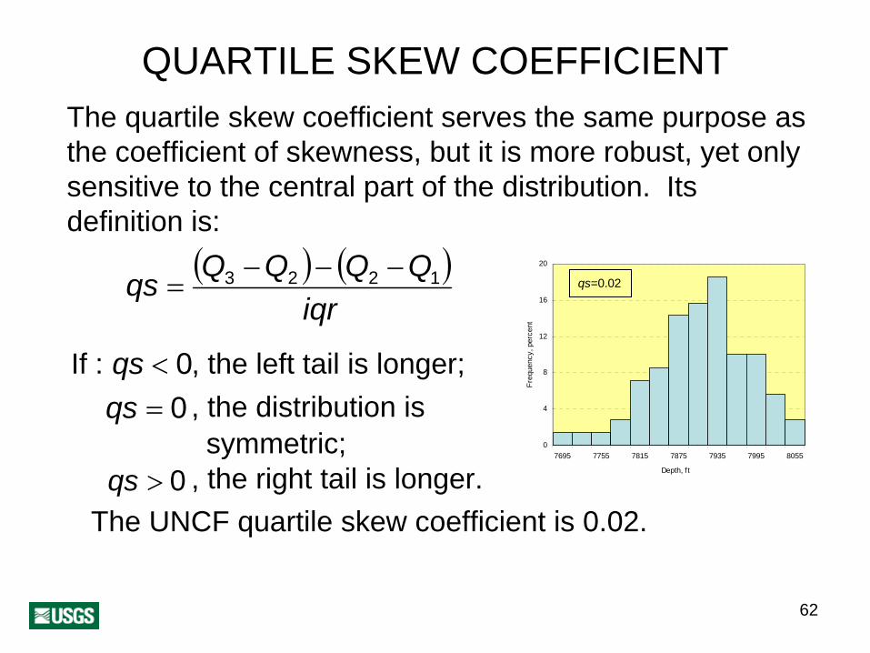
QUARTILE SKEW COEFFICIENTThe quartile skew coefficient serves the same purpose as the coefficient of skewness, but it is more robust, yet only sensitive to the central part of the distribution. Its definition is:
( ) )Q Q (Q Qqs 3 − 2 − 2 −= 1
iqr
qs < 0If : , the left tail is longer;qs = 0 , the distribution is
symmetric;qs > 0 , the right tail is longer.
0
4
8
12
16
20
7695 7755 7815 7875 7935 7995 8055
Depth, ft
Freq
uenc
y, p
erce
nt
qs=0.02
The UNCF quartile skew coefficient is 0.02.
63
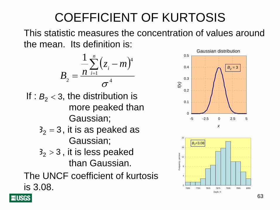
COEFFICIENT OF KURTOSISThis statistic measures the concentration of values around the mean. Its definition is:
( )4
1
4
2
1
σ
∑=
−=
n
ii mz
nB
0
0.1
0.2
0.3
0.4
0.5
-5 -2.5 0 2.5 5
x
f(x)
Gaussian distribution
B2 = 3
B2 < 3If : , the distribution is more peaked than Gaussian;
B2 = 3, it is as peaked as Gaussian;
B2 > 3 , it is less peaked than Gaussian.
The UNCF coefficient of kurtosis is 3.08.
0
4
8
12
16
20
7695 7755 7815 7875 7935 7995 8055
Depth, f t
Freq
uenc
y, p
erce
nt
B2 =3.08

64
MODELS

65
PROBABILITYProbability is a measure of the likelihood that an event, A, may occur. It is commonly denoted by Pr[A].
• The probability of an impossible event is zero, Pr[A] = 0. It is the lowest possible probability.
• The maximum probability is Pr[A] = 1, which denotes certainty.
• When two events A and B cannot take place simultaneously, Pr[A or B] = Pr[A] + Pr[B].
• Frequentists claim that Pr[A] = NA /N, where N is total number of outcomes and NA the number of outcomes of A. The outcomes can be counted theoretically or experimentally.
• For others, a probability is a degree of belief in A, even if no random process is involved nor a count is possible.
66
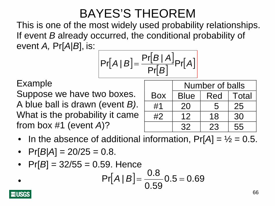
BAYES’S THEOREMThis is one of the most widely used probability relationships. If event B already occurred, the conditional probability of event A, Pr[A|B], is:
[ ] Pr[B | A]Pr A | B = [ ][ ] Pr APr B
ExampleSuppose we have two boxes. A blue ball is drawn (event B). What is the probability it came from box #1 (event A)?
Box Number of balls
Blue Red Total#1 20 5 25 #2 12 18 30
32 23 55 • In the absence of additional information, Pr[A] = ½ = 0.5.• Pr[B|A] = 20/25 = 0.8. • Pr[B] = 32/55 = 0.59. Hence
0.8• Pr A | B =[ ] 0.5 = 0.69
0.59

67
PROBABILITY FUNCTIONSAnalytical functions approximating experimental fluctuations are the alternative to numerical descriptors and measures. They provide approximations to general conditions. The drawback is loss of fine details in favor of simpler models.
Analytical expressions approximating histograms are called probability density functions; those modeling cumulative frequencies are the cumulative distribution functions.
Variations in the parameters in an expression allow the generation of a family of functions, sometimes with radically different shapes.
Main subdivision is into discrete and continuous functions, of which the binomial and normal distribution, respectively, are two typical and common examples.

68
BINOMIAL DISTRIBUTIONThis is the discrete probability density function, f x;p,n( ). , of the number of successes in a series of independent (Bernoulli) trials, such as head or tails in coin flipping. If the probability of success at every trial is p, the probability of x successes in n independent trials is
f (x ; 0.5, 12)
0
0.1
0.2
0.3
Number of successes
Pro
babi
lity
0 1 2 3 4 5 6 7 8 9 10 11 12
0.4
n!
f (x ; 0.1, 12)
0
0.1
0.2
0.3
Number of successes
Pro
babi
lity
0 4 5321 6 7 8 1211109
0.4
f x;p,n =( ) px 1− p n−x ,( )( ) x = 0,1, 2,K, nx! n − x !

69
NORMAL DISTRIBUTION
0
0.1
0.2
0.3
0.4
0.5
-5 -2.5 0 2.5 5
x
f(x; 0
,1)
The most versatile of all continuous models is the normal distribution, also known as Gaussian distribution. Its parameters are μ and σ, which coincide with the mean and the standard deviation.
( ) =xf ,; σμ( )
∞<<∞−−
−xe
x
,2
1 2
2
2σμ
πσ
If X = log(Y) is normally distributed, Y is said to follow a lognormal distribution. Lognormal distributions are positively defined and positively skewed.

70
PROBABILITY FROM MODELSx
X ≤ x = ∫1
Prob 1 f[ ] x( )dx Prob[X ≤ x1] = F (x1)−∞ Examples:
1.17
Prob X ≤ 1.17 = ∫[ ] Normal x;0,1 dx( ) Prob[X ≤ 1.17] = F (1.17)−∞ = 0.88
= 0.88

71
EXPECTED VALUE
Let X be a random variable having a probability f (x)distribution , and let u(x) be a function of x.
u(x)The expected value of is denoted by the E u(x)[ ]operator and it is the probability weighted
average value of u(x).Continuous case, such as temperature:
[ ]( ) ∫∞
E u x = u x f−∞
( ) x( )dxDiscrete case, like coin flipping:
E[u(x)] = ∑u(x f) (x)x

72
EXAMPLE
For the trivial case
u(x) = x
in the discrete case, if all values are equally probable, the expected value turns into
[ ] ∑=x
xn
xE
which is exactly the definition of the mean.
1

73
MOMENT
Moment is the name given to the expected value when the function of the random variable, if it exists,
(x − a)ktakes the form , where k is an integer larger than zero, called the order.
If a is the mean, then the moment is a central moment.
The central moment of order 2 is the variance. For an equally probable discrete case,
( )∑=
−==n
ii mx
nM
1
222
1σ)

74
SIMULATION

75
SIMULATIONReality is often too complex to be able to analytically derive probabilities as in flipping coins. Modern approaches use computers to model a system and observe it repeatedly, with each repetition being the equivalent of flipping a coin.• Relevant attributes take the form of random variables
instead of being deterministic variables.• Generators of random sequences of numbers between
0-1 play an important part in simulation.• The other important component is
the Monte Carlo method, which allows drawing values from the distributions.
• The final result is the histogram(s) for the output variable(s).
00.10.20.30.40.50.60.70.80.9
11.1
Attribute
Cum
ulat
ive
prob
abili
tyxmin xmax

76
BOOTSTRAP• This is a resampling form of the
Monte Carlo method for the numerical modeling of distributions.
• It works directly with the sample instead of its distribution.
• In its simplest form, the general steps are:1. Randomly pick as many
measurements as the sample size. Some values may be taken more than once, while others not at all.
2. Calculate and save as many statistics as interested.
3. Go back to step 1 and repeat the process at least 1,000 times.

77
Moore and N
otz, 2006

78
4. BIVARIATE STATISTICS

79
TOOLS
Frequently there is interest in comparing two or more measurements made for the same object or site. Among the most common alternatives, we have:• Scatterplot• Correlation coefficient• Regression• Quantile-Quantile plot• Probability-Probability plot
Some of these concepts can be generalized to more than two variables, and all multivariate techniques in Chapter 7 are valid for two variables.

SCATTERPLOTSA bivariate scatterplot is a Cartesian posting in which the abscissa and the ordinate are any two variables consistently measured for a series of objects.
Scatterplots are prepared for exploring or revealing form, direction, and strength of association between two attributes.
80
Mecklenburg Bay seafloor, Germany
81
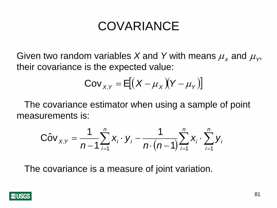
COVARIANCE
Given two random variables X and Y μx μYwith means and , their covariance is the expected value:
( )( )[ YXYX YX μμ −−=ECov ,
The covariance estimator when using a sample of point measurements is:
( ) ∑∑∑===
⋅−⋅
−⋅−
=n
ii
n
ii
n
iiiYX yx
nnyx
n 111, 1
11
1voC
The covariance is a measure of joint variation.
]

82
CORRELATION COEFFICIENTThis coefficient is the number most commonly used to summarize bivariate
σ Xcomparisons. If σYand are the standard deviations for two variables, their correlation coefficient, ρ, is given by:
YX
YX
σσρ
⋅= ,Cov
• It only makes sense to employ ρ for assessing linear associations.
• ρ varies continuously from -1 to 1:1, perfect direct linear correlation 0, no linear correlation-1, perfectly inverse correlation
-0.5
-1
0
1

83
SENSITIVITY TO OUTLIERS
Moore and N
otz, 2006

84
REGRESSIONRegression is a method for establishing analytical dependency of one or more variables on another mainly to determine the degree of their dependency, to estimate values not included in the sampling, or to summarize the sampling.• The variable in the abscissa is called the
regressor, independent, or explanatory variable.• The variable in the ordinate is the regressed,
dependent, or response variable.• In many studies, which variable goes into which
axis is an arbitrary decision, but the result is different. Causality or the physics of the process may help in solving the indetermination.

85
REGRESSION MODEL
Explanatory variable (x)
Res
pons
e va
riabl
e (y
)
εi
( )θ;ixf
• The model is:yi = f (xi ;θ)+ ε i
• f (xi ;θ) is any continuous function of x that is judiciously
θselected by the user. are unknown parameters.
• εTerm is a random variable accounting for the error.
• f (xi ;θ)Having selected , θparameters are calculated
by minimizing total error, for which there are several methods.
Avoid using the model outside the sample range of the explanatory variable.

86
LINEAR REGRESSION
The simplest case is linear regression with parameters obtained minimizing the mean square error, MSE :
Mecklenburg Bay seafloor, Germany
ρ = 0.94
∑=
=n
iiE n
MS1
21 ε
In this special situation, ρ 2
accounts for the proportion of variation accounted by the model.
In the example, ρ = 0.94. Hence, in this case, the (linear regression explains 88% 100 ⋅ ρ 2 ) of the variation.

87
NONLINEAR REGRESSION
MSE = 25.47
Linear
MSE = 20.56
Quadratic polynomial
• In theory, the higher the polynomial degree, the better the fit.
• In practice, the higher the polynomial, the less robust the solution.
• Overfitting may capture noise and not systematic variation.
Cubic polynomial
MSE = 20.33
Sixth degree polynomial
MSE = 19.98

88
IMPLICATIONS
Countries with population over20 million in 1990
50
55
60
65
70
75
80
1 10 100 1000
Persons per television set
Life
exp
ecta
ncy,
yea
r
= -0.81ρ
High to good correlation:• allows prediction of one
variable when only the other is known, but the inference may be inaccurate, particularly if the correlation coefficient is low;
• means the variables are related, but the association may be caused by a common link to a third lurking variable, making the relationship meaningless;
• does not necessarily imply cause-and-effect.

89
After M
oore and Notz, 2006
“In a new effort to increase third-world life ex-pectancy, aid organizations today began delivery of 100,000 television sets.”

90
QUANTILE-QUANTILE PLOT• A quantile-quantile or Q-Q plot is a
scatterplot based on ranked data.• The paring is independent from the
object or site where the observations were taken. The first pair of coordinates has the minimum value for each attribute, the second pair is made of the second smallest readings, and so on until finishing with the two maximum values. Interpolations are necessary for different size samples.
• Identical distributions generate a straight line along the main diagonal.
• Q-Q plots are sensitive to a shift and scaling of the distributions.

91
STANDARDIZED VARIATE
If X is a random variable with mean μ and standard deviation σ, the standardized variate, Z, is the transformation:
σμ−
=XZ
σμ−
=XZ
A standardized variate always has a mean of zero and variance of one.
A standardized Gaussian distribution is called a standard normal distribution. It is often denoted by N(0,1).

92
PROBABILITY-PROBABILITY (P-P) PLOT
DensityVelocity
A P-P plot is another scatterplot prepared by extracting information from the cumulative distributions of two variates.• If the variates are in different units, preliminary
standardization is necessary.• For given thresholds, the axes show the cumulative
probabilities for the two distributions being compared.

93
SPECIAL TOPICS

94
PROPAGATION OF ERRORS
Error propagation is a ratherarchaic term referring to the influence that uncertainty invariables have on a functionof them.
• Under certain simple conditions, it is possible to analytically express the impact of variable uncertainty on the function uncertainty.
• Today the situation is resolved through numerical simulation.
Analytically:N(30,5) = N(12,3) + N(18,4)
Monte Carlo simulation:
f(x)
N(12,3)
0
0.1
0.2
0.3
0.4
0 3 6 9 12 15 18 21 24x
f(x)
0.5N(18,4)
0
0.1
0.2
0.3
0.4
0.5
0 6 12 18 24 30 36x

95
BIAS
Bias in sampling denotes preference in taking the measurements.
Bias in an estimator implies that the calculations are preferentially loaded in one direction relative to the true value, either systematically too high or too low.• When undetected or not compensated, bias induces
erroneous results.• The opposite of the quality of being biased is to be
unbiased.
96
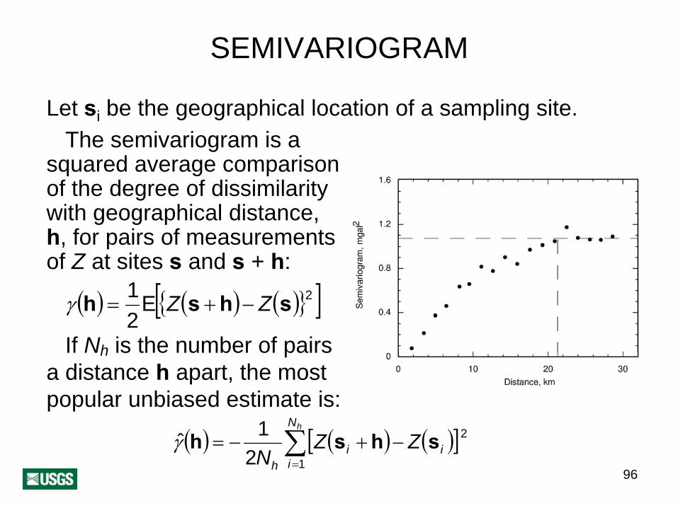
SEMIVARIOGRAM
Let si be the geographical location of a sampling site. The semivariogram is a
squared average comparisonof the degree of dissimilarity with geographical distance, h, for pairs of measurementsof Z at sites s and s + h:
)}[ ]
( ) ( ) ({ 2E21 shsh ZZ −+=γ
If Nh is the number of pairs a distance h apart, the most popular unbiased estimate is:
( ) ( ) ([∑=
−+−=hN
iii ZZ
N 1
2
21ˆ shshγ )]
h
97
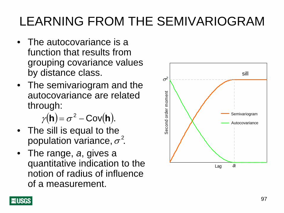
LEARNING FROM THE SEMIVARIOGRAM• The autocovariance is a
function that results from grouping covariance values by distance class.
• The semivariogram and the autocovariance are related through:
γ h( ) = σ 2 −Cov(h).• The sill is equal to the
σ 2population variance, . • The range, a, gives a
quantitative indication to the notion of radius of influence of a measurement.
LagS
econ
d or
der m
omen
t
Semivariogram
Covariance
sill
a
σ2
Autocovariance
Semivariogram
98
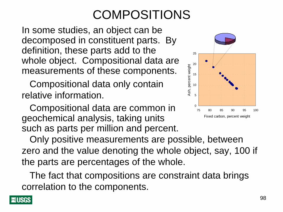
COMPOSITIONSIn some studies, an object can be decomposed in constituent parts. By definition, these parts add to the whole object. Compositional data are measurements of these components.
Compositional data only contain relative information.
Compositional data are common in geochemical analysis, taking units such as parts per million and percent.
Only positive measurements are possible, between zero and the value denoting the whole object, say, 100 if the parts are percentages of the whole.
The fact that compositions are constraint data brings correlation to the components.
0
5
10
15
20
25
75 80 85 90 95 100
Fixed carbon, percent weight
Ash
, per
cent
wei
ght

99
CAUTIONIn general, straight application of statistics to data adding to a constant produces suboptimal or inconsistent results. Most successful ad hoc developments still employ classical statistics, but after taking special precautions.
The most common approach is to transform the data. One possibility is the isometric log-ratio transformation, Y, which for two components, X1 and X2 , is:
cXXXXY
XXY =+== 21
1
2
2
1 with,log21orlog
21
where c is a known closure constant. This transformation:• (−∞,∞)brings the range of variation to ;• eliminates the correlation due to closure;• properly handles distances in attribute space.Results require backtransformation.

100
5. NONDETECT STATISTICS
101
STATISTICS OF THE UNDETECTED
• Undetected values have peculiar characteristics that put them apart from those actually measured.
• Values below detection limit require different treatment than precise measurements.
• There have been several attempts to analyze samples with values below detection limit.

102
STATISTICAL METHODS
The main approaches for the calculation of summary statistics are:• Replacement of the values below detection by an
arbitrary number.• Maximum likelihood method• Kaplan-Meier method• Bootstrap

103
REPLACEMENT
• This is the prevailing practice.• This is not really a method. It has poor to no
justification.• It can lead to completely wrong results.• The most common practice is to replace the values
below detection by half that value.

104
MAXIMUM LIKELIHOOD METHOD THE GENERAL CASE
This is a method for the inference of parameters, θ, of a parent probability density function f (x | θ) based on multiple outcomes, xi .
L(θ) = f (The function x1,K,xn |θ1, K,θm ) is called the likelihood function.
Given outcomes x θ, the optimal parameters are those L(θ) i
that maximize , which come from solving ∂L(θ)/ ∂θ = 0.For example, for the normal distribution,
( ) 22
11
22
221 θ
πθ ⎟⎟⎞
⎜⎜⎛
==− i
i
eL θ( )( )
22
21
21| θθ
θπ
−−
=x
exf θ
the solution is:
( ) 2
1
222
11 ˆˆ1ˆ1 σμθμθ =−=== ∑∑
==
n
ii
n
ii x
nx
n
( )2
2
θ∑
⎠⎝
−n
xn
22
0
0.1
0.2
0.3
0.4
0.5
-5 -2.5 0 2.5 5
x
f(x)
x
f(x|θ
)

105
MAXIMUM LIKELIHOOD OF THE UNDETECTED
• The method is parametric: it requires assuming the distribution that the data would have followed in case all values would have been accurately measured.
• Essential for the success of the method is the assumption of the correct distribution.
• Most commonly selected models are the normal and the lognormal distributions.
• It is commonly used to estimate mean, variance, and quartiles.
• The method tends to outperform the others for samples of size larger than 50, or when 50 to 80% of the values are below detection limit.

106
ARSENIC CONCENTRATION, MANOA STREAM, OAHU,
HAWAII
Mean: 0.945St. dev.: 0.656

107
KAPLAN-MEIER METHOD
• The Kaplan-Meier method works in terms of a survival function, a name derived from clinical applications in which the interest is on survival time after starting medical treatment.
• The Kaplan-Meier method was developed for right censored data—exact measurements are missing above certain values. Left censored data must be flipped using a convenient but arbitrary threshold larger than the maximum.
• Calculated parameters must be backtransformed.• The Kaplan-Meier method tends to work better when
there are more exact measurements than data below detection limit.

108
OAHU DATA SURVIVAL FUNCTION
Flipping constant: 5 micro g/L
0
0.2
0.4
0.6
0.8
1
0 1 2 3 4 5Flipped concentration, micro g/L
Surv
ival
pro
babi
lity
Mean: 0.949St. dev.: 0.807
109
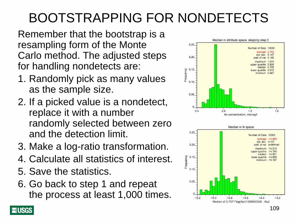
BOOTSTRAPPING FOR NONDETECTSRemember that the bootstrap is a resampling form of the Monte Carlo method. The adjusted steps for handling nondetects are:1. Randomly pick as many values
as the sample size.2. If a picked value is a nondetect,
replace it with a number randomly selected between zero and the detection limit.
3. Make a log-ratio transformation.4. Calculate all statistics of interest.5. Save the statistics.6. Go back to step 1 and repeat
the process at least 1,000 times.

110
COMPARISON OF THE FOUR METHODS EXAMPLE FROM OAHU, HAWAII
Mean St. dev. Q1 Median Q3 μg/L Substituting with zero 0.567 0.895 0.0 0.0 0.7 Subs. half detection lim. 1.002 0.699 0.5 0.95 1.0 Subs. with detection lim. 1.438 0.761 0.75 1.25 2.0
Lognormal Max. Likelihd. 0.945 0.656 0.509 0.777 1.185
Kaplan-Meier, nonparm. 0.949 0.807 0.5 0.7 0.9
Bootstrap average 1.002 0.741 0.501 0.752 1.370 Log-ratio bootstrap aver. 0.938 0.729 0.492 0.738 1.330

111
6. STATISTICAL TESTING
112
STATISTICAL TESTINGThe classical way to make statistical comparisons is to prepare a statement about a fact for which it is possible to calculate its probability of occurrence. This statement is the null hypothesis and its counterpart is the alternative hypothesis.
The null hypothesis is traditionally written as H0 and the alternative hypothesis as H1 .
A statistical test measures the experimental strength of evidence against the null hypothesis.
Curiously, depending on the risks at stake, the null hypothesis is often the reverse of what the experimenter actually believes for tactical reasons that we will examine.

113
EXAMPLES OF HYPOTHESESμ1 μ2Let and be the means of two samples. If one
wants to investigate the likelihood that their means are the same, then the null hypothesis is:
: μμ =Hand the alternative hypothesis is:
: μμ ≠Hbut it could also be:
211 : μμ >HThe first example of H1 is said to be two-sided or two-
μ1 >tailed because includes both μ2 μ1 < μ2 and . The second is said to be one-sided or one-tailed.
The number of sides has implications on how to formulate the test.
210
211
114
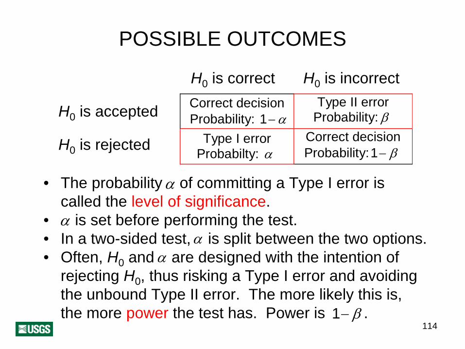
POSSIBLE OUTCOMES
H0 is correct H0 is incorrect
H0 is accepted
H0 is rejected
Correct decision Probability: 1−α
Type II error Probability: β
Type I error Probabilty: α
Correct decision Probability:1− β
• αThe probability of committing a Type I error is called the level of significance.
• α is set before performing the test.• αIn a two-sided test, is split between the two options.• Often, H0 αand are designed with the intention of
rejecting H0 , thus risking a Type I error and avoiding the unbound Type II error. The more likely this is, the more power 1− βthe test has. Power is .

115
IMPORTANCE OF CHOOSING H0Selection of what is null and what is alternative hypothesis has consequences in the decision making. Customarily, tests operate on the left column of the contingency table and the harder to analyze right column remains unchecked. Consider environmental remedial action:
Selection A Ho: Site is clean True False
Test action
Accept Correct Reject Wrong
A. Wrong rejection means the site is declared contaminated when it is actually clean, which should lead to unnecessary cleaning.B. Now, the wrong decision declares a contaminated site clean. No action prolongs a health hazard.
Selection B Ho: Site is contaminatedTrue False
Test action
Accept Correct Reject Wrong
In both cases, Pr[Type I error] ≤ α .

116
PARTITIONThe level of significance is employed to partition the range of possible values of the statistic into two classes.• One interval, usually the longest one, contains those
values that, although not necessarily satisfying the null hypothesis exactly, are quite possibly the result of random variation. If the statistic falls in this interval—the green interval in our cartoon—the null hypothesis is accepted.
accept reject
• The red interval comprises those values that, although possible, are highly unlikely to occur. In this situation, the null hypothesis is rejected. The departure from the null hypothesis most likely is real, significant.
• When the test is two-sided, there are two rejection zones.
accept rejectreject
117
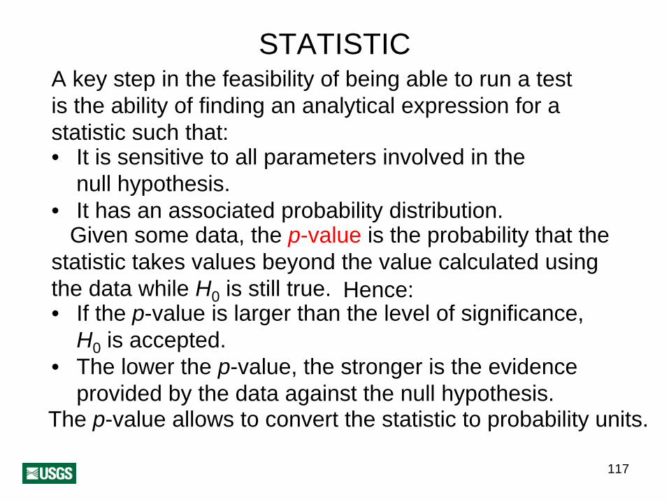
STATISTICA key step in the feasibility of being able to run a test is the ability of finding an analytical expression for a statistic such that:• It is sensitive to all parameters involved in the
null hypothesis.• It has an associated probability distribution.
Given some data, the p-value is the probability that the statistic takes values beyond the value calculated using the data while H0 is still true. • If the p-value is larger than the level of significance,
H0 is accepted.• The lower the p-value, the stronger is the evidence
provided by the data against the null hypothesis.The p-value allows to convert the statistic to probability units.
Hence:

118
SAMPLING DISTRIBUTION
The sampling distribution of a statistic is the distribution of values taken by the statistic for all possible random samples of the same size from the same population. Examples of such sampling distributions are:• Standard normal and the t-distributions for the
comparison of two means.• The F-distribution for the comparison of two
variances.• χ 2The distribution for the comparison of two
distributions.

119
PROBABILITY REMINDER AND P-VALUES
[ ] ( )dxxfxXx
∫=≤1
1Prob [ ] ( )dxxfxXx∫∞
=> 1Prob∞−
Example:
[ ] (
90.0
1,0;Normal28.1Prob28.1
=
=≤ ∫∞−
dxxX
[ ] (
10.0
1,0;Normal28.1Prob28.1
=
=> ∫∞
dxxX
)
)
1
In this example, assuming a one-sided test, when the statistic is 1.28, the p-value is 0.1 (10%).
120
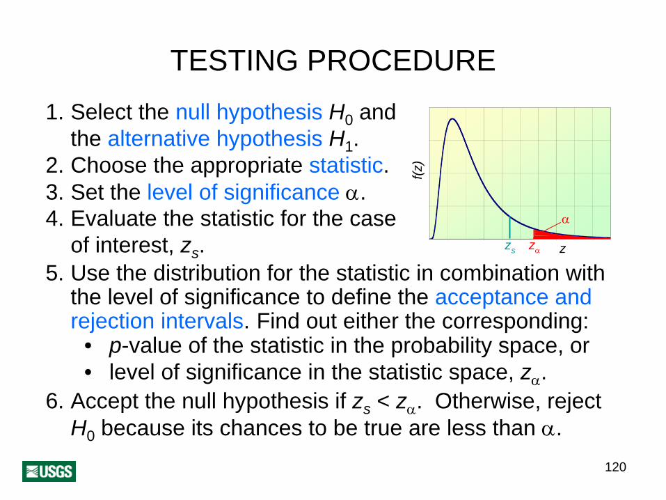
TESTING PROCEDURE
5. Use the distribution for the statistic in combination with the level of significance to define the acceptance and rejection intervals. Find out either the corresponding:
• p-value of the statistic in the probability space, or• level of significance in the statistic space, zα.
6. Accept the null hypothesis if zs < zα. Otherwise, rej ect
H0 because its chances to be true are less than α.
1. Select the null hypothesis H0 and the alternative hypothesis H1 .
2. Choose the appropriate statistic.3. Set the level of significance α. 4. Evaluate the statistic for the case
of interest, zs .α
zαzs z
f(z)

121
PARAMETER TESTING

122
TESTING TWO MEANS
123
INDEPENDENCE
The random outcomes A and B are statistically independent if knowing the result of one does not change the probability for the unknown outcome of the other.
Prob[A | B] =Prob[A]For example:• Head and tail in successive flips of a fair coin are independent events.• Being dealt a king from a deck of cards and having two kings on the table are dependent events.

124
TESTING PARENT POPULATIONS
Given a sample, the interest is on whether the values are a partial realization of a population with known mean and variance.
A one-sided test would be:
H0 : mn ≤ μp
H1 : mn > μp
wheremn is the sample mean,μp is the population mean,σ 2
p is the population variance.
125
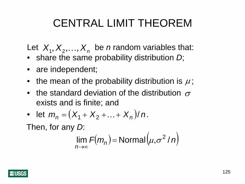
CENTRAL LIMIT THEOREM
X1, X2,K, XnLet be n random variables that:• share the same probability distribution D;• are independent;• μthe mean of the probability distribution is ;• σthe standard deviation of the distribution
exists and is finite; and• l mn = X1 + Xet +K2 + Xn / n .( )Then, for any D:
lim F(m ) =Normal ( ,μ σ 2n /n)
n→∞
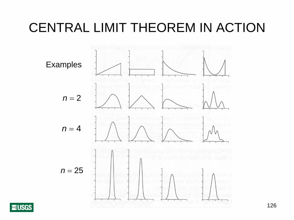
CENTRAL LIMIT THEOREM IN ACTION
126
2=n
4=n
25=n
Examples

127
STANDARD NORMAL DISTRIBUTIONAs mentioned before, standardization is the transformation obtained by subtracting the mean from each observation and dividing the result by the standard deviation.
In the Central Limit case:
( )1,0Normal
0
0.1
0.2
0.3
0.4
0.5
-4 -3 -2 -1 0 1 2 3 4
z
f(z)
nm
zp
pn
/1σμ−
=
Thus, in this case, the appropriate statistic is the sample mean standardized by employing the population parameters. By the Central Limit theorem, this statistic follows a standard normal distribution, N(0,1).

128
EXAMPLE Size Mean Stand. dev.
Population 16.5 6.0 Sample 25 18.0
1. H0 : mn ≤ μp
H1 : mn > μp
2. α = 0.05 5%( )3. The statistic is z-score.
18 −16.54. zs = =1.25
6 1/ 255. For a Normal(0,1)
distribution, the
cumulative probability is 0.05 above zα = 1.65.6. zs <zα H0, therefore, is accepted.
0
0.1
0.2
0.3
0.4
0.5
-4 -3 -2 -1 0 1 2 3 4
z
f(z)
1.651.25

129
INFLUENCE OF SAMPLE SIZEThe table shows sensitivity of the results to sample size when the experimental mean remains fixed at 18.0 in the previous example.
The larger the sample size, the more likely a rejection.• Specification of sample size adds context to a test.• Specificity of a test is poor for small sample sizes.• For large sample sizes, findings can be statistically
significant without being important.
Sample size
Statistic zs
P-value, percent
Ho(α=5%)
10 0.79 21.48 Accepted25 1.25 10.16 Accepted
100 2.50 0.62 Rejected 250 3.95 0.01 Rejected

130
DEGREES OF FREEDOMIn the calculation of a statistic, the number of degrees of freedom is the number of values free to vary.
The number of degrees of freedom for any estimate is the number of observations minus all relationships previously established among the data. The number of degrees of freedom is at least equal to the number of other parameters necessary to compute for reaching to the calculation of the parameter of interest.
For example, for a sample of size n, the number of degrees of freedom for estimating the variance is n – 1 because of the need first to estimate the mean, after which one observation can be estimated from the others. For example:
( nn xxx
nxxxnx +++−
+++⋅= K
44 344 21
K32
211
mean
)

131
STUDENT’S T-DISTRIBUTION
We have seen that the mean of any independent and identically distributed random variables is normal provided that:• One knows the means and variance of the
population.• The sample size is large. The rule of thumb is that
a size above 30 is large.The Student’s t distribution operates analogously to
N 0,1( )the standard normal distribution, , and should be used instead when any of the requirements above is not met.

132
EXAMPLES OF T-DISTRIBUTIONS
Probability density function Cumulative distribution function
k is the degrees of freedom.

133
TESTING TWO VARIANCES
134
F-DISTRIBUTION
The F-distribution is another distribution particularly developed for statistical testing.
Its parameters are two degrees of freedom that vary independently from each other.
It is employed to test variances and it operates completely analogously to the other distributions: it provides a reference value based on which the null hypothesis is accepted or rejected according to a level of significance.
The main limitation is that the samples must come from normal distributions.
135
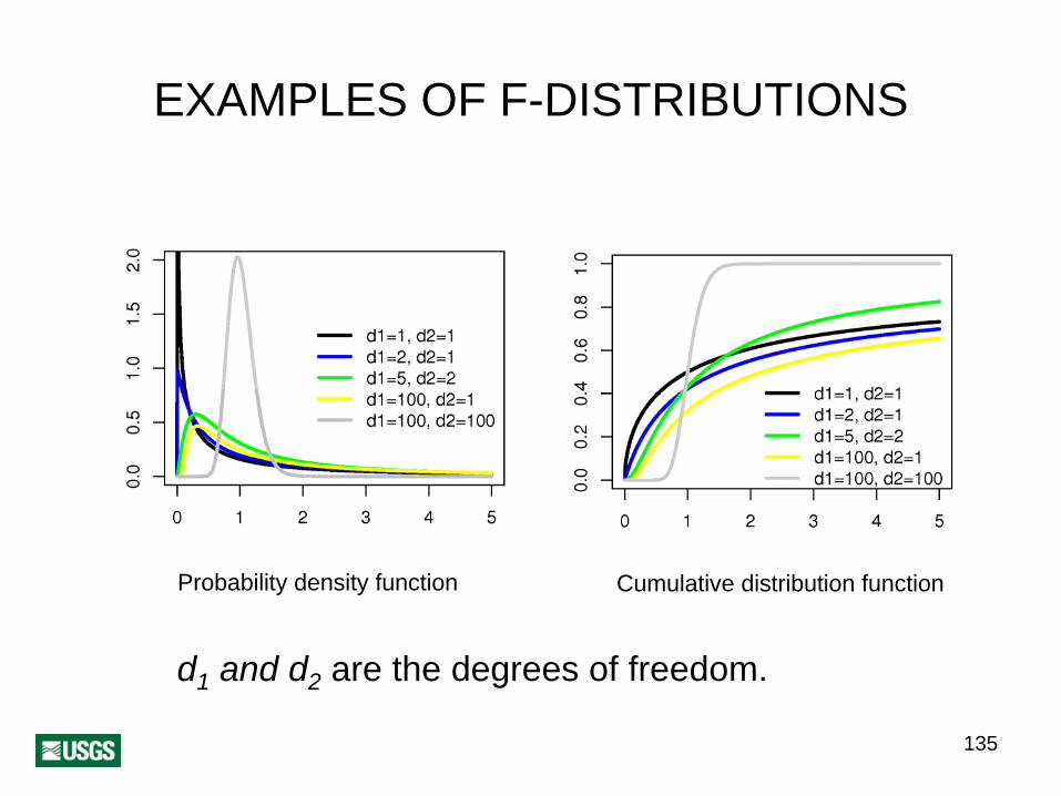
EXAMPLES OF F-DISTRIBUTIONS
Probability density function Cumulative distribution function
d1 and d2 are the degrees of freedom.
136
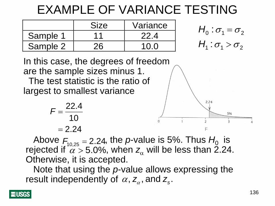
EXAMPLE OF VARIANCE TESTING Size Variance
Sample 1 11 22.4 Sample 2 26 10.0
211
210
::
σσσσ
>
=
HH
F
In this case, the degrees of freedom are the sample sizes minus 1.The test statistic is the ratio of
largest to smallest variance
24.210
4.22
=
=F
Abov F10,25 = 2.24e , the p-value is 5%. Thus H0 is rej α > 5.0%ected if , when zα will be less than 2.24. Otherwise, it is accepted.
Note that using the p -value allows expressing the result independently of ,α zα , and zs.

137
TESTING MORE THAN TWO MEANS

138
ANALYSIS OF VARIANCE• Analysis of variance is an application of the F-test for the
purpose of testing the equality of several means.• Strategies and types of variances abound, but it all
revolves around calculating some variances and then proving or disproving their equality.
• The interest is on deciding whether the discrepancies in measurements are just noise or part of a significant variation.
• The simplest form is the one-way ANOVA, in which the same attribute is measured repeatedly for more than two specimens:
H0 : μ1 = μ2L = μk ,k ≥ 3H1 : at least one mean is different.
• In this case, the variances going into the statistic are the variance for the mean among localities and the variance within specimens.

139
ONE-WAY ANOVA TABLE
Source of Degrees of variation Sum of squares freedom Variance F test statistic
Among localities SSA m - 1 MSA MSA / MS EWithin specimens
(“Error”) SSE N - m MSE
Total Variation SST N - 1
number of localitiesnumber of specimensspecimen i for locality j
∑ ∑= =
⎟⎟⎠
⎞⎜⎜⎝
⎛−=
m
j
n
ijijE XxSS
1
2
1
:n:m
∑=
=n
iijj x
nX
1
1
mnN ⋅=
∑∑= =
=m
j
n
iijx
NX
1 1
1
2
1∑=
⎟⎠⎞⎜
⎝⎛ −=
m
jjA XXSS
:ijx
∑∑= =
⎟⎠⎞⎜
⎝⎛ −=
m
j
n
iijT XxSS
1 1
2mN
SSMS EE −=
1−=
mSSMS A
A

140
EXAMPLEShell width, mm
Specimen Locality 1 Locality 2 Locality 3 Locality 4 Locality 5 1 16.5 14.3 8.7 15.9 17.62 17.3 16.1 9.5 17.6 18.43 18.7 17.6 11.4 18.4 19.14 19.2 18.7 12.5 19.0 19.95 21.3 19.3 14.3 20.3 20.26 22.4 20.2 16.5 22.5 24.3
510152025
0.5 1 1.5 2 2.5 3 3.5 4 4.5 5 5.5Replicates
Car
bona
te, %
+ + +
+
+
Specimens
Wid
th, m
m
Source of Degrees of variation Sum of squares freedom Variances F test statistic
Among localities 237.42 4 59.35 10.14 Within specimens
(“Error”) 146.37 25 5.85
Total Variation 383.79 29
F4,25 = 10.When 14, p = 0. 00005 α > 0 , so for .00005, at least one mean is significantly different from the others.

141
DISTRIBUTIONAL TESTING

142
χ 2THE DISTRIBUTION
X1, X2,K, XkLet be k random variables that:• are independent;• are all normally distributed;• μ ithe means are not necessarily equal;• σ ieach distribution has a standard deviation ,then, the sum of the standardized squares
∑∑==
⎟⎟⎠
⎞⎜⎜⎝
⎛ −=
k
i i
iik
ii
xz1
2
1
2
σμ
χ 2kfollows a distribution with k degrees of
freedom. Like the t-distribution, lim 2kχ =N(0,1) .
k→∞

143
χ 2EXAMPLES OF DISTRIBUTIONS
Probability density function Cumulative distribution function
k is the degrees of freedom.

144
n.
χ 2TEST OF FITNESS
χ 2k can be used to test whether the relative frequencies of
an observed event follow a specified frequency distribution. The test statistic is
( )∑=
−=
n
i
ii
EEO
1
22
i
χ
Oi is an observed frequency for a given class,Ei is the frequency corresponding to the target distributio
χ 2kAs usual, if the statistic lands beyond the value of
corresponding to the degrees of freedom k and level of αsignificance , the null hypothesis is rejected.
Weaknesses of the test are:• result depends on the number of classes, • no class can be empty,• there must be at least 5 observations per class for at
least 80% of the classes.
145
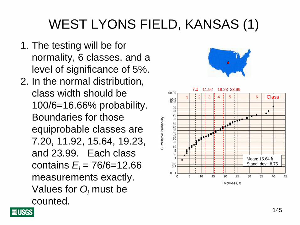
WEST LYONS FIELD, KANSAS (1)1. The testing will be for
normality, 6 classes, and a level of significance of 5%.
2. In the normal distribution, class width should be 100/6=16.66% probability. Boundaries for those equiprobable classes are 7.20, 11.92, 15.64, 19.23, and 23.99. Each class contains Ei = 76/6=12.66 measurements exactly. Values for Oi must be counted.
Mean: 15.64 ftStand. dev.: 8.75
1 2 3 4 6
7.2 11.92
5
23.9919.23
Class

146
WEST LYONS FIELD, KANSAS (2)4. In this case, the statistic is:
)
( )
( ) ( ) 94.266.12
66.121166.12
66.121566.12
66.121066.12
66.121266.12
66.121766.12
66.1211
22
22222
=−
+−
+
−+
−+
−+
−=sχ
( ) ( ) ( )
f(x)
x2.94 9.49
( )42χ5. We have calculated two
parameters (mean and standard deviation). So the there are 6 - 2 = 4 degrees of freedom.
6. χ 2αFor a level of significance of 5%, 4,0.05 = 9.49 .
χ 2 < χ 2s αSo, because , there is no evidence to suggest
that the thickness values are not normally distributed.
(

147
KOLMOGOROV-SMIRNOV TEST
This is a much simpler test than the chi-square test because:• The result does not
depend on the number of classes.
• It is nonparametric.The statistic is the
maximum discrepancy, D, between the two
.)Fn (xcumulative distributions F x and under comparison
D = max(Fn (x −F x )) ( )( )
148
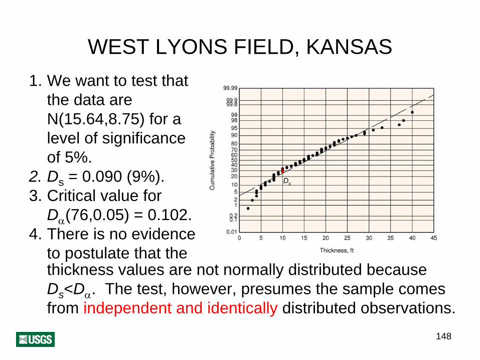
WEST LYONS FIELD, KANSAS1. We want to test that
the data are N(15.64,8.75) for a level of significance of 5%.
2. Ds = 0.090 (9%).3. Critical value for
Dα
(76,0.05) = 0.102.4. There is no evidence
to postulate that thethickness values are not normally distributed because Ds <Dα
. The test, however, presumes the sample comes from independent and identically distributed observations.
Ds

149
Q-Q AND P-P PLOTSScatterplots of the quantiles andthe cumulative probabilities of the two distributions are the ultimate tests in terms of simplicity.• If the distributions are the same, the
points align along the main diagonal.• There is no statistic or level of
significance for evaluating the results.
• P-P plots are insensitive to shifting and scaling, and the vertical scale is in the same units as in Kolmogorov- Smirnov test.
• The Q-Q plot is good here at calling the user’s attention about the normal
West Lyons field
PP
distribution being able to take negative values.

150
FINAL REMARKS
151
SPATIOTEMPORAL DEPENDENCEMany natural phenomena exhibit fluctuations that show continuity in space and time. Continuity denotes the common experience that in proximity of any observation, another measurement will be approximately the same.• Given a spatiotemporally continuous phenomenon
and the location of an observation, close proximity does tell something about the outcome of a second observation; they are not necessarily independent.
• The degree and extent of this dependence can be estimated through the semivariogram.
• Modeling spatiotemporally dependent data, often in the form of maps, is the realm of geostatistics.

152
SEMIVARIOGRAM
1000 random numbers
Spatial independence
Gravimetric anomaly, Elk Co., KS
Spatial dependence

153
7. MULTIVARIATE STATISTICS

154
METHODSMultivariate statistics deals with the analysis and display of objects with two or more attributes consistently measured for several specimens. The main motivations are better understanding of the data and interest in making simplifications.
The main families of methods available are:• cluster analysis• discriminant analysis• principal component analysis• factor analysis
While missing values are not an insurmountable problem, they are a situation to avoid. Often one missing value in a record requires dropping the entire record.
All methods are complex enough to require a computer for performing the calculations.

155
MATRICESA matrix is a rectangular array of numbers, such as A. When n = m, A is a square matrix of order n.
Matrices are a convenient notation heavily used in dealing with large systems of linear equations, which notablyreduce in size to just A X = B.
Transposing all rows and columns in A is denoted as AT.
[ ]'B mbbb L21=
[ ]'X mxxx L21=
⎥⎥⎥⎥
⎦
⎤
⎢⎢⎢⎢
⎣
⎡
=
nmnn
m
m
aaa
aaaaaa
L
LLLL
L
L
21
22221
11211
A
Main diagonal of a square matrix is the sequence of element a11 , a22 , …, ann from upper left to lower right.

156
CLUSTER ANALYSIS

157
AIMThe general idea is to group objects in attribute space into clusters as internally homogeneous as possible and as different form the other clusters as possible.
Different types of distances, proximity criteria, and approaches for preparing the clusters have resulted in several methods.
Some methods render results as dendrograms, which allow displaying the data in two dimensions.
Large distance increments provide the best criteria for deciding on the natural number of clusters.
0 2 4 6 8 10
Attribute 1
0
2
4
6
8
10
Attri
bute
2
1
2
3
45
6
A
B
C
A BC

158
DISSIMILARITIESIf Σ is the covariance matrix for a multivariate sample of m attributes, the following distances are the most common measurements for dissimilarity between vectors p and q:
• Euclidean, Manhattan,
Mahalanobis,
∑=
−i
ii qp1
( )∑=
−m
iii qp
1
2
( ) ( ).1
1∑=
− −−m
iqpΣqp '
•
•
m
Distances can be in original data space or standardized.Mahalanobis distances account for distance relative to
direction and global variability through the covariance matrix.Euclidean distances can be regarded as a special case of
Mahalanobis distance for a covariance matrix with ones along the main diagonal and zeros anywhere else.

159
PROXIMITY AND METHODS
Proximity between clusters is commonly decided based on the average inter-cluster distance. The most common methods are:
• Agglomerative hierarchical • Divisive hierarchical• K-means
Choice of dissimilarity measure may have greater influence in the results than the selection of the method.

160
DATA SET TO BE CLUSTEREDPhysical properties of carbonates
Mineral
Spec. gravity g/cc
Refractive index Smallest Largest
Hardness
Aragonite (ar) 2.94 1.530 1.685 3.7 Azurite (az) 3.77 1.730 1.838 3.7 Calcite (ca) 2.72 1.486 1.658 3.0 Cerusite (ce) 6.57 1.803 2.076 3.0 Dolomite (do) 2.86 1.500 1.679 3.7 Magnesite (mg) 2.98 1.508 1.700 4.0 Rhodochrosite (rh) 3.70 1.597 1.816 3.7 Smithsonite (sm) 4.43 1.625 1.850 4.2 Siderite (si) 3.96 1.635 1.875 4.3 Strontianite (st) 3.72 1.518 1.667 3.5 Witherite (wi) 4.30 1.529 1.677 3.3
Often all attributes are standardized to avoid the dominance of results by those with the largest numerical values.
161
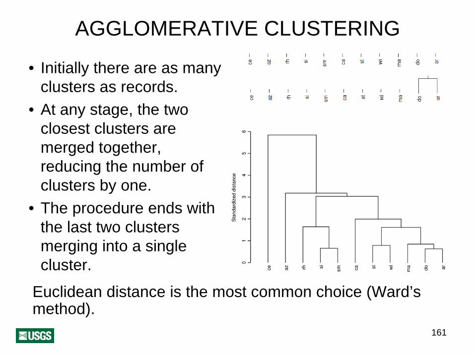
AGGLOMERATIVE CLUSTERING
• Initially there are as many clusters as records.
• At any stage, the two closest clusters are merged together, reducing the number of clusters by one.
• The procedure ends with the last two clusters merging into a single cluster.
Euclidean distance is the most common choice (Ward’s method).

162
DIVISIVE CLUSTERING
1. Initially all records are in one cluster.
2. At any stage, all distances inside each cluster are calculated.
3. The cluster with the largest specimen-to- specimen distance is broken apart, increasing the number of clusters by one.
163
DIVISIVE CLUSTERING
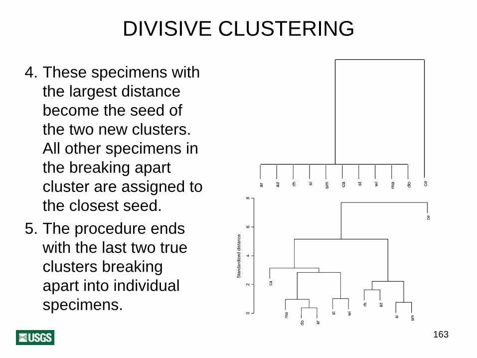
4. These specimens with the largest distance become the seed of the two new clusters. All other specimens in the breaking apart cluster are assigned to the closest seed.
5. The procedure ends with the last two true clusters breaking apart into individual specimens.

164
K-MEANS CLUSTERINGThe final number, k, of clusters is here decided at the outset. The algorithm is:1. Select the location of k
centroids at random. 2. All objects are assigned
to the closest centroid.3. Recalculate the location
of the k centroids.4. Repeat steps 2 and 3 until reaching convergence.The method is fast, but the solution may be sensitive to the selection of the starting centroids.
ca ce
doar
ma
rh
st
wi
azsmsi
k = 5

165
CLUSTERING REMARKS• The method is primarily a classification tool devoid of
a statistical background.• The more complex the dataset, the more likely that
different methods will generate different results.• The k-means methods is an extreme case, as even
different runs for the same number of clusters may produce different results.
• Often solutions are suboptimal, failing to perfectly honor the intended objective of the method.
• In the absence of clear cut selection criteria, convenience in the eye of the user remains as the ultimate consideration on choosing the number of final clusters and clustering method.
• If totally lost, go for the Ward’s method followed by the k-means method starting from the cluster generated by Ward’s method.

166
DISCRIMINANT ANALYSIS
167
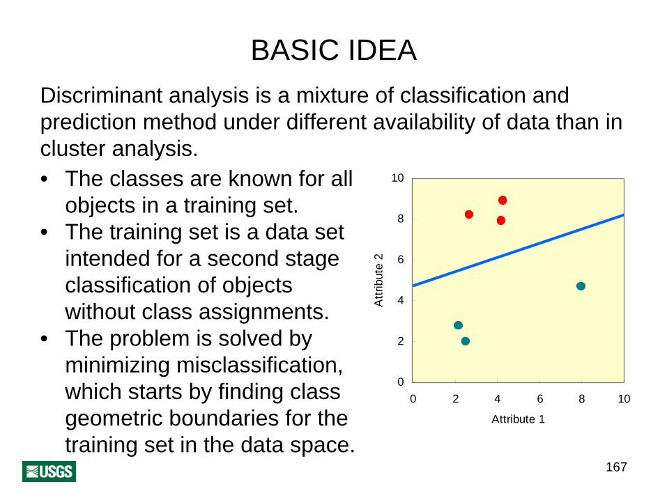
BASIC IDEADiscriminant analysis is a mixture of classification and prediction method under different availability of data than in cluster analysis.• The classes are known for all
objects in a training set.• The training set is a data set
intended for a second stage classification of objects without class assignments.
• The problem is solved by minimizing misclassification, which starts by finding class geometric boundaries for the training set in the data space.
0
2
4
6
8
10
0 2 4 6 8 10
Attribute 1
Attr
ibut
e 2

168
ASSUMPTIONS
• The data are a sample from a multivariate normal distribution. Thus, all attributes are normally distributed within each class.
• Any specimen has the same probability of belonging to any of the classes.
• None of the attributes is a linear combination of the others.
• The means for attributes across groups are not correlated with the variances.
Discriminant analysis is a true statistical method based on multivariate distribution modeling. Important assumptions for making the analysis possible are:
Although in practice all assumptions are never simultaneously satisfied, the formulations are robust enough to tolerate departures.

169
VARIANTSThere are different approaches to discriminant analysis, but the main difference is in the type of surfaces employed to establishing the class boundaries.• Linear methods, in which the surfaces are
hyperplanes in an m dimensional space, where m is the number of attributes considered in the analysis. Linear discriminant analysis results from assuming all classes have the same covariance matrix.
• Quadratic methods, in which the boundaries are polynomials of order up to 2, with each class having a different covariance matrix.

170
TESTS
The following tests are integral parts of the procedure:• Homogeneity of covariances• Equality of means• Normality
171
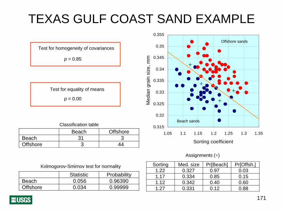
TEXAS GULF COAST SAND EXAMPLE
Test for homogeneity of covariances
p = 0.85
Test for equality of means
p = 0.00
0.315
0.32
0.325
0.33
0.335
0.34
0.345
0.35
0.355
1.05 1.1 1.15 1.2 1.25 1.3 1.35
Sorting coefficientM
edia
n gr
ain
size
, mm
Offshore sands
Beach sands
++
+
+
Classification table Beach Offshore
Beach 31 3Offshore 3 44
Kolmogorov-Smirnov test for normality
Statistic ProbabilityBeach 0.056 0.96390Offshore 0.034 0.99999
Assignments (+)
Sorting Med. size Pr[Beach] Pr[Offsh.] 1.22 0.327 0.97 0.03 1.17 0.334 0.85 0.15 1.12 0.342 0.40 0.60 1.27 0.331 0.12 0.88

172
PRINCIPAL COMPONENT ANALYSIS
173
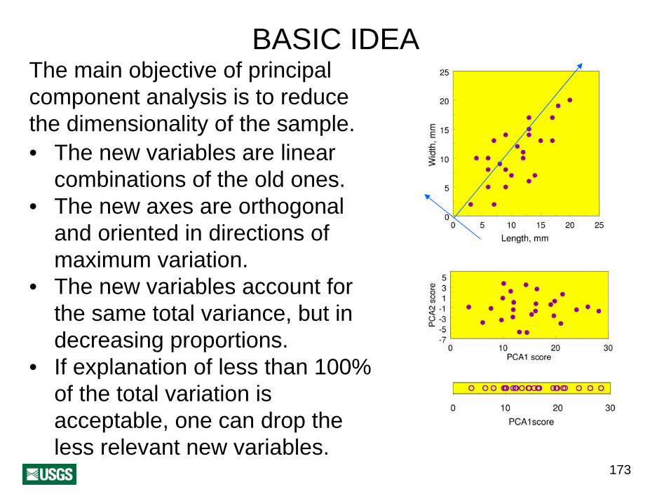
BASIC IDEAThe main objective of principal component analysis is to reduce the dimensionality of the sample. • The new variables are linear
combinations of the old ones.• The new axes are orthogonal
and oriented in directions of maximum variation.
• The new variables account for the same total variance, but in decreasing proportions.
• If explanation of less than 100% of the total variation is acceptable, one can drop the less relevant new variables.

174
MATRIX TERMINOLOGYThe determinant of a square matrix, |A|, of order m is an expression having additive and subtractive products of m coefficients. The exact rules are complicated, but for order
= a ⋅a − a ⋅a .2, for example, 21122211AGiven a symmetric square
matrix, its eigenvalues are the solution, Λ, to the equation that results from subtracting the unknown value λ from the main diagonal of its determinant.
An eigenvector Xi is the solution to equation system obtained by subtracting an eigenvalue from all diagonalterms of A when B = 0.
0
21
22221
11211
=
−
−−
λ
λλ
mmmm
m
m
aaa
aaaaaa
L
LLLL
L
L
[ ]Tmλλλ L21=Λ
⎥⎥⎥⎥
⎦
⎤
⎢⎢⎢⎢
⎣
⎡
=
⎥⎥⎥⎥⎥
⎦
⎤
⎢⎢⎢⎢⎢
⎣
⎡
⎥⎥⎥⎥
⎦
⎤
⎢⎢⎢⎢
⎣
⎡
−
−−
0
00
2
1
21
22221
11211
MM
L
LLLL
L
L
mi
i
i
immmm
mi
mi
x
xx
aaa
aaaaaa
λ
λλ
175
METHODSolution to the problem comes from finding the orthogonal combination of attributes with maximum variance.
Given n records containing measurements for m attributes, one can calculate an m by m symmetric covariance matrix. The actual multivariate distribution is irrelevant.
The directions of maximum variance are provided by the eigenvectors in the form of directional cosines. The axes in the new system of reference remain orthogonal.
The length of each axis is taken as twice the eigenvalue.
Borrowing from the properties of matrices, the new axes are oriented along the directions of maximum variance and ranked by decreasing length.

176
BOX EXAMPLE
Variables
x1 = long edgex2 = middle edgex3 = short edgex4 = longest diagonal
radius of smallest circumscribe spherex5 = radius of largest inscribe spherelong edge + intermediate edgex6 = short edgesurface areax7 = volume

177
PRINCIPAL COMPONENTS EXAMPLE
Coefficient matrix
5.400⎡ ⎤3.2600.779
A 6.3912.1553.0351.996−
⎢⎢⎢⎢⎢⎢⎢⎢⎢⎣
=
5.8461.4656.0831.3122.8772.370−
2.7742.204 9.1073.839 1.611 10.7145.167 2.783 14.7741.740 3.283 2.252−
−−−
20.7762.622 2.594
⎥⎥⎥⎥⎥⎥⎥⎥⎥⎦
Χ =−
⎡⎢⎢⎢⎢⎢⎢⎢⎢⎢⎣
0.1640.1420.1730.1700.5460.768
Eigenvectors
0.422 0.645 0.2250.447 0.713 0.3950.257 0.130 0.629 0.6070.650 0.146 0.2120.135 0.105 0.164 0.1610.133 0.149 0.2070.313 0.719 0.596
Orientation
−
−−
−−−
−
−
−−
−−−− −
−
0.415
0.2800.4030.5960.4650.107
−
−
0.3850.3290.2110.5650.5140.327
⎤⎥⎥⎥⎥⎥⎥⎥⎥⎥⎦
of second new axis
Eigenvalues
Λ = [34.491 18.999 2.539 0.806 0.341 0.033 0.003]T
0
20
40
60
80
100
120
1 2 3 4 5 6 7Principal components
Cum
ulat
ive
expl
aine
d va
rianc
e

178
FACTOR ANALYSIS

179
INTENDED PURPOSEFactor analysis was originally formulated in psychology to assess intangible attributes, like intelligence, in terms of abilities amenable of testing, such as reading comprehension.
Principal component analysis can be used to run a factor analysis, which sometimes contributes to confusion of the two methods.
Principal component factor analysis employs a correlation coefficient matrix obtained after standardizing the data.
180
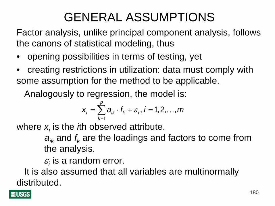
GENERAL ASSUMPTIONSFactor analysis, unlike principal component analysis, follows the canons of statistical modeling, thus• opening possibilities in terms of testing, yet• creating restrictions in utilization: data must comply with some assumption for the method to be applicable.
Analogously to regression, the model is:
distributed.
mifax i
p
kkiki ,,2,1,
1K=+⋅= ∑
=
ε
where xi is the ith observed attribute.aik and fk are the loadings and factors to come from the analysis.
i ε is a random error.It is also assumed that all variables are multinormally

181
VARIANTS
The two main approaches to factor analysis are:• principal components• maximum likelihood
In addition to the general assumptions, maximum likelihood factor analysis assumes that:• Factors follow a standard normal distribution, N(0, 1).• All of the factors are independent.• The correlation coefficient matrix prepared with the
data is a good approximation to the population correlation coefficient matrix .

182
BOX EXAMPLE REVISITED
Variables
x1 = long edgex2 = middle edgex3 = short edgex4 = longest diagonal
radius of smallest circumscribe spherex5 = radius of largest inscribe spherelong edge + intermediate edgex6 = short edgesurface areax7 = volume

183
PRINCIPAL COMPONENT FACTOR ANALYSIS FOR THE BOX EXAMPLE
Coefficient matrix
1.000⎡ ⎤0.5800.201
A 0.9110.2830.2870.533−
⎢⎢⎢⎢⎢⎢⎢⎢⎢⎣
=
1.0000.3640.8340.1660.2610.609−
1.0000.439 1.0000.704 0.163 1.0000.681 0.202 0.9900.649 0.676 0.427−
−−−
1.0000.357 1.000
⎥⎥⎥⎥⎥⎥⎥⎥⎥⎦
Χ =
−−−−
⎡⎢⎢⎢⎢⎢⎢⎢⎢⎢⎣
0.4050.4320.3850.4940.128
0.481
Eigenvectors (Factors)
0.293 0.667 0.2270.222 0.698 0.4370.356 0.148 0.628 0.5120.232 0.119 0.210 0.1050.575 0.111 0.3890.580 0.174 0.3550.130 0.735 0.455
Orientation
−−
−
−
−
−−
−−−
−
0.4100.1440.1880.5880.4230.500
−
−
0.2780.2540.1080.5360.5560.497
⎤⎥⎥⎥⎥⎥⎥⎥⎥⎥⎦
of secondnew axis
Eigenvalues
Λ = [3.395 2.805 0.437 0.278 0.081 0.003 0.000]T
0
10
20
30
40
50
60
70
1 2 3 4 5 6 7
New axes
Tota
l var
ianc
e, p
erce
nt
Principal component analysis
Factor analysis

184
ACKNOWLEDGMENTS

185
I am indebted for the valuable suggestions received as part of the review process of these notes from Emil Attanasi (U.S. Geological Survey), Geoffrey Bohling (Kansas Geological Survey), and Vera Pawlowsky-Glahn (Universitat de Girona, Spain). I am also grateful to early participants of my lectures who contributed with their remarks to make corrections and reformulate some topics. Eric Morrissey (U. S. Geological Survey) added tags to facilitate use of the notes by visually impaired readers.

186
BIBLIOGRAPHY

187
Aitchison, J., 2003, The statistical analysis of compositional data: Blackburn Press, Caldwell, NJ, reprint, 416 p.Ambler. S., 2003, Agile Database Techniques: Effective Strategies for the Agile Software Developer: John Wiley
& Sons, New York, 480 p.Buccianti, A., G. Mateu-Figueras and V. Pawlowsky-Glahn, editors, 2006, Compositional data analysis from
theory to practice: The Geological Society, London, Special Publication No. 264, 212 p. Chernick, M. R., 2008, Bootstrap Methods: A Guide for Practitioners and Researchers: Wiley Interscience,
Hoboken, NJ, second edition, 369 p.Davis, J. C., 2002, Statistics and Data Analysis in Geology: John Wiley and Sons, New York, third edition, 638 p.Donnelly, R. A., Jr., 2007, The Complete Idiot’s Guide to Statistics: Alpha, New York, second edition, 395 p.Good, P. I. and J. W. Hardin, 2006, Common Errors in Statistics (and How to Avoid Them): Wiley Interscience,
Hoboken, NJ, 254 p.Hastie, T., R. Tibshirani, and J. Friedman, 2001, The Elements of Statistical Learning—Data Mining, Inference,
and Prediction: Springer, New York, 533 p.Helsel, D. R., 2004, Nondetects and Data Analysis: Wiley Interscience, Hoboken, NJ, 268 p.Holmgren, E. B., 1995, The P-P Plot as a Method for Comparing Treatment Effects: Journal of the American
Statistical Association, vol. 90, no. 429, p. 360-365.Jackson, S. L., 2005, Statistics Plain and Simple: Thomson Wadsworth, Belmont, CA, 269 p.Moore, D. S. and W. I. Notz, 2006, Statistics—Concepts and Controversies: Freeman, New York, sixth edition,
561 p.Salkind, N. J., 2007, Statistics for People Who (Think They) Hate Statistics: Sage Publications, Thousand Oaks,
CA, 402 p.Thomsen, V., D. Schatzlein, and D. Mercuro, 2003, Limits of detection in spectroscopy:
www.spectroscopyonline.com, vol. 18, no. 12, p. 112-114,Venables, W. N. and B. D. Ripley, 2003, Modern Applied Statistics with S: Springer, New York, 495 p.Walpole, R. E., R. H. Myers, S. L. Myers, and K. Ye, 2006, Probability and Statistics for Engineers and
Scientists: Prentice Hall, eighth edition, 848 p.

188
INDEX

189
accuracy 13, 15 agglomerative hierarchical method
159, 161 alternative hypothesis 112–113,
115, 120 analysis
cluster 156–165, 167 descriptive 38 discriminant analysis 167-171 factor 179–183 principal component 173–177,
179–181, 183 variance 138-140
arithmetic mean 47 assignment 167, 171 autocovariance 97 Bayes’s theorem 66 bias 95 binomial distribution 68 bootstrap method 76, 109–110 box-and-whisker plot 59 causality 88 central limit theorem 125–127 Chebyshev’s theorem 53 chi-square
distribution 142–143 test 144–147
classification 167, 169 cluster analysis 156–165, 167 coefficient
kurtosis 63
quartile skew 62 skewness 61, 69
coin flipping 68, 71, 75, 123 compositional data 98–99 conditional probability 66 correlation 98
coefficient 82, 86, 88, 179 covariance 81–82, 97, 158,
169–171 matrix 158, 169, 175
cumulative distribution 43 decile 56 degrees of freedom 130, 132,
134–135, 142–144, 146 dendrogram 157 dependent variable 84 detection limit 21–27, 101–110
instrumental 24 method 25 quantitation 26
determinant 174 discriminant analysis 167–171 dissimilarity 96, 159 distance 157–158
Euclidean 158, 161 Mahalanobis 158 Manhattan 158
distribution 67, 125 binomial 68 chi-square 142–143 continuous 67
discrete 67 F 134–135 Gaussian 43, 63, 69–70,
104–105, 125–128, 131, 134, 142, 145, 148, 168, 170, 180
lognormal 69, 105 normal 43, 63, 69–70,
104–105, 125–128, 131,134, 142, 145, 148, 168, 170, 180
sampling 119 student’s t 131–132 testing 142–149
divisive hierarchical method 159, 162–163
eigenvalue 174–175, 177, 183 eigenvector 174–175, 177, 183 error 85
mean square 86–87 propagation 94 Type I 114 Type II 114
Euclidean distance 158, 161 expected value 71–73, 81 explanatory variable 84–85 extreme value 54, 59 factor 180–181
analysis 179–183 F-distribution 134–136, 140 fractile 56 frequency table 40–41

190
Gaussian distribution 43, 63, 69–70, 104–105, 125–128, 131, 134, 142, 145, 148, 168, 170, 180
geometric mean 47, 110 geostatistics 151 histogram 42, 67, 75 hypothesis 120
alternative 112–113, 115, 120 null 112–117, 120, 128–129,
134, 144 independence 123, 148, 151, 152,
181 independent variable 84, 142 instrumental detection limit 24 interquartile range 57–58 k-means method 159, 164–165 Kaplan-Meier method 107, 110 Kolmogorov-Smirnov test 147–149,
171 kurtosis 63 legacy data 29–34 level of significance 114, 116–117,
120, 134, 144, 146, 149 limit of quantitation 26 linear
correlation 82 method 169 regression 86–87
lognormal distribution 69, 105 log-ratio transformation 99, 109
lurking variable 88 Mahalanobis distance 158 main diagonal 155, 174 Manhattan distance 158 matrix 155, 174–175, 177, 183
correlation coefficient 179, 181 covariance 158, 169, 175 order 155, 174 square 155
maximum 54 likelihood method 104–105,
110, 181 mean 47, 50, 59, 69, 72, 81, 91,
105, 124–125, 131, 142, 146, 168, 170–171
arithmetic mean 47 geometric mean 47, 110 testing 124–128, 138–140
measure centrality 46–49 dispersion 51–58 shape 60–63
median 48, 50, 56 method
agglomerative hierarchical 159, 161
bootstrap 76, 109–110 detection limit 25 divisive hierarchical 159,
162–163 k-means 159, 164–165
linear 169 Kaplan-Meier 107, 110 maximum likelihood 104–105,
110, 181 Monte Carlo 75–76 quadratic 169 replacement 103, 110 Ward’s 161, 165
minimum 54 mode 49 moment 73 Monte Carlo method 75–76, 94,
109 noise 87, 152 nonlinear regression 87 normal distribution 43, 63, 69–70,
104–105, 125–128, 131, 134, 142, 145, 148, 168, 170, 180
null hypothesis 112–117, 120, 128–129, 134, 144
outlier 58 order 155, 174 P-P plot 92, 149 p-value 117, 119–120, 136 percentile 56 plot
P-P 92, 149 Q-Q 90, 149
population 36, 124 power 114 precision 14–15, 101
191
principal component analysis 173–177, 179–181, 183
probability 65, 70, 117–118 conditional 66 density function 67
probability-probability plot 92, 149 proximity 159 Q-Q plot 90, 149 quadratic method 169 quantile 56 quantile-quantile plot 90, 149 quartile 56–57, 59, 105 radius of influence 97 random variable 37, 75 range 97 regressed variable 84 regression 84–88, 180 regressor 84 replacement method 103, 110 response variable 84 robustness 50, 87, 168 sample 36, 95
size 38, 105, 129–131 sampling distribution 118 scatterplot 80, 149 semivariogram 96–97, 151–152 significant digit 17–19 sill 97 simulation 75 skewness 61, 69
standard deviation 53, 69, 91, 125, 142, 146
standardization 91–92, 127, 142, 158, 160, 179
statistic 45, 76, 109, 116–120, 144, 146, 147, 149
statistics 4–8, 37, 127, 136 student’s t distribution 131–132 test
chi-square 144–146 distribution 142–149 Kolmogorov-Smirnov 147–148,
171 one-sided 113, 116, 123 two-sided 113, 116, 140 mean 124–128, 138–140 variance 134–136
theorem Bayes’s 66 central limit 125–127 Chebyshev’s theorem 53
unbiasedness 95–96 uncertainty 5, 94 variable
dependent 84 explanatory 84–85 independent 84 lurking 88 random 37, 75 regressed 84 response 84
variance 52–53, 73, 97, 105, 124, 134, 136, 138, 168, 173, 175
variate 37, 75 testing 134–136
Ward’s method 161, 165