basic research concepts distribute

16

CHAPTER 2

2.1 INTRODUCTION

Basic understanding of research methods is needed to understand and interpret statistical results. This chapter is a brief, nontechnical introduction to selected research methods terms mentioned in the GAISE (GAISE College Report ASA Revision Committee, 2016) numeracy guidelines in Chapter 1.

The design of an investigation refers primarily to the distinction between designs in which investigators have a high degree of control over the research situation (such as experiments) and situations in which researchers have little or no control (nonexperimental studies). Experimental methods of control include techniques such as random assignment of participants to groups and holding variables other than the treatment variable constant. Statistical methods of control are included in some types of analysis. Other design issues are discussed in greater detail in research methods textbooks (e.g., Cozby & Bates, 2017).

Data (or data set) refers to information, usually in numerical form in a computer file, about multiple cases and/or multiple variables.

Analysis refers to statistical techniques.A variable is a characteristic that differs or varies across subjects or cases. Examples of

variables for human research participants include sex, height, heart rate, and salary.Subjects or cases are the entities or observational units studied. In psychological

research, cases are usually individual persons or nonhuman animals. In other disciplines, cases can be different kinds of entities; for example, in sociology, a case can be a group or an organization; in political science, a case may be a nation; in forestry, a case may be a geographic location.

The terms sample and population are often used differently in ideal textbook situations than in many real-life research situations, as discussed in Section 2.11. For now, it is sufficient to say that a sample is a subset of a population; that is, a sample consists of cases selected from a population.

A generalization is a statement that results obtained for people and situations included in a study are applicable to other people and situations not included in the study. Ability to generalize results from a sample to a population depends on similarity of the sample to the population of interest.

Examples of errors in interpretation include (a) generalizing results more widely than can be justified, (b) arguing that one variable causes another variable when there is not enough evidence to support that claim, and (c) misunderstanding the limits of research methods and statistical analyses. Other types of error are possible.

BASIC RESEARCH CONCEPTS

Copyright ©2021 by SAGE Publications, Inc. This work may not be reproduced or distributed in any form or by any means without express written permission of the publisher.

Do not

copy

, pos

t, or d

istrib

ute

ChAPTER 2 • BASIC RESEARCh CONCEPTS 17

2.2 TYPES OF VARIABLES

2.2.1 Overview

It is useful to distinguish between categorical variables and quantitative variables (Jaccard & Becker, 2009). Scores for categorical variables tell us which group or category each case belongs to (e.g., whether a person is male or female). Scores for quantitative variables provide information about the amount of something (for example, height). Some psychologists make further distinctions among levels of measurement; see Appendix 2A for discussion. Two addi-tional types of variables are discussed in this section: rating scales and ordinal (also called rank).

2.2.2 Categorical Variables

Categorical variables identify group (or category) membership for each case. They are also called nominal variables because numbers serve only as names or labels for groups. This is a common type of variable. Examples of categorical variables include sex (for example, with group membership coded 1 = male, 2 = female) and marital status (with values coded 1 = never married, 2 = divorced, 3 = currently married). Additional categories could be included; for example, marital status could include categories such as engaged, cohabiting, separated, and remarried. Numerical values used for categorical variables are arbitrary; we could code divorced as 3 instead of 2, and this change in group numbering will make no difference in results of analyses.

When numbers are only labels for group membership, it is not meaningful to compare these numbers in terms of “greater than” or “less than.” A person whose marital status is rep-resented by the number 2 (divorced) is not greater than or better than a person whose marital status is represented by 1 (never married). We can say only that these individuals differ in marital status. It makes no sense to apply arithmetic operations (+, –, ×, ÷) to numbers when they are used only as labels for group membership. It makes no sense to calculate statistics such as sample means for scores on categorical variables; for example, it would be nonsense to compute a mean marital status.

Often the number of different score values for a categorical variable is small. However, it is possible for categorical variables to have many different score values. For example, a categorical variable to identify choice of future career could include dozens of different possible careers.

2.2.3 Quantitative Variables

Quantitative variables indicate “how much” of some characteristic or behavior each case or person has. For example, we can measure height or blood pressure for each person. When numerical scores for these variables are compared, it makes sense to describe them in terms of “more than” and “less than.” A person who is 70 inches tall is taller than a person who is 65 inches tall. It is reasonable to apply arithmetic operations to numerical values for quantitative variables; we can add, subtract, multiply, and divide scores. Thus, it is reason-able to compute a mean for variables such as height. Quantitative variables are common in behavioral and social science research.

2.2.4 Ordinal Variables

Sometimes researchers rank subjects instead of measuring amount. For example, we could tag the runners in a race as 1, 2, 3, . . . last (the order of crossing the finish line). Alter-natively, we could measure running time in seconds. Variables with scores that correspond


Do not

copy

, pos

t, or d

istrib

ute

18 APPLIED STATISTICS I

to ranks are called ordinal variables. Later you will see that there are specific analyses for scores that are collected in the form of ranks or are converted to ranks to get rid of problems such as outliers. Ranks are not widely used in data collection in behavioral and social sciences; measurements of quantity are generally preferred.

2.2.5 Variable Type and Choice of Analysis

Categorical and quantitative variables require different types of descriptive statistics (Chapter 4), graphs (Chapter 5), and other statistical analyses. It is necessary to distinguish between categorical and quantitative variables to choose appropriate statistical techniques. For some variables the decision is easy. Clearly, height and age are quantitative; sex and mari-tal status are categorical. However, there are examples of variables that can be handled as either categorical or quantitative, as noted in the next section.

2.2.6 Rating Scale Variables

A Likert scale is a common response format in survey and personality research. A typi-cal Likert scale question consists of a statement (worded so that it expresses a clearly positive or negative view about an issue) followed by a choice among degree of agreement ratings, as in the following example; each person chooses the number that best represents his or her degree of agreement. Originally Likert scales included five degrees of agreement, but multiple-point rating scales often have different numbers of responses (such as seven).

Example: “I believe the president is doing a great job.”

1 2 3 4 5

Strongly disagree Disagree Neutral or don’t know Agree Strongly agree

If five-point ratings are evaluated according to the formal levels of measurement stan-dards proposed by Stevens (1946, 1951; see Appendix 2A), they lie somewhere between the ordinal (rank) and interval levels of measurement. Rating scores provide at least rank-order information (e.g., 4 represents stronger agreement than 3). However, the differences between scores probably don’t represent equal intervals; for example, the difference in degree of agree-ment represented by 4 versus 5 may not be the same as the difference between 3 and 4. Five-point rating scale scores fall into a gray area: probably more informative than ranks, but probably less informative than measurements that assume equal intervals. That leads to disagreement as to whether it makes sense to compute means and other statistics for variables rated on five-point scales. Authorities cited in Appendix 2B argue that is acceptable to treat rating scale variables as quantitative variables in some circumstances.

In practice, ratings on five-point scales can often be treated as either categorical or quan-titative variables, whichever makes more sense in a specific research situation. Scores for the question above could be used to divide people into five groups that have different degrees of agreement (i.e., used as a categorical variable). It would also be reasonable to compute a mean for ratings.

2.2.7 Scores That Represent Counts

Consider this survey question: “How many children do you want to have in the future?” Possible responses include none, one, and so forth. This is a quantitative variable; three chil-dren are more than two children. Unlike many other quantitative variables, scores for this variable have a limited number of possible values; it is rare in the United States to encounter persons who want more than four children. In a small sample, a researcher might find that the


Do not

copy

, pos

t, or d

istrib

ute


only responses to this question are zero, one, and two. In some analyses it may be convenient and informative to treat these scores as labels for group membership (e.g., Group 1 does not want any children, Group 2 wants only one child, and Group 3 wants two children). However, it is also reasonable to compute the mean number of children. For variables that consist of counts (e.g., number of children) and variables that represent ratings on degree of agreement or behavior frequency (as in Section 2.2.3), it sometimes makes more sense to handle them as categorical, and it sometimes makes more sense to treat them as quantitative.

2.3 INDEPENDENT AND DEPENDENT VARIABLES

The first statistical techniques you will learn are ways to describe scores for just one variable.However, real-world research usually begins with questions about the way two or more

variables are related. It often makes sense to identify one of the variables as the independent or predictor variable (X) and the other as a dependent or an outcome variable (Y). The deci-sion about which variable to identify as independent depends on the nature of the research question about the variables.

2.4 TYPICAL RESEARCH QUESTIONS

This section describes three types of research questions about the relationship between two variables. When we distinguish between independent and dependent variables, the independent variable is often denoted X and the dependent variable Y.

2.4.1 Are X and Y Correlated?

A researcher can simply ask whether scores on two variables (X and Y) tend to co-occur or go together (without assuming any causal connection between them). There are alternative ways to word this question, such as:

� Are scores on X and Y correlated?

� Do scores for X and Y tend to co-occur?

� Are high scores on X associated with high scores on Y?

� Are X and Y associated?

I prefer this wording: Are scores on X and Y statistically related?For this research question, it is not necessary to identify one variable as independent

and the other variable as dependent. The term correlated can refer specifically to the results of a Pearson r correlation analysis. However, researchers sometimes use the word correlated in a much broader sense, to refer to any statistical relationship between variables, even when information about the relationship comes from some statistic other than a correlation coef-ficient (for example, from an independent-samples t test). We can evaluate whether X and Y are statistically related by doing whatever statistical analysis is appropriate for the types of variables (categorical vs. quantitative).

The bivariate statistics described in later chapters provide different ways to evaluate the extent to which scores on two variables are statistically related. The specific statistic that is most appropriate for a pair of X and Y variables depends on the types of variables (categorical or quantitative) and other issues; see Section 2.10. We can evaluate whether X and Y are statistically related on the basis of the outcome of any of these bivariate statistical analyses.


Do not

copy

, pos

t, or d

istrib

ute


2.4.2 Does X Predict Y?

In this question, X is identified by the researcher as the predictor or independent vari-able; Y is the outcome or dependent variable. To predict means to anticipate or guess some-thing that will happen in the future. A predictor should occur before the outcome (or at least not after the outcome). This is called temporal precedence. If X happens before Y, X has temporal precedence.

Consider these examples. Does height at age 10 years (X) predict height at age 21 years (Y)? Do high school grades (X) predict college grades (Y)? When temporal precedence is clear, it does not make sense to reverse these variables, that is, to ask whether height at age 21 predicts height at age 10 or whether college grades predict high school grades.

2.4.3 Does X Cause Y?

This question can be worded in several similar ways; we can replace the word cause with words such as change, determine, increase, decrease, or influence.

Here are examples of questions about cause:

� Does the death of a spouse (X) cause depression (Y)?

� Does study time (X) increase exam score (Y)?

� Does social stress (X) influence blood pressure (Y)?

� Does cigarette smoking (X) increase the risk for lung cancer (Y)? Is cigarette smoking a risk factor for lung cancer? (If a variable is called a risk factor, this usually implies that there may be other risk factors or causes.)

Note that the word order in questions can vary, for example, Is exam score (Y) increased by amount of study time (X)? In this question, study time is still the independent variable (presumed cause), and exam score is the dependent variable.

We need stronger evidence for claims that X causes or influences Y than for claims that X merely predicts Y or that X co-occurs with Y. Keep in mind that no matter what results we obtain in one study of X and Y, we should not view those results as a final answer to any of these questions.

2.5 CONDITIONS FOR CAUSAL INFERENCE

When researchers select variables to include in a study, the first consideration is:

1. There should be a plausible theory that explains why X and Y might be related (cf. Brannon, Feist, & Updegraff, 2017).

It does not make sense to choose an X variable and a Y variable at random. Variables are selected because past research or theories suggest that they may be related in meaningful ways.

Three additional conditions should be considered when interpreting research results as potential evidence for causation (Cozby & Bates, 2017).

2. We can say that X and Y are associated only if we find that X and Y are related when we do an appropriate statistical analysis. To evaluate whether X and Y are statistically related (or correlated), you will use the statistical analyses that you will learn in later chapters, such as the independent-samples t test and Pearson correlation.


Do not

copy

, pos

t, or d

istrib

ute


The next condition is required for questions about prediction and causation.

3. We can say that X predicts Y only if X happens earlier in time than Y (or at least not later than Y) and, in addition, X is statistically related to Y.

Questions about causal relationships (does X cause or influence Y) require all these preceding types of evidence as well as this fourth additional type of evidence:

4. We can infer that X causes Y only if no other variables are plausible rival explanations for changes in Y. In other words, X must be the only possible explanation for changes in Y. This condition can be very difficult to satisfy, because rival explanatory variables are common in many research situations.

Rival explanatory variables (also called confounds or confounded variables) arise in situations where many variables (other than X) might cause or influence Y. Suppose a researcher wants to know whether social stress (X) causes higher blood pressure (Y). Many other variables, in addition to social stress, can influence blood pressure, including but not limited to cardio-vascular fitness, body weight, use of caffeine, alcohol, and other drugs, smoking, and family history of high blood pressure. Smoking and use of alcohol might well be correlated with or confounded with anxiety. We can evaluate whether anxiety influences high blood pressure only if we control for other explanatory variables (or take them into account in statistical analysis).

In experiments, we take other rival explanatory variables into account by using experi-mental controls, such as holding the variables constant. For example, a study may include only people who do not use any drugs that may influence blood pressure. In nonexperimental studies, we use statistical control to try to rule out effects of rival explanatory variables. Techniques to do this are not covered in this volume; they involve more advanced forms of analysis. When a more sophisticated type of analysis is performed, the correct answer to the question “Does stress cause high blood pressure?” may be that stress is one among many variables that predict, and may possibly influence, blood pressure. Whether experimental or statistical control is used, readers need to know what variables have and have not been controlled in some way.

When scores for two potential causal or independent variables co-occur, we say that they are confounded. If people who experience a lot of social stress in their everyday lives tend to smoke a lot, then social stress and smoking are confounded, and it may be difficult to separate their effects. If people who report high levels of social stress have high blood pressure, the real reason for this (or at least a partial explanation for this) may be that people with high levels of stress also smoke or drink heavily.

The next section describes the extent to which various research designs (including nonexperimental, experimental, and quasi-experimental) can provide the evidence needed to satisfy Conditions 2, 3, and 4.

2.6 EXPERIMENTAL RESEARCH DESIGN

A typical experimental research design includes two or more groups of cases; each group is exposed to a different type of treatment or different amount of treatment (such as a drug). Experiments require comparisons. If a researcher wants to evaluate the effects of caffeine (X) on heart rate (Y), the researcher needs to examine situations in which people do, and do not, receive caffeine (or situations in which people receive varying amounts of caffeine). In many studies, a control group that receives no treatment is included.

Figure 2.1 is a schematic outline of a simple experiment. Read from left to right: the researcher has a group of available participants. Participants are divided into groups using a


Do not

copy

, pos

t, or d

istrib

ute


method that should ensure that similar people are included in Groups 1 and 2. Often random assignment to treatment groups is used to do this. In this example, Group 1 receives a bever-age that does not contain caffeine; Group 2 receives a beverage that does contain caffeine. The outcome variable, heart rate, is measured after participants drink the beverage. Statistical analysis compares mean heart rate to see if people who consumed caffeine (Group 2) have a higher average heart rate than people who did not consume caffeine (Group 1). (A placebo control group could be added.) The independent-samples t test is one example of a statistic that provides information about the differences for means of Y across groups.

In behavioral and social sciences, experimental design typically includes several kinds of experimental control. One form of experimental control is that a researcher controls assign-ment of participants to groups. In many experiments, cases are assigned to groups randomly. The intended purpose of random assignment is to avoid a confound of preexisting subject characteristics with type of treatment. (Note that random sampling of participants from a population is not the same as random assignment of those participants to treatment groups.)

Here is an example of a potential confound of participant characteristics with type of treatment. Suppose that a researcher arbitrarily assigns people to groups. Suppose that people in Group 1 (who do not consume caffeine) have low anxiety levels; people in Group 2 (who consume caffeine) have high anxiety levels. If average heart rate is higher in Group 2, it will not be clear whether this is due to caffeine or to preexisting anxiety (or both). There is a confound between the independent variable X (whether caffeine is present, no or yes) and a personal characteristic (preexisting anxiety). Preexisting anxiety is a plausible rival explanatory variable; we cannot conclude that caffeine caused a higher heart rate unless we can control for, rule out, or get rid of the differences in anxiety between groups.

A common way to try to prevent confound of treatment with participant characteristics is random assignment of participants to groups or conditions. Random assignment means that each subject or case has an equal chance of being placed in either group. An example of a method of random assignment is tossing a coin for each person and assigning the person to the no-caffeine group for heads and to the caffeine group for tails. This should result in a mixture of high and low anxiety scores within each of the two groups, with the same average

Figure 2.1 Schematic Outline of Simple Experimental Design

Group 1

Group formed by researcher, perhaps byrandom assignment of persons to groups

Two types of treatment administered by researcher in similarsituations: 1 = no caffeine, 2 = caffeine

Group 2

Totalsample

How was totalsample obtained?

Types of people ingroups should besimilar (equivalent)

Has researcher doneanything else different tothese two groups thatwould create a rivalexplanatory variable orconfound?

Measure thedependent variableafter treatment

Statistical analysis

Caffeine

Y1 =HR

Comparemean HRbetweengroups –

Which grouphas higher

HR?Y2 =HR

No caffeine(control

condition)

Note: HR = heart rate.


Do not

copy

, pos

t, or d

istrib

ute


anxiety score in Group 1 as in Group 2. This should also make the groups similar on other participant characteristics, such as age, past experience with caffeine, and body weight. When it works well, random assignment of participants to conditions prevents confounds of most participant characteristics with type of treatment.

The researcher has control over the type and amount of treatment. In this example, the researcher controls whether each participant receives caffeine and the amount of caffeine.

The researcher can control other variables and tries to keep them the same across par-ticipants both between groups and within groups. This is called standardization and experi-mental control over other situational factors or extraneous variables. Variables that are not included in the research question are extraneous (not of interest) in the present study. Many things other than the caffeine administered by the researcher could influence heart rate (for example, time of day, whether the research assistant is calm or upset, and whether partici-pants know that they are consuming caffeine). To achieve standardization, ideally, all partici-pants would be tested at the same time of day; the behavior of the research assistant would be made consistent, perhaps by training or even the use of a script; and neither participants nor research assistants would know which drinks contain caffeine.

Researchers need background knowledge about their variables to understand what kinds of confounds they need to anticipate and avoid. For example, if heart rate is the depen-dent variable, the researcher needs to know what other factors (apart from the manipulated variable, caffeine) might influence heart rate.

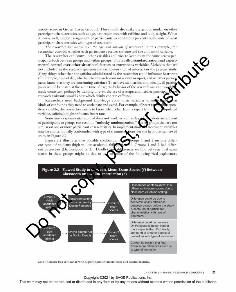
Sometimes experimental control does not work as well as hoped. Random assignment of participants to groups can result in “unlucky randomization,” that is, groups that are not similar on one or more participant characteristics. In implementation of a treatment, variables may be unintentionally confounded with type of treatment. Consider the hypothetical flawed study in Figure 2.2.

Figure 2.2 illustrates two possible confounds. First, Groups 1 and 2 include differ-ent types of students (high vs. low academic ability). Second, Groups 1 and 2 had differ-ent instructors (Dr. Feelgood vs. Dr. Deadly). Any differences we find between final exam scores in these groups might be due to one or more of the following rival explanatory

Figure 2.2 Flawed Study to Compare Mean Exam Scores (Y) Between Classroom and Online Instruction (X)

Note: There are two confounds with X: participant characteristics and teacher identity.

Group 1(high

academicability)

Group 2(low

academicability)

Group 1examscores

Group 2examscores

Researcher wants to know: Is adifference in exam scores due toclassroom vs. online setting?

Difference could be due toacademic ability differencebetween groups before the study.A confound of participantcharacteristics with type oftreatment.

Classroom settinginstruction run byDoctor Feelgood

Online course runby Doctor Deadly

Difference could be becauseDr. Feelgood is better liked ormore capable than Dr. Deadly; confound of another aspect ofprocedure with type of instruction.

Cannot be certain that finalexam score differences are dueto type of instruction.


Do not

copy

, pos

t, or d

istrib

ute


variables: classroom versus online setting, academic ability levels of students, and behaviors of the different instructors. We cannot conclude that classroom and online instruction cause different results on final exams unless we can rule out or get rid of the effects of the two confounded, rival explanatory variables (student ability and teacher identity). In many experi-mental situations, there are large numbers of potential confounds. See research methods text-books (such as Cozby & Bates, 2017) for further discussion of experimental control.

When potential confounds and extraneous variables can be ruled out by these forms of experimental control, an experiment can provide good-quality evidence that may be consis-tent with a researcher hypothesis about causal inference. (The results of a single study should not be considered proof of causal influence.) Nonexperimental designs lack all these types of experimental control. Quasi-experimental studies typically have some, but not all, of these forms of control.

2.7 NONEXPERIMENTAL RESEARCH DESIGN

In a typical nonexperimental research design (also called a correlational study), a researcher measures two or more variables that are believed to be meaningfully related, and the researcher does not introduce a treatment or intervention.

Consider this example. Suppose that X is a measurement of amount of (naturally occur-ring) physical exercise, and Y is a score for depression. Both variables might be measured using self-report survey questions. A researcher may suspect that there is a causal association (getting more exercise reduces depression). See Figure 2.3.

Suppose that there is a strong correlation: People who report that they choose to exer-cise more tend to report lower levels of depression; people who report that they choose to exercise less tend to report higher levels of depression. That outcome cannot be interpreted as evidence that exercise causes a reduction in depression, because the data do not come from an experiment.

One requirement for causal inference is that the variable thought to be the cause should happen earlier in time than the variable thought to be the outcome. A nonexperimental study can (partly) satisfy that requirement by measuring exercise first and depression at a later point in time. Another option is to measure exercise and depression at multiple points in time.

Figure 2.3 Diagram of Nonexperimental Design With Two Variables

Researcher may have some control over situation in which X and Yare measured, but has no control over any group memberships orpotential confounded variables.

X variablemeasured

Analysis to seewhether X and Y arestatistically related:

Type of analysisdepends on whether X

is categorical(naturally occurring

groups) orquantitative.Y variable

measured


Do not

copy

, pos

t, or d

istrib

ute


A more serious problem is that exercise is confounded with other variables, and those other variables might influence depression. For example, a person who experiences chronic stress may not feel like exercising, and chronic stress might cause depression. It is also possible that depression causes people to exercise less.

Advanced courses in statistics include methods for statistical control that can help sepa-rate the influences of rival explanatory variables (for example, using multiple regression). However, if all you have is a statistical relationship between amount of exercise and depres-sion, and amount of exercise has not been manipulated, that is not sufficient evidence to conclude that lack of exercise causes depression.

It may occur to you that you could do an experiment in which you randomly assign peo-ple to high-exercise and no-exercise groups and measure later depression. That is possible, although it would be a challenge to create a good experiment for these variables.

Results from nonexperimental studies can satisfy the first two requirements in the list of conditions for causal inference. Variables X and Y can be chosen so that there is some logical or theoretical connection between them. Sometimes, but not always, there is clear temporal precedence, so that one variable can be identified as predictor and the other as outcome. Nonexperimental research can be sufficient to answer the question, Do X and Y co-occur? If a strong argument can be made for temporal precedence, data from nonexperimental studies can also be used to ask, Does X predict Y?

Researchers often identify variables in nonexperimental studies as independent and others as dependent, on the basis of theories about possible causal connections. However, distinctions between independent and dependent variables in nonexperimental studies are sometimes arbitrary (and even questionable). Consider a survey that measures self-esteem (X) and grades (Y) at the same point in time for a group of schoolchildren. If the analysis shows that higher self-esteem tends to co-occur with higher grades, and if the theory says that self-esteem causes better performance in school, a researcher may be tempted to phrase the inter-pretation in ways that suggest that the study proved a causal connection; the researcher might say, “High self-esteem leads to higher grades” (leads to is one of many synonyms for causes). It is plausible to theorize that grades increase self-esteem, but it is also possible that self-esteem increases grades or that both grades and self-esteem are influenced by other variables, such as intelligence. In a situation like this, I would say that neither self-esteem nor grades are clearly “the” independent variable or dependent variable. When there is no temporal precedence and no ability to rule out rival explanatory variables, it is preferable to say that X and Y are cor-related variables (instead of calling one independent and the other dependent).

2.8 QUASI-EXPERIMENTAL RESEARCH DESIGNS

Studies that compare group outcomes but lack the full set of controls in true experiments (such as researcher control over assignment of participants to groups, researcher administration of treat-ments, and researcher control over other situational variables) are called quasi- experiments. Quasi-experimental research designs fall between experimental and nonexperimental designs in their ability to rule out rival explanatory variables. Quasi-experiments often arise when programs are evaluated in field settings. Occasionally, true experiments are run in field settings, but it is generally easier for researchers to have control over variables when they are in laboratory settings.

The simplest types of quasi-experiments involve comparison of two or more groups that receive different treatments (Figure 2.4) using preexisting groups instead of groups formed by a researcher. For example, each of two classrooms or schools may be used as a group. When preexisting groups are compared, the members of groups are likely to differ in many preexisting characteristics. This is called a nonequivalent control group design.

Consider potential problems in the group comparison design in Figure 2.4. Because the researcher cannot control the assignment of subjects to groups, the groups that do versus do


Do not

copy

, pos

t, or d

istrib

ute


not experience the program often include different kinds of participants (i.e., there may be a confound between participant characteristics and type of treatment).

In addition, when data are collected in field settings such as schools over long periods of time, other events that might influence the outcome variable may occur. As an example, con-sider a hypothetical study to evaluate a drug education program (students in School 1 do not receive it; students in School 2 do receive it). The outcome measure could be self-reported intention to use drugs. To what extent does the drug education program have an impact on this? It is possible that School 1 and School 2 differ in ways that would influence drug use intention, for example, family religious backgrounds. It is possible that things happen in School 1 that did not happen in School 2 over the course of the study; for example, a popular student in School 1 dies from a drug overdose, which does not happen in School 2. These confounds would make it impossible to tell whether the drug education program causes any observed difference between groups for intention to use drugs.

A second simple quasi-experimental design compares scores for one group after the inter-vention with scores for the same group before the intervention (Figure 2.5). At first glance this may seem to be less problematic than the nonequivalent control group design, but this simple design is quite problematic. Many events, in addition to the intervention, may occur between Times 1 and 2, and any of these events might influence the outcome. A student may die in an alcohol-related car accident, and that event is a rival explanatory variable. If the study takes place over 3 years, there is time for maturation to occur (students are 3 years older at Time 2 than at Time 1, and changes in scores might be related to age). Shadish, Cook, and Campbell (2001) provided extensive information about the design and analysis of quasi-experimental studies.

2.9 OTHER ISSUES IN DESIGN AND ANALYSIS

Beginning students sometimes ask questions such as “Which is better, an experiment or a nonexperimental study?” It is more informative to ask, What are the potential advantages and disadvantages of experimental versus nonexperimental studies?

Figure 2.4 Quasi-Experimental Nonequivalent Control Group Design

Groups not formed by researcherand probably not equivalent

Group 2

Group 1No program (conditions notcontrolled by researcher)

Other events not controlledby researcher

Y1 Analysis tocompare

groupmeans for

Y

Y2Program (not controlledby researcher)

Program not developed by researcher, andresearcher cannot control potentialconfounds from other events


Do not

copy

, pos

t, or d

istrib

ute


The three types of design just reviewed (experimental, nonexperimental, and quasi-experimental) differ in the amount of control a researcher has over assignment to groups and ability to rule out rival explanatory variables. Sometimes situations in which a researcher has a substantial amount of control are in laboratory settings. Laboratory settings and experiments may be artificial or contrived situations (in other words, different from real-world situations).

Consider one highly contrived research situation in psychology: the Skinner box. A rat or pigeon is placed in a glass box. No other animals are present. Lights or tones act as signals for the performance of a specific behavior, such as lever pressing for the availability of a reward. Food, water, or other rewards drop into the box when a lever is pressed. The schedule for the availability of rewards is completely under researcher control. All other variables, for all practical purposes, are held constant: temperature, lighting conditions, the age and health of the rat, and so forth. Interactions of the human researcher with the animal may be minimal.

This situation is ideal if the goal is to make causal inferences: How does the schedule of reinforcement or reward influence the frequency of lever-pressing behavior? There are few or no rival explanatory variables. However, this situation is not ideal if we want to know about learning or food foraging in natural environments, where different factors may be important, or learning in species other than rats and pigeons.

In psychology the terms internal validity and external validity are used to describe two different aspects of research situations. A study has high internal validity when control of rival explanatory variables is so thorough that there are no rival explanatory variables to worry about when making a causal inference. Experiments in lab settings can potentially have high internal validity. Nonexperimental studies typically have low internal validity, because the ability to rule out rival explanatory variables is limited.

External validity refers to the similarity of the situation in the study to real-world situa-tions we would like to be able to talk about. A study has high external validity if the situations resemble real-world situations of interest and low external validity if the situations are so artifi-cial and contrived that they don’t resemble any real-world situations of interest. Often nonex-perimental research has higher external validity than experimental research, because researchers observe or ask about naturally occurring behaviors, sometimes in real-world settings.

There tends to be a trade-off between internal and external validity. Often, we have the best internal validity in experimental situations that are highly controlled and artificial, but these situations may have poor external validity. Often, we have the best external validity in uncontrolled nonexperimental studies, but these studies usually have poor internal validity.

There are things researchers can do to improve external validity in lab experiments; the goal is to make the situation as lifelike and believable as possible. There are things researchers

Figure 2.5 Within-Group or Pretest–Posttest Quasi-Experimental Design

Time 1 Time 2

Availablegroup

Analysis to evaluate whether mean Y posttest is higheror lower than mean Y pretest

Ypretest

Yposttest

Intervention


Do not

copy

, pos

t, or d

istrib

ute


can do to improve internal validity in nonexperimental studies; often this involves the use of statistical control to compensate for the lack of experimental control.

We can build the strongest possible cause for a claim (for example, that crowding increases hostility) when we can show that the evidence for this claim is consistent across many different contexts: lab versus field setting, experimental versus nonexperimental design, animal and human subjects, different ways of measuring hostility, and so forth.

Another issue to consider in thinking about possible designs for a study is whether the groups in a design are between-S, as in Figures 2.1, 2.2, and 2.4, or within-S or repeated measures, as in Figure 2.5. In a typical between-S (also called independent-groups) study, each participant is assigned to just one group and contributes one score for the outcome variable. In a within-S or repeated-measures study, each case or participant receives multiple treatments or is evaluated at multiple points in time, or both. It is usually easy to tell whether a study is within-S or repeated measures because terms and phrases such as “each partici-pant received all treatments,” repeated measures, longitudinal, prospective, or pretest–posttest are included in descriptions of within-S studies.

The examples provided so far are extremely simple. However, group comparison designs can have more than two groups. In addition, research designs can include both within- and between-S factors (for example, pretest and posttest measures could be added to the study in Figure 2.4). Correlational or nonexperimental studies (as in Figure 2.3) usually include large numbers of variables.

You will learn statistical techniques for each of these situations one at a time. Later edu-cation in statistics shows ways to combine these simple research designs into more complex designs and analyses.

2.10 CHOICE OF STATISTICAL ANALYSIS (PREVIEW)

Chapters 9 through 17 in this book describe statistics used to assess whether two variables are related. There are four possible combinations of types of independent and dependent variables. (To select a statistical analysis, it may be necessary to identify one of your variables as an inde-pendent variable even if you do not have a causal hypothesis.) As a brief preview, here are some (not all) of the commonly used statistics for each combination of variables.

1. X is categorical, Y is categorical: χ2 analysis of contingency table

2. X is categorical, Y is quantitative: t test or analysis of variance (ANOVA)

3. X is quantitative, Y is quantitative: Pearson r, bivariate regression

What do each of these analyses tell us?

1. A χ2 (chi-squared) test evaluates whether membership in one type of group is statistically related to membership in another type of group. Consider sex (a group membership variable) and political party (a second group membership variable). A χ2 analysis and examination of percentages can answer questions such as, Are women more likely to be Democrats, and are men more likely to be Republicans? The χ2 test is more often used in nonexperimental research; however, it can be used in experiments when the outcome variable is categorical.

2. An independent-samples t test or analysis of variance compares mean scores on a dependent variable across two or more groups. Often this is done in an experiment in which a researcher has divided people into groups and then given a different type of treatment to each group. For example, a study might compare


Do not

copy

, pos

t, or d

istrib

ute


mean anxiety scores between Group 1 (which received psychotherapy) and Group 2 (which did not receive psychotherapy) to see if people who received psychotherapy had lower anxiety on average. This analysis can also be used to compare means between naturally occurring groups, such as mean height between male and female groups.

3. A Pearson correlation (denoted r) is used to examine scores for two quantitative variables (such as X, height, and Y, salary). Pearson correlation is an appropriate analysis only when there is a linear association between X and Y, as discussed in a later chapter.

4. Chapters 9 through 17 do not cover analyses for the situation in which X is quantitative and Y is categorical. (Logistic regression can be used in this situation.)

2.11 POPULATIONS AND SAMPLES: IDEAL VERSUS ACTUAL SITUATIONS

2.11.1 Ideal Definition of Population and Sample

Statistical techniques were developed on the basis of ideal, imaginary situations. The development of statistical techniques began by specifying a population of interest. In an industrial quality control study, for example, the population could be all the widgets that are produced by a machine in a month. Let’s assume that the variable of interest is the diameter of the widgets. If it is possible and not too expensive to measure the diameter of every single widget in the population, it makes sense to do that. However, it is often too costly or difficult to obtain information for every case in a population. Statisticians knew that it would be useful to develop techniques that can use information from a sample to make inferences (estimates) about population characteristics. A sample can be defined as a subset of the cases in a popula-tion, as in the following example. All members of the sample are members of the population. However, some members of the population are not included in the sample.

Population (of 7): [72, 81, 98, 67, 101, 78, 79]Sample (subset) of size N = 3: [98, 72, 78]To develop the techniques you will learn, statisticians made assumptions that simplified

the problem. They assumed that all members of the population can be identified and can potentially be included in a sample. For the development of some statistics, they assumed that scores for the variable are normally distributed in the population. They assumed that the sample would be randomly selected from the population, in a way that gave every member of the population an equal chance of being included in the sample. Here’s an example of a simple random selection method to obtain a sample that includes 50% of the population: Toss a coin for each case and include that case in the sample if the result is heads.

2.11.2 Two Real-World Research Situations Similar to the

Ideal Population and Sample Situation

Industrial quality control involves a situation similar to the one imagined by statisti-cians. Returning to the widget example, the population of interest, all widgets produced by a machine in a month, can be identified. It is possible to select a sample of widgets randomly from this population of interest.

A second situation that is somewhat comparable with the ideal situation arises in political polling. Polling organizations such as Gallup define the population of interest in terms such as “all registered U.S. voters.” It is more difficult to identify all members of this population


Do not

copy

, pos

t, or d

istrib

ute


than in the widget example, and there are cases in this population that cannot be contacted and included in a sample. Organizations such as Gallup use complex sampling methods that include both random and systematic selection to obtain samples that should be representative of the population. A representative sample of a population is created if the cases in the sample have characteristics similar to those of the population. For example, if 51% of a Gallup sample are women, 10% are Hispanic, and 20% are older than 65, and the population of all registered voters includes 51% women, 10% Hispanic voters, and 20% voters older than 65, then the sample is representative of that population for those three variables. On the other hand, if the sample has 23% women, but the population has 51% women, then the sample is not representative of the population in sex distribution. This book does not deal with complex sampling issues and technical tools such as case weighting; for a comprehensive discussion, see Thompson (2012).

2.11.3 Actual Research Situations That Are Not Similar

to Ideal Situations

In many behavioral and social science studies and in medicine, researchers often begin not with a well-specified population but with a convenience sample (sometimes called an accidental sample). Convenience samples consist of cases that are easy for the researcher to get. However, researchers almost always want to say something about cases not included in the study. Most textbooks don’t address this question: What population can researchers talk about in this situation? Trochim (2006) suggests that researchers rely on a proximal similarity model to generalize from convenience samples. The proximal similarity model says that it is reasonable to generalize results from a sample to some broader hypothetical or imaginary population if the members of the sample have participant characteristics like those of the population of interest (i.e., if the sample is representative of the population of interest).

For example, a psychologist might run a study with a small sample of moderately depressed patients to evaluate whether cognitive behavioral therapy (CBT) (X) improves life satisfaction (Y). The psychologist can see whether patients in the study who received CBT have higher life satisfaction scores than patients in the study who did not. However, the psy-chologist does not want to be limited to saying, “CBT increased life satisfaction for the 30 patients in my study.” The psychologist hopes to be able to say something like “CBT prob-ably increases life satisfaction for many other depressed patients” (i.e., a broader hypothetical population of other depression patients).

How far can researchers go when making such generalizations? They should limit them-selves to generalizations about populations similar to members of the study. If a CBT study finds that CBT increases life satisfaction for women ages 20 to 50 with moderate levels of depression, the researcher should not assume that CBT would have similar effects for men, older and younger persons, and persons with mild or severe depression.

When a sample is selected randomly from an actual well-specified population, cases in the sample should be like the population. In this situation we can justify generalizations beyond the sample to the population from which that sample was selected on the basis of the sampling model (Trochim, 2006).

In behavioral, social, and medical laboratory research situations, it is common for researchers to generalize from convenience samples to broader hypothetical populations (relying implicitly on the proximal similarity model). Research situations such as industrial quality control and political polling, where samples are obtained by random sampling from a population, can justify generalizations on the basis of the sampling model. In either case, generalizations from sample to population should be made cautiously. Even random selec-tion of cases from a clearly defined population can sometimes yield a nonrepresentative sample.


Do not

copy

, pos

t, or d

istrib

ute


2.12 COMMON PROBLEMS IN INTERPRETATION OF RESULTS

Authors of research reports sometimes interpret findings incorrectly or use language that is misleading or inconsistent. Here are three major types of errors in interpretation:

1. Describing an association between variables as causal when the researcher does not have the evidence needed to rule out rival explanatory variables.

2. Overgeneralizing, that is, claiming that results should be true for populations and situations not similar to those included in the study.

3. Misunderstanding or minimizing the limitations of research design and statistical analysis.

I urge you to avoid overstating claims. Avoid language that suggests high levels of cer-tainty about causality (such as “X causes Y”). Avoid misleading statements about generaliz-ability. If the sample in a pain drug study includes only healthy adult men ages 21 to 30, we do not have enough information to make inferences about the effectiveness or safety of the drug for women, children, frail elders, and other kinds of people not included in the sample. Behavioral and social science studies have tended to overrepresent White college students and underrepresent people of color, people of other ages, and people who do not attend col-lege (Guthrie, 2004; Henry, 2008; Sears, 1986). Animal studies tend to focus on species that are small, inexpensive, and easy to handle. The narrow range of participant characteristics limits the potential generalizability of results.

Researchers should be careful not to generalize from artificial laboratory situations to real-life situations different from those in the laboratory. For example, it would be misleading to argue that the effects of consumption of an artificial sweetener by people in small doses would be identical to the effects of consumption of an artificial sweetener in very large doses by rats isolated in laboratory cages.

When mass media talk about research results that they believe will interest the public, they sometimes make extremely inflated claims about the strength of evidence.

As you continue to study statistics, you will learn procedures such as statistical signifi-cance tests (reports of statistical significance often include statements such as “p < .05”). Mis-understandings of significance test results are common; researchers and readers sometimes think that p < .05 provides us with a much greater degree of certainty about results of a study than it really does. Misunderstandings about the limited nature of information we obtain from p values are another common source of error in interpretation and reporting of research results.

In all three areas (causal inference, generalizations from study results to other popula-tions, and interpretations of significance tests), authors and readers need to beware of false confidence. As noted in Chapter 1, a single study is never sufficient evidence to draw con-fident conclusions. Every individual study has limitations in what it can include, and some studies have flaws that compromise the kinds of conclusions that can legitimately be drawn.

APPENDIX 2A

More About Levels of Measurement

Some statistics textbooks (particularly those for psychologists) discuss the four classic levels of measurement defined by Stevens (1946, 1951): nominal, ordinal, interval, and ratio (Table 2.1). At the nominal (also called qualitative or categorical) level of measurement, each number code serves only as a label for group membership. For example, the nominal variable sex might


Do not

copy

, pos

t, or d

istrib

ute


be coded 1 = male, 2 = female; the nominal variable religion could be coded 1 = Buddhist, 2 = Catholic, 3 = Hindu, 4 = Islamic, 5 = Jewish, 6 = Protestant, 7 = other. The values of the numbers associated with groups do not imply any rank ordering among groups. Because these numbers serve only as labels, Stevens argued that the only operations that could appropriately be applied to the scores are = and ≠. That is, persons with scores of 2 and 3 on religion could be labeled as “the same” or “not the same” on religion. It would be nonsense to add up the religion scores in a sample and divide by the number of cases in the sample to obtain an “average” reli-gion. We can count the number of persons who identify themselves as members of each group and obtain percentages.

At the ordinal (also called rank) level of measurement, numbers represent ranks, but the differences between scores do not necessarily correspond to equal intervals with respect to any underlying characteristic. The runners in a race can be ranked in terms of speed (run-ners are tagged 1, 2, and 3 as they cross the finish line, with 1 representing the fastest time). These scores supply information about rank (1 is faster than 2), but the numbers do not necessarily represent equal intervals. The difference in speed between Runners 1 and 2 (i.e., 2 – 1) might be much larger or smaller than the difference in speed between Runners 2 and 3 (i.e., 3 – 2), despite the difference in scores in both cases being one unit. For ordinal scores, the operations > and < would be meaningful (in addition to = and ≠). However, according to Stevens, addition or subtraction would not produce meaningful results with ordinal measures (because a one-unit difference does not correspond to the same “amount of speed” for all pairs of scores).

Scores that have interval level of measurement qualities supply ordinal information and, in addition, represent equally spaced intervals. That is, no matter which pair of scores is considered (such as 3 – 2 or 7 – 6), a one-unit difference in scores should correspond to the same amount of the thing that is being measured. The interval level of measurement does not necessarily have a true zero point. The Fahrenheit temperature scale is a good example of the interval level of measurement: The 10-point difference between 40°F and 50°F is equiva-lent to the 10-point difference between 50°F and 60°F (in each case, 10 represents the same number of degrees of change in temperature). However, because 0°F does not correspond to a complete absence of any heat, it does not make sense to look at a ratio of two temperatures. For example, it would be incorrect to say that 40°F is “twice as hot” as 20°F. On the basis of this reasoning, it makes sense to apply the plus and minus operations to interval scores (as well as the equality and inequality operators). However, on the basis of this reasoning, it would not make sense to multiply and divide numbers that do not have a true zero point.

Ratio-level measurements are interval-level scores that also have a true zero point. A clear example of a ratio-level measurement is height. It is meaningful to say that a person

Table 2.1 Stevens’s Levels of Measurement

Level of Measurement

Rules for Valid

Arithmetic Operations

Nominal or categorical Number is only a label = or ≠

Ordinal Numbers indicate ranks =, ≠, <, >

Interval Differences between scores represent equal differences in quantity

=, ≠, <, >, +, –

Ratio In addition to interval-level properties, scores have a true zero point

=, ≠, <, >, +, –, ×, ÷


Do not

copy

, pos

t, or d

istrib

ute


who is 6 feet tall is twice as tall as someone who is 3 feet tall because there is a true zero point for height measurements. The strictest interpretation of this reasoning would suggest that ratio level is the only type of measurement for which multiplication and division would yield meaningful results.

APPENDIX 2B

Justification for the Use of Likert and Other Rating Scales as

Quantitative Variables (in Some Situations)

When people report degree of agreement on a five-point Likert rating scale, does the one-point difference between 5 = strongly agree and 4 = agree correspond to the same change in amount of agreement as the difference between 4 = agree and 3 = neutral? Probably not. These scores prob-ably fall into a gray area: They provide information that may be a little better than ordinal but falls short of providing true equal interval information. People in some disciplines (particularly psychology) sometimes argue that widely used analyses such as correlations and t tests should not be applied to rating scale data.

Vogt (1999) noted considerable controversy about this. He stated that “as with consti-tutional law, there are in statistics strict and loose constructionists in the interpretation of adherence to assumptions” (p. 158). Similarly, Howell (1992) concluded that the underlying level of measurement is not crucial in the choice of a statistic:

The validity of statements about the objects or events that we think we are measuring hinges primarily on our knowledge of those objects or events, not on the measurement scale. We do our best to ensure that our measures relate as closely as possible to what we want to measure, but our results are ultimately only the numbers we obtain and our faith in the relationship between those numbers and the underlying objects or events . . . the underlying measurement scale is not crucial in our choice of statistical techniques . . . a certain amount of common sense is required in interpreting the results of these statistical manipulations. (pp. 8–9)

Harris (2001) wrote,

I do not accept Stevens’s position on the relationship between strength [level] of measurement and “permissible” statistical procedures…the most fundamental reason for [my] willingness to apply multivariate statistical techniques to such data, despite the warnings of Stevens and his associates, is the fact that the validity of statistical conclusions depends only on whether the numbers to which they are applied meet the distributional assumptions . . . used to derive them, and not on the scaling procedures used to obtain the numbers. (pp. 444–445)

Gaito (1980) reviewed these issues and concluded that “scale properties do not enter into any of the mathematical requirements” for various statistical procedures, such as ANOVA. When scores are obtained by summing responses across many questions, these summary scores are often nearly normally distributed; Carifio and Perla (2008) reviewed evidence that the application of parametric statistics to these scale scores produces meaningful results. Zumbo and Zimmerman (1993) used computer simulations to demonstrate that varying the level of measurement for an underlying empirical structure (between ordinal and interval) did not lead to problems when several widely used statistics were applied.

Tabachnick and Fidell (2018) also addressed this issue: “The property of variables that is crucial to application of multivariate procedures is not type of measurement so much as the


Do not

copy

, pos

t, or d

istrib

ute


shape of the distribution” (p. 6). They concluded that it is more important to consider distri-bution shapes for scores on quantitative variables (rather than their levels of measurement).

These arguments suggest that it is reasonable to apply the parametric statistics covered in this textbook (such as the sample mean, Pearson’s r, t tests, and ANOVA) to quantitative scores even if they do not satisfy the strict requirements for the interval level of measure-ment. Some teachers and journal reviewers continue to prefer the more conservative statis-tical practices advocated by Stevens; they may advise you to avoid computation of means, variances, and Pearson correlations for data that aren’t clearly at the interval or ratio level of measurement.

However, this statement should be qualified. In Chapter 5 you will see histograms in which the distributions of data are bimodal (with modes at the lowest and highest scores). In such situations, the sample mean is not a good way to describe the data. In this situation, it would be preferable to treat rating scores as categorical (e.g., Group 1 = response of strongly disagree, Group 2 = response of disagree, etc.).


Do not

copy

, pos

t, or d

istrib

ute

COMPREHENSION QUESTIONS

1. How do the meanings of score values differ for categorical and quantitative variables?

2. Is each of the following variables categorical or quantitative?

a. Type of pet owned: 1 = none, 2 = dog, 3 = cat, 4 = other animalb. IQ scorec. Personality type (Type A, heart attack prone; Type B, not heart attack prone)d. Body weighte. Salaryf. Geographic region (1 = northeastern United States, 2 = south central United States,

etc.)

3. If you have scores on a categorical variable (e.g., religion coded 1 = Catholic, 2 = Buddhist, 3 = Protestant, 4 = Islamic, 5 = Jewish, and 6 = other religion), would it make sense to use these numbers to compute a mean? Give reasons for your answer.

4. In each of these hypothetical research questions, identify the independent and dependent variables. (For some of these questions, the answer is that there is no distinction between the independent and dependent variables.)

a. Is height predictive of salary?b. Is blood pressure influenced by stress? (Note that this could be worded “Does stress

influence blood pressure?”)c. Is depression associated with insomnia?

5. What types of control in experiments help us meet the conditions for causal inference?

6. How do quasi-experiments differ from true experiments?

7. What two common designs are used in quasi-experimental studies?

8. Explain the difference between these types of samples:

a. Random samples (selected randomly from a clearly defined population)b. Accidental or convenience samples

Which type of sample (a or b) is more commonly used in laboratory studies in fields such as psychology?

Which type of sample (a or b) is more likely to be representative of a clearly defined population?

When a researcher has an accidental or a convenience sample, what kind of population can he or she try to make inferences about?

What does it mean to say that a sample is representative of a population? How can you evaluate whether a sample is representative of a population?

9. What are the sampling model and the proximal similarity model? How do they differ, and in what kinds of situations are they used?

10. For each of the following hypothetical situations:

Is this best described as an experiment, a nonexperimental study, or a quasi-experiment?

Do you think this study has high internal validity? Why or why not?



Do not

copy

, pos

t, or d

istrib

ute

a. A researcher looks at two groups of nursing home residents, those who live at Garden Meadows and those who live at Dreary Acres. People at Garden Meadows receive weekly visits from volunteers who do things to cheer them up; people at Dreary Acres do not. Measures of depression are taken at the end of the study.

b. A researcher randomly assigns college students to Group 1, which is required to participate in a 1-hour workshop designed to make them have more favorable attitudes toward meditation, versus Group 2, which does not go to a workshop. Other variables are controlled through standardization of procedures. Attitudes toward meditation are measured.

c. A researcher goes through a parking lot and records the following information: the make and model of each car (later, the researcher looks up car prices) and whether the car does or does not have bumper stickers. If bumper stickers are present, do they suggest politically liberal or conservative views or neither?

11. For each of these studies, do you think it is high or low on external validity? Why or why not?

a. A researcher demonstrates that it is possible to increase the frequency of quacking by giving human participants $20 each time they quack. (They are coached ahead of time to make a variety of animal sounds.)

b. A researcher conducts observations in restaurants and codes whether the server smiles or not and then looks at the tip left on the table.

12. A researcher wants to know whether eye color (blue vs. brown) is related to a quantitative measure of introversion (on the basis of a self-report measure).

a. Does this sound like an experimental or a nonexperimental study?b. What statistical analysis do you think would be used?

13. A researcher wants to know whether the frequency of marijuana use (a self-reported quantitative measure) is linearly related to life satisfaction (a self-reported quantitative measure).

a. Does this sound like an experimental or a nonexperimental study?b. What statistical analysis do you think would be used?

14. A researcher measures vocabulary test scores for one group of students as they grow up, with measurements at ages 3, 5, 7, 9, and 11. Do you think this is a between-S or a within-S (repeated-measures) design?

DIGITAL RESOURCES

Find free study tools to support your learning, including eFlashcards, data sets, and web resources, on the accompanying website at edge.sagepub.com/warner3e.



Do not

copy

, pos

t, or d

istrib

ute

basic research concepts distribute

Documents