basic principles and applications of digital holographic...

Basic principles and applications of digital holographic microscopy

V. Micó1, C. Ferreira

1, Z. Zalevsky

2 and J. García

1

1 Department of Optics, Universitat de Valencia, C/ Doctor Moliner 50, 46100 Burjassot, Spain 2 School of Engineering, Bar-Ilan University, Ramat Gan, Israel

Digital holographic microscopy (DHM) is a modern technology allowing three-dimensional (3D) real-time non-destructive

marker-free quantitative-phase imaging of inspected samples. DHM ranges from biological and biomedical applications to

engineered surfaces metrology. In this Chapter we review the fundamentals of DHM. Starting from a theoretical analysis,

we overview the main application fields of DHM. This Chapter introduces the reader in the field of DHM while providing

a complete bibliography for a deeper study. As an example of application, we present the analysis of the capabilities

provided by DHM when studying a fixed swine sperm biosample.

Keywords digital and classical holography; coherent imaging; interferometry; and digital holographic microscopy.

1. Introduction

History of holography started in 1948 when Dennis Gabor reported on a method to avoid spherical aberration and to

improve image quality in electron microscopy by sparing lenses in the experimental setup [1]. In its basic architecture,

Gabor’s setup defines an in-line configuration where two beams interfere at the recording plane: the imaging beam

caused by diffraction at the sample and the reference beam incoming from the non-diffracted light passing through the

sample. Since both interfering beams propagate in the same direction, the reconstruction of the complex object

wavefront overlaps with the twin image (conjugated object wavefront) and with the zero hologram order term (intensity

of the reference wave). As consequence, Gabor’s holography suffers from noise incoming from the overlapping

between terms in the reconstruction process. But the most important limitation comes from the fact that the Gabor’s

approach is only applicable when considering weak diffractive samples, or in other words, the process must be ruled by

holography, not by diffraction.

To alleviate these drawbacks, the reference beam can be externally inserted at the recording plane allowing that

holography dominates the recording process independently if the sample should or should not be considered as a weak

diffractive one. The superposition at the recording plane of both a spatially filtered reference beam and an imaging

beam carrying the sample information produces the interference pattern. One can distinguish between different ways to

insert the reference beam but, in essence, there are two options: off-axis [2-5] and on-axis configuration [6]. The former

avoids the distortion caused by overlapping, in the observation direction, of the three holographic terms incoming from

the in-line scheme since real and virtual images propagate at different angles. And the latter needs the recording of

several holograms by typically varying the phase of the reference beam in order to avoid distortion.

First evidences of image formation with digitally reconstructed holograms were reported more than 40 years ago [7-

8]. Nowadays, electronic image recording devices (typically a CCD or a CMOS camera) have replaced holographic

recording media [9]. Thus, digital holography arises from the same holographic principles than classical holography but

replacing the recording medium [10] and a complete parallelism can be established between classical and digital

holography. One can find the digital versions of the Gabor’s approach [11-12], the Leith and Upatnieks setups [13-14],

the phase shifting holographic recording [15-16], and Fourier holographic implementations [17-18]. However, although

high-quality megapixel digital cameras are commonly used in the digital holographic practice, both the finite number of

pixels and the pixel size of the imaging device limit the resolution that a digital holographic approach can reach in

comparison with that one provided when using classical holography [19]. Nevertheless, digital holography avoids

chemical processing and other time consuming procedures ascribed to classical holography as well as enables a lot of

capabilities incoming from the digital post-processing of the recorded hologram. Thus, the reconstruction of the

holographic image containing information about the diffracted object wavefront is performed numerically with the aid

of a computer and can deliver three-dimensional (3-D) surface information or optical thickness data. Since the

introduction of electronic recording devices, digital holography has been applied to the measurement of object

displacement, shape deformation and vibration monitoring [19-20] as well as in Life Sciences and Biomedicine [21-22].

But although on-axis digital holographic configuration [10-11, 15-16] was adopted (note that an on-axis setup

increases the fringe spacing in comparison with the off-axis configuration) digital holography suffers from the limited

resolution imposed by the number and size of the pixels in the digital sensor. One way of minimizing this lack of

resolution is by magnifying the diffracted object wavefront. In this case, a magnification lens (typically a microscope

objective) is inserted between the input object and the electronic imaging device in a similar way that Gabor and Goss

performed using holographic plates around 50 years ago [6]. This configuration leads on a new application field, named

as digital holographic microscopy (DHM), which takes the advantages of digital holography concerning the numerical

manipulation of the complex object wavefront in addition with the appealing properties provided by microscopy. In that

Microscopy: Science, Technology, Applications and Education A. Méndez-Vilas and J. Díaz (Eds.)

©FORMATEX 2010 1411

______________________________________________

Fig. 1 Figure of a Match-Zehnder

interferometric configuration in a

DHM layout. An incoming laser

beam is split into two by the first

beam splitter BS1. The transmitted

beam illuminates the input object and

the diffracted wavefront is magnified

by the microscope lens onto the

CCD. The reflected beam at BS1

provides the reference beam for the

off-axis holographic recording when

mixing with the object’s information

by the action of a second beam

splitter BS2.

sense, microscopy expands up the capabilities of digital holography in a similar way than digital holography also

improves some aspects of microscopy by avoiding the limited depth of focus in high NA lenses and the high

magnification ratios needed in conventional optical microscope imaging. Thus, DHM is a coherent imaging method

allowing instantaneous and quantitative acquisition of both amplitude and the phase information of the object’s

diffracted wavefront. And imaging of phase distributions with high spatial resolution can be used to determine

refractive index variations as well as the thickness of the specimen. As result, DHM becomes a powerful and versatile

tool in many important applications in the fields of Biophotonics, Life Sciences and Medicine since allows non-invasive

(no need for stained samples), full-field (non-scanning), real-time (on-line control), non-contact (no sample damage)

and static (no moving components) operating principle.

Although DHM can also be performed without the use of imaging lenses (such a discipline is usually named as

digital in-line holographic microscopy or lensless digital holographic microscopy) by directly recording of the

wavefront diffracted by a small object [10, 17, 23-25], we focus here in DHM using a microscope objective in order to

magnify the object’s diffracted wavefront previously to be electronically sampled in the recording process. First

evidences on that were reported by Zang and Yamaguchi [26], Depeursinge et al [27] and Dubois et al [28]. Since then,

a wide range of applications have been reported in the literature [29-43] enabling DHM as a high-resolution multi-in-

focus imaging method for quantitative phase contrast imaging [24], 3-D imaging reconstruction [25, 37], polarization

microscopy imaging [29], aberration lens compensation [30], particle tracking [31], extended depth of field imaging

[32], micro-electromechanical systems inspection [33, 38, 41], 3-D dynamic analysis of cells [34, 39] pattern

recognition [35] and refractive index characterization [39, 42], just to cite a few.

Due to its interferometric underlying principle, different classical interferometric configurations can be used to

assemble a DHM setup. In that sense, Mach-Zehnder [26], Michelson [43], Twyman-Green [44], and common-path

[45] interferometric architectures have been proposed as basis layouts. Among them, Mach-Zehnder configuration is by

far the most used one in DHM practice [26-30, 32-35, 37-42] and there are some international companies shelling

holographic microscopes based on that architecture [46-47]. For this reason, Mach-Zehnder configuration is the selected

setup used in the experimental implementation included along this Chapter. However, common-path interferometric

configuration [45, 48] has serious advantages over other configurations such as robustness (can be assembled in a more

compact way), simplicity (require fewer optical elements) and stability (relatively insensitive to vibrations). In a

common-path interferometric setup, both the imaging and the reference for the interferometric recording follow nearly

the same optical path. Thus the instabilities of the system (mechanical or due to thermal changes on both optical paths)

do not affect the obtained results. In that sense, a high number of common-path interferometric architectures have been

validated over the last years [49-52]. Just as an example, spiral phase contrast microscopy [49], Fourier phase

microscopy [50], diffraction phase microscopy [51] and spatial light interference microscopy [52] provide sample

imaging having very appealing attributes such as topographic information, boundary enhancement, full-field

quantitative phase imaging, subnanometer optical path stability, coherence noise reduction, and characterization of fast

dynamic events in cells.

In summary, the topic is open and is in the limelight of optical research. In fact, first references of DHM [26-28] date

back only around one decade ago. So, DHM is still waiting as a promising discipline for new developments.

2. Theoretical description

As stated in the introduction, among the different classical interferometric configurations that can be used to describe

DHM, the Mach-Zehnder configuration is the most usual in practice. For this reason, we use here such a configuration

in order to develop the theoretical formulation, as shown in Fig. 1.

Light coming from a laser is split by a first beam splitter (BS1) allowing the implementation of a Mach-Zehnder

architecture. On one branch (the imaging branch), we place a microscope setup in transmission mode. The microscope


1412 ©FORMATEX 2010

______________________________________________

objective produces a magnified image of the transparent sample. If the transparent sample is 3-D (although with depth

dimension much smaller than the lateral ones), the objective also provides a 3-D image but having different values of

lateral and axial magnifications. Thus, given a 3-D sample, the microscope lens images only a specific plane of the

sample defined by its depth of field but information concerning out-of-focus sections can be also available when

performing holographic recording as we will discuss later on. On the other branch, the light incoming from BS1 is

expanded and collimated giving rise to the reference beam. After reflection in the tilted bending mirror and in the beam

splitter BS2, the reference beam impinges on the CCD. The tilt in the bending reference mirror allows the reference

beam to reach the CCD at oblique incidence, forming a small angle θ with the propagation direction of the object beam.

As stated above, a specific 2-D sample section is imaged and the CCD records an image plane hologram. But in

many cases, the CCD deliberately performs the recording of none specific focused part of the sample. The reason is

simple: the misfocus spreads the light of the sample’s wavefront over a large area and reduces the dynamic range

requirements needed when recording the hologram since the intensity profile of the in focus image is usually sharper

than that one provided by the misfocus image. In the following, we assume that we are not under imaging conditions.

Let us assume this strategy and let us call d the distance between the Fourier plane (x,y) provided by the microscope

objective and the plane (ξ,η) where the CCD is located (see Fig. 1). Naming Õ(x,y) as the complex field at the Fourier

plane (which is related with the Fourier transformation of the input sample multiplied by the microscope lens aperture),

the complex amplitude distribution in the (ξ,η)-plane provided by the imaging branch is

( ) � ( ) ( )2 2 2 2exp( ) 2( , ) exp ( , ) exp exp

jkdO j O x y j x y j x y dxdy

j d d d d

π π πξ η ξ η ξ η

λ λ λ λ = + + − + ∫∫ (1)

At the same time, the reference beam reaches the CCD at oblique incidence (angle θ). Moreover, in order to

compensate the divergence of both interferometric beams, an additional lens is usually introduced in the optical path of

the reference beam to get at the CCD plane the same spherical factor than that one incoming from the image branch.

That is, both divergent beams are originated from the same distance d in front of the CCD (see Fig. 1). Notice that this

difference in divergence can be compensated digitally instead of optically. Since the reference wave is originated in the

point of coordinates (xR, 0) of the focal image plane of the lens placed at the reference branch, the reference beam can

be written as

( )2 2 2 2

0 0

exp( ) 2( , ) exp ( ) exp expR R

jkdR R j x C j j x

j d d d d

π π πξ η ξ η ξ η ξ

λ λ λ λ = − + = + −

(2)

where C0 includes all the constant factors. The values of xR and the distance d restrict the maximum value of θ, and as a

consequence, the minimum value of the fringe period that can be recorded by the CCD. Let us suppose that the CCD

detector has NxM pixels and that ∆ξ and ∆η are the distances between the pixels centers along ξ and η directions,

respectively. If p is the period of the interference pattern generated by the image and reference beams (in general, p can

have two components pξ and pη incoming from the projections along ξ and η directions), the output plane intensity

distribution can only be properly recorded by the CCD if the sampling theorem [19] is satisfied, that is: pξ≥2∆ξ or

fξ≤1/2∆ξ in the spatial frequency domain, being fξ the sampling frequency along the ξ direction. The same must be

accomplished for the η direction. In any case, the CCD detector characteristics (N, M, ∆ξ, ∆η) limit the angle θ and,

thus, the value of p.

In practice, the characteristics of the CCD detector are fixed. In the hologram plane we have discrete coordinates

ξ=n∆ξ (n=1,2,...N) and η=m∆η (m=1,2,...M), and in the object plane the step widths are ∆x=1/N∆u=λd/N∆ξ and

∆y=1/M∆v=λd/M∆η. At the (ξ,η)-plane (hologram plane), the resulting intensity is recorded as a digital hologram in

the form of 2 2 2

( , ) ( , ) ( , ( , ) ( , ) ( , ) *( , ) *( , ) ( , )I O R O R O R O Rξ η ξ η ξ η ξ η ξ η ξ η ξ η ξ η ξ η= + = + + + (3)

Assuming linearity between the intensity and the CCD response, to obtain the images provided by the hologram we

must multiply I(ξ,η) by a reconstruction wave in the form of Cexp[-j(π/λd)(ξ²+η²)], and propagate it to the image plane

(x’,y’) at a distance d. But previously and for the sake of simplicity, let us analyse the third term in Eq. (3) that provides

the primary image. Then, our procedure cancels the quadratic phase factors in (ξ²+η²) given rise to

� ( ) ( )* 2 2

0

2( , ) *( , ) exp ( , ) exp expRO R R j x O x y j x y j x y dxdy

d d d

π π πξ η ξ η ξ ξ η

λ λ λ = + − + ∫∫ (4)

A similar equation can be obtained for the conjugate image incoming from the fourth term, O*(ξ, η)R(ξ, η), in Eq.

(3). Taking a look at Eq. (4), one may see that the primary image is a lensless Fourier transform hologram of the sample

spectrum. Thus, according to classical holography and in order to obtain the twin images, we must first to illuminate the

recorded hologram with a normally incident parallel beam of amplitude A, second to place behind the hologram a

convergent lens, and third to propagate such distribution to its back focal plane (x’,y’). However, in digital holography

the reconstruction process is performed numerically. For simplicity, we are going to classically describe the process and

the discrete version of the result will be presented at the end of the calculations. Moreover, we only consider the

primary image term since the conjugate image is similar. Then, assuming that the focal length of the lens is equal to d,

just behind the hologram we have



______________________________________________

( ) ( )2 2' ( ', ') exp ' ' ( , ) *( , )exp 2 ' 'pO x y A j d u v O R j u v d dπλ ξ η ξ η π ξ η ξ η = + − + ∫∫ (5)

where u’=x’/λd and v’=y’/λd the spatial frequencies at the reconstruction plane. After some calculations, we finally

obtain

( ) ( ) � ( )2 2 2 2

0' ( ', ') exp ' ' exp ( ') ' ' , 'p R RO u v dAC j d u v j d u u v O u u vλ πλ πλ = + − + − + − (6)

Leaving aside constants, the discrete version of Eq. (6) is

( ) ( ) � ( )2 2 2 2 2 2

0 0' ( ', ') exp ' ' exp ( ') ' ' , 'p R RO n u m v j d n u m v j d n u n u m v O n u n u m vπλ πλ ∆ ∆ = ∆ + ∆ ∆ − ∆ + ∆ − ∆ + ∆ − ∆ (7)

where n0 comes from the tilt in the reference beam. Apart of phase factors, we obtain a version of the object’s spectrum

corresponding with the primary image provided by the hologram. In a similar way, the fourth term in Eq. (3) will give

rise to the conjugate of the band-pass of the transmitted sample spectrum.

Taking into account that ∆u’=1/N∆ξ=∆x’/λd, we obtain ∆x’=λd/N∆ξ, and since ∆x=λd/N∆ξ, we finally get ∆x’=∆x,

and thus the pixel spacings in both the object plane (Fourier plane provided by the microscope lens) and the

reconstruction plane coincide. For that reason in the holographic process there is no loss of spatial frequency

information. Moreover, the phase distribution of the transmitted band-pass is retained. Since the primary image is

properly separated from the conjugate image and from the zero order term, we can remove the last two terms allowing

the recovery of a complex sample image provided by the inverse Fourier transformation of the primary image.

3. Experimental application case: analysis of swine sperm sample

In this section, we present an example of experimental validation concerning the capabilities of DHM when considering

a biosample composed of fixed swine sperm cells. The experimental setup assembled at the laboratory is the same one

depicted in Fig. 1 where a He-Ne laser source is used as illumination wavelength. The laser beam is split into reference

and imaging branches and a 0.42NA 20x long working distance infinity corrected Mitutoyo microscope lens is inserted

in the imaging branch to image the biosample. A variable BS and an additional lens are inserted in the reference branch

to optimize fringe contrast and compensate divergence difference between both interferometric beams, respectively.

Since the reference bending mirror is slightly titled, the CCD records an off-axis hologram where none of the sperm

cells appear in focus. Figure 2 depicts (a) the recorded hologram and (b) its Fourier transformation where the solid and

dashed white lines corresponds with the -1 and +1 hologram diffraction orders.

a) b)

Fig. 2 a) recorded hologram where the inset shows a magnified area of the interferometric fringes, and b) Fourier transformation of

a) where the DC term of the three hologram orders has been blocked to enhance image contrast.

Due to the off-axis recording configuration, the hologram orders do not overlapp at the Fourier domain and complex

information about the transmitted frequency band can be recovered by filtering over one of the diffracted hologram

orders (±1 orders). After that, the recovered circular aperture corresponding with the spatial frequency sample

information transmitted thorugh the microscope lens pupil is centered at the Fourier domain allowing the recovery of

the biosample image by inverse Fourier transformation. However, since the recovered image has complex (amplitude

and phase) information, it can be digitally manipulated according to our purposes. In the following, we expose some of

those capabilities provided by such numerical manipulation.



______________________________________________

3.1 Aberration and phase distortion compensation

Although the lens placed in the reference branch eliminates most of the divergence difference between both

interferometric beams, small mismatches still remain. Also, there is distortion in the phase of the recorded hologram

incoming from differences in the wavefront curvature due to spherical aberration, astigmatism, and anamorphism,

among others, of the imaging systems included in both branches. All those aberrations and phase distortions can be

compensated numerically by adding appropriate phase terms into the recovered complex amplitude distribution. Figure

3 shows an example of phase correction. In Fig. 3(a) we show the raw phase distribution recovered when filtering and

centering the -1 hologram order. We can see a spherical phase distortion that is completely eliminated in Fig. 3(b).

Notice also that all the sperm cells are defocused as they are in the original image when recording the hologram.

a) b)

Fig. 3 a) phase image directly recovered from the retrieved phase distribution showing spherical phase distortion incoming from the

differences between reference and imaging beams, and b) digital phase compensation of the phase image in a).

3.2 Depth of field extension

Since the holographic recording in combination with the proposed procedure allows complex amplitude recovery of the

sample diffracted wavefront portion transmitted through the limited aperture of the microscope lens, different 2-D

sections of the 3-D sample volume can be focused by means of digital propagation when using the recovered complex

amplitude distribution. Different methods can be used to achieve this numerical propagation [19]. Figure 4 depicts the

case when Rayleigh-Sommerfeld direct integration method is used. We can see as the upper and lower sperm cells

groups are in focus in (a) and (b), respectively. This digital refocusing capability can be used to synthesize a synthetic

extended depth of field image of the biosample where several sections are simultaneously in focus at the same image.

The main advantage is that there is no need to scan in the vertical optical axis direction the sample to allow different

sample sections in focus since the generation of those multi-sectional imaging is numerically performed. A video movie

demonstrating the digital refocusing ability is provided.

a) b)

Fig. 4 Example of digital propagation capability using the recovered complex amplitude distribution in order to image in focus

sperm cells located at different 3-D planes of the biosample: a) and b) the upper and lower group of cells are in focus, respectively.



______________________________________________

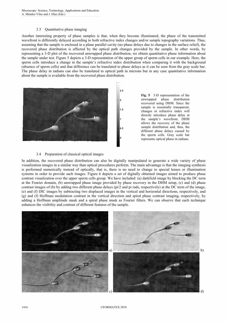
Fig. 5 3-D representation of the

unwrapped phase distribution

recovered using DHM. Since the

sample is essentially transparent,

changes in refractive index will

directly introduce phase delay at

the sample’s wavefront. DHM

allows the recovery of the phase

sample distribution and, thus, the

different phase delays caused by

the sperm cells. Gray scale bar

represents optical phase in radians.

3.3 Quantitative phase imaging

Another interesting property of phase samples is that, when they become illuminated, the phase of the transmitted

wavefront is differently delayed according to both refractive index changes and/or sample topography variations. Thus,

assuming that the sample is enclosed in a plane parallel cavity (no phase delays due to changes in the surface relief), the

recovered phase distribution is affected by the optical path changes provided by the sample. In other words, by

representing a 3-D plot of the recovered unwrapped phase distribution, we obtain quantitative phase information about

the sample under test. Figure 5 depicts a 3-D representation of the upper group of sperm cells in our example. Here, the

sperm cells introduce a change in the sample’s refractive index distribution when comparing it with the background

(absence of sperm cells) and that difference can be translated to phase delays as it can be seen from the gray scale bar.

The phase delay in radians can also be translated to optical path in microns but in any case quantitative information

about the sample is available from the recovered phase distribution.

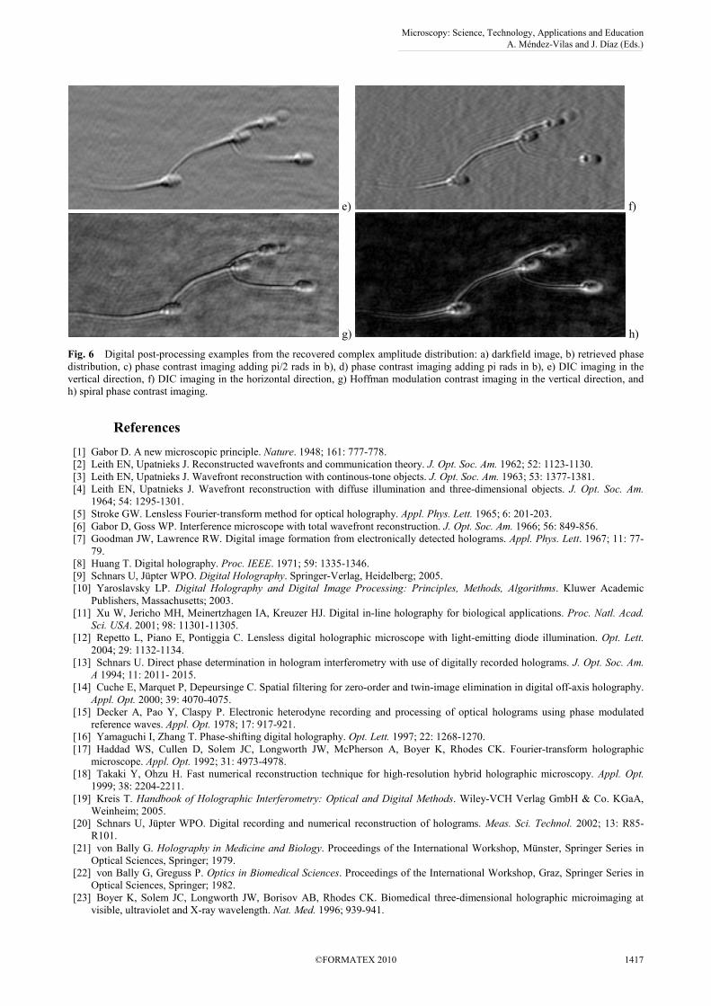
3.4 Preparation of classical optical images

In addition, the recovered phase distribution can also be digitally manipulated to generate a wide variety of phase

visualization images in a similar way than optical procedures perform. The main advantage is that the imaging synthesis

is performed numerically instead of optically, that is, there is no need to change to special lenses or illumination

systems in order to provide such images. Figure 6 depicts a set of digitally obtained images aimed to produce phase

contrast visualization over the upper sperm cells group. We have included: (a) darkfield image by blocking the DC term

at the Fourier domain, (b) unwrapped phase image provided by phase recovery in the DHM setup, (c) and (d) phase

contrast images of (b) by adding two different phase delays (pi/2 and pi rads, respectively) at the DC term of the image,

(e) and (f) DIC images by subtracting two displaced images in the vertical and horizontal directions, respectively, and

(g) and (f) Hoffman modulation contrast in the vertical direction and spiral phase contrast imaging, respectively, by

adding a Hoffman amplitude mask and a spiral phase mask as Fourier filters. We can observe that each technique

enhances the visibility and contrast of different features of the sample.

a) b)

c) d)



______________________________________________

e) f)

g) h)

Fig. 6 Digital post-processing examples from the recovered complex amplitude distribution: a) darkfield image, b) retrieved phase

distribution, c) phase contrast imaging adding pi/2 rads in b), d) phase contrast imaging adding pi rads in b), e) DIC imaging in the

vertical direction, f) DIC imaging in the horizontal direction, g) Hoffman modulation contrast imaging in the vertical direction, and

h) spiral phase contrast imaging.

References

[1] Gabor D. A new microscopic principle. Nature. 1948; 161: 777-778.

[2] Leith EN, Upatnieks J. Reconstructed wavefronts and communication theory. J. Opt. Soc. Am. 1962; 52: 1123-1130.

[3] Leith EN, Upatnieks J. Wavefront reconstruction with continous-tone objects. J. Opt. Soc. Am. 1963; 53: 1377-1381.

[4] Leith EN, Upatnieks J. Wavefront reconstruction with diffuse illumination and three-dimensional objects. J. Opt. Soc. Am. 1964; 54: 1295-1301.

[5] Stroke GW. Lensless Fourier‐transform method for optical holography. Appl. Phys. Lett. 1965; 6: 201-203.

[6] Gabor D, Goss WP. Interference microscope with total wavefront reconstruction. J. Opt. Soc. Am. 1966; 56: 849-856.

[7] Goodman JW, Lawrence RW. Digital image formation from electronically detected holograms. Appl. Phys. Lett. 1967; 11: 77-

79.

[8] Huang T. Digital holography. Proc. IEEE. 1971; 59: 1335-1346.

[9] Schnars U, Jüpter WPO. Digital Holography. Springer-Verlag, Heidelberg; 2005.

[10] Yaroslavsky LP. Digital Holography and Digital Image Processing: Principles, Methods, Algorithms. Kluwer Academic

Publishers, Massachusetts; 2003.

[11] Xu W, Jericho MH, Meinertzhagen IA, Kreuzer HJ. Digital in-line holography for biological applications. Proc. Natl. Acad. Sci. USA. 2001; 98: 11301-11305.

[12] Repetto L, Piano E, Pontiggia C. Lensless digital holographic microscope with light-emitting diode illumination. Opt. Lett. 2004; 29: 1132-1134.

[13] Schnars U. Direct phase determination in hologram interferometry with use of digitally recorded holograms. J. Opt. Soc. Am. A 1994; 11: 2011- 2015.

[14] Cuche E, Marquet P, Depeursinge C. Spatial filtering for zero-order and twin-image elimination in digital off-axis holography.

Appl. Opt. 2000; 39: 4070-4075.

[15] Decker A, Pao Y, Claspy P. Electronic heterodyne recording and processing of optical holograms using phase modulated

reference waves. Appl. Opt. 1978; 17: 917-921.

[16] Yamaguchi I, Zhang T. Phase-shifting digital holography. Opt. Lett. 1997; 22: 1268-1270.

[17] Haddad WS, Cullen D, Solem JC, Longworth JW, McPherson A, Boyer K, Rhodes CK. Fourier-transform holographic

microscope. Appl. Opt. 1992; 31: 4973-4978.

[18] Takaki Y, Ohzu H. Fast numerical reconstruction technique for high-resolution hybrid holographic microscopy. Appl. Opt. 1999; 38: 2204-2211.

[19] Kreis T. Handbook of Holographic Interferometry: Optical and Digital Methods. Wiley-VCH Verlag GmbH & Co. KGaA,

Weinheim; 2005.

[20] Schnars U, Jüpter WPO. Digital recording and numerical reconstruction of holograms. Meas. Sci. Technol. 2002; 13: R85-

R101.

[21] von Bally G. Holography in Medicine and Biology. Proceedings of the International Workshop, Münster, Springer Series in

Optical Sciences, Springer; 1979.

[22] von Bally G, Greguss P. Optics in Biomedical Sciences. Proceedings of the International Workshop, Graz, Springer Series in

Optical Sciences, Springer; 1982.

[23] Boyer K, Solem JC, Longworth JW, Borisov AB, Rhodes CK. Biomedical three-dimensional holographic microimaging at

visible, ultraviolet and X-ray wavelength. Nat. Med. 1996; 939-941.



______________________________________________

[24] Xu W, Jericho MH, Meinertzhagen IA, Kreuzer HJ. Tracking particles in 4-D with in-line holographic microscopy. Opt. Lett. 2003; 28: 164-166.

[25] Kanka M, Riesenberg R, Kreuzer HJ. Reconstruction of high-resolution holographic microscopic images. Opt. Lett. 2009; 34:

1162-1164.

[26] Zhang T, Yamaguchi I. Three-dimensional microscopy with phase-shifting digital holography. Opt. Lett. 1998; 23: 1221-1223.

[27] Cuche E, Marquet P, Depeursinge C. Simultaneous amplitude-contrast and quantitative phase-contrast microscopy by

numerical reconstruction of Fresnel off-axis holograms. Appl. Opt. 1999; 38: 6994-7001.

[28] Dubois F, Joannes L, Legros JC. Improved three-dimensional imaging with a digital holography microscope with a source of

partial spatial coherence. Appl. Opt. 1999; 38: 7085-7094.

[29] Colomb T, Dürr F, Cuche E, Marquet P, Limberger HG, Salathé RP, Depeursinge C. Polarization microscopy by use of digital

holography: application to optical-fiber birefringence measurements. Appl. Opt. 2005; 44: 4461-4469.

[30] Colomb T, Kühn J, Charrière F, Depeursinge C, Marquet P, Aspert N. Total aberrations compensation in digital holographic

microscopy with a reference conjugated hologram. Opt. Express 2006; 14: 4300-4306.

[31] Sheng J, Malkiel E, Katz J. Digital holographic microscope for measuring three-dimensional particle distributions and

motions. Appl. Opt. 2006; 45: 3893-3901.

[32] Ferraro P, Grilli S, Alfieri D, De Nicola S, Finizio A, Pierattini G, Javidi B, Coppola G, Striano V. Extended focused image in

microscopy by digital holography. Opt. Express 2005; 13: 6738-6749.

[33] Ferraro P, Coppola G, De Nicola S, Finizio A, Pierattini G. Digital holographic microscope with automatic focus tracking by

detecting sample displacement in real time. Opt. Lett. 2003; 28: 1257-1259.

[34] Marquet P, Rappaz B, Magistretti PJ, Cuche E, Emery Y, Colomb T, Depeursinge C. Digital holographic microscopy: a

noninvasive contrast imaging technique allowing quantitative visualization of living cells with subwavelength axial accuracy.

Opt. Lett. 2005; 30: 468-470.

[35] Dubois F, Minetti C, Monnom O, Yourassowsky C, Legros JC, Kischel P. Pattern recognition with a digital holographic

microscope working in partially coherent illumination. Appl. Opt. 2002; 41: 4108-4119.

[36] von Bally G, Kemper B, Carl D, Knoche S, Kempe M, Dietrich C, Stutz M, Wolleschensky R, Schütze K, Stich M,

Buchstaller A, Irion K, Beuthan J, Gersonde I, Schnekenburger J. New methods for marker-free live cell and tumor analysis (MIKROSO). Biophotonics: Visions for Better Health Care, J. Popp and M. Strehle, eds.; Wiley-VCH Verlag, pp. 301-360;

2006.

[37] Charrière F, Kühn J, Colomb T, Montfort F, Cuche E, Emery Y, Weible K, Marquet P, Depeursinge C. Characterization of

microlenses by digital holographic microscopy. Appl. Opt. 2006; 45: 829-835.

[38] Coppola G, Ferraro P, Iodice M, De Nicola S, Finizio A, Grilli S. A digital holographic microscope for complete

characterization of microelectromechanical systems. Meas. Sci. Technol. 2004; 15: 529-539.

[39] Rappaz B, Marquet P, Cuche E, Emery Y, Depeursinge C, Magistretti P. Measurement of the integral refractive index and

dynamic cell morphometry of living cells with digital holographic microscopy. Opt. Express 2005; 13: 9361-9373.

[40] Kemper B, von Bally G. Digital holographic microscopy for live cell applications and technical inspection. Appl. Opt. 2008;

47: A52-A61.

[41] Shi H, Fu Y, Quan C, Tay CJ, He X. Vibration measurement of a micro-structure by digital holographic microscopy. Meas. Sci. Technol. 2009; 20: 065301.

[42] Wahba HH, Kreis T. Characterization of graded index optical fibers by digital holographic interferometry. Appl. Opt. 2009;

48: 1573-1582.

[43] Iwai H, Fang-Yen C, Popescu G, Wax A, Badizadegan K, Dasari RR, Feld MS. Quantitative phase imaging using actively

stabilized phase-shifting low-coherence interferometry. Opt. Lett. 2004; 29: 2399-2401

[44] Reichelt S, Zappe H. Combined Twyman-Green and Mach-Zehnder interferometer for microlens testing. Appl. Opt. 2005; 44:

5786-5792.

[45] Mico V, Zalevsky Z, Garcia J. Common-path phase-shifting digital holographic microscopy: A way to quantitative phase

imaging and superresolution. Opt. Commun. 2008; 281: 4273-4281.

[46] Phase Holographic Imaging AB, Sweden, www.phiab.com

[47] Lyncée Tec SA, Switzerland, www.lynceetec.com

[48] Mico V, Garcia J, Zalevsky Z. Quantitative phase imaging by common-path interferometric microscopy: application to super-

resolved imaging and nanophotonics. J. Nanophoton. 2009; 3: 031780.

[49] Bernet S, Jesacher A, Fürhapter S, Maurer C, Ritsch-Marte M. Quantitative imaging of complex samples by spiral phase

contrast microscopy. Opt. Express. 2006; 14: 3792-3805.

[50] Popescu G, Deflores LP, Vaughan JC, Badizadegan K, Iwai H, Dasari RR, and Feld MS. Fourier phase microscopy for

investigation of biological structures and dynamics. Opt. Lett. 2004; 29: 2503-2505.

[51] Popescu G, Ikeda T, Dasari RR, and Feld MS. Diffraction phase microscopy for quantifying cell structure and dynamics. Opt. Lett. 2006; 31: 775-777.

[52] Ding H and Popescu G. Instantaneous spatial light interference microscopy. Opt. Express. 2010; 18: 1569-1575.



______________________________________________

basic principles and applications of digital holographic...

Documents