basic epidemiology teaching and learning pack -...
TRANSCRIPT

©LTPHN 2008 Original Author: Sarah Head Last Updated: 12/10/08
Basic Epidemiology Teaching and Learning Pack
Contents Title Type of resource
Introduction Tutor notes Tutorial 1 Disease frequency and measures of effect
Tutor notes
Tutorial 1 Disease frequency and measures of effect
Student notes
Tutorial 2 Bias
Tutor notes
Tutorial 2 Bias
Student notes
Tutorial 3 Causality
Tutor notes
Tutorial 3 Causality
Student notes
Tutorial 4 Study design
Tutor notes
Tutorial 4 Study design
Student notes

©LTPHN 2008 Original Author: Sarah Head Last Updated: 12/10/08
Title of Module: Basic Epidemiology
Type of resource: Tutor’s Notes
Author: Sarah Head
Subject expert: Paul Nelson
Date last updated: 12/10/08 By: Helen Barratt These resources are freely available to be copied and used for teaching and public health studies. Please acknowledge author and LTPHN for publication. ©LTPHN 2008

©LTPHN 2008 Original Author: Sarah Head Last Updated: 12/10/08
EPIDEMIOLOGY – TUTOR’S NOTES What will this module cover?
• Measurement – disease frequency and measures of effect) • Association – causation and the role of chance, bias and confounding • Study design
‘Epidemiology is the study of the distribution and determinants of health related states or events in specified populations, and the application of this study to control of health problems.’1 More simply it has been described as the ‘study of patterns of disease occurrence in human populations and the factors that influence these patterns.’2 History The word ‘epidemiology’ is derived from Greek word ‘Epidemos’ – ‘Epi’ meaning ‘upon’ and ‘demos’ meaning ‘the people’. It was used by Hippocrates to describe disease states that ‘visit the community.’ The word was first used in the English language in the 1850s – and originally referred to infectious disease outbreaks. In contrast, it now refers to studying patterns of all disease within the population – both infectious and non-infectious. Concepts involved Epidemiology examines how disease and determinants of disease are distributed at the population level.3 It is based upon two basic assumptions that:
a) Human disease does not occur randomly b) Human disease has causative and preventative factors, which can be identified by
examining how these factors vary in time, person and place within a population. Epidemiologists are interested in examining those without disease in order to compare them to those with disease. Done systematically, this leads to findings of what factors (e.g.. in time/person/place) are associated with a population developing the disease or remaining healthy. In turn this allows us to do put it to two main uses:
a) Public health - considering the knowledge supplied by epidemiology, to provide interventions at a population based level that will improve the overall health of the population
1 Last J. A Dictionary of Epidemiology. New York: Oxford University Press, 2001. 2 Lillienfeld A, Lillienfeld D. Foundations of Epidemiology. New York, Oxford University Press, 1980. 3 Hennekens CH, Buring JE. Epidemiology in medicine. Boston: Little, Brown and Company, 1987
©LTPHN 2008 Original Author: Sarah Head Last Updated: 12/10/08
b) Clinical work - using the knowledge supplied by epidemiology about risk factors for disease, health and related treatments to provide patients with an effective intervention in order to treat and prevent disease.
In essence, epidemiology is based upon three basic components to explore patterns of disease occurrence:
• Disease distribution in space (i.e. where?) • Disease distribution in time (i.e. when? how often?) • Disease determinants (i.e. what is associated? socioeconomic/lifestyle/drugs etc)
What can epidemiology be used for? • Understanding the natural history of a disease – for example, epidemiological studies of
hepatitis C have helped us understand that initial infection is generally asymptomatic, and approximately 80-85% of patients are left with chronic infection and may go on to develop cirrhosis.
• To describe patterns of disease – for example, concerning sources of HIV transmission, epidemiological techniques that have demonstrated that heterosexual transmission has become an increasingly important means of transmission in comparison to homosexual transmission and infected needles.
• Identify the cause of a new syndrome or even a new risk factor for a well described disease. For example, when the first cases of Severe Acute Respiratory Syndrome were recognised, even though it was laboratory techniques that eventually identified the organism, it was epidemiological techniques that provided information about the likely modes of transmission, risk factors, natural history etc of the disease.
• Assess the risks associated with a harmful exposure • Evaluation of a treatment/intervention – for example, epidemiological techniques are
used in trialling the effectiveness of a vaccine in preventing disease in a population. • Identifying health service use/needs/trends – for example, epidemiological studies of a
population form an essential part of a needs assessment, in order to estimate levels of need.
Why is epidemiology important? In addition to the above there are the following issues:
• Only by examining disease at the population level is it possible to truly identify an association. For example, not until the evidence at a population level was examined by Doll, was it possible to make a substantial case that smoking caused ill health. Without epidemiology, all we have are a collection of anecdotal reports.
• History has demonstrated that epidemiological techniques often uncover associations between determinants of disease and ill health before they can be demonstrated in laboratory studies. For example, epidemiology revealed the association between prone sleeping position and Sudden Infant Death Syndrome (SIDS), which in turn led to a change in health advice and decreased SIDS rates.
• Epidemiology helps us understand population health needs and is therefore important in planning health policy. For example, the changing epidemiology of TB in the UK
©LTPHN 2008 Original Author: Sarah Head Last Updated: 12/10/08
has resulted in the removal of the universal immunisation programme, and instead services now focus on high risk populations only.
• Understanding epidemiological techniques also allows us to appreciate the wider determinants of health. Epidemiological studies have shown clear socio-economic gradients in the uptake of breast cancer screening (women of lower socio-economic status are less likely to access screening). In addition to this, a recent study on breast cancer found that women living in deprived areas are more likely to have high grade/advanced stage breast cancer at diagnosis than women in more affluent areas.
Bias Definition ‘Any trend in the collection, analysis, interpretation, publication or review of data that can lead to conclusions that are systematically different from the truth’ – Lasts Dictionary of Epidemiology.
• Can occur to all types of study (though different study designs are more/less at risk of particular types of bias)
• Although difficult to avoid totally, can be minimised with careful planning of how study will be carried out.
• Number of different ways of classifying bias, but one of the best established is considering it as 2 main types
o Selection bias o Information bias
• Bias is a type of systematic error which (unlike confounding) cannot be adjusted for after the study has been carried out and the data has been collected.
Selection Bias This is bias that occurs as a result of errors during selection of the study population. Consequently, the relationship between the exposure and disease differs between those who were eligible to be enrolled in the study, and those who were actually enrolled. Selection bias can occur when: a) Differential surveillance/diagnosis/referral of patients into the study
• Cases may be more/less likely to be selected according to their exposure status. For example, when a link was first made between the Oral Contraceptive Pill (OCP) and thromboembolism, women presenting with symptoms of thromboembolism were more likely to be investigated if they were known to be on the OCP. Therefore, a case-control study using cases extracted from hospital records would demonstrate an exaggerated exposure to the OCP in relation to thromboembolism.
• Cases and controls sharing risk factors that may be related to developing outcome. For example, a case-control study of oral cancer and drinking. If the controls are drawn from a hospital population then they may be more likely drink than the general population and thus share risk factors for oral cancer. This would result in a decrease in the apparent risk of exposure on developing disease.
• Biased recruitment of patients into the study population. For example a GP asked to identify patients for a study on counselling and depression may only refer those
©LTPHN 2008 Original Author: Sarah Head Last Updated: 12/10/08
patients with milder disease who he feels will respond well to the treatment. This may lead to an exaggerated treatment effect of counselling.
b) Refusal/Non-response from cases or controls • Attempting to access controls by calling them at home during office hours will result
in a control group with high levels of non-working individuals whose age profiles may be older. This would not be a suitable control group if cases are mainly young working adults.
• Consider a case-control study on possible links between obesity and physical activity: ‘cases’ of obesity may refuse to be involved if they feel stigmatised.
c) Completeness of follow up • This is particularly relevant to cohort studies where individuals may be followed over
many years and subjects can consequently be lost to follow up. Although this may just occur by chance, it can also be related to the exposure or the outcome. If this varies between groups, then the results may be biased. For example, in a cohort study investigating the long term effects of an occupational exposure, subjects who become unwell (possibly as a result of the exposure of interest) may leave their job and become lost to follow up. This would give a biased estimate of the effect of the exposure.
Dealing with selection bias This varies depending on the individual situation but, in general, for methods to minimise selection bias in a case-control study include:
• Clearly defining the population of interest so that cases and controls can be extracted from exactly the same population
• Selecting controls from more than one source (e.g. hospital and community). There are pros and cons to using hospital controls vs. neighbourhood controls, so using both methods may compensate for weaknesses of one source.
• If there is concern about possible exposure as a source of bias, then additional information can be collected about this and the results analysed in separate strata.
Selection bias is a particular a problem for case-control studies because exposure and outcome have already occurred when the data is collected. In contrast, in cohort studies/RCTs, the outcome has not already occurred at the time of measurement of exposure status, and therefore knowledge of the patient’s outcome status cannot influence their enrolment in the study. Information Bias Information bias occurs when there is misclassification of the disease and/or the exposure status. This can occur in the following ways: a) Recall Bias
• In case-control studies in particular, where exposure status may be measured by an interview/questionnaire completed by the participant.
• Participants’ recall of their exposure may be dependent on their disease status: cases are often likely to overestimate exposures in comparison to controls. For example, in a case control study about congenital malformation and the use of medication during pregnancy, the mother of a case is more likely to remember any drugs she took in pregnancy than the mother of a control.
• In addition, people may under-report on sensitive issues (e.g. history of STD). • Use of proxies to gather information (e.g. interview with next of kin) may also result
in bias.

©LTPHN 2008 Original Author: Sarah Head Last Updated: 12/10/08
Additional sources of information such as prescriptions and patient records, can be used to minimise recall bias. b) Observer/Interviewer bias
• This occurs when those gathering information about the subjects introduce bias by the way they record/interpret the information.
• Knowledge of exposure status may influence classification of disease status, and knowledge of disease status may conversely influence classification of exposure status. For example, an interviewer collecting information for a case-control study about passive smoking and lung cancer may record a case as having a higher exposure status than a control.
• Observer bias does not only occur in interviews. It can also occur in situations such as taking measurements or extracting data from patient records.
Methods of minimising observer bias include blinding those collecting information to the status of participants, using rigorous study protocols and training of those collecting information. Additionally, using automated procedures such as an electronic blood pressure monitor rather than sphygnomometer, as well as validation of study techniques by external personnel, may also help.
©LTPHN 2008 Original Author: Sarah Head Last Updated: 12/10/08
Association and Causation In epidemiology we look for associations between exposure and outcome (e.g. inadequate folic acid in diet and neural tube defects). However, just because an apparent association has been found between exposure and outcome is not sufficient for implying causation. Firstly, not all associations will be true associations, and secondly association does not necessarily imply causation. For example, a study that demonstrates an apparent association between hypertension in pregnancy and low birthweight children may be
a) Only an apparent association, and in fact the result of systematic or random error b) A true association that occurs due to chance, rather than an exposure causing an
outcome c) A true relationship where hypertension causes low birthweight
Association is therefore very different to causation, and possible alternative explanations for an apparent association need to be carefully considered before causation is implied. Apparent association can be due to
a) Error • Random (i.e. chance finding) • Systematic (i.e. bias/confounding)
b) True Association If there is a true association between an exposure and outcome, this can be investigated further to explore if it is in fact causal. Therefore, in investigating causality, there are consequently two questions that need to be answered:
a) Is the association valid? Have chance, bias and confounding been eliminated? b) Is the association causal?
Investigating an apparent association This is the first step in investigating causality, and involves examination of the evidence to see if the observed association between an exposure and outcome is valid – i.e. is it a true association or just an apparent association? In order to do this both random and systematic error need to be excluded. Random error Chance variability may account for the results of a given study. Epidemiological studies cannot cover the whole population, so we use samples to try and represent these populations. Each sample taken from a population will vary slightly as a result of random variation. This chance variability can give rise to an apparent association between exposure and outcome, when in reality no true association exists (and vice versa). Although there is no definite way of proving whether this association has arisen by chance or not, statistical tests allow us assess how likely it is that this has arisen by chance. If it is deemed unlikely the finding had arisen by chance, this is termed a ‘statistically significant’ association. Systematic Error The apparent results of a study can arise from the way that a study is designed or conducted.

©LTPHN 2008 Original Author: Sarah Head Last Updated: 12/10/08
a) Bias - if there are differences in the way that study groups are selected or information is extracted from study groups, then this may affect the results of a study, for example showing an association between exposure and outcome where none exists (see above). b) Confounding – this is when a third (‘confounding’) factor affects the apparent association between the exposure and outcome. This variable is related independently to both the exposure and the outcome. Consequently the two associated exposures (the original exposure and the confounding factor) both affect the outcome, and the true association between the exposure of interest and the outcome is unclear. This relationship is best explained by Figure 1.
Figure 1: Socio-economic status as a confounder for the relationship between HRT use and breast cancer
Exposure Outcome (HRT use) (Breast Cancer)
Confounder (Socio-economic group)
Women of higher socio-economic group are more likely to use HRT and independently also more likely to develop breast cancer. Therefore, the result is that a study investigating the association between HRT and breast cancer, but not adjusting for socio-economic status as a confounder, could see a false increase in the apparent association between breast cancer and HRT use.
NB: Bias can only be addressed at the design stage of a study, and once it has occurred in a study nothing can be done to adjust for it. In contrast, confounding can be addressed at the both the design stage (by randomisation, restriction and matching) and the analysis stage (by stratification and statistical modelling). Once both random and systematic error have been excluded, there can be said to be a true association between exposure and outcome. However this does not necessarily imply causality.

©LTPHN 2008 Original Author: Sarah Head Last Updated: 12/10/08
Causality ‘A causal association is one in which a change in the frequency or quality of an exposure/characteristic results in a corresponding change in the frequency of disease or outcome of interest’ – taken from Hennekens p30 A judgment of causality needs to be made upon all available information, and re-evaluated in the light of any new findings. Bradford Hill Criteria These criteria to help evaluate whether an observed association is likely to be causal were first proposed in 1965 by the epidemiologist Austin Bradford Hill. They cannot prove causation but only suggest whether an association is likely.
1. Temporal sequence of association 2. Strength of association 3. Consistency of association (i.e. has it been observed in a number of different studies
on different populations?) 4. Biological gradient (i.e. dose-response relationship) 5. Specificity of association (this not always possible as an exposure is rarely associated
with a single outcome, and vice versa) 6. Plausibility of association 7. Coherence of association (i.e. it is in keeping with other current knowledge?) 8. Experimental evidence/reversibility 9. Other similar demonstrated associations (i.e. analogy)
Other additional features that have been suggested to help demonstrate causality include: • Prediction – i.e. assessing the predictive performance of a hypothesis • Alternate hypothesis – testing alternate hypotheses that could explain the same
observations
Koch’s postulates In 1882 the German physician and bacteriologist Robert Koch set out his celebrated criteria for judging whether a pathogen is the cause of a given disease. As they are related to a pathogen, they are generally only used for communicable diseases.
The pathogen (exposure) must meet 4 conditions:
1. It must be found in all cases of the disease 2. It must be isolated from the host and grown in pure culture 3. It must reproduce the original disease when introduced into a susceptible host 4. It must be found in the experimental host that was so infected
These criteria have been slightly expanded, for example to include features such as detection of a specific immune response, but in essence remain the same as above.
However, they do have limitations
• Some pathogens cannot be grown or are very difficult to grow in pure culture, for example Mycobacterium leprae and prions
• Some pathogens have no animal model to act as an experimental host

©LTPHN 2008 Original Author: Sarah Head Last Updated: 12/10/08
• An organism may cause disease in a human, but this may not show in an animal host Remember that causality is not a definite (proved/not proved) – the criteria above should only be used as guidelines. For further information/Resources Hennekens CH, Buring JE. Epidemiology in medicine. Boston: Little, Brown and Company, 1987 Beaglehole R, Bonita R, Kjellstrom T. Basic Epidemiology. Geneva: World Health Organization, 1993 Wald N. The Epidemiological Approach: An Introduction to Epidemiology in Medicine. London: Royal Society of Medicine/Wolfson Institute, 2004 MacMahon B, Trichopoulos D. Epidemiology, principles and methods. Boston: Little, Brown and Company, 1996. Coggon D, Rose G, Barker D. Epidemiology for the uninitiated (5th edition). London: British Medical Journal Publishing Group; 2002. Greenberg R, Daniels S, Flanders W, Eley J, Boring J. Medical epidemiology (3rd edition). New York, NY: Lange Medical Books, 2001 Fletcher R, Fletcher S, Wagner E. Clinical Epidemiology: The Essentials (3rd Edition). Baltimore: Lippincott Williams & Wilkins, 1996. Vetter N, Matthews I. Epidemiology and public health medicine. Edinburgh: Churchill Livingstone, 1999. Valanis B, Valanis B. Epidemiology in Health Care. New York: Appleton & Lange, 1999. Streiner D, Norman GR. PDQ Epidemiology. Hamilton: BC Decker, 1998. Timmreck T. An Introduction to Epidemiology. Boston: Jones and Bartlett, 1994.

©LTPHN 2008 Original Author: Sarah Head Last Updated: 12/10/08
Title of Module: Basic Epidemiology
Type of resource: Tutorial 1 – Tutor Version
Author: Sarah Head
Subject expert: Paul Nelson
Date last updated: 12/10/08 By: Helen Barratt
These resources are freely available to be copied and used for teaching and public health studies. Please acknowledge author and LTPHN for publication. ©LTPHN 2008

©LTPHN 2008 Original Author: Sarah Head Last Updated: 12/10/08
EPIDEMIOLOGY – TUTORIAL 1 DISEASE FREQUENCY & MEASURES OF EFFECT Quantifying the level of a disease 1. Examine the data in Table 1. What does this tell you about the levels of lung cancer in the
different towns?
Table 1
Town No. cases of lung cancer in 2007
A 10 B 100 C 1000
Discuss the pros and cons of using only this information, and what other data might be helpful and why. 2. What further information is given in Table 2? Why is this helpful?
Table 2
Town No. cases of lung cancer in 2007 Population Frequency of
disease A 10 1000 1/1000 B 100 1000 1/10 C 1000 100,000 1/1000
Measures of frequency 3. What methods do we have of expressing the frequency of a disease in relation to both
population and time? Ask the students to suggest ways of expressing disease frequency. If they use the words ‘incidence’ and ‘prevalence’ ask them to define them. If they do not, then discuss as per definitions below. 4. Examine the list of examples and discuss whether the figures are measurements of
prevalence or incidence • 12% of the 16-25yr old population are infected with chlamydia (Prevalence) • A study found 360 episodes of diarrhoea per 1000 children per year (Incidence) • 3% of the population of great Britain in 2004 have diabetes (Prevalence)
Discussion whether these represent incidence or prevalence.
• Incidence measures quantify the occurrence of new cases in a population • Prevalence quantifies existing cases in a population.
Figure 1: Definitions of Incidence/Prevalence

©LTPHN 2008 Original Author: Sarah Head Last Updated: 12/10/08
5. Table 3 illustrates the data required to calculate prevalence and incidence. What factors
might influence the observed prevalence rate of a disease?
Factors that increase the observed prevalence ratei • Longer duration of the disease • Prolongation of life of patients without cure • Increase in new cases (i.e. increase in incidence) • In migration of cases or susceptible people • Out migration of healthy people • Improved diagnostic facilities/surveillance etc.
Table 3 - Relationship of numerator/denominator to prevalence and incidenceii Incidence Prevalence
Numerator Number of new cases occurring during a defined period of time, amongst a group initially free of disease
Number of existing cases counted on a single survey or examination of a group
Denominator Total number of susceptible people present at the beginning of a period
Total number of people examined, including cases and non cases
Time Duration of the period (e.g. day/week/year) Single point in time
6. Which measure would provide the best estimate of the burden of a rare chronic disease in
a population? Why? Prevalence is better suited to stable conditions where it will represent the true frequency (i.e. if prevalence is measured at a single point in time for an unstable condition, the frequency of the condition may be inaccurately estimated). Compare situations of chronic/acute disease and rare/common disease. 7. What is the relationship between incidence and prevalence? Prevalence = Incidence x Average disease duration
Prevalence: The proportion of people in a defined population who have the disease under investigation at a fixed point in time Incidence The number of new cases of a disease occurring in a defined population during a specified time period.
©LTPHN 2008 Original Author: Sarah Head Last Updated: 12/10/08
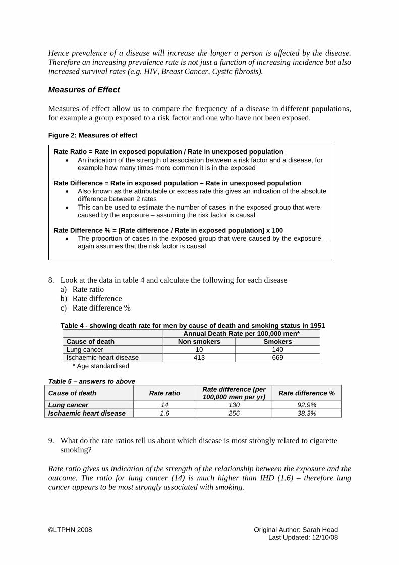
Hence prevalence of a disease will increase the longer a person is affected by the disease. Therefore an increasing prevalence rate is not just a function of increasing incidence but also increased survival rates (e.g. HIV, Breast Cancer, Cystic fibrosis). Measures of Effect Measures of effect allow us to compare the frequency of a disease in different populations, for example a group exposed to a risk factor and one who have not been exposed. Figure 2: Measures of effect
8. Look at the data in table 4 and calculate the following for each disease
a) Rate ratio b) Rate difference c) Rate difference %
Table 4 - showing death rate for men by cause of death and smoking status in 1951
Annual Death Rate per 100,000 men* Cause of death Non smokers Smokers Lung cancer 10 140 Ischaemic heart disease 413 669
* Age standardised Table 5 – answers to above
Cause of death Rate ratio Rate difference (per 100,000 men per yr) Rate difference %
Lung cancer 14 130 92.9% Ischaemic heart disease 1.6 256 38.3% 9. What do the rate ratios tell us about which disease is most strongly related to cigarette
smoking? Rate ratio gives us indication of the strength of the relationship between the exposure and the outcome. The ratio for lung cancer (14) is much higher than IHD (1.6) – therefore lung cancer appears to be most strongly associated with smoking.
Rate Ratio = Rate in exposed population / Rate in unexposed population • An indication of the strength of association between a risk factor and a disease, for
example how many times more common it is in the exposed Rate Difference = Rate in exposed population – Rate in unexposed population
• Also known as the attributable or excess rate this gives an indication of the absolute difference between 2 rates
• This can be used to estimate the number of cases in the exposed group that were caused by the exposure – assuming the risk factor is causal
Rate Difference % = [Rate difference / Rate in exposed population] x 100
• The proportion of cases in the exposed group that were caused by the exposure – again assumes that the risk factor is causal
©LTPHN 2008 Original Author: Sarah Head Last Updated: 12/10/08
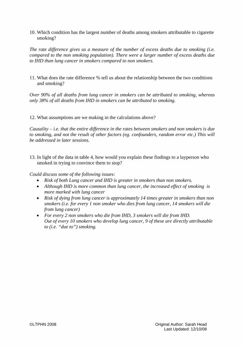
10. Which condition has the largest number of deaths among smokers attributable to cigarette smoking?
The rate difference gives us a measure of the number of excess deaths due to smoking (i.e. compared to the non smoking population). There were a larger number of excess deaths due to IHD than lung cancer in smokers compared to non smokers. 11. What does the rate difference % tell us about the relationship between the two conditions
and smoking? Over 90% of all deaths from lung cancer in smokers can be attributed to smoking, whereas only 38% of all deaths from IHD in smokers can be attributed to smoking. 12. What assumptions are we making in the calculations above? Causality – i.e. that the entire difference in the rates between smokers and non smokers is due to smoking, and not the result of other factors (eg. confounders, random error etc.) This will be addressed in later sessions. 13. In light of the data in table 4, how would you explain these findings to a layperson who
smoked in trying to convince them to stop? Could discuss some of the following issues:
• Risk of both Lung cancer and IHD is greater in smokers than non smokers. • Although IHD is more common than lung cancer, the increased effect of smoking is
more marked with lung cancer • Risk of dying from lung cancer is approximately 14 times greater in smokers than non
smokers (i.e. for every 1 non smoker who dies from lung cancer, 14 smokers will die from lung cancer)
• For every 2 non smokers who die from IHD, 3 smokers will die from IHD. Out of every 10 smokers who develop lung cancer, 9 of these are directly attributable to (i.e. “due to”) smoking.

©LTPHN 2008 Original Author: Sarah Head Last Updated: 12/10/08
Title of Module: Basic Epidemiology
Type of resource: Tutorial 1 – Student Version
Author: Sarah Head
Subject Expert: Paul Nelson
Date last updated: 12/10/08 By: Helen Barratt
These resources are freely available to be copied and used for teaching and public health studies. Please acknowledge author and LTPHN for publication. ©LTPHN 2008
©LTPHN 2008 Original Author: Sarah Head Last Updated: 12/10/08
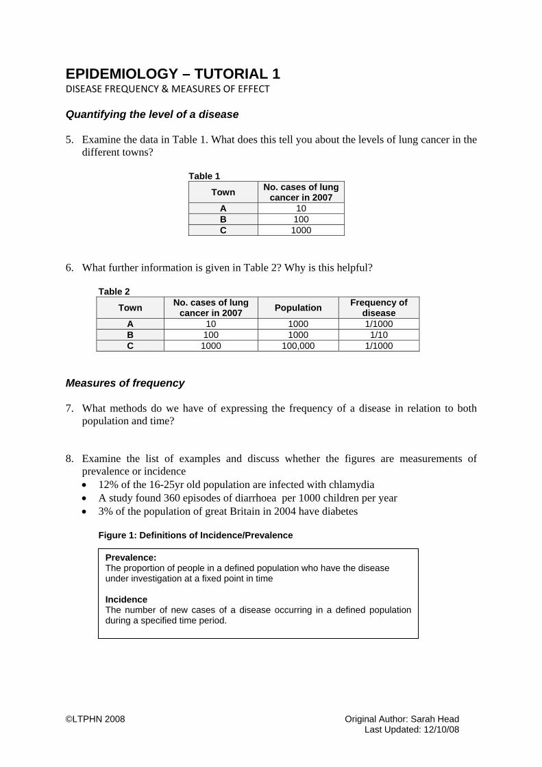
EPIDEMIOLOGY – TUTORIAL 1 DISEASE FREQUENCY & MEASURES OF EFFECT Quantifying the level of a disease 5. Examine the data in Table 1. What does this tell you about the levels of lung cancer in the
different towns?
Table 1
Town No. cases of lung cancer in 2007
A 10 B 100 C 1000
6. What further information is given in Table 2? Why is this helpful?
Table 2
Town No. cases of lung cancer in 2007 Population Frequency of
disease A 10 1000 1/1000 B 100 1000 1/10 C 1000 100,000 1/1000
Measures of frequency 7. What methods do we have of expressing the frequency of a disease in relation to both
population and time? 8. Examine the list of examples and discuss whether the figures are measurements of
prevalence or incidence • 12% of the 16-25yr old population are infected with chlamydia • A study found 360 episodes of diarrhoea per 1000 children per year • 3% of the population of great Britain in 2004 have diabetes
Figure 1: Definitions of Incidence/Prevalence
Prevalence: The proportion of people in a defined population who have the disease under investigation at a fixed point in time Incidence The number of new cases of a disease occurring in a defined population during a specified time period.
©LTPHN 2008 Original Author: Sarah Head Last Updated: 12/10/08
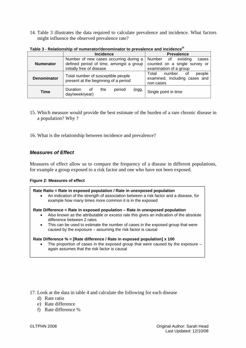
14. Table 3 illustrates the data required to calculate prevalence and incidence. What factors might influence the observed prevalence rate?
Table 3 - Relationship of numerator/denominator to prevalence and incidenceiii Incidence Prevalence
Numerator Number of new cases occurring during a defined period of time, amongst a group initially free of disease
Number of existing cases counted on a single survey or examination of a group
Denominator Total number of susceptible people present at the beginning of a period
Total number of people examined, including cases and non cases
Time Duration of the period (egg. day/week/year) Single point in time
15. Which measure would provide the best estimate of the burden of a rare chronic disease in
a population? Why ? 16. What is the relationship between incidence and prevalence? Measures of Effect Measures of effect allow us to compare the frequency of a disease in different populations, for example a group exposed to a risk factor and one who have not been exposed. Figure 2: Measures of effect
17. Look at the data in table 4 and calculate the following for each disease
d) Rate ratio e) Rate difference f) Rate difference %
Rate Ratio = Rate in exposed population / Rate in unexposed population • An indication of the strength of association between a risk factor and a disease, for
example how many times more common it is in the exposed Rate Difference = Rate in exposed population – Rate in unexposed population
• Also known as the attributable or excess rate this gives an indication of the absolute difference between 2 rates
• This can be used to estimate the number of cases in the exposed group that were caused by the exposure – assuming the risk factor is causal
Rate Difference % = [Rate difference / Rate in exposed population] x 100
• The proportion of cases in the exposed group that were caused by the exposure – again assumes that the risk factor is causal

©LTPHN 2008 Original Author: Sarah Head Last Updated: 12/10/08
Table 4 - showing death rate for men by cause of death and smoking status in 1951 Annual Death Rate per 100,000 men* Cause of death Non smokers Smokers Lung cancer 10 140 Ischaemic heart disease 413 669
* Age standardised Table 5 – answers to above
Cause of death Rate ratio Rate difference (per 100,000 men per yr) Rate difference %
Lung cancer
Ischaemic heart disease
18. What do the rate ratios tell us about which disease is most strongly related to cigarette
smoking? 19. Which condition has the largest number of deaths among smokers attributable to cigarette
smoking? 20. What does the rate difference % tell us about the relationship between the two conditions
and smoking? 21. What assumptions are we making in the calculations above? 22. In light of the data in table 4, how would you explain these findings to a layperson who
smoked in trying to convince them to stop?

©LTPHN 2008 Original Author: Sarah Head Last Updated: 12/10/08
Title of Module: Basic Epidemiology
Type of resource: Tutorial 2 – Tutor Version
Author: Sarah Head
Subject expert: Paul Nelson
Date last updated: 12/10/08 By: Helen Barratt These resources are freely available to be copied and used for teaching and public health studies. Please acknowledge author and LTPHN for publication. ©LTPHN 2008

©LTPHN 2008 Original Author: Sarah Head Last Updated: 12/10/08
EPIDEMIOLOGY – TUTORIAL 2
BIAS Read the extract in Figure 1, and then answer the following questions. 1. What do you understand by bias? Answers will give an indication of how much of the separate tutor notes you need to discuss with the group before progressing to rest of tutorial. 2. What type of study is this? Case control study 3. Bias in identifying the cases and controls is known as selection bias. From the
information given in the methods, comment on factors that may have a) reduced bias and b) been a source of bias in the selection of cases and controls
Reducing bias
• Clearly defined entry criteria for cases and controls (with use of preset algorithm to ensure systematic approach)
• Variety of different sources used to select cases (i.e. hospital, cancer registries etc) so representative of true disease population
• Most of the population are registered with a GP so characteristics of controls are representative of the wider population that the diseased group comes from.
• Attempt was made to ensure that the cases/controls had similar profiles for age/sex/location
Increasing bias
• Some of population are not registered with a GP (for example homeless, asylum seekers etc). This group likely to have poor health outcomes and probably less likely to have a mobile phone. Therefore control population not truly representative of whole population
• GP registers may not be up to date due to presence of “ghosts” – hence this may lead to participation bias (i.e. controls contacted from GP records may not live in that area any more so will not respond to invitation).
• We are told that “Non-participating controls were replaced” but it is unclear exactly how. i.e. – if the protocol was not used for this, then could be influenced by GP/consultant – hence introducing bias.
• Also, we are not told (in this extract – although is written in full study) how many of those invited to participate refused.
©LTPHN 2008 Original Author: Sarah Head Last Updated: 12/10/08
4. If the controls were all hospital patients, how might this have affected the results of the study? What conditions would have to be met to minimise bias in the selection of controls in this situation?
A control population of hospital patients are more likely to have poor health outcomes and may share risk factors for the disease in question. Little is currently known about the aetiology of gliomas so this would be difficult to assess. The result of choosing a control population in this way is likely to reduce the apparent effect of the exposure on the outcome. Bias could be minimised if care was taken to select a population which was representative of the case population (e.g. age/sex) but was known not to have any excessive risk factors for glioma. Since little is currently known about aetiology of gliomas this would be difficult to do. 5. The results section tells us that:
Overall response rates were 51% for patients with glioma and 45% for controls, representing the proportion of all eligible cases and controls from the study areas who were interviewed in the study
Do you think this could affect the study? If so, how? Participation rates were poor for both controls and cases. Controls who agreed to participate may have been unrepresentative of the true population pool (i.e. those who responded to invitation may be in a different socio-economic group, have different lifestyles, more/less likely to own a mobile phone etc) Cases may also be unrepresentative of all patients with the disease for the same reasons. In addition, non response of cases may be due to some having already died due to a more aggressive form of disease. If this were the case, the study might fail to identify a true association between mobile phone use and aggressive forms of the disease (but not less aggressive forms).
6. What could the investigators have done to see if the response rates had resulted in biased
results? Examine the characteristics of non-responders (e.g. grade of glioma at diagnosis). This way a comparison could be made between responders and non- responders to confirm if the groups were similar. If they appear to be similar, it is less likely that the results are biased by the low participation rates. This may best be explained by Fig 2. Students may also answer in response to this that study design could have been changed to improve uptake rates of participants. Although this does not answer the question directly it could lead to a useful discussion around methods of improving uptake rates in a study e.g. clear information, follow up by phone/letter/person, accurate address details, incentives etc 7. How was information on exposure status (mobile phone use) collected? What type of bias
may this have caused in the study?
©LTPHN 2008 Original Author: Sarah Head Last Updated: 12/10/08
Collected by interview – with detailed questions on mobile phone use. This was dependant on accurate recall so may be at risk of Recall &Reporting bias. Ways in which this can manifest include:
• Participants may not remember information at all • Participants may remember information incorrectly • Participants may give answers that are influenced by the knowledge that they
do/don’t have glioma 8. Some information had to be collected by proxy interviews. Comment on how this may
have biased the results Similar to above (q.7) – also more difficult to report accurately on someone else’s mobile phone use. Consider how difficult it would be for you to answer detailed questions on how a friend/relative used their mobile phone. In addition - the spouse of a person with glioma may be prone to overestimate how much their spouse used a mobile – since they may suspect there is a relationship between mobile phone use and glioma. 9. Interviews can be susceptible to observer bias. Can you explain how, and how this may
be overcome? Observer bias can occur in interviews: • Interviewer may ask questions in a slightly different way for each subject, so influencing
answers given. This is overcome by using highly structured interviews with closed questions, and careful training of interviewers (e.g. “ How much did you use your mobile phone in the past month?” Vs “ For how many hours did you use your mobile phone last month? 0-5/6-10/11-15/16+”)
• Interviewer may unknowingly prompt participant one direction or another if the interviewer is aware whether they participant is a case or not. This is overcome by blinding interviewers and external validation of interviews.
• Interviewer may make subject feel inhibited such that they provide answers they consider to be socially acceptable (more relevant with sensitive topics etc. e.g. Questions on how many sexual parters, hx of termination of pregnancy etc). This can be overcome by using carefully ordered questions (i.e. start off with v neutral, leading to more sensitive questions later in interview), careful training/selection of interviewers, use of computer self interview (rather than personal interviewer)
For all of the above, careful training and selection of interviewers, together with clear protocols, is important in reducing bias. Additional questions: 10. The results of this study demonstrate that over 80% of cases and controls had used/ been
exposed to a mobile phone for less than 5years. Therefore, if an association was found between developing a glioma and having mobile phone exposure, what assumption would have to be made concerning the temporal relationship between exposure and outcome?
11. Is this the best type of study design to answer this question – can you suggest one more suitable?
This can lead to discussions about causality (including the temporal relationship between exposure and outcome) and choice of study design.

©LTPHN 2008 Original Author: Sarah Head Last Updated: 12/10/08
• In order to agree that there was a true causal relationship between exposure to mobile phones and outcome of glioma, we would need to assume that the time from exposure to mobile phone and diagnosis of glioma is less than 5 years. Knowledge of most temporal relationships for exposure and outcome (particularly environmental/occupational hazards) tells us that exposure to development of disease would normally takes much longer than this, for example smoking and lung cancer. See rapid response by Kundi for more details
• To demonstrate a temporal relationship, a cohort study may be more suitable than a case control study. However from the other perspective, glioma is a rare outcome and for this reason a case control study is suitable.
©LTPHN 2008 Original Author: Sarah Head Last Updated: 12/10/08
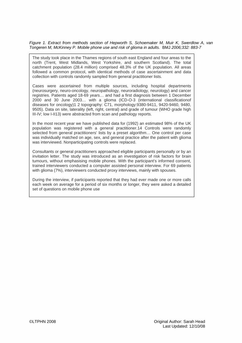
Figure 1. Extract from methods section of Hepworth S, Schoemaker M, Muir K, Swerdlow A, van Tongeren M, McKinney P. Mobile phone use and risk of glioma in adults. BMJ 2006;332: 883-7
The study took place in the Thames regions of south east England and four areas to the north (Trent, West Midlands, West Yorkshire, and southern Scotland). The total catchment population (28.4 million) comprised 48.3% of the UK population. All areas followed a common protocol, with identical methods of case ascertainment and data collection with controls randomly sampled from general practitioner lists. Cases were ascertained from multiple sources, including hospital departments (neurosurgery, neuro-oncology, neuropathology, neuroradiology, neurology) and cancer registries. Patients aged 18-69 years… and had a first diagnosis between 1 December 2000 and 30 June 2003… with a glioma (ICD-O-3 (international classificationof diseases for oncology)1 2 topography: C71, morphology:9380-9411, 9420-9460, 9480, 9505). Data on site, laterality (left, right, central) and grade of tumour (WHO grade high III-IV; low I-II13) were abstracted from scan and pathology reports. In the most recent year we have published data for (1992) an estimated 98% of the UK population was registered with a general practitioner.14 Controls were randomly selected from general practitioners’ lists by a preset algorithm… One control per case was individually matched on age, sex, and general practice after the patient with glioma was interviewed. Nonparticipating controls were replaced. Consultants or general practitioners approached eligible participants personally or by an invitation letter. The study was introduced as an investigation of risk factors for brain tumours, without emphasising mobile phones. With the participant’s informed consent, trained interviewers conducted a computer assisted personal interview. For 69 patients with glioma (7%), interviewers conducted proxy interviews, mainly with spouses. During the interview, if participants reported that they had ever made one or more calls each week on average for a period of six months or longer, they were asked a detailed set of questions on mobile phone use

Figure 2. The effects of poor participation on study bias
Investigate the characteristics of non-participants e.g. sex, socio-economic status, health status etc
Participation rates similar in both cases and controls
Poor participation of cases and controls in study
Participation rates differ between case and control groups
Non-participants similar to cases and controls
Non-participants differ from cases and controls
Outcome less likely to be biased but generalisability may be affected
Outcome likely to be affected by bias

Title of Module: Basic Epidemiology
Type of resource: Tutorial 2 – Student Version
Author: Sarah Head
Subject expert: Paul Nelson
Date last updated: 12/10/08 By: Helen Barratt These resources are freely available to be copied and used for teaching and public health studies. Please acknowledge author and LTPHN for publication. ©LTPHN 2008

Basic Epidemiology – Tutorial 2
©LTPHN 2008 Original Author: Sarah Head Last Updated: 12/10/08
EPIDEMIOLOGY – TUTORIAL 2 BIAS Read the extract in Figure 1, and then answer the following questions. 10. What do you understand by bias? 11. What type of study is this? 12. Bias in identifying the cases and controls is known as selection bias. From the
information given in the methods, comment on factors that may have a) reduced bias and b) been a source of bias in the selection of cases and controls
13. If the controls were all hospital patients, how might this have affected the results
of the study? What conditions would have to be met to minimise bias in the selection of controls in this situation?
14. The results section tells us that:
Overall response rates were 51% for patients with glioma and 45% for controls, representing the proportion of all eligible cases and controls from the study areas who were interviewed in the study
Do you think this could affect the study? If so, how?
15. What could the investigators have done to see if the response rates had resulted in
biased results? 16. How was information on exposure status (mobile phone use) collected? What type
of bias may this have caused in the study? 17. Some information had to be collected by proxy interviews. Comment on how this
may have biased the results 18. Interviews can be susceptible to observer bias. Can you explain how, and how this
may be overcome?

Basic Epidemiology – Tutorial 2
©LTPHN 2008 Original Author: Sarah Head Last Updated: 12/10/08
Additional questions: 12. The results of this study demonstrate that over 80% of cases and controls had
used/ been exposed to a mobile phone for less than 5years. Therefore, if an association was found between developing a glioma and having mobile phone exposure, what assumption would have to be made concerning the temporal relationship between exposure and outcome?
13. Is this the best type of study design to answer this question – can you suggest one
more suitable?

Basic Epidemiology – Tutorial 2
©LTPHN 2008 Original Author: Sarah Head Last Updated: 12/10/08
Figure 1. Extract from methods section of Hepworth S, Schoemaker M, Muir K, Swerdlow A, van Tongeren M, McKinney P. Mobile phone use and risk of glioma in adults. BMJ 2006;332: 883-7
The study took place in the Thames regions of south east England and four areas to the north (Trent, West Midlands, West Yorkshire, and southern Scotland). The total catchment population (28.4 million) comprised 48.3% of the UK population. All areas followed a common protocol, with identical methods of case ascertainment and data collection with controls randomly sampled from general practitioner lists. Cases were ascertained from multiple sources, including hospital departments (neurosurgery, neuro-oncology, neuropathology, neuroradiology, neurology) and cancer registries. Patients aged 18-69 years… and had a first diagnosis between 1 December 2000 and 30 June 2003… with a glioma (ICD-O-3 (international classificationof diseases for oncology)1 2 topography: C71, morphology:9380-9411, 9420-9460, 9480, 9505). Data on site, laterality (left, right, central) and grade of tumour (WHO grade high III-IV; low I-II13) were abstracted from scan and pathology reports. In the most recent year we have published data for (1992) an estimated 98% of the UK population was registered with a general practitioner.14 Controls were randomly selected from general practitioners’ lists by a preset algorithm… One control per case was individually matched on age, sex, and general practice after the patient with glioma was interviewed. Nonparticipating controls were replaced. Consultants or general practitioners approached eligible participants personally or by an invitation letter. The study was introduced as an investigation of risk factors for brain tumours, without emphasising mobile phones. With the participant’s informed consent, trained interviewers conducted a computer assisted personal interview. For 69 patients with glioma (7%), interviewers conducted proxy interviews, mainly with spouses. During the interview, if participants reported that they had ever made one or more calls each week on average for a period of six months or longer, they were asked a detailed set of questions on mobile phone use

Basic Epidemiology – Tutorial 2
©LTPHN 2008 Original Author: Sarah Head Last Updated: 12/10/08
Figure 2. The effects of poor participation on study bias i Beaglehole R, Bonita R, Kjellstrom T. Basic Epidemiology. Geneva: WHO, 1993 ii Fletcher R, Fletcher S, Wagner E. Clinical Epidemiology: The Essentials. Baltimore: Lippincott Williams & Wilkins, 1996 (3rd Edition) iii Fletcher R, Fletcher S, Wagner E. Clinical Epidemiology: The Essentials. Baltimore: Lippincott Williams & Wilkins, 1996 (3rd Edition)
Investigate the characteristics of non-participants egg. sex, socio-economic status, health status etc
Participation rates similar in both cases and controls
Poor participation of cases and controls in study
Participation rates differ between case and control groups
Non-participants similar to cases and controls
Non-participants differ from cases and controls
Outcome less likely to be biased but generalisability may be affected
Outcome likely to be affected by bias
Basic Epidemiology – Tutorial 2
©LTPHN 2008 Original Author: Sarah Head Last Updated: 12/10/08
Title of Module: Basic Epidemiology
Type of resource: Tutorial 3 –Tutor Version
Author: Sarah Head
Subject expert: Paul Nelson
Date last updated: 12/10/08 By: Helen Barratt These resources are freely available to be copied and used for teaching and public health studies. Please acknowledge author and LTPHN for publication. ©LTPHN 2008

Basic Epidemiology – Tutorial 2
©LTPHN 2008 Original Author: Sarah Head Last Updated: 12/10/08
EPIDEMIOLOGY – TUTORIAL 3 CAUSALITY When students are carrying out this tutorial, it is important to remember that causality is not a definite (i.e. proved/not proved) – there are areas of grey and the criteria are only used as guidelines. Therefore it is important to maintain an open approach to students’ responses and not try to complete the list as a ‘tick box’ exercise. 1. Why is it widely believed that smoking causes lung cancer? See what answers students give. Even if have no knowledge of Bradford Hill Criteria some of the answers they give should meet them. This can then lead onto a discussion around Bradford Hill Criteria. If students already have knowledge then discuss how these criteria are met by the smoking and lung cancer argument. If students mention Koch criteria – explain that this will be discussed in q.2 – and that usually thought of in terms of a communicable disease. Bradford Hill Criteria for smoking and lung cancer
• Strength of Association –the case-control study carried out by Doll and Peto showed a strong positive association between smoking and lung cancer. This was followed by other similar studies that demonstrated similar results. They showed approximately a 10 fold association in risk of developing lung cancer in current smokers.
• Temporality – the cohort study of British Doctors was the main evidence demonstrating that populations who smoked went on to develop lung cancer
• Consistency – the above results have been replicated in a number of different studies in different populations, including the USA and UK
• Biological gradient – evidence from case control studies shows that heavy smokers have up to a 20x increase in lung cancer, compared to a 10x increase in lung cancer in standard current smokers.
• Experimental evidence/reversibility – ex-smokers have been found to have consistently lower risks of developing lung cancer than current smokers. With increasing time these risks decrease, all they do not fall to the level of an individual who has never smoked.
• Specificity – this is one criteria that is not really met – since it is known that smoking does not just cause lung cancer but a wide range of other diseases as well (e.g. COPD, oral cancer). Similarly, lung cancer has other cause in addition to smoking – e.g. asbestos exposure.
• Plausibility of association – studies identified over 200 compounds in cigarette smoke that are known to be carcinogens/cocarcinogens/cancer promoters. This provided biological evidence to support the association.
• Coherence of association – numerous studies support this. • Other similar demonstrated associations (i.e. analogy) e.g. Smoking and cancer of
mouth, soot and scrotal cancer.
Basic Epidemiology – Tutorial 2
©LTPHN 2008 Original Author: Sarah Head Last Updated: 12/10/08
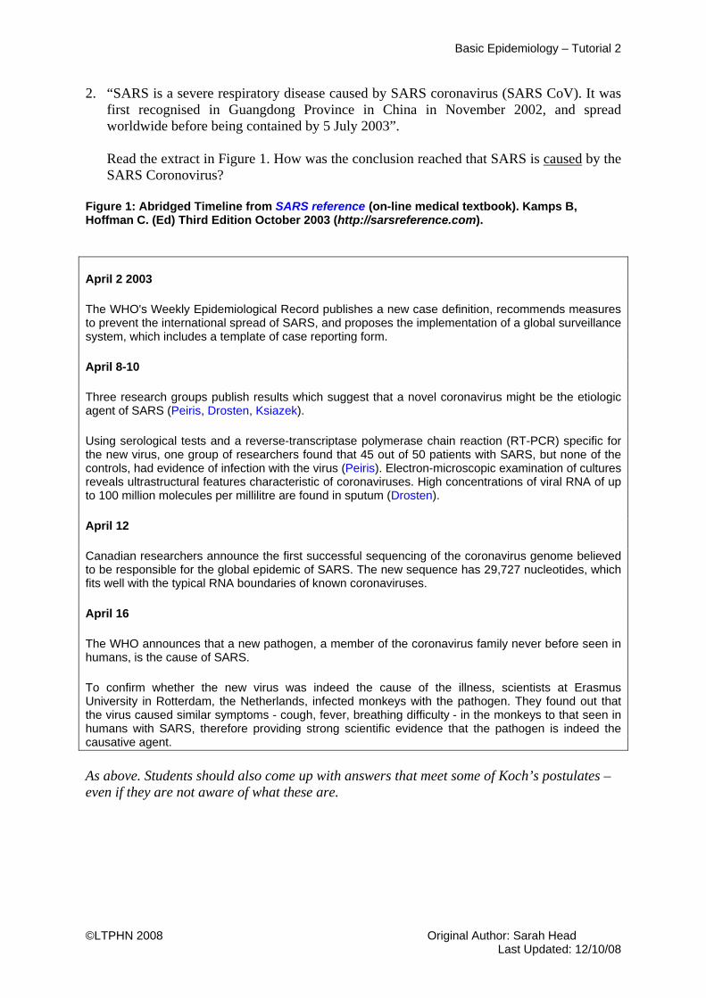
2. “SARS is a severe respiratory disease caused by SARS coronavirus (SARS CoV). It was first recognised in Guangdong Province in China in November 2002, and spread worldwide before being contained by 5 July 2003”.
Read the extract in Figure 1. How was the conclusion reached that SARS is caused by the SARS Coronovirus?
Figure 1: Abridged Timeline from SARS reference (on-line medical textbook). Kamps B, Hoffman C. (Ed) Third Edition October 2003 (http://sarsreference.com). April 2 2003
The WHO's Weekly Epidemiological Record publishes a new case definition, recommends measures to prevent the international spread of SARS, and proposes the implementation of a global surveillance system, which includes a template of case reporting form.
April 8-10
Three research groups publish results which suggest that a novel coronavirus might be the etiologic agent of SARS (Peiris, Drosten, Ksiazek).
Using serological tests and a reverse-transcriptase polymerase chain reaction (RT-PCR) specific for the new virus, one group of researchers found that 45 out of 50 patients with SARS, but none of the controls, had evidence of infection with the virus (Peiris). Electron-microscopic examination of cultures reveals ultrastructural features characteristic of coronaviruses. High concentrations of viral RNA of up to 100 million molecules per millilitre are found in sputum (Drosten).
April 12
Canadian researchers announce the first successful sequencing of the coronavirus genome believed to be responsible for the global epidemic of SARS. The new sequence has 29,727 nucleotides, which fits well with the typical RNA boundaries of known coronaviruses.
April 16
The WHO announces that a new pathogen, a member of the coronavirus family never before seen in humans, is the cause of SARS.
To confirm whether the new virus was indeed the cause of the illness, scientists at Erasmus University in Rotterdam, the Netherlands, infected monkeys with the pathogen. They found out that the virus caused similar symptoms - cough, fever, breathing difficulty - in the monkeys to that seen in humans with SARS, therefore providing strong scientific evidence that the pathogen is indeed the causative agent.
As above. Students should also come up with answers that meet some of Koch’s postulates – even if they are not aware of what these are.

Basic Epidemiology – Tutorial 2
©LTPHN 2008 Original Author: Sarah Head Last Updated: 12/10/08
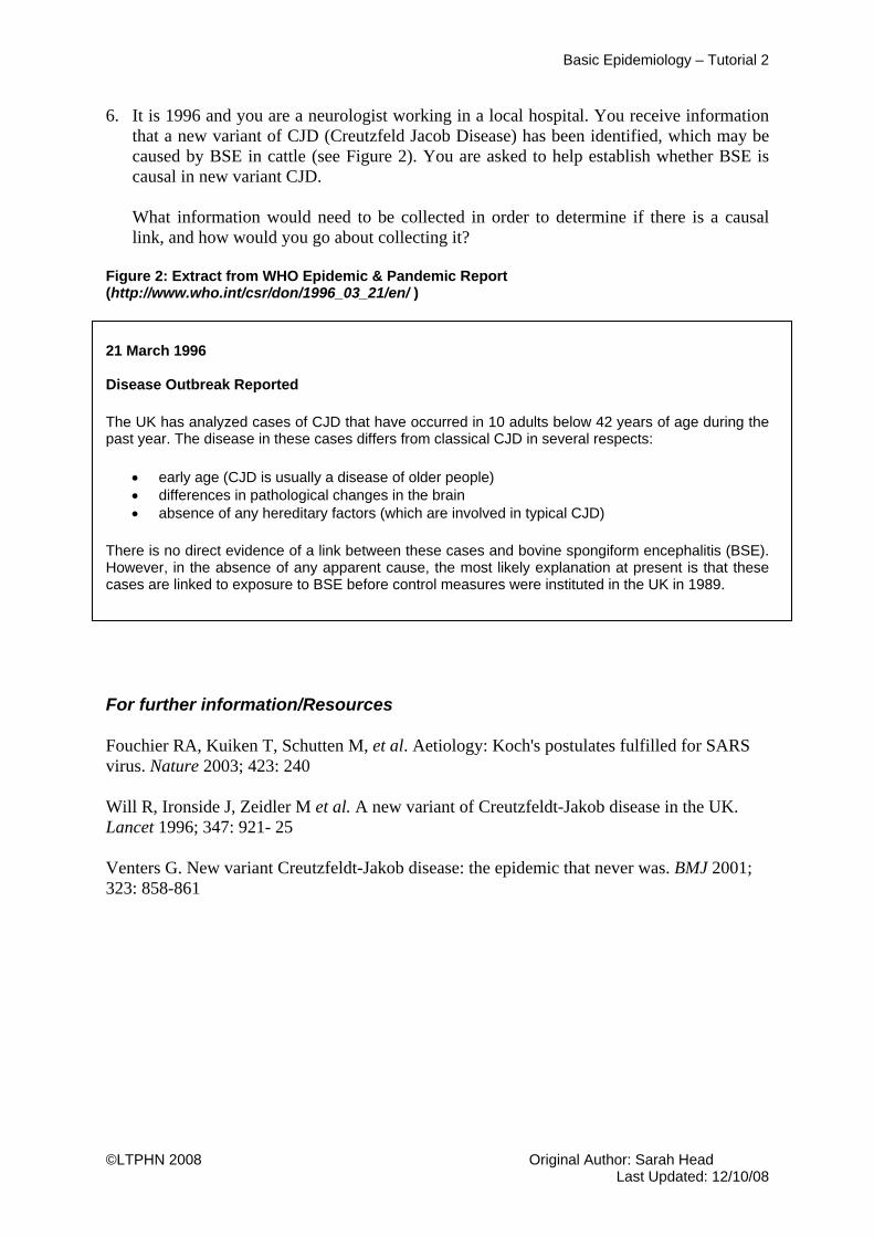
3. It is 1996 and you are a neurologist working in a local hospital. You receive information that a new variant of CJD (Creutzfeld Jacob Disease) has been identified, which may be caused by BSE in cattle (see Figure 2). You are asked to help establish whether BSE is causal in new variant CJD.
What information would need to be collected in order to determine if there is a causal link, and how would you go about collecting it?
Figure 2: Extract from WHO Epidemic & Pandemic Report (http://www.who.int/csr/don/1996_03_21/en/)
21 March 1996 Disease Outbreak Reported
The UK has analyzed cases of CJD that have occurred in 10 adults below 42 years of age during the past year. The disease in these cases differs from classical CJD in several respects:
• early age (CJD is usually a disease of older people) • differences in pathological changes in the brain • absence of any hereditary factors (which are involved in typical CJD)
There is no direct evidence of a link between these cases and bovine spongiform encephalitis (BSE). However, in the absence of any apparent cause, the most likely explanation at present is that these cases are linked to exposure to BSE before control measures were instituted in the UK in 1989. Really this is a further revision of the criteria of causality, but also considering research methods. It should also help students to see the value of epidemiology.
Information needed:
- Case definition of the “ new disease” - Information to answer questions raised by causal frameworks i.e. Bradford
Hill/Koch’s postulates. - Understanding of BSE and why it may be biologically plausible that it is causal in
vCJD How information collected to answer above
- “Case definition” from expert knowledge/initial studies - Establishing a surveillance system (current and retrospective) over the area
concerned in order to collect data about possible cases that meet the case definition.
- Setting up epidemiological studies – could discuss pros/cons of different types e.g. i. Case control study – to investigate association between BSE (and other
possible risk factors) and new variant CJD ii. Cohort study to investigate association and look for temporal relationship
iii. RCT – not possible due to ethics! - Laboratory studies to test Koch’s postulates (though difficult to test reproduction
of disease in host since appeared to be human specific, and this is not ethical!!) - Investigate existing evidence on BSE

Basic Epidemiology – Tutorial 2
©LTPHN 2008 Original Author: Sarah Head Last Updated: 12/10/08
For further information/Resources
Fouchier RA, Kuiken T, Schutten M, et al. Aetiology: Koch's postulates fulfilled for SARS virus. Nature 2003; 423: 240
Will R, Ironside J, Zeidler M et al. A new variant of Creutzfeldt-Jakob disease in the UK. Lancet 1996; 347: 921- 25
Venters G. New variant Creutzfeldt-Jakob disease: the epidemic that never was. BMJ 2001; 323: 858-861

Basic Epidemiology – Tutorial 2
©LTPHN 2008 Original Author: Sarah Head Last Updated: 12/10/08
Title of Module: Basic Epidemiology
Type of resource: Tutorial 3 – Student Version
Author: Sarah Head
Subject expert: Paul Nelson
Date last updated: 12/10/08 By: Helen Barratt These resources are freely available to be copied and used for teaching and public health studies. Please acknowledge author and LTPHN for publication. ©LTPHN 2008

Basic Epidemiology – Tutorial 2
©LTPHN 2008 Original Author: Sarah Head Last Updated: 12/10/08
EPIDEMIOLOGY – TUTORIAL 3 CAUSALITY 4. Why is it widely believed that smoking causes lung cancer? 5. “SARS is a severe respiratory disease caused by SARS coronavirus (SARS CoV). It was
first recognised in Guangdong Province in China in November 2002, and spread worldwide before being contained by 5 July 2003.”
Read the extract in Figure 1. How was the conclusion reached that SARS is caused by the SARS Coronovirus?
Figure 1: Abridged Timeline from SARS reference (on-line medical textbook). Kamps B, Hoffman C. (Ed) Third Edition October 2003 (http://sarsreference.com). April 2 2003
The WHO's Weekly Epidemiological Record publishes a new case definition, recommends measures to prevent the international spread of SARS, and proposes the implementation of a global surveillance system, which includes a template of case reporting form.
April 8-10
Three research groups publish results which suggest that a novel coronavirus might be the etiologic agent of SARS (Peiris, Drosten, Ksiazek).
Using serological tests and a reverse-transcriptase polymerase chain reaction (RT-PCR) specific for the new virus, one group of researchers found that 45 out of 50 patients with SARS, but none of the controls, had evidence of infection with the virus (Peiris). Electron-microscopic examination of cultures reveals ultrastructural features characteristic of coronaviruses. High concentrations of viral RNA of up to 100 million molecules per millilitre are found in sputum (Drosten).
April 12
Canadian researchers announce the first successful sequencing of the coronavirus genome believed to be responsible for the global epidemic of SARS. The new sequence has 29,727 nucleotides, which fits well with the typical RNA boundaries of known coronaviruses.
April 16
The WHO announces that a new pathogen, a member of the coronavirus family never before seen in humans, is the cause of SARS.
To confirm whether the new virus was indeed the cause of the illness, scientists at Erasmus University in Rotterdam, the Netherlands, infected monkeys with the pathogen. They found out that the virus caused similar symptoms - cough, fever, breathing difficulty - in the monkeys to that seen in humans with SARS, therefore providing strong scientific evidence that the pathogen is indeed the causative agent.
Basic Epidemiology – Tutorial 2
©LTPHN 2008 Original Author: Sarah Head Last Updated: 12/10/08
6. It is 1996 and you are a neurologist working in a local hospital. You receive information that a new variant of CJD (Creutzfeld Jacob Disease) has been identified, which may be caused by BSE in cattle (see Figure 2). You are asked to help establish whether BSE is causal in new variant CJD.
What information would need to be collected in order to determine if there is a causal link, and how would you go about collecting it?
Figure 2: Extract from WHO Epidemic & Pandemic Report (http://www.who.int/csr/don/1996_03_21/en/ )
21 March 1996 Disease Outbreak Reported
The UK has analyzed cases of CJD that have occurred in 10 adults below 42 years of age during the past year. The disease in these cases differs from classical CJD in several respects:
• early age (CJD is usually a disease of older people) • differences in pathological changes in the brain • absence of any hereditary factors (which are involved in typical CJD)
There is no direct evidence of a link between these cases and bovine spongiform encephalitis (BSE). However, in the absence of any apparent cause, the most likely explanation at present is that these cases are linked to exposure to BSE before control measures were instituted in the UK in 1989.
For further information/Resources
Fouchier RA, Kuiken T, Schutten M, et al. Aetiology: Koch's postulates fulfilled for SARS virus. Nature 2003; 423: 240
Will R, Ironside J, Zeidler M et al. A new variant of Creutzfeldt-Jakob disease in the UK. Lancet 1996; 347: 921- 25
Venters G. New variant Creutzfeldt-Jakob disease: the epidemic that never was. BMJ 2001; 323: 858-861

Basic Epidemiology – Tutorial 2
©LTPHN 2008 Original Author: Sarah Head Last Updated: 12/10/08
Title of Module: Basic Epidemiology
Type of resource: Tutorial 4 – Tutor Version
Author: Sarah Head
Subject expert: Paul Nelson
Date last updated: 12/10/08 By: Helen Barratt These resources are freely available to be copied and used for teaching and public health studies. Please acknowledge author and LTPHN for publication. ©LTPHN 2008
Basic Epidemiology – Tutorial 2
©LTPHN 2008 Original Author: Sarah Head Last Updated: 12/10/08
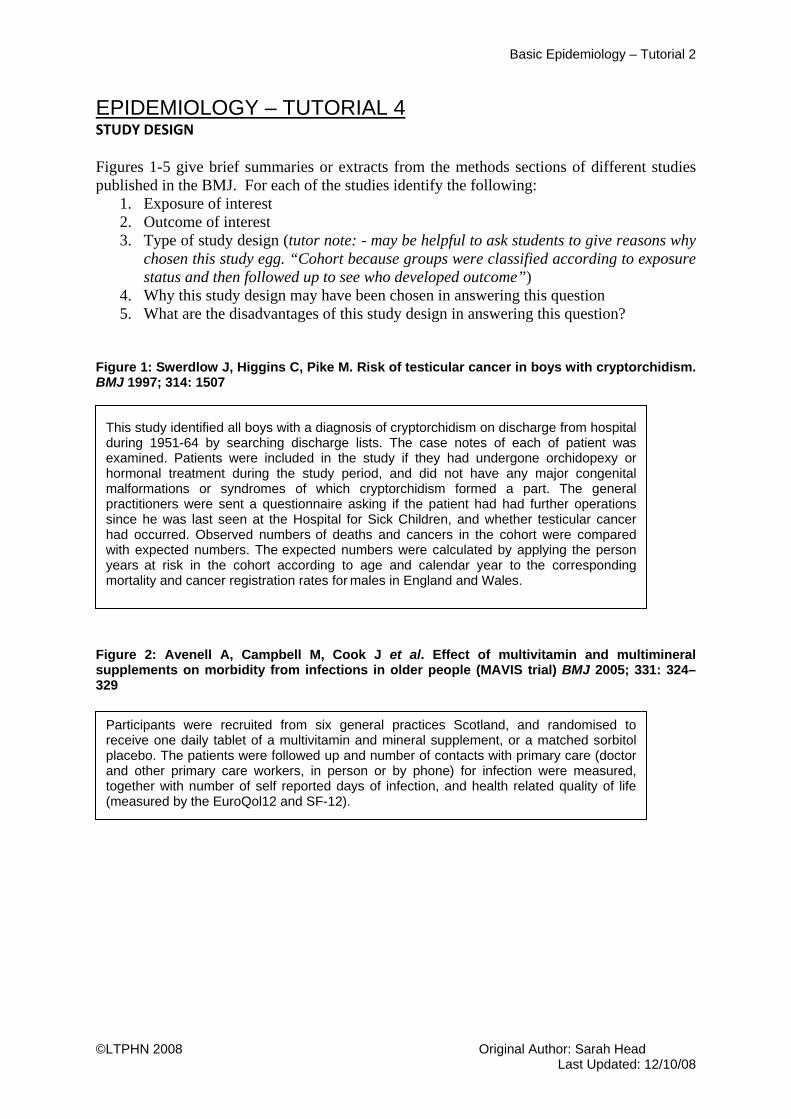
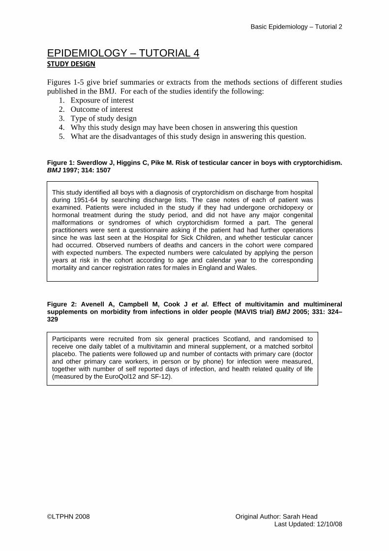
EPIDEMIOLOGY – TUTORIAL 4 STUDY DESIGN Figures 1-5 give brief summaries or extracts from the methods sections of different studies published in the BMJ. For each of the studies identify the following:
1. Exposure of interest 2. Outcome of interest 3. Type of study design (tutor note: - may be helpful to ask students to give reasons why
chosen this study egg. “Cohort because groups were classified according to exposure status and then followed up to see who developed outcome”)
4. Why this study design may have been chosen in answering this question 5. What are the disadvantages of this study design in answering this question?
Figure 1: Swerdlow J, Higgins C, Pike M. Risk of testicular cancer in boys with cryptorchidism. BMJ 1997; 314: 1507 Figure 2: Avenell A, Campbell M, Cook J et al. Effect of multivitamin and multimineral supplements on morbidity from infections in older people (MAVIS trial) BMJ 2005; 331: 324–329
This study identified all boys with a diagnosis of cryptorchidism on discharge from hospital during 1951-64 by searching discharge lists. The case notes of each of patient was examined. Patients were included in the study if they had undergone orchidopexy or hormonal treatment during the study period, and did not have any major congenital malformations or syndromes of which cryptorchidism formed a part. The general practitioners were sent a questionnaire asking if the patient had had further operations since he was last seen at the Hospital for Sick Children, and whether testicular cancer had occurred. Observed numbers of deaths and cancers in the cohort were compared with expected numbers. The expected numbers were calculated by applying the person years at risk in the cohort according to age and calendar year to the corresponding mortality and cancer registration rates for males in England and Wales.
Participants were recruited from six general practices Scotland, and randomised to receive one daily tablet of a multivitamin and mineral supplement, or a matched sorbitol placebo. The patients were followed up and number of contacts with primary care (doctor and other primary care workers, in person or by phone) for infection were measured, together with number of self reported days of infection, and health related quality of life (measured by the EuroQol12 and SF-12).

Basic Epidemiology – Tutorial 2
©LTPHN 2008 Original Author: Sarah Head Last Updated: 12/10/08
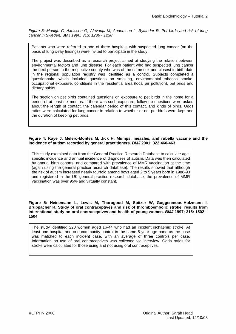
Figure 3: Modigh C, Axelsson G, Alavanja M, Andersson L, Rylander R. Pet birds and risk of lung cancer in Sweden. BMJ 1996; 313: 1236 - 1238 Figure 4: Kaye J, Melero-Montes M, Jick H. Mumps, measles, and rubella vaccine and the incidence of autism recorded by general practitioners. BMJ 2001; 322:460-463
Figure 5: Heinemann L, Lewis M, Thorogood M, Spitzer W, Guggenmoos-Holzmann I, Bruppacher R. Study of oral contraceptives and risk of thromboembolic stroke: results from international study on oral contraceptives and health of young women. BMJ 1997; 315: 1502 – 1504
This study examined data from the General Practice Research Database to calculate age-specific incidence and annual incidence of diagnoses of autism. Data was then calculated by annual birth cohorts, and compared with prevalence of MMR vaccination at the time (again using the general practice research database). The results showed that although the risk of autism increased nearly fourfold among boys aged 2 to 5 years born in 1988-93 and registered in the UK general practice research database, the prevalence of MMR vaccination was over 95% and virtually constant.
The study identified 220 women aged 16-44 who had an incident ischaemic stroke. At least one hospital and one community control in the same 5 year age band as the case was matched to each incident case, with an average of three controls per case. Information on use of oral contraceptives was collected via interview. Odds ratios for stroke were calculated for those using and not using oral contraceptives.
Patients who were referred to one of three hospitals with suspected lung cancer (on the basis of lung x-ray findings) were invited to participate in the study. The project was described as a research project aimed at studying the relation between environmental factors and lung disease. For each patient who had suspected lung cancer the next person in the respective county who was of the same sex and closest in birth date in the regional population registry was identified as a control. Subjects completed a questionnaire which included questions on smoking, environmental tobacco smoke, occupational exposure, conditions in the residential area (local air pollution), pet birds and dietary habits. The section on pet birds contained questions on exposure to pet birds in the home for a period of at least six months. If there was such exposure, follow up questions were asked about the length of contact, the calendar period of this contact, and kinds of birds. Odds ratios were calculated for lung cancer in relation to whether or not pet birds were kept and the duration of keeping pet birds.
Basic Epidemiology – Tutorial 2
©LTPHN 2008 Original Author: Sarah Head Last Updated: 12/10/08
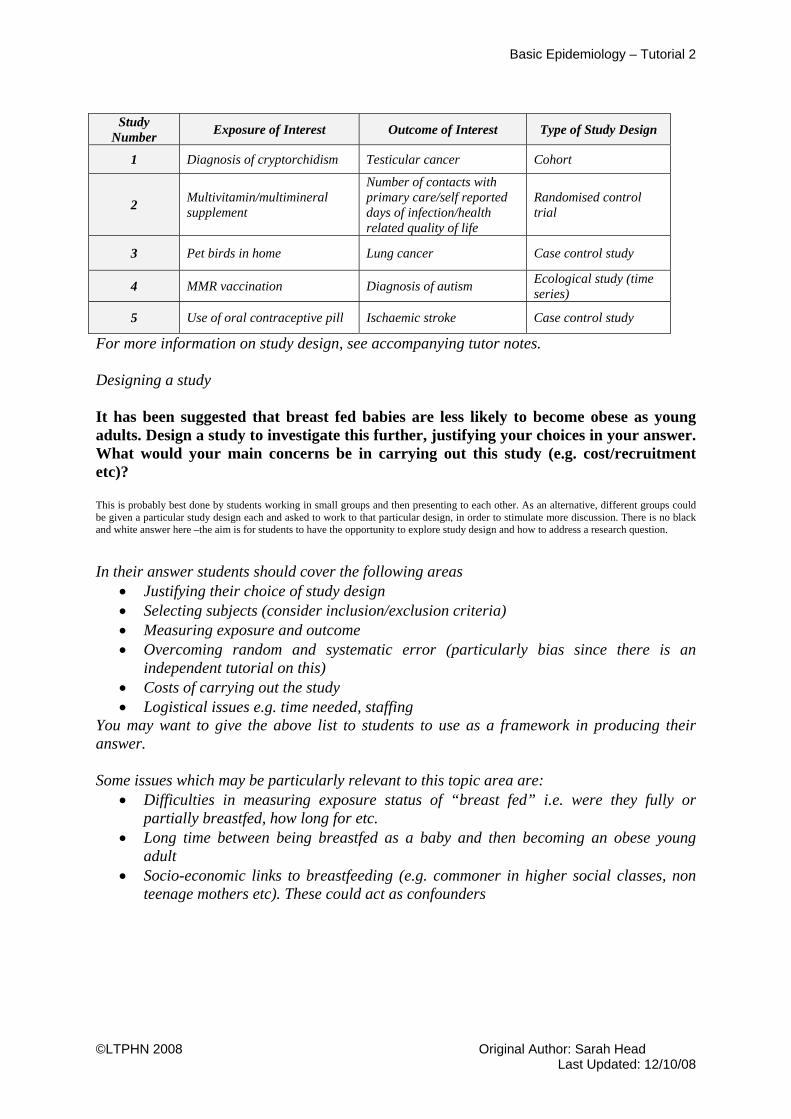
Study
Number Exposure of Interest Outcome of Interest Type of Study Design
1 Diagnosis of cryptorchidism Testicular cancer Cohort
2 Multivitamin/multimineral supplement
Number of contacts with primary care/self reported days of infection/health related quality of life
Randomised control trial
3 Pet birds in home Lung cancer Case control study
4 MMR vaccination Diagnosis of autism Ecological study (time series)
5 Use of oral contraceptive pill Ischaemic stroke Case control study
For more information on study design, see accompanying tutor notes. Designing a study It has been suggested that breast fed babies are less likely to become obese as young adults. Design a study to investigate this further, justifying your choices in your answer. What would your main concerns be in carrying out this study (e.g. cost/recruitment etc)? This is probably best done by students working in small groups and then presenting to each other. As an alternative, different groups could be given a particular study design each and asked to work to that particular design, in order to stimulate more discussion. There is no black and white answer here –the aim is for students to have the opportunity to explore study design and how to address a research question.
In their answer students should cover the following areas
• Justifying their choice of study design • Selecting subjects (consider inclusion/exclusion criteria) • Measuring exposure and outcome • Overcoming random and systematic error (particularly bias since there is an
independent tutorial on this) • Costs of carrying out the study • Logistical issues e.g. time needed, staffing
You may want to give the above list to students to use as a framework in producing their answer. Some issues which may be particularly relevant to this topic area are:
• Difficulties in measuring exposure status of “breast fed” i.e. were they fully or partially breastfed, how long for etc.
• Long time between being breastfed as a baby and then becoming an obese young adult
• Socio-economic links to breastfeeding (e.g. commoner in higher social classes, non teenage mothers etc). These could act as confounders

Basic Epidemiology – Tutorial 2
©LTPHN 2008 Original Author: Sarah Head Last Updated: 12/10/08
For further information/Resources Li L, Parsons T, Power C. Breast feeding and obesity in childhood: cross sectional study. BMJ 2003; 327: 904 - 905 von Kries R, Koletzko B, Sauerwald T et al. Breast feeding and obesity: cross sectional study BMJ 1999; 319: 147 - 150 Parsons TJ, Power C, Manor O. Infant feeding and obesity through the lifecourse. Arch Dis Child 2003; 88: 793-4. Victora C, Barros F, Lima R, Horta B, Wells J. Anthropometry and body composition of 18 year old men according to duration of breast feeding: birth cohort study from Brazil. BMJ 2003 327: 901. Dewey K. Is breastfeeding protective against child obesity? J Hum Lact 2003;19: 9-18

Basic Epidemiology – Tutorial 2
©LTPHN 2008 Original Author: Sarah Head Last Updated: 12/10/08
Title of Module: Basic Epidemiology
Type of resource: Tutorial 4 – Student Version
Author: Sarah Head
Subject expert: Paul Nelson
Date last updated: 12/10/08 By: Helen Barratt These resources are freely available to be copied and used for teaching and public health studies. Please acknowledge author and LTPHN for publication. ©LTPHN 2008
Basic Epidemiology – Tutorial 2
©LTPHN 2008 Original Author: Sarah Head Last Updated: 12/10/08
EPIDEMIOLOGY – TUTORIAL 4 STUDY DESIGN Figures 1-5 give brief summaries or extracts from the methods sections of different studies published in the BMJ. For each of the studies identify the following:
1. Exposure of interest 2. Outcome of interest 3. Type of study design 4. Why this study design may have been chosen in answering this question 5. What are the disadvantages of this study design in answering this question.
Figure 1: Swerdlow J, Higgins C, Pike M. Risk of testicular cancer in boys with cryptorchidism. BMJ 1997; 314: 1507 Figure 2: Avenell A, Campbell M, Cook J et al. Effect of multivitamin and multimineral supplements on morbidity from infections in older people (MAVIS trial) BMJ 2005; 331: 324–329
This study identified all boys with a diagnosis of cryptorchidism on discharge from hospital during 1951-64 by searching discharge lists. The case notes of each of patient was examined. Patients were included in the study if they had undergone orchidopexy or hormonal treatment during the study period, and did not have any major congenital malformations or syndromes of which cryptorchidism formed a part. The general practitioners were sent a questionnaire asking if the patient had had further operations since he was last seen at the Hospital for Sick Children, and whether testicular cancer had occurred. Observed numbers of deaths and cancers in the cohort were compared with expected numbers. The expected numbers were calculated by applying the person years at risk in the cohort according to age and calendar year to the corresponding mortality and cancer registration rates for males in England and Wales.
Participants were recruited from six general practices Scotland, and randomised to receive one daily tablet of a multivitamin and mineral supplement, or a matched sorbitol placebo. The patients were followed up and number of contacts with primary care (doctor and other primary care workers, in person or by phone) for infection were measured, together with number of self reported days of infection, and health related quality of life (measured by the EuroQol12 and SF-12).
Basic Epidemiology – Tutorial 2
©LTPHN 2008 Original Author: Sarah Head Last Updated: 12/10/08
Figure 3: Modigh C, Axelsson G, Alavanja M, Andersson L, Rylander R. Pet birds and risk of lung cancer in Sweden. BMJ 1996; 313: 1236 - 1238 Figure 4: Kaye J, Melero-Montes M, Jick H. Mumps, measles, and rubella vaccine and the incidence of autism recorded by general practitioners. BMJ 2001; 322:460-463
Figure 5: Heinemann L, Lewis M, Thorogood M, Spitzer W, Guggenmoos-Holzmann I, Bruppacher R. Study of oral contraceptives and risk of thromboembolic stroke: results from international study on oral contraceptives and health of young women. BMJ 1997; 315: 1502 – 1504
This study examined data from the General Practice Research Database to calculate age-specific incidence and annual incidence of diagnoses of autism. Data was then calculated by annual birth cohorts, and compared with prevalence of MMR vaccination at the time (again using the general practice research database). The results showed that although the risk of autism increased nearly fourfold among boys aged 2 to 5 years born in 1988-93 and registered in the UK general practice research database, the prevalence of MMR vaccination was over 95% and virtually constant.
The study identified 220 women aged 16-44 who had an incident ischaemic stroke. At least one hospital and one community control in the same 5 year age band as the case was matched to each incident case, with an average of three controls per case. Information on use of oral contraceptives was collected via interview. Odds ratios for stroke were calculated for those using and not using oral contraceptives.
Patients who were referred to one of three hospitals with suspected lung cancer (on the basis of lung x-ray findings) were invited to participate in the study. The project was described as a research project aimed at studying the relation between environmental factors and lung disease. For each patient who had suspected lung cancer the next person in the respective county who was of the same sex and closest in birth date in the regional population registry was identified as a control. Subjects completed a questionnaire which included questions on smoking, environmental tobacco smoke, occupational exposure, conditions in the residential area (local air pollution), pet birds and dietary habits. The section on pet birds contained questions on exposure to pet birds in the home for a period of at least six months. If there was such exposure, follow up questions were asked about the length of contact, the calendar period of this contact, and kinds of birds. Odds ratios were calculated for lung cancer in relation to whether or not pet birds were kept and the duration of keeping pet birds.
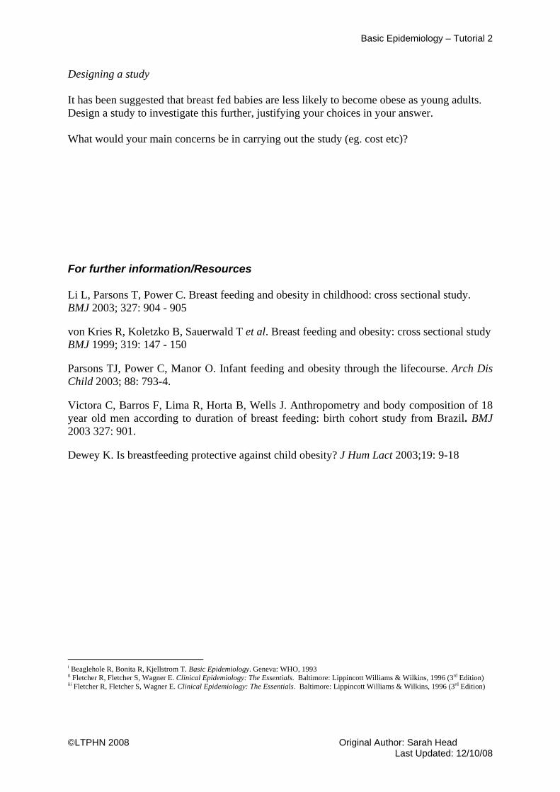
Basic Epidemiology – Tutorial 2
©LTPHN 2008 Original Author: Sarah Head Last Updated: 12/10/08
Designing a study It has been suggested that breast fed babies are less likely to become obese as young adults. Design a study to investigate this further, justifying your choices in your answer. What would your main concerns be in carrying out the study (eg. cost etc)? For further information/Resources Li L, Parsons T, Power C. Breast feeding and obesity in childhood: cross sectional study. BMJ 2003; 327: 904 - 905 von Kries R, Koletzko B, Sauerwald T et al. Breast feeding and obesity: cross sectional study BMJ 1999; 319: 147 - 150 Parsons TJ, Power C, Manor O. Infant feeding and obesity through the lifecourse. Arch Dis Child 2003; 88: 793-4. Victora C, Barros F, Lima R, Horta B, Wells J. Anthropometry and body composition of 18 year old men according to duration of breast feeding: birth cohort study from Brazil. BMJ 2003 327: 901. Dewey K. Is breastfeeding protective against child obesity? J Hum Lact 2003;19: 9-18 i Beaglehole R, Bonita R, Kjellstrom T. Basic Epidemiology. Geneva: WHO, 1993 ii Fletcher R, Fletcher S, Wagner E. Clinical Epidemiology: The Essentials. Baltimore: Lippincott Williams & Wilkins, 1996 (3rd Edition) iii Fletcher R, Fletcher S, Wagner E. Clinical Epidemiology: The Essentials. Baltimore: Lippincott Williams & Wilkins, 1996 (3rd Edition)