Basic Data Manipulation

SAC (Seismic Analysis Code)

General purpose interactive program designed for the study of sequential signals,

especially seismic timeseries data (seismograms).

Emphasis has been placed on analysis tools used by research seismologists in the

detailed study of seismic events.

SAC (Seismic Analysis Code) Analysis capabilities include:

- General arithmetic operations - Fourier transforms

-  integration/differentiation - spectral estimation/processing techniques

- IIR and FIR filtering - Signal stacking

-  Decimation and Interpolation, -  Correlation,

-  seismic phase (time and amplitude) picking -  Instrument correction -  Particle motion rotation

-  Trace envelopes -  Linear regressions

-  Frequency-wavenumber analysis -  various types of plotting.

SAC (Seismic Analysis Code)

SAC also contains an extensive graphics capability.

(for the early 1980’s.)

SAC

Seismic Analysis Code was developed at Lawrence Livermore National Laboratory (LLNL) and University of California in the

early 1980's.

LLNL is one of the 3 US Nuclear weapons laboratories.

Seismology is one of the principle tools in Nuclear Test Ban treaty verification.

SAC

SAC was developed using PRIME Microcomputers under the PRIMEOS.

It was written in FORTRAN.

SAC

It is a command-driven, as opposed to a menu or GUI driven, program.

It took advantage of several features of the PRIMEOS, such as its command line

processor that passes commands that are not part of the program to the OS.

(This means, that if one is running SAC and you need to get a directory listing, you just enter the “ls” command. Since this is not a SAC command, the command

line processor will pass the command to the OS and you will get a directory listing. You don’t have to leave SAC, do the “ls”, write down/remember the file

name, and restart SAC. This was very important in the pre –GUI days.)

SAC

Although it can run in batch mode, it was principally designed to be interactive and

have interactive graphics.

It was designed to use the “state-of-the-art” Tektronix 401X “storage tube” line of

graphics terminals.

Tektronix 4010 Specifications Data Transfer Rate: 150 to 9600 baud Screen Size: 8 1/4 by 6 3/8 inches Character Set : UPPER CASE ONLY 63 total 5x7 matrix Format : 74 characters per line 35 lines per screen (2590 characters) Character Draw Time: 1200 per second Vector Resolution: 1024 by 780 Vector Draw Time: 2.6 milliseconds maximum Usable Storage Time: Up to one hour without permanent damage Operating Environment: 10 to 40 C (50-104F) Power: 192 watts maximum Weight: 78 pounds

Notice the blistering speed -

Data Transfer Rate: 150 to 9600 baud.

This will come back to haunt us.

SAC

After the demise of PRIME in the early 90’s, SAC was beaten into submission to run under

the UNIX operating system, specifically, SOLARIS, the SUN OS.

(as with UNIX, it dragged along many of the idiosyncrasies of its birth associated with the PRIMEOS and the hardware limitations of the time – such

as the TEK401X. The UNIX implementation was the simplest “make it run” under UNIX effort.)

It now runs on most UNIX/LINUX systems and has become one of the standard data

manipulation tools in seismology.

SAC

SAC’s data format, especially for binary data, is one of the principle data formats used today in storing, transferring, and

manipulating (earthquake) seismological time series data.

SAC’s competitors (analysis) include

- IRIS/PASSCAL AH system

- Various versions (with various names) of DATASCOPE (now Antelope)

- XPICK

- Seismic UNIX

-  MATSEIS

-  others

SAC’s competitors (data format) include

AH (Ad Hoc, used by IRIS/PASSCAL program)

SEED (Standard for the Exchange of Earthquake Data, native format IRIS-DMC)

CSS (Center for Seismic Studies, associated with treaty verification)

SUDS (Seismic Unified Data System, from Willie Lee PC based system/USGS)

SEG-Y (the standard for seismic reflection data)

Others (new ones crop up every 5-10 years to address the chaotic state of affairs.)

SAC is used for a range of seismic analysis tasks from quick preliminary analyses to

routine processing and testing new techniques creating publication quality

graphics, etc.

Luckily for us we are protected from the power of UNIX and all the UNIX setup details for running SAC (and GMT and

MATLAB, etc.) have been set up for us in the global .cshrc file.

To run sac, simply type “sac” at the prompt.

ceri% sac SEISMIC ANALYSIS CODE [8/8/2001 (Version 00.59.44)] Copyright 1995 Regents of the University of California SAC>

SAC is now ready to start accepting commands.

Commands

SAC commands fall into 3 main categories

Parameter-setting: change values of internal SAC parameters.

Action-producing: perform some operation on the signals currently in selected memory

based upon the values of these parameters.

Data-set: determine which files are in active (selected) memory and therefore will be

acted upon.

Commands

help calls up a list of all commands.

help command shows the manual page for the command.

Defaults

Based on typical use at CERI, default values for all operational parameters are set when

you start SAC.

Almost all of these parameters are under direct user control.

SAC can be reinitialized to the default state at any time by executing the INICM

command.

Data File Command Module

This module is used to read, write, and access SAC data files.

read (can be shortened to “r”): reads data files from disk into memory

sac> r *.SAC

Uses standard UNIX wildcards: reads all files whose filenames end in “.SAC”

Data File Command Module

write ( “w”): writes the data currently in memory to disk

You can write the data into a range of file formats and file names or simply overwrite

the current set of files. (so be careful, you’ve been warned)

Let’s try it (and also jump ahead to graphics action module to plot (“p”) it) –

alpaca.ceri.memphis.edu504:> sac SEISMIC ANALYSIS CODE [8/8/2001 (Version 00.59.44)] Copyright 1995 Regents of the University of California

SAC> read ccm_sumatra_.bhz SAC> plot

Which produces the following plot.

This plot shows the heritage of the SAC program.

The plot is a straight “port” of the TEK 401X graphics over to an X-Window display.

(It looks exactly the same as if it did on the TEK 401X.)

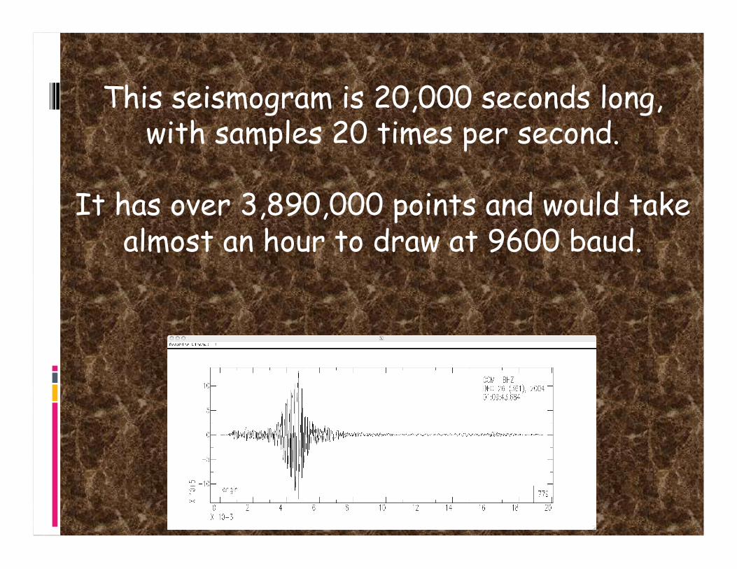
This seismogram is 20,000 seconds long, with samples 20 times per second.

It has over 3,890,000 points and would take almost an hour to draw at 9600 baud.

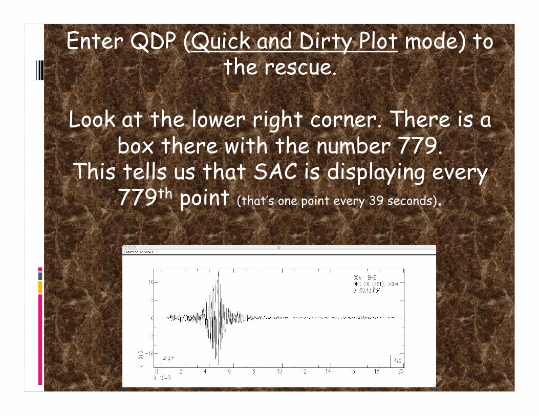
Enter QDP (Quick and Dirty Plot mode) to the rescue.

Look at the lower right corner. There is a box there with the number 779.

This tells us that SAC is displaying every 779th point (that’s one point every 39 seconds).

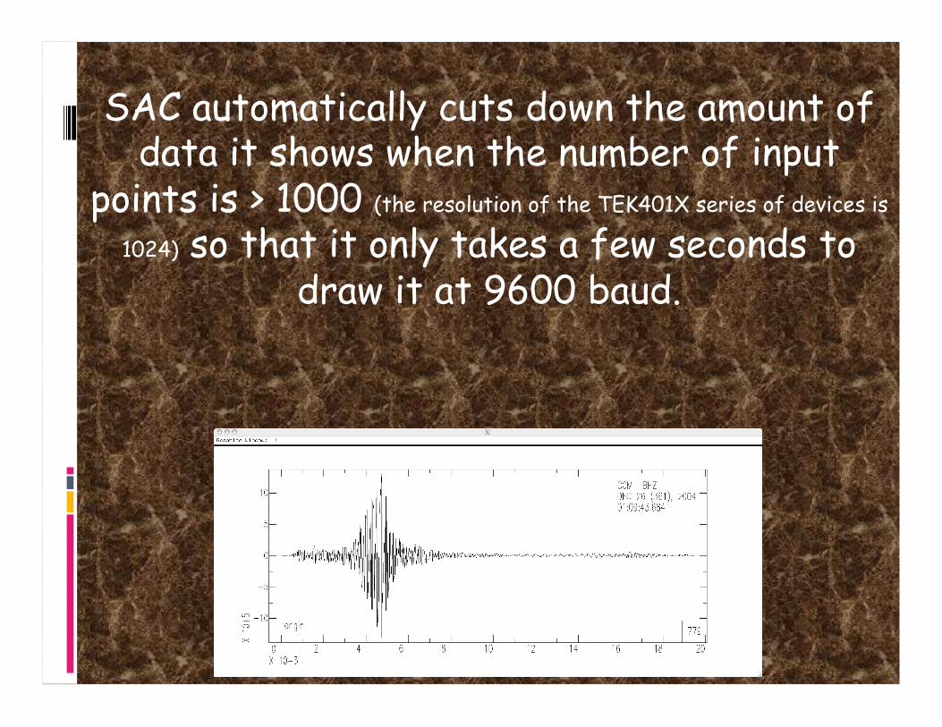
SAC automatically cuts down the amount of data it shows when the number of input

points is > 1000 (the resolution of the TEK401X series of devices is

1024) so that it only takes a few seconds to draw it at 9600 baud.

Unfortunately, about the only thing this plot tells us is that something was recorded.

The wiggles you see are completely useless for analysis

(you will learn the technical reasons for this in signal analysis).

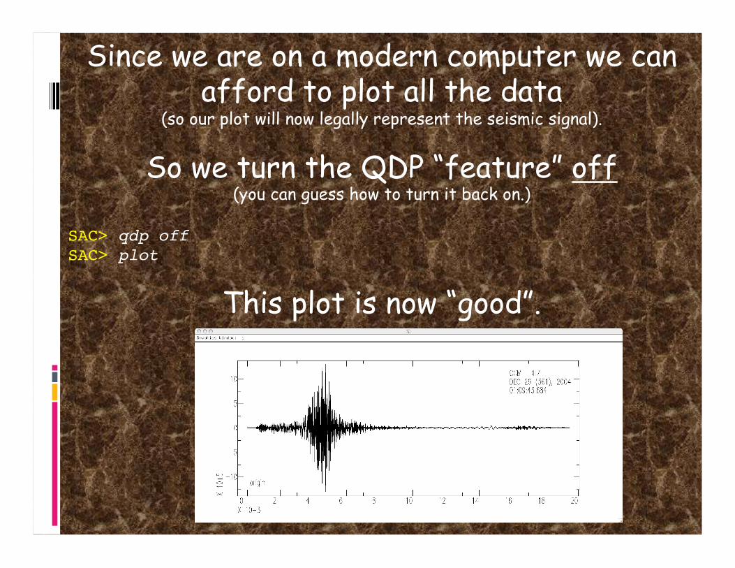
Since we are on a modern computer we can afford to plot all the data

(so our plot will now legally represent the seismic signal).

So we turn the QDP “feature” off (you can guess how to turn it back on.)

SAC> qdp off SAC> plot

This plot is now “good”.

qdp is the correct idea (don’t waste time displaying stuff that

you can’t see due to screen resolution), but it is badly implemented.

qdp should have taken the max and min of each of the sections of N points (instead of each Nth

point) and plotted a vertical line between them at each time (it would have taken twice as long to display, but the

display was relatively quick).

The display would be identical to the full display on the last slide (and look like a paper record).

(this would have cost some computer time, but that is minimal compared to the data transfer time to the TEK401X).

So far there is one file in memory.

If we simply read in another one – it will clobber what we have there.

If we need to read in more data (say we have processed the data we’ve read in and now

want a spectral ratio of the processed data with the original data) we have to use the

“more” option to read in the additional data.

read more filename

In general SAC does commands to all the files in memory.

If the command is starting from scratch (like a read) it clobbers what is already

there.

Some commands require certain pairs of files

(N and E for example for rotating seismograms).

We have now seen 4 SAC commands (but only used 3).

read filename write still to be determined

plot qdp on or off

Unfortunately SAC does not allow you to move around through the command line or

“history” with the cursor keys (was not part of the PRIMEOS).

You have to retype stuff (although you can use the GUI to highlight text and copy and paste it).

Let’s try a few more things.

Here I have to be a little more careful when I specify the file name. I want to read in all

3 components of the seismogram.

(I’ve also demonstrated the feature of SAC, that if it does not understand a command, it passes it to the OS for further processing.

Based on the output of the “ls” command, I don’t want SAC to read in the “.ai”, “.ps”, or “.tif” format files – although if I try to read them SAC will generate an

error message that it cannot understand them and just skip/ignore them).

SAC> ls *sumatra*bh* ccm_sumatra_.bhe ccm_sumatra_.bhn ccm_sumatra_.bhz ccm_sumatra_bhz.ai ccm_sumatra_bhz.ps ccm_sumatra_bhz.tif SAC> r *sumatra*bh? ccm_sumatra_.bhe ccm_sumatra_.bhn ccm_sumatra_.bhz

Try the plot command. SAC> plot Waiting

SAC plots the traces one at a time, in the order they are stored in memory (these happen to be

in alphabetical order – BHE, BHN and BHZ – due to the wildcard expansion). Each time you enter a <CR> it plots the next

trace. (and says Waiting if there are more traces to display, or the prompt if not).

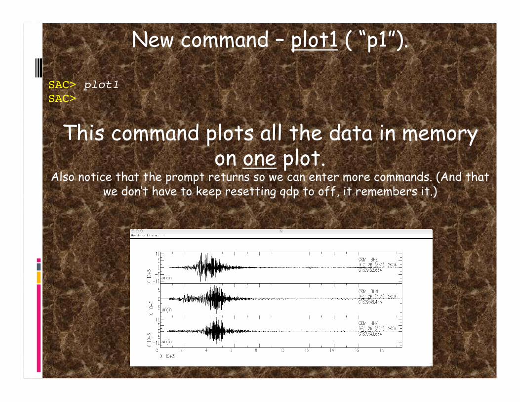
New command – plot1 ( “p1”).

SAC> plot1 SAC>

This command plots all the data in memory on one plot.

Also notice that the prompt returns so we can enter more commands. (And that we don’t have to keep resetting qdp to off, it remembers it.)

Say I want to process these three traces together.

UGLY little detail.

Notice that the three traces do not start at the same time (and we will see that they are

not the same lengths, either).

We can fix the time alignment using

synchronize (“synch”): which modifies (the

headers of) the files in memory so that they all have the same reference time.

(Does not otherwise modify the data. If I need to combine two traces and they are not the same length, SAC will complain and not do it.)

SAC> synch SAC> plot1

How do we find out what do we have in memory?

What metadata is available about the seismic data?

(metadata is data about data – examples are the name of the seismic station and component, the sampling rate, etc. This information is stored in the SAC

header.)

listhdr (lh): lists the headers of the files in memory.

SAC> listhdr FILE: ccm_sumatra_.bhe - 1 ---------------------- NPTS = 389396 B = 0.000000e+00 E = 1.946975e+04 IFTYPE = TIME SERIES FILE LEVEN = TRUE DELTA = 5.000000e-02 IDEP = UNKNOWN DEPMIN = -1.073057e+06 DEPMAX = 1.091875e+06 DEPMEN = 8.429739e+02 OMARKER = 7.315 (origin ) KZDATE = DEC 26 (361), 2004 KZTIME = 01:09:52.684 IZTYPE = BEGIN TIME KSTNM = CCM CMPAZ = 9.000000e+01 CMPINC = 9.000000e+01 STLO = -9.124470e+01 DIST = 8.818225e+03 AZ = 1.854116e+02 BAZ = 2.013326e+02 LOVROK = TRUE NVHDR = 6 LPSPOL = TRUE LCALDA = TRUE KCMPNM = BHE KNETWK = US

All sorts of good stuff. Look in SAC

documentation for full details.

Obvious/important –

File name - FILE Number points – NPTS Beginning time offset - B Sampling rate – DELTA Start date – KZDATE Start time –KZTIME Station – KSTN Orientation – CMPAZ

May have info about stn location, event locn, … .

Says Waiting when page is full (may not be complete header listing).

<CR> to continue till run out of stuff to display.

(there is no way to “break” out of the commands (e.g.: plot, listhdr, …) that do

something for each file. You have to <CR> till it finishes.)

FILE: ccm_sumatra_.bhe – 1 NPTS = 389396 B = 0.000000e+00 KZDATE = DEC 26 (361), 2004 KZTIME = 01:09:52.684 FILE: ccm_sumatra_.bhn – 2 NPTS = 389328 B = 0.000000e+00 KZDATE = DEC 26 (361), 2004 KZTIME = 01:09:48.485 FILE: ccm_sumatra_.bhz – 3 NPTS = 389600 B = 0.000000e+00 KZDATE = DEC 26 (361), 2004 KZTIME = 01:09:43.684

B = 0.000000e+00 KZDATE = DEC 26 (361), 2004 KZTIME = 01:09:52.684

B = -4.199000e+00 KZDATE = DEC 26 (361), 2004 KZTIME = 01:09:52.684

B = -9.000000e+00 KZDATE = DEC 26 (361), 2004 KZTIME = 01:09:52.684

Before synch After synch

To make them all the same length

- Read them, then synch them (this gets them all aligned on the same relative 0 – the time of the latest file)

- Write them out (this clobbers the original),

- Set up a cut (which reads from a start to end time with respect to

reference time [ which we aligned above], not number of samples) and

- Read them again (under control of the cut).

- (Write out again (if you want to save them, clobbering what was

there). (I don’t know how to do this “in-place”, you need the write and re-read since the

SAC commands do not modify the files in memory.)

SAC> w over SAC> cut 0 8000 SAC> r ccm_sumatra_.bhe ccm_sumatra_.bhn ccm_sumatra_.bhz SAC> p1

And they all have the following in their header

NPTS = 160001 B = 0.000000e+00 E = 8.000000e+03 KZDATE = DEC 26 (361), 2004 KZTIME = 01:09:52.684

cut: defines how much of a data file is to be read.

You need to re-read the data after specifying a cut. (specifying the cut does not effect data in

memory)

You can also specify the cut with respect to times stored in the header (p wave arrival time for example) 5 s before, 30 s after t1

pick

SAC> cut t1 -5 30 SAC> r

Commands to see/change header values

listhdr (lh): list the header contents.

readhdr (rh) and writehdr (wh): read and write headers without the data.

chnhdr (ch): change header values.

copyhdr : copy header values from one file to the others in memory.

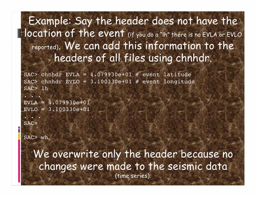
Example: Say the header does not have the location of the event (if you do a “lh” there is no EVLA or EVLO

reported). We can add this information to the headers of all files using chnhdr.

SAC> chnhdr EVLA = 4.079930e+01 # event latitude SAC> chnhdr EVLO = 3.100330e+01 # event longitude SAC> lh . . . EVLA = 4.079930e+01 EVLO = 3.100330e+01 . . . SAC>

SAC> wh

We overwrite only the header because no changes were made to the seismic data

(time series).

When you download preprocessed seismic data from the IRIS-DMC associated with an earthquake it will now have the earthquake location, origin time, delta, azimuth, etc. in

the header.

If you download data in some arbitrary time window (even if it has a big earthquake in it) it will not come with information about anything in particular within that time window (may be multiple events or none!).

You will have to put in the event information (SAC now computes the delta and az/baz and stores it in the header for you).

Graphics Action Module

REVIEW

plot (p): plots each signal in memory on a separate plot.

plot1 (p1): plots a set of signals on a single plot with a common x axis and separate y

axes.

NEW

plot2 (p2): plots set of signals on a single plot with common x and y axes (i.e. an overlay plot).

SAC> p1

SAC> p1 rel

Can plot each file relative to its begin time. (default is absolute, so the traces are shifted by actual time)

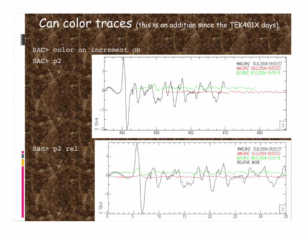
SAC> color on increment on

SAC> p2

Sac> p2 rel

Can color traces (this is an addition since the TEK401X days).

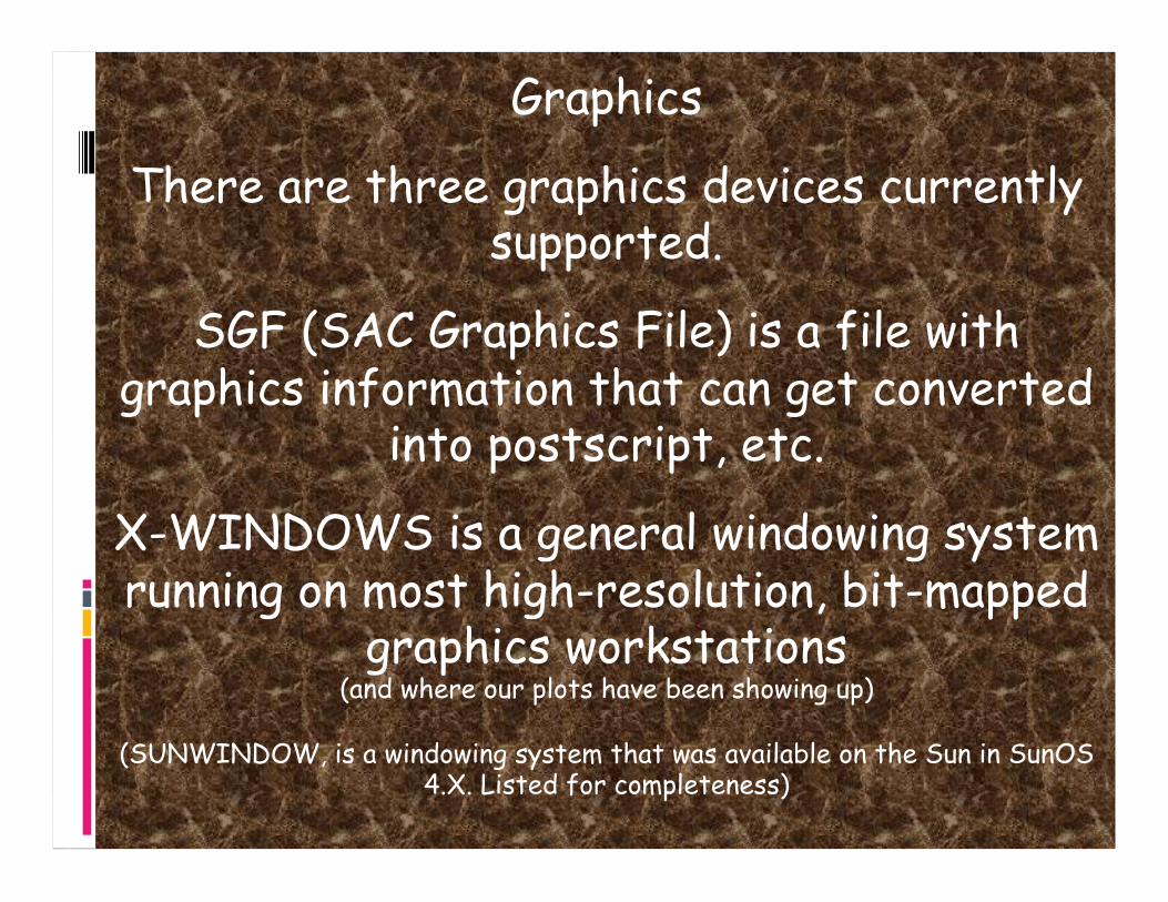
Graphics

There are three graphics devices currently supported.

SGF (SAC Graphics File) is a file with graphics information that can get converted

into postscript, etc.

X-WINDOWS is a general windowing system running on most high-resolution, bit-mapped

graphics workstations (and where our plots have been showing up)

(SUNWINDOW, is a windowing system that was available on the Sun in SunOS 4.X. Listed for completeness)

X-windows or X

X is widely used on UNIX graphics workstations and offers one of the best

frameworks (UNIX opinion, X follows the UNIX philosophy so it is

powerful and difficult) for developing portable window-based applications.

It should be the default graphics device when you start SAC.

Can be turned on using begin device: (bg).

sac> bd x

SGF demonstrates the power (or kluginess) of SAC and UNIX.

Rather than burden the SAC program with producing graphics for a large number of

possible devices (postscript did not even exist when SAC was written)

have SAC write out a file (that is probably just the

TEK401X commands) that some other programs read and translate into the appropriate format

for display on any particular device.

SAC Graphics Files contain all the information needed to generate a single plot.

Each plot is stored in a separate file.

The file names are of the form “fnnn.sgf” where nnn is the plot number, beginning with

001, each time you start SAC (so if you have some preexisting files they will get clobbered – you have been

forewarned).

SGF output is turned on with the command begindevice: (bg)

sac> bd sgf

Graphics output will now go to the sgf file.

You will not see it on the screen (X display).

There is no “save my figure” from the X-display

(this is UNIX and without an inordinate amount of work to bring out its power, X is very basic).

So if you want to make a figure for printing or sending anywhere but the X-display

(if it is a complicated figure you may have to first make it and look at it on the X-display -

then).

Turn on the sgf device and (RE)make it with the output now going to the file.

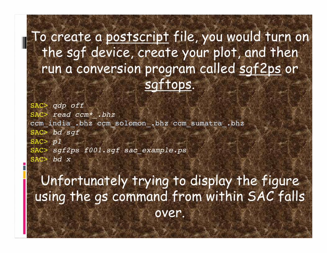
To create a postscript file, you would turn on the sgf device, create your plot, and then run a conversion program called sgf2ps or

sgftops. SAC> qdp off SAC> read ccm*_.bhz ccm_india_.bhz ccm_solomon_.bhz ccm_sumatra_.bhz SAC> bd sgf SAC> p1 SAC> sgf2ps f001.sgf sac_example.ps SAC> bd x

Unfortunately trying to display the figure using the gs command from within SAC falls

over.

Data Format and Header

Each signal or seismogram is stored in a separate binary or alphanumeric data file.

SAC can read data in a variety of formats: - SAC Binary Format (most common)

- SAC ASCII Format - CSS format - SDD format

- ASCII formats

Each data file contains a header (we have already seen

a bit about the header) that describes the contents of that file.

Some header fields

Time

The SAC header contains a reference or zero time, stored as six integers (NZYEAR, NZJDAY,

NZHOUR, NZMIN, NZSEC, NZMSEC), but normally printed in an equivalent alphanumeric format (KZDATE and

KZTIME), the offset in seconds between the reference and the data start time (B) and the number of seconds to the data end time (E).

B = 0.000000e+00 E = 3.600990e+03 KZDATE = APR 06 (097), 2008 KZTIME = 02:59:59.320

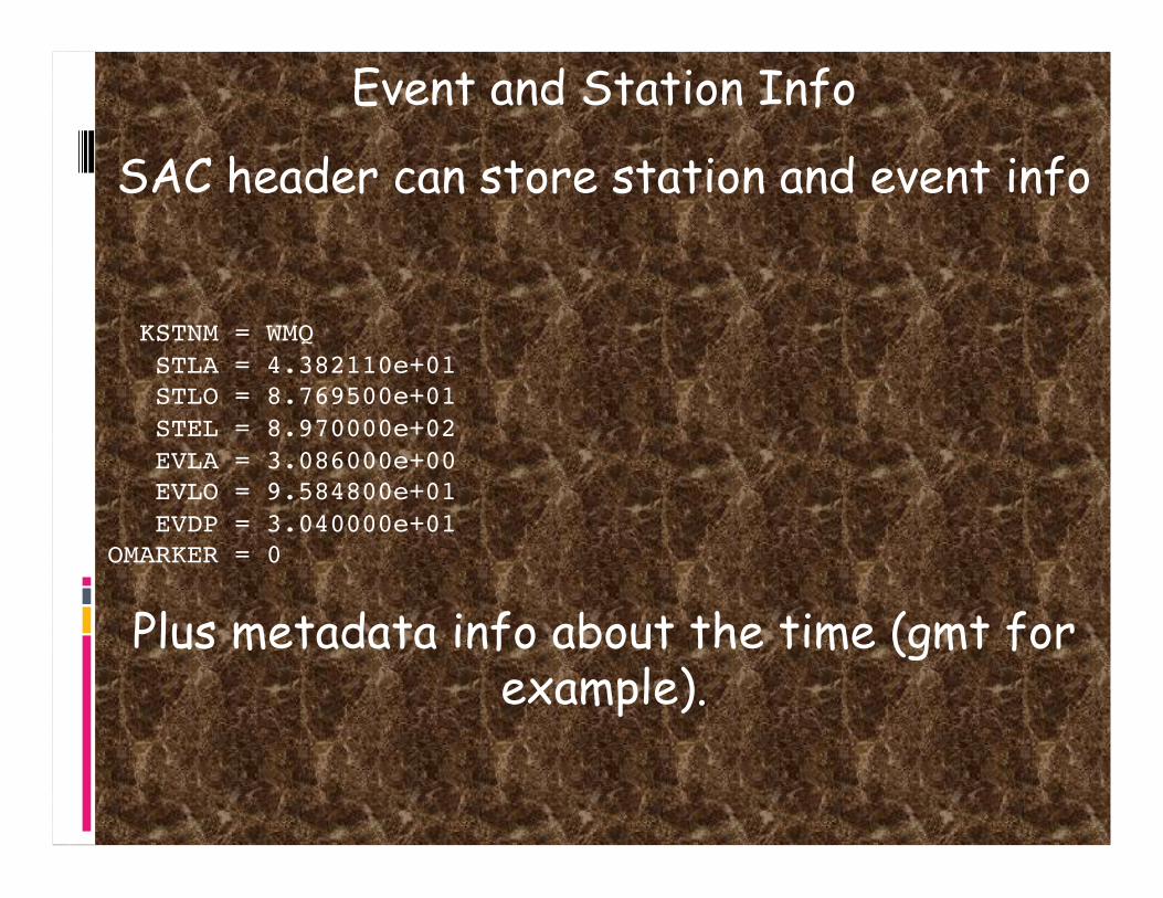
Event and Station Info

SAC header can store station and event info

KSTNM = WMQ STLA = 4.382110e+01 STLO = 8.769500e+01 STEL = 8.970000e+02 EVLA = 3.086000e+00 EVLO = 9.584800e+01 EVDP = 3.040000e+01 OMARKER = 0

Plus metadata info about the time (gmt for example).

If the event and station information are in the header, SAC automatically calculates and

stores

distance (in km) azimuth (in degrees)

backazimuth (in degrees) and great circle arc length (in degrees)

in the header (SAC2000 and later, earlier versions did not do this).

DIST = 4.583862e+03 AZ = 3.510350e+02 BAZ = 1.675856e+02 GCARC = 4.120298e+01

Phase Info

SAC can be used to pick and store phase information in header variables A & T0-T9 (although this is another place where it shows its age and is quite clumsy).

Omarker is reserved to for the origin time.

All pick and origin times are stored in seconds from the reference time of the file.

omarker (origin time) is oftentimes set (incorrectly) to zero.

If amarker and t0marker are not set, they will not show in a lh.

OMARKER = 0 AMARKER T0MARKER T1MARKER = 462.7 (P) T2MARKER = 834.76 (S) T4MARKER = 472.5 (pP) T6MARKER = 478 (sP)

You can also store what you think the time is.

Filtering and Spectral Analysis

funcgen: generate various functions in memory.

STEP BOXCAR TRIANGLE SINE {v1 v2} LINE {v1 v2} IMPULSE QUADRATIC {v1 v2 v3} CUBIC {v1 v2 v3 v4} SEISMOGRAM DATAGEN RANDOM {v1 v2} IMPSTRIN {n1 n2 ... nN}

It is VERY useful for testing the other commands on known functions.

(seismogram is obsolete, replaced by datagen, but datagen reports missing the directory with the sample files. Typical!) (Chuck still has old version installed.)

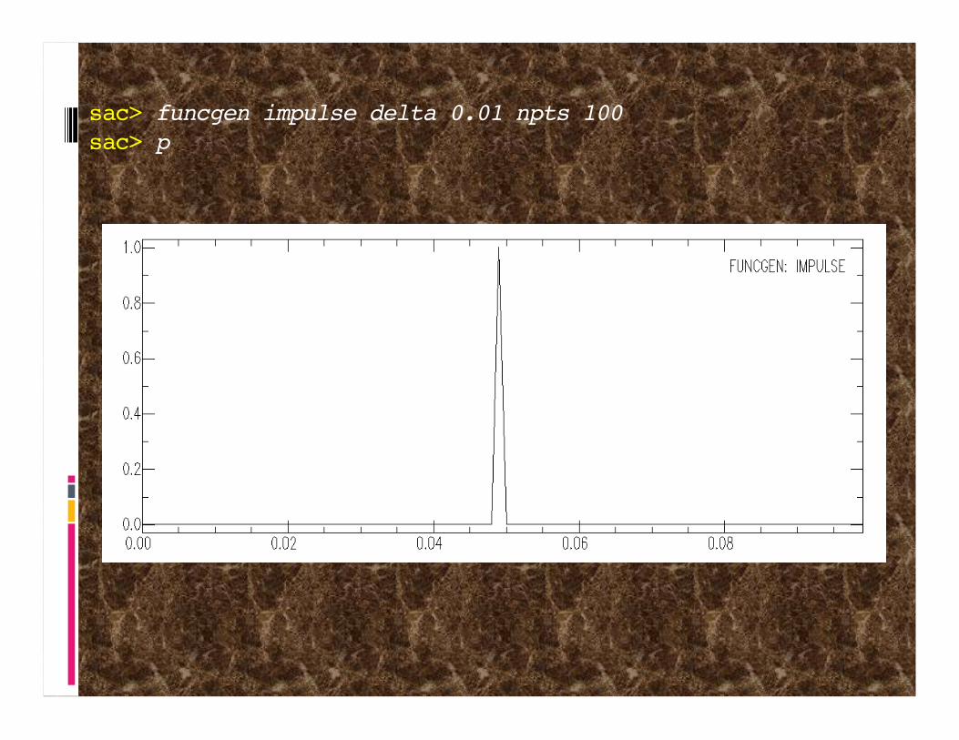
sac> funcgen impulse delta 0.01 npts 100sac> p

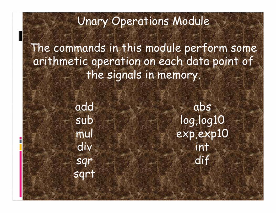
Unary Operations Module

The commands in this module perform some arithmetic operation on each data point of

the signals in memory.

add sub mul div sqr sqrt

abs log,log10

exp,exp10 int dif

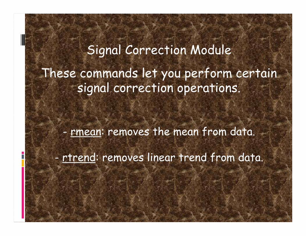
Signal Correction Module

These commands let you perform certain signal correction operations.

-  rmean: removes the mean from data.

-  rtrend: removes linear trend from data.

- rglitches: removes glitches and timing marks.

-  taper: applies a symmetric taper to each end of the data and SMOOTH applies an arithmetic

smoothing algorithm.

-  linefit: computes the best straight line fit to the data in memory and writes the results to header

blackboard variables.

- reverse: reverses the order of data points.

Integration – to change from acceleration to velocity to displacement.

SAC> r ccm_india_.bhz SAC> qdp off SAC> plot

Integrate it (original data was vel, integrate to disp).

SAC> int SAC> p

OOPS!

What is the problem?

(do you agree that there is a problem!)

Integral of constant is a line. Seismic data has DC offset. So remove mean.

SAC> r SAC> rmean SAC> int SAC> p

OOPS again!

Is this an improvement? Are we getting any better?

What’s the problem now?

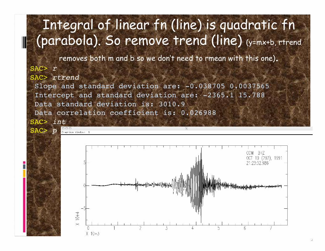
Integral of linear fn (line) is quadratic fn (parabola). So remove trend (line) (y=mx+b, rtrend

removes both m and b so we don’t need to rmean with this one). SAC> r SAC> rtrend Slope and standard deviation are: -0.038705 0.0037565 Intercept and standard deviation are: -2365.1 15.788 Data standard deviation is: 3010.9 Data correlation coefficient is: 0.026988 SAC> int SAC> p

There is still some “drift”, but this is probably useful for displacement analysis.

SAC> r SAC> rtrend Slope and standard deviation are: -0.038705 0.0037565 Intercept and standard deviation are: -2365.1 15.788 Data standard deviation is: 3010.9 Data correlation coefficient is: 0.026988 SAC> int SAC> r more SAC> p1

SAC> r more SAC> p1 displacement

velocity

Differentiation - default is 2 point difference y=(x1-x0)/delta. sac> funcgen impulse delta 0.01 npts 100sac> dif sac> p

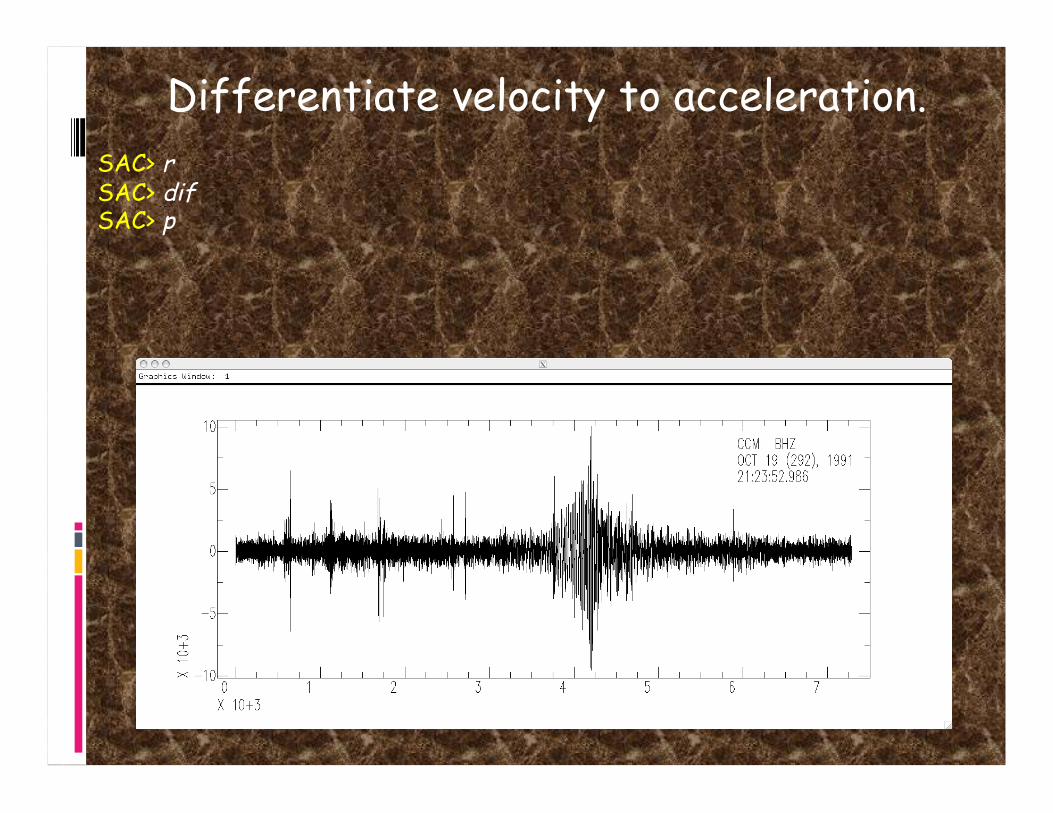
Differentiate velocity to acceleration. SAC> r SAC> dif SAC> p

Binary Operations Module

These commands perform operations on pairs of data files.

-  merge: merges (concatenates) a set of files to the data in memory.

-  addf: adds a set of data files to the data in memory.

-  subf: subtracts a set of data files from the ones in memory.

-  mulf: multiplies a set of data files by the data in memory.

-  divf: divides the data in memory by a set of files.

- binoperr: controls errors that can occur during these binary operations.

sac> funcgen impulse delta 0.01 npts 100sac> w impulse1.sacsac> div 2 sac> w impulse2.sacsac> r impulse1.sacsac> addf impulse2.sac

Notice you have to write intermediate stuff out to disk.

sac> funcgen sine 10 90 delta 0.01 npts 100sac> p

sac> taper

More

-  stretch: upsamples data, including an optional interpolating FIR filter.

-  decimate: downsamples data, including an optional anti-aliasing FIR filter.

- interpolate: interpolate evenly or unevenly spaced data to a new sampling interval using the

interpolate command.

More -  quantize: converts continuous data into its

quantized equivalent.

-  rotate: pairs of data components through a specified angle.

- rq: removes the seismic Q factor from spectral data.

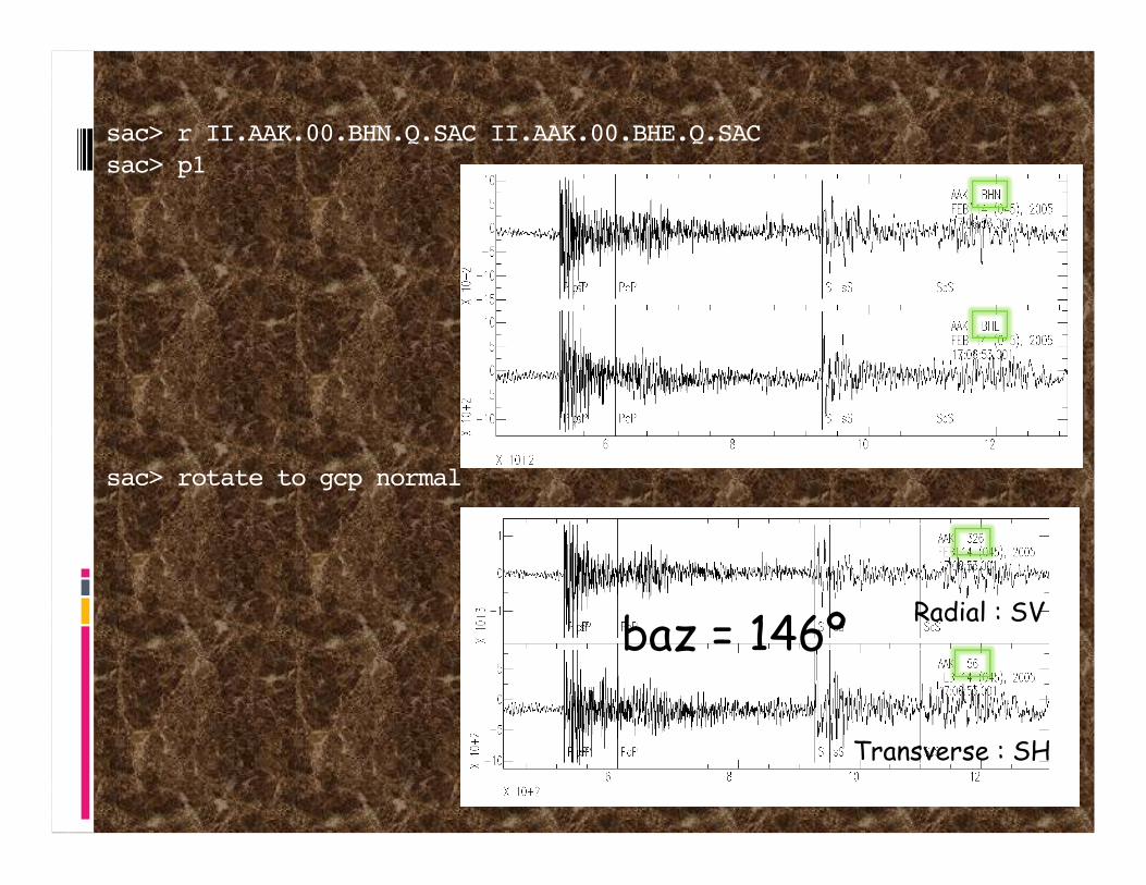
sac> r II.AAK.00.BHN.Q.SAC II.AAK.00.BHE.Q.SACsac> p1

sac> rotate to gcp normal

Radial : SV

Transverse : SH

baz = 146º

Spectral Analysis Module

There is a set of Infinite Impulse Response (IIR) filters.

-  lowpass: (lp) passes signal below a high corner cutoff.

- highpass: (hp) passes signal above a low corner cutoff).

- bandpass: (bp) pass signal within the low and high corner cutoffs.

-  bandrej: (br) band reject filter does the opposite of a bandpass.

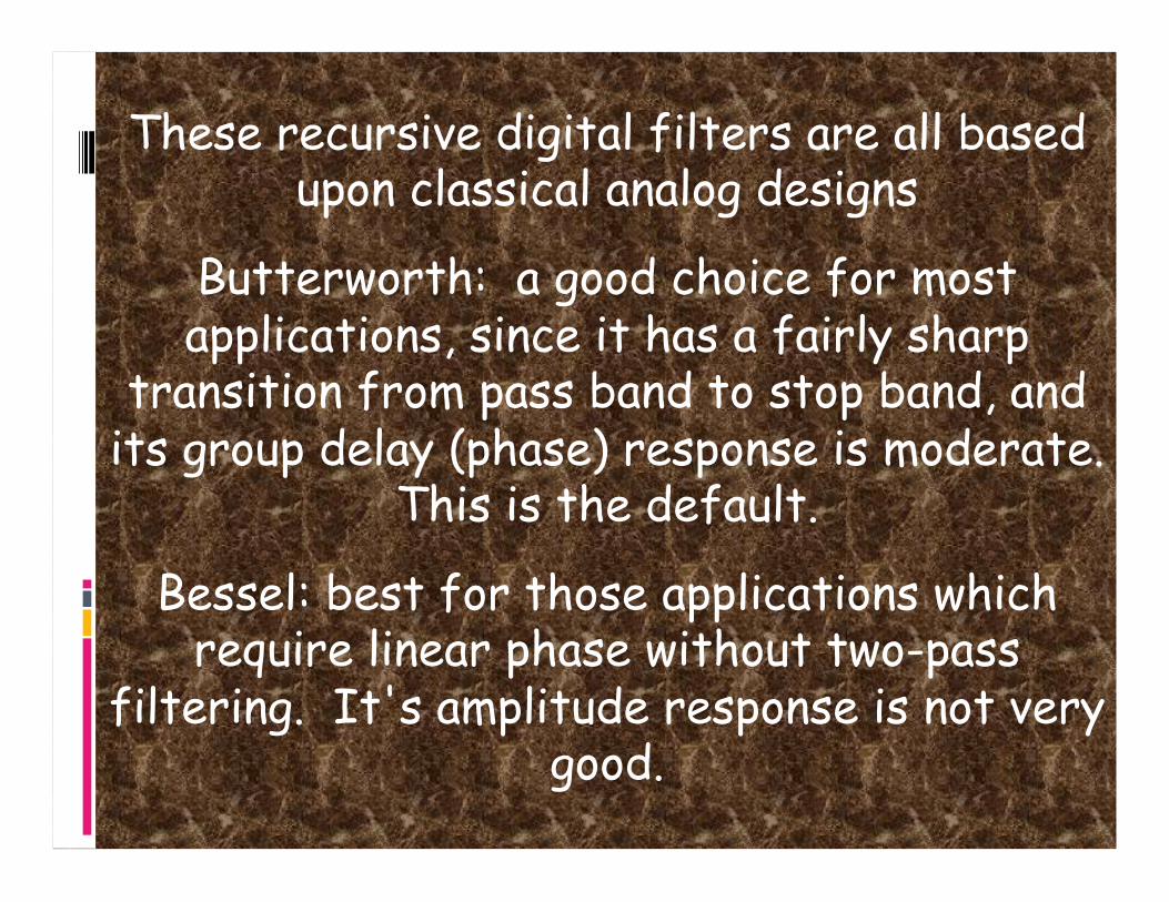
These recursive digital filters are all based upon classical analog designs

Butterworth: a good choice for most applications, since it has a fairly sharp

transition from pass band to stop band, and its group delay (phase) response is moderate.

This is the default.

Bessel: best for those applications which require linear phase without two-pass

filtering. It's amplitude response is not very good.

Chebyshev type I & Chebyshev type II: for situations which require very rapid

transitions from pass band to stop band. Does horrible things to the phase.

The Butterworth and Bessel are the easiest to set up BANDPASS {BUTTER|BESSEL|C1|C2},{CORNERS v1 v2},{NPOLES n},{PASSES n},{TRANBW v},{ATTEN v}

sac> funcgen seismogram

sac> rmeansac> tapersac> bp butter co 1 3

using default values passes (p) 1 num poles (n) 2

sac> hp butter co .2sac> xlim t1 -120 800

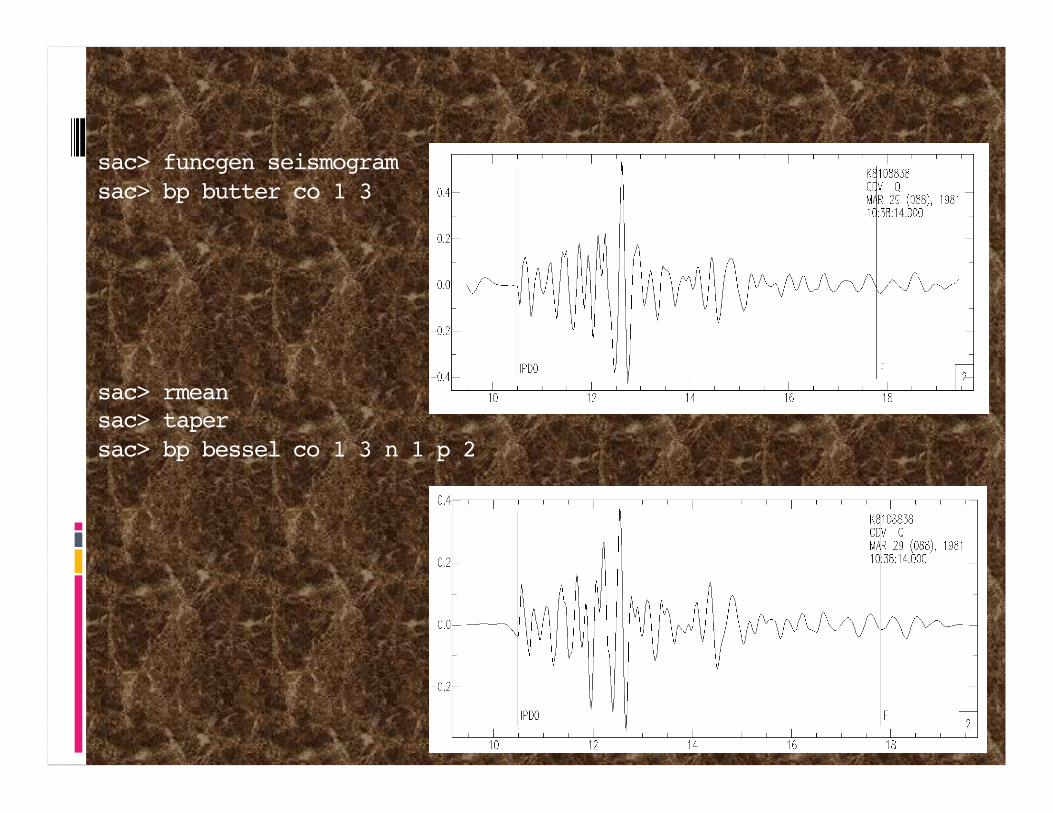
sac> funcgen seismogramsac> bp butter co 1 3

sac> rmeansac> tapersac> bp bessel co 1 3 n 1 p 2

Other filters

Finite Impulse Response filter (FIR).

Adaptive Wiener filter. (It tailors itself to be the “best possible filter” for a given dataset.).

Two specialized filters (BENIOFF & KHRONHITE).

(lowpass filter is a digital approximation of an analog filter which was a cascade of two fourth-order Butterworth lowpass filters. This lowpass filter has been

used with a corner frequency of 0.1 Hz to enhance measurements of the amplitudes of the fundamental mode Rayleigh wave (Rg) at regional distances.)

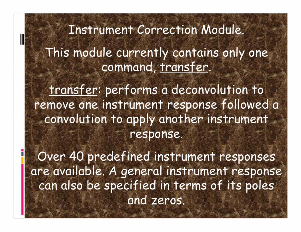
Instrument Correction Module.

This module currently contains only one command, transfer.

transfer: performs a deconvolution to remove one instrument response followed a

convolution to apply another instrument response.

Over 40 predefined instrument responses are available. A general instrument response

can also be specified in terms of its poles and zeros.

sac> funcgen seismogramsac> transfer to wa

Usually you would remove the known instrument response using ‘transfer from

XXX’.

Why would you want to remove the instrument response and apply the response for a Wood-Anderson torsion seismometer?

Let’s say you’ve downloaded some data from IRIS, unpacked the seed volume using rdseed,

and extracted the response files. (RESP.NET.STA.LOC.CHAN)

transfer can read seed response files (evalresp) and transforms velocity to displacement (none).

sac> r BJT*sac> rtrend sac> rmean sac> transfer from evalresp to none

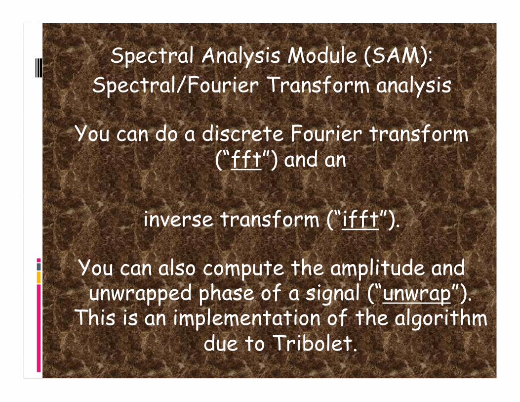
Spectral Analysis Module (SAM): Spectral/Fourier Transform analysis

You can do a discrete Fourier transform (“fft”) and an

inverse transform (“ifft”).

You can also compute the amplitude and unwrapped phase of a signal (“unwrap”).

This is an implementation of the algorithm due to Tribolet.

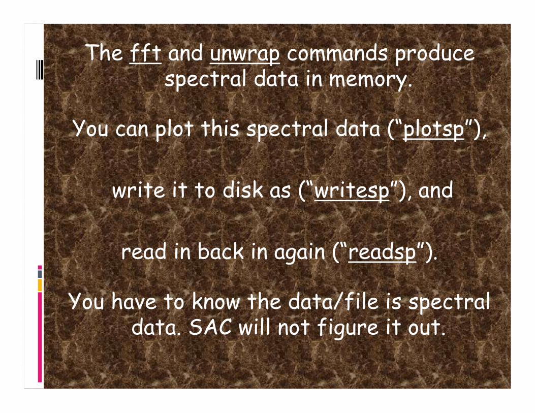
The fft and unwrap commands produce spectral data in memory.

You can plot this spectral data (“plotsp”),

write it to disk as (“writesp”), and

read in back in again (“readsp”).

You have to know the data/file is spectral data. SAC will not figure it out.

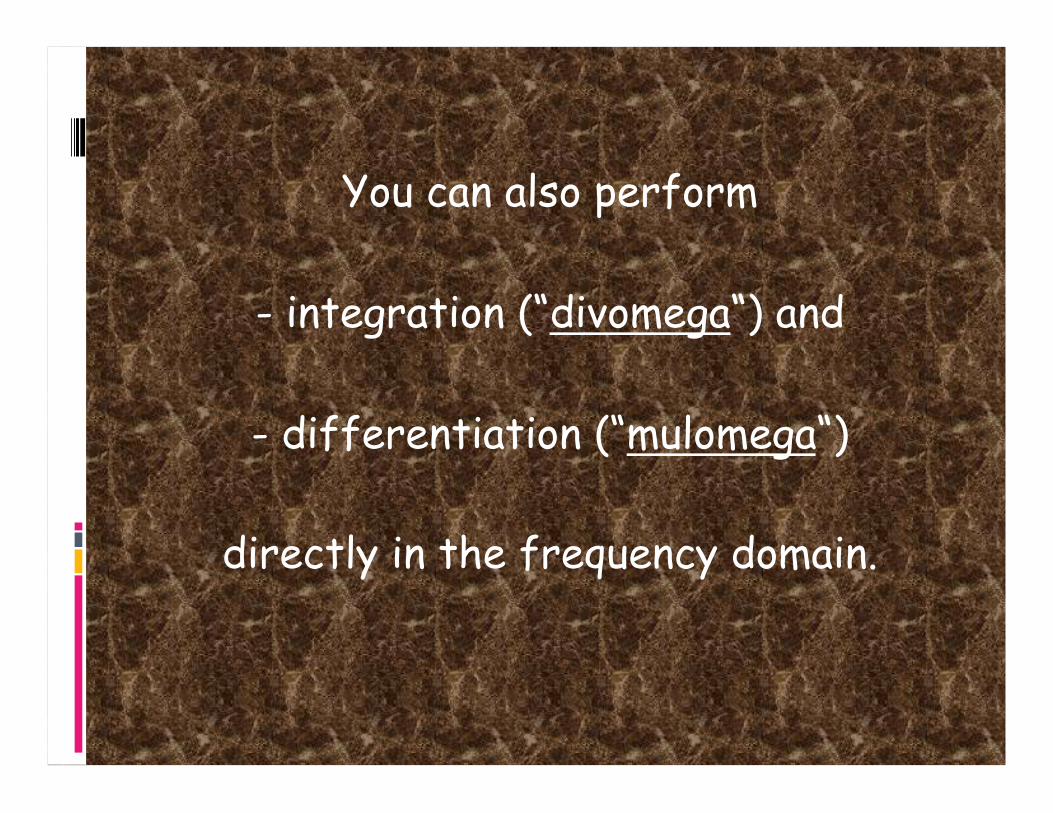
You can also perform

- integration (“divomega“) and

- differentiation (“mulomega“)

directly in the frequency domain.

sac> funcgen seismogram sac> fft sac> plotsp

amplitude

phase

SPECTROGRAM (DEFAULT VALUES: SPECTROGRAM WINDOW 2, SLICE 1, METHOD MEM,

ORDER 100, NOSCALING, YMIN 0, YMAX FNYQUIST, COLOR)

sac> funcgen seismogramsac> spectrogram ymin 0 ymax 20Window size: 200 Overlap: 100 FFT size: 512 Spectrogram dimensions are 512 by 9 .

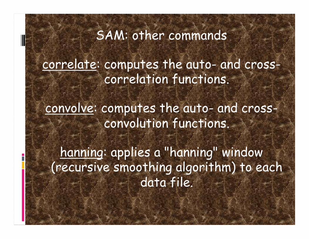
SAM: other commands

correlate: computes the auto- and cross-correlation functions.

convolve: computes the auto- and cross-convolution functions.

hanning: applies a "hanning" window (recursive smoothing algorithm) to each

data file.

SAM: other commands

hilbert: applies a Hilbert transform (90º phase shift at all frequencies in the

signal). Applied twice, this flips the sign of the amplitude.

envelope: computes the envelope function using a Hilbert transform.

sac> funcgen seismogramsac> w seism.sacsac> tapersac> envelopesac> w envelope.sacsac> r seism.sac envelope.sacsac> color on increment onsac> p2