basic crystallography part 1 - university of...
TRANSCRIPT

Basic Crystallography Part 1
Theory and Practice of X-ray
Crystal Structure Determination

Course Overview
Basic Crystallography – Part 1 n Introduction: Crystals and Crystallography n Crystal Lattices and Unit Cells n Generation and Properties of X-rays n Bragg's Law and Reciprocal Space n X-ray Diffraction Patterns from Crystals
Basic Crystallography – Part 2 n Review of Part 1 n Selection and Mounting of Samples n Unit Cell Determination n Intensity Data Collection n Data Reduction n Structure Solution and Refinement n Analysis and Interpretation of Results

Introduction to Crystallography

What are Crystals?
4

Examples of Crystals

Examples of Protein Crystals

Growing Crystals
Kirsten Böttcher and Thomas Pape

We have a crystal…
… we want a structure!
How do we get there ?

Crystal Systems and Crystal Lattices

Foundations of Crystallography
n Crystallography is the study of crystals.
n Scientists who specialize in the study of crystals are called crystallographers.
n Early studies of crystals were carried out by mineralogists who studied the symmetries and shapes (morphology) of naturally-occurring mineral specimens.
n This led to the correct idea that crystals are regular three-dimensional arrays (Bravais lattices) of atoms and molecules; a single unit cell is repeated indefinitely along three principal directions that are not necessarily perpendicular.

What are Crystals?
11
n A crystal or crystalline solid is a solid material whose constituent atoms, molecules, or ions are arranged in an orderly, repeating pattern extending in all three spatial dimensions.

The Unit Cell Concept
Ralph Krätzner

a
b
c
αβ
γ
Unit Cell Description in terms of Lattice Parameters
n a ,b, and c define the edge lengths and are referred to as the crystallographic axes.
n α, β, and γ give the angles between these axes.
n Lattice parameters à dimensions of the unit cell.

A
A crystal is… a homogenous solid formed by a repeating, three-dimensional pattern of atoms.
A A A A A A A A A A A A A A A A
The unit cell is the repeating unit with dimensions of a, b, c and angles α, β and γ. A crystal can be described completely by translations of the unit cell along the unit cell axes.
A
a
b
A + a
A + a
A + b
A + a

Choice of the Unit Cell (sometimes confusing)

Choice of the Unit Cell
No symmetry - many possible unit cells. A primitive cell with angles close to 90º (C or D) is preferable.
C D
A
B
C
A
The conventional C-centered cell (C) has 90º angles, but one of the primitive cells (B) has two equal sides.
B

The shortest possible introduction to crystallography There are seven types of unit cells (crystal systems).
Crystal systems: triclinic monoclinic orhorhombic tetragonal trigonal/hexagonal cubic
Bravais lattices: aP mP, mC oP, oA, oI, oF tP, tI hP, hR cP, cI, cF
P : primitive, A,B,C : face centered I : body centered F : (all-)face centered R : rhombohedral centered
α = γ = 90°
α = β = γ = 90°
α = β = γ = 90° a = b
α = β = γ = 90° a = b = c
α = β = 90° γ = 120°
a = b
Combined with centering, we obtain the 14 Bravais lattices.

The shortest possible introduction into crystallography
A A A A A A A A A A A A A A A A
The space group is the combination of Bravais lattice + symmetry of the crystal. Point group symmetry of a molecule does not necessarily imply that this symmetry is also present in the crystal.
A A A A A A A A A A A A A A A A
Independent values for both distances
Both distances are identical due to symmetry
Pm The unit cell contains:
two molecules one molecule

The shortest possible introduction into crystallography
A A A A A A A A A A A A A A A A
The asymmetric unit is the part of the unit cell, from which the rest of the unit cell is generated using symmetry operations. To build the complete crystal we need only the space group and the atom positions in the asymmetric unit.
A A A A A A A A A A A A A A A A
Independent values for both distances
Both distances are identical due to symmetry
Pm

7 Crystal Systems - Metric Constraints
n Triclinic - none
n Monoclinic - α = γ = 90°, β ≥ 90°
n Orthorhombic - α = β = γ = 90°
n Tetragonal - α = β = γ = 90°, a = b
n Cubic - α = β = γ = 90°, a = b = c
n Trigonal - α = β = 90°, γ = 120°, a = b (hexagonal setting) or α = β = γ , a = b = c (rhombohedral setting)
n Hexagonal - α = β = 90°, γ = 120°, a = b

Bravais Lattices
n Within each crystal system, different types of centering produce a total of 14 different lattices.
n P – Simple n I – Body-centered n F – Face-centered n B – Base-centered (A, B, or C-centered)
n All crystalline materials can have their crystal structure described by one of these Bravais lattices.

Bravais Lattices

Bravais Lattices

Crystal Families, Crystal Systems, and Lattice Systems

Example:
n The monoclinic space groups:
n P2 P21 C2 n Pm Pc Cm Cc n P2/m P21/m C2/m C2/c
2: two fold axis 21: screw axis or improper axis m: mirror plane c: sliding mirror or improper mirror

Crystal Families, Crystal Systems, and Lattice Systems

Generation of and Properties of X-rays

A New Kind of Rays
n Wilhelm Conrad Röntgen
n German physicist who produced and detected Röntgen rays, or X-rays, in 1895.
n He determined that these rays were invisible, traveled in a straight line, and affected photographic film like visible light, but they were much more penetrating.

Properties of X-Rays
n Electromagnetic radiation (λ = 0.01 nm – 10 nm)
n Wavelengths typical for XRD applications: 0.05 nm to 0.25 nm or 0.5 to 2.5 Å
1 nm = 10-9 meters = 10 Å
n E = ħc / λ

X-ray
Fast incident electron
nucleus
Atom of the anode material
electrons
Electron (slowed down and changed direction)
Generation of Bremsstrahlung Radiation
n “Braking” radiation. n Electron deceleration releases radiation across a spectrum of wavelengths.

Kα
Lα
Kβ
K
L
M
Emission Photoelectron
Electron
Generation of Characteristic Radiation
n Incoming electron knocks out an electron from the inner shell of an atom.
n Designation K,L,M correspond to shells with a different principal quantum number.

Bohr`s model
Generation of Characteristic Radiation
n Not every electron in each of these shells has the same energy. The shells must be further divided.
n K-shell vacancy can be filled by electrons from 2 orbitals in the L shell, for example.
n The electron transmission and the characteristic radiation emitted is given a further numerical subscript.

M
K
L
Kα1 Kα2 Kβ1 Kβ2
Energy levels (schematic) of the electrons
Intensity ratios Kα1 : Kα2 : Kβ = 100 : 50 : 20
Generation of Characteristic Radiation

Emission Spectrum of an X-Ray Tube

Emission Spectrum of an X-Ray Tube: Close-up of Kα
Cullity, B.D. and Stock, S.R., 2001, Elements of X-Ray Diffraction, 3rd Ed., Addison-Wesley

Sealed X-ray Tube Cross Section
n Sealed tube n Cathode / Anode
Cullity, B.D. and Stock, S.R., 2001, Elements of X-Ray Diffraction, 3rd Ed., Addison-Wesley
n Beryllium windows n Water cooled

Characteristic Radiation for Common X-ray Tube Anodes
Anode Kα1 (100%) Kα2 (50%) Kβ (20%)
Cu 1.54060 Å 1.54439 Å 1.39222 Å
Mo 0.70930 Å 0.71359 Å 0.63229 Å

Modern Sealed X-ray Tube
n Tube made from ceramic
n Beryllium window is visible.
n Anode type and focus type are labeled.

Sealed X-ray Tube Focus Types: Line and Point
Target
Line
Target
Filament Spot
Take-off angle n The X-ray beam’s cross section
at a small take-off angle can be a line shape or a spot, depending on the tube’s orientation.
n The take-off angle is the target-to-beam angle, and the best choice in terms of shape and intensity is usually ~6°.
n A focal spot size of 0.4 × 12 mm: 0.04 × 12 mm (line) 0.4 × 1.2 mm (spot)

Interaction of X-rays with Matter

d
wavelength λPr
intensity Io
incoherent scattering λCo (Compton-Scattering)
coherent scattering λPr (Bragg-scattering)
absorption Beer´s law I = I0*e-µd
fluorescence λ> λPr
photoelectrons
Interactions with Matter

Coherent Scattering
n Incoming X-rays are electromagnetic waves that exert a force on atomic electrons.
n The electrons will begin to oscillate at the same frequency and emit radiation in all directions.
e-

Interaction of X-rays with matter - Thomson-Diffusion -
e-
• The interaction with an electromagnetic field induces the oscillation of an electron
• Being an accelerated charged particle, the electron emits another electromagnetic wave.
hν hν

Constructive and Deconstructive Interference
0 100 200 300 400 500 600 700 800 900 1000
-1.4
-1.2
-1.0
-0.8
-0.6
-0.4
-0.2
0.0
0.2
0.4
0.6
0.8
1.0
Y Axis
Title
X Axis Title
0 100 200 300 400 500 600 700 800 900 1000
-1.4
-1.2
-1.0
-0.8
-0.6
-0.4
-0.2
0.0
0.2
0.4
0.6
0.8
1.0
Y Ax
is Ti
tle
X Axis Title
0 100 200 300 400 500 600 700 800 900 1000
-1.4
-1.2
-1.0
-0.8
-0.6
-0.4
-0.2
0.0
0.2
0.4
0.6
0.8
1.0
Y Axis T
itle
X Axis Title
0 100 200 300 400 500 600 700 800 900 1000
-1.4
-1.2
-1.0
-0.8
-0.6
-0.4
-0.2
0.0
0.2
0.4
0.6
0.8
1.0
Y Axis
Title
X Axis Title
0 100 200 300 400 500 600 700 800 900 1000
-1.4
-1.2
-1.0
-0.8
-0.6
-0.4
-0.2
0.0
0.2
0.4
0.6
0.8
1.0
Y Axis
Title
X Axis Title
=
=

θ2cos2422
4
crmeII iTh =
e-
For polarisation in y- direction:
The intensity of the diffracted X-ray beam depends on the diffusion angle.
y x
The image cannot be displayed. Your computer may not have enough memory to open the image, or the image may have been corrupted. Restart your computer, and then open the file again. If the red x still appears, you may have to delete the image and then insert it again.
The image cannot be displayed. Your computer may not have enough memory to open the image, or the image may have been corrupted. Restart your computer, and then open the file again. If the red x still appears, you may have to delete the image and then insert it again.
2θ
Interaction of X-rays with matter - Thomson-Diffusion -

Thomson diffusion
22cos1 2
422
4 θ+=
crmeII iTh
• The maximum intesity of the diffracted beam is less than 2%
Extension to non-polarised light yields:
• Polarisation factor P (later)
• ITh of neutrons is zero
• ITh (protons) = 10-7 ITh (electrons)
• I diminishes with distance
• Thomson diffusion is elastic: ωTh = ωi
• Thomson diffusion is coherent: ϕTh = ϕi + α (α = 180° pour e-)

Amorphous sample
Primary X-ray beam
X-ray experiment
Why do we need a single crystal ?
→ diffuse reflection

Crystalline sample Amorphous sample → diffuse reflection
X-ray experiment
Why do we need a single crystal ?
→ localised reflections

Polycrystalline sample Crystalline sample → localised reflections Amorphous sample → diffuse reflection
X-ray experiment
Why do we need a single crystal ?
→ overlapping reflections

Coherent Scattering by an Atom
n Coherent scattering by an atom is the sum of this scattering by all of the electrons.
n Electrons are at different positions in space, so coherent scattering from each generally has different phase relationships.
n At higher scattering angles, the sum of the coherent scattering is less.
2θ

Localised reflections - Laue construction Interactions of an X-ray beam with several diffracting centers
a·cos µ
a·cos ν
The intensity is only different from zero, when:
Δ = a·cos ν + a·cos µ = n·λ
a υ
µ

Why n·λ ?
I=0 Δ = ¼ λ
Δ = 1/3 λ
Δ = λ
I=0
I=I0

The Laue construction in 3 dimensions
a υ
µ
a·cos µ
a·cos ν
a·cos µa + a·cos νa = h·λ b·cos µb + b·cos νb = k·λ c·cos µc + c·cos νc = l·λ
3 equations, 6 angles, 3 distances ⇒ too complicated

Bragg construction
Glancing reflections at the lattice planes hkl of the crystal, which obey the Laue condition.
Bragg law:
2dhkl·sinθ = n·λ (n = 1, 2, 3 …)
θ θ
θ dhkl
d·sinθ
Thomson diffusion is coherent: ϕTh = ϕi + 180°

X-ray Diffraction by Crystals

Diffraction of X-rays by Crystals
n The science of X-ray crystallography originated in 1912 with the discovery by Max von Laue that crystals diffract X-rays.
n Von Laue was a German physicist who won the Nobel Prize in Physics in 1914 for his discovery of the diffraction of X-rays by crystals.
Max Theodor Felix von Laue (1879 – 1960)

X-ray Diffraction Pattern from a Single-crystal Sample
Rotation Photograph

Diffraction of X-rays by Crystals
After Von Laue's pioneering research, the field developed rapidly, most notably by physicists William Lawrence Bragg and his father William Henry Bragg.
In 1912-1913, the younger Bragg developed Bragg's law, which connects the observed scattering with reflections from evenly-spaced planes within the crystal.
William Lawrence Bragg
William Henry Bragg

Bragg’s Law
n X-rays scattering coherently from 2 of the parallel planes separated by a distance d.
n Incident angle and reflected (diffracted angle) are given by θ.

Bragg’s Law
n The condition for constructive interference is that the path difference leads to an integer number of wavelengths.
n Bragg condition à concerted constructive interference from periodically-arranged scatterers.
n This occurs ONLY for a very specific geometric condition.
θλ sin2
⋅= d θλ sin2dn =

Bragg’s Law
We can think of diffraction as reflection at sets of planes running through the crystal. Only at certain angles 2θ are the waves diffracted from different planes a whole number of wavelengths apart (i.e., in phase). At other angles, the waves reflected from different planes are out of phase and cancel one another out.
nλ = 2d sin(θ)
d θ θ

Reflection Indices
n These planes must intersect the cell edges rationally, otherwise the diffraction from the different unit cells would interfere destructively.
n We can index them by the number of times h, k and l that they cut each edge.
n The same h, k and l values are used to index the X-ray reflections from the planes.
z y
x
Planes 3 -1 2 (or -3 1 -2)
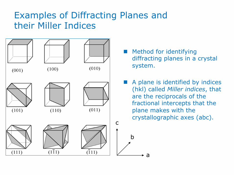
Examples of Diffracting Planes and their Miller Indices
a
b
c
n Method for identifying diffracting planes in a crystal system.
n A plane is identified by indices (hkl) called Miller indices, that are the reciprocals of the fractional intercepts that the plane makes with the crystallographic axes (abc).

Miller indices of lattice planes
a
b
a
b
110
• The plane nearest to the origin (not the plane through the origin), intersects the axes a, b and c at 1/h, 1/k and 1/l.
• An index of 0 indicates a plane parallel to an axis. • hkl are the “Miller indices” of the lattice planes • The higher the indices, the smaller the lattice spacing dhkl.
b = 1/k = 1 ð k = 1
a = 1/l = 1 ð l = 1

Miller indices of lattice planes
a
b
110
a
b
b = 1/k = 1 ð k = 1
a
b
a=1/2
b=1/1
210
a
b a=1/0 = ∞
b=1/3
a
b
a=1/-1
b=1/1
030
210
324 a
b
c
a = 1/l = 1 ð l = 1
a=1/3 b=1/2
c=1/4
x
x

What is 030 ?
030
a
b
There are no atoms in these planes. Why do we see reflections with them?

What is 030 ?
2d200 ·sinθ2 = λ, d200=d100/2 2d300 ·sinθ3 = λ, d300=d100/3 2dn00·sinθ = λ, dn00=d100/n
d100
θ1 θ1 θ2 θ2
2d100·sinθ2 = 2λ 2d100·sinθ3 = 3λ 2d100·sinθn = n·λ
2d100·sinθ1 = λ
d200
Thus, we have only first order reflections, but we have to add additional virtual hkl-planes.
n reflections for each plane 1 reflection for each plane, but additional planes

Diffraction Patterns
Two successive CCD detector images with a crystal rotation of one degree per image:
For each X-ray reflection (black dot), indices h,k,l can be assigned and an intensity I = F 2 measured

Reciprocal Space
n The immediate result of the X-ray diffraction experiment is a list of X-ray reflections hkl and their intensities I.
n We can arrange the reflections on a 3D grid based on their h, k and l values. The smallest repeat unit of this reciprocal lattice is known as the reciprocal unit cell; the lengths of the edges of this cell are inversely related to the dimensions of the real-space unit cell.
n This concept is known as reciprocal space; it emphasizes the inverse relationship between the diffracted intensities and real space.

From the position of primary and diffracted beam: → Orientation of the lattice planes in the crystal (perpendicular to the bisecting of the two beams)
Reflection angle θ : → Distance between lattice planes
Knowing the distances between lattice planes (dhkl) and their orientations, we obtain the unit cell.
180°-2θ
θ θ θ dhkl
X-ray experiment

Very fast: the reciprocal lattice
2
2
2
2
2
2
2
1cl
bk
ah
d++=
The distance d (dhkl) between lattice planes can be calculated from the unit cell parameters:
(orthorhombic system)
With the reciprocal values d* = 1/d, a* = 1/a, b* = 1/b, c* = 1/c we obtain:
2*22*22*22* clbkahd ++=
Each reflection hkl can thus be described as a vector d* = (h k l) in the reciprocal space formed by the basis vectors a*, b* and c*.
From the orientation of the primary and reflected beams, we obtain the direction of d* for each reflection, from the reflection angle theta the lattice spacing d and thus d* = 1/d. “Indexing” is the art to find a set of basis vectors a*, b*, c* which allow the description of each reflection with integer values of h, k and l.
• Finding the longest vectors which can describe all reflections
• A certain error must be allowed • If necessary, move to shorter basis vectors • From a*, b* and c*, the unit cell parameters and
the Miller indices are known.
020
220
110
100 200

Molecular structure: Atomic positions Crystalline structure:
Unit cell and space group
Crystal: Macroscopic dimensions
Crystallisation Single crystal selection
Structure determination
Dataset collection
Raw data
123 021
311
Détermination of the unit cell
Unit cell H K L I σ
0 0 1 134.4 12.5 0 0 2 0.2 1.2 1 1 4 52.4 2.2
Space group determination H K L I σ
0 0 1 134.4 12.5 0 0 2 0.2 1.2 1 1 4 52.4 2.2
Unit cell + space group: Dimensions and symmetry of
the crystalline structure Intensity of the reflections:
Atomic positions
Solution and Refinement

The seven crystal systems Which possibilities exist for a unit cell ?
Dimension Angle conditions conditions
Triclinic - -
Monoclinic - α = γ = 90o
Orthorhombic - α = β = γ = 90o
Tetragonal a = b α = β = γ = 90o
Trigonal, hexagonal a = b α = β = 90o, γ = 120o
Cubic a = b = c α = β = γ = 90o

The 14 Bravais lattices We obtain 14 Bravais lattices, when we combine the crystal systems with the centering. Centering describes that more than one “unit”/molecule is present in the unit cell (additional translational symmetry).
Primitive: P
Body centered: I
Face centered: A, B, C
a b
c
All-faces centered: F

Why do we need centered lattices ?
A A A
A A A
A A A
In the absence of symmetry, we can choose every possible unit cell.
If a C2 rotation axis or a mirror plane is present, only a monoclinc unit cell (or higher) is compatible with these symmetry elements. Without that symmetry it wouldn’t even be a monoclinic cell: it would be a triclinic cell with angles very, very close to 90o! To correctly describe our structure, we have always to choose the highest possible symmetry.

A A
A A A A
A
A
A A
A
A
A A A A A A A
A A A
A A
How can we describe a crystal which contains a certain symmetry, for example a C2 axis or a mirror plane, but the smallest cells are incompatible with these symmetry elements.
We choose a cell of higher volume, containing more than one lattice point, a so called centered cell. In this example, we have a centered monoclinic cell. In crystallographic language, a face centering C adds to the existing translations (x+1,y,z; x,y+1,z; x,y,z+1) another one with x+0.5, y+0.5, z.
Why do we need centered lattices ?
C2 or σ

The 14 Bravais lattices
7 crystal systems and 6 centerings: Why do we not have 42 Bravais lattices?
Triclinic: Only P (primitive). Every centered lattice can be transformed into a primitive one.

Triclinic: Only aP Monoclinic: Only mP and mC
• A can be transformed into C by exchanging the axes a and c.
mB → mP
mI → mC
• I can be transformed into C.
• B can be transformed into P.
The 14 Bravais lattices
7 crystal systems and 6 centerings: Why do we not have 42 Bravais lattices?
a
b
c
c
a
b

Triclinic: Only aP Monoclinic: Only mP and mC
Orthorhombic: oP, oA, oI, oF oB and oC can be transformed into oA by simple axis exchange
The 14 Bravais lattices
7 crystal systems and 6 centerings: Why do we not have 42 Bravais lattices?
oA oP oI oF

Triclinic: Only aP Monoclinic: Only mP and mC
Orthorhombic: oP, oA, oI, oF Tetragonal: tP and tI (Because of the C4-symmetry, tA becomes tF, which can be transformed into tI. tC can be transformed into tP.)
Trigonal, hexagonal Cubique: cP, cI et cF (C3 symmetry: cA/cB/cC become automatically cF)
tP tI cP cI cF
The 14 Bravais lattices
7 crystal systems and 6 centerings: Why do we not have 42 Bravais lattices?

Les 14 réseaux de Bravais («Bravais lattice»)
Triclinic: aP
Monoclinic: mP et mC
Orthorhombic: oP, oA, oI, oF
Tetragonal: tP et tI
Trigonal, hexagonal: hP, hR (obverse et reverse)
Cubic: cP, cI et cF

Centered cells have a higher volume than the corresponding primitive cell.
What happens if we increase the size of our unit cell?
Equiangular reflection at the lattice plane hkl of the crystal, which obeys the Laue conditions.
Bragg law:
2dhkl·sinθ = λ (n = 1, 2, 3 …)
θ θ
θ dhkl
d·sinθ

Bragg Law:
2dhkl·sinθ = λ ⇔ sinθ = ½ λ / dhkl
Tetragonal unit cell: a=b=5 Å, c=10 Å a=b=5 Å, c=20 Å
h k l dhkl sinθ θ h k l dhkl sinθ θ
0 0 1 20 Å 0.039 2° 0 0 1 10 Å 0.077 4° 0 0 2 10 Å 0.077 4°
0 0 3 6.7 Å 0.116 7° 0 0 2 5 Å 0.154 9° 0 0 4 5 Å 0.154 9°
0 0 5 4 Å 0.193 11° 0 0 3 3.3 Å 0.231 13° 0 0 6 3.3 Å 0.231 13°
0 0 7 2.9 Å 0.270 16° 0 0 4 2.5 Å 0.308 18° 0 0 8 2.5 Å 0.308 18°
0 0 9 2.2 Å 0.347 20° 0 0 5 2 Å 0.385 23° 0 0 10 2 Å 0.385 23°
0 0 11 1.8 Å 0.424 25°
What happens if we increase the size of our unit cell?

A unit cell with two times the volume has twice the number of reflections in the same θ region. Can we thus increase the number of reflections by increasing the size of our unit cell?
0 0 1 0 0 2
On doubling the axis length a reflection {0 0 1} becomes { 0 0 2}.
What about the “new” reflection { 0 0 1} of our increased unit cell?
What happens if we increase the size of our unit cell?

0 0 ½ 0 0 1
We find systematically another atom at dhkl/2. (In other words, we introduced by doubling of the unit cell a new translation operation x, y, z+0.5).
What about the “new” reflection { 0 0 1} of our increased unit cell?
Due to the additional translational symmetry, only reflections with {h k l} with l = 2n are present (path length difference = 2nλ). For reflections {h k l} with odd h, the reflections are systematically absent, since the atom z+0.5 causes destructive interference.
The path length difference to this atom is ½ λ.
What happens if we increase the size of our unit cell?

Tetragonal unit cell: a=b=5 Å, c=10 Å a=b=5 Å, c=20 Å h k l dhkl sinθ θ h k l dhkl sinθ θ
0 0 1 20 Å 0.039 2° 0 0 1 10 Å 0.077 4° 0 0 2 10 Å 0.077 4°
0 0 3 6.7 Å 0.116 7° 0 0 2 5 Å 0.154 9° 0 0 4 5 Å 0.154 9°
0 0 5 4 Å 0.193 11° 0 0 3 3.3 Å 0.231 13° 0 0 6 3.3 Å 0.231 13°
0 0 7 2.9 Å 0.270 16° 0 0 4 2.5 Å 0.308 18° 0 0 8 2.5 Å 0.308 18°
0 0 9 2.2 Å 0.347 20° 0 0 5 2 Å 0.385 23° 0 0 10 2 Å 0.385 23°
0 0 11 1.8 Å 0.424 25°
An artificial increase of an axis length adds new reflections, which are, however, systematically absent (I = 0).
What happens if we increase the size of our unit cell?

Systematic absences and centering The introduction of a translational symmetry (x+0.5, y, z) causes the systematic absence of all reflections {h k l} with h ≠ 2n. All translational symmetries introduces systematic absences. Since all centerings introduce additional translations, centerings are associated with the presence of systematic absences, which we can use to DETERMINE the centering from the reflection list.:
translation Z restrictions P - 1 - A x, y+0.5, z+0,5 2 k+l = 2n B x+0.5, y, z+0.5 2 h+l = 2n C x+0.5, y+0.5, z 2 h+k = 2n F A + B + C 4 h+k = 2n, h+l = 2n, k+l = 2n I x+0.5, y+0.5, z+0.5 2 h+k+l = 2n
Thus from investigating systematic absences in the reflection list, we can determine the Bravais lattice.

Systematic absences
In the same way, symmetry elements which include translations also cause systematic absences: Screw axes (axes hélicoïdal):
translation restrictions 21, 42, 63 || a x+0.5 h00 with h = 2n
|| b y+0.5 0k0 with k = 2n || c z+0.5 00l with l = 2n
31, 32, 62, 64 || c z+1/3 00l with l = 3n
41, 43 || c z+0.25 00l with l = 4n
61, 65 || c z+1/6 00l with l = 6n

Systematic absences
Glide planes:
translation zonal restrictions b ┴ a y+0.5 0kl avec k = 2n c ┴ a z+0.5 0kl avec l = 2n n ┴ a y+0.5, z+0.5 0kl avec k+l = 2n d ┴ a y+0.25, z+0.25 0kl avec k+l = 4n (F)
c ┴ b z+0.5 h0l avec l = 2n a ┴ c x+0.5 hk0 avec h = 2n
c ┴ [110] z+0.5 hhl avec l = 2n (t, c) c ┴ [120] z+0.5 hhl avec l = 2n (trigonal) d ┴ [110] x+0.5, z+0.25 hhl avec 2h+l = 4n (t, cI)

Small Molecule Example – YLID Space Group Determination
hk0 layer 0kl layer

Symmetry and Space Groups

Small Molecule Example – YLID Unit Cell Contents and Z Value
n Chemical formula is C11H10O2S n Z value is determined to be 4.0 n Density is calculated to be 1.381 n The average non-H volume is calculated to be 17.7

Small Molecule Example – YLID Set Up File for Structure Solution

Asymmetric unit
Space groups
a c
.. y
x+1, y, z x, y+1, z x, y, z+1
-y -x, -y, -z i
0.5-x, 0.5-y, 0.5-z i 0.5-x, y, z i x, 0.5-y, z i x, y, 0.5-z i x, 0.5-y, 0.5-z i 0.5-x, y, 0.5-z i 0.5-x, 0.5-y, z i
P1 Z=1
P1 Z=2
.. y
-y
.. y
-y
.. y
-y
0.25
x, 0.5-y, z+0.5 c
0.5-y
.. 0.5+y
.. 0.5+y
0.5-y
-x, 0.5+y, 0.5-z 21
P21/c Z=4
The combination of the translations, defined by the Bravais lattice, and the elements of symmetry possible in an infinite crystal result in the 230 possible space groups. (Group theory: a space group must be closed, i. e. the action of a new element cannot generate an element which is not already in the group. Example: The most common space group: P21/c

Space group determination
The determination of the correct space group is essential since – without a correct description of the symmetry – neither the solution nor the refinement of a structure is possible..
To determine the space group we can use the following information:
• The Laue group (Symmetry of the reflections) • The presence of screw axes and glide planes (systematic
absences) • The presence of an inversion center (value E(E-1), chirality
of the molecule)

Crystal systems and Laue group The combination of the crystal systems with allowed symmetry elements yields 32 crystal classes (or crystallographic point groups):
Crystal Crystal system class Triclinic C1 1
Ci -1 Monoclinic C2 2
Cs m C2h 2/m
Orthorhombic D2 222 C2v mm2 D2h mmm
Tetragonal C4 4 S4 -4 C4h 4/m D4 422 C4v 4mm D2d -42m D4h 4/mmm
Crystal Crystal system class Trigonal C3 3
C3i -3 D3 32 C3v 3m D3d -3m
Hexagonal C6 6 C3h -6 C6h 6/m D6 622 C6v 6mm D3h -6m2 D6h 6/mmm
Cubic T 23 Th m3 O 432 Td -43m Oh m3m

32 crystal classes, but 11 Laue groups Adding the inversion symmetry caused by Friedel’s law, we obtain 11 Laue groups. The Laue group describes the symmetry of our observed reflections!
Crystal Crystal Laue system class group Triclinic C1 1 -1
Ci -1 Monoclinic C2 2 2/m
Cs m C2h 2/m
Orthorhombic D2 222 mmm C2v mm2 D2h mmm
Tetragonal C4 4 4/m S4 -4 C4h 4/m D4 422 C4v 4mm 4/mmm D2d -42m D4h 4/mmm
Crystal Crystal Laue system class group Trigonal C3 3 -3
C3i -3 D3 32 -3m1 C3v 3m -31m D3d -3m
Hexagonal C6 6 6/m C3h -6 C6h 6/m D6 622 6/mmm C6v 6mm D3h -6m2 D6h 6/mmm
Cubic T 23 m3 Th m3 O 432 m3m Td -43m Oh m3m

The structure factor F
F H F H F H
F H F H F H
F H F H F H
F
H
F
H
F
H
F
H
F
H
F
H
d100 d010
F100 = fF + fH F010 = fF - fH
The intensity of an X-ray beam diffracted at an hkl-plane depends on the structure factor Fhkl for this reflection. The structure factor is the sum of all the formfactors (atomic scattering factors) in the unit cell.
The structure factor Fhkl thus contains information on the spatial distribution of atoms.

∑=
⋅+⋅+⋅⋅=N
j
zlykxhijhkl
jjjefF1
)(2π
Structure factor
The structure factor Fhkl depends on the spatial distribution of the atoms and, more specifically, on their
distance to the reflection plane.
Δ
F
Δ
21 22
21
21 2cosΔ⋅Δ⋅ ⋅+⋅=
⋅Δ+=ii efef
ffFππ
π
F = f + f F = f - f
F = f
0 1
The structure factor F
Δ for general lattice plane

The Crystallographic Phase Problem
n In order to calculate an electron density map, we require both the intensities I = F 2 and the phases α of the reflections hkl.
n The information content of the phases is appreciably greater than that of the intensities.
n Unfortunately, it is almost impossible to measure the phases experimentally!
This is known as the crystallographic phase problem and would appear to be unsolvable!

Molecular structure: Atomic positions Crystalline structure:
Unit cell and space group
Crystal: Macroscopic dimensions
Crystallisation Single crystal selection
Structure determination
Dataset collection
Raw data
123 021
311
Détermination of the
elemental cell
Unit cell H K L I σ
0 0 1 134.4 12.5 0 0 2 0.2 1.2 1 1 4 52.4 2.2
How to find Fhkl ? The intensities of the reflections are proportional to the square of the amplitude of the structure factor:
I ~ |Fhkl|2

The phase problem The value of each structure factor Fhkl depends on the distribution of the atoms in the unit cell (i. e. the electronic density). We can thus obtain this electronic density, from the combination of all structural factors using a Fourier transformation
∑ ++−⋅=hkl
lzkyhxihkl eFVzyx )(21),,( πρ
hkljjj ihkl
N
j
zlykxhijhkl eFefF απ ⋅=⋅=∑
=
⋅+⋅+⋅
1
)(2
The factor Fhkl takes the form of a cosinus function with an amplitude |Fhkl| and a phase αhkl. These two, |Fhkl| and αhkl, vary for each reflection hkl and depend on the atomic positions relative to the hkl plane.
)(21),,( lzkyhxi
hkl
ihkl eeFVzyx hkl ++−⋅⋅= ∑ παρ
The only formula you have to know by heart!
|Fhkl|
αhkl

The phase problem
)(21),,( lzkyhxi
hkl
ihkl eeFVzyx hkl ++−⋅⋅= ∑ παρ
One small problem: Since we can determine |Fhkl| = √Ihkl, we do not know the phases αhkl !
),,( zyxρ hklihklhkl eFF α⋅=
FT
FT
known unknown

A (very) short introduction to phases
h,k,l = 2,3,0; Centers on planes, α230 = 0º, strong reflection
h,k,l = 2,1,0; centers between planes, α210 = 180º, strong reflection

A (very) short introduction to phases
The phase φ of a reflection where the atoms are situated on the hkl planes has a phase of approximately 0º; if the atoms are found between the planes the phase is approximately 180º. For randomly distributed atoms, we cannot predict the phase and the reflection is weak due to strong destructive interference.
h,k,l = 0,3,0; weak reflection, α030 = ?
Do we really need the phases?

First estimation of phases (Patterson, direct methodes):
FT ρ1(x,y,z) = Atomic coordinates
Manual confirmation
ρc(x,y,z) Refinement
We want to optimise: ρ(xyz) Fc = |Fc| αhkl
Optimisation criterium: M = ∑w(|Fo|2-|Fc|2)2
αhkl
|Fo| = √I
αhkl
ρ2(x,y,z) Δρ=1/V∑(Fo-Fc)e-2πi(hx+ky+lz)
Manual confirmation
Difference Fourier map
Fhkl = |Fo| · αhkl
Fhkl = |Fo| · αhkl ρc(x,y,z)
The phases improve with each
cycle
TF
TF
Experiment
Structure solution
FT

Crystal Structure Solution by Direct Methods
n Early crystal structures were limited to small, centro-symmetric structures with ‘heavy’ atoms. These were solved by a vector (Patterson) method.
n The development of ‘direct
methods’ of phase determination made it possible to solve non-centro-symmetric structures on ‘light atom’ compounds

Rapid Growth in Number of Structures in Cambridge Structural Database

Initial Solution
XP / XShell Graphical programs for the visualisation and modification of your structure

The initial solution proposes a electron density map in which the highest points of electron densities are identified (Q-peaks).
S
BF5C6 C6F5
C6F5
Initial solution

For some centers of electron density an element is already proposed. You have to verify if they are correctly assigned.
Initial solution
S
BF5C6 C6F5
C6F5

Initial solution
Several centers of electron densities are not related to your structure. Do not hesitate to delete them! A deleted electron density will show up again in later cycles, if it is correct. If a structure is difficult to identify, look for regular structures, such as aromatic rings etc.

Q-peaks are sorted after their electronic density with Q1 being the highest electron density. The peaks with the smallest numbers have the highest electron density and are thus fluorine atoms.
S
BF5C6 C6F5
C6F5
Initial solution

Now you have to assign correct elements to the remaining electron densities: • Carbon
Initial solution

Now you have to assign correct elements to the remaining electron densities: • Carbon • Fluor
Initial solution

At the ends no Q-peaks must be left!
Now you have to assign correct elements to the remaining electron densities: • Carbon • Fluor • Boron
Initial solution

Refinement organigram
Initial solution XS (SHELXS)
.ins, .hkl ⇒ .res, .lst
Identify the atoms Delete the rest
XP / XSHELL .res ⇒ .ins
Refinement XL (SHELXL)
.ins, .hkl ⇒ .res, .lst
Are atoms missing ?
Sort the atoms XP / XSHELL
.res ⇒ .ins
Anisotropic refinement XL (SHELXL)
.ins, .hkl ⇒ .res, .lst
Addition of hydrogen atoms XP, XSHELL, XL (SHELXL)
.res, .hkl ⇒ .ins, .lst
Refinement of the weighing scheme XP, XSHELL, XL (SHELXL)
.ins, .hkl ⇒ .res, .lst, .cif
yes no Final refinement
XP, XSHELL, XL (SHELXL) .ins, .hkl ⇒ .res, .lst, .cif

The atomic positions are given as fractions of the basis vectors. The values given are thus not in Å and Si1 is found at
x = u·a = 0.16560·8.1380 Å = 1.3476 Å
y = v·b = 0.14717·15.4444 Å = 2.2729 Å
z = w·c = 0.71608·15.1323 Å = 10.836 Å
The fractional atomic positions are normally symbolized by the letters u, v and w. Since each atom is present in the unit cell u, v and w have values between 0 and 1. For practical reasons, we find sometimes values <0 or >1, but never <-1 or >2.
Ins-file:
CELL 0.71073 8.1380 15.4444 15.1323 90 98.922 90 Sl1 4 0.16560 0.14717 0.71608 11.00000 0.03452
Which parameters are refined?
Atom position

Sl1 4 0.16560 0.14717 0.71608 11.00000 0.03452
Occupation
factor
Which parameters are refined?
The occupation factor indicates how many atoms are occupying this position. The maximal occupation factor is 1, but in special cases, smaller numbers are possible.
• Disorder Ins-file:
O1 3 0.12560 0.23453 0.83456 11.00000 0.02932 H1A 2 0.12864 0.23364 0.80236 10.50000 0.04732 H2A 2 0.12853 0.23923 0.85935 10.50000 0.04593

The occupation factor indicates how many atoms are occupying this position. The maximal occupation factor is 1, but in special cases, smaller numbers are possible.
• Disorder
• Special positions
Sl1 4 0.25000 0.14717 0.25000 10.50000 0.03452
An atom on a symmetry element is duplicated on its position. To avoid this, the program would have to recognize and exclude
atoms on special positions from some symmetry operations.
By applying an occupation factor of ½, the atom can be treated in the
same way as all other atoms.
Sl1 4 0.16560 0.14717 0.71608 11.00000 0.03452
Occupation
factor
Which parameters are refined?

Thermal motion of atoms / Temperature factor
Atom position
Occupation factor Uiso
Sl1 4 0.16560 0.14717 0.71608 11.00000 0.03452
Uiso ?
• The distribution of the electronic density depends on the thermal motion of the atoms
• Thermal motion is not identical for all atoms • An X-ray experiment takes significantly more time than thermal motion
⇒ we obtain an averaged distribution of the electron density
Isotropic motion:
• The vibration of an atom is identical in all directions • It is described by a Gaussian function
( ) Ur
eUr 2'2
2'−
= πρρ : distribution of the electron density r’ : distance from the equilibrium position

Thermal motion of atoms Fourier transformation:
2
2
2
22
2sinsin8*2*)( λ
θ
λ
θπ
πBUUr eeerq
−−− ===[ ]22 Å'rU =
[ ]22 Å8 UB π=
Average squared displacement
Atomic temperature factor (Debye-Waller factor)
F F
F
FF
x% probability that the atom is found inside the radius of the indicated sphere

• It is described in our model by an
ellipsoid (different Gaussian functions in three dimensions) or, mathematically speaking, by a symmetric tensor: ⎟
⎟⎟⎟
⎠
⎞
⎜⎜⎜⎜
⎝
⎛
=2
2
2
'''''''''''''''
zzyzxzyyyxzxyxx
U
)''2''2''2'''(2 2313122
332
222
112
*)( zyUzxUyxUzUyUxUerq +++++−= π
Anisotropic motion: • The atomic motion is not isotropic,
i. e. identical in all directions.
• Instead of 1 parameter (Uiso) we require 6 parameters for the ellipsoid (3 radii and the direction of the principal axis).
Thermal motion of atoms

Difference Fourier map
The refinement result does not show any new atoms. There are no missing atoms The remaining peaks can be attributed to: • Thermal motion of
atoms
• Hydrogen atoms
• Errors

The 8 highest Q-peaks (Q1-Q8) correspond to hydrogen atoms!
After anisotropic refinement: Les pics restants peut être attribués aux: • Thermal motion of
atoms
• Hydrogen atoms
• Errors
Difference Fourier map

Using constraints and restraints: Hydrogen treatment
1. «Libration»
The effect is especially strong for hydrogen atoms (very light atoms)
The position of hydrogen atoms is a challenge in X-ray diffraction studies due to their low electron density. In addition, the C-H (and OH, NH etc.) distances are determined systematically to short for two reasons:
1.04 Å (neutron)
0.96 Å (rayons X)

Using constraints and restraints: Hydrogen treatment
The position of hydrogen atoms is a challenge in X-ray diffraction studies due to their low electron density. In addition, the C-H (and OH, NH etc.) distances are determined systematically to short for two reasons:
1.04 Å (neutron)
0.96 Å (rayons X)
1. «Libration»
The effect is specificially strong for hydrogen atoms (very light atoms)
2. The maximum of the electron density is located in the bond, not on the nucleus.
0.96 Å (rayons X)
X H

Hydrogen treatment With data of moderate quality, you can find the hydrogen atoms in the
difference Fourier map.

1. Free refinement The anisotropic refinement of hydrogen atoms requires 9 parameters
per hydrogen atom. ⇒ We encounter problems with the data/parameter ratio ⇒ The electron density of hydrogen is very low
⇒ Isotropic refinement Conditions for free refinement of hydrogen atoms: • Sufficient data quality • The obtained distances, angles and Uiso must be reasonable:
CH ≈ 0.96 Å ± 10% = 0.86-1.06 HCX ≈ ∠ideal ± 10%
Uiso < 0.2 Å2 and not too varied
Hydrogen treatment : 1. Free refinement

Summary of Part 1
n Introduction to crystals and crystallography n Definitions of unit cells, crystal systems, Bravais lattices n Introduction to concepts of reciprocal space, Fourier
transforms, d-spacing, Miller indices n Bragg’s Law – geometric conditions for relating the
concerted coherent scattering of monochromatic X-rays by diffracting planes of a crystal to its d-spacing.
n Part 2 – We will use these concepts and apply them in a practical way to demonstrate how an X-ray crystal structure is carried out.