BASELINE QUALITY DATA FOR KALIHI STREAM

By

Gordon K. Matsushita

Reginald H.F. Young

Technical Report No. 71

June 1973

Partial Technical Completion Report for

POLLUTION IN HAWAIIAN WATERSHEDS '3 Ii r I

OWRR Project No. A-027-HI, Grant Agreement No. 14-31-0001-3811

Principal Investigator: Reginald H.F. Young

Project Period: July 1, 1971 to June 30,1972

The programs and activities described herein were supported in part by funds provided by the United States Department of the Interior as authorized under the Water Resources Act of 1964, Public Law 88-379.

ABSTRACT

The purpose of this study was to dete~ine the changes in stream water quality related to variations in land use patterns and to establish some baseline data for assessing the Hawaii state Water Quality standards for surface waters. Effects on water quality were dete~ined by collecting and analyzing water samples taken from four sites that were located along the course of Kalihi Stream from October 1971 to August 1972. The sites were selected within different land use areas along the stream to account for any variation in contribution from undeveloped and developed lands. Water samples were analyzed for physical~ chemical~ bacteriological parameters as well as pesticides and heavy metals. Rainfall for the drainage area and stream discharges were also recorded during the study period.

The stream water quality for wet and dry weather flows were found to compare favorably with other Hawaiian investigators and were in the same order of magnitude as those in the u.s. and other countries. Pollution loads were also calculated on a lbs/acre/day basis and these results compared favorably with u.s. and Hawaiian investigators. The parameter concentrations and pollutional loads were found to increase in a downstream direction as incremental and individual subbasin drainage areas increased in development~ land use activity~ population density and housing density. The water quality results established baseline data for Kalihi Stream and were compared with the State Water Quality Standards. It was found that fecal and total colifo~ densities exceeded Class 2 Standards during dry and wet weather conditions and that the nutrient standards for Class A waters were also exceeded during dry and wet weather. There was no significant pesticide contribution to pollution of Kalihi Stream as all results were in the low ppt range.

iii

LIS

LIS

CONTENTS

•• -••••••••••••••••••••••••••••••••••••••••••••••••••••••• V 1

~ .............................•........................... vii

I NTRODUCT I ON .............•...........•......................•............ 1

Previous Investigations of Kalihi Stream .............................. 2

DESCRIPTION OF KALIHI DRAINAGE BASIN ..................................... 5 Land Use Activity in the Basin ........................................ 6 Subbas ins ............................................................. 7

METHODS AND PROCEDURES .................................................. 11 Location of Sampling Sites ........................................... ll Di scharge and Ra i nfa 11 Measurements ....................•............. 11 Fi e 1 d Procedures ..................................................... 12 Continuous Field Samp1ings ........................................... 13 Field Analyses ....................................................... 13

Cherni ca 1 Ana' yses .................................................... 13

Bacteriological Analyses ............................................. l4 Pesticides Analyses .................................................. 15

Heavy Metal Ana lyses ................................................. 15

RESULTS AND DISCUSSION .................................................. 16 Discharge and Rainfall Measurements .................................. 16 Chemi ca 1 Ana 1 yses .................................................... 17 Bacteriological Analyses ............................................. 25 Comparison with State Standards ...................................... 28 Comparison with Other Investigators ...•.............................. 36 Comparisons under Wet and Dry Weather Conditions ..................... 40 Hydrograph-Concentration Relationships ............................... 41 Comparison with Increased Urban Activity ............................. 51 Comparison of Loads with Other Investigators ......................... 53 Pes ti ci des ........................................................... 53

CONCLUS IONS •.•.....••••...••.•.•••..••••...•....•.••...•...•..••.••...•. 57

RE FE RENCES ••••..••.•.•...••••..•.•••••.••••.•.•••.•..•.••••.••....•..•.. 59

v

LIST OF FIGURES

1 Kalihi Stream Sampling Sites for Bacterial Analyses ....•............ 4 2 Subbasins and Sampling Sites for Kalihi Basin ...................... l0 3 Temperature (OC) in Kalihi Stream, October 1971-August 1972 ........ 19 4 pH in Kalihi Stream, October 1971-August 1972 ...................... 19 5 D.O. Concentrations (mg/l) in Kalihi Stream, October 1971-

August 1972 ........................................................ 20

6 TOC Concentrations (mg/1) in Kalihi Stream, October 1971-August 1972 ........................................................ 20

7 BODs Concentrations (mg/l) in Ka1ihi Stream, October 1971-August 1972 ..................................................... ' ... 21

8 Total Phosphorus (mg/1) in Kalihi Stream, October 1971-Augus t '972 ........................................................ 21

9 Total Nitrogen Concentrations (mg/l) in Ka1ihi Stream, October 1971-August 1972 ........................................... 22

10 Suspended Solids Concentrations (mg/l) in Kalihi Stream, October 1971-August 1972 ........................................... 22

11 Total Coliform Densities (No./l00 ml) in Kalihi Stream, October 1971-August 1972 ........................................... 23

12 Fecal Coliform Densities (No./l00 ml) in Kalihi Stream, October 1971-August 1972 ........................................... 23

13 Fecal Streptococcus Densities (No./100 ml) in Ka1ihi Stream, October 1971-August 1972 ........................................... 24

14 Total Coliforms (No./l00 ml) vs. Frequency of Occurrence During Wet and Dry Weather Conditions for Site 1 ................... 29

15 Total Coliforms vs. Frequency of Occurrence During Wet and Dry Weather Conditions for Site No. 2 .......................... 29

16 Total Coliforms vs. Frequency of Occurrence During Wet and Dry Weather Conditions for Site No. 3 .......................... 30

17 Total Coliforms vs. Frequency of Occurrence During Wet and Dry Weather Conditions for Site No. 4 .......................... 30

18 Fecal Coliforms vs. Frequency of Occurrence During Wet and Dry Weather Conditions for Site No. 1 .......................... 31

19 Fecal Coliforms vs. Frequency of Occurrence During Wet and Dry Weather Conditions for Site No. 2 .......................... 31

20 Fecal Co1iforms vs. Frequency of Occurrence During Wet and Dry Weather Conditions for Site No. 3 .......................... 32

21 Fecal Coliforms vs. Frequency of Occurrence During Wet and Dry Weather Conditions for Site No.4 .......................... 32

22 Total Coliform Densities under Various Weather Conditions Along Course of Stream ............................................. 41

vi

23 Fecal Coliform Densities under Various Weather Conditions Along Course of stream .................... __ .... . " .................. . 42

24 Fecal Streptococcus Densities under Various Weather Conditions Along Course of Stream .............•....•••••.•.•....... 42

25 pH under Various Weather Conditions Along Course of Stream ••....•.• 43 26 Temperature under Various Weather Conditions Along

Course of Stream ..............................................•.... 43 27 Dissolved Oxygen under Various Weather Conditions Along

Course of Stream ................................................... 44 28 Total Organic Carbon under Various Weather Conditions

Along Course of Stream ............................................. 44 29 Total Phosphorus under Various Weather Conditions Along

Course of Stream ................................................... 45 30 Total Nitrogen under Various Weather Conditions Along

Course of Stream ................................................... 45 31 Suspended Solids under Various Weather Conditions Along

Cou,rse of Stream ................................................... 46

32 Total Dissolved Solids under Various Weather Conditions A 1009 Course of \ Stream ............................................. 46

33 Discharge-Suspended Solids vs. Time at Site 3 ...................... 47 34 Discharge-Suspended Solids vs. Time for Site 3 ................•.... 47 35 Discharge-Suspended Solids V's. Time for Site 3 ..•.................. 48 36 Discharge-Total Phosph0rus vs. Time for Site 3 ..••...•.•....•...... 48 37 Discharge-Total Phosphorus vs. Time for Site 3 •......•..•.......... 49 38 Discharge-Total Nitrogen vs. Time for Site 3 ............•.......... 49 39 Discharge-Total Nitrogen vs. Time for Site 3 .........•............. 50 40 Discharge-Total Nitrogen vs. Time for Site 3 ...•.•................. 50

LIST OF TABLES

1 Land Use Activity in Kalihi Basin ...........•.••..••...•............ 7 2 Land Use within Drainage Area gf Each Subbasin ..•......•.••......... 9 3 Range of Chemical and Bacteriological Analyses for Four Sites ...... 18 4 Arithmetic Mean Results under Dry and Wet Weather Conditions ....... 26 5 Stream Averages ..............•..................................... 27

6a Log Normal Frequency Distribution Results .....•....•....•....•..•.• 33 6b Range of Log Means for Sites 1 to 4 ............................•... 34 7 Bacterial Counts in Runoff Samples from Urban Areas ...•••....•..... 37

vii

8 Comparison of the Quality of Urban Runoff in Kalihi Stream with Results of Other States and Countries ................•........ 38

9 Comparison of the Quality of Urban Runoff in Kalihi Stream with Results of Investigators in Hawaii ............................ 39

10 Average Loadings Based on Arithmetic Mean Concentrations ........... 52 11 Loadings in Kalihi Study and by Other Investigators

During Wet Weather Conditions ...................................... 54

viii

INTRODUCTION

This study of Kalihi Stream was undertaken with the objective of in­

vestigating the chemical and bacteriological quality characteristics under

average and peak flow conditions over a sampling period of 11 months from

October 1971 to August 1972. In this manner, two important considerations

could be realized:

1. Baseline data for the water quality characteristics of Kalihi Stream under dry and wet weather conditions and under daily and seasonal variations.

2. The effects of stormwater and urban runoff on the water quality of the stream.

The importance of the first consideration can be attributed to the

fact that very few investigations have been made on.water quality in

streams inlilawaii. In 1967 when regulations gO\1i'erning water quality and

water pollution control were established in Hawaii (Engineering Science,

Inc., 1971), very little baseline data was available for establishing

water quality standards for streams, and although some investigations had

been made, they were not made over long periods of time.

The second consideration is significant since one of the main contri­

butors of water discharged into streams in Hawaii is stormwater and urban

runoff. Very little is known about the pollutional potential of such

runoff and its effects on the water quality of streams. Because of the

large volumes contributed, and the various land use activities along

streams, the water quality changes are of specific concern.

It is also hoped that the results of this study can provide some in­

sight into the pollutional sources ,and loadings contributed by Kalihi

Stream into Keehi Lagoon. Studies by the State Department of Health have

reported that high coliform counts near the mouths of Kalihi and Moanalua

Streams (max. of 700,000 MPN 10 ml) (Cox and Gordon, 1970), and the Fed­

eral Water Pollution Control Administration in 1965 and 1967 reported fish

kills involving both forage and game spycies, for October 1960 and January

1964 (Cox and Gordon, 1970). In May 1966 an estimated 1000 fish, mainly

forage species, were killed but the sources of pollution were undete~ined.

Furthermore, aerial photos have shown the waters near the mouth of Kalihi

Stream to be discolored and turbid. Bathen (1970) has reported that

statification does exist in Keehi Lagoon due to surface waters from Kalihi

2

Stream and that circulation within the lagoon is hindered by mud flats and

reefs and that further hindrance of circulation may result if the Honolulu

International Airport extends its runways past Ahua Point.

Kalihi Stream was chosen as the study area because of the difficulty

normally encountered in quantifying urban runoff discharges. It was im­

practical, due to limited manpower and instrumentation, to monitor the

culverts that contribute most of the stormwater to streams. Therefore it

was assumed that any large increases in stream flow would be due to urban

runoff if no municipal or industrial plants contributed. The immediate

needs were then to gage the flow of a stream at selected points to detect

flow increases and to find a stream that had very few discharge contribu­

tions from sources such as industrial plants and municipal sewage plants.

Kalihi Stream was chosen because it met these requirements and more so

because of accessibility to three USGS Gage Stations containing continuous

records of discharge located on the stream.

Since land uses may also contribute differently to urban runoff, the

sampling sites were selected within the different land use areas along

Kalihi Stream. Site 1, farthest upstream, was chosen as a control and was

located in a forest reserve area. Sites 2 and 3, mid-stream, were in

residential areas and Site 4 was in an industrial-commercial area.

Previous Investigations of Kalihi Stream

Since 1968 three investigations of Kalihi Stream have been conducted

by the U.S. Geological Survey, Honolulu Division; the State Department of

Health; and the Consortium for the Water Quality Program for Oahu, respec­

tively. Water quality analyses were begun during the water year October

1968 to September 1969 and have continued to the present time by the USGS

(1970, 1971, 1972). The USGS has conducted random sampling at gage Sites

Nos. 2289, 2290, and 2293 recording discharge, temperature, silica,

dissolved calcium, dissolved magnesium, sodium, potassium, bicarbonate,

carbonate, sulfate, chloride, dissolved flouride, nitrate, dissolved

solids, hardness, non-carbonate hardness, specific conductance, pH, tur­

bidity, and coliform concentrations.

In 1970, Waki, Akazawa, Youngquist, et aZ., of the State Health

Department conducted a sanitary survey of Kalihi Stream (1971) in residen-

3

tial and commercial-industrial areas. It was found that residents contri­

buted a large amount of rubbish, garbage, and debris from plants, foliage,

and tree trimmings. Furthermore, seepage from cesspools into the stream

was discovered as well as animal waste dumping from chicken coops and dog

kennels. In the commercial-industrial area some discharges were dis­

covered from a construction and drainage company, a gas company, a wood

treating company, and some meat companies. The construction company,

dealing mainly with ready-mixed concrete, had two wastewater outlets dis­

charging into Kalihi Stream. A 54-inch storm drain discharged wastewater

from the batching plant and an overflow ditch carried washings from con­

crete mixing trucks. The stream was observed to be cloudy white at times,

the pH between 9.6 and 10.2, and the Jackson Candle Turbidity between 30

and 90. A waste discharge permit to the ready-mix company was granted in

August, 1970 and by 1972 1 discharges were eliminated by recirculation of

wastewater within the plant. The gas company produces compressed and

liquified gases such as nitrogen, oxygen, and acetylene. The cooling

waters and overflows from the process (line settling tanks) were found to

be discharging into the stream. A waste discharge permit for the cooling

waters and process overflows was granted in 19701. The wood treating

company treated plywood for termites. It was feared that chemical spil­

lage would be found near the mouth of Kalihi Stream since sodium arsenate,

sodium chromate, and sodium flouride were used, thus no discharge permit

was granted for this purpose. The meat companies were engaged in slaugh­

tering operations of pigs and cattle with subsequent discharges of blood

and washings into the stream.

In February and March of 1970, the State Health Department sampled

Kalihi Stream (1971) on three occasions at six different sites (Fig. 1)

between the construction company and the mouth of the stream. Site 1 was

above a control weir approximately 200 feet above the construction waste

discharge point, Site 2 was at the construction company's discharge point,

Site 3 was approximately 100 feet downstream of the discharge point, Site

4 was Kamehameha Highway Bridge over Kalihi Stream, Site 5 was at the gas

company's discharge point, and Site 6 was at the Nimitz Highway Bridge

1Personal Comunication. Harold J. Youngquist.

I N

LEGEN-D:

SAMPLE SITES :

• FEBRUARY TO MARCH, 1970

C DECEMBER, 1970 TO

JANUARY, 1971

OAHU

C E"""3 E"""3 o 1/2

MILE

FIGURE 1. KALIHI STREAM SAMPLING SITES FOR BACTERIAL ANALYSES.

.f:>.

over Kalihi Stream. The samples were analyzed for temperature, pH, dis­

solved oxygen, turbidity, color, settleable solids, hydroxide alkalinity,

carbonate alkalinity, bicarbonate alkalinity, and total alkalinity.

In December of 1970 and January of 1971, the State Health Department

sampled Kalihi Stream and its tributary, Kamanaiki Stream, on eleven

occasions at ten different sites (Fig. 1) for total coliforms and fecal

coliforms (Kalihi Stream Survey, 1971). The sampling sites ranged in

location from the mouth of Kalihi Stream to the Watershed area for Kalihi

Stream and Haaliki Street for Kamanaiki Stream.

5

During 1970 and 1971 a consortium of Engineering Science, Inc.; Sunn,

Low, Tom, and Hara, Inc.; and Dillingham Environmental Co. (1972), made a

study of waters near the mouth of Kalihi Stream for total phosphorus and

total nitrogen levels and coliform densities. Total phosphorus ranged

from 0.022 to 0.080 mg/l, total nitrogen from 0.158 to 0.703 mg/l and

coliform densities (MFC/IOO ml) from 20 to 350,000 with a median of

21,280.

Bevenue, Hylin, Kawano, and Kelly (1972) sampled Kalihi Stream in

December, 1970 as part of a State-wide study conducted to determine the

extent of organochlorine pesticide contamination of water, sediment,

algae, and fish. Water samples were taken on two occasions in the indus­

trial area of the stream near a wood treating plant. The results showed

the existence of minute quantities of p,p'-DDD, p,p'-DDT, dieldrin, and

pentachlorophenol (PCP). The mean concentrations were 0.8, 3.3, 9.9 and

655 ppt (parts per trillion), respectively. It was explained that heavy

rains had drenched a large pile of PCP-treated lumber which evidently

contributed PCP to the stream by way of drainage ditches from the lumber

yard. A sample obtained from a ditch nearest the lumber years contained

1143 ppt PCP while a sample obtained some distance away and in the stream

itself contained 168 ppt PCP, indicating possible dispersion, dilution,

and contamination.

DESCRIPTION OF KALIHI DRAINAGE BASIN

The Kalihi Stream drainage basin is located on the southern coast of

the Island of Oahu within the boundaries of the City of Honolulu. The

basin extends about 6.1 miles from the leeward slopes of the Koolau Moun-

6

tain Range to Keehi Lagoon with elevations ranging from approximately 2650

feet to sea level. The total drainage area is about 6.7 square miles. A

low coastal area extends about 1 mile inland from Keehi Lagoon and is

relatively flat (0 to 10 percent slopes). The upper drainage area rises

gradually from the coastal plain area to steep slopes (11 to 30 percent)

sharply incised by erosion and covered by dense foliage (Land Study Bureau,

1969).

The soil in this area is basically of volcanic origin and is composed

of clay-silty material, ash, and consolidated lava. The depth to consoli­

dated material is approximately 15 feet. The consolidated lava is a mix­

ture of aa and pahoehoe that is thick, dense and difficult to fracture.

It provides good bearing capacity for one or two story homes with minor

foundation work. The soil may be basaltic or andesitic, containing iron,

magnesium and aluminum but deficient in phosphorus (Nelson, 1963).

The mean annual rainfall over Kalihi Basin is approximately 75

inches ranging from 30 inches along the coastal area to 100 inches in

the higher elevations. Approximately 70 percent of the rainfall usually

occurs between November and April (Board of Water Supply).

The climate in Kalihi is usually mild and dry. The mean temperatures

vary between 68 to 80° F with a maximum of 89° F and a minimum of 56° F.

Land Use Activity in the Basin

The drainage basin encompasses a broad spectrum of land use activi­

ties (Table 1). It is composed of undeveloped and developed lands. The

undeveloped areas are statutory forest reserve watersheds which are

closed to the public to prevent contamination of water bearing areas of

Honolulu's domestic water supply. Developed areas include residential,

commercial, light industrial, school and recreational facilities, and

streets and highways.

Based on the extention of the basin from the Koolaus to Keehi Lagoon,

the first 2.5 miles is watershed area, the next 3 miles is residential,

and the last 0.6 mile near the coastal area is composed of commercial­

industrial activities.

The residences in the study area are mainly of high-density, low

TABLE 1. LAND USE ACTIVITY IN KALIHI BASIN.

SQUARE % OF TOTAL DRAINAGE LAND USE MILES ACRES AREA

RES IDENTIAL 1.027 657.79 18.18

CoMv1ERC IAL-INDUSTRIAL 0.142 90.9 2.51

SCHOOLS, CHURCHES, PARKS 0.226 99.2 2.74

STREETS, HIGHWAYS 0.114 73.61 2.03

UNDEVELOPED AREAS 4.227 2704.43 74.54

TOTAL DEVELOPED AREAS 1.425 912.87 25.46

TOTAL DRAINAGE AREA 5.652 3617.3 100.0

income single family units, many of which are dilapidated. The entire

Kalihi Valley area, however, contains larely newer, less densely concen­

trated, middle-income homes. The Kalihi-Palama area contains much of

Oahu's low-income public housing projects.

Commercial and light industrial activity in the study area is mainly

small stores and shops, gas stations, construction and building supply

companies, and various meat companies engaging in pig and cattle

slaughtering. Construction companies include a ready-mix concrete plant,

a building materials supplier, and a lumber company. Other activities

include a packing and crating company, a woodtreating company, and a

gas company dealing with compressed oxygen, nitrogen, and acetylene.

School and recreational facilities (parks) in the drainage area

include Kalihi Uka School, Kalihi School, Dole School, Kalihi Valley

Field, Kaewai School, Linapuni School, Kalihi Waena School, Fern School,

and St. John's School.

Subbasins

The Kalihi Stream drainage basin for this study was subdivided into

7

8

four subbasins, each containing a sampling site adjacent to Kalihi Stream.

The subbasins are unique because very little mixed activities exist in

each area. Subbasin 1 contains about 358.4 acres of which 98.9 percent

are undeveloped lands and 1.1 percent streets and highways. Subbasin 2

contains about 1312 acres of which 1.32 percent are residential lands,

0.93 percent streets and highways, and 97.75 percent undeveloped lands.

Subbasin 3 contains 1684.4 acres of which 31.7 percent are residential

lands, 2.7 percent schools and parks, 2.2 percent streets and highways,

and 63.4 undeveloped lands. Subbasin 4 contains about 262.5 acres of

which 40.5 percent are residential lands, 31.3 percent commercial-indus­

trial, 20.5 percent schools and parks, and 7.7 percent streets and high­

ways. The land use activities for each subbasin are shown in Table 2.

Based on the extension of the basin from the Koolaus to Keehi Lagoon, Sub­

basin 1 extends from the Koolaus to USGS Gage Station 2289, Subbasin 2 from

USGS Gage Station 2289 to USGS Gage Station 2290, Subbasin 3 from USGS Gage

Station 2290 to USGS Gage Station 2293, and Subbasin 4 from USGS Gage Sta­

tion 2293 to the sampling site on Kamehameha Highway Bridge (Fig. 2).

The four subbasins make up a total drainage area of approximately

3617.3 acres of which 18.18 percent is residential lands, 2.51 percent is

commercial-industrial, 2.74 percent schools and parks, 2.03 percent streets

and highways, and 74.54 percent undeveloped lands (Table 1).

Population and housing densities increase from Subbasin 1 to 4

(from the mountains to the coastal plain), both incrementally and indi­

vidually. The population per acre for the individual subbasins increases

from 0 to 63.9 and the housing units per acre increases from 0 to 15.4.

The population per housing unit varies between 4.16 and 4.73. Based on

incremental population, housing units, and areas for the subbasins, the

population and housing densities increase from 0 to 9.48 and from 0 to

2.14, respectively, in a downstream direction, and the population per

housing unit varies between 4.42 and 4.73. Individually, the subbassin

(from 1 to 4) increases from 0 to 157.8 in population per acre in the

residential area and from 0 to 37.97 in housing per acre in the residential

area. Incrementally, the subbasins (from 1 to 4) increase in population

and housing densities from 0 to 52.1 and 0 to 11.76, respectively.

TABLE 2. LAND USE WITHIN DRAINAGE AREA OF EACH SUBBASIN.

SUBBASIN 1 SUBBASIN 2 SUBBASIN 3 SUBBASIN 4

% OF % OF %OF % OF TOTAL TOTAL TOTAL TOTAL

DRAINAGE DRAINA.GE DRAINAGE DRAINA.GE AREA IN AREA IN AREA IN AREA IN

I.JlN) USE SQ.MI. ACRES SUBBASIN SQ.MI. ACRES SUBBASIN SQ.MI. ACRES SUBBASIN SQ.MI. ACRES SUBBASIN

RESIDENTIAL 0 0 0 0.027 17.38 1.32 0.834 534.02 31.7 0.166 106.39 40.5

COf+1ERC IAL-II'DUSTRIAL 0 0 0 0 0 0 0 0 0 0.129 82.27 31.3

SCHOOLS, CHURCHES, PARKS 0 0 0 0 0 0 0.071 45.40 2.7 0.084 53.8 20.5

STREETS, HIGHWAYS 0.006 3.97 1.1 0.019 12.32 0.93 0.058 37.28 2.2 0.031 20.04 7.7

IN:>EVELOPED AREAS 0.554 354.43 98.9 2.004 1282.3 97.75 1.669 1067.7 63.4 0 0 0

TOTAL DRAINAGE AREA FOR SUBBASIN 358.4 100.0 2.050 1312.0 100.0 2.632 1684.4 100.0 0.410 262.5 100.0

1.0

10

E3 1/2

LEGEND: OAHU

---SUBBASIN BOUNDARIES

• SAMPLING SITES

ELEVATION CONTOURS IN FEET

FIGURE 2. SUBBASINS AND SAMPLING SITES FOR KALIHI BASIN.

11

METHODS AND PROCEDURES

Location of Sampling Sites

Four sampling sites were chosen along Kalihi Stream as shown in

Figure 2. The sites were chosen on the basis of accessibility, nearness

to USGS Gage Station and representation of land use activities. The

following is a brief description of each sampling site:

Site No.

1

2

3

4

Description

Sampling Site No.1 is loc.ated 21 0 22' 35" N latitude, 157 0 49' 32" E longitude on the right bank 800 feet downstream from LikelikeHighway and 2.8 miles southwest of Castle High School in Kaneohe. This site is located at USGS Gage Sta-tion No. 2289 in a forest reserve area. The contributing drain­age area is approximately 0.56 square miles.

Sampling Site No.2 is located 21 0 21' 59" N latitude, 157 0 50' 49" E longitude on the right bank of Kalihi Stream, at Kioi Pool, three-eighths of a mile upstream from the Catholic Orphanage and 4.1 miles north of Honolulu Post Office. This site is at USGS Gage Station No. 2290 in a residential area. The contributing drainage area is approximately 2.61 square miles.

Sampling Site No.3 is located 21 0 20' 29" N latitude, 157 0 52' 36" E longitude, on the right bank of Kalihi Stream, 0.4 mile northwest of Bishop Museum, and 2.4 miles northwest of Honolulu Post Office. This site is USGS Gage Station No. 2293 in a residential area near School Street. The contributing area is approximately 5.24 square miles.

Sampling Site No.4 is located 21 0 20' 13" N latitude, 157 0 53' 27" E longitude, above Kalihi Stream at Kamehameha Highway Bridge. This site is within an industrial and commercial area. The contributing drainage area is approximately 5.65 square miles.

Discharge and Rainfall Measurements

Discharge measurements for Sites 1, 2, and 3 were obtained from the

USGS, Hawaii Division. Instantaneous measurements were available

from a Stevens continuous recorder-bubbler gage setup at each USGS

Station.

Rainfall distribution was recorded by six rain gages located

12

throughout the drainage area. Subsequent data was obtained from the

National Oceanic and Atmospheric Administration, Hawaii Division and the

Board of Water Supply of the City and County of Honolulu. The following

is a brief description of the rain gage stations:

Station No. and Name

1 Ka1ihi Tunnel #2

2 Ka1ihi Reservoir site

3 Kalihi, USGS

4 Ka1ihi, Duncan

5 Ka1ihi Underground Shaft

6 Ka1ihi Stream at Kalihi

Description

Station No.1 is located 21° 22.2' N latitude, 157° 50.1' E longitude, near Wilson Tunnel on Like1ike Highway. The gage is main­tained by the Board of Water Supply and read weekly.

Station No.2 is located 21° 22.7' N latitude, 157° 49.5' longitude, 100 yards from the maintenance house near Wilson Tunnel. The gage is maintained by the Board of Water Supply and read daily.

Station No.3 is located 21° 22.0' N lati­tude, 157° 50.8' E longitude near the Catholic Orphanage. The gage is maintained by the Board of Water Supply and read weekly.

Station No.4 is located 21° 21.8' N lati­tude, 157° 51. 3' E longitude near the Na1anieha Street overpass. The gage is maintained by the Board of Water Supply and read daily.

Station No.5 is located 21° 20.8' N lati­tude, 157 0 52.5' E longitude in the vicinity of the Ka1ihi Police Station and Kuhio Park Terrace. The gage is maintained by the Board of Water Supply and read weekly.

Station No.6 is located 21° 20.5' N lati­tude, 157° 52.6' E longitude on the site of USGS Gage Station No. 2293. The gage is main­tained by the USGS and read daily.

Field Procedures

Samples were collected in the early morning (8 a.m.) or early

afternoon (1 p.m.). Water samples for chemical analyses were collected

in clean, chromic acid-washed one liter polyethylene bottles. The

bottles were first rinsed with the sample water, then filled by submer­

sion, and finally stored immediately in an ice chest and transported to the

13

laboratory for analysis.

Bacteriological samples were obtained by immersing 200 ml sterilized

glass bottles, mouth facing upstream and held by the bottom to prevent

contamination. The samples were then placed .in an ice chest and

transported to the laboratory for analysis.

Pesticide samples were collected in clean hexane rinsed glass

bottles and filled to a volume of 3 liters. These bottles were then

taken to the laboratory for sample analysis

Continuous Field Samplings

Water samples were also collected on a continuous basis at

selected half hour or hourly intervals when peak flows and low dry weather

flows were anticipated. The water was pumped directly at a rate of

50 ml/min from the sampling site using Sigmamotor Water Sampler Model

No. WM 2-24. The water was collected in 450 ml polyethylene bottles and

then cooled and transported to the laboratory for analysis. Continuous

sampling was conducted for Sites 1, 2, and 3. One sampling run was

conducted for Site 1, three for Site 2, and four for Site 3.

Field Analyses

Field measurements for pH and temperature were made at the time of

sample collection. Temperature was measured using a 100 0 C mercury

thermometer and pH using portable Photovolt pH meters, Models 126 and

l26A. Dissolved oxygen samples were fixed in BOD bottles in the field

according to the Winkler-Method with Azide Modification and subsequently

analyzed in the laboratory. Additional samples were collected in BOD

bottles and incubated unfixed and undiluted at 20 0 C for 5 days in the

laboratory and analyzed for BODs.

Chemical Analyses

Analyses for the determination of dissolved oxygen, BODs, chlorides,

total solids, suspended solids, and total phosphorus were conducted in

14

accordance with procedures outlined in Standard Methods for the Examination

of Water and Wastewater, 13th Edition (1971). Total phosphorus analyses

were performed using persulfate digestion followed by colorimetric analysis

of an ascorbic acid-mixed reagent.

The determination of total nitrogen was made by a summation of its

component parts-total Kjeldahl nitrogen, nitrites and nitrates. All ni­

trogen analyses were performed in accordance with Strickland and Parson's

Seawater Analysis (1968). Nitrites were measured by colorimetric analyses

of sulfanilamide-ethylenediaminedichloride azo complex, nitrates by a

cadmium reduction column technique and total Kjeldahl nitrogen by micro­

Kjeldahl digestion.

Special apparatus was used for turbidity, specific conductance, TOC,

and Na and K. Analysis for turbidity was carried out using a No. 8000

Hellige Turbidimeter. An Industrial Instruments conductivity bridge

RC-16 B2 was used for specific conductivity. A Beckman Carbonaceous

Analyzer was used for total organic carbon determinations after the water

samples had been acidified with HCl and purged with nitrogen gas for 3

minutes (20 ~l samples were injected). Sodium and potassium determinations

were analyzed through the use of a Coleman 21 Flame photometer and a Cole­

man 14 Spectrophotometer.

Bacteriological Analyses

Water samples were transported to the laboratory after collection and

analyzed for total coliforms, fecal coliforms and fecal streptococcus as

described in Standard Methods for the Examination of Water and Wastewater,

13th Edition (1971) and Millipore Application Manual AM 302 (1972).

Equipment consisted of Millipore Type HA grid-marked white filters,

presterilized, Millipore Pyrex I-liter filtering flasks, Millipore com­

bination vacuum and pressure pump, Mi1lipore filter holders and bases,

Millipore plastic disposable petri dishes, a laboratory incubator, water

bath, and a Fisher Colony Counter No. 7-910.

The media used consisted of M-Endo Broth, M-FC Broth, and M­

Enterococcus' Agar for total co li forms , fecal co li forms , and fecal

streptococcus, respectively. An enrichment technique was utilized in

the total coliform test in which the filters through which the sample

had been passed were placed aseptically onto sterile absorbent pads con­

taining 2 ml lauryl tryptose broth. The dish halves were sealed and

incubated, without inverting the dish, for 2 hours at 35° C in an atmos­

phere of 90 percent relative humidity. The final culture was obtained

by removing the dish halves, placing a sterile pad in the free half,

saturating the pad with 2 ml of M-Endo media, transferring the filter to

this pad, discarding the tryptose pad and finally inverting the dish and

incubating for 24 hours at 35° C.

Pesticide Analyses

Water samples of three liter volumes were collected in clean hexane

rinsed one-gallon glass bottles and analyzed in the laboratory for

chlorinated hydrocarbons such as S-BHC lindane, aldrin, heptachlor,

epoxide, 0' p' DDE, DDE, dieldrin, 0' p' DDT, DDD, DDT, heptachlor,

y chlordane, a chlordane, and 0' p' DDD. The method followed involved

a sample cleanup with Woelm grade silica gel columns, elutriation with a

benzene-hexane mixture and injection into a gas chromatograph for

analysis as outlined by Kadoum (1967) and Crear (1972).

Reagent blanks containing 70 percent benzene and 30 percent hexane

were also analyzed to assume that there was no pesticide in the solvents

used.

Heavy Metal Analyses

IS

Samples were collected and stored in 100 ml plastic disposable beakers

that had been thoroughly washed with detergent and tap water, rinsed with

chromic acid, tap water, 1 + 1 nitric acid, tap water and finally distilled

water in that order. Determinations for aluminum, zinc and chromium were

made in accordance with Methods for Chemical Analysis of Water and Wastes

(19) and Analytical Methods for Atomic Absorption Spectrophotometry

(20). The total dissolved constituents were analyzed by aspirating the

filtrate that had gone through a 0.45 ~ membrane filter and acidified with

0.3 ml (1 + 1) HNOa. The sample filtrate and standards were aspirated

through a Perkin-Elmer 30sA Atomic Absorption Unit and the concentrations

16

were obtained directly from the readout system of the instrument.

RESULTS AND DISCUSSION

Discharge and Rainfall Measurements

Samples were collected during dry and wet weather periods during

October 1971 to August 1972 and the corresponding stream discharges and

daily rainfalls recorded. Dry weather flows were based on the minimum

flows observed by the USGS during the previous three water years 1967 to

1968, 1968 to 1969, and 1970 to 1971. Minimum flow ranges observed for

Site No.1 were 0.07 to 0.08 cfs, 0.98 to 0.46 cfs, and 0.10 to 0.45 cfs for

these respective years. For Site No. 2 minimum flow ranges were 0.4 to

4.4 cfs, 0.36 to 5.6 cfs, and 0.65 to 2.8 cfs, respectively, and for Site

No.3, 0.67 to 8.2 cfs, 0.57 to 8.6 cfs, and 1.2 to 3.6cfs, respectively.

Flows falling within the minimum flow ranges for the respective sites were

considered dry weather flows. Flows twice or greater than the dry

weather flows were considered as wet weather flows.

During the study period the total number of wet and dry weather

observations ranged from 8 to 77 with 25 observations for Site No.1, 54

for Site No.2, 77 for Site No.3, and 8 for Site No.4. These observa­

tions included both grab as well as continuous sampling results. Of the

25 observations for Site No.1, 19 were dry weather and 6 were wet weather

flows. For Site No.2, 33 were dry weather and 21 wet weather flows.

For Site No.3, 23 were dry weather and 54 were wet weather flows. Final­

ly for Site No.4, 6 were dry weather and 2 wet weather flows. Dry

weather flows averaged 0.18 cfs for Site No.1, 3.42 cfs for Site No.2,

and 4.67 cfs for Site No.3, all falling well within the ranges of minimum

flow. Wet weather flows averaged 6.42 cfs for Site No.1, 34.45 cfs for

Site No.2, and 47.9 cfs for Site No.3. Wet to dry weather flow ratios

were calculated and found to be much greater than 2:1. Ratios for Sites

1 to 3 were 35.7:1, 27.6:1, and 16.7:1, respectively, with an overall

average for all three sites of 26.6:1.

Daily rainfall for observations made during wet and dry weather

conditions were recorded at the six previously described rain gages. Dry

weather daily mean rainfall values for Kalihi Underground Shaft, Kalihi

17

Duncan, Kalihi USGS, Kalihi Stream 773.8, Kalihi Tunnel #2, and Kalihi

Reservoir Sites were 0.06, 0.14, 0.09, 0.16, 0.17, and 0.17 inches per day,

respectively, with an overall average of 0.13 inches per day. Wet weather

daily mean rainfall values were 0.24, 1.11, 0.37, 1.01, 0.71, and 1.69

inches per day, respectively, with an overall average of 0.86 inches per

day. Wet to dry weather daily mean rainfall ratios ranged from 4.07:1 to

9.92:1 with an average of 6.34:1 for all six rain gages.

Chemical Analyses

Dry and wet weather samples were analysed for pH, temperature, turbi­

dity, dissolved oxygen (DO), BODs, TOC, chlorides, specific conductance,

total solids, suspended solids (SS), total dissolved solids, total phospho­

rus and various forms of nitrogen. The range of values are shown in

Table 3. Chlorides and specific conductance ranges for all four sites were

higher during dry weather conditions than wet weather conditions. Further­

more, the data indicates higher values for each site during dry weather

conditions.

Of the above mentioned parameters, temperature, pH, DO, TOC, BODs, SS,

total nitrogen and total phosphorus were correlated with the time span of

the sampling period (Fig. 3 to 13) to illustrate any seasonal variations

during the 11 months. Since very little industrial contributions are made

to the stream, most variations may be due to environmental factors, con­

struction activities, human activities, dilution or concentration effects

of high and low flows before, during, and after the rainy season which for

this study period occurred during the months of February, March and April

1972.

Temperature values ranged from 18.4 to 27.5° C during the dry weather

conditions and 17.5 to 23.5° C during wet weather conditions. Figure 3

shows a steady increase in temperature from October to November then a

steady decline during December to January to a minimum during the months

of February to April, the wet weather months. From May the general trend

is an increase in temperature will August.

pH values ranged from 6.2 to 8.45 during dry weather conditions and

6.1 to 8.05 during wet weather conditions for all four sites. Figure 4

18

TABLE 3. RANGE OF CHEMICAL AND BACTERIOLOGICAL ANALYSES FOR FOUR SITES.

PARAMETERS

BACTERIAL

TOTAL COLI FORMS (No/lOOml)

FECAL COLI FORMS (No/lOOml)

FECAL STREPTOCOCCUS (No/lOOml)

PHYSICAL - CHEMICAL

pH (UNITS)

TEMPERATURE COC)

SUSPENDED SOLIDS (mg/l)

TOTAL DISSOLVED SOLIDS (mg/l)

TOTAL ORGANIC CARBON (mg/l)

DISSOLVED OXYGEN (mg/l)

TOTAL NITROGEN (mg/l)

TOTAL PHOSPHORUS (mg/l)

CHLORIDES (mg/l)

SPECIFIC CONDUCTANCE (~mhos/cm)

BODs (mg/l)

RANGE DRY WEATHER

0 4X10 7

0 1. 2X10 s

0 lX10 7

6.2 - 8.45

18.4 - 27.2

1 92.6

9.1 261

2.2 45

4.3 - 8.6

0.09 - 0.9

0.005- 0.81

12.5 -12,,550

41.2 -31,,200

0.05 - 3.30

WET WEATHER

100 1. 35XlO s

0 3.9XlO s

200 2.8XlOi+

6.1 8.05

17.5 - 23.5

1.6 - 353

10 -972

1 18

6.35 - 7.5

0.029- 1.0

0.005- 1.04

14 - 675

42 -1080

0.15 - 3.75

shows a decrease in pH from October to February, then a number of varia­

tions during February to March, and finally a general increase through

August (summer months).

DO concentrations varied from 4.3 to 8.6 mg/l during dry weather

conditions and 6.35 to 7.5 mg/l during wet weather conditions. Figure 5

shows a general trend of decreasing DO till November and then an increase

till February. During the wet months the DO was relatively constant but

began to decrease between the summer months of May and August.

TOC concentrations varied from 2.2 to 45.0 mg/l during dry weather

and from 1 to 18.0 mg/l during wet weather conditions for all sites.

TOC values decreased between October and November and were generally low

duirng the wet months of February to April with the exception of Site No.

4 which had the opposite condition (Fig. 6). TOC values began to increase

19

30

u 0

_---0---_ ,JJ __ ----------- ---0 25

lLI a: :> I-et 20 lLI a: Q.

::2: lLI I-

15

OCT NOV DEC JAN FEB MAR APR MAY JUNE JULY AUG SEPT

FIGURE 3. TEMPERATURE CaC) IN KALIHI STREAM, OCTOBER 1971 - AUGUST 1972.

9

8

:z: 7 D.

6

STATE STANDARD CLASS 2 11"-- _________ _

SITE 4 --------------------If

SITE I

OCT NOV DEC JAN FEB

\ \ \ \ \

MAR APR

---./

MAY JUNE JULY AUG SEPT

FIGURE 4. pH IN KALIHI STREAM, OCTOBER 1971 - AUGUST 1972.

20

en z o ~ 0: I­Z 41 (.)

Z o (.)

o o

...J ....... (!)

~

en z 0 -I-<I: 0: I-Z 41 (.)

z 0 (.)

(.)

0 I-

9

8

7

6

5

4

30

25

20

15

10

5

/ /

/ -,~ -=--- - -t:/ \ " '. -- -.... -- -- - ...... \ ! ,

A

/

" • / -. \ JJ' " \ ,__ a---------------------- ________ -a IjI

, .,."" " \" " " \ "", '\'\'\ " \,SITE 4 ,,' '- " , , , \ / ~

1--__ \ /,/' STATE STANDARD CLASS 2

, " \ ", , --i:I"

OCT NOV DEC JAN FEB MAR APR MAY JUNE JULY AUG SEPT

FIGURE 5. D.O. CONCENTRATIONS (MG/L) IN KALIHI STREAM, OCTOBER 1971 - AUGUST 1972.

-- / - -- - ___e'

OCT NOV DEC JAN FEB MAR APR MAY JUNE JULY AUG SEPT

FIGURE 6. TOC CONCENTRATIONS (MG/L) IN KALIHI STREAM, OCTOBER 1971 - AUGUST 1972.

..... ...J ....... (!)

3.0

2.5

~ 2.0 rJ)

z o I-~ 1.5 I­z ILl (.)

z 8 1.0

11'1 Q o CD 0.5

q (3.3) ~a (3.78) \ ,,' I

\ /' ~

\ /~ ~ ", ,

~~

\ / : \ SITE ~~ .. / : \,' I \. ~~ .. ,,~~ \

, " I a'...... ~

SITE 2

SITE 3

I I I I I I I I I I I I I I I I I I I I I

tJ

----------------------------~ ... ','

21

...... ..a---a .-

\ \

o ~~ ____ L_ __ ~ ____ ~ ____ ~ __ ~ ____ ~ ____ ~ ____ ~ __ ~ ____ ~ __ ~

...J ....... (!)

:E

rJ)

Z 0

I-« 0:: l-Z ILl (.)

z 0 (.)

rJ)

::> 0:: 0 J: Q. rJ)

0 J: Q.

...J « I-0 I-

OCT NOV DEC JAN FEB MAR APR MAY JUNE JULY AUG SEPT

0.6

0.5

0.4

0.3

0.2

0.1

0

FIGURE 7. BODs CONCENTRATIONS (MG/L) IN KALIHI STREAM, OCTOBER 1971 - AUGUST 1972.

( 0.8 I) P.

" '\ I " I

I I SITE 3

I I

I I

I I

I I

I I

I I

I I

I I

I I

I I

I I

I I

I I fA. I

I , I

I

'\ I / I

I

I I '\ I / I

I

I I \

I /

/ /

OCT NOV DEC JAN FEB MAR APR MAY JUNE JULY AUG

FIGURE 8. TOTAL PHOSPHORUS CONCENTRATIONS (MG/L). IN KALIHI STREAM, OCTOBER 1971 - AUGUST 1972.

, 'IjI

I I I I I I I I I I I I I I I I I I I I I I I I a

SEPT

22

0.6

_ 0.5 ..J

'" (!)

::e

en z o !;i

0.4

~ 0.3 z w u z o u 0.2

z w (!)

o a:: I- 0.1 -z

..J <t

~ 0 I-

-..J

•

" / \

\

STATE STANDARD CLASS A

OCT NOV DEC JAN FEB MAR APR MAY JUNE JULY AUG SEPT

FIGURE 9. TOTAL NITROGEN CONCENTRATIONS (MG/L) IN KALIHI STREAM OCTOBER 1971 - AUGUST 1972.

'" 100 (2IS)j(103) (!)

::e

(J)

z 0 I-<t a:: I-z w u z 0 u

(J)

0

..J 0 (J)

0 w 0 z W 0.. en ::l en

BO

60

40

20

h II I

OCT NOV DEC JAN FEB MAR APR MAY JUNE JULY AUG SEPT

FIGURE 10. SUSPENDED SOLIDS CONCENTRATIONS (MG/L) IN KALIHI STREAM, OCTOBER 1971 - AUGUST 1972.

:i :E

0 0

'-0 Z

C/)

W -~

C/)

z w 0

~ a:: 0 I..L ::::i 0 U

..J <t ~ 0 ~

:i :!E 0 0

'-0 Z

C/)

W

~

C/)

Z W 0

:!E a:: 0 I..L -..J 0 U

..J <t u W I..L

108

107

10 6

10~

10 4

10 3

10 2

\

\\SITE 2 /~ , --lY' I' ',SITE l ;', \ \ /

J\ / \

/ \ /

23

" l!I... ___ , ..tf I''!l R

'.- _ ... - --.-. I ' '. / • \ '. __________ 11:_-.:- -, I--_________ ~, -\b-~---------------T--,? ---0--

STATE STANDARD CLASS 2 l ~ r~--:-'I!/ ,/'/ l b::....... "'e'/

~(O)

OCT NOV DEC JAN FEB MAR APR MAY JUNE JULY AUG SEPT

FIGURE 11. TOTAL COLIFORM DENSITIES (NO./IOO ML) IN KALIHI STREAM, OCTOBER 1971 - AUGUST 1972.

10 6

lOll

10 4

10 3

10 2

* \ SITE 2

\ \ I',

\ / \ \ t----o-------

-' \1: '\ '.b-~---------------------/ .\~

~_\ \ /~ / ./_'_, '_!~', STATE /STANDARD /\ \ _

\\ SITE ~,/~/.t. I \1-',' Ii -....... ,....... / CLASS 2/ \ \\ ,,-'/ I' II' \'" '\ -.... 1- I

\ ,-/ "/ - , .. ,y SITE I I', - - ...

OCT NOV DEC JAN FEB MAR APR MAY JUNE JULY AUG SEPT

FIGURE 12. FECAL COLIFORM DENSITIES (NO./100 ML) IN KALIHI STREAM, OCTOBER 1971 - AUGUST 1972.

24

(/)

::>

~ 103

o I-

SITE :3

I I

I I a.. I

I W I

~ 102 (/)

...J <t U w u..

. " /' \ " ___ /,' li\

/':...... " " , -----d . \,"

OCT NOV DEC JAN FEB MAR APR MAY JUNE JULY AUG SEPT

FIGURE 13. FECAL STREPTOCOCCUS DENSITIES (NO./100 ML) IN KALIHI STREAM? OCTOBER 1971 - AUGUST 1972.

during July to September.

BODs values ranged from 0 .. 05 to 3.30 mg/l during dry weather and 0.15

to 3.75 mg/l during wet weather conditions. BODs values generally

decreased between October and November as did the Toe values but were

high during the months of February to April. From May to August there

was a general increase in BODs similar to the Toe trend (Fig. 7).

Total nitrogen and total phosphorus concentrations ranged from

0.09 to 0.90 mg/l and 0.005 to 0.81 mg/l respectively for dry weather

conditions and from 0.029 to 1.0 mg/l and 0.005 to 1.04 mg/l respectively

for wet weather conditions. Figures 8 and 9 show marked variations

during the 11 months. For phosphorus values the general trend seems to be

an increase from October to November, a low during February to March, and

an increase during most of the summer months. For nitrogen there is a

general decrease during October to January and marked variations there­

after.

For suspended solids (SS), dry weather values ranged from 1 to 92.6

mg/l and wet weather values from 2 to 353 mg/l. Figure 10 shows a

relatively low concentration for SS till January with the exception of

Site No.3. Then the maximum peaks occur during February to April and

low values again during the summer months of May to August.

25

Bacteriological Analyses

Figure 11 shows the seasonal variation of total coliforms (TC), fecal

coliforms (FC) and fecal streptococcus (FS) during the 11 month study.

Total coliform values ranged from 0 to 40,000,000 per 100 ml for dry

weather conditions and from 100 to 135,000 per 100 ml for wet weather

conditions. Figure 11 shows a general decreasing trend of TC with a low

during the rainy season. For FC, Figure 12 shows generally high values

during January to April and similarly in Figure 13, FS values are high

during the wet months. Fecal coliform values ranged from 0 to 120,000 per

100 ml during dry weather and 0 to 39,000 per 100 ml for wet weather.

Fecal steptococcus values ranged from 0 to 10,000,000 per 100 ml for dry

weather to 200 to 28,000 per 100 ml for wet weather.

Ratios for FC:TC and FC:FS are listed in Table 4. For dry weather

conditions mean FC:TC ratios ranged from 0.001 to 0.25 and for wet weather

0.055 to 0.585. Values about 0.20 show fecal contamination from a source

of domestic wastewater and raw water (ORSANCO, 1971). For FC:FS ratios

dry weather mean values ranged from 0.0006 to 2.70 and wet weather values

from 0.88 to 1.40. Values greater than or equal to 4 indicate evidence of

human wastes, values less than or equal to 0.7 indicate a predominance of

livestock, poultry, or wild animal wastes, values between 2 and 4 suggest

a predominance of human wastes in mixed pollution, and values between 0.7

and 1.0 suggest a predominance of livestock and poultry wastes. When the

values lie between 1 and 2 it represents an area of uncertain interpreta­

tion (Millipore Filter Corp., 1972).

The range of arithmetic means for the different parameters for all

sites together during wet and dry weather conditions is shown in Table 5.

Generally, the range of values of pH, temperature, dissolved oxygen, TOC,

chlorides, specific conductance, total dissolved solids, and total phospho­

rus are higher during dry weather than wet weather conditions; similarly

total coliform and fecal streptococcus ranges appear higher during the dry

weather conditions.

Values for the different parameters were plotted on probability paper

and were found to follow a log normal frequency distribution. This was

plotted to not only find the frequency distribution of the data obtained

but also to eliminate any extreme values in the parameter concentrations

TABLE 4. ARITHMETIC MEAN RESULTS UNDER DRY AND WET WEATHER CONDITIONS. N 0\

STATI~

DRY \£AlliER WET WEATt£R

pARAt£rERS 1 2 3 4 1 2 3 4

BACTERI OLOG I CAL PAR.41-£TERS TOTAL COLIFORM No/100ml 4,690 56,200 185,600 5,000,000 15,700 24,240 56,100 27,000 FECAL COLIFORM No/lOOal 120 14,125 6,260 670 860 2,780 18,100 15,800 FECAL STREPTOCOCCUS No/10Om1 200 5,230 32,590 1,000,200 615 3,160 13,300 16,800 FC:TC RATIO 0.026 0.251 0.034 0.0001 0.055 0.115 0.323 0.585 FC:FS RATIO 0.60 2.70 0.192 0.0006 1.398 0.880 1.361 0.940

GAVE FC, AVE TC, AVE FS IN ABCNE CALC)

O£MlCAL PARAl£TERS pH 6.70 7.00 7.25 8.25 6.70 6.80 7.10 7.60 TEfo'PERATURE ("c) 19.95 20.9i 22.44 26.20 19.15 19.50 20.82 21.50 nJRBIDITY (APHA Tu) 4.2 7.0 15.4 11.8 16.3 44.6 50.4 86.0 DISSOLVED OXYGEN (mg/l) 8.05 7.65 7.45 5.85 7.15 7.30 7.20 6.60 BOD (Jllg/ll 0.35 1.00 1.10 2.25 0.35 0.65 1.35 2.50 TOC (ppm) 11.3 10.7 22.0 17.9 3.5 4.1 6.1 17.0 CHLORIDES (mg/1)1 21.0 23.5 30.5 8,570 20.5 21.0 27.0 350 SPECIFIC CONDUCTANCE (~oS/cm)1 115 100 214 21,760 65 80 119 1,080 TOTAL SOLIDS (mg/1)1 88.4 114.0 149.1 2,470 115.5 104.7 245.8 601 SUSPEJll)E[) SOLIDS (mg/l) I 6.1 7.2 21.4 37.2 4.4 31.8 64.8 46.0 TOTAL DISSOLVED SOLIDS (mf/l)l 82.3 106.8 127.7 2,433 101.1 72.9 181.0 555 TOTAL PHOSPHORUS (mg/1 P) 0.11 0.10 0.17 0.34 0.03 0.12 0.50 0.27 tOTAL NITROGEN (mg/l N)l 0.24 0.28 0.36 0.43 0.10 0.16 0.38 0.64 BOO:TOC RATIO 0.03 0.09 0.05 0.13 0.10 0.22 0.15

t-£TALS Na (ppm) 17 20 35 4,470 45 28 43 200

K (ppm) 2.0 2.1 4.9 1,130 6.5 2.6 5.3 87.5

Al (ppm) 0.07 0.09 0.09 0.22 0.07 0.09 0.10 0.13

Cr (ppm) 0.06 0.05 0.04 0.10 0.09 0.03 0.06 0.08

Zn (ppm) <0.01 <0.01

SS:TS 0.069 0.063 1.144 0.015 0.308 0.303 0.264 0.077

DS: SPECIFIC CONDUCTANCE 0.72 1.07 0.60 0.11 1.56 0.91 1.52 0.51

TOC:DS 0.14 0.10 0.17 0.01 0.03 0.06 0.03 0.03

IINCLlIlES SIGfoWtJTOR SPH>LIN.7

PARAMETERS

BACTERIOLOGICAL (No/IOOmI) TOTAL COLIFORM (xI03) FECAL COLIFORM (xI03) FECAL STREPTOCOCCUS (xI03)

FC:TC RATIO FC:FS RATIO

CHEMICAL pH TEMPERATURE (oC) TURBIDITY (APHA Tu) DISSOLVED OXYGEN (mg/l) BOD (mg/l) TOC (ppm) CHLORIDES (mg/l)l SPECIFIC CONDUCTANCE (~mhos/cm)1 TOTAL SOLIDS (mg/l)l SUSPENDED SOLIDS (mg/l)l TOTAL DISSOLVED SOLIDS (my/I) 1 TOTAL PHOSPHORUS (mg/l P) TOTAL NITROGEN (mg/l N)l BOD:TOC RATIO

METALS Na (ppm) K (ppm) Al (ppm) Cr (ppm) Zn (ppm)

lINCLUDES SIGMAMOTOR SAMPLING

TABLE 5. STREAM AVERAGES.

DRY WEATHER

MEAN RJ\NGE OF MEANS

1,300 4.7 - 5,000 5.3 0.1 14.1

259.5 0.2 - 1,000

0.078 0.0001- 0.251 0.873 0.0006- 2.70

7.30 6.7 8.25 22.3 19.9 26.2 9.6 4.2 11.-8 7.25 5.8 8.0 1.17 0.35 - 2.25

15.5 10.7 22.0 2,160 21.0 - 8,570 5,500 100 -21,760

705 88.4 - 2,760 17.9 86.1 37.2

687 82.3 - 2,433 0.18 0.11 - 0.34 0.33 0.24 - 0.43 0.075 0.03 - 0.13

1,135 17 - 4,470 284 2.1 - 1,130

0.12 0.07 - 0.22 0.06 0.04 - 0.10

<0.01

WET WEATHER

MEAN RANGE OF MEANS

30.7 15.7 - 27 9.4 0.8 - 18.1 8.5 0.6 - 16.8

0.269 0.055- 0.585 1.145 0.880- 1.398

7.05 6.7 - 7.6 20.2 19.1 - 21.5 49.3 16.3 - 86.0

7.06 6.6 - 7.3 1. 21 0.35 - 2.50 7.7 3.5 - 17.0

104 20.5 - 350 336 65 -1,080 267 104.7 - 601

36.7 4.4 - 46.0 227 72.9 - 555

0.26 0.03 - 0.27 0.32 0.10 - 0.64 0.16 0.10 - 0.22

79 28 - 200 25.4 2.6 - 87.5 0.10 0.07 - 0.13 0.07 0.03 - 0.09

N

"

28

which may have influenced the calculation of the arithmetic mean.

Examples of this data are given in Figures 14 to 17 to show the

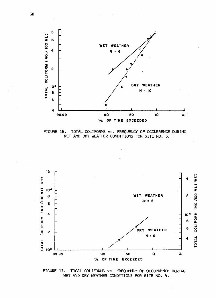
frequency of occurrence for total coliforms, and Figures 18 to 21 to

show the frequency of occurrence for fecal coliforms. Data on fecal

streptococcus, pH, temperature, SS, TDS, TOC, DO, total phosphorus, and

total nitrogen concentrations for the stations may be found in the

thesis by Matsushita (1973).

Geometric mean values were found graphically and listed in Table 6a

together with those parameter concentrations exceeded 10 percent of the

time and 90 percent of the time. These values are listed for each

parameter for each site under dry and wet weather conditions. The range

of log means for all four sites is shown in Table 6b. It appears that

total coliform, fecal coliform, and fecal streptococcus densities are less

during dry weather conditions. Furthermore pH, temperature, TDS, TOC,

T-N appear higher during dry weather conditions. Unlike the arithmetic

mean ranges, the log mean ranges for total coliform and fecal streptococcus

are higher during wet weather and total phosphorus values do not appear

higher for dry weather flows. The extreme values of the arithmetic range

are not evident in the log mean ranges for bacteriological parameters

and bacteriological ratios (FC:TC, FC:FS).

Geometric mean FC:TC ratios ranged from 0.01 to 0.34 during dry con­

ditions and 0.002 to 0.33 during wet weather. Values above 0.20 may

indicate possible contamination from cesspool leakage along the stream.

FC:FS ratios ranged from 0.18 to 2.8 during dry weather and 0.5 to 1.4

during wet conditions. Generally ratios less than 1.0 suggest a pre­

dominance of livestock and poultry wastes while those greater than 2

suggest a predominance of human wastes in mixed pollution. It appears

that dry weather conditions are more apt to have evidence of fecal

contamination from human wastes than wet weather and that wet weather

conditions have evidence of a predominance of animal wastes.

Comparison with State Standards

The parameters were compared with the State of Hawaii Water

Quality Standards as defined in Chapters 37 and 37-A of the Public Health

29

FIGURE 14. TOTAL COLIFORMS (NO./IOO ML) vs. FREQUENCY OF OCCURRENCE DURING WET AND DRY WEATHER CONDITIONS FOR SITE NO. 1.

,... 4 0

..J :2 I , 0 3 / , 0 e/ ....... e t

2 / 0 , , z I :2 le a: " 0 10 4

, "- "e ..J 8 0 u

6 / ..J I ct t , .- , 0 4 DRY WEATHER e " 0 WET WEATHER .- , ,

N = 10 , , N = 6 ,

" , , I , ,

2 99.99 90 50 10

0/0 OF TIME EXCEEDED

FIGURE 15. TOTAL COLIFORMS vs. FREQUENCY OF OCCURRENCE DURING WET AND DRY CONDITIONS FOR SITE NO.2.

0.1.

30

>-a:: 0

:J ::!!! 0 0

" 0 z

::!!! a:: 0 IL.

...J 0 (.)

...J « I-0 ~

8 ..J • 2: 6 I , , 0 ,

WET WEATHER , 0 I

I

4 N = 6 0" " I , 0 ,/e z , , - , , 2: e" , a:: 2

, e" 0 , ,

II. , I

..J "e 0 I , , U I

I DRY WEATHER 104 I ,

..J , e Cl " N = 10 ~ 8

, I

0 ,

I

~ I

6 I ,. ,

e

4 99.99 90 ~O 10 0.1

% OF TIME EXCEEDED

FIGURE 16. TOTAL COlIFORMS vs. FREQUENCY OF OCCURRENCE DURING WET AND DRY WEATHER CONDITI()\lS FOR SITE NO.3.

2

4

104

8 WET WEATHER 2

N = 2 6

4 10 4

,'-" 8 " JI"

,-,1 DRY WEATHER 6 2 ,-

" N : 6 " ,II' 4

,-" ,-

10' I

99.99 90 ~O 10 0.1

0/0 OF TIME EXCEEDED

FIGURE 17. TOCAl COlIFORMS vs. FREQUENCY OF OCCURRENCE DURING WET AND DRY WEATHER CONDITIONS FOR SITE NO.4.

~ l&J ~

..J :E

0 0 , 0 Z

::E a:: 0 II.

...J 0 u

...J « l-0 ~

6 )0-0:: 0

4 ,.. ..J 2 0 0

" 2

0 z

2 102 0::

0 .... 8 ..J 0 6 (,)

..J ~ 4 (,)

ILl ....

2 99.99

WEATHER

• o

N = 6

90

I I , , ,

j I

I DRY WEATHER I i N = 10

50 10

% OF TIME EXCEEDED

31

6

4 .... ILl ~ ,... ..J :::E

2 0 0

" 0 Z

10 4 ..... :::E

8 0:: 0 ....

6 ..J 0 (,)

4 ..J ~ (,)

ILl .... 2

0.1

FIGURE 18. FECAL COLI FORMS (NO. 1100 ML) vs. FREQUENCY OF OCCURRENCE DURING WET AND DRY WEATHER CONDITIONS FOR SITE NO.1.

, , 10 4 , , ,

I

8 • I , , I

I

6 ,

I , I ,

I 4 I

I I I

I , 0 I

..J I I

2 I , 0 2

, f 2 , ,

" ,

o. WET WEATHER I z , , N = 6

, 10 5 ,

(/) I

2 8 ;

0:: , ,

0 I I .... 6 , I

..J I DRY WEATHER I

0 I I

(,) I N= 10 4 :. ..J I , c:t 2

, (,) : . 1&.1

, , .... , , , It , , , , ,

I I

I

102 I

90 50 10 0.1

% OF TIME EXCEEDED

FIGURE 19. FECAL COLI FORMS vs. FREQUENCY OF OCCURRENCE DURING WET AND DRY WEATHER CONDITIONS FOR SITE NO.2.

32

>-0:: Cl

:J ~

0 0 --"-ci Z

:!E 0:: 0 LL

....J 0 u

....J ct 0 loLl LL.

..J ::E 0 0

"'-0 z

:I a:: 0 LL.

..J 0 (,)

..J ct 0 I.LI LL.

4

3

2

104

8

6

4

2

WET WEATHER

N = Ii:>

l I

I I .:

I I

I I

I I

I I

I I

.,' I

I I

I I

I

• : DRY WEATHER l

/ N = 6 I

I :. I

l I I.

99.99 90 50 10 0.1

% OF TIME EXCEEDED

FIGURE 20. FECAL COLIFORMS vs. FREQUENCY OF OCCURRENCE DURING WET AND DRY WEATHER CONDITIONS FOR SITE NO.3.

2 . 2 I -0--

I

o /WET WEATHER I

I I

N = 2 I • 10 3 I

10 4 I I

I

8 I .: 8

I , 6

I I 6 I

I I

I I

4 I

4 I I

I I

I

" I DRY WEATHER I

I I

I N = 6 2 I 2 I I

I I

I I

I I

I

10 2 I

10 3

99.99 90 50 10 0.1

0/0 OF TIME EXCEEDED

FIGURE 21. FECAL COLIFORMS vs. FREQUENCY OF OCCURRENCE DURING WET AND DRY WEATHER CONDITIONS FOR SITE NO.4.

t-w ~

....J ~

0 Q "-0 Z

~ 0:: 0 LL.

:i 0 U

..J <l (,)

w I..L

TABLE Ga. LOG NORMAL FREQUENCY DISTRIBUTION RESULTS.

SITE

Te

Fe

FS

pH

TEJof>

55

TOS

TOC

00

T-P

T-N

Fe:Te

Fe:FS

Te

Fe

FS

pH

TEl'f'

SS

TOS

00

TOC

T-P

T-N

Fe:Te

FC:FS

Te

Fe

FS

pH

TEl'f'

SS

TDS

00

TOC

T-P

T-N

Fe:Te

Fe:FS

Te

Fe

FS

pH

TEI'P

5S

TOS

TOC

00

T-P

T-N

FC:Te

Fe:FS

DRY WEATI£R , OF TIlE EXCI!EDED

.llL

10,000

400

980

7.4S

23.3

21.8

150

13.8

7.8

0.20

0.34

39,500

16,000

24,000

7.5

23.3

16.4

163

8.5

18.8

0,26

0.42

94,000

14,500

11,500

8.25

24.5

54

195

8.0

46

0.285

0.58

4,000

1,000

2,700

8.45

28.5

85

33,500

27.5

7.0

0.74

0.67

3,200

32

150

6.8

20.8

4.3

63.5

6.45

7.05

0.079

0.20

0.01

0.21

8,900

440

2,350

6.95

21.2

6.6

93

7.6

9.1

0.077

0.273

0.05

0.18

23,000

1,660

3,700

7.3

22.8

12

122

7.4

20.5

0.165

0.310

0.07

0.45

1,900

650

230

8.3

25.8

26.5

21,000

12.2

5.6

0.28

0.49

0.34

2.8

1,030

<10

23

6.1

18.0

<2

27.2

3.08

6.5

0.031

0.12

2,000

<100

230

6.4

19.2

2.7

53

5.75

4.4

0.024

0.1]8

5,700

<1,000

1,000

6.45

20.5

<10

23

6.9~

9.2

0.1

0.164

<1,000

<100

<100

8.1

23.5

dO

13,000

5.3

4.5

0.105

0.355

WET WEA1l'£R , OF T11'£ EXCEEDED

58,000

340

160

7.3

21.6

6.9

17.3

6.7

7.65

0.051

0.35

>100,000

2,400

7,800

7.3

20.3

55

140

7.4

6.9

0.235

0.295

83,000

42,000

19,500

7.7

22.0

150

280

7.45

11.7

1.10

0.66

27,000

1,650

1,700

7.8

21.5

49

4,800

17.7

6.80

0.24

0.66

18,000

40

40

6.65

19.5

4.6

100

3.5

7.1

0.02

O.lS 0.002

1.0

9,000

1,130

2,240

6.8

19.5

20.5

70

7.3

4.0

0.105

0.15

0.12

0.50

36,000

12,000

10,500

7.0

20.6

35

112

7.1

4.9

0.28

0.315

0.33

1.14

24,000

1,500

1,100

7.4

21.5

31

2,000

16.8

6.55

0.10

0.40

0.06

1.36

5,550

<10

10

6.0

17.8

3.05

59.0

1.8

6.6

<0.01

0.063

<1,000

520

640

6.2

18.6

7.8

35

7.2

2.3

0.048

0.076

15,800

3,500

5,600

6.3

19.3

<10

46

6.85

2.1

<0.1

0.154

21,200.

1,360

740

7.0

21.5

20

1,000

16.0

6.30

0.043

0.245

33

34

TABLE 6b. RANGE OF LOG MEANS FOR SITES 1 TO 4.

PARAMETERS DRY WEATHER WET WEATHER

TC 37200 -237000 97000 -367000

FC 32 - 17 660 40 -127000

FS 150 - 37700 40 -107500

pH 6.8 8.3 6.65 - 7.4

TEMP 20.5 - 25.8 19.5 21.5

SS 4.3 - 26.5 4.6 35

TDS 63.5 -217000 70 - 2,000

00 5.6 - 7.6 6.55 - 7.3

TOC 6.45- 20.5 3.5 16.8

T-P 0.08- 0.28 0.02 - 0.28

T-N 0.20- 0.49 0.15 - 0.40

FC:TC 0.01- 0.34 0.002- 0.33

FC:FS 0.18- 2.8 0.5 1. 36

Regulations (1968). These regulations classify both coastal and

fresh waters in accordance with the uses to be protected. For coastal

water uses, Classes AA, A, and B were adopted. Class AA waters pertain

to waters used for oceanographic research, propagation of shellfish and

marine life, conservation of coral reefs and wilderness areas, and aes­

thetic enjoyment. Class A waters pertain to waters that are recreational

in nature such as fishing, swimming, bathing and other water contact

sports. Class B waters are waters that are used for small boat harbors,

commercial, shipping, and industrial activities, bait fishing, and aes­

thetic enjoyment. For fresh water uses Classes 1 and 2 were adopted.

Class 1 waters are used for drinking and food processing. Class 2 waters

are those used for bathing, swimming, recreation, growth, and propagation

of fish and aquatic life and agricultural and industrial supply. In

reference to this study, Kalihi Stream is classified as Class 2 waters,

Keehi Lagoon as Class A waters, and Keehi Lagoon marina areas as Class B

waters. Specific standards applicable to these particular water areas

35

were also adopted but those standards pertaining to Class 2 waters are of

specific concern in this study. Class 2 standards include microbiological

requirements, pH limits, dissolved oxygen minimums, and radionuclide

requirements. Bacteriological requirements pertain to coliform and

fecal coliform densities. The median coliform should not exceed 1000 per

100 ml nor should more than 10 perce~t of the sample exceed 2400 per 100

mI. Fecal coliform content should not exceed an arithmetic average of

200 per 100 ml during any 30-day period nor more than 10 percent of the

samples exceed 400 per 100 ml in the same time,period. pH units should

not be less than 6.5 nor higher than 8.5. Dissolved oxygen should not

be less than 5.0 mg/l. There are no requirements for nutrient materials

in fresh waters.

In Figures 3, 4, 7, and 8 showing seasonal variations from October

1971 to August 1972, a number of samples did not meet the State require­

ments. Total coliform values were greater than 1000 per 100 ml through­

out most of the study except during February to May. Fecal coliform

values were greater than 200 per 100 ml throughout the study with the

exception of Site No.1. Sites No. 1 and No.2 had pH values less than

6.5 throughout most of 11 months and Site No. 4 values dropped below

5.0 mg/l DO on one occasion.

In Table 6 showing the range of geometric means during dry and

wet weather conditions, coliform values for 50 percent of the samples

exceeded 3200 coliforms per 100 ml during dry weather and 18,000 per

100 ml during wet weather. For Site No.2, 50 percent of the samples

exceeded 8900 per 100 ml for dry weather and 9000 per 100 ml for wet

weather flows. Site No.3 values exceeded 23,000 coliforms per 100·ml

in 50 percent of the samples for dry weather and 36,000 coliforms per

100 ml in wet weather. Similarly, Site No. 4 exceeded values of 1900

per 100 ml and 24,000 per 100 ml during dry and wet weather, respectively

for 50 percent of the samples. Geometric means for pH and DO were within

the limits of the standards.

It can be seen on extrapolation of the log normal frequency distri­

butions that 90 percent of the samples exceed 100 coliforms per 100 ml

during dry weather and more than 98 percent of the samples during wet

weather for Site No.1. For Site No.2, 97 percent and 83 percent of the

36

samples exceed 1000 coliforms per 100 ml during dry and wet weather,

respectively. For Site No. 3 more than 98 percent of the samples exceed

1000 per 100 ml during dry and wet weather. Finally, Site No. 4 values

exceed 1000 per 100 ml in 86 percent of the samples during dry weather and

98 percent during wet weather. Fecal coliform values exceed 200 per 100

ml in approximately 17 percent of the samples during dry and wet conditions

for Site No.1. For Site No. 2 fecal coliform values exceed 200 in 60

percent and in more than 98 percent of the samples during dry and wet

conditions. For Site No. 3 the values exceed 200 at least in 80 percent

of the samples during both conditions. Finally for Site No.4 the

values exceed 200 in 83 percent and 98 percent of the samples during dry

and wet conditions. pH values were below 6.5, in 1 to 30 percent of the

samples for all four sites during both dry and wet conditions. DO values

were within the limits of the State Standards with the exception of Site

No.4 where for 25 percent of the time. DO values were below 5.0 mg/l.

In evaluating nutrient levels, samples were compared with Class A

nutrient standards that apply to Keehi Lagoon since there are no nutrient

requirements for Class 2 waters. Nutrient materials are identified as

total nitrogen and total phosphorus in the State Standards with the

former not to exceed 0.15 mg/l and the latter, 0.025 mg/l for Class A

waters. The range of log mean values for total nitrogen and total

phosphorus exceeded the Class A standards under both dry and wet condi­

tions for each site along the stream. Total nitrogen values ranged between

0.20 and 0.49 mg/l during dry weather and 0.15 and 0.40 mg/l during wet

weather. Total phosphorus ranged between 0.08 to 0.28 mg/l during dry

weather and from 0.02 to 0.28 mg/l during wet conditions.

Comparison with Other Investigators

Generally, arithmetic mean values obtained in this work are within

the limits of other studies performed in the u.S. for parameters such as

pH, specific conductance, chlorides, nitrogen forms, total phosphorus,

DO and TOC. However BOD, turbidity, total solids and suspended solids

in Kalihi Stream samples are considerably lower than the ranges show.

Bacteriological values were within the same magnitude as other studies in

37

the U.S. but were on the low extreme end of the range. This is further

evident in Table 7 which shows the bacterial counts which are exceeded by

10, 50 and 90 percent of the samples. Although Kalihi values are high

in the 90 percent column they are well below others in the 50 percent and

10 percent columns.

TABLE 7. BACTERIAL COUNTS IN RUNOFF SAMPLES FROM URBAN AREAS.

LOCATION

CINCINNATI, OHIO (NELSON, 1963)

TULSA, OKLAJ-lOMA (DEPT. OF HEALTH,

1968)

KALIHI STUDY

COUNTS EXCEEDED IN DESIGNATED SAMPLES (COLONIES/100ml)

BACTERIOLOGICAL PARAMETERS

TC

FC

FS

TC

FC

FS

TC

FC

FS

90%

2,900

500

4,900

2,100

2

2

10,880

1,340

1,770

50%

58,000

10,900

20,500

57,000

30

5,000

21,700

3,670

3,470

10%

460,000

76,000

110,000

1,140,000

30,000

167,000

67,000

11,600

7,290

% OF

Ka1ihi Stream results were also compared with investigators in other

countries (Table 8). Generally, BOD, total solids, suspended solids, and

total coliform densities were less than the values found in other studies.

The Kalihi Stream results were compared with other investigations

in Hawaii. Generally, all values showed considerable agreement and

closeness in all categories (Table 9) particularly with Quan et aZ. (1971),

Ching (1972), and the unpublished Faculty Housing data. The similarity

of range values is exemplified by the Faculty Housing data. During wet

weather flows, Kalihi Stream samples demonstrated the following ranges:

TABLE 8. COMPARISON OF THE QUALITY OF URBAN RUNOFF IN KALIHI STREAM WITH RESULTS OF OTHER STATES AND COUNTRIES.

l.OCATtCJ4

.:ALIHI, HotMUl 1912

D!'rnOlT, M1O'tI~

PAIJoO, 1,.., ~ AAICR, .... on-. leItIe, a:JtaQ-W:Je:, 1966

SEATTl.E, *9iJfC.TCIt

5l'L\II!S1BI:, NCIEISCIt, 1,"

C"CI~TI, QflO

!ellln £T ~ 196213

CUCI,...,n, 000 (JAIN)

N!!11a. fT M.. 1966

cowe .... IN\'IAG

HIT'11WII, MSDC., 1_

M..I5Tltt TOM

PItLIi, e. Q.5, 19M

...-oex,1DIoS ~n ... ATUlHTA,. Ci8l5lA

1UOt, CXIi', llD!5lGS

1MliIHSK!, V1KlHIA

~m. S!A1, *'~, 1970

OIlrA&O, ILLumlS -lILSA, oa..tIOO\

IWCIJ, 1967 ....

...... N. CMCI..IMl _ ..... 19M

.-cz, .-... ,ffC1Ie, 1,""""

u:a .tHZI.a, CAU~A

ItJ2-)2

'"7-sa 1M2-4' MIISHIICTt'II, D.C. "_, IiMSttUCTOI, D.C.

WIUPP'l !T M., 19M CIINY, __

VlLJttNSat, 1154

S1CQOQJO, -...

MBtUfOI, l'-~

S1CQOQJO, -­

sIIDawI>, "" HDSCQI, U5SIl

11M LJ!NItU,tI), U5SIl

I_51 _, ussa

PM\QtfINSICY, 1_

PII!l1lIII" s . ...,co $TJfCI!R, 1"1

WCRTS, CiIO.ID MIA

A!51a!MT1M.. PMII:5

eu51teSS, PlAT AA!M

............ ItI..ImIEIL. 1961

~

ST'METS IN COMt8I --CITY

STlI£ETS ""--;aos

IX> BOO. TOt en- T1J ?J

6.35 0.15 1 -7.5 ).75 11

96-... 10 1,290 ,so

1-

'" 20- JO·I0·

6.' - 10-9.0 n

20

'" - 159-I'S SII

610 1,,011 It6I

16

, -..

1- 15- 1t2-

11 .... lSI .... . " -"toO m

1.0 I.'

'.0 '.2 7.' 11.1

I -US

J -90

lit

10

<, I. -m

56

12.' -1'5

10

.. 1.1It -

12 , -.. . -95 %6-

10

21-

"

.. -I"SlIit

',100

.. 21

SP!C.

" TQS "IS S$ 't'S5 SETT. S. 50-. FI'O.t T~ N A»'S Cl coo. ... n: '" .. 310 -

.. 0

10-

',,1S1

".

10 -

.n 1.6 -

"' I ....

5 • 1-

1,,200 200

n '.1

so -123,100

20- 52- 20-

l .. ilIS 2, ..... l"M

In 10'

'" - n - ... -I,N.... 2,052

U-

m ... _ .. - 71-

lIt,t2I nJ 9tS

'" -IIt,6OO

J,OII

... 1"

I,JJII

I .. '''' I,M

%6-56,2S0

12- 150- 1- 0-

1,00IIt 16 .. 111 100 7.6'IG

2,&\S

1 .. 000 •

),SOt

II1t,Sltl

It5I - IS-

S .. DOe 6D\

<0.02 ..

l.J

0."

0.5'* •

I."

1.01 _ 0.01 - lit - IfI.2 - '.1 - 100 .. I .. 200 -

I.GIt 1.0- '75 1,010 I.DS 115,001 lOD,_ 21,_

25,001 -

1.' t.R

1." 11.1

0.) .. ) -

7.' UI I.J

0.1 - 0.0-

S.J 0.1

t.J -1.6

<I -llIt.O

0.1 - 1It.'-..... It

m

,11

s.) -1.1

0.1

,.) .. I.J

7.0 ..

1.1

5.\ -

1.0

i.l ..

1.1

no,DOG 1,210,"

Ii, 100

In,GOO

0 •• - 2 .. ".. '.1.. 5," -

I ./t. '" 220 1.1t 'OO,ooe 0.53 - .. -

2.1t I' 2.7- GoO '.J-1.\ 57 1.1

20.0

"., 11-

150

a,1OG lltO,OOO

11- 100-

11,000 30,000

0.1 - 1.5- 6.0 • 120 .... ~ ltCi"OOO - ',,100 ~

1It.5 '.5

<0.1

,.It .. J2

7.2 5,,200,DOI 1,,5OG,,00I 60 .. 000

"',DOG

IO,DOG

25 .. 010 -

2SO,DOG

N,OII

nt,DOG

.... ~l"lC!

0." -o.n t.2I

1.2ft •

2.1t'

VI 00

TABLE 9. COMPARISON OF THE QUALITY OF URBAN RUNOFF IN KALIHI STREAM WITH RESULTS OF INVESTI­GATORS IN HAWAII.

LOCATICII 00

QUAN, YCUG ET PJ.. (1968)

~Ct£ SllIE»I .oK)

KEAPH<\LA STREN4S (970)

HNfl (968)' - 18.7 'tW'1>UW>. S'IRENI

ClASS 2

YCUG (1971)

'tW'AlRIA STREAM

CHING (1972)

IW«lA STREAM ClASS

2 WATERS

DRY IEAlHER 6.55 - 8.44

WET WEA1HER 6.96 - 8.~

KALIPI sT\.O'(l (1972)

DRY WEAlHER 5.8 - 8.()X

WET WEAlHER 6.6 - 7.3"

0t.N, YCUG, .oK) NaRSCJI 0.972)

FACULTY HS6 G.N"JB.) RAIN, BIG ISLfH) Q 957)

RAIN, Cl.'HJ (1972)

LOCATICII

QUAN, YOlNi ET AI. (968)

~Ct£ STREAM .oK)

KEAAHAI.A STRfIIIoIS (970)

HNfl (968)'

'tW'AIJ'I1A SllIE»I

ClASS 2

YOl.NIi (971)

'tW'AIJ'I1A STREAM

tHINIO(1972)

IW«lA STREAM CLASS

2 WATERS

DRY WEAlHER

WET WEAlHER

KALIHI ST\.OY'(1972)

DRY WEAlHER

WET WEAlHER

C1

n - 121""

15.3 - 24.6

11.0 - 15.9

21 - 31x

20.5 - 27.0

0t.N, YCUG, />H) AI'aRSctI (1972)

FACULTY HSG (IN'UB.) - 39

RAIN, 81G ISI.JIK) 095])

RAIN, Cl.'HJ (972)

, STATICtIS PBCNE TICA1. GATE

16

4.7

BOO TOC TU cu

0.3 - ItS.O

2.8 - 32.0 6.2 - 11.0

~2 - 59 lB.3 - 35

0.35 - 2.2'" 10.7 - 22.0 ~.2 - 11.8

0.35 - 2.5()X 3.5 - 17.0 16.3 - B6

2.5 - 19.0 45 - 120

SPEC C pH T9'P ·C TC

7.8 - 8.6 21 - 25

6.6 - 9.0 800 - 110,000,000

20.8 - 29.5 -

6.~ - 7.55

7.01 - 7.50

100 - 214X 6.7 - 8.25

65 - 119 6.7 - 7.6

79 - 149 6.9 - 7.9

5.2 - 6.3

6.6 - 6.8

20.5 - 25.0

20.1 - 23.~

19.9 - 26.2

19.1 - 21.5

13,000 - 21,-000

22,000 - 43,000

3,200 - 23,000

9,000 - 36,000

200,000

, AAlTl-t'ETIC _ RJINGES EXCEPT BPCIERIAI. t£NSlTIES (GEO£TItIC _ RJINGES)

EXCUDING STATItN 4, SALT WATER INTRUSICII

CNH,-fI + 1IJ,-fI) xx

EXCJ..lI)ING TICA1. INFU.ENCES

TS ms 55 T-P T-fl

0.001 - 0.07 0.05 - 0.60

ASIIJ,-fI

100 - ~70"" - 0.1 - 2.5 - 11.8

- 36

po,

102 - 18~ 6.~ - 30.1 0.23 - 0.~3 0.20 - 0.30

190 -260 88 - 117 0.57 - 0.66 0.23 - O.~

T-P

88.4 - 1~9" 82 - 128 6.11 - 37.2 0.11 - 0.3~ 0.24 - 0.~3

105 -2~ 73 - 181 ~.~ - ~.O 0.03 - 0.27 0.10 - 0.6't

105 - 330 0.06 - 0.25 0.01 - 0.33

0.06 - 0.08'

Fe FS PC/PS PC/PC

0- 7,000 -

200 - 9,300,000 100 - 5,400,000 5.2 0.25

140 - 2,000 2,500 - Ilt,OOO 0.005 - 0.093 0.27 - 0.59

720 - 2,600 6,000 - 18,500 0.033 - 0.14 0.17 - 1.06

32 - 1,660 150 - 3,700 0.11 - 2.8 0.01 - 0.3'<

40- 12,000 40- 10,000 0.5 - 1.36 0.002 - 0.33

10,000 154,000

~ ~

40

3.5 to 17.0 mg/l TOC, 105 to 246 mg/l TS, 0.03 to 0.27 mg/l T-P, 0.10 to

0.64 mg/l T-N, 20.5 to 27.0 mg/l Cl-, 65 to 119 ~mhos/cm specific conduct­

ance, and 6.7 to 7.6 pH units. These ranges compare favorably with

Faculty Housing data values of 2.5 to 19.0 mg/l TOC, 105 to 330 mg/l TS,

0.06 to 0.25 mg/l T-P, 0.01 to 0.33 mg/l T-N, 8 to 39 mg/l Cl-, 79 to

149 ~mhos/cm specific conductance, and 6.9 to 7.9 pH units. However,

bacteriological values were lower for Kalihi Stream samples compared with

the Faculty Housing data.

Some results may have differed from the range of other investigators

in the U.S. and other countries because of .a number of factors. Hydrologic

factors such as imperviousness, elevation, basin shape, length of main

stream, and ground cover will alter stream flow. Precipitation character­

istics differ in different areas. Such characteristics as rainfall dura­

tion, volume and intensity, temperature, wind conditions, and length

of time since the last event will vary according to geographical locale.

Environmental and human activities such as street maintenance, air

pollution sources, drainage system conditions, traffic volume, con­

struction, recreational events, condition of housing, industrial

contributions, and land uses differ in different states and countries.

These variables may affect the flow volume and parameter concentrations.

Results were similar to Hawaiian investigators probably because

a large number of these factors are similar. Most hydrologic factors

are similar with regard to geological characteristics as well as most

precipitation characteristics. In general most environmental and human

activities are similar with some variations in street traffic, litter,

housing conditions, industrial contributions, construction, and land uses.

Comparisons Under Dry and Wet Weather Conditions

Geometric mean values of the various parameters were compared with

the length of the stream for dry and wet weather flows in Figures 22 to

32. Total coliform, fecal coliform, and fecal streptococcus densities

were higher during wet weather conditions for all sites. pH, TDS, and·

temperature values were found to be higher during dry weather for all

sites. DO values were higher during dry weather flows for Sites 2 to 3

but decreased below wet weather values at Site No.4. TOC was higher

during dry weather for Sites 1 to 3 but were lower at Site No.4.

SS values were markedly higher during wet weather conditions for all

sites. The nutrients, total phosphorus (TP) and total nitrogen (TN),

have contr~sting trends. T-P appears to be higher during wet weather

conditions while T-N values with the exception of Site No. 3 are higher

during dry weather conditions.

Hydrograph-Concentration Relationships

Continuous sampling was conducted at Site 1, 2, and 3 during high

and low flows. Eight sampling runs were performed, one run at Site 1,

three at Site 2 and four at Site 3. Three samplings at Site 3 traced

peak flows for 7, 12, and 9 hours. Flow data for Site 3 were plotted

against time and correlated with parameter concentrations of SS, T-N,

41

and T-P as shown in Figures 33 to 40. Sites 1 and 2 showed no significant

hydrograph-concentration relationships.

Three characteristic trends seem evident in all hydrographs. The

peak concentrations lag behind the peak flows. It also appears that some

concentration peaks precede the peak flow in a number of instances during

the rise of the hydrograph. This may be some first flushing action of

.... ..J 105 ::I o 2 "-o 104

Z

::I a: 10 5 o .... ..J o o ..J C I­o I-

DRY WEATHER

LENGTH OF STREAM IN 1000 FEET

FIGURE 22. TOTAL COLIFORM DENSITIESlJ'.lDER VARIOUS WEATHER CONDITIONS ALONG COURSE OF STREAM.

10 7

-- 10' ..J :I 0 0 ....... 10 5

0 Z

:I 10 4 II: 0 I&-..J 0 (,) 103

..J 4 (,) I&J Ii.. 10 2

,,4, ~~ .. #" ..

WET WEATH ER ...... ~~ ' .. ,,# ,

, , , , , ,

*" " ,o-~""" -----..... 'b

" ,'/ /' DRY WEATHER

"", d'.

30 25 20 15 10 5 o

10 7

--..J :I o 10' o ....... o Z 105

en :;) (,)

(,) 10· o u o t-A-W II: t-en

10 3

..J 4 (,) 10 2 I&J Ii..

WET WEATHER

/" " ,,/ DRY WEATH E R

/ (//

30 25 20 15 10 5 LENGTH OF STREAM IN 1000 FEET LENGTH OF STREAM IN 1000 FEET

o

FIGURE 23. FECAL COLIFORM DENSITIES UNDER VARIOUS FIGURE 24. FECAL STREPTOCOCCUS DENSITIES UNDER WEATHER CONDITIONS ALONG COURSE OF STREAM. VARIOUS WEATHER CONDITIONS ALONG COURSE OF STREAM.

.j:I. N

l: A.

9.~

9.0

8.5

8.0

7.~

7.0

6.5

6.0

DRY WEATHER ,-

--_ ... --------------------_ .. --0---------

WET WEATHER

,P ,

" ,-

30 25 20 15 10 5 0

LENGTH OF STREAM IN 1000 FEET

FIGURE 25. pH UNDER VARIOUS WEATHER C()\IDITI()\IS ALONG COURSE OF STREAM.

u o

I&J

26

25

24

23

a::: 22 ::::> .... oe( a::: I&J a... 2 21 I&J ....

20

19

DRY WEATHER

.... , .. .. ' .. ' ....

, .. .... .... ",

,JS

,P ,/ ., ,-

0-------------0',,'" WET WEATHE·R

30 25 20 I~ 10 5

LENGTH OF STREAM IN 1000 FEET

FIGURE 26. TEMPERATURE UNDER VARIOUS WEATHER CONDITIONS ALONG COURSE OF STREAM.

o

~ VI

8.0 r DRY WEATHER

J 75 [ ~4'_ ~ •• ::-~ WE A ~-~-~:----------~~

....... 7.0 C)

::::E , ". z ~ 6.5 ~ X 0

0 w 6.0 > ..J 0 U) U)

c 5.5

5.0 30 25 20 15 10 5 0

LENGTH OF STREAM IN 1000 FEET

FIGURE 27. DISSOLVED OXYGEN UNDER VARIOUS WEATHER CONDITIONS ALONG COURSE OF STREAM.

30

25

..J ....... C) 20 :=E

z 0 CD ~ 15 4 0

/ 0 DRY WEATHER z

/ 4 10 C) ~ I 0 I

I

..J / 4 WET WEATHER.J t- 5 0 ~----------.-------t- 0-------.---

0 30 25 20 15 10 5

LENGTH OF STREAM IN 1000 FEET

FIGURE 28. TOTAL ORGANIC CARBON UNDER VARIOUS WEATHER CONDITIONS ALONG COURSE OF STREAM.

0

~ ~

0.6

0.5

--..J ..... (!>

2: 0.4

(/) ::l 0: ~ 0.3 Q. (/)

0 ::E: Q.

0.2 ..J ~ I-0 I-

0.1

,A , \ , \ , \ ,- \

WET , \

WEATHER ,/ \

" 0-' "

30

" "

25

"d "

",'

20

"" ,-,'-

""

WEATHER

15 10 5 LENGTH OF STREAM IN 1000 FEET

o

FIGURE 29. TOTAL PHOSPHORUS UNDER VARIOUS WEATHER CONDITIONS ALONG COURSE OF STREAM.

0.6

0.5

..J ..... (!>

2: 0.4

z 1&.1 (!>

0 0: I- 0.3 z ..J ~ I-~ 0.2

0.1

DRY WEATHER

,-,-,,-, " " ,,,,,,

" ,/ WET WEATHER 0------------0'

30 25 20 15 10 5 LENGTH OF STREAM IN 1000 FEET

o

FIGURE 30. TOTAL NITROGEN UNDER VARIOUS WEATHER CONDITIONS ALONG COURSE OF STREAM.

~ til

60

50

...I

" (!)

~ 40

CI) 0

...I 0 30 CI)

0 1&.1 0 Z 1&.1 20 a.. CI) :::) CI)

10

WET WEATHER

"

e{ ,'­.-

" ",,'

I'

/

" "

" " "~,,,

"

",~ ...... " .... -' .... "" ......... 0

(j DRY WEATHER

30 25 20 15 10 5

LENGTH OF STREAM IN 1000 FEET

o

FIGURE 31. SUSPENDED SOLIDS UNDER VARIOUS WEATHER CONDITIONS ALONG COURSE OF STREMv1.

en o ...I o CI) 15 o 1&.1 > ...I o ~ 10 o ...I

'" I-o I- 5 DRY WEATHER

30 25 20 15 10 5 o LENGTH OF STREAM IN 1000 FEET

FIGURE 32. TOTAL DISSOLVED SOLIDS UNDER VARIOUS CONDITIONS ALONG COURSE OF STREAM.

~ ()\

22 240 120

20 ~ -I 200 100

..J

16 ~ -t 160 ....... C) 80 2

(I) (I) IL. IL. t"'tt u u (I)

0 , I

I \ 12 Q 120 ..J IIJ 60 ; ss IIJ 0 (!) (!)

, I (I) , I a: a: , .\ « « ,4

, 0 ,

X X , ,

IIJ , ~

I U u ~ , 0

(I) (I) , , z , ,

1 ~ 80 40 8 , IIJ 0 0 , t I Q. , I , , I

, (I)

I I I :> , I

• I , , (I)

I I I , , I I I , I I , I ,

4, : I I I I I I I 40 20 4 .- 't1 I I , I I , I I , , I , I I , I I I

I I , I

t " u 'A"

I

2 4 8 12 16

TIME (HOURS)

FIGURE 33. DISCHARGE-SUSPENDED SOLIDS vs. TIME AT SITE 3.

."A ... ' , -I I ' ~

, , , , , I

I , , , , , , , A ; •

~ • I • , , , • • • \

, • , I

• , • I , • I ~ I

\ • , • • , , I Q I ,

SS I I I

\ I , , I I , I

A ,

~ , \ ,

I

\ , ,

\ , \ , \ ,

I \ , , ~ t , , , , , ,

I , , , , , , , A, , l-,

\ I \

~ I , / , , ,

\'IY/ '~ -I "2t.... .. ....

AA

4 6 8 10 12 TIME ( HOURS)

FIGURE 34. DISCHARGE-SUSPENDED SOLIDS vs. TIME FOR SITE 3.

240

200

160

120

80

40

..J ....... C)

2

(I) 0

..J 0 (I)

0 IIJ 0 z IIJ L (I) ;:) (I)

+>­~

160 320

~ 00

,~ -, 280 I I

140 I , , , I I , , ,

120 240 24 r .., 1.2

-"

...J

100 l-"

-I 200 '" 20 -f 1.0 (!) ,I

:IE II I I , I - , I I I U)

U) I I

~ ...J "-

0 : I T- P

'" 0

i \ 80 160 ::; U) 16 0.8 ;

0 "- (t U) 0 , I W , I : I (!) Q SS 0 1\ I I 0::: I I : I U)

<l W W : , , I ;:) :r 0 (!) I I I I 0::: 0 Z 0::: I : 0

120 ~ 12 I ' I 0.6 :z: U) 60 <l I : I 25 U) :z: , I Il.

0 I I U) ;:) I I

U) I 0 U) I I 0 I I :z: ,

Il. , I I I I I ,

I I I I

, 0.4 ...J 40 l- \. -I 80 8 l- I I I c( ,

I , I I I I I l-I I A 0 I I I I , l-I

~ ~ :

I , I ¢.. I , I ~_#-lt : I , I , I

I , I I I , p' ,: , t , I

1 I ,

I \ d , A.." " I , I I

~" ..J 0.2 20 l- I I I , 40 4 ... n-... ..:l \ : \ I , I I I

't{' , , I I

I I , , I \ , I

,A I

~;~, I

Ib, lb, , , I , IS. ,

, '-i:f '~ ~, , , 4 "'_tz._ A - A '_A..' I L

2 4 6 8 10 4 8 12 16

TIME (HOURS) TIME (HOURS)

FIGURE 35. DISCHARGE-SUSPENDED SOLIDS vs. FIGURE 36. DISCHARGE-TOTAL PHOSPHORUS vs. TIME FOR SITE 3. TIME FOR SITE 3.

(/) I&.. U

III <lJ a: C( :I: U (/)

o

120

100

80

60

40

20 ~ , , ,

\ \ , ''1:1

2

6 , , I I I • I I I I I I I I

I I T-P I I

I I

Q i~l , '. '. , , I , , , , , : : , I I , , , , ,

I , , I I , I

4 Po, \ : \

I, I \. "ii;' ~

\ I \ I I

\ ,LI.-'A, 'n--A.'n b' \ tJ.. '-4,

\ , ~ I ,

'6'

4 6 8 10 TIME (HOURS)

FIGURE 37. DISCHARGE-TOTAL PHOSPHORUS vs. TIME FOR SITE 3.

4.8

4.0

..J

"­<lJ

3.2 2

(/)

~ a: o :I:

2.4 a.. (/)

o :I: a..

..J C(

1.6 I­o I-

0.8

(I) I&.. U

III <lJ a: C(

:I: U (/)

o

24

20

16

12

8

4

~ .. , " : " : 't) I I , I I \ I I

A I I I I "I , , ., , , ,

I , I \ ,

: \: 'tI : \~

tl

4

(.-"4 , \ , I , I , , I ,

P'-N \ I , I , I , I I I I I , I I , ,

I , I I I I , \ ~ , .. \

'4 Q ,

8 12

TIME (HOURS)

16

0.30

0.25

..J 0.20 "­

<lJ 2

Z III <lJ 0.15 0 I:: I-Z

..J • 0.10 l-

e

0.05

FIGURE 38. DISCHARGE-TOTAL NITROGEN vs. TIME FOR SITE 3.

01:>0 \0

(/)

\&.. (.)

~ ~ a:: <t :z: (.) (/)

o

120

100

80

60

40

20

2

~. I , I , I , I ,

I 4 I \ I \ I \ I \ I \

: T -N .. I \ I ,

A \ I \ I ,

' ! \ ''l:f' \ ~\

\4'_~-A-..A._~

4 6 8 10

TIME (HOURS)

FIGURE 39. DISCHARGE-TOTAL NITROGEN vs. TIME FOR SITE 3.

1.2

1.0

0.8 ...J ....... ~

:IE

z ~ 0.6 ~ o a:: I-

z

...J 0.4 ~

0.2

o I-

(/) \&.. (.)

120

100

80

~ 60 ~ a:: <t :z: (.) (/)

o 40

20

I I I i\ I

I , I I \ tl : b..'4,~, I

Ii

2

\

• • , • ,

Q

• I

• I

• I ,

Z{

4 6

A I , I I I , I , I , I , I , I , I ,

I • ; ~ I • I • ~ ,

I 4 : T - N \ I '

I • I ' .. : \ ,I:l--6. ~tJ.' '.B'

•

8

TIME (liOURS)

FIGURE 40. DISCHARGE-TOTAL NITROGEN vs. TIME FOR SITE 3.

10

1.2

1.0

...J .......

0.8 ~ :IE

z ~ ~ 0.6 0 a:: I-z ...J

~ 0.4 0 I-

0.2

(J1

o

runoff from separate storm drainage systems and other sources. Finally

it seems that samples taken at peak flows are lower in concentration of

T-P, T-N, and SS, a seeming dilution effect but actually attributed to

lag time in the peak concentration.

The time between peaks has been estimated for SS, T-N and T-P at

Site 3. For SS, time between peaks ranged 1.5 to 3.0 hours. For T-P,

51

1 to 2 hours and for T-N, 1 to 3 hours. However, time between peaks may

vary depending on a number of factors such as antecedent rainfall, rainfall

intensity and distribution, geologic characteristics, degree of first

flushes, runoff volume and velocity and location of separate sewer inputs.

Comparison with Increased Urban Activity

The four sampling sites were described previously in terms of subbasins

and land use activities concerning undeveloped lands and developed lands,

residential and commercial-industrial areas, schools and recreational

areas, streets and highways, and population and housing densities. In

summarizing the urban activities, there is a general increase in all of

these activities including population and housing densities along the

length of the stream from Site No. 1 to Site No.4.

The general trend for both wet and dry weather conditions for the

different water quality parameters is an increase in total coliform

densities, fecal coliform densities, fecal streptococcus densities,

pH temperature, TOe, T-P, T-N, SS, and TDS along the length of the

stream from Sites Nos. 1 to 3. Between Sites 3 and 4, all bacterial

densities decrease apparently from a lesser degree of contribution of

bacterial colonies in this area or some toxic effect of the receiving

waters which are higher saline.

The average parametric loads based on arithmetic mean concentrations

and average dry and wet weather flows were calculated for Subbasins 1 to

3 (Table 10). Loadings for each subbasin increased in a downstream

direction during both dry and wet weather conditions. Total nitrogen

loads increased from 0.22 1bs/day to 9.0 1bs/day during dry weather

and from 3.58 to 97.3 1bs/day during wet conditions. Total phosphorus

loads increased from 0.11 to 4.2 lbs/day during dry conditions and from

TABLE 10. AVERAGE LOADINGS BASED ON ARITHMETIC MEAN CONCENTRATIONS. V1 N

SITE t-«:>. 1 SITE t-«:>. 2 SITE t-«:>. 3

DRAINAGE MEA (ACRES) 358.4 1,670.4 3,354.9

(SQ.MI) 0.56 2.61 5.24

LB/YR LB/DAY LB5/ACRE/DAY LB/YR LB/DAY LB5/ACRE/DAY LB/YR LB/DAY LB5/Aalf./DAY DRY WEATl-ER

AVE. DI5Q-1. OF 5TREftM (mgd) 0.12 mgd 2.21 mgd 3.02 agd

TOTAL N 80.3 O. 22 (0.219) 1,837.6 5.34 0.17) 3,286.4 9.004 (0.986)

T-P 40.2 0.11 (0.11) 699.0 1.92 (0.402) 1,535.8 4.206 (0.475)

Cl 7,665 21.0 (21.4) 158,451 434.1 (94.9) 28,054.7 768.6 (83.6)

55 2,222.9 6.09 (6.21) 48,600 133.2 (29.2) 197,247 540.4 (58.8)

TS 32,302 88.5 (90.2) 767,372 2,102 (459.5) 1,372,166 3,759.4 (409.2)

BOO 131.4 0.36 (0.3]) 6,667 18.3 0.98) 10,081.1 27.62 (2.99)

TOC 4,197.5 11.5 (11.68) 72,319 198.1 (43.4) 201,690 552.4 (60.2)

Na 6,146.6 16.84 07.2) 134,816 369.4 (80.]) 322,232 882.8 (95.99)

K 719.1 1.97 (2.01) 13,899 38.1 (8.40) 43,840 120.1 03.14)

Fe

Cr 25.6 0.07 (0.073) 274.7 0.752 (0.183) 437.8 1.19'!! (0.146)

Al 25.6 0.07 (0.073) 558.6 1.528 (1. 329) 875.3 2.40 (0.256)

WET WEATHER

AVE. DISQ-I. OF STREftM (mgd) 4.17 mgd 22.25 mgd 30.9 mgd

T-N 1,306.7 3.58 0.65) 1,127.9 3.09 (6.94) 35,511 97.3 (10.55)

T-P 394.2 1.08 0.09) 7,533 20.64 (4.38) 47,298 129.6 (14.09)

C1 260,318 713.2 (726.4) 1,419,212 3,888 (850.5) 2,534,819 6,944.7 (755.6)

55 55,845 153.0 055.8) 2,147,727 5,884 (1,284.8) 6,083,689 16,667.6 (1,814)

TS 1,466,570 4,018 (4,091.6) 7,083,72E 19,407 (4,241. 3) 23,100,185 63,288 (6,884)

BOO 4,453 12.2 02.4) 43,987 120.5 (26.3) 126,730 347.2 (37.6)

TOC 44,348 121.5 (123.]) 276,322 757.1 (164.3) 572,857 1,569.5 (170.8)

Na 571,663 1,566.2 0,595) 1,893,961 5,188.9 (1,135.2) 4,038,767 1l,065 (1,204.5)

K 82,417 225.8 (229.9) 175,870 481.8 (lOS .1) 490,050 1,342.6 (I46)

Fe

Cr 1,138.8 3.12 (3.1]) 2,008.5 5.50 (1.20) 5,576 15.28 (1.68)

Al 890.6 2.44 (2.48) 6,023 16.50 0.61) 9,464.6 25.93 (2.81)

53

1.08 to 129.6 lbs/day during wet weather. SS loads and TOC loads

ranged from 21 to 769 lbs/day and from U.S to 552.4 lbs/day, respectively

during dry weather and from 153 to 16,668 Ibs/day and from 121.5 to 1,570

lbs/day, res:(,ectively, during wet weather flows.

Annual contributions of SS ranged from 2,223 to 197,247 lbs during

dry weather flows and 55,845 to 6,083,689 lbs during wet weather flows.

For T~N and T-P loads during dry weather flows there was a range from

80.3 to 3,286 lbs and from 40 to 1,536 lbs, respectively and during

wet weather flows the range was from 1,307 to 35,511 lbs and from 394 to

47,298 lbs, respectively.

Comparison of Loads with Other Investigators

The loads were compared with Weibel, et aZ. (Cincinnati) (1964, 1966),

AVCO Economic Systems (Tulsa) (1970), Bryan (North Carolina) (1970), Ching

(Hawaii) (1972) and the Consortium for the Oahu Water Quality Study (1972)

(Table 11). The results of this Kalihi Study compare very closely with

the work reported by Weibel, AVCO and Bryan. However, although the

values are within the same magnitude as Ching, there are generally on

the lower extremes of his range of values. Kaneohe Bay and Pearl Harbor

nutrient loads based on average storm flows were generally lower than

those found in this study although West Loch streams had comparable

ranges of total nitrogen and total phosphorus.

Pesticides

Pesticide samples were analyzed on three occasions at each sampling

site. Residues of dieldrin, Y -chlordane, and 0 ' , p'-DDE were detected

but were in the very low ppt ranges. Aldrin, heptachlor epoxide, S-BHC

lindane, DDE, 0', p'-DDT, DDD, DDT, heptachlor, a chlordane, and 0' ,

p'-DDD residues were not detected. Dieldrin was present at 1.75 ppt

at Site 2 on one occasion, 0', p'-DDE, 0.33 ppt at Site 4 on one

occasion and Y -chlordane 1.13 ppt at Site 3 on one occasion.

These values were within the range of pesticide residues found by

Bevenue et aZ. of non-potable waters on Oahu. For streams on Oahu,

TABLE 11. LOADINGS IN KALIHI STUDY AND BY OTHER INVESTIGATORS DURING WET WEATHER CONDITIONS.

x

KALIHI STLOY

(LBS/ACRE/YR)

(LBS/ACRE/DAY)

(LBS/DAY)

WEIBEL ET AL (1964, 1966)

(LBS/ACRE/YR)

AVCO ECONOMIC SYSTEM (TULSA) (1970)

(LBS/ACRE/YR)

BRYAN (N.C.) (1970)

(LBS/ACRE/DAY) CHING (1972)

(LBS/ACRE/DAY)

K-B STREAMS (1972)

(LBS/DAY)

PEARL H. STREAMS (1972)

(LBS/DAY)

WEST LOCH

MIDDLE LOCH

EAST LOCH

x RAta OF SUBBAS INS

BOD

12.4 - 37.6

0.03- 0.1

33

12 - 48

0.23

55

155 - 1,814

0.43 - 4.97

730

15 89

T-P

1.09 - 14

0.003 - 0.04

1 - 129

2.5

1.1

0.01

0.07

0.06

1

0.3

0.06

-

-

8.0

0.39

1.0

21

13

4

T-N

3.65 - 10.6

0.01 - 0.03

3.6 - 973

8.9

0.8 - 3.6

0.36 - 1.69

2.0

10

4

1

- 21.8

- 23

35

- 10

T.S.

4,092 - 6,884

11.2 - 18.9

490 - 5,100

43.6

23 180

AV Pcr>/ C1 DENS ITY / ACRE

726 - 754 9.4

1.99 - 2.07

9

0.20 9

1.6 - 11.2 17.0

(J1 .j:::.

they reported dieldrin values ranging from 1.2 to 1.7 ppt and p, p'-DDE

from 0.2 to 0.8 ppt. Chlordane values were not reported for streams by

Bevenue but canal residues were reported in the range from 3.0 to 17.6

ppt.

55

There are no State or Federal Standards at the present time that sug­

gest permissible amounts of pesticides in fresh or coastal waters since

there is very little existing data of residues in Hawaiian waters as well

as waters in the u.S. However, a comparison of results was based on sur­

face water criteria for Public Water Supplies (FWPCA, 1968), proposed

maximum streams allowances by Ettinger and Mount (1967), and TLm investi­

gations of certain fish in Hawaiian waters by Nunogawa (1970). The Surface

Water values are maximum permissible values based on adverse physiological

changes in man while Ettinger and Mount and Nunogawa's values are based

on fish propagation and toxicity. The results in this study are several

orders of magnitude below these criteria reported in the literature. For

dieldrin the maximum permissible Surface Water value was 17,000 ppt, and

the maximum stream value, 250 ppt, compared to 1.75 ppt in Ka1ihi Stream.

For chlordane the maximum Surface Water value was 3000 ppt and the maximum

stream value, 250 ppt, as compared to 1.13 ppt in this study. Finally

in Nunogawa's bioassay study of Gambusia affinis, Lebistes retiauZatus,

TiZapia mossambiaa, KuhZia sandviaensis, and StoZephorus purpureus in

Hawaii, TLm values for dieldrin ranged from 1900 to 35,000 ppt, well

above the Ka1ihi results.

Based on the above criteria, it appears that the waters of Kalihi

Stream are not contaminated by organochlorine pesticides to any significant

degree with respect to potability and fish propagation although a number.

of factors may determine the degree of contamination such as the stream's

flushing action, intermittent or concentrated contributions into the

stream, chemical degradation, sorption and desorption from suspended

matter, developed resistance of fish to certain pesticides, the antagonistic

and synergistic effects of pesticide combinations, decomposition by

ultraviolet radiation, and volatilization of pesticides.

Bevenue et aZ. (10) also reported pesticide residues in waters from

13 rural and 24 urban areas in Hawaii. The average residue values were

higher for each pesticide monitored for urban areas than rural areas and

56

the total chlorinated pesticide values in urban areas was 19.7 ppt to

11.2 ppt for rural areas. Results in this study from undeveloped areas

and developed areas along Ka1ihi Stream show that pesticide residues

were found only in samples obtained within urban areas.

57

CONCLUSIONS

As a result of this study it may be eonc1uded that:

1. The water quality parame~er concentration ranges compared very closely with other· Hawaiian investigations and were within the same order of magnitude as those in the U.S. and other countries.

2. The parametric loads compared favorably with Weibel et aZ. (31, 32, 33) in Cincinnati, AVCO Economic Systems (34) in Tulsa, Bryan (35) in Durham, North Carolina, and Ching (26) in Hawaii.

3. The water quality parameters followed a log normal frequency distribution.

4. The bacterial densities were higher during wet weather condi­tions than dry weather conditions. The FC:FS ratios suggested a predominance of warm-blooded animal wastes.

5. The pH, total dissolved solids, temperature, and total organic carbon values were higher during dry weather conditions.

6. The suspended solids and total phosphorus values were generally higher during wet weather flows.

7. The total coliform and fecal coliform densities exceeded the State Water Quality Standards (Chapter 37-A, Public Health Regulations) during both dry and wet weather conditions. These results again demonstrate the need expressed in earlier stream studies on Oahu (29) for a reevaluation of the Standards which were established without prior investigation of existing con­ditions.

8. The total phosphorus and total nitrogen concentrations exceeded Class A nutrient standards (Chapter 37-A, Public Health Regula­tions) during dry and wet weather conditions.

9. Annual contributions of suspended solids may range from 2220 to 197,200 lbs during dry flows and 55,800 to 6,084,000 lbs during wet flows. Contributions of total nitrogen and total phosphorus may range from 80 to 3300 lbs and 40 to 1530 lbs, respectively during dry weather flows and from 1300 to 35,500 lbs and 390 to 47,300 lbs, respectively for wet weather flows.

10. The concentrations of the water quality parameters and the pollutional loads increased in a doWnstream direction as the total and the individual subbasin drainage areas increased in development, land use, population densities and housing densities.

11. The hydrograph-parameter graphs for Site 3 showed that first flushing existed during the rise of the hydrograph, that a lag in peak concentration ensued, and that dilution effects of

58

peak flows on water quality parameter concentrations were related to lag time.

12. There was no significant pesticide contribution to pollution in Ka1ihi Stream. The pesticides that were detected were in the low ppt range.

59

REFERENCES

American Public Health Association. nation of Water and Wa8tewater. York.

1971. Standard Method8 for the Exami-13th Edition. AWWA and WPCF, New

AVCO Economic Systems Corporation. 1970. Stor,mwater Pollution- from Urban Land Aativi ty. U. S. Government Printing Office, Washington, D. C.

Bathen, Karl H. 1970. The CirauZation in Keehi Lagoon~ Oahu~ Hawaii~ During July and AugU8t~ 1968. Technical Report No. 17, Hawaii Insti­tute of Marine Biology, University of Hawaii. 27 p.

Bevenue, A., J. W. Hylin, Y. Kawano, and T. W. Kelley. 1972. "Organochlo­rine Pesticide Residues in Water, Sediment, Algae, and Fish; Hawaii--1970-71," Pe8tiaide8 Monitoring Journal. 6(1):56.

Board of Water Supply. Hydrogeologia Data and I80hyet Maps. City and County of Honolulu, Hawaii.

Bryan, Edward H. 1970. Quality of Stor,mwater Drainage from Urban Land Areas in North Carolina. Water Resources Research Institute, Univer­sity of North Carolina. Durham, North Carolina.

Ching, Reginald K.Y. 1972. "Water Quality Effects of Urban Runoff," a thesis for the Master of Science Degree in Civil Engineering, Univer­sity of Hawaii. Honolulu, Hawaii.

Chun, M. J., R. H.F. Young, and G. K. Anderson. 1972. Wastewater Effluents and Surfaae Runoff Quality. Technical Report No. 63, Water Resources Research Center, University of Hawaii. Honolulu, Hawaii. 67 p.

Cox, D. C. and L. C. Gordon. 1970. Estuarine Pollution in the State of Hawaii~ Vol. 1: Statewide Study. Technical Report No. 31, Water Resources Research Center, University of Hawaii. Honolulu, Hawaii. 151 p.

Department of Health. 1971. Ralihi Stream Survey.

Department of Health. 1968. Water Quality Standards, Chapters 37 and 37-A. Public Health Regulations. State of Hawaii.

Engineering Science, Inc.; Sunn, Low, Tom and Hara, Inc.; and Dillingham Environmental Co. 1972 . "Final Report, Summary," Water QuaZi ty Pro­gram for Oahu with Speaial Emphasis on Waste Disposal.

Engineering Science, Inc.; Sunn, Low, Tom and Hara, Inc.; and Dillingham Environmental Co. 1971. "Work Area 4," Water Quality Program for Oahu with Speaial Emphasis on Waste Disposal.

Environmental Protection Agency. 1971. Methods for Chemiaal Analysis of Water and Wastes. National Environmental Research Center, Analytical Quality Control Laboratory. Cincinnati, Ohio.

60

Eriksson, E. 1957. "Chemical Composition of Hawaiian Rainfall," TeZZus. 9(4):509.

Ettinger, M. B. and B. I. Mount. 1967. "A Wild Fish Should Be Safe to Eat," Environmental Science & Technology. 1:203.

Federal Water Pollution Control Administration. 1968. Water Quality Criteria. A Report of the National Technical Advisory Committee to the Secretary of the Interior, Washington, D.C.

Hahn, Sang Duck. 1971. "Some Aspects of Water Quality in the Kapalama Stream," a thesis for the Master of Science Degree in Public Health, University of Hawaii. Honolulu, Hawaii.

Kadourn, A. M. 1967. "A Rapid Method of Sample Cleanup for Gas Chromato­graphic Analysis of Insecticidal Residues, in Plant, Animal, Soil and Surface and Ground Water Extracts," BuZZ. Environ. ContaIn. Toxicol. 4:264.

Matsushita, Gordon. 1973. "Effects of Urban Runoff on the Water Quality of Kalihi Stream," a thesis for the Master of Science Degree in Civil Engineering, University of Hawaii. Honolulu, Hawaii.

Millipore Filter Corporation. 1972. Biological Analysis of Water and Wastewater. AM302, Bedford, Massachusetts.

Murabayashi, E. T. and I. Kuwahara. cal Qualities for Urban Usage. Honolulu, Hawaii.

1969. Oahu Lands Classified by Physi­Land Study Bureau, University of Hawaii.

Nelson, Larry A. 1963. Detailed Land Classification, Island of Oahu. Bulletin No.3, Land Study Bureau, University of Hawaii. Honolulu, Hawaii.

Nunogawa, Jerry H., N. C. Burbank, Jr., R. H.F. Young, and L. S. Lau. 1970. Relative Toxicities of Selected Chemicals to Several Species of Tropi­cal Fish. Technical Report No. 40. Water Resources Research Center, University of Hawaii. Honolulu, Hawaii. 38 p.

ORASNCO Water Users Committee. 1971. "Total Coliform: Fecal Coliform Ratio for Evaluation of Raw Water Bacterial Quality," JWPCF. 43(4):630.

Perkin-Elmer Corporation. 1971. Analytical Methods for Atomic Absorption Spectroscopy.

Quan, Edison L., R. H.F. Young, Nathan C. Burbank, Jr., and L. Stephen Lau. 1970. Effects of Surface Runoff and Waste Discharge into the Southern Sector of Eaneohe Bay: Jan.-Apr. 1968. Technical Report No. 35. Water Resources Research Center, University of Hawaii. Honolulu, Hawaii. 39 p.

Strickland, J. D.H. and T. R. Parsons. 1968. A Practical Handbook of Sea­water Analysis. Fisheries Research Board of Canada, Queen's Printer. Ottawa, Canada. 203 p.

61

U.S. Geological Survey. 1970. Water Resouroes Data for Hawaii and Other Pacifio Areas--1968. Department of the Interior, Washington, D. C.

U.S. Geological Survey. 1971. Water Resouroes Data for Hawaii and Other Pacifio Areas--1969. Department of the Interior, Washington, D. C.

U.S. Geological Survey. 1972. Water Resouroes Data for Hawaii and Other Pacifio Areas--1970. Department of the Interior, Washington, D. C.

Weibel, S. R., R. J. Anderson, and R. L. Woodward. Runoff As a Factor in Stream Pollution," JWPCF.

1964. "Urban Land 36(7):914.

Weibel, S. R., R. B. Weidner, A. G. Christianson, and R. J. Anderson. 1966. "Characterization, Treatment, and Disposal of Urban Stormwater," Proo. Third InternationaZ Conference on Water Pollution Researoh. WPCF. Washington, D. C. .

Weibel, S. R., R. B. Weidner, J. M. Cohen, and A. G. Christianson. "Pesticides and Other Contaminants in Rainfall and Runoff," 51(8):1075.

1966. Jr. AWWA.

Young, R. H.F. Unpublished. Runoff Quality Data from Faculty Housing. Water Resources Research Center, University of Hawaii. Honolulu, Hawaii.