barringer research limited - nasa · barringer research limited 304 carlingview drive rexdale,...
TRANSCRIPT

BARRINGER RESEARCH LIMITED 304 Carlingview Drive
Rexdale Ontario Canada
N 69-23489 (ACCSS1j3 ER) (VHRU)
IfACOft TMX O A l (CTEG$AnY
Reprod~uced by
NATIONAL TECHNICAL INFORMATION SERVICE
pnfjold Va 22151
httpsntrsnasagovsearchjspR=19690014115 2018-05-27T012903+0000Z
FINAL REPORT
ABSORPTION SPECTROMETER MODIFICATIONS
AND FLIGHT TESTING
CONTRACT NO NAS 9 -7958
PREPARED FOR
NATIONAL AERONAUTICS AND SPACE ADXMINISTRATION
MSC TECHNICAL MONITOR
PREPARED BY
BARRINGER RESEARCH LIMITED
304 Carlingview Drive
Rexdale Ontario Canada
TR69-79 JANUARY 1969
TABLE OF CONTENTS
SECTION DESCRIPTION PAGE NO
1 11 INTRODUCTION 1 12 CONTRACT REQUIREMENTS 1
13 SUIMARY 2
2 EQUIPMENT CONFIGURATION amp 6
LABORATORY EVALUATION
21 -CONFIGURATION 6 22 SPECTROMETER MODIFICATIONS amp 7
LABORATORY TESTS
3 FLIGHT RESULTS 9 31 LOS ANGELES NO2 So 2 SURVEY 9
32 12 FLIGHT TESTS COAST OF MAINE 9
33 CHATTANOOGA NO2SO 2 SURVEY 18 -34 PLUME CHASE EXPERIMENTS 19
35 DESCENT PROFILES 30
36 GENERAL COMMENTS ON FLIGHT RESULTS 35
4 PROPOSED DESIGN OF ADVANCED SPACE 39
CRAFT REMOTE SENSOR
41 DESIGN PHILOSOPHY 39 42 OPTICAL DESIGN CONSIDERATIONS 40
43 OPTICAL DESIGN DETAIL - SO2 SENSOR 42
431 ENTRANCE amp EXIT MASKS 43
432 FOREOPTICS 44
44 SENSITIVITY CALCULATIONS 45
45 NO2 AND 12 SYSTEMS 49
46 NO2 and 12 SENSITIVITIES 49
47 ELECTRONICS so
471 MASK MODULATION AND SIGNAL PROCESSINGS0
472 CALIBRATION 51
473 CONTRAST RATIO MEASUREMENT SYSTEM 51
TABLB OF CONTENTS
SECTION DESCRIPTION PAGE NO
48 ENVIROWLTAL CONSIDERATIONS 52
49 GENERAL COMIENTS ON PROPOSED DESIGN 53
5 BALLOON EXPERIMENT 54 5451 GENERAL 5452 SUMAARY
53 NCAR TEXAS FACILITIES 55
54 NCAR BOULDER FACILITIES 56 57541 BALLOONS
542 METEOROLOGICAL CONDITIONS 57
543 GONDOLA REQUIREMENTS 58
59544 TLEMETRY
55 EXPERIMENTAL REQUIREMENTS 59
551 SPECTRONETER DETAILS 59
552 BALLOON FLIGHT DETAILS 61
56 SOURCES OF POLLUTION 62 62561 FUEL USAGE
562 NATURAL GAS AND FUEL OIL 62 63563 LIQUIFIED PETROLEUM GAS 64564 GASOLINE 64565 DIESEL FUEL
57 AIR POLLUTION AND METEOROLOGY 65 6758 POLLUION LEVELS
581 TYPICAL POLLUTION LEVEL 67 68582 VARIATION IN POLLUTION LEVELS 68583 ANTICIPATED SIGNAL RETURNS
59 POLLUTION IN SOURTHERN STATES 69
TABLE OF CONTENTS
SECTIONS DESCRIPTIONS PAGE NO
5 591 FUEL ONSUMPTICN 69
592 TOPOGRAPHY 71
593 CLIMATOLOGY 71
594 CONCLUSIONS 72
510 RECOM4ENDATIONS 74
THE SIGNIFICANCE OF NO2 AS AN AIR POLLUTANT 75
61 ORGANIC GASES - HYDROCARBONS 75
62 INORGANIC GASES - OXIDES OF NITROGEN 77
bull7 OJNCLUDING OBSERVATIONS AND RECOMABNDATIONS 81
-APPENDIXI
REFERENCES
DRAWINGS
TITLE NO
ADVANCED CORRELATION SPECTROMETER 620023 FOR SPACE CRAFT APPLICATION 3030
ADVANCED CORRELATION SPECROMER 620024 FOR SPACE CRAFT APPLICATION 3031
OPTICAL LAYOUT FOR 3030 CORRELATION SPECTROMETER 420025
OPTICAL LAYOUT FOR 3031 CORRELATION SPECTROMETER 420026
LIST OF FIGURES
Figures 11 Aero Commander
12 Installation in Aero Ccmnander
21 Sensor Head
22 Reference Cell Assembly
23 TdaskFilter
24 Grating Calibration Chart
25 S02 Spectra
26 NO2 Spectra
-27 12 Spectra
28 SO2 Calibration Curve
29 NO2 Calibration Curve
210 12 Calibration Curve
211 12 Vapor pressTemp Curve
Figures 31 Flight 3 12 Search
32 Flight 4 12 Search
3o3 Flight 5 12 Search
134 12 Profiles
35 1amptinicus Rock 12 Search
36 Floating Weed 12 Search 37 NO2 Noise Levels - Chattanooga
38 SO2 Noise Levels - Chattanooga
39 NO2 Plume Chase Lakeview Generating Station (Map)
310 Photograph of Lakeview Generating Station
311 Photo of Lakeview Profile from Strip Chart
312 Photo of Lakeview Simplified Profiles of Lakeview GS
313 -NO2 Plume Chase Oil Refinery (Map)
314 02 Plume Profile Oil Refinery (Strip Chart)
315 NO2 Plume Chase Oil Refinery (Simplified Profiles)
316 Photo of Oil Refinery Plme
-LIST OF-FIGURES CONTID
Figures 317 NO2 Descent ap Sept 1768 318 (a) N 2 Descent Graph (volts) I 318 Cb) NO2 Descent Graph (ppm-m) U
319 NO2 Descent Graph (sensitivity amp light) 320 NO2 Descent Map Oct 268
321 NO2 Descent Graph Coits amp ppm-m) 322 NO2 Descent Graph (sensitivity amplight) 323 NO2 Descent Map Oct 1668 324 NO2 Descent Graph (volts ampppm-m) 325 NO2 Descent Graph (sensitivity amp light)
326 NO2 Descent Photo 327 SO2 Descent Map Nov 468 328 SO2 Descent Graph (volts) i
329 SO2 Descent Graph (ppm-m) 330 SO2 Descent Graph (sensitivity amp light)
Figures -41 Block Diagram - Signal Channel 42 Contrast Ratio Measurement
Figure 571 Concentration of Gaseous atmospheric Pollutants 5-2 Frequency distributions of Gaseous Pollutant data 5-3 Seasonal variation of Pollutant levels 5-4 Diurnal Variation Patterns of Pollutant levels 5-5 Sources of Climatological Data 5-6 Wind Roses - January 5-7 Wind Roses - April 5-8 Wind Roses - July
5-9 Wind Roses - October 5-10 Ozone Concentration Profile 5-11 -Solar and Sky Radiation - March 5-12 Solar and Sky Radiation - June 5-13 Solar and Sky Radiation - September 5-14 Solar and Sky Radiation - December
LIST OF TABLES
PAGE NO Table 31 12 Flight 3 1032 12 Flight 4 II
33 12 Flight 5 12
34 Plume Chase - Lakeview 21 35 Plume Data - Oil Refinery 26
36 NO2 Descent Data Sept 1768 31 (a) 37 NO2 Descent Data Oct 268 31 (b)38 NO2 Descent Data Oct 1668 31 (c)
39 so2 Descent Data Nav 468 31 (d)
Table 4 1 Photon Limited Noise Levels for Spacecraft Sensor 49 (a)
Table 5-1 Wind Parameters 54 5-2 Fuel Gas and Oil 61 5-3 Coal 61 5-4 Gasoline Fuel 62 5-5 Gasoline Fuel 63 5-6 Chicago Air Pollution Levels 1966 65 5-7 Fuel Consumption in Texas - 1955 68 5-8 Blackland Weather Characteristics 70 5-9 Major centres of Pollution in South Eastern States 70
Table 6-1 Types of Contaminants 76 6-2 Equilibrium Concentrations and Times of
Formation of Nitric Oxideat Elevated Temperatures 80
at 75 Nitrogen and 3 Oxygen
Section 1
11 INTRODUCTION
This report presents the results of further modifications and testing of the remote sensing absorption spectrometer This work was performed under contract No NAS 9-7958 and is an extension of a previous contract Absorption Spectrometer Feasibility Study NAS 9-7242 The primary objective of the work reported herein was to further evaluate the airborne absorption spectrometer with regard to its potential capabilities as a remote sensor of atmospheric gases from earth orbit
altitudes
12 CONTRACT REQUIRBENfS
The work required to be performed under the terms of the current contract may be
summarized as follows
(I) Measurements of atmospheric NO2 and SO2 over Los Angeles California (2) Modification of NASA spectrometer to incorporate 12 sensing in addition to
NO2 and S02shy
(3) Laboratory measurements of basic instrument performance parameters (4) Flight testing as required to establish performance characteristics
specifically to determine validity of radiation model to examine effects of aerosol backscatter to measure repeatability threshold sensitivity vertical distribution of NO2 and S02 and ambient variations of pollutant
concentrations
(5) Ground measurements of iodine emissions as required to establish the usefulness of the iodine channel
(6) Design of a possible advanced spectrometer which incorporates improvements deemed desirable from findings of current and previous programs and which
is suitable for operation in NASA MSC aircraft (7) Preparation of reports and documentations relating to (6) above
-I
13 SIMS4RY
[his report presents the results of all items of work listed under para 11
ibove with the exception of the Los Ajngeles measurements which were reported on
reviously (1)
Following the Los Angeles survey the spectrometer was removed from the aircraft
and the 12 channel was incorporated The instrument was extensively refurbished
and re-aligned and all three modes of operation NO2 SO2 and 12 evaluated in
the laboratory The aircraft mounting fixture was also substantially rebuilt
and an improved ground track camera and CCrV navigation system added Following
this activity a N62S0 2 survey was flown for NAPCAin Chattanooga Tennessee
Apart from the pollution data gathered very useful noise data were obtained
for NO2 and SO2 wavelengths over a wide range of terrain materials Typical hoise
levels measured were as follows
(1) 20 ppm-meters for SO2 over rock and tree covered terrain
(2) 15 ppm-meters for NO2 over rock and tree covered terrain
Iodine flights over the coast of Maine immediately followed the Chattanooga
survey These flights established
(1) The basic feasibility of 12 detection from an aircraft
(2) The noise level of the I2 channel is 10 ppm-meters over tree covered
terrain and water
(3) that significantly higher levels of 12 occur in the atmosphere above
the kelp-rich coastline than further inlnd
Following the 12 flights airborne experiments were conducted in the Toronto area
over Lake Ontario and 410 files north of Toronto over Lake Simcoe These included
mass flow and n factor measurements of NO2 plumes from lakeshore industries
vertical profiles of both S02 and NO2 pollution layers and ground based monitoring
of ambient variations inmoving air fo SO2 NO2 and 12 The results of the N2
mass flow measurements showed very close agreement with ground truth measurements
- 7shy
in the case of the isolated Lakeview Generating Station and to agree within a
factor of 3 of the ground truth measurements of a more difficult-to-measure lakeshore oil refinery These results are considered very encouraging considering
the variability of wind speed at the time Over and under measurements of a NO2 plume over Lake Ontario also showed infactor values which agree closely with theoretical values The vertical profiles on the other hand showed that
very significant errors can result in the measurement of absolute levels of gases in the atmosphere because of changes in the spectral distribution of
backscattered radiation
Although this type of error does not appear to affect the accuracy of plume measurements significantly it definitely limits the ability of the system to
measure well-diffused gases in the atmosphere The cause of the error has been shown to be due to inherent limitations in the remote sensor mechanization which
renders it sensitive to changes inspectral gradient The instrument configuration
described in this report (Section 4) isdesigned to overcome or at least minimize this limitation and at the same time provide greatly enhanced sensitivity with
much reduced space and weight requirements A brief comparison of characteristics
of this present instrument and the proposed new instrument is as follows
- 3 shy
Parameter Present Design New Design
Photon-Limited (1 ) S02 1690 ppb M 320 ppb-M
noise level NO2 185 ppb-M 150 ppb-M
12 85 ppb-M 11 ppb-M
Minimum descernable (2) So2 20 ppm-M
signal level NO2 15 ppmnM
12 10 ppm-M
Beamwidth 30 nR x 30 mR 1 x 1
(acceptance angle)
Volume 2940 in3 624 in3
Weight 441b 12 lb
Power Consumption s watts 3 watts (SS detector)C
5 watts (M detector)(3)
Notes
(1) for spacecraft performance using rough-estimates of earth reflectance
and backscatter dilution factors signal to noise ratio = 11 and
integration time = 1 second
(2) for aircraft performance signal to ratio = 11 and integration time 1 second
(3) 10 watts for lamp power during calibration cycle-add
Details of a proposed experimental high altitude balloon flight are inciuded
The purpose of this experiment is to test the ability of the correlation specshytrometer to detect and measure atmospheric pollution from above the ozone layer This will include measurements of radiation backscattered from the atmosphere
at several wavelengths
5
Section 2
QUIPM CONFIGURATION amp IABORATORY EVALUATION
21 CDNFIGURATION
The original aircraft equipment configuration as used in the initial Feasibility
Study NASA 9-7242 was limited to the basic components of an SO2 sensing system
For the first phase of the current contract that is the Los Angeles survey
the following modifications were effected
(1) N02 mode added (2) Metrawatt recorder replaced by Brush oscillograph Model 16-2300
(3) Pentax UV cameras replaced by Schaclunan Auto-camera K III
Subsequent to the Los Angeles work the following additional changes were made
(4) 12 mode added
(S) Filter ampcorrelation mask mounts re-designed to facilitate conversion from
one mode to another (6) Photo-multiplier power supply (Venus type) replaced with high-speed
BRL desn (7) Aircraft mounting fixture re-built to reduce mechanical vibration and
spurious light reflections and to accomodate additional ancillary
equipment
(8) Schaclman camera replaced with Dehavilland MK VII and BRL intervalmeter
(9) Ccmpany-funded Bollay Temp sensor Ptdel 701 and pressure sensor Model
9100 plus leased CCTV system (ohu 2000 series) added
(10) Side looking window added to starboard pod
Figure 11 shows the Aero Commander SOA in flight and Figure 12 illustrates
the final equipment configuration
-6shy
22 SPECIROOMER MDDIFICATIONS AND JABORATORY TBSES
tdifying the spectrometer to accomodate the NO2 mode involved the installation
of a grating-adjustment mechanism the fabrication of a NO2 reference cell and
exit mask and re-design of the mask mounting arrangement For the 12 mode
only a new reference cell and mask were required Figure 2-1 shows the spectrometer
sensing head with the areas of modifications annotated Figure 22 and 23 show NO2 and SO2 reference cells and maskfilter assemblies The 12 reference cell differed in that a fine nichrome heating wire was wound around the quartz walls
of the cell and terminals provided for connection to a supply voltage As shown in Figure 21 the grating adjustment mechanism was fitted with a 4shy
digit counter The counter readout is related to the center wavelength of the
spectral bandwidth in accordance with Figure 24 The shaded area represents the
spectral bandwidth utilized at the exit mask
OC
Figure 25 shows the familiar SO2 absorption spectra (at SA resolution) and two
filter characteristics the Ni XO4 6H20 crystal + Coming CS7-S4 combination used for all SO2 data presented herein and an experimental interference filter only recently procured Initial tests using the interference filter indicate an improvement in sensitivity of a factor of 2 to 3 is realizable but further investigation is required
Figure 26 shows the NO2 spectra and bandpass characteristic 12 characteristics are shown in Figure 27
A comparison of all three absorption spectra shows the average peak-to-trough
separation of So 2 bands over the useful range to be about 10A and roughly
equal to the peak-to-trough separation on the steepest side of the 12 bands
NO2 on the other hand is quite variable over the selected range with the more C
intense bands having an average separation of 15A
-7shy
To maximize instrment sensitivity for all three gases without the need forchanging refractor plates a fixed special modulation of 10A was used and the masks for all three gases designed to work over those portions of their respective spectra which would provide maximum contrast in a lOA interval
Figure 28 shows typical S02 calibration curves for three different light levels These curves demonstrate good linearity well beyond the S02 levels commonly encountered in the atmosphere and the small change in curve position caused by a reduction in light demonstrates the ability of the automatic gain control (AGC) to adequately compensate The small scatter in the data is due more to experimental error rather than AGC error
Figure 29 shows similar curves for NO2 and Figure 210 for 12 The 12 data were obtained by controlled heating of 12 crystals in a large cell at one atmosphere and calculating ppm from the vapor pressuretemp curve of Figure 211 Only one curve is shown plotted in Figure 210 This is because a 90 reduction in light level showed no change in response exceeding experimental error The heated reference cell used in the airborne tests was always operated at a sufshyficiently high temperature so as to maintain its charge of 12 fully vaporized The value of burden of the cell was 57 ppm-meters
-8shy
GRATING POSITION CONTROL EXTENDED S20 PM TUBE
INtCHANGEABLE MAK FITER ASSY
NASA CRRELAT ION SPECtROMETER
CS SCANNER (less electronics unit)
FIGURE 21
ea offthe
--
91
O31VOdJ INI 1W01 V H)SnV 1961 IHOIAdOD pound1-9B - C ON -C
0
ffil MI _15c
t-9 T shy---IF11-----Kshy
gt
jllfl----shy-801
rf fi ------------shy
-------shy
--- - -----shy
76 - - --- - shy --F- shy
----------- 014-)
- - -
gt]shy
- - ----------------- - - U--
0- - --- -i
Cgt 4
I AL ------ ----
-- - -ITT4K - --------shy 11 ii
-- ----shy
---0
gt
iK t~ ---------- -- -- ----- ----- shy-FI
----- r-- i
PC T- _
IAFEClIi-oitr)FICUJRE 25
h4 s Thck (The nust ttrampof the Itt icus Group) at low tide August 19 1968
FIGURE 35
about
MS1
41
Milli 11
FIGURE 22 FUSED SILICA REFERENCE
CELL ASS HABLY
FILTER CPONENSMASK FIGURE 23
NO2 MASK
QUARTZ WINDOlW
S 02FILTER Ni SO4 6H20 FILTER
RI FEIN-TION
WDRNIflS FILTER CS 7-544
+ 14
Haishy
tat
aaft
hiit
iit
NJI
+if+f
IfI
ifI shy
44l -
i r
I
M
JDN
im all
1hil I i1 h
8F LTER C ~AC E ITIc (A RESO UTIO il l[ -I F
4-plusmn plusmnST I I_ - Ljj
F _
Lil- - E F--shyI F
4 HH ---
-
H 1o~~A -+--4L1t
o - - -
E-Sh ot
L
H
-
n I~n
-0 - - -0_-7-- i
hil 111Geer)g
4+
- A= ~i
bull 0l [77 i
OO gt
o
0
C
IIjI
O l
+
4
1 1
tJII
61
i
-
9 1 eR - c O N f O1 VYi
a3HzN
E W H SE1Y
C
0A
b
2f
i ~ T__ 0z
iT I i-
II _ _ __
IJTI2
h$ TT
- -- ~~~~t - -4 ~2 i
7
- i -
T
FIT R
--
CHARACTER~ISI-A-
~o [Y2
0ODTtLr f
WAVEL mt1m-e-s)
-
10 X 10 TO THE CENTIMETERis x25 cm 46 1513 MASSINU SA
KEWFFFL INESSER CO
z
m
a --shy
---
q a ---------- -------------------shy
X
U3 E-
2-0 q q q m
q w m 1 Hl I
------- ---ZZZ
a
-------qXT rr as
+
15 a
1150
m 1100
L 0 pi 1050
T 1 000
------ --- ------shy 950 0 5
900
850
so 100 200 300 400 500 FIGURE 28 rAP PT TPT)PNT PI)M MPTPPq
0
X0 X 1O0TOTHE CENTIMETER 46 1513 HO lo X 25 CMMACIU
KCUFPEL amp ESSER CO
0
I-t
2 --shy
- - --- ---------8
a 750
850
00
A
255r5 0 0 3040 M---hR
----
---------------N -shy 1
5
------ --
OX 1O TO THE CENTIMETER 46 1513 IoS X 25 CMMltI il
KEUFFEL 0 ESSER CO
14
12
gt10
02
0
0Z
0
00 GA$ ]3UPDU N JWM-II3TflRS PGI
KESE
MI-LO
GARIT
HMIC
358-8
1
4 C
YCL-
ES X
70
tts
ton
s
AO
R
SS
P
nHQ0
I~
~~
I
ifi
II
I II
11
tHi
I
Ill
till
I Ii
i
l l
poio
11
IIij
CII
IIti
l I
I
111O
1
i I
i
IilH
ill
II
m1
111
iii
[I111
II
11
CD
-~
h-
t i
l l
-----
m
11
IN
C H
I
Section 3
FLIGHT RESULTS
31 Los Angeles N320 2 Survey
The results of this survey have been reported on previousiyLlJ Very briefly the most significant features of the Los Angeles program were the close agreement between airborne and ground level (APCD)measurements with respect to synoptic distributions Inparticular for N02 direct comparisons of the two sets of measurements showed the airborne (average) result to be about 13 the APCD value which appears very reasonable considering the great differences inthe two methods
32 i12tjigtTests Coast of Maine (Aug l0-13th68)
A total of six flights were accomplished during which 12 detection was attempted These include the ferry flights into and out of the New England area and an initial exploratory flight along the Massachussetts - New Hampshire coast The ferry flights were non-productive of useful data because of weather conditions and the flight along the New Hampshire coast failed to show detectable levels of 12 The three flights described herein showed significant and consistent Iresponses indicating a build-up of atmospheric iodine with maximum levels indicated in the rvijty of the )atinicus Islands off the Maine coast These flights are summarized in Tables 31 to 33 and illustrated inFigures 31 to 33
Before discussing the results it is worthwhile to briefly consider some aspects of the iodine detection problem Firstly the coast of Maine was selected as a test site because of the abundance of kelp and rockweed which grows inprofusion along the coast between the high water mark on shore and over the ocean floor out to depths of several hundred feet The concentrations of free iodine vapors produced by marine plant isnot known but with a spectrometer noise level of 5 ppm-meters and an effective path length of say5000 meters average concentrations as low
9
12 TRAVERSES - SUMMARY
FLIGHT s
TABLE 31
TIME EDT RUNLINE DIR -ALT (ft) moDE RESULTS
1213 11 S-N 3500 SIDE-LOOK No sionificant chane ir h~rkarrr- 1227 level
1233 21 N-S 2500 SIDELOOK Increase of 13 -nrmreterc -_Fro Tr 1254 Isle to Matinicus
-TAKE-OFF HANSCOMB FIELD 1112 AM EDT TEWP - 18 0C ALTIMETER SETTING 2989Hg WIND - LIGHT AND VARIABLE AT 00( by observation)
LAND - 144 PM hLDT
10
12 RAVERSES SUMvARY FLIGHT 4-
TABLE 32
TIME RUILINE DIR ALT (ft) MODE RESULTS -
EDT -837 11 S-N 2500 LOOKDOWN 30 ppm meters increase from Monhegan-Long-Isle - 9t07 shy
910 21 N-S 1000 SIDELOOK Rise of 10 ppm meters Long Isle to atinicus -927 -
Decrease of 20 ppm meters Matinicus to Ibnhegan
919-94 32 S-N 1000 SIDELOOK No signifant change949-10 43 N-S 500 SIDELOOK Rise of 13 ppm meters from Long Isle to Matinicu
Rock 1007-1021 54 S-N 500 SIDELOOK Rise of 16 ppm meters from Monhegan to 2 miles
- NE of Matinicus (floating seaweed) -shy
1025-10 0 62 N-S 500 SIDELCOK No significant change thugh background S ppn meters higher in vicinity of floating weed
1042-10 6 72 S-N 500 SIDELOOK - sifiai-4change--i -p
1050-11 2 85 N-S 500 SIDELOOK Decrease of 26 ppm mretersfrom just NK of SMatinicus to Monhegan
TAKE-OFF PORTLAND 82_7AM EDT
PRESS 2996 Hg
TBMP 650 F
WIND 2800 Approx
LAND 1120 AM EDT
f
2 TRAVERSES - SUMMARY FLIGHT 5
TABLE 33
TIME RUNLINI DIR ALT MODE RESULTS
EDT 326-333 11 INBOUND 2500 3IDELOOK No significant change - shy
-21 OUTBOUND 2500 IDELOOK 17 ppm meters increase from 4
milesshy - West of Portland to Lightship
3-37-346 31 INBOUND 2500 SIDELOK 14 ppm meters decrease from Lightshipto South Windham -
WIND - - 280
352-444 41 OUTBOUND 3500 SIDELOOK 14 ppm meters in increase from West End of traverse to Lightship
415-427 52 INBOUND 2500 SIDELOOK 12 ppm meters decrease from 8 miles SW- - of Monhegan to Lisbon Falls
445-501 63 OUTBOUND 2500 SIDELOOK 23 ppm meters increase from Augusta to Matinicus
502-520 74 INBOUND 2500 SIDELOOK 95 ppm meters decrease from Matinicus to Small Pt Beach
TAKE-OFF - 259 PM - EDT-PORTLAND
PRESSURE WIND -j16mph 280 LANDING - 540 PM EDT
12
as several parts per billion could be detected With the present spectrometer configuration however the measurement of absolute levels isnot possible because of errors induced by changes in the spectral distribution of incident radiation It istherefore not possible to zero the instrument against an 1 free radiation source such as a lamp or the overhead sky Por purposes of this series of flight tests therefore the procedure was to fly at low altitude with the spectrometer shy
looking sideways and the line of sight tilted down about 10 below the horizontal In this way the effect of spectral changes isminimized and the effective path length is maximized
By appropriate choice of flight lines itis then possible to detect changes in total 12 burden as scanned by the airborne system with a resolution of 5-10 ppmshymeters Sensitivity of the spectrometer was measured periodically by inserting a calibrated reference cell temporarily into the optical path of the instrument
The method used to search for 12 in flight was then to run a continuous profile of the spectrometer output signal over the full length of a traverse with the spectrometer in the side looking mode (except for Flight 4Run 1 when the vertical mode was used) and then to later analyze the trace for significant anomalies or trends The location and direction of each traverse was so chosen as to reveal differences between expected low and relatively high levels of I A brief discussion of each flight follows
Flight 3 Table 31 Figure 31
The northbound traverse showed a very constant background level indicating no substantial difference intotal 12 within view of the starboard looking spectrcmeter over the length of the run On the southbound leg however the trace indicated a steady build-up of I21 reaching a peak in the vicinity of Matinicus Island and then falling off to a level of 16 ppm-meters lower at Monhegan Island Note that only changes in signal level which occur over the duration of any one traverse are significant A comparison of absolute levels between any two traverses isnot valid
- 13
because of possible differencesinspectral gradients as previously explained
Flight 4Table 32 Figure 32
Note that the first run of this flight was made with the spectrometer in the
vertical or lookbdown mode In this case as on ether occasions when the vertical
mode was attempted the background fluctuation was relatively high A portion of the strip chart recording from this run is shown In Figure 34 Cc)
The purpose of flying traverses on either side of Vtinicus Isle was to determine
if it was possible to break out the atinicus group as a distinctive 12 anomaly
Figure 32 shows the flight lines and the traverses or irung during which significant changes in 12 level were observed The first run using a vertical look shows the
12 level inthe vicinity of Long Isle to be 30 ppm-metershigher than 12 levels
around Monhegan On the second run using the side-lookmode the background level
tended to rise slightly from Long Isle to Matinicus (10 pr-meters) but showed a
definite drop (20 ppm-meters) from Matinicus to Monhegan The same trend in12 levels was observed on runs 45 and 8 Note that no significant changes were noted on runs 36 and 7 indicating either that no significant quantity was observed
or what ismore likely that the Ivapors were so dispersed as to show no signifishy
cant change in total burden over the duration of the run Note that runs 36 and 7
are all upwind of the Matinicus group
Flight 5 Table 33 Figure 33
The traverses shown in Figure 33 were designed to reveal a coastal 12 anomaly
Note that there is a gradual but consistent build up of 12 off the coast which is independent of aircraft heading The absence of a more abrupt change or a
more distinctive anomaly can be explained by the extremely irregular shoreline
and the gradual transition to a marine atmosphere Unfortunately the traverses
could not be extended out to sea without violating National Defence prohibited
14
air space Ihe first run was spent largely in making instrument adjustments and
the factthat no significant trends in the I levels was noted is not too significant
A typical example of the strip chart recording for Flight 5 is shown in figure 34 (a) The chart reads in increasing time from right to left and shows an increase
of 23 ppm-meters in background 12 level from Augusta to Matinicus For an assumed 5000 meter path length this would represent a background 12 level some 5 parts
per billion higher in the vicinity of Matinicus than in the vicinity of Augusta
Determination of Free Iodine amp Total Iodine in Seaweed
Wet chemistry measurements of very low 12 concentrations in the atmosphere are
difficult to make and a comprehensive series of measurements of the scope required
to confirm the remote sensor results would be a major undertaking On the other
hand measurements of the 12 content of seaweed although not as convincing as measurements in the free vapor phase are very much simpler to make For the sake of ground truth then a sample of rockweed was obtained from the rocky coastline
of Maine during the 12 flight program and analyzed in the BRL laboratories The following describes the procedure followed and the results obtained
Free Iodine - A 3 gin sample of seaweed was placed in a U-tube which took the place of the U-tube containing Iodine Pentoxide in a set-up more usually used
for the determination of carbon monoxide in samples of gases
This U-tube has provision for being heated to 160C and was followed by a bubbler
containing 3KI solution The seaweed was heated to 160 0C while being swept with dry C02 free air Any free iodine present would have been vapourized and
absorbed in the KI solution where it could have been determined by titration with N
N indicator solution assumed a brown colouration on running the test no iodine was present
as no blue colour was produced on adding the starch indicator
1000100 sodium arsenite using fresh starch Although the KI
is
From considerations of sensitivity of the method and the amount of seaweed sample taken the minimun detectable level of 12 was calculated and found to be less than 5 ppn-WW This means that iffree 12 was present in the sample it would have to have been less than 5 ppm WW
rotal Iodine
Dver 50 grn of seaweed was initially taken This was ashed completely in a Nickel crucible in the presence of sodium carbonate which combined with the potassium carbonate present in the seaweed ash to give a clear quiescent melt his melt was dissolved in dilute HCL and the resulting solution made to 1Vi
zonc HCLwater
[he iodide was then precipitated as palladous iodid6 with palladous chloride solution following the method on P 493 of Reference (10)
[he precipitate was allowed to stand for 24 hours then filtered through a fine 3intered glass crucible and then washed 4 times with warm water after which it was oven dried 6 1000C for 1 hour
From the weight of Pd 12 obtained and the original weight of seaweed taken a ialue of 0140Ww Total Iodine was obtained (as received)
rom the loss of weight on drying a further sample of seaweed a figure of
01560 WW Total Iodine (Dry Basis) was obtained
- 16 shy
DISCUSSION OF 12 RESULTS
The inprovement in signal-to~noise ratio of the side-look relative to the vertical mode is readily seen in Figure 34 A three second integration time was used for Figure 34 (a) and (b)and one second integration time for Figure 34 (c) Conmaring figures 34 (a) and C) the internal system noise is the same but the background fluctuation or total noise appears to be 2-3 times higher for the vertical mode over the side-look mode
The very substantial offset produced by differences in spectral gradient between sky radiation and radiation reflected from the oceans surface is evident in Figure 34 (c) Proceeding from right to left an offset of 53 ppm-meters was recorded when switching from sky to water The reason for this offset as mentioned earlier is inherent in the instrument mechanization and is explained fully in Appendix I The new instrument design proposed in Secti6n 4 should overcome this deficiency or at least greatly reduce it
Figures 34 and 36 are 35 mm photographs taken from Aero-Comnander Figure 35 shows Matinicus Rock the most seaward member of the Matinicus group The visible
rockweed growth along the shore is typical of most of the rugged Maine coastline
Figure 36 shows seaweed floating freely on the oceans surface in the vicinity of the Patinicus Islands Many such sightins were made during the course of the program
The laboratory analysis -of the seaweed sample confirmed the presence of a significant concentration of total 12 in the plant but free 12 was undetected The absence of free 12 is not surprising since the weed sample was stored in unsealed containers in a semi-dehydrated state for several months before analysis could be made This is more than enough time to permit the escape of any free 12 originally stored in the plant
The following points may be used to summarize the findings of the 12 flights () Data runs consistently showed higher levels of atmospheric 12
along the coast than further inland
17 shy
(Z) On the days of flights the 12 levels inthe vicinity of IMtinicus Isle
appeared to be significantly higher ina relative sense than I levels
elsewhere along the coast
33 QATCOGA NO92S02 SURVEY
Synoptic distributions and plume chases for NO2 and a plume chase for S02 were conducted inthe Chattanooga area on behalf of the National Air Pollution Control
Administration (NAPCA) in the period August 3rd to August 7th The results of
the survey are reportedin reference (2) It is useful however to discuss here certain aspects of the Chattanooga data namely instrument and background noise levels Moreover it is preferable to usd these data rather than the Los Angeles
data for this purpose because of improvments made to the equipment following the Los Angeles program (see Section 2) Two of the most significant improvements
from noise stand-point were (a)more effective vibration isolation of the mirror
system and (b)improved light baffling within the aircraft mounting fixture These modifications resulted ina-marked improvement in system stability and measurement
repeatability The system performance as demonstrated inall subsequent flights represents the true capabilities of the correlation spectrometer at its present level
of development
Figures 37 and 38 illustrate typical noise characteristics of the N 2 and So2
channels respectively Note that the minimum detectable signal inboth channels
is limited by two very different types of noise namely (11 internal instrument noise which is a combination of photon noise and synchronous detector noise and
(2)external noise which is a complex function of many variables in the total measurements The most significant component of external noise isbelieved to be
both short and relatively long term variations in spectral distribution or gradient
This is discussed further in Section 37 From Figures 37 and 38 it is apparent
that internal noise isabout 8 ppm-meters for NO2 and 10-15 ppm-meters for SO2 The external noise is the slow irregular signal fluctuations For NO2 over varied tree and brush covered terrain with water patches and cultured or builtshy
up areas the external noise isapproximately 15 ppm-meters and for SO2 about 20 ppm-meters Both of these values are for an aircraft altitude of 8000 ft
External noise tends to decrease with increasing aircraft altitude
- is shy
34 PLUME CHASE EPERIMENTS
A plume chase is a series of airborne measurements of effluent from a conshy
centrated source of emissions sfach as-ofi or Xiamp_amp chimneys or stacks at various
The primary purpose of the plume chase experimentdistances from the stack exit(s)
the accuiacy of the remote sensing techniqueis to provide data which will permit
to be determined It is the simplest and perhaps the most accurate way of comparing
the remote sensing method quantitatively with other established and proven methods
The plume parameter of first interest here is the mass flow rate
A successful plume chase experiment requires a rather stringent set of plume and
environmental conditions namely
(1) A straight horizontal plume with a low dispersion or spread angie
(2) Adequate clearance between the plume and ground for aircraft flight
(3) Absence of competing sources of emission
(4) Flat and uniform topography under the plume
(5) Absence of low cloud cover
(6) Adequate solar illumination
(7) No low level (legal) flight restrictions
The geography of the Toronto area water-front offers many of the above noted
Lake Ontario provides a strong positive influence for the stableprerequisites
air conditions required for an undisturbed plume a singularly potent source of
Lakeview Generating Station with noemissions is available at the Ontario Hydro
competing sources downwind from it (assuming a westerly wind) and there are no
low level flight constraints over the lake surface Unfortunately during the last
two months of this experimental program (October and November) adverse weather
conditions severly restricted the opportunities for plume chase experiments Low
lying cloud is particularly objectionable for a precise test of this kind since it
but it also promotes instability and may not only restrict the view of the plume and the groundconvective mixing in the layer of air between it
19
The first flight results discussed below (August-2768) was actually conducted
under NAPCA contract o PH22-68-44 but are presented here because of their pershy
tinence
August 2768 NO2 Plume Chase
Figure 39 shows the plume outline and the aircraft flight lines for a series of
NO2 measurements of the effluent from Lakeview Generating Station A photo of
the Generating Station from a previous flight is shown in Figure 310 Wet
chemistry measurements were made at the source simultaneous with the airborne
measurements Figure 311 shows the actual strip chart profiles of two traverses
over the plume and Table 34 lists the data obtained Figure 312 illustrates in
a simplified form all plume profiles obtained All traverses of the plume were
made above the plume and at right angles to the plume center line at an aircraft
altitude of 1525 meters (5000 ft) The build up of NO2 with distance or time2 is evident A peak value of 76800 ppm-m was obtained at 16 Kilometers from the
source Mass flow may be found as follows
m factoorMass flow = Plume Cross Section (ppm-m2) Xi__ 1 x windwnrveotvelocity
x gas density (gmsm) x 106
Plume Cross Section = 76800ppm-m2
Wind velocity = 671 to 940 meterssec
NO2 gas density = 195 gusliter 700F and 1 atm
(single molecule) m factor = 249 from NO2 atmospheric model for 4V
latitude Aug 28th solar zenith angle- 41
3 1 then mass flow =768 x 10 x (671 to 940) x 195
x 10 x 106 403 to 565 gmssec-
161 to 225 tonshr
- 20 shy
PLUME CHASE DATA - LAKEVIEW GENERATING STATION - AUGUST 27 1968
TRAVERSE DISTANCE PROFILE HORIZONTAL PROFILE PROFILE PLIM CROSS NO FROM LENGTH SCALE AREA HEIGHT SECTION
SOURCE (KM) (cm)
(meters) (cm2)
(AVERAGE) (CM)
2 (ppm-m 2)
1 08 11 287 24 218 5350
2 32 30 287 50 167 11150
3 56 81 287 108 134 24100
4 80 57 287 140 246 31200
5 105 84 287 270 321 60200
6 129 95 287 305 321 68000
7 153 116 287 344 297 - 76800
8 177 92 287 342 372 76200
9 129 87 296 210 41 48300
10 80 48 290 62 12914000
11 32 48 290 63 131 14200
Vertical Scale (All Traverses) = 777 ppm-mcm
PlLme Cross Section
= Profile Area x Vertical Scale x Horizontal Scale
= 24 x 777 x 287
= 5350 ppm-M2
TABLE 34
21
The assumption is made in the above calculation that the plume is sufficiently
wide in the area of the measurement (3330 meters) that the atmospheric model
(whichassumes a distributed homogenous gas layer) isvalid If this assumption
is not entirely correct then the above answer would tend to be lower than the actual
value
Ground Truth at Lakeview GS
Ground truth measurements were made at the base of one of four stacks of the
Lakeview Generating Station using the Phenol Disulphonic Acid method Commenceshy
ment of airborne and ground measurements was co-ordinated by preflight briefing and
visual signals from the aircraft at the start of the first traverse The method
of determining No2 concentration and therefore total amount of N02 emitted in
stack gases is as follows
The NO2 concentration is obtained by allowing a known value of stack gas to
enter an evacuated glass flask containing an acid-peroxide absorbing solution
After allowing 24 hours for absorption to reach completion the NO2 and potential
NO2 (eg NO) ispresent in the absorbing solution as Nitric Acid This is
neutralized with caustic soda solution and the absorbing solution now containing
the NO2 and NO as sodium nitrate is compared colourimetrically with known potassium
nitrate standards by means of the absorption at 4200 A of the phenol disulphonic
acidnitrate complex formed with the sodium nitrate or potassium nitrate standards
The absolute amount of NO2 and potential NO2 presents in the stack gases is calshy
culated from the ppm vv concentration readily obtained from the above coulorimeshy
tric method and the total gaseous emission from the various stacks
In the case of Lakeview Generating Station this emission is calculated from figures
kindly supplied by Ontario Hydro giving the ibshi of air fed to the generator
units and the tonshr of coal fed to the units together with a complete analysis
22
of an average sample of the fuel they use From these figures it is possible to
calculate the total emission of gases from the power station assuming the nnber
of units on stream is known and the excess air utilized is known
For the August 27th flight a total of four samples were drawn at the source with
the following results
SAMPLE CONCENTRATION
(1) 190
(2) 180 Average 192 ppm (3) 215
(4) -185
Basis for Calculation of Output of NO2 from Lakeview Power Station
Lakeview Power Station give an optimum rate of coal-burning (per unit) of
100 TPH (Tons Per Hour) which yields theoretically 28 x 106 lbshr of total
effluent On the 27th of August 1968 3763 TPH of coal were being burnt throughshy
out the power station This would yield 1054 x 106 lbs per hour of total effluent
of which 192 ppm volumevolume is oxides of nitrogen which converts eventuallyVw
to Nitrogen Dioxide The figure of 192 ppm Vv can be converted to a W value
by multiplying by the ratio of the densities of NO2 and flue gas ie X 23
giving 294 ppm weightweight potential NO2 in the total flue gases
This gives a figure of 155 Tons Per Hour total potential N 2 emitted on 27868
From the actual Power Station output over the hour of the analyses which was 125
up over the hourly average for the day an extra 125 of coal may be assumed to
have been burnt and an extra 125 of potential N02 produced This gives a final
figure of 175 tons for the hour inquestion
It may be said as a confirmation of the accuracy of the effluent figures provided
23
by Lakeview Power Station that a calculation of theoretical SO emission yields 2
1335 ppm v based on one coal aalysis exhess air fed to the furnaces and assuming i0l conversion of Sulphur in the coal to S02 Our all-time average for ppm vv S02 is1425 ppm
September 2768 NO2 Plume Profiles
The ground track or flight lines and the plume outline are shown on the map of Figure 313 The purpose of this flight was to obtain remote measurements of mass flow from both above and below the plume and to compare both sets of measurements with measurements taken at the sburce using standard wet chemistry methods- Figure 314 shows the actual strip chart profiles of two traverses (inshycluding additional plume from another refinery) and Table 35 lists all data obtained
24
Figure 315 illustrates in a simplified forn theprofiles obtned for all passes over and under the plume The aircraft altitude for the overpass was 457 meters msl for all three lines and was estimated to be 30 40 meters above the plume at the plumes highest point ie at the 8050 meter traverse The aircraft altitude
for the underpass for all lines was 138 meters msl which was about 55 meters above the lake surface With a light (4mph) wind the comibined plume from the reshy
fineries numerous emitting sources was quite irregular in shape and resulted in conshy
considerable variation on plume cross section from one pass to the next (at a given
range) as shown inFigure 315 The irregular shape of the plume is also evident
in the photograph taken of the plume and the source following the last traverse Note also inFigure 315 that the plume cross section (profile area) has minimum value
close to the stack and maximum value at a distance of 4830 meters (5miles) from
the source indicating that under the conditions prevailing at the time the build up of NO2 that is the oxidation inthe atmosphere of stack NO emissions was largely complete in the distance of about 5000 meters downwind or about 45 minutes after emission The significant reduction in cross section from 4830 meters to
8050 meters downwind indicates that NO2 isbeing lost from the plume by diffusion
andorsubsequent reactions in the atmosphere Note also from Figure 315 that the plume cross sections from above the plume tend to be larger than cross sections
obtained from below the plume This is to be expeicted since the radiation source used in the normal look-down mode is the total sky while in the look-up mode
it is only a resolution element of the sky directly above the aircraft A comparishy
son of the look-down to look-up profiles yields a plume m factor similar inmeaning
to the m factor of a distributed gas layer but peculiar to the plume geometry and sky conditions which existed at the time of the measurement Because of the lumpy
shape of the plume considered here good repeatibility of the measurement is
demonstrated only at the 4830 meter crossing (traverses 456 7) Here the
overpass repeats within 25 and the underpass within 6
The base of the triangle is scaled to the width of the chart profile and the
area is scaled to the integrated area of the plume profile on the chart
25
PLU E DATA - SEPTDMBER 27th 1968 - OIL REFINERY
TRAVERSE TIME OVER PROFILE AVERAGE VERTICAL AVERAGE PLUM NO UNDER AR HEIGHT SCALE BURDEN X SECTION
(a) (Can) (ppmmr) (ppm-rn) ppm-rn12
cm x 1io3
1 1545 0 144 192 294 565 124
2 0 84 205 294 603 725
3 U 26 140 263 105 20 4 160C 0 320 147 166 244 159
5 0 403 190 166 316 196
6- 1615 U 242 235 96 226 68 7 U 257 279 96 268 72 8 -1630 0- 248 180 166 298 120
9 NO DATA
10 U 304 322 96 309 85
11 1650 U 128 158 96 152 36
Profile horizontal scale I cm = 293 meters
TABLE 9Z5
- 26
The mass flo in both cases can be calculated as follos
for traverses 4 5 (over pass)2
profile area = 36 cm average
vert scale = 166 ppm-mca
horiz scale = 293 meterscor
103 2plume x section = 36 x 166 x 293 = 175 x ppm-m average
wind = 179 meterssec (4 mph)
NO2 density = 195 ginsliter 70] Q I atm (single molecule)
m factor = 27 (1400 EST Sept 27th Oz = 52 homogeneous layer
Therefore mass flowI = 175 x 10 x 1 x 179 x 195 x 10 x 1077 shy
= 226 gmissec
- lbhr
Similarly for traverses 67 (under-pass)
2area = 25 cm average
vert scale = 95 ppm-ncm
horiz scale = 293 metersam
Therefore piue x section 25 x 95 x 293
= 696 x 103 ppm-m2 average
x 10 - 6and mass flow = 696 103 x 179 x 149S k 103
= 243 gnsseeshy
= _1 940 l
Of the two results the underpass measurement should-be the most accurate since
uncertainties in m factor are avoided
27
The actual pltme in factor may be found from the ratio of pl-e x sections
3ie plume wfactor 17103 6 x 10
= 251
This value compares very well indeed wiith the theoretical value of 27 used above
The fact that it is less than the theoretical value is to be expected since the plume width is limited and some radiation reachino the snactrometer would have nassed
through the plume only once
Refinery Ground Truth
S mnutaneous with the airborne measurement wet ciiemistry measurement oplusmn total oxides of nitrogen were taken at the primary sources of emissions within the refinery compl ex
Results are as follows
Emitting Source Volume pm vV N flsw O2 ft min ft min
Boiler House 108000 270 30
1 Crude Unit R2 000 80 -4
Heater
CO Boiler 167000 240 40
2Remaindei 23000- 80 19
Total NO2 93
3 Total NO2 from refinery 93 ft min
= 2600 litersnin
= 767 ginssec
= 612 lbhr
- 28 shy
DISCUSSION OF NO PLUME CHASE PESULTS2
Although plume measurements of Lakeview Generating Station check very closely with ground truth values the refinery plume measurements showed a mass flow exshyceeding the ground truth value by a factor of three Although the reason for the lack of closer agreement in the second case is not known at this time the
following factors are probably significant
(1) Lakeview is well defined and well regulated source whereas the refinery
in question is a multitude of sources which are quite variable and difficult
to monitor
(2) Lakeview is an isolated source whereas numerous other industries occupying the shoreline near the refinery making it difficult to discriminate between
plumes The proximity of other industrial sources is evident in Figure 316
- 29
35 DESCENT PROFILES
The term ascent descent or vertical profile is used herein to describe a conshytinuous chart recording or plot of spectrometer output as a function of airshycraft altitude The purpose of this experiment is to test the validity of the computerized radiation transfer equations and the atmospheric model The preferred meteorlogical and flight conditions for this experiment are as follows
(1) A single well defined inversion layer with a substantial concentration
of pollutant uniformily distributed in the mixing layer ie in the layer of air between the inversion and the ground
(2) minimal cloud cover (3) smooth unidirectional low spded wfnd
(4) well defined identification points on the ground
(5) no low level flight restrictions
(6) adequate light
The flight procedure is to fly the aircraft along a horizontal straight line
course betiqeen two well defined points in space -first in one direction with the spectrometer looking at the sky above the aircraft and then in the opposite direction with the spectrometer looking at the ground below the aircraft This
is repeated at 2-3 thousand foot intervals from a maximum altitude of 11000 ft to the minimum altitude consistent with flight safety
The Lake Ontario air space again provides many of the desired features for this experiment Prominent shoreline features make excellent identification points and dense population centers provide adequate pollution levels for all wind direcshytions with the exception of easterlies between 060 to 120
A total of four flights were accomplished three NO2 descents and one SO2 deshy
scent One NO2 descent was performed over Lake Simcoe (50 miles North of Toronto) because of good meteorlogical conditions in the area and visibly dense cloud
30
of pollution produced by the Toronto area and south easterly winds Each flight is discussed in detail below
MO2 Descent over Lake Simcoe Sept 1768
Figure 317 shows the flight line Figure 318 Ca) shows the change in NO2 channel
response in volts as a function of altitude and is a plot of the total signal data
column of Table 36 At each altitude the calibration cell was used to obtain the incremental sensitivity and scale factor which was then used to convert the change in total signal to equivalent gas burden Note that the total signal
voltage and hence the total equivalent burden is normalized to the last traverse at the lowest altitude flown in the look-up mode ie Run 12 of Table 36 The
plotted data of Figures 318 (b) and 319 are therefore only relative ie they
show only the difference in spectrometer output between the reading taken at a
-iven altitude and the reading obtained at the last traverse
-As noted in Figure 31g and indicated in Figures 318 (a) and 318 (b) tmy stable
inversion layers were observed from the aircraft These are usually noted in flight during an initial ascent and altitude readings taken when co-altitude with the top of the haze When the top of the haze is well defined its altitude can be
judged with a reaptability of + 200 ft
When descending through a gas layer to which the instnmxent is sensitive the instrument output can be expected to fall as the total effective optical pathshy
length (aircraft to ground to top of layer) is reduced As can be seen in Figure
318 (a) and 318 (Is)this is indeed the case in fact there is significant fall off in signal before the upper hate layer was reached indicating that some gas
was present above this level
Referring now to the look-up mode as the aircraft descended down through the layer
31
NO2 DESCEANT DATA LAKE SIMCOE - September 17 1968
RUN AC TIME LOOK SIGNAL SIGNAL SIGNAL VERT SENSITIVITY TOTAL NO ALT EDT UPDOWN OFFSET RIG TOTAL SCALE EQUIVALENT
(My)MSL (TV) wm) Cppm-m BURDEN (ft) (2) (4) -rJ(3) ppm0n)-m
1 11000 1610 U 420 420 -90 518 65 154 337 2 D 700 140 848 66 151 560
3 9000 1620 D 700 01 708 66 1551 467 4 U 700 48 755 66 151 498 5 7000 U41635 U D A A NO G-OOD 6 5000 16-r0 D 560 10 578- 47 213 272
7 U 700 0 708gt 4 213 333
S 3000 17DS D 280 35ft 3 45 222 145 9 4 U 280 30 2318 45- 212 - 143
10 1000 1720 D 140 42 190 37 270 70 11 U 0 34 42 37 - 270 16 12 U 80 -8 0 2702 00 37 0
I
Notes (1) Averagetime of traverse (2) Offset voltag(rte( drto maintain trace on chart Relative to an assigned offse
voltage of zero or run 12 (3) Measured from zero grid line on strip chart (4) These values representa change inthe sum of the offset voltageand the chart
reading from an assigned total siknal of zera forfrun 12shy(5) Relative to an assigned total equ valent ouraen of zero or run 12
TABLB53
rn2 DESCENT DATA - IAKE QTNJM OFF NIAGARA October 2 1968
RUN AC TIME LOOK SIGNAL SIGNAL SIGNAL VERT SENSITIVITY TOTAL NO ALT EDT UPDOWN OFFSET RDG TOTAL SCALE ) QUIVALENTMS y) (my) mv) 4m BURDEN
(ft) (2) (3) C4) pmU-r (ppm-m)
I U 5q0 200 660 45 222 297
2 D 500 100 560 42 38 - 235
3 000 1150 U 5d0 240 700 47 213 315
4 D 500 140 600 38 262 228 S 7600 1220 b 5Q0 27Q 730 45 2-22 328
6 D 500 80 540 38 2 62 205
7 5000 1250 U 5Q0 170 630 40 250 22 8 D 500 40 500 40 250 200
9 3000 1320 U 0 180 140 39gt 256 545
10 D 0 40 0 3sect 256 0
)
) I
Notes (1) Average timb of traverse (2) Offset voltagereqdto maintain trace on chart Relative to anassigned ofset
voltage of zero for run 12 (3) Measured from zero grid line onstrip chart (4) These values represent a change in the sum of the offset voltage and the chartreading from an assigned total signal of zern for run 12 (5) Relative to anassigned total equivalent buraen of zero Por run 12
TABLE37
NO2 DESCENTDATA - LAKE c O OFNIAGARA October 16 1968
RUN AC TIME LOOK SIGNAL SIGNAL- SIGNAL VERT SENSITIVITY TOTAL NO ALT EDT UPDOWN OFFSET RDG TOTAL SCALE 3QUIVALENT
MS L (ft)
(my)(2)
(My) (3)
(m)rmlgtt C4)
BURE (ppm-M)
(5) 1 9Q00 1624 U +500 500 900 21 475 189 2 1628 U V 600 1000 21 475 210 3 1633 D - 300 700 23 432 161
4 1640 D 350 750 23 432 173
5 7000 1650 U 650 050 21 475 220 6 111656 aB 300 700 21 475 147 7 5000 1704 U i 600 1000 19 525 190 8 1710 D 225 625 19 525 119 9 3000 1718 U 525 925 20 50 185
10 1724 D 1100 5001 9 525 95 11 1000 1732 U 375 775 20 50 155 12 1738 D 0 190 90 21 475 19
13K 500 1743 U 0 400 300 19 525 57
14 1749 U 0- 425 325 19 525 62
15 1754 D 00 100 0 21 475 0 16 h 1759 D 0 150 50 21 475 10
Notes (1) Average time of traverse C2) Offset voltage re6dto maintain trace on chart Relative to an assigned offset
voltage of zero for run 12 (3) Measured from zero grid line on strip chart (4) These values represent a change in the sum of the offset voltageand the chart
reading from an assigned total signal of zerQ forfrun 12 (5) Relative td an assigned toltal equivalent Durcien o zero Eor run 12
TABLE 38
SO2 DESCENT DATA - LAKE ONTARIO OFF HAMILTON Not-ember 4 i968
RUN NO
AC ALT MSL (ft)
TIME EDT
(1)
LOOK UPDOWN
SIGNAL -OFFSET (i) C2)
SIGNAL RDG (mv) (3)
SIGNAL TOTAL Cmv) C4)
VERT SCALE
ppm-
SENSITIVITY QUIVALENT
ppm-r
TOTAL
BURDEN (mUrn)(4)
1 90Q0 1220 U 0 225 1025 35 285 359
2 U 0 260 1060 39 256 413 3 D 0 720 1520 31 322 471 4 D 0 675 1475 31 322 457
5 7000 1235 D 0 600 1400 28 356 392 6 U 500 150 -450 44 227- 202
7 5000 1245 D 0 400 1200 39- 256 468 8 U -500 100 400 39 256 156 9 Df 0 440 1240 39 256 484
10 11
3000
1255 U D
700 0
250 -500
350 1300
305 31
-327 322
107 403
12 1000 1315 U 700 400 500 34 290 173 13 D 0 800 1600 22 452 352
14 - U 700 350 450 31 322 140 15 D 0 600 1400 375 266 525 16 9000 -1335 U 400 300 700 34 295 238 17 D 0 400 1200 375 266 450
Ntes (1) Average time of traverse (2) Offset voltage reqdto maintain trace on chart (3) Measured from zero grid line on strip chart (4) These values are not absolute and represent oily-a change in
response as a function of altitude
TABLE 39
one would expect to see a monotonic increase in total gas within the view df the instrument Referring to Figures 318 (a) and 318 Cb) however it can be seen that an increase was recorded only down to the highest haze layer and desshycending further produced an apparent reduction in the total number of molecules seen by the instrument Since this is obviously an impossibility additional flights were made for NO2 on Oct 2 and Oct 16 1968 As shown in Figures 321 and 324the look-up profiles consistently show little change or a slight increase in look-up signal dowa to the inversion layer and then very definite negative tenshydencies below this level This behaviour can be explained in terms of instrument mechanization As shown in Appendix I the spectrometer response not only to the absorption characteristics of the gas it is programed for but also to changes in spectral distribution of the radiation source In the aircraft of course the look-up radiation source is the sky whose spectral characteristics depend on both sun angle and the scattering characteristics of the atmosphere For a given sun angle scattering characteristics depend on particle size and number distribushytion which are quite variable in the lower levels of the atmosphere and particularly so at the top of a haze layer In the foregoing Figures the negative going NO2 channel signal is the net result of two responses namely a positive going NOZ
absorption signal and a negative going spectral gradient signal of which the latter predominates Above the haze layers the response is predominantly NO absorption Figure 319 shows graphs of the photomultiplier WM) voltage and sensor sensitivity plotted -against altitude The curve of EM voltage which is an inverse function of light level shows a significant low point right atthe strong inversion altitude of S000 ft msl This means that the light intensity looking up into the haze layer from immediately below it was higher than at any other point in the descent This would be due to enhanced long wavelength contributions from large particle and aerosol scatterers in the haze layer
The change in instrument sensitivity shows a definite tendency to increase below the inversion in the look-up mode This is due to a general levelling of the spectral distribution due again to enhancement of the long wavelength contributions
- 32 shy
It is -worth noting here that the gradient error evident in the look-up data will be present to a much lesser extent in the look-down mode because the radiation source includes direct radiation from the sun (via the earths surface) and therefore the affect of shifts in energy disttfbution in Backscatter from haze will be less pronounced
NO2 Descent over Lake Ontario October 268
This flight was discontinued after descending to the 3000 ft level because of weather The data however is quite good nd confinnt the results of the Lake Simcoe flight as mentioned earlier
NO2 Descent over lake Ontario October 1668
This flight was carried out under extremely godd conditions The results are essentially the same as for previous flights with the exception of a low haze layer at about 700 ft msl A photograph of this low layer isshown inFigure 326 Unfortumately the aircraft was not really co-altitude with the top of this haze and the interface is not as clear as the visual observation A dashed line approximates the haze top
- 33 shy
so2 Descent Over Lake Ontario - November 4 1968
Figure 327 shows the flight line and as indicated by the iWind arrows the
descent was made through pollution carried by a north east wind The spectroshy
meter millivolt output is shown plotted against ac altitude in Figure 328 and
the same output in terms of ppm-meters is presented in Figure 329 Note in
Figure 329 that the change in apparent gas burden changes sign several times
during the descent indicating that the gradient component of signal is at least
as large as the true SO2 signal and can be positive or negative relative to the
so2 absorption signal
The effect of changes in spectral gradient or instrument sensitivity is evident
in Figure 330 Although the number of data points on any one profile is
rather limited there is nevertheless a strong correlation between the locations
of the points of inflection on the look-down sensitivity curve and the layers of
stable air in the atmosphere During the descent temperature readings of
ambient air were taken using the aircraft thermometer which has a feadout reshy
solution of 10 C These data are shown plotted in the lower curve with the
stratified layers of stable air shown by shaded areas Stable layers of air are
indicated by temperature gradients less than the dry adiabatic lapsd rate ie
less than a fall of about 1degC for every 500 ft increase in altitude
- KA shy
37 GENERAL CCNMENTS ON FLIGHT RESULTS
The foregoing flight results including NAPCA Chattanooga work reference (1)confirm the results of the previous contract NAS9- 72 42 in terms of feasibility of the remote detection of SO2 and also clearly establish the feasibility of remote detection of atmospheric NO2 and 12 Quantitatively more ground truth data has been gathered for 102 than for SO2 and good ground truth comparisons for 12 have yet to be accomplished The most useful and most accurate ground truth data to date in so far as proving the remote sensor is concerned have been the NON02 stack measurements In general the comparisons of airborne - ground level measurements of NO in Los Angeles and Toronto plus preliminary results of2
Chattanooga (NAPCA is currently finalizing the Chattanooga data analysis) are so encouraging that no changes to the N02 atmospheric model are contemplated at least until the results of more precise experiments are available The SO2 airborne-ground level comparisons on the other hand consistently indicate that airborne results tend to be higher than the actual Apart from the spectral gradient problems discussed below a contributing factor to the apparent error may lie in the values assigned to the SO2 absorption coefficients used in the
so2 atmospheric model Theoretical work is presently underway to obtain more precise values and these findings will then be used along with more accurate comshyparisons with ground emissions to refine the model
The generation of accurate Iodine ground truth data promises to be perhaps the easiest gas to handle so far It appears quite feasible to set up an experimental
I2 vapor generator with sufficient strength to serve as an effective calibrated source For example a 50 ppm-meter response of S second duration could be obtained from a plume with a source strength of 35 gmssec (50 lbminute) in a 5 metersec (11 mph) wind Such a facility could comprise a battery of truckshymounted hot air blowers exhausting into the atmosphere through high capacity 12 evaporators A mobile test site of this kind could be readily set up for example on the shores of Lake Ontario and the plume chased in the conventional manner
- 35 shy
Perhaps the most significant feature of the test results is the magnitude of the
error in the measurement caused by changes in spectral distribution Insufficient data were available from the original feasibility flights to reveal this error
and in fact it was not until after the final series of equipment modifications
(following the Los Angeles work in May of 1968) that this type of error became clearly identifiable This was subsequently confirmed by the theoretical treatshy
ment given in Appendix I and the N02 and SO2 descent experiments It is important
to note here that this type of error has not had a substantial effect on relative
measurements of gas clouds in the look-down mode In other words in plume chasing
experiments where the plume contribution is measured relative to the background polshylution eg the Toronto plume chases the apparent accuracy of the measurement has been most encouraging It is when attempting to measure the absolute level of polshy
lution in the atmosphere using the sky as a zero reference that the spectral gradient
error has a significant effect on the accuracy of the result Furthermore this type
of error is largest in the ultra-violet (SO2) mode and least in the blue=visible
(NO) mode The unexpectedly high S02 levels found in the Washington DC and Los
Angeles surveys may be due in part to the presence of spectral gradient errors in the
measurement There is also good reason to believe that a large part of the background
fluctuations present in the synoptic profiles of all three gases is due to spectral
gradient noise components These will be induced not only by variable atmospheric
scattering but also by the spectral characteristics of the terrain As shown by
Figures 37 and 38_ the nature of the terrain has little affect on background noise in the SO2 and NO2 modes but is quite pronounced in the 12 n5de as shown
in Figure 34 This is so because the wavelength dependency of the reflectance
properties of most terrain materials in the middle near ultra-violet is not strong
as shown in reference (3) but is quite pronounced in the visible as shown in reference
(4) The relatively high background noise level in the S02 mode then can be atshy
tributed mainly to a fluctuating gradient of the ground-reflected radiation caused
by atmospheric effects plus no doubt a noise contribution from the SO2 concentration
pathlength product
- 36 shy
The NO2 m6de of operation appears to be the least affected by gradient errors due to either terrain or atmospheric effects
Unwanted scattered radiation from the pollution layers in the atmosphere may not only modify the spectral disttibution of radiation reaching the instrument but it may also enhance or dilute the spectral signature The presence of backshyscattered radiation from the pollution layer is evident in the NO2 descents of Figures 319 322 and 325 and in the SO2 descent of Figures 330 Since the sensor AGC system maintains a constant output level from the photomultiplier by automatically adjusting the PM tube voltage an increase in voltage indicates a reduction of radiation received Note that in the look-down mode as the airshycraft descended there was little change in PM voltage until passing through the haze layers after which there was a gradual but steady increase ie a gradual decrease in total radiation received within the spectral bandwidth This indicates that back scattered radiation was coming from particles fairly uniformily distributed in the layer although Figure 325 indicates that a partishycularly dense layer of scatterers occured below the lowest inversion at 700 ft
In the normal look-down mode the effect of babkscattered radiation from aerosol and particulate matter in the atmosphere on the accuracy of the measurement will depend on the spatial distribution or location of the aerosol particles relative to the gas If completely above the aerosol then the gas signature will not be afshyfected and if it is completely below the aerosol then the effect of dilution will be maximum Undoubtedly in the actual case the answer lies somewhere beshy
tween these two extremes
Techniques are now being considered which will enable the aerosol backscattering effect to be estimated and allowed for in computing gas burdens in the atmosphere The basis of one approach isect the aforementioned fact that most terrain materials have relatively flat reflectance properties in the ultra-violet whereas backshy
- 37 shy
scattered radiation from aerosols in the atmosphere is highly wavelength
dependent Therefore by monitoring the radiation coming back from both the
earths surface and the atmosphere at two or more selected wavelengths it is hoped to estimate the aerosol backscatter component and apply this as a dilution
correction factor to the instrument reading
- 38 shy
ltH
04 E
0
C14
C)
t o
H
C)
0 0
4
Im-I
i
m a~h
dz
AS -n
LNr
e4-3
vA
S
IsI
--shy
--
00
15 -1
-
-)C
00
u ~
Cd
100
L
TI
O1
7
C3
-
V~
I -
A
a
V
4
c-
I -
--
toMS
10
__
_
__
_
__
z 4
Hu
cd) 0
A-0-
LHt
H
-
4-44
0
-1
4 d
Zshy
-co rO E
-P
o z rl C14
4shy
-r-= oaf
CD
)
IlD
t-3~N
~~~~j~0 oshyr
t--
4 -S
--shy
rd
I
0 f
Ai-~
-
-O
viO
a 44
C
nn trgt
3F
IGUR
E
3 1 4
FIGU
RE
3-14
)
--------
-
bull lt
-d
-
FICURE 14
I a
C
-
rr-r
-
Y
p bull
Sl
V-rv tAQ
J
-
-
-
-
--
-i--
--
---
-
i-
LUI cO
) 01()
C
JI
LL
I)
oL I=
Ld -gt 2
CJ
oI
OL
L
a
0 b
r
3 0
E- L
(I
o o
u
-) C
7a --shy
0 0
C
af C
t
0 1)
r C
4 E
c iJ
-c
4ZI
-
0I 0)
0
C)o
-4
-r ~
4
X O ~
D
x
IOTO
THE
CE
NTI
ME
FTE
R
25C
m
KE
uF
r9a
amp
fl
CO
46
15
1(
MA
DrIN
l U 6
A
R
FRO
M
ifx 1
L
ts
-
IS I
(D4
ar
a T
Nli
TIt
wlf
N
MI
r
1i
~ i
17_
j~
1I$[
T
4~t
In
Th6
-4
l
r
ffii
irit
__
__
_
-
__
_
6 ~-
4
4 -444 4
I 4 --(4 4 44
4 -
A S-Sn
jv ~ 7
4--
7 A31) 4
I
7-shy
4 --vttArWvi7gt A M0sJ1 lyYiwc u
4 -4 )t~4I 4plusmn ~ ~Vk)~ -~
44 ~
4 4 4--4 4
4 4~ 4
(tQ IT -m DId
44 ---V
~1 A
I r 4 tA-amp)
4 4 4
-C
I
5
4 4
(72) TT~ EIUflDIA t
5
1-~ N
0 ~ lt-gshy
4 -~ 4- 4 (3 -4-- -C U
01
ONTARIO IYDRO
LAKEVIEW GENERATING STATION FROM ABOUT 5000 FT
FIGURE 310
b -
Z
-
-KO
+
y
rr
3
--
-3
v~
-
i-
~~
~ ~~
D CDi
-
-
-
~
~ CD--i
Ao
C
-z2
1
CI
)7
z C) _
l
-
~~ ~
~(
(D
-
--
-
bull
E
shy
~~
~~u -
- 4
--
-
--
0 shy
(D
-
0
i
o
+) --
--- 0
--
-cs -
C
shy
lt
-
--
---
-
----
- --- -
------
degdeg
i- -
i
~~~t
-
C)
-
o
--
o
-
-
lt
M
deg
-~
~~~~ ~
~ 1A
h
-lt
--
~~
~
I
o
s
00
-ww2
2-0
W
0 0
w
Ck)
CL
gt9
FIGU
RE 12
250 - 012SULFUR DIOXIDE r HALF OR LESS 01
200 fl OF DATA VALIDshy150 III 1008
00641
100 p 0 4
50 U 002
F MAMJ J A S ON D J FM AM J J AS fl)
200 1962 1963
006150 NITRIC OXIDE
002
0 S 0AN D J F M J J N D 000 N10ITROGEN DIOXID
150 t004
I Io-- 1 0002 510 0
DO 000 [ JFM AMJJ A S ONG l F MAIJ J A S ON D
300 _0025-Z TOTAL OXIDANT 0 - (not correcled for 0
S150 SO2 inteFerence I 005
plusmn100 0010 0005z 50
u 0 0000 J FMAMj J A SOND J FMAMJ A SND
200- TOTAL HYDROCARBOII
150 3
100 12
00o - CABOAMON AOXDE FAM ASAS NMOI U ri 41JooCF 04 I A S D 0
A M J I A S 0 U D J F MA M J J A S 0 U D 1962 1V63
Seasonal variation of gaseous
pollutant levels for Washington
FIGURE 5-3
TABLE OF CONTENTS
SECTION DESCRIPTION PAGE NO
1 11 INTRODUCTION 1 12 CONTRACT REQUIREMENTS 1
13 SUIMARY 2
2 EQUIPMENT CONFIGURATION amp 6
LABORATORY EVALUATION
21 -CONFIGURATION 6 22 SPECTROMETER MODIFICATIONS amp 7
LABORATORY TESTS
3 FLIGHT RESULTS 9 31 LOS ANGELES NO2 So 2 SURVEY 9
32 12 FLIGHT TESTS COAST OF MAINE 9
33 CHATTANOOGA NO2SO 2 SURVEY 18 -34 PLUME CHASE EXPERIMENTS 19
35 DESCENT PROFILES 30
36 GENERAL COMMENTS ON FLIGHT RESULTS 35
4 PROPOSED DESIGN OF ADVANCED SPACE 39
CRAFT REMOTE SENSOR
41 DESIGN PHILOSOPHY 39 42 OPTICAL DESIGN CONSIDERATIONS 40
43 OPTICAL DESIGN DETAIL - SO2 SENSOR 42
431 ENTRANCE amp EXIT MASKS 43
432 FOREOPTICS 44
44 SENSITIVITY CALCULATIONS 45
45 NO2 AND 12 SYSTEMS 49
46 NO2 and 12 SENSITIVITIES 49
47 ELECTRONICS so
471 MASK MODULATION AND SIGNAL PROCESSINGS0
472 CALIBRATION 51
473 CONTRAST RATIO MEASUREMENT SYSTEM 51
TABLB OF CONTENTS
SECTION DESCRIPTION PAGE NO
48 ENVIROWLTAL CONSIDERATIONS 52
49 GENERAL COMIENTS ON PROPOSED DESIGN 53
5 BALLOON EXPERIMENT 54 5451 GENERAL 5452 SUMAARY
53 NCAR TEXAS FACILITIES 55
54 NCAR BOULDER FACILITIES 56 57541 BALLOONS
542 METEOROLOGICAL CONDITIONS 57
543 GONDOLA REQUIREMENTS 58
59544 TLEMETRY
55 EXPERIMENTAL REQUIREMENTS 59
551 SPECTRONETER DETAILS 59
552 BALLOON FLIGHT DETAILS 61
56 SOURCES OF POLLUTION 62 62561 FUEL USAGE
562 NATURAL GAS AND FUEL OIL 62 63563 LIQUIFIED PETROLEUM GAS 64564 GASOLINE 64565 DIESEL FUEL
57 AIR POLLUTION AND METEOROLOGY 65 6758 POLLUION LEVELS
581 TYPICAL POLLUTION LEVEL 67 68582 VARIATION IN POLLUTION LEVELS 68583 ANTICIPATED SIGNAL RETURNS
59 POLLUTION IN SOURTHERN STATES 69
TABLE OF CONTENTS
SECTIONS DESCRIPTIONS PAGE NO
5 591 FUEL ONSUMPTICN 69
592 TOPOGRAPHY 71
593 CLIMATOLOGY 71
594 CONCLUSIONS 72
510 RECOM4ENDATIONS 74
THE SIGNIFICANCE OF NO2 AS AN AIR POLLUTANT 75
61 ORGANIC GASES - HYDROCARBONS 75
62 INORGANIC GASES - OXIDES OF NITROGEN 77
bull7 OJNCLUDING OBSERVATIONS AND RECOMABNDATIONS 81
-APPENDIXI
REFERENCES
DRAWINGS
TITLE NO
ADVANCED CORRELATION SPECTROMETER 620023 FOR SPACE CRAFT APPLICATION 3030
ADVANCED CORRELATION SPECROMER 620024 FOR SPACE CRAFT APPLICATION 3031
OPTICAL LAYOUT FOR 3030 CORRELATION SPECTROMETER 420025
OPTICAL LAYOUT FOR 3031 CORRELATION SPECTROMETER 420026
LIST OF FIGURES
Figures 11 Aero Commander
12 Installation in Aero Ccmnander
21 Sensor Head
22 Reference Cell Assembly
23 TdaskFilter
24 Grating Calibration Chart
25 S02 Spectra
26 NO2 Spectra
-27 12 Spectra
28 SO2 Calibration Curve
29 NO2 Calibration Curve
210 12 Calibration Curve
211 12 Vapor pressTemp Curve
Figures 31 Flight 3 12 Search
32 Flight 4 12 Search
3o3 Flight 5 12 Search
134 12 Profiles
35 1amptinicus Rock 12 Search
36 Floating Weed 12 Search 37 NO2 Noise Levels - Chattanooga
38 SO2 Noise Levels - Chattanooga
39 NO2 Plume Chase Lakeview Generating Station (Map)
310 Photograph of Lakeview Generating Station
311 Photo of Lakeview Profile from Strip Chart
312 Photo of Lakeview Simplified Profiles of Lakeview GS
313 -NO2 Plume Chase Oil Refinery (Map)
314 02 Plume Profile Oil Refinery (Strip Chart)
315 NO2 Plume Chase Oil Refinery (Simplified Profiles)
316 Photo of Oil Refinery Plme
-LIST OF-FIGURES CONTID
Figures 317 NO2 Descent ap Sept 1768 318 (a) N 2 Descent Graph (volts) I 318 Cb) NO2 Descent Graph (ppm-m) U
319 NO2 Descent Graph (sensitivity amp light) 320 NO2 Descent Map Oct 268
321 NO2 Descent Graph Coits amp ppm-m) 322 NO2 Descent Graph (sensitivity amplight) 323 NO2 Descent Map Oct 1668 324 NO2 Descent Graph (volts ampppm-m) 325 NO2 Descent Graph (sensitivity amp light)
326 NO2 Descent Photo 327 SO2 Descent Map Nov 468 328 SO2 Descent Graph (volts) i
329 SO2 Descent Graph (ppm-m) 330 SO2 Descent Graph (sensitivity amp light)
Figures -41 Block Diagram - Signal Channel 42 Contrast Ratio Measurement
Figure 571 Concentration of Gaseous atmospheric Pollutants 5-2 Frequency distributions of Gaseous Pollutant data 5-3 Seasonal variation of Pollutant levels 5-4 Diurnal Variation Patterns of Pollutant levels 5-5 Sources of Climatological Data 5-6 Wind Roses - January 5-7 Wind Roses - April 5-8 Wind Roses - July
5-9 Wind Roses - October 5-10 Ozone Concentration Profile 5-11 -Solar and Sky Radiation - March 5-12 Solar and Sky Radiation - June 5-13 Solar and Sky Radiation - September 5-14 Solar and Sky Radiation - December
LIST OF TABLES
PAGE NO Table 31 12 Flight 3 1032 12 Flight 4 II
33 12 Flight 5 12
34 Plume Chase - Lakeview 21 35 Plume Data - Oil Refinery 26
36 NO2 Descent Data Sept 1768 31 (a) 37 NO2 Descent Data Oct 268 31 (b)38 NO2 Descent Data Oct 1668 31 (c)
39 so2 Descent Data Nav 468 31 (d)
Table 4 1 Photon Limited Noise Levels for Spacecraft Sensor 49 (a)
Table 5-1 Wind Parameters 54 5-2 Fuel Gas and Oil 61 5-3 Coal 61 5-4 Gasoline Fuel 62 5-5 Gasoline Fuel 63 5-6 Chicago Air Pollution Levels 1966 65 5-7 Fuel Consumption in Texas - 1955 68 5-8 Blackland Weather Characteristics 70 5-9 Major centres of Pollution in South Eastern States 70
Table 6-1 Types of Contaminants 76 6-2 Equilibrium Concentrations and Times of
Formation of Nitric Oxideat Elevated Temperatures 80
at 75 Nitrogen and 3 Oxygen
Section 1
11 INTRODUCTION
This report presents the results of further modifications and testing of the remote sensing absorption spectrometer This work was performed under contract No NAS 9-7958 and is an extension of a previous contract Absorption Spectrometer Feasibility Study NAS 9-7242 The primary objective of the work reported herein was to further evaluate the airborne absorption spectrometer with regard to its potential capabilities as a remote sensor of atmospheric gases from earth orbit
altitudes
12 CONTRACT REQUIRBENfS
The work required to be performed under the terms of the current contract may be
summarized as follows
(I) Measurements of atmospheric NO2 and SO2 over Los Angeles California (2) Modification of NASA spectrometer to incorporate 12 sensing in addition to
NO2 and S02shy
(3) Laboratory measurements of basic instrument performance parameters (4) Flight testing as required to establish performance characteristics
specifically to determine validity of radiation model to examine effects of aerosol backscatter to measure repeatability threshold sensitivity vertical distribution of NO2 and S02 and ambient variations of pollutant
concentrations
(5) Ground measurements of iodine emissions as required to establish the usefulness of the iodine channel
(6) Design of a possible advanced spectrometer which incorporates improvements deemed desirable from findings of current and previous programs and which
is suitable for operation in NASA MSC aircraft (7) Preparation of reports and documentations relating to (6) above
-I
13 SIMS4RY
[his report presents the results of all items of work listed under para 11
ibove with the exception of the Los Ajngeles measurements which were reported on
reviously (1)
Following the Los Angeles survey the spectrometer was removed from the aircraft
and the 12 channel was incorporated The instrument was extensively refurbished
and re-aligned and all three modes of operation NO2 SO2 and 12 evaluated in
the laboratory The aircraft mounting fixture was also substantially rebuilt
and an improved ground track camera and CCrV navigation system added Following
this activity a N62S0 2 survey was flown for NAPCAin Chattanooga Tennessee
Apart from the pollution data gathered very useful noise data were obtained
for NO2 and SO2 wavelengths over a wide range of terrain materials Typical hoise
levels measured were as follows
(1) 20 ppm-meters for SO2 over rock and tree covered terrain
(2) 15 ppm-meters for NO2 over rock and tree covered terrain
Iodine flights over the coast of Maine immediately followed the Chattanooga
survey These flights established
(1) The basic feasibility of 12 detection from an aircraft
(2) The noise level of the I2 channel is 10 ppm-meters over tree covered
terrain and water
(3) that significantly higher levels of 12 occur in the atmosphere above
the kelp-rich coastline than further inlnd
Following the 12 flights airborne experiments were conducted in the Toronto area
over Lake Ontario and 410 files north of Toronto over Lake Simcoe These included
mass flow and n factor measurements of NO2 plumes from lakeshore industries
vertical profiles of both S02 and NO2 pollution layers and ground based monitoring
of ambient variations inmoving air fo SO2 NO2 and 12 The results of the N2
mass flow measurements showed very close agreement with ground truth measurements
- 7shy
in the case of the isolated Lakeview Generating Station and to agree within a
factor of 3 of the ground truth measurements of a more difficult-to-measure lakeshore oil refinery These results are considered very encouraging considering
the variability of wind speed at the time Over and under measurements of a NO2 plume over Lake Ontario also showed infactor values which agree closely with theoretical values The vertical profiles on the other hand showed that
very significant errors can result in the measurement of absolute levels of gases in the atmosphere because of changes in the spectral distribution of
backscattered radiation
Although this type of error does not appear to affect the accuracy of plume measurements significantly it definitely limits the ability of the system to
measure well-diffused gases in the atmosphere The cause of the error has been shown to be due to inherent limitations in the remote sensor mechanization which
renders it sensitive to changes inspectral gradient The instrument configuration
described in this report (Section 4) isdesigned to overcome or at least minimize this limitation and at the same time provide greatly enhanced sensitivity with
much reduced space and weight requirements A brief comparison of characteristics
of this present instrument and the proposed new instrument is as follows
- 3 shy
Parameter Present Design New Design
Photon-Limited (1 ) S02 1690 ppb M 320 ppb-M
noise level NO2 185 ppb-M 150 ppb-M
12 85 ppb-M 11 ppb-M
Minimum descernable (2) So2 20 ppm-M
signal level NO2 15 ppmnM
12 10 ppm-M
Beamwidth 30 nR x 30 mR 1 x 1
(acceptance angle)
Volume 2940 in3 624 in3
Weight 441b 12 lb
Power Consumption s watts 3 watts (SS detector)C
5 watts (M detector)(3)
Notes
(1) for spacecraft performance using rough-estimates of earth reflectance
and backscatter dilution factors signal to noise ratio = 11 and
integration time = 1 second
(2) for aircraft performance signal to ratio = 11 and integration time 1 second
(3) 10 watts for lamp power during calibration cycle-add
Details of a proposed experimental high altitude balloon flight are inciuded
The purpose of this experiment is to test the ability of the correlation specshytrometer to detect and measure atmospheric pollution from above the ozone layer This will include measurements of radiation backscattered from the atmosphere
at several wavelengths
5
Section 2
QUIPM CONFIGURATION amp IABORATORY EVALUATION
21 CDNFIGURATION
The original aircraft equipment configuration as used in the initial Feasibility
Study NASA 9-7242 was limited to the basic components of an SO2 sensing system
For the first phase of the current contract that is the Los Angeles survey
the following modifications were effected
(1) N02 mode added (2) Metrawatt recorder replaced by Brush oscillograph Model 16-2300
(3) Pentax UV cameras replaced by Schaclunan Auto-camera K III
Subsequent to the Los Angeles work the following additional changes were made
(4) 12 mode added
(S) Filter ampcorrelation mask mounts re-designed to facilitate conversion from
one mode to another (6) Photo-multiplier power supply (Venus type) replaced with high-speed
BRL desn (7) Aircraft mounting fixture re-built to reduce mechanical vibration and
spurious light reflections and to accomodate additional ancillary
equipment
(8) Schaclman camera replaced with Dehavilland MK VII and BRL intervalmeter
(9) Ccmpany-funded Bollay Temp sensor Ptdel 701 and pressure sensor Model
9100 plus leased CCTV system (ohu 2000 series) added
(10) Side looking window added to starboard pod
Figure 11 shows the Aero Commander SOA in flight and Figure 12 illustrates
the final equipment configuration
-6shy
22 SPECIROOMER MDDIFICATIONS AND JABORATORY TBSES
tdifying the spectrometer to accomodate the NO2 mode involved the installation
of a grating-adjustment mechanism the fabrication of a NO2 reference cell and
exit mask and re-design of the mask mounting arrangement For the 12 mode
only a new reference cell and mask were required Figure 2-1 shows the spectrometer
sensing head with the areas of modifications annotated Figure 22 and 23 show NO2 and SO2 reference cells and maskfilter assemblies The 12 reference cell differed in that a fine nichrome heating wire was wound around the quartz walls
of the cell and terminals provided for connection to a supply voltage As shown in Figure 21 the grating adjustment mechanism was fitted with a 4shy
digit counter The counter readout is related to the center wavelength of the
spectral bandwidth in accordance with Figure 24 The shaded area represents the
spectral bandwidth utilized at the exit mask
OC
Figure 25 shows the familiar SO2 absorption spectra (at SA resolution) and two
filter characteristics the Ni XO4 6H20 crystal + Coming CS7-S4 combination used for all SO2 data presented herein and an experimental interference filter only recently procured Initial tests using the interference filter indicate an improvement in sensitivity of a factor of 2 to 3 is realizable but further investigation is required
Figure 26 shows the NO2 spectra and bandpass characteristic 12 characteristics are shown in Figure 27
A comparison of all three absorption spectra shows the average peak-to-trough
separation of So 2 bands over the useful range to be about 10A and roughly
equal to the peak-to-trough separation on the steepest side of the 12 bands
NO2 on the other hand is quite variable over the selected range with the more C
intense bands having an average separation of 15A
-7shy
To maximize instrment sensitivity for all three gases without the need forchanging refractor plates a fixed special modulation of 10A was used and the masks for all three gases designed to work over those portions of their respective spectra which would provide maximum contrast in a lOA interval
Figure 28 shows typical S02 calibration curves for three different light levels These curves demonstrate good linearity well beyond the S02 levels commonly encountered in the atmosphere and the small change in curve position caused by a reduction in light demonstrates the ability of the automatic gain control (AGC) to adequately compensate The small scatter in the data is due more to experimental error rather than AGC error
Figure 29 shows similar curves for NO2 and Figure 210 for 12 The 12 data were obtained by controlled heating of 12 crystals in a large cell at one atmosphere and calculating ppm from the vapor pressuretemp curve of Figure 211 Only one curve is shown plotted in Figure 210 This is because a 90 reduction in light level showed no change in response exceeding experimental error The heated reference cell used in the airborne tests was always operated at a sufshyficiently high temperature so as to maintain its charge of 12 fully vaporized The value of burden of the cell was 57 ppm-meters
-8shy
GRATING POSITION CONTROL EXTENDED S20 PM TUBE
INtCHANGEABLE MAK FITER ASSY
NASA CRRELAT ION SPECtROMETER
CS SCANNER (less electronics unit)
FIGURE 21
ea offthe
--
91
O31VOdJ INI 1W01 V H)SnV 1961 IHOIAdOD pound1-9B - C ON -C
0
ffil MI _15c
t-9 T shy---IF11-----Kshy
gt
jllfl----shy-801
rf fi ------------shy
-------shy
--- - -----shy
76 - - --- - shy --F- shy
----------- 014-)
- - -
gt]shy
- - ----------------- - - U--
0- - --- -i
Cgt 4
I AL ------ ----
-- - -ITT4K - --------shy 11 ii
-- ----shy
---0
gt
iK t~ ---------- -- -- ----- ----- shy-FI
----- r-- i
PC T- _
IAFEClIi-oitr)FICUJRE 25
h4 s Thck (The nust ttrampof the Itt icus Group) at low tide August 19 1968
FIGURE 35
about
MS1
41
Milli 11
FIGURE 22 FUSED SILICA REFERENCE
CELL ASS HABLY
FILTER CPONENSMASK FIGURE 23
NO2 MASK
QUARTZ WINDOlW
S 02FILTER Ni SO4 6H20 FILTER
RI FEIN-TION
WDRNIflS FILTER CS 7-544
+ 14
Haishy
tat
aaft
hiit
iit
NJI
+if+f
IfI
ifI shy
44l -
i r
I
M
JDN
im all
1hil I i1 h
8F LTER C ~AC E ITIc (A RESO UTIO il l[ -I F
4-plusmn plusmnST I I_ - Ljj
F _
Lil- - E F--shyI F
4 HH ---
-
H 1o~~A -+--4L1t
o - - -
E-Sh ot
L
H
-
n I~n
-0 - - -0_-7-- i
hil 111Geer)g
4+
- A= ~i
bull 0l [77 i
OO gt
o
0
C
IIjI
O l
+
4
1 1
tJII
61
i
-
9 1 eR - c O N f O1 VYi
a3HzN
E W H SE1Y
C
0A
b
2f
i ~ T__ 0z
iT I i-
II _ _ __
IJTI2
h$ TT
- -- ~~~~t - -4 ~2 i
7
- i -
T
FIT R
--
CHARACTER~ISI-A-
~o [Y2
0ODTtLr f
WAVEL mt1m-e-s)
-
10 X 10 TO THE CENTIMETERis x25 cm 46 1513 MASSINU SA
KEWFFFL INESSER CO
z
m
a --shy
---
q a ---------- -------------------shy
X
U3 E-
2-0 q q q m
q w m 1 Hl I
------- ---ZZZ
a
-------qXT rr as
+
15 a
1150
m 1100
L 0 pi 1050
T 1 000
------ --- ------shy 950 0 5
900
850
so 100 200 300 400 500 FIGURE 28 rAP PT TPT)PNT PI)M MPTPPq
0
X0 X 1O0TOTHE CENTIMETER 46 1513 HO lo X 25 CMMACIU
KCUFPEL amp ESSER CO
0
I-t
2 --shy
- - --- ---------8
a 750
850
00
A
255r5 0 0 3040 M---hR
----
---------------N -shy 1
5
------ --
OX 1O TO THE CENTIMETER 46 1513 IoS X 25 CMMltI il
KEUFFEL 0 ESSER CO
14
12
gt10
02
0
0Z
0
00 GA$ ]3UPDU N JWM-II3TflRS PGI
KESE
MI-LO
GARIT
HMIC
358-8
1
4 C
YCL-
ES X
70
tts
ton
s
AO
R
SS
P
nHQ0
I~
~~
I
ifi
II
I II
11
tHi
I
Ill
till
I Ii
i
l l
poio
11
IIij
CII
IIti
l I
I
111O
1
i I
i
IilH
ill
II
m1
111
iii
[I111
II
11
CD
-~
h-
t i
l l
-----
m
11
IN
C H
I
Section 3
FLIGHT RESULTS
31 Los Angeles N320 2 Survey
The results of this survey have been reported on previousiyLlJ Very briefly the most significant features of the Los Angeles program were the close agreement between airborne and ground level (APCD)measurements with respect to synoptic distributions Inparticular for N02 direct comparisons of the two sets of measurements showed the airborne (average) result to be about 13 the APCD value which appears very reasonable considering the great differences inthe two methods
32 i12tjigtTests Coast of Maine (Aug l0-13th68)
A total of six flights were accomplished during which 12 detection was attempted These include the ferry flights into and out of the New England area and an initial exploratory flight along the Massachussetts - New Hampshire coast The ferry flights were non-productive of useful data because of weather conditions and the flight along the New Hampshire coast failed to show detectable levels of 12 The three flights described herein showed significant and consistent Iresponses indicating a build-up of atmospheric iodine with maximum levels indicated in the rvijty of the )atinicus Islands off the Maine coast These flights are summarized in Tables 31 to 33 and illustrated inFigures 31 to 33
Before discussing the results it is worthwhile to briefly consider some aspects of the iodine detection problem Firstly the coast of Maine was selected as a test site because of the abundance of kelp and rockweed which grows inprofusion along the coast between the high water mark on shore and over the ocean floor out to depths of several hundred feet The concentrations of free iodine vapors produced by marine plant isnot known but with a spectrometer noise level of 5 ppm-meters and an effective path length of say5000 meters average concentrations as low
9
12 TRAVERSES - SUMMARY
FLIGHT s
TABLE 31
TIME EDT RUNLINE DIR -ALT (ft) moDE RESULTS
1213 11 S-N 3500 SIDE-LOOK No sionificant chane ir h~rkarrr- 1227 level
1233 21 N-S 2500 SIDELOOK Increase of 13 -nrmreterc -_Fro Tr 1254 Isle to Matinicus
-TAKE-OFF HANSCOMB FIELD 1112 AM EDT TEWP - 18 0C ALTIMETER SETTING 2989Hg WIND - LIGHT AND VARIABLE AT 00( by observation)
LAND - 144 PM hLDT
10
12 RAVERSES SUMvARY FLIGHT 4-
TABLE 32
TIME RUILINE DIR ALT (ft) MODE RESULTS -
EDT -837 11 S-N 2500 LOOKDOWN 30 ppm meters increase from Monhegan-Long-Isle - 9t07 shy
910 21 N-S 1000 SIDELOOK Rise of 10 ppm meters Long Isle to atinicus -927 -
Decrease of 20 ppm meters Matinicus to Ibnhegan
919-94 32 S-N 1000 SIDELOOK No signifant change949-10 43 N-S 500 SIDELOOK Rise of 13 ppm meters from Long Isle to Matinicu
Rock 1007-1021 54 S-N 500 SIDELOOK Rise of 16 ppm meters from Monhegan to 2 miles
- NE of Matinicus (floating seaweed) -shy
1025-10 0 62 N-S 500 SIDELCOK No significant change thugh background S ppn meters higher in vicinity of floating weed
1042-10 6 72 S-N 500 SIDELOOK - sifiai-4change--i -p
1050-11 2 85 N-S 500 SIDELOOK Decrease of 26 ppm mretersfrom just NK of SMatinicus to Monhegan
TAKE-OFF PORTLAND 82_7AM EDT
PRESS 2996 Hg
TBMP 650 F
WIND 2800 Approx
LAND 1120 AM EDT
f
2 TRAVERSES - SUMMARY FLIGHT 5
TABLE 33
TIME RUNLINI DIR ALT MODE RESULTS
EDT 326-333 11 INBOUND 2500 3IDELOOK No significant change - shy
-21 OUTBOUND 2500 IDELOOK 17 ppm meters increase from 4
milesshy - West of Portland to Lightship
3-37-346 31 INBOUND 2500 SIDELOK 14 ppm meters decrease from Lightshipto South Windham -
WIND - - 280
352-444 41 OUTBOUND 3500 SIDELOOK 14 ppm meters in increase from West End of traverse to Lightship
415-427 52 INBOUND 2500 SIDELOOK 12 ppm meters decrease from 8 miles SW- - of Monhegan to Lisbon Falls
445-501 63 OUTBOUND 2500 SIDELOOK 23 ppm meters increase from Augusta to Matinicus
502-520 74 INBOUND 2500 SIDELOOK 95 ppm meters decrease from Matinicus to Small Pt Beach
TAKE-OFF - 259 PM - EDT-PORTLAND
PRESSURE WIND -j16mph 280 LANDING - 540 PM EDT
12
as several parts per billion could be detected With the present spectrometer configuration however the measurement of absolute levels isnot possible because of errors induced by changes in the spectral distribution of incident radiation It istherefore not possible to zero the instrument against an 1 free radiation source such as a lamp or the overhead sky Por purposes of this series of flight tests therefore the procedure was to fly at low altitude with the spectrometer shy
looking sideways and the line of sight tilted down about 10 below the horizontal In this way the effect of spectral changes isminimized and the effective path length is maximized
By appropriate choice of flight lines itis then possible to detect changes in total 12 burden as scanned by the airborne system with a resolution of 5-10 ppmshymeters Sensitivity of the spectrometer was measured periodically by inserting a calibrated reference cell temporarily into the optical path of the instrument
The method used to search for 12 in flight was then to run a continuous profile of the spectrometer output signal over the full length of a traverse with the spectrometer in the side looking mode (except for Flight 4Run 1 when the vertical mode was used) and then to later analyze the trace for significant anomalies or trends The location and direction of each traverse was so chosen as to reveal differences between expected low and relatively high levels of I A brief discussion of each flight follows
Flight 3 Table 31 Figure 31
The northbound traverse showed a very constant background level indicating no substantial difference intotal 12 within view of the starboard looking spectrcmeter over the length of the run On the southbound leg however the trace indicated a steady build-up of I21 reaching a peak in the vicinity of Matinicus Island and then falling off to a level of 16 ppm-meters lower at Monhegan Island Note that only changes in signal level which occur over the duration of any one traverse are significant A comparison of absolute levels between any two traverses isnot valid
- 13
because of possible differencesinspectral gradients as previously explained
Flight 4Table 32 Figure 32
Note that the first run of this flight was made with the spectrometer in the
vertical or lookbdown mode In this case as on ether occasions when the vertical
mode was attempted the background fluctuation was relatively high A portion of the strip chart recording from this run is shown In Figure 34 Cc)
The purpose of flying traverses on either side of Vtinicus Isle was to determine
if it was possible to break out the atinicus group as a distinctive 12 anomaly
Figure 32 shows the flight lines and the traverses or irung during which significant changes in 12 level were observed The first run using a vertical look shows the
12 level inthe vicinity of Long Isle to be 30 ppm-metershigher than 12 levels
around Monhegan On the second run using the side-lookmode the background level
tended to rise slightly from Long Isle to Matinicus (10 pr-meters) but showed a
definite drop (20 ppm-meters) from Matinicus to Monhegan The same trend in12 levels was observed on runs 45 and 8 Note that no significant changes were noted on runs 36 and 7 indicating either that no significant quantity was observed
or what ismore likely that the Ivapors were so dispersed as to show no signifishy
cant change in total burden over the duration of the run Note that runs 36 and 7
are all upwind of the Matinicus group
Flight 5 Table 33 Figure 33
The traverses shown in Figure 33 were designed to reveal a coastal 12 anomaly
Note that there is a gradual but consistent build up of 12 off the coast which is independent of aircraft heading The absence of a more abrupt change or a
more distinctive anomaly can be explained by the extremely irregular shoreline
and the gradual transition to a marine atmosphere Unfortunately the traverses
could not be extended out to sea without violating National Defence prohibited
14
air space Ihe first run was spent largely in making instrument adjustments and
the factthat no significant trends in the I levels was noted is not too significant
A typical example of the strip chart recording for Flight 5 is shown in figure 34 (a) The chart reads in increasing time from right to left and shows an increase
of 23 ppm-meters in background 12 level from Augusta to Matinicus For an assumed 5000 meter path length this would represent a background 12 level some 5 parts
per billion higher in the vicinity of Matinicus than in the vicinity of Augusta
Determination of Free Iodine amp Total Iodine in Seaweed
Wet chemistry measurements of very low 12 concentrations in the atmosphere are
difficult to make and a comprehensive series of measurements of the scope required
to confirm the remote sensor results would be a major undertaking On the other
hand measurements of the 12 content of seaweed although not as convincing as measurements in the free vapor phase are very much simpler to make For the sake of ground truth then a sample of rockweed was obtained from the rocky coastline
of Maine during the 12 flight program and analyzed in the BRL laboratories The following describes the procedure followed and the results obtained
Free Iodine - A 3 gin sample of seaweed was placed in a U-tube which took the place of the U-tube containing Iodine Pentoxide in a set-up more usually used
for the determination of carbon monoxide in samples of gases
This U-tube has provision for being heated to 160C and was followed by a bubbler
containing 3KI solution The seaweed was heated to 160 0C while being swept with dry C02 free air Any free iodine present would have been vapourized and
absorbed in the KI solution where it could have been determined by titration with N
N indicator solution assumed a brown colouration on running the test no iodine was present
as no blue colour was produced on adding the starch indicator
1000100 sodium arsenite using fresh starch Although the KI
is
From considerations of sensitivity of the method and the amount of seaweed sample taken the minimun detectable level of 12 was calculated and found to be less than 5 ppn-WW This means that iffree 12 was present in the sample it would have to have been less than 5 ppm WW
rotal Iodine
Dver 50 grn of seaweed was initially taken This was ashed completely in a Nickel crucible in the presence of sodium carbonate which combined with the potassium carbonate present in the seaweed ash to give a clear quiescent melt his melt was dissolved in dilute HCL and the resulting solution made to 1Vi
zonc HCLwater
[he iodide was then precipitated as palladous iodid6 with palladous chloride solution following the method on P 493 of Reference (10)
[he precipitate was allowed to stand for 24 hours then filtered through a fine 3intered glass crucible and then washed 4 times with warm water after which it was oven dried 6 1000C for 1 hour
From the weight of Pd 12 obtained and the original weight of seaweed taken a ialue of 0140Ww Total Iodine was obtained (as received)
rom the loss of weight on drying a further sample of seaweed a figure of
01560 WW Total Iodine (Dry Basis) was obtained
- 16 shy
DISCUSSION OF 12 RESULTS
The inprovement in signal-to~noise ratio of the side-look relative to the vertical mode is readily seen in Figure 34 A three second integration time was used for Figure 34 (a) and (b)and one second integration time for Figure 34 (c) Conmaring figures 34 (a) and C) the internal system noise is the same but the background fluctuation or total noise appears to be 2-3 times higher for the vertical mode over the side-look mode
The very substantial offset produced by differences in spectral gradient between sky radiation and radiation reflected from the oceans surface is evident in Figure 34 (c) Proceeding from right to left an offset of 53 ppm-meters was recorded when switching from sky to water The reason for this offset as mentioned earlier is inherent in the instrument mechanization and is explained fully in Appendix I The new instrument design proposed in Secti6n 4 should overcome this deficiency or at least greatly reduce it
Figures 34 and 36 are 35 mm photographs taken from Aero-Comnander Figure 35 shows Matinicus Rock the most seaward member of the Matinicus group The visible
rockweed growth along the shore is typical of most of the rugged Maine coastline
Figure 36 shows seaweed floating freely on the oceans surface in the vicinity of the Patinicus Islands Many such sightins were made during the course of the program
The laboratory analysis -of the seaweed sample confirmed the presence of a significant concentration of total 12 in the plant but free 12 was undetected The absence of free 12 is not surprising since the weed sample was stored in unsealed containers in a semi-dehydrated state for several months before analysis could be made This is more than enough time to permit the escape of any free 12 originally stored in the plant
The following points may be used to summarize the findings of the 12 flights () Data runs consistently showed higher levels of atmospheric 12
along the coast than further inland
17 shy
(Z) On the days of flights the 12 levels inthe vicinity of IMtinicus Isle
appeared to be significantly higher ina relative sense than I levels
elsewhere along the coast
33 QATCOGA NO92S02 SURVEY
Synoptic distributions and plume chases for NO2 and a plume chase for S02 were conducted inthe Chattanooga area on behalf of the National Air Pollution Control
Administration (NAPCA) in the period August 3rd to August 7th The results of
the survey are reportedin reference (2) It is useful however to discuss here certain aspects of the Chattanooga data namely instrument and background noise levels Moreover it is preferable to usd these data rather than the Los Angeles
data for this purpose because of improvments made to the equipment following the Los Angeles program (see Section 2) Two of the most significant improvements
from noise stand-point were (a)more effective vibration isolation of the mirror
system and (b)improved light baffling within the aircraft mounting fixture These modifications resulted ina-marked improvement in system stability and measurement
repeatability The system performance as demonstrated inall subsequent flights represents the true capabilities of the correlation spectrometer at its present level
of development
Figures 37 and 38 illustrate typical noise characteristics of the N 2 and So2
channels respectively Note that the minimum detectable signal inboth channels
is limited by two very different types of noise namely (11 internal instrument noise which is a combination of photon noise and synchronous detector noise and
(2)external noise which is a complex function of many variables in the total measurements The most significant component of external noise isbelieved to be
both short and relatively long term variations in spectral distribution or gradient
This is discussed further in Section 37 From Figures 37 and 38 it is apparent
that internal noise isabout 8 ppm-meters for NO2 and 10-15 ppm-meters for SO2 The external noise is the slow irregular signal fluctuations For NO2 over varied tree and brush covered terrain with water patches and cultured or builtshy
up areas the external noise isapproximately 15 ppm-meters and for SO2 about 20 ppm-meters Both of these values are for an aircraft altitude of 8000 ft
External noise tends to decrease with increasing aircraft altitude
- is shy
34 PLUME CHASE EPERIMENTS
A plume chase is a series of airborne measurements of effluent from a conshy
centrated source of emissions sfach as-ofi or Xiamp_amp chimneys or stacks at various
The primary purpose of the plume chase experimentdistances from the stack exit(s)
the accuiacy of the remote sensing techniqueis to provide data which will permit
to be determined It is the simplest and perhaps the most accurate way of comparing
the remote sensing method quantitatively with other established and proven methods
The plume parameter of first interest here is the mass flow rate
A successful plume chase experiment requires a rather stringent set of plume and
environmental conditions namely
(1) A straight horizontal plume with a low dispersion or spread angie
(2) Adequate clearance between the plume and ground for aircraft flight
(3) Absence of competing sources of emission
(4) Flat and uniform topography under the plume
(5) Absence of low cloud cover
(6) Adequate solar illumination
(7) No low level (legal) flight restrictions
The geography of the Toronto area water-front offers many of the above noted
Lake Ontario provides a strong positive influence for the stableprerequisites
air conditions required for an undisturbed plume a singularly potent source of
Lakeview Generating Station with noemissions is available at the Ontario Hydro
competing sources downwind from it (assuming a westerly wind) and there are no
low level flight constraints over the lake surface Unfortunately during the last
two months of this experimental program (October and November) adverse weather
conditions severly restricted the opportunities for plume chase experiments Low
lying cloud is particularly objectionable for a precise test of this kind since it
but it also promotes instability and may not only restrict the view of the plume and the groundconvective mixing in the layer of air between it
19
The first flight results discussed below (August-2768) was actually conducted
under NAPCA contract o PH22-68-44 but are presented here because of their pershy
tinence
August 2768 NO2 Plume Chase
Figure 39 shows the plume outline and the aircraft flight lines for a series of
NO2 measurements of the effluent from Lakeview Generating Station A photo of
the Generating Station from a previous flight is shown in Figure 310 Wet
chemistry measurements were made at the source simultaneous with the airborne
measurements Figure 311 shows the actual strip chart profiles of two traverses
over the plume and Table 34 lists the data obtained Figure 312 illustrates in
a simplified form all plume profiles obtained All traverses of the plume were
made above the plume and at right angles to the plume center line at an aircraft
altitude of 1525 meters (5000 ft) The build up of NO2 with distance or time2 is evident A peak value of 76800 ppm-m was obtained at 16 Kilometers from the
source Mass flow may be found as follows
m factoorMass flow = Plume Cross Section (ppm-m2) Xi__ 1 x windwnrveotvelocity
x gas density (gmsm) x 106
Plume Cross Section = 76800ppm-m2
Wind velocity = 671 to 940 meterssec
NO2 gas density = 195 gusliter 700F and 1 atm
(single molecule) m factor = 249 from NO2 atmospheric model for 4V
latitude Aug 28th solar zenith angle- 41
3 1 then mass flow =768 x 10 x (671 to 940) x 195
x 10 x 106 403 to 565 gmssec-
161 to 225 tonshr
- 20 shy
PLUME CHASE DATA - LAKEVIEW GENERATING STATION - AUGUST 27 1968
TRAVERSE DISTANCE PROFILE HORIZONTAL PROFILE PROFILE PLIM CROSS NO FROM LENGTH SCALE AREA HEIGHT SECTION
SOURCE (KM) (cm)
(meters) (cm2)
(AVERAGE) (CM)
2 (ppm-m 2)
1 08 11 287 24 218 5350
2 32 30 287 50 167 11150
3 56 81 287 108 134 24100
4 80 57 287 140 246 31200
5 105 84 287 270 321 60200
6 129 95 287 305 321 68000
7 153 116 287 344 297 - 76800
8 177 92 287 342 372 76200
9 129 87 296 210 41 48300
10 80 48 290 62 12914000
11 32 48 290 63 131 14200
Vertical Scale (All Traverses) = 777 ppm-mcm
PlLme Cross Section
= Profile Area x Vertical Scale x Horizontal Scale
= 24 x 777 x 287
= 5350 ppm-M2
TABLE 34
21
The assumption is made in the above calculation that the plume is sufficiently
wide in the area of the measurement (3330 meters) that the atmospheric model
(whichassumes a distributed homogenous gas layer) isvalid If this assumption
is not entirely correct then the above answer would tend to be lower than the actual
value
Ground Truth at Lakeview GS
Ground truth measurements were made at the base of one of four stacks of the
Lakeview Generating Station using the Phenol Disulphonic Acid method Commenceshy
ment of airborne and ground measurements was co-ordinated by preflight briefing and
visual signals from the aircraft at the start of the first traverse The method
of determining No2 concentration and therefore total amount of N02 emitted in
stack gases is as follows
The NO2 concentration is obtained by allowing a known value of stack gas to
enter an evacuated glass flask containing an acid-peroxide absorbing solution
After allowing 24 hours for absorption to reach completion the NO2 and potential
NO2 (eg NO) ispresent in the absorbing solution as Nitric Acid This is
neutralized with caustic soda solution and the absorbing solution now containing
the NO2 and NO as sodium nitrate is compared colourimetrically with known potassium
nitrate standards by means of the absorption at 4200 A of the phenol disulphonic
acidnitrate complex formed with the sodium nitrate or potassium nitrate standards
The absolute amount of NO2 and potential NO2 presents in the stack gases is calshy
culated from the ppm vv concentration readily obtained from the above coulorimeshy
tric method and the total gaseous emission from the various stacks
In the case of Lakeview Generating Station this emission is calculated from figures
kindly supplied by Ontario Hydro giving the ibshi of air fed to the generator
units and the tonshr of coal fed to the units together with a complete analysis
22
of an average sample of the fuel they use From these figures it is possible to
calculate the total emission of gases from the power station assuming the nnber
of units on stream is known and the excess air utilized is known
For the August 27th flight a total of four samples were drawn at the source with
the following results
SAMPLE CONCENTRATION
(1) 190
(2) 180 Average 192 ppm (3) 215
(4) -185
Basis for Calculation of Output of NO2 from Lakeview Power Station
Lakeview Power Station give an optimum rate of coal-burning (per unit) of
100 TPH (Tons Per Hour) which yields theoretically 28 x 106 lbshr of total
effluent On the 27th of August 1968 3763 TPH of coal were being burnt throughshy
out the power station This would yield 1054 x 106 lbs per hour of total effluent
of which 192 ppm volumevolume is oxides of nitrogen which converts eventuallyVw
to Nitrogen Dioxide The figure of 192 ppm Vv can be converted to a W value
by multiplying by the ratio of the densities of NO2 and flue gas ie X 23
giving 294 ppm weightweight potential NO2 in the total flue gases
This gives a figure of 155 Tons Per Hour total potential N 2 emitted on 27868
From the actual Power Station output over the hour of the analyses which was 125
up over the hourly average for the day an extra 125 of coal may be assumed to
have been burnt and an extra 125 of potential N02 produced This gives a final
figure of 175 tons for the hour inquestion
It may be said as a confirmation of the accuracy of the effluent figures provided
23
by Lakeview Power Station that a calculation of theoretical SO emission yields 2
1335 ppm v based on one coal aalysis exhess air fed to the furnaces and assuming i0l conversion of Sulphur in the coal to S02 Our all-time average for ppm vv S02 is1425 ppm
September 2768 NO2 Plume Profiles
The ground track or flight lines and the plume outline are shown on the map of Figure 313 The purpose of this flight was to obtain remote measurements of mass flow from both above and below the plume and to compare both sets of measurements with measurements taken at the sburce using standard wet chemistry methods- Figure 314 shows the actual strip chart profiles of two traverses (inshycluding additional plume from another refinery) and Table 35 lists all data obtained
24
Figure 315 illustrates in a simplified forn theprofiles obtned for all passes over and under the plume The aircraft altitude for the overpass was 457 meters msl for all three lines and was estimated to be 30 40 meters above the plume at the plumes highest point ie at the 8050 meter traverse The aircraft altitude
for the underpass for all lines was 138 meters msl which was about 55 meters above the lake surface With a light (4mph) wind the comibined plume from the reshy
fineries numerous emitting sources was quite irregular in shape and resulted in conshy
considerable variation on plume cross section from one pass to the next (at a given
range) as shown inFigure 315 The irregular shape of the plume is also evident
in the photograph taken of the plume and the source following the last traverse Note also inFigure 315 that the plume cross section (profile area) has minimum value
close to the stack and maximum value at a distance of 4830 meters (5miles) from
the source indicating that under the conditions prevailing at the time the build up of NO2 that is the oxidation inthe atmosphere of stack NO emissions was largely complete in the distance of about 5000 meters downwind or about 45 minutes after emission The significant reduction in cross section from 4830 meters to
8050 meters downwind indicates that NO2 isbeing lost from the plume by diffusion
andorsubsequent reactions in the atmosphere Note also from Figure 315 that the plume cross sections from above the plume tend to be larger than cross sections
obtained from below the plume This is to be expeicted since the radiation source used in the normal look-down mode is the total sky while in the look-up mode
it is only a resolution element of the sky directly above the aircraft A comparishy
son of the look-down to look-up profiles yields a plume m factor similar inmeaning
to the m factor of a distributed gas layer but peculiar to the plume geometry and sky conditions which existed at the time of the measurement Because of the lumpy
shape of the plume considered here good repeatibility of the measurement is
demonstrated only at the 4830 meter crossing (traverses 456 7) Here the
overpass repeats within 25 and the underpass within 6
The base of the triangle is scaled to the width of the chart profile and the
area is scaled to the integrated area of the plume profile on the chart
25
PLU E DATA - SEPTDMBER 27th 1968 - OIL REFINERY
TRAVERSE TIME OVER PROFILE AVERAGE VERTICAL AVERAGE PLUM NO UNDER AR HEIGHT SCALE BURDEN X SECTION
(a) (Can) (ppmmr) (ppm-rn) ppm-rn12
cm x 1io3
1 1545 0 144 192 294 565 124
2 0 84 205 294 603 725
3 U 26 140 263 105 20 4 160C 0 320 147 166 244 159
5 0 403 190 166 316 196
6- 1615 U 242 235 96 226 68 7 U 257 279 96 268 72 8 -1630 0- 248 180 166 298 120
9 NO DATA
10 U 304 322 96 309 85
11 1650 U 128 158 96 152 36
Profile horizontal scale I cm = 293 meters
TABLE 9Z5
- 26
The mass flo in both cases can be calculated as follos
for traverses 4 5 (over pass)2
profile area = 36 cm average
vert scale = 166 ppm-mca
horiz scale = 293 meterscor
103 2plume x section = 36 x 166 x 293 = 175 x ppm-m average
wind = 179 meterssec (4 mph)
NO2 density = 195 ginsliter 70] Q I atm (single molecule)
m factor = 27 (1400 EST Sept 27th Oz = 52 homogeneous layer
Therefore mass flowI = 175 x 10 x 1 x 179 x 195 x 10 x 1077 shy
= 226 gmissec
- lbhr
Similarly for traverses 67 (under-pass)
2area = 25 cm average
vert scale = 95 ppm-ncm
horiz scale = 293 metersam
Therefore piue x section 25 x 95 x 293
= 696 x 103 ppm-m2 average
x 10 - 6and mass flow = 696 103 x 179 x 149S k 103
= 243 gnsseeshy
= _1 940 l
Of the two results the underpass measurement should-be the most accurate since
uncertainties in m factor are avoided
27
The actual pltme in factor may be found from the ratio of pl-e x sections
3ie plume wfactor 17103 6 x 10
= 251
This value compares very well indeed wiith the theoretical value of 27 used above
The fact that it is less than the theoretical value is to be expected since the plume width is limited and some radiation reachino the snactrometer would have nassed
through the plume only once
Refinery Ground Truth
S mnutaneous with the airborne measurement wet ciiemistry measurement oplusmn total oxides of nitrogen were taken at the primary sources of emissions within the refinery compl ex
Results are as follows
Emitting Source Volume pm vV N flsw O2 ft min ft min
Boiler House 108000 270 30
1 Crude Unit R2 000 80 -4
Heater
CO Boiler 167000 240 40
2Remaindei 23000- 80 19
Total NO2 93
3 Total NO2 from refinery 93 ft min
= 2600 litersnin
= 767 ginssec
= 612 lbhr
- 28 shy
DISCUSSION OF NO PLUME CHASE PESULTS2
Although plume measurements of Lakeview Generating Station check very closely with ground truth values the refinery plume measurements showed a mass flow exshyceeding the ground truth value by a factor of three Although the reason for the lack of closer agreement in the second case is not known at this time the
following factors are probably significant
(1) Lakeview is well defined and well regulated source whereas the refinery
in question is a multitude of sources which are quite variable and difficult
to monitor
(2) Lakeview is an isolated source whereas numerous other industries occupying the shoreline near the refinery making it difficult to discriminate between
plumes The proximity of other industrial sources is evident in Figure 316
- 29
35 DESCENT PROFILES
The term ascent descent or vertical profile is used herein to describe a conshytinuous chart recording or plot of spectrometer output as a function of airshycraft altitude The purpose of this experiment is to test the validity of the computerized radiation transfer equations and the atmospheric model The preferred meteorlogical and flight conditions for this experiment are as follows
(1) A single well defined inversion layer with a substantial concentration
of pollutant uniformily distributed in the mixing layer ie in the layer of air between the inversion and the ground
(2) minimal cloud cover (3) smooth unidirectional low spded wfnd
(4) well defined identification points on the ground
(5) no low level flight restrictions
(6) adequate light
The flight procedure is to fly the aircraft along a horizontal straight line
course betiqeen two well defined points in space -first in one direction with the spectrometer looking at the sky above the aircraft and then in the opposite direction with the spectrometer looking at the ground below the aircraft This
is repeated at 2-3 thousand foot intervals from a maximum altitude of 11000 ft to the minimum altitude consistent with flight safety
The Lake Ontario air space again provides many of the desired features for this experiment Prominent shoreline features make excellent identification points and dense population centers provide adequate pollution levels for all wind direcshytions with the exception of easterlies between 060 to 120
A total of four flights were accomplished three NO2 descents and one SO2 deshy
scent One NO2 descent was performed over Lake Simcoe (50 miles North of Toronto) because of good meteorlogical conditions in the area and visibly dense cloud
30
of pollution produced by the Toronto area and south easterly winds Each flight is discussed in detail below
MO2 Descent over Lake Simcoe Sept 1768
Figure 317 shows the flight line Figure 318 Ca) shows the change in NO2 channel
response in volts as a function of altitude and is a plot of the total signal data
column of Table 36 At each altitude the calibration cell was used to obtain the incremental sensitivity and scale factor which was then used to convert the change in total signal to equivalent gas burden Note that the total signal
voltage and hence the total equivalent burden is normalized to the last traverse at the lowest altitude flown in the look-up mode ie Run 12 of Table 36 The
plotted data of Figures 318 (b) and 319 are therefore only relative ie they
show only the difference in spectrometer output between the reading taken at a
-iven altitude and the reading obtained at the last traverse
-As noted in Figure 31g and indicated in Figures 318 (a) and 318 (b) tmy stable
inversion layers were observed from the aircraft These are usually noted in flight during an initial ascent and altitude readings taken when co-altitude with the top of the haze When the top of the haze is well defined its altitude can be
judged with a reaptability of + 200 ft
When descending through a gas layer to which the instnmxent is sensitive the instrument output can be expected to fall as the total effective optical pathshy
length (aircraft to ground to top of layer) is reduced As can be seen in Figure
318 (a) and 318 (Is)this is indeed the case in fact there is significant fall off in signal before the upper hate layer was reached indicating that some gas
was present above this level
Referring now to the look-up mode as the aircraft descended down through the layer
31
NO2 DESCEANT DATA LAKE SIMCOE - September 17 1968
RUN AC TIME LOOK SIGNAL SIGNAL SIGNAL VERT SENSITIVITY TOTAL NO ALT EDT UPDOWN OFFSET RIG TOTAL SCALE EQUIVALENT
(My)MSL (TV) wm) Cppm-m BURDEN (ft) (2) (4) -rJ(3) ppm0n)-m
1 11000 1610 U 420 420 -90 518 65 154 337 2 D 700 140 848 66 151 560
3 9000 1620 D 700 01 708 66 1551 467 4 U 700 48 755 66 151 498 5 7000 U41635 U D A A NO G-OOD 6 5000 16-r0 D 560 10 578- 47 213 272
7 U 700 0 708gt 4 213 333
S 3000 17DS D 280 35ft 3 45 222 145 9 4 U 280 30 2318 45- 212 - 143
10 1000 1720 D 140 42 190 37 270 70 11 U 0 34 42 37 - 270 16 12 U 80 -8 0 2702 00 37 0
I
Notes (1) Averagetime of traverse (2) Offset voltag(rte( drto maintain trace on chart Relative to an assigned offse
voltage of zero or run 12 (3) Measured from zero grid line on strip chart (4) These values representa change inthe sum of the offset voltageand the chart
reading from an assigned total siknal of zera forfrun 12shy(5) Relative to an assigned total equ valent ouraen of zero or run 12
TABLB53
rn2 DESCENT DATA - IAKE QTNJM OFF NIAGARA October 2 1968
RUN AC TIME LOOK SIGNAL SIGNAL SIGNAL VERT SENSITIVITY TOTAL NO ALT EDT UPDOWN OFFSET RDG TOTAL SCALE ) QUIVALENTMS y) (my) mv) 4m BURDEN
(ft) (2) (3) C4) pmU-r (ppm-m)
I U 5q0 200 660 45 222 297
2 D 500 100 560 42 38 - 235
3 000 1150 U 5d0 240 700 47 213 315
4 D 500 140 600 38 262 228 S 7600 1220 b 5Q0 27Q 730 45 2-22 328
6 D 500 80 540 38 2 62 205
7 5000 1250 U 5Q0 170 630 40 250 22 8 D 500 40 500 40 250 200
9 3000 1320 U 0 180 140 39gt 256 545
10 D 0 40 0 3sect 256 0
)
) I
Notes (1) Average timb of traverse (2) Offset voltagereqdto maintain trace on chart Relative to anassigned ofset
voltage of zero for run 12 (3) Measured from zero grid line onstrip chart (4) These values represent a change in the sum of the offset voltage and the chartreading from an assigned total signal of zern for run 12 (5) Relative to anassigned total equivalent buraen of zero Por run 12
TABLE37
NO2 DESCENTDATA - LAKE c O OFNIAGARA October 16 1968
RUN AC TIME LOOK SIGNAL SIGNAL- SIGNAL VERT SENSITIVITY TOTAL NO ALT EDT UPDOWN OFFSET RDG TOTAL SCALE 3QUIVALENT
MS L (ft)
(my)(2)
(My) (3)
(m)rmlgtt C4)
BURE (ppm-M)
(5) 1 9Q00 1624 U +500 500 900 21 475 189 2 1628 U V 600 1000 21 475 210 3 1633 D - 300 700 23 432 161
4 1640 D 350 750 23 432 173
5 7000 1650 U 650 050 21 475 220 6 111656 aB 300 700 21 475 147 7 5000 1704 U i 600 1000 19 525 190 8 1710 D 225 625 19 525 119 9 3000 1718 U 525 925 20 50 185
10 1724 D 1100 5001 9 525 95 11 1000 1732 U 375 775 20 50 155 12 1738 D 0 190 90 21 475 19
13K 500 1743 U 0 400 300 19 525 57
14 1749 U 0- 425 325 19 525 62
15 1754 D 00 100 0 21 475 0 16 h 1759 D 0 150 50 21 475 10
Notes (1) Average time of traverse C2) Offset voltage re6dto maintain trace on chart Relative to an assigned offset
voltage of zero for run 12 (3) Measured from zero grid line on strip chart (4) These values represent a change in the sum of the offset voltageand the chart
reading from an assigned total signal of zerQ forfrun 12 (5) Relative td an assigned toltal equivalent Durcien o zero Eor run 12
TABLE 38
SO2 DESCENT DATA - LAKE ONTARIO OFF HAMILTON Not-ember 4 i968
RUN NO
AC ALT MSL (ft)
TIME EDT
(1)
LOOK UPDOWN
SIGNAL -OFFSET (i) C2)
SIGNAL RDG (mv) (3)
SIGNAL TOTAL Cmv) C4)
VERT SCALE
ppm-
SENSITIVITY QUIVALENT
ppm-r
TOTAL
BURDEN (mUrn)(4)
1 90Q0 1220 U 0 225 1025 35 285 359
2 U 0 260 1060 39 256 413 3 D 0 720 1520 31 322 471 4 D 0 675 1475 31 322 457
5 7000 1235 D 0 600 1400 28 356 392 6 U 500 150 -450 44 227- 202
7 5000 1245 D 0 400 1200 39- 256 468 8 U -500 100 400 39 256 156 9 Df 0 440 1240 39 256 484
10 11
3000
1255 U D
700 0
250 -500
350 1300
305 31
-327 322
107 403
12 1000 1315 U 700 400 500 34 290 173 13 D 0 800 1600 22 452 352
14 - U 700 350 450 31 322 140 15 D 0 600 1400 375 266 525 16 9000 -1335 U 400 300 700 34 295 238 17 D 0 400 1200 375 266 450
Ntes (1) Average time of traverse (2) Offset voltage reqdto maintain trace on chart (3) Measured from zero grid line on strip chart (4) These values are not absolute and represent oily-a change in
response as a function of altitude
TABLE 39
one would expect to see a monotonic increase in total gas within the view df the instrument Referring to Figures 318 (a) and 318 Cb) however it can be seen that an increase was recorded only down to the highest haze layer and desshycending further produced an apparent reduction in the total number of molecules seen by the instrument Since this is obviously an impossibility additional flights were made for NO2 on Oct 2 and Oct 16 1968 As shown in Figures 321 and 324the look-up profiles consistently show little change or a slight increase in look-up signal dowa to the inversion layer and then very definite negative tenshydencies below this level This behaviour can be explained in terms of instrument mechanization As shown in Appendix I the spectrometer response not only to the absorption characteristics of the gas it is programed for but also to changes in spectral distribution of the radiation source In the aircraft of course the look-up radiation source is the sky whose spectral characteristics depend on both sun angle and the scattering characteristics of the atmosphere For a given sun angle scattering characteristics depend on particle size and number distribushytion which are quite variable in the lower levels of the atmosphere and particularly so at the top of a haze layer In the foregoing Figures the negative going NO2 channel signal is the net result of two responses namely a positive going NOZ
absorption signal and a negative going spectral gradient signal of which the latter predominates Above the haze layers the response is predominantly NO absorption Figure 319 shows graphs of the photomultiplier WM) voltage and sensor sensitivity plotted -against altitude The curve of EM voltage which is an inverse function of light level shows a significant low point right atthe strong inversion altitude of S000 ft msl This means that the light intensity looking up into the haze layer from immediately below it was higher than at any other point in the descent This would be due to enhanced long wavelength contributions from large particle and aerosol scatterers in the haze layer
The change in instrument sensitivity shows a definite tendency to increase below the inversion in the look-up mode This is due to a general levelling of the spectral distribution due again to enhancement of the long wavelength contributions
- 32 shy
It is -worth noting here that the gradient error evident in the look-up data will be present to a much lesser extent in the look-down mode because the radiation source includes direct radiation from the sun (via the earths surface) and therefore the affect of shifts in energy disttfbution in Backscatter from haze will be less pronounced
NO2 Descent over Lake Ontario October 268
This flight was discontinued after descending to the 3000 ft level because of weather The data however is quite good nd confinnt the results of the Lake Simcoe flight as mentioned earlier
NO2 Descent over lake Ontario October 1668
This flight was carried out under extremely godd conditions The results are essentially the same as for previous flights with the exception of a low haze layer at about 700 ft msl A photograph of this low layer isshown inFigure 326 Unfortumately the aircraft was not really co-altitude with the top of this haze and the interface is not as clear as the visual observation A dashed line approximates the haze top
- 33 shy
so2 Descent Over Lake Ontario - November 4 1968
Figure 327 shows the flight line and as indicated by the iWind arrows the
descent was made through pollution carried by a north east wind The spectroshy
meter millivolt output is shown plotted against ac altitude in Figure 328 and
the same output in terms of ppm-meters is presented in Figure 329 Note in
Figure 329 that the change in apparent gas burden changes sign several times
during the descent indicating that the gradient component of signal is at least
as large as the true SO2 signal and can be positive or negative relative to the
so2 absorption signal
The effect of changes in spectral gradient or instrument sensitivity is evident
in Figure 330 Although the number of data points on any one profile is
rather limited there is nevertheless a strong correlation between the locations
of the points of inflection on the look-down sensitivity curve and the layers of
stable air in the atmosphere During the descent temperature readings of
ambient air were taken using the aircraft thermometer which has a feadout reshy
solution of 10 C These data are shown plotted in the lower curve with the
stratified layers of stable air shown by shaded areas Stable layers of air are
indicated by temperature gradients less than the dry adiabatic lapsd rate ie
less than a fall of about 1degC for every 500 ft increase in altitude
- KA shy
37 GENERAL CCNMENTS ON FLIGHT RESULTS
The foregoing flight results including NAPCA Chattanooga work reference (1)confirm the results of the previous contract NAS9- 72 42 in terms of feasibility of the remote detection of SO2 and also clearly establish the feasibility of remote detection of atmospheric NO2 and 12 Quantitatively more ground truth data has been gathered for 102 than for SO2 and good ground truth comparisons for 12 have yet to be accomplished The most useful and most accurate ground truth data to date in so far as proving the remote sensor is concerned have been the NON02 stack measurements In general the comparisons of airborne - ground level measurements of NO in Los Angeles and Toronto plus preliminary results of2
Chattanooga (NAPCA is currently finalizing the Chattanooga data analysis) are so encouraging that no changes to the N02 atmospheric model are contemplated at least until the results of more precise experiments are available The SO2 airborne-ground level comparisons on the other hand consistently indicate that airborne results tend to be higher than the actual Apart from the spectral gradient problems discussed below a contributing factor to the apparent error may lie in the values assigned to the SO2 absorption coefficients used in the
so2 atmospheric model Theoretical work is presently underway to obtain more precise values and these findings will then be used along with more accurate comshyparisons with ground emissions to refine the model
The generation of accurate Iodine ground truth data promises to be perhaps the easiest gas to handle so far It appears quite feasible to set up an experimental
I2 vapor generator with sufficient strength to serve as an effective calibrated source For example a 50 ppm-meter response of S second duration could be obtained from a plume with a source strength of 35 gmssec (50 lbminute) in a 5 metersec (11 mph) wind Such a facility could comprise a battery of truckshymounted hot air blowers exhausting into the atmosphere through high capacity 12 evaporators A mobile test site of this kind could be readily set up for example on the shores of Lake Ontario and the plume chased in the conventional manner
- 35 shy
Perhaps the most significant feature of the test results is the magnitude of the
error in the measurement caused by changes in spectral distribution Insufficient data were available from the original feasibility flights to reveal this error
and in fact it was not until after the final series of equipment modifications
(following the Los Angeles work in May of 1968) that this type of error became clearly identifiable This was subsequently confirmed by the theoretical treatshy
ment given in Appendix I and the N02 and SO2 descent experiments It is important
to note here that this type of error has not had a substantial effect on relative
measurements of gas clouds in the look-down mode In other words in plume chasing
experiments where the plume contribution is measured relative to the background polshylution eg the Toronto plume chases the apparent accuracy of the measurement has been most encouraging It is when attempting to measure the absolute level of polshy
lution in the atmosphere using the sky as a zero reference that the spectral gradient
error has a significant effect on the accuracy of the result Furthermore this type
of error is largest in the ultra-violet (SO2) mode and least in the blue=visible
(NO) mode The unexpectedly high S02 levels found in the Washington DC and Los
Angeles surveys may be due in part to the presence of spectral gradient errors in the
measurement There is also good reason to believe that a large part of the background
fluctuations present in the synoptic profiles of all three gases is due to spectral
gradient noise components These will be induced not only by variable atmospheric
scattering but also by the spectral characteristics of the terrain As shown by
Figures 37 and 38_ the nature of the terrain has little affect on background noise in the SO2 and NO2 modes but is quite pronounced in the 12 n5de as shown
in Figure 34 This is so because the wavelength dependency of the reflectance
properties of most terrain materials in the middle near ultra-violet is not strong
as shown in reference (3) but is quite pronounced in the visible as shown in reference
(4) The relatively high background noise level in the S02 mode then can be atshy
tributed mainly to a fluctuating gradient of the ground-reflected radiation caused
by atmospheric effects plus no doubt a noise contribution from the SO2 concentration
pathlength product
- 36 shy
The NO2 m6de of operation appears to be the least affected by gradient errors due to either terrain or atmospheric effects
Unwanted scattered radiation from the pollution layers in the atmosphere may not only modify the spectral disttibution of radiation reaching the instrument but it may also enhance or dilute the spectral signature The presence of backshyscattered radiation from the pollution layer is evident in the NO2 descents of Figures 319 322 and 325 and in the SO2 descent of Figures 330 Since the sensor AGC system maintains a constant output level from the photomultiplier by automatically adjusting the PM tube voltage an increase in voltage indicates a reduction of radiation received Note that in the look-down mode as the airshycraft descended there was little change in PM voltage until passing through the haze layers after which there was a gradual but steady increase ie a gradual decrease in total radiation received within the spectral bandwidth This indicates that back scattered radiation was coming from particles fairly uniformily distributed in the layer although Figure 325 indicates that a partishycularly dense layer of scatterers occured below the lowest inversion at 700 ft
In the normal look-down mode the effect of babkscattered radiation from aerosol and particulate matter in the atmosphere on the accuracy of the measurement will depend on the spatial distribution or location of the aerosol particles relative to the gas If completely above the aerosol then the gas signature will not be afshyfected and if it is completely below the aerosol then the effect of dilution will be maximum Undoubtedly in the actual case the answer lies somewhere beshy
tween these two extremes
Techniques are now being considered which will enable the aerosol backscattering effect to be estimated and allowed for in computing gas burdens in the atmosphere The basis of one approach isect the aforementioned fact that most terrain materials have relatively flat reflectance properties in the ultra-violet whereas backshy
- 37 shy
scattered radiation from aerosols in the atmosphere is highly wavelength
dependent Therefore by monitoring the radiation coming back from both the
earths surface and the atmosphere at two or more selected wavelengths it is hoped to estimate the aerosol backscatter component and apply this as a dilution
correction factor to the instrument reading
- 38 shy
ltH
04 E
0
C14
C)
t o
H
C)
0 0
4
Im-I
i
m a~h
dz
AS -n
LNr
e4-3
vA
S
IsI
--shy
--
00
15 -1
-
-)C
00
u ~
Cd
100
L
TI
O1
7
C3
-
V~
I -
A
a
V
4
c-
I -
--
toMS
10
__
_
__
_
__
z 4
Hu
cd) 0
A-0-
LHt
H
-
4-44
0
-1
4 d
Zshy
-co rO E
-P
o z rl C14
4shy
-r-= oaf
CD
)
IlD
t-3~N
~~~~j~0 oshyr
t--
4 -S
--shy
rd
I
0 f
Ai-~
-
-O
viO
a 44
C
nn trgt
3F
IGUR
E
3 1 4
FIGU
RE
3-14
)
--------
-
bull lt
-d
-
FICURE 14
I a
C
-
rr-r
-
Y
p bull
Sl
V-rv tAQ
J
-
-
-
-
--
-i--
--
---
-
i-
LUI cO
) 01()
C
JI
LL
I)
oL I=
Ld -gt 2
CJ
oI
OL
L
a
0 b
r
3 0
E- L
(I
o o
u
-) C
7a --shy
0 0
C
af C
t
0 1)
r C
4 E
c iJ
-c
4ZI
-
0I 0)
0
C)o
-4
-r ~
4
X O ~
D
x
IOTO
THE
CE
NTI
ME
FTE
R
25C
m
KE
uF
r9a
amp
fl
CO
46
15
1(
MA
DrIN
l U 6
A
R
FRO
M
ifx 1
L
ts
-
IS I
(D4
ar
a T
Nli
TIt
wlf
N
MI
r
1i
~ i
17_
j~
1I$[
T
4~t
In
Th6
-4
l
r
ffii
irit
__
__
_
-
__
_
6 ~-
4
4 -444 4
I 4 --(4 4 44
4 -
A S-Sn
jv ~ 7
4--
7 A31) 4
I
7-shy
4 --vttArWvi7gt A M0sJ1 lyYiwc u
4 -4 )t~4I 4plusmn ~ ~Vk)~ -~
44 ~
4 4 4--4 4
4 4~ 4
(tQ IT -m DId
44 ---V
~1 A
I r 4 tA-amp)
4 4 4
-C
I
5
4 4
(72) TT~ EIUflDIA t
5
1-~ N
0 ~ lt-gshy
4 -~ 4- 4 (3 -4-- -C U
01
ONTARIO IYDRO
LAKEVIEW GENERATING STATION FROM ABOUT 5000 FT
FIGURE 310
b -
Z
-
-KO
+
y
rr
3
--
-3
v~
-
i-
~~
~ ~~
D CDi
-
-
-
~
~ CD--i
Ao
C
-z2
1
CI
)7
z C) _
l
-
~~ ~
~(
(D
-
--
-
bull
E
shy
~~
~~u -
- 4
--
-
--
0 shy
(D
-
0
i
o
+) --
--- 0
--
-cs -
C
shy
lt
-
--
---
-
----
- --- -
------
degdeg
i- -
i
~~~t
-
C)
-
o
--
o
-
-
lt
M
deg
-~
~~~~ ~
~ 1A
h
-lt
--
~~
~
I
o
s
00
-ww2
2-0
W
0 0
w
Ck)
CL
gt9
FIGU
RE 12
250 - 012SULFUR DIOXIDE r HALF OR LESS 01
200 fl OF DATA VALIDshy150 III 1008
00641
100 p 0 4
50 U 002
F MAMJ J A S ON D J FM AM J J AS fl)
200 1962 1963
006150 NITRIC OXIDE
002
0 S 0AN D J F M J J N D 000 N10ITROGEN DIOXID
150 t004
I Io-- 1 0002 510 0
DO 000 [ JFM AMJJ A S ONG l F MAIJ J A S ON D
300 _0025-Z TOTAL OXIDANT 0 - (not correcled for 0
S150 SO2 inteFerence I 005
plusmn100 0010 0005z 50
u 0 0000 J FMAMj J A SOND J FMAMJ A SND
200- TOTAL HYDROCARBOII
150 3
100 12
00o - CABOAMON AOXDE FAM ASAS NMOI U ri 41JooCF 04 I A S D 0
A M J I A S 0 U D J F MA M J J A S 0 U D 1962 1V63
Seasonal variation of gaseous
pollutant levels for Washington
FIGURE 5-3

--
91
O31VOdJ INI 1W01 V H)SnV 1961 IHOIAdOD pound1-9B - C ON -C
0
ffil MI _15c
t-9 T shy---IF11-----Kshy
gt
jllfl----shy-801
rf fi ------------shy
-------shy
--- - -----shy
76 - - --- - shy --F- shy
----------- 014-)
- - -
gt]shy
- - ----------------- - - U--
0- - --- -i
Cgt 4
I AL ------ ----
-- - -ITT4K - --------shy 11 ii
-- ----shy
---0
gt
iK t~ ---------- -- -- ----- ----- shy-FI
----- r-- i
PC T- _
IAFEClIi-oitr)FICUJRE 25
h4 s Thck (The nust ttrampof the Itt icus Group) at low tide August 19 1968
FIGURE 35
about
MS1
41
Milli 11
FIGURE 22 FUSED SILICA REFERENCE
CELL ASS HABLY
FILTER CPONENSMASK FIGURE 23
NO2 MASK
QUARTZ WINDOlW
S 02FILTER Ni SO4 6H20 FILTER
RI FEIN-TION
WDRNIflS FILTER CS 7-544
+ 14
Haishy
tat
aaft
hiit
iit
NJI
+if+f
IfI
ifI shy
44l -
i r
I
M
JDN
im all
1hil I i1 h
8F LTER C ~AC E ITIc (A RESO UTIO il l[ -I F
4-plusmn plusmnST I I_ - Ljj
F _
Lil- - E F--shyI F
4 HH ---
-
H 1o~~A -+--4L1t
o - - -
E-Sh ot
L
H
-
n I~n
-0 - - -0_-7-- i
hil 111Geer)g
4+
- A= ~i
bull 0l [77 i
OO gt
o
0
C
IIjI
O l
+
4
1 1
tJII
61
i
-
9 1 eR - c O N f O1 VYi
a3HzN
E W H SE1Y
C
0A
b
2f
i ~ T__ 0z
iT I i-
II _ _ __
IJTI2
h$ TT
- -- ~~~~t - -4 ~2 i
7
- i -
T
FIT R
--
CHARACTER~ISI-A-
~o [Y2
0ODTtLr f
WAVEL mt1m-e-s)
-
10 X 10 TO THE CENTIMETERis x25 cm 46 1513 MASSINU SA
KEWFFFL INESSER CO
z
m
a --shy
---
q a ---------- -------------------shy
X
U3 E-
2-0 q q q m
q w m 1 Hl I
------- ---ZZZ
a
-------qXT rr as
+
15 a
1150
m 1100
L 0 pi 1050
T 1 000
------ --- ------shy 950 0 5
900
850
so 100 200 300 400 500 FIGURE 28 rAP PT TPT)PNT PI)M MPTPPq
0
X0 X 1O0TOTHE CENTIMETER 46 1513 HO lo X 25 CMMACIU
KCUFPEL amp ESSER CO
0
I-t
2 --shy
- - --- ---------8
a 750
850
00
A
255r5 0 0 3040 M---hR
----
---------------N -shy 1
5
------ --
OX 1O TO THE CENTIMETER 46 1513 IoS X 25 CMMltI il
KEUFFEL 0 ESSER CO
14
12
gt10
02
0
0Z
0
00 GA$ ]3UPDU N JWM-II3TflRS PGI
KESE
MI-LO
GARIT
HMIC
358-8
1
4 C
YCL-
ES X
70
tts
ton
s
AO
R
SS
P
nHQ0
I~
~~
I
ifi
II
I II
11
tHi
I
Ill
till
I Ii
i
l l
poio
11
IIij
CII
IIti
l I
I
111O
1
i I
i
IilH
ill
II
m1
111
iii
[I111
II
11
CD
-~
h-
t i
l l
-----
m
11
IN
C H
I
Section 3
FLIGHT RESULTS
31 Los Angeles N320 2 Survey
The results of this survey have been reported on previousiyLlJ Very briefly the most significant features of the Los Angeles program were the close agreement between airborne and ground level (APCD)measurements with respect to synoptic distributions Inparticular for N02 direct comparisons of the two sets of measurements showed the airborne (average) result to be about 13 the APCD value which appears very reasonable considering the great differences inthe two methods
32 i12tjigtTests Coast of Maine (Aug l0-13th68)
A total of six flights were accomplished during which 12 detection was attempted These include the ferry flights into and out of the New England area and an initial exploratory flight along the Massachussetts - New Hampshire coast The ferry flights were non-productive of useful data because of weather conditions and the flight along the New Hampshire coast failed to show detectable levels of 12 The three flights described herein showed significant and consistent Iresponses indicating a build-up of atmospheric iodine with maximum levels indicated in the rvijty of the )atinicus Islands off the Maine coast These flights are summarized in Tables 31 to 33 and illustrated inFigures 31 to 33
Before discussing the results it is worthwhile to briefly consider some aspects of the iodine detection problem Firstly the coast of Maine was selected as a test site because of the abundance of kelp and rockweed which grows inprofusion along the coast between the high water mark on shore and over the ocean floor out to depths of several hundred feet The concentrations of free iodine vapors produced by marine plant isnot known but with a spectrometer noise level of 5 ppm-meters and an effective path length of say5000 meters average concentrations as low
9
12 TRAVERSES - SUMMARY
FLIGHT s
TABLE 31
TIME EDT RUNLINE DIR -ALT (ft) moDE RESULTS
1213 11 S-N 3500 SIDE-LOOK No sionificant chane ir h~rkarrr- 1227 level
1233 21 N-S 2500 SIDELOOK Increase of 13 -nrmreterc -_Fro Tr 1254 Isle to Matinicus
-TAKE-OFF HANSCOMB FIELD 1112 AM EDT TEWP - 18 0C ALTIMETER SETTING 2989Hg WIND - LIGHT AND VARIABLE AT 00( by observation)
LAND - 144 PM hLDT
10
12 RAVERSES SUMvARY FLIGHT 4-
TABLE 32
TIME RUILINE DIR ALT (ft) MODE RESULTS -
EDT -837 11 S-N 2500 LOOKDOWN 30 ppm meters increase from Monhegan-Long-Isle - 9t07 shy
910 21 N-S 1000 SIDELOOK Rise of 10 ppm meters Long Isle to atinicus -927 -
Decrease of 20 ppm meters Matinicus to Ibnhegan
919-94 32 S-N 1000 SIDELOOK No signifant change949-10 43 N-S 500 SIDELOOK Rise of 13 ppm meters from Long Isle to Matinicu
Rock 1007-1021 54 S-N 500 SIDELOOK Rise of 16 ppm meters from Monhegan to 2 miles
- NE of Matinicus (floating seaweed) -shy
1025-10 0 62 N-S 500 SIDELCOK No significant change thugh background S ppn meters higher in vicinity of floating weed
1042-10 6 72 S-N 500 SIDELOOK - sifiai-4change--i -p
1050-11 2 85 N-S 500 SIDELOOK Decrease of 26 ppm mretersfrom just NK of SMatinicus to Monhegan
TAKE-OFF PORTLAND 82_7AM EDT
PRESS 2996 Hg
TBMP 650 F
WIND 2800 Approx
LAND 1120 AM EDT
f
2 TRAVERSES - SUMMARY FLIGHT 5
TABLE 33
TIME RUNLINI DIR ALT MODE RESULTS
EDT 326-333 11 INBOUND 2500 3IDELOOK No significant change - shy
-21 OUTBOUND 2500 IDELOOK 17 ppm meters increase from 4
milesshy - West of Portland to Lightship
3-37-346 31 INBOUND 2500 SIDELOK 14 ppm meters decrease from Lightshipto South Windham -
WIND - - 280
352-444 41 OUTBOUND 3500 SIDELOOK 14 ppm meters in increase from West End of traverse to Lightship
415-427 52 INBOUND 2500 SIDELOOK 12 ppm meters decrease from 8 miles SW- - of Monhegan to Lisbon Falls
445-501 63 OUTBOUND 2500 SIDELOOK 23 ppm meters increase from Augusta to Matinicus
502-520 74 INBOUND 2500 SIDELOOK 95 ppm meters decrease from Matinicus to Small Pt Beach
TAKE-OFF - 259 PM - EDT-PORTLAND
PRESSURE WIND -j16mph 280 LANDING - 540 PM EDT
12
as several parts per billion could be detected With the present spectrometer configuration however the measurement of absolute levels isnot possible because of errors induced by changes in the spectral distribution of incident radiation It istherefore not possible to zero the instrument against an 1 free radiation source such as a lamp or the overhead sky Por purposes of this series of flight tests therefore the procedure was to fly at low altitude with the spectrometer shy
looking sideways and the line of sight tilted down about 10 below the horizontal In this way the effect of spectral changes isminimized and the effective path length is maximized
By appropriate choice of flight lines itis then possible to detect changes in total 12 burden as scanned by the airborne system with a resolution of 5-10 ppmshymeters Sensitivity of the spectrometer was measured periodically by inserting a calibrated reference cell temporarily into the optical path of the instrument
The method used to search for 12 in flight was then to run a continuous profile of the spectrometer output signal over the full length of a traverse with the spectrometer in the side looking mode (except for Flight 4Run 1 when the vertical mode was used) and then to later analyze the trace for significant anomalies or trends The location and direction of each traverse was so chosen as to reveal differences between expected low and relatively high levels of I A brief discussion of each flight follows
Flight 3 Table 31 Figure 31
The northbound traverse showed a very constant background level indicating no substantial difference intotal 12 within view of the starboard looking spectrcmeter over the length of the run On the southbound leg however the trace indicated a steady build-up of I21 reaching a peak in the vicinity of Matinicus Island and then falling off to a level of 16 ppm-meters lower at Monhegan Island Note that only changes in signal level which occur over the duration of any one traverse are significant A comparison of absolute levels between any two traverses isnot valid
- 13
because of possible differencesinspectral gradients as previously explained
Flight 4Table 32 Figure 32
Note that the first run of this flight was made with the spectrometer in the
vertical or lookbdown mode In this case as on ether occasions when the vertical
mode was attempted the background fluctuation was relatively high A portion of the strip chart recording from this run is shown In Figure 34 Cc)
The purpose of flying traverses on either side of Vtinicus Isle was to determine
if it was possible to break out the atinicus group as a distinctive 12 anomaly
Figure 32 shows the flight lines and the traverses or irung during which significant changes in 12 level were observed The first run using a vertical look shows the
12 level inthe vicinity of Long Isle to be 30 ppm-metershigher than 12 levels
around Monhegan On the second run using the side-lookmode the background level
tended to rise slightly from Long Isle to Matinicus (10 pr-meters) but showed a
definite drop (20 ppm-meters) from Matinicus to Monhegan The same trend in12 levels was observed on runs 45 and 8 Note that no significant changes were noted on runs 36 and 7 indicating either that no significant quantity was observed
or what ismore likely that the Ivapors were so dispersed as to show no signifishy
cant change in total burden over the duration of the run Note that runs 36 and 7
are all upwind of the Matinicus group
Flight 5 Table 33 Figure 33
The traverses shown in Figure 33 were designed to reveal a coastal 12 anomaly
Note that there is a gradual but consistent build up of 12 off the coast which is independent of aircraft heading The absence of a more abrupt change or a
more distinctive anomaly can be explained by the extremely irregular shoreline
and the gradual transition to a marine atmosphere Unfortunately the traverses
could not be extended out to sea without violating National Defence prohibited
14
air space Ihe first run was spent largely in making instrument adjustments and
the factthat no significant trends in the I levels was noted is not too significant
A typical example of the strip chart recording for Flight 5 is shown in figure 34 (a) The chart reads in increasing time from right to left and shows an increase
of 23 ppm-meters in background 12 level from Augusta to Matinicus For an assumed 5000 meter path length this would represent a background 12 level some 5 parts
per billion higher in the vicinity of Matinicus than in the vicinity of Augusta
Determination of Free Iodine amp Total Iodine in Seaweed
Wet chemistry measurements of very low 12 concentrations in the atmosphere are
difficult to make and a comprehensive series of measurements of the scope required
to confirm the remote sensor results would be a major undertaking On the other
hand measurements of the 12 content of seaweed although not as convincing as measurements in the free vapor phase are very much simpler to make For the sake of ground truth then a sample of rockweed was obtained from the rocky coastline
of Maine during the 12 flight program and analyzed in the BRL laboratories The following describes the procedure followed and the results obtained
Free Iodine - A 3 gin sample of seaweed was placed in a U-tube which took the place of the U-tube containing Iodine Pentoxide in a set-up more usually used
for the determination of carbon monoxide in samples of gases
This U-tube has provision for being heated to 160C and was followed by a bubbler
containing 3KI solution The seaweed was heated to 160 0C while being swept with dry C02 free air Any free iodine present would have been vapourized and
absorbed in the KI solution where it could have been determined by titration with N
N indicator solution assumed a brown colouration on running the test no iodine was present
as no blue colour was produced on adding the starch indicator
1000100 sodium arsenite using fresh starch Although the KI
is
From considerations of sensitivity of the method and the amount of seaweed sample taken the minimun detectable level of 12 was calculated and found to be less than 5 ppn-WW This means that iffree 12 was present in the sample it would have to have been less than 5 ppm WW
rotal Iodine
Dver 50 grn of seaweed was initially taken This was ashed completely in a Nickel crucible in the presence of sodium carbonate which combined with the potassium carbonate present in the seaweed ash to give a clear quiescent melt his melt was dissolved in dilute HCL and the resulting solution made to 1Vi
zonc HCLwater
[he iodide was then precipitated as palladous iodid6 with palladous chloride solution following the method on P 493 of Reference (10)
[he precipitate was allowed to stand for 24 hours then filtered through a fine 3intered glass crucible and then washed 4 times with warm water after which it was oven dried 6 1000C for 1 hour
From the weight of Pd 12 obtained and the original weight of seaweed taken a ialue of 0140Ww Total Iodine was obtained (as received)
rom the loss of weight on drying a further sample of seaweed a figure of
01560 WW Total Iodine (Dry Basis) was obtained
- 16 shy
DISCUSSION OF 12 RESULTS
The inprovement in signal-to~noise ratio of the side-look relative to the vertical mode is readily seen in Figure 34 A three second integration time was used for Figure 34 (a) and (b)and one second integration time for Figure 34 (c) Conmaring figures 34 (a) and C) the internal system noise is the same but the background fluctuation or total noise appears to be 2-3 times higher for the vertical mode over the side-look mode
The very substantial offset produced by differences in spectral gradient between sky radiation and radiation reflected from the oceans surface is evident in Figure 34 (c) Proceeding from right to left an offset of 53 ppm-meters was recorded when switching from sky to water The reason for this offset as mentioned earlier is inherent in the instrument mechanization and is explained fully in Appendix I The new instrument design proposed in Secti6n 4 should overcome this deficiency or at least greatly reduce it
Figures 34 and 36 are 35 mm photographs taken from Aero-Comnander Figure 35 shows Matinicus Rock the most seaward member of the Matinicus group The visible
rockweed growth along the shore is typical of most of the rugged Maine coastline
Figure 36 shows seaweed floating freely on the oceans surface in the vicinity of the Patinicus Islands Many such sightins were made during the course of the program
The laboratory analysis -of the seaweed sample confirmed the presence of a significant concentration of total 12 in the plant but free 12 was undetected The absence of free 12 is not surprising since the weed sample was stored in unsealed containers in a semi-dehydrated state for several months before analysis could be made This is more than enough time to permit the escape of any free 12 originally stored in the plant
The following points may be used to summarize the findings of the 12 flights () Data runs consistently showed higher levels of atmospheric 12
along the coast than further inland
17 shy
(Z) On the days of flights the 12 levels inthe vicinity of IMtinicus Isle
appeared to be significantly higher ina relative sense than I levels
elsewhere along the coast
33 QATCOGA NO92S02 SURVEY
Synoptic distributions and plume chases for NO2 and a plume chase for S02 were conducted inthe Chattanooga area on behalf of the National Air Pollution Control
Administration (NAPCA) in the period August 3rd to August 7th The results of
the survey are reportedin reference (2) It is useful however to discuss here certain aspects of the Chattanooga data namely instrument and background noise levels Moreover it is preferable to usd these data rather than the Los Angeles
data for this purpose because of improvments made to the equipment following the Los Angeles program (see Section 2) Two of the most significant improvements
from noise stand-point were (a)more effective vibration isolation of the mirror
system and (b)improved light baffling within the aircraft mounting fixture These modifications resulted ina-marked improvement in system stability and measurement
repeatability The system performance as demonstrated inall subsequent flights represents the true capabilities of the correlation spectrometer at its present level
of development
Figures 37 and 38 illustrate typical noise characteristics of the N 2 and So2
channels respectively Note that the minimum detectable signal inboth channels
is limited by two very different types of noise namely (11 internal instrument noise which is a combination of photon noise and synchronous detector noise and
(2)external noise which is a complex function of many variables in the total measurements The most significant component of external noise isbelieved to be
both short and relatively long term variations in spectral distribution or gradient
This is discussed further in Section 37 From Figures 37 and 38 it is apparent
that internal noise isabout 8 ppm-meters for NO2 and 10-15 ppm-meters for SO2 The external noise is the slow irregular signal fluctuations For NO2 over varied tree and brush covered terrain with water patches and cultured or builtshy
up areas the external noise isapproximately 15 ppm-meters and for SO2 about 20 ppm-meters Both of these values are for an aircraft altitude of 8000 ft
External noise tends to decrease with increasing aircraft altitude
- is shy
34 PLUME CHASE EPERIMENTS
A plume chase is a series of airborne measurements of effluent from a conshy
centrated source of emissions sfach as-ofi or Xiamp_amp chimneys or stacks at various
The primary purpose of the plume chase experimentdistances from the stack exit(s)
the accuiacy of the remote sensing techniqueis to provide data which will permit
to be determined It is the simplest and perhaps the most accurate way of comparing
the remote sensing method quantitatively with other established and proven methods
The plume parameter of first interest here is the mass flow rate
A successful plume chase experiment requires a rather stringent set of plume and
environmental conditions namely
(1) A straight horizontal plume with a low dispersion or spread angie
(2) Adequate clearance between the plume and ground for aircraft flight
(3) Absence of competing sources of emission
(4) Flat and uniform topography under the plume
(5) Absence of low cloud cover
(6) Adequate solar illumination
(7) No low level (legal) flight restrictions
The geography of the Toronto area water-front offers many of the above noted
Lake Ontario provides a strong positive influence for the stableprerequisites
air conditions required for an undisturbed plume a singularly potent source of
Lakeview Generating Station with noemissions is available at the Ontario Hydro
competing sources downwind from it (assuming a westerly wind) and there are no
low level flight constraints over the lake surface Unfortunately during the last
two months of this experimental program (October and November) adverse weather
conditions severly restricted the opportunities for plume chase experiments Low
lying cloud is particularly objectionable for a precise test of this kind since it
but it also promotes instability and may not only restrict the view of the plume and the groundconvective mixing in the layer of air between it
19
The first flight results discussed below (August-2768) was actually conducted
under NAPCA contract o PH22-68-44 but are presented here because of their pershy
tinence
August 2768 NO2 Plume Chase
Figure 39 shows the plume outline and the aircraft flight lines for a series of
NO2 measurements of the effluent from Lakeview Generating Station A photo of
the Generating Station from a previous flight is shown in Figure 310 Wet
chemistry measurements were made at the source simultaneous with the airborne
measurements Figure 311 shows the actual strip chart profiles of two traverses
over the plume and Table 34 lists the data obtained Figure 312 illustrates in
a simplified form all plume profiles obtained All traverses of the plume were
made above the plume and at right angles to the plume center line at an aircraft
altitude of 1525 meters (5000 ft) The build up of NO2 with distance or time2 is evident A peak value of 76800 ppm-m was obtained at 16 Kilometers from the
source Mass flow may be found as follows
m factoorMass flow = Plume Cross Section (ppm-m2) Xi__ 1 x windwnrveotvelocity
x gas density (gmsm) x 106
Plume Cross Section = 76800ppm-m2
Wind velocity = 671 to 940 meterssec
NO2 gas density = 195 gusliter 700F and 1 atm
(single molecule) m factor = 249 from NO2 atmospheric model for 4V
latitude Aug 28th solar zenith angle- 41
3 1 then mass flow =768 x 10 x (671 to 940) x 195
x 10 x 106 403 to 565 gmssec-
161 to 225 tonshr
- 20 shy
PLUME CHASE DATA - LAKEVIEW GENERATING STATION - AUGUST 27 1968
TRAVERSE DISTANCE PROFILE HORIZONTAL PROFILE PROFILE PLIM CROSS NO FROM LENGTH SCALE AREA HEIGHT SECTION
SOURCE (KM) (cm)
(meters) (cm2)
(AVERAGE) (CM)
2 (ppm-m 2)
1 08 11 287 24 218 5350
2 32 30 287 50 167 11150
3 56 81 287 108 134 24100
4 80 57 287 140 246 31200
5 105 84 287 270 321 60200
6 129 95 287 305 321 68000
7 153 116 287 344 297 - 76800
8 177 92 287 342 372 76200
9 129 87 296 210 41 48300
10 80 48 290 62 12914000
11 32 48 290 63 131 14200
Vertical Scale (All Traverses) = 777 ppm-mcm
PlLme Cross Section
= Profile Area x Vertical Scale x Horizontal Scale
= 24 x 777 x 287
= 5350 ppm-M2
TABLE 34
21
The assumption is made in the above calculation that the plume is sufficiently
wide in the area of the measurement (3330 meters) that the atmospheric model
(whichassumes a distributed homogenous gas layer) isvalid If this assumption
is not entirely correct then the above answer would tend to be lower than the actual
value
Ground Truth at Lakeview GS
Ground truth measurements were made at the base of one of four stacks of the
Lakeview Generating Station using the Phenol Disulphonic Acid method Commenceshy
ment of airborne and ground measurements was co-ordinated by preflight briefing and
visual signals from the aircraft at the start of the first traverse The method
of determining No2 concentration and therefore total amount of N02 emitted in
stack gases is as follows
The NO2 concentration is obtained by allowing a known value of stack gas to
enter an evacuated glass flask containing an acid-peroxide absorbing solution
After allowing 24 hours for absorption to reach completion the NO2 and potential
NO2 (eg NO) ispresent in the absorbing solution as Nitric Acid This is
neutralized with caustic soda solution and the absorbing solution now containing
the NO2 and NO as sodium nitrate is compared colourimetrically with known potassium
nitrate standards by means of the absorption at 4200 A of the phenol disulphonic
acidnitrate complex formed with the sodium nitrate or potassium nitrate standards
The absolute amount of NO2 and potential NO2 presents in the stack gases is calshy
culated from the ppm vv concentration readily obtained from the above coulorimeshy
tric method and the total gaseous emission from the various stacks
In the case of Lakeview Generating Station this emission is calculated from figures
kindly supplied by Ontario Hydro giving the ibshi of air fed to the generator
units and the tonshr of coal fed to the units together with a complete analysis
22
of an average sample of the fuel they use From these figures it is possible to
calculate the total emission of gases from the power station assuming the nnber
of units on stream is known and the excess air utilized is known
For the August 27th flight a total of four samples were drawn at the source with
the following results
SAMPLE CONCENTRATION
(1) 190
(2) 180 Average 192 ppm (3) 215
(4) -185
Basis for Calculation of Output of NO2 from Lakeview Power Station
Lakeview Power Station give an optimum rate of coal-burning (per unit) of
100 TPH (Tons Per Hour) which yields theoretically 28 x 106 lbshr of total
effluent On the 27th of August 1968 3763 TPH of coal were being burnt throughshy
out the power station This would yield 1054 x 106 lbs per hour of total effluent
of which 192 ppm volumevolume is oxides of nitrogen which converts eventuallyVw
to Nitrogen Dioxide The figure of 192 ppm Vv can be converted to a W value
by multiplying by the ratio of the densities of NO2 and flue gas ie X 23
giving 294 ppm weightweight potential NO2 in the total flue gases
This gives a figure of 155 Tons Per Hour total potential N 2 emitted on 27868
From the actual Power Station output over the hour of the analyses which was 125
up over the hourly average for the day an extra 125 of coal may be assumed to
have been burnt and an extra 125 of potential N02 produced This gives a final
figure of 175 tons for the hour inquestion
It may be said as a confirmation of the accuracy of the effluent figures provided
23
by Lakeview Power Station that a calculation of theoretical SO emission yields 2
1335 ppm v based on one coal aalysis exhess air fed to the furnaces and assuming i0l conversion of Sulphur in the coal to S02 Our all-time average for ppm vv S02 is1425 ppm
September 2768 NO2 Plume Profiles
The ground track or flight lines and the plume outline are shown on the map of Figure 313 The purpose of this flight was to obtain remote measurements of mass flow from both above and below the plume and to compare both sets of measurements with measurements taken at the sburce using standard wet chemistry methods- Figure 314 shows the actual strip chart profiles of two traverses (inshycluding additional plume from another refinery) and Table 35 lists all data obtained
24
Figure 315 illustrates in a simplified forn theprofiles obtned for all passes over and under the plume The aircraft altitude for the overpass was 457 meters msl for all three lines and was estimated to be 30 40 meters above the plume at the plumes highest point ie at the 8050 meter traverse The aircraft altitude
for the underpass for all lines was 138 meters msl which was about 55 meters above the lake surface With a light (4mph) wind the comibined plume from the reshy
fineries numerous emitting sources was quite irregular in shape and resulted in conshy
considerable variation on plume cross section from one pass to the next (at a given
range) as shown inFigure 315 The irregular shape of the plume is also evident
in the photograph taken of the plume and the source following the last traverse Note also inFigure 315 that the plume cross section (profile area) has minimum value
close to the stack and maximum value at a distance of 4830 meters (5miles) from
the source indicating that under the conditions prevailing at the time the build up of NO2 that is the oxidation inthe atmosphere of stack NO emissions was largely complete in the distance of about 5000 meters downwind or about 45 minutes after emission The significant reduction in cross section from 4830 meters to
8050 meters downwind indicates that NO2 isbeing lost from the plume by diffusion
andorsubsequent reactions in the atmosphere Note also from Figure 315 that the plume cross sections from above the plume tend to be larger than cross sections
obtained from below the plume This is to be expeicted since the radiation source used in the normal look-down mode is the total sky while in the look-up mode
it is only a resolution element of the sky directly above the aircraft A comparishy
son of the look-down to look-up profiles yields a plume m factor similar inmeaning
to the m factor of a distributed gas layer but peculiar to the plume geometry and sky conditions which existed at the time of the measurement Because of the lumpy
shape of the plume considered here good repeatibility of the measurement is
demonstrated only at the 4830 meter crossing (traverses 456 7) Here the
overpass repeats within 25 and the underpass within 6
The base of the triangle is scaled to the width of the chart profile and the
area is scaled to the integrated area of the plume profile on the chart
25
PLU E DATA - SEPTDMBER 27th 1968 - OIL REFINERY
TRAVERSE TIME OVER PROFILE AVERAGE VERTICAL AVERAGE PLUM NO UNDER AR HEIGHT SCALE BURDEN X SECTION
(a) (Can) (ppmmr) (ppm-rn) ppm-rn12
cm x 1io3
1 1545 0 144 192 294 565 124
2 0 84 205 294 603 725
3 U 26 140 263 105 20 4 160C 0 320 147 166 244 159
5 0 403 190 166 316 196
6- 1615 U 242 235 96 226 68 7 U 257 279 96 268 72 8 -1630 0- 248 180 166 298 120
9 NO DATA
10 U 304 322 96 309 85
11 1650 U 128 158 96 152 36
Profile horizontal scale I cm = 293 meters
TABLE 9Z5
- 26
The mass flo in both cases can be calculated as follos
for traverses 4 5 (over pass)2
profile area = 36 cm average
vert scale = 166 ppm-mca
horiz scale = 293 meterscor
103 2plume x section = 36 x 166 x 293 = 175 x ppm-m average
wind = 179 meterssec (4 mph)
NO2 density = 195 ginsliter 70] Q I atm (single molecule)
m factor = 27 (1400 EST Sept 27th Oz = 52 homogeneous layer
Therefore mass flowI = 175 x 10 x 1 x 179 x 195 x 10 x 1077 shy
= 226 gmissec
- lbhr
Similarly for traverses 67 (under-pass)
2area = 25 cm average
vert scale = 95 ppm-ncm
horiz scale = 293 metersam
Therefore piue x section 25 x 95 x 293
= 696 x 103 ppm-m2 average
x 10 - 6and mass flow = 696 103 x 179 x 149S k 103
= 243 gnsseeshy
= _1 940 l
Of the two results the underpass measurement should-be the most accurate since
uncertainties in m factor are avoided
27
The actual pltme in factor may be found from the ratio of pl-e x sections
3ie plume wfactor 17103 6 x 10
= 251
This value compares very well indeed wiith the theoretical value of 27 used above
The fact that it is less than the theoretical value is to be expected since the plume width is limited and some radiation reachino the snactrometer would have nassed
through the plume only once
Refinery Ground Truth
S mnutaneous with the airborne measurement wet ciiemistry measurement oplusmn total oxides of nitrogen were taken at the primary sources of emissions within the refinery compl ex
Results are as follows
Emitting Source Volume pm vV N flsw O2 ft min ft min
Boiler House 108000 270 30
1 Crude Unit R2 000 80 -4
Heater
CO Boiler 167000 240 40
2Remaindei 23000- 80 19
Total NO2 93
3 Total NO2 from refinery 93 ft min
= 2600 litersnin
= 767 ginssec
= 612 lbhr
- 28 shy
DISCUSSION OF NO PLUME CHASE PESULTS2
Although plume measurements of Lakeview Generating Station check very closely with ground truth values the refinery plume measurements showed a mass flow exshyceeding the ground truth value by a factor of three Although the reason for the lack of closer agreement in the second case is not known at this time the
following factors are probably significant
(1) Lakeview is well defined and well regulated source whereas the refinery
in question is a multitude of sources which are quite variable and difficult
to monitor
(2) Lakeview is an isolated source whereas numerous other industries occupying the shoreline near the refinery making it difficult to discriminate between
plumes The proximity of other industrial sources is evident in Figure 316
- 29
35 DESCENT PROFILES
The term ascent descent or vertical profile is used herein to describe a conshytinuous chart recording or plot of spectrometer output as a function of airshycraft altitude The purpose of this experiment is to test the validity of the computerized radiation transfer equations and the atmospheric model The preferred meteorlogical and flight conditions for this experiment are as follows
(1) A single well defined inversion layer with a substantial concentration
of pollutant uniformily distributed in the mixing layer ie in the layer of air between the inversion and the ground
(2) minimal cloud cover (3) smooth unidirectional low spded wfnd
(4) well defined identification points on the ground
(5) no low level flight restrictions
(6) adequate light
The flight procedure is to fly the aircraft along a horizontal straight line
course betiqeen two well defined points in space -first in one direction with the spectrometer looking at the sky above the aircraft and then in the opposite direction with the spectrometer looking at the ground below the aircraft This
is repeated at 2-3 thousand foot intervals from a maximum altitude of 11000 ft to the minimum altitude consistent with flight safety
The Lake Ontario air space again provides many of the desired features for this experiment Prominent shoreline features make excellent identification points and dense population centers provide adequate pollution levels for all wind direcshytions with the exception of easterlies between 060 to 120
A total of four flights were accomplished three NO2 descents and one SO2 deshy
scent One NO2 descent was performed over Lake Simcoe (50 miles North of Toronto) because of good meteorlogical conditions in the area and visibly dense cloud
30
of pollution produced by the Toronto area and south easterly winds Each flight is discussed in detail below
MO2 Descent over Lake Simcoe Sept 1768
Figure 317 shows the flight line Figure 318 Ca) shows the change in NO2 channel
response in volts as a function of altitude and is a plot of the total signal data
column of Table 36 At each altitude the calibration cell was used to obtain the incremental sensitivity and scale factor which was then used to convert the change in total signal to equivalent gas burden Note that the total signal
voltage and hence the total equivalent burden is normalized to the last traverse at the lowest altitude flown in the look-up mode ie Run 12 of Table 36 The
plotted data of Figures 318 (b) and 319 are therefore only relative ie they
show only the difference in spectrometer output between the reading taken at a
-iven altitude and the reading obtained at the last traverse
-As noted in Figure 31g and indicated in Figures 318 (a) and 318 (b) tmy stable
inversion layers were observed from the aircraft These are usually noted in flight during an initial ascent and altitude readings taken when co-altitude with the top of the haze When the top of the haze is well defined its altitude can be
judged with a reaptability of + 200 ft
When descending through a gas layer to which the instnmxent is sensitive the instrument output can be expected to fall as the total effective optical pathshy
length (aircraft to ground to top of layer) is reduced As can be seen in Figure
318 (a) and 318 (Is)this is indeed the case in fact there is significant fall off in signal before the upper hate layer was reached indicating that some gas
was present above this level
Referring now to the look-up mode as the aircraft descended down through the layer
31
NO2 DESCEANT DATA LAKE SIMCOE - September 17 1968
RUN AC TIME LOOK SIGNAL SIGNAL SIGNAL VERT SENSITIVITY TOTAL NO ALT EDT UPDOWN OFFSET RIG TOTAL SCALE EQUIVALENT
(My)MSL (TV) wm) Cppm-m BURDEN (ft) (2) (4) -rJ(3) ppm0n)-m
1 11000 1610 U 420 420 -90 518 65 154 337 2 D 700 140 848 66 151 560
3 9000 1620 D 700 01 708 66 1551 467 4 U 700 48 755 66 151 498 5 7000 U41635 U D A A NO G-OOD 6 5000 16-r0 D 560 10 578- 47 213 272
7 U 700 0 708gt 4 213 333
S 3000 17DS D 280 35ft 3 45 222 145 9 4 U 280 30 2318 45- 212 - 143
10 1000 1720 D 140 42 190 37 270 70 11 U 0 34 42 37 - 270 16 12 U 80 -8 0 2702 00 37 0
I
Notes (1) Averagetime of traverse (2) Offset voltag(rte( drto maintain trace on chart Relative to an assigned offse
voltage of zero or run 12 (3) Measured from zero grid line on strip chart (4) These values representa change inthe sum of the offset voltageand the chart
reading from an assigned total siknal of zera forfrun 12shy(5) Relative to an assigned total equ valent ouraen of zero or run 12
TABLB53
rn2 DESCENT DATA - IAKE QTNJM OFF NIAGARA October 2 1968
RUN AC TIME LOOK SIGNAL SIGNAL SIGNAL VERT SENSITIVITY TOTAL NO ALT EDT UPDOWN OFFSET RDG TOTAL SCALE ) QUIVALENTMS y) (my) mv) 4m BURDEN
(ft) (2) (3) C4) pmU-r (ppm-m)
I U 5q0 200 660 45 222 297
2 D 500 100 560 42 38 - 235
3 000 1150 U 5d0 240 700 47 213 315
4 D 500 140 600 38 262 228 S 7600 1220 b 5Q0 27Q 730 45 2-22 328
6 D 500 80 540 38 2 62 205
7 5000 1250 U 5Q0 170 630 40 250 22 8 D 500 40 500 40 250 200
9 3000 1320 U 0 180 140 39gt 256 545
10 D 0 40 0 3sect 256 0
)
) I
Notes (1) Average timb of traverse (2) Offset voltagereqdto maintain trace on chart Relative to anassigned ofset
voltage of zero for run 12 (3) Measured from zero grid line onstrip chart (4) These values represent a change in the sum of the offset voltage and the chartreading from an assigned total signal of zern for run 12 (5) Relative to anassigned total equivalent buraen of zero Por run 12
TABLE37
NO2 DESCENTDATA - LAKE c O OFNIAGARA October 16 1968
RUN AC TIME LOOK SIGNAL SIGNAL- SIGNAL VERT SENSITIVITY TOTAL NO ALT EDT UPDOWN OFFSET RDG TOTAL SCALE 3QUIVALENT
MS L (ft)
(my)(2)
(My) (3)
(m)rmlgtt C4)
BURE (ppm-M)
(5) 1 9Q00 1624 U +500 500 900 21 475 189 2 1628 U V 600 1000 21 475 210 3 1633 D - 300 700 23 432 161
4 1640 D 350 750 23 432 173
5 7000 1650 U 650 050 21 475 220 6 111656 aB 300 700 21 475 147 7 5000 1704 U i 600 1000 19 525 190 8 1710 D 225 625 19 525 119 9 3000 1718 U 525 925 20 50 185
10 1724 D 1100 5001 9 525 95 11 1000 1732 U 375 775 20 50 155 12 1738 D 0 190 90 21 475 19
13K 500 1743 U 0 400 300 19 525 57
14 1749 U 0- 425 325 19 525 62
15 1754 D 00 100 0 21 475 0 16 h 1759 D 0 150 50 21 475 10
Notes (1) Average time of traverse C2) Offset voltage re6dto maintain trace on chart Relative to an assigned offset
voltage of zero for run 12 (3) Measured from zero grid line on strip chart (4) These values represent a change in the sum of the offset voltageand the chart
reading from an assigned total signal of zerQ forfrun 12 (5) Relative td an assigned toltal equivalent Durcien o zero Eor run 12
TABLE 38
SO2 DESCENT DATA - LAKE ONTARIO OFF HAMILTON Not-ember 4 i968
RUN NO
AC ALT MSL (ft)
TIME EDT
(1)
LOOK UPDOWN
SIGNAL -OFFSET (i) C2)
SIGNAL RDG (mv) (3)
SIGNAL TOTAL Cmv) C4)
VERT SCALE
ppm-
SENSITIVITY QUIVALENT
ppm-r
TOTAL
BURDEN (mUrn)(4)
1 90Q0 1220 U 0 225 1025 35 285 359
2 U 0 260 1060 39 256 413 3 D 0 720 1520 31 322 471 4 D 0 675 1475 31 322 457
5 7000 1235 D 0 600 1400 28 356 392 6 U 500 150 -450 44 227- 202
7 5000 1245 D 0 400 1200 39- 256 468 8 U -500 100 400 39 256 156 9 Df 0 440 1240 39 256 484
10 11
3000
1255 U D
700 0
250 -500
350 1300
305 31
-327 322
107 403
12 1000 1315 U 700 400 500 34 290 173 13 D 0 800 1600 22 452 352
14 - U 700 350 450 31 322 140 15 D 0 600 1400 375 266 525 16 9000 -1335 U 400 300 700 34 295 238 17 D 0 400 1200 375 266 450
Ntes (1) Average time of traverse (2) Offset voltage reqdto maintain trace on chart (3) Measured from zero grid line on strip chart (4) These values are not absolute and represent oily-a change in
response as a function of altitude
TABLE 39
one would expect to see a monotonic increase in total gas within the view df the instrument Referring to Figures 318 (a) and 318 Cb) however it can be seen that an increase was recorded only down to the highest haze layer and desshycending further produced an apparent reduction in the total number of molecules seen by the instrument Since this is obviously an impossibility additional flights were made for NO2 on Oct 2 and Oct 16 1968 As shown in Figures 321 and 324the look-up profiles consistently show little change or a slight increase in look-up signal dowa to the inversion layer and then very definite negative tenshydencies below this level This behaviour can be explained in terms of instrument mechanization As shown in Appendix I the spectrometer response not only to the absorption characteristics of the gas it is programed for but also to changes in spectral distribution of the radiation source In the aircraft of course the look-up radiation source is the sky whose spectral characteristics depend on both sun angle and the scattering characteristics of the atmosphere For a given sun angle scattering characteristics depend on particle size and number distribushytion which are quite variable in the lower levels of the atmosphere and particularly so at the top of a haze layer In the foregoing Figures the negative going NO2 channel signal is the net result of two responses namely a positive going NOZ
absorption signal and a negative going spectral gradient signal of which the latter predominates Above the haze layers the response is predominantly NO absorption Figure 319 shows graphs of the photomultiplier WM) voltage and sensor sensitivity plotted -against altitude The curve of EM voltage which is an inverse function of light level shows a significant low point right atthe strong inversion altitude of S000 ft msl This means that the light intensity looking up into the haze layer from immediately below it was higher than at any other point in the descent This would be due to enhanced long wavelength contributions from large particle and aerosol scatterers in the haze layer
The change in instrument sensitivity shows a definite tendency to increase below the inversion in the look-up mode This is due to a general levelling of the spectral distribution due again to enhancement of the long wavelength contributions
- 32 shy
It is -worth noting here that the gradient error evident in the look-up data will be present to a much lesser extent in the look-down mode because the radiation source includes direct radiation from the sun (via the earths surface) and therefore the affect of shifts in energy disttfbution in Backscatter from haze will be less pronounced
NO2 Descent over Lake Ontario October 268
This flight was discontinued after descending to the 3000 ft level because of weather The data however is quite good nd confinnt the results of the Lake Simcoe flight as mentioned earlier
NO2 Descent over lake Ontario October 1668
This flight was carried out under extremely godd conditions The results are essentially the same as for previous flights with the exception of a low haze layer at about 700 ft msl A photograph of this low layer isshown inFigure 326 Unfortumately the aircraft was not really co-altitude with the top of this haze and the interface is not as clear as the visual observation A dashed line approximates the haze top
- 33 shy
so2 Descent Over Lake Ontario - November 4 1968
Figure 327 shows the flight line and as indicated by the iWind arrows the
descent was made through pollution carried by a north east wind The spectroshy
meter millivolt output is shown plotted against ac altitude in Figure 328 and
the same output in terms of ppm-meters is presented in Figure 329 Note in
Figure 329 that the change in apparent gas burden changes sign several times
during the descent indicating that the gradient component of signal is at least
as large as the true SO2 signal and can be positive or negative relative to the
so2 absorption signal
The effect of changes in spectral gradient or instrument sensitivity is evident
in Figure 330 Although the number of data points on any one profile is
rather limited there is nevertheless a strong correlation between the locations
of the points of inflection on the look-down sensitivity curve and the layers of
stable air in the atmosphere During the descent temperature readings of
ambient air were taken using the aircraft thermometer which has a feadout reshy
solution of 10 C These data are shown plotted in the lower curve with the
stratified layers of stable air shown by shaded areas Stable layers of air are
indicated by temperature gradients less than the dry adiabatic lapsd rate ie
less than a fall of about 1degC for every 500 ft increase in altitude
- KA shy
37 GENERAL CCNMENTS ON FLIGHT RESULTS
The foregoing flight results including NAPCA Chattanooga work reference (1)confirm the results of the previous contract NAS9- 72 42 in terms of feasibility of the remote detection of SO2 and also clearly establish the feasibility of remote detection of atmospheric NO2 and 12 Quantitatively more ground truth data has been gathered for 102 than for SO2 and good ground truth comparisons for 12 have yet to be accomplished The most useful and most accurate ground truth data to date in so far as proving the remote sensor is concerned have been the NON02 stack measurements In general the comparisons of airborne - ground level measurements of NO in Los Angeles and Toronto plus preliminary results of2
Chattanooga (NAPCA is currently finalizing the Chattanooga data analysis) are so encouraging that no changes to the N02 atmospheric model are contemplated at least until the results of more precise experiments are available The SO2 airborne-ground level comparisons on the other hand consistently indicate that airborne results tend to be higher than the actual Apart from the spectral gradient problems discussed below a contributing factor to the apparent error may lie in the values assigned to the SO2 absorption coefficients used in the
so2 atmospheric model Theoretical work is presently underway to obtain more precise values and these findings will then be used along with more accurate comshyparisons with ground emissions to refine the model
The generation of accurate Iodine ground truth data promises to be perhaps the easiest gas to handle so far It appears quite feasible to set up an experimental
I2 vapor generator with sufficient strength to serve as an effective calibrated source For example a 50 ppm-meter response of S second duration could be obtained from a plume with a source strength of 35 gmssec (50 lbminute) in a 5 metersec (11 mph) wind Such a facility could comprise a battery of truckshymounted hot air blowers exhausting into the atmosphere through high capacity 12 evaporators A mobile test site of this kind could be readily set up for example on the shores of Lake Ontario and the plume chased in the conventional manner
- 35 shy
Perhaps the most significant feature of the test results is the magnitude of the
error in the measurement caused by changes in spectral distribution Insufficient data were available from the original feasibility flights to reveal this error
and in fact it was not until after the final series of equipment modifications
(following the Los Angeles work in May of 1968) that this type of error became clearly identifiable This was subsequently confirmed by the theoretical treatshy
ment given in Appendix I and the N02 and SO2 descent experiments It is important
to note here that this type of error has not had a substantial effect on relative
measurements of gas clouds in the look-down mode In other words in plume chasing
experiments where the plume contribution is measured relative to the background polshylution eg the Toronto plume chases the apparent accuracy of the measurement has been most encouraging It is when attempting to measure the absolute level of polshy
lution in the atmosphere using the sky as a zero reference that the spectral gradient
error has a significant effect on the accuracy of the result Furthermore this type
of error is largest in the ultra-violet (SO2) mode and least in the blue=visible
(NO) mode The unexpectedly high S02 levels found in the Washington DC and Los
Angeles surveys may be due in part to the presence of spectral gradient errors in the
measurement There is also good reason to believe that a large part of the background
fluctuations present in the synoptic profiles of all three gases is due to spectral
gradient noise components These will be induced not only by variable atmospheric
scattering but also by the spectral characteristics of the terrain As shown by
Figures 37 and 38_ the nature of the terrain has little affect on background noise in the SO2 and NO2 modes but is quite pronounced in the 12 n5de as shown
in Figure 34 This is so because the wavelength dependency of the reflectance
properties of most terrain materials in the middle near ultra-violet is not strong
as shown in reference (3) but is quite pronounced in the visible as shown in reference
(4) The relatively high background noise level in the S02 mode then can be atshy
tributed mainly to a fluctuating gradient of the ground-reflected radiation caused
by atmospheric effects plus no doubt a noise contribution from the SO2 concentration
pathlength product
- 36 shy
The NO2 m6de of operation appears to be the least affected by gradient errors due to either terrain or atmospheric effects
Unwanted scattered radiation from the pollution layers in the atmosphere may not only modify the spectral disttibution of radiation reaching the instrument but it may also enhance or dilute the spectral signature The presence of backshyscattered radiation from the pollution layer is evident in the NO2 descents of Figures 319 322 and 325 and in the SO2 descent of Figures 330 Since the sensor AGC system maintains a constant output level from the photomultiplier by automatically adjusting the PM tube voltage an increase in voltage indicates a reduction of radiation received Note that in the look-down mode as the airshycraft descended there was little change in PM voltage until passing through the haze layers after which there was a gradual but steady increase ie a gradual decrease in total radiation received within the spectral bandwidth This indicates that back scattered radiation was coming from particles fairly uniformily distributed in the layer although Figure 325 indicates that a partishycularly dense layer of scatterers occured below the lowest inversion at 700 ft
In the normal look-down mode the effect of babkscattered radiation from aerosol and particulate matter in the atmosphere on the accuracy of the measurement will depend on the spatial distribution or location of the aerosol particles relative to the gas If completely above the aerosol then the gas signature will not be afshyfected and if it is completely below the aerosol then the effect of dilution will be maximum Undoubtedly in the actual case the answer lies somewhere beshy
tween these two extremes
Techniques are now being considered which will enable the aerosol backscattering effect to be estimated and allowed for in computing gas burdens in the atmosphere The basis of one approach isect the aforementioned fact that most terrain materials have relatively flat reflectance properties in the ultra-violet whereas backshy
- 37 shy
scattered radiation from aerosols in the atmosphere is highly wavelength
dependent Therefore by monitoring the radiation coming back from both the
earths surface and the atmosphere at two or more selected wavelengths it is hoped to estimate the aerosol backscatter component and apply this as a dilution
correction factor to the instrument reading
- 38 shy
ltH
04 E
0
C14
C)
t o
H
C)
0 0
4
Im-I
i
m a~h
dz
AS -n
LNr
e4-3
vA
S
IsI
--shy
--
00
15 -1
-
-)C
00
u ~
Cd
100
L
TI
O1
7
C3
-
V~
I -
A
a
V
4
c-
I -
--
toMS
10
__
_
__
_
__
z 4
Hu
cd) 0
A-0-
LHt
H
-
4-44
0
-1
4 d
Zshy
-co rO E
-P
o z rl C14
4shy
-r-= oaf
CD
)
IlD
t-3~N
~~~~j~0 oshyr
t--
4 -S
--shy
rd
I
0 f
Ai-~
-
-O
viO
a 44
C
nn trgt
3F
IGUR
E
3 1 4
FIGU
RE
3-14
)
--------
-
bull lt
-d
-
FICURE 14
I a
C
-
rr-r
-
Y
p bull
Sl
V-rv tAQ
J
-
-
-
-
--
-i--
--
---
-
i-
LUI cO
) 01()
C
JI
LL
I)
oL I=
Ld -gt 2
CJ
oI
OL
L
a
0 b
r
3 0
E- L
(I
o o
u
-) C
7a --shy
0 0
C
af C
t
0 1)
r C
4 E
c iJ
-c
4ZI
-
0I 0)
0
C)o
-4
-r ~
4
X O ~
D
x
IOTO
THE
CE
NTI
ME
FTE
R
25C
m
KE
uF
r9a
amp
fl
CO
46
15
1(
MA
DrIN
l U 6
A
R
FRO
M
ifx 1
L
ts
-
IS I
(D4
ar
a T
Nli
TIt
wlf
N
MI
r
1i
~ i
17_
j~
1I$[
T
4~t
In
Th6
-4
l
r
ffii
irit
__
__
_
-
__
_
6 ~-
4
4 -444 4
I 4 --(4 4 44
4 -
A S-Sn
jv ~ 7
4--
7 A31) 4
I
7-shy
4 --vttArWvi7gt A M0sJ1 lyYiwc u
4 -4 )t~4I 4plusmn ~ ~Vk)~ -~
44 ~
4 4 4--4 4
4 4~ 4
(tQ IT -m DId
44 ---V
~1 A
I r 4 tA-amp)
4 4 4
-C
I
5
4 4
(72) TT~ EIUflDIA t
5
1-~ N
0 ~ lt-gshy
4 -~ 4- 4 (3 -4-- -C U
01
ONTARIO IYDRO
LAKEVIEW GENERATING STATION FROM ABOUT 5000 FT
FIGURE 310
b -
Z
-
-KO
+
y
rr
3
--
-3
v~
-
i-
~~
~ ~~
D CDi
-
-
-
~
~ CD--i
Ao
C
-z2
1
CI
)7
z C) _
l
-
~~ ~
~(
(D
-
--
-
bull
E
shy
~~
~~u -
- 4
--
-
--
0 shy
(D
-
0
i
o
+) --
--- 0
--
-cs -
C
shy
lt
-
--
---
-
----
- --- -
------
degdeg
i- -
i
~~~t
-
C)
-
o
--
o
-
-
lt
M
deg
-~
~~~~ ~
~ 1A
h
-lt
--
~~
~
I
o
s
00
-ww2
2-0
W
0 0
w
Ck)
CL
gt9
FIGU
RE 12
250 - 012SULFUR DIOXIDE r HALF OR LESS 01
200 fl OF DATA VALIDshy150 III 1008
00641
100 p 0 4
50 U 002
F MAMJ J A S ON D J FM AM J J AS fl)
200 1962 1963
006150 NITRIC OXIDE
002
0 S 0AN D J F M J J N D 000 N10ITROGEN DIOXID
150 t004
I Io-- 1 0002 510 0
DO 000 [ JFM AMJJ A S ONG l F MAIJ J A S ON D
300 _0025-Z TOTAL OXIDANT 0 - (not correcled for 0
S150 SO2 inteFerence I 005
plusmn100 0010 0005z 50
u 0 0000 J FMAMj J A SOND J FMAMJ A SND
200- TOTAL HYDROCARBOII
150 3
100 12
00o - CABOAMON AOXDE FAM ASAS NMOI U ri 41JooCF 04 I A S D 0
A M J I A S 0 U D J F MA M J J A S 0 U D 1962 1V63
Seasonal variation of gaseous
pollutant levels for Washington
FIGURE 5-3
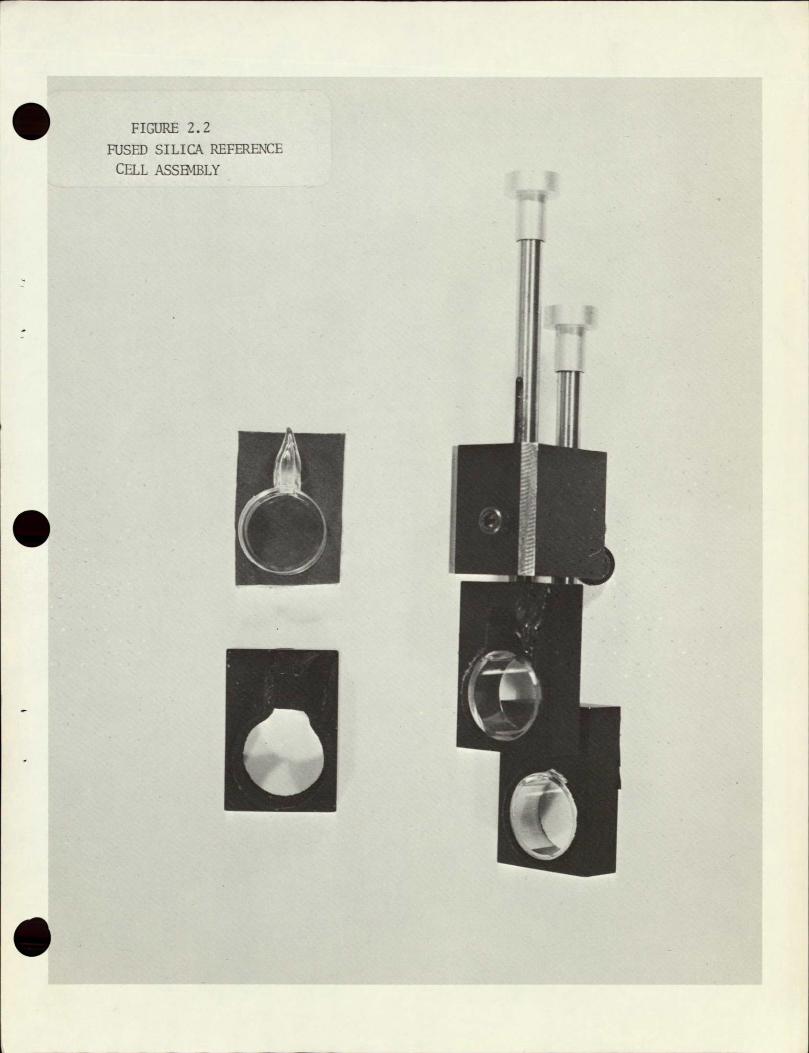

C
IIjI
O l
+
4
1 1
tJII
61
i
-
9 1 eR - c O N f O1 VYi
a3HzN
E W H SE1Y
C
0A
b
2f
i ~ T__ 0z
iT I i-
II _ _ __
IJTI2
h$ TT
- -- ~~~~t - -4 ~2 i
7
- i -
T
FIT R
--
CHARACTER~ISI-A-
~o [Y2
0ODTtLr f
WAVEL mt1m-e-s)
-
10 X 10 TO THE CENTIMETERis x25 cm 46 1513 MASSINU SA
KEWFFFL INESSER CO
z
m
a --shy
---
q a ---------- -------------------shy
X
U3 E-
2-0 q q q m
q w m 1 Hl I
------- ---ZZZ
a
-------qXT rr as
+
15 a
1150
m 1100
L 0 pi 1050
T 1 000
------ --- ------shy 950 0 5
900
850
so 100 200 300 400 500 FIGURE 28 rAP PT TPT)PNT PI)M MPTPPq
0
X0 X 1O0TOTHE CENTIMETER 46 1513 HO lo X 25 CMMACIU
KCUFPEL amp ESSER CO
0
I-t
2 --shy
- - --- ---------8
a 750
850
00
A
255r5 0 0 3040 M---hR
----
---------------N -shy 1
5
------ --
OX 1O TO THE CENTIMETER 46 1513 IoS X 25 CMMltI il
KEUFFEL 0 ESSER CO
14
12
gt10
02
0
0Z
0
00 GA$ ]3UPDU N JWM-II3TflRS PGI
KESE
MI-LO
GARIT
HMIC
358-8
1
4 C
YCL-
ES X
70
tts
ton
s
AO
R
SS
P
nHQ0
I~
~~
I
ifi
II
I II
11
tHi
I
Ill
till
I Ii
i
l l
poio
11
IIij
CII
IIti
l I
I
111O
1
i I
i
IilH
ill
II
m1
111
iii
[I111
II
11
CD
-~
h-
t i
l l
-----
m
11
IN
C H
I
Section 3
FLIGHT RESULTS
31 Los Angeles N320 2 Survey
The results of this survey have been reported on previousiyLlJ Very briefly the most significant features of the Los Angeles program were the close agreement between airborne and ground level (APCD)measurements with respect to synoptic distributions Inparticular for N02 direct comparisons of the two sets of measurements showed the airborne (average) result to be about 13 the APCD value which appears very reasonable considering the great differences inthe two methods
32 i12tjigtTests Coast of Maine (Aug l0-13th68)
A total of six flights were accomplished during which 12 detection was attempted These include the ferry flights into and out of the New England area and an initial exploratory flight along the Massachussetts - New Hampshire coast The ferry flights were non-productive of useful data because of weather conditions and the flight along the New Hampshire coast failed to show detectable levels of 12 The three flights described herein showed significant and consistent Iresponses indicating a build-up of atmospheric iodine with maximum levels indicated in the rvijty of the )atinicus Islands off the Maine coast These flights are summarized in Tables 31 to 33 and illustrated inFigures 31 to 33
Before discussing the results it is worthwhile to briefly consider some aspects of the iodine detection problem Firstly the coast of Maine was selected as a test site because of the abundance of kelp and rockweed which grows inprofusion along the coast between the high water mark on shore and over the ocean floor out to depths of several hundred feet The concentrations of free iodine vapors produced by marine plant isnot known but with a spectrometer noise level of 5 ppm-meters and an effective path length of say5000 meters average concentrations as low
9
12 TRAVERSES - SUMMARY
FLIGHT s
TABLE 31
TIME EDT RUNLINE DIR -ALT (ft) moDE RESULTS
1213 11 S-N 3500 SIDE-LOOK No sionificant chane ir h~rkarrr- 1227 level
1233 21 N-S 2500 SIDELOOK Increase of 13 -nrmreterc -_Fro Tr 1254 Isle to Matinicus
-TAKE-OFF HANSCOMB FIELD 1112 AM EDT TEWP - 18 0C ALTIMETER SETTING 2989Hg WIND - LIGHT AND VARIABLE AT 00( by observation)
LAND - 144 PM hLDT
10
12 RAVERSES SUMvARY FLIGHT 4-
TABLE 32
TIME RUILINE DIR ALT (ft) MODE RESULTS -
EDT -837 11 S-N 2500 LOOKDOWN 30 ppm meters increase from Monhegan-Long-Isle - 9t07 shy
910 21 N-S 1000 SIDELOOK Rise of 10 ppm meters Long Isle to atinicus -927 -
Decrease of 20 ppm meters Matinicus to Ibnhegan
919-94 32 S-N 1000 SIDELOOK No signifant change949-10 43 N-S 500 SIDELOOK Rise of 13 ppm meters from Long Isle to Matinicu
Rock 1007-1021 54 S-N 500 SIDELOOK Rise of 16 ppm meters from Monhegan to 2 miles
- NE of Matinicus (floating seaweed) -shy
1025-10 0 62 N-S 500 SIDELCOK No significant change thugh background S ppn meters higher in vicinity of floating weed
1042-10 6 72 S-N 500 SIDELOOK - sifiai-4change--i -p
1050-11 2 85 N-S 500 SIDELOOK Decrease of 26 ppm mretersfrom just NK of SMatinicus to Monhegan
TAKE-OFF PORTLAND 82_7AM EDT
PRESS 2996 Hg
TBMP 650 F
WIND 2800 Approx
LAND 1120 AM EDT
f
2 TRAVERSES - SUMMARY FLIGHT 5
TABLE 33
TIME RUNLINI DIR ALT MODE RESULTS
EDT 326-333 11 INBOUND 2500 3IDELOOK No significant change - shy
-21 OUTBOUND 2500 IDELOOK 17 ppm meters increase from 4
milesshy - West of Portland to Lightship
3-37-346 31 INBOUND 2500 SIDELOK 14 ppm meters decrease from Lightshipto South Windham -
WIND - - 280
352-444 41 OUTBOUND 3500 SIDELOOK 14 ppm meters in increase from West End of traverse to Lightship
415-427 52 INBOUND 2500 SIDELOOK 12 ppm meters decrease from 8 miles SW- - of Monhegan to Lisbon Falls
445-501 63 OUTBOUND 2500 SIDELOOK 23 ppm meters increase from Augusta to Matinicus
502-520 74 INBOUND 2500 SIDELOOK 95 ppm meters decrease from Matinicus to Small Pt Beach
TAKE-OFF - 259 PM - EDT-PORTLAND
PRESSURE WIND -j16mph 280 LANDING - 540 PM EDT
12
as several parts per billion could be detected With the present spectrometer configuration however the measurement of absolute levels isnot possible because of errors induced by changes in the spectral distribution of incident radiation It istherefore not possible to zero the instrument against an 1 free radiation source such as a lamp or the overhead sky Por purposes of this series of flight tests therefore the procedure was to fly at low altitude with the spectrometer shy
looking sideways and the line of sight tilted down about 10 below the horizontal In this way the effect of spectral changes isminimized and the effective path length is maximized
By appropriate choice of flight lines itis then possible to detect changes in total 12 burden as scanned by the airborne system with a resolution of 5-10 ppmshymeters Sensitivity of the spectrometer was measured periodically by inserting a calibrated reference cell temporarily into the optical path of the instrument
The method used to search for 12 in flight was then to run a continuous profile of the spectrometer output signal over the full length of a traverse with the spectrometer in the side looking mode (except for Flight 4Run 1 when the vertical mode was used) and then to later analyze the trace for significant anomalies or trends The location and direction of each traverse was so chosen as to reveal differences between expected low and relatively high levels of I A brief discussion of each flight follows
Flight 3 Table 31 Figure 31
The northbound traverse showed a very constant background level indicating no substantial difference intotal 12 within view of the starboard looking spectrcmeter over the length of the run On the southbound leg however the trace indicated a steady build-up of I21 reaching a peak in the vicinity of Matinicus Island and then falling off to a level of 16 ppm-meters lower at Monhegan Island Note that only changes in signal level which occur over the duration of any one traverse are significant A comparison of absolute levels between any two traverses isnot valid
- 13
because of possible differencesinspectral gradients as previously explained
Flight 4Table 32 Figure 32
Note that the first run of this flight was made with the spectrometer in the
vertical or lookbdown mode In this case as on ether occasions when the vertical
mode was attempted the background fluctuation was relatively high A portion of the strip chart recording from this run is shown In Figure 34 Cc)
The purpose of flying traverses on either side of Vtinicus Isle was to determine
if it was possible to break out the atinicus group as a distinctive 12 anomaly
Figure 32 shows the flight lines and the traverses or irung during which significant changes in 12 level were observed The first run using a vertical look shows the
12 level inthe vicinity of Long Isle to be 30 ppm-metershigher than 12 levels
around Monhegan On the second run using the side-lookmode the background level
tended to rise slightly from Long Isle to Matinicus (10 pr-meters) but showed a
definite drop (20 ppm-meters) from Matinicus to Monhegan The same trend in12 levels was observed on runs 45 and 8 Note that no significant changes were noted on runs 36 and 7 indicating either that no significant quantity was observed
or what ismore likely that the Ivapors were so dispersed as to show no signifishy
cant change in total burden over the duration of the run Note that runs 36 and 7
are all upwind of the Matinicus group
Flight 5 Table 33 Figure 33
The traverses shown in Figure 33 were designed to reveal a coastal 12 anomaly
Note that there is a gradual but consistent build up of 12 off the coast which is independent of aircraft heading The absence of a more abrupt change or a
more distinctive anomaly can be explained by the extremely irregular shoreline
and the gradual transition to a marine atmosphere Unfortunately the traverses
could not be extended out to sea without violating National Defence prohibited
14
air space Ihe first run was spent largely in making instrument adjustments and
the factthat no significant trends in the I levels was noted is not too significant
A typical example of the strip chart recording for Flight 5 is shown in figure 34 (a) The chart reads in increasing time from right to left and shows an increase
of 23 ppm-meters in background 12 level from Augusta to Matinicus For an assumed 5000 meter path length this would represent a background 12 level some 5 parts
per billion higher in the vicinity of Matinicus than in the vicinity of Augusta
Determination of Free Iodine amp Total Iodine in Seaweed
Wet chemistry measurements of very low 12 concentrations in the atmosphere are
difficult to make and a comprehensive series of measurements of the scope required
to confirm the remote sensor results would be a major undertaking On the other
hand measurements of the 12 content of seaweed although not as convincing as measurements in the free vapor phase are very much simpler to make For the sake of ground truth then a sample of rockweed was obtained from the rocky coastline
of Maine during the 12 flight program and analyzed in the BRL laboratories The following describes the procedure followed and the results obtained
Free Iodine - A 3 gin sample of seaweed was placed in a U-tube which took the place of the U-tube containing Iodine Pentoxide in a set-up more usually used
for the determination of carbon monoxide in samples of gases
This U-tube has provision for being heated to 160C and was followed by a bubbler
containing 3KI solution The seaweed was heated to 160 0C while being swept with dry C02 free air Any free iodine present would have been vapourized and
absorbed in the KI solution where it could have been determined by titration with N
N indicator solution assumed a brown colouration on running the test no iodine was present
as no blue colour was produced on adding the starch indicator
1000100 sodium arsenite using fresh starch Although the KI
is
From considerations of sensitivity of the method and the amount of seaweed sample taken the minimun detectable level of 12 was calculated and found to be less than 5 ppn-WW This means that iffree 12 was present in the sample it would have to have been less than 5 ppm WW
rotal Iodine
Dver 50 grn of seaweed was initially taken This was ashed completely in a Nickel crucible in the presence of sodium carbonate which combined with the potassium carbonate present in the seaweed ash to give a clear quiescent melt his melt was dissolved in dilute HCL and the resulting solution made to 1Vi
zonc HCLwater
[he iodide was then precipitated as palladous iodid6 with palladous chloride solution following the method on P 493 of Reference (10)
[he precipitate was allowed to stand for 24 hours then filtered through a fine 3intered glass crucible and then washed 4 times with warm water after which it was oven dried 6 1000C for 1 hour
From the weight of Pd 12 obtained and the original weight of seaweed taken a ialue of 0140Ww Total Iodine was obtained (as received)
rom the loss of weight on drying a further sample of seaweed a figure of
01560 WW Total Iodine (Dry Basis) was obtained
- 16 shy
DISCUSSION OF 12 RESULTS
The inprovement in signal-to~noise ratio of the side-look relative to the vertical mode is readily seen in Figure 34 A three second integration time was used for Figure 34 (a) and (b)and one second integration time for Figure 34 (c) Conmaring figures 34 (a) and C) the internal system noise is the same but the background fluctuation or total noise appears to be 2-3 times higher for the vertical mode over the side-look mode
The very substantial offset produced by differences in spectral gradient between sky radiation and radiation reflected from the oceans surface is evident in Figure 34 (c) Proceeding from right to left an offset of 53 ppm-meters was recorded when switching from sky to water The reason for this offset as mentioned earlier is inherent in the instrument mechanization and is explained fully in Appendix I The new instrument design proposed in Secti6n 4 should overcome this deficiency or at least greatly reduce it
Figures 34 and 36 are 35 mm photographs taken from Aero-Comnander Figure 35 shows Matinicus Rock the most seaward member of the Matinicus group The visible
rockweed growth along the shore is typical of most of the rugged Maine coastline
Figure 36 shows seaweed floating freely on the oceans surface in the vicinity of the Patinicus Islands Many such sightins were made during the course of the program
The laboratory analysis -of the seaweed sample confirmed the presence of a significant concentration of total 12 in the plant but free 12 was undetected The absence of free 12 is not surprising since the weed sample was stored in unsealed containers in a semi-dehydrated state for several months before analysis could be made This is more than enough time to permit the escape of any free 12 originally stored in the plant
The following points may be used to summarize the findings of the 12 flights () Data runs consistently showed higher levels of atmospheric 12
along the coast than further inland
17 shy
(Z) On the days of flights the 12 levels inthe vicinity of IMtinicus Isle
appeared to be significantly higher ina relative sense than I levels
elsewhere along the coast
33 QATCOGA NO92S02 SURVEY
Synoptic distributions and plume chases for NO2 and a plume chase for S02 were conducted inthe Chattanooga area on behalf of the National Air Pollution Control
Administration (NAPCA) in the period August 3rd to August 7th The results of
the survey are reportedin reference (2) It is useful however to discuss here certain aspects of the Chattanooga data namely instrument and background noise levels Moreover it is preferable to usd these data rather than the Los Angeles
data for this purpose because of improvments made to the equipment following the Los Angeles program (see Section 2) Two of the most significant improvements
from noise stand-point were (a)more effective vibration isolation of the mirror
system and (b)improved light baffling within the aircraft mounting fixture These modifications resulted ina-marked improvement in system stability and measurement
repeatability The system performance as demonstrated inall subsequent flights represents the true capabilities of the correlation spectrometer at its present level
of development
Figures 37 and 38 illustrate typical noise characteristics of the N 2 and So2
channels respectively Note that the minimum detectable signal inboth channels
is limited by two very different types of noise namely (11 internal instrument noise which is a combination of photon noise and synchronous detector noise and
(2)external noise which is a complex function of many variables in the total measurements The most significant component of external noise isbelieved to be
both short and relatively long term variations in spectral distribution or gradient
This is discussed further in Section 37 From Figures 37 and 38 it is apparent
that internal noise isabout 8 ppm-meters for NO2 and 10-15 ppm-meters for SO2 The external noise is the slow irregular signal fluctuations For NO2 over varied tree and brush covered terrain with water patches and cultured or builtshy
up areas the external noise isapproximately 15 ppm-meters and for SO2 about 20 ppm-meters Both of these values are for an aircraft altitude of 8000 ft
External noise tends to decrease with increasing aircraft altitude
- is shy
34 PLUME CHASE EPERIMENTS
A plume chase is a series of airborne measurements of effluent from a conshy
centrated source of emissions sfach as-ofi or Xiamp_amp chimneys or stacks at various
The primary purpose of the plume chase experimentdistances from the stack exit(s)
the accuiacy of the remote sensing techniqueis to provide data which will permit
to be determined It is the simplest and perhaps the most accurate way of comparing
the remote sensing method quantitatively with other established and proven methods
The plume parameter of first interest here is the mass flow rate
A successful plume chase experiment requires a rather stringent set of plume and
environmental conditions namely
(1) A straight horizontal plume with a low dispersion or spread angie
(2) Adequate clearance between the plume and ground for aircraft flight
(3) Absence of competing sources of emission
(4) Flat and uniform topography under the plume
(5) Absence of low cloud cover
(6) Adequate solar illumination
(7) No low level (legal) flight restrictions
The geography of the Toronto area water-front offers many of the above noted
Lake Ontario provides a strong positive influence for the stableprerequisites
air conditions required for an undisturbed plume a singularly potent source of
Lakeview Generating Station with noemissions is available at the Ontario Hydro
competing sources downwind from it (assuming a westerly wind) and there are no
low level flight constraints over the lake surface Unfortunately during the last
two months of this experimental program (October and November) adverse weather
conditions severly restricted the opportunities for plume chase experiments Low
lying cloud is particularly objectionable for a precise test of this kind since it
but it also promotes instability and may not only restrict the view of the plume and the groundconvective mixing in the layer of air between it
19
The first flight results discussed below (August-2768) was actually conducted
under NAPCA contract o PH22-68-44 but are presented here because of their pershy
tinence
August 2768 NO2 Plume Chase
Figure 39 shows the plume outline and the aircraft flight lines for a series of
NO2 measurements of the effluent from Lakeview Generating Station A photo of
the Generating Station from a previous flight is shown in Figure 310 Wet
chemistry measurements were made at the source simultaneous with the airborne
measurements Figure 311 shows the actual strip chart profiles of two traverses
over the plume and Table 34 lists the data obtained Figure 312 illustrates in
a simplified form all plume profiles obtained All traverses of the plume were
made above the plume and at right angles to the plume center line at an aircraft
altitude of 1525 meters (5000 ft) The build up of NO2 with distance or time2 is evident A peak value of 76800 ppm-m was obtained at 16 Kilometers from the
source Mass flow may be found as follows
m factoorMass flow = Plume Cross Section (ppm-m2) Xi__ 1 x windwnrveotvelocity
x gas density (gmsm) x 106
Plume Cross Section = 76800ppm-m2
Wind velocity = 671 to 940 meterssec
NO2 gas density = 195 gusliter 700F and 1 atm
(single molecule) m factor = 249 from NO2 atmospheric model for 4V
latitude Aug 28th solar zenith angle- 41
3 1 then mass flow =768 x 10 x (671 to 940) x 195
x 10 x 106 403 to 565 gmssec-
161 to 225 tonshr
- 20 shy
PLUME CHASE DATA - LAKEVIEW GENERATING STATION - AUGUST 27 1968
TRAVERSE DISTANCE PROFILE HORIZONTAL PROFILE PROFILE PLIM CROSS NO FROM LENGTH SCALE AREA HEIGHT SECTION
SOURCE (KM) (cm)
(meters) (cm2)
(AVERAGE) (CM)
2 (ppm-m 2)
1 08 11 287 24 218 5350
2 32 30 287 50 167 11150
3 56 81 287 108 134 24100
4 80 57 287 140 246 31200
5 105 84 287 270 321 60200
6 129 95 287 305 321 68000
7 153 116 287 344 297 - 76800
8 177 92 287 342 372 76200
9 129 87 296 210 41 48300
10 80 48 290 62 12914000
11 32 48 290 63 131 14200
Vertical Scale (All Traverses) = 777 ppm-mcm
PlLme Cross Section
= Profile Area x Vertical Scale x Horizontal Scale
= 24 x 777 x 287
= 5350 ppm-M2
TABLE 34
21
The assumption is made in the above calculation that the plume is sufficiently
wide in the area of the measurement (3330 meters) that the atmospheric model
(whichassumes a distributed homogenous gas layer) isvalid If this assumption
is not entirely correct then the above answer would tend to be lower than the actual
value
Ground Truth at Lakeview GS
Ground truth measurements were made at the base of one of four stacks of the
Lakeview Generating Station using the Phenol Disulphonic Acid method Commenceshy
ment of airborne and ground measurements was co-ordinated by preflight briefing and
visual signals from the aircraft at the start of the first traverse The method
of determining No2 concentration and therefore total amount of N02 emitted in
stack gases is as follows
The NO2 concentration is obtained by allowing a known value of stack gas to
enter an evacuated glass flask containing an acid-peroxide absorbing solution
After allowing 24 hours for absorption to reach completion the NO2 and potential
NO2 (eg NO) ispresent in the absorbing solution as Nitric Acid This is
neutralized with caustic soda solution and the absorbing solution now containing
the NO2 and NO as sodium nitrate is compared colourimetrically with known potassium
nitrate standards by means of the absorption at 4200 A of the phenol disulphonic
acidnitrate complex formed with the sodium nitrate or potassium nitrate standards
The absolute amount of NO2 and potential NO2 presents in the stack gases is calshy
culated from the ppm vv concentration readily obtained from the above coulorimeshy
tric method and the total gaseous emission from the various stacks
In the case of Lakeview Generating Station this emission is calculated from figures
kindly supplied by Ontario Hydro giving the ibshi of air fed to the generator
units and the tonshr of coal fed to the units together with a complete analysis
22
of an average sample of the fuel they use From these figures it is possible to
calculate the total emission of gases from the power station assuming the nnber
of units on stream is known and the excess air utilized is known
For the August 27th flight a total of four samples were drawn at the source with
the following results
SAMPLE CONCENTRATION
(1) 190
(2) 180 Average 192 ppm (3) 215
(4) -185
Basis for Calculation of Output of NO2 from Lakeview Power Station
Lakeview Power Station give an optimum rate of coal-burning (per unit) of
100 TPH (Tons Per Hour) which yields theoretically 28 x 106 lbshr of total
effluent On the 27th of August 1968 3763 TPH of coal were being burnt throughshy
out the power station This would yield 1054 x 106 lbs per hour of total effluent
of which 192 ppm volumevolume is oxides of nitrogen which converts eventuallyVw
to Nitrogen Dioxide The figure of 192 ppm Vv can be converted to a W value
by multiplying by the ratio of the densities of NO2 and flue gas ie X 23
giving 294 ppm weightweight potential NO2 in the total flue gases
This gives a figure of 155 Tons Per Hour total potential N 2 emitted on 27868
From the actual Power Station output over the hour of the analyses which was 125
up over the hourly average for the day an extra 125 of coal may be assumed to
have been burnt and an extra 125 of potential N02 produced This gives a final
figure of 175 tons for the hour inquestion
It may be said as a confirmation of the accuracy of the effluent figures provided
23
by Lakeview Power Station that a calculation of theoretical SO emission yields 2
1335 ppm v based on one coal aalysis exhess air fed to the furnaces and assuming i0l conversion of Sulphur in the coal to S02 Our all-time average for ppm vv S02 is1425 ppm
September 2768 NO2 Plume Profiles
The ground track or flight lines and the plume outline are shown on the map of Figure 313 The purpose of this flight was to obtain remote measurements of mass flow from both above and below the plume and to compare both sets of measurements with measurements taken at the sburce using standard wet chemistry methods- Figure 314 shows the actual strip chart profiles of two traverses (inshycluding additional plume from another refinery) and Table 35 lists all data obtained
24
Figure 315 illustrates in a simplified forn theprofiles obtned for all passes over and under the plume The aircraft altitude for the overpass was 457 meters msl for all three lines and was estimated to be 30 40 meters above the plume at the plumes highest point ie at the 8050 meter traverse The aircraft altitude
for the underpass for all lines was 138 meters msl which was about 55 meters above the lake surface With a light (4mph) wind the comibined plume from the reshy
fineries numerous emitting sources was quite irregular in shape and resulted in conshy
considerable variation on plume cross section from one pass to the next (at a given
range) as shown inFigure 315 The irregular shape of the plume is also evident
in the photograph taken of the plume and the source following the last traverse Note also inFigure 315 that the plume cross section (profile area) has minimum value
close to the stack and maximum value at a distance of 4830 meters (5miles) from
the source indicating that under the conditions prevailing at the time the build up of NO2 that is the oxidation inthe atmosphere of stack NO emissions was largely complete in the distance of about 5000 meters downwind or about 45 minutes after emission The significant reduction in cross section from 4830 meters to
8050 meters downwind indicates that NO2 isbeing lost from the plume by diffusion
andorsubsequent reactions in the atmosphere Note also from Figure 315 that the plume cross sections from above the plume tend to be larger than cross sections
obtained from below the plume This is to be expeicted since the radiation source used in the normal look-down mode is the total sky while in the look-up mode
it is only a resolution element of the sky directly above the aircraft A comparishy
son of the look-down to look-up profiles yields a plume m factor similar inmeaning
to the m factor of a distributed gas layer but peculiar to the plume geometry and sky conditions which existed at the time of the measurement Because of the lumpy
shape of the plume considered here good repeatibility of the measurement is
demonstrated only at the 4830 meter crossing (traverses 456 7) Here the
overpass repeats within 25 and the underpass within 6
The base of the triangle is scaled to the width of the chart profile and the
area is scaled to the integrated area of the plume profile on the chart
25
PLU E DATA - SEPTDMBER 27th 1968 - OIL REFINERY
TRAVERSE TIME OVER PROFILE AVERAGE VERTICAL AVERAGE PLUM NO UNDER AR HEIGHT SCALE BURDEN X SECTION
(a) (Can) (ppmmr) (ppm-rn) ppm-rn12
cm x 1io3
1 1545 0 144 192 294 565 124
2 0 84 205 294 603 725
3 U 26 140 263 105 20 4 160C 0 320 147 166 244 159
5 0 403 190 166 316 196
6- 1615 U 242 235 96 226 68 7 U 257 279 96 268 72 8 -1630 0- 248 180 166 298 120
9 NO DATA
10 U 304 322 96 309 85
11 1650 U 128 158 96 152 36
Profile horizontal scale I cm = 293 meters
TABLE 9Z5
- 26
The mass flo in both cases can be calculated as follos
for traverses 4 5 (over pass)2
profile area = 36 cm average
vert scale = 166 ppm-mca
horiz scale = 293 meterscor
103 2plume x section = 36 x 166 x 293 = 175 x ppm-m average
wind = 179 meterssec (4 mph)
NO2 density = 195 ginsliter 70] Q I atm (single molecule)
m factor = 27 (1400 EST Sept 27th Oz = 52 homogeneous layer
Therefore mass flowI = 175 x 10 x 1 x 179 x 195 x 10 x 1077 shy
= 226 gmissec
- lbhr
Similarly for traverses 67 (under-pass)
2area = 25 cm average
vert scale = 95 ppm-ncm
horiz scale = 293 metersam
Therefore piue x section 25 x 95 x 293
= 696 x 103 ppm-m2 average
x 10 - 6and mass flow = 696 103 x 179 x 149S k 103
= 243 gnsseeshy
= _1 940 l
Of the two results the underpass measurement should-be the most accurate since
uncertainties in m factor are avoided
27
The actual pltme in factor may be found from the ratio of pl-e x sections
3ie plume wfactor 17103 6 x 10
= 251
This value compares very well indeed wiith the theoretical value of 27 used above
The fact that it is less than the theoretical value is to be expected since the plume width is limited and some radiation reachino the snactrometer would have nassed
through the plume only once
Refinery Ground Truth
S mnutaneous with the airborne measurement wet ciiemistry measurement oplusmn total oxides of nitrogen were taken at the primary sources of emissions within the refinery compl ex
Results are as follows
Emitting Source Volume pm vV N flsw O2 ft min ft min
Boiler House 108000 270 30
1 Crude Unit R2 000 80 -4
Heater
CO Boiler 167000 240 40
2Remaindei 23000- 80 19
Total NO2 93
3 Total NO2 from refinery 93 ft min
= 2600 litersnin
= 767 ginssec
= 612 lbhr
- 28 shy
DISCUSSION OF NO PLUME CHASE PESULTS2
Although plume measurements of Lakeview Generating Station check very closely with ground truth values the refinery plume measurements showed a mass flow exshyceeding the ground truth value by a factor of three Although the reason for the lack of closer agreement in the second case is not known at this time the
following factors are probably significant
(1) Lakeview is well defined and well regulated source whereas the refinery
in question is a multitude of sources which are quite variable and difficult
to monitor
(2) Lakeview is an isolated source whereas numerous other industries occupying the shoreline near the refinery making it difficult to discriminate between
plumes The proximity of other industrial sources is evident in Figure 316
- 29
35 DESCENT PROFILES
The term ascent descent or vertical profile is used herein to describe a conshytinuous chart recording or plot of spectrometer output as a function of airshycraft altitude The purpose of this experiment is to test the validity of the computerized radiation transfer equations and the atmospheric model The preferred meteorlogical and flight conditions for this experiment are as follows
(1) A single well defined inversion layer with a substantial concentration
of pollutant uniformily distributed in the mixing layer ie in the layer of air between the inversion and the ground
(2) minimal cloud cover (3) smooth unidirectional low spded wfnd
(4) well defined identification points on the ground
(5) no low level flight restrictions
(6) adequate light
The flight procedure is to fly the aircraft along a horizontal straight line
course betiqeen two well defined points in space -first in one direction with the spectrometer looking at the sky above the aircraft and then in the opposite direction with the spectrometer looking at the ground below the aircraft This
is repeated at 2-3 thousand foot intervals from a maximum altitude of 11000 ft to the minimum altitude consistent with flight safety
The Lake Ontario air space again provides many of the desired features for this experiment Prominent shoreline features make excellent identification points and dense population centers provide adequate pollution levels for all wind direcshytions with the exception of easterlies between 060 to 120
A total of four flights were accomplished three NO2 descents and one SO2 deshy
scent One NO2 descent was performed over Lake Simcoe (50 miles North of Toronto) because of good meteorlogical conditions in the area and visibly dense cloud
30
of pollution produced by the Toronto area and south easterly winds Each flight is discussed in detail below
MO2 Descent over Lake Simcoe Sept 1768
Figure 317 shows the flight line Figure 318 Ca) shows the change in NO2 channel
response in volts as a function of altitude and is a plot of the total signal data
column of Table 36 At each altitude the calibration cell was used to obtain the incremental sensitivity and scale factor which was then used to convert the change in total signal to equivalent gas burden Note that the total signal
voltage and hence the total equivalent burden is normalized to the last traverse at the lowest altitude flown in the look-up mode ie Run 12 of Table 36 The
plotted data of Figures 318 (b) and 319 are therefore only relative ie they
show only the difference in spectrometer output between the reading taken at a
-iven altitude and the reading obtained at the last traverse
-As noted in Figure 31g and indicated in Figures 318 (a) and 318 (b) tmy stable
inversion layers were observed from the aircraft These are usually noted in flight during an initial ascent and altitude readings taken when co-altitude with the top of the haze When the top of the haze is well defined its altitude can be
judged with a reaptability of + 200 ft
When descending through a gas layer to which the instnmxent is sensitive the instrument output can be expected to fall as the total effective optical pathshy
length (aircraft to ground to top of layer) is reduced As can be seen in Figure
318 (a) and 318 (Is)this is indeed the case in fact there is significant fall off in signal before the upper hate layer was reached indicating that some gas
was present above this level
Referring now to the look-up mode as the aircraft descended down through the layer
31
NO2 DESCEANT DATA LAKE SIMCOE - September 17 1968
RUN AC TIME LOOK SIGNAL SIGNAL SIGNAL VERT SENSITIVITY TOTAL NO ALT EDT UPDOWN OFFSET RIG TOTAL SCALE EQUIVALENT
(My)MSL (TV) wm) Cppm-m BURDEN (ft) (2) (4) -rJ(3) ppm0n)-m
1 11000 1610 U 420 420 -90 518 65 154 337 2 D 700 140 848 66 151 560
3 9000 1620 D 700 01 708 66 1551 467 4 U 700 48 755 66 151 498 5 7000 U41635 U D A A NO G-OOD 6 5000 16-r0 D 560 10 578- 47 213 272
7 U 700 0 708gt 4 213 333
S 3000 17DS D 280 35ft 3 45 222 145 9 4 U 280 30 2318 45- 212 - 143
10 1000 1720 D 140 42 190 37 270 70 11 U 0 34 42 37 - 270 16 12 U 80 -8 0 2702 00 37 0
I
Notes (1) Averagetime of traverse (2) Offset voltag(rte( drto maintain trace on chart Relative to an assigned offse
voltage of zero or run 12 (3) Measured from zero grid line on strip chart (4) These values representa change inthe sum of the offset voltageand the chart
reading from an assigned total siknal of zera forfrun 12shy(5) Relative to an assigned total equ valent ouraen of zero or run 12
TABLB53
rn2 DESCENT DATA - IAKE QTNJM OFF NIAGARA October 2 1968
RUN AC TIME LOOK SIGNAL SIGNAL SIGNAL VERT SENSITIVITY TOTAL NO ALT EDT UPDOWN OFFSET RDG TOTAL SCALE ) QUIVALENTMS y) (my) mv) 4m BURDEN
(ft) (2) (3) C4) pmU-r (ppm-m)
I U 5q0 200 660 45 222 297
2 D 500 100 560 42 38 - 235
3 000 1150 U 5d0 240 700 47 213 315
4 D 500 140 600 38 262 228 S 7600 1220 b 5Q0 27Q 730 45 2-22 328
6 D 500 80 540 38 2 62 205
7 5000 1250 U 5Q0 170 630 40 250 22 8 D 500 40 500 40 250 200
9 3000 1320 U 0 180 140 39gt 256 545
10 D 0 40 0 3sect 256 0
)
) I
Notes (1) Average timb of traverse (2) Offset voltagereqdto maintain trace on chart Relative to anassigned ofset
voltage of zero for run 12 (3) Measured from zero grid line onstrip chart (4) These values represent a change in the sum of the offset voltage and the chartreading from an assigned total signal of zern for run 12 (5) Relative to anassigned total equivalent buraen of zero Por run 12
TABLE37
NO2 DESCENTDATA - LAKE c O OFNIAGARA October 16 1968
RUN AC TIME LOOK SIGNAL SIGNAL- SIGNAL VERT SENSITIVITY TOTAL NO ALT EDT UPDOWN OFFSET RDG TOTAL SCALE 3QUIVALENT
MS L (ft)
(my)(2)
(My) (3)
(m)rmlgtt C4)
BURE (ppm-M)
(5) 1 9Q00 1624 U +500 500 900 21 475 189 2 1628 U V 600 1000 21 475 210 3 1633 D - 300 700 23 432 161
4 1640 D 350 750 23 432 173
5 7000 1650 U 650 050 21 475 220 6 111656 aB 300 700 21 475 147 7 5000 1704 U i 600 1000 19 525 190 8 1710 D 225 625 19 525 119 9 3000 1718 U 525 925 20 50 185
10 1724 D 1100 5001 9 525 95 11 1000 1732 U 375 775 20 50 155 12 1738 D 0 190 90 21 475 19
13K 500 1743 U 0 400 300 19 525 57
14 1749 U 0- 425 325 19 525 62
15 1754 D 00 100 0 21 475 0 16 h 1759 D 0 150 50 21 475 10
Notes (1) Average time of traverse C2) Offset voltage re6dto maintain trace on chart Relative to an assigned offset
voltage of zero for run 12 (3) Measured from zero grid line on strip chart (4) These values represent a change in the sum of the offset voltageand the chart
reading from an assigned total signal of zerQ forfrun 12 (5) Relative td an assigned toltal equivalent Durcien o zero Eor run 12
TABLE 38
SO2 DESCENT DATA - LAKE ONTARIO OFF HAMILTON Not-ember 4 i968
RUN NO
AC ALT MSL (ft)
TIME EDT
(1)
LOOK UPDOWN
SIGNAL -OFFSET (i) C2)
SIGNAL RDG (mv) (3)
SIGNAL TOTAL Cmv) C4)
VERT SCALE
ppm-
SENSITIVITY QUIVALENT
ppm-r
TOTAL
BURDEN (mUrn)(4)
1 90Q0 1220 U 0 225 1025 35 285 359
2 U 0 260 1060 39 256 413 3 D 0 720 1520 31 322 471 4 D 0 675 1475 31 322 457
5 7000 1235 D 0 600 1400 28 356 392 6 U 500 150 -450 44 227- 202
7 5000 1245 D 0 400 1200 39- 256 468 8 U -500 100 400 39 256 156 9 Df 0 440 1240 39 256 484
10 11
3000
1255 U D
700 0
250 -500
350 1300
305 31
-327 322
107 403
12 1000 1315 U 700 400 500 34 290 173 13 D 0 800 1600 22 452 352
14 - U 700 350 450 31 322 140 15 D 0 600 1400 375 266 525 16 9000 -1335 U 400 300 700 34 295 238 17 D 0 400 1200 375 266 450
Ntes (1) Average time of traverse (2) Offset voltage reqdto maintain trace on chart (3) Measured from zero grid line on strip chart (4) These values are not absolute and represent oily-a change in
response as a function of altitude
TABLE 39
one would expect to see a monotonic increase in total gas within the view df the instrument Referring to Figures 318 (a) and 318 Cb) however it can be seen that an increase was recorded only down to the highest haze layer and desshycending further produced an apparent reduction in the total number of molecules seen by the instrument Since this is obviously an impossibility additional flights were made for NO2 on Oct 2 and Oct 16 1968 As shown in Figures 321 and 324the look-up profiles consistently show little change or a slight increase in look-up signal dowa to the inversion layer and then very definite negative tenshydencies below this level This behaviour can be explained in terms of instrument mechanization As shown in Appendix I the spectrometer response not only to the absorption characteristics of the gas it is programed for but also to changes in spectral distribution of the radiation source In the aircraft of course the look-up radiation source is the sky whose spectral characteristics depend on both sun angle and the scattering characteristics of the atmosphere For a given sun angle scattering characteristics depend on particle size and number distribushytion which are quite variable in the lower levels of the atmosphere and particularly so at the top of a haze layer In the foregoing Figures the negative going NO2 channel signal is the net result of two responses namely a positive going NOZ
absorption signal and a negative going spectral gradient signal of which the latter predominates Above the haze layers the response is predominantly NO absorption Figure 319 shows graphs of the photomultiplier WM) voltage and sensor sensitivity plotted -against altitude The curve of EM voltage which is an inverse function of light level shows a significant low point right atthe strong inversion altitude of S000 ft msl This means that the light intensity looking up into the haze layer from immediately below it was higher than at any other point in the descent This would be due to enhanced long wavelength contributions from large particle and aerosol scatterers in the haze layer
The change in instrument sensitivity shows a definite tendency to increase below the inversion in the look-up mode This is due to a general levelling of the spectral distribution due again to enhancement of the long wavelength contributions
- 32 shy
It is -worth noting here that the gradient error evident in the look-up data will be present to a much lesser extent in the look-down mode because the radiation source includes direct radiation from the sun (via the earths surface) and therefore the affect of shifts in energy disttfbution in Backscatter from haze will be less pronounced
NO2 Descent over Lake Ontario October 268
This flight was discontinued after descending to the 3000 ft level because of weather The data however is quite good nd confinnt the results of the Lake Simcoe flight as mentioned earlier
NO2 Descent over lake Ontario October 1668
This flight was carried out under extremely godd conditions The results are essentially the same as for previous flights with the exception of a low haze layer at about 700 ft msl A photograph of this low layer isshown inFigure 326 Unfortumately the aircraft was not really co-altitude with the top of this haze and the interface is not as clear as the visual observation A dashed line approximates the haze top
- 33 shy
so2 Descent Over Lake Ontario - November 4 1968
Figure 327 shows the flight line and as indicated by the iWind arrows the
descent was made through pollution carried by a north east wind The spectroshy
meter millivolt output is shown plotted against ac altitude in Figure 328 and
the same output in terms of ppm-meters is presented in Figure 329 Note in
Figure 329 that the change in apparent gas burden changes sign several times
during the descent indicating that the gradient component of signal is at least
as large as the true SO2 signal and can be positive or negative relative to the
so2 absorption signal
The effect of changes in spectral gradient or instrument sensitivity is evident
in Figure 330 Although the number of data points on any one profile is
rather limited there is nevertheless a strong correlation between the locations
of the points of inflection on the look-down sensitivity curve and the layers of
stable air in the atmosphere During the descent temperature readings of
ambient air were taken using the aircraft thermometer which has a feadout reshy
solution of 10 C These data are shown plotted in the lower curve with the
stratified layers of stable air shown by shaded areas Stable layers of air are
indicated by temperature gradients less than the dry adiabatic lapsd rate ie
less than a fall of about 1degC for every 500 ft increase in altitude
- KA shy
37 GENERAL CCNMENTS ON FLIGHT RESULTS
The foregoing flight results including NAPCA Chattanooga work reference (1)confirm the results of the previous contract NAS9- 72 42 in terms of feasibility of the remote detection of SO2 and also clearly establish the feasibility of remote detection of atmospheric NO2 and 12 Quantitatively more ground truth data has been gathered for 102 than for SO2 and good ground truth comparisons for 12 have yet to be accomplished The most useful and most accurate ground truth data to date in so far as proving the remote sensor is concerned have been the NON02 stack measurements In general the comparisons of airborne - ground level measurements of NO in Los Angeles and Toronto plus preliminary results of2
Chattanooga (NAPCA is currently finalizing the Chattanooga data analysis) are so encouraging that no changes to the N02 atmospheric model are contemplated at least until the results of more precise experiments are available The SO2 airborne-ground level comparisons on the other hand consistently indicate that airborne results tend to be higher than the actual Apart from the spectral gradient problems discussed below a contributing factor to the apparent error may lie in the values assigned to the SO2 absorption coefficients used in the
so2 atmospheric model Theoretical work is presently underway to obtain more precise values and these findings will then be used along with more accurate comshyparisons with ground emissions to refine the model
The generation of accurate Iodine ground truth data promises to be perhaps the easiest gas to handle so far It appears quite feasible to set up an experimental
I2 vapor generator with sufficient strength to serve as an effective calibrated source For example a 50 ppm-meter response of S second duration could be obtained from a plume with a source strength of 35 gmssec (50 lbminute) in a 5 metersec (11 mph) wind Such a facility could comprise a battery of truckshymounted hot air blowers exhausting into the atmosphere through high capacity 12 evaporators A mobile test site of this kind could be readily set up for example on the shores of Lake Ontario and the plume chased in the conventional manner
- 35 shy
Perhaps the most significant feature of the test results is the magnitude of the
error in the measurement caused by changes in spectral distribution Insufficient data were available from the original feasibility flights to reveal this error
and in fact it was not until after the final series of equipment modifications
(following the Los Angeles work in May of 1968) that this type of error became clearly identifiable This was subsequently confirmed by the theoretical treatshy
ment given in Appendix I and the N02 and SO2 descent experiments It is important
to note here that this type of error has not had a substantial effect on relative
measurements of gas clouds in the look-down mode In other words in plume chasing
experiments where the plume contribution is measured relative to the background polshylution eg the Toronto plume chases the apparent accuracy of the measurement has been most encouraging It is when attempting to measure the absolute level of polshy
lution in the atmosphere using the sky as a zero reference that the spectral gradient
error has a significant effect on the accuracy of the result Furthermore this type
of error is largest in the ultra-violet (SO2) mode and least in the blue=visible
(NO) mode The unexpectedly high S02 levels found in the Washington DC and Los
Angeles surveys may be due in part to the presence of spectral gradient errors in the
measurement There is also good reason to believe that a large part of the background
fluctuations present in the synoptic profiles of all three gases is due to spectral
gradient noise components These will be induced not only by variable atmospheric
scattering but also by the spectral characteristics of the terrain As shown by
Figures 37 and 38_ the nature of the terrain has little affect on background noise in the SO2 and NO2 modes but is quite pronounced in the 12 n5de as shown
in Figure 34 This is so because the wavelength dependency of the reflectance
properties of most terrain materials in the middle near ultra-violet is not strong
as shown in reference (3) but is quite pronounced in the visible as shown in reference
(4) The relatively high background noise level in the S02 mode then can be atshy
tributed mainly to a fluctuating gradient of the ground-reflected radiation caused
by atmospheric effects plus no doubt a noise contribution from the SO2 concentration
pathlength product
- 36 shy
The NO2 m6de of operation appears to be the least affected by gradient errors due to either terrain or atmospheric effects
Unwanted scattered radiation from the pollution layers in the atmosphere may not only modify the spectral disttibution of radiation reaching the instrument but it may also enhance or dilute the spectral signature The presence of backshyscattered radiation from the pollution layer is evident in the NO2 descents of Figures 319 322 and 325 and in the SO2 descent of Figures 330 Since the sensor AGC system maintains a constant output level from the photomultiplier by automatically adjusting the PM tube voltage an increase in voltage indicates a reduction of radiation received Note that in the look-down mode as the airshycraft descended there was little change in PM voltage until passing through the haze layers after which there was a gradual but steady increase ie a gradual decrease in total radiation received within the spectral bandwidth This indicates that back scattered radiation was coming from particles fairly uniformily distributed in the layer although Figure 325 indicates that a partishycularly dense layer of scatterers occured below the lowest inversion at 700 ft
In the normal look-down mode the effect of babkscattered radiation from aerosol and particulate matter in the atmosphere on the accuracy of the measurement will depend on the spatial distribution or location of the aerosol particles relative to the gas If completely above the aerosol then the gas signature will not be afshyfected and if it is completely below the aerosol then the effect of dilution will be maximum Undoubtedly in the actual case the answer lies somewhere beshy
tween these two extremes
Techniques are now being considered which will enable the aerosol backscattering effect to be estimated and allowed for in computing gas burdens in the atmosphere The basis of one approach isect the aforementioned fact that most terrain materials have relatively flat reflectance properties in the ultra-violet whereas backshy
- 37 shy
scattered radiation from aerosols in the atmosphere is highly wavelength
dependent Therefore by monitoring the radiation coming back from both the
earths surface and the atmosphere at two or more selected wavelengths it is hoped to estimate the aerosol backscatter component and apply this as a dilution
correction factor to the instrument reading
- 38 shy
ltH
04 E
0
C14
C)
t o
H
C)
0 0
4
Im-I
i
m a~h
dz
AS -n
LNr
e4-3
vA
S
IsI
--shy
--
00
15 -1
-
-)C
00
u ~
Cd
100
L
TI
O1
7
C3
-
V~
I -
A
a
V
4
c-
I -
--
toMS
10
__
_
__
_
__
z 4
Hu
cd) 0
A-0-
LHt
H
-
4-44
0
-1
4 d
Zshy
-co rO E
-P
o z rl C14
4shy
-r-= oaf
CD
)
IlD
t-3~N
~~~~j~0 oshyr
t--
4 -S
--shy
rd
I
0 f
Ai-~
-
-O
viO
a 44
C
nn trgt
3F
IGUR
E
3 1 4
FIGU
RE
3-14
)
--------
-
bull lt
-d
-
FICURE 14
I a
C
-
rr-r
-
Y
p bull
Sl
V-rv tAQ
J
-
-
-
-
--
-i--
--
---
-
i-
LUI cO
) 01()
C
JI
LL
I)
oL I=
Ld -gt 2
CJ
oI
OL
L
a
0 b
r
3 0
E- L
(I
o o
u
-) C
7a --shy
0 0
C
af C
t
0 1)
r C
4 E
c iJ
-c
4ZI
-
0I 0)
0
C)o
-4
-r ~
4
X O ~
D
x
IOTO
THE
CE
NTI
ME
FTE
R
25C
m
KE
uF
r9a
amp
fl
CO
46
15
1(
MA
DrIN
l U 6
A
R
FRO
M
ifx 1
L
ts
-
IS I
(D4
ar
a T
Nli
TIt
wlf
N
MI
r
1i
~ i
17_
j~
1I$[
T
4~t
In
Th6
-4
l
r
ffii
irit
__
__
_
-
__
_
6 ~-
4
4 -444 4
I 4 --(4 4 44
4 -
A S-Sn
jv ~ 7
4--
7 A31) 4
I
7-shy
4 --vttArWvi7gt A M0sJ1 lyYiwc u
4 -4 )t~4I 4plusmn ~ ~Vk)~ -~
44 ~
4 4 4--4 4
4 4~ 4
(tQ IT -m DId
44 ---V
~1 A
I r 4 tA-amp)
4 4 4
-C
I
5
4 4
(72) TT~ EIUflDIA t
5
1-~ N
0 ~ lt-gshy
4 -~ 4- 4 (3 -4-- -C U
01
ONTARIO IYDRO
LAKEVIEW GENERATING STATION FROM ABOUT 5000 FT
FIGURE 310
b -
Z
-
-KO
+
y
rr
3
--
-3
v~
-
i-
~~
~ ~~
D CDi
-
-
-
~
~ CD--i
Ao
C
-z2
1
CI
)7
z C) _
l
-
~~ ~
~(
(D
-
--
-
bull
E
shy
~~
~~u -
- 4
--
-
--
0 shy
(D
-
0
i
o
+) --
--- 0
--
-cs -
C
shy
lt
-
--
---
-
----
- --- -
------
degdeg
i- -
i
~~~t
-
C)
-
o
--
o
-
-
lt
M
deg
-~
~~~~ ~
~ 1A
h
-lt
--
~~
~
I
o
s
00
-ww2
2-0
W
0 0
w
Ck)
CL
gt9
FIGU
RE 12
250 - 012SULFUR DIOXIDE r HALF OR LESS 01
200 fl OF DATA VALIDshy150 III 1008
00641
100 p 0 4
50 U 002
F MAMJ J A S ON D J FM AM J J AS fl)
200 1962 1963
006150 NITRIC OXIDE
002
0 S 0AN D J F M J J N D 000 N10ITROGEN DIOXID
150 t004
I Io-- 1 0002 510 0
DO 000 [ JFM AMJJ A S ONG l F MAIJ J A S ON D
300 _0025-Z TOTAL OXIDANT 0 - (not correcled for 0
S150 SO2 inteFerence I 005
plusmn100 0010 0005z 50
u 0 0000 J FMAMj J A SOND J FMAMJ A SND
200- TOTAL HYDROCARBOII
150 3
100 12
00o - CABOAMON AOXDE FAM ASAS NMOI U ri 41JooCF 04 I A S D 0
A M J I A S 0 U D J F MA M J J A S 0 U D 1962 1V63
Seasonal variation of gaseous
pollutant levels for Washington
FIGURE 5-3
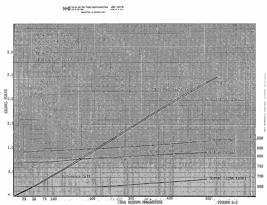
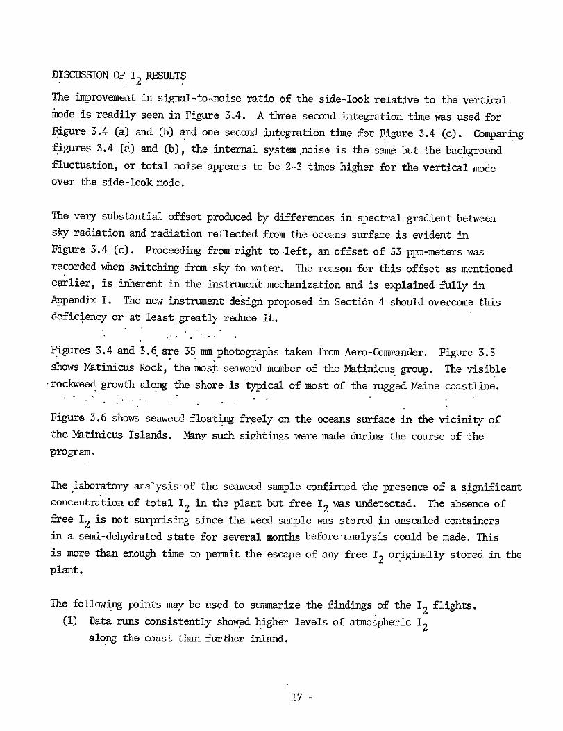
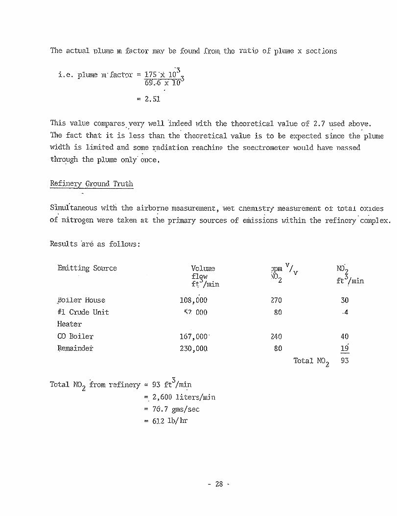
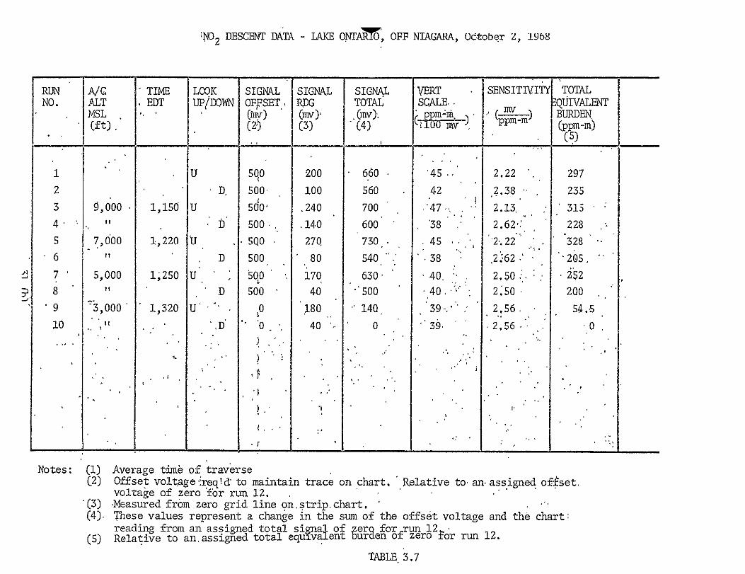
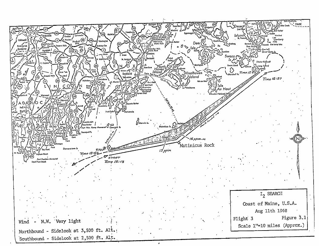
--shy
--
00
15 -1
-
-)C
00
u ~
Cd
100
L
TI
O1
7
C3
-
V~
I -
A
a
V
4
c-
I -
--
toMS
10
__
_
__
_
__
z 4
Hu
cd) 0
A-0-
LHt
H
-
4-44
0
-1
4 d
Zshy
-co rO E
-P
o z rl C14
4shy
-r-= oaf
CD
)
IlD
t-3~N
~~~~j~0 oshyr
t--
4 -S
--shy
rd
I
0 f
Ai-~
-
-O
viO
a 44
C
nn trgt
3F
IGUR
E
3 1 4
FIGU
RE
3-14
)
--------
-
bull lt
-d
-
FICURE 14
I a
C
-
rr-r
-
Y
p bull
Sl
V-rv tAQ
J
-
-
-
-
--
-i--
--
---
-
i-
LUI cO
) 01()
C
JI
LL
I)
oL I=
Ld -gt 2
CJ
oI
OL
L
a
0 b
r
3 0
E- L
(I
o o
u
-) C
7a --shy
0 0
C
af C
t
0 1)
r C
4 E
c iJ
-c
4ZI
-
0I 0)
0
C)o
-4
-r ~
4
X O ~
D
x
IOTO
THE
CE
NTI
ME
FTE
R
25C
m
KE
uF
r9a
amp
fl
CO
46
15
1(
MA
DrIN
l U 6
A
R
FRO
M
ifx 1
L
ts
-
IS I
(D4
ar
a T
Nli
TIt
wlf
N
MI
r
1i
~ i
17_
j~
1I$[
T
4~t
In
Th6
-4
l
r
ffii
irit
__
__
_
-
__
_
6 ~-
4
4 -444 4
I 4 --(4 4 44
4 -
A S-Sn
jv ~ 7
4--
7 A31) 4
I
7-shy
4 --vttArWvi7gt A M0sJ1 lyYiwc u
4 -4 )t~4I 4plusmn ~ ~Vk)~ -~
44 ~
4 4 4--4 4
4 4~ 4
(tQ IT -m DId
44 ---V
~1 A
I r 4 tA-amp)
4 4 4
-C
I
5
4 4
(72) TT~ EIUflDIA t
5
1-~ N
0 ~ lt-gshy
4 -~ 4- 4 (3 -4-- -C U
01
ONTARIO IYDRO
LAKEVIEW GENERATING STATION FROM ABOUT 5000 FT
FIGURE 310
b -
Z
-
-KO
+
y
rr
3
--
-3
v~
-
i-
~~
~ ~~
D CDi
-
-
-
~
~ CD--i
Ao
C
-z2
1
CI
)7
z C) _
l
-
~~ ~
~(
(D
-
--
-
bull
E
shy
~~
~~u -
- 4
--
-
--
0 shy
(D
-
0
i
o
+) --
--- 0
--
-cs -
C
shy
lt
-
--
---
-
----
- --- -
------
degdeg
i- -
i
~~~t
-
C)
-
o
--
o
-
-
lt
M
deg
-~
~~~~ ~
~ 1A
h
-lt
--
~~
~
I
o
s
00
-ww2
2-0
W
0 0
w
Ck)
CL
gt9
FIGU
RE 12
250 - 012SULFUR DIOXIDE r HALF OR LESS 01
200 fl OF DATA VALIDshy150 III 1008
00641
100 p 0 4
50 U 002
F MAMJ J A S ON D J FM AM J J AS fl)
200 1962 1963
006150 NITRIC OXIDE
002
0 S 0AN D J F M J J N D 000 N10ITROGEN DIOXID
150 t004
I Io-- 1 0002 510 0
DO 000 [ JFM AMJJ A S ONG l F MAIJ J A S ON D
300 _0025-Z TOTAL OXIDANT 0 - (not correcled for 0
S150 SO2 inteFerence I 005
plusmn100 0010 0005z 50
u 0 0000 J FMAMj J A SOND J FMAMJ A SND
200- TOTAL HYDROCARBOII
150 3
100 12
00o - CABOAMON AOXDE FAM ASAS NMOI U ri 41JooCF 04 I A S D 0
A M J I A S 0 U D J F MA M J J A S 0 U D 1962 1V63
Seasonal variation of gaseous
pollutant levels for Washington
FIGURE 5-3
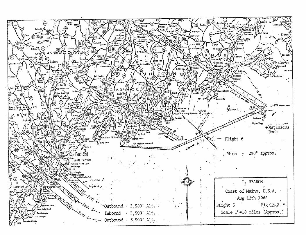
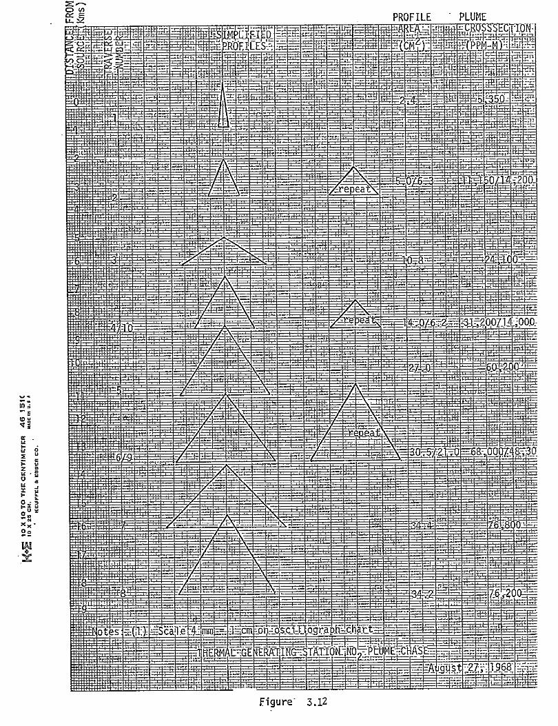