banks’ buffer capital: how important is risk? kjersti-gro ... · pdf filebanks’...
TRANSCRIPT

ANO 2003/11OsloDecember 15, 2003
Working PaperResearch Department
Banks’ buffer capital: How important is risk?
by
Kjersti-Gro Lindquist

ISSN 0801-2504ISBN 82-7553-220-5
Working papers from Norges Bank can be ordered by e-mail:[email protected] from Norges Bank, Subscription service,P.O.Box. 1179 Sentrum N-0107Oslo, Norway.Tel. +47 22 31 63 83, Fax. +47 22 41 31 05
Working papers from 1999 onwards are available as pdf-files on the bank’sweb site: www.norges-bank.no, under “Publications”.
Norges Bank’s working papers presentresearch projects and reports(not usually in their final form)and are intended inter alia to enablethe author to benefit from the commentsof colleagues and other interested parties.
Views and conclusions expressed in working papers are the responsibility of the authors alone.
Working papers fra Norges Bank kan bestilles over e-post:[email protected] ved henvendelse til:Norges Bank, AbonnementsservicePostboks 1179 Sentrum0107 OsloTelefon 22 31 63 83, Telefaks 22 41 31 05
Fra 1999 og senere er publikasjonene tilgjengelige som pdf-filer på www.norges-bank.no, under “Publikasjoner”.
Working papers inneholder forskningsarbeider og utredninger som vanligvisikke har fått sin endelige form. Hensikten er blant annet at forfatteren kan motta kommentarer fra kolleger og andre interesserte.
Synspunkter og konklusjoner i arbeidene står for forfatternes regning.

1
Banks’ buffer capital: How important is risk Kjersti-Gro Lindquist
Norges Bank (Central Bank of Norway), P.O.Box 1179 Sentrum, N-0107 Oslo, Norway.
Tel: +47-22 31 68 73. Fax: +47-22 42 60 62. E-mail: [email protected]
Abstract
Most banks hold a capital to asset ratio well above the required minimum defined by the
present capital adequacy regulation (Basel I). Using bank-level panel data from Norway,
important hypotheses concerning the determination of the buffer capital are analysed. Focus is
on the importance of: (i) risk, particularly credit risk, (ii) the buffer as an insurance, (iii) the
competition effect, (iv) supervisory discipline, and (v) economic growth. A negative or non-
significant risk effect is found, which suggests that introducing a more risk-sensitive capital
regulation (Basel II) is likely to affect Norwegian banks. Support is found for the hypothesis
that buffer capital serves as an insurance against failure to meet the capital requirements.
Keywords: Banking; Excess capital; Risk; Panel data
JEL classification: C33, G21, G32
Acknowledgement: I would like to thank Glenn Hoggarth, Øyvind A. Nilsen, Knut Sandal,
Roger Stover, Martin Summer, Bent Vale, Larry Wall and participants at the Basel
Committee on Banking Supervision’s Workshop in Rome March 2003, the Nordic
Econometric Meeting in Bergen May 2003 and at the Workshop on Bank Competition, Risk,
Regulation and Markets in Helsinki May 2003 for valuable comments and discussions.

2
1. Introduction and motivation
Despite the last decades of market deregulation of the banking industry in many countries,
banking is still one of the most regulated industries in the world. Regulation is in general
justified on the basis of market failures and the importance of preserving financial stability,
although there is still no consensus on how banks should be regulated (Santos (2000)).
As other forms of regulation disappear, capital adequacy regulation becomes relatively more
important, and the result is an increased focus on banks’ capital to asset ratio. In addition, the
experience from banking crises in several countries during the last decades have made both
regulators, supervisory authorities, the banks themselves and probably also their shareholders
more aware of the importance of a sufficient capital to assets ratio. (See Reidhill (2003), for
Norway see Stortinget (1998) and Steigum (2003).) Both the 1988 Basel Capital Accord
(Basel I) and the proposals from the Basel Committee on Banking Supervision to update and
revise this legislation (the forthcoming Basel II) include minimum capital requirements,
although Basel II implies a more risk-sensitive regulation. However, banks’ balance sheets
show that most banks hold a capital ratio well above the required minimum1, and a better
understanding of how these capital buffers are determined and how they vary with risk, across
banks and over time may help us to understand the need for and effect of a new capital
adequacy regulation.
From a regulator’s perspective, one would prefer that banks with a relatively risky portfolio,
i.e. with a high credit risk, hold a relatively high level of buffer capital. Otherwise, these
banks are more likely to fall below the minimum capital ratio, which could give rise to a
credit crunch. Poorly capitalised banks may even spur systemic risk and hence threaten
financial stability. It has been argued that a more risk sensitive capital adequacy regulation
may reduce banks’ willingness to take risk. If banks already risk-adjust their total capital, i.e.
minimum capital plus buffer capital, more than implied by Basel I, replacing Basel I with
Basel II may not affect the capital to asset ratio or risk profile of banks’ portfolio as much as
feared. Therefore, it is clearly of interest to understand how banks’ buffer capital varies with
credit risk under the present regulation.2 1 According to Basel I, banks must hold a “capital to risk adjusted asset” ratio of minimum 8 per cent. In Norway, Basel I was fully implemented in December 1992. 2 The theoretical literature has shown that although capital adequacy regulation may reduce the total volume of risky assets, the composition may be distorted in the direction of more risky assets, and

3
In the literature, it is argued that banks hold excess capital to avoid costs related to market
discipline and supervisory intervention if they approach or fall below the regulatory minimum
capital ratio, see e.g. Furfine (2001). A poorly capitalised bank runs the risk of loosing market
confidence and reputation. Thus, excess capital acts as an insurance against costs that may
occur due to unexpected loan losses and difficulties in raising new capital. The price of
raising new capital, i.e. the required return on equity or interest rate on subordinated debt, is
interpreted as the price of this insurance.3 We expect an increase in price to affect excess
capital negatively. Furthermore, one may argue that the value of this insurance depends on the
uncertainty the bank is facing, i.e. on the probability of experiencing an unexpectedly large
fall in the capital ratio without being able to rebuild this ratio relatively frictionless. If this
“value-argument” is important, the buffer capital should vary positively with the uncertainty
that the bank is facing. However, banks may well behave in accordance with less
sophisticated rules, by for example aiming at a relatively constant buffer.
Unexpected loan losses may be due to purely random shocks or asymmetric information in
the lender-borrower relationship. In the latter case, more extensive screening and monitoring
of borrowers could increase the banks’ understanding of the risk involved in each project (see
Hellwig (1991) for a discussion and references therein). Screening and monitoring are costly,
however, and banks probably balance the cost of and gain from these activities against the
cost of excess capital. In the presence of scale economies in screening and monitoring, one
would expect large banks to substitute relatively less of these activities with excess capital.
Hence, one may find a negative size effect on excess capital. A negative size effect may also
be due to a diversification effect. The argument is that portfolio diversification reduces the
probability of experiencing a large drop in the capital ratio, and that diversification increases
with bank size. A third argument for a negative size effect comes from the “too-big-to-fail”
hypothesis. If large banks expect support from the government in the event of difficulties,
while this is not, to the same degree, expected by small banks, we should expect large banks
to hold lower capital buffers.
average risk may increase. Risk consistent weights are not sufficient to correct for this moral hazard effect in limited liability banks. See Koehn and Santomero (1980), Kim and Santomero (1988), Rochet (1992a,b) and Freixas and Rochet (1997), section 8.3.3). We do not address these issues in this analysis, since we do not include the introduction of capital adequacy regulation or a more risk-sensitive regulation. 3 Norwegian banks face restrictions on the ratio of subordinated debt to equity capital in addition to the minimum capital-ratio requirement.
4
According to Furfine (2001), changes in supervisory monitoring of banks affect their capital
ratios. In the presence of a supervisory discipline effect, we would expect a positive
relationship between supervisory scrutiny and banks’ capital buffer. Furthermore, a bank may
use excess capital as a signal of its solvency or probability of non-failure. Hence, excess
capital may serve as an instrument, which the bank is willing to pay for, in the competition for
unsecured deposits and money market funding. We, therefore, expect banks to care about
their relative buffer, i.e. the size of their own capital buffer relative to those of their
competitors.
Berger, Herring and Szegö (1995) argue that banks may hold excess capital to be able to
exploit unexpected investment opportunities. Although the relevance of this argument is
likely to depend on how difficult it is for the bank - on very short notice – to increase its
capital, one may expect banks’ buffer capital to decline in periods with high economic
growth, since more interesting investment projects are likely to exist. The variation in the
buffer capital over the business cycle may be of interest also from the perspective of the pro-
cyclicality of both the present and the forthcoming capital legislation.4 As a result of their
evaluation of future risk and investment opportunities today contra tomorrow, banks may use
their buffer capital to either dampen or increase the pro-cyclical effects embedded in the
legislation. However, a systematic relationship between economic growth and buffer capital
must be interpreted with care, since the change in buffer capital may reflect changes in the
volume of capital as well as in the volume of loans.
In this paper, we analyse empirically the relationship between banks’ credit risk and buffer
capital. A reduced form framework is applied, hence controlling for other variables of
importance for the determination of the buffer capital.5 We focus on the issues discussed
above: i) Whether excess capital depends on the risk profile of the banks’ portfolios,
particularly the credit risk involved, ii) Whether excess capital acts as an insurance against
falling below the required minimum capital to asset ratio, iii) Whether banks use excess
4 See, among others, Basel Committee on Banking Supervision (2001), Borio et al. (2001), Danielsson, Embrechts, Goodhart, Keating, Muennich, Renault and Shin (2001) and European Central Bank (2001) for a discussion of the pro-cyclicality issue. 5 An alternative approach is to model banks’ total capital ratio as in Barrios and Blanco (2003). They argue that some banks are affected while others are not affected by the capital adequacy regulation. To describe the behaviour of these two types of banks they develop a regulatory model and a market model. In this paper, we assume that the behaviour of all banks is affected by the current regulation and test for market effects and in addition a supervisory discipline effect.
5
capital as a signal, i.e. a competition parameter, and relative capital buffers matter, iv)
Whether the level of supervisory monitoring matters, and v) Whether the buffer capital
depends on economic growth.
We also emphasise bank heterogeneity, which, within a financial stability framework, is
clearly important. Although the (arithmetic) average buffer capital of Norwegian banks has
varied around 8-12 per cent since the early 1990s, i.e. the average capital ratio of Norwegian
banks’ is around twice the required minimum level, the data show important variation across
banks. It is clearly of interest to understand how the buffer capital of different banks or groups
of banks is connected to the different factors discussed above. In the empirical part, we split
the banks in two sub-groups, i.e. savings banks and commercial banks. Their behaviour is
likely to vary systematically, and the average buffer capital of savings banks is in general well
above that of commercial banks. In Norway, there is a relatively large number of small and, in
general, locally-based savings banks and a small number of larger commercial banks, of
which some have branches across the country. While the capital of commercial banks
basically consists of equity capital, accumulated retained profits and subordinated debt, the
capital of savings banks is very much based on accumulated retained profits and a hybrid
capital instrument intended to mimic equity capital. This hybrid capital instrument does not
give the holder the same right as share holders in commercial banks to vote at a general
meeting, however. Traditionally, these two groups of banks have served different purposes.
While savings banks have served as intermediaries for a local population, granting mortgage
loans and loans to small businesses, commercial banks have also served large commercial
customers. In addition, commercial banks have been profit-making businesses with pressure
to maximise shareholders’ returns. The philosophy of savings banks has been to offer loans
and deposit accounts with favourable interest rates.
Section 2 presents the model to be estimated. The data and empirical results are discussed in
Section 3. Section 4 concludes, and the Appendix presents the empirical variables in more
detail.
2. The model
In the empirical analysis of banks’ buffer capital, our starting point is Ayuso, Pérez and
Saurina (2002), who analyse the behaviour of the buffer capital of Spanish banks using annual

6
data for 1986-2000. We add to the literature in several ways. First, we take explicitly into
account the “insurance against falling below the required minimum capital ratio” argument.
Second, we take into account that relative capital buffers may matter due to competition.
Third, to test the conclusion in Furfine (2001) that a supervisory discipline effect is present,
we include a variable that represents the supervisory authorities’ monitoring of banks. Fourth,
we analyse the importance of banks’ risk for the buffer capital. We apply a more sophisticated
credit-risk measure than Ayuso et al. Fifth, while Ayuso et al. include fixed effects in their
model and a shift parameter for small and large banks, we apply a random effect approach and
estimate the model on two sub-groups of banks, i.e. savings banks and commercial banks.
This allows all slope coefficients to vary across the two sub-groups.
Our most general model is defined in Eq. (1). Subscripts i and t denote bank and period
respectively. Small letters indicate data on logarithmic form, i.e. buf=ln(BUF), pec=ln(PEC),
etc. Lags in explanatory variables are introduced to avoid simultaneity problems.
bufit = α0i + α1 riskit + α2 peci,t-1 + α3 vprofi,t-1 + α4 cbuft-1 + α5 supt + α6 gdpgt (1)
+ α7 sizeit + α8 uslpi,t-1 + α9 trendt + α10 Q2 + α11 Q3 + α12 Q4 + uit
where BUF is the capital buffer measured as the “excess-capital to risk-weighted asset” ratio;
RISK represents the bank’s credit risk. A measure based on predicted bankruptcy
probabilities of limited liability firms and loss given default is applied; PEC is the price of
excess capital. Two alternative empirical proxies are applied. (i) The lagged predicted interest
rate on subordinated debt (PEC1i,t-1), which varies both over time and across banks, and (ii)
the β-coefficient (PEC2t) of the banking industry6, which varies over time but not across
banks; VPROF is the variance of each bank’s quarterly profits calculated over past
observations; CBUF is the competitors’ average capital buffer calculated separately for the
two groups, i.e. for savings banks and commercial bank. Banks are expected to compete most
heavily with banks of the same category; SUP represents supervisory scrutiny and is
measured by the number of on-site inspections by the supervisory authority in Norway, i.e.
the Banking, Insurance and Securities Commission; GDPG denotes the four-quarter growth
rate of gross domestic product; SIZE is total financial assets incl. guarantees and represents
bank size; USLP is the stock of unspecified loan loss provisions relative to risk-weighted
6 The β-coefficient is calculated in accordance with the Sharpe-Lintner capital asset pricing model (CAPM), and reflects, in our setting, the risk premium of investing in the Norwegian banking industry as compared to the Oslo Stock Exchange All Share Index. More details are given in the Appendix.
7
assets; TREND is a simple deterministic trend variable; Q2, Q3, Q4 are quarterly dummy
variables included to capture seasonal effects; u is an added disturbance. A more detailed
presentation of the empirical variables is given in the Appendix.
We have calculated and applied alternative empirical proxies for the risk profile of banks,
RISK, but the empirical results are qualitatively independent of the choice of empirical
variable.7 Banks may vary significantly in their willingness to take risk, and the measures of
risk-profile are assumed to contain information on bank type with respect to this. Although
Basel I includes some risk sensitivity in the calculation of the capital requirement, it is in
general assumed to be too rude, with the consequence that risk is not properly taken into
account. Therefore, if banks consider the true credit risk of their portfolios when deciding on
the total amount of capital, one would expect the buffer capital to vary positively with any
risk measure that is closer to replicate the true risk profile of banks’ portfolios than the risk
weights in Basel I.
The motivation for including the price of excess capital, PEC, and the variance of each bank’s
past profits, VPROF, is to analyse how sophisticated insurance rules banks are following.
While the price is assumed to reflect the development in the insurance premium, and hence
represents a price effect, the variance of profits is assumed to reflect how valuable this
insurance is for the bank. The banks can increase their buffer capital through retained profits,
but this is an uncertain option if profits are highly variable. The probability of falling below
the required minimum level of the capital ratio is therefore assumed to increase with VPROF.
The value of the buffer capital, and hence also the buffer capital, are expected to vary
positively with VPROF.
VPROF and RISK are related, since both capture information about risk. Both measures
should therefore be taken into account when interpreting the importance of risk for banks’
buffer capital.
7 Other measures for RISK applied in the analysis are: (i) The risk-weighted to unweighted assets ratio. The risk-weighted assets are calculated in accordance with the Basel I rules. This measure takes values between zero and one, and increasing value implies increasing risk. (ii) Twelve quarters moving average of the flow variable loan loss provisions relative to total assets. Ayoso et al. (2002) use the ratio of non-performing loans to total loans and credits as a risk measure. This is comparable with our measure (ii), since banks with non-performing loans are obliged to make provisions for loan losses.
8
The GDPG variable is included to capture economic growth effects. Our observation period
does not include a whole business cycle, and the effect of this variable should therefore be
interpreted with care and not used to draw conclusions about business cycle effects.
To some degree, banks have the option of making unspecified loan loss provisions. From the
insurance against “falling below the minimum capital requirement” perspective, this
represents an alternative to increasing the capital buffer. Therefore, we expect USLP to have a
negative effect on the buffer.
The trend variable, TREND, is included to capture secular changes in the capital buffer not
captured by the other variables, see Furfine (2001) and Boyd and Gertler (1994). However,
the increased importance of off-balance-sheet items, such as letters of credit and loan
commitments, is taken into account in the calculation of the capital buffer, and hence this
should not give rise to trend effects in the capital buffer. In principle, the trend effect
represents the net trend effect of all excluded variables.
We expect α2 < 0, α3 > 0, α4 > 0, α5 > 0, α7 < 0 and α8 < 0. If α1 > 0, then banks with more
risky assets have a higher buffer capital, and if α1 < 0 the opposite is true. The economic
growth and trend effects, represented by α6 and α9 respectively, and the seasonal effects,
represented by α10, α11 and α12, can in principle take any sign.
3. Data and empirical results
The data
To estimate Eq. (1), we use an unbalanced bank-level panel data set for Norwegian banks.
Primarily we use quarterly financial statements that all banks are obliged to report to Norges
Bank, combined with Norwegian national account data and information from the Banking,
Insurance and Securities Commission. The data applied cover the period 1995q4-2001q4, i.e.
25 quarters. The regressions start in 1996q1 due to a lag in explanatory variables, however.
We have access to most of the data back to 1991q4, but we have chosen not to include the
early 1990s in our sample for two reasons. First, in 1991-1992 banks were adjusting their
capital ratios in accordance with the forthcoming Basel I capital adequacy requirements,
which were fully implemented for Norwegian banks by 31 December 1992. Second, during
the 1988-1992 banking crisis in Norway, many banks saw their capital erode. In the following
9
years, banks rebuilt their buffer capital, and we need to exclude these years so that
extraordinary behaviour will not affect the results. Most likely, the rebuilding of capital
buffers was finished before early 1996, but the data needed to calculate the empirical proxies
for the price on excess capital (PEC) are unavailable prior to this year.
The dataset used for estimation includes 3401 observations. None of the banks in our sample
have a capital ratio below the required minimum level. We have excluded only three
observations due to missing observations on explanatory variables. The sub-sample for
savings banks consists of 3101 observations on 131 different banks, of which 127 banks are
observed over the whole estimation period. The sub-sample for commercial banks is much
smaller and consists of 300 observations on 16 different banks, of which 10 are observed over
the whole estimation period. The variables used in the analysis are summarised in Table 1.
Table 1. Main features of the data, 1996q1-2001q4. Bank specific variables are based on 3101 observations on savings banks and 300 observations on commercial banks Variable Mean Std. dev. Minimum Maximum
BUFi 9.379 5.963 0.069 38.333
RISKi 0.016 0.005 0.004 0.043
PEC1ia 2.008 0.181 1.175 2.871
PEC2a 0.750 0.343 0.191 1.512
VPROFi 17776 146248 0.003 2360498
CBUFi 12.120 23.155 3.919 366.383
SUP 11.377 1.027 10.000 12.750
GDPGb 3.012 2.226 -0.372 7.991
SIZEic 497 2861 1 3.2·104
USLPi 0.010 0.006 1.0·10-7 0.040 a PEC1 is the predicted interest rate on subordinated debt. A systematic measurement error affects the level of this interest rate. PEC2 is the β-coefficient of the banking industry. b Mainland-Norway, i.e. excess oil, natural gas and shipping. c NOK mill.
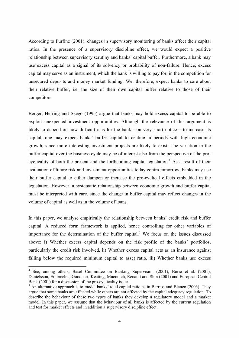
Figure 1-5 show the development over time in some of the variables. We calculate quarterly
arithmetic means and split between savings banks and commercial banks. To better see the
development over time, we include some years prior to our estimation period. Figure 1 shows
that after the banking crisis, both savings banks and commercial banks built up their buffer
capital (BUF). Although the buffer capital of savings banks was as high as 8-9 per cent in

10
1992, banks gradually increased their buffer capital until reaching a top in late 1995. Then the
positive trend was reversed, and the buffer capital of savings banks declined steadily until
reaching 8-9 per cent again in 2000/2001. Commercial banks started out with a buffer capital
of 4 per cent in 1992. The buffer capital was more than doubled through 1993, i.e. in one year
only, but then a long period with declining buffer capital started, which brought it down
below 3 per cent. A reversion with increasing buffer capital started in late 1997. It is
interesting to note that the buffer capital of savings banks in particular seems to follow a
systematic seasonal pattern with a peak in the fourth quarter.
Figure 1. Buffer capital, per cent of risk weighted assets. Quarterly unweighted means
24
68
1012
Buf
fer c
apita
l
1992q3 1995q1 1997q3 2000q1 2002q3Date
Savings banks Commercial banks
Note: Assets are risk-weighted in accordance with Basel I rules.
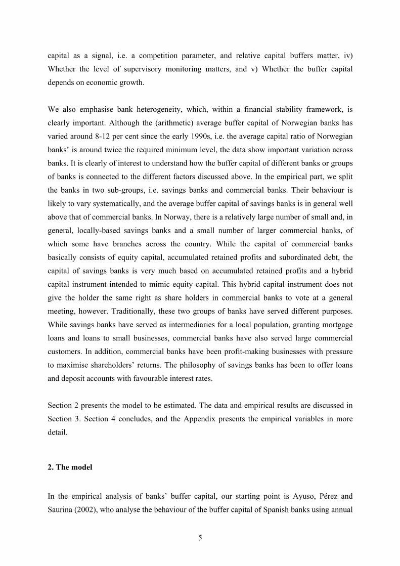
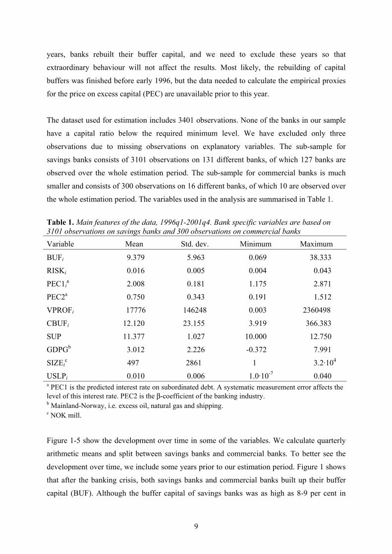
Figure 2 shows the cumulative variance of quarterly profits (VPROF), i.e. the variance of
previous profits. The smooth development in the mean of VPROF conceals a more erratic
picture at the bank level.
11
Figure 2. Cumulative variance of banks’ quarterly profits. Quarterly unweighted means, 1992q3=100
100
200
300
400
Var
ianc
e
1992q3 1995q1 1997q3 2000q1 2002q3Date
Savings banks Commercial banks
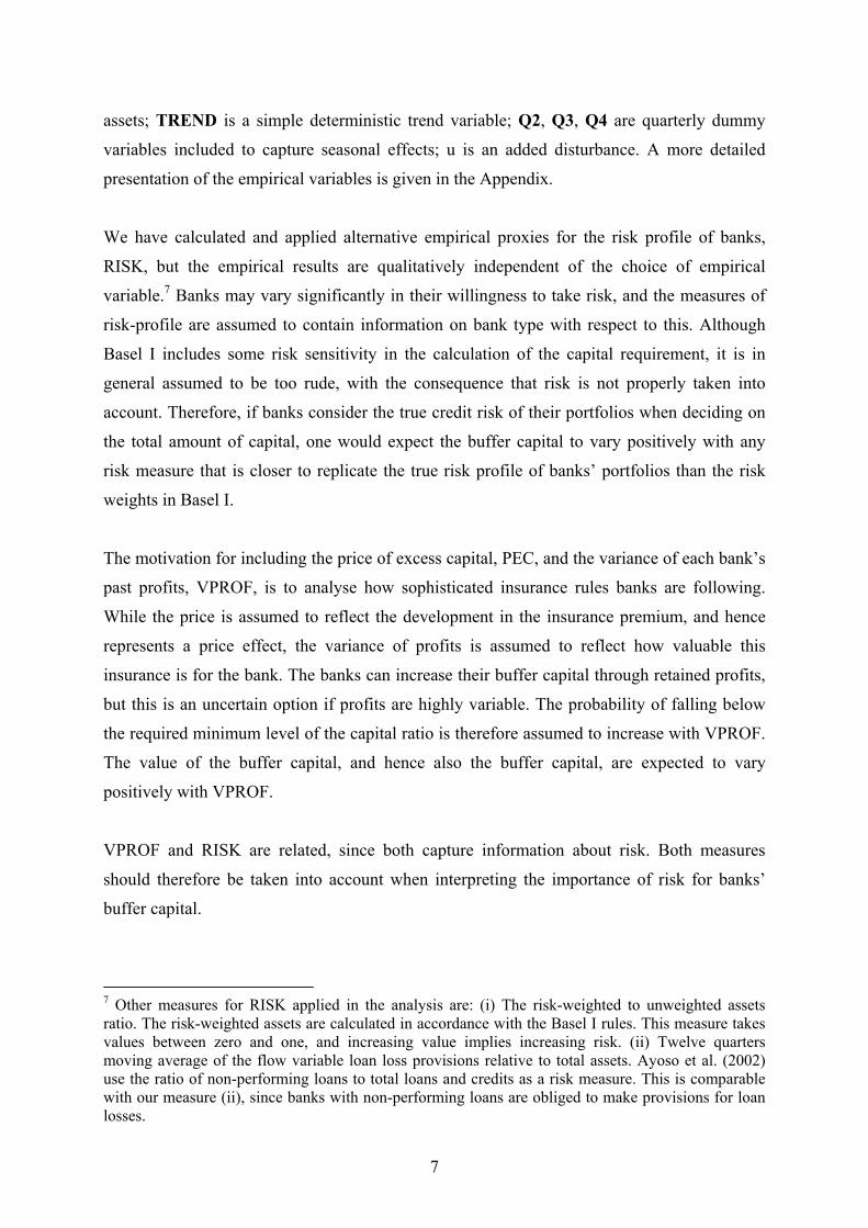
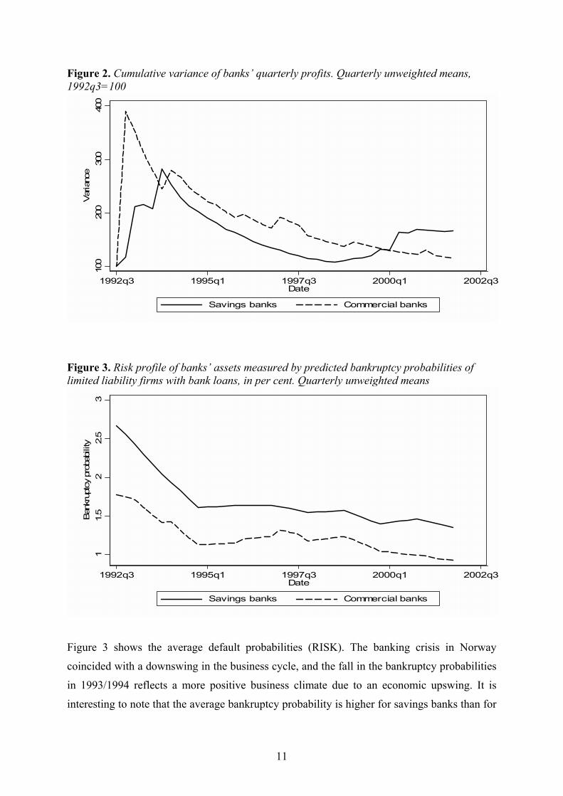
Figure 3. Risk profile of banks’ assets measured by predicted bankruptcy probabilities of limited liability firms with bank loans, in per cent. Quarterly unweighted means
11.
52
2.5
3Ban
krup
tcy
prob
abili
ty
1992q3 1995q1 1997q3 2000q1 2002q3Date
Savings banks Commercial banks
Figure 3 shows the average default probabilities (RISK). The banking crisis in Norway
coincided with a downswing in the business cycle, and the fall in the bankruptcy probabilities
in 1993/1994 reflects a more positive business climate due to an economic upswing. It is
interesting to note that the average bankruptcy probability is higher for savings banks than for
12
commercial banks. This reflects that savings banks in general lend to business sectors and
counties with relatively high bankruptcy probabilities, such as the hotel and restaurant sector.
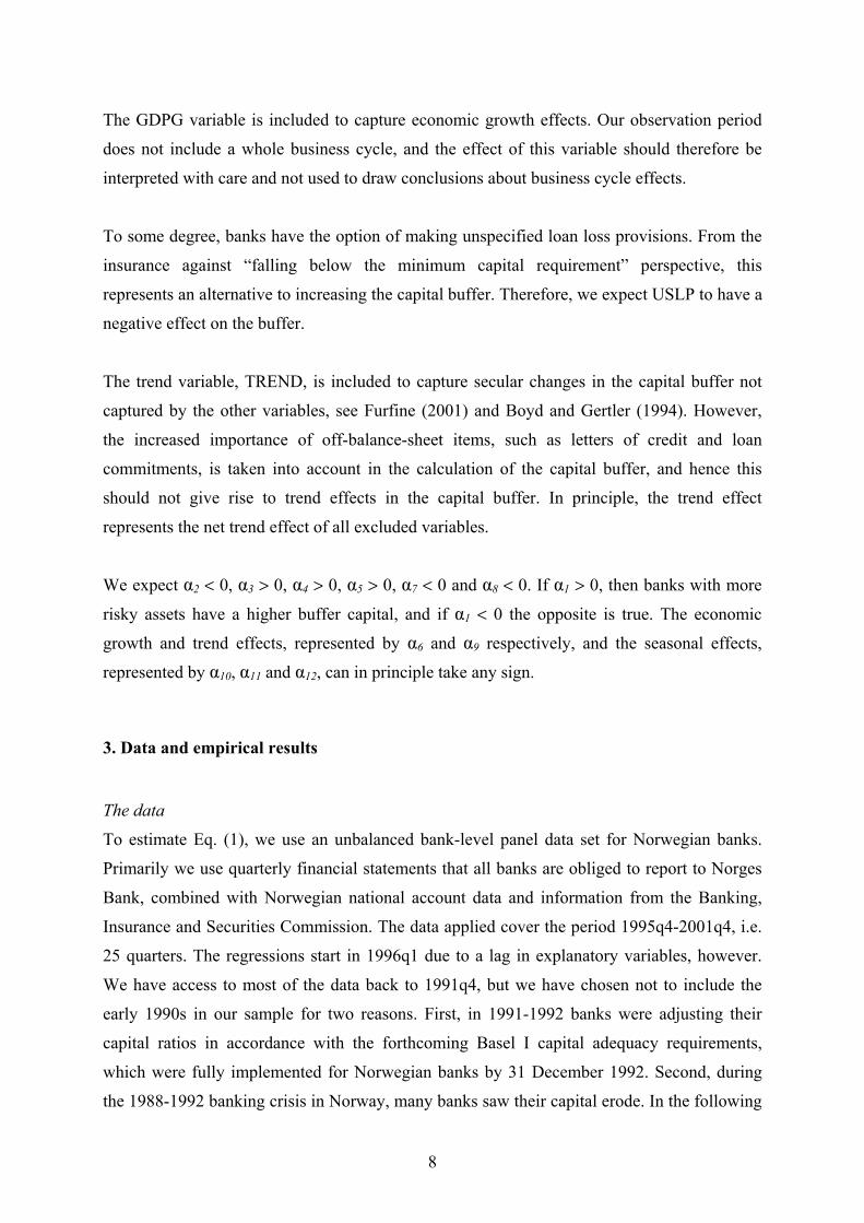
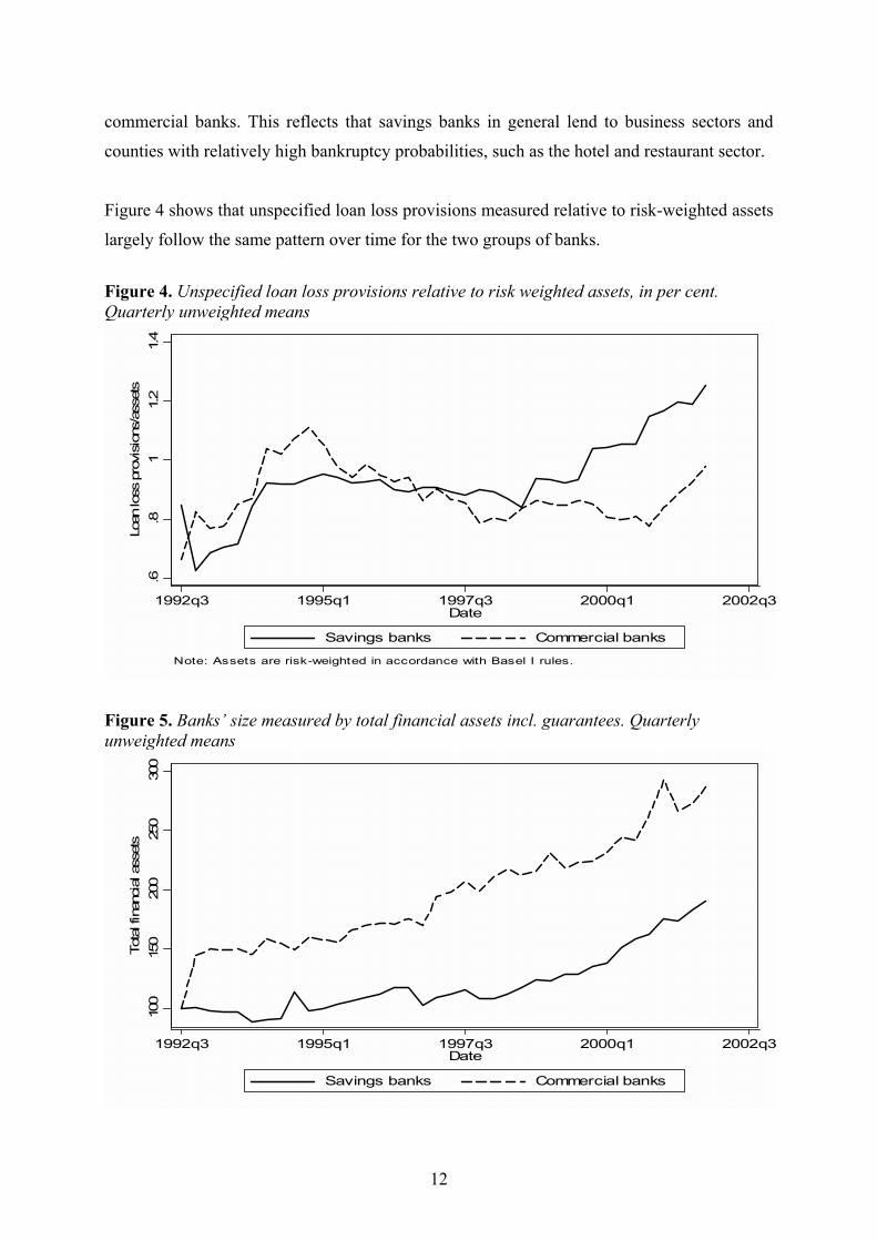
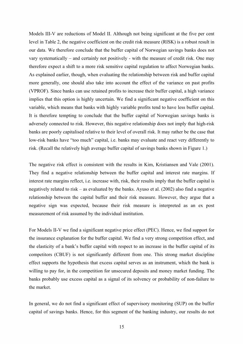
Figure 4 shows that unspecified loan loss provisions measured relative to risk-weighted assets
largely follow the same pattern over time for the two groups of banks.
Figure 4. Unspecified loan loss provisions relative to risk weighted assets, in per cent. Quarterly unweighted means
.6.8
11.
21.
4Lo
an lo
ss p
rovi
sion
s/as
sets
1992q3 1995q1 1997q3 2000q1 2002q3Date
Savings banks Commercial banks
Note: Assets are risk-weighted in accordance with Basel I rules.
Figure 5. Banks’ size measured by total financial assets incl. guarantees. Quarterly unweighted means
100
150
200
250
300
Tota
l fin
anci
al a
sset
s
1992q3 1995q1 1997q3 2000q1 2002q3Date
Savings banks Commercial banks

13
From Figure 5 it is clear that, measured by total financial assets incl. guarantees, the average
size of both bank types has increased over time. The increase is larger for commercial banks
than for savings banks.
Empirical results
We estimate Eq. (1) for savings banks and commercial banks separately assuming random
effects. This implies a time-invariant bank specific effect on the level of the buffer capital,
while the slope coefficients, i.e. the estimated elasticities, are equal across banks within the
two groups but may vary across the two groups. We use the Generalised Least Squares (GLS)
Random-Effects Model procedure in STATA 7.0 (StataCorp (2001)). The Breusch and Pagan
(1980) Lagrange multiplier test, which tests if the variance of the random component is zero,
is applied to test the relevance of the random effects specification. To test the appropriateness
of the random effects estimator applied, which assumes that the random effects and the
regressors are uncorrelated, we apply the Hausman (1978) specification test. The estimation
results for savings and commercial banks are given in Table 2 and Table 3 respectively.
According to the results in Table 2, the hypothesis of “no random effects” is clearly rejected,
while the hypothesis of “no correlation between the random effects” in general is not. Model I
and II, which both represent our most general model, differ with respect to the information set
used, i.e., different empirical proxies for the price variable (PEC) are applied. In Model I, we
use the predicted bank specific interest rate on subordinated debt lagged one period (PEC1),
while in Model II, and in the remaining models, we use the β-coefficient (PEC2). In general,
we do not find significant price effects when applying the first measure, and we therefore
concentrate on the results from using the β-coefficient, i.e. PEC2. The poor results when
using PEC1 may reflect that the generalisation from the relatively small number of savings
banks included in the estimation of the interest rate on subordinated debt is not valid.

14
Table 2. Estimation results for savings banks. Endogenous variable is bufit
a
Variable Model I Model II Model III Model IV Model V const 1.766 -0.679 -0.038 0.169 0.064 (2.62) (-0.88) (-0.20) ( 1.29) ( 0.87) riskit -0.019 -0.037 -0.041 (-0.69) (-1.34) (-1.51) peci,t-1
b -0.053 -0.069 -0.066 -0.066 -0.069 (-0.63) (-6.71) (-7.21) (-7.18) (-8.11) vprofi,t-1 -0.032 -0.064 -0.064 -0.063 -0.064 (-2.51) (-4.99) (-4.96) (-4.89) (-5.02) cbufi,t-1 0.544 1.075 0.978 0.960 1.000c
(3.63) (7.33) (22.81) (23.28) supt 0.105 0.032 (2.06) (0.71) gdpgt 0.002 -0.055 -0.052 -0.049 -0.063 (0.08) (-1.81) (-1.92) (-1.83) (-2.80) uslpi,t-1 0.005 -0.002 (1.77) (-0.60) sizeit -0.052 -0.021 -0.021 -0.020 -0.018 (-5.29) (-3.37) (-3.26) (-3.18) (-3.03) trendt -0.223 0.091 (-1.82) ( 0.78) Q2 -0.029 -0.056 -0.056 -0.056 -0.057 (-2.56) (-4.67) (-4.69) (-4.71) (-4.80) Q3 -0.063 -0.046 -0.050 -0.051 -0.049 (-5.12) (-3.58) (-4.44) (-4.51) (-4.41) Q4 0.108 0.159 0.150 0.149 0.154 (6.53) (8.93) (12.23) (12.15) (14.08) R2 : Within 0.263 0.269 0.268 0.267 0.136 Between 0.168 0.110 0.111 0.115 0.113 Overall 0.191 0.137 0.137 0.140 0.114 REd 0.000 0.000 0.000 0.000 0.000 Hausmane 0.007 0.209 0.393 0.127 0.461 a t-values in parentheses. The number of observations is 3101, and the number of banks is 131. b In Model I, we use the lagged predicted interest rate on subordinated debt which varies both over time and across banks. In Models II-V, we use the β-coefficient which is constant across banks. c Restricted a priori. d Breusch and Pagan (1980) Lagrange multiplier test. H0 is no random effects. Prob>χ2(1) is reported. e Hausman’s (1980) specification test. H0 is zero correlation between the random effects and the explanatory variables. Prob>χ2(5) is reported.
15
Models III-V are reductions of Model II. Although not being significant at the five per cent
level in Table 2, the negative coefficient on the credit risk measure (RISK) is a robust result in
our data. We therefore conclude that the buffer capital of Norwegian savings banks does not
vary systematically – and certainly not positively - with the measure of credit risk. One may
therefore expect a shift to a more risk sensitive capital regulation to affect Norwegian banks.
As explained earlier, though, when evaluating the relationship between risk and buffer capital
more generally, one should also take into account the effect of the variance on past profits
(VPROF). Since banks can use retained profits to increase their buffer capital, a high variance
implies that this option is highly uncertain. We find a significant negative coefficient on this
variable, which means that banks with highly variable profits tend to have less buffer capital.
It is therefore tempting to conclude that the buffer capital of Norwegian savings banks is
adversely connected to risk. However, this negative relationship does not imply that high-risk
banks are poorly capitalised relative to their level of overall risk. It may rather be the case that
low-risk banks have “too much” capital, i.e. banks may evaluate and react very differently to
risk. (Recall the relatively high average buffer capital of savings banks shown in Figure 1.)
The negative risk effect is consistent with the results in Kim, Kristiansen and Vale (2001).
They find a negative relationship between the buffer capital and interest rate margins. If
interest rate margins reflect, i.e. increase with, risk, their results imply that the buffer capital is
negatively related to risk – as evaluated by the banks. Ayuso et al. (2002) also find a negative
relationship between the capital buffer and their risk measure. However, they argue that a
negative sign was expected, because their risk measure is interpreted as an ex post
measurement of risk assumed by the individual institution.
For Models II-V we find a significant negative price effect (PEC). Hence, we find support for
the insurance explanation for the buffer capital. We find a very strong competition effect, and
the elasticity of a bank’s buffer capital with respect to an increase in the buffer capital of its
competitors (CBUF) is not significantly different from one. This strong market discipline
effect supports the hypothesis that excess capital serves as an instrument, which the bank is
willing to pay for, in the competition for unsecured deposits and money market funding. The
banks probably use excess capital as a signal of its solvency or probability of non-failure to
the market.
In general, we do not find a significant effect of supervisory monitoring (SUP) on the buffer
capital of savings banks. Hence, for this segment of the banking industry, our results do not

16
support the conclusion in Furfine (2001). The negative relationship between economic growth
(DGDP) and buffer capital is consistent with the argument in Berger et al. (1995) that banks
hold excess capital to be able to exploit unexpected investment opportunities. However, this is
not a very strong conclusion, since the buffer capital may vary systematically with growth due
to changes in banks’ capital rather than assets. We do not find a significant effect of
unspecified loan-losses provisions (USLP) on the buffer capital of savings banks.
We find, however, a clear negative size (SIZE) effect, which, as explained earlier, may be due
to several factors. A higher level of monitoring and screening in large banks due to scale
economies in these activities may reduce the need for buffer capital as an insurance. The
negative size effect may also come from a diversification effect not captured by the measure
of credit risk (RISK). A third explanation is related to the too-big-to-fail hypothesis. The
estimated Models II-V do not include a significant trend effect. We find, however, systematic
seasonal variation in the buffer capital, as suggested by the significant coefficients of the
quarterly dummy-variables (Q2-Q4). The estimated quarterly effects imply that banks scale
down their buffer capital over the three first quarters of the year. The explanation to this
pattern is that savings banks use retained profits to adjust their capital, and this is basically
done in the fourth quarter when the financial statement is revised. According to the estimated
model, the buffer capital increases by more than 1½ percentage point from the third to the
fourth quarter.
The results for commercial banks are less clear cut. We use a general to specific modelling
strategy, and, to some degree, the reduced model depends on the route taken in the reduction
process. Less robust conclusions for the commercial banks than for the savings banks are
probably due to the much smaller cross-sectional dimension of the sub-sample with
commercial banks. One may therefore argue in favour of a combined regression, i.e. a
regression based on all data for both groups of banks. However, because savings banks
dominate in the combined regression, these results are very close to those given in Table 2.
In Table 3, we summarize the main differences across competing models for commercial
banks. Again, we find that the hypothesis of “no random effects” is clearly rejected, while the
hypothesis of “no correlation between the random effects” in general is not. As in Table 2,
Model I and Model II correspond to our most general model, but they differ with respect to
the price variable applied. In contrast to savings banks, we generally find a positive price
effect for commercial banks. This probably reflects some incidental co-movement of the data.
17
According to the estimated interest rate equations (see the Appendix), the interest rate on
subordinated debt largely follows the risk-free interest rate, i.e. the interest rate on 10-year
government bonds. The buffer capital of commercial banks and this risk-free interest rate
happens to follow a very similar pattern over our estimation period, and this explains the
positive price elasticity.
To avoid the problem described above, we exclude the price variables from our model. The
results from this strategy are given in Models III-V. In Model III, an attempt is made to
include price effects without including a price variable that largely follows the same trend as
the risk-free interest rate. We estimate the model for the buffer capital including the bank
specific explanatory variables of the interest rate equation, i.e. we include a variable that
measures the four-quarter average of losses relative to assets (LOSSASS). The second bank
specific variable, i.e. size, is already included in the model. Again, we find a positive
relationship between the buffer capital and the variable intended to represent the price. This
result may help us understand the mechanisms driving the buffer capital of commercial banks,
however. The positive relationship between previous losses to assets and the buffer capital
suggests that commercial banks put much effort into rebuilding the buffer capital after a
period of losses independent of price. Remember that commercial banks in general have a
much smaller buffer capital than savings banks. Although we do not find a negative price
effect or a positive effect of the variability in profits, the positive losses-to-assets effect may
represent both an insurance effect and a market discipline effect. We conclude that
commercial banks seem to follow a very simple insurance rule, i.e., conditional on variables
in the model which represent other explanations and motivations for why banks hold capital
buffers, banks tend to keep a relatively stable capital buffer and rebuild this buffer when
experiencing losses.
In contrast to the results for the savings banks, Table 3 shows that for commercial banks we
have a robust positive effect of supervisory scrutiny (SUP) on the buffer capital. Hence, an
increase in the activity by the supervisory authorities, i.e. an increase in the number of on-site
inspections, increases the buffer capital of commercial banks. Although not always
significant, we generally find a negative GDP-growth effect. With the same reservation as for
the savings banks, one may argue that this supports the hypothesis that banks hold excess
capital to exploit unexpected investment opportunities. The negative third quarter (Q3)
seasonal effect is very robust.
18
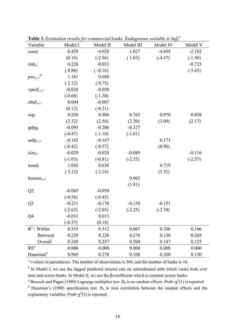
Table 3. Estimation results for commercial banks. Endogenous variable is bufit
a
Variable Model I Model II Model III Model IV Model V const 0.429 -4.028 1.027 -4.895 -2.182 (0.16) (-2.96) ( 1.03) (-4.47) (-1.56) riskit 0.228 -0.033 -0.723 ( 0.80) ( -0.16) (-3.65) peci,t-1
b 1.181 0.048 ( 2.12) ( 0.75) vprofi,t-1 -0.026 -0.050 (-0.68) (-1.30) cbufi,t-1 0.004 -0.007 (0.12) (-0.21) supt 0.926 0.966 0.765 0.970 0.858 (2.32) (2.56) (2.20) (3.09) (2.17) gdpgt -0.095 -0.206 -0.327 (-0.47) (-1.10) (-1.81) uslpi,t-1 -0.162 -0.167 0.171 (-8.42) (-8.57) (8.90) sizeit -0.029 -0.020 -0.089 -0.116 (-1.03) (-0.81) (-2.55) (-2.57) trendt 1.042 0.638 0.719 ( 3.12) ( 2.18) (3.51) lossassi,t-1 0.065 (1.81) Q2 -0.045 -0.039 (-0.56) (-0.45) Q3 -0.231 -0.170 -0.158 -0.151 (-2.62) (-2.05) (-2.25) (-2.38) Q4 -0.031 0.013 (-0.37) (0.16) R2 : Within 0.355 0.312 0.067 0.306 0.106 Between 0.229 0.226 0.276 0.130 0.268 Overall 0.249 0.257 0.204 0.147 0.125 REc 0.000 0.000 0.000 0.000 0.000 Hausmand 0.969 0.278 0.108 0.300 0.130 a t-values in parentheses. The number of observations is 300, and the number of banks is 16. b In Model I, we use the lagged predicted interest rate on subordinated debt which varies both over time and across banks. In Model II, we use the β-coefficient which is constant across banks. c Breusch and Pagan (1980) Lagrange multiplier test. H0 is no random effects. Prob>χ2(1) is reported. d Hausman’s (1980) specification test. H0 is zero correlation between the random effects and the explanatory variables. Prob>χ2(5) is reported.

19
For the other explanatory variables in Model III-V the sign is generally robust across different
specifications, but the significance of each variable depends on the vector of explanatory
variables included. We generally find a negative credit risk (RISK) effect, and although not
significant in all alternative specifications, we conclude that the buffer capital of commercial
banks does not increase with credit risk. Hence, banks with a higher credit risk probably run a
higher risk of approaching or falling bellow the minimum capital requirement than banks with
a low credit risk. We generally find a negative relationship between buffer capital and
unspecified loan loss provisions (USLP), which suggests that commercial banks may use
unspecified loan loss provisioning as an alternative to building up buffer capital. If a bank
sees problems ahead, by increasing unspecified loan loss provisions rather than the buffer
capital, it is less likely to be criticised by the shareholders for not increasing its lending. As
for savings banks, we find a negative size (SIZE) effect for commercial banks. The trend
(TREND) effect is generally positive, i.e., there is a positive trend in the buffer capital of
commercial banks that cannot be explained by the other variables included in the model.
4. Conclusions
Using unbalanced bank-level panel data for Norway, we estimate a model for banks’ buffer
capital. Buffer capital is defined as the ratio of excess capital to risk-weighted assets. We
focus on the following issues: i) Whether excess capital depends on the risk profile of the
banks’ portfolios with focus on credit risk, ii) Whether excess capital acts as an insurance
against falling below the regulatory minimum capital-ratio, iii) Whether banks use excess
capital as a signal, i.e. a competition parameter, and relative capital buffers matter, iv)
Whether a supervisory discipline effect is present, and v) Whether the buffer capital depends
on economic growth.
We estimate the model separately on two sub-groups of the banks, i.e. on savings banks and
commercial banks. The motivation for this split is that they probably behave differently, and
the level of the buffer capital is in general much higher for savings banks than for commercial
banks.
The results for savings banks suggest that there is a negative relationship between their buffer
capital and risk. The effect of credit risk is not significant, but we find a significant negative
effect of the variance of previous profits, which is interpreted as a broad risk measure. This is

20
a rather thought-provoking result. However, it does not necessarily imply that high-risk banks
are poorly capitalised, and may rather reflect that low-risk banks have “too much” capital. It is
interesting that banks seem to evaluate and react differently to risk. We find a negative price
effect on the buffer capital for savings banks, which supports the hypothesis that banks use
buffer capital as an insurance against costs related to market discipline and supervisory
intervention if they approach or fall below the regulatory minimum capital-ratio. Furthermore,
an elasticity of approximately one on the buffer capital of competitors supports the
assumption that banks use the buffer capital as a signal to the market of solvency and
probability of non-failure. With the reservation that banks may adjust their capital rather than
their assets, a negative relationship between the buffer capital and growth is consistent with
the assumption that banks hold excess capital to exploit unexpected investment opportunities.
There is a systematic variation in the buffer capital with bank size, and large banks tend to
hold a smaller buffer than small banks.
For commercial banks, the results are less clear-cut and robust, which is probably due to the
much smaller cross-sectional dimension of this sub-sample. Irrespective of the choice of
empirical proxy, we generally find a positive price elasticity for commercial banks. This is
probably due to incidental co-movement of the data along the time dimension, and we
therefore exclude the price variables from the model, implicitly assuming no price effects on
the buffer capital of commercial banks. Although not always significant, we generally find a
negative credit-risk effect. As for savings banks, we therefore conclude that the buffer capital
of commercial banks does not increase with credit risk. Hence, the introduction of Basel II is
likely to affect both savings and commercial banks. We find evidence of a supervisory
discipline effect, and increased monitoring by the supervisory authorities increases the buffer
capital of commercial banks. Although not always significant, we generally find a negative
GDP-growth effect and a negative size effect, as we also found for savings banks. For both
groups of banks we find that the buffer capital follows a systematic seasonal pattern, and
supervisory authorities should concentrate not only on quarter to quarter changes in capital
ratios but also on year to year changes. A negative relationship between buffer capital and
unspecified loan loss provisions suggests that commercial banks use unspecified loan loss
provisioning as an alternative to building up buffer capital. Our interpretation of the positive
relationship between previous losses to assets and the buffer capital is that commercial banks
put much effort into rebuilding the buffer capital after a period of losses. Commercial banks
seem to follow a relatively simple insurance rule, i.e., conditional on variables in the model

21
which represent other explanations and motivations for why banks hold capital buffers, banks
tend to keep a relatively stable capital buffer and rebuild this buffer when experiencing losses.
Although we find interesting similarities, there are important differences with respect to the
behaviour of the buffer capital across the two groups of banks. This supports the chosen
strategy to analyse savings banks and commercial banks separately. More analyses are
needed, however, to understand better how banks evaluate risk and adjust to risk more
generally.
22
Appendix The empirical variables
BUF is the capital buffer measured as the “excess-capital to risk-weighted assets” ratio.
Capital and risk-weighted assets are calculated in accordance with Basel I.
RISK represents the ‘risk profile’ of banks’ assets. We measure this as the bank-specific
bankruptcy probability of limited liability firms with bank loans. In the calculations, firms are
weighed in accordance to the volume of their bank loans. Hence, this risk measure reflects
that loss given default varies across firms. We have access to predicted bankruptcy
probabilities of all limited liability firms in Norway from a bankruptcy prediction model
developed at Norges Bank, see Bernhardsen (2001). In addition, we have the volume of bank
loans of each firm. We cannot match these firm data directly with the banks, however, since
we do not have information on the borrower-lender identity. To overcome this shortcoming of
the data, we calculate industry and county specific bankruptcy probabilities as weighted
averages across firms with bank loans in each county and industry. The volume of bank loans
of each firm is used as weights. (The county×industry matrix has dimension 19×58.) By
matching available information on industry and county for each loan in banks’ portfolios and
the industry- and county-specific bankruptcy probabilities, we are able to calculate bank-
specific bankruptcy probabilities. Since firm-specific bankruptcy probabilities are calculated
using annual account data, we define this as the fourth quarter bankruptcy probability and
interpolate linearly between these observations.8
PEC is the price of excess capital. This price is not observable, and we apply two alternative
empirical proxies. The true price of excess capital is likely to vary across banks, and an
attempt is made to calculate bank-specific prices. (An alternative to the proxies applied in this
paper is to calculate the market value of banks’ equity as suggested in Hughes, Mester and
Moon (2001).)
PEC1: The predicted interest rate on subordinated debt. In our data, we have access to the
implicit interest rate that banks pay on subordinated debt. The nominator and denominator are
not fully consistent, however, resulting in a systematic measurement error that affects the
8 The bank-specific bankruptcy probabilities are provided to us by Olga Andreeva, see Andreeva (2003) for more details.
23
level of the implicit interest rate. (We have 328 observations on savings banks and 287
observations on commercial banks.) As long as the ratio of subordinated debt to equity is
below the maximum ratio defined by the capital regulation, one can argue that this interest
rate is a good proxy for the marginal price of excess capital. Using the sub-sample of banks
with subordinated debt, we regress this interest rate on variables that reflects (i) the risk-free
interest rate, (ii) the banking industry-specific risk premium, and (iii) the bank-specific risk
premium. The interest rate equation is given below.
PEC1it = τ0 + τ1 IGB10t + τ2 βt + τ 3 SIZEit + τ4 LOSSASSit (A1)
IGB10 is the interest rate on 10-year government bonds and represents the risk-free interest
rate; β is the risk premium of investing in the Norwegian banking industry as compared to the
Oslo Stock Exchange All Share Index. See PEC2; SIZE and LOSSASS are defined below;
SIZE and LOSSASS is assumed to capture the bank-specific risk premium. Our conclusion
from this exercise is that the interest rate on subordinated debt depends on the risk-free
interest rate, the β-coefficient and bank size. The size effect is negative, implying that small
banks pay a higher interest rate than large banks. In addition, for savings banks, the interest
rate on subordinated debt depends significantly on the losses-to-capital variable. We use the
estimated models for savings banks and commercial banks to predict the interest rate on
subordinated debt for all banks in our sample. Finally, these predictions are used as a proxy
for the price on excess capital in the regression of the buffer capital. The results from
estimating Eq. (A1) are given in Table A1.
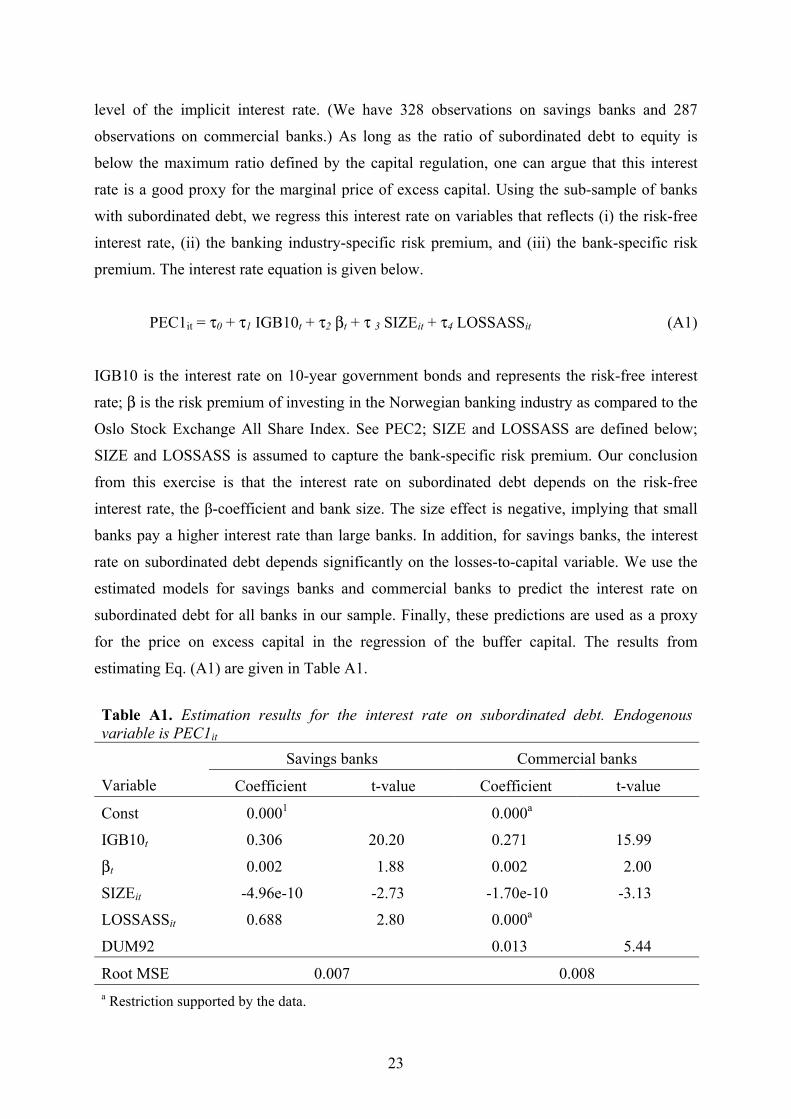
Table A1. Estimation results for the interest rate on subordinated debt. Endogenous variable is PEC1it
Savings banks Commercial banks
Variable Coefficient t-value Coefficient t-value
Const 0.0001 0.000a
IGB10t 0.306 20.20 0.271 15.99
βt 0.002 1.88 0.002 2.00
SIZEit -4.96e-10 -2.73 -1.70e-10 -3.13
LOSSASSit 0.688 2.80 0.000a
DUM92 0.013 5.44
Root MSE 0.007 0.008 a Restriction supported by the data.
24
PEC2: This is the β-coefficient, calculated in accordance with the Sharpe-Lintner capital asset
pricing model (CAPM), as a proxy. See Sharpe (1964) and Lintner (1965). Not all banks are
listed on Oslo Børs (Oslo Stock Exchange), however, and the trading in the hybrid capital
instrument of savings banks is in general relatively small. We, therefore, calculate the β-
coefficient for the Norwegian banking industry and use this common risk premium measure
as a proxy for the price on excess capital. We use the following formula to calculate the β-
coefficient on a quarterly basis9:
βt=Cov[RB , RM]t/Var[RM]t, (A2)
where RB is the daily return on the bank index at Oslo Børs and RM is the daily return on the
Oslo Børs All Share Index. Both RB and RM are return indices where it is assumed that
dividends are reinvested.
VPROF is the variance of each bank’s profit calculated on past observations.
CBUF is the competitors’ average capital buffer. We split the banks into two groups, i.e.
savings banks and commercial bank.
SUP represents supervisory scrutiny. Two alternative measures are applied: (i) SUP(N) is the
number of employees at the beginning of each year at the Norwegian Banking, Insurance and
Securities Commission (BISC). (ii) SUP(I) is the annual number of on-site inspections by
BISC divided by four. The results are robust to the choice of empirical variable, and we
present the results with SUP(I) in the paper.
GDPG denotes the four quarter growth rate of Mainland-Norway’s gross domestic product,
i.e. excluding oil, natural gas and shipping. Measured in per cent.
SIZE is total financial assets incl. guarantees and represents bank size.
USLP is unspecified loan loss provisions relative to risk-weighted assets.
9 Help from Johannes Skjeltorp with the calculations is highly appreciated.
25
TREND is a simple deterministic trend variable. LOSSASS is the previous four quarter moving average of losses relative to capital. Qj, j=2, 3, 4, are quarterly dummy variables that are one in quarter j and zero elsewhere.
Table A2 and A3 give the correlation matrix of the variables used in the regressions for
savings banks and commercial banks respectively. All variables are on logarithmic form. The
largest correlation coefficients between the explanatory variables are found for savings banks
between size and vprof and cbuf and trend, i.e. between bank size and the variance of
cumulative profits and between competitors’ average buffer and the trend. In addition, for
both bank groups, we find some correlation coefficients in the range 0.4-0.5, which may cause
some problems with multicollinearity.

26
Table A2. The correlation matrix of the variables used in the regression, savings banksa
bufit pec2t vprofi,t-1 riskit cbuft-1 supt gdpgt sizeit uslpi,t-1 trendt
bufit 1.000
Pec2t 0.042 1.000
vprofi,t-1 -0.285 -0.016 1.000
riskit 0.160 0.053 -0.161 1.000
cbufk,t-1 0.178 0.247 -0.003 -0.161 1.000
supt 0.001 -0.038 0.015 -0.007 -0.018 1.000
gdpgt 0.117 0.123 -0.013 0.084 0.536 -0.208 1.000
sizeit -0.357 -0.041 0.810 -0.166 -0.111 0.037 -0.071 1.000
uslpi,t-1 0.011 -0.070 0.158 0.133 -0.174 0.022 -0.100 0.205 1.000
trendt -0.187 -0.207 -0.001 -0.198 -0.935 0.039 -0.471 0.118 0.186 1.000 a The variables are on logarithmic form. Based on 3101 observations.
Table A3. The correlation matrix of the variables used in the regression, commercial banksa
bufit pec2t vprofi,t-1 riskit cbuft-1 supt gdpgt sizeit uslpi,t-1 trendt
bufit 1.000
Pec2t -0.018 1.000
vprofi,t-1 -0.279 -0.006 1.000
riskit 0.023 0.120 -0.234 1.000
cbufk,t-1 -0.279 0.265 -0.021 0.097 1.000
supt 0.115 -0.042 -0.023 -0.075 0.466 1.000
gdpgt -0.153 0.123 -0.013 0.138 0.007 -0.199 1.000
sizeit -0.382 -0.032 0.406 -0.185 0.036 0.026 -0.005 1.000
uslpi,t-1 -0.322 0.058 -0.149 0.330 0.037 -0.041 0.064 0.344 1.000
trendt 0.248 -0.189 0.032 -0.244 -0.315 -0.005 -0.465 -0.076 -0.067 1.000 a The variables are on logarithmic form. Based on 300 observations.

27
References
Andreeva, O., 2003. Aggregate bankruptcy probabilities and their role in explaining banks’
loan losses. Forthcoming as Working Paper, Norges Bank.
Ayuso, J., Pérez, D., Saurina, J., 2002. Are Capital Buffers Pro-Cyclical? Evidence from
Spanish panel data. Documento de Trabajo n.° 0224, Banco de España.
Barrios, V.E., Blanco, J.M., 2003. The effectiveness of bank capital adequacy regulation: A
theoretical and empirical approach. Journal of Banking and Finance 27, 1935-1958.
Basel Committee on Banking Supervision, 2001. Review of Procyclicality. Research Task
Force, Mimeo.
Berger, A.N., Herring, R.J., Szegö, G.P., 1995. The Role of Capital in Financial Institutions.
Journal of Banking and Finance 19, 393-430.
Bernhardsen, E., 2001. A model of bankruptcy prediction. Working Paper 2001/10, Norges
Bank.
Borio, C., Furfine, C., Lowe, P., 2001. Procyclicality of the Financial System and Financial
Stability: Issue and Policy Options. BIS papers 1, 1-57.
Boyd, J.H., Gertler, M., 1994. Are Banks Dead? Or Are the Reports Greatly Exaggerated?.
Federal Reserve Bank of Minneapolis Quarterly Review 18, Vol. 3.
Breusch, T., Pagan, A., 1980. The Lagrange multiplier test and its applications to model
specification in econometrics. Review of Economic Studies 47, 239-253.
Danielsson, J., Embrechts, P., Goodhart, C., Keating, C., Muennich, F., Renault, O., Shin,
H.S., 2001. An Academic Response to Basel II. Special Paper 130, Financial Market Group,
London School of Economics.
European Central Bank, 2001. The New Capital Adequacy Regime – the ECB Perspective.
ECB Monthly Bulletin May, 59-74.

28
Freixas, X., Rochet, J.-C., 1997. Microeconomics of Banking. MIT Press, Cambridge.
Furfine, C., 2001. Bank Portfolio Allocation: The Impact of Capital Requirements,
Regulatory Monitoring, and Economic Conditions. Journal of Financial Services Research 20,
33-56.
Hausman, J.A., 1978. Specification tests in econometrics. Econometrica 46, 1251-1271.
Hellwig, M., 1991. Banking, financial intermediation and corporate finance. In Giovannini,
A., Mayer, C. (Eds.), European Financial Integration. Cambridge: Cambridge University
Press.
Hughes, J.P., Mester, L.J., Moon, C.-G, 2000. Are scale economies in banking elusive or
illusive? : evidence obtained by incorporating capital structure and risk-taking into models of
bank production. Working Paper No. 00-4, Federal Reserve Bank of Philadelphia.
Kim, D., Santomero, A.M., 1988. Risk in Banking and Capital Regulation. Journal of Finance
43, 1219-1233.
Kim, M., Kristiansen, E.G., Vale, B., 2001. Endogenous product differentiation in credit
markets: What do borrowers pay for?. Working Paper 2001/08, Norges Bank.
Koehn, M., Santomero, A.M., 1980. Regulation of Bank Capital and Portfolio Risk. Journal
of Finance 35, 1235-1244.
Lintner, J., 1965. The Valuation of Risky Assets and the Selection of Risky Investments in
Stock Portfolios and Capital Budgets. Review of Economics and Statistics 47, 13-37.
Reidhill, J. (Ed.), 2003. Bank Failures in Mature Economies. Working Paper, forthcoming,
Basel Committee on Banking Supervision.
Rochet, J.-C., 1992a. Capital Requirements and the Behaviour of Commercial Banks.
European Economic Review 36, 1137-1170.

29
Rochet, J.-C., 1992b. Towards a Theory of Optimal Banking Regulation. Cahiers
Economiques et Monétaires de la Banque de France 40, 275-284.
Santos, J.A.C., 2000. Bank Capital Regulation in Contemporary Banking Theory: A Review
of the Literature. Financial Markets, Institutions and Instruments 10, 41-84.
Sharpe, W., 1964. Capital Asset Prices: A Theory of Market Equilibrium under Conditions of
Risk. Journal of Finance 19, 425-442.
StataCorp, 2001. Stata Statistical Software: Release 7.0. College Station, TX: Stata
Corporation.
Stortinget, 1998. Rapport til Stortinget fra kommisjonen som ble nedsatt av Stortinget for å
gjennomgå ulike årsaksforhold knyttet til bankkrisen. Dokument nr. 7 (1997-98).
Steigum, E. (2002): Financial Deregulation with a Fixed Exchange Rate: Lessons from
Norway’s Boom – Bust Cycle and Banking Crisis. BI draft paper.

30
WORKING PAPERS (ANO) FROM NORGES BANK 2002-2003 Working Papers were previously issued as Arbeidsnotater from Norges Bank, see Norges Bank’s website http://www.norges-bank.no
2002/1 Bache, Ida Wolden Empirical Modelling of Norwegian Import Prices Research Department 2002, 44p
2002/2 Bårdsen, Gunnar og Ragnar Nymoen Rente og inflasjon Forskningsavdelingen 2002, 24s
2002/3 Rakkestad, Ketil Johan Estimering av indikatorer for volatilitet Avdeling for Verdipapirer og internasjonal finans Norges Bank 33s
2002/4 Akram, Qaisar Farooq PPP in the medium run despite oil shocks: The case of Norway Research Department 2002, 34p
2002/5 Bårdsen, Gunnar, Eilev S. Jansen og Ragnar Nymoen Testing the New Keynesian Phillips curve Research Department 2002, 38p
2002/6 Lindquist, Kjersti-Gro The Effect of New Technology in Payment Services on Banks’Intermediation Research Department 2002, 28p
2002/7 Sparrman, Victoria Kan pengepolitikken påvirke koordineringsgraden i lønnsdannelsen? En empirisk analyse. Forskningsavdelingen 2002, 44s
2002/8 Holden, Steinar The costs of price stability - downward nominal wage rigidity in Europe Research Department 2002, 43p
2002/9 Leitemo, Kai and Ingunn Lønning Simple Monetary Policymaking without the Output Gap Research Department 2002, 29p
2002/10 Leitemo, Kai Inflation Targeting Rules: History-Dependent or Forward-Looking? Research Department 2002, 12p
2002/11 Claussen, Carl Andreas Persistent inefficient redistribution International Department 2002, 19p
2002/12 Næs, Randi and Johannes A. Skjeltorp Equity Trading by Institutional Investors: Evidence on Order Submission Strategies Research Department 2002, 51p
2002/13 Syrdal, Stig Arild A Study of Implied Risk-Neutral Density Functions in the Norwegian Option Market Securities Markets and International Finance Department 2002, 104p

31
2002/14 Holden, Steinar and John C. Driscoll A Note on Inflation Persistence Research Department 2002, 12p
2002/15 Driscoll, John C. and Steinar Holden Coordination, Fair Treatment and Inflation Persistence Research Department 2002, 40p
2003/1 Erlandsen, Solveig Age structure effects and consumption in Norway, 1968(3) – 1998(4) Research Department 2003, 27p
2003/2 Bakke, Bjørn og Asbjørn Enge Risiko i det norske betalingssystemet Avdeling for finansiell infrastruktur og betalingssystemer 2003, 15s
2003/3 Matsen, Egil and Ragnar Torvik Optimal Dutch Disease Research Department 2003, 26p
2003/4 Bache, Ida Wolden Critical Realism and Econometrics Research Department 2002, 18p
2003/5 David B. Humphrey and Bent Vale Scale economies, bank mergers, and electronic payments: A spline function approach
Research Department 2003, 34p
2003/6 Harald Moen Nåverdien av statens investeringer i og støtte til norske banker
Avdeling for finansiell analyse og struktur 2003, 24s
2003/7 Geir H. Bjønnes, Dagfinn Rime and Haakon O.Aa. Solheim Volume and volatility in the FX market: Does it matter who you are?
Research Department 2003, 24p
2003/8 Olaf Gresvik and Grete Øwre Costs and Income in the Norwegian Payment System 2001. An application of the Activity Based Costing framework
Financial Infrastructure and Payment Systems Department 2003, 51p
2003/9 Randi Næs and Johannes A.Skjeltorp Volume Strategic Investor Behaviour and the Volume-Volatility Relation in Equity Markets
Research Department 2003, 43p
2003/10 Geir Høidal Bjønnes and Dagfinn Rime Dealer Behavior and Trading Systems in Foreign Exchange Markets¤ Research Department 2003, 32p
2003/11 Kjersti-Gro Lindquist Banks’ buffer capital: How important is risk Research Department 2003, 31p

Kjersti-Gro Lindquist: Banks’ buffer capital: How im
portant is risk?W
orking Paper 2003/11
KEYWORDS:
BankingExcess capitalRiskPanel data
- 16912