bank of japan working paper · pdf filewhen making a copy or reproduction, the source, bank...
TRANSCRIPT

Empirical Evidence on “Systemic as a Herd”:
The Case of Japanese Regional Banks
Naohisa Hirakata* [email protected]
Yosuke Kido* [email protected]
Jie Liang Thum** [email protected]
No.17-E-1 January 2017
Bank of Japan 2-1-1 Nihonbashi-Hongokucho, Chuo-ku, Tokyo 103-0021, Japan
* Financial System and Bank Examination Department, Bank of Japan ** Monetary Authority of Singapore
Papers in the Bank of Japan Working Paper Series are circulated in order to stimulate discussion and comments. Views expressed are those of authors and do not necessarily reflect those of the Bank. If you have any comment or question on the working paper series, please contact each author. When making a copy or reproduction of the content for commercial purposes, please contact the Public Relations Department ([email protected]) at the Bank in advance to request permission. When making a copy or reproduction, the source, Bank of Japan Working Paper Series, should explicitly be credited.
Bank of Japan Working Paper Series

1
Empirical Evidence on "Systemic as a Herd":
The Case of Japanese Regional Banks
Naohisa Hirakata*, Yosuke Kido†, and Jie Liang Thum‡
January 2017
Abstract
We examine a sample of Japanese regional banks and explore whether exposure to market risk factors affects systemic risk through a banks’ portfolio composition or revenue source, using Adrian and Brunnermeier’s (2016) CoVaR to proxy for systemic risk. We find evidence of “systemic as a herd” behavior among Japanese regional banks, as portfolio and revenue components associated with market activities exert positive and significant impacts on systemic risk by generating higher comovement among banks, even though they reduce standalone bank risk through portfolio diversification. Further, the marginal effect of an increase in a given banks’ market-related components on systemic risk is larger when the share of the corresponding components is already high among other banks. Our results have important implications from the macro-prudential perspective.
JEL classification: D21; G28; G32; G38; G62
Keywords: Systemic risk; Herd behavior; Market risk factors; CoVaR
* Financial System and Bank Examination Department, Bank of Japan (E-mail: [email protected]). † Financial System and Bank Examination Department, Bank of Japan (E-mail: [email protected]). ‡ Monetary Authority of Singapore (E-mail: [email protected]).
We are grateful for the helpful comments from Hibiki Ichiue, Takeshi Kimura, Yoshihiro Komaki, Hitoshi Mio, and staff of the Bank of Japan. The views expressed herein are those of the authors alone and do not necessarily reflect those of the Bank of Japan or the Monetary Authority of Singapore.
2
1. Introduction
Systemic banking crises tend to be costly, with costs often exceeding that imposed
by individual bank failures. Therefore, more attention is being paid to forestalling
systemic crises and mitigating their impact. As opposed to the question of
“too-big-to-fail”, which has attracted much scrutiny, the problem of “systemic as a
herd”, whereby institutions which are not individually systemically important behave in
a similar way and are thus exposed to common risks, has attracted relatively less
attention. However, “systemic as a herd” behavior increases the probability of joint
failure among herding institutions and thus can have financial stability implications. In
this paper, we investigate “systemic as a herd” behavior, specifically, the effect of
portfolio and revenue source diversification on both systemic and standalone bank risk.
The question of how financial institutions' portfolio composition or revenue source
affects standalone bank risk is a topic of active research. Stiroh (2004, 2006) concludes
that greater reliance on non-interest income, particularly trading revenue, is associated
with higher risk across commercial banks.1 Other research finds support, albeit limited
to hypothetical scenarios, for the risk reduction benefits of diversification. Employing
simulated mergers between banks and non-bank financial firms, Laderman (2000) finds
that diversification into insurance activities could reduce the variation in return on assets
and also banks’ probability of bankruptcy. By constructing synthetic portfolios between
1981 and 1989, Wall, Reichert and Mohanty (1993) find that banks could enjoy higher
returns and lower risk, by diversifying to a small extent into non-banking activities.
While previous research sheds light on the implications of portfolio composition or
revenue structure for individual banks, research on its systemic risk implications is
limited.2 One way in which banks’ portfolio composition or revenue structure could
affect systemic risk is through exposure to common factors, such as market fluctuations.
If banks are similarly exposed to market-related factors through their portfolio
1 DeYoung and Roland (2001) present similar findings. 2 For example, Brunnermeier, Dong and Palia (2012) examine the effect of non-traditional, non-interest income activities on systemic risk, and report that non-interest income components make a larger contribution compared to traditional banking activities, such as lending.
3
composition or revenue structure, these common exposures increase the risk that many
banks could fail together and lead to a system-wide problem.3
In this paper, we investigate the effect of portfolio composition and revenue
structure on both systemic risk and standalone bank risk, employing Japanese regional
bank data. Specifically, we ask whether increased securities holdings and reliance on
non-interest income among Japanese regional banks will affect systemic risk and
standalone bank risk. Since securities investments are more likely associated with
common factors, compared with traditional lending activities, higher exposure to
market-related components such as securities investments could render a bank more
correlated with other banks. The higher correlation could result even though regional
banks may not be interconnected directly, through the interbank lending market, for
example. This phenomena is termed “systemic as a herd” in Adrian and Brunnermeier
(2016).4 We use a recently developed measure, Adrian and Brunnermeier (2016)'s
CoVaR to proxy for systemic risk. In this paper, we ask if CoVaR, which captures the
common exposure to exogenous aggregate macroeconomic risk factors, is in agreement
with the idea that Japanese regional banks could be behaving in a manner consistent
with “systemic as a herd”.
The novelty of our paper is twofold. First, previous papers have focused on
interbank exposures or funding structures as a source of systemic risk. While we
3 There are theoretical studies on the effect of portfolio diversification on systemic risk. For example, Acharya and Yorulmazer (2007) coined the term “too-many-to-fail” to describe the situation where a regulator finds it optimal to bail out some or all banks that face bankruptcy as a result of their herd behavior and common exposure to risks. Similarly, Farhi and Tirole (2012) show that if central banks have no choice but to intervene when systemic implications are present, banks will be incentivized to take on more correlated risk. Restating the problem facing an individual bank, it would appear to be “unwise to play safely while everyone else gambles”. Exploring a different transmission channel, Wagner (2010) shows that diversification could lead to increased similarity in banks’ portfolios and expose them to the same risks, which causes a rise in the probability that banks fail simultaneously. 4 The concept of “systemic as a herd” is further clarified below. Consider a case where a large number of small financial institutions are not interconnected directly (e.g. absence of lender and borrower relationships) but are exposed to the same risk factors because they hold similar positions or rely on similar funding sources. Since each financial institution is small, its distressed state or failure may not necessarily trigger a systemic crisis. However, if the source of distress is common to a large number of financial institutions, a common risk event could cause them to enter a distressed state simultaneously. The vulnerability of the entire financial system to a crisis state is thus heightened.

4
acknowledge the importance of those factors, our paper takes a different approach,
exploring how revenue source and portfolio composition can also play a role. To our
knowledge, this is the first paper that documents that the portfolio composition of banks
– namely the securities-to-assets ratio – also has an impact on systemic risk. Second, we
employ data for Japanese regional banks, which are neither considered to be
individually systemically important nor strongly interconnected, but have exhibited a
tendency to increase their securities holdings and non-interest income over time, mainly
due to the decrease in loan demand and profitability. The potential for “systemic as a
herd” behavior is thus present – Japanese regional banks are ideal candidates for testing
the validity and relevance of this concept.
Our main empirical findings are as follows. First, we find that increased securities
holdings or dependence on non-interest income increase our measure of systemic risk
(CoVaR). Further, while these factors reduce standalone bank risk (VaR), a component
of systemic risk, they raise the systemic risk coefficient, a parameter that captures the
linkage between the individual bank's tail risk and aggregated tail risk. This implies that
although increases in securities holdings and non-interest income may not increase
standalone bank risk, it may have the side-effect of rendering the financial system as a
whole more vulnerable. Second, we find that the marginal effects of securities holdings
or dependence on non-interest income on systemic risk depend on other banks' portfolio
composition or revenue structure. Specifically, the more banks increase their reliance on
non-interest income and securities holdings in aggregate, the more an increase in these
factors at a given bank will exert a marginal effect on systemic risk. This implies that
when banks which are not individually systemically important behave in a similar way
and thus exposed to common risk, systemic risk could increase to a greater extent,
compared to the case where such behavior is confined to a limited number of banks.
The remainder of the paper is organized as follows. Section 2 outlines the measure
of systemic risk we use. Section 3 discusses the data, our CoVaR estimation framework
and main results. Section 4 presents an extended model and additional results. Section 5
concludes.
5
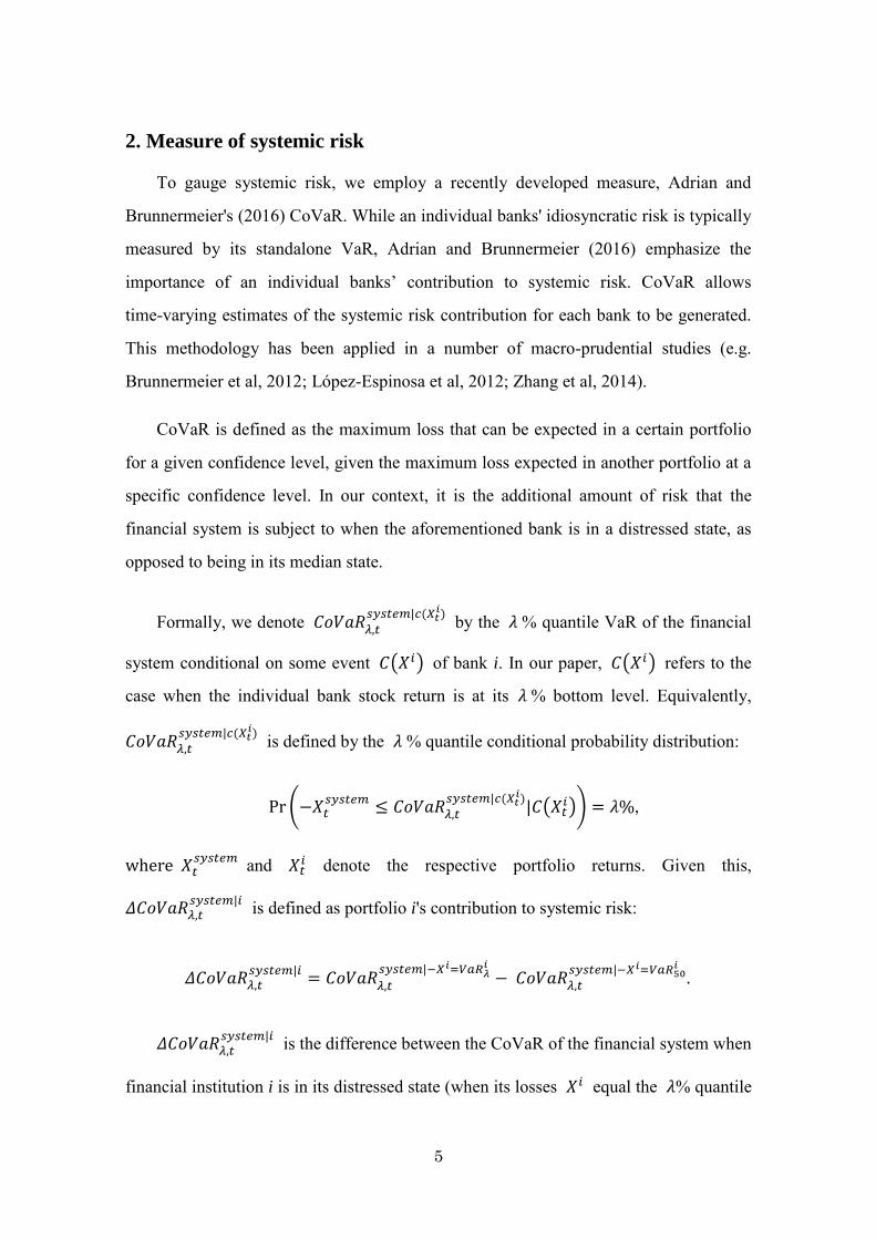
2. Measure of systemic risk
To gauge systemic risk, we employ a recently developed measure, Adrian and
Brunnermeier's (2016) CoVaR. While an individual banks' idiosyncratic risk is typically
measured by its standalone VaR, Adrian and Brunnermeier (2016) emphasize the
importance of an individual banks’ contribution to systemic risk. CoVaR allows
time-varying estimates of the systemic risk contribution for each bank to be generated.
This methodology has been applied in a number of macro-prudential studies (e.g.
Brunnermeier et al, 2012; López-Espinosa et al, 2012; Zhang et al, 2014).
CoVaR is defined as the maximum loss that can be expected in a certain portfolio
for a given confidence level, given the maximum loss expected in another portfolio at a
specific confidence level. In our context, it is the additional amount of risk that the
financial system is subject to when the aforementioned bank is in a distressed state, as
opposed to being in its median state.
Formally, we denote
by the % quantile VaR of the financial
system conditional on some event ( ) of bank i. In our paper, ( ) refers to the
case when the individual bank stock return is at its % bottom level. Equivalently,
is defined by the % quantile conditional probability distribution:
(
(
)) ,
and
denote the respective portfolio returns. Given this,
is defined as portfolio i's contribution to systemic risk:
.
is the difference between the CoVaR of the financial system when
financial institution i is in its distressed state (when its losses equal the % quantile

6
of its VaR), and the CoVaR of the financial system when financial institution i is in its
median state (when its losses equal the 50% quantile of its VaR).
The CoVaR methodology requires the estimation of VaR for individual banks and
any system portfolio in our sample. The key step in the CoVaR methodology is to
estimate the conditional comovement measure. Following Adrian and Brunnermeier
(2016), we compute the predicted value of an aggregate regional bank loss on the loss of
a particular bank i for the 5% quantile. We estimate systemic risk coefficient via
quantile regression, as proposed by Koenker and Bassett (1978). Specifically, we solve
the following equation:
∑{
|
|
|
|
where denotes a state variable. In this expression, the existence of risk
spillover is captured by estimating parameter : for non-zero values of this parameter,
the left tail of the system distribution can be predicted by observing the given
distribution of a bank's returns. Our specification utilizes TOPIX stock returns as a state
variable. Parameters are estimated using daily data with a rolling sample of 126
business days (half-year).
Applying the definition of value at risk, it can be seen that the % quantile of
CoVaR can be computed from the % quantile of bank i VaR. ΔCoVaR is then derived
according to the equation below, by taking the difference between VaR for bank i at the
% quantile and VaR for the same bank in its median state.
( )⏟
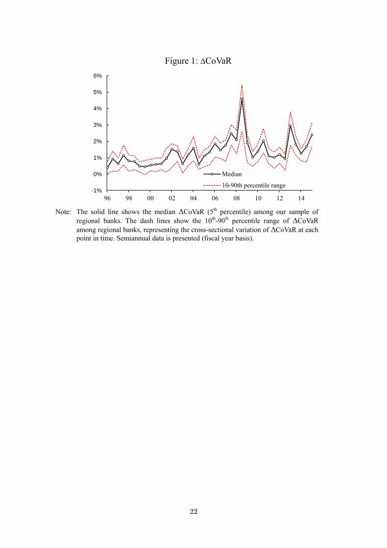
Figure 1 displays the estimated 5% quantile ΔCoVaR of Japanese regional banks in
the sample period April 1996 to March 2016.5 In terms of bank coverage, we selected
5 The sample period is determined based on the availability of bank level data mentioned in Section 3. This sample period is sufficiently long in Japan's case, as it includes the late 1990s banking crisis
7
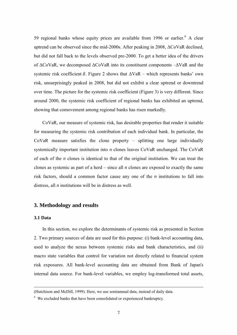
59 regional banks whose equity prices are available from 1996 or earlier.6 A clear
uptrend can be observed since the mid-2000s. After peaking in 2008, ΔCoVaR declined,
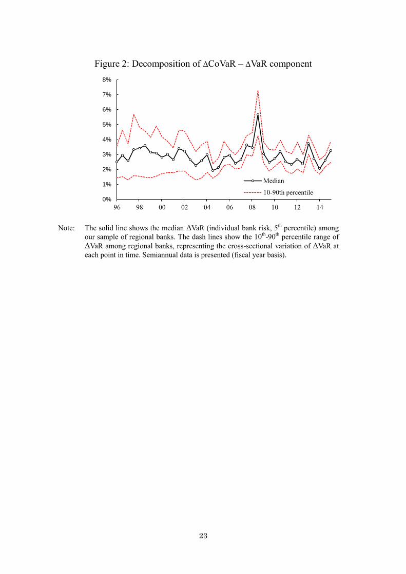
but did not fall back to the levels observed pre-2000. To get a better idea of the drivers
of ΔCoVaR, we decomposed ΔCoVaR into its constituent components –ΔVaR and the
systemic risk coefficient . Figure 2 shows that ΔVaR – which represents banks’ own
risk, unsurprisingly peaked in 2008, but did not exhibit a clear uptrend or downtrend
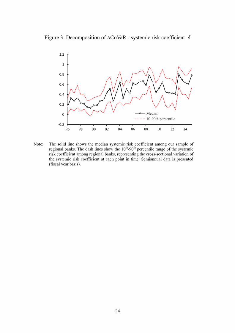
over time. The picture for the systemic risk coefficient (Figure 3) is very different. Since
around 2000, the systemic risk coefficient of regional banks has exhibited an uptrend,
showing that comovement among regional banks has risen markedly.
CoVaR, our measure of systemic risk, has desirable properties that render it suitable
for measuring the systemic risk contribution of each individual bank. In particular, the
CoVaR measure satisfies the clone property – splitting one large individually
systemically important institution into n clones leaves CoVaR unchanged. The CoVaR
of each of the n clones is identical to that of the original institution. We can treat the
clones as systemic as part of a herd – since all n clones are exposed to exactly the same
risk factors, should a common factor cause any one of the n institutions to fall into
distress, all n institutions will be in distress as well.
3. Methodology and results
3.1 Data
In this section, we explore the determinants of systemic risk as presented in Section
2. Two primary sources of data are used for this purpose: (i) bank-level accounting data,
used to analyze the nexus between systemic risks and bank characteristics, and (ii)
macro state variables that control for variation not directly related to financial system
risk exposures. All bank-level accounting data are obtained from Bank of Japan's
internal data source. For bank-level variables, we employ log-transformed total assets,
(Hutchison and McDill, 1999). Here, we use semiannual data, instead of daily data. 6 We excluded banks that have been consolidated or experienced bankruptcy.
8
which captures bank size ( ), securities-to-assets ( ), loans-to-assets
( ) and the non-interest income-to-income ratio ( ), which represent banks’
balance sheet and revenue source exposures.7
The loans-to-assets ratio shows how reliant a bank is on traditional lending
activities. In the case of Japanese regional banks, loans are largely extended to
households or firms in the operating area of the bank, and thus the loans-to-assets ratio
represents a risk factor more attributable to a specific bank. The securities-to-assets ratio
is a measure of a bank’s exposure to market risk factors, which may be driven by
common factors.8 The non-interest income-to-interest income ratio is a proxy for the
extent to which a bank is reliant on non-traditional activities, such as fees and
commissions income related to investment trusts, relative to traditional deposit and
lending activities.
As for macro state variables, we employ Japanese stock market volatility9 (30-day
historical volatility of the TOPIX index); the Japanese yen “TED spread” (i.e. 3-month
Yen LIBOR less 3-month JGB yields); excess return of the real estate sector over the
financial sector (using TOPIX subsector returns); TOPIX returns; 3-month JGB yields;
and the term spread (10-year JGB yields less 3-month JGB yields), following Adrian
and Brunnermeier (2016). All data are measured as semiannual averages, except for
3-month JGB yields and the term spread, where the first difference in semiannual
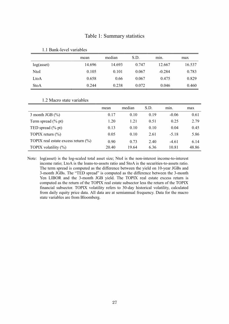
averages is employed. Table 1 presents summary statistics of the data employed.
7 Other potential variables of interest include non-core liabilities, which is often linked to financial system vulnerability (Shin, 2011). However, this variable does not suit our empirical exercise as deposits form a very large share of funding for our sample banks. 8 Acharya and Yorulmazer (2007) consider a two asset model comprising a bank-specific asset and a common asset. In our empirical analysis, loans, which comprise banks’ main portfolio, are considered to be more bank-specific, while securities are considered to have more common asset characteristics. 9 While Adrian and Brunnermeier (2016) employ implied volatility calculated from options prices, due to data limitations, we employ historical stock return volatility computed with daily data instead.
9
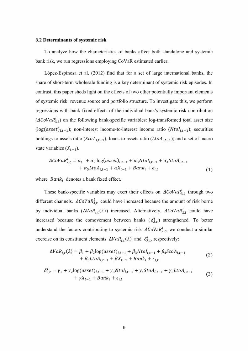
3.2 Determinants of systemic risk
To analyze how the characteristics of banks affect both standalone and systemic
bank risk, we run regressions employing CoVaR estimated earlier.
López-Espinosa et al. (2012) find that for a set of large international banks, the
share of short-term wholesale funding is a key determinant of systemic risk episodes. In
contrast, this paper sheds light on the effects of two other potentially important elements
of systemic risk: revenue source and portfolio structure. To investigate this, we perform
regressions with bank fixed effects of the individual bank's systemic risk contribution
( ) on the following bank-specific variables: log-transformed total asset size
( ); non-interest income-to-interest income ratio ( ); securities
holdings-to-assets ratio ( ); loans-to-assets ratio ( ); and a set of macro
state variables ( ).
where denotes a bank fixed effect.
These bank-specific variables may exert their effects on through two
different channels. could have increased because the amount of risk borne
by individual banks ( ) increased. Alternatively, could have
increased because the comovement between banks ( ) strengthened. To better
understand the factors contributing to systemic risk , we conduct a similar
exercise on its constituent elements and , respectively:
10
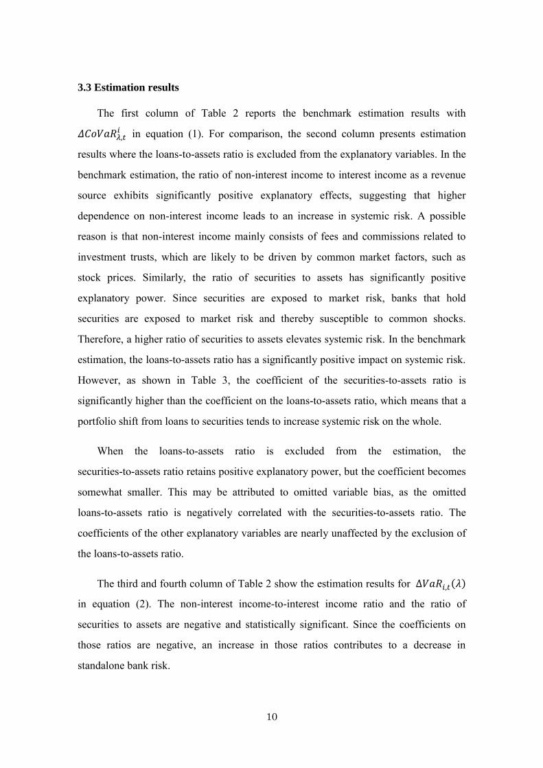
3.3 Estimation results
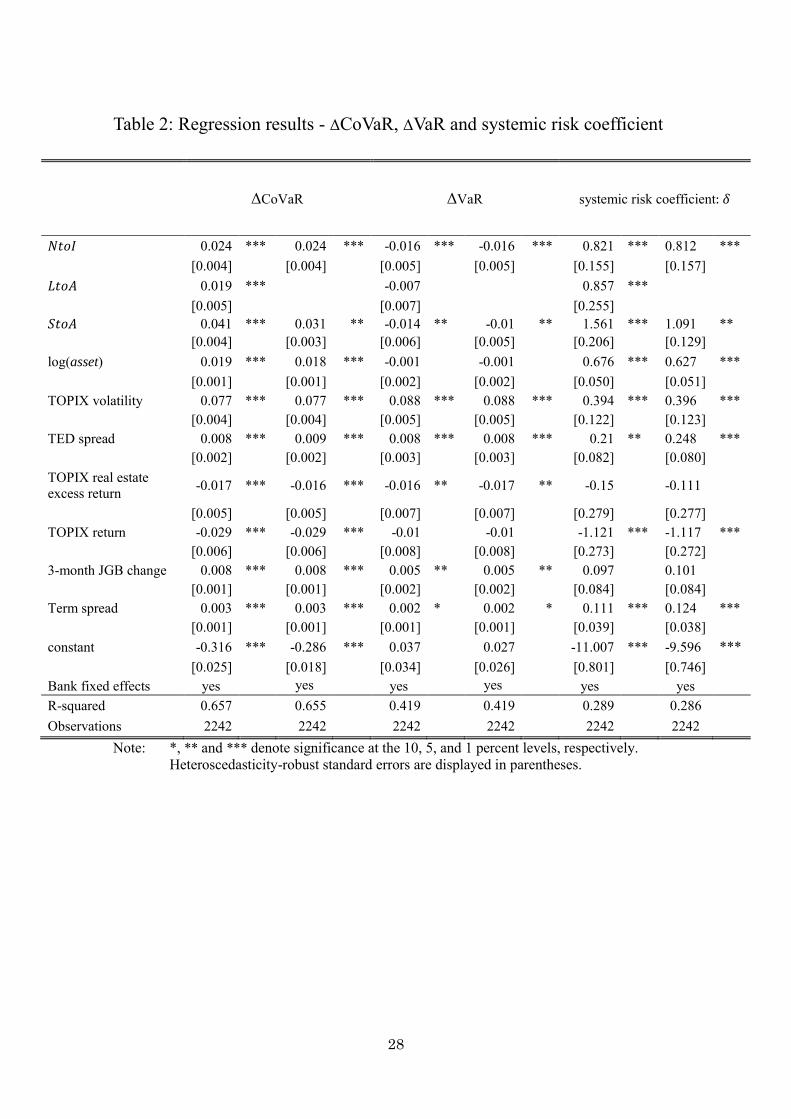
The first column of Table 2 reports the benchmark estimation results with
in equation (1). For comparison, the second column presents estimation
results where the loans-to-assets ratio is excluded from the explanatory variables. In the
benchmark estimation, the ratio of non-interest income to interest income as a revenue
source exhibits significantly positive explanatory effects, suggesting that higher
dependence on non-interest income leads to an increase in systemic risk. A possible
reason is that non-interest income mainly consists of fees and commissions related to
investment trusts, which are likely to be driven by common market factors, such as
stock prices. Similarly, the ratio of securities to assets has significantly positive
explanatory power. Since securities are exposed to market risk, banks that hold
securities are exposed to market risk and thereby susceptible to common shocks.
Therefore, a higher ratio of securities to assets elevates systemic risk. In the benchmark
estimation, the loans-to-assets ratio has a significantly positive impact on systemic risk.
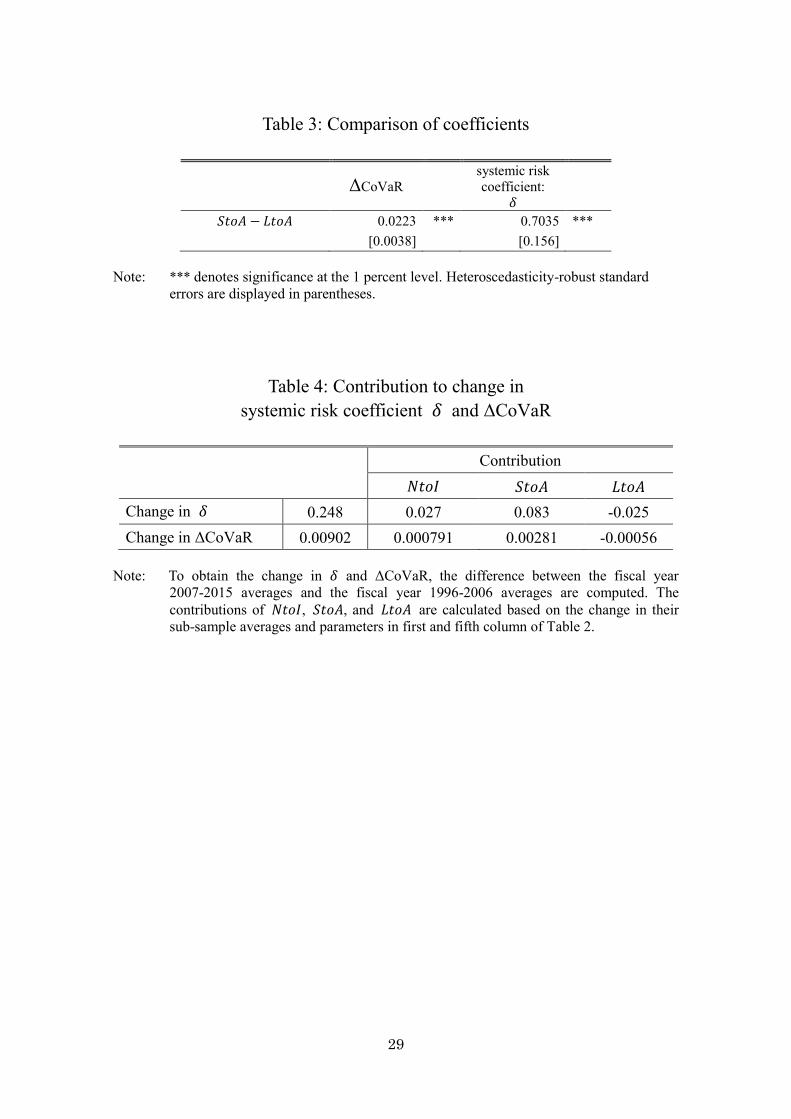
However, as shown in Table 3, the coefficient of the securities-to-assets ratio is
significantly higher than the coefficient on the loans-to-assets ratio, which means that a
portfolio shift from loans to securities tends to increase systemic risk on the whole.
When the loans-to-assets ratio is excluded from the estimation, the
securities-to-assets ratio retains positive explanatory power, but the coefficient becomes
somewhat smaller. This may be attributed to omitted variable bias, as the omitted
loans-to-assets ratio is negatively correlated with the securities-to-assets ratio. The
coefficients of the other explanatory variables are nearly unaffected by the exclusion of
the loans-to-assets ratio.
The third and fourth column of Table 2 show the estimation results for
in equation (2). The non-interest income-to-interest income ratio and the ratio of
securities to assets are negative and statistically significant. Since the coefficients on
those ratios are negative, an increase in those ratios contributes to a decrease in
standalone bank risk.
11
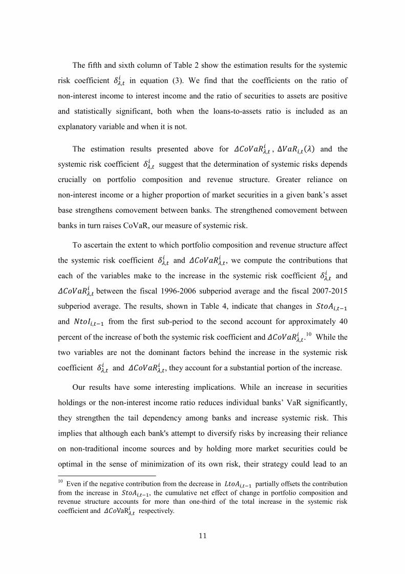
The fifth and sixth column of Table 2 show the estimation results for the systemic
risk coefficient in equation (3). We find that the coefficients on the ratio of
non-interest income to interest income and the ratio of securities to assets are positive
and statistically significant, both when the loans-to-assets ratio is included as an
explanatory variable and when it is not.
The estimation results presented above for , and the
systemic risk coefficient suggest that the determination of systemic risks depends
crucially on portfolio composition and revenue structure. Greater reliance on
non-interest income or a higher proportion of market securities in a given bank’s asset
base strengthens comovement between banks. The strengthened comovement between
banks in turn raises CoVaR, our measure of systemic risk.
To ascertain the extent to which portfolio composition and revenue structure affect
the systemic risk coefficient and
, we compute the contributions that
each of the variables make to the increase in the systemic risk coefficient and
between the fiscal 1996-2006 subperiod average and the fiscal 2007-2015
subperiod average. The results, shown in Table 4, indicate that changes in
and from the first sub-period to the second account for approximately 40
percent of the increase of both the systemic risk coefficient and .10 While the
two variables are not the dominant factors behind the increase in the systemic risk
coefficient and
, they account for a substantial portion of the increase.
Our results have some interesting implications. While an increase in securities
holdings or the non-interest income ratio reduces individual banks’ VaR significantly,
they strengthen the tail dependency among banks and increase systemic risk. This
implies that although each bank's attempt to diversify risks by increasing their reliance
on non-traditional income sources and by holding more market securities could be
optimal in the sense of minimization of its own risk, their strategy could lead to an 10 Even if the negative contribution from the decrease in partially offsets the contribution from the increase in , the cumulative net effect of change in portfolio composition and revenue structure accounts for more than one-third of the total increase in the systemic risk coefficient and R
respectively.
12
unintended increase in the level of systemic risk. Our results could therefore be
capturing the idea that individual banks are behaving "systemic as a herd”. These results
are consistent with Wagner (2010), which shows that even though diversification in
income source and portfolio composition pursued by each financial institution reduces
each institution's individual probability of failure, it makes systemic crises more likely.
Overall, it suggests that business activities associated with market risk should be
assessed more stringently from the macro-prudential perspective, because such activities
can raise systemic risk, which entails a negative externality.
4. Extended model
The previous section confirmed that exposure to common risk factors present in
securities holdings or non-interest income raise systemic risk by strengthening the
comovement between banks, not by raising standalone bank risk, at least in the sample
period examined. However, the same result – that systemic risk increases when the
exposure of individual banks to market-related factors grows – may not hold generally.
It is possible to conceive a situation where the comovement between a given bank and
other banks in the financial system falls. For example, if a given bank increases its
securities holdings or non-interest income ratio in a situation where the
securities-to-assets ratio or non-interest income-to-interest income ratio among the
majority of banks in the financial system is limited, the revenue or profit structure of the
bank in question could become more dissimilar to that of other banks. Conversely, if
those ratios among the majority of banks are already high, an increase in securities
holdings or reliance on non-interest income could strengthen comovement between
banks and thus raise systemic risk. The effect on systemic risk of a change in portfolio
composition or revenue structure at a given bank thus depends on the portfolio
composition and revenue structure at other banks. To analyze this, this section presents
a simple model and the results of additional empirical exercises.

13
4.1 A simple model of comovement
Consider two banks, Bank i and Bank j, which are conducting two different
activities. The first activity they engage in is market-related activity, which includes
investments in securities and commission-based non-interest income. The other activity
is traditional loans, which generates interest income. Earnings from those activities at
period t are denoted by and , respectively. It is assumed that these activities are
governed by hierarchical-factor models:
√
,
√
,
where denotes a market factor that both banks are exposed to, denotes a
loan factor that both banks share, and and denote correlation coefficients
whose absolute values are no more than 1. Both factors are linked by the underlying
macro-factor :
,
.
In the above, and are uncorrelated idiosyncratic factors for the market
factor and the loan factor, and and
are uncorrelated idiosyncratic factors
inherent in Bank i's market related activities and loan activities respectively. Bank i's
income and Bank j's income are given by:
( ) ,
( )
and are Bank i and j 's weights on market-related activities, respectively.
The covariance between and is obtained as follows:
( ) ( ) ( ),
14
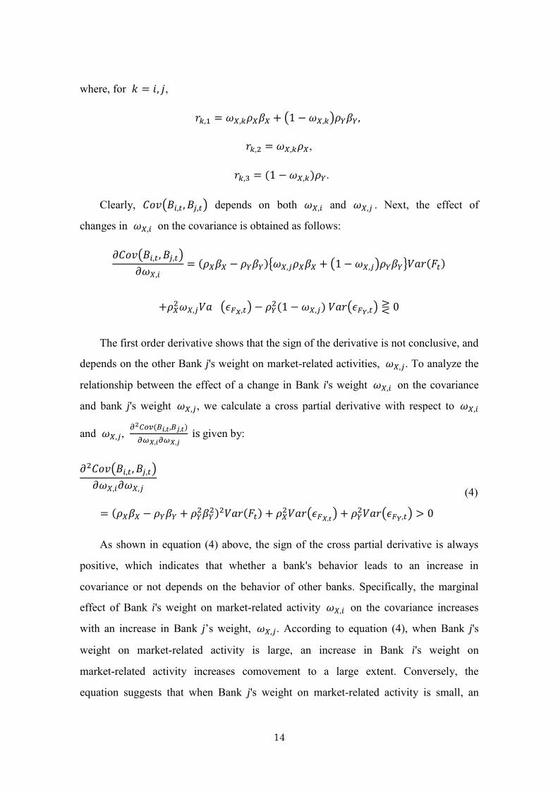
where, for ,
( )
,
.
Clearly, ( ) depends on both and . Next, the effect of
changes in on the covariance is obtained as follows:
( )
{ ( ) }
�( )
( )
The first order derivative shows that the sign of the derivative is not conclusive, and
depends on the other Bank j's weight on market-related activities, . To analyze the
relationship between the effect of a change in Bank i's weight on the covariance
and bank j's weight , we calculate a cross partial derivative with respect to
and ,
given by:
( )
(
) ( )
(4)
As shown in equation (4) above, the sign of the cross partial derivative is always
positive, which indicates that whether a bank's behavior leads to an increase in
covariance or not depends on the behavior of other banks. Specifically, the marginal
effect of Bank i's weight on market-related activity on the covariance increases
with an increase in Bank j’s weight, . According to equation (4), when Bank j's
weight on market-related activity is large, an increase in Bank i's weight on
market-related activity increases comovement to a large extent. Conversely, the
equation suggests that when Bank j's weight on market-related activity is small, an
15
increase in Bank i's market-related activity can lead to a smaller covariance. In this case,
the increase in Bank i's weight on increases the compositional difference between
the two banks’ portfolios, which leads to diversification in the financial system as a
whole.
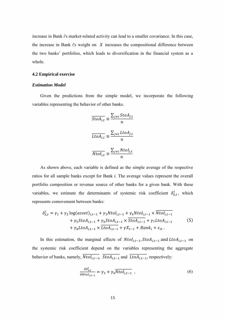
4.2 Empirical exercise
Estimation Model
Given the predictions from the simple model, we incorporate the following
variables representing the behavior of other banks.
∑
∑
∑
As shown above, each variable is defined as the simple average of the respective
ratios for all sample banks except for Bank i. The average values represent the overall
portfolio composition or revenue source of other banks for a given bank. With these
variables, we estimate the determinants of systemic risk coefficient , which
represents comovement between banks:
In this estimation, the marginal effects of on
the systemic risk coefficient depend on the variables representing the aggregate
behavior of banks, namely, and , respectively:
, (6)
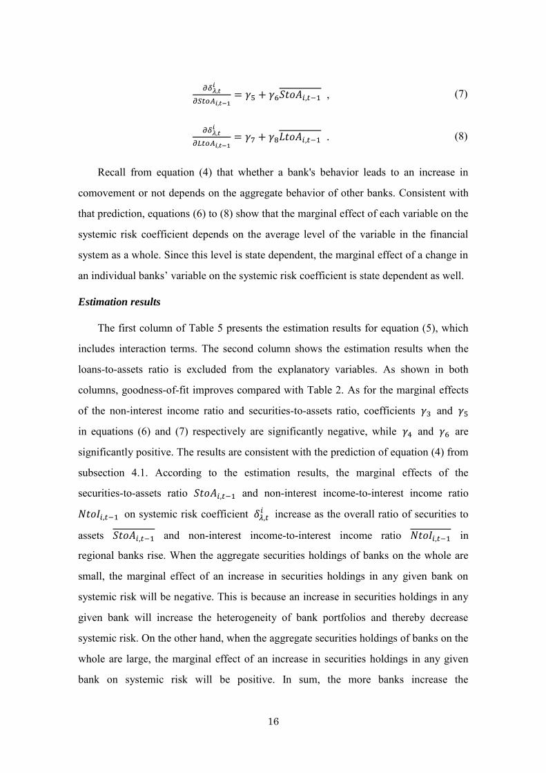
16
, (7)
. (8)
Recall from equation (4) that whether a bank's behavior leads to an increase in
comovement or not depends on the aggregate behavior of other banks. Consistent with
that prediction, equations (6) to (8) show that the marginal effect of each variable on the
systemic risk coefficient depends on the average level of the variable in the financial
system as a whole. Since this level is state dependent, the marginal effect of a change in
an individual banks’ variable on the systemic risk coefficient is state dependent as well.
Estimation results
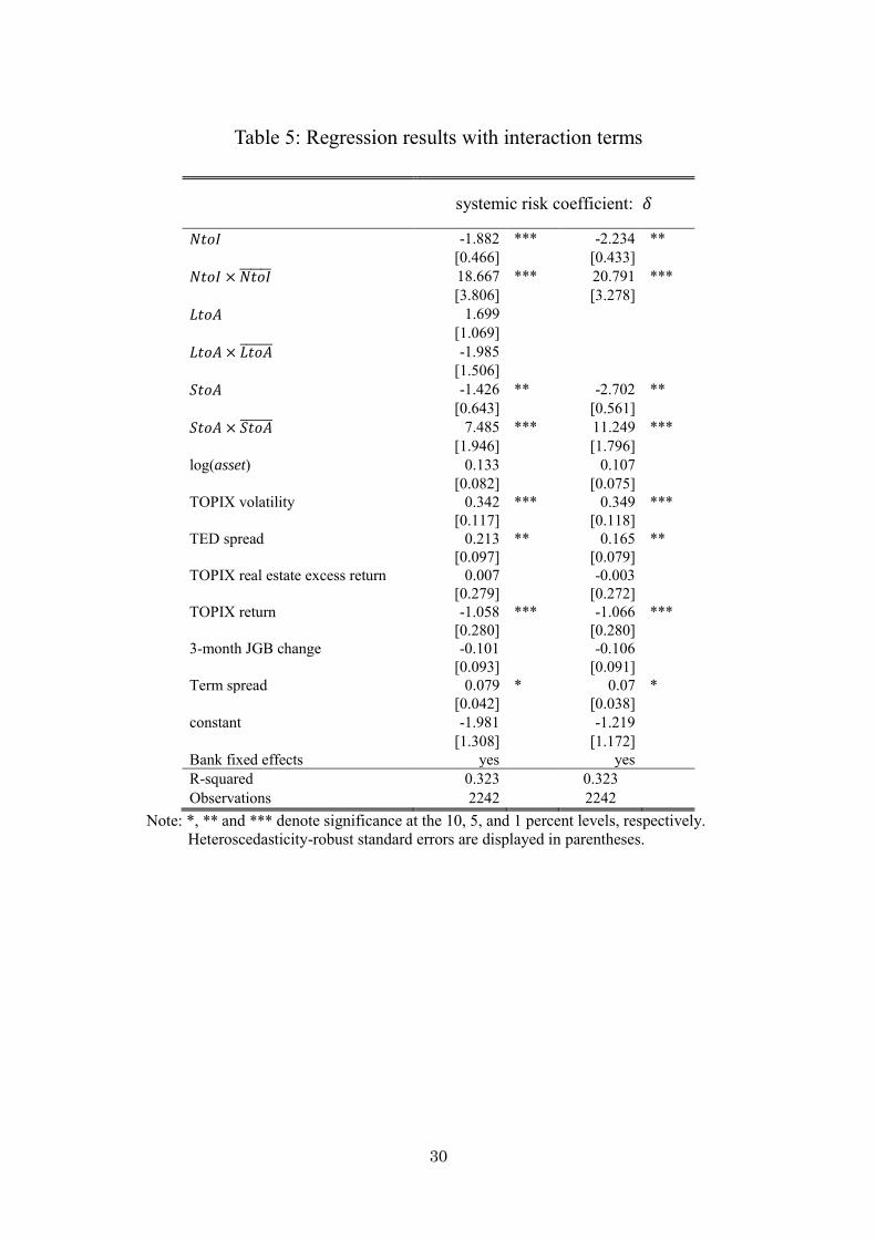
The first column of Table 5 presents the estimation results for equation (5), which
includes interaction terms. The second column shows the estimation results when the
loans-to-assets ratio is excluded from the explanatory variables. As shown in both
columns, goodness-of-fit improves compared with Table 2. As for the marginal effects
of the non-interest income ratio and securities-to-assets ratio, coefficients and
in equations (6) and (7) respectively are significantly negative, while and are
significantly positive. The results are consistent with the prediction of equation (4) from
subsection 4.1. According to the estimation results, the marginal effects of the
securities-to-assets ratio and non-interest income-to-interest income ratio
on systemic risk coefficient increase as the overall ratio of securities to
assets and non-interest income-to-interest income ratio in
regional banks rise. When the aggregate securities holdings of banks on the whole are
small, the marginal effect of an increase in securities holdings in any given bank on
systemic risk will be negative. This is because an increase in securities holdings in any
given bank will increase the heterogeneity of bank portfolios and thereby decrease
systemic risk. On the other hand, when the aggregate securities holdings of banks on the
whole are large, the marginal effect of an increase in securities holdings in any given
bank on systemic risk will be positive. In sum, the more banks increase the
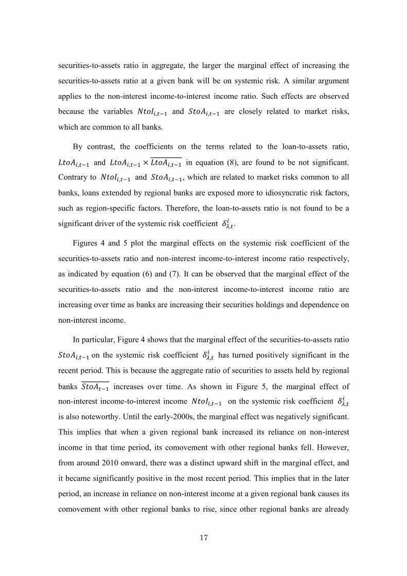
17
securities-to-assets ratio in aggregate, the larger the marginal effect of increasing the
securities-to-assets ratio at a given bank will be on systemic risk. A similar argument
applies to the non-interest income-to-interest income ratio. Such effects are observed
because the variables and are closely related to market risks,
which are common to all banks.
By contrast, the coefficients on the terms related to the loan-to-assets ratio,
and in equation (8), are found to be not significant.
Contrary to and , which are related to market risks common to all
banks, loans extended by regional banks are exposed more to idiosyncratic risk factors,
such as region-specific factors. Therefore, the loan-to-assets ratio is not found to be a
significant driver of the systemic risk coefficient .
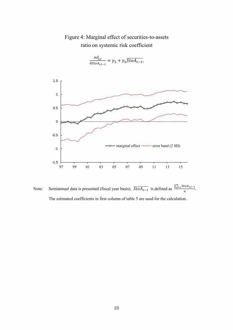
Figures 4 and 5 plot the marginal effects on the systemic risk coefficient of the
securities-to-assets ratio and non-interest income-to-interest income ratio respectively,
as indicated by equation (6) and (7). It can be observed that the marginal effect of the
securities-to-assets ratio and the non-interest income-to-interest income ratio are
increasing over time as banks are increasing their securities holdings and dependence on
non-interest income.
In particular, Figure 4 shows that the marginal effect of the securities-to-assets ratio
on the systemic risk coefficient has turned positively significant in the
recent period. This is because the aggregate ratio of securities to assets held by regional
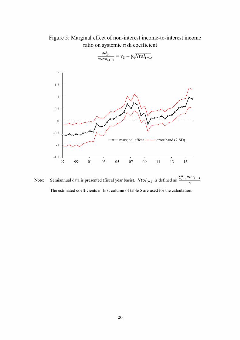
banks increases over time. As shown in Figure 5, the marginal effect of
non-interest income-to-interest income on the systemic risk coefficient
is also noteworthy. Until the early-2000s, the marginal effect was negatively significant.
This implies that when a given regional bank increased its reliance on non-interest
income in that time period, its comovement with other regional banks fell. However,
from around 2010 onward, there was a distinct upward shift in the marginal effect, and
it became significantly positive in the most recent period. This implies that in the later
period, an increase in reliance on non-interest income at a given regional bank causes its
comovement with other regional banks to rise, since other regional banks are already

18
highly reliant on non-interest income, rendering their revenue source more exposed to a
common factor.
As stated above, we obtain empirical findings that are consistent with the
predictions of the model presented earlier in this section. That is, systemic risk could
increase when a bank's exposure to common factors, such as market risk, increases. In
particular, systemic risk could increase to a greater extent when other banks’ exposure
to the same common factors is already high.
5. Conclusion
As banks hold a larger share of securities and shift toward non-traditional sources
of income, namely non-interest income, standalone bank risk may be lowered through
portfolio diversification, although systemic risk may increase through reduced diversity
among banks. In this paper, we ask if there is evidence that individual banks pursue
diversification of their own portfolios and revenue sources, producing at the same time
the unintended side effect of increased exposure to common risks.
By examining the relationship between a measure of systemic risk, CoVaR, and the
income sources and portfolio compositions for a set of Japanese regional banks, we find
that increased exposure of bank portfolios to market risks and greater reliance on
non-traditional income sources associated with market activities raise systemic risk,
even though they reduce standalone bank risk. Further, we find that the marginal effect
of an increase in a given banks’ market-related components on systemic risk is larger
when the share of the corresponding components is already high among other banks.
Although regional banks are individually non-systemic, they have the potential to
behave “systemic as a herd”, whereby common shocks generate losses across distinct
financial institutions with similar portfolio holdings, and cause these financial
institutions to respond in a similar manner. It should be noted that the adverse effect of
diversification in our paper does not originate from contagion through interbank
linkages – whether or not a bank fails does not depend on direct exposure to other banks.

19
Rather, the common shock is transmitted through comovements in asset holdings and
income sources.
Our paper is an empirical complement to theory on the potential costs and limits
of diversification (Wagner, 2010). It suggests that contrary to common belief, it is not
desirable for banks to pursue diversification to the maximum extent possible, since
“systemic as a herd” behavior could increase the vulnerability of the financial system.
From a macro-prudential perspective, it is essential to address the externality
associated with greater vulnerability to joint failure stemming from “systemic as a herd”
behavior. For example, Goodhart and Wagner (2012) suggest introducing a surcharge
on existing capital requirements depending on how correlated their overall activities are
with the rest of the financial system. Alternatively, current risk weights could be
redefined to penalize activities that are more exposed to common risk factors, while
keeping average capital requirements unchanged. Such policies may render banks that
have more potential for “systemic as a herd” behavior less risky, since they will be
made to hold more capital.
20
References
Acharya, V. and T. Yorulmazer (2007) “Too Many to Fail—An Analysis of Time-inconsistency in Bank Closure Policies,” Journal of Financial Intermediation, Vol. 16, pp. 1–31. Adrian, T., and M. K. Brunnermeier (2016) “CoVaR,” American Economic Review, Vol. 106(7), pp. 1705-41. Brunnermeier, M. K., G. Dong and D. Palia (2012) “Banks’ Non-Interest Income and Systemic Risk,” AFA 2012 Chicago Meetings Paper. DeYoung, R. and K. P. Roland, (2001) "Product Mix and Earnings Volatility at Commercial Banks: Evidence from a Degree of Total Leverage Model," Journal of
Financial Intermediation, Vol. 10(1), pp. 54-84. Farhi E. and J. Tirole (2012) “Collective Moral Hazard, Maturity Mismatch, and Systemic Bailouts,” American Economic Review, Vol. 102(1), pp.60–93. Goodhart,C. and W. Wagner (2012) “Regulators Should Encourage More Diversity in the Financial System” http://voxeu.org/article/regulators-should-encourage-more-diversity-financial-system Hutchison, M. and K. McDill (1999) “Are All Banking Crises Alike? The Japanese Experience in International Comparison,” Journal of the Japanese and International
Economies, Vol. 13(3), pp. 155-180. Koenker, R., and G. Bassett Jr (1978) “Regression Quantiles,” Econometrica, Vol. 46(1), pp. 33-50. Laderman, E. S. (2000) “The Potential Diversification and Failure Reduction Benefits of Bank Expansion into Nonbanking Activities,” Federal Reserve Bank of San
Francisco Working Paper Series 2000-01. López-Espinosa, G., A. Moreno, A. Rubia and L. Valderrama (2012) “Short-term Wholesale Funding and Systemic Risk: A Global CoVaR Approach,” Journal of
Banking & Finance, Vol. 36(12), pp. 3150-3162.
21
Shin, H. S. (2011). Macroprudential policies beyond Basel III. BIS Papers, 1, 5. Stiroh, K. J. (2004) “Diversification in Banking: Is Noninterest Income the Answer?” Journal of Money, Credit and Banking, Vol. 36(5), pp. 853-882. Stiroh, K. J. (2006) “A Portfolio View of Banking with Interest and Noninterest Activities,” Journal of Money, Credit and Banking, Vol. 38(5), pp. 1351-1361. Wagner, W. (2010) “Diversification at Financial Institutions and Systemic Crises,” Journal of Financial Intermediation, Vol. 19, pp. 373-386. Wall, L. D., A. K. Reichert and S. Mohanty (1993) “Deregulation and the Opportunities for Commercial Bank Diversification,” Federal Reserve Bank of Atlanta, Economic
Review, September/October, pp. 1-25. Zhang, Q., F. Vallascas, K. Keasey and C. X. Cai (2014) “Are Market-based Rankings of Global Systemic Importance of Financial Institutions Useful to Regulators and Supervisors?” Journal of Money, Credit, and Banking, Vol. 47(7), pp. 1403-1442.
22
Figure 1: ΔCoVaR
Note: The solid line shows the median ΔCoVaR (5th percentile) among our sample of
regional banks. The dash lines show the 10th-90th percentile range of ΔCoVaR among regional banks, representing the cross-sectional variation of ΔCoVaR at each point in time. Semiannual data is presented (fiscal year basis).
-1%
0%
1%
2%
3%
4%
5%
6%
96 98 00 02 04 06 08 10 12 14
Median
10-90th percentile range
23
Figure 2: Decomposition of ΔCoVaR – ΔVaR component
Note: The solid line shows the median ΔVaR (individual bank risk, 5th percentile) among our sample of regional banks. The dash lines show the 10th-90th percentile range of ΔVaR among regional banks, representing the cross-sectional variation of ΔVaR at each point in time. Semiannual data is presented (fiscal year basis).
0%
1%
2%
3%
4%
5%
6%
7%
8%
96 98 00 02 04 06 08 10 12 14
Median
10-90th percentile
24
Figure 3: Decomposition of ΔCoVaR - systemic risk coefficient
Note: The solid line shows the median systemic risk coefficient among our sample of regional banks. The dash lines show the 10th-90th percentile range of the systemic risk coefficient among regional banks, representing the cross-sectional variation of the systemic risk coefficient at each point in time. Semiannual data is presented (fiscal year basis).
-0.2
0
0.2
0.4
0.6
0.8
1
1.2
96 98 00 02 04 06 08 10 12 14
Median10-90th percentile
25
Figure 4: Marginal effect of securities-to-assets ratio on systemic risk coefficient
,
Note: Semiannual data is presented (fiscal year basis). is defined as
∑
.
The estimated coefficients in first column of table 5 are used for the calculation.
-1.5
-1
-0.5
0
0.5
1
1.5
97 99 01 03 05 07 09 11 13 15
marginal effect error band (2 SD)
26
Figure 5: Marginal effect of non-interest income-to-interest income ratio on systemic risk coefficient
,
Note: Semiannual data is presented (fiscal year basis). is defined as
∑
.
The estimated coefficients in first column of table 5 are used for the calculation.
-1.5
-1
-0.5
0
0.5
1
1.5
2
97 99 01 03 05 07 09 11 13 15
marginal effect error band (2 SD)
27
Table 1: Summary statistics
1.1 Bank-level variables
mean median S.D. min. max
log(asset) 14.696 14.693 0.747 12.667 16.537 NtoI 0.105 0.101 0.067 -0.284 0.783 LtoA 0.658 0.66 0.067 0.475 0.829 StoA 0.244 0.238 0.072 0.046 0.460
1.2 Macro state variables
mean median S.D. min. max 3 month JGB (%) 0.17 0.10 0.19 -0.06 0.61 Term spread (% pt) 1.20 1.21 0.51 0.25 2.79 TED spread (% pt) 0.13 0.10 0.10 0.04 0.45 TOPIX return (%) 0.05 0.10 2.61 -5.18 5.86 TOPIX real estate excess return (%) 0.90 0.73 2.40 -4.61 6.14 TOPIX volatility (%) 20.40 19.64 6.36 10.81 48.86
Note: log(asset) is the log-scaled total asset size; NtoI is the non-interest income-to-interest
income ratio; LtoA is the loans-to-assets ratio and StoA is the securities-to-assets ratio. The term spread is computed as the difference between the yield on 10-year JGBs and 3-month JGBs. The “TED spread” is computed as the difference between the 3-month Yen LIBOR and the 3-month JGB yield. The TOPIX real estate excess return is computed as the return of the TOPIX real estate subsector less the return of the TOPIX financial subsector. TOPIX volatility refers to 30-day historical volatility, calculated from daily equity price data. All data are at semiannual frequency. Data for the macro state variables are from Bloomberg.
28
Table 2: Regression results - ΔCoVaR, ΔVaR and systemic risk coefficient
ΔCoVaR ΔVaR systemic risk coefficient
0.024 *** 0.024 *** -0.016 *** -0.016 *** 0.821 *** 0.812 ***
[0.004] [0.004] [0.005] [0.005] [0.155] [0.157]
0.019 *** -0.007 0.857 *** [0.005] [0.007] [0.255] 0.041 *** 0.031 ** -0.014 ** -0.01 ** 1.561 *** 1.091 **
[0.004] [0.003] [0.006] [0.005] [0.206] [0.129] log(asset) 0.019 *** 0.018 *** -0.001 -0.001 0.676 *** 0.627 ***
[0.001] [0.001] [0.002] [0.002] [0.050] [0.051] TOPIX volatility 0.077 *** 0.077 *** 0.088 *** 0.088 *** 0.394 *** 0.396 ***
[0.004] [0.004] [0.005] [0.005] [0.122] [0.123] TED spread 0.008 *** 0.009 *** 0.008 *** 0.008 *** 0.21 ** 0.248 ***
[0.002] [0.002] [0.003] [0.003] [0.082] [0.080] TOPIX real estate excess return -0.017 *** -0.016 *** -0.016 ** -0.017 ** -0.15 -0.111
[0.005] [0.005] [0.007] [0.007] [0.279] [0.277] TOPIX return -0.029 *** -0.029 *** -0.01 -0.01 -1.121 *** -1.117 ***
[0.006] [0.006] [0.008] [0.008] [0.273] [0.272] 3-month JGB change 0.008 *** 0.008 *** 0.005 ** 0.005 ** 0.097 0.101
[0.001] [0.001] [0.002] [0.002] [0.084] [0.084] Term spread 0.003 *** 0.003 *** 0.002 * 0.002 * 0.111 *** 0.124 ***
[0.001] [0.001] [0.001] [0.001] [0.039] [0.038] constant -0.316 *** -0.286 *** 0.037 0.027 -11.007 *** -9.596 ***
[0.025] [0.018] [0.034] [0.026] [0.801] [0.746] Bank fixed effects yes yes yes yes yes yes R-squared 0.657 0.655 0.419 0.419 0.289 0.286 Observations 2242 2242 2242 2242 2242 2242
Note: *, ** and *** denote significance at the 10, 5, and 1 percent levels, respectively. Heteroscedasticity-robust standard errors are displayed in parentheses.
29
Table 3: Comparison of coefficients
ΔCoVaR systemic risk coefficient:
0.0223 *** 0.7035 ***
[0.0038] [0.156]
Note: *** denotes significance at the 1 percent level. Heteroscedasticity-robust standard
errors are displayed in parentheses.
Table 4: Contribution to change in systemic risk coefficient and ΔCoVaR
Contribution
Change in 0.248 0.027 0.083 -0.025 Change in ΔCoVaR 0.00902 0.000791 0.00281 -0.00056
Note: To obtain the change in and ΔCoVaR, the difference between the fiscal year
2007-2015 averages and the fiscal year 1996-2006 averages are computed. The contributions of , , and are calculated based on the change in their sub-sample averages and parameters in first and fifth column of Table 2.
30
Table 5: Regression results with interaction terms
systemic risk coefficient:
-1.882 *** -2.234 **
[0.466] [0.433] 18.667 *** 20.791 ***
[3.806] [3.278] 1.699
[1.069] -1.985
[1.506] -1.426 ** -2.702 **
[0.643] [0.561] 7.485 *** 11.249 ***
[1.946] [1.796] log(asset) 0.133 0.107
[0.082] [0.075]
TOPIX volatility 0.342 *** 0.349 ***
[0.117] [0.118]
TED spread 0.213 ** 0.165 **
[0.097] [0.079]
TOPIX real estate excess return 0.007 -0.003
[0.279] [0.272]
TOPIX return -1.058 *** -1.066 ***
[0.280] [0.280]
3-month JGB change -0.101 -0.106
[0.093] [0.091]
Term spread 0.079 * 0.07 *
[0.042] [0.038]
constant -1.981 -1.219
[1.308] [1.172]
Bank fixed effects yes yes R-squared 0.323 0.323 Observations 2242 2242
Note: *, ** and *** denote significance at the 10, 5, and 1 percent levels, respectively. Heteroscedasticity-robust standard errors are displayed in parentheses.