Bank Mergers and Crime:The Real and Social Effects of Credit Market Competition

Mark J. Garmaise and Tobias J. Moskowitz∗

ABSTRACT

Using a unique sample of commercial loans and mergers between large banks, we provide micro-level(within-county) evidence linking credit conditions to economic development and find a spillover ef-fect on crime. Neighborhoods that experienced more bank mergers are subjected to higher interestrates, diminished local construction, lower prices, an influx of poorer households, and higher prop-erty crime in subsequent years. The elasticity of property crime with respect to merger-inducedbanking concentration is 0.18. We show that these results are not likely due to reverse causa-tion, and confirm the central findings using state branching deregulation to instrument for bankcompetition.

∗Garmaise is from the UCLA Anderson School and Moskowitz is from the Graduate School of Business, University of

Chicago and NBER. We have benefitted from the suggestions and comments of Tony Bernardo, Marianne Bertrand,

Phillip Bond, Doug Diamond, Mark Duggan, Eugene Fama, Kenneth French, Jonathan Guryan, Erik Hurst, Matthias

Kahl, Anil Kashyap, Steven Levitt, Atif Mian, Sendhil Mullainathan, Canice Prendergast, Raghu Rajan, Tano Santos,

Per Stromberg, Luigi Zingales, and seminar participants at the University of Chicago Graduate School of Business,

NYU, Wharton, UCLA, University of Washington, and Dartmouth College. Special thanks to Michael Arabe, John

Edkins, and Peggy McNamara as well as COMPS.com for providing the U.S. commercial real estate data, to Bob

Figlio, Dave Ingeneri, and CAP Index, Inc. for providing the crime data, to F.W. Dodge Division of the McGraw-Hill

Companies, Inc. for providing the construction data, to John J. Donohue III and Steven Levitt for providing abortion

rate and imprisonment rate data, and to Phil Strahan for providing state bank branching dates. Moskowitz thanks

the Center for Research in Security Prices and the James S. Kemper Foundation Research Fund for financial support.

Correspondence to: Tobias Moskowitz, Graduate School of Business, University of Chicago, 1101 E. 58th St.,

Chicago, IL 60637. E-mail: tobias.moskowitz@gsb.uchicago.edu.

We examine the real and social impact of local credit competition by documenting a link between

the competitiveness of the local banking market, credit conditions, urban development, and crime.

Several recent studies (Peek and Rosengren (2000), Cetorelli and Gambera (2001), Klein, Peek, and

Rosengren (2002), and Burgess and Pande (2003)) tie credit market imperfections to diminished

real economic activity and growth. Other studies connect the economic environment to property

crime (Freeman (1999), Levitt (2001), Raphael and Winter-Ebmer (2001), and Nilsson (2004)). It

is reasonable to hypothesize, therefore, that reductions in bank competition may lead to economic

decline and, subsequently, increases in property crime. We empirically investigate the effects of

bank consolidation and increased market power on credit availability and real activity using a

unique sample of commercial loans and mergers between large banks in the 1990’s. We provide

micro-level evidence that neighborhoods that experienced greater reductions in bank competition

due to bank mergers are subjected to future higher interest rates, diminished local construction,

lower real estate prices, and an influx of poorer households. We then examine whether these changes

impact the social environment by studying subsequent changes in crime rates across neighborhoods,

and find an associated increase in property crime. Importantly, these results do not appear to be

due to reverse causation since, among other evidence, our large bank mergers are not preceded by

or contemporaneously correlated with crime increases or economic declines.

Our empirical strategy considers only neighborhood (within county) variation in bank loan

market competitiveness induced by mergers between non-failing banks of at least $1 billion in

assets to capture plausibly exogenous changes in the competitiveness of local banking markets.

The size, scope, and health of these banks makes it unlikely that economic declines in the local

neighborhoods we examine are driving the mergers. We then analyze the local market effects

of these mergers on subsequent loan supply, interest rates, property prices, investment activity,

economic and demographic variables, and crime. It is worth emphasizing at the outset that we

only examine the relation between changes in bank competition through large mergers and changes

in economic conditions and crime across neighborhoods. Bank competition cannot explain the

aggregate national decline in crime over the last few decades nor differences in the level of crime

across regions. Indeed, we control for both the time trend and variation in crime levels across

counties in our analysis.

Local financial development can be critical to economic growth even in a well-integrated financial

environment (Guiso, Sapienza, and Zingales (2004)). The market for small commercial real estate

1

loans is localized due to information and agency considerations (Garmaise and Moskowitz (2003,

2004)). For these reasons, merger-induced changes in the local competitive environment can have

sizeable effects. We find that when loan competition declines (via large bank mergers), interest

rates charged on loans rise significantly and borrowers receive smaller loans.1 Using bank-specific

fixed effects, we show that the same bank is setting different loan terms in areas with different levels

of competition. It is important to note, however, that these mergers lead to short-term distortions

in the loan market. In the longer-term, entry of new banks and increased loan supply by existing

banks should lead to a restored competitive equilibrium (Berger, et al. (1998)). Consistent with

this notion, we show that mergers’ impact on the local competitive environment lasts about three

years, ceasing to have any significant effect beyond that time.

It is during this short-term distortion of the local loan market that large banking mergers have

substantial real economic implications. We find that commercial real estate development, which is

often a marginal investment for banks, and new construction activity fall significantly. In addition,

local property prices decline. Examining local demographic and migration data from the census,

we then find that unemployment in the area rises, median income drops, and income inequality

increases. Moreover, the income of new arrivals into the neighborhood is below that of long-term

residents, suggesting an influx of lower income households into the area.

These changing economic and demographic characteristics provide a plausible channel through

which crime may rise. In particular, we find subsequent increases in burglary and, more broadly,

property crimes in these areas. There appears to be, however, no significant increase in homicide

or other personal crimes, which have a tenuous relation with economic activity. It is a general

conclusion of the crime literature that economic decline is linked closely to property crime but

loosely, if at all, to personal/violent crime (see Levitt (2001), Raphael and Winter-Ebmer (2001),

and Nilsson (2004)). Our results are consistent with bank mergers leading to economic deterioration,

which in turn results in more property crime, but has no definite effect on violent crime. We find

that the elasticity of property crime risk with respect to merger-induced bank concentration is 0.18.

The crime literature reports elasticities of crime with respect to direct economic variables such as

wages and unemployment in the range of 0.6 to 0.9, (Grogger (1998), Rickman and Witt (2003)),

so the magnitude of the elasticity we find suggests an indirect effect of credit market terms on

property crime via economic mechanisms. The effect on crime itself is small, but clearly important

to local residents. Applying our results to national crime figures from the FBI’s Uniform Crime

2

Reports, a mean decline in banking competitiveness due to mergers from 1992 to 1995 is associated

with approximately 24,300 more property crime offenses over the period 1995 to 2000.

We also find that the differential effect of mergers on property crime risks varies across neigh-

borhoods. Areas that already have high banking concentration and low median income are more

severely affected by a merger-induced reduction in loan competition. This suggests that the real

and social costs of bank mergers can be much higher in fragile neighborhoods.

While we believe that this body of evidence suggests a plausible causal (though indirect) link

from bank mergers to crime, a natural alternative theory for these results is reverse causation.

In considering the hypothesis that future crime increases are in some way prompting present-day

mergers, we first note that commercial real estate loans are only a small part of banks’ portfolios

and, in any case, the future price effects we find correlated with mergers are small. In addition, we

consider only the mergers of non-failing, very large banks, which almost certainly are not driven by

the possibility of future neighborhood-level declines. Nonetheless, we investigate the hypothesis that

some unobservable economic variables affecting future crime motivate present-day bank mergers.

Evidence against this alternative hypothesis is summarized in the following set of results. First,

we find that while bank mergers antedate economic deterioration and increases in crime, economic

decline and increases in crime are not correlated with either contemporary or future bank mergers.

Second, while we employ only non-failing banks for our merger variable, as a robustness test we

also compute a change in concentration measure from the mergers of failing banks only, since

these are the most likely to be associated with economic declines in the neighborhoods in which

they operate. We find, however, that mergers between failing banks do not predict future crime

increases. While difficult to reconcile with reverse causation, this finding is consistent with mergers

affecting competition, since the removal of a failing bank from the market probably has only a

small competitive effect. Third, we also examine changes in the number of non-lending financial

institutions such as insurance companies and securities brokers. These institutions, like banks,

are affected by the current and past local economic environment, but unlike banks they should

have little impact on local credit conditions. Consistent with this, we find no association between

consolidation of non-lending institutions and future crime, failing to support reverse causation.

Finally, when we consider mergers that should not affect the local competitive environment, for

example when outsider banks acquire insider banks or mergers within the same bank holding

company, such mergers do not predict changes in credit conditions or increases in future crime.

3

This collection of results suggests the reverse causation theory is not very plausible.

Although we focus on neighborhood variation in economic activity and crime, we also examine

county and state level variation to obtain additional construction and crime statistics and show

that increased bank mergers predict reduced construction activity and higher burglary rates, but

again do not predict homicide rates. At the state level, we also employ another measure of bank

competition using variation in state deregulation of bank branching. Branching deregulation had

the opposite effect of mergers by improving credit competition. In years immediately following

deregulation of branching restrictions within a state, we find decreases in banking concentration,

loan rate reduction, increasing loan sizes, rising property prices, and declining burglary rates, with

no effect on homicide. These findings further support the link between credit conditions, economic

activity, and property crime.

Our findings relate to the literature on the real effects of credit market imperfections.2 They

are also broadly consistent with the literature on finance and development.3 Complementing this

literature, we provide micro-level evidence of neighborhood credit markets within the U.S. having

important impacts on local real activity. We further provide novel evidence on spillovers from credit

market competitiveness to social outcomes such as crime. More broadly, the potential connection

between finance, real, and social activity is an intriguing area of further study.

The rest of the paper is organized as follows. Section I details the commercial loan, crime,

construction, census, and bank merger data used to examine the real and social effects of financial

access. Section II describes our empirical strategy to exogenously measure changes in banking

competitiveness through large bank mergers. Section III analyzes the impact of bank competition

changes (through mergers) on subsequent loan supply, economic and demographic variables, and

crime risks. Section IV provides further evidence on the exogeneity of the bank merger variable

and tests alternative theories such as reverse causation. Section V conducts county and state level

analysis employing state deregulation of bank branching as another instrument for competition.

Finally, Section VI concludes the paper.

4

I. Data and Summary Statistics

We briefly describe the variety of data sources used in the paper.

A. Transaction level data from the U.S. commercial real estate market

Our sample consists of 22,642 commercial real estate transactions drawn from across the U.S.

over the period January 1, 1992 to March 30, 1999 from COMPS.com, a leading provider of

commercial real estate sales data. Garmaise and Moskowitz (2003a, 2003b) provide an extensive

description of the COMPS database and detailed summary statistics. The data span 11 states:

California, Nevada, Oregon, Massachusetts, Maryland, Virginia, Texas, Georgia, New York, Illinois,

and Colorado, plus the District of Columbia.

Properties are grouped into three mutually exclusive types: Apartments (defined as multi-family

dwellings, apartment complexes, condominiums, and townhouses), vacant land, and commercial and

industrial buildings. Panel A of Table I reports summary statistics on the properties in our sample.

The average (median) sale price is $2.4 million ($600,000), and there are only 42 transactions

involving REITS (less than 0.2% of the sample). Capitalization rates, defined as net income on the

property divided by sale price, and property age are also reported.

[***Insert Table I here***]

The COMPS database provides detailed information about specific property transactions, in-

cluding location, identity and location of market participants, and financial structure. For example,

COMPS provides eight digit latitude and longitude coordinates of the property’s location (accurate

to within 10 meters). From these, we construct characteristics of the local market in which each

property resides by matching each property with local crime risks and census statistics.

A.1 Financial structure and terms

The COMPS data contain detailed financing information for each property transaction. We

focus on the terms of the loan contract, including interest rates, and the size and presence of loans.

As Panel A of Table I indicates, the average loan size (from bank and non-bank institutions) as

a fraction of sale price is over 75%. The data also contain rich detail on loan terms including the

annual interest rate, the maturity of the loan, whether the loan rate is floating or fixed, whether

amortized and the length of amortization, and whether the loan was subsidized by the Small

Business Administration (only 1.3% of loans).

5

Panel B of Table I describes the subset of loans that are made by identifiable banks (for some

loans the source is not identified and other loans are made by insurance companies, investment

banks, or other financial institutions). We identify 769 distinct banks making loans in our sample.

Of these, we classify 210 “large banks” as those having at least $1 billion in assets. It is the mergers

among these large banks that we employ as our instrument for competition. Large banks made

5,092 loans, comprising 60% of the total number of loans, but tended to make larger loans on

average, comprising more than 74% of debt financings on a dollar basis.

B. Bank merger activity

Since we employ mergers between large banks as an instrument for changes in bank competition

in the local area (discussed in detail in the next section), we report summary statistics on bank

merger and acquisition activity over our sample period in Panel B of Table I. Information on bank

mergers is obtained from the Commercial Bank Database of the Federal Reserve. Information on

bank high holding companies (used to track asset levels and acquisitions) is obtained from the Call

Report Database (Reports of Condition and Income data) of the Federal Reserve System, Federal

Deposit Insurance Corporation, and the Comptroller of the Currency.

We include only the following types of mergers and acquisitions in our study:

(i). Bank mergers (i.e., combinations in which one FDIC certificate is surrendered) between two

banks each with at least $1 billion in assets on the quarter-end preceding the merger. The

merger must be classified as “non-failing”4 and cannot be between two banks owned by the

same bank holding company.

(ii). Bank acquisitions in which a high holding company owning banks with total assets of at least

$1 billion in assets acquires a bank with at least $1 billion in assets. The acquired bank must

have been previously owned by a different high holding company or by no holding company.

The acquired bank retains its FDIC certificate.

Of the 769 different banks making loans in our sample, 316 were involved in a merger or

acquisition at some point during the period 1992 to 1999. Of the 210 large banks in our sample,

80 were involved in mergers and acquisitions that met the two criteria listed above. The large

number of mergers and acquisitions over our sample period is critical for our empirical strategy to

identify exogenous changes in bank competition. Examples of mergers and acquisitions included

and excluded from our study are given in Table AI of the appendix. An example of the first type

6

of included union is the merger between Wells Fargo and First Interstate Bankcorp in April-June,

1996. The various banks owned by the First Interstate holding company were merged with Wells

Fargo, and the acquired banks gave up their FDIC certificates. An example of the second type of

included combination is the acquisition of First Chicago by the National Bank of Detroit (NBD

Bank). The holding company that had previously owned NBD purchased First Chicago and the

name of the holding company was changed to First Chicago NBD Corp. Both NBD Bank and

First Chicago retained their separate FDIC certificates. For simplicity, we will henceforth refer to

mergers as only those that meet the criteria above. Table AI of the appendix also gives examples of

mergers involving “failing” banks, mergers between two banks in the same holding company, and

mergers involving banks with less than $1 billion in assets. These mergers are all excluded, though

we will employ them for “placebo” tests and tests of alternative theories later.

We selected our merger inclusion criteria to minimize the possibility that any association we find

between bank mergers and subsequent worsening of credit terms, reduction in local real activity,

and increase in crime is driven by endogenous factors such as forecasted neighborhood changes. We

include only those mergers that are least likely to be driven by concerns over local decline: Mergers

between very large, non-failing banks. These banks not only comprise a significant fraction of loans

in the sample, but are making loans across a wide geographic area both in our sample (across all 12

states, 38 counties, and 881 zip codes) and more generally across the U.S. From Call Report data we

estimate that the average large bank in our sample has $5.84 billion in assets and has 16,804 branch

offices in 41 states, 949 counties, and 6,644 different zip codes. Given their size and geographic

diversity it seems unlikely that local economic conditions of the small neighborhoods (within county)

we examine could be driving the mergers between these large institutions. Nevertheless, we will

investigate this particular hypothesis in Section IV. Mergers within a bank holding company are

excluded because they are unlikely to have significant competitive effects. In section IV we provide

evidence that large bank mergers serve as a valid instrument for future bank market competition.

C. Crime data

We augment our sample with crime risk data from CAP Index, Inc. Cap Index computes a crime

score for a particular location by combining data from police reports, the FBI’s Uniform Crime

Report (UCR), client loss reports, and offender and victim surveys with geographic, economic,

and population data. The combination of crime risk information from several sources allows for a

richer and more geographically refined measure of crime than can be provided by the FBI’s UCR,

7

for instance.5 Cap Index supplies crime scores to businesses looking to relocate or banks seeking

automated teller machine locations. We match each property’s eight digit latitude and longitude

coordinates with the crime score index for those coordinates. Hence, we obtain a property specific

crime score, rather than a county average or coarser crime rate. This is particularly useful since

we can match crime risks with particular property transactions and therefore particular financing

characteristics associated with those transactions. However, we also recognize that crime scores

of individual properties will be highly correlated within an area and deal with this issue in our

econometric analysis.

The crime scores measure the probability that a certain crime will be committed in a given

location relative to national and county levels of crime. For example, a crime score of 1 means that

the likelihood of a particular crime being committed is the same in the location as the national

(or county) average for that year. Crime scores range from 0.1 to 20. Cap Index scores the seven

crimes listed in the FBI’s UCR as Part 1 Offenses: Homicide, rape, robbery, aggravated assault,

burglary, larceny, and motor vehicle theft. The first four are classified as “crimes against persons”

and the last three as “crimes against property.” An index of personal crime and property crime,

which are averages of the respective crime scores in those categories, is also reported. We consider

two specific crime scores, homicide and burglary, as well as the two general crime indices, personal

crimes and property crimes. Cap Index provided crime scores at three points in time: 1990, 1995,

and 2000. We examine the changes in crime risk over the two periods before and after 1995.

We also supplement our analysis with county and state level crime rate data from the FBI’s UCR

for robustness. As Panel C of Table I indicates, the correlation between the nationally adjusted

Cap Index crime score and county level UCR crime rates is fairly high (0.37 for homicides and 0.56

for burglaries in 2000). However, the county-adjusted Cap Index scores are virtually uncorrelated

with UCR county crime rates, providing finer geographic variation in crime within counties.

D. Census and construction data

Finally, we supplement our sample with census statistics on income distribution, median hous-

ing value, unemployment, and population at the census tract level from the 1990 and 2000 U.S.

Censuses conducted by the U.S. Census Bureau as well as new construction statistics (total con-

struction value and units) from F.W. Dodge Division of the McGraw-Hill Companies, Inc. at the

county level.

8

II. Using Bank Mergers to Measure Exogenous CompetitionChanges

We would like an exogenous measure of banking competition that is otherwise unrelated to

any of our dependent variables: Demand for financing, financing terms, prices, measures of real

activity, and crime. Measuring changes in bank competition for commercial loans directly (e.g.,

changes in the concentration of bank market share with respect to commercial real estate loans)

within a given area may be problematic since it is likely that the competitive environment will vary

simultaneously with the performance of local real assets and activity. For instance, a decline in a

district’s property values might lead some banks to withdraw from lending activity in the now less

profitable area. Such endogeneity problems will lead to inconsistent coefficient estimates.

One approach to addressing the endogeneity problem is to satiate the regression with as many

local market and property attributes as is available. We will add a set of controls, including ge-

ographic, year, and property type fixed effects, which attempt to do this. In addition, we will

employ lagged measures of competition to avoid simultaneity problems. However, unobservable

differences in local real estate market conditions and property characteristics can also cause en-

dogeneity problems that make detection of an effect difficult in the data. Therefore, we focus on

identifying exogenous variation in banking competitiveness.6

A. Banking market mergers and acquisitions

We use non-failing, large commercial bank merger and acquisition activity to measure changes

in bank competition that are otherwise uncorrelated with subsequent neighborhood-level variation

in loan rates, prices, investment, and crime. As argued earlier, the size and scope of the banks

involved in these mergers makes it unlikely that local economic trends are motivating the mergers.

Furthermore, Rhoades (2000) documents that mergers and acquisitions are the dominant source of

changes in banking structure from 1980 to 1998 as the number of new chartered banks and banks

that fail is considerably smaller than the number of mergers and acquisitions, where new and failed

banks account for less than 2% of local market deposits.

For each property, we compute a measure of bank competition using a local bank loan Herfindahl

concentration index. More competitive bank markets are those with lower Herfindahl measures.7

We then consider the effects of bank mergers and acquisitions on these Herfindahl measures. As

we discuss in Section II.B, the local nature of the commercial real estate market dictates that the

9

local (to be defined shortly) bank concentration index is the relevant measure.

For any given property, j, irrespective of the date at which it was sold, we first calculate for

each year, yr, the actual concentration measure of bank loans for its local area.

BankHIactualj,yr =b∈Bj,yr

#Bankj,yr,b

b∈Bj,yr#Bankj,yr,b

2

(1)

#Bankj,yr,b =

i∈N(j,yr,b)

1

where N (j,yr,b) is the set of properties within 15 miles of property j (excluding the property itself)

that received a loan from bank b during year yr, and Bj,yr is the set of distinct banks who made

loans to a property within a 15 mile radius of property j in year yr.

We then compute a second measure of bank loan concentration BankHImergej,yr using the merger

activity data for large, non-failing banks. Specifically, we recompute equation (1) assuming that

all bank mergers that took place during the course of year yr actually occurred at the beginning of

the year. This creates a hypothetical local bank concentration measure that treats future merged

banks as a single entity in their previous deals. That is, if two banks merge during the year, we

examine all of their deals before the merger and code them as coming from the same bank in that

year. For example, if banks A and B merge in June 1994, we code all deals financed by A or B

from January to June as coming from the same bank. We are thus measuring the hypothetical

impact on banking concentration based on previous loans made before the merger and assuming

that other banks do not change their market shares after the merger. Our measure underestimates

the effect of the merger since the activity of the merged bank from June to December is included

in BankHIactualj,yr , thus ignoring the actual decrease in competition caused by the merger ex post.

The predicted change in banking competitiveness from year yr1 to yr2 caused by mergers,

∆BankHIyr1:yr2 , is then defined simply as the sum of the individual year differences in Herfindahls,

∆BankHIyr1:yr2,j =yr2

yr=yr1

BankHImergej,yr −BankHIactualj,yr . (2)

Larger differences between BankHImerge and BankHIactual across properties (regions) indicate

a more substantial potential impact on local commercial real estate loan competition from bank

mergers. The range of years we use in calculating∆BankHIyr1:yr2,j varies across our different tests.

For example, since crime risks are available in 1990, 1995, and 2000, we compute∆BankHI1992:1995,j

to determine the effect of bank mergers from 1992 to 1995 on the subsequent crime increase from

10

1995 to 2000. To determine the effect of mergers on rates of loans used to finance individual sales,

however, we calculate ∆BankHI1992:saleyear,j, where saleyear is the year in which the jth property

transacted. We employ the same measure when examining the impact on property prices as well.

Finally, since census data are only available in 1990 and 2000, we also compute ∆BankHI1992:1999,j

to examine the impact on census statistics such as income distribution.

Figure 1 reports summary statistics on ∆BankHI measures for various horizons. Focusing

on the measure for the whole sample from 1992 to 1999, the mean and standard deviation of

∆BankHI1992:1999 are 0.0048 and 0.0068, respectively. Treating all banks equally, a mean plus one

standard deviation increase in ∆BankHI1992:1999 translates into a decrease in the number of banks

in a local area due to mergers of large banks from an average of 17 to 14. Figure 1, which plots the

histogram of ∆BankHI measures indicates, however, that the majority of local banking markets

experience little or no change in concentration, while a few experience substantial increases. The

90th percentile reduction in the number of banks is 5, which is fairly substantial. The reduction is

even more severe for the fraction of markets most affected by mergers. Such changes can have large

marginal effects on loan competition in a local area. Our results are primarily driven by these few

areas, and we will highlight the characteristics of these areas in the next section. Similar measures

are reported in Figure 1 for ∆BankHI1992:1995 and ∆BankHI1992:saleyear, both of which generate

smaller but still sizable changes in banking concentration, particularly in the most extreme areas.

[***Insert Figure 1 here***]

It is worth noting that our study differs from much of the existing literature on U.S. banking

competition, in that we make use of loan-based, rather than the more commonly adopted deposit-

based, measures of concentration. In considering the terms of commercial real estate loans and

the effects of those terms on real and social outcomes, a loan-based Herfindahl allows for the most

direct analysis of the concentration of the local market for bank debt. While the overlap between

local deposit-taking institutions and local loan-making institutions is substantial, it is not complete.

Outside banks can be quite active in making loans, and banks with sizable local deposits may invest

in other areas. For example, the correlation between our loan-based concentration measure and a

deposit-based concentration measure (calculated at the county level using data from the FDIC’s

summary of deposits) in 1995 is 0.39 (significant at the 1% level). Our loan-based measure also

11

allows us to consider within-county variation in banking market concentration.

B. What is the size of the local banking market?

The standard definition of the local banking market in the literature is the local Metropolitan

Statistical Area (MSA) or non-MSA county (e.g., Prager and Hannan (1998), Berger, Demsetz, and

Strahan (1999), Rhoades (2000), and Black and Strahan (2002)). As described above, we define

the local banking market to consist of the 15 mile radius around a property, and in much of our

empirical analysis we include county fixed effects. Our definition of the local banking market is

finer than that usually employed and requires some explanation.

First, there is evidence from survey data for households and small businesses that banking

markets are highly localized even within counties (see Kwast, Starr-McCluer, and Wolken (1997)

and Petersen and Rajan (2002)). Kwast, Starr-McCluer, and Wolken (1997), for example, show

that the median and 75th percentile of the distances between small businesses and the financial

institutions providing their mortgage loans are 4 and 12 miles, respectively. This suggests that a

definition of a local banking market that is narrower than the MSA-level or non-MSA-county-level

is appropriate. Part of the rationale for the standard county definition of a local banking market

is data availability. Our highly detailed data allow us to explore within-county variability in credit

conditions. It is possible, however, to use a banking market definition that is too fine. For example,

it is unreasonable to suggest that firms ignore banks located more than five miles away. The survey

data and previous research in commercial real estate loan markets suggest that 15 miles is an

appropriate choice of radius (Garmaise and Moskowitz (2004)).

Second, a principal advantage of our neighborhood-level variable is that we are able to include

county fixed effects in our regressions. One might imagine many reasons for credit terms to evolve

differently in different counties (e.g., county or state-level regulatory changes), and our county fixed

effects net out these effects. In addition, it is much less plausible that billion dollar or larger bank

mergers are driven by neighborhood-level changes in the economic environment within a county,

giving us greater confidence in the exogeneity of our merger-induced concentration variable.8

Third, for comparability with the previous literature, in Section V we consider county- and

state-level measures and find very similar results. In addition, in unreported regressions, we find

that our results are robust to using a local banking market radius of either 10, 20, or 25 miles.

12

III. Bank Mergers’ Impact on Financial, Real, and SocialActivity

In this section we examine the subsequent impact on financial, real, and social activity from

restricted credit access as a result of decreased bank competition from large mergers.

A. Loan rates and borrowing activity

We begin by analyzing in Table II how the predicted change in bank Herfindahl concentra-

tion measure generated through non-failing, large bank mergers is linked to actual future loan

concentration, rates, terms, and loan size of the property-specific transactions in our sample.

In our first test, we show that bank mergers do have a significantly positive effect on subsequent

actual changes in banking market concentration. In the first column of Table II we display the

results from regressing the actual change in the local banking market Herfindahl index from the

first to the second half of our sample (from 1992 to 1995 to 1996 to 1999) on the merger predicted

concentration measure, ∆BankHI1992:1995, and a set of control variables that include the 1995

property crime index risk and recent growth in crime (from 1990 to 1995), local price variation,

defined as the cross-sectional variation of capitalization rates on all properties within 15 miles of

the property (excluding the property itself), as well as growth in population, income, and median

home value from 1990 to 2000 for the census tract in which the property resides. A constant and

fixed effects for property type and county are also included. Regressions are run under OLS with

robust standard errors that assume group-wise clustering at the zip code level.9 We find that

∆BankHI1992:1995 strongly predicts increased bank loan concentration over the subsequent three

year period. This indicates that bank mergers make the local market less competitive over the

following three years, justifying their use as an instrument for market concentration.

The effects of bank mergers on local loan market conditions are analyzed in columns two through

four of Table II. We regress the interest rates on loans being made on ∆BankHI1992:saleyear and

all the controls from the first regression. We also include a set of loan attributes as regressors: The

loan-to-value ratio, indicator variables for floating or fixed rates, whether the loan is backed by

the Small Business Administration, and the length of amortization and loan maturity in years. In

addition, we add year and bank fixed effects to the regression (for all banks, not just large banks)

in order to measure deviations in loan rates from the average rate charged by a particular lender in

a particular year. This will control for unobservable quality differences or lending practices across

13

banks as well as time effects. As the second column of Table II indicates, when bank mergers

increase the concentration of the local banking market, loan rates increase. Thus, given the bank

fixed effects, the same bank is charging higher rates in less competitive areas than elsewhere.

To gauge economic significance, we consider the distribution of ∆BankHI1992:saleyear over all

data points for which ∆BankHI1992:saleyear is positive, since the large fraction of the data for which

there is no predicted change in concentration (e.g., ∆BankHI1992:saleyear = 0) is uninformative

about the effects of mergers on loan terms. In addition, we consider only the conditional variation

in ∆BankHI1992:saleyear that remains once the variation explained by the fixed effects is removed.

An increase from the 5th percentile to the 95th percentile in this residual variation is 0.0122,

which translates into raising average loan rates at the margin by 40.1 basis points per annum

or a 5% increase over the mean loan rate of 8.1 percentage points. The magnitude of this price

effect associated with an increase in market concentration is consistent with previous results in the

literature (Hannan (1997) and Sapienza (2002)).10 An increase of 40.1 basis points in loan rates

likely discourages investment and may forestall projects. This suggests that the broader effects of

mergers on local economic environments are likely to be most important in areas that experience

the most extreme concentration increases.

Increases in bank concentration affect not only the price of credit, but its quantity as well. In

Column 3 we estimate the probability of obtaining any debt (from either a bank or another financial

institution) using a linear probability model with the same controls (including the fixed effects but

excluding the loan terms) and standard errors clustered at the zip code level.11 As Column 3

indicates, borrowers appear to receive financing less frequently when banking markets become less

competitive, although this result is not statistically significant (t-statistic = −1.60). However, ourdata do not allow us to account for borrowers who are discouraged by credit conditions and deterred

from seeking loans at all. Column 4 reports results from the regression of the magnitude of total debt

(from bank and non-bank institutions) as a fraction of the purchase price on ∆BankHI1992:saleyear.

The amount of debt significantly decreases when bank competition declines.12 A 90th percentile

increase in the conditional variation of concentration reduces the amount of debt by 2.5%.

[***Insert Table II here***]

A.1 Value-weighted concentration measures

The concentration measure we analyze in Panel A is the one described in equation (1): A

variable that equal-weights all loan transactions. We adopt an equal-weighting approach because

14

it is likely that small loans, which are typically serviced by local banks, will be most affected by

merger-induced increases in local market concentration. Indeed, we provide evidence in support of

this hypothesis below. As a robustness check, however, in Panel B of Table II we report regressions

of future banking market concentration and loan characteristics on a value-weighted merger-induced

concentration measure. As shown in Panel B, the value-weighted results are essentially parallel to

the equal-weighted results and provide additional evidence that large bank mergers have significant

effects on future loan terms. Since results are similar using either measure, for brevity we report

results for the equal-weighted measure throughout the paper.

A.2 Short-term distortions and long-term equilibrium

Consistent with the results in Panels A and B, Sapienza (2002) finds that after mergers, banks

engage in less small business lending. Berger, et al. (1998) and Berger, et al. (2000), however,

show that merged banks’ competitors increase their small business lending in response so that the

net effect on small business lending is unclear. We can reconcile these findings with our results

by considering the timing of our transactions. We measure the effect of the change in competition

on loan rates over the period 1992 to the sale year of the property. On average this is a 3.5 year

period. We posit that a change in the regulatory or technological environment motivates two banks

to merge. This merger then affects the competitive environment and results in higher loan rates

and smaller loans being provided. This short-term distortion of the market will typically provoke

entry or loan supply increases by competing banks, but as Berger, Saunders, Scalise, and Udell

(1998) note, these competitive effects will require a minimum of three years to be realized. In the

interim, the loan market performs inefficiently with a diminished level of financing, and this is the

effect we are capturing.

To test this idea in our sample, in Panel C Column 1 of Table II we regress the change in bank

concentration from 1998 to 1999 on predicted changes in concentration due to mergers 4 to 6 years

ago (∆BankHI1992:1994) and due to mergers in the most recent three years (∆BankHI1995:1997).

The 1998 to 1999 period is the only one for which a six year precursor period is available. All of the

previous control variables are also included in this regression. Merger-induced increases in banking

concentration over the most recent prior three years lead to an increase in actual concentration: The

coefficient on ∆BankHI1995:1997 is significantly positive. Increases from the more distant three year

period, however, lead to decreases in actual concentration: The coefficient on ∆BankHI1992:1994 is

significantly negative. These results provide strong evidence that recent mergers lead to short-term

15

decreases in competition, but over the longer term new entry and loan supply increases lead to a

restored competitive equilibrium, consistent with results in the literature.

Columns 2 through 4 of Panel C provide compelling evidence from the loan markets that bank

mergers cause a short-term disruption to the competitive landscape. We find that increases in

∆BankHI1995:1997 significantly increase interest rates, decrease loan frequency, and decrease loan

size, but the effects of ∆BankHI1992:1994 are uniformly insignificant, and of the opposite sign in

the frequency and size regressions. Mergers in the last three years seem to worsen loan terms, but

mergers from the more distant three year period appear to have no residual effect, consistent with

a short-term competitive distortion.

A.3 Robustness: Deals and mergers that should have no competitive effects

To further support our interpretation of these results, we examine a set of deals that should

be unaffected by local competition and a set of mergers that should have little competitive impact

and show that these do not affect actual loan concentration or credit conditions.

Panel D of Table II provides results on the effect of bank mergers on loan terms for the very

largest deals, property values of at least $10 million. Borrowers in the largest deals will typically

have access to a broader set of national banks and are thus less likely to be affected by changes

in the competitiveness of the local banking market. Consistent with this, Panel D shows that an

increase in local bank market concentration has no effect on loan rates, loan frequency, or loan size

for the largest deals.

In Panel E of Table II, we consider the effects of a merger between two banks owned by the

same bank holding company (BHC). We hypothesize that such a merger is essentially an internal

corporate reorganization and that it should therefore not have a competitive effect. Indeed, this is

our motivation for excluding such mergers from our main competition measure. Calculating a new

∆BankHI measure using only within-BHC mergers, we find that such mergers have no effect on

subsequent actual concentration, interest rates, loan frequency, or loan size, as predicted.

Finally, Panel F of Table II analyzes the effects of mergers of failing banks. We exclude such

mergers from our main ∆BankHI measures because of greater endogeneity concerns with regard

to declining economic conditions and because the disappearance of a failing bank likely has only

a small effect on competition. While we do find that mergers of failing banks lead to slightly

increased concentration, such mergers have negligible effects on loan terms, consistent with failing

16

banks having little competitive effects and mitigating endogeneity concerns.

B. Real activity and the local economy

We next analyze the potential real effects of the substantial decrease in the provision of bank

debt associated with large mergers in the local economy.

B.1 Investment and development

The first two columns of Table III Panel A consider two proxies for the level of development in

the 15 mile radius surrounding each property. In the first column we consider the change in mean

age of properties and in the second the change in the fraction of properties less than 3 years old in

this region (we exclude the property itself). The change in average age of properties sold in a local

area indicates how much recent development has taken place in the area, since recently developed

properties will be young by definition. The fraction of properties less than three years old compares

the level of new development from 1995 to 1998 to the level of development from 1992 to 1995. We

regress these development variables on ∆BankHI1992:1995 and the set of control variables.

As the table indicates, the average age of properties rises significantly and the fraction of

new/developed properties declines significantly when local banking markets become less competi-

tive. A 90th percentile increase in the conditional variation of ∆BankHI1992:1995 raises the mean

age by 1.01 years and drops the fraction of new properties by 0.125%. Since the mean age of

properties is 35.55 years and 10% of properties are 3 years of age or younger, this increases the

mean age by 2.9% and decreases the fraction of new properties by 1.2%. These results linking

investment to well-functioning credit markets are consistent with the cross-country work of King

and Levine (1993), Rajan and Zingales (1998), and Demirguc-Kunt and Maksimovic (1998) and

the within-country work of Guiso, Sapienza, and Zingales (2004).

[***Insert Table III here***]

B.2 Property prices

Neighborhoods with less new development will age and become less attractive with time as

properties depreciate. This may in turn impact local real estate market prices and rents.

Column 3 of Panel A reports regression results of property prices on ∆BankHI1992:saleyear. The

dependent variable is the property capitalization rate (net operating income divided by price). The

17

measure ∆BankHI1992:saleyear is appropriate for this test since we are considering property prices

reported in the year of the sale. We include the controls from previous regressions.

The regression demonstrates that cap rates increase significantly, or prices per unit of income

decrease significantly, when the banking market becomes more concentrated. A 90th percentile

increase in the conditional variation of ∆BankHI1992:saleyear generates about a 0.10 percentage

point increase in cap rates, which implies a 1% decrease in property prices (the mean cap rate of

10.09% is given in Table I). Given that the mean property value in our sample is $2,387,000, this

translates roughly into a $23,870 decline.

B.3 Income distribution, unemployment, and homeownership

We next consider the effects on the income distribution of the neighborhood. To analyze this,

we make use of data from the 1990 and 2000 Censuses. The results in Table II and Table III Panel

A illustrate the effects of mergers on subsequent loan contracts, development, and prices, so any

changes in these latter variables are interpreted as being caused by mergers. For the census data this

is not possible, since given the time frame of our data we can only measure contemporaneous changes

in the merger and census variables. (One exception is the in-migration income test described below.)

This suggests a measure of caution in attributing causality to the following results, though we think

these findings are nonetheless interesting and supportive of our central hypothesis. We again defer

a detailed examination of the general question of causality to Section IV.

In the first column of Table III Panel B we display results from regressing the percentage change

(from the 1990 to 2000 Censuses) of median household income on ∆BankHI1992:1999. We find a

highly significant negative relationship: A 90th percentile increase in conditional bank concentration

reduces median income by about 3.9%. In the second column of Panel B we show that this

income change is driven by the migration of poorer households into the neighborhoods experiencing

increases in bank concentration. We regress the ratio of income of households who moved into the

tract in the last five years over the income of households who have resided in the tract for at least

five years on ∆BankHI1992:1995. We find that neighborhoods with increased bank concentration in

1992 to 1995 experience an inflow of relatively poorer residents in the period 1995 to 2000. Hence,

the 3.9% reduction in income is a netting of these two migration effects.

Consistent with this evidence, we also show in the third column of Panel B that unemployment

in a property’s census tract rises with an increase in bank concentration. In column 4 we further

show that income dispersion, defined as the standard deviation of the fraction of households in the

18

eight census income categories, ranging from less than $15,000 to more than $150,000 per year, in

the property’s census tract, increases significantly with bank concentration, despite the fact that

median income drops. The final column of Panel B considers the change in total vacancy and rental

rates from 1990 to 2000 in the census tract in which the property resides. The positive coefficient

indicates that home ownership rates decline as bank concentration increases.

C. Crime

There is substantial evidence in the economics of crime literature of a positive relationship

between unemployment and crime (e.g., Freeman (1999) and Freeman and Rodgers (1999)), though

the association is not overwhelmingly strong (e.g., Cullen and Levitt (1999)). Grogger (1998) and

Gould, Weinberg, and Mustard (2002) present clear evidence linking low legal wage opportunities to

increased crime. Kelly (2000) and Fajnzylber, Lederman, and Loayza (2002) document that crime

increases with economic inequality. The results in Table III that increases in bank concentration

lead to less development and lower prices, and are associated with an influx of poorer households

and rising income inequality, suggest a potential causal connection between bank merger-induced

concentration and increased crime. Moreover, given potential social interaction multiplier effects of

the type suggested by Glaeser, Sacerdote, and Scheinkman (1996, 2002), the effect on crime could

be significant. It is also a general finding of the crime literature that unemployment, income, and

income dispersion are strongly related to property crime, while the association between economic

variables and personal (violent) crime is much weaker and perhaps nonexistent (Levitt (2001),

Raphael and Winter-Ebmer (2001), and Nilsson (2004)). Therefore, we examine how property

crimes and personal/violent crimes each change when banking markets become less competitive

through non-failing large bank mergers. We should not expect to find much of an effect on the

latter according to our proposed mechanism.

The dependent variable in the first column of Table IV Panel A is the percentage change in

burglary risk from 1995 to 2000 for the eight digit latitude and longitude location of the property.

The dependent variable in column two is the analogous change in general property crime. In

all regressions in this table we include the usual control variables. Since the change in banking

competitiveness is measured using only past transaction data, it is not contaminated by simultaneity

effects and is therefore less likely to exhibit endogenous correlation with the dependent variable,

future crime risk. Since crime risks are likely to be serially correlated, however, we also include

both the current level of crime (in 1995) and the most recent change in crime (from 1990 to 1995)

19

as additional controls in the regression.

The first two columns of Table IV Panel A show that ∆BankHI1992:1995 significantly increases

burglary and general property crime risk from 1995 to 2000. Hence, when large, non-failing bank

mergers cause the local banking market to consolidate and become less competitive, there is a

subsequent rise in burglaries and general property crimes over the next several years.

Columns 3 and 4 of Panel A employ homicide and personal crime risk as dependent variables. As

indicated in Table IV, ∆BankHI1992:1995 has an insignificant effect on both homicide and personal

crime risks. This is consistent with the evidence from the crime literature described above that

there is little connection between economic variables and personal crime. Note, too, that the other

local economic variables used as controls also have little effect on personal crime. The fact that

mergers increase property crime risks while having no effect on personal crime risks is consistent

with the idea that the mechanism through which mergers increase crime is through a negative effect

on the overall economic environment, highlighted in Tables II and III.

For robustness, the fifth and sixth columns of Panel A include the level of bank concentration

over the period 1992 to 1995 as an additional variable. The results are essentially unchanged by

the inclusion of this control.

[***Insert Table IV here***]

To gauge the magnitude of the effect of bank mergers on crime and how it compares to docu-

mented economic variable-crime relationships in the literature, we compute the elasticity of crime

to merger-induced bank concentration by regressing the percentage change in future crime on the

percentage change in ∆BankHI1992:1995, defined as

%∆BankHI1992:1995,j =1995yr=1992BankHI

mergej,yr

1995yr=1992BankHI

actualj,yr

. (3)

The results are reported in the two columns of Table IV Panel B. The elasticities of burglary and

property crime with respect to bank concentration are 0.16 and 0.18, respectively. A 90th percentile

increase in %∆BankHI1992:1995 (conditional on the fixed effects) raises the burglary risk by 0.56%

and the property crime risk by 0.63%. The magnitudes of the crime effects that we document are

in line with those in the literature. Grogger (1998), for instance, estimates an elasticity of property

crime to wages of 0.6 to 0.9. Rickman and Witt (2003) find an elasticity of theft to unemployment

of approximately 0.75. Given that mergers affect crime indirectly, through an economic mechanism,

20

we would expect the crime-bank concentration elasticity to be lower than that for direct economic

variables such as unemployment and wages.

C.1 Interactions with local market characteristics

It is interesting to investigate the types of neighborhoods most affected by credit supply shocks

induced by mergers, particularly given the skewed distribution of these effects evident in Figure 1.

In Table IV Panel C, we consider differences across neighborhoods in the effect of a merger-induced

increase in bank concentration on burglary and property crime. A priori, it seems reasonable

that the most disadvantaged neighborhoods are likely most affected by a given increase in bank

concentration since the provision of finance in these neighborhoods may already be restricted. We

regress the change in burglary and property crime risks from 1995 to 2000 on ∆BankHI1992:1995

and ∆BankHI1992:1995 interacted with other local market variables. In the first and sixth columns

of the table we show that an increase in ∆BankHI1992:1995 has the greatest effect in increasing

crime in neighborhoods that previously already had higher bank concentrations. Columns 2 and

3 and 7 and 8 show that an increase in bank concentration has a significantly greater effect on

crime in neighborhoods with initially greater income dispersion and higher crime levels in 1990,

respectively. The regressions described in columns 4 and 9 show that the effect of mergers on crime

is significantly greater in areas with lower 1990 median incomes as well. In columns 5 and 10 we

report results from regressions that include all the interactions. Interactions of our merger variable

with previous bank concentration and median income remain significant in these regressions.

These results indicate that more fragile neighborhoods already experiencing concentrated loan

markets and low median income are more affected by an increase in bank concentration arising

from mergers. Given the skewed distribution across neighborhoods of the effect of mergers on loan

competition, it appears that our results are driven by a few extreme areas already in a fragile

state with high initial loan concentration, where a large bank merger may tilt the neighborhood

into further deterioration. Clearly, mergers per se are not uniformly bad, but in delicate and

marginal areas they seem to have significant competitive effects that generate economic and social

consequences. Furthermore, given potential social multiplier effects suggested in the literature, it

may not take much to send a marginal neighborhood spiraling downward, though we can provide

no further evidence of such multiplier effects.

C.2 The broader implications of bank merger-induced crime

21

To put our crime results into perspective, consider the total number of property crimes com-

mitted each year in the United States. The FBI documents that the average number of property

offenses was 11.1 million per year from 1995 to 2000 (our sample period for crime changes). As-

suming that the mean change in banking concentration through mergers we observe in our data set

from 1992 to 1995 (0.1%) applies nationally, this would translate into roughly an additional 24,300

property crime offenses from 1995 to 2000, due solely to competitive effects from large bank merg-

ers. Although this is a small fraction of total property crime, such increases clearly have significant

utility and social consequences (see Becker (1968) and Ehrlich (1973)).

IV. Exogeneity of Competition Measure

We have argued that the use of non-failing, large bank mergers from the past provides an

exogenous measure of future competition changes in local areas. We now provide further evidence

on the exogeneity of the bank merger variable, particularly with regard to crime.

A. Does (whatever drives) future crime spur present-day mergers?

The results in Tables II, III, and IV point to a link between bank mergers, loan terms, real

activity, and crime. Moreover, we have been careful to link bank merger activity to subsequent in-

creases in loan terms, economic activity, and crime. One interpretation of this link is a causal one,

namely that mergers reduce financial access, which leads to neighborhood declines and subsequent

increases in crime. The leading alternative explanation for these correlations, however, is reverse

causation, namely that whatever unobservable variables affect future crime drive present-day merg-

ers. For example, local economic conditions affecting future crime risks may motivate bank mergers

today. One version of the reverse causation theory is that banks in declining neighborhoods may

anticipate further deterioration in their future lending positions. Concerned about their viability

or falling below minimum efficient scale, the banks may seek mergers. Another version is that

banks in declining neighborhoods may understand that the equilibrium level of competition in such

neighborhoods is likely to decline in the future as the profitability of the neighborhoods decline.

Banks may therefore merge today to reduce future competition in these neighborhoods.

A.1 Arguments against reverse causality

We believe that the reverse causal interpretation of our results is less plausible for several

reasons. First, commercial real estate loans typically comprise a small portion of a bank’s balance

22

sheet. For example, the FDIC’s History of the Eighties — Lessons for the Future (p. 159) documents

that among non-failing banks, commercial real estate loans were only 11% of assets in 1993. Over

the entire 1992 to 1999 period, the Federal Reserve estimates that total real estate loans (commercial

and residential) comprised less than 13% of assets. Since we only consider non-failing mergers, and

since commercial real estate loans are a small fraction of bank assets, it is unlikely that changes

in commercial property values or commercial real estate lending is driving the mergers we study.

Moreover, in Table III we showed that even an increase in banking concentration at the 90th

percentile produced only a 1% decrease in property values. The effect on the value of the bank

loans is even smaller. For these reasons it is unlikely that banks are merging in anticipation of

future decreases in property values and increases in crime.

Second, we include county fixed effects in our analysis. It seems unlikely that large bank mergers

are motivated by neighborhood-level variation within counties in current or anticipated future crime

risks or economic declines. This is especially true of the particular mergers we use, whose size (at

least $1 billion in assets) and scope (operating in many neighborhoods) implies that the average

neighborhood effect for these banks (controlling for county effects) is likely to be quite small, by

the law of large numbers. Therefore, cross-neighborhood variation in real estate prices and crime

is very unlikely to motivate the mergers of these large banks.

Third, in the next section we will employ another measure of bank competition using state

branching deregulation as an instrument rather than mergers, and find very similar effects. It

seems unlikely that both instruments would be contaminated by the same endogeneity concerns,

lending strong support for these variables capturing exogenous competition changes.

A.2 Testing reverse causality directly

To provide clear evidence for or against the reverse causation theory we test several of its

implications in Table V. First, if trending crime risks cause mergers, future crime would have to be

a reflection of the current crime trend; in essence, current crime would be spurring contemporaneous

bank mergers. We note that the recent change in crime (from 1990 to 1995) is positively correlated

with future changes in crime (from 1995 to 2000). Hence, under this alternative hypothesis we

should see a significant positive contemporaneous correlation between mergers and crime in the

period 1990 to 1995. As the first two columns of Table V Panel A indicate, however, we find no

such relation in the data. The contemporaneous correlations between burglaries or property crime

and our merger variable are statistically no different from zero.

23

We also examine in columns 3 and 4 of Table V Panel A whether recent changes in crime

or economic activity, income and home value growth, predict future actual bank concentration,

capturing the effects of both mergers and market consolidation occurring for other reasons. Neither

burglary nor property crimes nor income growth predicts future bank concentration, but home value

growth at the census tract level predicts reduced future bank concentration with marginal statistical

significance. This is consistent with a version of the reverse causation hypothesis.

In our analysis, however, we are careful not to use the actual future change in bank concen-

tration, but rather the concentration increase induced by previous mergers. It is precisely because

of our concern that future bank concentration may be endogenously related to crime that we use

previous large mergers as an instrument. In columns 1 and 2 of Table V Panel B, we regress the

measure of future merger-induced concentration ∆BankHI1996:1999, as opposed to actual concen-

tration, on past crime, income growth, and home value growth. None of these variables predicts

an increase in merger-generated concentration. These results stress the importance of using an

instrument for bank competition via large, non-failing bank mergers and undermine the reverse

causation theory.

In columns 3 and 4 of Table V Panel B we address whether crime predicts merger activity directly

by regressing the probability of a merger of any bank active in a property’s neighborhood (linear

probability model) on the change in crime, income growth, and home value growth. Crime risks

predict significantly fewer mergers, while the economic variables are insignificant. This suggests

that areas suffering from crime increases are less likely to experience a merger, which is contrary

to the reverse causation hypothesis. Thus, there is no evidence that large bank mergers are taking

place due to neighborhood declines.

[***Insert Table V here***]

B. Failing banks and non-lending institutions

Although our merger variable is constructed from only mergers between large, non-failing com-

mercial banks, in columns 1 and 2 of Table V Panel C we consider exclusively the effects of mergers

that involve failing banks. If bank mergers increase subsequent crime rates due to a competitive

effect, then these assisted mergers should have little impact on future crime. Failing banks are

likely not providing much competition for other banks before the merger so their removal from the

market should not typically have a significant effect. On the other hand, if the association between

24

bank mergers and future crime arises from mergers of weak banks in declining neighborhoods (re-

verse causality), then the effect should be strongest for these assisted mergers, since failing banks

are more likely to be active in declining neighborhoods. Our data contain an additional 18 failing

banks who merged in our sample. We recompute the bank merger concentration measure using

these banks only and regress future crime risk changes on it. We find an insignificant coefficient

for burglary, and a marginally significant but negative coefficient for property crimes, contradicting

the reverse causal story. These results are consistent with those in Table II showing that failing

bank mergers have little competitive effects on loan markets, thus providing further support for a

causal link from non-failing bank mergers to future crime.

For further robustness, columns 3 and 4 report results from regressing the 1995 to 2000 changes

in crime risks on changes in the number of non-lending financial institutions from 1990 to 1995,

obtained from the County Business Patterns of the Bureau of Economic Analysis.13 Under reverse

causation, economic decline should cause both a decrease in the current number of non-lending

financial institutions and a future increase in crime, leading to a spurious negative correlation

between the two, in analogy to the reverse causal argument for bank mergers and crime. If, on the

other hand, our conjecture that the merger of banks causes an increase in crime through poorer

credit conditions, then a decrease in non-lending financial institutions should not have any effect on

future crime, since these institutions themselves do not affect loan supply. As the last two columns

of Table V indicate, there is no evidence of an association between changes in the number of non-

lending financial institutions and future crime risks. This does not support the reverse causation

theory, but is consistent with our story of credit access, development, and social spillovers.

C. Separating the merger effect from the competition effect

As an additional test of the exogeneity of our measure, we separate the effect of the merger per

se from the effect of reduced competition caused by mergers. Specifically, we add a dummy variable

equal to 1 if a merger took place in the local banking market and zero otherwise to our regression

model. Panel A of Table VI reports the effect of the merger itself (the dummy variable) on loan

rates, loan size, and crime risks. Controlling for the effect on the competitive environment, mergers

per se have no statistically significant effect on loan rates, burglary risk, and property crime risk

and have a positive effect on loan size, which is inconsistent with the reverse causation hypothesis.

The coefficients on ∆BankHI show that it is the extent of the merger-induced diminution in

competition, not the fact of the merger, that predicts economic and social activity.

25

Panel B reports results for mergers with no predicted competitive effects exclusively, where we

examine the merger dummy variable conditional on ∆BankHI = 0. This considers all mergers

in which outsider banks purchase an insider bank operating in a neighborhood, where the ex

ante expected change in local bank concentration is zero. Hence, there should be little effect on

local competition associated with these mergers according to our story. On the other hand, if

mergers are motivated by declining neighborhoods (reverse causation), then these outsider-insider

mergers should be associated with the outcome variables. As Panel B details, mergers which have

no predicted local competitive effects, indeed do not significantly predict changes in loan rates,

burglary risk, or property crime risk, and are associated with larger, rather than smaller, loans.

These findings are inconsistent with the reverse causation hypothesis and support the exogeneity

of competition being captured by our measure.

[***Insert Table VI here***]

V. County and State Level Regressions

For robustness, we supplement our neighborhood-level evidence with county and state level

evidence from bank competition. This provides an additional test of our hypothesis, additional

variables not available at the neighborhood level, and out-of-sample evidence on crime from another

data source and over another time period. In addition, state level data allow for the use of another

exogenous measure of competition using state branching regulation.

A. County level construction and crime

While migration is likely to be less important at the county level than at the neighborhood

level, a merger-induced constriction of credit should still have implications for construction and

crime at the county level. One advantage of using county-level data is that explicit construction

estimates are available. We are also able to use the FBI UCR at the county level to compare to

the Cap Index crime scores. This provides further robustness.

In the first two columns of Table VII Panel A we regress the county-level changes in number

of construction companies and employees from 1995 to 2000 on ∆BankHI1992:1995, the level and

change in property crime risk, and the usual controls. The construction data come from the

Bureau of Labor Statistics and the Bureau of Economic Analysis County Business Patterns. For

these county-level regressions we include state fixed effects and compute standard errors assuming

26

group-wise clustering at the county level. The results show that increased merger activity in 1992 to

1995 strongly predicts a reduction in both the number of construction companies and construction

employees in the subsequent period.

Columns three and four examine the impact of bank mergers on development by employing

construction data from F.W. Dodge Division of the McGraw-Hill Companies, Inc. The change

from 1995 to 2000 in the total value of construction (in $1,000) and in the number of units being

constructed are regressed on ∆BankHI1992:1995 and the standard controls. As the table indicates,

the value and number of units both decline after local banking markets become more concentrated.

Panel B reports results from regressions of county-level crime rates (reported crimes per capita)

from the FBI’s UCR on our measure of merger-generated increases in bank concentration. In column

1 we show that the number of reported burglaries per capita increases with our bank concentration

variable, and in column 2 we report that the number of reported homicides per capita does not.

Both findings are consistent with our previous evidence from neighborhood-level regressions using

Cap Index data. These results support the hypothesis that bank mergers increase future crime

through their negative effect on the economic environment, which the crime literature shows is

closely linked to property crimes such as burglary but not violent crimes like homicide.

In columns 3 and 4 of Panel B, we introduce control variables for the lagged average state

abortion rate (the average number of abortions per 1,000 live births) from 1982 to 1986 and the log

of the imprisonment rate (number of prisoners per capita) from 1994 to 1995 in place of state fixed

effects.14 The results show that merger-induced bank concentration increases burglaries and has

no significant effect on homicide, even after controlling for the lagged abortion and imprisonment

rates, both of which have been shown to capture substantial variation in crime (Levitt (1996),

Donohue and Levitt (2001)).

[***Insert Table VII here***]

B. State branching deregulation: An out of sample test

As a final test, we employ another exogenous measure for changing bank competition using

state variation in bank branching regulation. Black and Strahan (2002) use changes in intra- and

interstate banking and branching regulation to instrument for banking competitiveness and examine

the impact on small business lending as proxied by the number of incorporations in a state. Most

of this regulation takes place in the 1970s and 1980s, however unrestricted branching was adopted

27

in some states during the 1990’s, providing some variation on state bank regulation over our sample

period from 1992 to 1999.15 Specifically, we employ the number of years since the state first allowed

unrestricted bank branching, which usually meant that a bank could open a new branch anywhere

in the state. This variable takes on the value zero if the state had yet to institute unrestricted

branching at the time of the property sale. Unrestricted branching should increase competition in

local bank markets, hence we expect this variable to have effects opposite those of mergers.

The first column of Panel A of Table VIII reports results from regressions of local bank con-

centration on unrestricted branching in a state. The usual controls for each regression apply, but

standard errors are calculated assuming group-wise clustering at the state and year level. As the

table indicates, unrestricted branching decreases subsequent bank concentration levels in neighbor-

hoods. Hence, deregulation seems to increase competition. The next three columns show that,

consistent with our earlier findings, loan rates decrease with competition and loan sizes and prices

increase with competition. The magnitude of the effects is smaller, though similar, to those obtained

via the merger variable for competition.

In Panel B, we examine crime rates at the state level in conjunction with branching deregulation.

Since we are using state branching deregulation and crime rate data at the state level from the

FBI’s UCR, we are no longer restricted to the COMPS database. Thus, we employ crime rate data

from all 50 states plus the District of Columbia over the extended period 1978 to 2001.16 This also

allows us to employ a richer (both cross-sectionally and time-series) state bank branching measure

since states adopted unrestricted branching throughout the 1970’s, 80’s, and 90’s. Moreover, this

provides an out of sample test of our hypothesis using new data from new regions and time periods

and employing a new measure of credit competition.

The dependent variable in Panel B is the year-to-year change in crime (reported homicides and

burglaries per capita) from year t−1 to year t, regressed on a post unrestricted branching indicatorwhich takes on the value one if the state adopted unrestricted branching within the last five years.

Other control regressors include the lagged annual change from year t − 2 to year t − 1 in statepopulation, employment per capita, social services employees per capita, income, and imprisonment

rate. We also employ the lagged annual change in the state abortion rate from 16 years ago (i.e.,

from t− 17 to t− 16) as an additional regressor. Due to data limitations, regressions that includethe lagged abortion rate begin in 1987. Because we are interested in cross-sectional differences in

changes in crime rates across states, we examine first differences in our regressions. Furthermore,

28

because we focus on cross-sectional differences in differences, we run the regressions in the style of

Fama and MacBeth (1973), where each year a cross-sectional regression (across the 50 states plus

D.C.) is run and the time-series average of the yearly cross-sectional coefficient estimates and their

associated time-series standard errors are calculated.17

As Panel B of Table VIII indicates, the post state branching variable has a significant negative

effect on burglary, with point estimates of small, though similar, magnitude to those obtained from

our merger variable in the COMPS sample. The effect on homicide is negative, but statistically

insignificant, as in our previous results. These findings, on a new data set, over a different sample

period, across all states, and using a new exogenous measure of competition, bolster our contention

that there is a link between credit market competitiveness, real activity, and crime.

[***Insert Table VIII here***]

VI. Conclusion

In this paper we provide evidence that the neighborhoods most affected by bank mergers sub-

sequently experience significantly worse credit terms, less development and investment, lower real

estate prices, an inflow of poorer households, and greater increases in property crime in subsequent

years. These results are confirmed by our finding that state branching deregulation leads to more

credit supply and less future property crime. Our results highlight that credit market imperfections

can have important spillover effects on both economic and social outcomes.

These findings suggest that in evaluating the impact of bank mergers, regulators would do well

to consider not only the present bank concentration of potentially affected markets, but also the

social fragility of these markets. Neighborhoods that already suffer from low median incomes and

poor loan competition experience greater increases in crime after a merger-induced reduction in

banking competition. We do not argue that every bank merger has a negative impact on local

credit conditions, but our results do suggest that it would be reasonable to apply greater scrutiny

to mergers affecting delicate and marginal areas, where they seem to have significant competitive

effects that generate economic and social consequences.

We propose and provide evidence on one simple mechanism connecting crime and real activity

to the market for finance, but a more general link between financial access, development, and social

outcomes, including, for example, education and health care, may be worth pursuing.

29

Appendix: Examples of Mergers Included and Excluded from the CompetitionMeasure

Table AI presents examples of the bank and bank holding company mergers included and excluded from our measureof the predicted change in bank loan concentration through mergers. Only mergers between non-failing banks or bankholding companies with at least $1 billion in assets are included in our competition measure. Two examples of bankmergers included in our measure are provided along with two examples each of bank mergers excluded from our measuredue to failure (requiring assistance from either the FDIC, RTC, NCUA, state or other regulatory agency), mergers withinthe same holding company, or assets less than $1 billion.

Table AI:Examples of Mergers Included and Excluded from the Competition Measure

Type of New Included?Acquirer Target Union Date Name Excluded? Reason

(1) National Bank The First National Holding Company Dec., 1995 First Chicago Included Met all criteriaof Detroit Bank of Chicago Acquisition NBD Corp.

(2) Wells First Inter- Merger Apr.-Jun., 1996 Wells Included Met all criteriaFargo Bank state Bankcorp Fargo Bank

(3) California Pacific Merger July, 1995 California Excluded RequiredFederal Bank Heritage Bank Federal Bank assistance (failure)

(4) Union Bank of Merger August, 1994 Union Excluded RequiredBank Newport Bank assistance (failure)

(5) The Bank of Coast Merger Dec., 1992 The Bank of Excluded Same HoldingSan Diego Bank San Diego Company

(6) Corus Lincoln Merger June, 1996 Corus Excluded Same HoldingBank National Bank Bank Company

(7) Mountain Parks The Kiowa Merger Aug., 1996 Mountain Parks Excluded Acquired bank hadBank - East State Bank Bank - East $41 million in assets

(8) US Trust Somerset Merger July, 1998 US Trust Excluded Acquired bank hadSavings Bank $533 million in assets

REFERENCES

Akhavein, Jalal D.,Allen N. Berger,and David Humphrey, 1997, The Effects of Megamergers onEfficiency and Prices: Evidence from a Bank Profit Function, Review of Industrial Organization12, 95-139.

Becker, Gary S., 1968, Crime and Punishment: An Economic Approach, Journal of Political Econ-omy 76, 169-217.

Berger, Allen N., Seth D. Bonime, Lawrence G. Goldberg, and Lawrence J. White, 1999, TheDynamics of Market Entry: The Effects of Mergers and Acquisitions on De Novo Entry andSmall Business Lending in the Banking Industry, Finance and Economics Discussion Series no.1999-41, Federal Reserve Board.

Berger, Allen N, Rebecca S. Demsetz, and Philip E. Strahan, 1999, The Consolidation of theFinancial Services Industry: Causes, Consequences, and Implications for the Future, Journal ofBanking and Finance 23, 135-94.

Berger, Allen N., and Timothy H. Hannan, 1989, The Price-Concentration Relationship in Banking,Review of Economics and Statistics 71, 291-99.

Berger, Allen N., Richard J. Rosen, and Gregory F. Udell, 2001, The Effect of Market Size Structureon Competition: The Case of Small Business Lending, Finance and Economics Discussion Seriesno. 2001-63, Federal Reserve Board.

Berger, Allen N., Anthony Saunders, Joseph M. Scalise and Gregory Udell, 1998, The effects ofbank mergers and acquisitions on small business lending, Journal of Financial Economics 50,187-229.

Black, Sandra E., and Philip E. Strahan, 2002, Entrepreneurship and Bank Credit Availability,Journal of Finance 57, 2807-2834.

Burgess, Robin, and Rohini Pande, 2003, Do Rural Banks Matter? Evidence from the Indian SocialBanking Experiment, Working paper, London School of Economics.

Cetorelli, Nicola, and Michele Gambera, 2001, Banking Market Structure, Financial Dependenceand Growth: International Evidence from Industry Data, Journal of Finance 56, 617-648.

Cochrane, John H., 2001, Asset Pricing (Princeton University Press, Princeton, NJ).

Cragg, John, 1971, Some Statistical Models for Limited Dependent Variables with Application tothe Demand for Durable Goods, Econometrica 39 , 829-844.

Cullen, Julie, and Steven Levitt, 1999, Crime, Urban Flight, and the Consequences for Cities,Review of Economics and Statistics 81, 159-169.

Demirguc-Kunt, Asli, and Vojislav Maksimovic, 1998, Law, Finance, and Firm Growth, Journal ofFinance 53, 2107-2137.

Donohue, John J., and Steven Levitt, 2001, The Impact of Legalized Abortion on Crime, QuarterlyJournal of Economics 116, 379-420.

Ehrlich, Isaac, 1973, Participation in illegitimate activities: A theoretical and empirical investiga-tion, Journal of Political Economy 81, 521-565.

Fajnzylber, Pablo, Daniel Lederman and Norman Loayza, 2002, Inequality and Violent Crime,Journal of Law and Economics 45, 1-40.

Fama, Eugene, MacBeth, James, 1973, Risk, return, and equilibrium: Empirical tests, Journal ofPolitical Economy 71, 607-636.

Federal Deposit Insurance Corporation, 1997, History of the Eighties - Lessons for the Future.

31

Freeman, Richard B., 1999, The Economics of Crime, in Orly Ashenfelter and David Card, eds.:Handbook of Labor Economics (Elsevier Science, Amsterdam).

Freeman, Richard B., and William M. Rodgers, 1999, Area Economic Conditions and the LaborMarket Outcomes of Young Men in the 1990s Expansion, NBER Working Paper 7073.

Garmaise, Mark J., and Tobias J. Moskowitz, 2003, Informal Financial Networks: Theory andEvidence, Review of Financial Studies 16, 1007-1040.

Garmaise, Mark J., and Tobias J. Moskowitz, 2004, Confronting Information Asymmetries: Evi-dence from Real Estate Markets, Review of Financial Studies, 17, 405-437.

Glaeser, Edward, Bruce Sacerdote, and Jose Scheinkman, 1996, Crime and social interactions,Quarterly Journal of Economics 61, 507-548.

Glaeser, Edward, Bruce Sacerdote, and Jose Scheinkman, 2002, The social multiplier, NBER work-ing paper 9153.

Gould, Eric, Bruce Weinberg, and David Mustard, 2002, Crime Rates and Local Labor MarketOpportunities in the United States: 1979—1997, The Review of Economics and Statistics 84,45-61.

Guiso, Luigi, Paola Sapienza, and Luigi Zingales, 2004, Does Local Financial Development Matter?,Quarterly Journal of Economics 119, 929-969.

Grogger, Jeff, 1998, Market Wages and Youth Crime, Journal of Labor Economics 16, 756-791.

Hancock, Diane, and James A. Wilcox, 1997, Bank Capital, Nonbank Finance, and Real EstateActivity, Journal of Housing Research 8, 75-105.

Hannan, Timothy H., 1997, Market Share Inequality, the Number of Competitors, and the HHI:An Examination of Bank Pricing, Review of Industrial Organization 12, 23-35.

Houston, Joel F., and Michael D. Ryngaert, 1994, The Overall Gains from Large Bank Mergers,Journal of Banking and Finance 18, 1155-76.

Jayaratne, Jith, and Philip Strahan, 1996, The Finance-Growth Nexus: Evidence from Bank BranchDeregulation, Quarterly Journal of Economics 111, 639-670.

Kelly, Morgan, 2000, Inequality and Crime, Review of Economics and Statistics, 82, 530-539.

King, Robert, and Ross Levine, 1993, Finance and Growth: Schumpeter Might Be Right, QuarterlyJournal of Economics 108, 717-737.

Klein, Michael, Joe Peek and Eric Rosengren, 2002, Troubled Banks, Impaired Foreign Investment:The Role of Relative Access to Credit, American Economic Review 92, 664-682.

Kwast, Myron L., Martha Starr-McCluer, and John D. Wolken, 1997, Market Definition and theAnalysis of Antitrust in Banking, Antitrust Bulletin 42, 973-95.

Levitt, Steven D., 1996, The Effect of Prison Population Size on Crime Rates: Evidence fromPrison Overcrowding Litigation, Quarterly Journal of Economics 111, 319-352.

Levitt, Steven D., 1999, The Exaggerated Role of Changing Age Structure in Explaining AggregateCrime Changes, Criminology, 37, 581-599.

Levitt, Steven D., 2001, Alternative Strategies for Identifying the Link Between Unemploymentand Crime, Journal of Quantitative Criminology 17, 377-390.

Nilsson, Anna, 2004, Income inequality and crime: The case of Sweden, Working paper, Institutefor Labour Market Policy Evaluation.

Peek, Joe, and Eric Rosengren, 1998, Bank Consolidation and Small Business Lending: It’s NotJust the Bank Size that Matters, Journal of Banking and Finance 22, 799-820.

32

Peek, Joe, and Eric Rosengren, 2000, Collateral Damage: Effects of the Japanese Bank Crisis onReal Activity in the United States, American Economic Review 90, 30-45.

Petersen, Mitchell and Raghuram Rajan, 2002, Does Distance Still Matter? The InformationRevolution in Small Business Lending, Journal of Finance 57, 2533-2570.

Prager, Robin A., and Timothy Hannan, 1998, Do Substantial Horizontal Mergers Generate Sig-nificant Price Effects? Evidence from the Banking Industry, Journal of Industrial Economics46, 433-52.

Rajan, Raghuram, and Luigi Zingales, 1998, Financial Dependence and Growth, American Eco-nomic Review 88, 559-586.

Raphael, Stephen and Rudolf Winter-Ebmer, 2001, Identifying the effect of unemployment oncrime, Journal of Law and Economics 44, 259283.

Rhoades, Stephen, 2000, Bank Mergers and Banking Structure in the U.S., 1980-1998, Board ofGovernors Staff Study 174, Federal Reserve System.

Rickman, Neil and Robert Witt, 2003, “The determinants of employee crime in the UK, Workingpaper, University of Surrey, .

Sapienza, Paola, 2002, The Effects of Banking Mergers on Loan Contracts, Journal of Finance 47,329-367.

Strahan, Phillip, and James Weston, 1998, Small Business Lending and the Changing Structure ofthe Banking Industry, Journal of Banking and Finance 22, 821-845.

Walraven, Nicholas, 1997, Small Business Lending by Banks Involved in Mergers, Finance andEconomics Discussion Series no. 1997-25, Federal Reserve Board.

33

Footnotes

1Although several empirical studies have examined the effects of bank mergers on loan markets,

most analyze aggregate market data. An exception is Sapienza (2002), who provides evidence on

individual loan contracts.

2In a cross-country comparison, Cetorelli and Gambera (2001) find that concentrated banking

industries depress growth. Peek and Rosengren (2000) and Klein, Peek, and Rosengren (2002) show

that the declining position of Japanese banks in the 1990’s led to significant reductions in construc-

tion activity and foreign direct investment in the U.S. Hancock and Wilcox (1997) demonstrate

that the capital crunch of the early 1990’s significantly reduced both commercial and residential

real estate construction and sales. Black and Strahan (2002) and Jayaratne and Strahan (1996)

show that new business incorporations and income growth followed U.S. branching deregulation.

Burgess and Pande (2003) find evidence that the rural bank branch expansion program in India

from 1977 to 1990 lowered rural poverty and increased non-agricultural output.

3King and Levine (1993), Rajan and Zingales (1998), and Demirguc-Kunt and Maksimovic

(1998) show that financial development is important for real growth across countries and Guiso,

Sapienza, and Zingales (2004) find that local financial development is a key determinant of local

economic success within Italy.

4“Non-failing” mergers are those not requiring assistance from the FDIC, RTC, NCUA, state,

or other regulatory agencies.

5For example, UCR data are typically at the county or city level. Hence, a property on the

south side of Chicago would have the same crime rate as one downtown, which would have the

same score as any city in Cook county. Cap Index scores offer wide variation in crime risks within

a city and even within neighborhoods. For example, for the 60610 zip code (downtown Chicago),

our data provide 44 different burglary risk scores for the year 2000. While these scores are highly

correlated, they provide additional micro-level variation over UCR crime rates.

6Another approach is to use property fixed-effects estimation to difference out the unobservables,

which assumes the unobservable effects are constant through time. However, since we do not have

panel data in the sense that almost no properties appear multiple times in our sample, this is not

possible.

7Our variable is similar to those used in the literature. Berger, et al. (1998) examine the effect

of bank mergers and acquisitions on small business lending, using bank mergers as a proxy for bank

34

competition. Sapienza (2002) also employs bank mergers on a sample of Italian banks and examines

the impact on loan contracts. Other studies that examine the link between merger activity and

banking competitiveness are Akhavein, Berger, and Humphrey (1997), Berger and Hannan (1989),

Prager and Hannan (1998), Houston and Ryngaert (1994), and Walraven (1997). For evidence that

more concentrated banking markets are less competitive, see Berger, Demsetz, and Strahan (1999),

Hannan (1997), and Berger, Rosen, and Udell (2001).

8It is interesting to note that our results are considerably strengthened when we discard the

county controls.

9The number of clusters is reported at the bottom of the table along with the total number of

observations. For column 1 this means that although there are 22,317 data points, we are treating

the data as if there are only 1,147 independent observations, resulting in conservative standard

errors.

10The literature finds that mergers between small banks can benefit borrowers (Peek and Rosen-

gren (1998), Strahan and Weston (1998), Sapienza (2002)), while Peek and Rosengren (1998) and

Sapienza (2002) find evidence of market power effects when large banks are acquired. Since we

focus on large bank mergers, our results seem in line with previous evidence.

11We have also employed conditional logit and the robust semiparametric estimators of Klein

and Spady (1993). Since the results from these models were qualitatively similar and generated the

same conclusions for the paper, we only report the OLS estimation results for brevity.

12Since borrowers can substitute cash or seller financing for debt from a financial institution,

some of the dependent variable’s observations are zero. A truncated regression (Cragg (1971))

yields coefficient estimates similar to the OLS results reported.

13Non-lending financial institutions are defined as the number of establishments with NAICS

codes of 523 (securities, commodity contracts, and other financial investments), 524 (insurance

carriers and related activities), and 525 (funds, trusts, and other financial vehicles), obtained at

the county level.

14The abortion data come from the Alan Guttmacher Institute surveys from the Bureau of the

Census United States Statistical Abstract and the prisoner population data come from Correctional

Populations in the United States from the Bureau of Justice Statistics. These measures are employed

by Donohue and Levitt (2001) and were graciously supplied by the authors.

15California, Washington DC, Maryland, Nevada, and New York all adopted unrestricted branch-

ing in the early to mid 1970’s, Massachusetts, Oregon, Texas, and Virginia adopted in the late

35

1980’s, Illinois in 1993, and Colorado and Georgia had not adopted by 1997.

16Although crime rate data go back to 1960, many of the control variables we employ, such as

state income and social services employees, date back only to 1977. Since we regress changes in

crime on lagged changes in these variables, the sample starts in 1978.

17The Fama-MacBeth procedure produces conservative standard errors by allowing anything that

drives variation in the year-to-year coefficient estimates to show up in the standard error. This

effectively ignores any cross-sectional residual correlation from the yearly regressions, resulting in

robust standard errors. For further detail regarding this method and its merits see Fama and

MacBeth (1973) and Cochrane (2001).

36

Table I:Summary Statistics of Bank Mergers, Commercial

Real Estate Transactions, and Crime Risk in the U.S. from 1992 to 1999Panel A reports the distributional characteristics of the property transactions in the COMPS database over the period January 1,1992 to March 30, 1999. The mean, median, standard deviation, and one and 99 percentiles of sale price, capitalization rate (netoperating income divided by sales price), property age, loan size (loan-to-value), loan interest rate, and loan maturity are reported.Panel B reports statistics on the banks making loans in the COMPS database and on bank merger and acquisition activity of thosebanks (obtained from the Federal Reserve’s Commercial Bank and Bank Holding Company Merger Database and Call ReportDatabase). Statistics are reported separately for large banks that have at least $1 billion in assets. Mergers are documentedseparately for those between two large banks, those involving a failing bank (where one of the banks required assistance from theFDIC, RTC, NCUA, state, or other regulatory agencies), and for banks within the same bank holding company (BHC). Thesethree classes of mergers are mutually exclusive. The mean and standard deviation of the actual Herfindahl concentration index ofcommercial real estate bank loans (from all banks) within 15 miles of the property (excluding the property itself) from year yr1to year yr2 are also reported. Panel C reports local crime risk scores at three points in time (1990, 1995, and 2000) for crimesagainst person (homicide) and property (burglary) for the location in which the property resides. Crime scores relative to theirnational and county averages are obtained from CAP Index, Inc. Correlations between the Cap Index crime risks and the FBI’sUniform Crime Report (UCR) crime rates (reported number of crimes per capita) are also reported.

Panel A: Summary statistics of sale and loan transactions

Standard

Mean Median deviation 1st% 99th%Sale price ($US) 2,387,000 600,000 10,481,000 110,000 27,000,000Capitalization rate (%) 10.09 9.82 2.79 4.64 17.27Property age (years) 35.55 30.00 30.53 1 106Loan size (% of price) 75.83 77.77 15.99 20.00 100.00Interest rate (%) 8.28 8.25 1.40 5 11.75Maturity (years) 15.95 15.00 10.74 0.50 30.00

Panel B: Bank merger and acquisition activity

All banks Large banks (> $1 billion in assets)# Banks 769 210# Loans made 8,364 5,092Value of loans made ($bill.) $9.8211 $7.3092Minimum loan value $1,318 $1,318Average loan value $1,174,630 $1,435,720Maximum loan value $220 million $220 millionAverage value of property $1,616,450 $1,986,632# States made loans to 12 12# Counties made loans to 42 38# Zip codes made loans to 1,028 881

All Large Failing Same BHC# Bank mergers and acquisitions 316 80 18 75

Actual level of bank concentration: BankHIactual level

1992 : 1995 1992 : saleyear 1992 : 1999Mean 0.0526 0.0576 0.0589Standard deviation 0.0273 0.0291 0.0310

Panel C: Summary statistics of crime risk from Cap Index, Inc.

Relative to National Average Relative to County AverageStandard Correlation Standard Correlation

Mean deviation with UCR Mean deviation with UCRHomicide risk1990 1.95 1.85 0.33 1.49 1.06 -0.11Homicide risk1995 2.01 1.97 0.38 1.51 1.10 -0.12Homicide risk2000 2.02 1.95 0.37 1.52 1.09 -0.11Burglary risk1990 3.32 3.55 0.58 1.80 1.25 -0.05Burglary risk1995 3.04 3.04 0.56 1.81 1.15 -0.05Burglary risk2000 2.94 2.90 0.56 1.80 1.10 -0.05

37

Table II:The Impact of Bank Mergers on Competition, Loan Rates, and Borrowing Activity

The actual change in bank loan concentration, loan rate, loan frequency, and loan size are regressed on predictive measures ofchanging local bank competition through various sets of mergers, ∆BankHIyr1:yr2 , which is the sum of the individual yeardifferences between the actual Herfindahl concentration index of commercial loans within 15 miles of a property and the hypo-thetical concentration index assuming all bank mergers took place at the beginning of each year. Saleyear is the year in whichthe property sold. Loan frequency is the probability of obtaining a new loan and loan size is the total loan-to-value ratio of theproperty from all sources (including banks and other financial institutions). All regressions include the current property crimerisk (1995), recent change in property crime (from 1990 to 1995), local price variation, which is the cross-sectional variation ofcapitalization rates on properties within 15 miles, and recent growth in population, per capita income, and median home value forthe census tract (from the 1990 to 2000 Census). Loan interest rate regressions also include the loan-to-value ratio, an indicatorfor floating rates and SBA-backed loans, and length of amortization and maturity. A constant and fixed effects for property type,year, and county are included in all regressions. Loan term regressions also include bank fixed effects. Coefficient estimates andtheir associated t-statistics (in parentheses) are reported with robust standard errors that assume group-wise clustering at the zipcode level. Panel A employs mergers between all non-failing banks and bank holding companies with at least $1 billion in assets.For the same set of mergers, Panel B employs a value-weighted concentration measure, Panel C examines only those deals in 1998and 1999, and Panel D examines property deals worth at least $10 million. Panel E employs mergers between banks within thesame bank holding company (BHC) and Panel F employs mergers between banks where at least one bank is failing, requiringassistance from the FDIC, RTC, NCUA, state, or other regulatory agency.

Panel A: Mergers between large (assets > $1 billion) banks and bank holding companies

(1) (2) (3) (4)Dependent Actual Loan Loan Loanvariable = ∆BankHI rate frequency size

∆BankHI1992:1995 0.7802(5.21)

∆BankHI1992:saleyear 32.9045 -2.0473 -2.2018(3.30) (-1.60) (-2.81)

Crime1995 -0.0012 0.0004 0.0001 0.0001(-1.30) (2.37) (3.47) (5.28)

%∆Crime1990:1995 0.0036 -0.0812 -0.0036 -0.0111(0.65) (-0.45) (-0.15) (-0.61)

Price variation -0.0015 0.2224 0.0303 0.0032(-1.52) (1.96) (1.97) (0.41)

Population growth -0.0001 0.0145 -0.0001 0.0001(-0.90) (1.15) (-0.07) (0.26)

Income growth 0.0003 -0.0108 -0.0002 0.0001(12.88) (-2.05) (-0.61) (0.23)

Home value growth -0.0007 0.0158 -0.0021 0.0002(-2.80) (0.75) (-0.75) (0.10)

Loan-to-value 0.1014(0.56)

Floating -1.2284(-15.97)

Amortization -0.0077(-3.03)

Maturity -0.0186(-5.72)

SBA 0.7035(1.44)

Fixed effects:Year No Yes Yes YesProperty type Yes Yes Yes YesCounty Yes Yes Yes YesBank No Yes Yes YesAdj. R2 0.94 0.30 0.01 0.03N 22,317 6,267 16,131 16,131N cluster 1,147 915 1,162 1,162

38

Panel B: Value ($) weighted concentration measures

(1) (2) (3) (4)Dependent Actual Loan Loan Loanvariable = ∆BankHI rate frequency size

∆BankHI1992:1995 0.6206(3.03)

∆BankHI1992:saleyear 31.8839 -1.9255 -2.0652(3.63) (-1.69) (-2.95)

Adj. R2 0.91 0.30 0.01 0.03N 22,317 6,267 16,131 16,131

Panel C: Only deals from 1998 and 1999

(1) (2) (3) (4)Dependent Actual Loan Loan Loanvariable = ∆BankHI rate frequency size

∆BankHI1992:1994 -5.7718 27.4350 6.8218 1.0305(-2.54) (0.54) (1.21) (0.33)

∆BankHI1995:1997 2.8548 30.1367 -2.7793 -2.3124(2.45) (2.75) (-1.82) (-2.48)

Adj. R2 0.79 0.30 0.01 0.03N 3,299 899 3,282 3,282

Panel D: Deals > $10 million, not likely affected by local competition

(1) (2) (3) (4)Dependent Loan Loan Loanvariable = rate frequency size

∆BankHI1992:saleyear -9.1930 -2.1470 -1.4040(-0.19) (-0.43) (-0.51)

Adj. R2 0.15 0.01 0.01N 94 471 471

Panel E: Mergers within the same BHC

(1) (2) (3) (4)Dependent Actual Loan Loan Loanvariable = ∆BankHI rate frequency size

∆BankHI1992:1995 -0.1990(-0.28)

∆BankHI1992:saleyear 5.7310 -0.6327 -0.1624(0.95) (-0.28) (-0.11)

Adj. R2 0.79 0.29 0.01 0.03N 22,633 6,267 16,131 16,131

Panel F: Mergers of failing banks

(1) (2) (3) (4)Dependent Actual Loan Loan Loanvariable = ∆BankHI rate frequency size

∆BankHI1992:1995 6.8415(1.82)

∆BankHI1992:saleyear 13.3604 185.0766 30.1756(1.33) (1.25) (0.37)

Adj. R2 0.81 0.30 0.01 0.03N 22,615 6,267 16,131 16,131

39

Table III:The Impact of Bank Competition (through Mergers) on the Local EconomyPanel A reports regression results of real investment proxies and property cap rates on predicted changes in localbank competition measured through mergers. Panel B reports regression results of percentage changes from 1990to 2000 in census tract level median income, income migration (the ratio of income of households who moved intothe tract within the last five years over the income of households who have resided in the tract at least five years),unemployment, income dispersion (defined as the standard deviation of the fraction of households in the eightcensus income categories), and rental and vacancy rates on predicted changes in local bank competition measuredthrough mergers. Predicted changes in local bank competition are measured as described in Figure 1 and TableII. All regressions include a constant, current property crime risk (1995), recent growth in property crime (from1990 to 1995), local price variation, recent growth in population, income, and home value for the census tract, andproperty type and county fixed effects, which are omitted from the table for brevity. The cap rate regression alsoincludes year fixed effects. Coefficient estimates and their associated t-statistics (in parentheses) are reported withrobust standard errors that assume group-wise clustering at the zip code level for cap rate and age regressionsand at the census tract level for the census statistics regressions.

Panel A: Investment, development, and prices

(1) (2) (3)∆Mean ∆%Age< Cap rate

Dependent variable = age 3 years (E/P)∆BankHI1992:saleyear 8.2347

(3.73)∆BankHI1992:1995 268.1843 -0.3286

(3.67) (-3.41)Fixed effects:Year No No YesProperty type Yes Yes YesCounty Yes Yes YesAdj. R2 0.84 0.76 0.24N 15,734 15,734 10,070N cluster 873 873 978

Panel B: Income distribution, unemployment, and vacancy(1) (2) (3) (4) (5)

%∆Median Income ∆Income ∆VacancyDependent variable = income migration ∆Unemployment dispersion and rental∆BankHI1992:1995 -7.3931

(-3.06)∆BankHI1992:1999 -5.5486 10.3268 561.9380 41.7708

(-2.58) (3.52) (2.99) (9.79)Fixed effects:Property type Yes Yes Yes Yes YesCounty Yes Yes Yes Yes YesAdj. R2 0.22 0.11 0.25 0.02 0.43N 16,910 9,343 16,154 17,763 16,900N cluster 3,060 1,360 2,938 3,157 3,057

40

Table IV:The Impact of Bank Competition (through Mergers) on Crime

The percentage change in future crime risk from 1995 to 2000 for the eight digit latitude and longitude location in whicheach property resides is regressed on the predicted change in local bank competition induced by mergers from 1992 to 1995,∆BankHI1992:1995, as defined in Figure 1 and Table II. Crime risk variables come from Cap Index, Inc. and pertain toburglary, a property crime index which includes burglary, larceny, and motor vehicle theft, homicide, and a crime index forpersonal crimes which includes homicide, rape, aggravated assault, and robbery. Panel A reports reduced form regressionresults of crime risk changes directly on the merger-predicted concentration variable. Panel B reports elasticity estimatesby regressing the percentage change in future crime risk on the percentage change in BankHI induced by mergers. PanelC reports results from regressions that include interaction terms between ∆BankHI1992:1995 and characteristics of the localmarket in which the property resides: The actual level of bank concentration from 1992 to 1995, dispersion in income withinthe census tract from the 1990 Census, level of crime in 1995, and median income in the census tract in 1990. All regressionsinclude current crime risk (1995), recent growth in crime (from 1990 to 1995), local price variation, and recent growth inpopulation, income, and home value for the census tract. A constant and property type and county fixed effects are alsoincluded. Coefficient estimates and their associated t-statistics (in parentheses) are reported with robust standard errors thatassume group-wise clustering at the zip code level.

Panel A: Dependent variable = future change in crime risk %∆Crime1995:2000(1) (2) (3) (4) (5) (6)

Burglary Property Homicide Personal Burglary Property∆BankHI1992:1995 0.3741 0.4377 0.3131 -0.0196 0.3720 0.4404

(3.23) (2.95) (1.12) (-0.12) (3.17) (2.95)BankHIactual level1992−1995 0.0034 -0.0045

(0.19) (-0.17)Crime1995 -0.0001 -0.0001 -0.0001 0.0001 -0.0001 -0.0001

(-31.88) (-8.24) (-2.91) (5.03) (-31.45) (-8.28)%∆Crime1990:1995 0.2309 0.2586 0.0653 0.1864 0.2309 0.2586

(24.18) (18.90) (7.45) (13.74) (24.14) (18.90)Price variation -0.0011 -0.0044 0.0036 0.0023 -0.0011 -0.0044

(-2.44) (-2.37) (1.00) (1.52) (-2.49) (-2.37)Population growth -0.0001 0.0001 0.0002 0.0002 -0.0001 0.0001

(-1.24) (0.73) (1.37) (1.49) (-1.24) (0.73)Income growth 0.0001 0.0001 0.0001 0.0001 0.0001 0.0001

(4.15) (1.50) (1.44) (1.27) (4.15) (1.50)Home value growth -0.0009 -0.0021 -0.0015 0.0001 -0.0009 -0.0021

(-5.17) (-4.79) (-2.73) (0.89) (-5.17) (-4.79)Fixed effects:Property type Yes Yes Yes Yes Yes YesCounty Yes Yes Yes Yes Yes YesAdj. R2 0.87 0.86 0.75 0.89 0.87 0.86N 22,317 22,317 22,317 22,317 22,317 22,317N cluster 1,146 1,146 1,146 1,146 1,146 1,146

Panel B: Elasticity estimates from percentage changes on percentage changes

(1) (2)Burglary Property

%∆BankHI1992:1995 0.1604 0.1842(3.82) (4.36)

Fixed effects:Property type Yes YesCounty Yes YesAdj. R2 0.88 0.86N 22,317 22,317N cluster 1,146 1,146

41

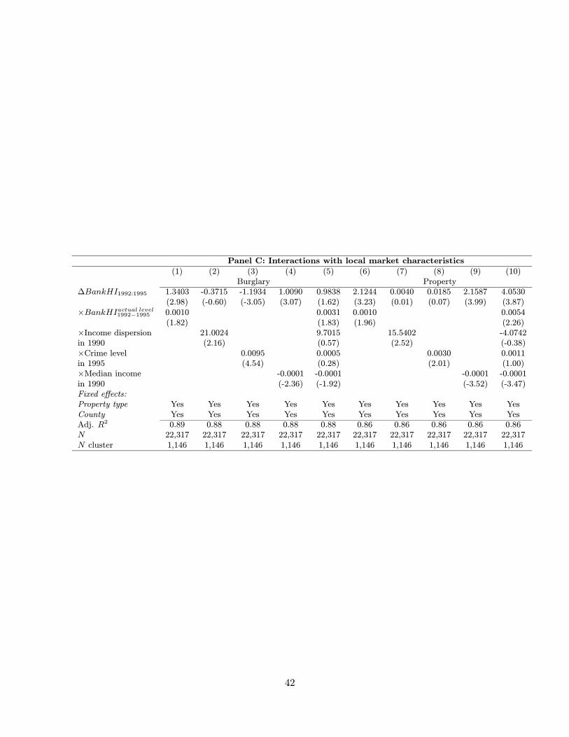
Panel C: Interactions with local market characteristics

(1) (2) (3) (4) (5) (6) (7) (8) (9) (10)Burglary Property

∆BankHI1992:1995 1.3403 -0.3715 -1.1934 1.0090 0.9838 2.1244 0.0040 0.0185 2.1587 4.0530(2.98) (-0.60) (-3.05) (3.07) (1.62) (3.23) (0.01) (0.07) (3.99) (3.87)

×BankHIactual level1992−1995 0.0010 0.0031 0.0010 0.0054(1.82) (1.83) (1.96) (2.26)

×Income dispersion 21.0024 9.7015 15.5402 -4.0742in 1990 (2.16) (0.57) (2.52) (-0.38)×Crime level 0.0095 0.0005 0.0030 0.0011in 1995 (4.54) (0.28) (2.01) (1.00)×Median income -0.0001 -0.0001 -0.0001 -0.0001in 1990 (-2.36) (-1.92) (-3.52) (-3.47)Fixed effects:Property type Yes Yes Yes Yes Yes Yes Yes Yes Yes YesCounty Yes Yes Yes Yes Yes Yes Yes Yes Yes YesAdj. R2 0.89 0.88 0.88 0.88 0.88 0.86 0.86 0.86 0.86 0.86N 22,317 22,317 22,317 22,317 22,317 22,317 22,317 22,317 22,317 22,317N cluster 1,146 1,146 1,146 1,146 1,146 1,146 1,146 1,146 1,146 1,146

42

Table V:Does (Whatever Drives) Future Crime Spur Current Mergers?

The first two columns of Panel A report results from regressions of the percentage change in the current crime risk from 1990 to1995 on the contemporaneous bank merger variable for local bank concentration. Columns 3 and 4 report regression results of theactual future change in banking concentration from 1996 to 1999 on recent trends in crime risk, median income, and home value forthe census tract. The first two (last two) columns of Panel B report regression results of the change in banking concentration due tomergers from 1996 to 1999 (probability of a merger) on recent trends in crime risk, median income, and home value. The first two(last two) columns of Panel C report results from regressions of future changes in crime from 1995 to 2000 on the predicted changein bank concentration due to mergers involving a failing bank (changes in the number of non-lending financial institutions from 1990to 1995). Non-lending financial institutions are obtained from the County Business Patterns of the Bureau of Economic Analysisand are defined as the number of establishments with NAICS codes of 523, 524, and 525. All regressions include a constant, andthe control variables from Table IV. Coefficient estimates and their associated t-statistics (in parentheses) are reported with robuststandard errors that assume group-wise clustering at the zip code level for all regressions except those for non-lending financialinstitutions, which assume group-wise clustering at the county level.

Panel A: Are crime and merger-induced bank Does crime or economic activityconsolidation contemporaneously related? predict future bank consolidation?

Dependent variable = %∆ Crime1990:1995 ∆BankHIactual1996:1999

(1) (2) (3) (4)Burglary Property Burglary Property

∆BankHI1992:1995 0.0398 -0.0432(0.20) (-0.37)

%∆ Crime1990:1995 -0.0061 -0.0346(-0.35) (-1.54)

Income growth 0.0005 0.0003(0.47) (0.24)

Home value growth -0.0006 -0.0006(-1.65) (-1.92)

County fixed effects Yes Yes Yes YesN 22,317 22,317 22,317 22,317N cluster 1,146 1,146 1,146 1,146

Panel B: Does crime or economic activity predict Does crime or economic activitybank consolidation due to mergers? predict merger activity?

Dependent variable = ∆BankHI1996:1999 Probability of a merger(1) (2) (3) (4)

Burglary Property Burglary Property

%∆ Crime1990:1995 -0.0008 -0.0005 -0.0935 -0.0897(-1.54) (-0.76) (-2.59) (-2.08)

Income growth 0.0001 0.0001 0.0058 0.0064(0.98) (1.09) (0.65) (0.72)

Home value growth 0.0001 0.0001 -0.0027 -0.0025(1.20) (1.24) (-0.74) (-0.70)

County fixed effects Yes Yes Yes YesN 22,317 22,317 22,317 22,317N cluster 1,146 1,146 1,146 1,146

Panel C: Do mergers of failing banks Do changes in #non-lending financialpredict future crime risk? institutions predict crime risk?

Dependent variable = %∆ Crime1995:2000 %∆ Crime1995:2000(1) (2) (3) (4)

Burglary Property Burglary Property

∆BankHIfailing1992:1995 0.2750 -0.3223(0.98) (-1.87)

∆ Non-lending1990:1995 -0.0006 -0.0186(-0.24) (-1.51)

County fixed effects Yes Yes No NoN 22,317 22,317 22,317 22,317N cluster 1,146 1,146 53 53

43

Table VI:Separating the Merger Effect from the Competition Effect

Panel A reports results from regressions of the actual change in bank loan concentration, loan rate, loansize, and future change in crime risk on the predicted change in local banking competitiveness measuredthrough mergers between non-failing banks and bank holding companies with at least $1 billion in assets,∆BankHIyr1:yr2 , and a dummy variable for the presence of a merger. The former variable captures thepredicted competitive effects of mergers and the latter captures the effect of the merger per se, irrespectiveof its competitive effects. Panel B repeats the regressions on the merger dummy variable alone for only thoseproperties residing in an area where mergers have no predicted effect on competition (i.e., where the continuousmeasure ∆BankHIyr1:yr2 = 0). All regressions include a constant and all of the control variables from TablesII and IV, including property type and county fixed effects as well as year and bank fixed effects for the loanterm regressions. Coefficient estimates and their associated t-statistics (in parentheses) are reported withrobust standard errors that assume group-wise clustering at the zip code level.

Panel A: All property transactions

Changes in future crime(1) (2) (3) (4)Loan Loan %∆Crime1995:2000

Dependent variable = rate size Burglary Property

∆BankHI1992:1995 0.3825 0.3991(2.29) (2.49)

∆BankHI1992:saleyear 22.2663 -1.3444(2.76) (-1.76)

Merger dummy -0.0588 0.0168 -0.0003 0.0013(-1.12) (2.82) (-0.27) (1.38)

Fixed effects:Year Yes Yes No NoProperty type Yes Yes Yes YesCounty Yes Yes Yes YesBank Yes Yes No NoAdj. R2 0.28 0.03 0.87 0.86N 6,267 11,809 22,317 22,317N cluster 915 1,100 1,146 1,146

Panel B: Mergers with no predicted competitive effects, ∆BankHI = 0

Changes in future crime(1) (2) (3) (4)Loan Loan %∆Crime1995:2000

Dependent variable = rate size Burglary Property

Merger dummy 0.0552 0.0278 0.0001 0.0001(0.47) (8.72) (0.09) (0.10)

Fixed effects:Year Yes Yes No NoProperty type Yes Yes Yes YesCounty Yes Yes Yes YesBank Yes Yes No NoAdj. R2 0.34 0.03 0.84 0.78N 3,593 5,958 14,544 14,544N cluster 580 688 801 801

44

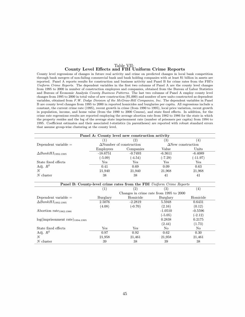
Table VII:County Level Effects and FBI Uniform Crime Reports

County level regressions of changes in future real activity and crime on predicted changes in local bank competitionthrough bank mergers of non-failing commercial bank and bank holding companies with at least $1 billion in assets arereported. Panel A reports results for construction and business activity and Panel B for crime rates from the FBI’sUniform Crime Reports. The dependent variables in the first two columns of Panel A are the county level changesfrom 1995 to 2000 in number of construction employees and companies, obtained from the Bureau of Labor Statisticsand Bureau of Economic Analysis County Business Patterns. The last two columns of Panel A employ county levelchanges from 1995 to 2000 in total value of new construction ($1,000) and number of new units constructed as dependentvariables, obtained from F.W. Dodge Division of the McGraw-Hill Companies, Inc. The dependent variables in PanelB are county level changes from 1995 to 2000 in reported homicides and burglaries per capita. All regressions include aconstant, the current crime rate (1995), recent growth in crime (from 1990 to 1995), local price variation, recent growthin population, income, and home value (from the 1990 to 2000 Census), and state fixed effects. In addition, for thecrime rate regressions results are reported employing the average abortion rate from 1982 to 1986 for the state in whichthe property resides and the log of the average state imprisonment rate (number of prisoners per capita) from 1994 to1995. Coefficient estimates and their associated t-statistics (in parentheses) are reported with robust standard errorsthat assume group-wise clustering at the county level.

Panel A: County level new construction activity

(1) (2) (3) (4)Dependent variable = ∆Number of construction ∆New construction

Employees Companies Value Units∆BankHI1992:1995 -18.6751 -0.7493 -6.3611 -6.4089

(-5.09) (-4.54) (-7.29) (-11.97)State fixed effects Yes Yes Yes YesAdj. R2 0.41 0.69 0.09 0.63N 21,940 21,940 21,968 21,968N cluster 38 38 41 41

Panel B: County-level crime rates from the FBI Uniform Crime Reports

(1) (2) (3) (4)Changes in crime rate from 1995 to 2000

Dependent variable = Burglary Homicide Burglary Homicide∆BankHI1992:1995 2.5076 -2.2819 5.5948 0.6431

(4.08) (-0.70) (2.16) (0.12)Abortion rate1982:1986 -1.0510 -0.5596

(-5.05) (-2.12)log(imprisonment rate)1994:1995 0.2838 0.2175

(2.44) (1.73)State fixed effects Yes Yes No NoAdj. R2 0.97 0.92 0.62 0.30N 21,958 21,461 21,958 21,461N cluster 39 38 39 38

45

Table VIII:The Impact of State-Level Bank Branching Regulation onBank Concentration, Loan Activity, Prices, and Crime

Panel A employs commercial property transaction level data from COMPS from 1992 to 1999. Regressions of the level oflocal bank concentration, loan rate, loan size, and capitalization rate of properties on the number of years since the state firstallowed unrestricted branching (takes on the value zero if the state had yet to institute unrestricted branching at the time ofthe property sale) are reported. Regressions include a constant, current crime risk (1995), recent growth in crime (from 1990to 1995), recent growth in population, income, and home value, and property type fixed effects. Loan rate regressions alsoinclude the loan attributes from Table II. Coefficient estimates and their associated t-statistics (in parentheses) are reportedwith robust standard errors that assume group-wise clustering at the state and year level. Panel B employs state-level data oncrime rates (reported homicides and burglaries per 1,000 people) from the FBI’s Uniform Crime Reports from 1978 to 2001.The year-to-year percentage changes in crime rates are regressed on a state level bank branching indicator which takes onthe value one if the state had adopted unrestricted branching within the last five years. Regressions also include a constant,the one year lagged change in state population, employment, social services (the number of social service employees percapita), income, and imprisonment rate (number of prisoners per capita), as well as the 16 year lagged change in the stateabortion rate (×1, 000), which is the change in the number of abortions (16 years ago) per 1,000 live births. Cross-sectionalregressions across all 50 states plus the District of Columbia are run each year from 1978 to 2001 (1987 to 2001 when includingabortion rates) in the style of Fama and MacBeth (1973), where the time-series average of the yearly cross-sectional regressioncoefficient estimates are reported along with their time-series t-statistics (in parentheses).

Panel A: Transaction level loan activity and prices from COMPS

(1) (2) (3) (4)Dependent variable = Actual Loan Loan Cap rate

BankHI rate size (E/P)

Years of unrestricted branching -0.0006 -0.0152 0.0015 -0.0230(-3.19) (-2.02) (4.25) (-3.37)

Price variation -0.0074 0.0410 -0.0147 0.6660(-2.24) (0.36) (-1.46) (5.97)

Population growth 0.0002 0.0051 -0.0003 -0.0059(1.78) (0.46) (-0.35) (-0.69)

Income growth 0.0012 0.1401 -0.0001 -0.0499(2.72) (1.34) (-0.66) (-0.40)

Home value growth 0.0001 -0.0003 -0.0001(2.20) (-0.39) (-2.11)

N 22,317 6,267 16,131 10,070N cluster 96 96 96 96

Panel B: State-level changes in crime across all 50 states from the FBI

Fama-MacBeth cross-sectional regressions(1) (2) (3) (4)

Dependent variable = %∆Crimet %∆Homicidet %∆Homicidet %∆Burglaryt %∆Burglarytper 1,000 people (1978—2001) (1987—2001) (1978—2001) (1987—2001)

Post unrestricted branching indicator -0.0094 -0.0143 -0.0150 -0.0100(-0.87) (-1.39) (-3.48) (-3.40)

∆Populationt−1 -0.0001 0.0001 -0.0001 -0.0001(-0.53) (0.49) (-0.48) (-1.08)

∆Employmentt−1 5.5718 4.8934 0.7494 0.5595(5.03) (5.39) (2.71) (2.12)

∆Social servicest−1 -0.0070 -0.0056 -0.0029 -0.0042(-4.21) (-5.72) (-6.25) (-9.36)

∆Incomet−1 -23.981 -14.509 -3.4942 2.8806(-3.31) (-2.48) (-1.70) (2.32)

∆Imprisonment ratet−1 -0.0261 -0.0106 0.0129 0.0088(-1.29) (-1.09) (2.68) (2.35)

∆Abortion ratet−16 -0.3173 -0.1007(-5.75) (-6.08)

N (# years) 24 15 24 15

46

Summary statisics

Mean Std. Dev. 75th% 90th% Max∆BankHI1992:1995 0.0010 0.0028 0.0011 0.0040 0.0417those > 0 0.0031 0.0040 0.0040 0.0043

∆BankHI1992:saleyear 0.0025 0.0050 0.0030 0.0060 0.0721those > 0 0.0051 0.0061 0.0052 0.0123

∆BankHI1992:1999 0.0048 0.0068 0.0055 0.0167 0.0721those > 0 0.0073 0.0072 0.0088 0.0179

0 0.01 0.02 0.03 0.04 0.05 0.06 0.070

0.2

0.4

0.6

0.8

1

1.2

1.4

1.6

1.8

2x 10

4 Distribution for Entire Sample

Predicted Change in Bank Herfindahl Concentration Index from Mergers

Freque

ncy

1992:19951992:Saleyear1992:1999

0.01 0.02 0.03 0.04 0.05 0.06 0.070

200

400

600

800

1000

1200

1400

1600

1800Distribution Excluding Zeros

Predicted Change in Bank Herfindahl Concentration Index from Mergers

Freque

ncy

1992:19951992:Saleyear1992:1999

Figure 1. Distribution of Predicted Change in Bank Concentration from Mergers of Non-failing Commercial

Bank and Bank Holding Companies with Assets Greater than $1 Billion. The predicted change in banking compet-

itiveness from year yr1 to yr2 caused by mergers, ∆BankHIyr1:yr2 , is defined as the sum of the individual year increases in

the Herfindahl concentration index,∆BankHIyr1:yr2,j =yr2yr=yr1

BankHImergej,yr −BankHIactualj,yr , where BankHIactualj,yr

is the actual Herfindahl concentration index of commercial real estate bank loans within 15 miles of property j (excluding j

itself) and BankHImergej,yr is the hypothetical concentration index assuming all non-failing commercial bank mergers took place

at the beginning of each year. The range of years used in calculating ∆BankHIyr1:yr2,j are 1992 to 1995, 1992 to saleyear,

where saleyear is the year in which the property transacted, and 1992 to 1999. The distribution and summary statistics for

the entire sample and only those where the predicted change in concentration is positive are reported.

47