BANK CAPITAL AND LENDING BEHAVIOR: EMPIRICAL EVIDENCE FOR ITALY

by Leonardo Gambacorta* and Paolo Emilio Mistrulli*

This version: February 14, 2003

Abstract

This paper investigates the existence of cross-sectional differences in the response of lending to monetary policy and GDP shocks due to a different degree of bank capitalization. The effects on lending of shocks to bank capital, that are caused by a specific (higher than 8 per cent) solvency ratio for highly risky banks, are also analyzed. The paper adds to the existing literature in three ways. First, it considers a measure of capitalization (the excess capital) that is better able to control for the riskiness of bank’s portfolio than the well-known capital-to-asset ratio. Second, it disentangles the effects of the “bank lending channel” from those of the “bank capital channel” in the case of a monetary shock; it also provides an explanation for asymmetric effects of GDP shocks on lending based on the link between bank capital and risk-aversion. Third, it uses a unique dataset of quarterly data for Italian banks over the period 1992-2001; the full coverage of banks and the long sample period helps to overcome some distributional bias detected for other public available dataset. The results indicate that well-capitalized banks can better shield their lending from monetary policy shocks as they have, consistently with the “bank lending channel” hypothesis, an easier access to non-deposit fund raising. A “bank capital channel” is also detected, with higher effects for cooperative banks that suffer a higher maturity mismatching. Capitalization also influences the way banks react to GDP shocks. Again, the credit supply of well-capitalized banks is less pro-cyclical. The introduction of a specific solvency ratio for highly risky banks determines an overall reduction in lending.

JEL classification: E44, E51, E52

Keywords: Basle standards, monetary transmission mechanisms, bank lending, bank capital.

Index

1. Introduction.......................................................................................................................... 2 2. Bank capital and the business cycle..................................................................................... 5 3. Some stylized facts on bank capital................................................................................... 10 4. The econometric model and the data ................................................................................. 14 5. The results.......................................................................................................................... 18

5.1 Robustness checks ...................................................................................................... 21 6. Conclusions........................................................................................................................ 22 Appendix 1 – A simple theoretical model.............................................................................. 25 Appendix 2 - Description of the database .............................................................................. 33 References .............................................................................................................................. 35

* Banca d’Italia, Research Department.

1. Introduction1

The role of bank capital in the monetary transmission mechanism has been largely

neglected by economic theory. The traditional interpretation of the “bank lending channel”

focuses on the effects of reserve requirements on demand deposits, while no attention is paid

to bank’s equity; bank capital is traditionally interpreted as an “irrelevant” balance sheet

item (Friedman, 1991; Van den Heuvel, 2003). Moreover, in contrast with the wide literature

that analyzes the link between risk aversion and wealth, there is scarce evidence on the

relationship between a bank’s risk attitude and her level of capitalization. This lack of

attention contrasts with the importance given, both at an empirical and theoretical level, to

the macroeconomic consequences of the Basle Capital Accord that designed risk-based

capital requirements for banks.2

The main aim of this paper is to study how bank capital may influence the response of

lending to monetary policy and GDP shocks. There are two ways in which bank capital may

affect the impact of monetary shocks: through the traditional “bank lending channel” and

through a more “direct” mechanism defined “bank capital channel”. Both channels rest on

the failure of the Modigliani-Miller theorem of the financial structure irrelevance but, as we

will discuss, for different reasons.

Bank’s capitalization influences the “bank lending channel” due to imperfections in the

market for debt. In particular, bank capital influences the capacity to raise uninsured form of

debt and therefore bank’s ability to contain the effect on lending of a deposit drop. The

mechanism is the following. After a monetary tightening, reservable deposits drop and banks

raise non-reservable debt in order to protect their loan portfolios. As these non-reservable

funding are typically uninsured (i.e. bonds or CDs), banks encounter an adverse selection

problem (Stein, 1998); low capitalized banks, perceived more risky by the market, have

1 The authors are grateful to Giorgio Gobbi, Simonetta Iannotti, Francesco Lippi, Silvia Magri, Alberto

Franco Pozzolo, Skander Van den Heuvel and an anonymous referee for useful comments. The model owes a lot to discussions with Michael Ehrmann, Jorge Martinez-Pagès, Patrick Sevestre and Andreas Worms. The usual disclaimer applies. The opinions expressed in this paper are those of the authors only and in no way involve the responsibility of the Bank of Italy. Email gambacorta.leonardo@insedia.interbusiness.it; mistrulli.paoloemilio@insedia.interbusiness.it.

2 See Basle Commitee on Banking Supervision (1999) for a reference on the subject.

3

more difficulties to issue bonds and have therefore less capacity to shield their credit

relationships (Kishan and Opiela, 2000).

The “bank capital channel” is based on three hypotheses: 1) an imperfect market for

bank equity (Myers and Majluf, 1984; Stein, 1998; Calomiris and Hubbard, 1995; Cornett

and Tehranian, 1994); 2) a maturity mismatching between assets and liabilities that exposes

banks to interest rate risk; 3) a “direct” influence of regulatory capital requirements on the

supply of credit. The “bank capital channel” works in the following way. After an increase

of market interest rates, a lower fraction of loans can be renegotiated with respect to deposits

(loans are mainly long term, while deposits are typically short term): banks suffer therefore a

cost due to the maturity transformation performed that reduces profits and then capital. If

equity is sufficiently low (and it is too costly to issue new shares), banks reduce lending

because prudential regulation establishes that capital has to be at least a minimum percentage

of loans (Thakor, 1996; Bolton and Freixas, 2001; Van den Heuvel, 2001a).

Bank capitalization may also influence the reaction of credit supply to output shocks.

This effect depends upon the link between bank capital and risk-aversion. A part of the

literature argue that well-capitalized banks are less risk-averse. In the presence of a solvency

regulation, banks maintain a higher level of capital just because their lending portfolios are

riskier (e.g., Kim and Santomero, 1988; Rochet, 1992; Hellman, Murdock and Stiglitz,

2000). In this case we should observe that well-capitalized banks react more to business

cycle fluctuations because they have selected ex-ante a lending portfolio with higher return

and risk. On the contrary, other models stress that well-capitalized banks are more risk-

averse because the implicit subsidy that derives from deposit insurance is a decreasing

function of capital (e.g., Flannery, 1989; Gennotte and Pyle, 1991) or because they want to

limit the probability not to meet capital requirements (Dewatripont and Tirole, 1994). In this

case, since the quality of the loan portfolio of well-capitalized banks is comparatively higher

they should reduce their lending supply by less in bad states of the nature.

The empirical investigations concerning the effect of bank capital on lending mostly

refer to the US banking system (e.g., Hancock, Laing and Wilcox, 1995, Furfine, 2000,

Kishan and Opiela, 2000; Van den Heuvel, 2001b). All these works underline the relative

importance of bank capital in influencing lending behavior. The literature on European

countries is instead far from conclusive; Altunbas et al. (2002) and Ehrmann et al. (2003)

4

find that lending of undercapitalized banks suffers more from a monetary tightening, but

their results are not significant at conventional values for the main European countries.

This paper presents three novelties with respect to the existing literature. The first one

is the definition of capitalization; we define banks’ capitalization as the amount of capital

that banks hold in excess of the minimum required to meet prudential regulation standards.

This definition allows us to overcome some problems of the capital-to-asset ratio generally

used in the existing literature. Since minimum capital requirements take into account the

quality of banks’ balance sheet activities, the excess capital represents a cushion that controls

for the level of banks’ risk and indicates a lower probability of a bank to go into default.

Moreover, excess capital is a direct measure of banks capacity to expand credit because it

takes into consideration prudential regulation constraints. The second novelty lies in the

tentative to analyze the effects of capitalization on banks response to various economic

shocks. In the case of monetary shocks we separate the effects of the “bank lending channel”

from those of the “bank capital channel”. We provide a tentative explanation of the effect of

GDP shocks on lending based on the link between bank capital and risk-aversion.

Exogenous capital shocks that refer to specific solvency ratio that supervisors set for very

risky banks are also analyzed. The third novelty is the use of a unique dataset of quarterly

data for Italian banks over the period 1992-2001; the full coverage of banks and the long

sample period should overcome some distributional bias detected for other public available

dataset. To tackle problems in the use of dynamic panels, all the models have been estimated

using the GMM estimator suggested by Arellano and Bond (1991).

The results indicate that well-capitalized banks can better shield their lending from

monetary policy shocks as they have, consistently with the “bank lending channel”

hypothesis, an easier access to non-deposit fund raising. In this respect, banks’ capitalization

effect is larger for non-cooperative banks, which are more dependent on non-deposit forms

of external funds. Capitalization also influences the way banks react to GDP shocks. Again,

the credit supply of well-capitalized banks is less pro-cyclical. This result indicates that well-

capitalized banks are more risk-averse and, as their borrowers are less risky, suffer less from

economic downturns via loan losses. Moreover, well-capitalized banks can better absorb

temporarily financial difficulties on the part of their borrowers and preserve long term

lending relationships. Exogenous capital shocks, due to the introduction of a specific (higher

5

than 8 per cent) solvency ratio for highly risky banks, determine an overall reduction of 20

per cent in lending after two years. This result is consistent with the hypothesis that it costs

less to adjust lending than capital.

The remainder of the paper is organized as follows. The next section reviews the

literature and explains the main link between capital requirements and banks’ loan supply.

Section 3 indicates some stylized facts concerning bank capital in Italy. In Section 4 we

describe the econometric model and the data. Section 5 presents our empirical results and the

robustness checks. The last section summarizes the main conclusions.

2. Bank capital and the business cycle

There are several theories that explain how bank capital could influence the

propagation of economic shocks. All these theories suggest the existence of market

imperfections that modify the standard results of the Modigliani and Miller theorem. Broadly

speaking, if capital markets were perfect a bank would always be able to raise funds (debt or

equity) in order to finance lending opportunities and her level of capital would have no role.

The aim of this Section is to discuss how bank capital may influence the reaction of

bank lending to two kinds of economic disturbances: monetary policy and GDP shocks.

The first kind of shock occurs when a monetary tightening (easening) determines a

reduction (increase) of reservable deposits and an increase (reduction) of market interest

rates. In this case, there are two ways in which bank capital may influence the impact of

monetary policy changes on lending: through the traditional “bank lending channel” and

through a more “direct” mechanism defined as “bank capital channel”.

Both mechanism are based on adverse selection problems that affect banks fund-

raising: the “bank lending channel” relies on imperfections in the market for bank debt

(Bernanke and Blinder, 1988; Stein, 1998; Kishan and Opiela, 2000), while the “bank capital

channel” concentrates on an imperfect market for banks’ equity (Thakor, 1996; Bolton and

Freixas, 2001; Van den Heuvel, 2001a).

According to the “bank lending channel” thesis, a monetary tightening has effect on

bank lending because the drop in reservable deposits cannot be completely offset by issuing

6

other forms of funding (or liquidating some assets). Therefore a necessary condition for the

“bank lending channel” to be operative is that the market for non-reservable bank liabilities

is not frictionless. On the contrary, if banks had the possibility to raise, without limit, CDs or

bonds, which are not subject to reserve requirements, the “bank lending channel” would be

ineffective. This is indeed the point of the Romer and Romer critique (1990).

On the contrary, Kashyap and Stein (1995, 2000) and Stein (1998) claim that the

market for bank debt is imperfect. Since non-reservable liabilities are not insured and there is

an asymmetric information problem about the value of banks’ assets, a “lemon’s premium”

is paid to investors. In this case, bank capital has an important role because it affects banks’

external ratings and provides the investors with a signal about their creditworthiness. This

hypothesis implies that banks are subject to “market discipline”. Therefore the cost of non-

reservable funding (i.e. bonds or CDs) would be higher for low-capitalized banks because

they have less equity to absorb future losses and then are perceived more risky by the

market.3 Low-capitalized banks are therefore more exposed to asymmetric information

problems and have less capacity to shield their credit relationships (Kishan and Opiela,

2000).4

It is important to note that this effect of bank capital on the “bank lending channel”

cannot be captured by the capital-to-asset ratio. This measure, generally used by the existing

literature to analyze the distributional effects of bank capitalization on lending, does not take

into account the riskiness of a bank portfolio. A relevant measure is instead the excess

capital that is the amount of capital that banks hold in excess of the minimum required to

meet prudential regulation standards. Since minimum capital requirements are determined by

the quality of bank’s balance sheet activities (for more details see Section 3), the excess

capital represents a risk-adjusted measure of bank capitalization that gives more indications

on the probability of a bank default. Moreover, the excess capital is a relevant measure of the

3 Empirical evidence has found that lower capital levels are associated with higher prices for uninsured

liabilities. See, for example, Ellis and Flannery (1992) and Flannery and Sorescu (1996). 4 The total effect also depends on the amount of bank liquidity. Other things equal, banks with a high buffer

of liquid assets should cut back their lending less in response to a monetary tightening. The intuition of this result is that banks with a large amount of very liquid assets have the option of selling them to shield loan portfolio (Kashyap and Stein, 2000; Ehrmann et al. 2003).

7

availability of the bank to expand credit because it directly controls for prudential regulation

constraints.

The “bank capital channel” is based on three hypotheses. First, there is an imperfect

market for bank equity: banks cannot easily issue new equity for the presence of agency

costs and tax disadvantages (Myers and Majluf, 1984; Stein, 1998; Calomiris and Hubbard,

1995; Cornett and Tehranian, 1994). Second, banks are subject to interest rate risk because

their assets have typically a higher maturity with respect to liabilities (maturity

transformation). Third, regulatory capital requirements limit the supply of credit (Thakor,

1996; Bolton and Freixas, 2001; Van den Heuvel, 2001a).

The mechanism is the following. After an increase of market interest rates, a lower

fraction of loans can be renegotiated with respect to deposits (loans are mainly long term,

while deposits are typically short term): banks suffer therefore a cost due to the maturity

mismatching that reduces profits and then capital. If equity is sufficiently low and it is too

costly to issue new shares, banks reduce lending, otherwise they fail to meet regulatory

capital requirements.

The “bank capital channel” can also be at work even if capital requirement is not

currently binding. Van den Heuvel (2001) shows that low-capitalized banks may optimally

forgo lending opportunities now in order to lower the risk of capital inadequacy in the future.

This is interesting because in reality, as shown in Section 3, most banks are not constrained

at any given time. It is also worth noting that, according to the “bank capital channel”, a

negative effect of a monetary tightening on bank lending could be generated also if banks

face a perfect market for non-reservable liabilities.

Bank capitalization may also influence the way lending supply reacts to output shocks.

Bank capitalization, that is bank wealth, is linked to risk taking behavior and then to banks’

portfolio choices; this means that lending of banks with different degrees of capitalization

(or risk aversion) may react differently to economic downturns. While a wide stream of

literature on financial intermediation has analyzed the relation between bank capitalization

8

and risk taking behavior,5 the nature of this link is still quite controversial. A first class of

models (Kim and Santomero, 1988; Rochet, 1992; Hellman, Murdock and Stiglitz, 2000)

argue that well-capitalized banks are less risk averse. In the presence of a solvency

regulation, well-capitalized banks detain a higher level of capital just because their lending

portfolio is riskier. In this case we should observe that well-capitalized banks react more to

business cycle fluctuations because they have selected ex-ante a lending portfolio with

higher return and risk.

In Kim and Santomero (1988), the introduction of a solvency regulation entails an

inefficient asset allocation by banks. The total volume of their risky portfolio will decrease

(as a direct effect of the solvency regulation), but its composition will be distorted in the

direction of more risky assets (recomposition effect). In this model, the probability of failure

increases after capital requirements are introduced because the direct effect is dominated by

the recomposition of the risky portfolio. On the same line, Hellman, Murdock and Stiglitz

(2000) argue that higher capital requirements are the cause of excessive risk-taking by banks.

Since capital regulation increase banks’ cost of funding (equity is more costly than debt) and

lower the value of the bank, the management of the bank reacts by increasing the level of

credit portfolio risk.6

The main implications of this class of models are three. First, well-capitalized banks

are less risk averse because regulation creates an incentive in doing so. Second, risk-based

capital standards would become efficient only if the weights that reflect the relative riskiness

5 The relation between wealth and attitude towards risk is central to many fields of economics. As far as

credit markets are concerned, this relation has been largely employed in analyzing the role of collateral in mitigating asymmetric information problems between banks and borrowers (see Coco, 2000 for a recent survey on this subject).

6 A different explanation is given by Besanko and Kanatas (1996). They depart from Kim and Santomero (1988) and Hellman, Murdock and Stiglitz (2000) by allowing for outside equity (owned by shareholders who are not in control of the firm) and by stressing the role of managerial incentive schemes in a moral hazard framework. Modeling at the same time asset-substitution (among assets with different risk profiles) and effort aversion moral hazard, they show that while a higher capital requirement reduces asset-substitution problems, it lowers the incentive to exert the optimal amount of effort. This result rests on what they call a “dilution effect”: if bank insiders are wealth-constrained or risk-averse, more stringent capital standards dilute insiders’ ownership share, and thus their marginal benefit of effort. The main conclusion of the model is that, if the effort aversion effect is larger than the asset-substitution effect, higher capital standards induce banks to take on average more risk. Gorton and Rosen (1996) argue that excessive risk taking among well-capitalized banks could also reflect exogenous conditions such as managerial incompetence or a lack of lending opportunities.

9

of assets in the solvency ratio were market-based (Kim and Santomero, 1988).7 In this case

distortion in the banks’ asset allocation disappears and capital requirements reflect the

effective risk taking of the bank.8 Third, these models are not able to explain why banks

typically detain excess capital with respect to the minimum requirements imposed by the

supervisory authority (for example, see van den Heuvel (2003) for the US). As we will see

this is a crucial point in studying heterogeneity in the behavior of banks due to capitalization.

A different result is reached by other models based on a portfolio approach (Flannery,

1989; Gennotte and Pyle, 1991) for which well-capitalized banks are more risk-averse. They

support this result studying the relation between deposit insurance schemes and risk-taking

attitude of banks. If the insurance premium undervalues banks’ risk, the implicit subsidy

from deposit insurance is a decreasing function of capital. That is, highly capitalized banks

are more risk-averse. This means that, since the quality of the loan portfolio of well-

capitalized banks is comparatively higher, they suffer fewer losses in the case of an

economic downturn; the low amount of write-offs allows well-capitalized banks to reduce

their lending supply by less in bad states of the nature. In this class of models the presence of

capital requirements attenuates the distortions caused by deposits guarantees: banks cannot

limit the amount of equity to obtain the maximum implicit subsidy from deposit insurance.

An implication of these models is that if a bank has excess capital with respect to the

minimum requirements she is more risk-averse because she evaluates her risk more

cautiously than the supervisory authority.

The hypothesis that that well-capitalized banks are more risk-averse can be also

supported interpreting excess capital as a cushion against contingencies. When a solvency

regulation is introduced, banks have to face the possibility that they could fail to meet capital

requirements and that, if this really happens, they could loose part of their control in favor of

7 Thakor (1996) proves that a more stringent risk-based standard may reduce banks’ willingness to screen

risky borrowers. In this sense, market pricing of uninsured liabilities (the so-called “market discipline”) could contribute to avoid excessive risk-taking by undercapitalized banks. More cautious conclusions in evaluating the potential effects of subordinated debt requirement are developed in Calem and Rob (1999). Sheldon (1996) provides weak evidence that the implementation of the Basle Accord had a risk-increasing impact on bank portfolio.

8 Analyzing a model with limited liability (capital can not be negative as in Kim and Santomero, 1988) Rochet (1992) suggests introducing an additional regulation, namely a minimum level of capital, independent of the size of the bank assets.

10

supervisors (Dewatripont and Tirole, 1994; Repullo, 2000; van den Heuvel, 2001a).

Therefore, banks choose a certain excess capital at time t taking into account the possibility

that in the future they could not be able to meet regulatory standards. The amount of capital

banks hold in excess to capital requirement depends on their (global) risk aversion that is

independent of the initial level of wealth.9 Differences in (global) risk aversion among banks

may emerge not only for heterogeneity in corporate governance but also, and more

substantially, for institutional reasons. In Italy, as we will discuss in the following section,

the institutional characteristics of credit cooperative banks (CCBs) are very different with

respect to that of limited companies. If we allow for heterogeneity in (global) risk-aversion

among banks the excess capital becomes a crucial measure to capture differences in the risk

profile of banks’ portfolios. The simple capital-to-asset ratio is no longer informative

because it does not capture the constraint due to regulation.

3. Some stylized facts on bank capital

The 1988 Basle Capital Accord and its subsequent amendments require capital to be

above a threshold that is defined as a function of several types of risk. In other words, it is

possible to distinguish between the default risk (credit risk) and the risk related to adverse

fluctuations in asset market prices (market risk). 10 In Italy, the capital requirements for

credit risks have been introduced in 1992, those for market risks in 1995.

As far as credit risk is concerned, capital must be at least equal to 8 per cent of the total

amount of risk-weighted assets (solvency ratio).11 A bank-specific solvency ratio (higher

9 A simple way to say that bank i is globally more averse than bank j is to assume that the objective function of bank i is a concave transformation of bank j objective function.

10 In general the need of capital requirements arises to overcome moral hazard problems inducing banks to detain a “socially optimal” amount of capital. In the event of a crisis, the lower the leverage ratio is, the higher the probability that a bank will fail to pay back its debts. The moral hazard problem is amplified in the presence of a deposit insurance system. For a more detailed explanation of the rationale for capital requirements, see among others, Giammarino, Lewis and Sappington (1993), Dewatripont and Tirole (1994), Vlaar (2000) and Rime (2001).

11 In Italy, regulation establishes a minimum capital requirement as a function of the amount of risk-weighted assets (and certain off-balance sheet activities). Assets are classified into five buckets with different risk weights. Risk weights are zero for cash and government bonds, 20 per cent for bank claims on other banks, 50 per cent for mortgage lending, 100 per cent for other loans on the private sector, 200 per cent for participating in highly risky non financial firms (firms that have recorded losses in the last two years). Till

11

than 8 per cent) can be disposed in case of a poor performance in terms of asset quality,

liquidity and organization. On the contrary, the ratio decreases to 7 per cent for banks that

belong to a banking group that meets an 8 per cent solvency ratio on a consolidated basis.

Capital requirements on market risks are related to open trading positions in securities,

foreign exchange and commodities.12

Banks have to hold an amount of capital that must be at least equal to the sum of credit

and market risk capital requirements.13

One of the objectives of the 1988 Basle Accord was to increase banks’ capitalization

(Basle Committee on Banking Supervision, 1999). We observe that banks’ capitalization

increased during the period that preceded the implementation of the Basle Accord, Italian

(Fig. 1) and it was slightly declining afterwards. It seems therefore that banks have

constituted sufficient capital and reserves endowments before risk-based capital

requirements were implemented. This seems to support the thesis that bank capital is sticky.

Large banks’ capitalization has been constantly lower than the average.14 At the

opposite, credit cooperative banks (CCBs), typically very small, are better capitalized than

September 1996 bad loans weight was also equal to 200 per cent. For any bank j its capital requirement is defined as:

∑=

⋅=⋅5

1iijijjj AkWAk α

where jk is the solvency ratio, jWA the total amount of risk-weighted assets, iα is the risk weight for asset

type i and ijA is the unweighted amount of the i-type asset bank j holds. 12 Market risk capital requirements are computed on the basis of a quite complex algorithm. Regulation

distinguishes between a “specific risk” and a “general risk”. The former refers to losses that can be determined by market price fluctuations, which are specifically related to the issuer economic condition. The latter is related to asset price fluctuations correlated to market developments (systematic risk). The capital requirement depends on issuer characteristics and on the asset maturity. Ceteris paribus, the capital requirement on market risks is lower for banks belonging to a group.

13 Prudential regulation allows banks to meet capital requirements by holding an amount of capital that is defined as the sum of the so-called Tier 1 and Tier 2 capital (regulatory capital). Tier 1 or core capital includes stock issues, reserves and provisions for general banking risks; Tier 2 or supplementary capital consists of general loan loss provisions, ibryd instruments and subordinated debt. Tier 1 capital is required to be equal at least to the 50 per cent of the total. Subordinated debts must not exceed 50 per cent of Tier 1 capital. Recently, banks have been allowed to issue subordinated debts specifically to face market risk requirements (the so-called Tier 3 capital).

14 We have considered large banks those with total assets greater than 10 billions euro at September 2001. To control for mergers we have assumed that consolidation happened at the beginning of the period (see Appendix 2 for further details on merger treatment).

12

other banks. The different capitalization degree among Italian banks could reflect a diverse

capacity to issue capital. As capital is relatively costly, banks minimize their holdings,

subject to different “adjustment costs” constraints. This implies that, ceteris paribus,

capitalization is lower for those banks that incur lower costs in order to adjust their level of

capital. As we have pointed in Section 2, differences in the level of capitalization depend

also on banks’ risk-aversion related to different corporate governance and institutional

settings.

For all groups of banks the excess capital (the amount that banks hold in excess of the

minimum regulatory capital requirement) has been always significantly greater than zero.

This is consistent with the hypothesis that capital is difficult to adjust and banks create a

cushion against contingencies. If we define as itx the ratio between regulatory capital and

capital requirement this should be close to one if banks choose their capital endogenously to

meet the constraint imposed by the supervision authority. In reality we observe that this ratio

is significantly greater than one (Fig. 2). The cushion is lower for large banks with respect to

CCBs. On the basis of the literature discussed in the previous section, this stylized facts is

consistent with the hypothesis that small banks are more risk-averse than large banks.

Figure 3 shows the time evolution of the deviation of excess capital from its long run

equilibrium. For each bank i at time t, the bank deviation is defined as: ix

iitit σ

xxz

−= where,

ix is the bank capitalization average and ixσ is the standard error of itx . We can interpret ix

as a proxy of the long-run equilibrium capitalization, that we assume to be bank specific. We

then calculate, at every time t, the aggregate index as a mean of each bank index.

We have split banks into three different groups: large banks, other banks (CCBs

excluded), and CCBs. The indicator is more stable for large banks, more volatile for CCBs.

This seems consistent with the view that large banks have easier access to capital markets

and therefore can adjust more rapidly their capitalization degree to loan demand fluctuations;

capitalization is less flexible for smaller banks and for CCBs, which are more dependent on

self-financing.

13

Figure 4 shows the maturity transformation performed by banks. As we have discussed

in the previous section the existence of a maturity mismatching between assets and liabilities

is a necessary condition for the “bank capital channel” to be at work. Since loans have

always typically a longer maturity than bank fund-raising, the average maturity of total

assets is higher than that of liabilities. In this case, as predicted by the “bank capital

channel”, the bank suffers a cost when interest rates are raised and obtains a gain vice versa.

The difference between the average maturity of assets and that of liabilities is higher for

CCBs than for other banks. In fact, CCBs balance sheets are characterized by a higher

percentage of long-term loans, while their bonds issues are more limited. For example, at the

end of September 2002, the ratio between medium and long-term loans over total loans was

57 per cent for CCBs and 46 per cent for other banks. On the contrary, the ratio between

bond and total fund raising was, respectively, 27 and 29 per cent. These differences were

even higher at the beginning of our sample period. Therefore, the analysis of the maturity

mismatching between assets and liabilities indicates room for the existence of a “bank

capital channel” in Italy with a potential higher effect for CCBs.

There is no conclusive evidence about the effects of bank capital on lending behavior

of Italian banks. In principle the financial structure of the Italian economy during the nineties

makes more likely that a “bank lending channel” was at work (see Gambacorta, 2001). Most

empirical papers based on VAR analysis confirm the existence of such a channel in Italy

(Buttiglione and Ferri, 1994; Angeloni et al., 1995; Bagliano and Favero, 1995; Fanelli and

Paruolo, 1999; Chiades and Gambacorta, 2003). However there is much less evidence on

cross sectional differences in the effectiveness of the “bank lending channel” in Italy, due to

capitalization (see de Bondt, 1999; Favero et al., 2001; King 2002; that analyze mainly the

effect of banks dimension and liquidity; some evidence of the effect of capitalization on

lending of Italian banks is detected by Altunbas, 2002). So far no evidence has been

provided on the existence of the so-called “bank capital channel”.

Apart from the differences in specification, all these paper use the BankScope dataset

that, as pointed out by Ehrmann et al. (2003), suffers of two weaknesses. First, the data are

collected annually, which might be too infrequent to capture the adjustment of bank

aggregates to monetary policy. Second, the sample of Italian banks available in BankScope

is biased towards large banks. For example, in 1998 only 576 up to 921 Italian banks were

14

included in the BankScope dataset. Moreover the average size of a bank was 3.7 billion euro

against 1.7 for the total population. To tackle these problems our analysis will be based on

the Bank of Italy Supervisory Reports database, using quarterly data for the full population

of Italian banks.

4. The econometric model and the data

The empirical specification, based on Kashyap and Stein (1995), is designed to test

whether banks with a different degree of capitalization react differently to a monetary policy

or a GDP shock. A simple theoretical framework that justifies the choice of the specification

is reported in Appendix 1.15

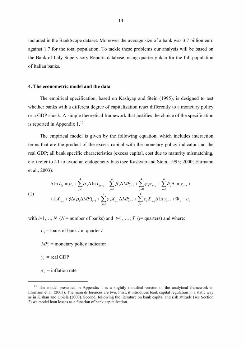
The empirical model is given by the following equation, which includes interaction

terms that are the product of the excess capital with the monetary policy indicator and the

real GDP; all bank specific characteristics (excess capital, cost due to maturity mismatching,

etc.) refer to t-1 to avoid an endogeneity bias (see Kashyap and Stein, 1995; 2000; Ehrmann

et al., 2003):

(1) 1 1 1

4 4 4 4

1 0 0 0

4 4

11 1

ln ln ln

( ) lnit it it

it i j it j j t j j t j j t jj j j j

i t j t j j t j it itj j

L L MP y

X MP X MP X y

µ α β ϕ π δ

λ φ ρ γ τ ε− − −

− − − −= = = =

− − −= =

∆ = + ∆ + ∆ + + ∆ +

+ + ∆ ∆ + ∆ + ∆ + Φ +

∑ ∑ ∑ ∑

∑ ∑

with i=1,…, N (N = number of banks) and t=1, …, T (t= quarters) and where:

itL = loans of bank i in quarter t

MPt = monetary policy indicator

ty = real GDP

π t = inflation rate

15 The model presented in Appendix 1 is a slightly modified version of the analytical framework in

Ehrmann et al. (2003). The main differences are two. First, it introduces bank capital regulation in a static way as in Kishan and Opiela (2000). Second, following the literature on bank capital and risk attitude (see Section 2) we model loan losses as a function of bank capitalization.

15

itX = measure of excess capital

itρ = cost per unit of asset that the bank incurs in case of a one per cent increase in MP

itΦ = control variables.

The model allows for fixed effects across banks, as indicated by the bank-specific

intercept µi. Four lags have been introduced in order to obtain white noise residuals. The

model is specified in growth rates in order to avoid the problem of spurious correlations

among variables that are likely to be non-stationary.

The sample used goes from the third quarter of 1992 to the third quarter of 2001. The

interest rate taken as monetary policy indicator is that on repurchase agreements between the

Bank of Italy and credit institutions in the period 1992-1998, and the interest rates on main

refinancing operation of the ECB for the period 1999-2001.16

CPI inflation and the growth rate of real GDP are used to control for loan demand

effects. The introduction of these two variables allows us to capture cyclical movements and

serves to isolate the monetary policy component of interest rate changes.17

To test for the existence of asymmetric effects due to bank capitalization, the following

measure has been adopted:

//it itit i

it tit t

EC AECX TA N

= −

∑∑

where EC stands for excess capital (regulatory capital minus capital requirements) and A

represents total assets. The excess capital indicator is normalized with respect to the average

across all the banks in the respective sample, in order to obtain a variable that sums to zero

over all observations. This has two implications. First, the sums of the interaction terms

16 As pointed out by Buttiglione, Del Giovane and Gaiotti (1997), in the period under investigation the repo

rate mostly affected the short-term end of the yield curve and, as it represented the cost of banks’ refinancing, it represented the value to which market rates and bank rates eventually tended to converge. It is worth noting that the interest rate on main refinancing operation of the ECB does not present any particular break with the repo rate.

17 For more details on data sources, variable definitions, merger treatment, trimming of the sample and outlier elimination see Appendix 2.

16

1

4

1itj t j

j

X MPγ− −

=

∆∑ and 1

4

1

lnitj t j

j

X yτ− −

=

∆∑ in equation (1) are zero for the average bank

(1it

X−

=0). Second, the coefficients jβ and jδ are directly interpretable, respectively, as the

average monetary policy effect and the average GDP effect.

To test for the existence of a “bank capital channel” we have introduced a variable

( i MPρ ∆ ) that represents the bank-specific interest rate cost due to maturity transformation.

In particular iρ measures the loss (gain) per unit of asset the bank suffers (obtains) when the

monetary policy interest rate is raised (decreased) of one percentage point. We have

computed this variable according to supervisory regulation relative to interest rate risk

exposure that depends on the maturity mismatching among assets and liabilities.18 In other

words, if bank’s assets have a higher maturity with respect to liabilities iρ is positive and

indicates the cost for unit of asset a bank suffers if interest rate are raised by one per cent. To

work out the real cost we have therefore multiplied this measure for the realized change in

interest rates. The term i MPρ ∆ represents the real cost (gain) that a bank suffers (obtains) in

each quarter. As formalized in Appendix 1, this measure influences the level of loans. Since

here the dependent variable is a growth rate we have included this measure in first

differences.

The set of control variables itΦ include a liquidity indicator, given by the sum of cash

and securities to total assets ratio, and a size indicator, given by the log of total assets. The

liquidity indicator has been normalized with respect to the mean over the whole sample

period, while the size indicator has been normalized with respect to the mean on each single

period. This procedure removes trends in size (for more details see Gambacorta, 2001). As

for the other bank specific characteristics also liquidity and size indicators refer to t-1 to

avoid an endogeneity bias.

The fact that supervisors can set solvency ratios greater than 8 per cent for highly risky

banks (see Section 3), allows us to test for the effects of exogenous capital shocks on bank

lending. We analyze the impact of these supervisory actions on lending in the first two years,

18 See Appendix 2 for further details.

17

computing different dummy variables (one for each quarter following the solvency ratio

raise) that equal 1 for banks whose solvency ratio is higher than 8 per cent. This allows us to

capture bank lending adjustment process. A specific dummy variable controls for the effects

of the introduction of market risk capital requirements in the first quarter of 1995.

The sample represents 82 per cent of total bank credit in Italy. Table 1 gives some

basic information on what bank balance sheets look like. Credit Cooperative Banks (CCBs)

are treated separately because they are significantly smaller, more liquid and better

capitalized than other banks. This evidence is consistent with the view that smaller banks

need bigger buffer stocks of securities because of their limited ability to raise external

finance on the financial market. This interpretation is confirmed on the liability side, where

the percentage of bonds is lower among CCBs. The high capitalization of CCBs is, at least in

part, due to the Banking Law prescription that limits significantly the distribution of net

profits.19

Within each category, banks have been split, according to their capitalization.20 Low-

capitalized banks are, independently of their form (CCBs or other banks), larger, less liquid

and they issue more bonds than well-capitalized banks. While these differences are small

among CCBs, they are quite significant among non-CCBs. Among non-cooperative banks,

low-capitalized banks are much larger than well-capitalized ones; a higher share is listed and

belongs to a banking group. Moreover, they issue more subordinated debt to meet the capital

requirement. This evidence is consistent with the view that, ceteris paribus, capitalization is

lower for those banks that bear less adjustment costs from issuing new (regulatory) capital;

large and listed banks can more easily raise funds on the capital market and they can also

rely on a wider set of “quasi-equity” securities that can be issued to meet capital

requirements (e.g. subordinated debts); at the same time, banks belonging to a group can

19 According to art. 37 of the 1993 Banking Law “Banche di credito cooperativo must allocate at least

seventy per cent of net profits for the year to the legal reserve.” 20 A “lowly capitalized” bank has a capital ratio equal to the average capital ratio below the 10th percentile,

a “highly capitalized” bank, that of the banks above the 90th percentile. Since the characteristics of each bank could change over time, percentiles have been worked out on mean values.

18

better diversify the risk of regulatory capital shortage if an internal capital market is active

at the group level.21

5. The results

The results of the study are summarized in Table 2, which presents the long-run

elasticities of bank lending with respect to the variables.22 The models have been estimated

using the GMM estimator suggested by Arellano and Bond (1991) which ensures efficiency

and consistency provided that the models are not subject to serial correlation of order two

and that the instruments used are valid (which is tested for with the Sargan test).23

The existence of asymmetric effects due to bank capital is tested considering three

samples. The first one includes all banks and is our benchmark regression; the other two

consider separately credit cooperative and other banks. These sample splits are intended to

capture differences in the bank capital effect due to the institutional characteristics discussed

in the previous sections.

21 Houston and James (1998) analyze the role of internal capital markets for banks liquidity management.

The same framework could be applied to soften the regulatory capital constraint among banks belonging to the same group.

22 For example, the long-run elasticity of lending with respect to monetary policy for the average bank

(reported on the second row of Table 2) is given by 4 4

0 1/(1 )j j

j jβ α

= =

−∑ ∑ , while that with respect to the interaction

term between excess capital and monetary policy is represented by 4 4

1 1/(1 )j j

j jγ α

= =

−∑ ∑ (see the fifth row of Table

2). Therefore the overall long-run elasticity of the dependent variable with respect to monetary policy for a

well-capitalized bank (seventh row) is worked out through 4 4

0 1/(1 )j j

j jβ α

= =

−∑ ∑ +4 4

1 1/(1 )j j

j jγ α

= =

−∑ ∑ 0.90X > , where

0.90X > is the average excess capital for the banks above the 90th percentile. It is interesting to note that testing the null hypothesis that monetary policy effects are equal in the long-run among banks with different

capitalization corresponds to testing H0: 4

1j

jγ

=∑ =0 using the t-statistic of

4

1j

jγ

=∑ in equation (1). Standard errors

for the long-run effect have been approximated with the “delta method” which expands a function of a random variable with a one-step Taylor expansion (Rao, 1973). In order to increase the degree of freedom we have dropped the contemporaneous and the fourth lags that were statistically not different from zero.

23 In the GMM estimation, instruments are the second and further lags of the quarterly growth rate of loans and of the bank-specific characteristics included in each equation. Inflation, GDP growth rate and the monetary policy indicator are considered as exogenous variables.

19

From the first row of the table it is possible to note that the effect of excess capital on

lending is always significant and positive: well-capitalized banks are less constrained by

capital requirements and have more opportunity to expand their loan portfolio. The effect is

higher for CCBs than for other banks because they encounter higher capital adjustment

costs: CCBs are more dependent on self-financing and cannot easily raise new regulatory

capital.

The response of bank lending to a monetary policy shock has the expected negative

sign. These estimates roughly imply that a 1 per cent increase in the monetary policy

indicator leads to a decline in lending of around 1.2 per cent for the average bank. The effect

is higher for CCBs (-1.8 per cent) than for other banks (-0.2 per cent), that have more access

to markets for non-reservable liabilities. Testing the null hypothesis that monetary policy

effects are equal among banks with a different degree of capitalization is identical to testing

the significance of the long run coefficient of the interaction between excess capital and the

monetary policy indicator (see “Excess capital*MP” in table 2). As predicted by the “bank

lending channel” hypothesis the effects of a monetary tightening are lower for banks with a

higher capitalization, which have easier access to non-deposit financing. Bank capitalization

interaction with monetary policy is very high (in absolute value) for non-CCBs, which are

more dependent on non-deposit forms of external funds. It is worth noting that well-

capitalized non-CCBs are completely insulated from the effect of a monetary tightening (the

effect is statistically not different from zero).

The effects of the so-called “bank capital channel” are reported on the eighth row of

Table 2. The coefficients have the expected negative sign for all banks groups. These

estimates roughly imply that an increase (decrease) of one basis point of the ratio between

the maturity transformation cost and total assets determines a reduction (increase) of 1 per

cent in the growth rate of lending. The reduction (increase) is bigger for CCBs that, as seen

in Section 3, have typically a higher maturity mismatching between assets and liabilities. In

fact, CCBs balance sheets are characterized by a higher percentage of long-term loans, while

their bonds issues are more limited. Another possible explanation for the higher effect of the

“bank capital channel” for CCBs could be their lower use of derivatives for shielding the

maturity transformation gap. With these characteristic CCBs suffer a higher cost when

interest rates are raised and obtains a higher gain vice versa. To sum up the results indicate

20

the existence of a “bank capital channel” that amplifies the effects of monetary policy

changes on bank lending and asymmetric effects of such a channel among banks groups.

The models show a positive correlation between credit and output. A 1 per cent

increase in GDP (which produces a loan demand shift) determines a loan increase of around

0.7 per cent. The effect is lower for CCBs than for other banks. This has two main

explanations. First, for CCBs local economic conditions are more important than national

ones; second, they have closer customer relationships because they shall grant credit

primarily to their members (see “The 1993 Banking Law”, Art. 35).

The interaction term between GDP and excess capital is negative. This means that

credit supply of well-capitalized banks is less dependent on the business cycle. This result is

consistent with Kwan and Eisenbeis (1997) where capital is found to have a significantly

negative effect on credit risk. On theoretical ground our findings are consistent with

Flannery (1989) and Gennotte and Pyle (1991) that argue that highly capitalized banks are

more-risk averse and select ex-ante borrowers with a lower probability to go into default.

Their risk-attitude therefore limits credit supply adjustments in bad states of nature,

preserving credit relationships. The latter explanation needs to be discussed with respect to

the institutional categories of Italian banks. From the sample split it emerges indeed that the

coefficient of 1( )i tMPρ −∆ ∆ is highly significant only for CCBs, while there are no

significant asymmetric effects for the other banks. This is consistent with the stylized fact

discussed in Section 3 that CCBs are more risk-averse than other banks. They detain high

levels of excess capital and are more able to insulate the effect of an economic downturn. As

in Vander Vennet and Van Landshoot (2002) capital provides banks with a structural

protection against credit risk changes. Looking at Table 2 well-capitalized CCBs are able to

completely insulate the effect of GDP on their lending. On the other hand, non-CCBs seem

to be risk-neutral: the effect of a 1 per cent increase in GDP on lending does not differ too

much between well-capitalized (1.3 per cent) and poorly capitalized banks (1.5).

As explained in Section 4, the effects of exogenous capital shocks on bank lending are

captured by dummy variables related to the introduction of a specific (higher than 8 per cent)

solvency ratio. In this case there are not many differences among the three samples. The

introduction of specific solvency ratio determines an overall reduction of around 20 per cent

21

in bank lending after two years. The magnitude of the effect is similar among banks groups.

This result seems consistent with the hypothesis that issuing new equity can be costly for a

bank in the presence of agency cost and tax disadvantages (Myers and Majluf, 1984; Stein,

1998; Calomiris and Hubbard, 1995; Cornett and Tehranian, 1994).

5.1 Robustness checks

We have tested the robustness of these results in several ways. The first test was to

introduce additional interaction terms combining excess capital with inflation, making the

basic equation (1):

(2) 1

1 1 1

4 4 4 4

1 0 0 0

4 4 4

11 1 1

ln ln ln

( ) ln

it

it it it

it i j it j j t j j t j j t jj j j j

i t j t j j t j j t j it itj j j

L L MP y X

MP X MP X y X

µ α β ϕ π δ λ

φ ρ γ τ ψ π ε

−

− − −

− − − −= = = =

− − − −= = =

∆ = + ∆ + ∆ + + ∆ + +

+ ∆ ∆ + ∆ + ∆ + + Φ +

∑ ∑ ∑ ∑

∑ ∑ ∑

The reason for this test is the possible presence of endogeneity between inflation and

capitalization; excess capital may be higher when inflation is high or vice versa. Performing

the test, however, nothing changed, and the double interaction was always not significant

(4

1j

j

ψ=

∑ turned out to be statistically not different from zero).

The second robustness check was to compare equation (1) with the following model:

(3)

1

1 1

4

11

4 4

1 1

ln ln ( )

ln

it

it it

it i j it j t i tj

j t j j t j it itj j

L L X MP

X MP X y

µ α θ λ φ ρ

γ τ ε

−

− −

− −=

− −= =

∆ = + ∆ + + + ∆ ∆ +

+ ∆ + ∆ + Φ +

∑

∑ ∑

where all variables are defined as before, and ϑτ describes a complete set of time dummies.

This model completely eliminates time variation and test whether the three pure time

variables used in the baseline equation (prices, income and the monetary policy indicator)

capture all the relevant time effect. The results are presented in the fourth column of Table 2.

Again, the estimated coefficients on the interaction terms do not vary much between the two

kinds of models, which testifies to the reliability of the cross-sectional evidence obtained.

22

A geographical control dummy was introduced in each model, taking the value of 1 if

the main seat of the bank is in the North of Italy and 0 if elsewhere. In all cases the maturity

transformation variable and the interactions between monetary policy and output shocks with

respect to excess capital remained unchanged.

The last robustness check was to include the interaction between monetary policy and

the liquidity indicator in the baseline regression. The reason for this test was to verify if the

asymmetric effects of monetary policy due to excess capital remained relevant; the

interactions between monetary policy and liquidity, indeed represent a significant factor. We

obtain:

(4)

1

1 1 1

4 4 4 4

1 0 0 0

4 4 4

11 1 1

ln ln ln

( ) ln

it

it it it

it i j it j j t j j t j j t jj j j j

i t j t j j t j j t j it itj j j

L L MP y X

MP X MP X y Liq MP

µ α β ϕ π δ λ

φ ρ γ τ ψ ε

−

− − −

− − − −= = = =

− − − −= = =

∆ = + ∆ + ∆ + + ∆ + +

+ ∆ ∆ + ∆ + ∆ + ∆ + Φ +

∑ ∑ ∑ ∑

∑ ∑ ∑

The results, presented in the fifth column of Table 2, confirm that liquidity is an

important factor enabling banks to attenuate the effect of decrease in deposits on lending but,

at the same time, leave unaltered the distributional effects of excess capital. The result on

liquidity is in line with Gambacorta (2001) and Ehrmann et al. (2003); banks with a higher

liquidity ratio are better able to buffer their lending activity against shocks to the availability

of external finance, by drawing on their stock of liquid assets. In these works, however, bank

capital (defined as the capital-to-asset ratio) does not significantly affect the banks’ reaction

to a monetary policy impulse. This additional test therefore allow us to cast some doubt on

the use of the capital-to-asset ratio to capture distributional effects in a lending regression

because this measure poorly approximate the relevant capital constraint under the Basle

standards.

6. Conclusions

This paper investigates the existence of cross-sectional differences in the response of

lending to monetary policy change and output shocks due to a different degree of

capitalization. It adds to the existing literature in three ways. First, it considers a measure of

capitalization that is better able to capture the relevant capital constraint under the Basle

23

standards than the well-known capital to asset ratio. Defining banks’ capitalization as the

amount of capital that banks hold in excess of the minimum required to meet prudential

regulation standards we are able to measure the effect of capital requirements and to reflect

information on the structure of the loan portfolio or its risk characteristics. Second, it

disentangles the effects of the “bank lending channel” (triggered by deposits reduction) from

those of the “bank capital channel” (due to the maturity transformation); different kinds of

shocks on lending for the Italian banking system are analyzed; not only monetary policy

shocks, but also GDP and capital shocks. In the last case, shocks are genuinely exogenous

because they refer to an increase in minimum capital requirements that supervisors set for

very risky banks. Third, it use a unique dataset of quarterly data for Italian banks over the

period 1992-2001; the full coverage of banks and the long sample period should overcome

some distributional bias detected for other public available dataset.

The main results of the study are the following. Well-capitalized banks can better

shield their lending from monetary policy shocks as they have, consistently with the “bank

lending channel” hypothesis, an easier access to non-deposit fund raising. In this respect,

banks’ capitalization effect is larger for non-cooperative banks, which are more dependent

on non-deposit forms of external funds. A “bank capital channel” is also detected, with

higher effects for cooperative banks whose balance sheets are characterized by a higher

maturity mismatching between assets and liabilities. Capitalization also influences the way

banks react to GDP shocks. Again, the credit supply of well-capitalized banks is less pro-

cyclical. This result has at least two explanations. First, well-capitalized banks are more risk-

averse (as argued by Flannery, 1989 and Gennotte and Pyle, 1991) and, as their borrowers

are less risky, suffer less from economic downturns via loan losses. Second, well-capitalized

banks can better absorb temporarily financial difficulties on the part of their borrowers and

preserve long term lending relationships. Exogenous capital shocks, due to the imposition of

a specific (higher than 8 per cent) solvency ratio for highly risky banks, determine an overall

reduction of 20 per cent in lending after two years. This result is consistent with the

hypothesis that it costs less to adjust lending than capital.

This study shows that capital matters for the response of bank lending to economic

shocks. Notwithstanding, it is difficult to draw what are the implications of this result with

respect to the new directions of the Basle Accord that should be implemented in 2005. The

24

main goal of the amendments is to make the risk weights used to calculate the solvency ratio

more risk-sensitive. In fact, as shown in Section 3 the actual buckets are somewhat too crude

and could lead to regulatory arbitrage. The new weights will be dependent on the ratings of

the borrowers given by rating agencies or internal models developed by banks. This has two

consequences. First, the new Basle Accord will affect banks differently, depending on their

riskness: for riskier (safer) banks the level of capital requirement will be higher (lower),

compared with the present regulation that establish a solvency ratio that is almost constant

among different classes of risk for private customers. As a direct consequence, heterogeneity

in the response of lending to GDP shock due to capitalization could be attenuated. On the

other hand, the new capital regulation, by imposing a higher degree of information

disclosure could make “market discipline” more effective thereby reducing the information

problems on which the “bank lending channel” and the “bank capital channel” rely.

Second, the pro/counter-cyclicality of capital regulation will strongly depend upon the

capacity of external rating agencies and internal models to anticipate economic downturns. If

borrowers are downgraded during recession this should lead to higher capital requirements

that could exacerbate the effect on lending. On the contrary, if ratings are able to anticipate

slowdowns or responds smoothly to economic conditions (they are set “through the cycle”)

the effects of monetary policy and GDP shock on lending should be less pronounced.

Appendix 1 – A simple theoretical model

In order to justify the empirical framework adopted for the econometric analysis, in

this Appendix we develop a simple one-period model highlighting the main channels

through which bank capital can affect loan supply (see Kishan and Opiela, 2000; Ehrmann,

2003). A causal interpretation of the step of the model is given in Figure A1.24

Figure A1

The sequential steps of the model

The balance sheet constraint of the representative bank is given by the following

identity:

(A1.1) XRBDSL +++=+

where L stands for loans, S for securities, D for deposits, B for bonds, R for capital

requirements and X for excess capital. At the end of t-1 bank capital, defined as RXK += ,

24 It is worth stressing that this causal interpretation has the only aim to stress that bank-specific

characteristics are given in t-1 and are predetermined with respect to the maximization in t. On the contrary, the steps in t, whose subscript is for simplicity omitted in the model, are simultaneously determined.

t-1 t

Bank capital K is a fixed endowment, determined by the realization of profit at the end of period t-1 The maturity transformation performed by the bank in t is represented by the composition of her balance- sheet at the end of t-1

The management of the bank determines the risk strategy for credit portfolio in period t

Macroeconomic variables: y, p and imare realized

Loan demand is determined by the private sector

The bank maximizes her profit taking into account prudential supervision constraints and loan demand. She chooses the supply of loan.

Profit is realized and the new endowment of capital is equal to: Kt=Kt-1+π t Banks suffer a cost if they fail to meet capital requirements. A new maturity transformation characterizes the bank’s balance sheet.

26

is a given endowment. This hypothesis indicates that the management of the bank (that for

simplicity is also the her owner to rule out informational asymmetries problems) does not

alter the capitalization of the firm buying or selling shares between t-1 and t; capital remains

therefore fixed until period t when it will be modified by the realization of the profit or the

loss (Kt=Kt-1+πt).25

At the beginning of period t the management of the bank determines the risk strategy

for credit allocation. The allocation of credit portfolio among industries, sectors of activity,

geographical areas, depends upon the risk-aversion of the management that we indicate with

θ∈[-∞,+∞]. This measure could be interpreted as an Arrow-Pratt measure of absolute risk

aversion that is equal to zero if the bank is risk neutral. It is worth noting that the decision

upon the risk strategy profile is taken before the actual supply of credit. The latter will be

chosen to meet loan demand after the realization of economic conditions. Therefore, in

choosing the risk profile the management of the bank takes into account the ex-ante

information about the possible distribution of the macro variables (income, price, interest

rates) and selects a strategy for each possible state of the world.

The choice of the risk profile for lending portfolio (that, as we have shown, depends on

the risk-aversion of the management of the bank) has two important implications. First, it

influences the percentage of non-performing loans (j) that are written-off at time t. Second, it

affects the average rate of return of lending since risky loans are associated with a higher

level of return. This means that the risk premium is negatively related to the bank risk

aversion.

In the spirit of the actual BIS capital adequacy rules, R is given by a fixed amount (k)

of loans.26 We assume that capital requirements are linked only to credit risk (loans) and not

25 This is an extreme case of capital costly adjustment that we assume here to simplify the model. This

hypothesis is widely used in the literature (see, amongst others, Koehn and Santomero, 1980; Kim and Santomero, 1988; Rochet, 1992). Issuing new equity can be costly for a bank. The main reasons are agency cost and tax disadvantages (Myers and Majluf, 1984; Stein, 1998; Calomiris and Hubbard, 1995; Cornett and Tehranian, 1994). A discussion on the exogeneity/endogeneity of the capital goes behind the scope of this study. Here exogeneity has been assumed in order to simplify the algebra given that it does not modify the main findings of the model. In the empirical part of the paper this hypothesis is relaxed using the Arellano and Bond (1991) procedure that allows us to control for endogeneity through instruments variables (see Section 4).

26 More complicated version of the capital constraint would have not changed the main result of the analysis. A possible extension of the simple capital requirement rule could be to consider a different weight on

27

to interest rate risk (investment in securities that for simplicity are considered completely

safe).

(A1.2) kLR =

We assume that banks hold capital in excess of capital requirements. This hypothesis is

consistent with the fact that capital requirement constraints are slack for most banks at any

given time. Banks may hold a buffer as a cushion against contingencies (Wall and Peterson,

1987; Barrios and Blanco, 2001) as they face capital adjustment costs or to convey positive

information on their economic value (Leland and Pile, 1977; Myers and Majluf, 1984).

Another explanation is that banks face a private cost of bankruptcy, which reduces their

expected future income. Van den Heuvel (2001a) argues that even if capital requirement is

not currently binding, a low capitalized bank may optimally forego profitable lending

opportunities now, in order to lower the risk of future capital inadequacy. To capture this

aspects in a simple way we assume that banks pay a lump-sum tax if they can not meet

capital requirements in t.

After the realization of macroeconomic variables, the private sector sets its lending

demand. The bank acts on a loan market characterized by monopolistic competition, which

enables her to set the interest rate along the loan demand schedule.27 The interest rate on loan

(il ) is therefore given by: 28

(A1.3) 0 1 2 3d

l mi c L c i c y c p η= + + + + (c0>0, c1>0, c2>0, c3>0)

non-performing loans (j L): R=k1 (1-j) L+ k2 j L, with 1≥k2≥k1≥0. This should reflect that till 1996 the weight applied to non-performing loans were double with respect to performing loans (k2=0.16>k1=0.08). Another possible extension could be to consider a different weight for loans backed by real guarantee. Indeed, loans to the private sector bear a weight of 0.04 if backed by real guarantees, 0.08 in all other cases (non-performing loans backed by real guarantees included).

27 This hypothesis is generally adopted by the existing literature on bank interest rate behavior. For a survey on modeling the banking firm see Santomero (1984). See also Green (1998) and Lim (2000).

28 For simplicity we assume that all banks face the same loan demand schedule, i. e., the coefficients ci for i=0, 1, 2, 3, are equal among banks. The model could be easily extended to a more general case where each coefficient depends upon some bank-specific characteristics but this goes behind the scope of this study. This simplifying hypothesis allows us to concentrate on the effects of bank specific characteristics on loan supply.

28

that is positively related to loan demand (Ld), the opportunity cost of self-financing, proxied

by the money market interest rate (im), the real GDP (y), the price level (p) and to the risk-

premium (η).29

The risk premium in equation (A1.3) is negatively related to the bank’s risk-aversion

that, as discussed before, influences the risk profile of loan portfolio. Therefore, we have:

(A1.4) 0 1η η η θ= + (η0>0, η1<0)

Loans are risky and, in each period, a percentage j of them is written off from the

balance sheet, therefore reducing bank’s profitability. The percentage of loans which goes

into default (j) depends inversely on the state of the economy, proxied by real GDP, and on

the risk-taking behavior of the bank (θ ).Therefore, per-unit loan losses of the bank are given

by:

(A1.5) 0 1 2( , )j y j y j y jθ θ θ= + + (j0<0, j1<0, j2<0)

Equation (A1.5) states that the quality of bank portfolios reacts differently to changes

in the state of the economy and this in turn depends on the bank’s ex-ante risk attitude. The

cross product indicates that write-offs of more risk-averse banks react less to GDP shocks. If

the bank is risk-neutral (θ =0), j depends only on real GDP.

Following the literature that links risk-aversion and bank capital (see Section 2), we

hypothesize that the parameter θ is linked to the excess capital X at the end of period t-1:30

(A1.6) 1tXθ µ −=

29 As far as the GDP is concerned, there is no clear consensus about how economic activity affects credit

demand. Some empirical works underline a positive relation because better economic conditions would improve the number of project becoming profitable in terms of expected net present value and, therefore, increase credit demand (Kashyap, Stein and Wilcox, 1993). This is also the hypothesis used in Bernanke and Blinder (1988). On the contrary, other works stress the fact that if expected income and profits increase, the private sector has more internal source of financing and this could reduce the proportion of bank debt (Friedman and Kuttner, 1993). On the basis of the evidence provided by Ehrmann et al. (2001) for the four main countries of the euro area and by Calza et al. (2001) for the euro area as a whole, we expect that the first effect dominates and that a higher income determines an increase in credit demand (c2>0).

30 An analysis of the causal direction of influence between capital (wealth) and risk-aversion goes behind the scope of this paper. In the model we suppose that this link is bi-directional. For a discussion on the link between bank capital and risk-aversion see Section 2.

29

It is worth noting that we analyze the link between risk-aversion and excess capital

instead of the level of capital. As discussed in the introduction and in Section 2, the excess

capital is a risk-adjusted measure of bank’s wealth that is independent of prudential

supervision constraints and therefore can be correctly studied with respect to risk-aversion.

On the contrary, the level of capital, largely used in the existing literature, does not give

information on the structure of the loan portfolio or its risk characteristics.

As discussed in Section 2, the effect of the excess capital on banks’ risk attitude is

controversial in the existing literature; therefore the sign of µ is not certain a priori. A

positive value of µ would imply that well-capitalized banks are more risk-averse: they ex-

ante select less risky borrowers whose ability to repay their debt is less influenced by output

shocks. In this case, the low burden of write-offs on their profit and loss account allows well-

capitalized banks to smooth the effects of an economic downturn on credit supply. In other

words, well-capitalized banks can better perform the “intertemporal smoothing function”

described by Allen and Gale (1997), as they are more able to preserve credit relationships in

bad states of nature. On the contrary, if µ is negative well-capitalized banks are more risk-

lover and the quality of their credit portfolio should suffer more the effects of a drop in

income.

The bank holds securities in order to face unexpected deposit outflows. We assume

that security holdings are a fixed share of the outstanding deposits:

(A1.7) sDS = (0<s<1)

Deposits are fully insured and are not remunerated. Their demand schedule is

negatively related to the deposit opportunity cost that is equal to the monetary policy rate im:

(A1.8) midD = (0<d<1)

The latter equation implies that the overall amount of deposits is completely controlled

by the monetary authority.

30

Because banks are risky and bonds are not insured, bond interest rate incorporates a

risk premium that we assume depends on banks’ excess capital at the end of period t-1.

Subscribers of the bonds have a complete knowledge of the last balance sheet of the bank

and demand a lower interest rate if the bank, taking into account the riskiness of her credit, is

well capitalized. We include both a direct influence of capitalization on the spread between

the interest rate on bond and the money market rate and an interaction term between the two

rates.

(A1.9) ( ) 0 1 1 1,b m m t m ti i X i b X b i X− −= + + (b0<0, b1<0)

This assumption implies that the relevance of the bank lending channel depends on

banks’ capital adequacy, which determines the degree of substitutability between insured,

typically deposits, and uninsured banks’ debt, typically bonds or CDs (Romer and Romer,

1990). Equation (A1.9) also implies that, because of market discipline, it could be optimal

for banks to hold a capital endowment greater than the lowest level necessary to meet

regulatory capital requirement.

The effects of the so-called “bank capital channel” are captured by the following

equation:

(A1.10) 1 ( )MTt mC i L Sρ −= ∆ + (ρ >0)

where MTC represents the total cost (or gain) suffered (obtained) by the bank in case of a

change in monetary policy due to the maturity transformation performed by the bank in t-1,

before the monetary shock occurs. In particular, ρτ−1 reflects how assets and liabilities differ

in terms of interest rate sensitivity at the end of t-1 and it depends on the maturity

transformation performed by the bank. In particular, this parameter represents the cost (gain)

per unit of asset that the bank incurs in case of a one per cent variation in the monetary

policy interest rate. Therefore, since loans have typically a longer maturity than bank fund-

raising we expect that ρ τ−1 >0. In this case the bank suffers a cost when interest rates are

raised and obtains a gain vice versa.

Operating costs (COC), which can be interpreted as screening and monitoring costs,

depend on the amount of loans:

31

(A1.11) 0 1OCC g g L= + (g0>0, g1>0)

The representative bank maximizes her profits subject to the balance-sheet constraint

(A1.1), the regulatory capital requirement (A1.2) and loan demand (A1.3):32

MT OCL m BL

Max i L i S jL i B C Cπ = + − − − −

. . (A1.1), (A1.2) and (A1.3)s t

Solving the maximization problem it is possible to find the optimal level of loan

supply:

(A.12) 0 1 2 3 1 4 5 1 6 1 7 1s

m m t t t m tL p i i X y yX i Xρ− − − −= Ψ + Ψ + Ψ + Ψ + Ψ + Ψ + Ψ ∆ + Ψ

where:

1 00

02g

cη−

Ψ = ; 31

0

02c

cΨ = >

−; 0 1

20

( 1)2

b k cc

− +Ψ =

−; 1

30

(1 ) 02

b kc−

Ψ = > ;

2 04

0

02

c jc

−Ψ = >

−; 1

502

jcµ

Ψ = ; 60

1 02c

Ψ = < ; 1 2 27

0

( ) ( 1)2

j k bc

η µ− + −Ψ =

−.

Equation (A.12) states that a monetary tightening determines a decrease in lending

(Ψ2<0) only if the “bank lending channel” (b0(1-k)<0) is greater than the “opportunity cost”

effect (c1>0). The effect of a monetary squeeze is smaller for well-capitalized banks (Ψ3>0)

that have a greater capacity to compensate the deposit drop by issuing bonds at a lower price.

Credit supply reacts positively to an output expansion (Ψ4>0), but the effect depends on the

bank’s excess capital, affecting its risk attitude and its sensitivity to the business cycle. The

effect of capital regulation on credit supply could be checked through the solvency ratio (k)

and the excess capital (X). A higher capital requirement (k high) reduces the effect of the

“bank lending channel” (it lowers b0(1-k)) and the effects via “market discipline” (it lowers

Ψ3). On the other hand, excess capital alters the asymmetric effects on output, but its sign is

32 In this model, banks optimally choose loan supply. Since K is given, the optimal choice of L determines

the level of excess capital X>0. We assume that banks never expand loan supply till the point where X=0, because they want to avoid capital inadequacy costs (seeDewatripont and Tirole, 1994 and Van den Heuvel, 2001a).

32

not clear a priori because, as we have seen, this depends also on the banks’ risk-aversion

effect. The effect of the so-called “bank capital channel” are captured by 6 0Ψ < ; due to the

longer maturity of bank assets with respect to liabilities (ρ>0), in case of a monetary

tightening ( mi∆ >0) the bank suffers a the maturity transformation cost; the reduction in

profit, given the capital constraint, determines a decrease in lending.

The last coefficient reflects the direct influence of excess capital on loan supply. A

sufficient condition for 7Ψ to be positive is that the saving obtained by the bank on bond’s

funding due to market discipline (represented by the absolute value of b2) overcomes the

risk-aversion effect (whose sign is uncertain a priori).

The empirical model (1) in Section 4 is given by a slightly modified version of

equation (A.12). In particular, the main differences are three. The first one is due to non-

stationary of some variables that could cause problems of spurious correlation. Since these

variables have a unit root (this has been checked by means of an Augmented Dickey Fuller

test) we have expressed the model in growth rates. The ratios Xt-1 and ρt-1 turn out to be

stationary and are included in levels. The second one regards the number of lags to use in the

specification. In fact, the contemporaneous variables were not sufficient to capture the

dynamic of the interaction terms and the macro variables. We have therefore included a

more complete dynamic setting, allowing to the adjustment to be completed in four periods

(one year). We rule out the interactions of Xit-1 with contemporaneous values of the monetary

policy indicator and real GDP to avoid endogeneity problems. The third difference regards

the inclusion of quarterly dummies (to tackle seasonality problems) and other control

variables (to control for specific effects in the loan supply equation due to regulation, see

Section 4). These modifications are standard in the literature. For similar approaches see

Kashyap and Stein (1995, 2000) for the US and Ehrmann et al. (2003) for the euro area

countries.

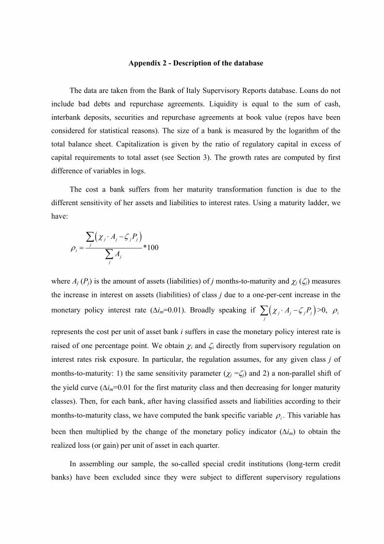
Appendix 2 - Description of the database

The data are taken from the Bank of Italy Supervisory Reports database. Loans do not

include bad debts and repurchase agreements. Liquidity is equal to the sum of cash,

interbank deposits, securities and repurchase agreements at book value (repos have been

considered for statistical reasons). The size of a bank is measured by the logarithm of the

total balance sheet. Capitalization is given by the ratio of regulatory capital in excess of

capital requirements to total asset (see Section 3). The growth rates are computed by first

difference of variables in logs.

The cost a bank suffers from her maturity transformation function is due to the

different sensitivity of her assets and liabilities to interest rates. Using a maturity ladder, we

have:

( )*100

j j j jj

ij

j

A P

A

χ ζρ

⋅ −=

∑∑

where Aj (Pj) is the amount of assets (liabilities) of j months-to-maturity and χj (ζj) measures

the increase in interest on assets (liabilities) of class j due to a one-per-cent increase in the

monetary policy interest rate (∆im=0.01). Broadly speaking if ( )j j j jj

A Pχ ζ⋅ −∑ >0, iρ

represents the cost per unit of asset bank i suffers in case the monetary policy interest rate is

raised of one percentage point. We obtain χi and ζi directly from supervisory regulation on

interest rates risk exposure. In particular, the regulation assumes, for any given class j of

months-to-maturity: 1) the same sensitivity parameter (χj =ζj) and 2) a non-parallel shift of

the yield curve (∆im=0.01 for the first maturity class and then decreasing for longer maturity

classes). Then, for each bank, after having classified assets and liabilities according to their

months-to-maturity class, we have computed the bank specific variable iρ . This variable has

been then multiplied by the change of the monetary policy indicator (∆im) to obtain the

realized loss (or gain) per unit of asset in each quarter.

In assembling our sample, the so-called special credit institutions (long-term credit

banks) have been excluded since they were subject to different supervisory regulations

34

regarding the maturity range of their assets and liabilities. Nevertheless, special long-term

credit sections of commercial banks have been considered part of the banks to which they

belonged. Foreign banks are also excluded as they are subject to their home country control.

Particular attention has been paid to mergers. In practice, it is assumed that these took

place at the beginning of the sample period, summing the balance-sheet items of the merging

parties. For example, if bank A is incorporated by bank B at time t, bank B is reconstructed

backward as the sum of the merging banks before the merger.

Data are quarterly and are not seasonally adjusted. Three seasonal dummies and a

constant are also included. For cleaning, all observations for which lending, liquidity and

total assets are equal to or less than zero were excluded. After this treatment, the sample

includes 691 banks and 26,108 observations.

An observation has been defined as an outlier if it lies within the top or bottom

percentile of the distribution of the quarterly growth rate of lending. If a bank has an outlier

in the quarterly growth rate of lending it is completely removed from the sample. The final

dataset was composed of 558 banks (20,727 observations).

A “lowly capitalized” bank has a capital ratio equal to the average capital ratio below

the 10th percentile, a “highly capitalized” bank, that of the banks above the 90th percentile.

Since the characteristics of each bank could change over time, percentiles have been worked

out on mean values.

References

Allen F. and D. Gale (1997), “Financial Markets, Intermediaries, and Intertemporal Smoothing”, Journal of Political Economy, 3, 523-546.

Altunbas, Y., O. Fazylow and Molyneux, P. (2002), “Evidence on the Bank Lending Channel in Europe”, Journal of Banking and Finance, forthcoming.

Angeloni, I., L. Buttiglione, G. Ferri and E. Gaiotti (1995), “The Credit Channel of Monetary Policy across Heterogeneous Banks: The Case of Italy”, Banca d’Italia, Temi di discussione, No. 256.

Bagliano, F.C. and C.A. Favero (1995), “The Credit Channel of Monetary Transmission: The Case of Italy”, Università Cattolica del Sacro Cuore, Milano, mimeo.

Barrios, V.E. and J.M. Blanco (2001), “The Effectiveness of Bank Capital Adequacy Requirements: A Theoretical and Empirical Approach”, IRES, Discussion Paper, No.1.

Basle Committee on Banking Supervision (1988), “International Convergence of Capital Measurements and Capital Standards ”, July.

Basle Committee on Banking Supervision (1999), “Capital Requirements and Bank Behaviour: the Impact of the Basle Accord”, Working Paper No. 1, April.

Bernanke, B. and A.S. Blinder (1988), “Is it Money or Credit, or Both or Neither? Credit, Money and Aggregate Demand”, American Economic Review, Vol. 78, No. 2, pp. 435-9. Paper and Proceedings of the One-Hundredth Annual Meeting of the American Economic Association.

Besanko, D. and G. Kanatas (1996), “The Regulation of Bank Capital: Do Capital Standards Promote Bank Safety?”, Journal of Financial Intermediation, 5, 160-183.

Bolton, P. and X. Freixas (2001), “Corporate Finance and the Monetary Transmission Mechanism”, CEPR, Discussion Paper Series, No. 2982.

Buttiglione, L. and G. Ferri (1994), “Monetary Policy Transmission via Lending Rates in Italy: Any Lessons from Recent Experience?”, Banca d’Italia, Temi di discussione, No. 224.

Buttiglione, L., P. Del Giovane and E. Gaiotti (1997), “The Role of Different Central Bank Rates in the Transmission of Monetary Policy”, Banca d’Italia, Temi di discussione, No. 305.

Calem, P. and R. Rob (1999), “The Impact of Capital-Based Regulation on Bank Risk Taking”, Journal of Financial Intermediation, Vol. 8, pp.317-352.

Calomiris, C. W. and G.R. Hubbard, (1995), “Internal Finance and Investment: Evidence from the Undistributed Profit Tax of 1936-37”, Journal of Business, Vol. 68. No. 4.

Calza, A., Gartner C. and Sousa J. (2001), “Modelling the Demand for Loans to the Private Sector in the Euro Area”, ECB, Working Paper, No. 55.

Chiades, P. and L. Gambacorta (2003), “The Bernanke and Blinder Model in an Open Economy: the Italian Case”, German Economic Review, forthcoming.

36

Coco, G. (2000), “On the Use of Collateral”, Journal of Economic Surveys, Vol. 14, pp. 191-214.

Cornett, M. M., and H. Tehranian (1994), “An Examination of Voluntary Versus Involuntary Security Issuances by Commercial Banks: The Impact of Capital Regulations on Common Stock Returns”, Journal of Financial Economics, Vol. 35, pp. 99-122.

de Bondt, G. (1999), “Banks and Monetary Transmission in Europe: Empirical Evidence”, BNL Quarterly Review, Vol. 52, No. 209, pp. 149-68.

Dewatripont, M. and J. Tirole (1994), The Prudential Regulation of Banks, Cambridge, Massachusetts, MIT Press.

Ehrmann, M., L. Gambacorta, J. Martinez Pagés, P. Sevestre and A. Worms (2003), “Financial Systems and the Role of Banks in Monetary Policy Transmission in the Euro Area”, in Angeloni, I., A. Kashyap and B. Mojon, Monetary Policy Transmission in the Euro Area, Cambridge, Cambridge University Press.

Ellis, D.M. and M.J. Flannery (1992), “Risk Premia in Large CD Rates: Time Series Evidence on Market Discipline”, Journal of Monetary Economics, Vol. 30, pp.481-502.

Fanelli, L. and P. Paruolo (1999), “New Evidence on the Transmission Mechanisms of Monetary Policy in Italy before Stage III of European Monetary Union” presented at the 9th Sadiba Conference “Ricerche Quantitative per la Politica Economica”, Perugia, December.

Favero, C. A., L. Flabbi and F. Giavazzi (1999), “The Transmission Mechanism of Monetary Policy in Europe: Evidence from Banks' Balance Sheets”, CEPR Discussion Paper, No. 2303.

Flannery, M.J. (1989), “Capital Regulation and Insured Banks’ Choice of Individual Loan Default Risks”, Journal of Monetary Economics, Vol. 24, pp. 235-58.

Flannery, M.J. and Sorescu S.M. (1996), “Evidence of Market Discipline in Subordinated Debenture Yields: 1983-1991”, Journal of Finance, Vol. 51, pp. 1347-77.

Friedman, B. (1991), “Comment on ‘The Credit Crunch’” by Bernanke B.S. and C.S. Lown, Brooking Papers on Economic Activity, No. 2, pp. 240-7.

Furfine, C. (2000), Evidence on the Response of US Banks to Changes in Capital Requirements, BIS Working Papers, No. 88.

Gambacorta, L. (2001), “Bank Specific Characteristics and Monetary Policy Transmission: the Case of Italy”, Temi di discussione, Banca d’Italia, No. 430.

Gennotte, G. and Pyle D. (1991), “Capital Controls and Bank Risk”, Journal of Banking and Finance, Vol. 15, pp. 805-24.

Giammarino, R.M., T.R. Lewis and D. Sappington (1993), “An Incentive Approach to Banking Regulation”, Journal of Finance, Vol. 48, No. 4, pp. 1523-42.

Gorton, G. and R. Rosen (1996), “Corporate Control, Portfolio Choice, and the Decline of Banking”, Journal of Finance, Vol. 50, pp.1377-1420.

37

Green C.J. (1998), “Banks as Interest Rate Managers”, Journal of Financial Services Research, Vol. 14, No. 3, pp. 189-208.

Hancock, D., J.A. Laing and J.A. Wilcox (1995), “Bank Capital Shocks: Dynamic Effects on Securities, Loans, and Capital”, Journal of Banking and Finance, Vol. 19, pp.661-77.

Hellman, T., K. Murdock, and J. Stiglitz (2000), “Liberalization, Moral Hazard in Banking, and Prudential Regulation: Are Capital Requirement Enough?”, American Economic Review, March, pp. 147-65.

Houston, J. and C. James (1998), “Do Bank Internal Markets Promote Lending?”, Journal of Banking and Finance, No.6-8, pp.899-918.

Keeley, M.C. (1990), “Deposit Insurance, Risk and Market Power in Banking”, American Economic Review, Vol. 80, pp. 305-60.

Kim, D. and A. M. Santomero (1988), “Risk in Banking and Capital Regulation”, Journal of Finance, Vol. 43, pp.1219-33.

King, S.K. (2002), “A Credit Channel in Europe: Evidence from Bank’s Balance Sheets”, University of California, Davis, mimeo.

Kishan, R. P. and T. P. Opiela (2000), “Bank Size, Bank Capital and the Bank Lending Channel”, Journal of Money, Credit and Banking, Vol. 32, No. 1, pp. 121-41.

Koehn, M. and A. M. Santomero (1980), “Regulation of Bank Capital and Portfolio Risk”, Journal of Finance, Vol. 35, pp. 1235-1244.

Kwan, S. and Eisenbeis, R. A. (1997), “Bank Risk, Capitalization, and Operating Efficiency”, Journal of Financial Service Research, Vol. 12, No. 2-3, pp. 117-31.

Leland, H. E. and Pile D. H. (1977), “Informational Asymmetries, Financial Structures and Financial Intermediation”, The Journal of Finance, Vol. 32, pp. 371-87.

Lim, G.C. (2000), “Bank Interest Rate Adjustments: Are They Asymmetric?”, The Economic Record, Vol. 77, no. 237, pp.135-147.

Myers, S.C. and N. S. Majluf (1984), “Corporate Finance and Investment Decisions when Firms Have Information that Investors Do Not Have”, Journal of Financial Economics, Vol. 13, pp.187-221.

Rao, C. R. (1973), Linear Statistical Inference and its Applications, New York, John Wiley and Sons.

Repullo, R. (2000), “Who Should Act as Lender of Last Resort? An Incomplete Contracts Model”, Journal of Money, Credit and Banking, Vol. 32, pp. 580-605.

Rime, B. (2001), “Capital Requirements and Bank Behaviour: Empirical Evidence for Switzerland”, Journal of Banking and Finance, No.4, pp.789-805.

Rochet, J. C. (1992), “Capital Requirements and the Behaviour of Commercial Banks”, European Economic Review, Vol. 36, pp.733-62.

Romer, C.D. and D.H. Romer (1990), “New Evidence on the Monetary Transmission Mechanism”, Brooking Paper on Economic Activity, No. 1, 1990, pp.149-213.

Santomero, A.M. (1984), “Modeling the Banking Firm: A Survey”, Journal of Money Credit and Banking, Vo. 16, No. 4, pp. 576-602.

38

Sheldon, G. (1996), “Capital Adequacy Rules and the Risk-Seeking Behaviour of Banks: A Firm-Level Analysis”, Swiss Journal of Economics and Statistics, Vol. 132, pp. 709-734.

Stein, J. C. (1998), “An Adverse-Selection Model of Bank Asset and Liability Management with Implications for the Transmission of Monetary Policy”, RAND Journal of Economics, Vol. 29, No. 3, pp. 466-86.

Thakor, A.V. (1996), “Capital Requirements, Monetary Policy, and Aggregate Bank Lending: Theory and Empirical Evidence”, The Journal of Finance, Vol. 51, No. 1, pp. 279-324.

Van den Heuvel, S.J. (2001a), “The Bank Capital Channel of Monetary Policy”, University of Pennsylvania, mimeo.

Van den Heuvel, S.J. (2001b), “Banking Conditions and the Effects of Monetary Policy: Evidence from U.S. States”, University of Pennsylvania, mimeo.

Van den Heuvel, S.J. (2003), “Does Bank Capital Matter for Monetary Transmission?”, FRBNY Economic Policy Review, forthcoming.

Vander Vennet, R. and Van Landshoot A. (2002), “How Do Internationalization, Diversification and Capitalization Affect Bank Credit Risk? Evidence From Bank Stock Market Returns”, paper presented at the 17th European Economic Association Annual Conference (Venice, 22-24 August).

Vlaar P.J.G. (2000), “Capital Requirements and Competition in the Banking Industry”, De Nederlandsche Bank, Research Memorandum WO&E, No. 634.

Table 1

DATA DESCRIPTION (September 2001)

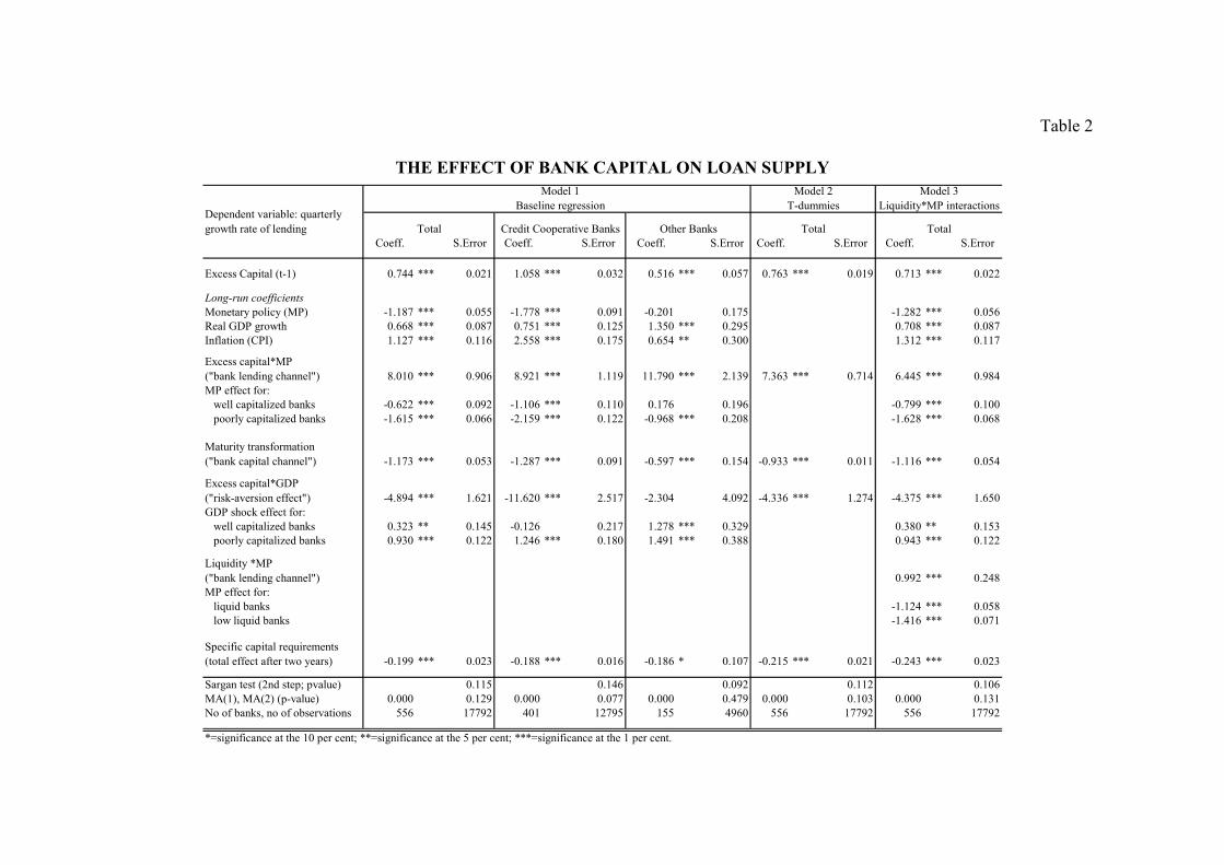
Table 2

THE EFFECT OF BANK CAPITAL ON LOAN SUPPLY

Coeff. S.Error Coeff. S.Error Coeff. S.Error Coeff. S.Error Coeff. S.Error

Excess Capital (t-1) 0.744 *** 0.021 1.058 *** 0.032 0.516 *** 0.057 0.763 *** 0.019 0.713 *** 0.022

Long-run coefficientsMonetary policy (MP) -1.187 *** 0.055 -1.778 *** 0.091 -0.201 0.175 -1.282 *** 0.056Real GDP growth 0.668 *** 0.087 0.751 *** 0.125 1.350 *** 0.295 0.708 *** 0.087Inflation (CPI) 1.127 *** 0.116 2.558 *** 0.175 0.654 ** 0.300 1.312 *** 0.117

Excess capital*MP ("bank lending channel") 8.010 *** 0.906 8.921 *** 1.119 11.790 *** 2.139 7.363 *** 0.714 6.445 *** 0.984MP effect for: well capitalized banks -0.622 *** 0.092 -1.106 *** 0.110 0.176 0.196 -0.799 *** 0.100 poorly capitalized banks -1.615 *** 0.066 -2.159 *** 0.122 -0.968 *** 0.208 -1.628 *** 0.068

Maturity transformation ("bank capital channel") -1.173 *** 0.053 -1.287 *** 0.091 -0.597 *** 0.154 -0.933 *** 0.011 -1.116 *** 0.054

Excess capital*GDP ("risk-aversion effect") -4.894 *** 1.621 -11.620 *** 2.517 -2.304 4.092 -4.336 *** 1.274 -4.375 *** 1.650GDP shock effect for: well capitalized banks 0.323 ** 0.145 -0.126 0.217 1.278 *** 0.329 0.380 ** 0.153 poorly capitalized banks 0.930 *** 0.122 1.246 *** 0.180 1.491 *** 0.388 0.943 *** 0.122

Liquidity *MP ("bank lending channel") 0.992 *** 0.248MP effect for: liquid banks -1.124 *** 0.058 low liquid banks -1.416 *** 0.071

Specific capital requirements (total effect after two years) -0.199 *** 0.023 -0.188 *** 0.016 -0.186 * 0.107 -0.215 *** 0.021 -0.243 *** 0.023

Sargan test (2nd step; pvalue) 0.115 0.146 0.092 0.112 0.106MA(1), MA(2) (p-value) 0.000 0.129 0.000 0.077 0.000 0.479 0.000 0.103 0.000 0.131No of banks, no of observations 556 17792 401 12795 155 4960 556 17792 556 17792

*=significance at the 10 per cent; **=significance at the 5 per cent; ***=significance at the 1 per cent.

Dependent variable: quarterly growth rate of lending Total Credit Cooperative Banks Other Banks

Model 1 Baseline regression

Model 2 T-dummies

Total

Model 3 Liquidity*MP interactions

Total

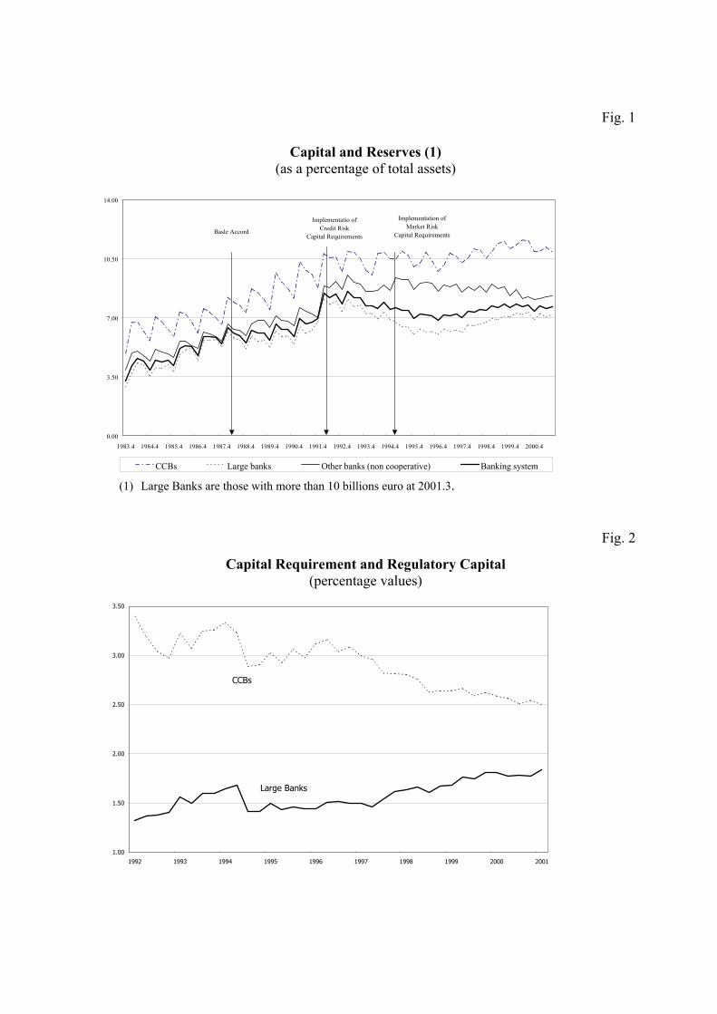
Fig. 1

Capital and Reserves (1) (as a percentage of total assets)

(1) Large Banks are those with more than 10 billions euro at 2001.3.

Fig. 2

Capital Requirement and Regulatory Capital (percentage values)

0.00

3.50

7.00

10.50

14.00

1983.4 1984.4 1985.4 1986.4 1987.4 1988.4 1989.4 1990.4 1991.4 1992.4 1993.4 1994.4 1995.4 1996.4 1997.4 1998.4 1999.4 2000.4

CCBs Large banks Other banks (non cooperative) Banking system

Basle Accord

Implementatio ofCredit Risk

Capital Requirements

Implementation ofMarket Risk

Capital Requirements

1.00

1.50

2.00

2.50

3.00

3.50

1992 1993 1994 1995 1996 1997 1998 1999 2000 2001

CCBs

Large Banks

Fig. 3

The evolution of banks’ capitalization (normalized distance from long run average capitalization, quarterly data)

Fig. 4

Maturity transformation (months-to-maturity, average)

-1.0

-0.5

0.0

0.5

1.0

1992.2 1993.2 1994.2 1995.2 1996.2 1997.2 1998.2 1999.2 2000.2 2001.2

all banks large banks other banks ccb

0

10

20

30

40

50

1992 1993 1994 1995 1996 1997 1998 1999 2000 2001

CCBsAssets

Liabilities

Assets

Liabilities

Banks