1

August 15, 2014

Bank asset reallocation and sovereign debt

Michele Fratianni* and Francesco Marchionne**

Abstract

This paper examines how banks around the world have resized and reallocated their earning assets in response to the subprime and sovereign debt crises. We focus especially on the interaction between sovereign debt and the bank asset allocation process. After the crisis we observe a general substitution away from loans and in favor of securities. Our econometric findings corroborate that banks have readjusted the composition of their assets and the overall regulatory credit risk by substituting securities for loans. Banks, furthermore, have also been sensitive to those variables that are of direct interest to the regulator. The picture that emerges is a mutual protection pact regime, in which high-debt governments exert pressure on banks-- either through the regulatory system or through moral suasion-- to privilege the purchase of government securities over credit to the private sector in exchange for receiving protection against default. Key words: crisis, loans, regulator, securities, mutual protection pact JEL Classification: G01, G11, G21, G28. * Indiana University, Kelley School of Business, Bloomington, Indiana 47405, USA; Università Politecnica delle Marche, Ancona (Italy; Money and Finance Research Group (MoFiR); fratiann@indiana.edu ** Nottingham Trent University, Nottingham Business School, NG1 4BU, Nottingham, UK; Money and Finance Research Group (MoFiR); francesco.marchionne@ntu.ac.uk. Acknowledgement: This paper was written while Marchionne was a Visiting Fellow at the Indiana University Kelley School of Business; thanks are expressed to the hosting institution.

2

I. INTRODUCTION

This paper examines how banks around the world have resized and reallocated their earning

assets in response to the subprime and sovereign debt crises. In particular, we focus on the

interaction between sovereign debt and bank asset allocation process.

The first impact of the subprime financial crisis occurred through the re-pricing of

risk across a variety of assets and the shrinking of balance sheets. Recapitalization was

aggressively pursued from the second half of 2007 through September 2008, when global

banks raised $430 billion of fresh capital (IMF 2008: 22). Then, recapitalization became

increasingly costly, and leverage was effected by selling assets in illiquid markets.1 Thus, in

the absence of fresh capital and without significant profits to retire debt in the short run, the

de-leveraging process necessarily implied distress sales and falling asset values (Adrian and

Shin 2008, Figure 2.5). The rapidly rising risk aversion of the public, fed by bad news and the

thick fog of asymmetric information, pushed financial institutions to compress leverage

quickly. According to Kollmann (2013), during the 2007–09 recession banking shocks

accounted for about 15 percent of the fall in the US and the Eurozone GDP. The failure of

Lehman Brothers on September 15, 2008 prompted governments to implement vast and

costly rescue operations of their banking system (Fratianni and Marchionne 2013). Banks that

received government assistance bought valuable time to restructure. Banks that did not

receive assistance had to adjust more quickly.

Bank bailouts shifted risk from banks to governments (Acharya et al. 2014;

Hryckiewicz 2014).2 The sovereign debt crisis of 2010 in the Eurozone and the consequent

rise in spreads of government yields in the Southern countries relative to Germany’s provided

undercapitalized banks an opportunity to engage in gamble-for-resurrection strategies.

1 With higher information asymmetries due to the crisis, investors are more reluctant to invest in bank equities. On the other hand, government-funded rescue plans raise banks’ appetite for risk. In sum, adverse selection and moral hazard work towards undercapitalization. 2 For the countries of the Eurozone as a group, government gross debt rose from €6,493 billion in 2008 to €9.119 billion in 2013 (IMF, WEO database).

3

Acharya and Steffen (2013) present evidence of this strategy in which liquid government

securities receive a preferential treatment, relative to bank loans, in capital regulatory risk

weights and in government guarantees that make them an ideal collateral to obtain cheap

central-bank funding. This phenomenon found its zenith when the South of the Eurozone,

facing a sudden stop and later a reversal in capital flows, became disconnected from the

money market in the North of the Eurozone.3 The European Central Bank (ECB) launched in

2011 and 2012 two rounds of exceptional lending to banks at cheap rates to ease the

fragmentation of the inter-bank market.4 The shift from bank loans to securities occurred with

a home bias (Levy and Levy 2014, Popov and van Horen 2013). In an investigation of this

bias, Battistini et al. (2013) suggest two non-traditional reasons for this phenomenon. The

first is that high-risk governments may exert pressure on domestic banks to buy more

government debt; this pressure is part of an implicit mutual protection pact between banks

and the sovereign. The second is that domestic government securities are a better edge than

foreign euro-denominated securities should the country re-introduce a national currency.

Whether with or without a home bias, undercapitalized banks raise the share of their assets in

securities at the expense of private-sector credit. The implication is a displacement of

investments, as in the model by Broner et al (2013) where the sovereign, in turbulent times,

issues high-interest rate debt that is so attractive to crowd out alternative forms of debt.

The nexus between banks and sovereign can generate negative feedbacks (vicious

circles). The traditional view has it that a credit crunch worsens borrowers’ prospect of

repaying outstanding loans, making banks riskier and necessitating further de-leveraging and

de-risking. A different explanation is offered by Angelini et al. (2014): “the risk of a

government’s insolvency is a factor that permeates the entire national economy and is

3 On sudden stops of capital flows, see Merler and Pisani-Ferry (2012); on the underlying factors of rising spreads in the Eurozone, see Alessandrini et al. (2014). 4 This exceptional form of lending is known as long-term refinancing operations which had a maturity of 3 years and carried an interest rate of one percent. €489 billion were utilized in December of 2011 and €529 billion in February of 2012. Italian banks absorbed €281 billion and Spanish banks €365 billion.

4

transmitted to all of the country’s private institutions, not just to the banks; second, that the

recent expansion of banks’ government securities portfolios is a consequence, not a cause, of

the crisis...” (p. 28). Both interpretations predict a shift towards government securities in

banks’ portfolio during a sovereign debt crisis.

There are a few recent studies on this topic. Sandleris (2014) develops a theoretical

model showing that sovereign defaults can lead to a decline in foreign and domestic credit to

the domestic private sector, even if domestic agents do not hold sovereign debt; stronger

domestic financial institutions can amplify this effect. Acharya et al. (2014) model and test a

two-way feedback between sovereign risk and bank credit risk and obtain that the positive

relationship between public debt-to-GDP ratios and sovereign CDS premia is larger in

countries with pre-bailout highly stressed banking sectors and higher debt ratios. Using

dynamic panel methods, Buch et al. (2010) show that banks’ first reaction to a domestic

shock is to reduce foreign assets. Adelino and Ferreira (2014) apply difference-in-difference

analysis to test the effectiveness of ceiling policies on banks’ holdings of sovereign debt set

by credit rating agencies. The authors find that sovereign downgrades by the agencies lead to

a reduction of 30 percent in loan amounts (and a 15-50 basis points increase in loan spreads)

for those banks close to the ceiling. To be noted, these studies focus on sudden macro shocks,

whereas we emphasize banks’ continuous portfolio adjustment.

With this background, our paper focuses on the interaction between sovereign debt

and bank asset allocation process during the period 2005-2012, eight years that include four

pre-crisis years and four crisis years. Data before 2005 are incomplete and available only for

a few countries; the same is true for data after 2012. Sovereign debt is a privileged asset in

that it does not absorb capital, unlike loans to the private sector. It can also be easily sold in

liquid markets and is highly collateralizable to obtain monetary base from the central bank.

All of these characteristics are observable and known and stem in large part from the

5

financial regulator (in essence either the government or the central bank) having set formal

and observable rules. But the regulator also uses informal and unobservable rules in

influencing banks’ decisions concerning asset allocation. These rules respond to the trade-off

the regulator faces between systemic risk reduction and public debt financing; and the

intensity of the trade-off rises during a financial crisis. The value of sovereign debt as a

proportion of national GDP is used as a proxy of the overall impact on the banking system of

both observed and unobservable rules. Our empirical specification will test to what extent

loans and securities behave as substitutes; whether the asset allocation process favors

securities and the existence of a “mutual protection pact” between banks and government;

and whether banks are sensitive to the observed variables that are of direct interest to the

regulator.

Our findings show that banks can readjust the composition of their assets and the

overall regulatory credit risk by substituting securities for loans, and are sensitive to the

variables that are of direct interest to the regulator. These findings are also consistent with a

mutual protection pact regime, in which high-debt governments exert pressure on banks

(either through the regulatory system or through moral suasion) to privilege the purchase of

government securities over credit to the private sector in exchange for protecting the banking

system. The quality of our findings is strengthened by the large dataset we have used. While

previous studies have focused on specific institutions, typically large banks, ours

encompasses the universe of the available categories of banks; and to our knowledge, this is

the first paper to do so.

The structure of the paper is as follows. Section II presents our empirical strategy and

the testable hypotheses. Section III deals with data and descriptive statistics. Virtually all of

our data come from Bankscope, which have a high proportion of missing values and outliers.

Since these aspects tend to bias coefficients’ estimates and generate unstable results, we have

6

spent considerable resources in cleaning the data. We present and discuss our empirical

findings in Section IV and their robustness in Section V. In recognition of the likelihood that

our data-cleaning procedure might have not been able to eradicate completely the outlier

problem, we also apply regression analyses that are robust to such anomaly. The last section

of the paper sums up the salient findings, their policy implications and themes for future

research.

II. EMPIRICAL SPECIFICATION

Our empirical approach consists of two simultaneous equations, one explaining gross loans

and the other total securities.5 The specification captures demand conditions, supply

constraints, and the influence of the country’s bank regulator-supervisor (simply the

regulator). Banks exploit market demand to seize profitable opportunities, but face supply

constraints resulting from the limitations of their financial structure. The sensitivity of bank

loans and securities to demand shocks is used as a measure of the bank’s ability to seize

market opportunities (Gomez Meja et al., 2007). In light of the fact that revenue-oriented

strategies are inherently risky, the regulator sets rules to reduce systemic risk (for our

purposes we concentrate on credit risk) and limit the degree of moral hazard. Rules can be

formal and observable and/or informal and unobservable to the market. Capital requirements

are an example of formal and observable rules: banks must adhere to keep a minimum ratio

of bank capital to risk-weighted assets, where the weight is positive for bank loans and zero

for government securities. The impact of bank inspections and moral suasion on banks’

decisions are an example of an informal and unobservable interventions. During economic

downturns, the regulator faces a trade-off between systemic risk reduction and public debt

5 The number of observations on holdings of government securities is approximately one half of the observations on holdings of total securities in Bankscope. Considering that on average government securities represent 44.34 percent share of total securities and that their correlation coefficient is 66.42 percent, we have used the latter as a proxy of the former.

7

financing. While public debt is formally set to have a zero credit risk, in reality it is not.

Aware of the difference between formal rules and markets’ perception, the regulator can use

moral suasion to induce banks to alter asset allocation in favor of securities, thus influencing

the degree of moral hazard in banks. The regulator can also influence banks’ decisions

concerning de-leveraging and asset allocation by being tougher or easier during bank

inspections. If he is tougher, he will force banks to make upward adjustments in non-

performing loans; the opposite is true if he is more tolerant. Either way, the regulator will

affect bank profitability and the level of bank capital, and consequently banks’ decisions on

de-leveraging and asset allocation.

The structure of each equation is somewhat reminiscent of a Capital Asset Price Model

(CAPM) used in the economics of industrial organization; see Bertrand et al. (2002) and

Sraer and Thesmar (2007).6 There, the firm’s sales growth rate depends on the industry’s

growth rate, firm-specific characteristics and country-specific characteristics. The demand of

firm i is proxied by industry’s sales. This approach has two advantages. The first is a

parsimonious use of data, as the demand is determined endogenously exploiting information

provided by the dataset. It also reduces the difficulty of integrating alternative data sets with

bank accounting data, in particular specific series like bank loans and securities. The second

is that the model uses only current variables rather than current and lagged variables. With

lagged variables one faces a higher risk of having missing values and ending up with a

selection bias. In sum, our model specification is economical in the use of data and more

efficient in handling datasets with many missing values.

We adapt the industrial organization framework to the banking sector in four ways. First,

we replace firm’s sales with bank’s growth rate of loans, ��, in equation (1) and bank’s

6 Bertrand et al. (2002) use variation in mean industry performance as a source of profit shocks in the single firm to trace the propagation of shocks through a business group. Sraer and Thesmar (2007) estimate a fixed effect model, where single firm sensitivity is identified by the correlation between the changes in log sales and log employment. In both the models, industry shocks provide an ideal candidate to measure firm sensitivity since they affect individual firms but are – to a large extent – beyond the control of individual firms.

8

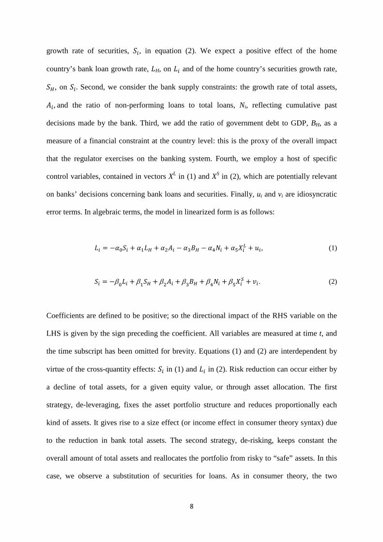
growth rate of securities, ��, in equation (2). We expect a positive effect of the home

country’s bank loan growth rate, �H, on �� and of the home country’s securities growth rate,

��, on ��. Second, we consider the bank supply constraints: the growth rate of total assets,

�� ,and the ratio of non-performing loans to total loans, Ni, reflecting cumulative past

decisions made by the bank. Third, we add the ratio of government debt to GDP, BH, as a

measure of a financial constraint at the country level: this is the proxy of the overall impact

that the regulator exercises on the banking system. Fourth, we employ a host of specific

control variables, contained in vectors XL in (1) and XS in (2), which are potentially relevant

on banks’ decisions concerning bank loans and securities. Finally, ui and vi are idiosyncratic

error terms. In algebraic terms, the model in linearized form is as follows:

�� = −���� + ���� + ���� − ���� − ����+����� + ��, (1)

�� = −β��� + β

��� + β

��� + β

��� + β

��� + β

���� + ��. (2)

Coefficients are defined to be positive; so the directional impact of the RHS variable on the

LHS is given by the sign preceding the coefficient. All variables are measured at time t, and

the time subscript has been omitted for brevity. Equations (1) and (2) are interdependent by

virtue of the cross-quantity effects: �� in (1) and �� in (2). Risk reduction can occur either by

a decline of total assets, for a given equity value, or through asset allocation. The first

strategy, de-leveraging, fixes the asset portfolio structure and reduces proportionally each

kind of assets. It gives rise to a size effect (or income effect in consumer theory syntax) due

to the reduction in bank total assets. The second strategy, de-risking, keeps constant the

overall amount of total assets and reallocates the portfolio from risky to “safe” assets. In this

case, we observe a substitution of securities for loans. As in consumer theory, the two

9

strategies are complementary and any combination of size and substitution effects is

empirically possible.

To reduce systemic risk, regulators set observable time-invariant rules (e.g., capital

requirements) aimed at preventing bank insolvency. But, as we have noted, regulators also

use discretionary power to enforce largely unobservable time-varying rules, which better

exploit the changing trade-offs over the business cycle between bank credit growth and bank

safety. We assume that banks adopt a pecking order when coping with a riskier environment,

such as selling assets in preference of raising more costly capital (Hyun and Rhee 2011) and

reallocating assets in preference of reducing total assets that would entail capital losses from

the sale of illiquid assets. The higher flexibility of the reallocation strategy avoids the

realization of losses while gambling for a resurrection of the market value of the unsold

assets. On the other hand, a reallocation strategy is more complex and takes more time than a

total asset reduction and may not be a viable option when the required risk reduction is

intense and fast.

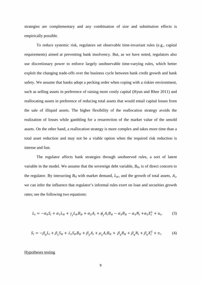
The regulator affects bank strategies through unobserved rules, a sort of latent

variable in the model. We assume that the sovereign debt variable, BH, is of direct concern to

the regulator. By interacting BH with market demand, ��, and the growth of total assets, �� ,

we can infer the influence that regulator’s informal rules exert on loan and securities growth

rates; see the following two equations:

�� = −���� + ���� + γ����� + ���� + φ

����� − ���� − ����+����

� + ��, (3)

�� = −β��� + β

��� + λ����� + β

��� + µ

����� + β

��� + β

��� + β

���� + ��. (4)

Hypotheses testing

10

Using equations (1) and (2) we can test several hypotheses. The first is that loans and

securities are not substitutable, namely H10: −�� = −β�= 0,against the alternative that the

equations are linked together, H1a: −�� < 0 and −β�< 0. The second is that changes in

total assets affect proportionally Li and Si, namely that H20: �� = β�= 1, against the

alternative hypothesis that asset reallocation favors securities, i.e., H2a: �� < β�. The third

deals with the regulator and his potential influence on bank’s decisions. Neutrality with

respect to government debt implies H30: −�� = −β�= 0, against the alternative of a mutual

protection pact that implies instead an asset reallocation in favor of securities, H3a: −�� < 0

and −β�> 0. Finally, we can test an additional hypothesis using equations (3) and (4). Banks

are insensitive to the observed variables that are of direct interest to the regulator in the sense

that changes in demand and in total assets do not interact with the sovereign debt variable,

H40: γ� =φ�= 0 and λ� = µ

�= 0, against the alternative that the interaction is not zero.

Table 1 summarizes our testable hypotheses.

[Insert Table 1 here]

III. DATA AND DESCRIPTIVE STATISTICS

Our data sources are Bankscope and the World Economic Outlook of the International

Monetary Fund (IMF) covering the period from 2004 to 2012. From Bankscope we have

obtained yearly consolidated accounting data for all financial institutions in 43 countries, 34

of which developed industrial countries (i.e., OECD countries) and nine developing

countries.7 Several different financial statements may be available for a given bank in a given

reporting period (e.g., subsidiaries, cross-border banks, etc.). This requires that rules must be

7 The 34 OECD countries are: Australia, Austria, Belgium, Canada, Chile, Czech Republic, Denmark, Estonia, Finland, France, Germany, Greece, Hungary, Korea, Iceland, Ireland, Israel, Italy, Japan, Luxemburg, Mexico, Netherlands, New Zealand, Norway, Poland, Portugal, Slovakia, Slovenia, Spain, Sweden, Switzerland, Turkey, United Kingdom, and United States. The nine developing countries included in our sample are: Brazil, China, Hong Kong, India, Indonesia, Philippines, Russian Federation, Singapore, and Taiwan.

11

defined for selecting and merging these statements to obtain a unique time series for each

institution.8 Our initial dataset consists of 197,721 observations and 21,969 banks. The term

“bank” include six types of financial institutions: bank holding and holding companies,

commercial banks, cooperative banks, investment banks, real estate and mortgage banks, and

savings banks. All of them hold loans and securities and can effect both a de-leveraging and

de-risking strategy. The market growth rate of loans and securities was computed using all

financial entities available in Bankscope, rather than the six categories of banks in our

sample; this produces a measure of market changes that is independent (and unbiased) of the

holder of loans and securities.

Data treatment

The Bankscope data contain many outliers, not only in a statistical sense but also in an

economic sense. The data need to be cleaned from these anomalies. Robust statistical

methods that identify “outlyingness” relax the homogeneity assumption that all observations

fit a given model. These methods, however, have not been widely adopted because the outlier

identification is hidden within the black box of the estimation method. The metric of

“outlyingness” is based on a measure of discrepancy from a specific model that fits the data.

But, in a more realistic situation of multiple outliers the, “outlyingness” metric may be

contaminated by an unidentified outlier; see Billor et al. (2000) for details. Thus, we take a

different approach in cleaning the data; this approach consists of three steps.

In the first step, we identify multiple outliers using the BACON (blocked adaptive

computationally efficient outlier nominators) algorithm proposed by Billor et al. (2000). This 8 The primary statement is labelled “Institution” by Bankscope. In general, this is a consolidated statement (C1, C2), and only in the few cases where a bank does not publish annual reports on a consolidated basis we use an unconsolidated version (U1). Bankscope has six codes for consolidation (C2, C1, C* and U2, U1, U*), where C indicates a consolidated and U denotes an unconsolidated statement. The extension “2” indicates that both a consolidated and an unconsolidated statement exist for a bank (codes C2 and U2) at some point of time. Accordingly, the codes C1 and U1 indicate that no companion statement exists. C* and U* indicate that additional statements have been filed. This leads to the following seniority ranking of statements filed (assuming that consolidated statements represent the most senior information available): C2\C1 > C* > U1 > U* > U2.

12

algorithm works with iterative estimates and starts with an initial basic subset of “clean”

observations and strikes a balance “...between affine equivariance and robustness” (Billor et

al 2000: 296).9 Unlike other approaches, this method identifies outliers hidden in the standard

95% confidence interval. Furthermore, it is relatively insensitive to the starting point and

detects multiple outliers with a modest computational cost (i.e., as low as four repetitions of

the underlying fitting method).10 For these reasons, it is practical with our large dataset.

Outliers detected by the BACON algorithm are treated as systematic errors and the record in

which they appear is removed from the dataset because of the contamination risk of the

outlier metric.

The second step deals with implausible negative items in the balance sheet (e.g.,

negative equity value and equity-to-total-assets ratios larger than 100 percent). We replace

these anomalies with missing values under the assumption that those observations are

idiosyncratic and do not cross correlate with other data entries for the same bank at a given

time period. If they were correlated and thus systematic, we would have eliminated the entire

record of bank i at time t. Given that the NEG procedure removes only negative values, the

treated distribution accentuates its right skewness, which, in turn, makes it necessary a further

detection method to identify right-side outliers.

The third step treats extreme outliers defined as � < �1 − 3 ∗ "� and � > �1 + 3 ∗

"�, where x is the treated variables, Q1 = 1st quartile of the frequency distribution, Q3 = 3rd

quartile, and IQ = inter-quartile difference. Given that most of our variables have a right-

9 An estimator, T, is affine equivariant if and only if T(XA + b) = T(X)A + b for any vector b and non-singular matrix A. Affine equivariance is a desirable but arduous property in the sense that a robust regression or the nomination of outliers should not depend on the location, scale, or orientation of the data. BACON selects a small subset of observations based on Mahalanobis distances (equivariance) or distances from coordinate-wise medians (robustness). Moving from this starting point, it identifies interactively new sets of central observations with similar mean and covariance matrix, drifting toward the center when the subset of observations is not near enough to the center of the non-outlying data. As the basic subset grows in size, its mean and covariance matrix become more stable, preserving the initial equivariance and robustness; for more details, see Billor et al. (2000). 10 For multivariate data, BACON is computationally more efficient and more performing multiple outlier detection method than the brute-force search, minimum volume ellipsoid (Rousseeuw and van Zomeren 1990), minimum covariance determinant (Rousseeuw and van Driessen 1999), and their more recent improvements.

13

skewed frequency distribution and our treatment of negative values, the inter-quartile

difference range procedure (IQR) detects outliers on the right side of the distribution. Again,

we consider anomalous values as idiosyncratic errors and in the data are replaced with

missing values.

The three steps were first applied to the original variables in level and then to the

computed rates of growth and ratios. The only exception is the negative-value correction for

growth rates: in this case, the frequency distributions are normal and the inter-quartile

differences impact symmetrically on both sides of the distribution.

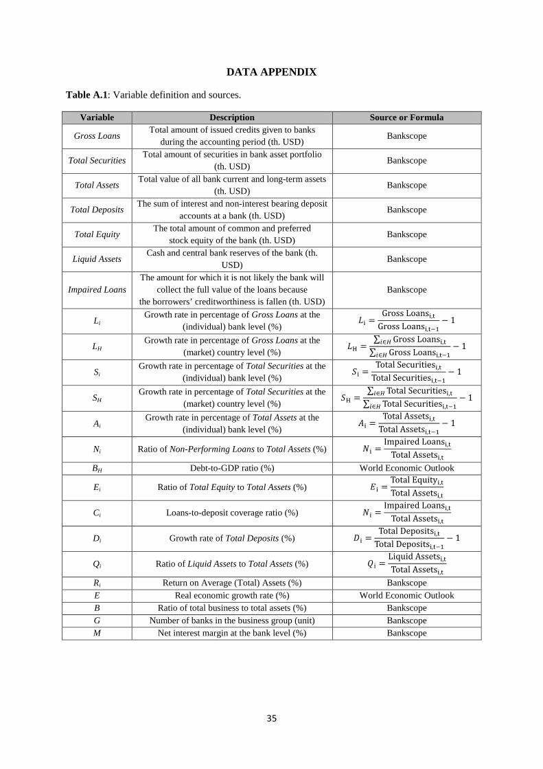
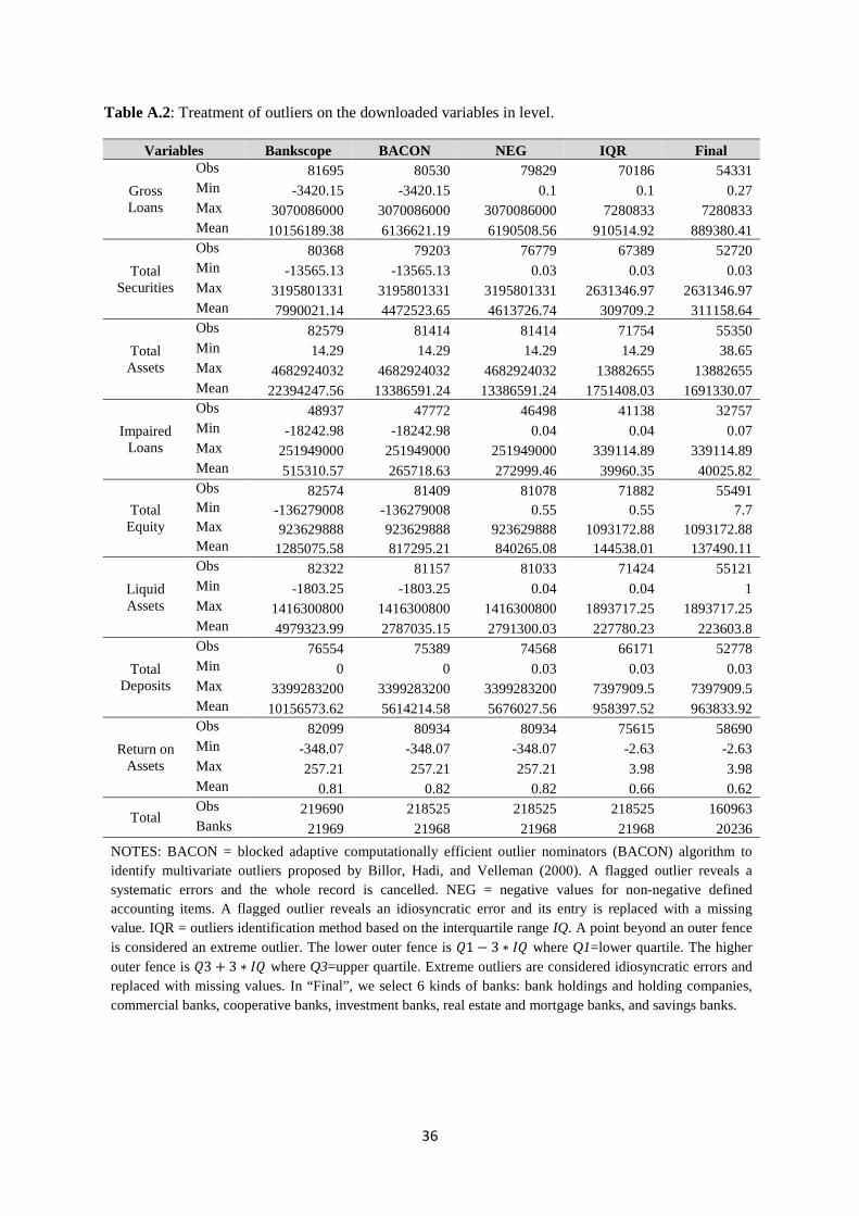
The reader can find in the Appendix detailed information on data and their treatment:

Table A.1 shows the list of variables, their description and sources; Tables A.2 and A.3

present the results from the treatment on the original variables in level and on the computed

rates of growth and ratios, respectively. We recall that BACON removes the affected records

from the dataset, whereas NEG and IQR replace data entries with missing values. The

presence of outliers is evident from the range of the original variables shown in Table A.2

(column “Bankscope”). This is further evidenced in the box plots of Figure A.1. BACON

detects 1,165 anomalous records. NEG and IRQ procedures identify a much higher number

of outliers for all variables, in particular for our two variables of interest, gross loans (10,344)

and total securities (11,841). The bank selection criterion reduces the sample by 15-20

percent.

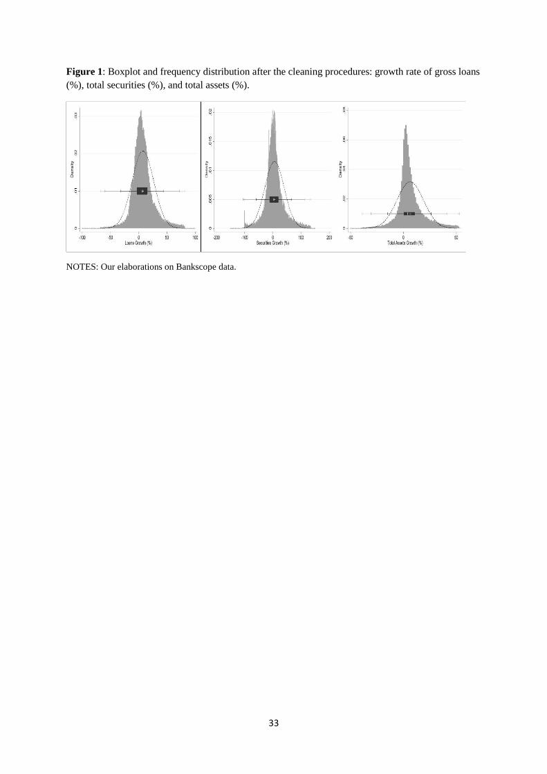
Figure 1 shows the impact of our cleaning procedure on the frequency distributions of

three critical variables. Gross loans, total securities, and total assets expressed in growth rates

resemble a normal distribution, except for evidence of leptokurtosis due to the presence of

outliers. A flatter leptokurtic distribution implies a higher variance. The black line in the

boxplots shows the range between the inner fences (i.e., between �1 − 1.5 ∗ "� and �3 +

1.5 ∗ "�); the dark grey line the range between the outer fences (i.e., between �1 − 3 ∗ "�

14

and �3 + 3 ∗ "�); and the light grey the range between the maximum and minimum points.

The identification of severe outliers can be obtained by difference.

[Insert Figure 1]

To give a measure of the impact of the cleaning and selection process on growth rates

and on ratios, consider that the maximum value of gross loans and total securities is

1,808,766 and 60,486,568 percent, respectively, before the treatment and 81.76 and 134.57

percent after. The treatment reduces the number of observations considerably, in a range

contained between 25 to 75 percent depending on the variable in question; see Appendix for

more details.

Descriptive statistics

Panel A of Table 2 presents descriptive statistics after the cleaning procedure.11 Four points

are worth making. The first is that our dataset consists of 20,236 banks, but we lose more

than two thirds of the observations as missing values; as an example, out of potential 160,963

observations for gross loans 54,331 remain usable. The second is that the wide dispersion of

these variables and the right-skewness of the frequency distributions (e.g. 2.44 for gross

loans, 2.43 for total securities, and 2.46 for total assets) indicate a further potential problem

with outliers. The third is that all variables are leptokurtic, in particular gross loans (8.89),

total securities (8.69) and total assets (8.94). The evidence of leptokurtosis and skewness

suggest the use of growth rates to handle normally distributed variables. Finally, dummy

variables show that 59 percent of observations come from commercial banks and 43 percent

from banks adopting a regulatory accounting standard. These statistics corroborate the

prevailing view that the introduction of a new regulatory system during a financial crisis is

relatively slow moving.

11 Growth rates and computed ratios are not reported for brevity.

15

[Insert Table 2 here]

Panel B of Table 2 presents descriptive statistics for the only country-level variable

used in our study, the ratio of gross government debt to GDP ratio.12 Also this ratio shows

wide dispersion, right-skewness and leptokurtosis. These statistical phenomena reflect, not

only the mix of highly indebted developed countries with lowly indebted developing

countries, but also the jump in the debt-to-GDP ratio that has occurred as a result of the last

financial and sovereign debt crisis.

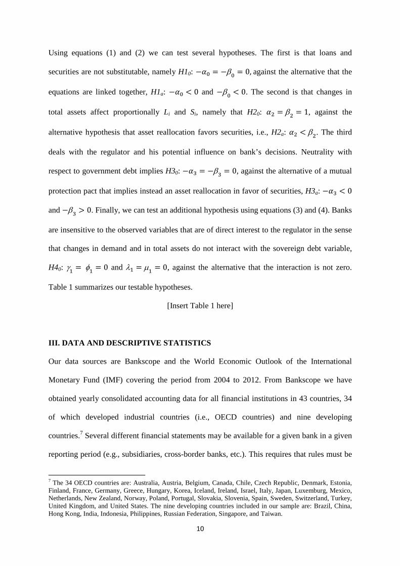
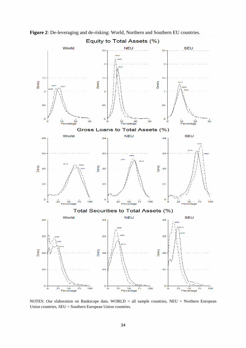
Figure 2 shows the movement over the sample period of three critical frequency

distributions. For improved visual clarity, we plot the distribution in the pre-crisis year of

2005, in the peak crisis year of 2008, and in the last available year of 2012. The leverage ratio

at the world level rises until 2008 and declines during the crisis.13 But in Europe, one can

identify an asymmetry between Northern EU countries (NEU) where the leverage ratio is

continuously decreasing, and Southern EU countries (SEU) where it is increasing.14

In other words, the expected process of de-leveraging following a financial crisis did

not occur in Southern Europe which was also hit by the sovereign debt crisis. The asymmetry

between NEU and SEU is even sharper if we consider the relative movements of gross loans

and securities. In SEU, the distribution of gross loans to total assets shifts sharply to the left

after the crisis, whereas in NEU it goes in the opposite direction. As to the ratio of securities

to total assets, there is a rightward shift in its distribution after 2008, especially in SEU. In

sum, after the crisis we observe a general substitution away from loans and in favor of

securities, substitution that is accompanied by a de-leveraging process at the world level and

in the Northern European countries, but not in the Southern European countries. The latter

were boosting their holdings of government debt at the expense of a significant reduction of

12 The source of the data is the World Economic Outlook Database of the IMF. 13 Leverage is defined as total assets over equity, which is the inverse of equity to total assets shown in Figure 2. 14 NEU = Austria, Belgium, Finland, France, Germany, Ireland, Luxembourg, Netherlands, Slovakia, and Slovenia; SEU = Greece, Italy, Portugal, Spain.

16

credit to the private sector. This behavior was not only facilitating the absorption of

government debt, but also reducing the overall regulatory credit risk.

[Insert Figure 2 here]

IV. MAIN EMPIRICAL FINDINGS

In this section we present and discuss the results from the estimation of two different models:

the “benchmark” Model 1, as described by equations (1)-(2); and the “interactive” Model 2

given by equations (3)-(4), where the debt-to-GDP ratio interacts with the asset demand

variable and total assets.15 In Model 2, we also add the square of the debt-to-GDP ratio to

avoid that the interaction term may capture potential non-linear debt effects. For each of the

two models, we apply four different econometric methods. The first is a panel estimator with

bank fixed effects to capture idiosyncratic institutional features. The second is a quantile

regression on median to mitigate the noted outliers problem. The third is a quantile regression

applied to the following reduced-form equations of system (1)-(2):

�� =$%

∆�� −

$'β%

∆�� +

$()$'β(

∆�� −

$*+$'β*

∆�� −

$,+$'β,

∆�� −

$-

∆.� −

$'β-

∆/� + γ�� + ε� (5)

�� = −β'$%

∆�� +

β%

∆�� +

β()β'$(

∆�� +

β*+β'$*

∆�� +

β,+β'$,

∆�� +

β'$-

∆.� +

β-

∆/� + λ�� + 0� (6)

where:

∆= 1 − �0β0 , γ�1 =�5

∆�1

�−

�0β5

∆�1

�

, ε3 =�1−�0�1

∆, λ�1 = −

β0�5

∆�1� +

β5

∆�1

�

and 0� =45)β'65

∆ .

15 We do not add time dummies in the empirical specification because macro effects are captured by country-specific market demand. Time dummies would raise statistically the R2 of the regressions but not in a meaningful way.

17

The fourth is the two-step instrumental variables (IV) technique (using method 3 as the first

step) that controls for endogeneity in system (1)-(2).

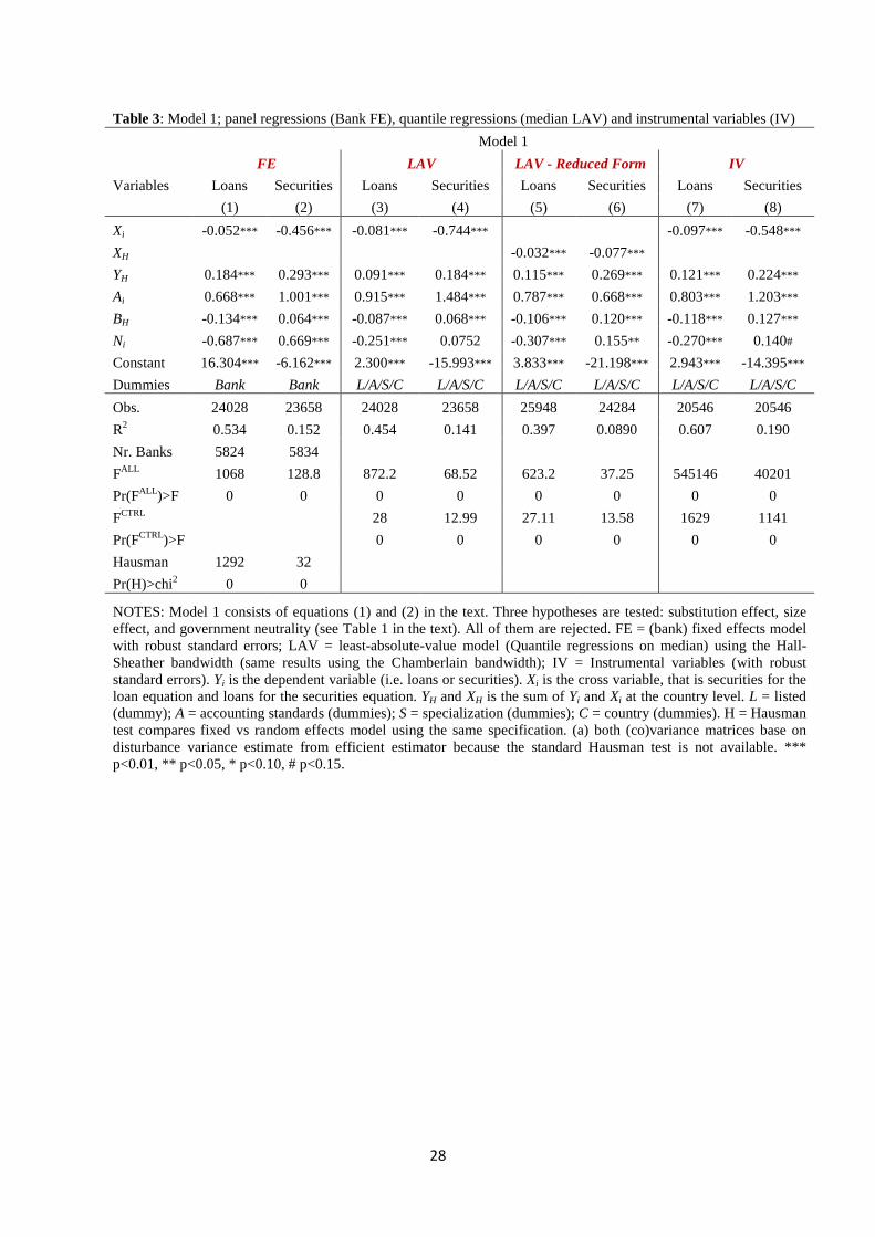
The results of Model 1, the benchmark model, are shown in Table 3. The first two

columns give the estimates of the panel regression with bank fixed effects (FE); the third and

fourth columns the estimates of the quantile regressions in the form of least-absolute-value

model (LAV); the fifth and sixth columns the LAV estimates for the two reduced-form

equations; and the last two columns the IV estimates of equations (1)-(2). We have data on

5.824 banks for loans and 5,834 for securities and the number of observations ranges from

20,546 to 25,948 depending on the estimation method. We ran both random and fixed effects

models but report only the latter based on the Hausman test; however, results are similar for

the two models. Fixed effects capture differences not only among banks, but also among

countries. R2 is consistently higher for Loans than for Securities, which could reflect in part

that total securities are a proxy of government securities.

As to the estimated coefficients, the elasticity of loans and securities to market

demand (YH) is positive and is consistent with a CAPM-type model. The relatively low

estimated value of beta is due to the incomplete universe of banks (six types) we have drawn

from Bankscope. Significantly negative coefficients for the cross-variable (Xi) indicate a

strong substitution effect between loans and securities; hence, H10 is rejected. The elasticties

relative to total assets (Ai) reject also the null hypothesis H20 that banks allocate Ai

proportionally between Li and Si: there is a preference for securities. The debt-to-GDP (BH)

coefficient is negative on loans and positive on securities, rejecting hypothesis H30 that banks

are neutral with respect to government debt in favor of the alternative of a mutual protection

pact between regulator and regulated banks. The coefficients of the ratio of non-performing

loans to total assets (Ni) mimic those of debt and reinforce the general pattern that the de-

18

risking is achieved by substituting securities for loans. A credit squeeze on the private sector

is the natural consequence of a financial crisis.

The next two columns of Table 3 show the estimates of the quantile regressions

(LAV) that treat the problem of potential outliers.16 In this case, we could not use the far too

numerous bank dummies, and replaced them with an assortment of dummies that tried to

capture bank characteristics such as whether they were listed, their type of accounting

standards, their type of specialization, as well as country dummies. All of these dummies are

jointly and highly significant statistically. LAV regressions confirm the signs and economic

impact of the FE regression coefficients, with two exceptions: the substitution effects are

stronger and the non-performing loans ratio does not impact securities.

In the next two columns of the table we show the estimates of the reduced-form

equations of Li and Si. In addition to the exogenous variables appearing on the right-hand side

of (5) and (6), we have added the four dummies that capture the bank characteristics noted in

the previous paragraph. The cross demand variable—SH in (5) and LH in (6)—has a negative

sign and is confirmed by the coefficient estimates of XH. A one percent increase in the

demand for loans raises Li by 0.115 percent and lowers Si by 0.077 percent, whereas a one

percent increase in the demand for securities raises Si by 0.269 percent and lowers Li by 0.032

percent; hence, an equal one percent increase in the demand for loans and securities shifts

banks’ portfolio toward securities by 0.11 percent. On the other hand, an increase in total

assets produces a slightly stronger response in Li than in Si, in contrast to the FE estimates.

In the final two columns of the table, we present the IV regressions to correct for the

endogeneity of Li and Si in systems (1)-(2) or (3)-(4). The instruments of IV include the

exogenous variables of the reduced-form equations plus the growth rate of deposits, the ratio

of liquid assets to total assets, the return on assets and the four bank-characteristic dummies;

16 The presence of outliers could bias standard econometric approaches, particularly when there are, as in our case, many missing and misreported values.

19

as such, the specification is in line with what we have done with FE and LAV. The difference

between IV and FE, in addition to the endogeneity treatment, consists in the four bank-

characteristic dummies and country dummies in place of bank fixed effects. There is a strong

similarity in the findings. In particular, there is confirmation that the substitution of securities

for loans is approximately five times as strong as the substitution of loans for securities. This

substitution pattern is reinforced by the stronger response of Si to Ai relative to the response

of Li to Ai. Finally, the biggest impact on asset reallocation originate from debt to GDP. By

multiplying the coefficient by the average value of BH, we obtain that over the entire period

BH has reduced loans by 9.07 percentage points and raised securities by 9.76 percentage

points, for a net reallocation effect towards securities of approximately 19 percentage points.

[Insert Table 3 here]

Table 4 shows the estimates of Model 2, which adds to the basic specification of

Table 3 the interaction of the debt-to-GDP ratio with YH and Ai, as well as the non-linearity in

BH. The interaction terms capture whether banks let variables of direct interest to the

regulator react to the evolution of BH. As we have done for previous hypotheses, we test that

banks are insensitive to the regulator’s concern (γ�=φ

�= 0 and λ� = µ

�= 0) against the

alternative that they are sensitive. The structure of Table 4 is similar to that of Table 3;

estimates and test statistics are, on the whole, also similar. The important finding is that the

interactive terms with BH are marginally significant: their impact is negative on loans in FE

and LAV, positive on securities in LAV and IV, and insignificant in the reduced form

equations. Thus, the null of H4 is “weakly” rejected against the alternative that the existence

of government debt raises the reaction of securities to market demand while lowering the

reaction of loans; in essence, there is some evidence that the debt-to-GDP ratio tilts the

allocation process towards securities, not only directly, but also indirectly through market

demand and total assets growth. The other relevant results of Table 4 is that the statistically

20

significant coefficient of B2H suggests the presence of threshold effects already emphasized in

the literature; see, for example, Minea and Parent (2012), Checherita-Westphal and Rother

(2012) and Law and Singh (2014). The novel aspect here is that the curvature for loans is

different than that of securities (concave).

[Insert Table 4 here]

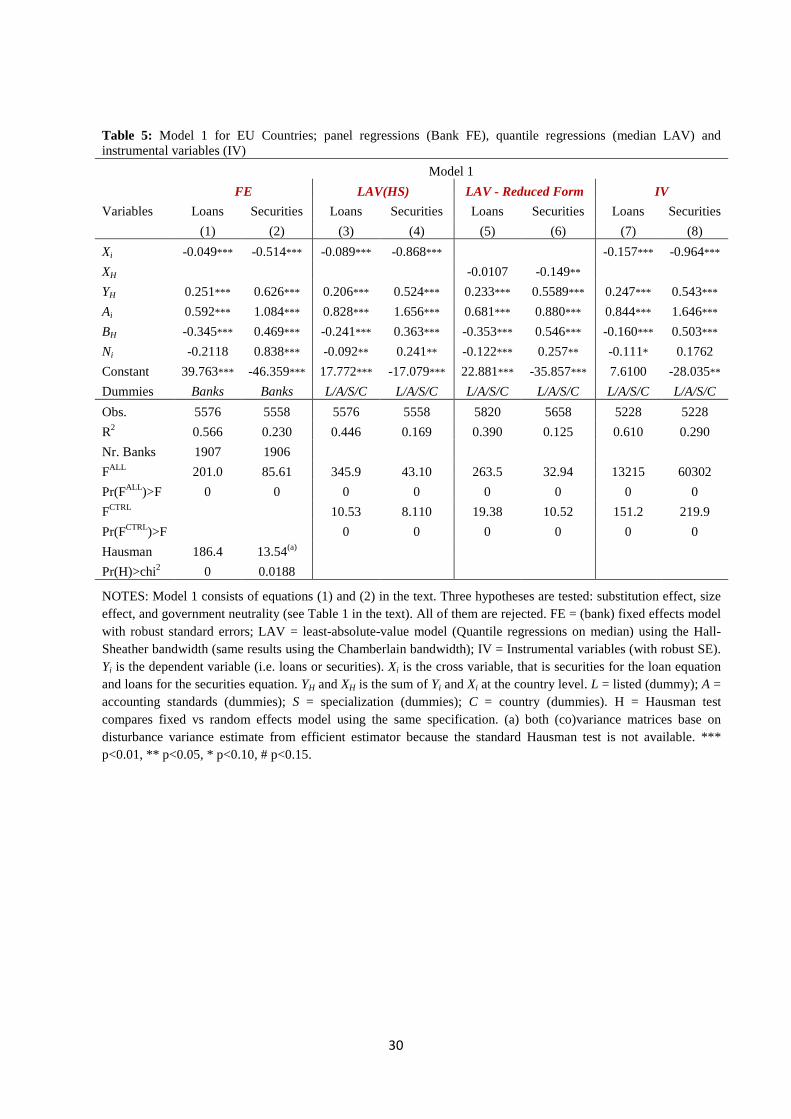
In the section on descriptive statistics we have shown that EU banks, largely in response

to the sovereign debt crisis, appear to have accentuated their portfolio re-adjustment towards

securities at the expense of credit to the private sector; and this pattern is particularly evident

for banks in the Southern EU countries.17 Therefore, we would expect the EU-area sample

estimates to differ from the world sample estimates in two significant ways: first, that

aggregate demand in the EU area would provide a further bias towards Si, and second that the

debt-to-GDP ratio would have larger absolute impacts on Si and Li. Table 5 confirms such

prediction. An equal one percentage point increase in YH in the two equations produces a

larger shift towards securities in the EU estimates than in the world estimates. A similar

finding holds for the debt-to-GDP. In sum, the security-bias in the portfolio reallocation for

the entire sample is accentuated in the EU area.

[Insert Table 5 here]

V. ROBUSTNESS

To check the robustness of our results, we run four econometric exercises. The first is to

measure the growth rate of market demand for loans and securities excluding bank i, that is

the observation of the bank on the left-hand side of the regression, in sympathy with what is

done in the industrial economics literature. The objective of this exercise is to check the

market power, or potential bias, of a large bank in the computation of the aggregate demand

variable. In a one-bank system, the left-hand side variable would be equal to YH; in a banking

17 See the relative movements of gross loans and securities in Figure 2.

21

system with a large number of equal-size banks, the left-hand side variable would have a

negligible impact on the computation of YH; in the more realistic case of a banking system

with a small number of big banks and a large number of small banks, the left-hand side

variable would be quite sensitive to the inclusion of a large bank in the computation of YH.

The first four columns of Table 6 (which shows for brevity only the benchmark FE and LAV

estimates) use the narrow definition of market demand, YH-1, instead of the broad definition,

YH. The YH-1 coefficients remain positive, although smaller in size and, in some cases, with

lesser statistical significance than those of YH in Table 3. In sum, this exercise, not

surprisingly, confirms that most banking systems display some degree of market power; yet,

our previous results hold.

The second exercise adds common and specific variables to the loans and securities

equations to further reduce the risk of relevant omitted variables. In Table 6 it is labelled as

Model 3: it extends the benchmark model of Table 3 with specific controls for loans and

securities. These controls are the equity-to-total assets ratio, Ei, the loans-to-deposits

coverage ratio, Ci, the growth rate of deposits, Di, the ratio of liquid assets to total assets Qi,

and the average return on assets, Ri. Our rationale for choosing Ei is that banks strive for an

optimal financial structure and, consequently, Li and Si could be sensitive to the evolution of

the current value of Ei in relation to an optimal but unobserved value. Ei is present in both

equations. Ci and Di are specific to the loan equations. Their justification are straightforward.

Since deposits are a more stable source of funding than alternative liabilities, banks may seek

to match deposits to long-term and unmarketable loans to reduce risk. Furthermore, a

predictable growth of deposits would further reduce uncertainty given the very short-term

maturity of deposits. Qi and Ri are instead specific to the security equation. While liquidity in

principle is a substitute for both loans and securities, we assume that the second substitution

dominates the first, particularly during a credit crunch. Ri is a broad measure of performance

22

with a potential ambiguous effect on Si. When loans’ credit risk is perceived to be high

relative to securities’, we would expect that a rising Ri would induce banks to favor securities

in their allocation strategy. When credit risk is perceived to be high equally for both loans

and securities, a rising Ri would induce banks to privilege liquidity and Si would decline.

The explanatory power of Model 3 with the five controls just discussed rises relative

to Model 2 estimates; see last four columns of Table 6. All the control variables are

statistically significant, except for Ei and Ri in the LAV securities equation. Ci and Di impact

the loan equation positively, as expected. Qi and Ri impact securities negatively and their sign

pattern is consistent with the well-publicized rush for liquidity. Our main results remain

unchanged.

[Insert Table 6 here]

The third exercise was to broaden the number of exogenous variables included in the

second step of the IV regressions of Table 3. The added controls are of two types, macro and

micro. The macro control consists of the country’s economic growth (real GDP). The micro

controls are the ratio of bank’s total business to total assets, the number of banks under the

same business group and the banks’ net interest margin. The four controls are first entered

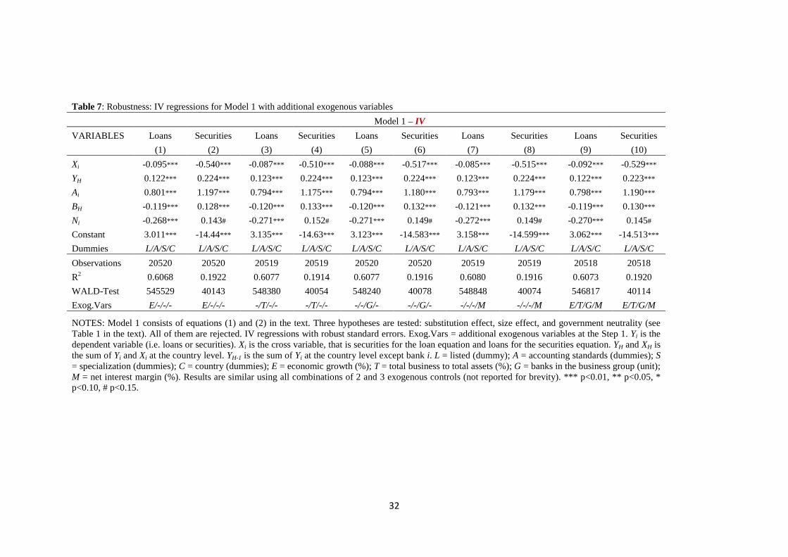
one at a time and then as a group in Table 7.18 There is a considerable degree of stability in

the sign, size, statistical and economic significance of the estimated coefficients and in the

explanatory power of the regressions across the table’s columns, a reflection that the

specification of the IV estimation of Table 3 remains robust to the four added macro and

micro controls.

[Insert Table 7 here]

The fourth and final step was to test the IV regression of Table 3 for the crisis period

2009-2012. We do not report the actual estimates here to save space but discuss the salient

18 We experimented with combinations of two and three controls with similar results. We don’t report results for brevity.

23

findings. The only material change in the loans equation in the crisis period affects the debt-

to-GDP ratio whose value drops to approximately one half of the coefficient’s value for the

entire period; the statistical significance remains the same, however. The material changes in

the securities equation occur in the substitution effect and in the response to aggregate

demand. The former goes from -0.548*** to -0.278*; the latter from .224* to .547***. The

implication is that during the crisis period banks have raised their allocation share in favor of

securities to changes in aggregate demand, while lowering their securities sensitivity to the

growth of loans. These patterns are what we would have expected and are in sympathy with

one of the main results of our study: a deep financial crisis penalizes credit to the private

sector.

VI CONCLUSIONS

This paper has examined how banks around the world have resized and reallocated their

earning assets in response to the subprime and sovereign debt crises. We have focused

especially on the interaction between sovereign debt and the bank asset allocation process.

After the crisis we observe a general substitution away from loans and in favor of securities,

substitution that was accompanied by a de-leveraging process at the world level and in the

Northern European countries, but not in the Southern European countries. The latter were

boosting their holdings of government debt at the expense of a significant reduction of credit

to the private sector. Our econometric findings corroborate that banks have readjusted the

composition of their assets and the overall regulatory credit risk by substituting securities for

loans. Banks, furthermore, have also been sensitive to those variables that are of direct

interest to the regulator.

The picture that emerges is a mutual protection pact regime, in which high-debt

governments exert pressure on banks, through the formal and informal regulatory system, to

24

privilege the purchase of government securities over credit to the private sector in exchange

for receiving protection against default. The quality of our findings is strengthened by the

large dataset we have used. While previous studies have focused on specific institutions,

typically large banks, ours encompasses the universe of the available categories of banks; and

to our knowledge, this is the first paper to do so.

As to specific hypotheses, we found strong substitution effects between loans and

securities, with the substitution of securities for loans being approximately five times as

strong as the substitution of loans for securities. This asymmetric pattern is reinforced by a

larger elasticity of securities with respect to total assets than the corresponding loan elasticity.

The debt-to-GDP coefficient has a negative impact on loans and positive on securities,

rejecting the hypothesis that banks are neutral with respect to government debt in favor of the

alternative of a “mutual protection pact” between regulator and regulated banks. The

evolution of the debt-to-GDP ratio has the biggest impact on asset re-allocation. European

Union banks have accentuated their portfolio readjustment towards securities at the expense

of credit to the private sector. Finally, during the crisis period 2009-2012, banks have further

raised their relative allocation share in favor of securities in response to changes in aggregate

demand, while lowering their securities sensitivity to the growth of loans. These patterns are

what we would have expected and are in sympathy with one of the main results of our study:

a deep financial crisis penalizes credit to the private sector

Our evidence that banks have effected de-risking by substituting securities for loans

reflects the Basel rule that government securities, a significant component of total securities,

have been accorded the special status of having a zero weight in the computation of risk-

weighted assets. The noted substitution lowers regulatory risk but not necessarily true

economic risk. The obvious policy recommendation would be to align regulatory risk to

economic risk, so as to achieve portfolio allocations based on return-risk profiles without the

25

murky considerations of moral hazard and mutual protection pacts. On the other hand, strict

public-choice analysis suggests that such a change is not likely to occur.

As to plans for future research on the subject, we have two extensions in mind. The

first is to focus on Eurozone banks and especially on the asymmetry between Northern and

Southern regions with a longer and updated period. We expect that financially stressed

Southern banks might have adopted more de-risking than de-leveraging to achieve relevant

risk reductions, whereas the opposite might have occurred in Northern banks. The second is

to examine in further detail how regulators impact on the asset allocation of bank portfolios

through the use of risk-weighted assets instead of market measures.

References

Acharya, V.V., Steffen, S. (2013), The “greatest” carry trade ever? Understanding Eurozone bank risks, NBER, WP 19039.

Acharya, V.V., Drechsler, I., Schnabl, P. (2014), A Pyrrhic Victory? Bank Bailouts and Sovereign Credit Risk, Journal of Finance (forthcoming), DOI: 10.1111/jofi.12206

Adelino, M., Ferreira, M.A. (2014), Bank Ratings and Lending Supply: Evidence from Sovereign Downgrades, available at SSRN: http://ssrn.com/abstract=2376721

Adrian, T., Shin, H.S. (2008), Liquidity and leverage, Federal Reserve Bank of New York, available online at http://www.newyorkfed.org/research/staff_reports/sr328.html.

Alessandrini, P., Fratianni, M., Hughes Hallett, A., Presbitero, A. (2014), External imbalances and fiscal fragility in the Euro area, Open Economies Review, 25: 3-34.

Angelini, P., Grande, G., Panetta, F. (2014), The negative feedback loop between banks and sovereigns, Banca d’Italia, WP 213, January 2014

Battistini, N., Pagano, M., Simonelli, S. (2013), Systemic risk and home bias in the Euro area, European Economy Working paper, February 6.

Bertrand M., Mehta P., Mullainathan S. (2002), Ferreting out tunnelling: an application to Indian business groups, Quarterly Journal of Economics, 117(1):121-148

Billor, N., Hadi, A.S., Velleman, P.F. (2000), BACON: Blocked adaptive computationally efficient outlier nominators, Computational Statistics & Data Analysis, 34: 279-29.

Broner, F., Erce, A., Martin, A., Ventura, J. (2013), Sovereign debt markets in turbulent times: Creditor discrimination and crowding-out effects, NBER Working Paper No. 19676.

26

Buch, C.M., Carstensen, K., Schertler, A. (2010), Macroeconomic Shocks and Banks’ Foreign Assets, Journal of Money, Credit and Banking, 42(1):171-188

Checherita-Westphal, C., Rother, P (2012). The impact of high government debt on economic growth and its channels: An empirical investigation for the euro area, European Economic Review, 56(7):1392–1405.

Fratianni, M., Marchionne, F. (2013), The fading stock market response to announcements of bank bailouts, Journal of Financial Stability, 9: 69-89.

Gomez Mejia, L., Haynes, K.T., Nunez, M., Jacobson, K., Moyano, J. (2007), Socio-emotional wealth and business risk in family-controlled firms: evidence from Spanish olive market. Administrative Science Quarterly. Q. 52, 106–137.

Hyun, J.S., Rhee, B.K. (2011), Bank capital regulation and credit supply, Journal of Banking & Finance, 35:323–330.

Hryckiewicz, A. (2014), What do we know about the impact of government interventions in the banking sector. An assessment of various bailout programs on bank behavior, Journal of International Financial Markets, Institutions and Money, 32:150–166

Kollmann, R. (2013), Global Banks, Financial Shocks, and International Business Cycles: Evidence from an Estimated Model, Journal of Money, Credit and Banking, 45(2):159-195

International Monetary Fund (online),World Economic Outlook Database; available at http://www.imf.org/external/pubs/ft/weo/2014/01/weodata/index.aspx

International Monetary Fund (2008), Global financial stability report: Financial stress and deleveraging, macrofinancial implications and policy, October 2008, Washington, DC.

Law, S.H., Singh, N. (2014), Does too much finance harm economic growth? Journal of Banking & Finance, 41 (2014) 36–44

Levy, H., Levy, M. (2014), The home bias is here to stay, Journal of Banking & Finance, 47:29-40

Merler, S., Pisani-Ferry, J. (2012), Sudden stops in the euro area, Review of Economics and Institutions, 3(3):Article 5.

Minea, A., Parent, A. (2012), Is high public debt always harmful to economic growth? Reinhart and Rogoff and some complex nonlinearities, Association Francaise de Cliometrie, WP 8.

Popov, A., van Horen, N. (2013). The impact of sovereign debt exposure on bank lending. Evidence from the European debt crisis, De Nederlandsche Bank Working Paper, No. 382

Rousseeuw, P.J., van Zomeren, B. (1990), Unmasking multivariate outliers and leverage points (with discussion), Journal of the American Statistical Association, 85:633-639.

Rousseeuw, P.J., van Driessen, K. (1999), A fast algorithm for the minimum covariance determinant estimator, Technometrics, 41:212-223.

Sraer D., Thesmar D. (2007), Performance and Behaviour of Family Firms: Evidence from the French Stock Market, Journal of the European Economic Association, 5(4):709–751

27

Table 1: Summary of hypotheses testing

HYP Name H0 Ha

1 Substitution effect −�� = −β�= 0 −�� < 0, −β

�< 0

2 Size effect �� = β�= 1 �� < β

�

3 Neutrality of the government −�� = −β�= 0 −�� < 0, −β

�> 0

4 Demand sensitivity to regulator γ�=φ

�= 0 γ

�,φ

�≠ 0

NOTES: HYP = hypothesis number, H0 = null hypothesis, Ha = alternative hypothesis. Coefficients refer to equations (1)-(4).

Table 2: Descriptive statistics on cleaned Bankscope data

Variables Mean St.Dev Min Median Max Nr.Obs. Skew. Kurt. PANEL A: Bank-level variables

Gross Loans (th USD) 889380 1351278 0.27 324127 7280833 54331 2.44 8.89

Total Securities (th USD) 311159 507139 0.03 91692 2631347 52720 2.43 8.69

Total Assets (th USD) 1691330 2631584 38.65 565254 13900000 55350 2.46 8.94

Total Equity (th USD) 137490 208641 7.7 49005 1093173 55491 2.43 8.78

Total Deposits (th USD) 963834 1435918 0.03 346714 7397910 52778 2.30 8.07

Impaired Loans (th USD) 40026 65885 0.07 9947 339115 32757 2.35 8.30

Liquid Assets (th USD) 223604 358711 1 63600 1893717 55121 2.42 8.70

Coverage Ratio (%) 97.50 50.70188 0.01 87.60 311.56 52693 1.34 5.59

Return on Assets (%) 0.62 0.82 -2.63 0.43 3.98 58690 0.65 6.09

Listed (dummy) 0.07 0.25 0 0 1 160963 3.41 12.62

Accounting

IFRS (dummy) 0.08 0.27 0 0 1 160963 3.05 10.30

Regulatory (dummy) 0.43 0.50 0 0 1 160963 0.28 1.08

GAAP (dummy) 0.27 0.44 0 0 1 160963 1.02 2.05

Specialization

Holding (dummy) 0.14 0.34 0 0 1 160963 2.12 5.48

Commercial (dummy) 0.59 0.49 0 1 1 160963 -0.36 1.13

Cooperative (dummy) 0.12 0.33 0 0 1 160963 2.28 6.20

Investment (dummy) 0.02 0.15 0 0 1 160963 6.50 43.26

Real Estate (dummy) 0.01 0.12 0 0 1 160963 8.08 66.36

Saving (dummy) 0.11 0.32 0 0 1 160963 2.412 6.85

PANEL B: Country-level variables

Debt-to-GDP ratio (%) 56.61 37.65 3.68 47.50 238.02 344 1.67 7.58

NOTES: Period: 2005-2012. We use 2004 to compute growth rate (see other tables). Total observations: 160,963. Number of banks: 20,236.

28

Table 3: Model 1; panel regressions (Bank FE), quantile regressions (median LAV) and instrumental variables (IV)

Model 1

FE LAV LAV - Reduced Form IV

Variables Loans Securities Loans Securities Loans Securities Loans Securities

(1) (2) (3) (4) (5) (6) (7) (8)

Xi -0.052*** -0.456*** -0.081*** -0.744*** -0.097*** -0.548***

XH -0.032*** -0.077***

YH 0.184*** 0.293*** 0.091*** 0.184*** 0.115*** 0.269*** 0.121*** 0.224***

Ai 0.668*** 1.001*** 0.915*** 1.484*** 0.787*** 0.668*** 0.803*** 1.203***

BH -0.134*** 0.064*** -0.087*** 0.068*** -0.106*** 0.120*** -0.118*** 0.127***

Ni -0.687*** 0.669*** -0.251*** 0.0752 -0.307*** 0.155** -0.270*** 0.140#

Constant 16.304*** -6.162*** 2.300*** -15.993*** 3.833*** -21.198*** 2.943*** -14.395***

Dummies Bank Bank L/A/S/C L/A/S/C L/A/S/C L/A/S/C L/A/S/C L/A/S/C

Obs. 24028 23658 24028 23658 25948 24284 20546 20546

R2 0.534 0.152 0.454 0.141 0.397 0.0890 0.607 0.190

Nr. Banks 5824 5834

FALL 1068 128.8 872.2 68.52 623.2 37.25 545146 40201

Pr(FALL)>F 0 0 0 0 0 0 0 0

FCTRL 28 12.99 27.11 13.58 1629 1141

Pr(FCTRL)>F 0 0 0 0 0 0

Hausman 1292 32

Pr(H)>chi2 0 0

NOTES: Model 1 consists of equations (1) and (2) in the text. Three hypotheses are tested: substitution effect, size effect, and government neutrality (see Table 1 in the text). All of them are rejected. FE = (bank) fixed effects model with robust standard errors; LAV = least-absolute-value model (Quantile regressions on median) using the Hall-Sheather bandwidth (same results using the Chamberlain bandwidth); IV = Instrumental variables (with robust standard errors). Yi is the dependent variable (i.e. loans or securities). Xi is the cross variable, that is securities for the loan equation and loans for the securities equation. YH and XH is the sum of Yi and Xi at the country level. L = listed (dummy); A = accounting standards (dummies); S = specialization (dummies); C = country (dummies). H = Hausman test compares fixed vs random effects model using the same specification. (a) both (co)variance matrices base on disturbance variance estimate from efficient estimator because the standard Hausman test is not available. *** p<0.01, ** p<0.05, * p<0.10, # p<0.15.

29

Table 4: Model 2; panel regressions (Bank FE), quantile regressions (median LAV) and instrumental variables (IV)

Model 2

FE LAV(HS) LAV - Reduced Form IV

Variables Loans Securities Loans Securities Loans Securities Loans Securities

(1) (2) (3) (4) (5) (6) (7) (8)

Xi -0.055*** -0.482*** -0.080*** -0.735*** -0.103*** -0.517***

XH 0.080*** 0.098*

XBH -0.002*** -0.004***

YH 0.230*** 0.297*** 0.122*** 0.133*** 0.125*** 0.304*** 0.087*** -0.0240

YBH -0.001* 0.0006 -0.0004* 0.001* -0.0003 -0.0002 0.0004 0.004***

Ai 0.580*** 0.783*** 0.874*** 1.325*** 0.713*** 0.381*** 0.716*** 0.983***

ABi 0.002*** 0.004*** 0.0005*** 0.002*** 0.001*** 0.004*** 0.001*** 0.003***

BH -0.221*** 0.084** -0.162*** 0.151*** -0.215*** 0.265*** -0.205*** 0.238***

BH2 0.0003*** -0.00003 0.0003*** -0.0003*** 0.0004*** -0.0006*** 0.0004*** -0.0004***

Ni -0.600*** 0.626*** -0.201*** 0.0211 -0.229*** 0.144* -0.226*** 0.0975

Constant 19.808*** -7.949*** 3.247*** -15.410*** 4.701*** -20.284*** 5.381*** -11.171***

Dummies Bank Bank L/A/S/C L/A/S/C L/A/S/C L/A/S/C L/A/S/C L/A/S/C

Obs. 24028 23658 24028 23658 25948 24284 20546 20546

R2 0.540 0.161 0.456 0.143 0.401 0.0970 0.610 0.196

Nr. Banks 5824 5834

FALL 809.6 139.2 942.1 86.01 705.0 50.84 346540 97473

Pr(FALL)>F 0 0 0 0 0 0 0 0

FCTRL 26.76 11.63 27.18 12.43 1525 826.3

Pr(FCTRL)>F 0 0 0 0 0 0

Hausman 756.6 256.4

Pr(H)>chi2 0 0

NOTES: Model 2 consists of equations (3) and (4) in the text. Four hypotheses are tested: substitution effect, size effect, government neutrality, and demand sensitivity to regulator (see Table 1 in the text). The first three are strongly rejected, the fourth is weakly rejected. FE = (bank) fixed effects model with robust standard errors; LAV = least-absolute-value model (Quantile regressions on median) using the Hall-Sheather bandwidth (same results using the Chamberlain bandwidth); IV = Instrumental variables (with robust SE). Yi is the dependent variable (i.e. loans or securities). Xi is the cross variable, that is securities for the loan equation and loans for the securities equation.YH and XH is the sum of Yi and Xi at the country level. L = listed (dummy); A = accounting standards (dummies); S = specialization (dummies); C = country (dummies). H = Hausman test compares fixed vs random effects model using the same specification. (a) both (co)variance matrices base on disturbance variance estimate from efficient estimator because the standard Hausman test is not available. *** p<0.01, ** p<0.05, * p<0.10, # p<0.15.

30

Table 5: Model 1 for EU Countries; panel regressions (Bank FE), quantile regressions (median LAV) and instrumental variables (IV)

Model 1

FE LAV(HS) LAV - Reduced Form IV

Variables Loans Securities Loans Securities Loans Securities Loans Securities

(1) (2) (3) (4) (5) (6) (7) (8)

Xi -0.049*** -0.514*** -0.089*** -0.868*** -0.157*** -0.964***

XH -0.0107 -0.149**

YH 0.251*** 0.626*** 0.206*** 0.524*** 0.233*** 0.5589*** 0.247*** 0.543***

Ai 0.592*** 1.084*** 0.828*** 1.656*** 0.681*** 0.880*** 0.844*** 1.646***

BH -0.345*** 0.469*** -0.241*** 0.363*** -0.353*** 0.546*** -0.160*** 0.503***

Ni -0.2118 0.838*** -0.092** 0.241** -0.122*** 0.257** -0.111* 0.1762

Constant 39.763*** -46.359*** 17.772*** -17.079*** 22.881*** -35.857*** 7.6100 -28.035**

Dummies Banks Banks L/A/S/C L/A/S/C L/A/S/C L/A/S/C L/A/S/C L/A/S/C

Obs. 5576 5558 5576 5558 5820 5658 5228 5228

R2 0.566 0.230 0.446 0.169 0.390 0.125 0.610 0.290

Nr. Banks 1907 1906

FALL 201.0 85.61 345.9 43.10 263.5 32.94 13215 60302

Pr(FALL)>F 0 0 0 0 0 0 0 0

FCTRL 10.53 8.110 19.38 10.52 151.2 219.9

Pr(FCTRL)>F 0 0 0 0 0 0

Hausman 186.4 13.54(a)

Pr(H)>chi2 0 0.0188

NOTES: Model 1 consists of equations (1) and (2) in the text. Three hypotheses are tested: substitution effect, size effect, and government neutrality (see Table 1 in the text). All of them are rejected. FE = (bank) fixed effects model with robust standard errors; LAV = least-absolute-value model (Quantile regressions on median) using the Hall-Sheather bandwidth (same results using the Chamberlain bandwidth); IV = Instrumental variables (with robust SE). Yi is the dependent variable (i.e. loans or securities). Xi is the cross variable, that is securities for the loan equation and loans for the securities equation. YH and XH is the sum of Yi and Xi at the country level. L = listed (dummy); A = accounting standards (dummies); S = specialization (dummies); C = country (dummies). H = Hausman test compares fixed vs random effects model using the same specification. (a) both (co)variance matrices base on disturbance variance estimate from efficient estimator because the standard Hausman test is not available. *** p<0.01, ** p<0.05, * p<0.10, # p<0.15.

31

Table 6: Robustness; panel regressions (Bank FE) and quantile regression (median LAV) with YH and controls

Model 1 (with modified demand) Model 3 (additional controls)

FE FE LAV LAV FE FE LAV LAV

Variables Loans Securities Loans Securities Loans Securities Loans Securities

(1) (2) (1) (2) (3) (4) (3) (4)

Xi -0.050*** -0.393*** -0.081*** -0.713*** -0.055*** -0.655*** -0.085*** -0.844***

YH-1 0.030** 0.018** 0.008* 0.009***

YH 0.139*** 0.275*** 0.075*** 0.178***

Ai 0.677*** 0.950*** 0.930*** 1.452*** 0.759*** 1.251*** 0.936*** 1.591***

BH -0.142*** 0.095*** -0.091*** 0.076*** -0.098*** 0.092*** -0.082*** 0.081***

Ni -0.693*** 0.636*** -0.238*** 0.0561 -0.768*** 0.794*** -0.322*** 0.084

Ei 0.435*** 0.336* 0.083*** -0.032

Ci 0.250*** 0.047***

Qi -0.972*** -0.285***

Di 0.627*** 0.154***

Ri -1.426** -0.115

Constant 17.066*** -8.086*** 3.060*** -14.211*** -60.720*** 2.633 -15.157*** -8.062***

Dummies Banks Banks L/A/S/C L/A/S/C Banks Banks L/A/S/C L/A/S/C

Obs. 24777 24780 24777 24780 21613 22332 21613 22332

Nr of banks 5904 5905 5219 5590

R2 0.522 0.127 0.458 0.124 0.623 0.179 0.484 0.150

FALL 924.8 64.02 852.7 66.54 1016 78.20 930.1 72.90

Pr(FALL )>F 0 0 0 0 0 0 0 0

FCTRL 28.70 12.97 109.8 51.06 32.67 15.10

Pr(FCTRL)>F 0 0 0 0 0 0

H 238.2 54 376.7 360.9

Pr(H)>chi2 0 0 0 0

NOTES: Model 3 adds to Model 1 (equations (1) and (2) in the text) a set of controls with continuous common and specific bank variables. Three hypotheses are tested: substitution effect, size effect, and government neutrality (see Table 1 in the text). All of them are rejected. FE = bank fixed effects model with robust standard errors. LAV = least-absolute-value model (quantile regressions with median) using the Hall-Sheather bandwidth (same results using the Chamberlain bandwidth). Yi is the dependent variable (i.e. loans or securities). Xi is the cross variable, that is securities for the loan equation and loans for the securities equation. YH and XH is the sum of Yi and Xi at the country level. L = listed (dummy); A = accounting standards (dummies); S = specialization (dummies); C = country (dummies).H = Hausman test compares fixed vs random effects model using the same specification. *** p<0.01, ** p<0.05, * p<0.10, # p<0.15.

32

Table 7: Robustness: IV regressions for Model 1 with additional exogenous variables

Model 1 – IV

VARIABLES Loans Securities Loans Securities Loans Securities Loans Securities Loans Securities

(1) (2) (3) (4) (5) (6) (7) (8) (9) (10)

Xi -0.095*** -0.540*** -0.087*** -0.510*** -0.088*** -0.517*** -0.085*** -0.515*** -0.092*** -0.529***

YH 0.122*** 0.224*** 0.123*** 0.224*** 0.123*** 0.224*** 0.123*** 0.224*** 0.122*** 0.223***

Ai 0.801*** 1.197*** 0.794*** 1.175*** 0.794*** 1.180*** 0.793*** 1.179*** 0.798*** 1.190***

BH -0.119*** 0.128*** -0.120*** 0.133*** -0.120*** 0.132*** -0.121*** 0.132*** -0.119*** 0.130***

Ni -0.268*** 0.143# -0.271*** 0.152# -0.271*** 0.149# -0.272*** 0.149# -0.270*** 0.145#

Constant 3.011*** -14.44*** 3.135*** -14.63*** 3.123*** -14.583*** 3.158*** -14.599*** 3.062*** -14.513***

Dummies L/A/S/C L/A/S/C L/A/S/C L/A/S/C L/A/S/C L/A/S/C L/A/S/C L/A/S/C L/A/S/C L/A/S/C

Observations 20520 20520 20519 20519 20520 20520 20519 20519 20518 20518

R2 0.6068 0.1922 0.6077 0.1914 0.6077 0.1916 0.6080 0.1916 0.6073 0.1920

WALD-Test 545529 40143 548380 40054 548240 40078 548848 40074 546817 40114

Exog.Vars E/-/-/- E/-/-/- -/T/-/- -/T/-/- -/-/G/- -/-/G/- -/-/-/M -/-/-/M E/T/G/M E/T/G/M

NOTES: Model 1 consists of equations (1) and (2) in the text. Three hypotheses are tested: substitution effect, size effect, and government neutrality (see Table 1 in the text). All of them are rejected. IV regressions with robust standard errors. Exog.Vars = additional exogenous variables at the Step 1. Yi is the dependent variable (i.e. loans or securities). Xi is the cross variable, that is securities for the loan equation and loans for the securities equation. YH and XH is the sum of Yi and Xi at the country level. YH-1 is the sum of Yi at the country level except bank i. L = listed (dummy); A = accounting standards (dummies); S = specialization (dummies); C = country (dummies); E = economic growth (%); T = total business to total assets (%); G = banks in the business group (unit); M = net interest margin (%). Results are similar using all combinations of 2 and 3 exogenous controls (not reported for brevity). *** p<0.01, ** p<0.05, * p<0.10, # p<0.15.

33

Figure 1: Boxplot and frequency distribution after the cleaning procedures: growth rate of gross loans (%), total securities (%), and total assets (%).

NOTES: Our elaborations on Bankscope data.

34

Figure 2: De-leveraging and de-risking: World, Northern and Southern EU countries.

NOTES: Our elaboration on Bankscope data. WORLD = all sample countries, NEU = Northern European Union countries, SEU = Southern European Union countries.

35

DATA APPENDIX

Table A.1: Variable definition and sources.

Variable Description Source or Formula

Gross Loans Total amount of issued credits given to banks

during the accounting period (th. USD) Bankscope

Total Securities Total amount of securities in bank asset portfolio

(th. USD) Bankscope

Total Assets Total value of all bank current and long-term assets

(th. USD) Bankscope

Total Deposits The sum of interest and non-interest bearing deposit

accounts at a bank (th. USD) Bankscope

Total Equity The total amount of common and preferred

stock equity of the bank (th. USD) Bankscope

Liquid Assets Cash and central bank reserves of the bank (th.

USD) Bankscope

Impaired Loans The amount for which it is not likely the bank will

collect the full value of the loans because the borrowers’ creditworthiness is fallen (th. USD)

Bankscope

Li Growth rate in percentage of Gross Loans at the

(individual) bank level (%) �3 =

GrossLoans3,?

GrossLoans3,?)�− 1

LH Growth rate in percentage of Gross Loans at the

(market) country level (%) �@ =

∑ GrossLoans3,?�∈�

∑ GrossLoans3,?)��∈�

− 1

Si Growth rate in percentage of Total Securities at the

(individual) bank level (%) �3 =

TotalSecurities3,?

TotalSecurities3,?)�− 1

SH Growth rate in percentage of Total Securities at the

(market) country level (%) �@ =

∑ TotalSecurities3,?�∈�

∑ TotalSecurities3,?)��∈�

− 1

Ai Growth rate in percentage of Total Assets at the

(individual) bank level (%) �3 =

TotalAssets3,?

TotalAssets3,?)�− 1

Ni Ratio of Non-Performing Loans to Total Assets (%) �3 =ImpairedLoans3,?

TotalAssets3,?

BH Debt-to-GDP ratio (%) World Economic Outlook

Ei Ratio of Total Equity to Total Assets (%) /3 =TotalEquity3,?

TotalAssets3,?

Ci Loans-to-deposit coverage ratio (%) �3 =ImpairedLoans3,?

TotalAssets3,?

Di Growth rate of Total Deposits (%) S3 =TotalDeposits3,?

TotalDeposits3,?)�− 1

Qi Ratio of Liquid Assets to Total Assets (%) �3 =LiquidAssets3,?

TotalAssets3,?

Ri Return on Average (Total) Assets (%) Bankscope E Real economic growth rate (%) World Economic Outlook B Ratio of total business to total assets (%) Bankscope

G Number of banks in the business group (unit) Bankscope M Net interest margin at the bank level (%) Bankscope

36

Table A.2: Treatment of outliers on the downloaded variables in level.

Variables Bankscope BACON NEG IQR Final

Gross Loans

Obs 81695 80530 79829 70186 54331 Min -3420.15 -3420.15 0.1 0.1 0.27 Max 3070086000 3070086000 3070086000 7280833 7280833 Mean 10156189.38 6136621.19 6190508.56 910514.92 889380.41

Total Securities

Obs 80368 79203 76779 67389 52720 Min -13565.13 -13565.13 0.03 0.03 0.03 Max 3195801331 3195801331 3195801331 2631346.97 2631346.97 Mean 7990021.14 4472523.65 4613726.74 309709.2 311158.64

Total Assets

Obs 82579 81414 81414 71754 55350 Min 14.29 14.29 14.29 14.29 38.65 Max 4682924032 4682924032 4682924032 13882655 13882655 Mean 22394247.56 13386591.24 13386591.24 1751408.03 1691330.07

Impaired Loans

Obs 48937 47772 46498 41138 32757 Min -18242.98 -18242.98 0.04 0.04 0.07 Max 251949000 251949000 251949000 339114.89 339114.89 Mean 515310.57 265718.63 272999.46 39960.35 40025.82

Total Equity

Obs 82574 81409 81078 71882 55491 Min -136279008 -136279008 0.55 0.55 7.7 Max 923629888 923629888 923629888 1093172.88 1093172.88 Mean 1285075.58 817295.21 840265.08 144538.01 137490.11

Liquid Assets

Obs 82322 81157 81033 71424 55121 Min -1803.25 -1803.25 0.04 0.04 1 Max 1416300800 1416300800 1416300800 1893717.25 1893717.25 Mean 4979323.99 2787035.15 2791300.03 227780.23 223603.8

Total Deposits

Obs 76554 75389 74568 66171 52778 Min 0 0 0.03 0.03 0.03 Max 3399283200 3399283200 3399283200 7397909.5 7397909.5 Mean 10156573.62 5614214.58 5676027.56 958397.52 963833.92

Return on Assets

Obs 82099 80934 80934 75615 58690 Min -348.07 -348.07 -348.07 -2.63 -2.63 Max 257.21 257.21 257.21 3.98 3.98 Mean 0.81 0.82 0.82 0.66 0.62

Total Obs 219690 218525 218525 218525 160963 Banks 21969 21968 21968 21968 20236

NOTES: BACON = blocked adaptive computationally efficient outlier nominators (BACON) algorithm to identify multivariate outliers proposed by Billor, Hadi, and Velleman (2000). A flagged outlier reveals a systematic errors and the whole record is cancelled. NEG = negative values for non-negative defined accounting items. A flagged outlier reveals an idiosyncratic error and its entry is replaced with a missing value. IQR = outliers identification method based on the interquartile range IQ. A point beyond an outer fence is considered an extreme outlier. The lower outer fence is �1 − 3 ∗ "� where Q1=lower quartile. The higher outer fence is �3 + 3 ∗ "� where Q3=upper quartile. Extreme outliers are considered idiosyncratic errors and replaced with missing values. In “Final”, we select 6 kinds of banks: bank holdings and holding companies, commercial banks, cooperative banks, investment banks, real estate and mortgage banks, and savings banks.

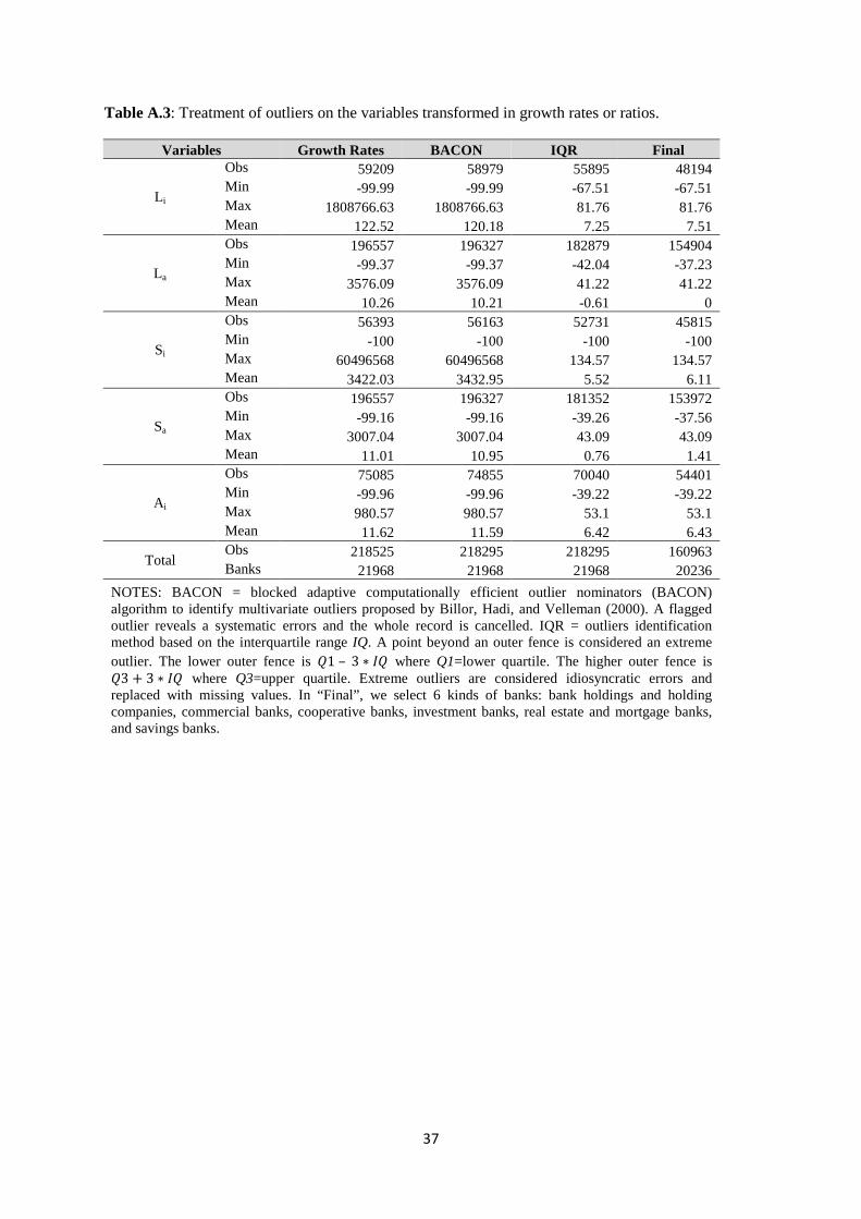
37

Table A.3: Treatment of outliers on the variables transformed in growth rates or ratios.

Variables Growth Rates BACON IQR Final

L i

Obs 59209 58979 55895 48194 Min -99.99 -99.99 -67.51 -67.51 Max 1808766.63 1808766.63 81.76 81.76 Mean 122.52 120.18 7.25 7.51

La

Obs 196557 196327 182879 154904 Min -99.37 -99.37 -42.04 -37.23 Max 3576.09 3576.09 41.22 41.22 Mean 10.26 10.21 -0.61 0

Si

Obs 56393 56163 52731 45815 Min -100 -100 -100 -100 Max 60496568 60496568 134.57 134.57 Mean 3422.03 3432.95 5.52 6.11

Sa

Obs 196557 196327 181352 153972 Min -99.16 -99.16 -39.26 -37.56 Max 3007.04 3007.04 43.09 43.09 Mean 11.01 10.95 0.76 1.41

A i

Obs 75085 74855 70040 54401 Min -99.96 -99.96 -39.22 -39.22 Max 980.57 980.57 53.1 53.1 Mean 11.62 11.59 6.42 6.43

Total Obs 218525 218295 218295 160963 Banks 21968 21968 21968 20236

NOTES: BACON = blocked adaptive computationally efficient outlier nominators (BACON) algorithm to identify multivariate outliers proposed by Billor, Hadi, and Velleman (2000). A flagged outlier reveals a systematic errors and the whole record is cancelled. IQR = outliers identification method based on the interquartile range IQ. A point beyond an outer fence is considered an extreme outlier. The lower outer fence is �1– 3 ∗ "� where Q1=lower quartile. The higher outer fence is �3 + 3 ∗ "� where Q3=upper quartile. Extreme outliers are considered idiosyncratic errors and replaced with missing values. In “Final”, we select 6 kinds of banks: bank holdings and holding companies, commercial banks, cooperative banks, investment banks, real estate and mortgage banks, and savings banks.

38

Figure A.1: Boxplot on final data and original data downloaded from Bankscope

NOTES: The order of magnitude of the x-axis scale on the left (Final Data) is 3 digits smaller than that on the right (Bankscope Data). There is a trade-off between data cleaning and the number of observations. The boxplots on Final Data suggest that the outlier problems could be not completely removed. Stricter cleaning criteria would have reduced excessively the number of observations.