bandwidth measurements in wired and wireless networks - idt - mrtc

Malardalen University Licentiate ThesisNo.48

Bandwidth Measurements inWired and Wireless Networks

Andreas Johnsson

April 2005

Department of Computer Science and ElectronicsMalardalen University

Vasteras, Sweden

Copyright c Andreas Johnsson, 2005ISSN 1651-9256ISBN 91-88834-53-0Printed by Arkitektkopia, Vasteras, SwedenDistribution: Malardalen University Press

Abstract

In the Internet today, end-user applications cannot get bandwidth guaranteesfrom the network. Instead, bandwidth measures, such as available bandwidthand link capacity, must be measured whereafter the application can adapt itssend rate to the bandwidth measurement estimate. An exampleapplicationthat rely on bandwidth measurements is TV transmission in realtime over theInternet.

To measure the available bandwidth between two nodes in a computer net-work, such as the Internet, active measurement methods are used. These meth-ods do not require prior knowledge about the network topology. Measurementdata, divided intoprobe packets, is injected into the network with an initialpacket separation. The packets are time stamped on the receiver side. Bydeploying analysis methods the available bandwidth and link capacity can becalculated using the initial separation and the time stampsas input.

The work presented in this licentiate thesis studies bandwidth measurementmethods with two foci: a)how can the interactions between probe packets andother traffic in the network be described?and b)how do existing measurementmethods, designed for wired networks, behave in wireless networks?

A framework has been developed to describe the interactionsbetween probepackets and other network traffic packets. This framework also describes thedifferences between using the statistical mean and median operator on timestamps in an analysis.

A simplified version of the TOPP measurement method, called DietTopp,has been developed and implemented. DietTopp is evaluated and compared toother bandwidth measurement tools in both wired and wireless scenarios.

Results obtained from measurements in wireless 802.11b networks showimportant differences compared to measurement results obtained from wirednetworks. The origins to some of the observed differences are explained whereassome are left to future research.

i

To my family

Acknowledgements

First of all I would like to thank my two supervisors and friends, Mats Bjorkmanand Bob Melander. Without your guidance, creative support and collaborationI never would have made it this far. I hope that you both will have the time andpatience to continue the journey towards a doctoral degree with me.

I would like to thank Svante Ekelin, Annikki Welin and RikardHolm atEricsson Research for creative discussions and for helpingme with many ofthe measurements presented in this thesis.

To Svante Ekelin, Jan-Erik Mangs, at Ericsson Research, Erik Hartikainenat Linkoping University, Martin Nilsson at SICS and my supervisors MatsBjorkman and Bob Melander: I hope our ongoing collaboration will resultin fruitful research!

Furthermore I would like to thank Jonas Neander and Ewa Hansen, bothpart of the data communication group at Malardalen University, for their sup-port as fellow Ph.D. students.

I also want to send my great thanks to the rest of the personal at our depart-ment for interesting discussions, coffee break laughs and in general for makingour department a creative and fun place.

I wish to thank the present and old CoRe-group members at Uppsala Uni-versity for letting me visit their department once a week andfor many fun andinteresting discussions. Input and feedback from Christian Rohner and HenrikLundgren have been rewarding, thank you.

I would like to thank my family who has always supported me anden-couraged me to strive towards becoming a researcher. I also want to thank myfriends for enriching my spare time. Finally, to my girlfriend Maaret, thankyou for keeping me motivated in my studies and especially formaking my lifeoutside work full of joy. I love you.

v

vi

Many great thanks to our generous sponsors: the Swedish Research Coun-cil, Vinnova and the KK Foundation. Financial support for travels, other visitsand courses has also been granted from ARTES++.

Andreas JohnssonVasteras, April 2005

Contents

List of Publications 1

I Thesis 3

1 Introduction 51.1 Background and motivation . . . . . . . . . . . . . . . . . . . 51.2 IP networks . . . . . . . . . . . . . . . . . . . . . . . . . . . 71.3 Research area . . . . . . . . . . . . . . . . . . . . . . . . . . 10

1.3.1 Network measurements . . . . . . . . . . . . . . . . . 101.3.2 Link capacity and available bandwidth . . . . . . . . . 131.3.3 Problems . . . . . . . . . . . . . . . . . . . . . . . . 151.3.4 Testing and verification . . . . . . . . . . . . . . . . . 16

1.4 Our research . . . . . . . . . . . . . . . . . . . . . . . . . . . 171.4.1 Research problems . . . . . . . . . . . . . . . . . . . 171.4.2 Research method . . . . . . . . . . . . . . . . . . . . 191.4.3 Contributions . . . . . . . . . . . . . . . . . . . . . . 20

2 Related work 212.1 Introduction . . . . . . . . . . . . . . . . . . . . . . . . . . . 212.2 Bandwidth measurement tools . . . . . . . . . . . . . . . . . 22

2.2.1 Packet rate methods . . . . . . . . . . . . . . . . . . 222.2.2 Packet gap methods . . . . . . . . . . . . . . . . . . . 242.2.3 Link capacity estimation . . . . . . . . . . . . . . . . 25

2.3 Measurements in wireless networks . . . . . . . . . . . . . . 262.4 Applications of bandwidth measurements . . . . . . . . . . . 26

vii

viii Contents

3 Summary of papers 293.1 Paper A . . . . . . . . . . . . . . . . . . . . . . . . . . . . . 293.2 Paper B . . . . . . . . . . . . . . . . . . . . . . . . . . . . . 303.3 Paper C . . . . . . . . . . . . . . . . . . . . . . . . . . . . . 303.4 Paper D . . . . . . . . . . . . . . . . . . . . . . . . . . . . . 31

4 Conclusions and future work 33

Bibliography 35

II Included Papers 39

5 Paper A:On the Analysis of Packet-Train Probing Schemes 415.1 Introduction . . . . . . . . . . . . . . . . . . . . . . . . . . . 435.2 Description of patterns . . . . . . . . . . . . . . . . . . . . . 44

5.2.1 A multiple-hop model for route delay variation . . . . 445.2.2 Mirror pattern . . . . . . . . . . . . . . . . . . . . . . 465.2.3 Chain pattern . . . . . . . . . . . . . . . . . . . . . . 485.2.4 Quantification pattern . . . . . . . . . . . . . . . . . . 49

5.3 Testbed setup . . . . . . . . . . . . . . . . . . . . . . . . . . 515.4 Signatures . . . . . . . . . . . . . . . . . . . . . . . . . . . . 52

5.4.1 The independence signature . . . . . . . . . . . . . . 525.4.2 The mirror signature . . . . . . . . . . . . . . . . . . 525.4.3 The rate signature . . . . . . . . . . . . . . . . . . . . 535.4.4 Quantification signature . . . . . . . . . . . . . . . . 54

5.5 Mean and median analysis using patterns . . . . . . . . . . . 545.6 Conclusions . . . . . . . . . . . . . . . . . . . . . . . . . . . 56Bibliography . . . . . . . . . . . . . . . . . . . . . . . . . . . . . 56

6 Paper B:A Study of Dispersion-based Measurement Methods in IEEE 802.11Ad-hoc Networks 596.1 Introduction . . . . . . . . . . . . . . . . . . . . . . . . . . . 61

6.1.1 Ad-hoc networks . . . . . . . . . . . . . . . . . . . . 616.1.2 Dispersion-based measurements . . . . . . . . . . . . 62

6.2 Research problems . . . . . . . . . . . . . . . . . . . . . . . 636.2.1 Variable link capacity . . . . . . . . . . . . . . . . . . 636.2.2 Moving nodes . . . . . . . . . . . . . . . . . . . . . . 66

Contents ix

6.2.3 Loss rate . . . . . . . . . . . . . . . . . . . . . . . . 666.2.4 Time control . . . . . . . . . . . . . . . . . . . . . . 67

6.3 Conclusions . . . . . . . . . . . . . . . . . . . . . . . . . . . 69Bibliography . . . . . . . . . . . . . . . . . . . . . . . . . . . . . 69

7 Paper C:DietTopp: A first implementation and evaluation of a simplifiedbandwidth measurement method 737.1 Introduction . . . . . . . . . . . . . . . . . . . . . . . . . . . 757.2 TOPP: the original method . . . . . . . . . . . . . . . . . . . 75

7.2.1 Probe phase . . . . . . . . . . . . . . . . . . . . . . . 767.2.2 Analysis phase . . . . . . . . . . . . . . . . . . . . . 767.2.3 TOPP complications . . . . . . . . . . . . . . . . . . 77

7.3 DietTopp . . . . . . . . . . . . . . . . . . . . . . . . . . . . 777.4 Implementation of DietTopp . . . . . . . . . . . . . . . . . . 787.5 The testbed . . . . . . . . . . . . . . . . . . . . . . . . . . . 797.6 DietTopp Evaluation . . . . . . . . . . . . . . . . . . . . . . 80

7.6.1 Measurement results . . . . . . . . . . . . . . . . . . 807.7 Conclusions . . . . . . . . . . . . . . . . . . . . . . . . . . . 84Bibliography . . . . . . . . . . . . . . . . . . . . . . . . . . . . . 84

8 Paper D:Bandwidth Measurement in Wireless Networks 878.1 Introduction . . . . . . . . . . . . . . . . . . . . . . . . . . . 898.2 Experimental setup . . . . . . . . . . . . . . . . . . . . . . . 90

8.2.1 DietTopp . . . . . . . . . . . . . . . . . . . . . . . . 908.2.2 The testbed . . . . . . . . . . . . . . . . . . . . . . . 928.2.3 Experiments . . . . . . . . . . . . . . . . . . . . . . 93

8.3 Experimental results . . . . . . . . . . . . . . . . . . . . . . 938.3.1 Measurement results in wired networks . . . . . . . . 938.3.2 Measurement results in wireless networks . . . . . . . 948.3.3 Wireless measurement results discussed . . . . . . . . 99

8.4 Other observations . . . . . . . . . . . . . . . . . . . . . . . 1018.5 Conclusion . . . . . . . . . . . . . . . . . . . . . . . . . . . 101Bibliography . . . . . . . . . . . . . . . . . . . . . . . . . . . . . 102

List of Publications

The following articles are included in this licentiate1 thesis:

A. On the Analysis of Packet-Train Probing Schemes, Andreas Johnsson,Bob Melander and Mats Bjorkman, In proceedings to the InternationalConference on Communication in Computing, Special Sessionon Net-work Simulation and Performance Analysis, Las Vegas, June 2004.

B. A Study of Dispersion-based Measurement Methods in IEEE 802.11 Ad-hoc Networks, Andreas Johnsson, Mats Bjorkman and Bob Melander,In proceedings to the International Conference on Communication inComputing, Special Session on Network Simulation and PerformanceAnalysis, Las Vegas, June 2004.

C. DietTopp: A First Implementation and Evaluation of a Simplified Band-width Measurement Method, Andreas Johnsson, Bob Melander and MatsBjorkman, In Proceedings to the Second Swedish National ComputerNetworking Workshop, Karlstad, November 2004.

D. Bandwidth Measurement in Wired and Wireless Networks, Andreas Johns-son, Bob Melander and Mats Bjorkman, submitted for publication.

1A licentiate degree is a Swedish graduate degree halfway between M.Sc. and Ph.D.

1

2 LIST OF PUBLICATIONS

Besides the above articles, I have (co-)authored the following scientific pa-pers:

I. On the Comparison of Packet-Pair and Packet-Train Measurements, An-dreas Johnsson, In Proceedings to the First Swedish National ComputerNetworking Workshop, Arlandastad, September 2003.

II. Analyzing Cross Traffic Effects on Packet Trains using a Generic Mul-tihop Model, Andreas Johnsson, Bob Melander and Mats Bjorkman,MRTC Report, Malardalen University, November 2003

III. Bandwidth Measurements from a Consumer Perspective - A Measure-ment Infrastructure in Sweden, Mats Bjorkman, Andreas Johnsson andBob Melander, Presented at the Bandwidth Estimation (BEst)Workshop,San Diego, December 2003.

IV. Modeling of Packet Interactions in Dispersion-Based Network ProbingSchemes, Andreas Johnsson, Bob Melander and Mats Bjorkman, MRTCReport, Malardalen University, April 2004.

I

Thesis

3

Chapter 1

Introduction

1.1 Background and motivation

Internet has gained more and more popularity since the mid 1990’s and is nowan integrated part of our society. A large range of broadbandproviders andthe development of new and more efficient Internet applications increase thepossibilities to watch movies and TV, use IP-telephony and share files overthe Internet. These applications create a need for large transmissions of dataat high bit rates, which in turn consume network bandwidth. Since severalusers must share the common bandwidth capacity on the Internet, there will belocations in the network where the demand is higher than the capacity. Thiscauses network congestion and has negative impact, from theuser perspective,on the data transmission rate and quality.

The major part of the Internet is designed to forward data with equal prior-ity, independent on the data source and destination. Hence,there is no trivialtechnique to guarantee a specific transmission rate betweenfor example an In-ternet TV station and its viewers. In Figure 1.1, different users want to watchInternet TV, provided by the IP TV-Station. The video streamto user 1 can becontrolled, since that user is located within the TV stations own network. How-ever, user 2 and user 3 are located on an other end (a differentnetwork) of theInternet. Guarantees of transmission rate and quality can not be made since theIP TV-station only has control of its own network. Also, user2 probably has ahigh speed connection while user 3 only has a slow 3G wirelessconnection tothe Internet. The video quality and transmission rate must hence be adapted tosuit the needs for each user.

5

6 Chapter 1. Introduction

Figure 1.1:

If no guarantees of the transmission rate can be made by a dataprovider(such as the IP TV-station in Figure 1.1) it is desirable to atleast be able tomeasure the current maximum transmission rate, called theavailable band-width, and hopefully also be able to make future predictions. Thereafter, thedata provider can adapt both the amount of data to be sent and the transmissionrate (e.g. a lower video quality requires less data to be transmitted per second).

Another scenario where it is important to measure the available bandwidthis when an Internet user wants to verify service level agreements for theirbroadband Internet access subscription. That is, “Do I, as acustomer, get whatI pay for from my service provider?”

The thesis discusses the problems of network measurements,especiallyhow to measure the available bandwidth between two end-users on the Internet.The measurement problem is also studied in wireless topologies; What is thedifference between available bandwidth measurements in wired networks (suchas the Internet) and in wireless networks?

This thesis is divided into two parts. The first part of the thesis is orga-nized as follows: Chapter 1 continues with an introduction to IP networks,which are the foundation of the Internet. Thereafter the bandwidth estimationresearch area is introduced. Measurement techniques, important definitions,measurement problems, testing and verification are issues that are discussed.The specific research questions addressed, the research method used and thecontributions are then described. Chapter 2 describes somerelated work andchapter 3 is a summary of the papers included in the thesis. Part one ends withconclusions and future work.

The second part of the thesis contains four research papers.Three of themhave been presented at conferences and the fourth is submitted for publication.

1.2 IP networks 7

1.2 IP networks

This section gives a brief introduction to the underlying concepts of IP net-works. A deeper introduction can be found in any text book on computer com-munications (e.g. [1]).

An IP network is essentially built up by end-hosts (such as laptops), servers(e.g. web-hosts) and routers (forward information from a source to a destina-tion). In between these entities there are a set of connecting links that operateat different bit rates. An example of a simple network is illustrated in Fig-ure 1.2. It contains two end-hosts (S and R), four routers (R1- R4) and foursubnetworks (network A - D).

Figure 1.2: An example network with a sender S and a receiver R. S is directlyconnected to network B. The receiver R is connected both to network D androuter R4.

All data that is sent from a sender to a receiver on the Internet is encapsu-lated into packets. The concept of encapsulating data is similar to that of a postcard. Each packet contains a sender and a receiver address plus the informationthat is to be transmitted. However, in the Internet the encapsulation process isdone in several steps, where each step adds an additional packet header, withinformation about the transmission between the sender and the receiver, to theexisting packet (see Figure 1.3).

The first step is to add a transport header to the application data, this stepis referred to as the transport layer. The transport layer contains among otherthings information so that the communicating processes on the source and des-


Figure 1.3: Application data is encapsulated in several steps at the sender side(arrows going down). On the receiver side the process is going in the reverseorder (arrows going up).

tination computer can be determined. Other properties of the transport layerare described in more detail below.

Next, an IP header is added to the packet. This corresponds tothe networklayer. The IP header contains information about the source and the destinationhosts, that is so the data can be correctly routed through thenetwork. The bot-tom layer, the link layer, adds a link header. This header contains informationon how to send the packet on an actual physical link between two computers.Depending on the link characteristics the link layer headercan vary.

When an IP packet traverses a network, from S to R in Figure 1.2, thepacket will encounter several routers in the path. A router is a machine thatexamines the destination address of the IP packet and then forwards the packetto the next router, one hop closer to the destination. This isrepeated until theIP packet has traversed the path all the way to R.

A router, see Figure 1.4, is built up by several components: incoming links,the input queue, the switching fabric, output queues and outgoing links. Arouter has at least two link interfaces, one for incoming packets and one foroutgoing packets.

Packets from different links can reach the router at the sametime. In suchcases packets are enqueued in the input queue. A common router queue disci-pline (which we also assume in our research) is the first-in-first-out discipline(FIFO). That is, a queued packet P must wait for all packets infront of it before

1.2 IP networks 9

Figure 1.4: A schematic picture of a router. Packets from several incominglinks are queued in a single FIFO queue. In the switching fabric the destinationis decided. Thereafter the packet is put in the correct FIFO output queue.

P can be forwarded to the outgoing queue and thereafter to theoutgoing link.The process of queue build up is called congestion. In the extreme case thequeue will get full, then the next incoming packet is dropped(or some otherpacket - it depends on the drop policy).

The switching fabric (see Figure 1.4) is often a piece of hardware that usesa so called routing table to forward an IP packet to the correct outgoing link(i.e. to the next router in the path between the sender and thereceiver). Theswitching fabric uses address information inside the IP header to determine thecorrect outgoing link.

The routing tables are either static (i.e. hardcoded by the network admin-istrator) or dynamic (i.e. changes frequently depending onthe state of the net-work). Static routing tables are often used in small networks where the networktopology does not change. An example of such a protocol is theRouting In-formation Protocol (RIP). Dynamic routing protocols are used when the routeradministrator can not control the entire network, that is the network topologychanges over time. Dynamic routing protocols exchange information on openand closed links and thus keep un updated view of the network.The two majorrouting protocols for the core Internet is the Open ShortestPath First (OSPF)and the Border Gateway Protocol (BGP).

Since a router can drop IP packets when a router queue gets full, a sendercan not get guarantees that a packet will get through from thesender to thereceiver. Such networks are called best-effort networks. The network does itsbest to forward each packet, but can not promise anything at all.

Due to the best-effort service, the end-hosts must deal withpacket lossthemselves. This is done by retransmission of lost packets.The IP layer does


not provide retransmission mechanisms, instead a set of transport protocolshave been developed (the transport layer in Figure 1.3). A widely used trans-port protocol is TCP which creates a connection between the sender and thereceiver. TCP deals with packet loss, corrupt packets, packets out of order andso on. Further, TCP tries to be network friendly: it tries notto overflow therouter queues nor the receiver buffer.

UDP is another common Internet transport protocol. UDP onlyprovidesan interface between the network layer and the correct user and process onthe sending and receiving computer. That is, UDP does not provide TCP-likefeatures such as retransmission of packets and packets out of order.

1.3 Research area

Having an overall understanding of the IP networks we now turn our attentiontowards measurements in such networks. A high level description of how tomeasure available bandwidth and link capacity is given in this Section.

There are two common types of measurement methods: passive and activemethods. Both methods are presented in this section although the emphasisis on active measurements. Definitions of both link capacityand availablebandwidth are made. Further, the difficulties of network measurements arediscussed. The section ends with a survey of methods to verify active measure-ment results.

1.3.1 Network measurements

A vast variety of applications can benefit from estimates given by either passiveor active measurement methods. In this section a brief description of passivemethods is given, followed by a more in-depth description ofactive measure-ment methods.

Passive measurements

To measure network characteristics, such as the available bandwidth, the useof passive measurementmethods is a possible strategy. Passive measurementmethods and tools acts as observers inside a network and usually they will notinterfere with other traffic. These methods most often also require control andadministrative privileges of the underlying network infrastructure (i.e. accessto routers and servers in the network).

1.3 Research area 11

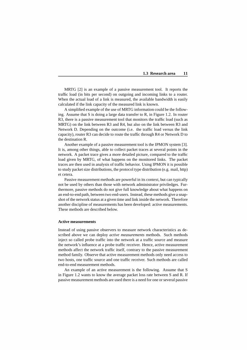
MRTG [2] is an example of a passive measurement tool. It reports thetraffic load (in bits per second) on outgoing and incoming links to a router.When the actual load of a link is measured, the available bandwidth is easilycalculated if the link capacity of the measured link is known.

A simplified example of the use of MRTG information could be the follow-ing. Assume that S is doing a large data transfer to R, in Figure 1.2. In routerR3, there is a passive measurement tool that monitors the traffic load (such asMRTG) on the link between R3 and R4, but also on the link between R3 andNetwork D. Depending on the outcome (i.e. the traffic load versus the linkcapacity), router R3 can decide to route the traffic through R4 or Network D tothe destination R.

Another example of a passive measurement tool is the IPMON system [3].It is, among other things, able to collect packet traces at several points in thenetwork. A packet trace gives a more detailed picture, compared to the trafficload given by MRTG, of what happens on the monitored links. The packettraces are then used in analysis of traffic behavior. Using IPMON it is possibleto study packet size distributions, the protocol type distribution (e.g. mail, http)et cetera.

Passive measurement methods are powerful in its context, but can typicallynot be used by others than those with network administrator priviledges. Fur-thermore, passive methods do not give full knowledge about what happens onan end-to-end path, between two end-users. Instead, these methods give a snap-shot of the network status at a given time and link inside the network. Thereforeanother discipline of measurements has been developed: active measurements.These methods are described below.

Active measurements

Instead of using passive observers to measure network characteristics as de-scribed above we can deployactive measurementsmethods. Such methodsinject so called probe traffic into the network at a traffic source and measurethe network’s influence at a probe traffic receiver. Hence, active measurementmethods affect the network traffic itself, contrary to the passive measurementmethod family. Observe that active measurement methods only need access totwo hosts, one traffic source and one traffic receiver. Such methods are calledend-to-end measurement methods.

An example of an active measurement is the following. Assumethat Sin Figure 1.2 wants to know the average packet loss rate between S and R. Ifpassive measurement methods are used there is a need for one or several passive


observers inside the network core. This requires control and administrativeprivileges on the network path between S and R. In an active measurement Sinsteadprobesthe network path between S and R by injecting a set ofprobepacketsinto the network (this is the active part of the measurement). Thesepackets traverse the network all the way to R where the packets are collected(at least the packets that were not lost). Note that neither Snor R knows theexact route through the network. That is, the packets traverse a black box thatyou cannot study directly. When all packets have been collected by R, a ratiodescribing the number of probe packets lost is sent back to S.Thus, S has asnapshot describing the loss rate on the path between S and R.

Probing is the basic element of all active measurement methods, includingmeasurements to gain information about link capacity and available bandwidthof a network path. There exist a variety of probing schemes. Below, two basicprobing schemes are described: the packet-pair and the packet-train probingschemes.

Probing schemes for bandwidth measurements

To estimate end-to-end available bandwidth or link capacity by active measure-ments the first step is to probe the network path. This is done by injecting a setof probe packets with a pre-defined separation ordispersion. The dispersionis inversely proportional to theprobe rate(measured in bits per second). Asmaller dispersion between probe packets is equivalent to ahigher probe rate.When the probe packets traverse the network, the pre-defineddispersion maychange. This is due to competing network traffic or to the so called bottleneckspacing effect[4].

The most basic probing scheme is to divide the probe packets in pairs; eachpair has a pre-defined dispersion that corresponds to the probe rate [5] [6] [7][8] [9] [10] [11]. Each pair is sent through the network to thereceiver wherethe packets are time stamped (usually at the application layer). The arrival-timestamps are used when the actual bandwidth estimate is calculated.

Instead of using pairs of probe packets many methods usetrains of probepackets [9][10][12][13][14]. The dispersion between the probe packets in-side the train can for example be equal or exponentially decreasing. There isa fundamental difference between using packet-pair and packet-train probingschemes. In packet-train probing schemes several probe packet delays may bedependent on each other, which is not the case in packet-pairprobing schemes[15].

Having the arrival times of the probe packets, an analysis can be performed

1.3 Research area 13

using the arrival times as input to obtain the estimate.

Analysis of active measurements

The analysis of results obtained from active measurements typically involvesstatistical operations on the dispersion values. To get an idea of how an anal-ysis is performed, a simplified version of Pathload [12] is described since thatalgorithm is intuitive. A more in-depth description of probing analysis is givenin Chapter 2.

A sender S is probing the path between S and R in Figure 1.2 using eithera packet-pair or a packet-train probing scheme. An initial dispersiondi (i.e.probe rate) is decided and thereafter the probe packets are injected into thenetwork. The initial dispersiondi may change on the path between S and R.The, by utilizing the statistical mean operator on the received dispersion valuessystem noise is filtered out. The analysis idea is the following:

1. if the received dispersion mean is equal todi the probe rate is below theavailable bandwidth

2. if the received dispersion mean is greater thandi the probe rate is abovethe available bandwidth

By sending probe pairs or probe trains at different probe rates (i.e. usingdifferent dispersion between probe packets) the availablebandwidth can bedetermined by binary search.

1.3.2 Link capacity and available bandwidth

To be able to develop a deeper understanding of the models andtools in thearea of bandwidth measurements, a strict definition of available bandwidth isneeded. The following definition of link capacity and available bandwidth istaken from [16].

The capacityC of a single link (between two routers) is defined as themaximum IP layer transfer rate. When data is encapsulated into IP packets,overhead is induced. That is, the maximum IP layer transfer rate is lowerthan the actual raw link transfer rate. From an application point of view, themaximum IP layer transfer rate is more interesting than the actual raw linktransfer rate since applications can not send data without data encapsulation.


The end-to-end link capacityC, havingH successive links, is defined asthe minimum capacity between the two nodes. That is,C = mini=1::H CiwhereCi is the capacity of linki.

The intuitive definition of the available bandwidth is the unused portionof the link capacity. However, this definition needs to be refined into a morestrict definition. The definition from [16] builds on the observation that thetransmission of bits (a bit is either 0 or 1) on a link is a discrete process. Eitherthe link is busy sending a bit or the link is idle. The average utilization of a linkcan be described as u(t1; t2) = 1t2 � t1 Z t2t1 d(x)dxwhered(x) is either 0 or 1 at a given timex. That is, the utilization of a linkdepends on the time interval.

The available bandwidth of a single link is defined asAi = (1� ui) � Ci.Further, the end-to-end available bandwidth of a path containing H links isdefined as the minimum available bandwidth:A = mini=1::HAiwhereAi is the available bandwidth on linki.

The utilization of a link depends on thecross traffic. Cross traffic is theregular traffic that flows through the network (i.e. all traffic but the probe trafficused in the measurement). Many parameters control the crosstraffic behavior,some described below:� Intensity distributionThe dispersion between cross-traffic packets can

be approximated by a probability function, such as rectangular (verysmooth), poisson or pareto (very bursty). Depending on the cross-trafficsource the intensity distribution may vary.� Packet size distributionDepending on the cross-traffic source the size ofthe packets will vary. For example, a transfer of a large file uses largepackets while a voice over IP application uses small packets.� Flow lengthThe cross-traffic flow between a specific sender and a re-ceiver may vary from short web traffic flows (measured in seconds) upto long flows corresponding to a file download (measured in hours).

1.3 Research area 15� AggregationThe cross-traffic on links within the core network is builtup of several cross-traffic flows. A higher number of cross-traffic flowsgives a higher degree of aggregation. Usually a high degree of aggrega-tion gives a more smooth overall cross-traffic intensity distribution.

There as been many attempts to describe cross traffic behavior (e.g. in[17]). Such studies are most often done using passive measurements. Thecross-traffic behavior changes over time, e.g., when new applications enter themarket. It is important to understand the cross-traffic behavior when simulatingcross traffic in network simulators and testbeds, discussedbelow.

1.3.3 Problems

One of the inherent complications in bandwidth measurementresearch is thatthe available bandwidth varies over time. This is a consequence of the vari-ability of the cross traffic over time. In Figures 1.5 and 1.6,two examples areshown. In Figure 1.5, the cross-traffic load (y-axis) is plotted with a resolutionof 5 minutes (x-axis) while in Figure 1.6 the resolution is 30minutes (x-axis).The shaded area corresponds to the traffic load on one outgoing link while theline corresponds to the traffic load on one incoming link. Theavailable band-width on each link is the link capacity minus the cross-traffic load.

Figure 1.5: MRTG day trace. 5 minute intervals.

Assume that the available bandwidth is estimated. A fast measurementmethod can, for example, measure the available bandwidth during the largecross-traffic load peek at 15.5 (x-axis) in Figure 1.5. This will give a very lowestimate of the available bandwidth. That value is not representative over other,longer time scales. Another method that probes a path duringa longer periodof time will get a higher estimate of the available bandwidth. However, in thiscase the cross-traffic peaks are invisible. Depending on theapplication that willuse the available bandwidth estimates, different approaches must be taken.


Figure 1.6: MRTG week trace. 30 minute intervals.

1.3.4 Testing and verification

It is important to be able to verify the bandwidth estimates obtained by bothnew and old measurement method. Three different techniquesused for methodtesting and verification are discussed. Testing and verification by network sim-ulations, by testbed measurements and by real network measurements. Eachmethod is described and discussed below.

Network simulations

Network simulators (such as NS-2 [18]) are software that simulate computernetworks. In such an environment, all parameters are known and hence are verywell suited for testing and verification of available bandwidth measurementmethods. Network topologies that are otherwise inaccessible to researchers canbe simulated. In these environments a model of the measurement method canprobe a simulated path and analyze the results to form a bandwidth estimate.Verification is simple, since the link capacity and available bandwidth are inputparameters to the simulator. Cross-traffic is usually generated either by a cross-traffic generator or by traffic traces (a packet log collectedfrom a real network).

The disadvantage of network simulations is that a simulation is a modelthat tries to represent the real world; in this case the simulation represents acomputer network with its software and hardware. To create amodel of acomputer network many simplifications have to be made, hencethere may bea gap between results obtained from network simulations andresults obtainedfrom real networks, especially if the scenario or the modelsare complex.

Furthermore, it can be difficult to make realistic scenarios. As one exam-ple, it is a known fact in the research community that it is hard to configure arealistic cross-traffic mix.

1.4 Our research 17

Testbed measurements

Testing and verification in testbed networks is a step towards testing and veri-fication in real networks. In testbed networks an opportunity to run real soft-ware that implements the bandwidth measurement method is given. It is on theother hand expensive to create large network topologies. Intestbed measure-ments the network topology, cross-traffic load and distribution et cetera canbe controlled. Cross traffic is usually generated by cross-traffic generators orby traffic traces. The problem of creating realistic cross-traffic mixes is thesame as in network simulations. Due to the control of all variables in testbedscenarios verification is simple.

Real network measurements

Usually, the developers of a new measurement methods want torun tests in areal network, such as the Internet. In large real networks itis hard to control thetopology or the cross traffic. However, verification is stillpossible using pas-sive measurements described in Section 1.3.1. For example,using MRTG [2]the current traffic load can be obtained on selected links on an end-to-end path(see Figures 1.5 and 1.6, both produced by MRTG). The cross-traffic load andthe link capacity give the actual available bandwidth during the measurement.That is, we can verify the estimate produced.

The problem with passive measurements in real networks is ofcourse thefact that most people do not have access to information collected in the corenetwork. Another problem is that not all routers collect traffic load data to bepresented in MRTG.

1.4 Our research

This section describes the research problems in the scope ofthis thesis, theresearch method and the contributions.

1.4.1 Research problems

Bandwidth estimation research has been in focus for quite some time and thearea is starting to mature. However, there still exist several research problemsthat are unsolved or needs to be addressed more carefully. Inthe thesis thefocus is on two important research problems. These are described below:

18 Chapter 1. Introduction� It is important to understand the process when cross traffic and probetraffic interacts on a network path. This has to be studied both fromthe perspective of the probing method and from the perspective of thecross-traffic. How does the cross-traffic affect probe traffic and how iscross-traffic affected by probe traffic?� Bandwidth measurements in wired networks, such as the Internet, hasgained quite a lot of attention. When new network technologies starts toappear and are adopted (such as 802.11, ad-hoc networks, GPRS, 3G)it is important to investigate whether current bandwidth measurementmethods are applicable in these new settings, with or without modifica-tion.

Other equally important research problems that need further attention aredescribed in a set of bullets below1:� Evaluation and comparison of existing bandwidth measurement tools. Is

there a need for benchmarks to compare tools and methods against eachother?� There is a need to lower the amount of probe traffic send between a probesender and a probe receiver but still keep the accuracy of themeasure-ment method. This is due to the fact that probe traffic affect other trafficflows in the network, often negatively.� Create stronger links between bandwidth estimation and TCPresearch.� Continuous measurements of the available bandwidth of a network path:instead of measuring once and then use that estimate in an applicationthere is a need for continuous measurements over large time periods.� Coordination of several end-to-end measurements between different end-nodes in order to depict the current status of an entire network.� Incorporation of bandwidth measurement research results into real ap-plications. What are the applications that can benefit from results in thebandwidth measurement research area? What new problems andrestric-tions have to be considered in the specific case?� Methods for bandwidth prediction.

1these research problems were discussed at the Bandwidth Estimation Workshop held in SanDiego, 2004.

1.4 Our research 19

1.4.2 Research method

This section describes the research method used to go from the research prob-lems above to the contributions described below.

The dominating research method in the computer science areadiscussedin this thesis is experimental. That is, the study of cause and effect. A setof hypotheses describing a system or a phenomenon are testedby conductingexperiments. Thereafter conclusions are drawn which in turn will lead to newhypotheses.

In the thesis the interaction between cross-traffic and probe-traffic packetsis studied. Further, the thesis presents an evaluation of tools and methods forestimating end-to-end available bandwidth and link capacity in new scenarios.These two research problems correspond to two branches of the experimentalscience. The first branch, to study packet interaction is more or less funda-mental science while the study and evaluation of tools and methods are appliedexperimental research. Both branches will hopefully lead to new and bettermethods and tools.

Independent of the branch of experimental research methodology our pri-mary task is to isolate the effect of single variables. The important variablesin bandwidth estimation can be divided into two categories:system variablesand method variables. A system variable is a variable that affect the networkin-between a probe sender and a probe receiver. Such variables are for exam-ple cross-traffic load and distribution on each link betweenthe sender and thereceiver, router queues and policies. A method variable is avariable that istightly bound to the actual method. Examples are the probingscheme, the totalnumber of bits to be transferred, the analysis method et cetera. Depending onthe verification method (described in 1.3.4), a subset of these variables can befixed and controlled.

To obtain validity there is a need for verification of the experiments. De-pending on the verification method (described in section 1.3.4) we can achieveeverything from low to high validity.

Another aspect of experimental research methodology is thereproducibilityof the study. By conducting experiments in network simulations and in testbedsand then documenting all parameters the experiments can be repeated withsimilar results. Experiments in real networks, such as the Internet, are harder toreproduce, however such measurements can be verified (as described in 1.3.4).


1.4.3 Contributions

This section presents the main contribution of the thesis. The results are di-vided into four papers, each individual paper is presented in the second part ofthe thesis. A summary of the papers can be found in Chapter 3.� Packet interaction framework:A framework has been developed that

describes, at the discrete packet level, how probe-packet trains and cross-traffic packets interact with each other when traversing a network path.Using this framework the differences between using the meanand themedian operator on dispersion values obtained from active probing isdiscussed.� DietTopp: Within the scope of the thesis DietTopp has been developedand implemented. DietTopp is a bandwidth estimation tool that is basedon a modification of the previously not implemented TOPP method.� Combination of ad-hoc networks and bandwidth estimation:The thesisillustrate and discuss four research problems associated with the combi-nation of active bandwidth measurements and ad-hoc networks: variablemeasured link capacity, moving nodes, loss rate and time control.� Wireless measurements:We show that both the measured link capacityand the available bandwidth decrease with decreasing probepacket size.Further, we show show that both the measured link capacity and theavailable bandwidth decrease with increasing cross-traffic rate.

Chapter 2

Related work

2.1 Introduction

Much work has been done in the bandwidth estimation area during the recentyears. In this section the emphasis is on state-of-the-art bandwidth measure-ment tools, measurements in wireless networks and applications of bandwidthestimation. A short review of the more theoretic literatureis given below.

Many studies of the underlying theories for probe packet interactions withrouters, queues and cross traffic have been developed. In [8]a discussion ofhow the packet size affects the estimation of link capacity is made. Further-more, they describe a model for probe packet delay variation. This modelformalizes the packet-pair method concept.

In [9][19], theories and a discussions of link capacity measurements aregiven. What are the problems with variable packet size probing (describedin subsection 2.2.1) and what are the alternatives? This work also describesPathrate, a tool for measuring the end-to-end minimum link capacity. Further,[10][20] gives theoretical discussions about what packet-pair techniques mea-sure, in the context of available bandwidth. This work also describes the avail-able bandwidth estimation tool Pathload. In [16], common misunderstandingswhen designing bandwidth estimation tools are discussed.

Discussions about packet-pair methods have also been made in [11][13],which also describe the TOPP algorithm.

The problem of obtaining accurate time stamps for probe packets has beendiscussed in [21]. This is a very important problem, especially in high speednetworks, since all analysis methods rely on accurate time stamps.

21

22 Chapter 2. Related work

2.2 Bandwidth measurement tools

A large number of bandwidth measurement tools have been developed sinceKeshav’s first attempt to measure the available bandwidth. In this section a de-scription of the two main available bandwidth estimation categories are givenalong with a few examples. The main available bandwidth estimation cate-gories arepacket rate methodsandpacket gap methods(notation used in e.g.[22]).1

Also, a brief introduction to link capacity estimation is given. These meth-ods either estimate the minimum link capacity of an end-to-end path, or thecapacity of each hop. Here the emphasis is on a description ofa hop-by-hopmethod.

It should be noted that a comparison of the method and tool performanceis left out, since such a work is a study of its own. In [23], theproblems ofcomparing bandwidth measurement tools is discussed.

2.2.1 Packet rate methods

The basis of the packet rate methods is so called self-induced congestion. Theidea is the following: inject a set of probe packets (e.g. in pairs or in trains)with a predefined initial probe rate into a network. If the initial probe rate ishigher than the available bandwidth, the probe packets willbe queued aftereach other at the bottleneck and thus cause congestion. In such a case, themean dispersion between the probe packets will increase, which is equivalentto a decrease in the received probe rate. However, if the initial probe rate isequal to the received probe rate it is assumed that the packets did not have toqueue and thus the end-to-end path is not congested. That is,the initial proberate is less than the available bandwidth.

There exist several tools that exploit this phenomenon, such as Bart [24],Pathchirp [14], Pathload [12] and TOPP [11]. To illustrate packet rate methodsa deeper introduction to Pathload and Pathchirp is given below. A descriptionof TOPP can be found in part two of this thesis.

Pathload

Pathload is an implementation of the Self-Loading PeriodicStreams (SLoPS)methodology [12][20]. Using this methodology the end-to-end available band-width is measured. The basic idea of SLoPS is explained below.

1These categories are called iterative probing and direct probing, respectively, in [16].

2.2 Bandwidth measurement tools 23

A sender transmits a packet train with a pre-defined probe rate to a receiver.The sender time stamps the send time while the receiver time stamps the probepacket reception. The time stamp difference, defined as theone way delay(OWD) is calculated for each packet (D1; D2; :::; DK).

If the initial rate is higher than the available bandwidth, the router queuewill grow when additional probe packets in the train are received to the router.Due to this fact, the OWD values will have an increasing trend(i.e. DK >DK�1 > ::: > D1). When the initial probe rate is less than the availablebandwidth, the router queues will not grow due to the injection of the probetrain. Hence, the OWD will be more or less stable. Statistical tests are used todetermine whether the OWD values are stable or increasing.

By sending probe trains at different pre-defined probe rates, the availablebandwidth is found by binary search. If the initial probe rate causes an increas-ing OWD trend the probe rate is above the available bandwidth. The probe-train rate for the next train is decreased. On the other hand,if the probe traindoes not cause an increasing OWD trend, the initial probe rate is less than theavailable bandwidth. In this case the probe rate is increased. This process isiterated until a satisfactory accuracy of the available bandwidth is obtained.

Pathchirp

Queuing delay

Packet send time

Excursion 1 Excursion 2

Figure 2.1: Packet sending time versus queuing delay by Pathchirp.

Pathchirp is another tool that measures the end-to-end available bandwidthand exploits the packet rate method. Instead of sending probe packet trainsit sendschirps of probe packets. A chirp is essentially a packet train, butthe dispersion between the probe packets are exponentiallydecreasing,dn =T n; d(n � 1) = T (n � 1); :::; d(2) = T 2; d1 = T 1, wheredi is the


dispersion andT and are constants. By using chirps the end-to-end path isprobed at different initial probe rates using just one train.

In the analysis the probe packet sending time is compared to the queuingdelay that arises when the initial probe rate is above the available bandwidth.The queuing delay is derived from comparing probe packet send and receivetimes. In Figure 2.1 an example plot is shown, describing themeasurementresult obtained from one chirp. When the queuing delay is zero, the probepackets were transmitted without queuing. During the excursions, shown inthe figure, the cross traffic is more intensive and hence causes queuing. Thefirst few excursions go back to zero because the cross traffic is bursty (i.e.sometimes the cross traffic is absent during a chirp). The last excursion in thefigure does not return to zero. This is when the send probe ratehas exceededthe bottleneck link capacity.

By analyzing the excursions from many chirps, Pathchirp is able to forman estimate of the end-to-end available bandwidth.

2.2.2 Packet gap methods

When using packet gap models the network topology must be known to someextent, usually the bottleneck link (i.e. the link that determines the availablebandwidth) must be known. Further, there can only be one bottleneck linkbetween the probe sender and the probe receiver.

Packet gap methods solve the following equation:A = Cbl �Ri(CblRo � 1)whereCbl is the link capacity of the bottleneck link (that is known),Ri

is the initial probe rate andRm is the measured probe rate. To obtain valuesof Ri andRo, the end-to-end path is probed using different initial probe rates.For each probe train or probe pair an estimate of the available bandwidth canbe made.

Sometimes the equation above is expressed using time (in seconds) insteadof rates (in bits / second). But the result is still the same.

Examples of tools exploiting the packet gap method are Delphi [25] andSpruce [22].

2.2 Bandwidth measurement tools 25

2.2.3 Link capacity estimation

The two measurement categories above describe how to estimate the availablebandwidth. Much effort on developing link capacity measurement tools hasalso been made. Many such tools rely on variable packet size probing. Thefirst tool to implement this method was Pathchar [26] which estimates the linkcapacity on each hop between two nodes. It should be noted that Pathchar doesnot need a receiver node. Other tools followed in the same track, such as pchar[27]. The basic idea of Pathchar is discussed next.

Pathchar

IP packets, and thus probe packets, contain a time to live (TTL) field. TTL is anumber, specified by the sender, which is decremented by eachrouter in a path.If the TTL is low, or the path contains many routers the TTL mayreach zero. Insuch case the packet is dropped and an Internet Control Message Packet (ICMPtime exceeded packet) is sent from the router to the sending node.

By sending probe packets with a TTL ofn the round trip time (RTT) toroutern can be estimated. The RTT to routern can be expressed asRTT = nXi=1( pCi + li)

wherep is the size of the probe packet,Ci the capacity of linki andli thelatency of the ICMP packet on linki.

By sending probe packets with different TTL values an estimate of the RTTto both routern andn�1 is obtained. Further, by subtracting the RTT to routern� 1 from the RTT to routern we obtain the RTT for the hop betweenn andn � 1. In [26] it is stated that the relation between the minimum RTT (i.e.where probe packets did not have to queue in routers) and the probe packetsize is linear for each linki in the path. The following equation describes thatrelation: RTT = �+ � � p

where� is the sum of the ICMP latency and� is the sum of 1Ci for eachlink i (i.e. the slope of the minimum RTT whenp changes).

Thus, by sending probe packets with different sizes for eachfixedn-value,the parameters of the straight line can be calculated. Having that relation, thecapacityCi of each hop is obtained.


New methods

In [19], it is discussed why the methods that rely on variablepacket size prob-ing often lead to inaccurate estimates. For example, it is not always possibleto estimate the minimum RTT. Pathrate [28] is a modern link capacity tool thatestimates the minimum link capacity on an end-to-end path. It requires botha sender and a receiver and hence is less flexible. However thelink capacityis estimated with higher accuracy than previous methods. Pathrate relies onpacket-pair and packet-train probing instead of using ICMPinformation fromthe routers.

TOPP [13] is another tool that estimates the bottleneck linkcapacity of anend-to-end path. This method also needs a sender and receiver part. A modifi-cation of TOPP is implemented in a tool called DietTopp whichis described inpaper C and paper D.

2.3 Measurements in wireless networks

To date, not many studies have been made on applying active bandwidth mea-surements in wireless networks. In [29] a description of theeffect of variableprobe packet sizes in wireless networks is given. In that study they have eval-uated bandwidth measurement tools in a testbed scenario with simple crosstraffic. That study is extended in paper D of this thesis.

[30] describes a model to calculate the available bandwidthbetween twonodes in an ad-hoc network2. However, the available bandwidth is calculatedwith the help of the intermediate nodes. In paper B a discussion of the problemsof end-to-end available bandwidth measurement methods is given.

2.4 Applications of bandwidth measurements

There exist many potential applications of bandwidth measurement methods.For example: streaming media adaptation, server selection, network tomogra-phy, TCP improvement and service-level-agreement verification. This sectiondiscusses and describes these applications and the potential benefit that activemeasurements could give.

2An ad-hoc network is a wireless spontaneously connected network without pre-defined infras-tructure.

2.4 Applications of bandwidth measurements 27

Streaming media

The send rate and video quality adaptation of streaming media is important,especially when services like TV over the Internet is becoming more popular.Today, the adaptation is typically based on packet loss rateor delay. If thereis a method to adapt, in real time, the send rate and video quality to the avail-able bandwidth, the problem of congestion in the network maybe minimized.Most current available bandwidth methods are not applicable here, since theymeasure the available bandwidth at one point in time. However, the tool Bart[24] continously measure the available bandwidth. Future research is neededto combine streaming media and available bandwidth measurement tools.

Server selection

Server selection is another important application. That is, which server givesme, as a user, the shortest download time? If the available bandwidth could bemeasured in a quick and easy manner for many mirror servers (i.e. servers thatcontain the same data) at the same time, a user would be able tochoose thebest alternative. Further research in this area may lead to less congestion if thetotal traffic load can be spread out among the servers.

Network tomography

Network tomography is about trying to describe and map a network by ac-tively measuring the characteristics from many end-pointsat the same time.It is important to understand how available bandwidth bottlenecks are sharedbetween different end-hosts and to study how the available bandwidth bottle-necks change and perhaps move to a different location over time. Networktomography is also interesting from a router perspective: if the routers have aglobal view of the available bandwidth bottlenecks they maybe able to routethe traffic around congested links.

Some research has been done in this area [31][32]. The research is promis-ing but has to cope with slow measurement techniques. If several slow mea-surement techniques have to be synchronized, the entire network tomographymeasurement will in turn be very slow. Another problem is theidentificationof bottleneck links, that is how to determine that a bottleneck link is sharedbetween two paths.


TCP improvement

TCP is a transport protocol that tries to adapt the send rate to the current avail-able bandwidth. Many TCP versions have been developed, eachwith its ownspecific twist.

An example where active measurement techniques have been adopted isfound in [33]. In this work the startup algorithm, usually the TCP slow startmechanism, uses bandwidth measurement techniques. The available band-width is estimated using the trains of packets that flow from the sender to thereceiver in the initial phase. Observe that the packets are part of the data thatis transferred. After just a few round trip times the TCP has an initial value ofthe available bandwidth. Thereafter the send rate can be adapted in the usualTCP way.

TPTEST

TPTEST [34] is a service-level-agreement verification toolthat relies on activemeasurements from an end-user to a measurement server located inside thenetwork. TPTEST uses TCP throughput as the metric. As described in forexample [16], TCP throughput is not a good metric for available bandwidth.However, TPTEST is used as a tool for comparative analysis. That is, usersshould be able to compare results from using one network operator with resultsfrom using another operator. When all measurements are doneusing the samemetric, it might be a fair comparison.

Chapter 3

Summary of papers

This section summarizes the main contribution of each paperincluded in thisthesis. My contribution to each paper is also marked out. BobMelander andMats Bjorkman are co-authors of all papers. Both have guided me, discussedthe research issues and written parts of each paper. Bob Melander has alsoco-developed the measurement tool DietTopp as well as the NS-2 framework.The following papers are included in the thesis:

3.1 Paper A

“On the Analysis of Packet-Train Probing Schemes”, AndreasJohnsson, BobMelander and Mats Bjorkman, In Proceedings to the International Conferenceon Communication in Computing, Special Session on Network Simulation andPerformance Analysis, Las Vegas, June 2004.

Summary This paper describes probe packet and cross-traffic packet inter-actions at the discrete packet level. We identify three maininteraction-typeswhich we call mirror patterns, chain patterns and quantification patterns, re-spectively. Experiments have been performed in a testbed tounderstand andexplore the behavior of these patterns and how they affect bandwidth measure-ment results. The paper ends with a description of the difference, using thepatterns, between using the mean operator and the median operator on mea-surement values obtained during the probing phase.

29

30 Chapter 3. Summary of papers

My contribution I have co-developed the measurement tool used in the pa-per, I have performed all experiments and written most partsof the paper.

3.2 Paper B

“A Study of Dispersion-Based Measurement Methods in IEEE 802.11 Ad-hocNetworks”, Andreas Johnsson, Mats Bjorkman and Bob Melander, In Proceed-ings to the International Conference on Communication in Computing, SpecialSession on Network Simulation and Performance Analysis, Las Vegas, June2004.

Summary In this paper we study the effect of multiple-access networks ondispersion-based measurement methods. We especially focus on 802.11b net-works. We discuss four important research problems in this area: variablemeasured link capacity, movement of wireless nodes, packetloss rate and tim-ing issues. Using simulations in NS-2 we show that the measured link capacitydepend on the current cross-traffic intensity. Furthermorewe briefly discusswhat happens when the path between the two end-nodes changes(i.e. whenwireless nodes move around). We discuss the impact of packetloss in wire-less networks and how available bandwidth measurement methods may adaptto that. Finally we discuss problems with jitter when sending probe packets ina multiple-access network. This paper is a work-in-progress paper and hencedoes not provide any experimental or measurement results.

My contribution I have co-developed the experiment platform in NS-2, Ihave performed all experiments and written most of the paper.

3.3 Paper C

“DietTopp: A First Implementation and Evaluation of a Simplified BandwidthMeasurement Method”, Andreas Johnsson, Bob Melander and Mats Bjorkman,In Proceedings to the Second Swedish National Computer Networking Work-shop, Karlstad, November 2004.

Summary This paper describes an implementation of DietTopp, which is amodification of the TOPP method for measuring end-to-end available band-width and link capacity. We evaluate the DietTopp implementation in a testbed

3.4 Paper D 31

where one of the links is congested during the measurement session. We com-pare our results to both Pathload (that measures end-to-endavailable band-width) and Pathrate (which measures the end-to-end link capacity) with promis-ing results.

My contribution I have constructed the testbed, co-developed the DietToppimplementation, performed all experiments and written most of the paper.

3.4 Paper D

“Bandwidth Measurements in Wireless Networks”, Andreas Johnsson, BobMelander and Mats Bjorkman, Submitted for publication.

Summary In this paper we have used DietTopp to explore the effects ofwireless bottlenecks on bandwidth measurement results. Weshow using ex-periments that both the measured link capacity and available bandwidth de-pends on the probe packet size when conducting bandwidth measurements inwireless networks. Furthermore we also show that the measured link capac-ity decreases with increasing cross-traffic rate on the wireless bottleneck. Wehave performed experiments with three different cross-traffic distributions, andwith several cross-traffic sources to validate our findings.The obtained resultsare also compared to results obtained from Pathload (a tool that measures theend-to-end available bandwidth). We describe a simple method for identifica-tion of wireless bottlenecks. Finally, we discuss the observation that bandwidthmeasurement results will be application dependent.

My contribution I have constructed the testbed, co-developed the DietToppimplementation, performed all experiments and written most of the paper.

Chapter 4

Conclusions and future work

There are several foci in this thesis. The first is on enhancing the foundationsof bandwidth measurement methods and the impact of cross traffic on probepackets. A framework for describing interactions, at the discrete packet level,between probe-train packets and cross-traffic packets has been developed. Us-ing this framework the differences between using the mean and the medianoperator on obtained dispersion values are explained.

Further, an evaluation of bandwidth measurement methods inboth wiredand wireless networks has been performed. Several characteristics that differbetween wired and wireless networks (including ad-hoc networks) have beenidentified from the available bandwidth measurement perspective. Using ourown tool, DietTopp, we show that both the measured link capacity and theavailable bandwidth decrease with increasing cross trafficor decreasing probepacket sizes.

The differences between performing available bandwidth measurements inwired and wireless networks have been investigated in this thesis. Future workis to investigate whether old bandwidth estimation methodscan be adapted tofit the needs in wireless networks. Perhaps, new algorithms and methods haveto be developed. Further, the problems of probing in ad-hoc networks will bestudied in more detail to give concrete solutions to the stated problems.

Investigation of active continuous bandwidth monitoring is also of great im-portance. Mathematical algorithms for continuous measurements will be triedout and evaluated. Continuous monitoring methods will for example be usedin streaming video applications. Continuous monitoring will also be studiedand evaluated in ad-hoc networks where the topology and available bandwidth

33

34 Chapter 4. Conclusions and future work

may change both drastically and frequently.A study of how probe traffic is treated by so called network shapers will

be done. There is a belief that network shapers treat networktraffic generatedfrom the various applications differently. In such a case, there is not only oneestimate of the available bandwidth of interest. Instead, the available band-width must be measured with the application protocol in mind.

Bibliography

[1] Larry L. Peterson and Bruce S. Davie.Computer Networks. MorganKaufmann, 2000.

[2] Mrtg - multi router traffic grapher. Web resource: http://www.mrgt.org.

[3] C. Fraleigh, S. Moon, B. Lyles, C. Cotton, M. Khan, D. Moll, R. Rockell,T. Seely, and C. Diot. Packet-level traffic measurement fromthe sprint ipbackbone. InIEEE Network Magazine, November 2003.

[4] Van Jacobson. Congestion avoidance and control. InProceedings of ACMSIGCOMM, pages 314–329, Stanford, CA, USA, August 1988.

[5] Srinivasan Keshav. A control-theoretic approach to flowcontrol. InPro-ceedings of ACM SIGCOMM, pages 3–15, Zurich, Switzerland, Septem-ber 1991.

[6] Robert Carter and Mark Crovella. Measuring bottleneck link speed inpacket-switched networks. Technical Report 1996-006, Boston Univer-sity Computer Science Department, Boston, MA, USA, March 1996.

[7] Kevin Lai and Mary Baker. Measuring bandwidth. InProceedings ofIEEE INFOCOM, pages 235–245, New York, NY, USA, March 1999.

[8] Attila Pasztor and Darryl Veitch. The packet size dependence of packetpair like methods. InTenth International Workshop on Quality of Service(IWQoS 2002), Miami Beach, USA, May 2002.

[9] Constantinos Dovrolis, Parameswaran Ramanathan, and David Moore.Packet dispersion techniques and capacity estimation. InIEEE/ACMTransactions on Networking, December 2004.

35

36 Bibliography

[10] Constantinos Dovrolis, Parameswaran Ramanathan, andDavid Moore.What do packet dispersion techniques measure? InProceedings of IEEEINFOCOM, pages 905–914, Anchorage, AK, USA, April 2001.

[11] Bob Melander, Mats Bjorkman, and Per Gunningberg. A new end-to-endprobing and analysis method for estimating bandwidth bottlenecks. InProceedings of IEEE Globcom, San Francisco, November 2000.

[12] Manish Jain and Constantinos Dovrolis. Pathload: a measurement toolfor end-to-end available bandwidth. InPassive and Active Measurement(PAM) Workshop 2002 Proceedings, pages 14–25, Ft Collins, Co, USA,March 2002.

[13] Bob Melander, Mats Bjorkman, and Per Gunningberg. Regression-basedavailable bandwidth measurements. InProceedings of the 2002 Interna-tional Symposium on Performance Evaluation of Computer andTelecom-munications Systems, San Diego, CA, USA, July 2002.

[14] Vinay Ribeiro, Rudolf Riedi, Richard Baraniuk, Jiri Navratil, and LesCottrell. pathchirp: Efficient available bandwidth estimation for networkpaths. InPassive and Active Measurement Workshop, 2003.

[15] Andreas Johnsson, Bob Melander, and Mats Bjorkman. Modeling ofpacket interactions in dispersion-based network probing schemes. Tech-nical report, Maalardalen University, 2004.

[16] Manish Jain and Constantinos Dovrolis. Ten fallacies and pitfalls on end-to-end available bandwidth estimation. InInternet Measurement Confer-ence, October 2004.

[17] Yongmin Choi, Heung-No Lee, and Anurag Garg. Measurement andanalysis of wide area network (wan) traffic. InSCS Symposium on Per-formance Evaluation of Computer and Telecommunication Systems, July2000.

[18] The network simulator - ns-2. http://www.isi.edu/nsman/ns/.

[19] R.S. Prasad, C. Dovrolis, and Bruce A. Mah. The effect oflayer-2store-and-forward devices on per-hop capacity estimation. Proceedingsof IEEE Infocom 2003, San Francisco, CA, April 2003.

Bibliography 37

[20] Manish Jain and Constantinos Dovrolis. End-to-end available bandwidth:Measurement methodology, dynamics, and relation with TCP throughput.In Proceedings of ACM SIGCOMM, Pittsburg, PA, USA, August 2002.

[21] Attila Pasztor and Darryl Veitch. Precision based precision timing with-out GPS. InProceedings of ACM SIGMETRICS, Marina Del Rey, CA,USA, June 2002.

[22] Strauss, Katabi, and Kaashoek. A measurement study of available band-width estimation tools. InACM SIGCOMM Internet Measurement Work-shop, 2003.

[23] Federico Montesino-Pouzols. Comparative analysis ofactive bandwidthestimation tools. InPassive and Active Measurement (PAM) Workshop,2002.

[24] Svante Ekelin and Martin Nilsson. Continuous monitoring of availablebandwidth over a network path. InSwedish National Computer Network-ing Workshop, Karlstad, Sweden, 2004.

[25] Vinay Ribeiro, Mark Coates, Rudolf Riedi, Shriram Sarvotham, BrentHendricks, and Richard Baraniuk. Multifractal cross-traffic estimation.In Proceedings of ITC Specialist Seminar on IP Traffic Measurement,Modeling and Management, Monterey, CA, USA, September 2000.

[26] Allen B. Downey. Using pathchar to estimate Internet link characteristics.In Proceedings of ACM SIGCOMM, pages 241–250, Cambridge, MA,USA, August 1999.

[27] Bruce Mah. pchar: A tool for measuring Internet path characteristics,June 2001. http://www.employees.org/~bmah/Software/pchar/.

[28] Pathrate - a measurement tool for the capacity of network paths.http://www.cc.gatech.edu/fac/Constantinos.Dovrolis/pathrate.html.

[29] Karthik Lakshminarayanan, Venkata N. Padmanabhan, and Jitendra Pad-hye. Bandwidth estimation in broadband access networks. InIn Proceed-ings to the Internet Measurement Conference, 2004.

[30] Hwa-Chun Lin and Ping-Chin Fung. Finding available bandwidth in mul-tihop mobile wireless networks. InProceedings of the IEEE VehicularTechnology Conference, Tokyo, Japan, 2000.

[31] Ningning Hu, Li (Erran) Li, Zhuoqing Morley Mao, Peter Steenkiste, andJia Wang. Locating internet bottlenecks: algorithms, measurements, andimplications. InSIGCOMM ’04: Proceedings of the 2004 conferenceon Applications, technologies, architectures, and protocols for computercommunications, 2004.

[32] Alok Shriram and Jasleen Kaur. Identifying bottlenecklinks using dis-tributed end-to-end available bandwidth measurements. First ISMABandwidth Estimation Workshop (BEst), San Diego, 2003.

[33] Ningning Hu and Peter Steenkiste. Improving tcp startup performanceusing active measurements: Algorithm and evaluation. InIn Proceedingsto the 11th IEEE International Conference on Network Protocols, 2003.

[34] TPTest. II-Stiftelsen, October 2002. http://www.iis.se/tptest/.

II

Included Papers

39

Chapter 5

Paper A:On the Analysis ofPacket-Train ProbingSchemes

Andreas Johnsson, Bob Melander and Mats BjorkmanIn proceedings to the International Conference on Communication in Comput-ing, Special Session on Network Simulation and PerformanceAnalysis, LasVegas, June 2004

41

Abstract

With a better understanding of how probe packets and cross-traffic packetsinteract with each other, more accurate measurement methods based on ac-tive probing can be developed. Several existing measurement methods rely onpacket-train probing schemes. In this article, we study anddescribe the inter-actions between probe packets and cross-traffic packets.

When one packet within a packet train is delayed, the dispersion (i.e. packetseparation) of at least two (and possibly more) probe packets will change. Fur-thermore, the dispersions are not independent, which may bias calculationsbased on statistical operations. Many methods use dispersion averages, such asthe mean, in the calculation of bandwidth estimates and predictions.

We describe cross traffic effects on packet trains. The interaction resultsin mirror, chain and quantification patterns. Experiments have been performedin a testbed to explore these patterns. In histograms of delay variations foradjacent probe packets, these patterns are manifested as different identifiablesignatures.

Finally, we also discuss the effect of these patterns on the mean and medianoperations.

5.1 Introduction 43

5.1 Introduction

Measurement of the end-to-end available bandwidth of a network path is get-ting increasingly important in the Internet. Verification of service level agree-ments, streaming of audio/video flows, and Quality-of-Service managementare all examples of Internet activities that need or can benefit from measure-ments of available bandwidth.

Many methods that attempt to measure end-to-end bandwidth actively probethe network path by injecting probe packets in predetermined flight patterns.Common flight patterns include pairs of probe packets, so called packet-pairprobing schemesand its extension into longer sequences of probe packets [1,2, 3, 4, 5, 6], which we will refer to aspacket-train probing schemes.

When the probe packets (independent of probing scheme) traverse the net-work path, the dispersion between successive probe packetswill change. Thisis due to limited link capacity and interactions with other packets traversing thesame path (so called cross-traffic packets).

To calculate an available bandwidth estimate an analysis ofthe dispersionvalues is made. The analysis relies on the probe packet dispersion at the senderside in combination with the probe packet dispersion at the receiver side.

In this article we describe the probe packet and cross-traffic packet inter-actions when using packet-train probing schemes. The interactions are mani-fested as patters. Further, we illustrate these patterns asidentifiable signaturesin histograms.

We describe the effect of the packet interactions when usingmean andmedian operations to dispersion values obtained from packet-train probingschemes. All dispersion-based measurements has been performed in a testbed,which is described in the article.

The rest of this article is organized as follows: Section 5.2describes threepatterns that occur when probe and cross-traffic packets interact with eachother. Section 8.2 defines a testbed that we have used for all of our measure-ments. Section 5.4 identifies four signatures that arise from the three patterns.Section 5.5 describes the impact of mean and median filteringwhen perform-ing analysis of dispersion values obtained from packet-train probing schemes.The article ends with conclusions in Section 8.5.

44 Paper A

5.2 Description of patterns

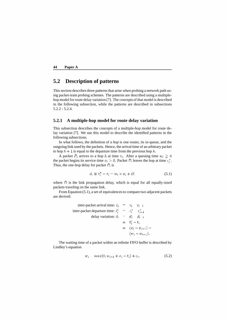
This section describes three patterns that arise when probing a network path us-ing packet-train probing schemes. The patterns are described using a multiple-hop model for route delay variation [7]. The concepts of thatmodel is describedin the following subsection, while the patterns are described in subsections5.2.2 - 5.2.4.

5.2.1 A multiple-hop model for route delay variation

This subsection describes the concepts of a multiple-hop model for route de-lay variation [7]. We use this model to describe the identified patterns in thefollowing subsections.

In what follows, the definition of ahop is one router, its in-queue, and theoutgoing link used by the packets. Hence, the arrival time ofan arbitrary packetto hoph+ 1 is equal to the departure time from the previous hoph.

A packetPi arrives to a hoph at time�i. After a queuing timewi � 0the packet begins its service timexi > 0. PacketPi leaves the hop at time��i .Thus, the one-hop delay for packetPi isdi � ��i � �i = wi + xi +D; (5.1)

whereD is the link propagation delay, which is equal for all equally-sizedpackets traveling on the same link.

From Equation (5.1), a set of equivalences to compare two adjacent packetsare derived:

inter-packet arrival time:ti � �i � �i�1inter-packet departure time:t�i � ��i � ��i�1

delay variation:Æi � di � di�1= t�i � ti= (xi � xi�1) +(wi � wi�1):The waiting time of a packet within an infinite FIFO buffer is described by

Lindley’s equation wi = max(0; wi�1 + xi � ti) + i; (5.2)

5.2 Description of patterns 45 i corresponds to the waiting time caused by cross traffic entering the hopbetween�i�1 and�i.

A router queue can in principle operate in two states - busy and idle state.The busy state implies that the router is constantly forwarding packets from itsin-queue, while in the idle state the in-queue is empty.

Probe packets (i.e. packets used for obtaining dispersion values) can conse-quently be divided into two categories,Initial andBusy probe packets (adapt-ing to the notation in [7]). The first packet of a busy period isby definition aninitial probe packet. That is, anI probe packet is never queued behind anotherprobe packet (i.e.wi of Equation (5.2) is equal to0 + i). B probe packets arepackets thatarequeued behind other probe packets.

With this categorization of probe packets, the delay variation Æi is definedwith respect to whether a probe packetPi is I or B. From [7] we have

I: Æi = (xi � xi�1) + (wi � wi�1) (5.3)

B: Æi = (xi � ti) + i (5.4)

where Equation (5.4) is derived from Equations (5.2) and (5.3).Equations (5.3) and (5.4) are extended in [7] to describe multiple hops.

These extensions are based on the following statements: if aprobe packet isI or B at hopj andB at hopj + 1, Æi is overwritten and replaced byÆi fromEquation (5.4). On the other hand, if the probe packet isI at hopj + 1, theright hand side of Equation (5.3) is added to the existingÆi.

Hence, a probe packet that traverses an H-hop path, beingI at every hop,has a delay variationÆi = HXh=1(xhi � xhi�1) + HXh=1(whi � whi�1): (5.5)

If a probe packet isB on at least one hop, it will beB for the last time atsome hop in the path. Denote this hopsi. The delay variation for such a probepacket is Æi = (xsii � ti + sii ) + HXh=si+1(xhi � xhi�1) ++ HXh=si+1(whi � whi�1): (5.6)

46 Paper A

5.2.2 Mirror pattern

In the following we will describe the characteristics of themirror pattern.Hence, consider a probe packet train, containing at least three probe packetsPi�1; Pi andPi+1 that are allI at hoph. Further, assume thatPi�1 andPi+1are unaffected by cross traffic (i.e.wi�1 = wi+1 = 0). Then, ifPi is delayed,wi > 0, its delay variationÆi > 0. Hence,Pi will have a delay variationÆi = (xi � xi�1) + (wi � wi�1) = (wi � wi�1), under the assumption of fixsize probe packets.

Since bothPi�1 andPi+1 are unaffected by cross traffic, the followingholds Æi+1 = wi+1 � wi= �wiÆi = wi � wi�1= wi=)Æi+1 = �Æi; (5.7)

which we define as aperfect mirror pattern. An example of this phe-nomenon is shown in Figure 5.1. The vertical packets above the time line showswhen in time a probe packet (white box) or a cross-traffic packet (shaded box)arrives to the hop. The arc indicates when in time all bits of the packet havebeen received to the router. When all bits have been received, the router trans-mit the packet on the outgoing link, if it is not delayed by another packet. Thetransmission from the router is shown below the time line in the same manneras above the time line. The horizontal packets describe the packet pattern onthe out-going link. Probe packetPi is delayedwi time units, visualized by thehorizontal arrow next toPi in Figure 5.1. SincePi�1 andPi+1 are unaffectedby cross traffic Equation (5.7) holds and we have a perfect mirror pattern.

In addition to the fact that probe packetPi can be delayed, there is a possi-bility that one, or both ofPi�1 andPi+1 are affected by cross traffic. This willcause changes to the mirror pattern as described below. It isobvious that thispossibility grows with increasing cross traffic and/or increasing probe rate.

Assume, for instance, that bothPi andPi+1 are delayed by cross traffic,while Pi�1 andPi+2 are unaffected. Then the mirror pattern isdivided in a

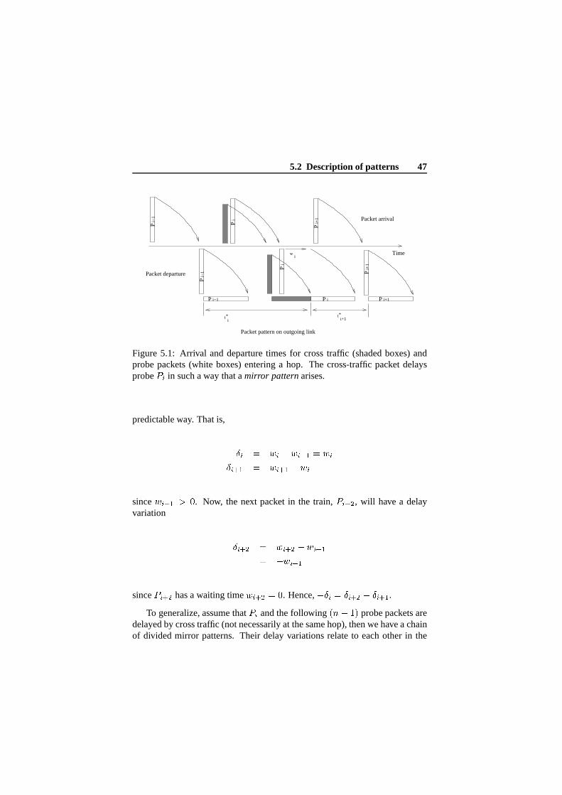
5.2 Description of patterns 47

Time

Packet departure

i−1

Packet pattern on outgoing link

i−1

i

it*

i+1 Packet arrival

iw

i+1t*

i−1 i

i+1

i+1i

P P P

P

P

P

P P P

Figure 5.1: Arrival and departure times for cross traffic (shaded boxes) andprobe packets (white boxes) entering a hop. The cross-traffic packet delaysprobePi in such a way that amirror patternarises.

predictable way. That is, Æi = wi � wi�1 = wiÆi+1 = wi+1 � wisincewi+1 > 0. Now, the next packet in the train,Pi+2, will have a delayvariation Æi+2 = wi+2 � wi+1= �wi+1sincePi+2 has a waiting timewi+2 = 0. Hence,�Æi = Æi+2 + Æi+1.

To generalize, assume thatPi and the following(n� 1) probe packets aredelayed by cross traffic (not necessarily at the same hop), then we have a chainof divided mirror patterns. Their delay variations relate to each other in the

48 Paper A

following way:Æi+n + � � �+ Æi+1 = (wi+n � wi+(n�1))+ � � �+ (wi+2 � wi+1)+(wi+1 � wi)= �wi= �Æi (5.8)=)i+nXa=i Æa = 0 (5.9)

sincewi+n = 0. That is, cross-traffic effects on packet trains will cancelout, toa certain degree, and hence not affect the mean value of the packet dispersionvalues (norÆ-values) obtained from the probe-packet train.

Mirror patterns are erased if probe packets in the packet train are trans-formed fromI to B, as described by Equations (5.5) and (5.6).

When a probe packet train traverses an H-hop path, the delay variationof every probe packet is described by Equation (5.5) or (5.6)depending onwhether the probe packets ever becomeB. We have extended the model pre-sented in [7] to describe the relation between delay variation values obtainedfrom packet-train probing.

5.2.3 Chain pattern

In this section we will describe the chain pattern. If a cross-traffic packet delaysa probe packet,Pi�1, in such a way that at leastPi andPi+1 are transformedfrom I to B, and makes the involved probe packetsPi�1, Pi andPi+1 back-to-back after the hop, a chain pattern is visible.

This is the definition of apure chain pattern. If other probe packets withinthe scope of the chain pattern are delayed by cross traffic, a quantification pat-tern will arise. Quantification patterns are described in Section 5.2.4.

An example of a chain pattern is shown in Figure 5.2, which is similar toFigure 5.1. WhenPi�1 is received, it must wait for the cross-traffic packet tocomplete its departure. The waiting time ofPi�1 iswi�1, shown in Figure 5.2.Pi�1 is transmitted back-to-back behind the cross-traffic packet. Pi�1 is in thisexample by definitionI since it does not have to queue behind any other probepacket.

5.2 Description of patterns 49


Time

i−1 i

i+1

w wi−1 i

Packet departure

Packet arrivali−

1

i−1 i i+1

i+1w

i

i+1

P P P

P P

P

P P P

Figure 5.2: Arrival and departure times for cross traffic (shaded boxes) andprobe packets (white boxes) entering a hop. The cross-traffic packet delaysPi�1 in such a way that achain patternarises.

During the waiting time ofPi�1, the next probe packetPi enters the router.Pi has to waitwi time units in the queue forPi�1 to complete its departure,and is thereforeB. After the waiting time,Pi is sent back-to-back behindPi�1.The same procedure is repeated forPi+1.

After the service time ofPi+1 has elapsed,Pi�1, Pi andPi+1 travel back-to-back after each other on the link. Also,Pi andPi+1 have been transformedfrom I to B since both packets had to queue behind other probe packets. Hence,a chain pattern is visible after the hop.

The relation between delay variation values from probe packets involved ina chain pattern can be described by Equation (5.8), similarly to mirror patterns.The difference is that the mirror pattern involvesI probe packets while thechain pattern involves probe packets that change fromI to B.

Chain patterns are preserved to some degree in an H-hop path if the hopwhere the patterns arise is the last hop where the probe packets areB. Ofcourse, this pattern is blurred by mirror and quantificationpatterns if thereare hops downstream hopsi with cross-traffic. This is described by Equations(5.5) and (5.6).

5.2.4 Quantification pattern

The last pattern identified in this paper is the quantification pattern. This patternis described below.

50 Paper A

Let us assume that the probe packet generator is sending probe packets at ahigh rate (i.e. the probe packet dispersion is less than the service timexCT of alarge cross-traffic packet). When a cross-traffic packet enters the router queuebetween the arrival time of two probe packets the probe packets will becomeseparated by the service timexCT of that cross-traffic packet. Hence thereis no idle time gap in the router between the probe packets. This separation ishereafter referred to as aquantification pattern. The term quantification is usedsince the traffic consists of discrete transmissions, rather than a continuous flowof bits.


Time

i−1

i−1

i+1

Packet departure

Packet arrival

i

wi−1

wi

wi+1

i−1

i

i+1

ctw

i i+1

P

P

P

P

P

P

PPP

Figure 5.3: Arrival and departure times of cross traffic (shaded boxes) andprobe packets (white boxes) entering a router. The upper left cross-trafficpacket causes a chain pattern. The smaller cross-traffic packet causes aquan-tification pattern.

An example of the quantification pattern is shown in Figure 5.3, which issimilar to Figure 5.1. In this example we see that the leftmost cross-trafficpacket creates a chain pattern (equivalent to Figure 5.2). The second cross-traffic packet entering the hop between probe packetPi�1 andPi will be sentdirectly afterPi�1, whilePi is sent back-to-back with the second cross-trafficpacket. Hence,Pi�1 has to waitwi�1 time units (stemming from the largecross-traffic packet), whilePi has to waitwi time units (corresponding to thesmall cross-traffic packet and a portion of the the big cross-traffic packet). Thatis, a quantification pattern has arisen.

The delay variation relation of values obtained from probe packets involvedin a quantification pattern can be described by Equation (5.8), similarly to mir-ror patterns.

Quantification patterns are preserved to some degree in an H-hop path if

5.3 Testbed setup 51

the hop where the pattern arise is the last hop where the probepackets areB.This pattern is blurred if there are hops downstream hopsi with cross-trafficnoise. This is described by Equations (5.5) and (5.6).

5.3 Testbed setup

The testbed network (see Figure 5.4) used in the experimentsconsists of threerouter nodes, one Black Diamond (BD) and two Torrent routers(T1 and T2)[8]. There are also a probing generator (PG), a probing receiver (PR), a trafficgenerator (TG) called IP Traf Gen (internal product of Ericsson,www.ericsson.com)and a traffic receiver (TR) which is an IXIA 1600 Traffic Generator/Analyzer.The links are all 100 Mbps except between the three routers, where the linksare limited to 10 Mbps.

PG BD T1

TG

TR

T2 PR10Mbps 10Mbps

Figure 5.4: Testbed setup

Depending on the experiment setup the cross traffic can enterand leave therouter chain at different positions. The cross traffic flow can be one or severalof the following: TG! T1 ! T2 ! TR (flow 1), TG! BD ! T1 ! TR(flow 2) and TG! BD! T1! T2! TR (flow 3).

All cross traffic is exponentially inter-packet spaced. Four different crosstraffic sizes where used: 64, 148, 482 and 1518 bytes. In the experiments all ofthese could be used at the same time or just a selection of them. When all sizesare used, 46% is of size 64, 11% of 148, 11% of 482 and 32% of size1518bytes. This distribution of packet sizes has its origin fromfindings in [9].

The cross traffic intensity is variable within the testbed, in steps of arbitrarysize.

The probe traffic is sent through the path PG! BD ! T1! T2! PR.The probe packet size is 1500 bytes and consists of 32 packets. Normally 5

52 Paper A

trains are sent per test run.

5.4 Signatures

When cross traffic affects a packet train, the train will suffer from differentpatterns, as discussed in Section 5.2. In this section we illustrate these patternsusing real packet trains which interact with cross traffic. The patterns, aloneor in combination with each other, correspond to different signatures. Thesignatures are described and illustrated in delay variation histograms below.

Four signatures are defined and discussed in this section. They are: inde-pendence, mirror, rate and quantification signatures. In [7] similar signatureshave been identifies for packet-pair probing schemes. However, we have shownthat packet-pair and packet-train probing schemes are fundamentally different[10]. Thus, it is important to identify the signatures for packet trains as well.Examples from the described testbed are shown.

The probe rate for each diagram in Figure 5.5 is 1 Mbps in the upper leftdiagram, 2.9 Mbps, 4.8 Mbps and 6.7 Mbps in the bottom right diagram. Theprobe packets are 1500 bytes, and are sent in 5 trains consisting of 32 packetsin each. The cross traffic rate is 5 Mbps, exponentially distributed and consistof 4 different packet sizes. The cross traffic uses flow 1 as described in Section8.2.

5.4.1 The independence signature

The independence signature is visible in scenarios where there is no or verylittle cross traffic interfering with the packet train. Thatis, no or very fewprobe and cross traffic packet interactions.

The signature arises from the fact that most probe packets traverse the net-work path unaffected by cross traffic, thus independent of other traffic. Thismeans that the delay variationÆ for such packets are near 0 as seen in the upperleft diagram in Figure 5.5. The peak atÆ = 0 is called the independence peak.

5.4.2 The mirror signature

The mirror signature is a signature that arises due to the mirror pattern. Ifthere is very little cross traffic and the probe rate is relatively low, there willarise mirror patterns in the values obtained from packet-train probing. That is,

5.4 Signatures 53

−6 −4 −2 0 2 4 6

x 10−3

0

10

20

30

40

50

delay variation (s)

#

−4 −2 0 2 4 6

x 10−3

0

5

10

15

20

25

30

35

40

delay variation (s)

#

−2 −1 0 1 2 3 4

x 10−3

0

2

4

6

8

10

12

14

delay variation (s)

#

−1 0 1 2 3 4

x 10−3

0

5

10

15

20

25

delay variation (s)

#

Figure 5.5: Using 4 packet sizes and cross traffic flow 1, with arate of 5 Mbps.The probe rate increases from approximately 1 Mbps (upper left) to 6.7 Mbps(lower right).

for each positive delay variation value there is a corresponding negative delayvariation value.

The upper right diagram of Figure 5.5 shows a distribution ofdelay varia-tion values around the diminished independence peak (compared to the upperleft diagram).

5.4.3 The rate signature

The rate signature is a peak that arises from the fact that several probe packetstraverse the network path back-to-back, because of the chain patterns. The ratesignature corresponds to the link rate of the link creating the chain pattern.

The rate peak grows in size when the probe rate increases, since more probepackets will travel back-to-back in such cases.

54 Paper A

The rate peak is visible in the bottom left diagram of Figure 5.5. The ratepeak is the leftmost peak. The delay variation value for thatpeak can be con-verted to the link rate.

5.4.4 Quantification signature

The quantification signature arises from the quantificationpattern describedabove. The quantification signature corresponds to the gap between probepackets. In the bottom right diagram of Figure 5.5 there are 3clearly sepa-rated regions of peaks. The leftmost peak corresponds to therate signature.

The locations of the quantification peaks depend on the size of the crosstraffic packets and the number of packets of each size that areinterfering.

5.5 Mean and median analysis using patterns

An important step in the analysis phase is to reduce noise andeffects stemmingfrom cross-traffic burstiness. One way to do this is to mean ormedian filterthe dispersion samples. It is therefore important to understand the impact andproperties of these statistical operations.

In a previous simulation-based study [10] we have shown thatthe patternsdescribed in Section 5.2 affect the mean and median. However, they are af-fected in different ways. These differences can be illustrated and explained interms of the packet interactions described as patterns in Section 5.2.

2 3 4 5 6 7 8 9 10 110.8

1

1.2

1.4

1.6

1.8

2

Probe rate (Mbps)

o/m

2 3 4 5 6 7 8 9 10 110.8

1

1.2

1.4

1.6

1.8

2

Probe rate (Mbps)

o/m

Figure 5.6: Mean offered / measured probe rate to the left. Median offered /measured probe rate to the right. Cross traffic = 3 Mbps on a 10 Mbps link.

5.5 Mean and median analysis using patterns 55

2 3 4 5 6 7 8 9 10 110.8

1

1.2

1.4

1.6

1.8

2

Probe rate (Mbps)

o/m

2 3 4 5 6 7 8 9 10 110.8

1

1.2

1.4

1.6

1.8

2

Probe rate (Mbps)

o/m

Figure 5.7: Mean offered / measured probe rate to the left. Median offered /measured probe rate to the right. Cross traffic = 5 Mbps on a 10 Mbps link.

Figures 5.6 and 5.7 show measurements from two different scenarios withincreasing amounts of cross traffic. The topology is described in Section 8.2with only cross traffic flow 1 being active. Both graphs in eachfigure show theratio between offered and measured dispersion rate on the y-axis. The x-axisis the probe rate. In the left side graphs mean filtering is used whereas medianfiltering is used in the right hand graphs. A ratio close to 1 corresponds to anunderload situation. In the part where a curve deviates from1, the slope usingmean filtering is inversely proportional to the link capacity [5].

From the graphs it is apparent that the mean and median filtering give dif-ferent results. When the probe rate increases the number of probe and cross-traffic packet interactions will also increase. These interactions will occur asmirror patterns followed in turn by chain and quantificationpatterns. In thecase of mean filtering, the asymmetry effects of the mirror and the chain pat-terns will be cancelled. Hence, they will have no effect on the offered / mea-sured ratio. The quantification patterns that arise when thelink is full (i.e.when the available bandwidth is reached) cause the slope of the curves seen inthe graphs regardless if mean or median filtering is used.

The symmetry effect of the mirror pattern is also cancelled with respect tomedian filtering. However, the asymmetry of chain patterns is not cancelled.The reason is that number of back-to-back probe packets constituting the chainpattern outnumbers the initial probe packet dispersion. Thus, the median isshifted towards the dispersion of back-to-back packets. Since the back-to-backchain corresponds to the measured probe rate whereas the offered rate corre-spond to the initial probe packet dispersion there will be a dip near 7 Mbps inthe median ratio curve in Figure 5.6.

Using the mathematical definitions of chain patterns it can be shown thatchain patterns can not occur until probing at 7 Mbps on a 10 Mbps link withan MTU of 1500 bytes.

Figure 5.7 shows an even more striking behavior when median filtering isapplied. The median filtering curve begins to rise at 5 Mbps because of quan-tification patterns that occur when the channel is full. At 7 Mbps there is a dropin the ratio curve caused by chain patterns. As before, thesechain patterns areinvisible when using mean filtering. When the probe rate is increased furtherthe quantification patterns will again dominate and hence cause a new rise ofthe median curve.

The two median curves has a chain saw shape near the availableband-width (7 Mbps in Figure 5.6 and 5 Mbps in 5.7) compared to the mean curves.Exactly why this happens is ongoing research. We also study if there is a possi-bility to combine the information from mean and median curves to make betterestimates of the available bandwidth.

5.6 Conclusions

In this article we have identified and described patterns that arise when probepackets and cross-traffic packets interact with each other.Further, we haveidentified signatures that originate from these patterns. We have studied howthese patterns and their corresponding signatures affect mean and median oper-ations that are used in the analysis phase of available bandwidth measurementmethods. All measurements in this article has been made in a testbed.

Our goal is to further study the patterns and the corresponding signaturesderived from dispersion values obtained from packet-trainprobing schemes.We will study mean and median operations and especially the combination ofthem to make better estimates of available bandwidth and link capacity on anend-to-end path.

Bibliography


[2] Constantinos Dovrolis, Parameswaran Ramanathan, and David Moore.What do packet dispersion techniques measure? InProceedings of IEEEINFOCOM, pages 905–914, Anchorage, AK, USA, April 2001.

[3] Srinivasan Keshav. A control-theoretic approach to flowcontrol. InPro-ceedings of ACM SIGCOMM, pages 3–15, Zurich, Switzerland, Septem-ber 1991.

[4] Kevin Lai and Mary Baker. Measuring bandwidth. InProceedings ofIEEE INFOCOM, pages 235–245, New York, NY, USA, March 1999.



[7] Attila Pasztor and Darryl Veitch. The packet size dependence of packetpair like methods. InTenth International Workshop on Quality of Service(IWQoS 2002), Miami Beach, USA, May 2002.

[8] Rikard Holm. Probe-based load measurement. Master thesis, EricssonResearch, Sweden, 2003.

57


[10] Andreas Johnsson, Bob Melander, and Mats Bjorkman. Modeling ofpacket interactions in dispersion-based network probing schemes. Tech-nical report, Maalardalen University, 2004.

Chapter 6

Paper B:A Study of Dispersion-basedMeasurement Methods inIEEE 802.11 Ad-hocNetworks

Andreas Johnsson, Mats Bjorkman and Bob MelanderIn proceedings to the International Conference on Communication in Comput-ing, Special Session on Network Simulation and PerformanceAnalysis, LasVegas, June 2004

59

Abstract

In this article we discuss how dispersion-based measurements are affected bymultiple-access networks, such as IEEE 802.11-based ad-hoc networks. Westudy four topics: variable link capacity, movement of wireless nodes, loss rateand timing issues.

We show by simulations that the link capacity in a wireless topology ischanging due to cross traffic generated from nodes using the same radio fre-quency channel. Further, we address the problem of moving nodes. Movingnodes may cause route changes during a dispersion-based measurement ses-sion. Since all dispersion-based measurement methods are running during atime interval, moving nodes will cause problems.

We extend the termavailable bandwidthto cope with losses in sharedmedium access networks. Losses will lower the available bandwidth that canbe used by applications.

Finally we study the problem of time jitter induced between successiveprobe packets by multiple-access networks.

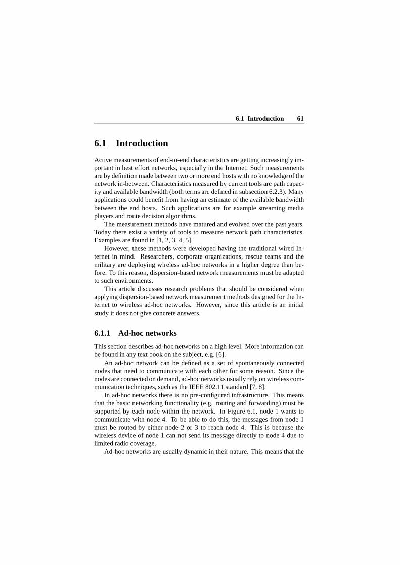
6.1 Introduction 61

6.1 Introduction

Active measurements of end-to-end characteristics are getting increasingly im-portant in best effort networks, especially in the Internet. Such measurementsare by definition made between two or more end hosts with no knowledge of thenetwork in-between. Characteristics measured by current tools are path capac-ity and available bandwidth (both terms are defined in subsection 6.2.3). Manyapplications could benefit from having an estimate of the available bandwidthbetween the end hosts. Such applications are for example streaming mediaplayers and route decision algorithms.

The measurement methods have matured and evolved over the past years.Today there exist a variety of tools to measure network path characteristics.Examples are found in [1, 2, 3, 4, 5].

However, these methods were developed having the traditional wired In-ternet in mind. Researchers, corporate organizations, rescue teams and themilitary are deploying wireless ad-hoc networks in a higherdegree than be-fore. To this reason, dispersion-based network measurements must be adaptedto such environments.

This article discusses research problems that should be considered whenapplying dispersion-based network measurement methods designed for the In-ternet to wireless ad-hoc networks. However, since this article is an initialstudy it does not give concrete answers.

6.1.1 Ad-hoc networks

This section describes ad-hoc networks on a high level. Moreinformation canbe found in any text book on the subject, e.g. [6].

An ad-hoc network can be defined as a set of spontaneously connectednodes that need to communicate with each other for some reason. Since thenodes are connected on demand, ad-hoc networks usually relyon wireless com-munication techniques, such as the IEEE 802.11 standard [7,8].

In ad-hoc networks there is no pre-configured infrastructure. This meansthat the basic networking functionality (e.g. routing and forwarding) must besupported by each node within the network. In Figure 6.1, node 1 wants tocommunicate with node 4. To be able to do this, the messages from node 1must be routed by either node 2 or 3 to reach node 4. This is because thewireless device of node 1 can not send its message directly tonode 4 due tolimited radio coverage.

Ad-hoc networks are usually dynamic in their nature. This means that the

62 Paper B

Node 1

Node 2

Node 3

Node 4

Figure 6.1: Wireless ad-hoc network with 4 nodes. Node 1 is sending a mes-sage to node 4 via node 3 since the radio in node 1 can not reach node 4’sposition.

nodes will move and thus the route used between two nodes willchange. Thereare several routing techniques for ad-hoc networks [6].

6.1.2 Dispersion-based measurements

Active end-to-end measurements of available bandwidth areusually dividedinto two phases; the data collection phase and the analysis phase.

In the data collection phase, a probe generator injects probe packets alongthe path to be measured. The probing scheme (i.e. the dispersion or separationbetween successive probe packets) is predefined by the sender. Two commonprobing schemes are the injection of probe packets in pairs or in a train, re-spectively [9, 10, 3, 11, 4]. The initial probe packet dispersion is proportionalto the probe rate.

The dispersion between successive probe packets changes when the probepackets traverse the network path. It either changes due to limited link capacityor due to interaction with other packets traversing the samepath (such packetsare called cross traffic). Limited link capacity will increase the dispersion be-tween probe packets while packet interactions may increaseas well as decreasethe dispersion.

The probe packets are received by a probe receiver. Upon reception, the

6.2 Research problems 63

probe packets are time stamped. Using these time stamps the probe packetdispersion at the receiver is calculated.

The second phase, the analysis, uses the dispersion values obtained fromthe data collection phase to produce an estimate. The difference between theinitial probe packet dispersion and the received probe packet dispersion is usedto produce an estimate of the path capacity or the available bandwidth.

The data collection and the analysis phases combined is called a measure-ment session.

6.2 Research problems

In this section we discuss properties of multiple-access networks that differfrom single-access networks. Multiple-access networks are for example basedon the 802.3 (Ethernet) or IEEE 802.11 (wireless) standards. In this article wefocus on wireless networks. In particular, we study IEEE 802.11b (hereaftercalled 802.11) wireless ad-hoc networks, which is one of thecommon stan-dards for radio communication. All topics are discussed from the perspectiveof dispersion-based probing schemes.

Dispersion-based probing schemes make implicit assumptions that the net-work properties, such as link capacity, cross traffic and theroute between endnodes are the same during the measurement (especially during the data collec-tion phase). However, dispersion-based measurements are not instantaneous.They run for some time period. Since wireless ad-hoc networks tend to be verydynamic, we must understand and compensate for the dynamic properties. Inthe following subsections we discuss how the link capacity may change due tocross traffic or due to node movement. We also address route changes, loss rateand time control issues.

6.2.1 Variable link capacity

In single-access networks, the link capacity on a link is determined by physi-cal characteristics of the link itself and is usually static. However, in 802.11bnetworks the link capacity is typically changing dynamically over time. Thisvariation is due to changing distance between nodes due to their mobility, ra-dio noise, weather conditions and physical obstacles. However, the link ratevariability is also due to cross traffic using the same radio frequency channelwithin the ad-hoc network.

64 Paper B

Below, we show simulation results that illustrate that the link capacity ischanging due to cross traffic. The simulation topology is shown in Figure 6.2and the simulation tool is ns-2 [12]. Two nodes generate cross traffic betweeneach other while the other two nodes are measuring network link characteristicsusing dispersion-based measurement methods.

Probe traffic

Cross traffic

Figure 6.2: A single hop wireless ad-hoc topology. Cross traffic and probepackets use the same shared medium. The cross traffic will be affecting thelink capacity.

The diagrams in Figure 6.3 show a comparison of the offered probe rateand the measured probe rate. The offered / measured ratio is shown on they-axis. The x-axis is the probe rate, starting at 1 Mbps. The measured proberate is based on the mean of the probe packet dispersion values obtained in thedata collection phase. The offered probe rate is predefined by the probe packetsender and hence known in advance.

The figure shows 4 diagrams corresponding to 4 different scenarios. Eachscenario uses the same topology, but the cross traffic vary. As long as theoffered probe rate and the measured probe rate quotient remains around 1, themean dispersion between successive probe packets are the same on the senderside and the receiver side. That is, we have an underload situation. When thecurve starts to rise the mean dispersion on the receiver side(i.e. the measuredvalue) is larger than on the sender side. This change in dispersion indicateswhere the available bandwidth is. The slope of the curve after this point isinversely proportional to the link capacity, according to TOPP [3].

In Figure 6.3 the cross traffic is, starting from the upper left diagram, 0


Mbps, 0.5 Mbps, 1 Mbps and 2 Mbps, respectively. The cross traffic is uni-formly distributed. The measured available bandwidth is 4.7 Mbps, 4.2 Mbps,3.2 Mbps and 2.8 Mbps, respectively. In this case the perceived link capac-ity is equal to the available bandwidth for each scenario. According to TOPP,the slope of the curves is inversely proportional to the minimum link capacityof the network path. The slopes of the curves are approximately 0.22, 0.28,0.33 and 0.38, respectively. Hence, for wireless networks the perceived linkcapacity will change due to cross traffic.

The ns-2 wireless simulation topology was configured to run at 11 Mbps.The probe packet size was 1500 bytes.

2 3 4 5 6 7 8 9 10

1

1.5

2

2.5

3

3.5

4

Probe rate (Mbps)

o/m

2 3 4 5 6 7 8 9 10

1

1.5

2

2.5

3

3.5

4

Probe rate (Mbps)

o/m

2 3 4 5 6 7 8 9 10

1

1.5

2

2.5

3

3.5

4

Probe rate (Mbps)

o/m

2 3 4 5 6 7 8 9 10

1

1.5

2

2.5

3

3.5

4

Probe rate (Mbps)

o/m

Figure 6.3: The offered probe rate is compared to the measured probe rate.The slope of each curve is inversely proportional to the linkcapacity. Thecross traffic rate is 0 Mbps in the upper left diagram, 0.5 Mbps, 1 Mbps and 2Mbps in the bottom right diagram.

Since active end-to-end measurement techniques measure the link charac-teristics during a time interval, the cross traffic load may change during thisinterval. If that happens, the link capacity might change during the measure-

66 Paper B

ment session. Measurement methods today do not address thisproblem. Sinceavailable bandwidth measurement methods rely on an estimate of the link ca-pacity, a changing link capacity will introduce errors in the available bandwidthestimation.

6.2.2 Moving nodes

In ad-hoc wireless networks the distance between mobile nodes may changedue to mobility. This creates problems that measurement methods must handle.

When two mobile nodes move away from each other the radio signal strengthwill go down. The link capacity will decrease in discrete steps when the radiosignal strength is reduced to certain threshold levels. That is, we have the sameproblem as in Section 6.2.1, where variable link capacity was discussed.

As described in the introduction, all routing in ad-hoc networks is done bythe nodes themselves. When nodes move around, the route between two nodesmay change since the signal strength may become zero betweentwo nodes inthe route. Hence, two or more different end-to-end routes may be measuredduring one single dispersion-based measurement session.

If a static network topology is assumed (which is what dispersion-basedmeasurement methods today typically do), this will cause problems. This topicis subject to further study. We will look into how to detect and handle routechanges when using dispersion-based measurement methods.

6.2.3 Loss rate

Packet losses are not very common in single-access networks, especially notin wired networks. When they arise it is typically due to queue overflow at arouter somewhere in the path. However, in 802.11b wireless networks the lossrate is much higher. This is due to collisions on the shared medium, corruptpackets, et cetera. Assume the following scenario. A dispersion-based mea-surement injects probe packets into the wireless network path. Its estimate ofthe available bandwidth becomesA. Using this rateA when sending pack-ets on the wireless link may cause packet losses due to the transmission errorproperties of the wireless medium. This means that the available bandwidth islimited not only by the packet dispersion (i.e. the packet rate) but also by theloss rate.

Because of this fact we propose a definition of the available bandwidth thataddresses this problem.


The link capacity is by definition the bit rate of the link (i.e. the number ofbits that can be transfered during time� ). Further, the path capacity is definedas the link capacity with the least bit rate on a given path consisting ofH links.It is defined asC = mini=1::H(Ci), wherei is the link index.

The utilization of a link is by definition the number of bits transfered duringtime � divided by the link capacity. The utilization is within the interval[0; 1℄.

The definition of available bandwidth on one single link is (link capacity) *(1 - utilization) during time� . The available bandwidth between two end hoststhen becomesA = mini=1::H(Ci � (1�ui)), whereui is the utilization of linki.

To compensate for the loss rate, a term describing the loss rate must beadded to the equation describing the available bandwidth above. We getA = [ mini=1::H(Ci � (1� ui))℄ � (1� Lpath); (6.1)

whereLpath describes the total probe packet loss rate due to contentionseenon the path when sending packets at a rate corresponding to the available band-width. Equation 6.1 assumes that all losses occur on or downstream the linkwith least available bandwidth. Should losses occur elsewhere, our definitionis conservative.

This definition also holds in ordinary single-access networks, since the lossrate is close to 0.

6.2.4 Time control

This subsection discusses the difference between single-access and 802.11 net-works at the MAC-layer. In 802.11 networks the sender at the application layerdoes not know when a packet is transmitted on the link. Packets that are sentfrom a node traverse the network protocol stack from the top layer down tothe lower layers. The top layers (application, transport and network layer) arethe same regardless if a single-access or a 802.11 network isused by the nodesending the packet. However, the lower layers (MAC and physical) differ.

When sending a packet using single-access networks we can approximatethe time between sending the packet from the application layer and transmittingthe packet onto the link. The time spent in the protocol stackis more or lessconstant for each packet, assuming that the send rate is not higher than thecapacity of the network itself. That is, we can calculate theoffered dispersionbetween two successive probe packets.

68 Paper B

Time

2) Busy channel, backoff and contention phase

3) Probe packet 4) ACK

1) Probe packet ready to be transmitted

5) Ready to send next probe packet

Figure 6.4: The MAC-layer scheme when sending a packet usinga 802.11network.

However, in a 802.11 wireless network the lower layers will induce timejitter between successive probe packets. This jitter depends on, among otherthings, cross traffic using the same radio frequency channel. In Figure 8.11the jitter effect is illustrated. A probe packet is sent in the application layerand traverses down through the protocol stack to the MAC layer. The probepacket is ready to be transmitted on the shared medium, indicated by (1) in thefigure. Because of other traffic the probe packet has to wait until the sharedmedium is idle. The time a probe packet is in the contention phase (shown by(2) in the figure) depends on the cross traffic. When the probe packet is actuallysuccessfully transmitted (3) the node has to wait until an acknowledgment isreceived (4). The time to receive an acknowledgment dependson other com-peting packets and the network latency. That is, the dispersion between twosuccessive probe packets is not deterministic.

When the analysis phase is performed, the offered dispersion values ob-tained from the data collection phase is one important component to produce agood estimate of the measured network path characteristic.Probe-packet dis-persion jitter will make the estimate of the network characteristic less accurate.To get more accurate estimates, the analysis requires more dispersion sampleswhich means that more probe packets have to be sent. However,this should beavoided since the bandwidth in wireless networks is usuallythe bottleneck.

Exactly how the dispersion jitter will affect current end-to-end dispersion-based measurement methods is a subject of further research.

6.3 Conclusions

In this paper we have analyzed properties in IEEE 802.11 ad-hoc networksthat differs from single-access networks, from the view of dispersion-basedmeasurement methods.

We have performed ns-2 simulations to show that the link capacity vary de-pending on the cross traffic load. Further, we have extended the term availablebandwidth to cope with packet losses in wireless networks. In the article weraised the thought that variable link capacity and loss ratemay cause problemsto dispersion-based measurement methods.

We have also discussed the problems of moving nodes, route changes anddispersion time jitter at the probe sender.

In future research, we intend to study how the link capacity vary in largernon-simulated topologies. Further we will study how to detect and handle routechanges in an ad-hoc network when using dispersion-based methods. Our ex-tended definition of available bandwidth is also subject of further study. Wewill investigate to what extent our extended definition is overly pessimistic. Fi-nally, we will explore how time jitter will affect contemporary available band-width measurement methods.

Bibliography

Bibliography

[1] Van Jacobson. Pathchar - a tool to infer characteristicsof Internet paths.Presented at the Mathematical Sciences Research Institute(MSRI), April1997. Slides available from ftp://ftp.ee.lbl.gov/pathchar/.

[2] Bruce Mah. pchar: A tool for measuring Internet path characteristics,June 2001. http://www.employees.org/~bmah/Software/pchar/.




[6] Charles Perkins. Ad hoc networking. Addison-Wesley, 2001.

[7] ISO/IEC. Ieee 802.11 standard. ieee standard for information technology.ISO/IEC 8802-11:1999(E), 1999.

[8] ISO/IEC. Corrigendum to ieee 802.11b standard 1999. ieee standard forinformation technology. ISO/IEC 8802-11:1999/Cor 1-2001(E), 2001.


70

[10] Constantinos Dovrolis, Parameswaran Ramanathan, andDavid Moore.What do packet dispersion techniques measure? InProceedings of IEEEINFOCOM, pages 905–914, Anchorage, AK, USA, April 2001.

[11] Ningning Hu and Peter Steenkiste. Evaluation and characterization ofavailable bandwidth probing techniques.IEEE Journal on Selected Areasin Communication, 2003.

[12] The network simulator - ns-2. http://www.isi.edu/nsman/ns/.

Chapter 7

Paper C:DietTopp: A firstimplementation andevaluation of a simplifiedbandwidth measurementmethod

Andreas Johnsson, Bob Melander and Mats BjorkmanIn proceedings to the Second Swedish National Computer Networking Work-shop (SNCNW), Karlstad, 2004

73

Abstract

This paper describes the active available bandwidth measurement tool Diet-Topp. It measures the available bandwidth and the link capacity on an end-to-end path having one bottleneck link. DietTopp is based on a simplified TOPPmethod. This paper describe and motivate the simplifications and assumptionsmade to TOPP. Further, the paper describes some of the DietTopp implemen-tation issues.

A first evaluation of DietTopp in a testbed scenario is made. Within thisevaluation the performance and measurement accuracy of DietTopp is com-pared to the state-of-the-art tools Pathload and Pathrate.

We show that DietTopp gives fast and accurate estimations ofboth theavailable bandwidth and the link capacity of the bottlenecklink.

7.1 Introduction 75

7.1 Introduction

Measurements in best-effort networks are important for network error diagno-sis and performance tuning but also as a part of the adaptive machinery of userapplications such as streaming video. Within our research we have focusedon actively measuring available bandwidth between two network end-points.Such active measurements are done by injecting probe packets (with a pre-defined separation) into the network. The probe packets are time stamped atthe receiver end. These time stamps are then used to form an estimate of theavailable bandwidth. This is discussed in more detail in Section 7.2.

State-of-the-art bandwidth measurement tools and methodsare for exampleTOPP [1], Pathload [2], Pathchirp [3], Delphi [4] and Spruce[5]. An overviewof methods and tools in this area can be found in [6].

Within the scope of this paper we have developed, implemented and eval-uated a new available bandwidth measurement tool called DietTopp. This toolrelies on a simplification of the TOPP bandwidth measurementmethod [1].We show that DietTopp gives fast and accurate estimates of both the availablebandwidth and the measured link capacity when there is one congested link inthe end-to-end path.

This paper is organized as follows. The TOPP measurement method isbriefly described in Section 7.2. The simplifications and assumptions made byDietTopp are discussed and motivated in Section 8.2.1. DietTopp implemen-tation issues are described in Section 7.4. Section 8.2.2 describes the testbedthat has been used to evaluate our DietTopp implementation,while Section 8.3shows and discusses the obtained results. Section 8.3 also compare DietToppto other state-of-the-art measurement tools.

7.2 TOPP: the original method

This section briefly describes the original TOPP measurement method that es-timates the available bandwidth and link capacity on an end-to-end path. Moreinformation on definitions and theory can be obtained from [1].

The TOPP measurement method is divided into two phases, the probingphase and the analysis phase. These two phases are separately described in thefollowing two subsections.

76 Paper C

7.2.1 Probe phase

Starting at some offered probe rateomin, the TOPP method injectsm probepacket trains, where each train containsk equally sized probe packets, into thenetwork path. When all probe trains corresponding to a proberateomin havebeen received on the other end, TOPP increases the offered rateo = omin+�o.Another set of probe packet trains are sent through the network at the new proberate. This is repeated until the offered probe rate reaches some specified proberateomax (i.e. o > omax).

The probe packet separation changes between the probe sender and theprobe receiver. This is due to thebottleneck spacing effect[7] which basicallysays that the time separation increases in a predictable manner when a link iscongested.

The receiver time stamps each packet arrival. Hence, the change in probepacket separation can be measured. The time stamps are then used to calculatethe measured probe ratem. When the measured probe rate and its correspond-ing offered probe rate is known the analysis phase of TOPP canbe executed.The analysis is described in the next subsection.

7.2.2 Analysis phase

The analysis builds on comparing the offered probe rateoi to the measuredprobe ratemi on each probe rate leveli. If plotting the ratiooi=mi on the y-axis andoi on the x-axis for alli, we get a plot like the theoretical one in Figure8.1. When the network is underloaded theoi=mi ratio will be close toy = 1.When TOPP increases the offered probe rate some link on the network path willeventually get saturated. Hence, the measured probe rate will decrease sincethe probe packet separation increases (due to the bottleneck spacing effect).This causes the curve to rise. Segmentb1 is linear and the slope corresponds tothe link bandwidth of the first congested link. The availablebandwidth of theend-to-end path is defined as the intersection ofy = 1 and the linear segmentb1 (t1).

If there are more than one congested link on the end-to-end path the curvewill be divided into several linear segments, when increasing the offered proberate. Each new segment,b2 andb3, corresponds to the fact that an additionallink has been congested. That is, the number of linear segments depends onthe number of saturated links on the end-to-end path. The saturation point foreach link can be calculated usingt1, t2 andt3 in the figure.

The original TOPP method can, in many cases, determine not only the end-

7.3 DietTopp 77

b

b

b

1

2

3

t tt1 2 3

Offe

red

/ Mea

sure

d pr

obe

rate

Offered probe rate

Figure 7.1: Plot of offered prob rate / measured probe rate asa function of theoffered probe rate. The three segmentsb1 - b3 corresponds to three congestedlinks while t1 - t3 are breakpoints between congested links.

to-end available bandwidth (corresponding to the intersection of y = 1 andthe linear segmentb1) but also the link available bandwidth of each congestedlink. This is done by extracting additional information from the linear segmentsshown in Figure 8.1. Exactly how this is done is described in [1].

7.2.3 TOPP complications

The problem with the original TOPP method is its complex iterative algorithmit uses to estimate the segment intersection points. This makes the TOPP anal-ysis phase computationally expensive. It is feasible, as shown in [1] but takesa lot of computation power.

7.3 DietTopp

This section describes DietTopp. That is, the simplifications we have made tothe TOPP analysis.

DietTopp assumes that only one link between the sender and the receiver iscongested. That is, there will only be one linear segment in Figure 8.1 (i.e.b1).Hence, the end-to-end link capacity is proportional to the slope of segmentb1and the end-to-end available bandwidth is defined as the intersection ofb1 andy = 1 (t1). That is, the iterative part of TOPP can be omitted.

78 Paper C

Since we want to identifyb1, the first step is to ensure that DietTopp sendsprobe packets at a rate above the available bandwidth (corresponding tot1 inFigure 8.1). This is done by calculating the proportional share,psmax, of theend-to-end path at probe rateomax. Hence,psmax = omax=(x + omax) � lwhereomax is the maximum offered probe rate,x the cross traffic andl thelink capacity of the congested link. Thepsmax is estimated by injecting a set ofprobe packets back-to-back into the network and then measure their separationat the receiver. Thepsmax is an overestimation of the available bandwidth, asdiscussed in [1] (and referred to as the asymptotic dispersion rate in [8]).

When DietTopp has obtained a value ofpsmax it continues the probingphase by injecting probe packets at rates in the interval[psmax; z � psmax℄,wherez is a constant. This will generateoi=mi values corresponding to thelinear segmentb1 in Figure 8.1. That is, DietTopp can calculate the link capac-ity by finding the slope ofb1 and the available bandwidth by calculating theintersection ofb1 andy = 1. This is done using linear regression.

We argue that the assumption that only one link is congested in a path is nottoo far fetched. Usually the bottlenecks are found in the access networks, closeto the user, for example when the user is using a wireless connection. Usuallywireless links provides a much lower bandwidth than the restof the links in thepath.

Other probing tools that assume one single bottleneck link are Spruce [5]and Delphi [4]. In addition, these tools require prior knowledge of the bottle-neck link capacity. This is not the case when using DietTopp.On the contrary,DietTopp will estimate that capacity as part of its estimation procedure.

7.4 Implementation of DietTopp

This section gives an overview of the DietTopp implementation. More infor-mation about the implementation ca be obtained by downloading the tool alongwith its source code [9].

DietTopp is designed for Unix system and is implemented in C++. It has asender and a receiver part. The senderprobesthe network path by injecting aset of packet trains at different rates similarly to TOPP (inthe original methodTOPP used pairs of probe packets instead of trains of probe packets). Thereceiver records the time for each probe packet arrival. These values are sentback to the probe sender for analysis. The analysis is done using our simplifiedTOPP method described in Sections 7.2 and 8.2.1.

The probe packets used by DietTopp are UDP/IP packets with a size of

7.5 The testbed 79

1500 bytes. The packets are divided in trains where each train consists of 16packets. On each probe rate level DietTopp sends 5 trains. DietTopp uses 15prob rate levels in the interval[psmax; z � psmax℄ by default.

When DietTopp is measuring the proportional share (described in Section8.2.1), 15 trains with 48 packets in each are sent at the maximum probe rate(i.e. the sender’s link speed).

The DietTopp implementation can be summarized as follows:

1. Send a set of probe trains at maximum rate

2. Record the probe packet arrival times at receiver

3. Send time stamps back to sender

4. The proportional share (ps) is estimated using the arrival times

5. The sender initiates and transmits a set of probe trains with rates in theinterval[1 � ps; 1:5 � ps℄

6. The receiver records the probe packet arrival times

7. The arrival times are sent back to the sender

8. The arrival times are analyzed using our simplified TOPP method

9. If the correlation is large enough and if the standard deviation smallenough DietTopp presents its results and terminates

10. Else, repeat from step 1, but increase the number of probepackets ineach train

7.5 The testbed

The testbed we have used in this work consists of 7 ordinary PCmachines. ThePCs acting as routers (R1 - R3) are connected by 10 Mbps links while the restof the links can communicate at 100 Mbps. The testbed is shownin Figure8.2. The probe tool sender is running onSwhile the receiver is running on thedestination machineD.

The cross traffic can either take the routeX1 ! R1 ! R2 ! X2 orthe routeX1 ! R2 ! R3 ! X2. The cross traffic itself is exponentiallydistributed and consists of 60, 148, 500 and 1500 byte packets (this corresponds

80 Paper C

S D

X1

X2

R1 R2 R3

Figure 7.2: The testbed used for a first evaluation of DietTopp.

to the packet size at thelink layer). This distribution of packet sizes originatesfrom findings in [10]. The cross traffic is generated bytg [11].

An important observation is that the ethernet cards used in the testbed cannot send packets back-to-back. The cards add a gap corresponding to 25 bytesbetween two successive packets. This will be manifested as if all packets willhave an increased effective packet size. That is, a 500 byte packet will havean effective packet size of 525 byte when the ethernet card continuously has toforward packets.

7.6 DietTopp Evaluation

This section presents a first evaluation of DietTopp. We haveperformed mea-surements in the testbed described in Section 8.2.2. The cross traffic flowsthrough the routeX1! R1! R2! X2. That is, the probe packets injectedby DietTopp are only affected by cross traffic on one hop (i.e.between onepair or routers). The cross traffic composition and distribution is described inSection 8.2.2.

We have used the state-of-the-art tools Pathload and Pathrate [2, 12] tocompare the accuracy and performance of the measured available bandwidthand link capacity. We show that DietTopp gives accurate and fast estimates.The results are presented and discussed in the following subsection.

7.6.1 Measurement results

The measurements in Figure 8.3 originate from DietTopp measurements underfour different cross traffic intensities - 0, 3.75, 6.26 and 8.76 Mbps (shown

7.6 DietTopp Evaluation 81

on the x-axis). The y-axis shows the measured link capacity (thick solid line)and measured available bandwidth (thin solid line). The link capacity has adecreasing trend when increasing the cross traffic intensity. Exactly why thishappens is subject of further research.

Figure 7.3: Link capacity (thick solid line) and available bandwidth (thin solidline) measured by DietTopp.

Figure 7.4: Link capacity measured by DietTopp (solid line)and Pathrate(dashed line).

The diagram in Figure 8.4 compares the measured link capacity when usingDietTopp (solid line) and Pathrate (dashed line). It is clear that DietTopp un-derestimates the link capacity in comparison to Pathrates estimation. However,Pathrates estimation is in turn an underestimation compared to the theoretical

82 Paper C

link capacity of 10 Mbps.

Figure 7.5: Available bandwidth measured by DietTopp (solid line) andPathload (dashed line). The theoretical available bandwidth is shown as thedouble dot dashed line.

Figure 7.6: Time consumption at different cross traffic rates. The solid linecorresponds to DietTopp while the dashed line corresponds to Pathload.

The diagram in Figure 8.6 is a comparison of the measured available band-width. The solid line corresponds to DietTopp while the dashed line corre-sponds to Pathload. The double dot dashed line is the theoretical availablebandwidth under different cross traffic rates. Here we see that both methodsestimate the available bandwidth quite well, even if Pathload tends to overesti-mate in some cases.

7.6 DietTopp Evaluation 83

The diagram in Figure 8.5 is a performance comparison of DietTopp andPathload. The diagram compares the time consumption of DietTopp (solid line)and Pathload (dashed line). As can be seen, the time to measure the availablebandwidth using DietTopp is almost constant while for Pathload the time growsexponentially.

Figure 7.7: Number of transfered bits by DietTopp (solid line) and Pathload(dashed line).

Figure 7.8: Number of transferred bits / second by DietTopp (solid line) andPathload (dashed line).

It should also be noted that DietTopp does not only measure the availablebandwidth during its execution time, but also the link capacity of the congestedlink.

The diagrams in Figure 8.7 and 8.8 compare the number of bits transferredtotally during a measurement session and the number of bits transferred persecond when using DietTopp (solid line) and Pathload (dashed line). Pathloaduses more bits, but since DietTopp runs over a shorter periodof time DietToppis more aggressive as can be seen in the diagram in Figure 8.8.

To summarize, our first evaluation of DietTopp shows that DietTopp esti-mates both the link capacity and the available bandwidth with comparable andin some cases better accuracy than Pathload and Pathrate. Further, our toolruns over a shorter period of time. The drawback is that DietTopp is moreaggressive than both Pathload and Pathrate.

In our continued work we will investigate how the aggressiveness of Diet-Topp affects TCP flows and other communication protocols. Wewill also try tomake estimations of the available bandwidth and the link capacity with equalaccuracy but with fewer probe packets.

7.7 Conclusions

We have simplified the TOPP measurement method and implemented the newmethod in a tool that we call DietTopp. We have described and motivatedthe simplifications and assumptions made to TOPP. Further, we have done aninitial evaluation of the accuracy and performance of DietTopp. We have alsocompared DietTopp to the measurement tools Pathload and Pathrate.

We have shown that our tool gives accurate estimate, in the one hop case,of the available bandwidth and an acceptable estimate of thelink capacity.Compared to Pathload our solution is quicker, but with the drawback of a highernetwork aggressiveness.

We will continue our research by investigate how DietTopp reacts whencross traffic is present on multiple links. We will try to find away to keep theestimation accuracy but decrease the number of probe packets sent. Finally, wewill investigate how the accuracy and speed is affected by wireless networks.

Bibliography




[4] Vinay Ribeiro, Mark Coates, Rudolf Riedi, Shriram Sarvotham, BrentHendricks, and Richard Baraniuk. Multifractal cross-traffic estimation.In Proceedings of ITC Specialist Seminar on IP Traffic Measurement,Modeling and Management, Monterey, CA, USA, September 2000.


[6] R.S. Prasad, M. Murray, C. Dovrolis, and K. Claffy. Bandwidth estima-tion: metrics, measurement techniques, and tools. IEEE Network Maga-zine, 2003.


85


[9] Andreas Johnsson. Diettopp implementation, beta version.http://www.idt.mdh.se/ajn12/.


[11] Paul E. McKenney, Dan Y. Lee, and Barbara A. Denny. Traffic generatorsoftware release notes. SRI International and USC/ISI Postel Center forExperimental Networking, January 2002.

[12] Manish Jain and Constantinos Dovrolis. Pathload: a measurement toolfor end-to-end available bandwidth. InPassive and Active Measurement(PAM) Workshop 2002 Proceedings, pages 14–25, Ft Collins, Co, USA,March 2002.

Chapter 8

Paper D:Bandwidth Measurement inWireless Networks

Andreas Johnsson, Bob Melander and Mats BjorkmanSubmitted for publication

87

Abstract

For active, probing-based bandwidth measurements performed on top of theunifying IP layer, it may seem reasonable to expect the measurement problemin wireless networks, such as ad-hoc networks, to be no different than the onein wired networks. However, in networks with 802.11 wireless links we showthat this is not the case. We also discuss the underlying reasons for the observeddifferences.

Our experiments show that the measured available bandwidthis dependenton the probe packet size (contrary to what is observed in wired networks). An-other equally important finding is that the measured link capacity is dependenton the probe packet sizeandon the cross-traffic intensity.

The study we present has been performed using a bandwidth measurementtool, DietTopp, that is based on the previously not implemented TOPP method.DietTopp measures the end-to-end available bandwidth of a network path alongwith the capacity of the congested link.

8.1 Introduction 89

8.1 Introduction

Wireless networks, used when connecting to the Internet or when several nodeswant to communicate in an ad-hoc manner, are becoming more and more pop-ular. Because of the increased dependence on wireless network technology, itis important to ensure that methods and tools for network performance mea-surement also perform well in wireless environments. In this paper, we focuson performance measurements in terms of network bandwidth,both link band-width and the unused portion thereof; the available bandwidth.

Measurement of network properties such as available bandwidth in for ex-ample ad-hoc networks are important for network error diagnosis and perfor-mance tuning but also as a part of the adaptive machinery of network applica-tions such as streaming audio and video. Since the exact route between twonodes in an ad-hoc network is usually unknown and may change without no-tification to the application layer the end-to-end measurement of the availablebandwidth should not require any infrastructure or pre-installed components oneach node. To achieve that, intermediate end-to-end bandwidth measurementmethods can be applied.

State-of-the-art bandwidth measurement methods are for example Pathchirp[1], Pathload [2], Spruce [3] and TOPP [4]. The basic principle is to inject aset of measurement packets, so calledprobe packets, into the network. Theprobe packets traverse the network path to a receiver node, which time stampseach incoming probe packet. By analyzing these time stamps estimates of thelink capacity and/or the available bandwidth can be made. For many end-to-end available bandwidth measurement methods no previous knowledge ofthe underlying network topology is needed. Therefore, bandwidth estimationmethods are well suited for end-to-end performance measurements in ad-hocnetworks.

The existing methods differ in how probe packet are sent (theflight pat-terns) and in the estimation algorithms used. An overview ofmethods andtools in this area can be found in [5].

In the following sections, we describe and measure bandwidth estimationcharacteristics when probing in 802.11 wireless networks.We show that boththe measured available bandwidth and the measured link capacity are depen-dent on the probe packet size. Furthermore, our measurements indicate that themeasured link capacity is also dependent on the cross-traffic rate. We discussthe origins of some of the observed behavior.

The measurements have been performed in a testbed containing both wire-less and wired hops. Our testbed topology only consist of onewireless hop,

90 Paper D

but we believe that our results illustrate the measurement problem for largerad-hoc networks, consisting of several wireless hops, as well. To produce mea-surement results we have used DietTopp, a tool that measuresthe availablebandwidth and link capacity of an end-to-end path. For comparisons and toillustrate that our observations are not tied to a certain measurement tool, wehave also used the tool Pathload, that measure the availablebandwidth of anend-to-end path, in our experiments.

Earlier work has touched upon the problem of active measurements ofbandwidth in wireless networks. In [6] we discuss the main problem areaswhen deploying existing bandwidth measurement methods in ad-hoc networks.For example, we observed using ns-2 simulations, that the measured link ca-pacity show dependence on the cross-traffic rate.

Measurement results presented in [7] indicate that the available bandwidthis dependent of the probe packet size. Our study extends thatstudy by showingthat both the available bandwidth and the measured link capacity depend onboth the probe packet size and the cross-traffic rate. Further, we use a morecomplex measurement topology to verify their findings.

The rest of this paper is organized as follows. Section 8.2.1describes theoriginal TOPP measurement method. DietTopp, which is our implementationof a modified TOPP method, is also presented. Section 8.2.2 isa description ofthe testbed we have used for the investigation of the bandwidth measurementproblem in wireless networks. Section 8.3 shows measurement results fromusing DietTopp in wired as well as in wireless networks. We discuss the re-sults and compare them to results obtained by Pathload. In section 8.4 someimportant observations are made. The paper ends with conclusions in section8.5.

8.2 Experimental setup

This section describes our experimental setup. That is, themeasurement tool(DietTopp), our testbed and what kind of measurements we have performedand their relevance to ad-hoc networks.

8.2.1 DietTopp

DietTopp has its origins in the previously not implemented TOPP [4] methodand uses the measured dispersion of probe packet trains to calculate bandwidthestimates.

8.2 Experimental setup 91

In short summary DietTopp works as follows. Starting at someofferedprobe rateomin, DietTopp injectsm probe packet trains, where each train con-tainsk equally sized probe packets, into the network path. When allprobetrains corresponding to a probe rateomin have been transmitted, DietTopp in-creases the offered rateo by �o. Another set of probe packet trains are sentinto the network with the new probe rate. This is repeatedi times until theoffered probe rate reaches some specified probe rateomax.

y = 1

oi

oi

/m

i

a

b

Figure 8.1: Plot of the ratiooi=mi as a function ofoi.The probe packet dispersion may change as the probe packets traverse the

network path between the probe sender and the probe receiver. This is due tothebottleneck spacing effect[8] and/or interactions with competing traffic.

The receiver time stamps each probe packet arrival. Hence, any change inprobe packet separation can be measured. The time stamps areused to calculatethe measured probe ratemi.

When all measurements are collected, DietTopp computes theratio oi=mifor all i. If plotting the ratiooi=mi on the y-axis andoi on the x-axis forall i, we get a plot like the theoretical one in Figure 8.1. If the dispersionof the probe packets would remain unchanged after traversalof the networkpath, the measured rates,mi, on the receiver side would be the same as theoffered ratesoi. Expressed differently, the ratiooi=mi would equal 1. The linkthat limits the available bandwidth of the path will eventually get congestedwhen increasing the offered probe rate. This causes the curve to rise sincethe ratem does not increase as much as the rateo. If the link capacity island the available bandwidth isa the relation betweenoi andmi is given byo=m = (1� a=l) + o=l (when one link is congested) [4].

92 Paper D

Segmentb in the figure is linear and the slope corresponds to the link ca-pacity of the congested link. The available bandwidth of theend-to-end path isdefined as the intersection ofy = 1 andb (i.e. a in the figure) [4].

To speed up the probing phase of DietTopp we want to avoid measurementsbelowa. That is, we want to ensure thatomin > a. This is done by estimatingmmax which is done by injecting a set of probe packets at rateomax and thenmeasure their separation at the receiver. According to [4]mmax is greater thanthe available bandwidth (mmax is referred to as the asymptotic dispersion ratein [9]).

Having a value ofomin > a, the procedure described above is executed tofind the link capacity and available bandwidth.

DietTopp is implemented in C++ on Unix platforms and can be downloadedfrom [10].

8.2.2 The testbed

The testbed used consists of 9 computers running Linux, shown in Figure 8.2.The link speed for each link is shown in the figure. The links betweenXw1,Xw2 andR1 are 802.11b wireless links while the link betweenS andR1 caneither be a 802.11b wireless link or a 100 Mbps wired link.

S

D

X1

X2

R1 R2 R3

Xw2

Xw1

10/100 10/100 100Mbps

100Mbps

100Mbps

100Mbps

100Mbps

11/100Mbps

11Mbps

11Mbps

Figure 8.2: The testbed is constructed by one wireless link,three routers andseveral cross-traffic generators (on both the wireless and the wired links)

The cross traffic, generated by a modified version oftg [11], can either takethe routeX1 ! R1 ! R2 ! X2 or the routeX1 ! R2 ! R3 ! X2.Cross traffic can also be generated byXw1andXw2on the wireless hop. Thecross traffic is either constant bit rate (CBR), exponentialor pareto distributed(shape = 1.5). Further, the cross traffic consists of 60 (46%), 148 (11%), 500(11%) and 1500 (32%) byte packets. This distribution of packet sizes originatesfrom findings in [12].

8.3 Experimental results 93

8.2.3 Experiments

In this paper we want to identify possible problems associated with bandwidthmeasurements in wireless networks, such as ad-hoc networks. First we showtwo measurements using DietTopp in a wired scenario. This isto validate thatour tool is sound in the simple wired case before turning attention to the morecomplex case of estimating end-to-end bandwidth in wireless networks. Wecompare DietTopp results to theoretical values as well as tovalues obtainedfrom Pathload.

The measurements in the wireless scenario is done using DietTopp. Weelaborate on the impact of probe packet size, the cross-traffic distribution,the number of probe packets sent and on the number of cross-traffic genera-tors in the wireless network. We compare our results to results obtained fromPathload.

This work is related to the work presented in [7]. We extend and com-plement that work in the following way: We use our newly developed toolDietTopp, that measured both the link capacity and the available bandwidth ofthe bottleneck link. Previous work has only focused on the available bandwidthon wireless links. Further, we use a more complex testbed topology.

8.3 Experimental results

This section presents the results obtained using DietTopp in wired and wirelessscenarios. We have used Pathload [2] to compare and discuss the obtainedmeasurement results. In the diagrams all measurement results are shown witha 95% confidence interval.

8.3.1 Measurement results in wired networks

This section presents measurements done with both DietToppand Pathloadin an all wired scenario. This section is to show by example that our tool,DietTopp, measures both the link capacity and the availablebandwidth in asound way.

The diagram in Figure 8.3 illustrates results from DietToppmeasurementsusing four different cross traffic intensities on link R1 - R2(10 Mbps linkcapacity in this case), shown on the x-axis. The cross trafficat link R2 - R3(100 Mbps link capacity) is a 8.76 Mbps stream. Both cross-traffic streams areexponentially distributed. The y-axis shows the measured link capacity (thinsolid line), the measured available bandwidth (thin dashedline), the theoretical

94 Paper D

link capacity (thick solid line) and the theoretical available bandwidth (thickdashed line). As can be seen the correlation between measurement results andthe theoretical values is good.

Figure 8.3: Link capacity (solid lines) and available bandwidth (dashed lines).Thick lines corresponds to theoretical values while thin lines are values ob-tained from DietTopp.

The diagram in Figure 8.4 is a comparison of the measured available band-width using DietTopp (dashed line) and Pathload (solid line). The same testbedand cross traffic setup is used as in Figure 8.3. We see that both tools reportsimilar estimates of the available bandwidth.

We have now given an indication that DietTopp estimates boththe link ca-pacity as well as the available bandwidth in wired network with good accuracy,both compared to theoretical values and compared to one state-of-the-art band-width measurement tool, Pathload. In the next subsection weinvestigate theimpact of wireless bottlenecks on the measurement results.

8.3.2 Measurement results in wireless networks

This subsection presents our results from measurements using DietTopp wherethe bottleneck is a wireless link (the link between S and R1 inthe testbed asdescribed in subsection 8.2.2) which is the case in ad-hoc wireless networks.Cross traffic is present on both of the wired links R1 - R2 and R2- R3, butthe rate is limited to approximately 9% of the correspondinglink capacity (100Mbps in this case). That is, the wireless link is the link thatlimits both the linkcapacity and the available bandwidth. The cross traffic at the 100 Mbps links


Figure 8.4: Available bandwidth measured by DietTopp (dashed line) andPathload (solid line).

between R1, R2 and R3 is pareto distributed and consists of 4 different packetsizes. The cross-traffic configuration on the wired links is the same for eachexperiment presented in this section.

The probe packet size affects both the measured link capacity and the avail-able bandwidth estimate when the bottleneck in an end-to-end path is a wirelesslink. We illustrate and describe this phenomenon in a set of diagrams below.

Figure 8.5: Available bandwidth (dashed lines) and measured link capacity(solid lines) measured under 0, 250 Kbps and 500 Kbps cross-traffic rates).

The two upper curves in Figure 8.5 show the measured link capacity (solidline) and the measured available bandwidth (dashed line) when no cross traffic

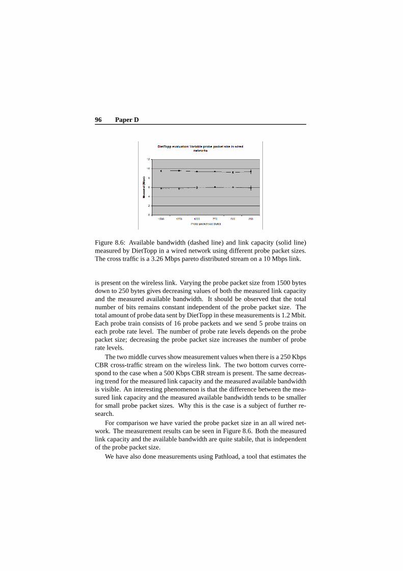
96 Paper D

Figure 8.6: Available bandwidth (dashed line) and link capacity (solid line)measured by DietTopp in a wired network using different probe packet sizes.The cross traffic is a 3.26 Mbps pareto distributed stream on a10 Mbps link.

is present on the wireless link. Varying the probe packet size from 1500 bytesdown to 250 bytes gives decreasing values of both the measured link capacityand the measured available bandwidth. It should be observedthat the totalnumber of bits remains constant independent of the probe packet size. Thetotal amount of probe data sent by DietTopp in these measurements is 1.2 Mbit.Each probe train consists of 16 probe packets and we send 5 probe trains oneach probe rate level. The number of probe rate levels depends on the probepacket size; decreasing the probe packet size increases thenumber of proberate levels.

The two middle curves show measurement values when there is a250 KbpsCBR cross-traffic stream on the wireless link. The two bottomcurves corre-spond to the case when a 500 Kbps CBR stream is present. The same decreas-ing trend for the measured link capacity and the measured available bandwidthis visible. An interesting phenomenon is that the difference between the mea-sured link capacity and the measured available bandwidth tends to be smallerfor small probe packet sizes. Why this is the case is a subjectof further re-search.

For comparison we have varied the probe packet size in an all wired net-work. The measurement results can be seen in Figure 8.6. Boththe measuredlink capacity and the available bandwidth are quite stabile, that is independentof the probe packet size.

We have also done measurements using Pathload, a tool that estimates the


available bandwidth using 300 byte packets. The results obtained from usingPathload in our testbed with different cross-traffic distributions and intensitiescan be seen in Table 8.1. When comparing results obtained by Pathload (inFigure 8.5) to those of DietTopp we can see that Pathload reports availablebandwidth measurement estimations that are in line with estimations made byDietTopp (using interpolation between packet sizes 250 and500 bytes).

Cross traffic Measurement (Mbps)

0 2.32 - 2.39250k cbr 1.67 - 1.67250k exp 1.73 - 1.73250k par 1.40 - 1.63500k cbr 0.96 - 0.99500k exp 0.87 - 0.95500k par 1.27 - 1.29

Table 8.1: Measurement results obtained from Pathload under the influence ofdifferent cross-traffic distributions.

Figure 8.7: Available bandwidth (dashed lines) and measured link capacity(solid lines) measured under 0, 250 Kbps and 500 Kbps exponentially dis-tributed coss-traffic.

Figures 8.7 and 8.8 report results from the same type of measurements asin Figure 8.5. However, in these two scenarios we have used more complexcross-traffic distributions. In Figure 8.7 we have used exponentially distributed

98 Paper D

Figure 8.8: Available bandwidth (dashed lines) and measured link capacity(solid lines) measured under 0, 250 Kbps and 500 Kbps pareto distributedcross-traffic.

arrival times for the cross-traffic packets while in Figure 8.8 we have usedpareto distributed arrival times. As can be seen in both figures the confidenceintervals are larger when the cross traffic is burstier. It isalso obvious that thecurves are less smooth compared to the CBR case in Figure 8.5.In the paretocase (Figure 8.8) it is hard to distinguish between the 250 Kbps and 500 Kbpsmeasurements of link capacity and available bandwidth. However, we can stillsee that the measured link capacity and available bandwidthis dependent onboth the probe packet size and the cross-traffic rate. Again,comparing themeasurement results (at the 300 byte probe packet size level) with results ob-tained by Pathload (in Table 8.1) we can conclude that the available bandwidthestimate characteristics are compatible.

In Figure 8.9 we vary the probe packet size in the same manner as above.However, instead of keeping the total number of bits transfered constant wekeep the number of probe packets sent constant. The cross traffic is paretodistributed. We see that even though the total amount of probe data sent is lessat each probe packet size level the confidence intervals remain low.

In Figure 8.10 two cross-traffic generators are generating 250 Kbps of CBRcross traffic each. Comparing Figure 8.10 to the measurementresults in Figure8.5 we see that the confidence intervals are larger when having multiple cross-traffic generators.


Figure 8.9: Available bandwidth (dashed lines) and measured link capacity(solid lines) measured under 0 and 500 Kbps pareto distributed cross-traffic.The number of probe packets is constant.

8.3.3 Wireless measurement results discussed

In this subsection we will discuss the results obtained in the previous sub-section and the reasons for the difference between DietToppmeasurements inwired and in wireless networks.

We will derive the differences from Figure 8.11 which illustrates the proce-dure for sending a packet in a 802.11 wireless network. First, the radio trans-mitter at the wireless node needs a clear channel to send its packet on. This isillustrated by step 1 and 2 in the figure. If someone else is using the channelthe sender does a back-off. It tries again after some time. Eventually the packetis sent, step 3 in the figure. When the receiving node gets the whole packet itresponds with a link-layer acknowledgment to the sender (step 4). The sendercan now transmit the next packet.

The reason for the decreasing measurement of the measured available band-width can be traced to the link-level acknowledgments in step 3 and 4 in thefigure. That is, if the probe packet is small, the overhead induced by the link-level acknowledgment is larger than if the probe packet werelarge. We cometo the conclusion that large probe packets will measure a larger available band-width than small probe packets.

The contention phase (step 1 and 2 in the figure) is independent of thepacket size. The contention phase is instead dependent on the number of send-ing nodes in the wireless networks. Increasing the number ofstations that wantto send traffic over the wireless network increases the waiting time for each

100 Paper D

Figure 8.10: Available bandwidth (dashed lines) and measured link capacity(solid lines) measured under 0 and 500 Kbps CBR cross-traffic. The crosstraffic is generated by two different sources (250 Kbps each).

Time

2) Busy channel, backoff and contention phase

3) Probe packet 4) ACK

1) Probe packet ready to be transmitted

5) Ready to send next probe packet

Figure 8.11: A schematic picture of the procedure for sending a packet in a802.11 wireless network.

node. It also increases the variance of the waiting time.In Figure 8.10 two cross-traffic generators are generating 250 Kbps of CBR

cross traffic each as described above. Since we have two wireless nodes send-ing traffic, this is likely to affect the contention phase in Figure 8.11 in such away that we get larger confidence intervals in our measurement results. Com-paring Figure 8.10 to the measurement results in Figure 8.5 we indeed see thatthe confidence intervals are larger when having multiple cross-traffic genera-tors.

The results concerning the available bandwidth are in line with results dis-cussed in [7]. We validate and extend those findings by using more complextestbed scenarios and our own tool DietTopp.

A theoretical description of why the measured link capacityis dependent

8.4 Other observations 101

on both the probe packet size and the cross-traffic intensityis a subject of futureresearch.

A final remark is that in most figures we can see that the confidence inter-vals decrease with the probe packet size. Hence, we can draw the conclusionthat we get values with low standard deviation with small probe packets. How-ever, why this is the case is also a subject of future research.

8.4 Other observations

Due to the fact that the probe packet size affects both the measured link ca-pacity and the measured available bandwidth when using DietTopp, a possiblemethod to identify a wireless bottleneck link in a network path could be: ifthe available bandwidth (and the measured link capacity) changes when prob-ing the path with different packet sizes, this can be taken asan indication thatthe path includes a wireless bottleneck. This is important since, as we havediscussed, wireless bottlenecks have different characteristics than wired bottle-necks. This is also interesting from an semi-ad-hoc perspective: when one nodeof an ad-hoc network is connected to an infrastructure, suchas the Internet, itis important to determine whether the bottleneck is within the ad-hoc networkor within the infrastructure. Is the bottleneck within the ad-hoc network theremight be possibilities to route the data differently. Also,ad-hoc router proto-cols can perform better with an understanding of bottlenecks within the ad-hocnetwork. However, this subject is left to future research.

An important consequence of the measurements we have presented in thispaper is that the available bandwidth will be application dependent in ad-hocnetworks and when wireless links are a bottleneck in general. For example, avoice over IP application or a distributed game probably usesmall packets tosend data while a file transfer application may use larger packets. The availablebandwidth for the applications will not be the same due to their packet size dis-tribution, as indicated by the figures above that show decreasing measurementvalues when decreasing the probe packet size. This means that when probing apath containing a wireless bottleneck link the estimation tool must use a probepacket size distribution that corresponds to the specific application.

8.5 Conclusion

In this paper we have shown measurements that illustrate thedifference be-tween bandwidth measurements in wired and wireless networks, such as ad-

102 Paper D

hoc networks. We have discussed some of the underlying reasons for thesedifferences while other reasons are left to further research. We have used ourown tool, DietTopp, to produce measurement results throughout the paper. Forcomparison and validity we have used Pathload. The measurements have beenperformed in a testbed where we have used different kinds of cross traffic, fromsimple CBR to bursty pareto distributed cross traffic.

Our conclusions are that measurements in wireless networksare associatedwith difficulties that can result in misleading bandwidth estimations. We haveshown that the packet size is critical to the bandwidth measurement value ofboth the link capacity and the available bandwidth. Further, we have shownthat the measured link capacity on wireless links does not only depend on thepacket size, but also on the cross traffic intensity. We have also addressed theproblem of application dependent probing.

Future research is to investigate why small packets gives a lower variancewhen used for active probing in wireless networks. We will also investigatewhy the measured link capacity vary when the probe packet size vary. It is alsoimportant to study what the variable measured link capacityobtained meansfor wireless network applications.

Bibliography





[5] R.S. Prasad, M. Murray, C. Dovrolis, and K. Claffy. Bandwidth estima-tion: metrics, measurement techniques, and tools. IEEE Network Maga-zine, 2003.

[6] Andreas Johnsson, Mats Bjrkman, and Bob Melander. A study ofdispersion-based measurement methods in ieee 802.11 ad-hoc networks.In Proceedings of the International Conference on Communication inComputing, Las Vegas, 2004.

[7] Karthik Lakshminarayanan, Venkata N. Padmanabhan, andJitendra Pad-hye. Bandwidth estimation in broadband access networks. InIn Proceed-ings to the Internet Measurement Conference, 2004.

103



[10] Andreas Johnsson. Diettopp implementation, beta version.http://www.idt.mdh.se/ajn12/.

[11] Paul E. McKenney, Dan Y. Lee, and Barbara A. Denny. Traffic generatorsoftware release notes. SRI International and USC/ISI Postel Center forExperimental Networking, January 2002.


bandwidth measurements in wired and wireless networks - idt - mrtc

Documents