1

Capacity Bounds and Degrees of Freedom forMIMO Antennas Constrained by Q-Factor

Casimir Ehrenborg, Member, IEEE, Mats Gustafsson, Senior Member, IEEE,and Miloslav Capek, Senior Member, IEEE

Abstract—The optimal spectral efficiency and number ofindependent channels for MIMO antennas in isotropic multipathchannels are investigated when bandwidth requirements areplaced on the antenna. By posing the problem as a convexoptimization problem restricted by the port Q-factor a semi-analytical expression is formed for its solution. The antennas aresimulated by method of moments and the solution is formulatedboth for structures fed by discrete ports, as well as for designregions characterized by an equivalent current. It is shown thatthe solution is solely dependent on the eigenvalues of the so-called energy modes of the antenna. The magnitude of theseeigenvalues is analyzed for a linear dipole array as well as aplate with embedded antenna regions. The energy modes are alsocompared to the characteristic modes to validate characteristicmodes as a design strategy for MIMO antennas. The antennaperformance is illustrated through spectral efficiency over the Q-factor, a quantity that is connected to the capacity. It is proposedthat the number of energy modes below a given Q-factor can beused to estimate the degrees of freedom for that Q-factor.

Index Terms—MIMO communication, degrees of freedom,computational electromagnetics, optimization, eigenvalues andeigenfunctions, antenna theory.

I. INTRODUCTION

MODERN communication systems often make use ofmultiple-input-multiple-output (MIMO) antennas. They

utilize spatial multiplexing to dramatically increase the trans-mitted bit-rate, or capacity, in comparison to single antennasystems [4], [5]. The optimal performance of MIMO systemsis therefore a topic of great interest. Many different methodshave been developed to evaluate maximum capacity underdifferent conditions and assumptions. For example by con-sidering spherical regions [6], [7], or treating the problemthrough an information theoretical approach [8], [9], [10],[11], [12]. In [13], [14] the authors presented a novel methodfor calculating optimal spectral efficiency of arbitrary antennadesigns using convex current optimization.

Manuscript received November 10, 2021. This work was supported by theSwedish foundation for strategic research (SSF) under the program appliedmathematics and the project Complex analysis and convex optimization forelectromagnetic design and by the Czech Science Foundation under Project19-06049S.

C. Ehrenborg is with the Department of Electrical Engineering, KU Leuven,Kasteelpark Arenberg 10 postbus 2440, 3001 Leuven, Belgium. (E-mail:casimir.ehrenborg@kuleuven.be).

M. Gustafsson is with the Department of Electrical and InformationTechnology, Lund University, Box 118, SE-221 00 Lund, Sweden. (Email:mats.gustafsson@eit.lth.se).

M. Capek is with the Department of Electromagnetic Field, Faculty ofElectrical Engineering, Czech Technical University in Prague, 166 27 Prague,Czech Republic (E-mail: miloslav.capek@fel.cvut.cz).

Design of MIMO antennas is based on effectively excitingdiscrete communication channels with low correlation [4]. Aproposed strategy for accomplishing this is to design the an-tennas such that they effectively excite modes with orthogonalradiation patterns, such as characteristic modes [15], [16], [17],[18]. A modal analysis method for analyzing MIMO antennasdesign, constrained by radiation efficiency, was presentedin [14]. This method is based on analyzing the eigenvaluesof a set of modes known as radiation modes to predict theperformance of a MIMO antenna. However, one of the openquestions of this technique is if it can be generalized to otherconstraining parameters, such as bandwidth.

Electrically small antennas suffer from a degradation inpossible performance as their size is reduced compared to thewavelength. Some of the parameters where this is most evidentare radiation efficiency, directivity, and bandwidth [19], [20],[21], [22]. Bandwidth can be estimated, for electrically smallsystems, through the Q-factor defined as the quotient ofenergy stored in a system over power dissipated by it [23].This relation accurately estimates the bandwidth, for singlefeed, single resonance systems [1], however, it does not holdfor multi-port systems. In this paper, this is addressed byconsidering a multi-port system as a superposition of singleport systems. Each port has a well defined Q-factor calculatedfrom the stored energy of the current induced by that port [24].These port currents make up the total current distribution onthe antenna when added together. The Q-factor of the totalcurrent is therefore an implicit indication of the Q-factor ineach port. In this way, restricting the Q-factor of the totalcurrent density implicitly imposes a bandwidth requirementon the system.

In this paper optimal spectral efficiency is calculated usingthe method from [14] for MIMO antennas transmitting in auniform multipath environment restricted by a required Q-factor. The optimization problem is formulated in the sourcesof the antenna design problem, either the feeding voltage ofa fixed antenna array, or the current distribution in a designregion. These two cases are studied to gain different insightsinto how to maximize spectral efficiency.

The antenna array is optimized by recasting the optimizationproblem in the port voltages. This is used to study theplacement of canonical dipole antennas to gain an intuition formaximizing spectral efficiency. An advantage of this approachis the feasibility of the bound via direct realization of the portvoltage excitation proposed by the optimization routine. Thecurrent optimization problem is solved for a few sub-regionsembedded in a plate. The performance and placement of these

arX

iv:1

905.

0310

6v5

[ee

ss.S

P] 6

Sep

202

1

2

Rx

TxH

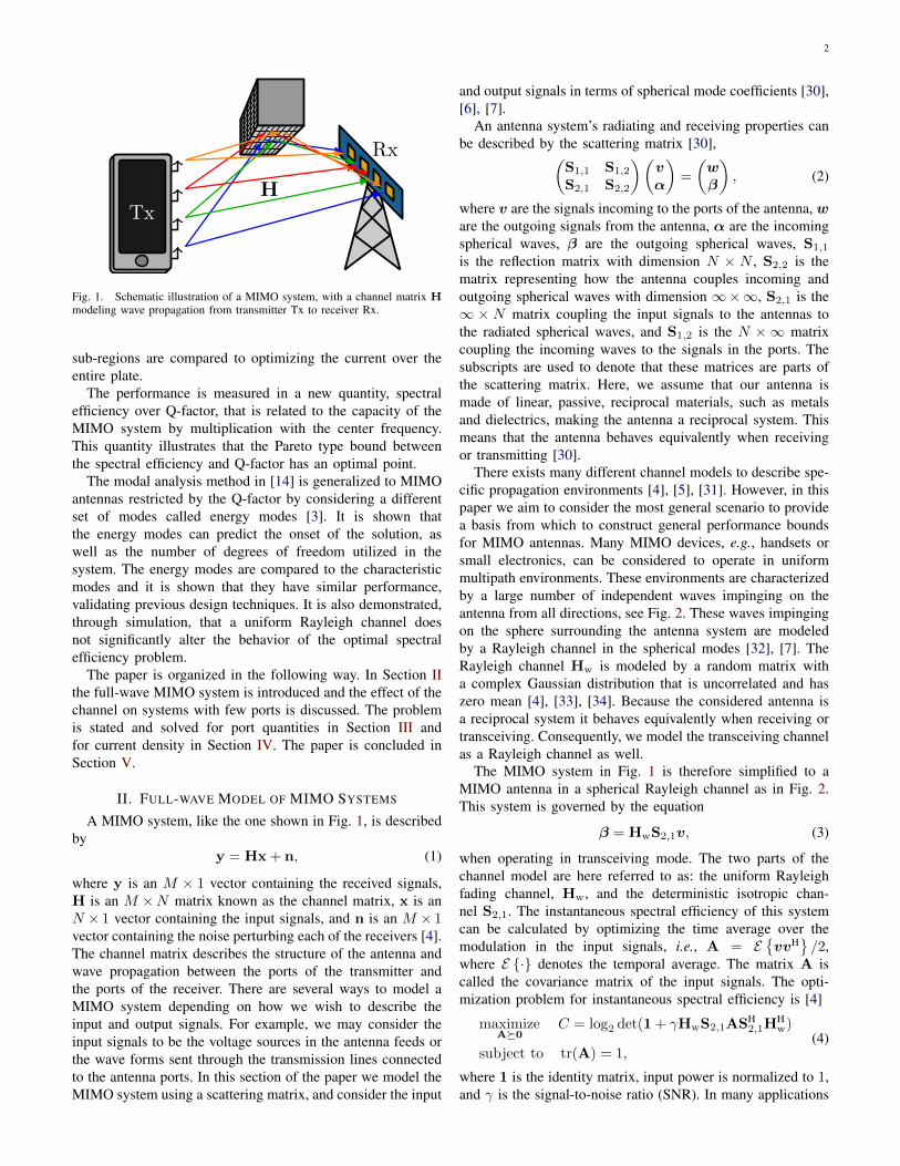
Fig. 1. Schematic illustration of a MIMO system, with a channel matrix Hmodeling wave propagation from transmitter Tx to receiver Rx.

sub-regions are compared to optimizing the current over theentire plate.

The performance is measured in a new quantity, spectralefficiency over Q-factor, that is related to the capacity of theMIMO system by multiplication with the center frequency.This quantity illustrates that the Pareto type bound betweenthe spectral efficiency and Q-factor has an optimal point.

The modal analysis method in [14] is generalized to MIMOantennas restricted by the Q-factor by considering a differentset of modes called energy modes [3]. It is shown thatthe energy modes can predict the onset of the solution, aswell as the number of degrees of freedom utilized in thesystem. The energy modes are compared to the characteristicmodes and it is shown that they have similar performance,validating previous design techniques. It is also demonstrated,through simulation, that a uniform Rayleigh channel doesnot significantly alter the behavior of the optimal spectralefficiency problem.

The paper is organized in the following way. In Section IIthe full-wave MIMO system is introduced and the effect of thechannel on systems with few ports is discussed. The problemis stated and solved for port quantities in Section III andfor current density in Section IV. The paper is concluded inSection V.

II. FULL-WAVE MODEL OF MIMO SYSTEMS

A MIMO system, like the one shown in Fig. 1, is describedby

y = Hx + n, (1)

where y is an M × 1 vector containing the received signals,H is an M ×N matrix known as the channel matrix, x is anN × 1 vector containing the input signals, and n is an M × 1vector containing the noise perturbing each of the receivers [4].The channel matrix describes the structure of the antenna andwave propagation between the ports of the transmitter andthe ports of the receiver. There are several ways to model aMIMO system depending on how we wish to describe theinput and output signals. For example, we may consider theinput signals to be the voltage sources in the antenna feeds orthe wave forms sent through the transmission lines connectedto the antenna ports. In this section of the paper we model theMIMO system using a scattering matrix, and consider the input

and output signals in terms of spherical mode coefficients [30],[6], [7].

An antenna system’s radiating and receiving properties canbe described by the scattering matrix [30],(

S1,1 S1,2

S2,1 S2,2

)(vα

)=

(wβ

), (2)

where v are the signals incoming to the ports of the antenna,ware the outgoing signals from the antenna, α are the incomingspherical waves, β are the outgoing spherical waves, S1,1

is the reflection matrix with dimension N × N , S2,2 is thematrix representing how the antenna couples incoming andoutgoing spherical waves with dimension ∞×∞, S2,1 is the∞× N matrix coupling the input signals to the antennas tothe radiated spherical waves, and S1,2 is the N ×∞ matrixcoupling the incoming waves to the signals in the ports. Thesubscripts are used to denote that these matrices are parts ofthe scattering matrix. Here, we assume that our antenna ismade of linear, passive, reciprocal materials, such as metalsand dielectrics, making the antenna a reciprocal system. Thismeans that the antenna behaves equivalently when receivingor transmitting [30].

There exists many different channel models to describe spe-cific propagation environments [4], [5], [31]. However, in thispaper we aim to consider the most general scenario to providea basis from which to construct general performance boundsfor MIMO antennas. Many MIMO devices, e.g., handsets orsmall electronics, can be considered to operate in uniformmultipath environments. These environments are characterizedby a large number of independent waves impinging on theantenna from all directions, see Fig. 2. These waves impingingon the sphere surrounding the antenna system are modeledby a Rayleigh channel in the spherical modes [32], [7]. TheRayleigh channel Hw is modeled by a random matrix witha complex Gaussian distribution that is uncorrelated and haszero mean [4], [33], [34]. Because the considered antenna isa reciprocal system it behaves equivalently when receiving ortransceiving. Consequently, we model the transceiving channelas a Rayleigh channel as well.

The MIMO system in Fig. 1 is therefore simplified to aMIMO antenna in a spherical Rayleigh channel as in Fig. 2.This system is governed by the equation

β = HwS2,1v, (3)

when operating in transceiving mode. The two parts of thechannel model are here referred to as: the uniform Rayleighfading channel, Hw, and the deterministic isotropic chan-nel S2,1. The instantaneous spectral efficiency of this systemcan be calculated by optimizing the time average over themodulation in the input signals, i.e., A = E

vvH

/2,

where E · denotes the temporal average. The matrix A iscalled the covariance matrix of the input signals. The opti-mization problem for instantaneous spectral efficiency is [4]

maximizeA0

C = log2 det(1 + γHwS2,1ASH2,1H

Hw)

subject to tr(A) = 1,(4)

where 1 is the identity matrix, input power is normalized to 1,and γ is the signal-to-noise ratio (SNR). In many applications

3

Rx

β

α

Tx

vw

Fig. 2. Schematic illustration of a MIMO antenna modeled using ascattering matrix (2). The incoming and outgoing signals are depicted forthe transceiving antenna as v and w, and for the spherical channel as αand β, respectively.

the channel Hw changes over time. It is then necessaryto consider the ergodic spectral efficiency, i.e., the spectralefficiency averaged over channel realizations, C = E C.

It was shown in [7] that the spectral efficiency for systemswith high SNR can be decomposed into a deterministic partdescribing the antenna and a random part independent ofthe antenna, see Appendix A. The physics of maximizingspectral efficiency are therefore independent of perturbinguniform channels, such as the Rayleigh channel. This isverified numerically in Section III-A. We will therefore usethe matrix S2,1 as the channel matrix for our calculations(Hw = 1).

Modelling a MIMO system using a scattering matrix isuseful when studying channel phenomena. However, in thispaper, we focus on how the design of a MIMO antenna impactsoptimal spectral efficiency. Consider the region in Fig. 3a, wewant to analyze how to construct the most effective MIMOantenna within this region. We must therefore switch ourmodelling from scattering parameters to quantities that let usincorporate antenna design as a variable.

The S1,1 part of the scattering matrix relation (2) can berewritten in terms of port quantities

zi = v, (5)

where v are the port voltages, i are the port currents, and zis the network impedance matrix [35], [36]. Here, we havemoved our perspective to Fig. 3b. In this case, the channelmatrix S2,1 is written as the connection between the portvoltages and the outgoing spherical waves. We will denotethis matrix s for simplicity, defined in Section III.

The network impedance matrix can either be calculatedfrom the (measured) scattering matrix or from a full-wave EMmodel. This is useful when studying a fixed set of antennas,as is done in Section III. We can further rewrite (5) in termsof meshed structures in order to use full-wave electromag-netic simulation techniques. In this paper we use method ofmoments (MoM) to simulate our systems, rewriting (5) as,

ZI = V, (6)

where I is the current column matrix, V is the excitationcolumn matrix, and Z is the impedance matrix [37], seeAppendix B. This equation models the case in Fig. 3c, where

antennadesignregion

(a)

V1+− V2

+−

(b)

J(r)

(c)

Fig. 3. Possible full-wave models of a transmitter Tx from Fig. 2. (a) Anantenna design region to be occupied by a MIMO system. (b) Two dipoles offixed geometry are considered within the design region. The feeding voltages,confined to the blue regions, are controllable variables to be optimized formaximum capacity. (c) The current density, confined to the green region, isthe controllable quantity. An optimized current is considered to be impressedin vacuum, the uncontrollable region is made from a given, yet arbitrary,material.

the current can exist everywhere inside the design region. Thecurrent can be split into regions that are controlled or passivelyexcited by the controlled region [29]. Similarly to the portcase, the channel matrix S2,1 is in this case written as theconnection between the currents on the antenna to the modesin the far field and will be called matrix S throughout thepaper. This formulation is very useful when optimizing thecurrent to study all possible antenna structures in a region,which is done in Section IV.

III. ARRAY ANTENNA EXCITATION

In this section we optimize the excitation of a fixed antennageometry, see Fig. 3b, when the antenna is placed in a deter-ministic isotropic channel. The maximum capacity given by aset of feeding ports is studied when the antenna’s bandwidthfor each port is prescribed and represented by the Q-factor.These fixed geometries are used to convey an intuition of howto induce optimal spectral efficiency.

The current density on an antenna structure is modeled asa linear combination of currents excited by localized feeders,so-called port modes [38], see Fig. 3b,

I = Z−1Cv =∑p

vpIp, (7)

where each port mode Ip corresponds to a unitary excitationof the p-th port, Z is the impedance matrix introduced in (6),and C ∈ 0, 1M×P is an indexation matrix defined element-wise as

Cmp =

1 p-th port is placed at m-th position,0 otherwise. (8)

A remarkable advantage of the port-mode representation isthe reduction of the original M ×M matrices, i.e., of numberof degrees of freedom, to P × P , the number of ports. Theconstruction of the impedance matrix (6) prior the reductioninto port modes (7) is needed since it represents the full-wave electromagnetic behavior of the systems. The values ofphysical quantities defined in MoM-like (6) and port-like (5)representations are equivalent. To illustrate the transformationlet M = MH ∈ CM×M represent a generic MoM operator,

4

such as the reactance matrix X. The following quadratic formsmap this operator to its port equivalent, m ∈ CP×P ,

m =1

2IHMI =

1

2vHmv, (9)

wherem = CHZ−HMZ−1C. (10)

Notice that the port-mode representation (10) changes thephysical units from Ohms for operator M to Siemens for portoperator m.

Spectral efficiency is calculated through the covariance ofthe input signals. The quadratic forms that typically calculateantenna quantities can be rewritten in terms of the covarianceof the port voltages. Conveniently, the port voltages is the onlypart of the antenna expressions that vary in time, therefore thetemporal average can be confined to this variable. For examplethe input power can be written as,

1

2EvHrv

=

1

2tr(EvHrv

)=

1

2tr(ErvvH) = tr(ra) = Pr,

(11)

where a = EvvH

/2 is the covariance of the port voltages,

Pr is the radiated power, and the cyclic properties of thetrace have been utilized. We assume the materials used in theantenna are lossless, therefore the radiated and input poweris the same. This enables the real part of the impedancematrix, z = r + jx, to be expanded in the spherical modesas r = sHs. The matrix s is the same matrix as the de-terministic isotropic channel matrix, which can be calculatedthrough (10), s = SZ−1C, see Appendix B for the definitionof matrix S [39], [6].

Applying the change of basis (9) and writing the problemin trace formulation, the spectral efficiency calculation (4) canbe written in the port-mode basis as

maximizea

log2 det(1 + γsasH)

subject to tr(ra) = 1.(12)

Here, the total radiated power is normalized to unity,Pr = 1 W. This problem is only restricted by the input powerto each port.

Antennas are most often optimized given certain restrictionsto their performance quantities, the formulation of (12) enablesus to add such restrictions as additional constraints. In thispaper we investigate how bandwidth restrictions affect spectralefficiency optimization.

The Q-factor is an antenna quantity that estimates thefractional bandwidth [1], [23], see its definition in Appendix C.The connection between the Q-factor and the bandwidth isexplicit for single input systems in free space but there existsno explicit quantity or expression for calculating the bandwidthfor MIMO systems. However, each of the ports of a MIMOsystem is a single input system, if taken in isolation. Therefore,each of these ports have a well defined Q-factor based on theirinputs. We can require a certain Q-factor of each of the portsin the system as a way of implicitly placing a requirement onthe total systems bandwidth. However, the Q-factor is usuallydefined in relation to the system at resonance. For a multi-port

system a single resonance of the total current is not alwaysdesired, thus the Q-factor of the system must be estimated ina different way. Here, we use the average of the magnetic andelectric stored energies over the radiated power to estimate thebandwidth. This corresponds to adding the condition,

EvHwxv

2Pr

=tr(wxa)

Pr≤ Q, (13)

where wx is the matrix giving the reactive power of theaveraged stored energy, see Appendix C, and Q is the requiredQ-factor.

The Q-factor constraint (13) is added to (12) to create theoptimization problem that is investigated in this paper,

maximizea

log2 det(1 + γsasH)

subject to tr(ra) = 1,

tr(wxa) ≤ Q,a 0.

(14)

A problem of this form can be solved using commerciallyavailable software, such as MATLAB software for disciplinedconvex programming (CVX) [40], see [13]. However, it can besolved much more efficiently, and in such a way as to providegreater physical insight, using the method presented in [14].The method is based on constructing a convex dual problemthat can be solved semi-analytically. A brief outline of thatprocedure is covered here.

Dual problems are constructed from an original optimiza-tion problem by forming linear combinations between theconstraints of the original problem. The solution to the dualproblem will therefore always have a value that bounds thesolution of the original problem (14). However, there may exista duality gap between the two solutions leading to a “loose”bound on the optimization problem [25]. The results presentedin this paper have been verified numerically in CVX and noduality gap was observed.

To formulate the dual of the optimization problem (14) wetake an affine combination of the conditions restricting theoriginal problem,

minν

maxa

log2 det(1 + γsasH)

subject to tr[(νr +Q−1wx

)a]

= (ν + 1),

a 0.

(15)

This problem is convex in the variable ν. The tightest boundon the solution of the original problem is found when thedual problem is minimized over ν [25]. The solution to thisproblem is found in [14] by incorporating the matrices of thefirst condition in (15) into the channel matrix of the system,see Appendix D. This recasts the system in a form where itcan be solved by water-filling [4], [5].

The water-filling procedure is carried out by taking thesingular value decomposition of the channel matrix. Each sin-gular value represents the loss associated with feeding powerin its corresponding mode. The optimal solution is found byiteratively allocating energy to the channels associated withthe largest singular values [4], [5], [14]. The algorithm can be

5

10−2 10−1 100 101 102 103 10410−3

10−2

10−1

100

101

102

103

ν

σ2 n

w1 = 0.01Q

w2 = 0.1Q

w3 = Q

w4 = 10Q

w5 = 100Q1 2 3 4 50

20

40

60γ = 200ν = 1.9

1 2 3 4 505

101520

γ = 20ν = 4.5

1 2 3 4 50

2

4

6γ = 2ν = 22.1

Fig. 4. The singular values (17) as a function of ν for different energymode values. The three insets show water-filling solutions (15) at optimalν ∈ 22.1, 4.5, 1.9 for three different SNR values, γ ∈ 2, 20, 200. Forγ ∈ 2, 20 the weakest mode, w5, is not used because the SNR value isinsufficient.

expressed as,

maximize

N∑n=1

log2

(1 + anγσ

2n

)subject to

N∑n=1

an = 1,

(16)

where an ≥ 0 is the power allocation fraction in each channel,and σn is the singular value of the corresponding channel.

The singular values of the channel matrix are

σ2n =

1 + ν

wn/Q+ ν, (17)

where wn are the eigenvalues of a set of modes, here referredto as energy modes [3]. The energy modes are calculatedthrough the generalized eigenvalue problem, defined here overport mode matrices,

wxvn = wnrvn, (18)

where vn are the modal port voltages. These modes are similarto characteristic modes [41] in the sense that they have theproperty of orthogonal radiation patterns. In addition, theyminimize the total energy stored by the antenna. This has theeffect of implicitly maximizing the bandwidth of the modeswith the lowest eigenvalues.

The singular values σ2n from (17) are depicted in Fig. 4

as a function of ν for energy modes with eigenvalues chosenas wn/Q = 10n−3, where n ∈ 1, . . . , 5. The water-fillingsolutions (16) of (15) at the optimal ν are shown in insetsfor the SNR values γ ∈ 2, 20, 200. We observe that theoptimal ν decreases with increasing γ and that strong channels,corresponding to wn/Q ≤ 1, are included for all considered γ,whereas the weaker channels, wn/Q > 1, are only includedfor high γ. The singular values approach unity as ν → ∞with the explicit equal power allocation solution for N equalchannels

C = N log2

(1 +

γ

N

). (19)

0.2 0.4 0.6 0.8 1 1.2 1.4 1.6 1.8 2100

101

102

2.8

31

3.2

9.6

5.1

w1 w2

d/L

wn

V1 V2 L V1 V2

d

L

Fig. 5. The eigenvalues of the energy port-modes wn evaluated by (18)for an array of two dipoles placed in-parallel, separated by the dis-tance d (see the insets). The values of wn are marked for separationdistances d/L ∈ 0.3, 0.6, 0.9.

This is also the explicit solution for the case withmax(wn/Q) ≤ 1, because the Q-factor constraint in (14) istrivially satisfied. This suggests that the number of availablechannels for a given Q-factor can be estimated by studyingthe energy mode eigenvalues. Modes with wn/Q ≤ 1 can beconsidered available and will always be used by the systemto induce maximum spectral efficiency. The energy modesnot only simplify the optimization problem for maximumcapacity to water-filling solutions (16) but also provide aphysical interpretation of the results. Let us now consider a fewexamples to see how the solution to this optimization problembehaves.

A. Example – Two Dipoles of Variable Separation Distance

The first example deals with two thin-strip dipoles of(resonant) length L/λ = 0.49 and width L/W = 50. Thedipoles are made of perfect electric conductor (PEC) andseparated by the distance d swept in the interval d/L ∈ [0, 2].

The sole input into the optimization procedure is the setof energy mode eigenvalues (18). Their dependence on theseparation distance d/L is shown in Fig. 5. There are twotypes of modes, in-phase and out-of-phase modes, whichbecome degenerated at d/L ≈ 0.9 and d/L ≈ 1.9. Thesmallest eigenvalue of the in-phase mode is w1 ≈ 3 for smalldistances whereas the out-of-phase mode w2 increases rapidlyas d/L → 0. This implies an onset around Q ≈ 3 with aspectral efficiency of a single channel, N = 1, used in (19).The out-of-phase mode starts to contribute for larger Q-factorsas wn/Q decreases in the channel singular values (17), seealso Fig. 4 and the insets in Fig. 6 with the water-fillingsolutions for Q = 3 and Q = 10. At the degeneracy aroundd/L ≈ 0.9 the modes contribute equally following the spectralefficiency (19) from two equal channels (N = 2) as Qincreases. For larger distances, the two modes have similareigenvalues wn as the mutual coupling diminishes.

The maximum spectral efficiency calculated with (14) isdepicted in Fig. 6 for γ = 20 and spacing d/L = 0.3 as afunction of the Q-factor. The onset is bounded by the lower

6

3 4 5 6 7 8 9 10 11 123

4

5

6

7

N = 1

N = 2

CHw

C1

CHw± std.

Q

C(bits/s/Hz)

V1 V2

d

L

1 20

10

20 Q = 3

1 20

10

20 Q = 10

Fig. 6. The maximal ergodic spectral efficiency of two centrally fed dipoles inRayleigh fading (the blue dashed line) and deterministic isotropic (the solidred line) channels. The gray area denotes the one standard deviation limitof the channel realizations. The dipoles have electrical size L/λ = 0.49,are separated d/L = 0.3, and the SNR has been set to γ = 20. Thedashed horizontal lines correspond to one and two ideal equal power allocationchannels (19). The two insets show the water-filling solutions for Q = 3 andQ = 10.

bound on the Q-factor, determined from the smallest eigen-value wn. For two dipoles separated by distance d/L ≈ 0.3that bound is just below Q = 3 as seen in Fig. 5. Thissupports previous observations [42], [43] that two mutuallycoupled dipoles might have lower Q than a single dipole (hereQ ≈ 5). After the onset the spectral efficiency C increasestowards C = 6.9 which is reached for Q ≈ 31. The horizontaldashed lines in Fig. 6 show the spectral efficiency of one andtwo ideal equal power allocation channels that do not takeinto account antenna geometry or channel effects. These linesserve as an indicator of how many pathways the system isutilizing [14]. The Q-factor values at which the two dipolesproduce the optimal spectral efficiency of either one or twoideal channels correspond perfectly to the first and secondeigenvalue from Fig. 5. The two dipoles can be seen to havesolutions in between one and two ideal channels. Indicatingthat they are utilizing two channel pathways.

The optimization problem (15) can be solved for a MIMOantenna in a complex propagation channel, by multiplying thematrix s with the channel matrix. However, the singular valuedecomposition (SVD) of the channel matrix (17) can no longerbe found efficiently. For each ν considered in the optimizationprocess, the SVD must be calculated numerically. In Fig. 6,the maximum spectral efficiency in a uniform Rayleigh fadingchannel and a deterministic isotropic channel are comparedfor the two dipoles. It can be seen that the antenna in thedeterministic channel follows the behaviour of the system ina Rayleigh channel. This shows that the deterministic channelcan be used to estimate the maximum spectral efficiencycharacteristics of an electrically small antenna design problemin a uniform Rayleigh fading multipath environment.

In Fig. 6, the spectral efficiency grows with Q. This canbe misleading, and does not mean that higher capacity canbe achieved by a narrow-band system. Spectral efficiency isa measure of the maximum bit rate that can be achieved

2.5 3 3.5 4 4.5 5 5.5 6 6.50.7

0.9

1.1

1.3

1.5

1.7

1.9

N = 1

N=2

d/L = 0.1 · · · d/L = 0.3 · · · d/L = 1.0

4.4

4.4

4.4 4.5 5.1 5.66.2

6.7

6.96.7

d/L

=0.1

d/L

=0.5

d/L

=0.6

d/L

=0.7

d/L

=0.8

d/L

=0.9

d/L

=1.0

Q

C/Q

Fig. 7. The maximal spectral efficiency over Q for two thin-strip dipolesof separation distance d. Dot marks with numbers correspond to particularspectral efficiencies, evaluated at C/Q maximum. The SNR has been set toγ = 20.

on a 1 Hz bandwidth. By allowing a higher Q-factor in theoptimization problem the solution can concentrate all spectralefficiency to a specific frequency. The true capacity can becalculated from the spectral efficiency by multiplying it bythe bandwidth. An indication of the capacity can be found byconsidering the spectral efficiency divided by the required Q-factor, C/Q. This measure is adopted for the remaining resultsin the paper.

The spectral efficiency C over Q, evaluated via (14), fortwo dipoles as a function of their separation distance d/L isshown in Fig. 7. It is seen that there exists an optimal distance,d/L ≈ 0.3, for which C/Q is maximal. This is the distancewith the lowest possible eigenvalue in Fig. 5. All the curvesare bounded from the left by the fundamental bound on Q fortwo dipoles given by the lowest eigenvalue wn. The maximumspectral efficiency is bounded by (19) with N = 2, shown bya dashed curve, and is first reached for the degenerate casearound the distance d/L ≈ 0.9 with w1 = w2 ≈ 5.1, seeFig. 5. However, this curve does not dominate the others, eventhough it has the highest spectral efficiency. This is due tohigher Q of the dipoles. For distances between d/L = 0.3and d/L = 0.9, we see a gradual increase from the lowestQ = w1 with a N = 1 spectral efficiency (19) increasing totwo channels N = 2 as Q approaches w2.

When the dipoles are separated by a large distance they actas separate radiators and do not improve their joint Q-factor.This indicates that there is a trade-off between decoupling thedipole radiators to improve spectral efficiency and utilizingtheir mutual coupling to improve their bandwidth [2].

B. Example – Two Dipoles Rotated by An Arbitrary Angle

Here, we study the dependence on the angle betweenthe dipoles. The separation distance between two dipoles isfixed to the optimal value from the previous example, i.e.,d/L = 0.3. The dipoles are of the same dimensions, locatedat x = −d/2 and x = d/2, and the left dipole is parallel tothe z-axis. The axis of rotation for the right dipole coincideswith the x-axis, see the insets of Fig. 9.

7

0 π/8 π/4 3π/8 π/22

5

10

20

w1 w2

ϕ

wn

V1 V2 L

d

ϕ = 0 V1 V2

ϕ = π/2

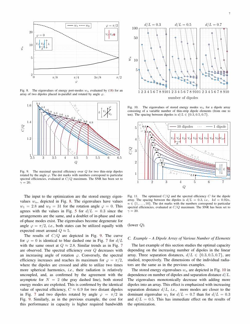
Fig. 8. The eigenvalues of energy port-modes wn evaluated by (18) for anarray of two dipoles placed in-parallel and rotated by angle ϕ.

2.5 3 3.5 4 4.5 5 5.5 6 6.51

1.2

1.4

1.6 ϕ = 0 · · · ϕ = π/24.4

4.44.6

4.95.3 5.6

5.96.2

6.66.8 6.9

N=1

N=2

Q

C/Q

ϕ

V1V2

L

Fig. 9. The maximal spectral efficiency over Q for two thin-strip dipolesrotated by the angle ϕ. The dot marks with numbers correspond to particularspectral efficiencies, evaluated at C/Q maximum. The SNR has been set toγ = 20.

The input to the optimization are the stored energy eigen-values wn, depicted in Fig. 8. The eigenvalues have valuesw1 = 2.8 and w2 = 31 for the rotation angle ϕ = 0. Thisagrees with the values in Fig. 5 for d/L = 0.3 since thearrangements are the same, and a doublet of in-phase and out-of-phase modes exist. The eigenvalues become degenerate forangle ϕ = π/2, i.e., both states can be utilized equally withexpected onset around Q ≈ 5.

The results of C/Q are depicted in Fig. 9. The curvefor ϕ = 0 is identical to blue dashed one in Fig. 7 for d/Lwith the same onset at Q ≈ 2.8. Similar trends as in Fig. 7are observed. The spectral efficiency over Q decreases withan increasing angle of rotation ϕ. Conversely, the spectralefficiency increases and reaches its maximum for ϕ = π/2,where the dipoles are crossed and able to utilize two timesmore spherical harmonics, i.e., their radiation is relativelyuncoupled, and, as confirmed by the agreement with theasymptote for N = 2 (the gray dashed line), both storedenergy modes are exploited. This is confirmed by the identicalvalue of spectral efficiency, C ≈ 6.9 for two distant dipolesin Fig. 7 and two dipoles rotated by angle ϕ = π/2 inFig. 9. Similarly, as in the previous example, the cost forthis performance in capacity is higher required bandwidth

1 2 3 4 5 6 7 8 910

5

10

50

100

wn

d/L = 0.3

1 2 3 4 5 6 7 8 910

number of dipoles

d/L = 0.5

1 2 3 4 5 6 7 8 910

d/L = 0.7

Fig. 10. The eigenvalues of stored energy modes wn for a dipole arrayconsisting of a variable number of thin-strip dipole elements (from one toten). The spacing between dipoles is d/L ∈ 0.3, 0.5, 0.7.

1 2 3 4 5 6 7

1

2

3

4

5

N = 1

N=

2

N = 5

N = 10

10 dipoles · · · 1 dipole

4.4

4.4

5.2

6.1

6.6

6.9

7.6

8.28.6

8.6

Q

C/Q

V1 L

V1 V2 V3 V4 V5 V6 V7 V8 V9 V10

d

Fig. 11. The optimized C/Q and the spectral efficiency C for the dipolearray. The spacing between the dipoles is d/L = 0.3, i.e., kd = 0.92n,n ∈ 1, . . . , 10. The dot marks with the numbers correspond to particularspectral efficiencies, evaluated at C/Q maximum. The SNR has been set toγ = 20.

(lower Q).

C. Example – A Dipole Array of Various Number of Elements

The last example of this section studies the optimal capacitydepending on the increasing number of dipoles in the lineararray. Three separation distances, d/L ∈ 0.3, 0.5, 0.7, arestudied, respectively. The dimensions of the individual radia-tors are the same as in the previous examples.

The stored energy eigenvalues wn are depicted in Fig. 10 independence on number of dipoles and separation distance d/L.The eigenvalues monotonically decrease with adding moredipoles into an array. This effect is emphasized with increasingseparation distance d/L, i.e., more modes are closer to thedominant eigenvalue w1 for d/L = 0.7 than for d/L = 0.3and d/L = 0.5. This has immediate effect on the results ofthe optimization.

8

1 2 3 4 5 6 7

1

2

3

4

5

6

N = 1

N=

2

N=5

N = 10

10 dipoles · · · 1 dipole

4.39

5.11

6.52

7.13

8.21

8.57

9.45

9.79

10.1

10.6

Q

C/Q

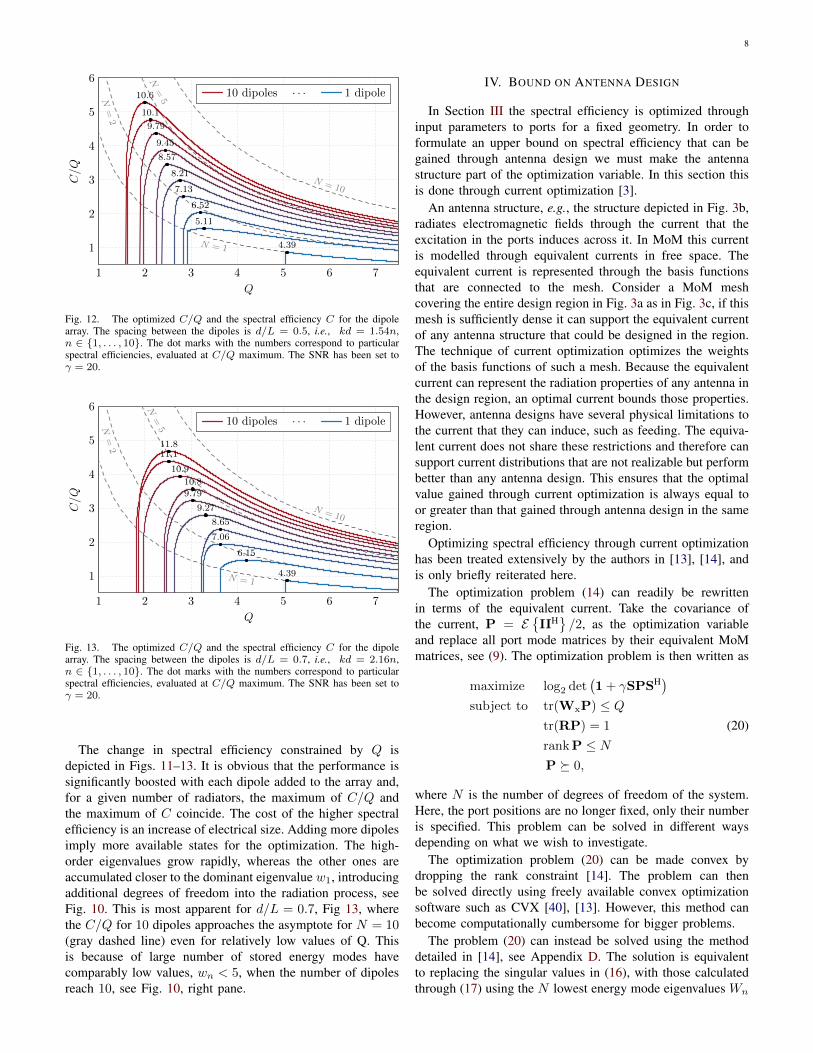
Fig. 12. The optimized C/Q and the spectral efficiency C for the dipolearray. The spacing between the dipoles is d/L = 0.5, i.e., kd = 1.54n,n ∈ 1, . . . , 10. The dot marks with the numbers correspond to particularspectral efficiencies, evaluated at C/Q maximum. The SNR has been set toγ = 20.

1 2 3 4 5 6 7

1

2

3

4

5

6

N = 1

N=

2

N=5

N = 10

10 dipoles · · · 1 dipole

4.39

6.15

7.06

8.65

9.27

9.7910.8

10.9

11.111.8

Q

C/Q

Fig. 13. The optimized C/Q and the spectral efficiency C for the dipolearray. The spacing between the dipoles is d/L = 0.7, i.e., kd = 2.16n,n ∈ 1, . . . , 10. The dot marks with the numbers correspond to particularspectral efficiencies, evaluated at C/Q maximum. The SNR has been set toγ = 20.

The change in spectral efficiency constrained by Q isdepicted in Figs. 11–13. It is obvious that the performance issignificantly boosted with each dipole added to the array and,for a given number of radiators, the maximum of C/Q andthe maximum of C coincide. The cost of the higher spectralefficiency is an increase of electrical size. Adding more dipolesimply more available states for the optimization. The high-order eigenvalues grow rapidly, whereas the other ones areaccumulated closer to the dominant eigenvalue w1, introducingadditional degrees of freedom into the radiation process, seeFig. 10. This is most apparent for d/L = 0.7, Fig 13, wherethe C/Q for 10 dipoles approaches the asymptote for N = 10(gray dashed line) even for relatively low values of Q. Thisis because of large number of stored energy modes havecomparably low values, wn < 5, when the number of dipolesreach 10, see Fig. 10, right pane.

IV. BOUND ON ANTENNA DESIGN

In Section III the spectral efficiency is optimized throughinput parameters to ports for a fixed geometry. In order toformulate an upper bound on spectral efficiency that can begained through antenna design we must make the antennastructure part of the optimization variable. In this section thisis done through current optimization [3].

An antenna structure, e.g., the structure depicted in Fig. 3b,radiates electromagnetic fields through the current that theexcitation in the ports induces across it. In MoM this currentis modelled through equivalent currents in free space. Theequivalent current is represented through the basis functionsthat are connected to the mesh. Consider a MoM meshcovering the entire design region in Fig. 3a as in Fig. 3c, if thismesh is sufficiently dense it can support the equivalent currentof any antenna structure that could be designed in the region.The technique of current optimization optimizes the weightsof the basis functions of such a mesh. Because the equivalentcurrent can represent the radiation properties of any antenna inthe design region, an optimal current bounds those properties.However, antenna designs have several physical limitations tothe current that they can induce, such as feeding. The equiva-lent current does not share these restrictions and therefore cansupport current distributions that are not realizable but performbetter than any antenna design. This ensures that the optimalvalue gained through current optimization is always equal toor greater than that gained through antenna design in the sameregion.

Optimizing spectral efficiency through current optimizationhas been treated extensively by the authors in [13], [14], andis only briefly reiterated here.

The optimization problem (14) can readily be rewrittenin terms of the equivalent current. Take the covariance ofthe current, P = E

IIH/2, as the optimization variable

and replace all port mode matrices by their equivalent MoMmatrices, see (9). The optimization problem is then written as

maximize log2 det(1 + γSPSH)

subject to tr(WxP) ≤ Qtr(RP) = 1

rankP ≤ NP 0,

(20)

where N is the number of degrees of freedom of the system.Here, the port positions are no longer fixed, only their numberis specified. This problem can be solved in different waysdepending on what we wish to investigate.

The optimization problem (20) can be made convex bydropping the rank constraint [14]. The problem can thenbe solved directly using freely available convex optimizationsoftware such as CVX [40], [13]. However, this method canbecome computationally cumbersome for bigger problems.

The problem (20) can instead be solved using the methoddetailed in [14], see Appendix D. The solution is equivalentto replacing the singular values in (16), with those calculatedthrough (17) using the N lowest energy mode eigenvalues Wn

9

0.2 0.4 0.6 0.8 1 1.2 1.4 1.6 1.8 2100

101

102

103

W1 = 3.9

W2 = 9.1

W3 = 15

ka

Wn

I1 I2 I3

Fig. 14. Energy mode eigenvalues Wn (21) for a rectangular region withside lengths ` × `/2, the first three eigencurrents at ka = 1 are shown aswell.

calculated by the generalized eigenvalue problem,

WxIn = WnRIn. (21)

These modes have the same properties as their port equiva-lents (18), i.e., orthogonal radiation patterns and minimizationof the total stored energy.

A. Modal Analysis for a rectangular plate

Fig. 14 depicts the eigenvalues of energy modes for arectangular plate with side lengths ` × `/2 as a functionof electrical size 0.2 ≤ ka ≤ 2. The modal behaviour oftwo electric dipoles and one magnetic dipole dominate forelectrically small structures, where the scaling Wn ∼ (ka)−3

is found [44], [45]. Higher-order modes have very largeeigenvalues Wn and require similarly high Q to contribute.The energy-mode eigenvalues Wn decrease with increasingelectrical size and several modes are available for larger ka.For ka = 1, we have the first eigenvalue W1 ≈ 4, proposingan onset around Q = 4, and two additional eigenvalues at 9and 15 indicate three independent channels below Q = 15,see Fig. 15.

When optimizing over the current density the number ofchannels in (4) can no longer be considered small. Therefore,we must analyze the impact of the Rayleigh channel on theoptimization results. Consider (20) with the objective function,

CHw= log2 det

(1 + γHwSPSHHH

w

). (22)

4 5 6 7 8 9 10

4

6

8

10

N = 1

N = 2

N = 3

CHw

C1

CHw± std.

Q

C(bits/s/Hz)

Ω

`/2

`

Fig. 15. Maximum ergodic spectral efficiency of a ka = 1, ` × `/2 platein a uniform Rayleigh fading channel (blue dashed line) and a deterministicisotropic channel (solid red line). The gray area denotes one standard deviationfrom the average of the Rayleigh channel case. The dashed horizontal linescorrespond to one, two, and three ideal equal power allocation channels [14].

This can be done by numerically calculating the SVD of thechannel matrix for each ν.

In Fig. 15 the current on a ka = 1 plate has been optimizedfor maximal spectral efficiency with and without the inclusionof a uniform Rayleigh channel. The average of the uniformRayleigh fading channel realizations has the same performanceas the plate in the deterministic isotropic spherical channel.This supports the claims in [13], [14] that the Rayleigh channelcan be neglected when studying the fundamentals of antennadesign for optimal spectral efficiency in uniform multipathenvironments.

The standard deviation of the Rayleigh channel realizationsfor the plate in Fig. 15 is significantly smaller than what can beseen for two dipoles in Fig. 6. This is due to the added degreesof freedom in optimizing an entire plate. The plate can supporthigher order modes at lower Q-values and its current can betailored to specific channel realizations.

B. Sub-region Energy modes

Antennas inside communication devices are, in general,much smaller than the total device size [46]. This meansthat only a sub-region of the device is dedicated to antennadesign. The antennas therein excite currents across the entiredevice that contribute to communication. From an optimizationperspective this can be seen as only controlling the currentwithin the antenna sub-region. The optimization of arraysthrough their port quantities in Section III is similar to thisconcept. The ports control the current on the dipole on a verysmall sub-region of the antenna. In this section this concept isgeneralized to controlling the current in larger sub-regions, seeFig. 3c. Optimizing the current on a sub-region for maximalspectral efficiency calculates a bound on the spectral efficiencyavailable from designing an antenna in a sub-region of adevice. This is interesting to investigate since bandwidth andQ-factor are usually harshly restricted by reducing the antennasize [20], [47].

Consider the placement of sub-regions for antenna design

10

1 2 3 4 5 6 7

100

101

102

103

n

Wn

Sphere

Plate

A

B

C

D

E

1A 1B 1C 1D E

`

`/2

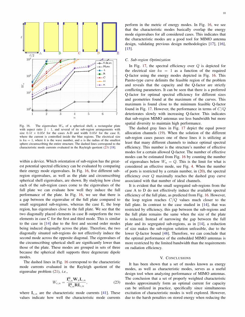
Fig. 16. The eigenvalues Wn of a spherical shell, a rectangular platewith aspect ratio 2 : 1, and several of its sub-region arrangements withsize 0.1` × 0.05` for the cases A-D and width 0.05` for the case E,where the current is controlled inside the blue regions. The electrical sizeis ka = 1, where k is the wave number, and a is the radius of the smallestsphere circumscribing the entire structure. The dashed lines correspond to thecharacteristic mode currents evaluated in the Rayleigh quotient (23) [18].

within a device. Which orientation of sub-region has the great-est potential spectral efficiency can be evaluated by comparingtheir energy mode eigenvalues. In Fig. 16, five different sub-region eigenvalues, as well as the plate and circumscribingspherical shell eigenvalues, are shown. By studying how closeeach of the sub-region cases come to the eigenvalues of thefull plate we can evaluate how well they induce the fullperformance of the plate. In Fig. 16, we see that there isa gap between the eigenvalue of the full plate compared tosmall segregated sub-regions, whereas the case E, the loopregion, has eigenvalues close to the full plate. We see that thetwo diagonally placed elements in case B outperform the twoelements in case C for the first and third mode. This is similarto the case in [14] due to the first and second order modesbeing induced diagonally across the plate. Therefore, the twodiagonally situated sub-regions do not effectively induce thesecond mode across the opposite diagonal. The eigenvalues ofthe circumscribing spherical shell are significantly lower thanthose of the plate. These modes are grouped in sets of threebecause the spherical shell supports three degenerate dipolemodes.

The dashed lines in Fig. 16 correspond to the characteristicmode currents evaluated in the Rayleigh quotient of theeigenvalue problem (21), i.e.,

Wc,n =IHc,nWxIc,n

IHc,nRIc,n

, (23)

where Ic,n are the characteristic mode currents [41]. Thesevalues indicate how well the characteristic mode currents

perform in the metric of energy modes. In Fig. 16, we seethat the characteristic modes basically overlap the energymode eigenvalues for all considered cases. This indicates thatthe characteristic modes are a good tool for MIMO antennadesign, validating previous design methodologies [17], [16],[15].

C. Sub-region Optimization

In Fig. 17, the spectral efficiency over Q is depicted forthe electrical size ka = 1 as a function of the requiredQ-factor using the energy modes depicted in Fig. 16. ThisPareto-type curve delimits the feasible region of the problemand reveals that the capacity and the Q-factor are strictlyconflicting parameters. It can be seen that there is a preferredQ-factor for optimal spectral efficiency for different sizesand geometries found at the maximum of the curves. Thismaximum is found close to the minimum feasible Q-factorfound in Fig. 17. However, the performance in terms of C/Qdeteriorates slowly with increasing Q-factor. This indicatesthat sub-region MIMO antennas use less bandwidth but morespatial diversity to maintain high performance.

The dashed gray lines in Fig. 17 depict the equal powerallocation channels (19). When the solution of the differentsub-region cases passes one of these lines it is utilizing atleast that many different channels to induce optimal spectralefficiency. This number is the structure’s number of effectivemodes for a certain allowed Q-factor. The number of effectivemodes can be estimated from Fig. 16 by counting the numberof eigenvalues below Wn = Q. This is the limit for what isconsidered an effective mode, see Fig. 4. When the numberof ports is restricted by a certain number, in (20), the spectralefficiency over Q maximally reaches the dashed gray curveassociated with that number of ideal channels.

It is evident that the small segregated sub-regions from thecase A to D do not effectively induce the available spectralefficiency of the full plate, as predicted from Fig. 16. However,the loop region reaches C/Q values much closer to thefull plate. In contrast to the case studied in [14], that wasrestricted by efficiency, this gap between the sub-regions andthe full plate remains the same when the size of the plateis reduced. Instead of narrowing the gap between the fullplate and its segregated sub-regions, as in [14], a reductionof size makes the sub-region solution unfeasible, due to thelower Q-factor bound [48]. Therefore, we can conclude thatthe optimal performance of the embedded MIMO antennas ismore restricted by the limited bandwidth than the requirementson radiation efficiency.

V. CONCLUSIONS

It has been shown that a set of modes known as energymodes, as well as characteristic modes, serves as a usefuldesign tool when analyzing performance of MIMO antennas.The conclusion that a set of properly weighted characteristicmodes approximately form an optimal current for capacitycan be utilized in practice, specifically since simultaneousexcitation of characteristic modes is well explored. However,due to the harsh penalties on stored energy when reducing the

11

0 5 10 15 20 25 30 35 40 45 50

0.1

1

10

N=1

N = 5

N = 20

Q

C/Q

Sphere

Plate

A

B

C

D

E

a

Fig. 17. The optimal spectral efficiency over Q for the ka = 1 sphericalshell, plate with aspect ratio 2 : 1, and its sub-regions presented in Fig. 16, fordifferent Q-factor restrictions. The dashed gray lines correspond to increasingnumbers of ideal equal power allocation channels. The SNR has been set toγ = 20.

design region, it has been concluded that it is not possible toreach the full potential of the plate while only feeding it witha set of small segregated sub-regions. However, the use of aconnected loop region was shown to be much more efficient.

Spectral efficiency bounds of MIMO antennas in uniformRayleigh fading channels and a deterministic isotropic channelhave been considered when restricted by the Q-factor. It wasshown that the uniform Rayleigh fading channel does notaffect the characteristics of the spectral efficiency bound. ThePareto-type bound has been illustrated in spectral efficiencyover Q, where a certain Q-factor was shown to be Paretooptimal.

The modal analysis illustrated in this paper could also becarried out on designed antennas to evaluate their adherenceto the principals suggested here. Generalizing this methodto include several different design parameters remains aninteresting future prospect.

APPENDIX ARAYLEIGH CHANNEL CONTRIBUTION

To study the dependence of the system on the uniformRayleigh fading channel, consider a MIMO system with afinite and small number of ports N . Since the number ofports is small, the SNR can be considered to be large ineach port, i.e., γHwS2,1ASH

2,1HHw α1, α 1. The ergodic

spectral efficiency is then gained by averaging (4) over channelrealizations,

C = E

log2 det(γHwS2,1ASH2,1H

Hw)

= log2 det(γ) + E log2 det(Hw)+ E

log2 det(HH

w)

+ log2 det(S2,1ASH2,1).

(24)

The effect of the channel in such a system is only anadditive term in the spectral efficiency evaluation. Considerthe correlation loss, defined as

∆C = C − C1, (25)

where C1 is the equal power allocation solution. This quantityis independent of the additive channel contribution in (24).

This implies that the physics of maximizing ergodic spectralefficiency is independent of the channel in uniform multipathenvironment, as long as the number of ports in the system islow [7]. Note that (25) only contains a temporal average overthe input signals, significantly simplifying its evaluation.

APPENDIX BELECTRIC FIELD INTEGRAL EQUATION

All antenna structures in this paper are modeled as perfectlyconducting bodies with the electric field integral equation(EFIE), [37], which relates tangential component of incidentand scattered electric fields as

n×Ei (r) = −n×Es (r) , (26)

where Ei is the incident field, Es is the scattered field

Es (r) = −jkZ0

∫Ω

G (r, r′) · J (r′) dS′, (27)

Z0 is the impedance of vacuum, k is wavenumber, and Gdenotes the free-space dyadic Green’s function defined as

G (r, r′) =

(1 +∇∇k2

)e−jk|r−r

′|

4π |r− r′| (28)

with 1 being the identity dyadic.By applying a suitable set of basis functions

J(r) ≈N∑n=1

Inψn(r) (29)

and the same set as testing functions (Galerkin method), therelation (26) transforms into algebraic form

ZI = V, (30)

where the impedance matrix Z = [Znm] ∈ CN×N andexcitation vector V = [Vn] ∈ CN×1 are defined element-wiseas

Znm = −jkZ0

∫Ω

∫Ω

ψn (r)·G (r, r′)·ψm (r′) dS dS′, (31)

and

Vn =

∫Ω

ψn (r) ·Ei (r) dS, (32)

respectively.The real part R of the impedance matrix Z = R + jX can

be factorized asR = STS, (33)

where the matrix S is defined element-wise as

Sαn = k√Z0

∫Ω

ψn · u(1)α (kr) dS (34)

with u(1)α being the regular spherical waves, see [49] for

details.

12

APPENDIX CDEFINITION OF Q-FACTOR

The radiation Q-factor is defined as

Qrad =2ωmax Wm,We

Pr, (35)

where the stored magnetic and electric energies are

ωWm =1

8IH(ω∂X

∂ω+ X

)I, (36a)

ωWe =1

8IH(ω∂X

∂ω−X

)I, (36b)

the radiated power is defined as

Pr =1

2IHRI, (37)

and Z = R+jX is the impedance matrix, see Appendix B. Forpurposes of this paper, the stored energy matrix is introducedas

Wx =1

2ω∂X

∂ω, (38)

and the radiation Q-factor is rewritten as

Qrad = Q+Qt =ω (Wm +We)

Pr+ω|Wm −We|

Pr, (39)

where the first part (Q) belongs to the antenna itself andthe second part (Qt) belongs to a lumped element tuningan antenna to the resonance [1]. Generally, it holds thatQrad ≥ Q, and Qrad = Q only at the self-resonance of anantenna. In this paper, we use only the first part of (39), Q,since it is a low-bound estimate of an achievable Q-factorirrespective of how a multi-port antenna is tuned.

APPENDIX DSVD OF CHANNEL MATRIX

The optimal solution of (15) is found by writing the systemon the form (16). This is achieved through a change ofvariables. Define the matrix

rν =1

(ν + 1)

(νr +Q−1wx

). (40)

This matrix is positive semi-definite for sufficiently large an-tenna sizes, and appropriate values of ν. Positive semi-definitematrices can be decomposed with the Cholesky decomposi-tion, rν = bHb. With this decomposition the condition in (16)can be rewritten as,

EvHrνv

= tr(rνa) = tr(babH) = tr(a), (41)

where the cyclic permutation of the trace has been utilizedand a = babH is a change of variables. With this change ofvariables (15) is written as

minν

maxa

log2 det(1 + γsb−1ab−HsH)

subject to tr(a) = 1.(42)

This is a problem that can be solved by water-filling [4], [5], asin (16), with the channel matrix, h = sb−1. All that is requiredis the singular value decomposition of h. The singular values

can be calculated from the eigenvalues of the matrix timesitself,

svd(h) = (eig(hhH))1/2 = (eig(sr−1ν sH))1/2. (43)

The eigenvalues can be determined by utilizing the decompo-sition of the radiation matrix, r = sHs. Putting this into (43),

eig(sr−1ν sH) = eig((ν + 1)(ν +Q−1s−Hwxs

−1)−1)

= (ν + 1)(ν +Q−1 eig(s−Hwxs

−1))−1

. (44)

The eigenvalues eig(s−Hwxs−1) are determined from the

generalized eigenvalue problem (18). This gives the singularvalues (17),

σ2n =

(1 + ν)

wn/Q+ ν. (45)

REFERENCES

[1] A. D. Yaghjian and S. R. Best, “Impedance, bandwidth, and Q ofantennas,” IEEE Trans. Antennas Propag., vol. 53, no. 4, pp. 1298–1324, 2005.

[2] J.-M. Hannula, J. Holopainen, and V. Viikari, “Concept for frequency-reconfigurable antenna based on distributed transceivers,” IEEE Anten-nas and wireless propagation letters, vol. 16, pp. 764–767, 2016.

[3] M. Gustafsson, D. Tayli, C. Ehrenborg, M. Cismasu, and S. Nordebo,“Antenna current optimization using MATLAB and CVX,” FERMAT,vol. 15, no. 5, pp. 1–29, 2016. [Online]. Available: http://www.e-fermat.org/articles/gustafsson-art-2016-vol15-may-jun-005/

[4] A. Paulraj, R. Nabar, and D. Gore, Introduction to Space-Time WirelessCommunications. Cambridge: Cambridge University Press, 2003.

[5] A. F. Molisch, Wireless Communications, 2nd ed. New York, NY: JohnWiley & Sons, 2011.

[6] A. A. Glazunov, M. Gustafsson, and A. Molisch, “On the physicallimitations of the interaction of a spherical aperture and a random field,”IEEE Trans. Antennas Propag., vol. 59, no. 1, pp. 119–128, 2011.

[7] M. Gustafsson and S. Nordebo, “On the spectral efficiency of a sphere,”Prog. Electromagn. Res., vol. 67, pp. 275–296, 2007.

[8] M. D. Migliore, “Horse (electromagnetics) is more important than horse-man (information) for wireless transmission,” IEEE Trans. AntennasPropag., vol. 67, no. 4, pp. 2046–2055, 2019.

[9] M. Migliore, “On electromagnetics and information theory,” IEEE Trans.Antennas Propag., vol. 56, no. 10, pp. 3188–3200, Oct. 2008.

[10] M. Franceschetti, M. D. Migliore, and P. Minero, “The capacity ofwireless networks: Information-theoretic and physical limits,” IEEETrans. Inf. Theory, vol. 55, no. 8, pp. 3413–3424, Aug. 2009.

[11] P. S. Taluja and B. L. Hughes, “Fundamental capacity limits on compactMIMO-OFDM systems,” in IEEE International Conference on Commu-nications (ICC), Jun. 2012, pp. 2547–2552.

[12] L. Kundu, “Information-theoretic limits on MIMO antennas,” Ph.D.dissertation, North Carolina State University, 2016.

[13] C. Ehrenborg and M. Gustafsson, “Fundamental bounds on MIMOantennas,” IEEE Antennas Wirel. Propag. Lett., vol. 17, no. 1, pp. 21–24,Jan. 2018.

[14] ——, “Physical bounds and radiation modes for MIMO antennas,” IEEETrans. Antennas Propag., 2020.

[15] D. Manteuffel and R. Martens, “A concept for MIMO antennas on smallterminals based on characteristic modes,” in International Workshop onAntenna Technology (iWAT), 2011.

[16] Z. Miers, H. Li, and B. K. Lau, “Design of bandwidth-enhanced andmultiband MIMO antennas using characteristic modes,” IEEE AntennasWirel. Propag. Lett., vol. 12, pp. 1696–1699, 2013.

[17] H. Li, Z. Miers, and B. K. Lau, “Design of orthogonal MIMO handsetantennas based on characteristic mode manipulation at frequency bandsbelow 1 GHz,” IEEE Trans. Antennas Propag., vol. 62, no. 5, pp. 2756–2766, 2014.

[18] H. Alroughani, J. Ethier, and D. A. McNamara, “Orthogonality proper-ties of sub-structure characteristic modes,” Microwave Opt. Techn. Lett.,vol. 58, no. 2, pp. 481–486, 2016.

[19] R. C. Hansen, Electrically Small, Superdirective, and SuperconductiveAntennas. Hoboken, NJ: John Wiley & Sons, 2006.

[20] J. Volakis, C. C. Chen, and K. Fujimoto, Small Antennas: Miniaturiza-tion Techniques & Applications. New York, NY: McGraw-Hill, 2010.

13

[21] H. A. Wheeler, “Small antennas,” IEEE Trans. Antennas Propag.,vol. 23, no. 4, pp. 462–469, 1975.

[22] M. Gustafsson, D. Tayli, and M. Cismasu, “Physical bounds of anten-nas,” in Handbook of Antenna Technologies, Z. N. Chen, Ed. Springer-Verlag, 2015, pp. 197–233.

[23] K. Schab, L. Jelinek, M. Capek, C. Ehrenborg, D. Tayli, G. A. Vanden-bosch, and M. Gustafsson, “Energy stored by radiating systems,” IEEEAccess, vol. 6, pp. 10 553 – 10 568, 2018.

[24] G. A. E. Vandenbosch, “Reactive energies, impedance, and Q factor ofradiating structures,” IEEE Trans. Antennas Propag., vol. 58, no. 4, pp.1112–1127, 2010.

[25] S. P. Boyd and L. Vandenberghe, Convex Optimization. CambridgeUniv. Pr., 2004.

[26] L. Jelinek and M. Capek, “Optimal currents on arbitrarily shapedsurfaces,” IEEE Trans. Antennas Propag., vol. 65, no. 1, pp. 329–341,2017.

[27] L. Jelinek, K. Schab, and M. Capek, “The radiation efficiency cost ofresonance tuning,” IEEE Trans. Antennas Propag., vol. 66, no. 12, pp.6716–6723, Dec. 2018.

[28] M. Gustafsson, M. Capek, and K. Schab, “Tradeoff between antennaefficiency and Q-factor,” IEEE Trans. Antennas Propag., vol. 67, no. 4,pp. 2482–2493, Apr. 2019.

[29] M. Gustafsson and S. Nordebo, “Optimal antenna currents for Q,superdirectivity, and radiation patterns using convex optimization,” IEEETrans. Antennas Propag., vol. 61, no. 3, pp. 1109–1118, 2013.

[30] J. E. Hansen, Ed., Spherical Near-Field Antenna Measurements, ser. IEEelectromagnetic waves series. Stevenage, UK: Peter Peregrinus Ltd.,1988, no. 26.

[31] W. C. Jakes and D. Cox, Microwave Mobile Communications. IEEEPress, 1994.

[32] A. A. Glazunov, M. Gustafsson, A. Molisch, F. Tufvesson, and G. Kris-tensson, “Spherical vector wave expansion of gaussian electromagneticfields for antenna-channel interaction analysis,” IEEE Trans. AntennasPropag., vol. 3, no. 2, pp. 214–227, 2009.

[33] R. Vaughan and J. Bach Andersen, Channels, Propagation and Antennasfor Mobile Communications. Institution of Electrical Engineers, 2003.

[34] K. S. Miller, Complex Stochastic Processes. Addison–Wesley Publish-ing Company, Inc., 1974.

[35] D. M. Pozar, Microwave Engineering, 3rd ed. New York, NY: JohnWiley & Sons, 2005.

[36] R. F. Harrington, Field Computation by Moment Methods. New York,NY: Macmillan, 1968.

[37] W. C. Chew, M. S. Tong, and B. Hu, Integral Equation Methods forElectromagnetic and Elastic Waves. Morgan & Claypool, 2008, vol. 12.

[38] R. F. Harrington and J. R. Mautz, “Control of radar scattering by reactiveloading,” IEEE Trans. Antennas Propag., vol. 20, no. 4, pp. 446–454,1972.

[39] D. Tayli, M. Capek, L. Akrou, V. Losenicky, L. Jelinek, and M. Gustafs-son, “Accurate and efficient evaluation of characteristic modes,” IEEETrans. Antennas Propag., pp. 1–10, 2018.

[40] M. Grant and S. Boyd, “CVX: Matlab software for disciplined convexprogramming, version 2.1,” http://cvxr.com/cvx, Dec. 2018. [Online].Available: http://cvxr.com/cvx/

[41] R. F. Harrington and J. R. Mautz, “Theory of characteristic modes forconducting bodies,” IEEE Trans. Antennas Propag., vol. 19, no. 5, pp.622–628, 1971.

[42] P. Hazdra, M. Capek, and J. Eichler, “Radiation Q-factors of thin-wiredipole arrangements,” IEEE Antennas Wirel. Propag. Lett., vol. 10, pp.556–560, 2011.

[43] B. Munk, Finite Antenna Arrays and FSS. New York, NY: John Wiley& Sons, 2003.

[44] L. J. Chu, “Physical limitations of omni-directional antennas,” J. Appl.Phys., vol. 19, pp. 1163–1175, 1948.

[45] M. Gustafsson, C. Sohl, and G. Kristensson, “Physical limitations onantennas of arbitrary shape,” Proc. R. Soc. A, vol. 463, pp. 2589–2607,2007.

[46] K.-L. Wong, Planar Antennas for Wireless Communications. New York,NY: John Wiley & Sons, 2003.

[47] M. Capek, M. Gustafsson, and K. Schab, “Minimization of antennaquality factor,” IEEE Trans. Antennas Propag., vol. 65, no. 8, pp. 4115–4123, 2017.

[48] M. Cismasu and M. Gustafsson, “Antenna bandwidth optimization withsingle frequency simulation,” IEEE Trans. Antennas Propag., vol. 62,no. 3, pp. 1304–1311, 2014.

[49] D. Tayli, M. Capek, L. Akrou, V. Losenicky, L. Jelinek, and M. Gustafs-son, “Accurate and efficient evaluation of characteristic modes,” IEEETrans. Antennas Propag., vol. 66, no. 12, pp. 7066–7075, Dec 2018.

Casimir Ehrenborg (S’15) received his M.Sc. de-gree in engineering physics in 2014, and his Ph.D.degree in electrical engineering in 2019, from LundUniversity, Sweden. He is currently a postdoctoralfellow in the META research group at KU Leuven.In 2015, he participated in and won the IEEE Anten-nas and Propagation Society Student Design Contestfor his body area network antenna design. In 2019,he was awarded the IEEE AP-S Uslenghi LettersPrize for best paper published in IEEE Antennasand Propagation Letters during 2018. His research

interests include Spacetime metamaterials, MIMO antennas, physical bounds,and stored energy.

Mats Gustafsson received the M.Sc. degree in En-gineering Physics 1994, the Ph.D. degree in Electro-magnetic Theory 2000, was appointed Docent 2005,and Professor of Electromagnetic Theory 2011, allfrom Lund University, Sweden.

He co-founded the company Phase holographicimaging AB in 2004. His research interests are inscattering and antenna theory and inverse scatteringand imaging. He has written over 100 peer reviewedjournal papers and over 100 conference papers. Prof.Gustafsson received the IEEE Schelkunoff Transac-

tions Prize Paper Award 2010, the IEEE Uslenghi Letters Prize Paper Award2019, and best paper awards at EuCAP 2007 and 2013. He served as an IEEEAP-S Distinguished Lecturer for 2013-15.

Miloslav Capek (M’14, SM’17) received the M.Sc.degree in Electrical Engineering 2009, the Ph.D. de-gree in 2014, and was appointed Associate Professorin 2017, all from the Czech Technical University inPrague, Czech Republic.

He leads the development of the AToM (AntennaToolbox for Matlab) package. His research interestsare in the area of electromagnetic theory, electricallysmall antennas, numerical techniques, fractal geom-etry, and optimization. He authored or co-authoredover 100 journal and conference papers.

Dr. Capek is member of Radioengineering Society, regional delegate ofEurAAP, and Associate Editor of IET Microwaves, Antennas & Propagation.