ball, thomas james (2008) development of new methods in...
TRANSCRIPT

Glasgow Theses Service http://theses.gla.ac.uk/
Ball, Thomas James (2008) Development of new methods in solid-state NMR. PhD thesis. http://theses.gla.ac.uk/385/ Copyright and moral rights for this thesis are retained by the author A copy can be downloaded for personal non-commercial research or study, without prior permission or charge This thesis cannot be reproduced or quoted extensively from without first obtaining permission in writing from the Author The content must not be changed in any way or sold commercially in any format or medium without the formal permission of the Author When referring to this work, full bibliographic details including the author, title, awarding institution and date of the thesis must be given

© Thomas James Ball June 2008
Development of New Methods
In Solid-State NMR
Submitted in partial fulfilment of the requirements
for the degree of Doctor of Philosophy
Thomas James Ball
University of Glasgow
Department of Chemistry
June 2008

i
Abstract
Many chemically important nuclei are quadrupolar with half-integer spin
(i.e., spin I = 32, 52, etc.) The presence of quadrupolar broadening for such
nuclei can limit the information that may be extracted using NMR. MAS is able
to remove first-order quadrupolar broadening but can only reduce the second-
order contribution to the linewidth. The MQMAS and STMAS techniques have
enabled high-resolution NMR spectra of half-integer quadrupolar nuclei in the
solid state to be obtained by two-dimensional correlation under MAS
conditions. Both of these experiments have several well-known limitations. One
is that the conversion pulses in particular are very inefficient and the other is
that the longer acquisition times required for two-dimensional experiments can
be a limiting factor. Both of these disadvantages are addressed in this thesis.
For the former case, existing composite pulse schemes designed to
improve the efficiency of the conversion of multiple-quantum coherences are
compared using 27Al and 87Rb MQMAS NMR of a series of crystalline and
amorphous materials. In the latter case, a new experiment, named STARTMAS,
is introduced that enables isotropic spectra of spin I = 32 nuclei to be obtained
in real time. The theoretical basis of the technique is explained and its
applicability demonstrated using 23Na and 87Rb NMR of a wide range of solids.
The nuclear Overhauser effect (NOE) is one of the most widely exploited
phenomena in NMR and is now widely used for molecular structure
determination in solution. NOEs in the solid state are rare and those to
quadrupolar nuclei rarer still, this being due to the general absence of motion
on the correct timescale and the usual efficiency of quadrupolar T1 relaxation,
respectively. In this thesis, 11B{1H} transient NOE results are presented for a
range of solid borane adducts. A comparison is made of the 11B NMR
enhancements observed under MAS and static conditions and a rationale is
proposed for the behaviour in the latter case.

ii
Declaration
This thesis is available for library use on the understanding that it is
copyright material and that no quotation from the thesis may be published
without proper acknowledgement.
I certify that all material in this thesis that is not my own work has been
identified and that no material has previously been submitted and approved for
the award of a degree by this or any other university.
..................................................
Thomas James Ball
June 2008

iii
Acknowledgements
First, I would like to thank my supervisor, Prof Steve Wimperis, for the
guidance and tuition he has given me, and the patience he has shown, during
the course of my PhD studies. I am also grateful to Dr Sharon Ashbrook and Dr
Nick Dowell for teaching me how to use the spectrometers and assisting me
with my first projects during the early period of my PhD. I am also thankful to
the EPSRC for funding a studentship and to Dr Stefan Steuernagel for
assistance in the acquisition of the first STARTMAS NMR spectra.
My doctoral studies have been made all the more enjoyable with the
presence of my dearest Marica, who has brought considerable Mediterranean
fervour to my life and has been a great friend to me both in and out of the lab. I
hope that I have taught her how to be a proper English lady! I am grateful also
to Teresa Kurkiewicz; her joyful demeanour and seemingly endless energy
never failed to make me smile and helped to make my time in Glasgow all the
more memorable. I must also thank Dr Michael Thrippleton for sparing the
time to read some of the early drafts of this thesis and for always being willing
to answer my questions. I am also indebted for his assistance in teaching other
group members our finest English! I made numerous friends during my time in
Exeter and am eternally grateful to all of them for the fun we had. One
especially strong friendship has emerged from my time in Devon; this person
knows who they are — they have been incredible over the past three and a half
years in providing relentless support and advice, and for just being there. My
gratitude can never be enough.
Finally, I would be nowhere without the support, both financial and
emotional, of my family. Thanks to my sister, Sarah, for welcoming me to Leeds
on several occasions during the past few years and to my parents for helping
me to maintain strong inner belief and resolve. The successful accomplishment
of a PhD is testament to your immense contribution. This thesis is for you.
iv
Contents
Abstract i
Declaration ii
Acknowledgements iii
Contents iv
1. Introduction 1
1.1 Thesis Overview 1
1.2 Experimental Details 9
2. Fundamentals of NMR 11
2.1 The Zeeman Interaction 11
2.2 The Vector Model 13
2.3 Fourier Transform NMR 17
2.4 Density Operator Formalism 19
2.5 Tensor Operators 25
2.6 Line Broadening Mechanisms 29
2.6.1 Chemical Shift 29
2.6.2 Dipolar Coupling 32
2.7 Two-Dimensional NMR 34
2.7.1 Phase Modulation 36
2.7.2 Amplitude Modulation 39

v
2.7.3 States-Haberkorn-Ruben and TPPI Methods 40
3. Quadrupolar Interaction 43
3.1 Introduction 43
3.2 The Quadrupolar Coupling 43
3.3 The Quadrupolar Interaction 45
3.3.1 The First-Order Quadrupolar Interaction 45
3.3.2 The Second-Order Quadrupolar Interaction 50
3.3.3 Effect of Sample Spinning 54
3.3.4 Second-Order Quadrupolar Broadened Spectra 58
3.3.5 Spinning Sidebands 59
3.4 High-Resolution Methods 63
3.4.1 Introduction 63
3.4.2 Double Rotation and Dynamic Angle Spinning 63
3.4.3 Multiple-Quantum MAS 67
3.4.3.1 Introduction 67
3.4.3.2 Non Pure-phase Methods 68
3.4.3.3 Pure-phase Methods 71
3.4.4 Satellite-Transition MAS 75
3.4.5 Appearance of MQMAS and STMAS Spectra 78
3.4.5.1 Spectra of Amorphous Materials 81
4. Coherence Transfer Enhancement 83
4.1 Selective and Non-Selective Pulses 83
4.2 Excitation of Multiple-Quantum Coherence 87
4.3 Conversion of Multiple-Quantum Coherence 90
4.4 Methods for Enhanced Coherence Transfer 94
vi
4.4.1 FAM and SPAM Pulses 96
4.4.2 Two-Dimensional MQMAS NMR 101
4.4.3 FAM and SPAM Pulses in STMAS 107
4.4.4 Conclusions 110
5. STARTMAS 113
5.1 Introduction 113
5.2 Theoretical Basis 114
5.3 Pulse Sequence 116
5.4 Data Sampling Methods 119
5.5 Experimental Results 123
5.5.1 STARTMAS at High MAS Rates 124
5.5.2 Ultrafast STARTMAS NMR 130
5.5.3 STARTMAS with n 18 132
5.5.4 Extraction of Quadrupolar Parameters 134
5.6 Applications of STARTMAS 137
5.6.1 Isotropic-Isotropic Correlation 137
5.7 Conclusions 142
6. NOE Studies of Borane Adducts 144
6.1 Introduction 144
6.2 Theory 146
6.2.1 The Heteronuclear NOE 146
6.2.2 The Solomon Equations 148
6.3 NOEs to Quadrupolar Nuclei 159
6.4 Transient NOE Enhancement of Borane Adducts 166
vii
6.4.1 Central Transition 11B{1H} NOE 166
6.4.2 Satellite and Triple-Quantum Transition 11B{1H} NOE 171
6.5 Variable-Temperature NOE Studies 178
6.6 NOE Enhancement under Static Conditions 181
6.7 Theoretical Studies of Relaxation 187
6.8 Conclusions 202
Appendices 204
A Matrix Representations of the Spin Angular Momentum Operators 204
B Matrix Representations of Spherical Tensor Operators 205
C Reduced Rotation Matrix Elements 207
D Coefficients for Evolution under Quadrupolar Coupling 209
E Zeroth-, Second- and Fourth-rank Coefficients 210
F MQMAS and STMAS Ratios 211
G Coefficients for Split-t1 MQMAS and STMAS Experiments 212
H Chemical Shifts in MQMAS and STMAS Spectra 213
References 214
Simulation Program Source Code
Accompanying folder containing source code of programs used in this thesis.

1
Chapter 1
Introduction
1.1 Thesis Overview
Since the first measurement of nuclear magnetic moments in 1938 [1, 2]
and the subsequent first demonstration in the bulk phase [3–6], where the 1H
spectra of solid paraffin [3] and water [6] were acquired, nuclear magnetic
resonance (NMR) has become one of the most widely used techniques for
determining structure and observing dynamics. Virtually all elements in the
Periodic Table possess nuclides that are accessible to NMR and, in addition, it
can be used for solving a wide range of chemical problems prevalent in the
three principal phases of matter. In the liquid state, the presence of rapid
molecular motion typically leads to spectra featuring narrow, well-resolved
lineshapes. The narrowness of these lineshapes is the result of the motional
averaging of mechanisms that may be a source of line broadening, such as
dipolar coupling and chemical shift anisotropy (CSA) [7]. The general absence
of such motion in the solid state typically leads to anisotropically broadened
lineshapes that are several orders of magnitude broader than their solution-
state counterparts. The existence of broadenings resulting from several
mechanisms thus leads to broad, poorly-resolved lineshapes in solid-state NMR
spectra. Such lineshapes are, however, a consequence of an abundance of

2
information rather than a lack of it. Consequently, the development of methods
in solid-state NMR has focussed on ways of obtaining high-resolution isotropic
spectra in which all anisotropic line broadening has been removed.
The first technique devised to remove anisotropic line broadenings was
magic angle spinning (MAS) in 1958 [8–10], in the first example of which line
narrowing was observed in the 23Na NMR spectrum of a single crystal of
sodium chloride [8]. In MAS, the sample is spun in a rotor inclined at an angle
of 54.74 with respect to the applied magnetic field, B0. This introduces a time
dependence to the anisotropic interactions that mimics the effects of the motion
observed in liquids. MAS is able to removing broadenings resulting from
heteronuclear dipolar couplings and CSA. Similar success is not seen for the
case of homonuclear dipolar couplings, however. This has posed particular
problems for the case of homonuclear dipolar couplings involving 1H and 19F
nuclei, which commonly have a magnitude in excess of 30 kHz. The different
capabilities of MAS when removing line broadenings arise because interactions
such as CSA and heteronuclear dipolar coupling are "inhomogeneous"
interactions [11], whilst homonuclear dipolar coupling is a "homogeneous"
interaction [11]. This distinction may be explained as follows: for
inhomogeneous interactions such as heteronuclear dipolar coupling, the
Hamiltonian describing the coupling between a particular pair of spins
commutes with that describing the coupling between a different pair. In the
case of homogeneous interactions, this commutation relation does not hold.
The inability of MAS to remove large homonuclear dipolar couplings led

3
to the development of the Lee-Goldburg experiment [12] in which the spins are
irradiated by a radiofrequency field inclined at the magic angle in the rotating
frame. This has the effect of averaging the homonuclear dipolar interaction, to a
first-order approximation, to zero. The heteronuclear dipolar coupling and CSA
are scaled by this experiment. In 1968, Waugh and co-workers devised a
multiple-pulse method that averages the homonuclear dipolar coupling, to a
second-order approximation, to zero [13, 14]. This experiment, referred to as
WAHUHA, consists of repeated cycles of four on-resonance 90 pulses, with
relative phases of +x, +y, x and y in the rotating frame. A vast array of
multiple-pulse methods have since been developed and a combination of these
with MAS, in a technique known as combined rotation and multiple-pulse
sequence (CRAMPS) [15], has enabled high-resolution 1H [16] and 19F [15]
spectra to be obtained.
In 1972 it was shown that the signal from a dilute spin such as 13C may be
enhanced by cross polarisation (CP) from an abundant spin such as 1H [17, 18].
CP NMR has since been widely used under both static [17, 19] and MAS
conditions [20–23]. The combination of MAS and proton decoupling [24, 25] to
remove broadening due to 1H-13C heteronuclear dipolar couplings, with cross
polarisation, has greatly facilitated the acquisition of high-resolution 13C spectra
at natural abundance. Whilst cross-polarisation was developed initially to
enhance the signal of dilute spin I = 12 nuclei, the technique has now been
applied to a variety of quadrupolar nuclei [26, 27], such as 11B [28], 17O [29, 30],
23Na [31, 32], 27Al [33], 43Ca [34] and 95Mo [35], although the variation in

4
nutation frequency observed for the range of crystallite orientations present in a
powder means that the resultant lineshapes are often very distorted [33, 36].
The methods described above have all been devised to narrow spectral
lines of spin I = 12 nuclei. For many elements, the only NMR-accessible nuclei
are quadrupolar, i.e., they have a spin quantum number I > 12. Common
examples are oxygen (17O is spin I = 52), sodium (23Na is spin I = 32) and
aluminium (27Al is spin I = 52), with all of these elements being prevalent
amongst a wide range of inorganic materials and oxygen being present
amongst an even greater range of compounds. The success of MAS as a line-
narrowing method for spin I = 12 nuclei [37] led to its application to half-
integer quadrupolar nuclei (those with I = n2, where n can take odd-integer
values greater than 1). The inability of MAS to remove, to a second-order
approximation, line broadening due to the quadrupolar interaction [38, 39]
means that the resultant spectra still possess significant residual second-order
quadrupolar broadening of the central transition. In the cases where there are
several crystallographically inequivalent sites present and/or where the
quadrupolar interaction is large, the resolution and signal intensity observed
under MAS can be very poor.
In 1988, a study by Llor and Virlet of the effect of sample spinning with a
time-dependent spinning angle led to the development of two methods that
achieve complete removal of second-order quadrupolar broadening [40]. These
techniques, known as double rotation (DOR) [41, 42] and dynamic angle
spinning (DAS) [43–45], involve spinning the sample about two angles either

5
simultaneously (DOR) or sequentially (DAS). DOR is a one-dimensional
experiment and so has the advantage over DAS (a two-dimensional
experiment) that isotropic spectra may be obtained in a much shorter
acquisition time, although the resultant spectra possess an abundance of
spinning sidebands as a consequence of the slow spinning speed of the outer
rotor. Both experiments have significant limitations. The requirement for
specialist hardware and the technical demands of both techniques has meant
that they have found limited use as methods for obtaining high-resolution
NMR spectra of half-integer quadrupolar nuclei. A more general technique,
known as variable angle spinning (VAS) was also devised [46, 47]. In this
experiment, in which the sample may be spun at any angle with respect to B0, a
substantial reduction in the quadrupolar broadening observed under MAS may
be obtained. This is only observed, however, if CSA and dipolar coupling
effects are negligible, and given the fact that this is typically not the case, VAS
has not been widely used.
In 1995, a method was introduced that enables high-resolution NMR
spectra of half-integer quadrupolar nuclei to be obtained using conventional
MAS hardware [48, 49]. This experiment, known as multiple-quantum magic
angle spinning (MQMAS), is a two-dimensional method in which multiple-
quantum coherences are correlated with single-quantum coherences under
MAS conditions. The resultant increase in resolution enables the facile
differentiation of crystallographically inequivalent sites in a solid. The ease with
which this experiment may be performed has led to it being used to study a

6
wide range of crystalline and amorphous materials.
In 2000, Gan introduced a two-dimensional technique which, like
MQMAS, enables the acquisition of high-resolution spectra of half-integer
quadrupolar nuclei under MAS conditions [50–53]. In this method, known as
satellite-transition magic angle spinning (STMAS), single-quantum (satellite-
transition) coherences are correlated with single-quantum (central-transition)
coherences. This experiment has not been used to the same extent as MQMAS,
although it has been shown to possess great potential for the study of low-
nuclei [54] and to be a very sensitive probe of dynamics [55].
One of the major limitations of the MQMAS and STMAS methods is that
the mixing or conversion step in each case, namely the conversion of multiple-
quantum coherences to central-transition coherences in MQMAS [56], and of
satellite- to central-transition coherences in STMAS [53, 54], is a very inefficient
process. Consequently, the sensitivity of these experiments can be poor. Several
methods have been developed to address this weakness, focussing mainly on
MQMAS. Amongst these methods are fast amplitude-modulated (FAM) [57]
and soft-pulse added mixing (SPAM) [58] pulses, which have been successfully
used to increase the efficiency of the conversion step in MQMAS. FAM pulses
have been applied to a range of half-integer quadrupolar nuclei, although the
enhancements reported for nuclei with higher spin-quantum numbers have
been much less than those observed for spin I = 32 nuclei. FAM pulses have
been used more widely than other techniques devised to enhance multiple-
quantum to single-quantum coherence transfer, primarily as a consequence of

7
the ease with which they may be implemented.
The observation by Overhauser in 1953 of the polarisation of nuclear spins
in a metal by the saturation of the electron resonances [59] led to the discovery
of the nuclear Overhauser effect (NOE) [60–62]. The NOE occurs as a result of
spin-lattice relaxation that is driven by random modulation of the dipole-dipole
interaction between two nuclear spins. The increase or attenuation in signal
intensity observed for one spin upon inversion or saturation of the populations
of the nuclear spin energy levels of a spin with close spatial proximity has led to
this effect becoming a very useful probe of internuclear distances. The NOE is
now a widely used method for structure determination for molecules in
solution [63]. In the solid state, however, NOEs are rarely observed [64–66],
primarily as a consequence of a lack of motion on the required timescale. NOEs
to quadrupolar nuclei are not usually observed either, as quadrupolar spin-
lattice relaxation is typically much more efficient than dipole-dipole cross-
relaxation [67].
This thesis is concerned with (i) methods for obtaining high-resolution
NMR spectra of half-integer quadrupolar nuclei and (ii) the use of NMR as a
probe of molecular motion in solids, via the nuclear Overhauser effect. Chapter
2 describes the NMR phenomenon and the Fourier transform method used in
all modern-day NMR experiments. The density operator and tensor operator
formalisms are introduced and the major mechanisms that lead to line
broadening in NMR spectra are described. Finally, a description of two-
dimensional NMR is given and the types of experiment commonly used are
8
explained.
In Chapter 3, the theoretical basis of the quadrupolar interaction is given
and its effect on NMR spectra of quadrupolar nuclei is shown. Techniques are
described that may be used to obtain high-resolution spectra of half-integer
quadrupolar nuclei. Particular attention is given to the MQMAS and STMAS
methods and to the information contained within the two-dimensional spectra
that they produce.
The efficiency of coherence transfer processes is considered in Chapter 4.
Selective and non-selective pulses are introduced and their behaviour in the
presence of a quadrupolar interaction is shown. The efficiency of multiple-
quantum excitation and conversion is then demonstrated and coherence
transfer enhancement schemes designed to improve the efficiency of the latter
process are introduced. A comparison is then made of the utility of FAM and
SPAM pulses for enhancing the conversion step in MQMAS experiments of
spin I = 32 and spin I = 52 nuclei, using 87Rb NMR of rubidium nitrate, 27Al
NMR of aluminium acetylacetonate and 27Al NMR of bayerite as examples. In
addition, the performance of FAM and SPAM pulses in enhancing the +2 +1
coherence transfer step in DQF-STMAS is considered.
Chapter 5 introduces a new technique, known as STARTMAS, as a
method for acquiring isotropic spin I = 32 NMR spectra in the solid state. The
experiment is described and computer-simulated spectra that illustrate the data
sampling schemes that may be used are presented. Experimental spectra are
9
presented using examples from four powdered solids, namely the 87Rb
STARTMAS NMR of rubidium nitrate, and the 23Na STARTMAS NMR of
dibasic sodium phosphate, sodium citrate dihydrate and sodium oxalate. The
ability of STARTMAS to produce "ultrafast" NMR spectra is illustrated using
rubidium nitrate as an example and the potential of the technique to produce
isotropic-isotropic correlation spectra is also shown.
In Chapter 6, a 11B (spin I = 32) NMR study of NOEs of a series of borane
adducts in the solid state is presented. The nuclear Overhauser effect is
described in detail and 11B{1H} NOE enhancements are shown for a range of
borane adducts. Enhancements to the central, satellite and triple-quantum
transitions of 11B are given and a comparison of the increase in signal intensity
observed under static and MAS conditions is made. A rationale for the
differences observed is then proposed with theoretical calculations being used
to consider the effect of rapid rotation of the BH3 group on the 11B{1H} dipolar
coupling and the 11B{1H} NOE. Variable-temperature 11B NMR studies of the
11B{1H} NOE in borane triphenylphosphine are also shown and the significance
of this for the molecular motion present in these borane adducts is considered.
1.2 Experimental Details
The experimental results presented in this thesis were acquired using
Bruker Avance 200 and Bruker Avance 400 spectrometers, equipped with 4.7 T
and 9.4 T superconducting magnets, respectively. Some of the spectra in

10
Chapter 5 were acquired with the assistance of Dr S. Steuernagel (Bruker
BioSpin GmbH, Rheinstetten, Germany), using a Bruker Avance II spectrometer
equipped with a widebore 11.7 T magnet. All static and MAS NMR experiments
were performed using conventional MAS probes, with the samples packed into
2.5- or 4.0-mm rotors. Rotation speeds of 10–33 kHz were typically used.
Radiofrequency field strengths were calibrated independently on a range of
samples and only approximate values are quoted. All samples were obtained
from commercial suppliers and used without further purification.
In-house computer programs, some written and developed by myself,
were used for generating simulated spectra, and for processing some of the
spectra shown in this thesis. Many of the spectra shown in Chapter 5 were
generated and/or processed using MATLAB software written by Dr M. J.
Thrippleton. Source codes of the Fortran, Mathematica and MATLAB
programs used for simulating and processing NMR data are included in a
folder which accompanies this thesis. In two-dimensional contour plots,
positive and negative contours are shown using bold and dashed lines,
respectively, and the contour levels used are given in the figure captions.

11
Chapter 2
Fundamentals of NMR
2.1 The Zeeman Interaction
Atomic nuclei possess an intrinsic angular momentum, known as spin.
This angular momentum has a magnitude, I , given by
I h I(I 1) , (2.1)
where I is the magnetic quantum number. I can be zero, or take positive integer
or half-integer values. Nuclei with spin I = 0 are unobservable by NMR. The
projection of this angular momentum onto an axis, typically the z axis, is
quantized in units of :
Iz mIh . (2.2)
The azimuthal quantum number, mI, can take 2I + 1 values, varying from I to
+I in integer steps. These values correspond (in the absence of a magnetic field)
to the 2I + 1 degenerate states for the spin angular momentum.
For nuclei with spin I > 0, there is an associated magnetic dipole moment,
. This dipole moment is directly proportional to the spin angular momentum,
I:
12
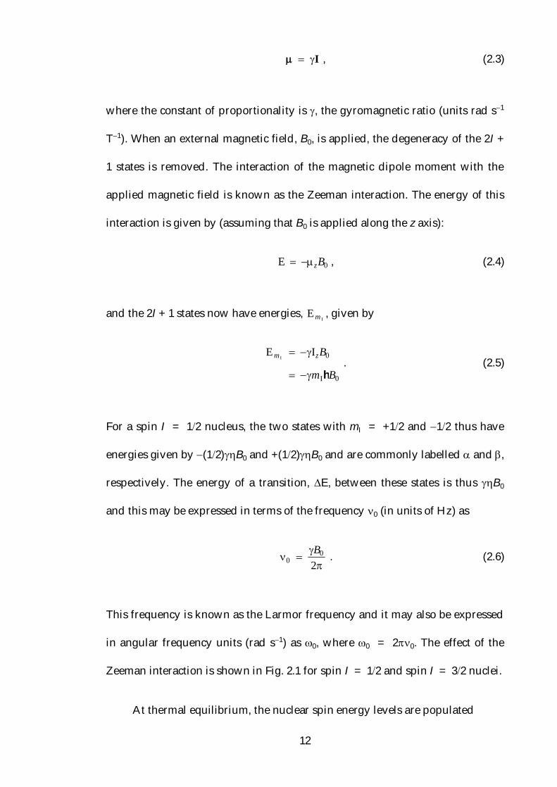
I , (2.3)
where the constant of proportionality is , the gyromagnetic ratio (units rad s1
T1). When an external magnetic field, B0, is applied, the degeneracy of the 2I +
1 states is removed. The interaction of the magnetic dipole moment with the
applied magnetic field is known as the Zeeman interaction. The energy of this
interaction is given by (assuming that B0 is applied along the z axis):
E zB0 , (2.4)
and the 2I + 1 states now have energies, E m I, given by
E m I IzB0
mIh B0
. (2.5)
For a spin I = 12 nucleus, the two states with mI = +12 and 12 thus have
energies given by (12)B0 and +(12)B0 and are commonly labelled and ,
respectively. The energy of a transition, E, between these states is thus B0
and this may be expressed in terms of the frequency 0 (in units of Hz) as
0
B0
2 . (2.6)
This frequency is known as the Larmor frequency and it may also be expressed
in angular frequency units (rad s1) as 0, where 0 = 20. The effect of the
Zeeman interaction is shown in Fig. 2.1 for spin I = 12 and spin I = 32 nuclei.
At thermal equilibrium, the nuclear spin energy levels are populated

13
Figure 2.1. The effect of the Zeeman interaction on the energy levels of (a) a spin I = 12
nucleus and (b) a spin I = 32 nucleus.
according to the Boltzmann distribution, leading to a slight excess of spins in
the lower energy state (assuming > 0). This leads to a greater number of
dipole moments aligned parallel to the field and, consequently, a bulk
magnetization, M, is present in the sample. It is this magnetization which is
manipulated in NMR.
2.2 The Vector Model
Whilst quantum mechanics is required to describe the behaviour of
isolated spin-12 nuclei, classical mechanics may be used to describe the
behaviour of an ensemble of spins that is present in a macroscopic sample. This
may be achieved, at least in the case of simple NMR experiments, by using the
"vector model" [68].

14
The bulk magnetization, M, present in a macroscopic sample at thermal
equilibrium may be conveniently represented by a vector M oriented parallel to
the z axis. When a radiofrequency (rf) pulse is applied, a linearly oscillating B1
field exists in the transverse (xy) plane. This field oscillates at a frequency, rf,
chosen to be close to the Larmor frequency of the spins being observed. In a
static reference frame, known here as the laboratory frame, the B1 field may be
considered to be the sum of two fields, one rotating at a frequency of +rf and
the other at rf. The field rotating at a frequency of rf is far away from the
Larmor frequency of the spins and so its effects may be disregarded. The effect
on the bulk magnetization that results from its interaction with both the B0 and
B1 fields is difficult to visualise in the laboratory frame. Consequently, this
effect is visualised by changing to a coordinate system that is rotating about the
z axis at a frequency rf. In this frame of reference, known as the rotating frame,
the +rf part of the B1 field appears static.
In the rotating frame, the apparent Larmor frequency of precession is
given by = 0 rf, where is known as the offset frequency. Consequently,
the field present along the z axis in the rotating frame, known as the reduced
field, B, is given by
B
. (2.7)
There are thus two orthogonal fields to consider in the rotating frame, B and
B1. Whereas in the laboratory frame the magnetization precesses at its Larmor

15
Figure 2.2. Vector model depiction of (a) the magnetic fields present in the rotating frame and
(b) and (c) the effect of an rf pulse applied about the x axis with B = 0 for the values of
indicated.
frequency about the B0 field, in the rotating frame the magnetization precesses
about the effective field, Beff, which is defined as the resultant of the B and B1
fields and has a magnitude given by:
Beff B 2 B1 2 . (2.8)
The presence of these fields in the rotating frame is depicted in Fig. 2.2a, where
the angle , known as the tilt angle, is given by
tan 1 B1
B
. (2.9)
When viewed in the rotating frame, the effect of a radiofrequency pulse
applied along the x axis is that the magnetization nutates in the yz plane until it
is switched off. The angle through which the magnetization nutates during the
pulse is known as the flip angle, , defined (in radians) as
16
rf , (2.10)
where is the duration of the pulse (in seconds). For an on-resonance pulse,
that is, one for which the offset frequency is zero, the effective field is coincident
with the B1 field ( = 2). In such a case, a pulse applied along the rotating
frame x axis with = 2 will cause a nutation of the magnetization in the yz
plane, onto the y axis, whilst one with = (known as an inversion pulse)
will lead to the magnetization nutating to the z axis. This is illustrated in Figs.
2.2b and 2.2c, respectively.
After a pulse has been applied, the magnetization precesses about the
rotating frame z axis at a frequency (with the exception of an inversion pulse,
which leaves the magnetization vector aligned along the z axis). This
precession does not continue indefinitely, however, and it is damped by
relaxation processes which return the magnetization vector to its orientation at
thermal equilibrium, along the z axis. The loss of magnetization from the xy
plane (the return to its equilibrium value of zero) is known as transverse
relaxation and is quantified by an exponential time constant T2, whilst the
return of the z-magnetization to its equilibrium value is known as longitudinal
relaxation and is described by an exponential time constant T1.
As the magnetization precesses about the z axis a current is induced in a
receiver coil oriented in the xy plane. This decaying current is referred to as the
free induction decay (FID) and it is this which forms the time-domain signal
that is detected in an NMR experiment. The FID is subjected to a Fourier

17
transform, which, as described in the next section, produces a frequency-
domain signal.
2.3 Fourier Transform NMR
The FID acquired in NMR, denoted s(t), typically takes the following form
for a simple one-pulse experiment:
s(t ) C exp( it) exp(t / T2 ) , (2.11)
where C represents the amplitude of the time-domain signal. A single detector
is unable to determine the sense of precession (i.e., the sign of ) in the rotating
frame. To overcome this problem, a method known as quadrature detection is
used [69]. In this method, two datasets are collected for each FID that are 2
radians out of phase with respect to one another. This method yields signals of
the form cos(t) and sin(t); these correspond to the x- and y- (real and
imaginary) components of the transverse magnetization in the rotating frame.
When quadrature detection is used, the FID is sampled at intervals of
seconds, such that, in accordance with the Nyquist theorem [70], the resultant
spectrum covers a frequency range given by SW = 1, where SW is the
spectral width in units of Hz.
A Fourier transform [71, 72] may be used to convert a time-dependent
signal, s(t), into one which is frequency dependent, S(), where

18
S() s(t ) exp( it)d t
0
. (2.12)
This method converts a dataset that is a function of time to one which is a
function of frequency and so, assuming T2 = ∞, produces a frequency-
dependent spectrum that has an amplitude proportional to C when = and
that is zero for all other frequencies.
The FID consists of real and imaginary components and hence, Fourier
transformation of this signal will produce a spectrum that contains real and
imaginary parts. The expression for S() yielded by the Fourier transform of Eq.
(2.12) takes the form
S() C(A() iD()) , (2.13)
where A() and D() consititute the real and imaginary parts of the spectrum
and represent absorptive and dispersive Lorentzian functions, respectively:
A() RR2 ( )2
D() ( )R2 ( )2
, (2.14)
where R = 1T2 is the rate constant for transverse relaxation expressed in units
of Hz. The C factor merely leads to a scaling of the spectrum and so is omitted.
These functions are shown in Fig. 2.3, where the absorptive lineshape shown in
Fig. 2.3a has a peak intensity of 1R and a width at half-height, 12, of 2R rad
s1 (or R Hz), whereas the dispersive lineshape in Fig. 2.3b has an intensity of

19
Figure 2.3. The (a) absorptive and (b) dispersive Lorentzian lineshapes that comprise the real
and imaginary parts of the spectrum obtained by Fourier transformation of a signal acquired
using quadrature detection. The spectral width is 10 kHz and the linewidth at half-height, 12,
is 200 Hz.
12R and a width at half-height of ~7.5 R rad s1. The reduced intensity and
greater breadth of the dispersive lineshape makes it much less desirable in
NMR spectra and so usually only the real part of the spectrum, i.e., that
comprising the absorptive Lorentzian, is shown.
2.4 Density Operator Formalism
The theory of quantum mechanics states that individual spins may be
described by a wavefunction, (t) [73], which can be written as the linear
combination of an orthogonal set of basis functions, n:
(t) cn (t )n
n , (2.15)
where cn(t) are time-dependent coefficients. In a macroscopic sample there are

20
many such spins present and so computing the wavefunction for every spin
quickly becomes rather laborious. Conveniently, there exists a method that
overcomes this difficulty. This uses the density operator, , which is defined as
[74]
(t) (t) , (2.16)
where the overbar indicates an ensemble average. If, for a nucleus with spin I =
12 it is assumed that each spin has a wavefunction that is a superposition of the
and eigenstates in the Zeeman basis set, then (t) and (t ) are given
by:
(t) c (t ) c(t)
(t ) c (t ) c (t) , (2.17)
where c (t) and c
(t) are complex conjugates of the coefficients c(t) and c(t).
An operator Q may be expressed in matrix form using a set of basis
functions such that the element in row i and column j is given by the integral
tdQQ jiij , (2.18)
which may also be written in Dirac notation as
Q ij i Q j . (2.19)
In the case that Q = , the density operator thus has a matrix representation

21
whose elements, ij, are given by:
ij ci(t)cj(t) . (2.20)
The density operator may thus be expressed in matrix form as:
11 12
21 22
. (2.21)
Note that the use of two basis functions yields a 2 2 matrix representation of
the density operator. The diagonal elements, 11 and 22, correspond to the
probabilities of the spins being found in the and states of the Zeeman
Hamiltonian and so simply represent the relative populations of these states.
The off-diagonal elements correspond to coherent superpositions of the and
eigenstates and are termed coherences. At thermal equilibrium, the density
matrix, eq, is directly proportional to Iz, the z-component of the spin angular
momentum operator, and so is given by [74]:
eq Iz
12
0
0 12
. (2.22)
In the case of a spin I = 12 nucleus, the off-diagonal elements correspond to
coherences that have mI = ±1 (they are said to have coherence order p = ±1)
and are the only coherences observed directly in NMR. By convention,

22
however, only p = 1 coherences are observed when quadrature detection is
used. The equilibrium density matrices of nuclei with larger spin quantum
numbers contain off-diagonal elements corresponding to coherences with p >
1. Whilst such coherences are not directly observable in NMR, they form a
crucial part of many experiments, some of which are described in Chapter 3.
In order to obtain the value of an observable, the expectation value of the
corresponding operator, Q, is needed. This is given by
iQjji
iQj)(c)(c)(Q)(Q
i j
i jji
tttt
. (2.23)
This can be shown to be equal to the trace (the sum of the diagonal elements) of
the matrix product of the operator with the density operator:
(t ) Q (t) Tr{Q} . (2.24)
As was described in Section 2.3, the real and imaginary components of the
observed signal in an NMR experiment correspond to the x- and y-components
of the magnetization vector in the rotating frame. These are proportional to Ix
and Iy, the x- and y-components of the spin angular momentum, the matrix
representations of which are given in Appendix A. Consequently, the trace of
the product of with Ix and Iy will yield the real and imaginary components of
the observable signal.

23
To use the density operator to predict the course of an NMR experiment,
its evolution with time needs to be considered. This is achieved using the
Liouville-von Neumann equation [75], which is derived from the time-
dependent Schrödinger equation:
d(t )d t
i H(t ), (t )
i H(t )(t) (t)H(t ) , (2.25)
where (t) is the density operator at time t and H(t) is the Hamiltonian
describing the spin system at time t. If the Hamiltonian is, or can be made to
appear, time-independent then the solution to Eq. (2.25) is given by:
(t) exp iH t (0) exp iH t , (2.26)
where (0) is the value of the density operator at time t = 0. The Hamiltonian
under which the spin system is evolving can be chosen to represent a range of
interactions, such as the resonance offset, chemical shift, and quadrupolar
interactions. The Hamiltonian describing a particular interaction may, like the
density operator, be described in matrix form, and so determining the value of
(t) simply involves the multiplication of three matrices.
Take, for example, the effect of a 2 pulse aligned along the rotating
frame x axis on the equilibrium magnetization of a spin I = 1 nucleus. The
equilibrium density matrix, defined to be the density matrix at time t = 0, is
given by:
24
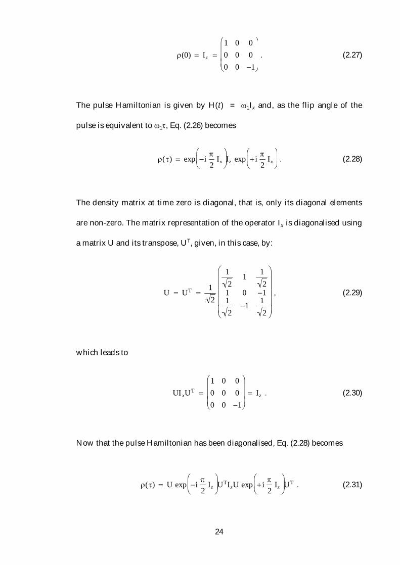
(0) Iz 1 0 00 0 00 0 1
. (2.27)
The pulse Hamiltonian is given by H(t) = 1Ix and, as the flip angle of the
pulse is equivalent to 1, Eq. (2.26) becomes
() exp i
2Ix
Iz exp i
2Ix
. (2.28)
The density matrix at time zero is diagonal, that is, only its diagonal elements
are non-zero. The matrix representation of the operator Ix is diagonalised using
a matrix U and its transpose, UT, given, in this case, by:
U UT 12
12
1 12
1 0 112
1 12
, (2.29)
which leads to
UI xUT 1 0 00 0 00 0 1
Iz . (2.30)
Now that the pulse Hamiltonian has been diagonalised, Eq. (2.28) becomes
() U exp i
2Iz
UTIzU exp i
2Iz
UT . (2.31)

25
The exponential of a diagonal matrix is simply a matrix consisting of the
exponentiated diagonal elements and so it is then a simple matter to arrive at
the solution:
() i2
0 1 01 0 10 1 0
Iy . (2.32)
This result shows that the effect of a 2 pulse aligned along the x axis on the z-
component of the bulk magnetization is to convert it into the y-component of
the magnetization. This is equivalent to a rotation of the bulk magnetization
vector M from the z axis onto the y axis, and so is in accordance with the
vector model description in Section 2.2.
2.5 Tensor Operators
Whilst the density matrix formalism is a convenient way of observing the
effect on the magnetization of, for example, an rf pulse, it can become rather
unwieldy for larger spin quantum numbers, as the density matrix of a single
spin I nucleus (which has dimensions of 2I + 1 2I + 1) quickly increases in size.
This problem may be alleviated by instead expressing the density operator as
the linear combination of a sum of operators, Ai:
(t ) a i (t )A i
i . (2.33)

26
For a pair of spin I = 12 nuclei, operators derived from the products of
Cartesian spin angular momentum operators have been used very successfully
[76]. For quadrupolar nuclei, however, the density operator is commonly
expressed in terms of irreducible spherical tensor operators, Tl,p [77]:
(t ) a l,p(t )Tl,p
p -l
l
l 0
2I , (2.34)
where Tl,p is a spherical tensor of rank l which can take the values 0, 1, 2, ..., 2I
and where p, the coherence order, can take the values l, l + 1, ..., +l. The
matrix representations of these operators are given in Appendix B. T1,0
represents a state with coherence order zero, that is, it describes a population
state [77]. This operator is proportional to the z-component of the spin angular
momentum:
T1,0 Iz . (2.35)
Likewise, the x- and y-components of the spin angular momentum, described
using the angular momentum operators Ix and Iy, may be expressed in terms of
tensor operators of rank 1 and coherence order +1 and 1:
Ix T1,1 T1,1 Iy (T1,1 T1,1)
. (2.36)
The behaviour of tensor operators when evolving under the effects of an
offset frequency , a quadrupolar splitting Q and an rf pulse may be simply

27
expressed. In the presence of an offset, tensor operators evolve for a time
according to [77]
Tl , p Tl , peip , (2.37)
Evolution under an offset thus has the effect of altering neither the rank nor
coherence order of the tensor operator, instead changing the phase. In many
modern experiments the effect of the offset can be ignored as the presence of a
pulse refocuses the chemical shift interaction.
Under the influence of a pulse, tensor operators evolve according to [77]
Tl , p
(Iy cos Ix sin ) Tl , p
p d p ,p
l ()eip , (2.38)
where is the flip angle of the pulse, is the phase of the pulse (zero for a pulse
aligned along the y axis), and p p p is the change in coherence order.
Reduced Wigner rotation matrix elements are represented by d p , pl () and their
values may be found in Appendix C for l = 1, 2 and 4. Eq. (2.38) reveals that a
pulse changes the coherence order, but not the rank, of a tensor operator.
Consider, for example, the effect on the z-magnetization of a 2 pulse aligned
along the rotating frame y axis. The z-magnetization, described by the tensor
operator T1,0, evolves as follows:
T1,0
( / 2)y 12
{T1,1 T1,1} . (2.39)

28
The combination of tensor operators of rank 1 and coherence order +1 and 1 is
proportional to the x-component of the spin angular momentum, Ix. This result
thus agrees with that predicted by the vector model.
In the presence of a first-order quadrupolar interaction, tensor operators
evolve in the following way for a time, :
I
l lpl
pl,lpl
2,
Q, T)(cT , (2.40)
where Q is the quadrupolar splitting parameter and the values of the
coefficients c l ,lp () are given in Appendix D. Free precession in the presence of a
quadrupolar interaction thus changes the rank, but not the coherence order, of a
tensor operator. It is the combination of this evolution and that under an rf
pulse that can lead to the creation of multiple-quantum coherences. In the case
of triple-quantum coherence, the operators T3,1, T3,+1, T3, 3 and T3,+3 are created
and are present (with the exception of T3,1 and T3,+1, which are removed by
phase cycling) during the t1 period of the triple-quantum MAS experiment
described in Chapter 3.
Using the tensor operator formalism, it is thus easy to show the effect of a
pulse and of evolution under a quadrupolar splitting or offset. The well-defined
behaviour of tensor operators under these conditions provides a convenient
way in which to consider the effects of the more complex NMR experiments for
which a vector model description is inadequate.

29
2.6 Line Broadening Mechanisms
There exist several mechanisms that can lead to line broadening in NMR
spectra in the solid state. Two of the most significant, the chemical shift and
dipolar coupling, are introduced in this section and their effect on solid-state
NMR spectra is described. Another major source of line broadening in the case
of quadrupolar nuclei is the quadrupolar interaction. This will be described in
detail in Chapter 3.
2.6.1 Chemical Shift
When a magnetic field is applied, electrons begin a circulatory motion
about a nucleus. This motion creates a magnetic field that can either increase or
decrease the magnetic field experienced by the nucleus. This shielding is the
origin of the chemical shift and has the effect of modifying the Larmor
frequency defined in Eq. (2.6) to [78]:
0 B0 (1 ) . (2.41)
In Eq. (2.41), is the chemical shielding tensor. The chemical shielding has
the properties of a second-rank Cartesian tensor and as such may be
represented by a 3 3 matrix. This is also the case for the dipolar interaction
(described in Section 2.6.2) and the first-order quadrupolar interaction
(described in Chapter 3) and in each case, the tensor is defined with respect to a
frame of reference such that this matrix is diagonal. This reference frame is

30
known as the principal axis system (PAS). In such a reference frame, the tensor
is defined by three quantities, referred to as the principal values describing the
interaction. For chemical shielding, these are defined as XXPAS , YY
PAS and ZZPAS
and correspond to the principal values of the interaction associated with the
PAS X, Y and Z axes, respectively. The chemical shielding tensor may thus be
represented by the following matrix in its PAS:
XX
PAS 0 00 YY
PAS 00 0 ZZ
PAS
, (2.42)
where these principal values may be used to define an isotropic value of the
chemical shielding tensor, iso, an anisotropy, , and an asymmetry, :
iso 13
XXPAS YY
PAS ZZPAS
ZZPAS iso
XX
PAS YYPAS
. (2.43)
In NMR, absolute frequencies are not measured; instead, frequencies are
quoted as chemical shifts with respect to a reference material. The chemical
shift, iso, is thus defined as follows [79]:
iso
0 0 (ref )0 (ref )
iso (ref ) iso
1 iso (ref ) , (2.44)

31
where 0(ref) and iso(ref) are the Larmor frequency and isotropic value of the
chemical shielding tensor of the reference sample, respectively. The chemical
shift, defined in Eq. (2.44), also has the properties of a second-rank Cartesian
tensor and as such may be defined by three principal values in its PAS, PASXX ,
PASYY and PAS
ZZ . Using these principal values, the isotropic chemical shift, iso,
the chemical shift anisotropy, CS, and the chemical shift asymmetry, CS, are
defined as
CS
PASYY
PASXX
CS
isoPASZZCS
PASZZ
PASYY
PASXXiso 3
1
. (2.46)
The observed chemical shift, , is defined as the sum of isotropic and
anisotropic contributions:
iso
12cs {3 cos2 1 cs sin 2 cos 2} , (2.47)
where and are polar angles that define the orientation of the B0 field in the
PAS of the chemical shielding tensor. In the solution state, rapid molecular
tumbling averages the anisotropic component of the chemical shift to zero and
so only the isotropic component is observed. In the solid state, however, the
general lack of motion means that the anisotropic component of the chemical
shift is no longer averaged to zero. This means that, due to the range of
orientations observed in a powder, each crystallite has a different chemical shift

32
and so a ''powder pattern'' is observed in the spectrum.
2.6.2 Dipolar Coupling
There exists an interaction between the magnetic moments of nuclei that
are close in space. This through-space interaction is referred to as the dipolar
interaction and, for the case of a homonuclear IS spin pair, is defined by the
following first-order average Hamiltonian, H ddhom , expressed in the rotating
frame [80]:
H ddhom D(3IzSz I S) , (2.48)
where I S = IxSx + IySy + IzSz and D is the dipolar coupling parameter, given
by:
D
DPAS
23 cos2 1 , (2.49)
where is the angle between the I-S internuclear vector and B0. DPAS is the
dipolar coupling parameter in the principal axis system of the dipolar coupling
tensor and is defined as [81, 82]:
D
PAS 0ISh
4rIS3 , (2.50)
with I and S being the gyromagnetic ratios of the I and S spins and rIS their
internuclear distance.

33
Like the chemical shielding interaction described in Section 2.6.1, the
dipolar coupling has the properties of a second-rank Cartesian tensor. In
contrast to the chemical shielding, however, the dipolar coupling tensor is
traceless and so its isotropic value, Diso, is zero. In addition, the dipolar
coupling tensor is always axially symmetric ( = 0).
In the solution state, the presence of molecular motion averages the
dipolar coupling to its isotropic value. This means that, if residual linewidths
are ignored, no evidence of the presence of the dipolar coupling is seen in the
spectrum. In the solid state, however, the general lack of motion means that the
averaging seen in the solution state is not observed. The angular dependence of
D means that, in a powdered solid, a range of dipolar couplings exists, so
producing a powder pattern in the NMR spectrum.
As shown in Eq. (2.50), the strength of the dipolar interaction between two
nuclei I and S is proportional to IS. The effect of the Hamiltonian in a multi-
spin homonuclear system is to remove the degeneracy of the many Zeeman
levels that have the same net azimuthal quantum number. This arises because
of the homogeneous nature of this interaction [11] and leads to a very large
range of transition frequencies in the NMR spectrum of such a spin system. For
homonuclear dipolar couplings between nuclei such as 1H and 19F, this means
that the resultant spectra commonly contain linewidths of up to 30kHz.
The dipolar interaction between two non-equivalent spin species I and S is
characterised by the following first-order rotating frame average Hamiltonian:
34
zzmm SI2H SIDhetdd . (2.51)
If the I and S spins are assumed to be spin I = 12 nuclei, then this has the effect
of shifting the energies of the four Zeeman levels by ±D2. The two transitions
of each of the I and S spins, that have equal frequencies in the absence of a
dipolar coupling, are thus shifted by ±D. The orientational dependence of D
leads to a powder pattern in the spectrum, and as the dipolar coupling has, like
the chemical shift, the properties of a second-rank Cartesian tensor, this powder
pattern consists of two overlapping axially symmetric CSA patterns (one for
each transition) that are mirror images of one another. Line broadening due to
heteronuclear dipolar coupling can be removed by, in addition to MAS [37], a
technique known as decoupling [25]. This involves applying high-power
continuous irradiation at the Larmor frequency of the spin that is being
decoupled (typically the S spin). This causes rapid transitions between the S-
spin Zeeman states such that the observed (I) spin transitions are once again
degenerate and a single peak at the I-spin frequency, from which anisotropic
line broadening due to the dipolar interaction has been removed, is observed.
2.7 Two-Dimensional NMR
Many routine NMR experiments are two-dimensional in nature. They
differ from their one-dimensional counterparts in that they comprise two time
periods during which the magnetization evolves, conventionally labelled t1 and
t2. The typical form of a two-dimensional NMR experiment [83, 84] is shown in

35
Fig. 2.4.
An initial pulse of phase 1 excites transverse magnetization that is then
allowed to evolve during the t1 period. Another pulse (or commonly, a
sequence of pulses) of phase 2 then converts this magnetization to p = 1
central-transition coherence that is detected during the t2 period. This process is
typically repeated 64–256 times, with the t1 period being incremented each time.
This yields a time-domain signal, s(t1, t2), that is a function of two time
periods, and that commonly (though not always) is cosine modulated during
the t1 period:
s(t1 , t2 ) cos 1t1 exp(R1t1) exp( i2t2 ) exp( R2t2 ) , (2.52)
where R1 and R2 are transverse relaxation rate constants during the t1 and t2
periods, respectively. Performing a Fourier transformation in both dimensions
then yields a two-dimensional spectrum that, like its one-dimensional
analogue, contains real and imaginary components. The two dimensions, 2
and 1, are known as the direct and indirect dimensions, respectively. For two-
dimensional experiments to be useful, it is a necessity that the real part of the
spectrum contains lineshapes that are purely absorptive in both dimensions;
that is, they contain none of the highly undesirable dispersive character that
was described in Section 2.3.

36
Figure 2.4. The typical form of a two-dimensional NMR experiment. The t1 period is
incremented in successive one-dimensional experiments such that a signal is produced in which
the magnetization has evolved during two time periods.
2.7.1 Phase Modulation
In Section 2.3 it was shown how the Fourier transform converts a dataset
that is a function of time to one which is a function of frequency:
s(t ) FT S() , (2.53)
where S() may be expressed as the sum of its absorptive and dispersive
Lorentzian components:
S() A() iD() . (2.54)

37
Figure 2.5. Pulse sequence and coherence transfer pathway for the N-type COSY experiment.
Consider, for example, a simple two-pulse N-type COSY experiment [85].
The coherence transfer pathway and pulse sequence for this experiment are
shown in Fig. 2.5. As is now customary for many modern two-dimensional
experiments, phase cycling is used to ensure the correct coherence transfer
pathway is selected [86, 87]. A two-dimensional experiment of this form, in
which only one coherence transfer pathway is selected during the t1 period,
yields a time-domain signal of the form:
s(t1 , t2 ) exp(i1t1) exp(R1t1) exp( i2t2 ) exp(R2t2 ) . (2.55)
A function of the form exp(it) is not an even function, that is, exp(it) ≠
exp(it). Consequently, a time-domain dataset of the form in Eq. (2.55) is
sensitive to the sign of the offset and is said to be frequency discriminated.
Fourier transformation in the t2 dimension leads to the following dataset:
s(t1 , 2 ) exp(i1t1) exp(R1t1){A(2 ) iD (2 )} . (2.56)
Inspection of the spectrum obtained in the 2 dimension reveals that the phase
38
of the lineshape varies as a function of t1. Two-dimensional experiments
producing time-domain data in the form of Eq. (2.55) are thus said to be phase
modulated.
A second Fourier transformation, in the t1 dimension, leads to the two-
dimensional dataset
S(1 , 2 ) {A(1) iD(1)}{A(2 ) iD(2 )}
[A(1)A(2 ) D(1)D(2 )]
i[D(1)A(2 ) A(1)D(2 )]
. (2.57)
Equation (2.57) reveals that the real part of the spectrum contains a mixture of
doubly-absorptive and doubly-dispersive contributions. The lineshape arising
from such contributions is known as a phase-twist lineshape, and, on account of
it having both positive and negative parts, it is thus unsuitable for high-
resolution NMR. Performing an experiment in which p = 1 coherences are
selected during the t1 period (known as a P-type COSY experiment [85])
produces a time-domain signal, which, after Fourier transformation in both
dimensions, yields a dataset that differs from that in Eq. (2.57) only in the sign
of the frequency in the 1 dimension. Phase-modulated experiments thus
achieve the desired frequency discrimination, but have the undesirable by-
product of a phase-twist lineshape.

39
2.7.2 Amplitude Modulation
Many two-dimensional NMR experiments involve the selection of more
than one coherence transfer pathway during the t1 period. An example of this is
the double-quantum filtered (DQF)-COSY experiment [88], the pulse sequence
of which is shown in Fig. 2.6. Experiments such as this yield a time-domain
signal of the form
s(t1 , t2 ) 12
{exp(i1t1) exp( i1t1)}
exp( R1t1) exp( i2t2 ) exp( R2t2 )
cos(1t1) exp( R1t1) exp( i2t2 ) exp( R2t2 )
. (2.58)
Such a signal is said to be amplitude modulated, as variation of t1 modifies only
its amplitude, and not its phase. The Fourier transform of a function of the form
cos(t)exp(Rt) (a cosine Fourier transform) yields an absorptive Lorentzian,
A(). The resulting spectrum thus contains, in contrast to the Fourier transform
of a complex exponential function, only real components. Consequently, a two-
dimensional Fourier transform of the time-domain signal in Eq. (2.58) yields a
dataset of the form:
S(1 , 2 ) A(1){A(2 ) iD(2 )} . (2.59)
The real part of this signal is of the form A(1)A(2) and so yields a doubly-
absorptive lineshape. Amplitude-modulated experiments thus produce spectra
containing not the phase-twist lineshapes observed with phase-modulated
experiments, but lineshapes whose doubly-absorptive nature makes them far

40
Figure 2.6. Pulse sequence and coherence transfer pathway for the DQF-COSY experiment.
more conducive to high-resolution NMR. However, amplitude-modulated data
lack the frequency discrimination possessed by phase-modulated data. This is a
direct consequence of the relations
cos(1t1) cos(1t1)
sin(1t1) sin( 1t1) . (2.60)
This lack of frequency discrimination is a drawback of acquiring amplitude-
modulated data. The following section describes methods that allow both
frequency discrimination to be achieved and doubly-absorptive lineshapes to
be obtained.
2.7.3 States-Haberkorn-Ruben and TPPI Methods
A phase shift of 2 radians of a cosine function yields a sine function. The
States-Haberkorn-Ruben (SHR) method [89] achieves frequency discrimination

41
by using both cosine- and sine-modulated time-domain signals. When a Fourier
transform is performed in the t2 dimension, time-domain signals that have sine
and cosine modulation in t1, denoted Ssin(t1, 2) and Scos(t1, 2) respectively, are
obtained:
Scos (t1 , 2 ) cos(1t1) exp( R1t1){A 2 ) iD(2 }Ssin (t1 , 2 ) sin(1t1) exp( R1t1){A(2 ) iD(2 )}
. (2.61)
In the SHR method, a new dataset is formed, SSHR(t1, 2), in which the real
and imaginary components are the real parts of the cosine- and sine-modulated
datasets, respectively:
)(A)Rexp()sin(i
)(A)Rexp()cos(),(S
21111
2111121SHR
tt
ttt . (2.62)
This may also be expressed as:
SSHR (t1 , 2 ) exp( i1t1) exp(R1t1)A(2 ) , (2.63)
which, after Fourier transformation in the indirect dimension gives:
SSHR (1 , 2 ) {A(1) iD (1)}A(2 )
A(1)A(2 ) iD(1)A(2 ) . (2.64)
The real part of this signal is doubly absorptive and so is of the required form
for high-resolution two-dimensional NMR.
There exists an alternative technique for achieving frequency
42
discrimination, known as time proportional phase incrementation (TPPI) [90].
This method is similar to the SHR method and operates by shifting the phase of
the pulse, or group of pulses, that preceed the t1 period, for each increment of t1.
This phase shift, equal to (2p), where p is the order of coherence evolving
during the t1 period, leads to the following dataset, after Fourier transformation
in the t2 dimension:
)(A)Rexp())2/)(2((cos),(S 21111121TPPI ttSWt , (2.65)
where 1SW1 is equal to the t1 increment. In this method, the spectral width in
the 1 dimension is doubled and so, in accordance with the Nyquist theorem,
the sampling interval in the indirect dimension (the t1 increment) is halved.

43
Chapter 3
Quadrupolar Interaction
3.1 Introduction
The dominant interaction for nuclei with spin I > 12 is usually that
which arises between the nuclear electric quadrupole moment and the electric
field gradient [91–93]. This quadrupolar coupling commonly has a magnitude
of the order of megahertz and is responsible for the large quadrupolar splittings
observed in solid-state NMR spectra of quadrupolar nuclei. In liquids, the
quadrupolar interaction is also responsible for efficient quadrupolar relaxation.
The major source of line broadening for quadrupolar nuclei is the
inhomogeneous contribution arising from the quadrupolar coupling and it is
this which determines the appearance of the resultant NMR spectra in the solid
state. In this section, the origin of this quadrupolar broadening will be
described, as will the equations describing its effects and the implications for
the appearance of the spectra.
3.2 The Quadrupolar Coupling
In addition to the magnetic dipole moment that is characteristic of all
NMR-active nuclei, nuclei with spin I 12 possess an electric quadrupole

44
moment, eQ. The electric quadrupole moment takes a fixed value and is
characteristic of the nucleus. The presence of a non-spherical distribution of
electrons around a nucleus leads to an electric field gradient (EFG). The electric
field gradient is a three-dimensional entity which can be described using the
EFG tensor, V. This tensor can be described by three components in its PAS.
These are denoted VXXPAS , VYY
PAS and VZZPAS and correspond to the principal values
of the electric field gradient associated with the X, Y and Z PAS axes,
respectively. These components satisfy the conditions
PASYY
PASXX
PASZZ
PASZZ
PASYY
PASXX
VVV
0VVV
. (3.1)
The EFG tensor is traceless and so its isotropic value is zero. This means
that its anisotropy is equal to VZZPAS and so is given by eq, where e is the
magnitude of the electron charge. The coupling of the quadrupole moment (eQ)
and the EFG (eq) leads to an interaction that is quantified, in units of Hertz,
using a quadrupolar coupling parameter CQ [94]:
CQ
e2qQh
, (3.2)
and the cross-sectional shape of the EFG tensor parallel to the XPASYPAS plane is
characterised by an asymmetry parameter, , which can take values between 0
and 1, and is given by:
45
VXXPAS VYY
PAS
VZZPAS . (3.3)
3.3 The Quadrupolar Interaction
3.3.1 The First-Order Quadrupolar Interaction
The Hamiltonian describing a quadrupolar nucleus can be expressed,
neglecting the effects of CSA and any homonuclear and heteronuclear dipolar
couplings, as follows:
H H Z H Q , (3.4)
where the Hamiltonian HZ (equal to 0Iz) expresses the effect of the Zeeman
interaction and HQ that of the quadrupolar interaction. Whilst the quadrupolar
interaction can in some cases be very large, it is typically at least an order of
magnitude smaller than the Zeeman interaction. This means that its effect on
the energy levels can be considered as a perturbation of the dominant Zeeman
term and so time-independent perturbation theory may be used [95]. The
quadrupolar Hamiltonian is given by the following equation, expressed in the
PAS of the EFG tensor [96]:
H Q
PAS QPAS IZ
2 13
I I 1 3
IX2 IY
2
, (3.5)
where IX, IY and IZ are analogous to the operators Ix, Iy and Iz defined in Chapter

46
2. QPAS is defined as the magnitude of the quadrupolar interaction in the PAS
of the EFG tensor and is given, in units of rad s1, by
Q
PAS 3CQ
2I(2I 1) . (3.6)
In the laboratory frame, a quadrupolar splitting parameter, Q, is defined, in
units of rad s1:
Q
QPAS
2(3 cos2 1 sin 2 cos 2) , (3.7)
where and are angles relating the PAS of the EFG tensor to B0. Equation (3.7)
reveals the quadrupolar splitting to be orientationally dependent. For a
powdered solid, this means that each crystallite orientation will experience a
different quadrupolar splitting, so giving rise to a powder pattern.
Equation (3.5) may also be expressed using spherical tensor operators (for
a spin I = 32 nucleus) as:
H Q
PAS 2QPAS T2 ,0
6
T2 ,2 T2,2
, (3.8)
or in matrix form as:

47
H QPAS Q
PAS
1 0 3
0
0 1 0 3
3
0 1 0
0 3
0 1
. (3.9)
To determine the effects of the quadrupolar interaction, the Hamiltonian
must first be transformed to the laboratory frame. As tensor operators have
well-defined properties under rotation, the quadrupolar Hamiltonian defined
in Eq. (3.8) is used. A tensor of rank l and coherence order p, denoted Tl,p,
transforms from one frame of reference to another via a rotation R(, , ) as
[97]:
R(, , )Tl,pR1( , , ) D p , p
l , , p l
l Tl, p , (3.10)
where , and are the Euler angles [98] that relate the two frames of reference
and R1(, , ) is the inverse of the rotation operator R(, , ). The Euler
angles, , and , are defined as rotations of about the laboratory frame x
axis, of about the laboratory frame y axis and of about the laboratory frame z
axis, respectively. D p ,pl (, , ) are Wigner rotation matrix elements and are
defined as [99]
)}(iexp{)(d),,(D pplp,p
lp,p , (3.11)
where d p , pl () are reduced rotation matrix elements [100]. Consequently, in the

48
laboratory frame the quadrupolar Hamiltonian, HQ, is expressed as:
H Q 2QPAS [
p 2
2 (D p ,0
2 ( , , ) 6
{D p ,22 (, , )
D p ,22 ( , , )}]T2, p
, (3.12)
which may also be expressed in matrix form:
H Q 2QPAS
A B C 0B A 0 C
C 0 A B
0 C B A
, (3.13)
where
A 12
D002 (, , )
2 6(D0,2
2 (, , ) D0,22 (, , ))
B 12
D1,02 (, , )
12D1,2
2 (, , ) D1,22 (, , )
B 12
D1,02 (, , )
12D1,2
2 (, , ) D1,22 (, , )
C 12
D2 ,02 (, , )
12D2,2
2 ( , , ) D2 ,22 ( , , )
C 12
D2 ,02 (, , )
12D2,2
2 (, , ) D2,22 (, , )
. (3.14)
The first-order perturbation to an energy level, E m I
(1) , is given by [95]
E m I
(1) mI HQ mI . (3.15)
Hence, taking the example of the energy level with mI = 32, this is equivalent

49
Figure 3.1. The first-order perturbation to the energy levels of a spin (a) I = 1 and (b) I = 32
nucleus by the quadrupolar interaction.
to the element in the first row and first column (i.e., the first diagonal element)
in the matrix representation of the quadrupolar Hamiltonian. The four Zeeman
states of a spin I = 32 nucleus are thus perturbed as follows:
E3 / 2(1) E3 / 2
(1) Q
PAS
23 cos2 1 Q
E1/ 2(1) E1 / 2
(1) Q
PAS
23 cos2 1 Q
, (3.16)
The first-order perturbation to the energies of the Zeeman states is shown in
Figs. 3.1a and 3.1b for the case of spin I = 1 and spin I = 32 nuclei,
respectively.
Figure 3.1 reveals that, for a spin I = 1 nucleus, the frequency of the (mI =
+1 1) transition (the double-quantum (DQ) transition) is unaffected to first

50
order by the quadrupolar interaction. For a spin I = 32 nucleus, the
frequencies of the (mI = +12 12) and (mI = +32 32) transitions,
known as the central (CT) and triple-quantum (TQ) transitions respectively, are
unaffected to first order. In general, all symmetric transitions are unperturbed
by the first-order quadrupolar interaction. Figure 3.1b shows that for a spin I =
32 nucleus, the frequencies of the (mI = +32 +12) and (mI = 12 32)
transitions, the so-called satellite transitions (ST), are given by 0 2Q and 0
+ 2Q, respectively. For half-integer nuclei with spin I > 32, there is more than
one set of satellite transitions and these are labelled ST1 (the mI = ±32 ±12
transitions), ST2 (the mI = ±52 ±32 transitions), and so on. The orientational
dependence of Q means that, in a powdered solid, a powder pattern is
observed in the NMR spectrum. The absence of an isotropic component in Eq.
(3.16) means that the powder pattern remains centred about 0. Owing to the
absence of a first-order perturbation to the frequency of the central transition,
the resultant powder pattern features a narrow line and it is for this reason that
much solid-state NMR of quadrupolar nuclei has focussed on observation of
solely this transition. The central transition is, however, affected by a smaller
second-order perturbation and so the magnitude of this effect needs to be
determined.
3.3.2 The Second-Order Quadrupolar Interaction
Time-independent perturbation theory states that the second-order
51
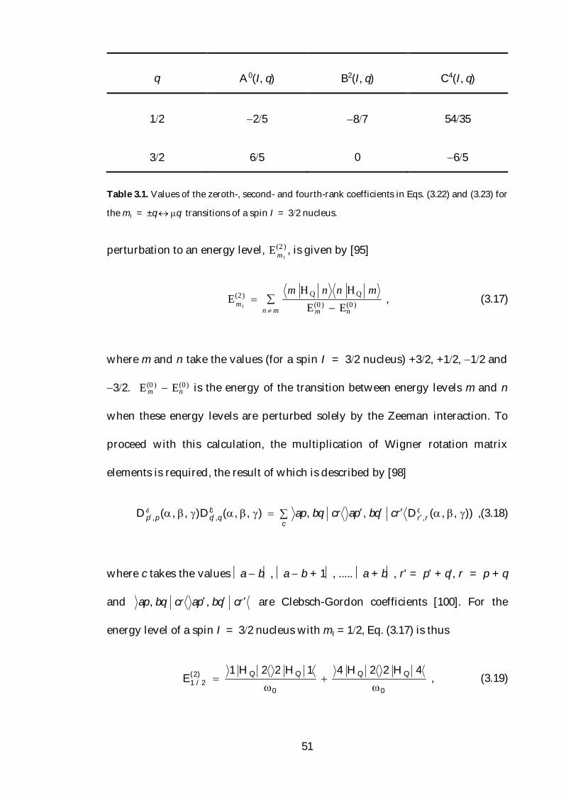
Table 3.1. Values of the zeroth-, second- and fourth-rank coefficients in Eqs. (3.22) and (3.23) for
the mI = ±q q transitions of a spin I = 32 nucleus.
perturbation to an energy level, E m I
(2 ) , is given by [95]
E m I
(2) m H Q n n HQ m
E m(0 ) En
(0 )n m , (3.17)
where m and n take the values (for a spin I = 32 nucleus) +32, +12, 12 and
32. E m(0 ) En
(0) is the energy of the transition between energy levels m and n
when these energy levels are perturbed solely by the Zeeman interaction. To
proceed with this calculation, the multiplication of Wigner rotation matrix
elements is required, the result of which is described by [98]
)),,(D,,),,(D),,(D ,,, c
crr
bqq
app rcqbpacrbqap ,(3.18)
where c takes the values a b, a b + 1, ..... a + b, r' = p' + q', r = p + q
and rcqbpacrbqap ,, are Clebsch-Gordon coefficients [100]. For the
energy level of a spin I = 32 nucleus with mI = 12, Eq. (3.17) is thus
0
0
QQ)2(2/1
4H22H41H22H1E
, (3.19)
q A0(I, q) B2(I, q) C4(I, q)
12
32
25
65
87
0
5435
65
52
which is equal to
E1 / 2
(2) BB
0
CC
0 . (3.20)
Using Eq. (3.18) this can be shown to be equal to
E1 / 2
(2) (Q
PAS )2
20
25
87
D0 ,02 (, , ) 54
35D0 ,0
4 (, , )
, (3.21)
which may be expressed more generally as:
E m I
(2) (Q
PAS )2
20A0 (I, q)Q0 () B2 (I , q)Q2 (, , , )
C4 (I , q)Q4 (, , , ) , (3.22)
and consequently, the second-order perturbation to the frequency of a
transition mI mI is given by
E m I m I
(2) (Q
PAS )2
0A0 (I , q )Q0 ()
B2 (I , q)Q2 (, , , ) C4 (I, q)Q4 (, , , ) , (3.23)
where

53
Figure 3.2. The energy levels of a spin I = 32 nucleus when successively perturbed by the (a)
Zeeman, (b) first-order quadrupolar and (c) second-order quadrupolar interactions.
Q0 () 1 2
3
Q2 (, , , ) 1 2
3
D0 ,0
2 (, , ) 23{D0 ,2
2 (, , )
Q4 (, , , ) 1 2
18
D0 ,0
4 (, , ) 106
{D0 ,24 (, , )
D0,24 (, , )} 35
18 70{D0,4
4 (, , ) D0 ,44 (, , )}
, (3.24)
and A0(I, q), B2(I, q) and C4(I, q) are zeroth-, second- and fourth-rank coefficients
that depend on I and mI. The values of these coefficients for the central and
satellite transitions of a spin I = 32 nucleus are shown in Table 3.1; a complete
listing of these coefficients for spin I = 32 and spin I = 52 nuclei is given in
Appendix E. It should be noted that, as a consequence of Eq. (3.11) and the fact

54
that all the Wigner rotation matrix elements, D p ,pl (, , ) , in Eq. (3.24) have p'
= 0, only the and angles are required to describe the rotation of the PAS of
the EFG tensor into the laboratory frame. If the further simplification that the
asymmetry parameter = 0, is made, then only Wigner rotation matrrix
elements with p = 0 are needed and so only the angle is required.
The effect of the quadrupolar interaction on the energy levels of a spin I =
32 nucleus is shown in Fig. 3.2. Figure 3.2 shows that the central transition
experiences a second-order perturbation (proportional to ( PASQ )20) that is
considerably smaller than the first-order interaction (proportional to QPAS ) that
affects the satellite transitions.
3.3.3 Effect of Sample Spinning
The expressions derived in Sections 3.3.1 and 3.3.2 that describe the
perturbations arising from the first- and second-order quadrupolar interactions
are applicable under "static" (non-spinning) conditions. It has been well
documented that magic angle spinning (MAS) is able to considerably reduce
the anisotropic broadening present in solid-state NMR spectra of quadrupolar
nuclei [8–10]. This leads to improved resolution and so facilitates spectral
interpretation when there are overlapping powder patterns from inequivalent
sites present. In this section, the origin of the line-narrowing effect of MAS is
shown. The implications of MAS for the perturbation of the energy levels is
described and the way that these effects manifest themselves in second-order
55
quadrupolar broadened MAS spectra is considered.
In deriving Eq. (3.12), the quadrupolar Hamiltonian in the laboratory
frame, transformation of the Hamiltonian between two frames of reference was
required. This transformation, from the PAS of the EFG tensor to the laboratory
frame, needed just a single set of Euler angles, , and . Under conditions of
sample spinning, the transformation proceeds via an intermediate frame of
reference, known as the rotor-fixed frame. In this frame of reference, the z axis
is coincident with the sample rotation axis. Two sets of angles are thus required
to define the rotation from the PAS of the EFG tensor to the laboratory frame:
Lab),,0(RRotor),,(RPAS R t , (3.25)
where ', ' and ' are angles relating the PAS of the EFG tensor to the rotor-
fixed frame, and (Rt + ) and are the angles describing the rotation of the
rotor frame onto the laboratory frame, where is the angle between the
spinning axis and B0 and indicates the crystallite orientation relative to the
rotor axis at time t = 0. R is the spinning frequency (in units of rad s1), which
may also be expressed in units of Hertz as R, where R = R2. The
transformation from the rotor-fixed frame to the laboratory frame is seen to
require only 2 angles, which is due to the same reason as in the case of the static
second-order quadrupolar interaction described at the end of the previous
section. By splitting the transformation from the PAS to the laboratory frame of
reference into two rotations, the Wigner rotation matrix elements given in Eq.

56
(3.24), D0, rc (, , ) , are modified to
c
cm
crm
cm
cr t ),,(D),,0(D),,(D ,R,0,0 , (3.26)
where c = 2 or 4. Sample spinning has thus introduced a time dependence that
conflicts with the time-independent perturbation theory that was used in the
previous sections. However, this theory remains valid if an integer number of
rotor periods is assumed. Using Eq. (3.11), the Wigner rotation matrix elements
D0, mc (0, , Rt ) may be written as
D0, mc (0, , Rt ) d 0 , m
c () exp( imRt) exp( im) . (3.27)
The presence of Wigner rotation matrix elements with p' = 0 means that, as in
the case described in the previous section, only two angles are required for the
transformation from the rotor-fixed frame to the laboratory frame. Over the
course of an integer number of rotor periods, t will vary from 0 to (2nR) s,
where n is the number of rotor periods, and under such conditions, the integral
of the term exp(imRt) is only non-zero when m = 0. Consequently, only
Wigner rotation matrix elements of the form D0,0c (0, , Rt ) and
),,(D ,0 cr are required and so Eq. (3.26) may be simplified to
),,(D)(d),,(D 00,0,0 cr,
ccr , (3.28)
and in so doing is made time-independent. Assuming an integer number of
rotor periods, Eq. (3.23) thus becomes:
57
E m I m I
(2 ) (Q
PAS )2
0A0 (I , q )Q0 () B2 (I , q)d 0 ,0
2 ()Q2 ( , , )
C4 (I , q)d 0 ,04 ()Q4 ( , , )
, (3.29)
where
Q0 () 1 2
3
Q2 ( , , ) 1 2
3
d 0,0
2 ( ) 83d 2 ,0
2 ( ) cos 2
Q4 ( , , ) 1 2
18
d 0,0
4 ( ) 103
d 2,04 ( ) cos 4
359 70
2d 4,04 ( ) cos 4
. (3.30)
Notice that the second- and fourth-rank contributions in Eq. (3.29) are
independent of '. If the assumption of axial symmetry is made, then the angle
' is no longer required.
The dependence of the reduced rotation elements in Eq. (3.30) on is
given by
d 0,0
2 () 12
3 cos2 1 , (3.31)
and
d 0,0
4 () 18
35 cos4 30 cos2 1 . (3.32)

58
These elements equal zero when = 54.74° in Eq. (3.31) and 30.56° or 70.12° in
Eq. (3.32). This means that spinning at the magic angle completely removes the
second-rank contribution to the anisotropic broadening, but only reduces the
fourth-rank contribution. The absence of a common root to the equation
d 0 ,0l () 0 , (3.33)
for the cases of l = 2 and l = 4 means that spinning about a single angle is
incapable of removing both second- and fourth-rank anisotropic broadenings.
3.3.4 Second-Order Quadrupolar Broadened Spectra
Inspection of Eq. (3.29) reveals that the second-order perturbation to the
frequency of the transitions of a quadrupolar nucleus contains both isotropic
and anisotropic components. The zeroth-rank component, A0(I, q)Q0(), leads to
an isotropic shift in the spectrum, whilst the second- and fourth-rank
anisotropic terms, B2(I, q)Q2(, , ) and C4(I, q)Q4(, , ), are responsible for
anisotropic line broadening. Figure 3.3 shows simulated central-transition
lineshapes under MAS conditions for a spin I = 32 nucleus, simulated with
= 0, 0.5 and 1, respectively. The orientationally dependent second- and fourth-
rank terms in Eq. (3.29) lead to the observed broadening and the effect of the
zeroth-rank term is evident in the shift of the powder pattern (in this case to
lower frequency) from the centre of the spectrum.

59
Figure 3.3. Computer-simulated MAS second-order quadrupolar central-transition lineshapes
of a spin I = 32 nucleus, simulated using = (a) 0, (b) 0.5 and (c) 1, respectively. The
quadrupolar coupling parameter CQ = 2 MHz, the Larmor frequency is 100 MHz and the
spectra were generated by averaging over 5760 values of the angles and The MAS rate is 40
kHz.
3.3.5 Spinning Sidebands
The assumption made in Section 3.3.3 was that sampling over an integer
number of rotor periods and spinning at the magic angle leads to complete
removal of second-rank anisotropic broadening. This method of data sampling,
in which the free induction decay is sampled at the start of every rotor period,
("rotor-synchronization"), is not the usual method of data acquisition in NMR.
Consequently, the time dependence of the rotation matrix elements given in Eq.
(3.26) needs to be considered. If axial symmetry is assumed, then only the
elements with r = 0 are required and so Eq. (3.23) becomes:
),,0(D
),,0(D),(C),,0(D
)t,,0(D),(B),(A)(
E
20,
4
4R
2,0
420,
2
2R
2,0
20
0
2PAS)2( Q
II
m
mmm
mmmm
tqI
qIqI
, (3.34)

60
where the following relations have been used for deriving the second- and
fourth-rank contributions to Eq. (3.34):
),,0(D),,0(D),,(D
),,0(D),,0(D),,(D
40,
4
4R
4,0
40,0
20,
2
2R
2,0
20,0
mm
m
mm
m
t
t . (3.35)
If the Wigner rotation matrix elements are expanded according to Eq. (3.11), the
second-rank contribution is thus given by
D0,02 (, , ) d 0 ,0
2 ()d 0 ,02 ( ) 2d 0,1
2 ()d 0 ,12 ( ) cos R t cos
sin Rt sin 2d 0,22 ()d 0,2
2 ( ) cos 2Rt cos 2sin 2Rt sin 2
, (3.36)
whilst the fourth-rank contribution is given by
D0,04 (, , ) d 0 ,0
4 ()d 0 ,04 ( ) 2d 0 ,1
4 ()d 0 ,14 ( ) cos R t cos
sin Rt sin 2d 0 ,24 ()d 0 ,2
4 ( ) cos 2Rt cos 2sin 2Rt sin 2 2d 0 ,3
4 ()d 0 ,34 ( ) cos 3Rt cos 3
sin 3Rt sin 3 2d 0,44 ()d 0 ,4
4 ( ) cos 4Rt cos 4sin 4Rt sin 4
. (3.37)
As a consequence of the presence of the Wigner rotation matrix elements with p
= 0 (i.e., ),,0(D20, m and ),,0(D4
0, m in Eq. (3.35)), the angle ' does not
appear in Eq. (3.37).
The implication of Eq. (3.37) is that the static powder pattern, to which the

61
time-independent term in these equations contributes, is broken up into a series
of spinning sidebands [101] that have the same phase [102] and that are
separated by the spinning frequency, R. The spinning sidebands are a
consequence of the time-dependent terms in Eqs. (3.36) and (3.37). If the sample
is spun at a frequency which is small with respect to the width of the static
powder pattern (i.e., small with respect to the anisotropy of the quadrupolar
interaction) then the spinning sideband manifold closely resembles the
envelope of the powder pattern. As the spinning rate is increased, this
similarity is lost to the point where, in the case that the spinning frequency
greatly exceeds the width of the powder pattern, a centreband is observed at
the isotropic frequency [37].
The time-independent terms in Eqs. (3.36) and (3.37) represent the
narrowing of the anisotropically-broadened static powder pattern that can be
achieved by spinning. As shown in Section 3.3.3, spinning at the magic angle
removes second-rank broadening as d 0,02 (54.7o ) = 0, whilst the fourth-rank
contribution is not removed by MAS as d 0,04 (54.7o ) ≠ 0. This means that, under
MAS conditions, any static powder pattern that arises from an interaction that
is solely second-rank in nature will be split into a centreband and series of
sidebands whose linewidth has no inhomogeneous contribution. For the case of
a second-order quadrupolar interaction, there will thus be a fourth-rank
contribution to the linewidth of the centreband and sidebands.
The effect of MAS on the powder patterns of second-order quadrupolar
broadened central-transition spectra of half-integer quadrupolar nuclei is

62
Figure 3.4. Simulated central-transition second-order quadrupolar broadened powder patterns
for a spin I = 32 nucleus, shown for when the spinning frequency is (a) 0, (b) 1 kHz, (c) 2 kHz
and (d) 40 kHz. The quadrupolar coupling parameter CQ = 2 MHz, the Larmor frequency is
100 MHz and axial symmetry is assumed. In (a) the spectrum was generated using 500 equally-
spaced values of the angle , whilst in (b)–(d) the spectra were simulated by averaging over 720
values of the angles and .
demonstrated in Fig. 3.4, where simulated spectra of a spin I = 32 nucleus are
shown. The spectra show how, at low spinning frequencies, the sideband
envelope remains similar to the static powder pattern. However, as the
spinning rate increases, these sidebands are spaced further apart and
progressively lose intensity until, at a spinning speed much greater than the
width of the static powder pattern, a centreband containing fourth-
rankanisotropic broadening remains. Note that the centreband is not always the
most intense peak. It should also be noted that the spectra in Figs. 3.4b–3.4d are

63
not normalised relative to each other so as to enable the structure of the
spinning sidebands to be clearly seen; the integrated areas of these spectra are,
of course, identical and independent of the spinning frequency.
3.4 High-Resolution Methods
3.4.1 Introduction
It was shown in the previous section that MAS removes line broadening
arising from interactions which have solely second-rank contributions and in so
doing improves considerably the resolution of solid-state NMR spectra.
Interactions such as CSA, dipolar coupling and the first-order quadrupolar
interaction are described in terms of second-rank components alone and so
MAS is able to split the static powder patterns into a manifold of narrow
spinning sidebands. The failure of MAS to have the same effect on interactions
containing a fourth-rank contribution is arguably its greatest limitation and the
methods developed to overcome this are introduced in the next section.
3.4.2 Double Rotation and Dynamic Angle Spinning
The inability of MAS to completely remove broadening due to the fourth-
rank component of the second-order quadrupolar interaction means that, in
cases where there is an overlap of the powder patterns of inequivalent sites,
unambiguous spectral assignment becomes very difficult. Several methods
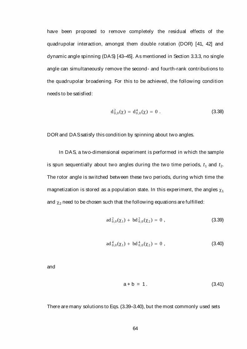
64
have been proposed to remove completely the residual effects of the
quadrupolar interaction, amongst them double rotation (DOR) [41, 42] and
dynamic angle spinning (DAS) [43–45]. As mentioned in Section 3.3.3, no single
angle can simultaneously remove the second- and fourth-rank contributions to
the quadrupolar broadening. For this to be achieved, the following condition
needs to be satisfied:
d 0,02 () d 0 ,0
4 () 0 . (3.38)
DOR and DAS satisfy this condition by spinning about two angles.
In DAS, a two-dimensional experiment is performed in which the sample
is spun sequentially about two angles during the two time periods, t1 and t2.
The rotor angle is switched between these two periods, during which time the
magnetization is stored as a population state. In this experiment, the angles 1
and 2 need to be chosen such that the following equations are fulfilled:
ad 0,02 (1) bd 0,0
2 (2 ) 0 , (3.39)
ad 0,04 (1) bd 0,0
4 (2 ) 0 , (3.40)
and
a + b = 1 . (3.41)
There are many solutions to Eqs. (3.39–3.40), but the most commonly used sets
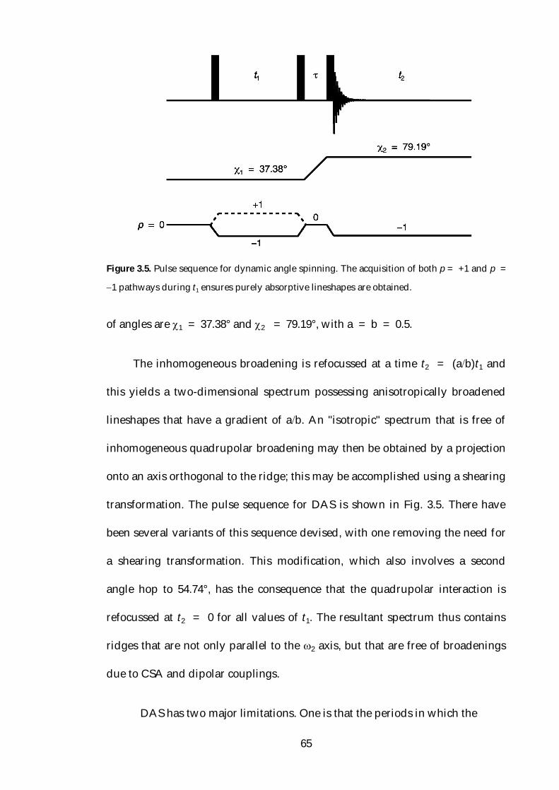
65
Figure 3.5. Pulse sequence for dynamic angle spinning. The acquisition of both p = +1 and p =
1 pathways during t1 ensures purely absorptive lineshapes are obtained.
of angles are 1 = 37.38° and 2 = 79.19°, with a = b = 0.5.
The inhomogeneous broadening is refocussed at a time t2 = (ab)t1 and
this yields a two-dimensional spectrum possessing anisotropically broadened
lineshapes that have a gradient of ab. An "isotropic" spectrum that is free of
inhomogeneous quadrupolar broadening may then be obtained by a projection
onto an axis orthogonal to the ridge; this may be accomplished using a shearing
transformation. The pulse sequence for DAS is shown in Fig. 3.5. There have
been several variants of this sequence devised, with one removing the need for
a shearing transformation. This modification, which also involves a second
angle hop to 54.74°, has the consequence that the quadrupolar interaction is
refocussed at t2 = 0 for all values of t1. The resultant spectrum thus contains
ridges that are not only parallel to the 2 axis, but that are free of broadenings
due to CSA and dipolar couplings.
DAS has two major limitations. One is that the periods in which the

66
Figure 3.6. The arrangement of rotors that forms the basis of the double rotation experiment. In
this experiment, 1 = 54.74 and 2 = 30.56.
magnetization is stored as a population state require long T1 relaxation times, so
making it unsuitable for the many cases in which the T1 relaxation of a
quadrupolar nucleus is very efficient. This has a particularly large effect when a
second angle hop is required for acquisition under MAS conditions. The other
drawback of DAS is that specialist hardware is required for its implementation,
a fact which has limited the applicability of the technique. Nevertheless, several
examples of its utility in 11B [103] and 17O [104–109] NMR have been reported.
In DOR, refocussing of the quadrupolar interaction is achieved by
spinning simultaneously about two angles. This is usually achieved by spinning
the sample in an inner rotor that is itself inside an outer rotor. The outer rotor is
inclined at the magic angle whilst the inner rotor is inclined at an angle of
30.56° to the outer rotor axis. This is shown in Fig. 3.6.
In contrast to DAS, DOR is a one-dimensional experiment. The technique
has major limitations, however. The most significant one arises from the fact
that the outer rotor can usually only be spun at speeds of 1–2 kHz and so the
resultant spectrum is crowded with spinning sidebands that can greatly hinder
67
interpretation. In addition, DOR requires a specialist probe which, as in the case
of DAS, is prone to mechanical problems. In spite of this, DOR has been
successfully applied in 17O [110–115], 23Na [116–123] and 27Al [124–127] NMR.
3.4.3 Multiple-Quantum MAS
3.4.3.1 Introduction
A method was developed in 1995 that achieves complete refocusing of
the second-order quadrupolar interaction [48, 49], and which, unlike DOR and
DAS, may be performed using conventional MAS hardware. This experiment,
known as MQMAS, operates by taking advantage of the fact that the fourth-
rank coefficients of the second-order quadrupolar interaction perturbing the
central and multiple-quantum (usually mI = +32 32) transitions of a half-
integer quadrupolar nucleus differ by a scaling factor. Consequently, a two-
dimensional experiment correlating single-quantum central-transition
coherences and multiple-quantum (MQ) coherences, performed under MAS
conditions, will lead to complete removal of the effects of the quadrupolar
interaction to second order. This is achieved by an experiment in which MQ
coherences are excited and then allowed to evolve in the t1 period before
subsequent conversion to observable central-transition coherences that evolve
during the t2 period. The resultant two-dimensional spectrum contains, after
shearing, a second-order quadrupolar broadened central-transition powder
lineshape parallel to the 2 axis and an isotropic spectrum devoid of

68
quadrupolar broadening parallel to the 1 axis (although fourth-rank
broadenings that are not quadrupolar in origin remain in 1) [128, 129].
3.4.3.2 Non Pure-phase Methods
The original MQMAS experiment involved excitation of either p = 3 or
p = +3 coherences that evolve during the t1 period before their subsequent
conversion to observable central-transition coherence (p = 1) [49]. The pulse
sequence for this experiment is shown in Fig. 3.7, where the two coherence
transfer pathways that may be selected are indicated. In this experiment, single-
pulse excitation has been shown to be better than the two-pulse method [49,
130, 131] used in solution-state NMR [84].
The time-domain signal acquired by the experiment in Fig. 3.7, when
performed on a spin I = 32 nucleus, neglecting chemical shift effects, and
using the solid coherence transfer pathway, is given by:
s(t1 , t2 ) exp iQ
PAS 20
65
Q0 () 65
d 0 ,04 ()Q4 ( , , )
t1
exp iQ
PAS 20
25
Q0 () 5435
d 0,04 ()Q4 ( , , )
t2
. (3.42)
Equation (3.42) thus shows that the fourth-rank contribution to the second-
order quadrupolar broadening is refocussed with the formation of an echo
when

69
Figure 3.7. Pulse sequence and corresponding coherence transfer pathways for the two-pulse
triple-quantum MAS experiment. The +3 1 and 3 1 pathways correspond to the
antiecho and echo pathways for a spin I = 32 nucleus, respectively.
65
t1 5435
t2
0 , (3.43)
i.e., when t2 = (65)(3554)t1 = (79)t1. The position in t2 at which the echo
forms thus depends on the ratio of the fourth-rank coefficients defined in Eq.
(3.22), this is referred to as the MQMAS ratio, R(I, q), and is defined as:
R(I, q)
C4 (I , q)C4 (I, 1 2)
, (3.44)
where q is the coherence order of the transition evolving during the t1 period
and so takes the value ±32 for a triple-quantum MAS experiment.
When t1 = 0, the quadrupolar interaction is refocussed as a half-echo, i.e.,
its signal decreases from its maximum to zero. As t1 increases, the echo moves
progressively forward in t2 until, at a sufficient value of t1, a whole echo is
70
formed. The 3 1 pathway is, for a spin I = 32 nucleus, referred to as the
echo pathway because the echo formed by the refocussing of the residual
second-order quadrupolar interaction moves forward in t2 as t1 increases.
Conversely, the +3 1 pathway is known as the antiecho pathway, in which
case the echo moves backwards in t2 as t1 increases. For a spin I = 52 nucleus,
the situation is reversed. More generally, if the MQMAS ratio is negative, then
the 3 1 coherence transfer pathway is the echo pathway, whilst if it is
positive, then the +3 1 pathway is the echo pathway. The MQMAS ratios for
triple-quantum MAS experiments of spin I = 32, 52 and 72 nuclei are given in
Appendix F.
Two-dimensional Fourier transformation of the data in Eq. (3.42) yields a
two-dimensional spectrum containing an anisotropically broadened ridge
lineshape inclined at a gradient of 79 with respect to the 2 axis. The spectrum
obtained by Fourier transformation of the signal arising from the +3 1
(antiecho) pathway contains a ridge lineshape inclined at a gradient of 79. In
each case, an isotropic spectrum may then be obtained by projection onto an
axis orthogonal to this ridge, in a manner exactly analogous to DAS that was
described earlier.
Inspection of Eq. (3.42) shows that the signal yielded from these two-pulse
MQMAS methods is phase modulated and hence, the resultant two-
dimensional spectrum contains lineshapes that are not pure-phase (i.e., they
contain the highly undesirable phase-twist). Consequently, these experiments
are not suitable for modern NMR spectroscopy and are no longer routinely

71
used.
3.4.3.3 Pure-phase Methods
It has been observed that for a spin I = 32 nucleus, the 3 1 and +3
1 conversions are equally efficient when a hard pulse with an inherent flip
angle of = 90 is used [132]. By performing a two-dimensional experiment in
which the 3 1 and +3 1 coherence transfer pathways are
simultaneously selected such that p = 3 and p = + 3 coherences evolve
during the t1 period, a spectrum containing absorption-mode lineshapes may be
obtained [132]. There is, however, no pulse flip angle which can perform these
coherence transfer processes with equal efficiency for nuclei with spin I > 32
and consequently, such an experiment has not been widely used.
A modification of the experiment described above that can lead to absorption-
mode two-dimensional lineshapes for all values of I was suggested in 1996. This
experiment also involves simultaneous evolution of p = +3 and p = 3
coherences during the t1 period, but their conversion to observable central-
transition coherences is achieved using two pulses that proceed via a
population state (p = 0). This method, known as a z-filter [133–135], achieves
the acquisition of purely absorption-mode lineshapes by utilising the fact that
the +3 0 and 3 0 conversions are always equally efficient. The pulse
sequence and coherence transfer pathway is shown in Fig. 3.8a, where the last
pulse is a 90 pulse selective for the central transition. The acquisition of both p
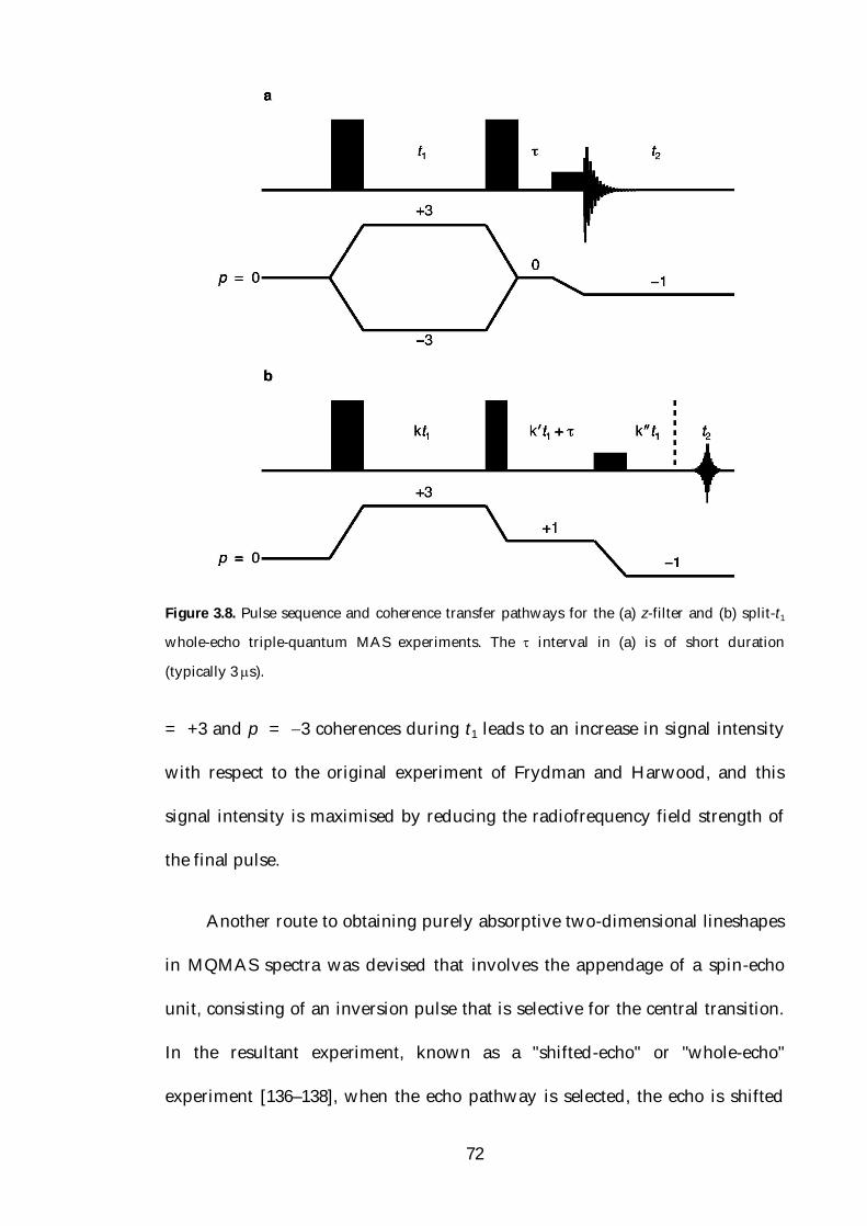
72
Figure 3.8. Pulse sequence and coherence transfer pathways for the (a) z-filter and (b) split-t1
whole-echo triple-quantum MAS experiments. The interval in (a) is of short duration
(typically 3 s).
= +3 and p = 3 coherences during t1 leads to an increase in signal intensity
with respect to the original experiment of Frydman and Harwood, and this
signal intensity is maximised by reducing the radiofrequency field strength of
the final pulse.
Another route to obtaining purely absorptive two-dimensional lineshapes
in MQMAS spectra was devised that involves the appendage of a spin-echo
unit, consisting of an inversion pulse that is selective for the central transition.
In the resultant experiment, known as a "shifted-echo" or "whole-echo"
experiment [136–138], when the echo pathway is selected, the echo is shifted

73
forward in t2 by a time , where is the echo interval. This means that,
assuming a sufficiently long value of is chosen, the residual second-order
quadrupolar interaction is refocussed as a whole echo for every value of t1. In
addition, the echo is no longer formed at t2 < 0 for the antiecho pathway.
The fact that a choice of echo interval can be made such that the
quadrupolar interaction is refocussed as a whole echo for all values of t1 means
that this experiment yields a spectrum containing purely absorptive two-
dimensional lineshapes. This occurs as a result of the properties of whole
echoes. Whole echoes contain real and imaginary components that are
symmetric and anti-symmetric about the midpoint, respectively. The Fourier
transform of such a time-domain signal yields a lineshape in which the real part
is purely absorptive and the imaginary part is zero. It is for this reason that such
a modification to the experiment has become routine as a way of obtaining
pure-phase two-dimensional lineshapes in MQMAS. It should be noted that the
symmetry properties of a whole echo only hold in cases where the
inhomogeneous broadening exceeds the homogeneous broadening [136]. This is
typically the case for crystalline materials but in amorphous or disordered
materials this is often not observed and, in such cases, whole-echo methods are
not the optimum choice.
It was shown in Section 3.4.3.2 that the residual fourth-rank quadrupolar
broadening is refocussed, when the echo pathway is selected, when t2 = (C4(I,
32)C4(I, 12))t1, so leading to a spectrum with an anisotropically broadened
ridge aligned along a gradient equal to the MQMAS ratio. To obtain an
74
isotropic spectrum it is necessary to perform a shearing transformation; this
produces a spectrum in which the ridge is parallel to the 2 axis and an
isotropic spectrum is then obtained directly from a projection onto the 1 axis
[139]. However, a further modification to the MQMAS experiment has been
devised which directly produces a spectrum in which the quadrupolar
broadened ridge is parallel to the 2 axis, so avoiding the need for a shearing
transformation. This is achieved by performing a shifted-echo experiment in
which the t1 period is split into periods of multiple-quantum and central-
transition evolution [134, 137, 138]. In such an experiment, the inhomogeneous
broadening is refocussed at the end of the t1 period and a whole echo formed at
t2 = for all values of t1. To illustrate this, consider the example of a spin I =
32 nucleus. The MQMAS ratio in this case has the value 79; that is, the fourth-
rank contribution to the inhomogeneous broadening from the triple-quantum
transition is 79 of that arising from the central transition. Consequently, if the
t1 period is split into periods of triple-quantum and central-transition evolution
in the ratio 9:7, the fourth-rank contribution to the second-order quadrupolar
interaction will be refocussed at the end of t1 for all values of t1.
The division of the t1 period into periods of triple-quantum and central-
transition evolution is the basis of so-called "split-t1" acquisition in MQMAS
experiments. The pulse sequence for these experiments is shown in Fig. 3.8b.
Split-t1 acquisition is usually combined with the shifted-echo method so as to
produce an experiment that yields both ridge lineshapes parallel to the F2 axis
and pure-phase two-dimensional lineshapes. The experiment shown in Fig. 3.8b

75
is thus referred to as a split-t1 whole-echo MQMAS experiment and is
applicable to all the multiple-quantum transitions of every half-integer
quadrupolar nucleus. The values of the constants k, k’ and k’’ in Fig. 3.8b are
given, for spin I = 32, 52 and 72 nuclei, in Appendix G. For nuclei possessing
triple-quantum transitions with a positive MQMAS ratio, the period of central-
transition evolution during t1 has p = 1 (i.e., k’ = 0), as in such cases, a
correlation between triple-quantum and single-quantum transitions of opposite
sign is required for refocussing of the fourth-rank inhomogeneous broadening
to occur at t2 > 0.
The MQMAS experiment is now a routine method for obtaining high-
resolution NMR spectra of quadrupolar nuclei and there have been numerous
examples demonstrating its applicability to nuclei with a range of spin
quantum numbers, such as 11B [140–145], 17O [146–161], 23Na [162–173], 25Mg
[174, 175], 27Al [176–194], 43Ca [195–198], 45Sc [199, 200], 51V [201, 202], 55Mn
[203], 59Co [204, 205], 63Cu [206], 87Rb [136, 207, 208] and 93Nb [209–214].
3.4.4 Satellite-Transition MAS
Another method that facilitates the acquisition of isotropic spectra of
quadrupolar nuclei is the STMAS experiment, introduced in 2000 [50]. This
experiment operates in an analogous manner to MQMAS, but instead uses a
correlation of satellite-transition coherences with central-transition coherences
to achieve refocussing of the residual fourth-rank quadrupolar broadening. The

76
Figure 3.9. Pulse sequence and coherence transfer pathway for the phase-modulated whole-
echo STMAS experiment. Split-t1 acquisition is used and the constants k, k’ and k” are given in
Appendix G.
acquisition of whole echoes is typically used to ensure the acquisition of
absorption-mode two-dimensional lineshapes. The resultant two-dimensional
spectrum, if obtained using split-t1 acquisition, consists of an ST
CTcorrelation ridge for each inequivalent site in the solid, each of which is
broadened by the residual second-order quadrupolar interaction parallel to the
2 axis and that is free from quadrupolar broadening parallel to the 1 axis.
In Section 3.3.3 it was shown that rotor-synchronized MAS removes the
effects of any second-rank interaction, such as the first-order quadrupolar
interaction. Consequently, as the satellite transitions in a quadrupolar nucleus
are subject to a large first-order quadrupolar perturbation, very accurate rotor-
synchronization is required during the t1 period. To fully remove the effects of
the first-order quadrupolar interaction, the magic angle must also be set very
precisely (within 0.003) [53].
STMAS spectra are typically acquired using the phase-modulated split-t1
whole-echo pulse sequence in Fig. 3.9. This experiment yields a two-
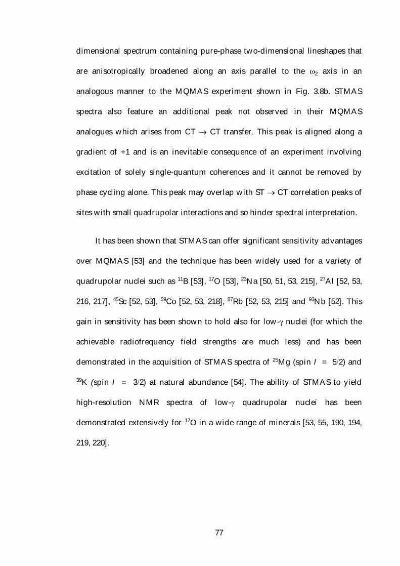
77
dimensional spectrum containing pure-phase two-dimensional lineshapes that
are anisotropically broadened along an axis parallel to the 2 axis in an
analogous manner to the MQMAS experiment shown in Fig. 3.8b. STMAS
spectra also feature an additional peak not observed in their MQMAS
analogues which arises from CT CT transfer. This peak is aligned along a
gradient of +1 and is an inevitable consequence of an experiment involving
excitation of solely single-quantum coherences and it cannot be removed by
phase cycling alone. This peak may overlap with ST CT correlation peaks of
sites with small quadrupolar interactions and so hinder spectral interpretation.
It has been shown that STMAS can offer significant sensitivity advantages
over MQMAS [53] and the technique has been widely used for a variety of
quadrupolar nuclei such as 11B [53], 17O [53], 23Na [50, 51, 53, 215], 27Al [52, 53,
216, 217], 45Sc [52, 53], 59Co [52, 53, 218], 87Rb [52, 53, 215] and 93Nb [52]. This
gain in sensitivity has been shown to hold also for low- nuclei (for which the
achievable radiofrequency field strengths are much less) and has been
demonstrated in the acquisition of STMAS spectra of 25Mg (spin I = 52) and
39K (spin I = 32) at natural abundance [54]. The ability of STMAS to yield
high-resolution NMR spectra of low- quadrupolar nuclei has been
demonstrated extensively for 17O in a wide range of minerals [53, 55, 190, 194,
219, 220].
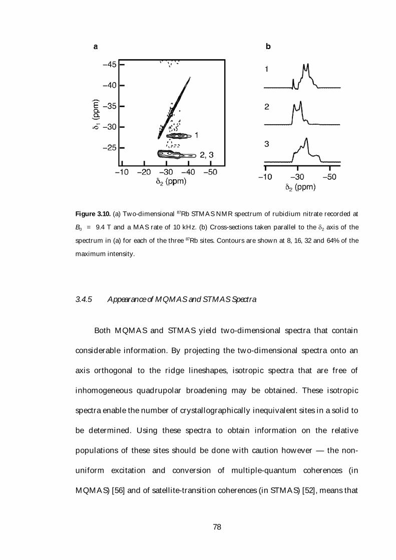
78
Figure 3.10. (a) Two-dimensional 87Rb STMAS NMR spectrum of rubidium nitrate recorded at
B0 = 9.4 T and a MAS rate of 10 kHz. (b) Cross-sections taken parallel to the 2 axis of the
spectrum in (a) for each of the three 87Rb sites. Contours are shown at 8, 16, 32 and 64% of the
maximum intensity.
3.4.5 Appearance of MQMAS and STMAS Spectra
Both MQMAS and STMAS yield two-dimensional spectra that contain
considerable information. By projecting the two-dimensional spectra onto an
axis orthogonal to the ridge lineshapes, isotropic spectra that are free of
inhomogeneous quadrupolar broadening may be obtained. These isotropic
spectra enable the number of crystallographically inequivalent sites in a solid to
be determined. Using these spectra to obtain information on the relative
populations of these sites should be done with caution however — the non-
uniform excitation and conversion of multiple-quantum coherences (in
MQMAS) [56] and of satellite-transition coherences (in STMAS) [52], means that

79
these techniques are not quantitative. This is discussed in greater detail in
Chapter 4. A typical spectrum of a crystalline material obtained using these
methods is presented in Fig. 3.10, where the 87Rb STMAS NMR spectrum of
rubidium nitrate, RbNO3, is shown. The two-dimensional spectrum in Fig. 3.10a
shows the expected ST CT ridges for each of the three sites [221] present,
along with the superfluous CT CT correlation ridge. Cross-sections taken
parallel to the 2 axis for each of the three sites yield second-order quadrupolar
broadened lineshapes whose width, shape and position in the two-dimensional
spectrum are dependent on the values of CQ and of each of the sites in this
material [136].
MQMAS and STMAS have the great advantage over one-dimensional
high-resolution methods such as DOR that the resultant spectra possess two
dimensions in which quadrupolar information is retained [136]. Quadrupolar
parameters may be extracted from MQMAS and STMAS spectra by analysis of
the position of the centre of gravity of each ridge lineshape in the 1 and 2
dimensions. These positions depend on the isotropic chemical shift, CS, and Q,
the isotropic second-order quadrupolar shift, which is given by
Q
QPAS 20
1 2
3
, (3.45)
expressed as a ppm shift. It can be shown that for a spin I = 32 nucleus the
peak positions in the 1 and 2 dimensions of a sheared or split-t1 triple-
quantum MAS spectrum are given by:

80
1
178
CS 12Q , (3.46)
and
2 CS
25Q , (3.47)
and by rearranging:
CS
81 102
27 , (3.48)
and
Q
2161 4592
160 . (3.49)
The expressions in Eqs. (3.46) and (3.47) are different for spectra obtained
by non-split-t1 methods or for those that have not been subject to a shearing
transformation and these are shown, for both MQMAS and STMAS
experiments of spin I = 32 and I = 52 nuclei, in Appendix H. If the peak
positions in the two dimensions are known, then the quadrupolar parameters
CS and Q may be determined. It is not possible to obtain CQ and
independently from Q, however, the quadrupolar product PQ, defined as [107]:
PQ CQ 1
2
3
, (3.50)
81
may be determined from Q by
PQ
2I(2I 1)0 Q
3 103 . (3.51)
3.4.5.1 Spectra of Amorphous Materials
In unsheared MQMAS and STMAS spectra, or spectra acquired from non-
split-t1 methods, the anisotropically broadened ridge lineshapes lie along an
axis given by the MQMAS or STMAS ratio, typically known as the anisotropic
(A) axis. In amorphous and disordered materials, the lineshapes may be
broadened along additional axes due to a distribution of isotropic chemical
shifts and second-order quadrupolar shifts [222]. Where there is a distribution
of isotropic chemical shifts, the ridges are broadened along an axis that has a
gradient of +1 in the case of STMAS and +3 for triple-quantum MAS. This axis
is usually referred to as the chemical shift (CS) axis. If there is also a range of
second-order quadrupolar broadenings, then the lineshape will also be
broadened along an axis with a gradient given by the ratio
2/1,A
),(A0
0
IqI
, (3.52)
where A0(I, q) and A0(I, 12) are the spin- and transition-dependent zeroth-rank
coefficients introduced in Section 3.3.2. This axis is known as the quadrupolar
shift (QS) axis.

82
The ability of MQMAS and STMAS to identify distributions of isotropic
chemical shifts and isotropic second-order quadrupolar shifts demonstrates the
great utility of these techniques when considering the structure of amorphous
materials.

83
Chapter 4
Coherence Transfer Enhancement
4.1 Selective and Non-Selective Pulses
An important parameter in NMR is the inherent nutation frequency, 1,
related to the radiofrequency field strength, B1, by 1 = B1. When an NMR
experiment is performed, it is desirable to have a nutation frequency much
greater than the range of resonance frequencies being studied. Under such
conditions the effective field, Beff, experienced by all the spins whose
frequencies are in the range being studied, is virtually constant. Using the
vector model description of NMR described in Section 2.2, this means that the
magnetization vectors of all the spins are rotated through the same flip angle by
the pulse. A pulse that has this effect is known as a "hard" or non-selective
pulse. In the context of quadrupolar nuclei, a hard pulse is one for which the
following condition is satisfied:
1 >> Q . (4.1)
For half-integer quadrupolar nuclei in the solid state, however, this is rarely the
case. In a powdered sample, Q takes values ranging from zero to QPAS .
Consequently, Eq. (4.1) is not satisfied for the majority of the crystallites, even
with the highest radiofrequency field strengths currently attainable (typically
84
300 kHz), and so the following condition now applies:
1 << Q , (4.2)
in which case the pulse is referred to as "soft" or selective and only the central
transition is excited. For the majority of crystallites, the ratio Q1 is thus much
greater than unity. In this section, the effect of the range of values of Q1 on
single-pulse single-quantum coherence excitation is shown, whilst in the
subsequent sections the coherence transfer processes present in MQMAS is
considered.
To consider the effect of pulses in the hard and soft regimes, the evolution
of the density operator needs to be determined. The Liouville-von Neumann
equation, introduced in Chapter 2, describes the evolution of the density
operator. For a hard pulse along the rotating frame x axis, the Hamiltonian is
given by 1Ix, and so for an initial density operator at thermal equilibrium this
equation takes the form
d(t )d t
i 1Ix , Iz
1Iy
. (4.3)
This equation describes the nutation of the magnetization from the z axis to the
y axis at a rate 1.
When a soft pulse is applied to a half-integer quadrupolar nucleus, only
the central transition is excited. In such a situation, only two energy levels need
85
to be considered (those with mI = +12 and mI = 12) and so half-integer
quadrupolar nuclei may be treated like spin I = 12 nuclei. In such cases, a
convenient method for determining the effect of a soft pulse is the fictitious
spin-12 operator formalism [223–226], which was introduced in 1977 for a spin
I = 1 nucleus [224]. In this formalism, the matrix representations of the
operators Ix(1 / 2,1 / 2) and Iy
(1 / 2 ,1 / 2) are given by, for a spin I = 32 nucleus:
Ix(1 / 2,1 / 2)
12
0 0 0 00 0 1 00 1 0 00 0 0 0
Iy(1 / 2,1 / 2)
12
0 0 0 00 0 i 00 i 0 00 0 0 0
. (4.4)
The central 2 2 elements of these matrices are of course identical to the matrix
representations of the angular momentum operators for a spin I = 12 nucleus
given in Appendix A. Using these operators, the evolution of the density
operator can be shown to be, for a nucleus with spin quantum number I:
d(t )d t
i I 12
1Ix
(1 / 2 ,1 / 2 ) , Iz
I 12
1Iy
(1/ 2 ,1 / 2)
. (4.5)
A comparison of Eqs. (4.3) and (4.5) reveals that the nutation frequency is (I +

86
Figure 4.1. The dependence of signal intensity on the flip angle of an on-resonance excitation
pulse for a spin I = 32 nucleus, shown for when Q1 is equal to 0 (solid line), 1 (dotted line)
and 25 (dashed line). Simulations were performed assuming the sample to be static and
assuming the presence of a second-order quadrupolar interaction with = 0. The simulations
were performed by assuming 90 equally-spaced values of the angle . The vertical scale is
normalised with respect to the maximum single-quantum coherence obtained with a soft pulse.
12) times greater for a selective pulse compared to a non-selective one.
This variation in nutation frequency is demonstrated in Fig. 4.1 for a spin I
= 32 nucleus, where the dependence of the central-transition signal intensity is
shown as a function of the excitation pulse flip angle for ratios of Q1 equal to
0, 1 and 25. The increase in nutation frequency for a soft pulse means that it
leads to a maximum in signal intensity at a flip angle (for a spin I = 32
nucleus) of 45, half the 90 observed in the hard pulse case. In addition, this
also means that there is a null in signal intensity observed for a soft pulse at a
flip angle of 90, half the 180 observed for a hard pulse. The increase in
nutation frequency shown in Fig. 4.1 also leads to an (I + 12) factor reduction in
the signal intensity obtained when a pulse selective for the central transition is

87
used compared with a hard pulse.
4.2 Excitation of Multiple-Quantum Coherence
The excitation of multiple-quantum coherence [227, 228] plays an
important role in a wide range of NMR experiments. Even though only single-
quantum coherence may be directly detected in NMR, excitation of multiple-
quantum coherence of spin I = 12 nuclei in liquids is found in a variety of
experiments such as DQF-COSY [229, 230], HMQC [231] and INADEQUATE
[232]. The use of double- and triple-quantum filtration methods as a means of
measuring the relaxation rates of spin I = 32 nuclei in liquids and of
differentiating between nuclear environments has also been shown [233, 234].
In the solid state, it was shown in 1981 that triple-quantum coherence may be
excited for spin I = 32 nuclei [235].
When working in the liquid state, multiple-quantum excitation is typically
achieved via a two-pulse method [84]. Likewise, in the original MQMAS
experiment, two-pulse excitation was used [48, 49]. It has been shown,
however, that a single-pulse excitation is more efficient when 1 < QPAS [225]
and excitation of triple-quantum coherence for spin I 32 nuclei has been
shown [236, 237] and implemented into triple-quantum MAS [207] successfully
using this method. Using the single-transition operator formalism, Wokaun and
Ernst have shown that triple-quantum excitation in spin I = 32 nuclei yields a
signal that may be quantified in terms of the expectation value of the operator

88
Iy(3 / 2 ,3 / 2 ) [225]:
tty 2Q
31)2/3,2/3(
83
sin23)(I , (4.6)
and consequently, the duration of a triple-quantum excitation pulse that yields
the optimum amplitude of triple-quantum coherence, exmax , is given by
ex
max 83
Q
1
2
90max , (4.7)
where the optimum signal amplitude obtained by a 90 pulse has a duration,
90max , given by:
90
max
21 . (4.8)
It can also be shown that the excitation of single-quantum coherence reaches its
maximum value when the duration of the pulse, p 1max , is
p 1
max 90
max
2 45o . (4.9)
This is consistent with Section 4.1, in which it was shown that the nutation
frequency of the central transition is (I + 12) times faster in the limit 1 < Q.
The dependence of triple-quantum excitation on the pulse flip angle is
shown as a function of the ratio Q1 in Fig. 4.2, where the amplitude of triple-

89
Figure 4.2. Dependence of the triple-quantum signal intensity on the flip angle of the excitation
pulse, shown for a spin I = 32 nucleus for Q1 equal to 2 (solid line), 4 (dotted line) and 8
(dashed line). The y axis scale is normalised as in Fig. 4.1 and all other simulation parameters
are the same as those used in Fig. 4.1.
quantum coherence excited is defined as the magnitude of the tensor operator
T3,3 (p = 3 coherence) obtained when single-pulse excitation is performed on
the operator T1,0. When Q1 is 2, triple-quantum excitation reaches its
optimum at a flip angle of 218, whilst flip angles of 267 and 251 yield
maximum triple-quantum signal intensity when this ratio is equal to 4 and 8,
respectively. The triple-quantum amplitudes are comparable to the central
transition amplitudes obtained in Fig 4.1, so indicating that triple-quantum
excitation is a relatively efficient process.
The three curves in Fig. 4.2 show that a factor of four increase in the ratio
Q1 leads to an approximate 60% reduction in the triple-quantum signal
intensity. Given that in a powder the quadrupolar coupling parameter Q can
take values ranging from zero to QPAS , this means that each crystallite in a
powder does not lead to equal triple-quantum excitation.

90
The observations made using Fig. 4.2 have been considered in greater
detail in the literature [56, 237], where the triple-quantum excitation behaviour
of half-integer quadrupolar nuclei has been demonstrated [56]. In addition, the
effect of MAS has also been considered [238].
4.3 Conversion of Multiple-Quantum Coherence
The original MQMAS experiment [48, 49] consisted of two steps — the
excitation of triple-quantum coherence and its conversion to observable central-
transition coherence. The signal intensity obtained from this experiment when
either the 3 1 or +3 1 coherence transfer pathway is selected is shown
in Figs. 4.3a and 4.3b respectively, as a function of the flip angle of the
conversion pulse when the ratio Q1 is equal to 2, 4 and 8. Figure 4.3a shows
that when the 3 1 pathway is selected, the maximum signal intensity is
obtained when the conversion pulse has a flip angle close to 60. When the +3
1 pathway is selected, Fig. 4.3b reveals maximum signal intensity to occur
at a flip angle of approximately 95. In both cases the reduction in signal
intensity as the quadrupolar coupling parameter is increased, which was also
observed for triple-quantum excitation in Fig. 4.2, is seen.
One obvious feature evident in both Figs. 4.3a and 4.3b is that the signal
intensity is greatly reduced with respect to Fig. 4.2. This indicates that the
conversion of triple-quantum coherences is a far less efficient process than
triple-quantum excitation. Closer inspection reveals that, for a spin I = 32

91
a
b
Figure 4.3. Dependence of the signal intensity obtained for a spin I = 32 nucleus in the (a) 3
1 and (b) +3 1 MQMAS experiments as a function of the flip angle of the conversion
pulse, with the ratio Q1 equal to 2 (solid line), 4 (dotted line) and 8 (dashed line). The flip
angle of the triple-quantum excitation pulse is 240; all other parameters are as in Fig. 4.2.
nucleus, the conversion of triple-quantum coherences via the 3 1 and +3
1 pathways is equally efficient when a pulse with a flip angle of 90 is used.
This has the implication that, by performing an amplitude-modulated MQMAS

92
Figure 4.4. Dependence of the signal intensity on the quadrupolar coupling parameter, CQ,
using the two-pulse MQMAS experiment in Fig. 3.7 (selecting the 3 1 pathway). The signal
intensity is shown for the cases where the radiofrequency field strength is equal to 100 kHz
(solid line), 200 kHz (dotted line) and 300 kHz (dashed line). The flip angles of the excitation
and conversion pulses are 240 and 60, respectively; all other parameters are as in Fig. 4.2.
experiment in which both p = +3 and p = 3 coherences are selected during
the t1 period (described earlier in Section 3.4.3.3), a two-dimensional spectrum
may be obtained that contains pure- phase lineshapes [207]. Such behaviour is,
however, only observed for spin I = 32 nuclei and hence such an experiment
has not found widespread application.
The dependence of the signal intensity obtained from the MQMAS
experiment used in Fig. 4.3a on the quadrupolar coupling is demonstrated in
Fig. 4.4, where the signal intensity is shown as a function of the quadrupolar
coupling parameter, CQ. Figure 4.4 shows how the maximum signal intensity
obtained occurs at a higher value of the quadrupolar coupling constant as the
hard-pulse field strength is increased; this is consistent with Eq. (4.6). It is seen
that, for a radiofrequency field strength 12 = 100 kHz, the experiment is at

93
its most efficient when CQ is ~0.6 MHz. Clearly, for significant signal intensity
to be obtained for nuclei with CQ greater than 2 MHz a much higher B1 field is
required. The highest B1 field currently achievable with commercial MAS
probes is ~300 kHz and as shown in Fig. 4.4, the maximum efficiency of the
MQMAS experiment occurs when CQ ~1.7 MHz in this case. Clearly, MQMAS
performs poorly in the presence of large quadrupolar interactions. It is also
evident from Fig. 4.4 that a single pulse will fail to excite multiple-quantum
coherences if the field strength is too large [225].
Figure 4.4 demonstrates what is arguably the greatest limitation of the
MQMAS experiment, specifically the lack of sensitivity for nuclei with large
quadrupolar interactions. This has the consequence that the intensities of
resonances arising from crystallographically inequivalent sites do not
accurately reflect the site populations predicted from the crystal structure.
The non-uniform excitation and conversion of triple-quantum coherences
also has the effect that it can lead to distortions in the quadrupolar lineshapes.
The range of values of the quadrupolar coupling parameter Q observed in a
powder means that the multiple-quantum filtered spectrum of a static sample
exhibits significant distortions. In particular, crystallites with Q = 0 do not
yield any signal due to the failure to excite multiple-quantum coherence in the
absence of a quadrupolar interaction. Under MAS conditions distortions are
typically minimal as a result of the time dependence imposed on the
quadrupolar interaction under spinning conditions, although they can be
significant when the ratio Q1 is large.
94
Figure 4.3 demonstrates the inefficiency of the conversion step in the
MQMAS experiment. In STMAS, the conversion of satellite-transition to
central-transition coherences is also an inefficient process [53, 54] and so, like
MQMAS, the experiment can suffer from poor sensitivity in the presence of
large quadrupolar interactions. In addition, the excitation and conversion of
satellite-transition coherences is dependent on the magnitude of the
quadrupolar interaction and so, like MQMAS, STMAS is a non-quantitative
technique.
4.4 Methods for Enhanced Coherence Transfer
It was shown in the previous section that the inefficiency of the excitation
and conversion processes is one of the major weaknesses of the MQMAS (and
STMAS) experiments. The first efforts to remedy this situation focussed on
improving the efficiency of the excitation of triple-quantum coherences in
MQMAS. The use of composite pulses has been shown to yield a 30% increase
in signal intensity with respect to single-pulse excitation [239], whilst shaped
pulses have also been shown to provide useful enhancements [240]. More
recent efforts have predominantly focussed on addressing the inefficiency of
the conversion step in MQMAS. This has led to the development of several
methods that increase the signal intensity obtained from MQMAS, such as fast
amplitude-modulated (FAM) pulses [57, 241–243], hyperbolic secant pulses
(HS) pulses [244], double frequency sweeps (DFS) [245, 246], rotationally-
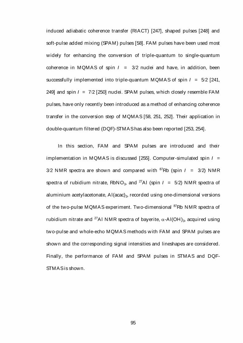
95
induced adiabatic coherence transfer (RIACT) [247], shaped pulses [248] and
soft-pulse added mixing (SPAM) pulses [58]. FAM pulses have been used most
widely for enhancing the conversion of triple-quantum to single-quantum
coherence in MQMAS of spin I = 32 nuclei and have, in addition, been
successfully implemented into triple-quantum MQMAS of spin I = 52 [241,
249] and spin I = 72 [250] nuclei. SPAM pulses, which closely resemble FAM
pulses, have only recently been introduced as a method of enhancing coherence
transfer in the conversion step of MQMAS [58, 251, 252]. Their application in
double-quantum filtered (DQF)-STMAS has also been reported [253, 254].
In this section, FAM and SPAM pulses are introduced and their
implementation in MQMAS is discussed [255]. Computer-simulated spin I =
32 NMR spectra are shown and compared with 87Rb (spin I = 32) NMR
spectra of rubidium nitrate, RbNO3, and 27Al (spin I = 52) NMR spectra of
aluminium acetylacetonate, Al(acac)3, recorded using one-dimensional versions
of the two-pulse MQMAS experiment. Two-dimensional 87Rb NMR spectra of
rubidium nitrate and 27Al NMR spectra of bayerite, -Al(OH)3, acquired using
two-pulse and whole-echo MQMAS methods with FAM and SPAM pulses are
shown and the corresponding signal intensities and lineshapes are considered.
Finally, the performance of FAM and SPAM pulses in STMAS and DQF-
STMAS is shown.

96
4.4.1 FAM and SPAM Pulses
FAM pulses commonly come in two forms. FAM-I pulses involve a train
of alternate phase hard pulses interleaved with delays; the pulses and delays
being of equal duration [57, 241]. FAM-II pulses involve two alternate phase
hard pulses of unequal duration, applied in succession [242]. These pulses may
be used in enhancing the triple-quantum to single-quantum coherence
conversion process if a change in coherence order p = 2 (i.e., ±3 ±1) is
required, although it has been reported that FAM-I pulses are more effective in
enhancing coherence transfer where p = 4 and that FAM-II pulses perform
better when p = 2 [241]. Only FAM-II pulses are considered in the
experimental results shown in this chapter and so these will be referred to
henceforth simply as FAM pulses.
SPAM pulses are, like FAM pulses, composite pulses [256], consisting of a
hard pulse followed immediately by a soft pulse that acts as a selective 90
pulse on the central transition. The signal intensity yielded by SPAM pulses is
at its maximum when the hard pulse duration is optimised to yield maximum
3 0 transfer [58, 251], and so is identical to the optimum value found in a z-
filter experiment [135]. The relative phase of the two components of a SPAM
pulse depends on whether the multiple-quantum coherence to central-
transition coherence conversion step involves a change in sign of coherence
order [58, 251].
The implementation of FAM and SPAM pulses in MQMAS is shown in

97
Figure 4.5. (a) Two-pulse sequence for the (triple-quantum) MQMAS experiment. (b) Phase-
modulated version of the whole-echo (triple-quantum) MQMAS experiment. The shaded
conversion pulse in (a) and (b) can either be a single hard pulse, a composite FAM pulse, or a
composite SPAM pulse, as shown in (c). The two components of the SPAM pulse have the same
phase for ±3 1 transfer and the opposite phase for ±3 ±1 transfer.
Fig. 4.5. As seen in Fig. 4.5a, FAM and SPAM pulses may easily be inserted into
the conversion step of the two-pulse MQMAS experiment. They are also ideally
suited to insertion into the +3 +1 conversion step of phase-modulated split-t1

98
Figure 4.6. Dependence of the central-transition amplitude on the flip angle of the conversion
pulse in the 3 1 MQMAS experiment for a spin I = 32 nucleus. Plots are shown for when
a single hard pulse is used (solid line) and for the first and second hard pulses in a FAM pulse
(dotted and dashed lines, respectively). When the first FAM pulse is incremented, the second
pulse has a flip angle of 43, whilst a flip angle of 88 is used for the first pulse when the second
one is being varied. The y axis scale is normalised with respect to the signal intensity obtained
when an optimised single hard pulse is used. Simulations were performed assuming a
radiofrequency field strength of 100 kHz, a quadrupolar coupling constant of 2.0 MHz and a
Larmor frequency of 100 MHz. The excitation pulse flip angle is 240. All other parameters are
as in Fig. 4.2.
whole-echo methods, as shown in Fig. 4.5b. Aside from providing signal
enhancement, it has been reported that SPAM pulses, when used in the echo
and antiecho versions of the two-pulse MQMAS experiment, yield very similar
signal intensities [58, 251]. This has led to the suggestion that combining data
obtained from the SPAM-echo and SPAM-antiecho experiments is an effective
method for recording high-resolution MQMAS spectra with enhanced
sensitivity [251].
Figure 4.6 shows the dependence of the signal intensity obtained, for a
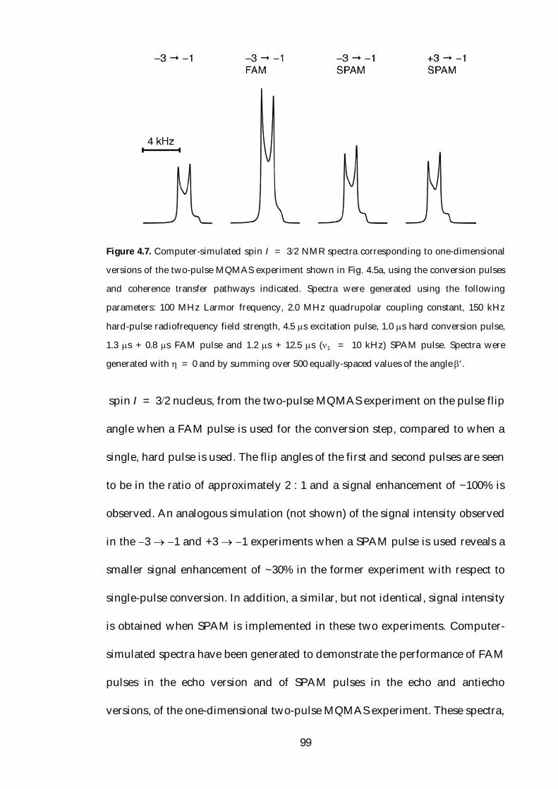
99
Figure 4.7. Computer-simulated spin I = 32 NMR spectra corresponding to one-dimensional
versions of the two-pulse MQMAS experiment shown in Fig. 4.5a, using the conversion pulses
and coherence transfer pathways indicated. Spectra were generated using the following
parameters: 100 MHz Larmor frequency, 2.0 MHz quadrupolar coupling constant, 150 kHz
hard-pulse radiofrequency field strength, 4.5 s excitation pulse, 1.0 s hard conversion pulse,
1.3 s + 0.8 s FAM pulse and 1.2 s + 12.5 s (1 = 10 kHz) SPAM pulse. Spectra were
generated with = 0 and by summing over 500 equally-spaced values of the angle .
spin I = 32 nucleus, from the two-pulse MQMAS experiment on the pulse flip
angle when a FAM pulse is used for the conversion step, compared to when a
single, hard pulse is used. The flip angles of the first and second pulses are seen
to be in the ratio of approximately 2 : 1 and a signal enhancement of ~100% is
observed. An analogous simulation (not shown) of the signal intensity observed
in the 3 1 and +3 1 experiments when a SPAM pulse is used reveals a
smaller signal enhancement of ~30% in the former experiment with respect to
single-pulse conversion. In addition, a similar, but not identical, signal intensity
is obtained when SPAM is implemented in these two experiments. Computer-
simulated spectra have been generated to demonstrate the performance of FAM
pulses in the echo version and of SPAM pulses in the echo and antiecho
versions, of the one-dimensional two-pulse MQMAS experiment. These spectra,
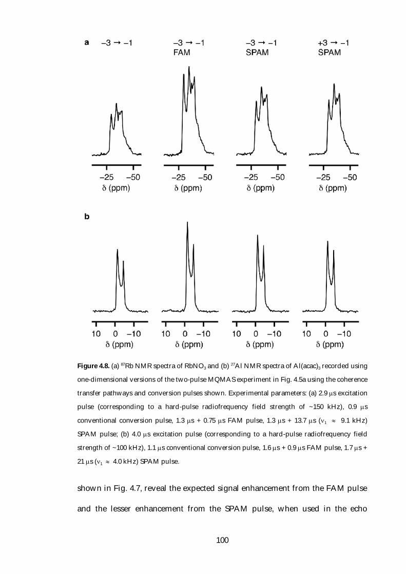
100
Figure 4.8. (a) 87Rb NMR spectra of RbNO3 and (b) 27Al NMR spectra of Al(acac)3 recorded using
one-dimensional versions of the two-pulse MQMAS experiment in Fig. 4.5a using the coherence
transfer pathways and conversion pulses shown. Experimental parameters: (a) 2.9 s excitation
pulse (corresponding to a hard-pulse radiofrequency field strength of ~150 kHz), 0.9 s
conventional conversion pulse, 1.3 s + 0.75 s FAM pulse, 1.3 s + 13.7 s (1 9.1 kHz)
SPAM pulse; (b) 4.0 s excitation pulse (corresponding to a hard-pulse radiofrequency field
strength of ~100 kHz), 1.1 s conventional conversion pulse, 1.6 s + 0.9 s FAM pulse, 1.7 s +
21 s (1 4.0 kHz) SPAM pulse.
shown in Fig. 4.7, reveal the expected signal enhancement from the FAM pulse
and the lesser enhancement from the SPAM pulse, when used in the echo
101
version of the experiment. When implemented into the antiecho version, the
SPAM pulse yields slightly less signal intensity than that obtained from the
echo experiment. In the case of both FAM and SPAM pulses, minimal lineshape
distortions are observed.
The performance of FAM and SPAM pulses in enhancing coherence
transfer in MQMAS has been considered using two crystalline materials. Figure
4.8 shows one-dimensional MQMAS spectra of rubidium nitrate and
aluminium acetylacetonate recorded using the conversion pulses and coherence
transfer pathways indicated.
For both spin I = 32 and spin I = 52 nuclei, FAM pulses are shown to
yield the most signal intensity. SPAM pulses result in a smaller, but still very
useful, enhancement with respect to a single hard pulse, whilst the two versions
of the SPAM pulse yield very similar, but not identical signal intensities for the
echo and antiecho pathways. These observations confirm the validity of the
spin I = 32 computer-simulated spectra in Fig. 4.7.
4.4.2 Two-Dimensional MQMAS NMR
The application of FAM and SPAM pulses to two-dimensional MQMAS
NMR is now considered. Figure 4.9 presents two-dimensional 87Rb MQMAS
NMR spectra of rubidium nitrate. The spectra shown in Figs. 4.9a and 4.9b were
recorded using the whole-echo experiment in Fig. 4.5b with split-t1 acquisition,
using either a single hard pulse (Fig. 4.9a) or a FAM pulse (Fig. 4.9b) for the

102
Figure 4.9. Two-dimensional 87Rb MQMAS NMR spectra of RbNO3 recorded using (a) a split-t1
whole-echo experiment with a single hard conversion pulse, (b) a split-t1 whole-echo
experiment with a FAM conversion pulse, (c) a two-pulse experiment with a 3 1 SPAM
pulse, (d) a two-pulse experiment with a +3 1 SPAM pulse, and (f) a z-filter experiment.
Spectrum (e) was obtained by the summation of (c) and (d). Experimental parameters: (a and b)
96 transients (of 20.6 ms) averaged for each of 256 t1 increments; (c and d) 48 transients
averaged for each of 256 t1 increments; (f) 48 transients averaged for each of 512 t1 increments
(TPPI method). All pulse durations were as in Fig. 4.8a. Contour levels are shown at 4, 8, 16, 32
and 64% of the maximum intensity in (a), (b), (e) and (f), 3, 9, 27 and 81% of the maximum
intensity in (c) and 8, 24 and 72% of the maximum intensity in (d).

103
Figure 4.10. 2 projections of the spectra in Fig. 4.9, plus that of a spectrum recorded using a
split-t1 whole-echo experiment with a SPAM conversion pulse.
conversion step. A split-t1 whole-echo experiment with a SPAM conversion
pulse was also performed (spectrum not shown) and yielded a similar result to
that seen in Figs. 4.9a and 4.9b. Two-pulse MQMAS experiments with 3 1
SPAM and +3 1 SPAM conversion pulses were also performed and the
resultant spectra are shown in Figs. 4.9c and 4.9d, respectively. The spectrum in

104
Figure 4.11. 27Al NMR spectra of -Al(OH)3 recorded using one-dimensional versions of the
two-pulse MQMAS experiment in Fig. 4.5a with the conversion pulses and coherence transfer
pathways stated. Experimental parameters: 2.8 s excitation pulse (corresponding to a hard-
pulse radiofrequency field strength of ~150 kHz), 0.9 s single, hard conversion pulse, 1.5 s +
0.8 s FAM pulse, 1.2 s + 12.0 s (1 6.9 kHz) SPAM pulse.
Fig. 4.9e was obtained by adding the spectra in Figs. 4.9c and 4.9d, whilst the
spectrum in Fig. 4.9f was recorded using a z-filter experiment.
Figure 4.9 reveals that, as expected, absorption-mode two-dimensional
lineshapes are generated by the whole-echo and z-filter experiments, as well as
by the combination of the two SPAM experiments. The spectra in Figs. 4.9c and
4.9d also show the phase-twist lineshapes expected for the SPAM-echo and
SPAM-antiecho experiments, respectively; neither are suited to high-resolution
NMR spectroscopy.
Figure 4.10 shows 2 projections of the spectra in Fig. 4.9, plus that
obtained from a split-t1 whole-echo experiment with a SPAM conversion pulse.
The whole-echo experiments with either a FAM or SPAM conversion pulse are
seen to yield the greatest signal intensity, though FAM pulses are, as

105
demonstrated in Fig. 4.8, superior to SPAM pulses in enhancing triple-quantum
to single-quantum coherence transfer. The whole-echo experiment with a single
hard conversion pulse and the sum of the SPAM-echo and SPAM-antiecho
spectra yield considerably less signal, whilst the z-filter experiment yields
spectra with the lowest signal intensity of all.
To demonstrate the use of FAM and SPAM pulses in MQMAS NMR of
amorphous or disordered materials [257], 27Al NMR spectra of bayerite, -
Al(OH)3, were recorded. In this material there exists aluminium in an
octahedrally coordinated environment, with a single 27Al peak at ~0 ppm
[179, 258]. The essentially featureless lineshape, possessing a "tail" to low
frequency, is characteristic of the presence of distributions of both chemical
shift and quadrupolar parameters [259–261]. Figure 4.11 shows spectra obtained
using the same one-dimensional experiments used in Fig. 4.8 for the crystalline
materials. As shown for both rubidium nitrate and aluminium acetylacetonate,
the 3 1 FAM pulse yields a greater signal enhancement than the 3 1
SPAM pulse. There is, however, a greater disparity observed in the signal
intensities obtained when SPAM is used in the 3 1 and +3 1
experiments than is seen with the crystalline materials. This most likely arises
due to the presence of aluminium with a very small quadrupolar coupling
constant, (a fact confirmed by the very similar signal intensities obtained from
the 3 1 and +3 1 experiments (not shown) with a single hard
conversion pulse), on which the selective 90 pulse in the SPAM composite
pulse would have no effect.

106
Figure 4.12. Two-dimensional 27Al MQMAS NMR spectra of -Al(OH)3 recorded using (a) the
two-pulse experiment with a 3 1 SPAM conversion pulse, (b) the two-pulse experiment
with a +3 1 SPAM conversion pulse, and (d) a z-filter experiment. Spectrum (c) was
obtained by adding (a) and (b). Experimental parameters: (a and b) 96 transients (of 7.3 ms)
averaged for each of 48 t1 increments; (d) 96 transients averaged for each of 96 t1 increments
(TPPI method). All pulse durations were as in Fig. 4.11. The gradients of the A, CS and QS axes
are shown. Contour levels are shown at 10% increments in the range of 6–96% of the maximum
value in (a) and (b) and at 10% increments in the range of 12–92% of the maximum value in (c)
and (d).
Figure 4.12 shows two-dimensional 27Al NMR spectra of bayerite. The
spectra in Figs. 4.12a and 4.12b were obtained using the two-pulse MQMAS
experiment with a 3 1 SPAM and a +3 1 SPAM pulse, respectively, and

107
the spectrum in Fig. 4.12c was obtained by adding Figs. 4.12a and 4.12b. The
spectrum in Fig. 4.12d was obtained using a z-filter experiment. The spectrum
in Fig. 4.12d reveals greatest broadening along the CS axis, which indicates that
a distribution of chemical shifts makes the dominant contribution to the
linewidth.
Whole-echo experiments analogous to those performed on the crystalline
materials were also performed on bayerite (results not shown). The resultant
spectra contain distorted two-dimensional lineshapes and greatly reduced
signal intensities compared to that obtained from the z-filter experiment and so
these results are not considered here.
As seen in Fig. 4.9, the SPAM-antiecho (3 1) and SPAM-echo (+3
1) experiments yield highly phase-twisted lineshapes. The combination of the
two SPAM experiments and the z-filter experiments both appear to yield two-
dimensional spectra containing purely absorption-mode lineshapes, although
there are some small differences. It is very difficult to say which of the
lineshapes in Figs. 4.12c and 4.12d are closest to the "true" lineshape, but, given
the difference in signal intensities observed between the two pathways in Fig.
4.11, it would seem likely that, despite its reduced signal-to-noise ratio, the z-
filter spectrum is a more accurate representation.
4.4.3 FAM and SPAM Pulses in STMAS
The use of FAM and SPAM pulses in STMAS and DQF-STMAS [253, 254]

108
Figure 4.13. Pulse sequence and coherence transfer pathway for the phase-modulated whole-
echo DQF-STMAS experiment. Phase cycling is used to ensure only double-quantum
coherences evolve immediately after the second pulse. 1 is the period of double-quantum
evolution and 2 is the echo interval.
has also been considered. The DQF-STMAS experiment [262] is a modification
of the usual phase-modulated split-t1 whole-echo method shown in Fig. 3.9 that
enables the removal of the unwanted CT CT autocorrelation signal. This is
particularly useful for nuclei with spin I > 32, for which the separation
between the CT CT and ST CT ridges is reduced. The pulse sequence,
shown in Fig. 4.13, involves the insertion of a soft 180 pulse selective for the
central transition between the satellite-transition excitation and conversion
pulses. Phase cycling [86] is used to ensure that only double-quantum
coherences evolve after the second pulse and the period of double-quantum
evolution (1) is typically only a few microseconds duration, to allow for pulse
phase-shifting. DQF-STMAS typically yields ~80% of the signal intensity
obtained from STMAS [53]. It has been reported that SPAM pulses, when
implemented in the +2 +1 conversion step of DQF-STMAS yield enhanced
signal intensity [253, 254]. In particular, it has been shown that a signal
enhancement of 100% can be achieved by the combination of echo and antiecho

109
Figure 4.14. 1 projections obtained from two-dimensional 87Rb STMAS NMR spectra of RbNO3,
recorded using (a–c) split-t1 whole-echo STMAS and (d–e) split-t1 whole-echo DQF-STMAS
experiments, respectively. The ST CT and DQ CT conversion pulse is a single, hard pulse
in (a) and (d) and a SPAM pulse in (c) and (e), respectively. A FAM pulse is used for ST CT
conversion in (b). Experimental parameters: 2.1 s excitation pulse, 1.9 s ST CT conversion
pulse, 1.2 s DQ CT conversion pulse, 2.0 s + 0.7 s FAM pulse, 2.5 s + 17 s SPAM pulse
in (c) and 1.5 s + 17 s SPAM pulse in (e).
experiments where SPAM pulses are used in the conversion step, compared
with a combination of the echo and anitecho signals obtained by using a
conventional hard pulse [254]. To compare the performance of FAM and SPAM
pulses in STMAS and DQF-STMAS, two-dimensional experiments were
performed on rubidium nitrate. 87Rb NMR spectra of rubidium nitrate were
acquired using the split-t1 whole-echo STMAS and DQF-STMAS methods,

110
using a hard pulse, a FAM pulse and a SPAM pulse for ST CT conversion,
and a hard pulse and a SPAM pulse for DQ CT conversion, respectively. The
1 projections obtained from these experiments are shown in Fig. 4.14. When
implemented in STMAS, a FAM pulse yields approximately 10% greater signal
intensity (Fig. 4.14b) than a hard pulse (Fig. 4.14a), whilst SPAM pulses are
ineffective and lead to a marked decrease in signal intensity (Fig. 4.14c). In
DQF-STMAS, however, SPAM pulses are shown to yield about 40% more signal
(Fig. 4.14e) than a hard pulse (Fig. 4.14d), whilst FAM pulses are ineffective (not
shown). Given the loss of signal intensity that results from double-quantum
filtration [53, 262], the signal-to-noise ratios obtained from STMAS with FAM
and DQF-STMAS with SPAM are thus almost identical.
4.4.4 Conclusions
It has been shown that FAM and SPAM pulses are composite pulses that
improve the efficiency of ±3 ±1 coherence transfer and, in the case of SPAM,
also that of ±3 1 transfer. Experimental results and computer simulations
have confirmed that FAM pulses consistently yield greater signal enhancements
than SPAM pulses for spin I = 32 and spin I = 52 nuclei in a series of
crystalline and amorphous materials. SPAM pulses have been shown to be a
useful addition to the array of techniques available for enhancing the
conversion step in MQMAS. They have the advantage over FAM pulses (where
iterative optimization of two hard pulses is needed) that no additional

111
experimental optimization is required as the calibration of a soft pulse is
performed elsewhere for use in z-filter and whole-echo methods. SPAM pulses
have been shown to yield very similar, but not identical signal intensities when
used for ±3 ±1 and ±3 1 coherence transfer.
When SPAM pulses are used in echo and antiecho two-dimensional
MQMAS experiments, the summation of the resultant spectra yields
approximately absorption-mode two-dimensional lineshapes, although the
unequal signal intensities obtained from the two pathways means that caution
should be exercised in their interpretation. SPAM pulses and ±3 ±1 FAM
pulses have been shown to work effectively when implemented into phase-
modulated whole-echo methods and, when used in this way, lead to spectra
exhibiting absorption-mode lineshapes and a significantly higher signal-to-
noise ratio than is obtained by the combination of SPAM-echo and SPAM-anti–
echo spectra. SPAM pulses have also been demonstrated to be an effective
method for enhancing the ±2 ±1 coherence transfer step in phase-modulated
whole-echo DQF-STMAS, although they offer no greater signal intensity than is
obtained when FAM pulses are implemented in the ±1 (ST) ±1 (CT)
conversion step of conventional STMAS.
The optimum use of FAM and SPAM pulses would appear to be in the
phase-modulated whole-echo versions of the MQMAS and (DQF)-STMAS
experiments, where, like DFS and HS pulses, they can easily be used. In
amorphous and disordered materials (for which pure-phase two-dimensional
lineshapes are of the utmost importance), the unequal efficiency of ±3 ±1

112
SPAM and ±3 1 SPAM coherence transfer may lead to distorted lineshapes.
For such materials, the z-filter experiment is thus preferred, despite its lower
signal-to-noise ratio with respect to the addition of SPAM-echo and SPAM-
antiecho spectra.
113
Chapter 5
STARTMAS
5.1 Introduction
The DOR, DAS, MQMAS and STMAS techniques enable the acquisition of
high-resolution NMR spectra of half-integer quadrupolar nuclei. The latter
three techniques involve the acquisition of a two-dimensional dataset, whereas
DOR yields isotropic spectra in real time, i.e., through acquisition of a one-
dimensional dataset. The need for an entire phase cycle to be completed for
each increment of the indirect (t1) time period means that the acquisition of two-
dimensional datasets is typically longer than that of one-dimensional datasets
and hence is often the limiting factor on the duration of the experiment [263]. In
this chapter, a new method will be introduced that, like DOR, enables
acquisition of isotropic spin I = 32 NMR spectra in real time. In contrast to
DOR, however, it may be performed on standard MAS probes and fast
spinning rates and high radiofrequency field strengths may be achieved. This
method involves, like the CRAMPS [15] and Carr-Purcell Meiboom-Gill
(CPMG) [264] techniques, multiple-pulse sequences interleaved with real-time
data acquisition.
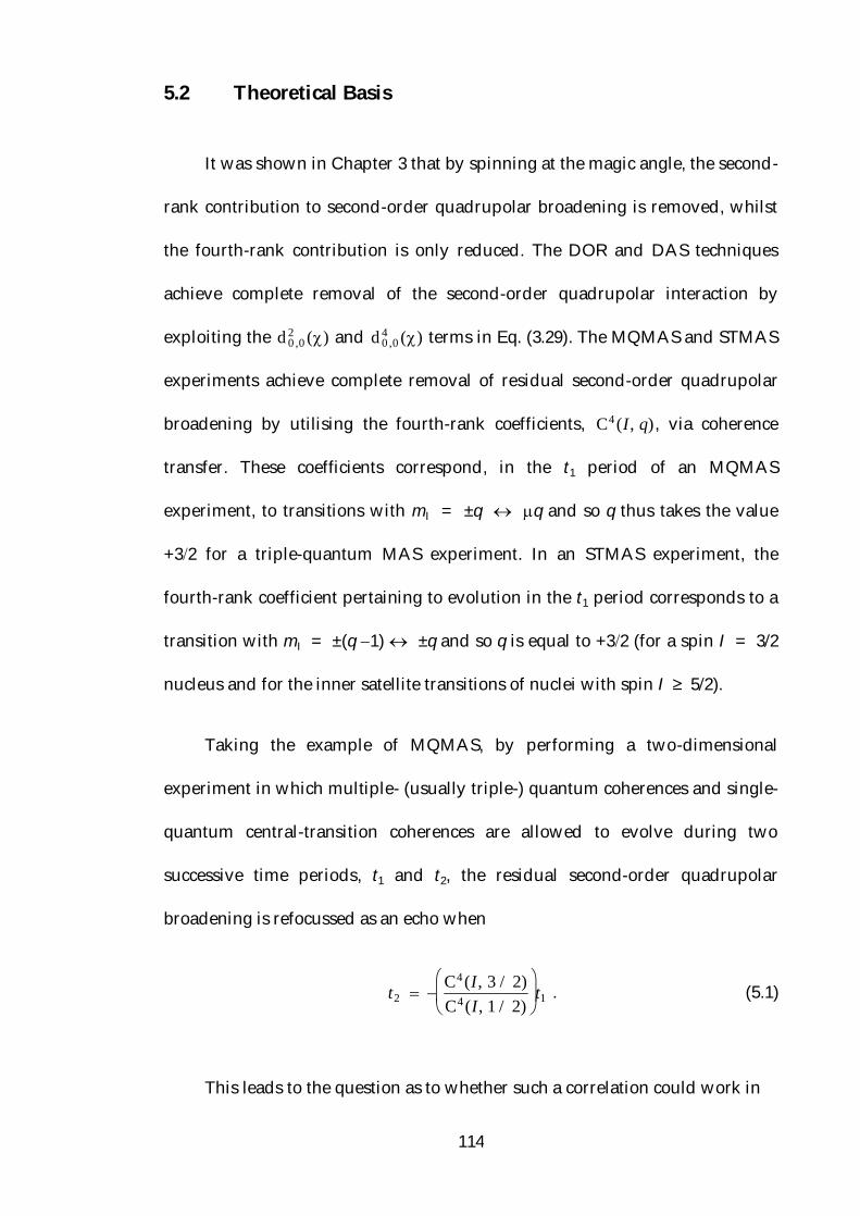
114
5.2 Theoretical Basis
It was shown in Chapter 3 that by spinning at the magic angle, the second-
rank contribution to second-order quadrupolar broadening is removed, whilst
the fourth-rank contribution is only reduced. The DOR and DAS techniques
achieve complete removal of the second-order quadrupolar interaction by
exploiting the d 0 ,02 () and d 0 ,0
4 () terms in Eq. (3.29). The MQMAS and STMAS
experiments achieve complete removal of residual second-order quadrupolar
broadening by utilising the fourth-rank coefficients, C4 (I, q), via coherence
transfer. These coefficients correspond, in the t1 period of an MQMAS
experiment, to transitions with mI = ±q q and so q thus takes the value
+32 for a triple-quantum MAS experiment. In an STMAS experiment, the
fourth-rank coefficient pertaining to evolution in the t1 period corresponds to a
transition with mI = ±(q 1) ±q and so q is equal to +32 (for a spin I = 32
nucleus and for the inner satellite transitions of nuclei with spin I ≥ 52).
Taking the example of MQMAS, by performing a two-dimensional
experiment in which multiple- (usually triple-) quantum coherences and single-
quantum central-transition coherences are allowed to evolve during two
successive time periods, t1 and t2, the residual second-order quadrupolar
broadening is refocussed as an echo when
t2
C4 (I, 3 / 2)C4 (I, 1 / 2)
t1 . (5.1)
This leads to the question as to whether such a correlation could work in

115
Figure 5.1. Energy-level diagram of a spin I = 32 nucleus demonstrating the interconversion
between p = 1 ST coherences and p = 2 DQ coherences achieved by the application of a CT-
selective 180 pulse.
real time. As in CPMG, in which a train of multiple echoes is acquired as a
function of a single time variable, an experiment comprising excitation of
multiple-quantum coherence and successive interconversion with central-
transition coherence could be envisaged. For such an experiment to be
successful, the pulses performing the excitation of triple-quantum coherences
and their conversion to central-transition coherences need to be highly efficient.
As shown in Chapter 4, both pulses are very inefficient, with the conversion
pulse being particularly poor. Consequently, performing such an experiment
would lead to a very large loss of signal intensity between successive echoes
and hence an intolerably large line-broadening in the isotropic spectrum.
It is known that central-transition-selective pulses are highly effective and
it has been reported that a selective inversion pulse applied to the central
transition leads to the transfer of the adjacent satellite-transition coherences
(±32 ±12) into double-quantum coherences (±32 12) with nearly 100%
efficiency [262]. This coherence transfer, illustrated in Fig. 5.1, has been
116
exploited in the DQF-STMAS and DQF-SATRAS techniques [262, 265].
Considering the C4 (I, q) coefficients of the satellite-transition and double-
quantum coherences of a spin I = 32 nucleus, these take the values 4835 and
+635, respectively. These coefficients are given in Appendix E; the latter is
obtained by a summation of the values for the central and satellite transitions
(5435 and 4835, respectively). This means that an experiment in which
selective central-transition conversion pulses are used for coherence transfer
between satellite and double-quantum transitions will lead to refocussing of the
residual second-order quadrupolar broadening for a spin I = 32 nucleus if the
periods of evolution are in the ratio 6:48 = 1:8. This is the principle of the
STARTMAS (satellite transitions acquired in real time MAS) experiment [266,
267], the details of which are given in the next section.
5.3 Pulse Sequence
The pulse sequence and coherence transfer pathway for the new
STARTMAS experiment are shown in Fig. 5.2. The first pulse is a hard pulse
optimized for excitation of satellite-transition coherences. Pairs of CT-selective
inversion pulses then interconvert the satellite-transition and double-quantum
coherences and, by spacing the pulses such that the periods of satellite-
transition and double-quantum evolution are in the ratio 1:8, the residual
second-order quadrupolar broadening is refocussed at the end of each period
(the STARTMAS cycle). The period is rotor-synchronized, = nR = nR and

117
Figure 5.2. Pulse sequence and coherence transfer pathway for the STARTMAS experiment for
spin I = 32 nuclei. The first two pulses are cycled with phase1 = 0, 45, 90, 135, 180, 225,
270, 315 and the receiver cycled with phase rx = 0, 90, 180, 270; this enables the
suppression of central-transition coherences excited by the first pulse [268]. The subsequent
180 pulses are cycled with phases 2 = 180 and 3 = 0, respectively.
this ensures that the first- and second-order quadrupolar interactions are
refocussed at the same point and that an isotropic echo is formed.
Consequently, data sampling with a period equal to will ensure removal of
quadrupolar broadening to second order. The number of rotor periods per
period, n, is usually chosen to be either 9 or 18, the effect of a variation of this
parameter is considered in Section 5.5.3. As in STMAS, the use of MAS to
remove the effects of the large first-order quadrupolar interaction dictates the
requirement for very accurate timings of the free precession intervals and,
consequently, a stable spinning speed and accurately adjusted spinning angle
are required. The excitation of central-transition coherences may occur, like in
STMAS, as an unwanted by-product of the initial pulse; however, judicious

118
Figure 5.3. Computer-simulated spin I = 32 isotropic STARTMAS NMR spectra illustrating
the spinor behaviour observed when the two inversion pulses in each STARTMAS unit are
applied with (a) the opposite phase and (b) the same phase.
phase cycling of the first two pulses and of the receiver is sufficient to remove
this [262, 265]. It should be noted that if the two CT-selective inversion pulses in
each STARTMAS unit are applied with the same radiofrequency phase then
alternate isotropic echoes are of opposite phase despite a net pulse flip angle of
360 being applied. This leads to an unwanted frequency shift of (R2n) Hertz
in the isotropic STARTMAS spectrum, as shown in Fig. 5.3, and is known as
spinor behaviour [268]. This property is not exhibited by central-transition
coherences, for which the application of two inversion pulses of the same phase
does not effect a sign change. This difference in behaviour of the central and
satellite transitions is a consequence of the former transition sharing two energy
levels with the transition across which the inversion pulses are being applied
and the latter only one. For satellite-transition coherences, the undesirable
frequency shift that arises from spinor behaviour may be circumvented by
applying two pulses with opposite phases, resulting in a net flip angle of 0.

119
5.4 Data Sampling Schemes
There are several data sampling schemes that may be envisaged for
STARTMAS, as illustrated in Fig. 5.4. Data points may be acquired by scheme
(i), in which data is sampled continuously throughout the experiment over the
wide spectral width needed for observation of spin I = 32 satellite transitions,
by scheme (ii), sampling over the same large spectral width but only during the
periods in which the satellite-transition signal is present and the first- and
second-order quadrupolar interactions are refocussed, or by scheme (iii),
sampling solely the points at the top of the isotropic echoes. Scheme (iii) yields
a spectrum with a much smaller spectral width than schemes (i) and (ii) that is
equal to the ratio of the MAS rate and the number of rotor periods in a period,
i.e., SW = Rn. These schemes are illustrated in Fig. 5.4, in which computer-
simulated time-domain signals and their Fourier transforms are shown.
As shown in Fig. 5.4a for the case of n = 18, scheme (i) produces a
truncated time-domain signal and this leads to a spectrum containing the
expected "sinc wiggles" [269]. Scheme (ii) yields a DOR-like spectrum
containing isotropic sidebands whose manifold is given by the static spin I =
32 satellite-transition lineshape (Fig. 5.4b). It should be noted that, if the
sideband spacing is given by SW = Rn, the spectral width is scaled by a factor
of x9, where x is the fraction of the satellite-transition acquisition window that
is sampled. As shown in Fig. 5.4c, scheme (iii) yields an isotropic spectrum [270]
that is devoid of sideband structure.

120
Figure 5.4. Computer-simulated time-domain and frequency-domain signals arising from four
possible STARTMAS data sampling schemes. (a) Scheme (i) produces a highly truncated time-
domain signal and spectrum. (b) Scheme (ii) yields a spectrum consisting of a series of isotropic
spinning sidebands. The satellite-transition centrebands are indicated by asterisks. (c) Scheme
(iii) yields an isotropic spectrum without a sideband manifold. (d) In scheme (iv) the whole
echoes in (b) are reordered into a two-dimensional array which upon Fourier transformation
yields an anisotropic-isotropic correlation spectrum. Spectra were simulated with the
parameters: 0 = 100 MHz, R = 33333 Hz, and in (b) and (d), x = 0.5. Two inequivalent sites
with 2 : 1 relative populations were simulated, with the parameters CQ = 1.6 MHz, = 0 and
CS = 1.0 ppm (site 1) and CQ = 2.0 MHz, = 0 and CS = 3.0 ppm (site 2). In the spectrum in
(d) contour levels are shown at 4, 8, 16, 32 and 64% of the maximum intensity.

121
Of the schemes described above, (ii) and (iii) appear to be the most useful.
Scheme (ii) enables the extraction of quadrupolar parameters from the envelope
of the spinning sideband pattern, whilst scheme (iii) benefits from the
sensitivity gain obtained when aliasing sideband intensity onto the satellite-
transitions centreband. Scheme (iv), shown in Fig. 5.4d, involves using the train
of echoes acquired in scheme (ii) to construct a two-dimensional array. This
scheme is, of course, not a different method of data sampling, but is rather a
different way of processing the data acquired using scheme (ii). The first
STARTMAS whole echo forms the first row of the two-dimensional dataset, the
second echo the second row, and so on. Two-dimensional Fourier
transformation of this time-domain signal then yields the two-dimensional
spectrum shown in Fig. 5.4d in which the static satellite-transition lineshape
appears in the F2 dimension (analogous to the 2 dimension defined in Section
2.7) and the isotropic spectrum in the F1 dimension (analogous to the 1
dimension defined in Section 2.7). This method of data sampling (essentially
analogous to methods reported for obtaining J spectra [271] and two-
dimensional one-pulse (TOP) spectra [272]) would seem to be the optimum
approach for acquiring STARTMAS NMR spectra, as it combines the
information found in the spectra yielded by schemes (ii) and (iii).
Whilst STARTMAS suppresses the first- and second-order quadrupolar
broadening, the isotropic chemical shift and second-order quadrupolar shift are
not refocussed. Consequently, the isotropic STARTMAS shift, that is, the
position of a given peak in the isotropic spectrum yielded by scheme (iii) and in

122
the F1 dimension of the two-dimensional spectrum shown in Fig. 5.4d, 1, is
given by:
1
179
CS 49Q , (5.2)
where CS is the isotropic chemical shift and Q is the quadrupolar shift,
[((QPAS )2 / 0 )(1 2 / 3)], expressed as a ppm shift.
In the isotropic dimension of an STMAS or MQMAS spectrum obtained
using either a shearing transformation, or by recording a split-t1 experiment,
both the isotropic chemical shift and quadrupolar shift are scaled. The isotropic
chemical shift is scaled by a factor, xCS, defined as [200]:
xCS
q R(I, q)1 R(I , q)
, (5.3)
where R(I, q) is the MQMAS (or STMAS) ratio defined in Chapter 3. The
coherence order of the transition evolving during the t1 period of MQMAS or
STMAS is again given by q and so takes the value ±32 for e.g., a triple-quantum
MAS experiment. The quadrupolar shift is scaled by a factor, xQ, given by [200]
),(R1
),(R))21,(A),(A( 00
Q qIqIIqI
x
. (5.4)
For a split-t1 STMAS experiment performed on a spin I = 32 nucleus, xCS
and xQ thus take the values 1 and 1017, respectively. Generally, these
123
quantities are related through the ratio
xCS
xQ
1710
. (5.5)
The chemical shift in the F1 dimension of a split-t1 MQMAS or STMAS
spectrum may be expressed in the form [53]
1 xCSCS A0 (I , 1 2)xQQ , (5.6)
and so, by comparison with Eq. (5.2), xCS and xQ thus have the values 179 and
109, respectively, for STARTMAS. The ratio xCSxQ is thus equal to 1710, the
same as is observed for MQMAS and STMAS. Consequently, the isotropic
spectra produced by STARTMAS are related by a simple scaling factor to those
obtained by MQMAS and STMAS.
5.5 Experimental Results
The results presented in this and the next section were processed using
MATLAB programs written by Dr M. J. Thrippleton. The simulated spectra
were also generated in MATLAB, by a stepwise integration of the Liouville-von
Neumann equation with a summation over 3722 orientations according to the
ZCW algorithm [273]. The spectra in Figs. 5.5a, 5.5b, 5.6, and 5.7 were recorded
with the assistance of Dr S. Steuernagel (Bruker Biospin GmbH, Rheinstetten,
Germany).

124
5.5.1 STARTMAS at High MAS Rates
STARTMAS NMR data were acquired at high spinning rates for four
powdered solids, namely sodium oxalate, Na2C2O4, sodium citrate dihydrate,
Na3C6H5O7·2H2O, dibasic sodium phosphate, Na2HPO4, and rubidium nitrate.
RbNO3. Time-domain signals acquired with 87Rb STARTMAS NMR of
rubidium nitrate and 23Na STARTMAS NMR of sodium citrate dihydrate are
shown in Figs. 5.5a and 5.5b, along with their corresponding Fourier transforms
(Figs. 5.5c and 5.5d), respectively. The one-dimensional DOR-like spectra
shown in Figs. 5.5c and 5.5d have the expected appearance, consisting of an
array of spinning sidebands which, for each crystallographically inequivalent
site present in each solid (three in both rubidium nitrate [221] and sodium
citrate dihydrate [164]), have an envelope corresponding to the static satellite-
transition first-order quadrupolar broadened lineshape. It should be noted that
in Fig. 5.5c, two of the sites in rubidium nitrate are coincident at this magnetic
field strength due to the combined effect of the isotropic chemical shift and the
second-order quadrupolar shift. The areas of intensity that fall below the
baseline in Figs. 5.5c and 5.5d are consistent with the zero total integral of these
spectra, this being a consequence of pulse-ringdown effects that preclude
acquisition of the first half echo and so lead to a zero first point. Inspection of
Figs. 5.5c and 5.5d reveals that the spinning sidebands are not spaced by the
spinning speed, 33333 Hz. Owing to the non-continuous data sampling (points
are collected only during part of the satellite-transition acquisition window),
the sideband spacing is scaled by a factor 12x (where x is the fraction of the

125
Figure 5.5. Time-domain data acquired using (a) 87Rb STARTMAS NMR of rubidium nitrate
and (b) 23Na STARTMAS NMR of sodium citrate dihydrate and the corresponding one-
dimensional spectra (c) and (d), respectively. Experiments were performed at B0 = 11.7 T and a
MAS rate of 33333 Hz. The n = 18 STARTMAS condition was used with x = 0.133, and 1584
and 1024 transients were averaged for rubidium nitrate and sodium citrate dihydrate,
respectively. The initial excitation pulse had duration in the range 1.2–1.5 s and the selective
inversion pulses had duration 20 s. Computer-simulated spectra in (e) and (f) were generated
using literature NMR parameters [53, 164] for rubidium nitrate and sodium citrate dihydrate,
respectively. The centrebands are indicated by asterisks.
satellite-transition acquisition window that is sampled, defined previously in
Section 5.4), such that the separation of the sidebands is now 125 kHz. The
computer-simulated spectra shown in Figs. 5.5e and 5.5f broadly agree with the
experimental data.

126
It should be noted that the spectra in Figs. 5.5c–f are poorly suited to
quantitative analysis, as a consequence of the baseline dip that results from the
zero first point in the time domain data in Figs. 5.5a and 5.5b. This may be
circumvented by a left shift of the time-domain data such that it begins at the
top of the first whole echo. After one-dimensional Fourier transformation a
large first-order phase correction is required, but this can easily be performed.
This yields a spectrum like that shown in Fig. 5.4b, although the spectrum
shown there was simulated by making the (experimentally unrealistic)
assumption of infinitely short pulses, such that the first half echo could be
acquired.
Figure 5.6 presents the two-dimensional 87Rb STARTMAS NMR spectra of
rubidium nitrate, generated by Fourier transformation of data acquired using
the scheme shown in Fig. 5.4d. The simulated spectrum in Fig. 5.6a matches
well the experimental spectrum in Fig. 5.6c, where the two coincident sites are
seen to be partly aliased. Projections along the F1 dimension of each spectrum
are shown in Figs. 5.6b and 5.6d, where the isotropic spectral width equals R18
= 1852 Hz. The three crystallographically inequivalent sites in rubidium nitrate
have the quadrupolar parameters [53]: CQ = 1.70 MHz, = 0.6, CQ = 1.70
MHz, = 0.2 and CQ = 2.00 MHz, = 0.9 and are labelled 1, 2 and 3 in Fig.
5.6, respectively. The corresponding peaks of each site in the isotropic spectra
have intensities that are consistent with their 1 : 1 : 1 population ratio [221].
Two-dimensional 23Na STARTMAS NMR spectra of sodium citrate
dihydrate are shown in Fig. 5.7, obtained via the data sampling scheme in Fig.

127
Figure 5.6. (a) Computer-simulated and (c) experimental two-dimensional 87Rb STARTMAS
NMR spectra of rubidium nitrate. The spectrum in (a) was generated using literature NMR
parameters [53] and (c) was obtained from the one-dimensional time-domain data in Fig. 5.5a.
The asterisked peak is present as a consequence of imperfections associated with the
experimental implementation. Corresponding F1 projections are shown in (b) and (d). Contour
levels in (a) and (c) are shown at 20, 35, 50, 65, 80 and 95% of the maximum intensity.
5.4d. The three inequivalent 23Na sites present in this material are seen to be
well-resolved in the F1 projections in Figs. 5.7b and 5.7d and have values of the
quadrupolar product, PQ [107], equal to 1.87 MHz, 1.65 MHz and 1.90 MHz for
sites 1, 2 and 3, respectively [274]. As in rubidium nitrate, the relative peak
intensities concur well with the 1 : 1 : 1 population ratio [164] for the three sites
in the solid.

128
Figure 5.7. (a) Computer-simulated and (c) experimental two-dimensional 23Na STARTMAS
NMR spectra of sodium citrate dihydrate. The spectrum in (a) was generated using literature
NMR parameters [274] and (c) was obtained from the one-dimensional time-domain data in Fig.
5.5b. Contour levels in (a) and (c) are shown at 20, 35, 50, 65, 80 and 95% of the maximum
intensity. The "spike" marked with an asterisk arises due to imperfections in the experimental
implementation. Corresponding F1 projections are shown in (b) and (d).
23Na STARTMAS NMR spectra of sodium oxalate and dibasic sodium
phosphate were also acquired and are shown in Figs. 5.8a and 5.8c,
respectively. The two-dimensional spectra and corresponding F1 projections
shown in Figs. 5.8b and 5.8d are consistent with the presence of one [275] and
three [276] inequivalent sites, respectively. The three inequivalent sites in
dibasic sodium phosphate have CQ values of 3.8, 1.3 and 2.0 MHz for sites, 1, 2
and 3, respectively [248]. The odd F1 chemical shift scale in Figs. 5.8c and 5.8d

129
Figure 5.8. Two-dimensional 23Na (n = 18) STARTMAS NMR spectra of (a) sodium oxalate and
(c) dibasic sodium phosphate. Spectra were acquired at B0 = 9.4 T and a MAS rate of (a) 30000
Hz and (c) 28125 Hz, so leading to isotropic spectral widths equal to 1666 Hz and 1562 Hz,
respectively. F1 projections are shown in (b) and (d). Satellite-transition excitation pulses of 2.0–
2.2 s were used and the CT-selective pulses had duration 30 s. Contour levels in (a) and (c)
are shown at 20, 35, 50, 65, 80 and 95% of the maximum intensity.
arises as a consequence of one of the peaks being at the edge of the spectral
width such that half of it is aliases. Rearranging the spectrum in this way
enables the 3 sites to be clearly seen.
It was shown in Chapter 4 that, for the case ofMQMAS, the efficiency of
both the excitation and conversion pulses varies with Q. STMAS shows a
similar, although less pronounced, variation in signal intensity with CQ [53]

130
and, like MQMAS, is a non-quantitative technique. This has been illustrated
using dibasic sodium phosphate, where the intensity ratio 1.1 : 1.0 : 0.7
(observed in STMAS) and 0.4 : 1.0 : 0.5 (in MQMAS) [53] does not concur with
the 2 : 1 : 1 relative site population predicted from the crystal structure [275].
The F1 projection of dibasic sodium phosphate shown in Fig. 5.8d reveals that
the three sites yield peaks in the approximate intensity ratio 0.8 : 1.0 : 0.9. Given
that STARTMAS involves the excitation of satellite-transition coherences, the
similarity of this ratio to that obtained using STMAS is not surprising.
5.5.2 Ultrafast STARTMAS NMR
Under conditions of high sensitivity, such as at very high static magnetic
fields or with large sample volumes, STARTMAS may be described as
"ultrafast". In contrast to two-dimensional methods like MQMAS and STMAS,
STARTMAS is not limited by data sampling requirements (such as that of the t1
period in the former two techniques) and so is limited only by sensitivity
considerations. To demonstrate the ability of STARTMAS to produce ultrafast
spectra, 87Rb STARTMAS NMR spectra of rubidium nitrate were recorded
using a 4.0-mm MAS probe to maximise sample volume. As the achievable
spinning speeds are much lower on this probe than on the 2.5-mm probe used
for obtaining the spectra in Figs. 5.5–5.7, the n = 9 condition was used to
maximise the isotropic spectral width. The two-dimensional spectra and
corresponding F1 projections are shown in Fig. 5.9 with that in Fig. 5.9a

131
Figure 5.9. Two-dimensional 87Rb STARTMAS NMR spectra of rubidium nitrate recorded at B0
= 9.4 T with (a) 1024 transients and (c) 1 transient. The MAS rate was 14286 Hz and the n = 9
STARTMAS condition was used, so producing an isotropic spectral width of 1587 Hz. Inversion
pulses of 30 s were used and the satellite-transition excitation pulse had duration 1.8 s.
Corresponding F1 projections are shown in (b) and (d), where the 3 sites are indicated by
asterisks. Contour levels in (a) and (c) are shown at 15, 25, 45, and 85% of the maximum
intensity.
recorded with 1024 transients and that in Fig. 5.9c recorded with a single
transient. The spectrum in Fig. 5.9a reveals the expected three sites (labelled 1, 2
and 3, in the same way as in Fig. 5.6) present in rubidium nitrate (two of them
no longer being coincident due to the experiment being performed at a different
magnetic field strength than in Figs. 5.5 and 5.6). In Fig. 5.9c, these two sites
again appear as one peak, this being due to the line broadening resulting from
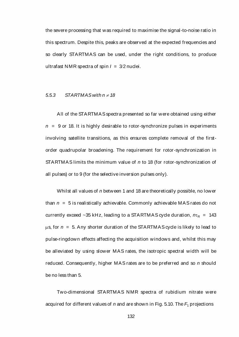
132
the severe processing that was required to maximise the signal-to-noise ratio in
this spectrum. Despite this, peaks are observed at the expected frequencies and
so clearly STARTMAS can be used, under the right conditions, to produce
ultrafast NMR spectra of spin I = 32 nuclei.
5.5.3 STARTMAS with n 18
All of the STARTMAS spectra presented so far were obtained using either
n = 9 or 18. It is highly desirable to rotor-synchronize pulses in experiments
involving satellite transitions, as this ensures complete removal of the first-
order quadrupolar broadening. The requirement for rotor-synchronization in
STARTMAS limits the minimum value of n to 18 (for rotor-synchronization of
all pulses) or to 9 (for the selective inversion pulses only).
Whilst all values of n between 1 and 18 are theoretically possible, no lower
than n = 5 is realistically achievable. Commonly achievable MAS rates do not
currently exceed ~35 kHz, leading to a STARTMAS cycle duration, nR = 143
s, for n = 5. Any shorter duration of the STARTMAS cycle is likely to lead to
pulse-ringdown effects affecting the acquisition windows and, whilst this may
be alleviated by using slower MAS rates, the isotropic spectral width will be
reduced. Consequently, higher MAS rates are to be preferred and so n should
be no less than 5.
Two-dimensional STARTMAS NMR spectra of rubidium nitrate were
acquired for different values of n and are shown in Fig. 5.10. The F1 projections

133
Figure 5.10. 87Rb STARTMAS NMR spectra of rubidium nitrate, acquired using different values
of n. (a) F1 projection of the STARTMAS spectra recorded using (a) n = 9 and (b) n = 18. (c)
Two-dimensional spectrum recorded with n = 5 and (d) the corresponding F1 projection. The
spectra were obtained at B0 = 9.4 T, using MAS rates of (a) 14286 Hz, (b) 30000 Hz and (c) 7937
Hz. CT-selective pulses of duration 30 s were used and the satellite-transition excitation pulse
had duration 2.0–2.2 s. Contour levels in (c) are shown at 20, 35, 50, 65, 80 and 95% of the
maximum intensity.
obtained from the spectra acquired using n = 9 and 18 are shown in Figs. 5.10a
and 5.10b, respectively. These two conditions, corresponding to complete (n =
18) and partial (n = 9) rotor-synchronization lead to isotropic STARTMAS
spectra of comparable resolution and linewidths. The n = 9 condition appears
to resolve the two 87Rb sites that have very similar positions in the F1
dimension, whilst in the n = 18 case, these two sites are not separated. There is

134
no obvious reason for this differing resolution, other than the different
characteristics of the 2 different probes used for acquiring the n = 9 and n = 18
data. In both cases, good signal-to-noise ratios are obtained and peaks appear at
the expected positions, so clearly, using either n = 9 or 18 is an acceptable way
of recording STARTMAS spectra. In Fig. 5.10c, however, the spectrum acquired
using n = 5 possesses a worse signal-to-noise ratio than the n = 9 and 18
spectra. This is clearly seen in the projection in Fig. 5.10d, where much broader
and more distorted lineshapes are observed. It would thus seem that the
performance of STARTMAS is optimum when rotor-synchronization (n = 9 or
18) is used.
5.5.4 Extraction of Quadrupolar Parameters
As is the case for MQMAS and STMAS, F2 projections of two-dimensional
STARTMAS spectra yield lineshapes whose width and shape are indicative of
the size and asymmetry of the quadrupolar tensor. In contrast to MQMAS and
STMAS, where the lineshapes typically have widths ~kHz, those obtained from
STARTMAS are usually ~MHz wide. Consequently, F2 lineshapes obtained
from STARTMAS spectra are susceptible to probe bandwidth distortions and so
quadrupolar parameters obtained using this method are likely to be less
accurate than those obtained using other methods.
F2 lineshapes extracted from the two-dimensional 87Rb STARTMAS NMR
spectrum of rubidium nitrate from which the F1 projection in Fig. 5.10b was
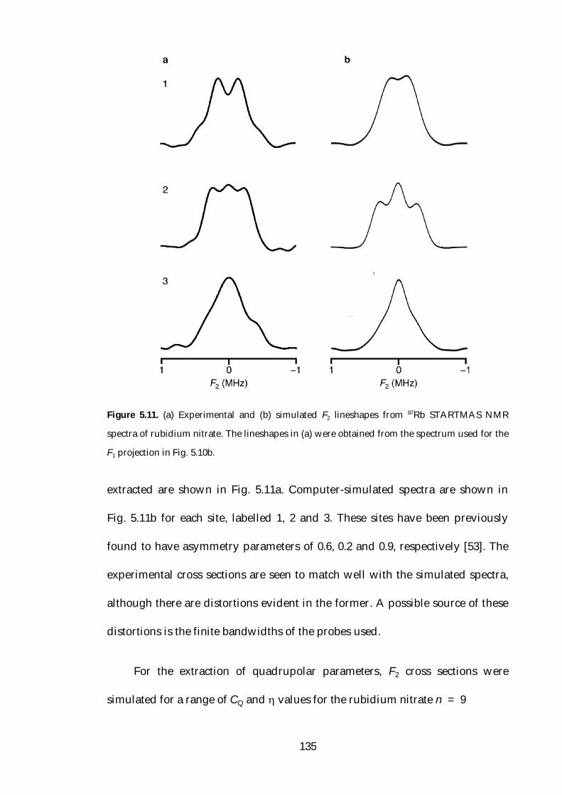
135
Figure 5.11. (a) Experimental and (b) simulated F2 lineshapes from 87Rb STARTMAS NMR
spectra of rubidium nitrate. The lineshapes in (a) were obtained from the spectrum used for the
F1 projection in Fig. 5.10b.
extracted are shown in Fig. 5.11a. Computer-simulated spectra are shown in
Fig. 5.11b for each site, labelled 1, 2 and 3. These sites have been previously
found to have asymmetry parameters of 0.6, 0.2 and 0.9, respectively [53]. The
experimental cross sections are seen to match well with the simulated spectra,
although there are distortions evident in the former. A possible source of these
distortions is the finite bandwidths of the probes used.
For the extraction of quadrupolar parameters, F2 cross sections were
simulated for a range of CQ and values for the rubidium nitrate n = 9
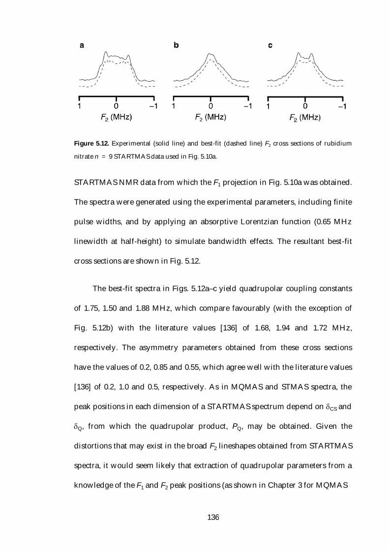
136
Figure 5.12. Experimental (solid line) and best-fit (dashed line) F2 cross sections of rubidium
nitrate n = 9 STARTMAS data used in Fig. 5.10a.
STARTMAS NMR data from which the F1 projection in Fig. 5.10a was obtained.
The spectra were generated using the experimental parameters, including finite
pulse widths, and by applying an absorptive Lorentzian function (0.65 MHz
linewidth at half-height) to simulate bandwidth effects. The resultant best-fit
cross sections are shown in Fig. 5.12.
The best-fit spectra in Figs. 5.12a–c yield quadrupolar coupling constants
of 1.75, 1.50 and 1.88 MHz, which compare favourably (with the exception of
Fig. 5.12b) with the literature values [136] of 1.68, 1.94 and 1.72 MHz,
respectively. The asymmetry parameters obtained from these cross sections
have the values of 0.2, 0.85 and 0.55, which agree well with the literature values
[136] of 0.2, 1.0 and 0.5, respectively. As in MQMAS and STMAS spectra, the
peak positions in each dimension of a STARTMAS spectrum depend on CS and
Q, from which the quadrupolar product, PQ, may be obtained. Given the
distortions that may exist in the broad F2 lineshapes obtained from STARTMAS
spectra, it would seem likely that extraction of quadrupolar parameters from a
knowledge of the F1 and F2 peak positions (as shown in Chapter 3 for MQMAS

137
and STMAS) is a preferable method to the fitting procedure shown in Fig. 5.12.
5.6 Applications of STARTMAS
5.6.1 Isotropic-Isotropic Correlation
There have been several reports in the literature of experiments that
enable connectivity information for quadrupolar nuclei in the solid state to be
obtained [127, 277–281]. Magnetization transfer between inequivalent sites can
provide site-specific information and this has enabled the relative orientation of
quadrupolar tensors to be obtained via two-dimensional triple-quantum
NOESY experiments [277, 280]. In addition, MQMAS has been incorporated
into three-dimensional experiments and CSA and dipolar coupling parameters
have been obtained [279]. The experiments detailed in Refs. [277–280] yield
spectra in which there is an absence of anisotropic broadening (CSA, dipolar or
quadrupolar in origin) in only one dimension. In Refs. [127] and [281], however,
a two-dimensional correlation experiment derived from DOR is introduced that
produces a spectrum that is isotropic in both dimensions. This is useful in cases
where the overlap of peaks from inequivalent sites can limit the information
that may be obtained from correlation spectra. Given the fact that STARTMAS
can, like DOR, produce isotropic spectra in real time, a homonuclear correlation
experiment derived from STARTMAS could thus prove a useful technique for
establishing connectivities between quadrupolar nuclei in the solid state. Such
an experiment would also not be hindered by the technical requirements that
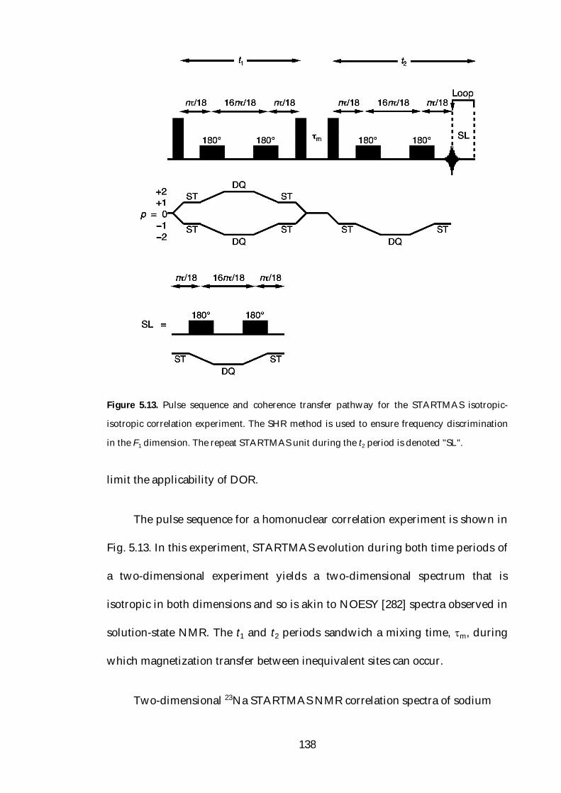
138
Figure 5.13. Pulse sequence and coherence transfer pathway for the STARTMAS isotropic-
isotropic correlation experiment. The SHR method is used to ensure frequency discrimination
in the F1 dimension. The repeat STARTMAS unit during the t2 period is denoted "SL".
limit the applicability of DOR.
The pulse sequence for a homonuclear correlation experiment is shown in
Fig. 5.13. In this experiment, STARTMAS evolution during both time periods of
a two-dimensional experiment yields a two-dimensional spectrum that is
isotropic in both dimensions and so is akin to NOESY [282] spectra observed in
solution-state NMR. The t1 and t2 periods sandwich a mixing time, m, during
which magnetization transfer between inequivalent sites can occur.
Two-dimensional 23Na STARTMAS NMR correlation spectra of sodium

139
citrate dihydrate are shown in Fig. 5.14, recorded using the pulse sequence in
Fig. 5.13. 1H decoupling was applied during the t1 and t2 periods, but not
during the mixing time, so as to enable proton-driven spin diffusion [283] to
occur between the 23Na nuclei. The spectrum in Fig. 5.14a, recorded with a zero
mixing time, shows the expected 3 diagonal peaks for the 3 inequivalent sites in
this material. In Fig. 5.14b, where the mixing time is 245 ms, there appears to be
a cross peak between the two lowest frequency sites. F2 cross sections taken at
the F1 frequency of this cross peak are shown alongside the spectra in Figs.
5.14a–d. It should be noted that these cross sections are not shown with the
correct relative intensities; these have been adjusted so that the diagonal peak
intensity appears constant and so that any changes in cross peak intensity may
be more clearly observed. There is, of course, a significant loss of intensity
between the experiments in Fig. 5.14a and 5.14d due to 23Na T1 relaxation.
The spectra in Fig. 5.14c and 5.14d, acquired at mixing times of 490 ms and
980 ms, respectively, reveal a continual growth in cross peak signal intensity,
although in Fig. 5.14d this peak has an intensity not much greater than the
background noise signal. A cross peak partner at a position obtained by
reflection about the diagonal spectral axis is virtually absent, until the spectrum
in Fig. 5.14d, where it appears with much lesser intensity. This feature is
unsurprising if the intensity of the diagonal peaks in Fig. 5.14a is considered.
The diagonal peak shown in the F2 cross sections alongside Figs. 5.14a–d has
much greater intensity than that arising from the 2 other sites in sodium citrate
dihydrate, this of course being a consequence of the non-quantitative nature of

140
Figure 5.14. Two-dimensional 23Na STARTMAS NMR correlation spectra of sodium citrate
dihydrate recorded with a mixing time of (a) 0, (b) 245 ms, (c) 490 ms and (d) 980 ms. Alongside
each spectrum is the F2 cross section corresponding to the most intense diagonal peak. All
experiments were performed at B0 = 9.4 T, a MAS rate of 14286 Hz and with n = 9. The CT-
selective, satellite-transition excitation and z-filter pulses had duration 30 s, 2.0 s and 2.0 s,
respectively. Contour levels in (a–d) are shown in 10% increments in the range of 5–95% of the
maximum intensity.
141
satellite-transition excitation. Given that the intensity of the cross peaks is
dependent on the amount of magnetization present at the end of the t1 period
on the spin from which the magnetization was transferred during the mixing
time, the greater intensity of cross peaks arising from transfer from the spin
yielding the most intense diagonal peak is not surprising.
This experiment was repeated on rubidium nitrate and sodium
metasilicate pentahydrate, Na2SiO3·5H2O, (results not shown). No cross peaks
were observed for rubidium nitrate; this is most likely a consequence of (i) the
relatively short T1 relaxation times in this material (less than 200 ms for all 3
sites), (ii) the 40% natural abundance of 87Rb nuclei that increases the average
distance between adjacent 87Rb nuclei and (iii) the absence of 1H nuclei that
removes the possibility of enhanced spin diffusion between 87Rb nuclei. In
sodium metasilicate pentahydrate, for which exchange peaks between the two
inequivalent sites have been reported previously [280], a pair of cross peaks
was observed. As in the case of sodium citrate dihydrate, a significant disparity
in the intensity of the cross peaks was observed, this most likely being
attributable once again to the non-quantitative nature of satellite-transition
excitation.
Reports of magnetization transfer between quadrupolar nuclei have
generally yielded cross peaks of low intensity [277–280], although the absence
of anisotropic broadening in correlation spectra obtained using STARTMAS
would suggest that any cross peaks observed would have greater relative
intensity. The spectra shown in Fig. 5.14 do not confirm this view, although

142
they do demonstrate the ease with which isotropic-isotropic correlation spectra
may be obtained. In the absence of real-time data acquisition, such spectra may
only be obtained via three-dimensional experiments, which, in many cases, may
require a prohibitively long duration.
5.7 Conclusions
The new STARTMAS experiment has been shown to produce isotropic
spectra of spin I = 32 nuclei in real time; this could only previously be
achieved using specialist DOR probes. STARTMAS has been demonstrated on a
range of powdered solids and, in cases of high sensitivity, spectra may be
obtained using very few transients, or even just a single transient. It has been
shown that STARTMAS can be performed at any value of n ≥ 5 but, for
optimum results, the n = 9 or 18 conditions should be used. In addition,
lineshape fitting procedures have been used to demonstrate the utility of
STARTMAS spectra in obtaining quadrupolar parameters, although the
susceptibility of the lineshapes to distortions due to probe and filter bandwidth
effects means that such parameters are likely to be less reliable than those
obtained by other means. The ability of STARTMAS to produce isotropic-
isotropic correlation spectra has been shown and this application of the
technique would appear to offer much promise.
One of the greatest challenges remaining for STARTMAS is to extend the
method to spin I = 52 nuclei. The fourth-rank coefficients, A4(I, q), for the

143
inner satellite (mI = ±12 ±32) and inner double-quantum (mI = ±32
12) transitions of all nuclei with spin I > 32 are of the same sign and so the
current approach to STARTMAS will fail in such cases. For nuclei with spin I >
32, interconversion of satellite and double-quantum coherences of opposite
sign is thus needed. There are currently no known pulse schemes that can
perform this conversion with the high efficiency required for real-time data
acquisition.
The isotropic spectral width obtained in STARTMAS is small compared to
that typically seen in MQMAS and STMAS spectra. This can, in many cases,
lead to considerable aliasing and unwanted peak overlap may occur. Another
improvement which would prove useful for STARTMAS is thus an increase in
spectral width, which is constrained by the spinning frequency, the length of
the selective pulses and the rotor-synchronization requirements. Finally, the use
of MAS probes with larger bandwidths would enable extraction of F2
lineshapes that are a more accurate reflection of the quadrupolar tensors
characterising the satellite transitions.

144
Chapter 6
NOE Studies of Borane Adducts
6.1 Introduction
The nuclear Overhauser effect (NOE) [59, 61] is one of the most widely
exploited phenomena in NMR and is well known as a means of determining
molecular structure in solution. The effect arises through cross-relaxation
driven by the modulation of the dipolar interaction between two spatially
proximate spins, conventionally labelled I and S. Upon perturbation of the
populations of the S-spin energy levels, cross-relaxation processes act to return
the populations of the energy levels to their equilibrium values. This has the
simultaneous effect of altering the population differences across the I-spin
transitions, so leading to the observed increase or decrease in I-spin signal
intensity.
Modulation of the dipole-dipole interaction arises due to the presence of
molecular motion on the correct timescale. In the solution state, this motion
exists as a result of the rapid, random tumbling. In the solid state, such motion
is rarely observed due to the structural rigidity imposed on the molecules and
consequently NOEs are typically not observed. The exceptions to this have
mainly been in polymeric hydrocarbon derivatives, where the rapid rotation of
methyl groups about their C3 axes leads to 13C{1H} NOEs [64–66], and in the

145
case of adamantane and other "plastic crystals", where modulation of the
heteronuclear dipolar interaction by isotropic molecular tumbling leads to
enhancement of the 13C signal intensity.
NOEs to quadrupolar nuclei are rarely observed, this being due to the
typically much greater efficiency of quadrupolar relaxation than dipolar cross-
relaxation. Given that quadrupolar spin-lattice relaxation is proportional to the
square of CQ, solution-state NOEs are only likely to be observed for nuclei with
small quadrupole moments (e.g., 2H and 6Li, both with spin I = 1), or for
quadrupolar nuclei in highly symmetric environments. Reports of NOEs to
quadrupolar nuclei have been mainly confined to 6Li [67, 284, 285] and 7Li (spin
I = 32) [286] nuclei.
Unusually, the presence of a 11B{1H} transient NOE in solid borane
triphenylphosphine, BH3·PPh3, has recently been reported in an MAS NMR
experiment [287]. The existence of an NOE in this case has been attributed to
the presence of rapid rotation of the BH3 group about its C3 axis that modulates
the 11B{1H} dipolar interaction. The absence of strong quadrupolar relaxation in
this case is most likely due to the coincidence of the 11B quadrupolar tensor and
the C3 symmetry axis. This has the effect that rotation of the BH3 group leads to
very little modulation of the 11B quadrupolar interaction and thus inefficient
quadrupolar relaxation.
In this chapter, 11B{1H} NOE results are presented for a series of borane
adducts. 11B{1H} transient NOE experiments are used to obtain 11B NMR
146
enhancements in a range of phosphine- and amine-derived borane adducts
under MAS conditions and the results are compared and a rationale proposed
for the trends seen. The 11B{1H} enhancement of the 11B satellite transitions is
obtained and a triple-quantum filtered transient NOE experiment is used for
the analogous measurement for the 11B triple-quantum transition. Variable-
temperature NMR results are presented that demonstrate the variation of the
11B{1H} NOE enhancement in borane triphenylphosphine and the results
obtained are considered in terms of the measured spin-lattice relaxation times
and with the aid of theoretical calculations. A comparison of the NOE
enhancements observed under static and MAS conditions is also made and
theoretical arguments are used to rationalise the behaviour in the former case.
6.2 Theory
6.2.1 The Heteronuclear NOE
The nuclear Overhauser effect may be explained simply by considering
the nuclear spin energy levels involved. Take, for example, the case of a
heteronuclear IS dipolar-coupled spin pair, where I = 13C (spin I = 12) and S
= 1H (spin I = 12). The energy levels of such a system are shown in Fig. 6.1,
where the numbers shown above each energy level signify the relative
deviations of their populations from a fully saturated state by assuming that
SI = 4. Shown in Fig. 6.1a are the energy levels at thermal equilibrium with
the I- and S-spin transitions indicated. In Fig. 6.1b the energy levels are shown

147
Figure 6.1. Energy levels of an IS heteronuclear spin pair for the case where I = 13C and S = 1H, depicted at (a) thermal equilibrium, (b) after inversion of the populations of the S-spin
energy levels and (c) after cross-relaxation via the double-quantum (W2IS) pathway has restored
the population difference between the energy levels indicated.
for the case where the populations of the S-spin energy levels are inverted (as in
a transient NOE experiment). After perturbation of the populations of the S-
spin energy levels, which leaves the population difference across the I-spin
transitions unaffected, relaxation pathways act to return the populations of
certain energy levels to their equilibrium values, as indicated in Fig. 6.1b. The
W1I and W1
S pathways correspond to a transition between the I- and S-spin
energy levels, respectively, with the one subscript indicating that the transition
involves a net change of magnetic quantum number, mI, of one. Relaxation
via this pathway simply corresponds to spin-lattice relaxation of the I and S
148
spins and so leads to the energy levels being populated as in Fig. 6.1a. There are
two other pathways that can restore populations of the energy levels and these
are denoted W0IS and W2
IS, as they involve a net change in magnetic quantum
number of zero and two, respectively. Relaxation via these pathways is known
as cross-relaxation as it involves a simultaneous change of the populations of
the energy levels of both spins. By restoring the populations of the energy levels
indicated to their equilibrium values, relaxation via these two pathways leads
to a simultaneous change of the population difference across the I-spin
transitions. This is shown in Fig. 6.1c, where the populations of the energy
levels are shown after hypothetical cross-relaxation solely via the W2IS pathway
has occurred. It is shown that the population difference across the I-spin
transitions, nI, has increased to 10 from its value of 2 at thermal
equilibrium. This increase in I-spin signal intensity is referred to as the NOE
enhancement. The effect of cross-relaxation via the zero-quantum, W0IS
pathway is not indicated in Fig. 6.1. This is because, for small molecules in
solution, this pathway makes a very small contribution to cross-relaxation. This
will be explained further in the next section.
6.2.2 The Solomon Equations
It was shown by Solomon [61] that the behaviour of the I- and S-spin
magnetizations after perturbation of the populations of the S-spin energy levels
may be expressed using the following rate equations:

149
0SI0S
0IS0I
I)(IS)(Sd
)(Sd
S)(SI)(Id
)(Id
zzzzz
zzzzz
ttt
t
ttt
t
. (6.1)
where Iz (t ) and Sz (t ) are ensemble averages of the expectation values of the
z-components of the spin angular momentum operators at time t of the I and S
spins, respectively. 0I z and 0S z are the expectation values of the same
operators at equilibrium. Equation (6.1) is often simplified such that the
expectation value and ensemble average are implied, which yields:
0SI
0S
0IS
0I
I)(IS)(Sd
)(dS
S)(SI)(Id
)(dI
zzzzz
zzzzz
ttt
t
tttt
, (6.2)
where 0Iz = 0I z and 0S z = 0S z . Equation (6.2) would seem to imply that
the operators are time dependent. This of course is not the case, as it is actually
the populations and wavefunctions of the spin systems that are changing.
In Eqs. (6.1) and (6.2) the cross-relaxation rate constant is denoted IS,
whilst the self-relaxation rate constants for the I and S spins are given by I and
S, respectively. These equations show that the behaviour of the I- and S-spin
magnetizations is dependent on both the spin-lattice relaxation of each spin,
and on the cross-relaxation. Note that the term involving is directly
proportional to the change in the magnetization of the coupled spin in each case
— this shows that the evolution of the I-spin magnetization is dependent on the

150
perturbation of the S-spin magnetization (and vice versa) and so is an
equivalent way of describing what was shown in Fig. 6.1.
In the transient NOE experiment, shown in Fig. 6.2, the populations of the
S-spin energy levels are inverted by the application of a 180 pulse to the S
spins. Cross-relaxation then occurs during the NOE build-up interval, , before
a 90 pulse on the I spin excites I-spin single-quantum coherence. The
experiment is repeated using different values of and the change in I-spin
signal intensity is observed. In such an experiment, directly after the S-spin
inversion pulse ( = 0) the I- and S-spin magnetizations take the values:
Iz (0) Iz0
Sz (0) Sz0 . (6.3)
If the approximation is made that the I- and S-spin magnetizations take
the values given in Eq. (6.3) (the initial rate approximation), then these
boundary conditions may be used to obtain the following behaviour of the I-
spin magnetization, where t is now replaced by :
dI z ()
d 2ISSz
0 , (6.4)
which yields the following solution:
Iz () 2 ISSz0 Iz
0 . (6.5)
Equation (6.4) states that the I-spin magnetization is dependent on and on the

151
cross-relaxation rate constant IS, the latter of course being responsible for the
NOE.
The behaviour of the S-spin magnetization may also be obtained by
solving the second part of Eq. (6.1), which yields the equation:
Sz () 2SSz0 Sz
0 . (6.6)
The S-spin magnetization thus returns to its equilibrium value at a rate
characterised by its self-relaxation rate constant.
Using Eq. (6.5), an NOE enhancement, , is defined as:
I
SIS
0
0IS
0
0
2
IS2
II)(I
z
z
z
zz
. (6.7)
Given that is directly proportional to the gyromagnetic ratio of the S spin, this
nucleus is typically chosen to be high-, i.e., 1H or 19F.
Equations (6.1–6.7) are only valid in the initial rate approximation, in
which the NOE does not reach its maximum, and the conditions IS << 1 and
S << 1 are satisfied. At longer mixing times, the solutions of Eq. (6.1) are
more difficult to obtain, but nevertheless, the following expressions may be
obtained for the time dependence of the I- and S-spin magnetizations, assuming

152
Figure 6.2. Pulse sequence and coherence transfer pathway for the transient NOE experiment
that measures the heteronuclear NOE enhancement experienced by the central transition of spin
I upon inversion of the populations of the S-spin energy levels. The NOE build-up interval is
denoted .
that IS = SI (an assumption that holds when the spin quantum numbers of
the I and S spins are equal) [288]:
Iz () Iz0
2ISIz0S
AIexp( C 2) exp( B 2)
Sz () Sz0
2 ISSz0
A
C2 I
2exp( C 2)
B2 I
2exp( B 2)
, (6.8)

153
where
A I S 2 4IS2
B I S I S 2 4IS2
C I S I S 2 4IS2
, (6.9)
from which the NOE enhancement becomes:
2SIS
AIexp( C 2) exp( B 2) . (6.10)
The value of for which the I-spin signal intensity has its greatest value,
max, may easily be obtained from Eq. (6.8) and is given by:
max
1A
ln BC
, (6.11)
When the I-spin signal intensity has its greatest value, = max and so, by
substituting Eq. (6.11) into Eq. (6.10), the following expression for the maximum
NOE enhancement, , is obtained:
A2B
A2C
I
ISSmax C
BCB
A2 . (6.12)
For the case of a homonuclear spin pair, Eq. (6.12) reduces to

154
max
2
2
, (6.13)
and likewise the I-spin signal intensity reaches its maximum value when
max
12
ln
, (6.14)
where I = S = and IS = .
The self-relaxation and cross-relaxation rate constants for a heteronuclear
IS spin pair (both with spin I = 12), I, S and IS, are directly related to the
rate constants defined in Section 6.2.1, W0IS, W1
I, W1S and W2
IS, as follows:
IS K2
206j( I S) j(I S)
W2IS W0
IS
, (6.15)
and
I K2
206j( I S) 3j( I) j( I S)
W2IS 2W1
I W0IS
S K2
206j( I S) 3j(S) j( I S)
W2IS 2W1
S W0IS
, (6.16)
where
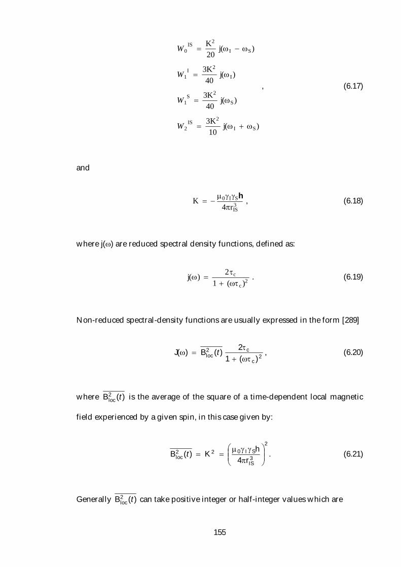
155
W0IS
K2
20j(I S)
W1I
3K2
40j( I)
W1S
3K2
40j(S)
W2IS
3K2
10j( I S)
, (6.17)
and
K
0ISh4rIS
3 , (6.18)
where j() are reduced spectral density functions, defined as:
j()
2c
1 (c )2 . (6.19)
Non-reduced spectral-density functions are usually expressed in the form [289]
2c
c2loc )(1
2)(B)(J
t , (6.20)
where )(B2loc t is the average of the square of a time-dependent local magnetic
field experienced by a given spin, in this case given by:
2
3IS
SI022loc r4
K)(B
ht . (6.21)
Generally )(B2loc t can take positive integer or half-integer values which are

156
equally distributed about zero, such that the average over the entire sample is
zero.
In Eqs. (6.19) and (6.20), c is the correlation time (in seconds); this is
defined as the time constant characterising the decay rate of the correlation
function, G(t) [289]:
)/exp()(B)(G c2loc ttt . (6.22)
The correlation function describes the variation over time of the average of the
square of the local magnetic field, )(B2loc t , and its Fourier transform yields the
spectral density function in Eq. (6.20).
For small molecules in solution, the correlation time is typically very
short, such that the condition 0c << 1 is satisfied. This condition is known as
the fast-motion or extreme-narrowing limit. Conversely, for large molecules in
solution the correlation time is usually much longer and so the condition 0c
>> 1 is satisfied. This limit is referred to as the slow-motion or spin-diffusion
limit. For the results to be presented in this Chapter, only the fast-motion limit
is applicable and so the slow-motion limit will not be considered further here.
In the fast-motion limit, the reduced spectral density function defined in
Eq. (6.19) becomes independent of frequency and is given by
j() = 2c , (6.23)

157
and so the cross-relaxation rate constant becomes
IS K2
2012c 2c
K2c
2
, (6.24)
and hence W0IS and W2
IS are given by
W0IS
K2c
10
W2IS
3K2c
5
. (6.25)
For small molecules in solution, the double-quantum pathway thus makes
the dominant contribution to cross-relaxation, as was stated in Section 6.2.1. The
self-relaxation rate constants are also simplified to:
I = S = K2c , (6.26)
and so, in the fast-motion limit, the cross- and self-relaxation rate constants are
related by
= 2 . (6.27)
Figure 6.3 shows the behaviour of the I- and S-spin magnetizations in a
transient NOE experiment, directly after an inversion pulse has been applied to
the S spins. A homonuclear spin system (spin I = 12) in the fast-motion regime
is assumed and so, using Eq. (6.26), the maximum NOE enhancement in Eq.

158
Figure 6.3. The behaviour of the (a) I-spin and (b) S-spin magnetizations in a transient NOE
experiment during the NOE build-up interval for a pair of homonuclear spin I = 12 nuclei.
Motion in the extreme-narrowing limit has been assumed and = 1.0 s1 and = 0.5 s1.
(6.13) reduces to
max 2
3 3
0.385
. (6.28)
More generally, the maximum transient NOE enhancement in the fast-
motion limit for a pair of spin I = 12 nuclei is given by
max
23 3
S
I
. (6.29)
For an IS spin pair where I = 11B and S = 1H, the maximum NOE

159
enhancement is, by treating 11B as a spin I = 12 nucleus (a valid
approximation, as the quadrupolar interaction renders the satellite transitions
virtually unobservable in an MAS experiment), 1.20.
Figure 6.3a shows that the I-spin signal intensity increases until = max,
at which point the maximum NOE enhancement for a homonuclear spin pair of
0.385 is achieved, before I-spin self-relaxation then returns it to its equilibrium
value. The curve shown in Fig. 6.3a is referred to as an "NOE build-up" curve.
The recovery of the S-spin magnetization to its equilibrium value after the
inversion pulse has been applied is shown in Fig. 6.3b.
6.3 NOEs to Quadrupolar Nuclei
As described in Section 6.1, NOEs to quadrupolar nuclei are rarely
observed as a consequence of the quadrupolar contribution being by far the
most dominant one to spin-lattice relaxation. This can be illustrated by
considering the NOE build-up curves when cross-relaxation is achieved via just
a dipolar mechanism, and when both dipolar and quadrupolar mechanisms are
operative.
NOE build-up curves may be obtained by calculating the Redfield
relaxation matrix [290]. This calculation may be illustrated with the simple case
of a homonuclear spin I = 12 pair. The equation of motion describing such a
system is given by [290]:

160
44
33
22
11
44
33
22
11
4444443344224411
3344333333223311
2244223322222211
1144113311221111
44
33
22
11
R
RRRRRRRRRRRRRRRR
dd
, (6.30)
where R is the relaxation matrix and Rabcd (1 ≤ a, b, c, d ≤ 4) the corresponding
matrix elements. The vector elements 11, 22, 33 and 44 correspond to the
relative populations of the four Zeeman states with mI, mS = +12, +12; 12,
+12; +12, 12 and 12, 12; labelled 1, 2, 3 and 4, respectively. The off-
diagonal relaxation matrix elements may be calculated using the equation
2
2ISISacabcd bVdcVa)(J2R
q
qq , (6.31)
where the spectral density function J(ac) is defined according to:
2
cac
c2
ac 12
20K3)(J , (6.32)
and where the frequencies ac take the values (for a homonuclear spin pair) 0
(for 23); 0 (for 12, 13, 24 and 34) and 20 (for 14) and where the relation
ac = ca is satisfied. The summation of the elements in each row and column
of the relaxation matrix is zero and so the diagonal elements can be obtained
through knowledge of the off-diagonal elements. qISV are tensors and cVa IS
q

161
and bVd ISq their corresponding matrix elements; these tensors are defined
according to
SI2
IS
SISI1IS
SISISI21
0IS
IIV
IIIIV
IIIIII461V
zz
zz
, (6.33)
in terms of the Cartesian operators, Iz and the raising and lowering operators I+
and I, respectively:
Ix 12
I I
Iy i2
I I . (6.34)
The relaxation matrix R is thus:
)2(J2)(J2
)(J2
)(J)2(J22
)(J3
)0(J)(J3
)0(J2
)(J2
)(J3
)0(J3
)0(J)(J2
)(J)2(J2
2)(J
2)(J)2(J2)(J
. (6.35)
The matrix now needs to be transformed into a suitable basis set. For a pair of
spin I = 12 nuclei, products of Cartesian spin angular momentum operators
(so-called "product operators" [76], referred to in Section 2.5 of Chapter 2) are
particularly useful. In this case, the 4 operators E, Iz, Sz and 2IzSz are required,

162
where E is the unity operator. A transformation matrix, U, is then formed
where each row is derived from the diagonal elements of the 4 basis operators
(note that E, Iz and Sz have to be multiplied by E to yield the required 4 4
matrices):
111111111111
1111
21U , (6.36)
and a new relaxation matrix R’ in the Zeeman order basis set is now obtained
by multiplying R by U and its transpose UT (where U = UT):
)(J20000)2(J2)(J
3)0(J)2(J2
3)0(J0
0)2(J23
)0(J)2(J2)(J3
)0(J00000
URUR T
. (6.37)
The equation of motion is now modified to:
0
0
0
0
SI2)(SI2S)(SI)(IE)(E
R
)(SI2)(S)(I)(E
dd
zzzz
zz
zz
zz
z
z , (6.38)
where the expectation values of these operators have the same meaning as
those in Eq. (6.1).

163
Equation (6.38) can be easily solved to yield expressions for the
expectation values of the operators Iz and Sz:
c)2(J2)(J3
)0(JS)(S
)2(J23
)0(JI)(I)(S
c)2(J23
)0(JS)(S
)2(J2)(J3
)0(JI)(I)(I
0
0
0
0
zz
zzz
zz
zzz
, (6.39)
where c is a constant of integration. If the boundary conditions given in Eq. (6.3)
are assumed (i.e., the initial rate limit), then the expressions in Eq. (6.39) are
identical to those in Eqs. (6.5) and (6.6).
For the case of a spin I = 32, spin I = 12 pair the relaxation matrix was
constructed using a basis set consisting of the products of 2 spherical tensor
operators (T0,0 and T1,0) for the spin I = 12 nucleus (spin S) and 4 spherical
tensor operators (T0,0, T1,0, T2,0 and T3,0) for the spin I = 32 nucleus (spin I).
This resulted in 8 operators (T0,0(S)T0,0(I), T0,0(S)T1,0(I), T0,0(S)T2,0(I), T0,0(S)T3,0(I),
T1,0(S)T0,0(I), T1,0(S)T1,0(I), T1,0(S)T2,0(I) and T1,0(S)T3,0(I)) and a relaxation matrix
of dimensions 8 8 was obtained with the aid of the MathNMR Mathematica
program [291]. The matrix was calculated directly in the spherical tensor
operator basis set (i.e., without the need for any transformation as described in
the case of a homonuclear spin I = 12 pair) and, due to the block diagonal
nature of 4 operators in the matrix (i.e., these 4 operators showed correlations

164
only with each other), the equation of motion was modified to one containing a
relaxation matrix of dimensions 4 4. This equation can then easily be solved
with the boundary condition )0(S z = 0S z .
The modified equation of motion describes the time dependence of the
expectation values of the operators T0,0(S)T1,0(I), T0,0(S)T3,0(I), T1,0(S)T0,0(I) and
T1,0(S)T2,0(I). The expectation values of these tensors are defined as T , the
deviation of these tensors from their equilibrium values:
0T)(TT . (6.40)
The evolution of the I-spin magnetization is represented by the operator
T0,0(S)T1,0(I); the magnitude of the expectation value of this operator
(<T0,0(S)T1,0(I)>) is plotted in Fig. 6.4 for the case of an IS spin pair, where I =
11B and S = 1H.
NOE build-up curves are shown in Fig. 6.4 when just dipolar and a
combination of dipolar and quadrupolar mechanisms are present to effect
cross-relaxation. Motion in the extreme-narrowing limit is assumed. In Fig. 6.4a,
the maximum NOE enhancement of 0.43 is achieved when solely dipolar
contributions are incorporated into the calculation of the relaxation matrix
(solid line), whilst the addition of the quadrupolar mechanism with a
quadrupolar coupling parameter, CQ, equal to 0.5 MHz, leads to a significant
reduction of the enhancement to just 0.04 (dashed line). The strong effect of a
quadrupolar coupling is demonstrated further in Fig. 6.4b, where the presence

165
Figure 6.4. NOE build-up curves for an I = 11B, S = 1H spin pair shown for when the
mechanism for cross-relaxation is (a) solely dipolar (solid line) and dipolar and quadrupolar
(dashed line, CQ = 0.5 MHz) in origin and (b) when both dipolar and quadrupolar
contributions are present and CQ = 0.5 MHz (solid line), 1.0 MHz (dashed line) and 1.5 MHz
(dot dashed line). The MathNMR Mathematica program [291] was used for calculating the
curves when a quadrupolar contribution was included. The correlation time c = 100 ps.
of a quadrupolar interaction with CQ = 0.5 MHz (solid line), 1.0 MHz (dotted
line) and 1.5 MHz (dot dashed line) is shown. The increase in CQ continues to
decrease significantly the enhancement to the point where, at CQ = 1.5 MHz,
an enhancement of just 0.006 is expected. The magnitude of this effect, even
when CQ is modest, is thus so great that NOEs to quadrupolar nuclei are
typically too small to be detected.

166
6.4 Transient NOE Enhancement of Borane Adducts
6.4.1 Central Transition 11B{1H} NOE
Transient NOE experiments have been performed on a series of solid
borane adducts, using the pulse sequence shown in Fig. 6.2 under MAS
conditions. This experiment is used instead of the steady-state NOE method
commonly used in the solution state as the long periods of high-power
decoupling needed make it unsuitable for use in solid-state NMR. In each case,
a range of values was used such that an NOE build-up curve like that shown
in Fig. 6.3a was obtained. For each material, the maximum enhancement was
obtained and the value of for which the maximum 11B signal intensity was
seen, max, was determined. In these results, the NOE enhancement is expressed
as a percentage and so is defined as
fI {S}
I(max ) I0
I0 100 , (6.41)
where I(max) and I0 are the I-spin signal intensities at = max and = 0,
respectively. Figure 6.5 shows 1H-decoupled 11B MAS spectra of borane
triphenylphosphine for the cases of = 0 and = max = 650 ms. The 11B
central transition MAS lineshape is broadened by the residual second-order
quadrupolar interaction (the quadrupolar coupling parameter, CQ = 1.2 MHz
and the asymmetry parameter, = 0 [293]) and also shows evidence of 11B-31P J
coupling (J11B-31P = 60 Hz [293]). The increase in signal intensity in Fig. 6.5 is
evidence of a heteronuclear NOE with an NOE enhancement fI{S} = 155%.

167
Figure 6.5. 1H-decoupled 11B MAS spectra of borane triphenylphosphine acquired using the
transient NOE experiment in Fig. 6.2, shown for values of (a) = 0 and (b) = 650 ms. The
experiment was performed at B0 = 9.4 T and the MAS rate was 10 kHz. The chemical shift scale
is referenced to solid BPO4 at 3.3 ppm [292]. The 11B 90° pulse had duration 1.1 s and the 1H
inversion pulse was 2.9 s. The 1H decoupling field strength was ~65 kHz.
When this experiment is performed on the same material in the solution state,
no NOE is observed [287].
The presence of a transient NOE in this material is intriguing given that
11B is a quadrupolar nucleus and that an enhancement is observed only in the
solid state. A likely source of motion on the fast timescale is the rapid rotation
of the BH3 group about its C3 axis that causes a random modulation of the 1H-
11B dipole-dipole interaction. The close proximity of the 11B and 1H nuclei (rIS =
0.117 nm in borane ammonia complex, BH3·NH3 [294]) leads to a strong dipolar

168
interaction and hence a large NOE enhancement. T1 relaxation of quadrupolar
nuclei is often very efficient and usually takes effect more rapidly than any
dipolar-driven cross-relaxation. The presence of an NOE in this material is thus
likely to be due to the absence of a modulation of the 11B quadrupolar
interaction that would lead to efficient quadrupolar relaxation. This arises
because, as the 11B quadrupole tensor is axially symmetric, it is aligned along
the BH3 C3 axis and so rapid reorientation of the BH3 group about this axis
alters very little the 11B quadrupolar interaction. The validity of this rationale is
demonstrated with the absence of a transient 11B{1H} NOE in solid ortho-
carborane, B10H10C2H2. Rapid isotropic tumbling of this cage molecule [295]
causes the modulation of the 1H-11B and 1H-13C dipole-dipole interactions that
is required for NOE enhancement of the 11B and 13C nuclei, respectively.
However, whilst a 13C{1H} NOE enhancement of 63% is observed [287], a
11B{1H} NOE enhancement is not. This is because the isotropic tumbling also
modulates the 11B quadrupolar interaction, so leading to efficient quadrupolar
relaxation and hence no 11B{1H} NOE. The absence of a transient 11B{1H} NOE of
borane triphenylphosphine in the solution state may be similarly explained. In
this case, the rapid tumbling about all Cartesian axes seen in solution
modulates the 11B quadrupolar interaction and destroys the NOE.
Equation (6.29) reveals that a maximum 11B{1H} transient NOE
enhancement of 1.20 would be expected (if 11B is treated as a spin I = 12
nucleus). Expressed as a percentage according to Eq. (6.41), the maximum NOE
enhancement of 120% is less than the 155% observed experimentally in borane
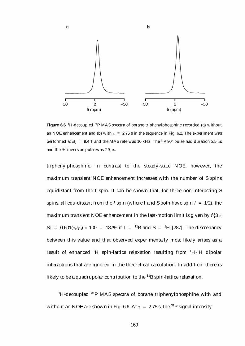
169
Figure 6.6. 1H-decoupled 31P MAS spectra of borane triphenylphosphine recorded (a) without
an NOE enhancement and (b) with = 2.75 s in the sequence in Fig. 6.2. The experiment was
performed at B0 = 9.4 T and the MAS rate was 10 kHz. The 31P 90° pulse had duration 2.5 s
and the 1H inversion pulse was 2.9 s.
triphenylphosphine. In contrast to the steady-state NOE, however, the
maximum transient NOE enhancement increases with the number of S spins
equidistant from the I spin. It can be shown that, for three non-interacting S
spins, all equidistant from the I spin (where I and S both have spin I = 12), the
maximum transient NOE enhancement in the fast-motion limit is given by fI{3
S} = 0.601(IS) 100 = 187% if I = 11B and S = 1H [287]. The discrepancy
between this value and that observed experimentally most likely arises as a
result of enhanced 1H spin-lattice relaxation resulting from 1H-1H dipolar
interactions that are ignored in the theoretical calculation. In addition, there is
likely to be a quadrupolar contribution to the 11B spin-lattice relaxation.
1H-decoupled 31P MAS spectra of borane triphenylphosphine with and
without an NOE are shown in Fig. 6.6. At = 2.75 s, the 31P signal intensity
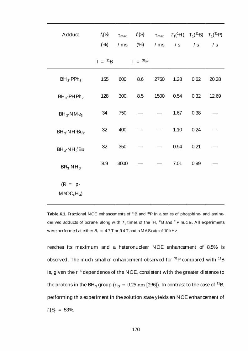
170
Table 6.1. Fractional NOE enhancements of 11B and 31P in a series of phosphine- and amine-
derived adducts of borane, along with T1 times of the 1H, 11B and 31P nuclei. All experiments
were performed at either B0 = 4.7 T or 9.4 T and a MAS rate of 10 kHz.
reaches its maximum and a heteronuclear NOE enhancement of 8.5% is
observed. The much smaller enhancement observed for 31P compared with 11B
is, given the r6 dependence of the NOE, consistent with the greater distance to
the protons in the BH3 group (rIS ≈ 0.25 nm [296]). In contrast to the case of 11B,
performing this experiment in the solution state yields an NOE enhancement of
fI{S} = 53%.
Adduct fI{S}
(%)
I = 11B
max
/ms
fI{S}
(%)
I = 31P
max
/ms
T1(1H)
/s
T1(11B)
/s
T1(31P)
/s
BH3·PPh3
BH3·PHPh2
BH3·NMe3
BH3·NHtBu2
BH3·NH2tBu
BR3·NH3
(R = p-
MeOC6H4)
155
128
34
32
32
8.9
600
300
750
400
350
3000
8.6
8.5
—
—
—
—
2750
1500
—
—
—
—
1.28
0.54
1.67
1.10
0.94
7.01
0.62
0.32
0.38
0.24
0.21
0.99
20.28
12.69
—
—
—
—

171
Transient NOE results for borane triphenylphosphine and a series of other
phosphine- and amine-derived borane adducts are summarised in Table 6.1. T1
relaxation times for 1H, 11B and 31P nuclei are also shown. The 11B{1H} NOE
enhancement of borane diphenylphosphine, BH3·PHPh2, is smaller than that
observed in borane triphenylphosphine. This concurs with the more efficient 1H
and 11B spin-lattice relaxation shown by the T1 values in Table 6.1.
The 11B{1H} NOE enhancements observed for borane trimethylamine,
BH3·NMe3, borane tert-butylamine, BH3·NH2tBu, and borane di-tert-
butylamine, BH3·NHtBu2, are very similar, which is not surprising given the
chemical similarity of these materials. The slightly smaller enhancements
observed with the tert-butylamine and di-tert-butylamine adducts are consistent
with the more efficient 1H and 11B T1 relaxation observed in these solids. The
much smaller enhancement observed for borane tri-para-methoxyphenylamine,
B(p-MeOC6H4)3·NH3, is consistent with the source of the NOE being the more
distant protons attached to the nitrogen atom.
6.4.2 Satellite and Triple-Quantum Transition 11B{1H} NOE
The results shown in the previous section were concerned with the 11B{1H}
NOE enhancement of the 11B central transition. By performing the transient
NOE experiment in Fig. 6.2 over a large spectral width and by modifying the
technique to incorporate triple-quantum filtration, the enhancement of the
satellite and triple-quantum transitions may be obtained, respectively. The

172
Figure 6.7. Pulse sequence and coherence transfer pathway for the transient NOE experiment
that measures the heteronuclear NOE enhancement experienced by the triple-quantum
transition of spin I upon inversion of the populations of the S-spin energy levels. The NOE
build-up interval is denoted .
pulse sequence for the triple-quantum filtered transient NOE experiment is
shown in Fig. 6.7.
1H-decoupled 11B MAS spectra of borane triphenylphosphine recorded
with a spectral width of ~1 MHz are shown in Fig. 6.8, both in the absence of an
NOE (Fig. 6.8a) and with = 550 ms (Fig. 6.8b), when the maximum NOE
enhancement was obtained. The spectra show the expected manifold of
spinning sidebands whose envelope approximately corresponds to the axially
symmetric static satellite-transition lineshape expected for this material. The
maximum NOE enhancement is obtained at = 550 ms (Fig. 6.8b), where an
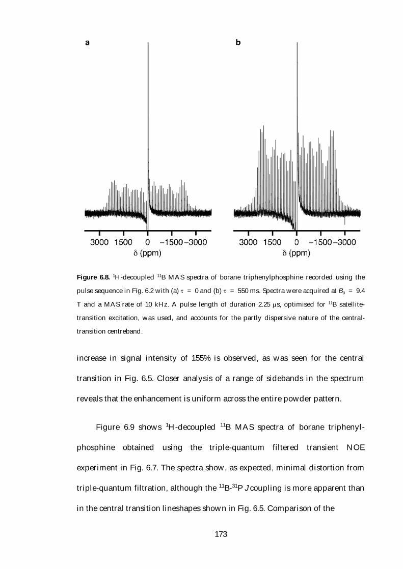
173
Figure 6.8. 1H-decoupled 11B MAS spectra of borane triphenylphosphine recorded using the
pulse sequence in Fig. 6.2 with (a) = 0 and (b) = 550 ms. Spectra were acquired at B0 = 9.4
T and a MAS rate of 10 kHz. A pulse length of duration 2.25 s, optimised for 11B satellite-
transition excitation, was used, and accounts for the partly dispersive nature of the central-
transition centreband.
increase in signal intensity of 155% is observed, as was seen for the central
transition in Fig. 6.5. Closer analysis of a range of sidebands in the spectrum
reveals that the enhancement is uniform across the entire powder pattern.
Figure 6.9 shows 1H-decoupled 11B MAS spectra of borane triphenyl-
phosphine obtained using the triple-quantum filtered transient NOE
experiment in Fig. 6.7. The spectra show, as expected, minimal distortion from
triple-quantum filtration, although the 11B-31P J coupling is more apparent than
in the central transition lineshapes shown in Fig. 6.5. Comparison of the
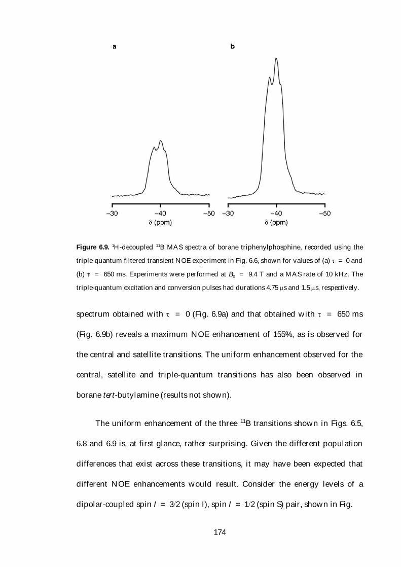
174
Figure 6.9. 1H-decoupled 11B MAS spectra of borane triphenylphosphine, recorded using the
triple-quantum filtered transient NOE experiment in Fig. 6.6, shown for values of (a) = 0 and
(b) = 650 ms. Experiments were performed at B0 = 9.4 T and a MAS rate of 10 kHz. The
triple-quantum excitation and conversion pulses had durations 4.75 s and 1.5 s, respectively.
spectrum obtained with = 0 (Fig. 6.9a) and that obtained with = 650 ms
(Fig. 6.9b) reveals a maximum NOE enhancement of 155%, as is observed for
the central and satellite transitions. The uniform enhancement observed for the
central, satellite and triple-quantum transitions has also been observed in
borane tert-butylamine (results not shown).
The uniform enhancement of the three 11B transitions shown in Figs. 6.5,
6.8 and 6.9 is, at first glance, rather surprising. Given the different population
differences that exist across these transitions, it may have been expected that
different NOE enhancements would result. Consider the energy levels of a
dipolar-coupled spin I = 32 (spin I), spin I = 12 (spin S) pair, shown in Fig.

175
Figure 6.10. Energy level diagram for a dipolar-coupled heteronuclear spin pair consisting of a
spin I = 32 nucleus (I) and a spin I = 12 nucleus (S) shown (a) at thermal equilbrium, (b) after
a 180° pulse has been applied to the S spins and (c) after cross-relaxation via solely the double-
quantum pathway. The energy levels are marked with their relative populations with the
assumption that SI = 3.

176
6.10. In Fig. 6.10a, the energy levels are shown with their relative populations at
thermal equilibrium. By making the approximation that SI = 3 (on the basis
that spin I is 11B and spin S is 1H), the I and S spins have relative population
differences, nI and nS, of 2 and 6, respectively. The relative populations
after an inversion pulse has been applied to the S spins are shown in Fig. 6.10b.
Indicated in Fig. 6.10b, by the rate constant W2IS, are double-quantum pathways
that may be utilised by cross relaxation to return the populations of the energy
levels involved to their equilibrium values. The zero-quantum pathways are not
shown as they make, for small molecules in solution, a minor contribution to
cross-relaxation when there is motion present in the extreme-narrowing limit.
Figure 6.10c shows the energy levels after hypothetical cross-relaxation (solely
via the double-quantum pathway) has acted between the levels indicated in Fig.
6.10b. The population differences across the central, triple-quantum and two
satellite transitions are shown in Fig. 6.10c and reveal that the population
difference across the central transition remains the same at 2, the triple-
quantum transition population difference increases from 6 to 12 and the
difference across the two satellite transitions remain the same at 2 and increase
to 8, respectively.
The perturbations to the populations of the energy levels in an I = 11B, S
= 1H spin pair shown in Fig. 6.10 suggest that an NOE enhancement is
expected for neither the central transition nor one of the satellite transitions,
whilst enhancements of 300% and 100% are expected for the other satellite
transition and the triple-quantum transition, respectively. Whilst the energy
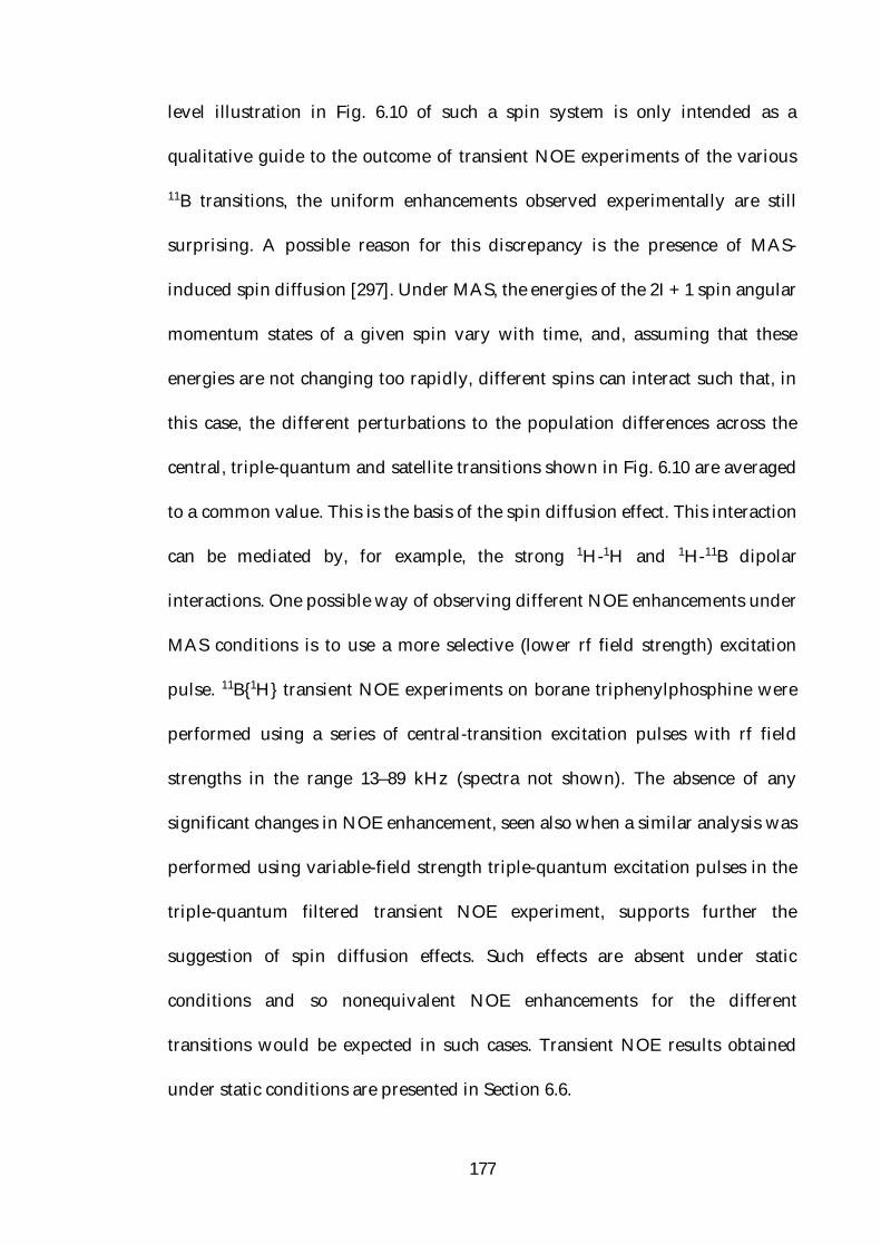
177
level illustration in Fig. 6.10 of such a spin system is only intended as a
qualitative guide to the outcome of transient NOE experiments of the various
11B transitions, the uniform enhancements observed experimentally are still
surprising. A possible reason for this discrepancy is the presence of MAS-
induced spin diffusion [297]. Under MAS, the energies of the 2I + 1 spin angular
momentum states of a given spin vary with time, and, assuming that these
energies are not changing too rapidly, different spins can interact such that, in
this case, the different perturbations to the population differences across the
central, triple-quantum and satellite transitions shown in Fig. 6.10 are averaged
to a common value. This is the basis of the spin diffusion effect. This interaction
can be mediated by, for example, the strong 1H-1H and 1H-11B dipolar
interactions. One possible way of observing different NOE enhancements under
MAS conditions is to use a more selective (lower rf field strength) excitation
pulse. 11B{1H} transient NOE experiments on borane triphenylphosphine were
performed using a series of central-transition excitation pulses with rf field
strengths in the range 13–89 kHz (spectra not shown). The absence of any
significant changes in NOE enhancement, seen also when a similar analysis was
performed using variable-field strength triple-quantum excitation pulses in the
triple-quantum filtered transient NOE experiment, supports further the
suggestion of spin diffusion effects. Such effects are absent under static
conditions and so nonequivalent NOE enhancements for the different
transitions would be expected in such cases. Transient NOE results obtained
under static conditions are presented in Section 6.6.

178
6.5 Variable-Temperature NOE Studies
Variable-temperature 11B{1H} transient NOE experiments were performed
on borane triphenylphosphine. By increasing the temperature, it would be
expected that the correlation time describing the rotation of the BH3 group
about its C3 axis would decrease, so enhancing the efficiency of dipolar-driven
cross-relaxation and increasing the NOE enhancement. Conversely, reducing
the temperature would be expected to increase the correlation time and so
result in a decrease in the enhancement.
Transient NOE enhancements for borane triphenylphoshine over the
temperature range 223–353 K are shown in Fig. 6.11a. At temperatures of 293 K
and above, the enhancement is essentially constant with fI{S} ~155%. Below
room temperature, the enhancement remains constant until 273 K, beyond
which point the enhancement decreases such that, at 223 K, it is substantially
reduced to 94%. The max values obtained from these experiments are shown in
Fig. 6.11b and show a steady decrease as the temperature is reduced.
In the theoretical derivation of the NOE in Sections 6.2.2 and 6.3 the
simplification that the correlation time, c, is in the fast-motion limit (0c << 1)
was made. This typically corresponds to values of c in the range 1012–109 s.
Given that a variation in temperature causes a change of the correlation time
and hence a change of the NOE enhancement, a comparison of the NOE build-
up curves for a range of values of c should enable an estimate of its value to be
made. NOE build-up curves for a range of values of c between 50 ps and 100 ns
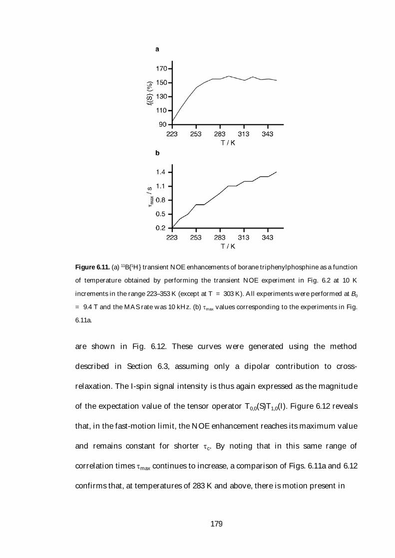
179
Figure 6.11. (a) 11B{1H} transient NOE enhancements of borane triphenylphosphine as a function
of temperature obtained by performing the transient NOE experiment in Fig. 6.2 at 10 K
increments in the range 223–353 K (except at T = 303 K). All experiments were performed at B0
= 9.4 T and the MAS rate was 10 kHz. (b) max values corresponding to the experiments in Fig.
6.11a.
are shown in Fig. 6.12. These curves were generated using the method
described in Section 6.3, assuming only a dipolar contribution to cross-
relaxation. The I-spin signal intensity is thus again expressed as the magnitude
of the expectation value of the tensor operator T0,0(S)T1,0(I). Figure 6.12 reveals
that, in the fast-motion limit, the NOE enhancement reaches its maximum value
and remains constant for shorter c. By noting that in this same range of
correlation times max continues to increase, a comparison of Figs. 6.11a and 6.12
confirms that, at temperatures of 283 K and above, there is motion present in

180
Figure 6.12. NOE build-up curves for an I = 11B, S = 1H spin pair for a range of correlation
times. The 11B nucleus is treated as a spin I = 12 nucleus (CQ = 0). The MathNMR
Mathematica program was again used for calculating these curves. Due to the large number of
curves shown, each one is individually labelled with the correlation time with which it was
obtained.
the extreme-narrowing limit. In addition, the decrease in NOE enhancement
seen at longer correlation times qualitatively matches the trend seen in Fig.
6.11a.
The variation in NOE enhancement shown in Fig. 6.11 may also be
rationalised by considering the I- and S-spin self-relaxation rates. The 1H and
11B T1 relaxation times in borane triphenylphosphine are shown in Fig. 6.13.
Both nuclei show the same trend of decreasing T1 times as temperature is
decreased, although there is a much greater change in the case of the protons.
The enhanced self-relaxation of the 1H and 11B nuclei takes effect progressively
more rapidly than cross-relaxation as the temperature is decreased and so
accounts for the decrease in NOE enhancement shown in Fig. 6.11a.

181
Figure 6.13. 1H (solid line) and 11B (dashed line) T1 relaxation times as a function of temperature
in borane triphenylphosphine.
6.6 NOE Enhancement under Static Conditions
The transient 11B{1H} NOE experiment was performed on borane
triphenylphosphine under non-spinning (static) conditions. The 11B spectrum
of this material is shown in Fig. 6.14, recorded at applied magnetic field
strengths of 4.7 T and 9.4 T. As expected, the spectrum in Fig. 6.14b, obtained at
B0 = 4.7 T, features a second-order quadrupolar broadened central-transition
lineshape with a width of ~100 ppm, twice the 50 ppm width seen in the
spectrum in Fig. 6.14a, recorded at B0 = 9.4 T. Neither of the spectra in Fig. 6.14
appear like the static central-transition lineshape shown in Fig. 3.4a in Chapter
3. This is because the presence of the 11B-31P dipolar coupling ( DPAS ~1 kHz),
combined with the second-order quadrupolar interaction, yields a spectrum
consisting of two overlapping central-transition powder patterns, one narrowed
and the other broadened with respect to the single powder pattern that would
be obtained if only quadrupolar broadening was present. The broader powder
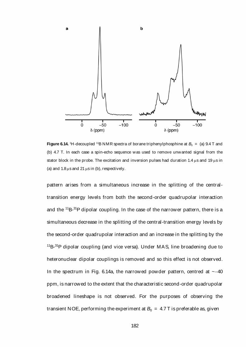
182
Figure 6.14. 1H-decoupled 11B NMR spectra of borane triphenylphosphine at B0 = (a) 9.4 T and
(b) 4.7 T. In each case a spin-echo sequence was used to remove unwanted signal from the
stator block in the probe. The excitation and inversion pulses had duration 1.4 s and 19 s in
(a) and 1.8 s and 21 s in (b), respectively.
pattern arises from a simultaneous increase in the splitting of the central-
transition energy levels from both the second-order quadrupolar interaction
and the 11B-31P dipolar coupling. In the case of the narrower pattern, there is a
simultaneous decrease in the splitting of the central-transition energy levels by
the second-order quadrupolar interaction and an increase in the splitting by the
11B-31P dipolar coupling (and vice versa). Under MAS, line broadening due to
heteronuclear dipolar couplings is removed and so this effect is not observed.
In the spectrum in Fig. 6.14a, the narrowed powder pattern, centred at ~40
ppm, is narrowed to the extent that the characteristic second-order quadrupolar
broadened lineshape is not observed. For the purposes of observing the
transient NOE, performing the experiment at B0 = 4.7 T is preferable as, given

183
Figure 6.15. 1H-decoupled 11B NMR spectra of borane triphenylphosphine, recorded using the
transient NOE experiment in Fig. 6.2 at B0 = 4.7 T with (a) = 0 and (b) = 700 ms. The
numbers indicated correspond to the maximum transient NOE enhancements observed at these
points of the powder pattern.
the greater breadth of the spectrum at this magnetic field strength, it enables the
enhancement across the powder pattern to be more closely analysed.
11B NMR spectra of borane triphenylphosphine recorded using the
transient NOE experiment are shown in Fig. 6.15. In Fig. 6.15a the spectrum
obtained without an NOE is shown, whilst the spectrum recorded with = 700
ms is shown in Fig. 6.15b. The maximum signal intensity is obtained across the
entire powder pattern at this value of and, clearly, a non-uniform
enhancement is observed. The enhancements observed at the extremities of
each of the two overlapping powder patterns are indicated in Fig. 6.15b and
vary strongly in the range fI{S} = 67–175%, compared with the uniform

184
Figure 6.16. 1H-decoupled 11B NMR spectra of borane di-tert-butylamine recorded at B0 = 4.7 T
using the transient NOE experiment in Fig. 6.2 with (a) = 0 and (b) = 300 ms. The numbers
indicated correspond to the maximum transient NOE enhancements observed at these points of
the powder pattern.
enhancement of 155% observed under MAS conditions. The NOE build-up
curves seen for these four features of the lineshape (not shown) reveal,
unsurprisingly, that the signal intensity increases at a greater rate the larger the
enhancement.
This variation in transient NOE enhancement under static conditions is
also seen in the 11B NMR spectrum of borane di-tert-butylamine, shown in Fig.
6.16. The lower gyromagnetic ratios of 14N and 15N compared to 31P, and the
low natural abundance of 15N (0.37%), means that the significant dipolar
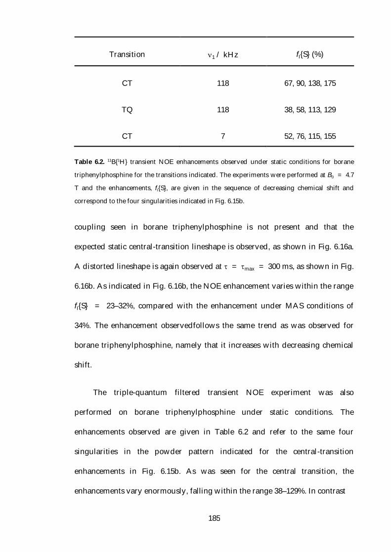
185
Table 6.2. 11B{1H} transient NOE enhancements observed under static conditions for borane
triphenylphosphine for the transitions indicated. The experiments were performed at B0 = 4.7
T and the enhancements, fI{S}, are given in the sequence of decreasing chemical shift and
correspond to the four singularities indicated in Fig. 6.15b.
coupling seen in borane triphenylphosphine is not present and that the
expected static central-transition lineshape is observed, as shown in Fig. 6.16a.
A distorted lineshape is again observed at = max = 300 ms, as shown in Fig.
6.16b. As indicated in Fig. 6.16b, the NOE enhancement varies within the range
fI{S} = 23–32%, compared with the enhancement under MAS conditions of
34%. The enhancement observedfollows the same trend as was observed for
borane triphenylphosphine, namely that it increases with decreasing chemical
shift.
The triple-quantum filtered transient NOE experiment was also
performed on borane triphenylphosphine under static conditions. The
enhancements observed are given in Table 6.2 and refer to the same four
singularities in the powder pattern indicated for the central-transition
enhancements in Fig. 6.15b. As was seen for the central transition, the
enhancements vary enormously, falling within the range 38–129%. In contrast
Transition 1 / kHz fI{S} (%)
CT
TQ
CT
118
118
7
67, 90, 138, 175
38, 58, 113, 129
52, 76, 115, 155
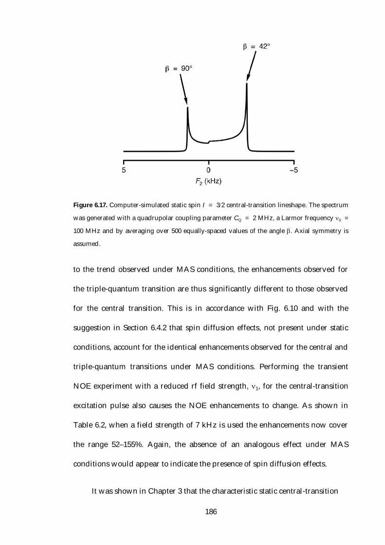
186
Figure 6.17. Computer-simulated static spin I = 32 central-transition lineshape. The spectrum
was generated with a quadrupolar coupling parameter CQ = 2 MHz, a Larmor frequency 0 =
100 MHz and by averaging over 500 equally-spaced values of the angle . Axial symmetry is
assumed.
to the trend observed under MAS conditions, the enhancements observed for
the triple-quantum transition are thus significantly different to those observed
for the central transition. This is in accordance with Fig. 6.10 and with the
suggestion in Section 6.4.2 that spin diffusion effects, not present under static
conditions, account for the identical enhancements observed for the central and
triple-quantum transitions under MAS conditions. Performing the transient
NOE experiment with a reduced rf field strength, 1, for the central-transition
excitation pulse also causes the NOE enhancements to change. As shown in
Table 6.2, when a field strength of 7 kHz is used the enhancements now cover
the range 52–155%. Again, the absence of an analogous effect under MAS
conditions would appear to indicate the presence of spin diffusion effects.
It was shown in Chapter 3 that the characteristic static central-transition

187
lineshape arises as a consequence of the different perturbation experienced by
each crystallite as a result of the second-order quadrupolar interaction. The
powder pattern observed is thus the result of a summation of a range of
frequencies that depend on the angles , and , as described by Eq. (3.23) in
Chapter 3. In Fig. 6.17 the static spin I = 32 central-transition lineshape is
shown, annotated with values of the angle (one of the Euler angles defined in
Section 3.3.1) that give rise to the largest and smallest resonance frequencies.
The greatest positive second-order perturbation to the central-transition
frequency is observed when = 90°, whilst the largest negative second-order
perturbation is observed when = 42°. The presence of an NOE enhancement
that varies across the powder pattern is thus an indication that the NOE is
dependent on crystallite orientation. This is considered using theoretical
arguments in the next section.
6.7 Theoretical Studies of Relaxation
In attempting to rationalise the NOE enhancements shown in the previous
section, an obvious comparison to be made is the T1 relaxation behaviour under
static and MAS conditions. The anisotropy of spin-lattice relaxation is well-
known, with one of the first reported examples being the orientational
dependence of 13C spin-lattice relaxation in powdered benzene under static
conditions [298]. The presence of enhanced spin diffusion effects under MAS
conditions has been used to demonstrate the observation of a common T1 value
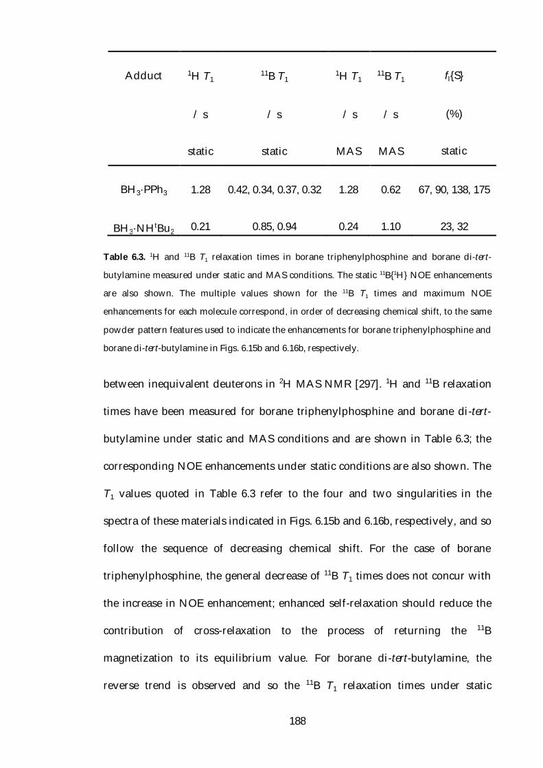
188
Table 6.3. 1H and 11B T1 relaxation times in borane triphenylphosphine and borane di-tert-
butylamine measured under static and MAS conditions. The static 11B{1H} NOE enhancements
are also shown. The multiple values shown for the 11B T1 times and maximum NOE
enhancements for each molecule correspond, in order of decreasing chemical shift, to the same
powder pattern features used to indicate the enhancements for borane triphenylphosphine and
borane di-tert-butylamine in Figs. 6.15b and 6.16b, respectively.
between inequivalent deuterons in 2H MAS NMR [297]. 1H and 11B relaxation
times have been measured for borane triphenylphosphine and borane di-tert-
butylamine under static and MAS conditions and are shown in Table 6.3; the
corresponding NOE enhancements under static conditions are also shown. The
T1 values quoted in Table 6.3 refer to the four and two singularities in the
spectra of these materials indicated in Figs. 6.15b and 6.16b, respectively, and so
follow the sequence of decreasing chemical shift. For the case of borane
triphenylphosphine, the general decrease of 11B T1 times does not concur with
the increase in NOE enhancement; enhanced self-relaxation should reduce the
contribution of cross-relaxation to the process of returning the 11B
magnetization to its equilibrium value. For borane di-tert-butylamine, the
reverse trend is observed and so the 11B T1 relaxation times under static
Adduct 1H T1
/ s
static
11B T1
/ s
static
1H T1
/ s
MAS
11B T1
/ s
MAS
fI{S}
(%)
static
BH3·PPh3
BH3·NHtBu2
1.28
0.21
0.42, 0.34, 0.37, 0.32
0.85, 0.94
1.28
0.24
0.62
1.10
67, 90, 138, 175
23, 32
189
conditions are consistent with the NOE enhancements. For both materials, very
little change is seen in the 1H T1 relaxation times measured under static
conditions compared with those under MAS. Whilst T1 relaxation clearly has a
role to play in the observed NOE enhancements, the trends observed under
static conditions may not be explained by a consideration solely of the T1 values
given in Table 6.3.
To rationalise the static NOE enhancements, a consideration of all the
sources of relaxation is needed. To do this, the Hamiltonian describing the
dipolar interaction between two non-equivalent spins I and S, Hdd, is required.
A convenient formalism with which to express this Hamiltonian is the spherical
tensor form, where an interaction B is described by a Hamiltonian, HB:
H B (1)pA l ,p
B
l0
2
pl
l Tl , p
B , (6.42)
where A l ,pB and Tl , p
B are referred to as the spatial and spin tensor components of
the Hamiltonian, respectively. The latter are identical to the spherical tensor
operators, Tl,p, introduced in Chapter 2. For the dipolar interaction, the only
non-zero component of the tensor A l ,pB is, when expressed in the PAS of the
dipolar coupling tensor, PAS0,2A . Terms with l = 0 and ±1 are zero as a
consequence of the dipolar coupling tensor being (like the electric field gradient
tensor) traceless. Components of the spatial tensor with p = ±1 and ±2 are
neglected as a consequence of the "high-field" approximation being made. In
this approximation, the Zeeman interaction is assumed to be dominant and

190
only those terms which commute with the Zeeman Hamiltonian are considered;
these terms are described as "secular". The component PAS0,2A is given by:
PASD
PAS0,2 6A , (6.43)
where DPAS is the dipolar coupling parameter in the PAS of the dipolar
coupling tensor and is defined as in Eq. (2.50) in Chapter 2. Given the
simplification described in Eq. (6.43), the first-order average Hamiltonian in the
laboratory frame, Hdd, is thus
H dd A2,0PAST2 ,0
6DPAS T2,0
. (6.44)
Equation (6.44) is only sufficient for describing the dipolar interaction
experienced by the range of crystallite orientations in a powder if the IS
internuclear vector is coincident with the laboratory frame z axis, i.e., if the
dipolar coupling PAS and laboratory frames are coincident. Generally, this
condition does not hold for the majority of crystallites and so the following
transformation is required, where , and are Euler angles relating the PAS
and laboratory frames of reference and D m , m2 (, , ) are Wigner rotation
matrix elements:
2
2
PAS,2
2,
Lab,2 A),,(DA
mmmmm , (6.45)
and if only secular components of the dipolar coupling tensor in the high-field

191
approximation (i.e., m’ = m = 0) are used, this reduces to
PAS0,2
20,0
Lab0,2 A),,(DA . (6.46)
Equation (6.44) thus becomes:
H dd 6 D
PAS
2(3 cos2 1)T2 ,0 . (6.47)
Given that the tensor operator T2,0 may also be expressed in the form
T2 ,0
16
(3IzSz I S) , (6.48)
Eq. (6.47) is thus identical to the Hamiltonian in Eq. (2.48) in Chapter 2, where
the former is expressed in spherical tensor operators and the latter in terms of
Cartesian operators.
The neglect of second-rank components of the spatial tensor with m, m’ ≠
0 leads to the Hamiltonians in Eqs. (6.47) and, in Chapter 2, Eq. (2.48) being
referred to as "truncated" or secular. In an attempt to rationalise the static NOE
results in the previous section, these terms (i.e., those that do not commute with
the Zeeman Hamiltonian and that are termed "non-secular") need to be
considered. To do this, two rotations are needed to obtain the components of
the dipolar coupling tensor in the laboratory frame, A2, mLab , in terms of those
defined in the dipolar coupling PAS, A2, mPAS . To perform this transformation, an
intermediate frame of reference is used and is referred to as the molecular

192
Figure 6.18. Illustration of the angles and that relate the dipolar coupling PAS, molecular
and laboratory frames of reference (shown for the case of a borane phosphine adduct). The
angle (not shown) is the azimuthal angle that the 1H nuclei subtend as they rotate about the
BH3 C3 axis in the cone indicated.
frame. The three frames of reference are shown in Fig. 6.18, where the
molecular frame is defined such that its z axis is coincident with (in the case of
borane triphenylphosphine) the BP axis, i.e., it is aligned along the BH3 C3 axis.
The rotation from the PAS of the 1H-11B dipolar coupling tensor to the
molecular frame is defined using the angles and , where is the (polar) angle
between the BH internuclear vector and the BH3 C3 axis and is the
corresponding azimuthal angle. The transformation from the molecular frame
to the laboratory frame is described solely by the angle , which is defined as
the angle between the BP bond and the static magnetic field (i.e., the laboratory
frame z axis). Given the reference frames shown in Figure 6.18, Eq. (6.46) thus
becomes
A2, m
Lab D m ,n2 (0, , )Dn , m
2 (0, , 0)A2, m PAS
m 2
2
n 2
2 , (6.49)

193
and by remembering that in its PAS the dipolar coupling tensor has non-zero
components only when m = 0, this reduces to
A2, m
Lab D0 ,n2 (0, , )Dn , m
2 (0, , 0)A2,0PAS
n 2
2 . (6.50)
The angle in Fig. 6.18 is analogous to the angle used with the other
Euler angles and to describe the transformation of the quadrupole tensor
from its PAS to the laboratory frame in Chapter 3 and that is used in Fig. 6.17 to
indicate the extremities of the static central-transition lineshape. Consequently,
evaluation of Eq. (6.50) enables the modulation of the 1H-11B dipolar interaction
for a range of crystallite orientations to be considered, so providing a possible
rationale for the results in the previous section.
Evaluation of Eq. (6.50) with m = 0, ±1 and ±2 yields the following
expressions for A2,0Lab , A2,1
Lab and A2,2Lab :
A2,0Lab 6Q
PAS 34
sin 2 sin 2 cos 2
14
3 cos2 1 3 cos2 1
3 sin cos sin cos cos
, (6.51)

194
A2,1Lab 6Q
PAS exp 2i 332
sin 2 sin 1 cos
m exp i 38
sin cos sin 1 m 2 cos 1 cos
m 38
3 cos2 1 sin cos
m exp i 38
sin cos sin 1 2 cos 1 m cos
exp 2i 332
sin 2 sin 1 m cos
, (6.52)
and
A2,2Lab 6Q
PAS exp 2i 38
sin 2 cos4 2
m exp i 38
sin cos sin 1 cos
3
323 cos2 1 sin 2
exp i 38
sin cos sin 1 m cos
exp m2i 38
sin 2 sin 4 2
. (6.53)
The inclusion of components of the dipolar coupling tensor with non-zero
coherence order means that the Hamiltonian describing the interaction between
spins I and S, H ddLab , is given by:
H ddLab A2 ,0
LabT2,0 A2 ,1Lab T2,1 A2 ,1
LabT2 ,1 A2,2Lab T2 ,2 A2,2
LabT2 ,2 . (6.54)
195
The physical interpretation of Eq. (6.54) and its meaning in the context of
relaxation may be shown by considering the evolution of the density operator,
(t), under a Hamiltonian, H. This may be accomplished by using the Liouville-
von Neumann equation, introduced in Chapter 2:
d(t )
d t i H , (t) . (6.55)
The Hamiltonian is commonly expressed as the sum of a static part, H0, and a
random time-dependent part, H1(t). For the case of two dipolar-coupled spins I
and S, H0 and H1(t) are thus defined as:
H 0 0Iz 0Sz
H1(t) HddLab (t )
. (6.56)
The time dependence of H ddLab (t ), whilst not stated in Eq. (6.54), is
obviously the result of the rotation of the BH3 group about its C3 axis with a
correlation time of 2c seconds such that the 1H nuclei subtend the azimuthal
angle = 2tc degrees. This is analogous to the definition of the angle Rt in
Chapter 3 that was used for determining the effect of sample rotation on the
second-order quadrupolar perturbation of the energy levels of half-integer
quadrupolar nuclei.
To consider the effect of an interaction such as dipolar coupling,
perturbation theory is often used. In an analogous manner to the quadrupolar
interaction in Chapter 3, the dipolar interaction is treated as a perturbation of

196
the dominant Zeeman Hamiltonian. A transformed density operator, T(t), and
a transformed time-dependent Hamiltonian, H1T (t), are defined as
T (t) exp iH 0t t exp iH 0t H1
T (t) exp iH 0t H1 t exp iH 0t , (6.57)
in which case the equation of motion of T(t) is
dT (t )
d t i H1
T t , T (t ) . (6.58)
In this transformed representation, known as the interaction
representation, (t) evolves under solely the action of the random Hamiltonian
H1T t ; evolution under the much larger static Hamiltonian, H0(t), is factored
out.
The spherical tensor operators in Eq. (6.54), which make up the spin part
of the dipolar Hamiltonian, may also be expressed in terms of Cartesian
operators:
T2,0 16
3IzSz I S
23
IzSz 14
IS IS
T2 ,1 m 12
ISz IzS
T2 ,2 12
IS
, (6.59)

197
where the definitions of the operators Ix and Iy in terms of the raising and
lowering operators I+ and I have been used:
Ix 12
I I
Iy i2
I I . (6.60)
The Cartesian operators in Eq. (6.59) evolve under the static Hamiltonian at
characteristic frequencies, C; this is described by the equation
exp iH 0t C exp iH 0t exp iCt C , (6.61)
for the general case of an operator C. The characteristic frequencies for the
operators given in Eq. (6.59) are shown in Table 6.4, where the former are
labelled Cdd and the latter Cdd. Oscillations at the Larmor frequencies of the I
and S spins, I and S, respectively, lead to spin-lattice relaxation of the I and S
spins and so correspond to the W1I and W1
S pathways indicated in Fig. 6.1b. The
I+Sz and ISz terms thus lead to relaxation via the former pathway and the IzS+
and IzS terms relaxation via the latter. Table 6.4 shows that the terms I+S and
IS+ lead to oscillations at frequencies of I + S and I S, respectively, and
so these terms are responsible for the zero-quantum cross-relaxation pathway
indicated W0IS in Fig. 6.1b. Finally, cross-relaxation via the double-quantum
pathway W2IS arises by oscillation at frequencies of (I + S) and (I + S) and
so is due to the presence the terms IS and I+S+, respectively. The implications
of these characteristic frequencies is that the T2,±1 tensor operators form the spin

198
Table 6.4. Characteristic frequencies at which the operators comprising the dipolar
Hamiltonian, Cdd, evolve at under the effects of H0.
part of the Hamiltonian that is responsible for I- and S-spin T1 relaxation, whilst
the T2,0 and T2,±2 operators form the spin components of the parts of the
Hamiltonian responsible for zero- and double-quantum cross-relaxation,
respectively. Analysis of the corresponding spatial components of the
Hamiltonian, A2,0Lab , A2,1
Lab and A2,2Lab , will thus enable the orientational
dependence of these relaxation processes to be determined and so enable the
static 11B{1H} NOE results to be explained. Equations (6.51–6.53) reveal that
Cdd Cdd
IzSz
I+S
IS+
I+Sz
ISz
IzS+
IzS
I+S+
IS
0
I + S
I S
I
I
S
S
(I + S)
(I + S)

199
Figure 6.19. Amplitude of the real part of the component indicated with increasing , shown for
values of = 42° (solid line) and 90° (dashed line). The angle is fixed at 70.5°.
these tensors are complex functions. In the subsequent discussion, only the real
components of each will be considered.
The amplitude of the component A2,1Lab as is incremented (i.e., as the BH3
group rotates) is shown in Fig. 6.19, for values of = 42° and 90°. As described
in Section 6.6, these values of the Euler angle yield the greatest negative and
positive second-order quadrupolar perturbations to the central-transition
frequency, respectively. It is clear that, over the course of a rotation, this
component experiences a much greater modulation when = 90° than when
= 42°. Given that this component comprises the part of the Hamiltonian
responsible for I (and S) spin T1 relaxation, Fig. 6.19 indicates that, by virtue of
the greater modulation of this function when = 90°, 11B T1 relaxation is more
efficient at this crystallite orientation. More efficient T1 relaxation reduces the
NOE and hence, this observation concurs with the experimental results in Figs.
6.15 and 6.16.
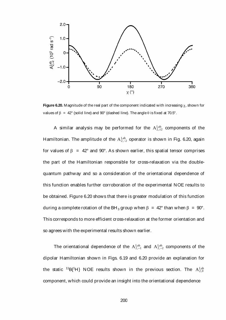
200
Figure 6.20. Magnitude of the real part of the component indicated with increasing , shown for
values of = 42° (solid line) and 90° (dashed line). The angle is fixed at 70.5°.
A similar analysis may be performed for the A2,2Lab components of the
Hamiltonian. The amplitude of the A2,2Lab operator is shown in Fig. 6.20, again
for values of = 42° and 90°. As shown earlier, this spatial tensor comprises
the part of the Hamiltonian responsible for cross-relaxation via the double-
quantum pathway and so a consideration of the orientational dependence of
this function enables further corroboration of the experimental NOE results to
be obtained. Figure 6.20 shows that there is greater modulation of this function
during a complete rotation of the BH3 group when = 42° than when = 90°.
This corresponds to more efficient cross-relaxation at the former orientation and
so agrees with the experimental results shown earlier.
The orientational dependence of the A2,1Lab and A2,2
Lab components of the
dipolar Hamiltonian shown in Figs. 6.19 and 6.20 provide an explanation for
the static 11B{1H} NOE results shown in the previous section. The A2,0Lab
component, which could provide an insight into the orientational dependence

201
Figure 6.21. Amplitude of the real part of the component indicated when m = 1 (solid line)
and 2 (dashed line) as a function of the angle .
of cross-relaxation via the zero-quantum pathway, is not considered here as this
pathway makes (for small molecules in solution) only a minor contribution to
the NOE in the fast-motion limit.
A more complete consideration of the modulation of the A2,1Lab and A2,2
Lab
components over the range of orientations present in a powdered solid is
shown in Fig. 6.21. The modulation of each component is defined as
A2 , mLab A2 , m
Lab max A2 , m
Lab min , (6.62)
where A2 , mLab max
and A2 , mLab min
are the maximum and minimum values of these
functions for 0 ≤ ≤ 360°. Figure 6.21 reveals that the modulation of these
functions repeat every 90° for the A2,1Lab component and every 180° for the A2,2
Lab
component. Maximum and minimum values are reached in the former case at
202
= 0° and 90° and at = 45° and 135°, respectively. Likewise, for the A2,2Lab
components, maxima and minima are seen at = 18° and 162° and at = 90°,
respectively.
6.8 Conclusions
The presence of 11B{1H} NOEs in a range of borane adducts have been
shown. NOEs in the solid state are rare and NOEs to quadrupolar nuclei are
even more scarce; their observation here is due to the rapid rotation of the BH3
group about its C3 axis that modulates very little the 11B quadrupolar
interaction. 31P{1H} NOEs in a series of phosphine-derived borane adducts have
confirmed the protons attached to the boron atom to be the source of the NOE;
the resultant enhancements in these and a range of amine-derived adducts have
been rationalised in terms of the measured 1H, 11B and 31P T1 relaxation times.
11B{1H} central-transition, satellite-transition and triple-quantum transition
NOE enhancements have been measured and been shown to be equivalent
under MAS conditions. This unexpected result has been rationalised as being
due to MAS-enhanced spin diffusion effects. The observation of an NOE to a
quadrupolar nucleus in the solid state is a very interesting one, especially given
its absence in the solution state. Whilst it may be that such an observation is
limited to this particular group of materials, the presence of an NOE
enhancement does, nevertheless, indicate that the nuclear Overhauser effect
may be a useful source of insight into the dynamics of quadrupolar nuclei in the

203
solid state.
Variable-temperature 11B{1H} transient NOE experiments have revealed a
reduction in signal enhancement with decreasing temperature. Such an
observation has been shown to be consistent with an increased correlation time
and more efficient 1H and 11B T1 relaxation at lower temperatures.
Transient NOE experiments performed under static conditions have
revealed a variable enhancement across the powder pattern. In addition,
different central-transition and triple-quantum enhancements have been
observed. Calculations of the orientational dependence of the spatial tensor
components of the dipolar Hamiltonian with coherence order ±1 and ±2 have
been used to explain this behaviour. A consideration of the former has shown
there to be more efficient T1 relaxation when the angle = 90°, whilst analysis
of the latter has demonstrated cross-relaxation to be more efficient when =
42°. Both of these observations concur with the trends observed experimentally.
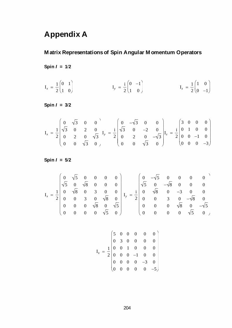
204
Appendix A
Matrix Representations of Spin Angular Momentum Operators
Spin I = 12
Ix
12
0 11 0
Iy
i2
0 11 0
Iz
12
1 00 1
Spin I = 32
Ix 12
0 3 0 03 0 2 0
0 2 0 30 0 3 0
Iy i2
0 3 0 03 0 2 0
0 2 0 30 0 3 0
Iz i2
3 0 0 00 1 0 00 0 1 00 0 0 3
Spin I = 52
Ix 12
0 5 0 0 0 05 0 8 0 0 0
0 8 0 3 0 00 0 3 0 8 00 0 0 8 0 50 0 0 0 5 0
Iy i2
0 5 0 0 0 05 0 8 0 0 0
0 8 0 3 0 00 0 3 0 8 00 0 0 8 0 50 0 0 0 5 0
Iz 12
5 0 0 0 0 00 3 0 0 0 00 0 1 0 0 00 0 0 1 0 00 0 0 0 3 00 0 0 0 0 5

205
Appendix B
Matrix Representations of Spherical Tensor Operators, Tl,p
This appendix contains matrix representations of spherical tensor
operators of spin I = 12, spin I = 1 and spin I = 32 nuclei. Only second-rank
operators are shown for spin I = 32 nuclei, the remaining operators may be
found in Ref. [76].
Spin I = 12
T0 ,0
12
1 00 1
T1,1
0 01 0
T1,0
12
1 00 1
T1,1
0 10 0
Spin I = 1
T0 ,0 13
1 0 00 1 00 0 1
T1,0 12
1 0 00 0 00 0 1
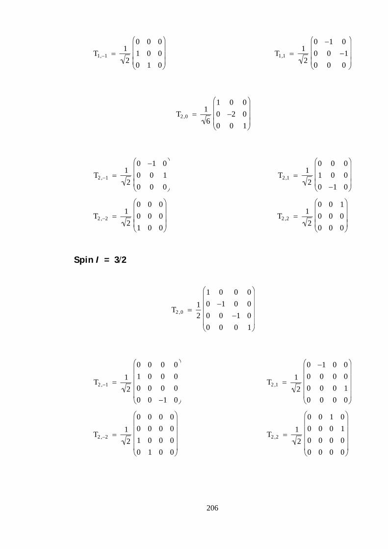
206
T1,1 12
0 0 01 0 00 1 0
T1,1 12
0 1 00 0 10 0 0
T2 ,0 16
1 0 00 2 00 0 1
T2 ,1 12
0 1 00 0 10 0 0
T2 ,2 12
0 0 00 0 01 0 0
T2,1 12
0 0 01 0 00 1 0
T2 ,2 12
0 0 10 0 00 0 0
Spin I = 32
T2 ,0 12
1 0 0 00 1 0 00 0 1 00 0 0 1
T2 ,1 12
0 0 0 01 0 0 00 0 0 00 0 1 0
T2 ,2 12
0 0 0 00 0 0 01 0 0 00 1 0 0
T2 ,1 12
0 1 0 00 0 0 00 0 0 10 0 0 0
T2 ,2 12
0 0 1 00 0 0 10 0 0 00 0 0 0

207
Appendix C
Reduced Rotation Matrix Elements, d p ,pl ()
This appendix lists single-, second- and fourth-rank reduced rotation
matrix elements. Only fourth-rank elements relevant to calculations in Chapter
3 are shown.
l = 1
d1,11 d 1,1
1 12
(1 cos )
d1,11 d 1,1
1 12
(1 cos )
d1,01 d 1,0
1 d 0 ,11 d 0 ,1
1 12
sin
d 001 cos
l = 2
d 2,22 d 2,2
2 14
(1 cos )2
d 2,22 d 2 ,2
2 14
(1 cos )2
d 2,12 d 2 ,1
2 d1,22 d 1,2
2 12
sin (1 cos )
d 2,12 d 2,1
2 d 1,22 d1,2
2 12
sin (1 cos )
d 2,02 d 2,0
2 d 0,22 d 0,2
2 38
(sin 2 )
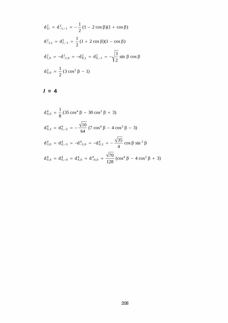
208
d112 d 1,1
2 12
(1 2 cos )(1 cos )
d 1,12 d1,1
2 12
(1 2 cos )(1 cos )
d1,02 d 1,0
2 d 0,12 d 0 ,1
2 32
sin cos
d 0,02
12
(3 cos2 1)
l = 4
d 0,04
18
(35 cos4 30 cos2 3)
d 0,24 d 0 ,2
4 10
64(7 cos4 4 cos2 3)
d 3,04 d 0 ,3
4 d 3,04 d 0,3
4 354
cos sin 3
d 0,44 d 0 ,4
4 d 4,04 d 4 ,0
4 70
128(cos4 4 cos2 3)

209
Appendix D
Coefficients, c l , l
p (), Quantifying the Evolution of Spherical
Tensor Operators under a First-Order Quadrupolar Splitting
Spin I = 1
c1,11 () c1,1
1 () c2,21 () c2 ,2
1 () cos Q
c2,11 () c1,2
1 () c2 ,11 () c1,2
1 () i sin Q
Spin I = 32
c1,11 () c1,1
1 () 15
(2 3 cos 2Q )
c2 ,11 () c1,2
1 () c2 ,11 () c1,2
1 () i 3 5 sin 2Q
c3 ,11 () c1,3
1 () c3,11 () c1,3
1 () i 6 5 (cos 2Q 1)
c2 ,21 () c2,2
1 () cos 2Q
c3 ,21 () c2,3
1 () c3 ,21 () c2 ,3
1 () i 2 5 sin 2Q
c3 ,11 () c1,3
1 () c3,11 () c1,3
1 () 1 5 (2 cos 2Q 3)
c2 ,22 () c2,2
2 () c3,32 () c3,3
2 () cos 2Q
c3 ,22 () c2,3
2 () c3 ,22 () c2 ,3
2 () i sin 2Q

210
Appendix E
Zeroth-, Second- and Fourth-Rank Coefficients, A0(I, q), B2(I, q)
and C4(I, q), for Spin I = 32 and Spin I = 52 Nuclei
This appendix lists values of the zeroth-, second- and fourth-rank
coefficients introduced in Chapter 3. These coefficients are labelled according to
the transition they refer to.
I q A0(I, q) B2(I, q) C4(I, q)
32 12 (CT)
32 (ST)
32 (TQ)
25
45
65
87
47
0
5435
4835
65
52 12 (CT)
32 (ST1)
32 (TQ)
52 (ST2)
52 (5Q)
1615
215
45
5615
203
6421
43
407
8021
4021
14435
65
22835
26435
607

211
Appendix F
MQMAS and STMAS Ratios, R(I, q), for Spin I = 32, Spin I =
52 and Spin I = 72 Nuclei
In this appendix values of the MQMAS and STMAS ratios are shown for
the transitions indicated.
I q R(I, q)
32 32 (ST)
32 (TQ)
89
79
52 32 (ST1)
32 (TQ)
52 (ST2)
52 (5Q)
724
1912
116
2512
72 32 (ST1)
52 (ST2)
72 (ST3)
2845
2345
125

212
Appendix G
Coefficients k, k’ and k’’, for Split-t1 MQMAS and STMAS
Experiments of Half-Integer Quadrupolar Nuclei
I q k k’ k’’
32 32 (ST)
32 (TQ)
917
916
817
716
0
0
52 32 (ST1)
32 (TQ)
52 (ST2)
52 (5Q)
2431
1231
617
1237
0
0
1117
2537
731
1931
0
0
72 32 (ST1)
52 (ST2)
72 (ST3)
4573
4568
517
0
2368
1217
2873
0
0

213
Appendix H
The peak positions in the F1 and F2 dimensions, given by 1 and
2, respectively, for MQMAS and STMAS experiments of spin I =
32 and spin I = 52 nuclei in terms of the isotropic chemical shift,
CS, and the isotropic second-order quadrupolar shift, Q.
I q Unsheared spectra Sheared / split-t1 spectra
32 12
32 (ST)
32 (TQ)
2
1
1
CS (25)Q
CS + (45)Q
3CS + (65)Q
CS (25)Q
CS + (417)Q
(178)CS +(12)Q
52 32
32 (ST1)
32 (TQ)
32 (ST1)
52 (TQ)
2
1
1
1
1
CS (1615)Q
CS + (215)Q
CS (45)Q
CS + (5615)Q
CS + (203)Q
CS (1615)Q
(1731)CS + (3293)Q
(1731)CS +(3293)Q
CS + (1617)Q
(8537)CS +(160111)Q

214
References
1. I. I. Rabi, J. R. Zacharias, S. Millman, and P. Kusch, Phys. Rev. 53, 318
(1938).
2. I. I. Rabi, S. Millman, and P. Kusch, Phys. Rev. 55, 526 (1939).
3. E. M. Purcell, H. C. Torrey, and R. V. Pound, Phys. Rev. 69, 37 (1946).
4. F. Bloch, W. W. Hansen, and M. Packard, Phys. Rev. 69, 127 (1946).
5. M. Packard, W. W. Hansen, and F. Bloch, Phys. Rev. 69, 680 (1946).
6. F. Bloch, Phys. Rev. 70, 460 (1946).
7. J. Virlet, in "Encyclopedia of Nuclear Magnetic Resonance" (D. M. Grant
and R. K. Harris, Eds.), Vol. 4, p. 2694, Wiley, Chichester, 1996.
8. E. R. Andrew, A. Bradbury, and R. G. Eades, Nature 182, 1659 (1958).
9. I. J. Lowe, Phys. Rev. Lett. 2, 285 (1959).
10. E. R. Andrew, A. Bradbury, and R. G. Eades, Nature 183, 1802 (1959).
11. M. M. Maricq and J. S. Waugh, J. Chem. Phys. 70, 3300 (1979).
12. M. Lee and W. I. Goldburg, Phys. Rev. 140, A1261 (1965).
13. J. S. Waugh, L. M. Huber, and U. Haeberlen, Phys. Rev. Lett. 20, 180 (1968).
14. U. Haeberlen and J. S. Waugh, Phys. Rev. 175, 453 (1968).
15. B. C. Gerstein, R. G. Pemberton, R. C. Wilson, and L. M. Ryan, J. Chem.
Phys. 66, 361 (1977).
16. C. E. Bronnimann, B. L. Hawkins, M. Zhang, and G. E. Maciel, Anal. Chem.
60, 1743 (1988).

215
17. A. Pines, M. G. Gibby, and J. S. Waugh, J. Chem. Phys. 56, 1776 (1972).
18. S. R. Hartmann and E. L. Hahn, Phys. Rev. 128, 2042 (1962).
19. A. Pines, M. G. Gibby, and J. S. Waugh, J. Chem. Phys. 59, 569 (1973).
20. J. Schaefer, E. O. Stejskal, and R. Buchdahl, Macromolecules 8, 291 (1975).
21. J. Schaefer and E. O. Stejskal, J. Am. Chem. Soc. 98, 1031 (1976).
22. J. Schaefer, E. O. Stejskal, and R. Buchdahl, Macromolecules 10, 384 (1977).
23. E. O. Stejskal and J. Schaefer, J. Magn. Reson. 28, 105 (1977).
24. F. Bloch, Phys. Rev. 111, 841 (1958).
25. M. Mehring, A. Pines, W. K. Rhim, and J. S. Waugh, J. Chem. Phys. 54, 3239
(1971).
26. A. J. Vega, J. Magn. Reson. 96, 50 (1992).
27. A. J. Vega, Solid State Nucl. Magn. Reson. 1, 17 (1992).
28. L. van Wüllen, L. Züchner, W. Müller-Warmuth, and H. Eckert, Solid State
Nucl. Magn. Reson. 6, 203 (1996).
29. T. H. Walter, G. L. Turner, and E. Oldfield, J. Magn. Reson. 76, 106 (1988).
30. J. Haase and E. Oldfield, Solid State Nucl. Magn. Reson. 3, 171 (1994).
31. R. K. Harris and G. J. Nesbitt, J. Magn. Reson. 78, 245 (1988).
32. J. M. Egan and K. T. Mueller, J. Phys. Chem. B104, 9580 (2000).
33. P. J. Barrie, Chem. Phys. Lett. 208, 486 (1993).
34. R. G. Bryant, S. Ganapathy, and S. D. Kennedy, J. Magn. Reson. 72, 376
(1987).
35. J. C. Edwards and P. D. Ellis, Magn. Reson. Chem. 28, S59 (1990).
216
36. S. Hayashi and K. Hayamizu, Chem. Phys. Lett. 203, 319 (1993).
37. E. R. Andrew, in "Encyclopedia of Nuclear Magnetic Resonance" (D. M.
Grant and R. K. Harris, Eds.), Vol. 5, p. 2891, Wiley, Chichester, 1996.
38. E. Kundla, A. Samoson, and E. Lippmaa, Chem. Phys. Lett. 83, 229 (1981).
39. E. Oldfield, S. Schramm, M. D. Meadows, K. A. Smith, R. A. Kinsey, and J.
Ackerman, J. Am. Chem. Soc. 104, 919 (1982).
40. A. Llor and J. Virlet, Chem. Phys. Lett. 152, 248 (1988).
41. A. Samoson, E. Lippmaa, and A. Pines, Mol. Phys. 65, 1013 (1988).
42. A. Samoson and E. Lippmaa, J. Magn. Reson. 84, 410 (1989).
43. K. T. Mueller, B. Q. Sun, G. C. Chingas, J. W. Zwanziger, T. Terao, and A.
Pines, J. Magn. Reson. 86, 470 (1990).
44. K. T. Mueller, E. W. Wooten, and A. Pines, J. Magn. Reson. 92, 620 (1991).
45. P. Grandinetti, J. H. Baltisberger, A. Llor, Y. K. Lee, U. Werner, M. A.
Eastman, and A. Pines, J. Magn. Reson. A103, 72 (1993).
46. S. Ganapathy, S. Schramm, and E. Oldfield, J. Chem. Phys. 77, 4360 (1982).
47. F. Lefebvre, J. P. Amoureux, C. Fernandez, and E. G. Derouane, J. Chem.
Phys. 86, 6070 (1987).
48. L. Frydman and J. S. Harwood, J. Am. Chem. Soc. 117, 5367 (1995).
49. A. Medek, J. S. Harwood, and L. Frydman, J. Am. Chem. Soc. 117, 12779
(1995).
50. Z. Gan, J. Am. Chem. Soc. 122, 3242 (2000).
51 Z. Gan, J. Chem. Phys. 114, 10845 (2001).
52. S. E. Ashbrook and S. Wimperis, J. Magn. Reson. 156, 269 (2002).

217
53. S. E. Ashbrook and S. Wimperis, Prog. Nucl. Magn. Reson. Spectrosc. 45, 53
(2004).
54. N. G. Dowell, S. E. Ashbrook, and S. Wimperis, J. Phys. Chem. B108, 13292
(2004).
55. S. E. Ashbrook, S. Antonijevic, A. J. Berry, and S. Wimperis, Chem. Phys.
Lett. 364, 634 (2002).
56. J. P. Amoureux, C. Fernandez, and L. Frydman, Chem. Phys. Lett. 259, 347
(1996).
57. P. K. Madhu, A. Goldbourt, L. Frydman, and S. Vega, Chem. Phys. Lett.
307, 41 (1999).
58. Z. Gan and H. T. Kwak, J. Magn. Reson. 168, 346 (2004).
59. A. Overhauser, Phys. Rev. 92, 411 (1953).
60. T. R. Carver and C. P. Slichter, Phys. Rev. 92, 212 (1953).
61. I. Solomon, Phys. Rev. 99, 559 (1955).
62. T. R. Carver and C. P. Slichter, Phys. Rev. 102, 975 (1956).
63. D. Neuhaus and M. P. Williamson, in "The Nuclear Overhauser Effect in
Structural and Conformational Analysis", VCH, New York, 1989.
64. A. Findlay and R. K. Harris, J. Magn. Reson. 87, 605 (1990).
65. J. L. White and J. F. Haw, J. Am. Chem. Soc. 112, 5896 (1990).
66. J. L. White, Solid State Nucl. Magn. Reson. 10, 79 (1997).
67. A. G. Avent, C. Eaborn, M. N. A. El-Kheli, M. E. Molla, J. D. Smith, and A.
C. Sullivan, J. Am. Chem. Soc. 108, 3854 (1986).
68. F. Bloch, Phys. Rev. 70, 460 (1946).

218
69. A. E. Derome, in "Modern NMR Techniques for Chemistry Research", p.
77, Pergamon Press, Oxford, 1991.
70. R. R. Ernst, G. Bodenhausen, and A. Wokaun, in "Principles of Nuclear
Magnetic Resonance in One and Two Dimensions", p. 104, Clarendon
Press, Oxford, 1987.
71. R. R. Ernst and W. A. Anderson, Rev. Sci. Instr. 37, 93 (1966).
72. A. E. Derome, in "Modern NMR Techniques for Chemistry Research", p.
13, Pergamon Press, Oxford, 1991.
73. P. W. Atkins and R. S. Friedman, in "Molecular Quantum Mechanics",
Chap. 8, Oxford University Press, Oxford, 1997.
74. C. P. Slichter, in "Principles of Magnetic Resonance", p. 157–165, Springer-
Verlag, Berlin, 1990.
75. A. Abragam, in "Principles of Nuclear Magnetism", p. 26, Oxford Science
Publications, 1961.
76. O. W. Sørensen, G. W. Eich, M. H. Levitt, G. Bodenhausen, and R. R. Ernst,
Prog. NMR. Spectrosc. 16, 163 (1983).
77. N. Müller, G. Bodenhausen, and R. R. Ernst, J. Magn. Reson. 75, 297 (1987).
78. P. J. Hore, in "Nuclear Magnetic Resonance", p. 9, Oxford University Press,
Oxford, 1995.
79. M. Duer, in "Introduction to Solid-State NMR Spectroscopy", Chap. 3,
Blackwell Publishing Ltd, Oxford, 2004.
80. M. Duer, in "Introduction to Solid-State NMR Spectroscopy", Chap. 4,
Blackwell Publishing Ltd, Oxford, 2004.

219
81. R. R. Ernst, G. Bodenhausen, and A. Wokaun, in "Principles of Nuclear
Magnetic Resonance in One and Two Dimensions", p. 104, Clarendon
Press, Oxford, 1987.
82. J. McManus, R. Kemp-Harper, and S. Wimperis, Chem. Phys. Lett. 311, 292
(1999).
83. J. Jeener, Ampère International Summer School, Basko Polje, Yugoslavia,
1971.
84. W. P. Aue, E. Barthodi, and R. R. Ernst, J. Chem. Phys. 64, 2229 (1976).
85. R. R. Ernst, G. Bodenhausen, and A. Wokaun, in "Principles of Nuclear
Magnetic Resonance in One and Two Dimensions", p. 316, Clarendon
Press, Oxford, 1987.
86. G. Bodenhausen, H. Kogler, and R. R. Ernst, J. Magn. Reson. 58, 370 (1984).
87. R. R. Ernst, G. Bodenhausen, and A. Wokaun, in "Principles of Nuclear
Magnetic Resonance in One and Two Dimensions", p. 294–301, Clarendon
Press, Oxford, 1987.
88. U. Piantini, O. W. Sørensen, and R. R. Ernst, J. Am. Chem. Soc. 104, 6800
(1982).
89. D. J. States, R. A. Haberkorn, and D. J. Ruben, J. Magn. Reson. 48, 286
(1982).
90. D. Marion and K. Wüthrich, Biochem. Biophys. Res. Commun. 113, 967
(1983).
91. R. V. Pound, Phys. Rev. 79, 685 (1950).
92. P. P. Man, in "Encyclopedia of Nuclear Magnetic Resonance" (D. M. Grant
and R. K. Harris, Eds.), Vol. 6, p. 3838, Wiley, Chichester, 1996.

220
93. A. J. Vega, in "Encyclopedia of Nuclear Magnetic Resonance" (D. M. Grant
and R. K. Harris, Eds.), Vol. 6, p. 3869, Wiley, Chichester, 1996.
94. J. P. Amoureux, Solid State Nucl. Magn. Reson. 2, 83 (1993).
95. P. W. Atkins and R. S. Friedman, in "Molecular Quantum Mechanics",
Chap. 6, Oxford University Press, Oxford, 1997.
96. A. Abragam, in "Principles of Nuclear Magnetism", p. 232, Oxford Science
Publications, 1961.
97. R. N. Zare, in "Angular Momentum", Chap. 5, Wiley, Chichester, 1987.
98. R. N. Zare, in "Angular Momentum", Chap. 3, Wiley, Chichester, 1987.
99. H. A. Buckmaster, Can. J. Phys. 42, 386 (1964).
100. R. N. Zare, in "Angular Momentum", Chap. 2, Wiley, Chichester, 1987.
101. J. Herzfeld and A. E. Berger, J. Chem. Phys. 73, 6021 (1980).
102. M. H. Levitt, J. Magn. Reson. 82, 427 (1989).
103. R. E. Youngman and J. W. Zwanziger, J. Phys. Chem. 100, 16720 (1996).
104. B. F. Chmelka, K. T. Mueller, A. Pines, J. Stebbins, Y. Wu and J. W.
Zwanziger, Nature 339, 42 (1989).
105. K. T. Mueller, Y. Wu, B. F. Chmelka, J. Stebbins, and A. Pines, J. Am. Chem.
Soc. 113, 32 (1991).
106. I. Farnan, P. J. Grandinetti, J. H. Baltisberger, J. F. Stebbins, U. Werner, M.
A. Eastman, and A. Pines, Nature 358, 31 (1992).
107. K. T. Mueller, J. H. Baltisberger, E. W. Wooten, and A. Pines, J. Phys. Chem.
96, 7001 (1992).
108. P. Florian, K. E. Vermillion, P. J. Grandinetti, I. Farnan, and J. F. Stebbins,
J. Am. Chem. Soc. 118, 3493 (1996).

221
109. K. T. Mueller, Y. Wu, B. F. Chmelka, J. Stebbins, and A. Pines, J. Am. Chem.
Soc. 113, 32 (1991).
110. M. E. Smith, C. Jaeger, R. Schoenhofer, and S. Steuernagel, Chem. Phys.
Lett. 219, 75 (1994).
111. K. J. Pike, V. Lemaître, A. Kukol, T. Anupõld, A. P. Howes, A. Watts, M. E.
Smith, and R. Dupree, J. Phys. Chem. B108, 9256 (2004).
112. A. P. Howes, T. Anupõld, V. Lemaître, A. Kukol, A. Watts, A. Samoson,
M. E. Smith, and R. Dupree, Chem. Phys. Lett. 421, 42 (2006).
113. A. Wong, A. P. Howes, K. J. Pike, V. Lemaître, A. Watts, T. Anupõld, J.
Past, A. Samoson, R. Dupree, and M. E. Smith, J. Am. Chem. Soc. 128, 7744
(2006).
114. D. Prochnow, A. R. Grimmer, and D. Freude, Solid State Nucl. Magn. Reson.
30, 69 (2006).
115. A. Wong, I. Hung, A. P. Howes, T. Anupõld, J. Past, A. Samoson, S. P.
Brown, M. E. Smith, and R. Dupree, Magn. Reson. Chem. 45, S68 (2007).
116. G. Englehardt, H. Koller, P. Sieger, W. Depmeier, and A. Samoson, Solid
State Nucl. Magn. Reson. 1, 127 (1992).
117. M. Hunger, G. Engelhardt, H. Koller, and J. Weitkamp, Solid State Nucl.
Magn. Reson. 2, 111 (1993).
118. H. A. M. Verhulst, W. J. J. Welters, G. Vorbeck, L. J. M. van de Ven, V. H. J.
de Beer, R. A. van Santen, and J. W. de Haan, J. Chem. Soc., Chem. Commun.
639 (1994).
119. H. A. M. Verhulst, W. J. J. Welters, G. Vorbeck, L. J. M. van de Ven, V. H. J.
de Beer, R. A. van Santen, and J. W. de Haan, J. Phys. Chem. 98, 7056 (1994).
120. M. Feuerstein, M. Hunger, G. Engelhardt, and J. P. Amoureux, Solid State
Nucl. Magn. Reson. 7, 95 (1996).

222
121. H. Koller, A. R. Overweg, R. A. van Santen, and J. W. de Haan, J. Phys.
Chem. B101, 1754 (1997).
122. G. Engelhardt, A. P. M. Kentgens, H. Koller, and A. Samoson, Solid State
Nucl. Magn. Reson. 15, 171 (1999).
123. K. J. D. MacKenzie, M. E. Smith, M. Schmücker, H. Schneider, P. Angerer,
Z. Gan, T. Anupõld, A. Reinhold, and A. Samoson, Phys. Chem. Chem.
Phys. 3, 2137 (2001).
124. J. Jänchen, M. P. J. Peeters, J. W. de Haan, L. J. M. van de Ven, and J. H. C.
van Hooff, J. Phys. Chem. 97, 12042 (1993).
125. G. J. Kennedy, J. B. Higgins, C. F. Ridenour, H. X. Li, and M. E. Davis, Solid
State Nucl. Magn. Reson. 4, 173 (1995).
126. M. Kovalakova and P. J. Grobet, Solid State Nucl. Magn. Reson. 9, 107
(1997).
127. I. Hung, A. P. Howes, T. Anupõld, A. Samoson, D. Massiot, M. E. Smith, S.
P. Brown, and R. Dupree, Chem. Phys. Lett. 432, 152 (2006).
128. J. McManus, R. Kemp-Harper, and S. Wimperis, Chem. Phys. Lett. 311, 292
(1999).
129. S. Wi and L. Frydman, J. Chem. Phys. 112, 3248 (2000).
130. C. Fernandez and J. P. Amoureux, Chem. Phys. Lett. 242, 449 (1995).
131. G. Wu, D. Rovnyak, B. Sun, and R. G. Griffin, Chem. Phys. Lett. 249, 210
(1996).
132. C. Fernandez and J. P. Amoureux, Solid State Nucl. Magn. Reson. 5, 315
(1996).
133. O. W. Sørensen, M. Rance, and R. R. Ernst, J. Magn. Reson. 56, 527 (1984).
134. S. P. Brown, S. J. Heyes, and S. Wimperis, J. Magn. Reson. A119, 280 (1996).
223
135. J. P. Amoureux, C. Fernandez and S. Steuernagel, J. Magn. Reson. A123,
116 (1996).
136. D. Massiot, B. Touzo, D. Trumeau, J. P. Coutures, J. Virlet, P. Florian, and
P. J. Grandinetti, Solid State Nucl. Magn. Reson. 6, 73 (1996).
137. S. P. Brown and S. Wimperis, J. Magn. Reson. 124, 279 (1997).
138. S. P. Brown and S. Wimperis, J. Magn. Reson. 128, 42 (1997).
139. P. J. Grandinetti, J. H. Baltisberger, J. Stebbins, U. Werner, M. A. Eastman,
and A. Pines, Mol. Phys. 81, 1109 (1994).
140. S. J. Hwang, C. Fernandez, J. P. Amoureux, J. Cho, S. W. Martin, and M.
Pruski, Solid State Nucl. Magn. Reson. 8, 109 (1997).
141. S. J. Hwang, C. Fernandez, J. P. Amoureux, J. W. Han, J. Cho, S. W. Martin,
and M. Pruski, J. Am. Chem. Soc. 120, 7337 (1998).
142. K. Kanehashi, K. Saito, and H. Sugisawa, Chem. Lett. 29, 588 (2000).
143. L. van Wüllen and G. Schwering, Solid State Nucl. Magn. Reson. 21, 134
(2002).
144. M. R. Hansen, T. Vosegaard, H. J. Jakobsen, and J. Skibsted, J. Phys. Chem.
A108, 586 (2004).
145. S. K. Lee, K. Mibe, Y. Fei, G. D. Cody, and B. O. Mysen, Phys. Rev. Lett. 94,
165507 (2005).
146. P. J. Dirken, S. C. Kohn, M. E. Smith, and E. R. H. van Eck, Chem. Phys.
Lett. 266, 568 (1997).
147. J. F. Stebbins, J. V. Oglesby, and Z. Xu, Am. Mineral. 82, 1116 (1997).
148. G. Wu, D. Rovnyak, P. C. Huang, and R. G. Griffin, Chem. Phys. Lett. 277,
79 (1997).
224
149. J. P. Amoureux, F. Bauer, H. Ernst, C. Fernandez, D. Freude, D. Michel,
and U. T. Pingel, Chem. Phys. Lett. 285, 10 (1998).
150. S. Wang and J. F. Stebbins, J. Non-Cryst. Solids. 231, 286 (1998).
151. Z. Xu, H. Maekawa, J. V. Oglesby, and J. F. Stebbins, J. Am. Chem. Soc. 120,
9894 (1998).
152. S. Wang and J. F. Stebbins, J. Am. Ceram. Soc. 82, 1519 (1999).
153. J. F. Stebbins, S. K. Lee, and J. V. Oglesby, Am. Mineral. 84, 983 (1999).
154. J. F. Stebbins, P. Zhao, S. K. Lee, and X. Cheng, Am. Mineral. 84, 1680
(1999).
155. S. K. Lee and J. F. Stebbins, J. Phys. Chem. B104, 4091 (2000).
156. S. E. Ashbrook, A. J. Berry, and S. Wimperis, J. Am. Chem. Soc. 123, 6360
(2001).
157. D. Freude, T. Loeser, D. Michel, U. Pingel, and D. Prochnow, Solid State
Nucl. Magn. Reson. 20, 46 (2001).
158. G. Wu and S. Dong, J. Am. Chem. Soc. 123, 9119 (2001).
159. S. E. Ashbrook, A. J. Berry, and S. Wimperis, J. Phys. Chem. B106, 773
(2002).
160. J. E. Readman, N. Kim, M. Ziliox, and C. P. Grey, Chem. Commun. 2808
(2002).
161. A. Wong, K. J. Pike, R. Jenkins, G. J. Clarkson, T. Anupõld, A. P. Howes,
D. H. G. Crout, A. Samoson, R. Dupree, and M. E. Smith, J. Phys. Chem.
A110, 1824 (2006).
162. J. V. Hanna, M. E. Smith, and H. J. Whitfield, J. Am. Chem. Soc. 118, 5772
(1996).
225
163. D. Massiot, R. Conanec, W. Feldmann, R. Marchand, and Y. Laurent, Inorg.
Chem. 35, 4957 (1996).
164. G. Wu, D. Rovnyak, and R. G. Griffin, J. Am. Chem. Soc. 118, 9326 (1996).
165. M. J. Duer and C. Stourton, J. Magn. Reson. 124, 189 (1997).
166. M. Hanaya and R. K. Harris, Solid State Nucl. Magn. Reson. 8, 147 (1997).
167. L. Delevoye, S. Liu, M. Welch, C. Fernandez, J. P. Amoureux, and J.
Klinowski, J. Chem. Soc. Faraday Trans. 93, 2591 (1997).
168. F. Angeli, T. Charpentier, P. Faucon, and J. C. Petit, J. Phys. Chem. B103,
10356 (1999).
169. S. Ding and C. A. McDowell, Chem. Phys. Lett. 320, 316 (2000).
170. K. H. Lim and C. P. Grey, J. Am. Chem. Soc. 122, 9768 (2000).
171. R. J. Accardi, R. F. Lobo, and M. Kalwei, J. Phys. Chem. B105, 5883 (2001).
172. S. Antonijevic, S. E. Ashbrook, R. I. Walton, and S. Wimperis, J. Mater.
Chem. 12, 1469 (2002).
173. H. Yang, R. I. Walton, S. Antonijevic, and S. Wimperis, J. Phys. Chem. B108,
8208 (2004).
174. S. Sham and G. Wu, Inorg. Chem. 39, 4 (2000).
175. C. V. Grant, V. Frydman, and L. Frydman, J. Am. Chem. Soc. 122, 11743
(2000).
176. C. Fernandez, J. P. Amoureux, L. Delmotte, and H. Kessler, Microporous
Materials 6, 125 (1996).
177. C. Fernandez, J. P. Amoureux, J. M. Chezeau, L. Delmotte, and H. Kessler,
Microporous Materials 6, 331 (1996).

226
178. J. H. Baltisberger, Z. Xu, J. F. Stebbins, S. H. Wang, and A. Pines, J. Am.
Chem. Soc. 118, 7209 (1996).
179. H. Kraus, R. Prins, and A. P. M. Kentgens, J. Phys. Chem. 100, 16336 (1996).
180. J. Rocha, Z. Lin, C. Fernandez, and J. P. Amoureux, Chem. Commun. 2513
(1996).
181. J. Rocha, A. P. Esculcas, C. Fernandez, and J. P. Amoureux, J. Phys. Chem.
100, 17889 (1996).
182. P. Sarv, C. Fernandez, J. P. Amoureux, and K. Keskinen, J. Phys. Chem. 100,
19223 (1996).
183. B. Ollivier, R. Retoux, P. Lacorre, D. Massiot, and G. Férey, J. Mater. Chem.
7, 1049 (1997).
184. S. R. Jansen, H. T. Hintzen, R. Metselaar, J. W. de Haan, L. J. M. van de
Ven, A. P. M. Kentgens, and G. H. Nachtegaal, J. Phys. Chem. B102, 5969
(1998).
185. S. P. Brown, S. E. Ashbrook, and S. Wimperis, J. Phys. Chem. B103, 812
(1999).
186. S. E. Ashbrook, J. McManus, K. J. D. MacKenzie, and S. Wimperis, J. Phys.
Chem. B104, 6408 (2000).
187. J. McManus, S. E. Ashbrook, K. J. D. MacKenzie, and S. Wimperis, J. Non-
Cryst. Solids 282, 278 (2001).
188. C. A. Fyfe, J. L. Bretherton, and L. Y. Lam, J. Am. Chem. Soc. 123, 5285
(2001).
189. C. J. Fontenot, J. W. Wiench, G. L. Schrader, and M. Pruski, J. Am. Chem.
Soc. 124, 8435 (2002).

227
190. S. E. Ashbrook, A. J. Berry, and S. Wimperis, J. Am. Chem. Soc. 125, 11824
(2003).
191. K. Kanehashi and K. Saito, Energy and Fuels 18, 1732 (2004).
192. H. Yang, R. I. Walton, S. Antonijevic, S. Wimperis, and A. C. Hannon J.
Phys. Chem. B108, 8208 (2004).
193. S. Antonijevic, S. E. Ashbrook, S. Biedasek, R. I. Walton, S. Wimperis, and
H. Yang, J. Am. Chem. Soc. 128, 8054 (2006).
194. S. E. Ashbrook, A. J. Berry, D. J. Frost, A. Gregorovic, C. J. Pickard, J. E.
Readman, and S. Wimperis, J. Am. Chem. Soc. 129, 13213 (2007).
195. K. Shimoda, Y. Tobu, K. Kanehashi, T. Nemoto, and K. Saito, Chem. Lett.
34, 1588 (2005).
196. K. Shimoda, Y. Tobu, K. Kanehashi, and K. Saito, Solid State Nucl. Magn.
Reson. 30, 198 (2006).
197. K. Shimoda, Y. Tobu, Y. Shimoikeda, T. Nemoto, and K. Saito, J. Magn.
Reson. 186, 156 (2007).
198. D. Laurencin, A. Wong, J. V. Hanna, R. Dupree, and M. E. Smith, J. Am.
Chem. Soc. 130, 2412 (2008).
199. S. H. Wang, Z. Xu, J. H. Baltisberger, L. M. Bull, J. F. Stebbins, and A.
Pines, Solid State Nucl. Magn. Reson. 8, 1 (1997).
200. K. J. Pike, R. P. Malde, S. E. Ashbrook, J. McManus, and S. Wimperis, Solid
State Nucl. Magn. Reson. 16, 203 (2000).
201. U. G. Nielsen, A. Boisen, M. Brorson, C. J. H. Jacobsen, H. J. Jakobsen, and
J. Skibsted, Inorg. Chem. 41, 6432 (2002).
202. U. G. Nielsen, H. J. Jakobsen, and J. Skibsted, Solid State Nucl. Magn. Reson.
23, 107 (2003).

228
203. A. Samoson, J. Magn. Reson. A121, 209 (1996).
204. T. Charpeutier and J. Virlet, Solid State Nucl. Magn. Reson. 12, 227 (1998).
205. U. G. Nielsen, H. J. Jakobsen, and J. Skibsted, Solid State Nucl. Magn. Reson.
20, 23 (2001).
206. S. Kroeker and R. E. Wasylishen, Can. J. Chem. 77, 1962 (1999).
207. C. Fernandez and J. P. Amoureux, Solid State Nucl. Magn. Reson. 5, 315
(1996).
208. H. J. Kim, M. Pruski, J. W. Wiench, D. Y. Jeong, and S. H. Choh, Phys. Rev.
B63, 064107 (2001).
209. L. P. Cruz, J. Rocha, J. D. Pedrosa de Jesus, J. M. Savariault, and J. Galy,
Solid State Nucl. Magn. Reson. 15, 153 (1999).
210. S. Prasad, P. Zhao, J. Huang, J. J. Fitzgerald, and J. S. Shore, Solid State
Nucl. Magn. Reson. 19, 45 (2001).
211. D. Zhou, G. L. Hoatson, and R. L. Vold, J. Magn. Reson. 167, 242 (2004).
212. O. B. Lapina, D. F. Khabibulin, K. V. Romanenko, Z. Gan, M. G. Zuev, V.
N. Krasil'nikov, and V. E. Fedorov, Solid State Nucl. Magn. Reson. 28, 204
(2005).
213. R. L. Vold, G. L. Hoatson, and M. Vijayakumar, Phys. Rev. B75, 134105
(2007).
214. A. Flambard, L. Montagne, L. Delevoye, and S. Steuernagel, Solid State
Nucl. Magn. Reson. 32, 34 (2007).
215. J. Trebosc, J. P. Amoureux, and Z. Gan, Solid State Nucl. Magn. Reson. 31, 1
(2007).
216. K. J. Pike, S. E. Ashbrook, and S. Wimperis, Chem. Phys. Lett. 345, 400
(2001).

229
217. J. P. Amoureux, C. Huguenard, F. Engelke, and F. Taulelle, Chem. Phys.
Lett. 356, 497 (2002).
218. S. Wi, S. E. Ashbrook, S. Wimperis, and L. Frydman, J. Chem. Phys. 118,
3131 (2003).
219. S. E. Ashbrook, A. J. Berry, W. O. Hibberson, S. Steuernagel, and S.
Wimperis, Am. Mineral. 90, 1861 (2005).
220. S. E. Ashbrook, A. J. Berry, D. J. Frost, A. Gregorovic, C. J. Pickard, J. E.
Readman, and S. Wimperis, J. Am. Chem. Soc. 129, 13213 (2007).
221. C. Dean, T. W. Hambley, and M. R. Snow, Acta Cryst. C40, 1512 (1984).
222. P. R. Bodart, J. Magn. Reson. 133, 207 (1998).
223. V. H. Schmidt, Proc. Ampère. Int. Summer School II 75 (1971).
224. S. Vega and A. Pines, J. Chem. Phys. 66, 5624 (1977).
225. A. Wokaun and R. R. Ernst, J. Chem. Phys. 67, 1752 (1977).
226. S. Vega, J. Chem. Phys. 68, 5518 (1977).
227. G. Bodenhausen, Prog. Nucl. Magn. Reson. Spectrosc. 14, 137 (1981).
228. T. J. Norwood, Prog. Nucl. Magn. Reson. Spectrosc. 24, 295 (1992).
229. U. Piantini, O. W. Sørensen, and R. R. Ernst, J. Am. Chem. Soc. 104, 6800
(1982).
230. A. J. Shaka and R. Freeman, J. Magn. Reson. 51, 169 (1983).
231. A. Bax, R. H. Griffey, and B. L. Hawkins, J. Magn. Reson. 55, 301 (1983).
232. A. Bax, R. Freeman, and T. A. Frenkiel, J. Am. Chem. Soc. 103, 2102 (1981).
233. G. Jaccard, S. Wimperis, and G. Bodenhausen, J. Chem. Phys. 85, 6282
(1986).

230
234. S. Wimperis, in "Encyclopedia of Nuclear Magnetic Resonance" (D. M.
Grant and R. K. Harris, Eds.), Vol. 6, p. 4078, Wiley, Chichester, 1996.
235. S. Vega and Y. Naor, J. Chem. Phys. 75, 75 (1981).
236. N. C. Nielsen, H. Bildsøe, and H. Jakobsen, J. Magn. Reson. 97, 149 (1992).
237. J. P. Amoureux and C. Fernandez, Solid State Nucl. Magn. Reson. 10, 211
(1998).
238. J. P. Amoureux, M. Pruski, D. P. Lang, and C. Fernandez, J. Magn. Reson.
131, 170 (1998).
239. L. Marinelli, A. Medek, and L. Frydman, J. Magn. Reson. 132, 88 (1998).
240. S. Ding and C. A. McDowell, Chem. Phys. Lett. 270, 81 (1997).
241. P. K. Madhu, A. Goldbourt, L. Frydman, and S. Vega, J. Chem. Phys. 112,
2377 (2000).
242. A. Goldbourt, P. K. Madhu, and S. Vega, Chem. Phys. Lett. 320, 448 (2000).
243. C. M. Morais, M. Lopes, C. Fernandez, and J. Rocha, Magn. Reson. Chem.
41, 679 (2003).
244. R. Siegel, T. T. Nakashima, and R. E. Wasylishen, Chem. Phys. Lett. 403, 353
(2004).
245. A. P. M. Kentgens and R. Verhagen, Chem. Phys. Lett. 300, 435 (1999).
246. D. Iuga and A. P. M. Kentgens, Chem. Phys. Lett. 343, 556 (2001).
247. G. Wu, D. Rovnyak and R. G. Griffin, J. Am. Chem. Soc. 118, 9326 (1996).
248. S. Ding and C. A. McDowell, J. Magn. Reson. 135, 61 (1998).
249. J. Gu and W. G. Power, Solid State Nucl. Magn. Reson. 27, 192 (2005).
231
250. P. K. Madhu, O. G. Johannessen, K. J. Pike, R. Dupree, M. E. Smith, and M.
H. Levitt, J. Magn. Reson. 163, 310 (2003).
251. J. P. Amoureux, L. Delevoye, S. Steuernagel, Z. Gan, S. Ganapathy, and L.
Montagne, J. Magn. Reson. 172, 268 (2005).
252. N. Malicki, L. Mafra, A. A. Quoineaud, J. Rocha, F. Thibault-Starzyk, and
C. Fernandez, Solid State Nucl. Magn. Reson. 28, 13 (2005).
253. J. P. Amoureux, A. Flambard, L. Delevoye, and L. Montagne, Chem.
Commun. 27, 3472 (2005).
254. J. P. Amoureux, L. Delevoye, G. Fink, F. Taulelle, A. Flambard, and L.
Montagne, J. Magn. Reson. 175, 285 (2005).
255. T. J. Ball and S. Wimperis, J. Magn. Reson. 187, 343 (2007).
256. M. H. Levitt and R. Freeman, J. Magn. Reson. 33, 473 (1979).
257. J. McManus, S. E. Ashbrook, K. J. D. MacKenzie, and S. Wimperis, J. Non-
Cryst. Solids 282, 278 (2001).
258. G. Kunath-Fandrei, T. J. Bastow, J. S. Hall, C. Jäger, and M. E. Smith, J.
Phys. Chem. 99, 15138 (1995).
259. C. Jäger, G. Kunath, P. Losso, and G. Scheler, Solid State Nucl. Magn. Reson.
2, 73 (1993).
260. A. P. M. Kentgens, Geoderma 80, 271 (1997).
261. S. E. Ashbrook, K. J. D. MacKenzie, and S. Wimperis, Solid State Nucl.
Magn. Reson. 20, 87 (2001).
262. H. T. Kwak and Z. Gan, J. Magn. Reson. 164, 369 (2003).
263. M. H. Levitt, G. Bodenhausen, and R. R. Ernst, J. Magn. Reson. 58, 462
(1984).

232
264. S. Meiboom and D. Gill, Rev. Sci. Instrum. 29, 688 (1958).
265. S. E. Ashbrook and S. Wimperis, J. Magn. Reson. 177, 44 (2005).
266. M. J. Thrippleton, T. J. Ball, S. Steuernagel, S. E. Ashbrook, and S.
Wimperis, Chem. Phys. Lett. 431, 390 (2006).
267. M. J. Thrippleton, T. J. Ball, and S. Wimperis, J. Chem. Phys. 128, 034507
(2008).
268. D. Suter, A. Pines, and M. Mehring, Phys. Rev. Lett. 57, 242 (1986).
269. R. R. Ernst, G. Bodenhausen, and A. Wokaun, in "Principles of Nuclear
Magnetic Resonance in One and Two Dimensions", p. 101, Clarendon
Press, Oxford, 1987.
270. M. Maricq and J. S. Waugh, Chem. Phys. Lett. 47, 327 (1977).
271. A. Bax, A. F. Mehlkopf, and J. Smidt, J. Magn. Reson. 40, 213 (1980).
272. B. Blümich, P. Blümler, and J. Jansen, Solid State Nucl. Magn. Reson. 1, 111
(1992).
273. S. K. Zaremba, Ann. Mat. Pura. Appl. 73, 293 (1966).
274. S. E. Ashbrook and S. Wimperis, J. Magn. Reson. 147, 238 (2000)
275. G. A. Jeffrey and G. S. Parry, J. Am. Chem. Soc. 76, 5283 (1954).
276. M. Baldus, B. H. Meier, R. R. Ernst, A. P. M. Kentgens, H. Meyer zu
Altenschildesche, and R. Nesper, J. Am. Chem. Soc. 117, 5141 (1995).
277. N. G. Dowell, S. E. Ashbrook, J. McManus, and S. Wimperis, J. Am. Chem.
Soc. 123, 8135 (2001).
278. M. Edén, J. Grinshtein, and L. Frydman, J. Am. Chem. Soc. 124, 9708 (2002).
279. S. Wi, H. Heise, and A. Pines, J. Am. Chem. Soc. 124, 10652 (2002).

233
280. N. G. Dowell, S. E. Ashbrook, and S. Wimperis, J. Phys. Chem. A106, 9470
(2002).
281. A. P. M. Kentgens, E. R. H van Eck, T. G. Ajithkumar, T. Anupõld, J. Past,
A. Reinhold, and A. Samoson, J. Magn. Reson. 178, 212 (2006).
282. J. Jeener, B. H. Meier, P. Bachmann, and R. R. Ernst, J. Chem. Phys. 71,
4546 (1979).
283. B. H, Meier, Adv. Magn. Opt. Reson. 18, 1 (1994).
284. F. W. Wehrli, Org. Magn. Reson. 11, 106 (1978).
285. S. Berger and F. Müller, Chem. Ber. 128, 799 (1995).
286. L. D. Field, M. G. Gardiner, C. H. L. Kennard, B. A. Messerie, and C. L.
Raston, Organometallics 10, 3167 (1991).
287. S. E. Ashbrook, N. G. Dowell, I. Prokes, and S. Wimperis, J. Am. Chem. Soc.
128, 6782 (2006).
288. J. H. Noggle and R. E. Schirmer, in "The Nuclear Overhauser Effect:
Chemical Applications", p. 113–120, Academic Press, New York, 1971.
289. J. Keeler, in "Understanding NMR Spectroscopy", Chap. 9, Wiley,
Chichester, 2005.
290. A. G. Redfield, Adv. Magn. Reson. 1, 1 (1965).
291. A. Jerschow, J. Magn. Reson. 176, 7 (2005).
292. G. L. Turner, K. A. Smith, R. J. Kirkpatrick, and E. Oldfield, J. Magn. Reson.
67, 544 (1986).
293. W. P. Power, J. Am. Chem. Soc. 117, 1800 (1995).
294. W. T. Klooster, T. F. Koetzle, P. E. M. Siegbahn, T. B. Richardson, and R.
H. Crabtree, J. Am. Chem. Soc. 121, 6337 (1999).

234
295. R. H. Baughman, J. Chem. Phys. 53, 3781 (1970).
296. J. C. Huffman, W. A. Skupinski, K. G. Caulton, Cryst. Struct. Commun. 11,
1435 (1982).
297. M. Alla, R. Eckman, and A. Pines, Chem. Phys. Lett. 71, 148 (1980).
298. M. G. Gibby, A. Pines, and J. S. Waugh, Chem. Phys. Lett. 16, 296 (1972).