balancing of intermittent renewable power generation by demand response and thermal

Balancing of Intermittent RenewablePower Generation by Demand Response

and Thermal Energy Storage

A thesis accepted by theFaculty of Energy-, Process- and Bio-Engineering of the

University of Stuttgartin partial fulfillment of the requirements for the degree of

Doctor of Engineering Sciences (Dr.-Ing.)

byHans Christian Gils

born in Karlsruhe, Germany

First examiner: Prof. Dr. André ThessSecond examiner: Prof. Dr. Christian Dötsch

Date of defense: 24 November 2015

Institute of Energy StorageUniversity of Stuttgart

2015

Danksagung

Diese Arbeit entstand während meiner Zeit als Doktorand und wissenschaftlicher Mitarbeiter inder Abteilung Systemanalyse und Technikbewertung am Institut für Technische Thermodynamik desDeutschen Zentrums für Luft- und Raumfahrt (DLR). Sie wurde teilweise finanziert aus Mitteln desProjekts Möglichkeiten und Grenzen des Lastausgleichs durch Energiespeicher, verschiebbare Lastenund stromgeführte KWK bei hohem Anteil fluktuierender erneuerbarer Stromerzeugung, gefördertdurch das Bundesministerium für Wirtschaft und Technologie (BMWi).

Die Betreuung dieser Arbeit lag zunächst bei Prof. Hans Müller-Steinhagen, dem ich für seine Unter-stützung bei der Herausarbeitung von deren Fokus und Struktur danke. Mit Beginn seiner Tätigkeit alsDirektor des Institutes für Technische Thermodynamik wurde die Betreuung von Prof. André Thessübernommen. Ihm danke ich für seine wichtigen Ratschläge zum Abschluss der Arbeit, sowie derenBegutachtung. Für die kurzfristige Übernahme des zweiten Gutachtens danke ich Prof. ChristianDötsch, der meine Forschung durch mannigfaltige Hinweise im Rahmen verschiedener Projekttreffenzuvor schon wesentlich bereichert hatte.

Für die Möglichkeit, diese Arbeit im Rahmen meiner Forschungstätigkeit in der Abteilung Sys-temanalyse und Technikbewertung zu realisieren, danke ich der Abteilungsleitung in Person vonCarsten Hoyer-Klick und Christoph Schillings. Die inhaltliche Betreuung innerhalb der Abteilung hatMichael Nast übernommen, dem ich für seine zahlreichen konstruktiven und kritischen Hinweise zurVerbesserung meiner Arbeit danke. Tatkräftig unterstützt wurde die Betreuung von Yvonne Scholzund Thomas Pregger. Ihnen danke ich für die vielen Antworten auf Fragen zu REMix und der Szenar-ienentwicklung, sowie zahlreiche Diskussionen über die Ausgestaltung und Auswertung der in dieserArbeit vorgestellten Fallstudie.

Für ihre hilfreichen Anmerkungen zur früheren Versionen von Abschnitten dieser Arbeit, sowie an-deren Veröffentlichungen danke ich darüber hinaus Tobias Nägler, Karl-Kiên Cao, Felix Cebulla undMartin Klein. Des Weiteren danke ich Dominik Heide für seine Unterstützung bei Einbindung derModellierungskonzepte in REMix und Hendrik Schmidt für dessen Hilfe beim Testen des Modells.

Meine Zeit als Doktorand wurde auf vielfältige Weise sehr bereichert durch meine Aufenthalte amInternational Institute for Applied Systems Analysis (IIASA). Für die dort gewonnenen Erfahrungenund die erfolgreiche Zusammenarbeit danke ich insbesondere Janusz Cofala und Fabian Wagner.

Ein ganz besonderer Dank geht an Matthias Reeg, mit dem ich unzählige spannende Diskussionenaber auch heitere Stunden im Büro und darüber hinaus teilen durfte. Allen weiteren Mitgliedern derAbteilung danke ich für die vielen spannenden Gespräche zwischendurch und die allzeit angenehmeArbeitsatmosphäre.

Der größte Dank gebührt meiner Frau Sandra, die mich immer unterstützt und in schwierigen Mo-menten stets aufgebaut hat.

Stuttgart im Dezember 2014

AbstractBalancing of intermittent renewable power generation from wind and solar energy is one of the centralchallenges within the energy system transformation towards a more sustainable supply. This workaddresses the potential role of flexible electric loads and power-controlled operation of combinedheat and power (CHP) plants in meeting increasing balancing needs in Germany. It conducts anenhancement of the cross-sectoral REMix model, which is designed for the preparation and assessmentof energy supply scenarios based on a system representation in high spatial and temporal resolution.The analysis is composed of three fundamental parts. The first part is dedicated to the quantification oftheoretical potentials for demand response (DR), district heating (DH) and industrial CHP in Europe.Special attention is given to the geographic distribution of potentials, as well as the derivation of hourlyheat and electricity demand profiles. In the second part, the linear optimization model within REMixis extended by DR and the heating sector, enabling economic assessments of the balancing function offlexible electric loads and power-controlled heat supply. In the third part, REMix is applied to assessthe future energy supply in Germany, making use of the model enhancements and identified potentials.In order to account for different renewable energy (RE) and grid capacity development paths, as wellas transport and heat sector structures, nine scenarios are considered. For each scenario, least-costdimensioning and operation of DR capacities, as well as heat supply systems are evaluated.According to the REMix results, the application of DR is mostly limited to short time peak shaving ofthe residual load. This implies that its focus is on the provision of power, not energy. As a consequenceof different cost structures, the exploitation of available DR potentials is attributed almost exclusivelyto industrial and commercial sector loads, whereas those in the residential sector are hardly accessed.The model results indicate that the temporal availability of DR potentials, as well as their characteristicintervention and shift times are particularly suited for a combination with PV power generation.In the simulations, power-controlled heat supply has proven to be an effective measure to increase REintegration. It is achieved by a modified operation pattern of CHP and – to a lower extent – heat pumps(HP) enabled by thermal energy storage (TES) on the one hand, and an utilization of surplus powerfor heating purposes on the other. Due to the greater potential and thus longer storage times of TES,as well as the comparatively low investment costs of electric boilers, an enhanced coupling betweenpower and heat sector is found to be especially favorable in combination with wind power utilization.Load shifting across all sectors provides substantial amounts of positive balancing power, which cansubstitute other firm generation capacity. The highest load reduction is achieved by controlled electricvehicle charging, lower contributions come from adjusted HP operation and other DR.As a consequence of higher RE integration, load shifting and power-controlled heat supply cancontribute substantially to CO2 emission reductions in Germany. However, this is only the case ifthe additional balancing potentials are not applied as well for an economically motivated shift inpower generation from low-emitting to high-emitting fuels. Furthermore, load flexibility and enhancedpower-heat-coupling can enable energy supply cost reductions, arising from the substitution of back-uppower plant capacity on the one hand, and a more cost-efficient power and heat supply on the other.The model application reveals that electric load shifting and power-controlled CHP operation are notcompeting but complementary measures in the realization of higher RE integration and lower back-upcapacity demand. Negative interferences between both balancing options are found to be very small.On the contrary, they even promote each other, for example in the reduction of RE curtailments. Basedon the REMix results it can be concluded that both DR and power-controlled heat supply enabled byTES are important elements in a future German energy system mainly relying on renewable sources.

ZusammenfassungDer Ausgleich der fluktuierenden Stromerzeugung aus Wind- und Solarkraftwerken stellt eine derzentralen Herausforderungen der Energiewende dar. In dieser Arbeit werden die möglichen Beiträgedes Lastmanagements (LM) und des stromgeführten Betriebs von Kraft-Wärme-Kopplungs-Anlagen(KWK) zur Deckung des zukünftigen Lastausgleichsbedarfs in Deutschland untersucht. Die Analysebasiert auf einer Erweiterung des sektorübergreifenden Energiesystemmodells REMix, welches dieBewertung von Versorgungssystemen in hoher räumlicher und zeitlicher Auflösung ermöglicht.Die Analyse erfolgt in drei wesentlichen Schritten. Der erste Teil der Arbeit ist der Bewertung dertheoretischen Einsatzpotenziale des LM, sowie der netzgebundenen und industriellen KWK gewid-met. Dabei liegt ein Schwerpunkt auf der räumlichen Verteilung der Potenziale und der Ableitungstündlicher Wärme- und Strombedarfsprofile. Im zweiten Teil erfolgt eine Erweiterung des Opti-mierungsmodells in REMix um LM und den Wärmesektor. Diese ermöglicht eine ökonomischeBewertung der verschiedenen Lastausgleichsoptionen. Im dritten Teil wird das erweiterte REMix-Modell auf eine Untersuchung der zukünftigen Energieversorgung Deutschlands angewendet. Dabeiwerden neun Szenarien in Betracht gezogen, die sich im Ausbau von erneuerbaren Energien (EE),Speichern und Stromnetzen, sowie den Versorgungsstrukturen im Wärme- und Verkehrssektor unter-scheiden. Für jedes Szenario erfolgt eine kostenminimierende Optimierung des Ausbaus und Einsatzesder verschiedenen Lastausgleichsoptionen.Die REMix-Ergebnisse zeigen, dass LM in erster Linie zur Senkung der residualen Spitzenlast einge-setzt wird; der Fokus liegt folglich auf der Bereitstellung von Leistung, nicht von Arbeit. Aus derangenommenen Kostenstruktur ergibt sich, dass sich die Ausschöpfung der Potenziale nahezu aus-schließlich auf die Industrie und den Gewerbesektor beschränkt, während jene in den Haushaltenungenutzt bleiben. Die Ergebnisse legen nahe, dass die zeitliche Verfügbarkeit flexibler Lasten undderen typische Verschiebedauern besonders für eine Kombination mit Photovoltaikstrom geeignet sind.Stromgeführte Wärmeerzeugung erweist sich als eine wirkungsvolle Maßnahme der EE-Integration.Diese wird einerseits durch einen dem EE-Dargebot angepassten Betrieb von KWK und Wärmepumpenmit thermischem Speicher, und andererseits durch die Nutzung von Überschussstrom zur Wärmeerzeu-gung bewirkt. Aufgrund der längeren Speicherdauern und größeren Einsatzpotenziale thermischerSpeicher und der geringen Investitionskosten elektrischer Kessel erscheint eine verbesserte Kopplungzwischen Strom- und Wärmesektor vor allem in Regionen hoher Windenergienutzung zielführend.Über alle Sektoren hinweg kann Strombedarfsflexibilität für die Bereitstellung positiver Ausgleichsleis-tung genutzt werden und somit die Vorhaltung von Kraftwerken ersetzen. Die höchste Bedarfsreduktionergibt sich dabei durch das gesteuerte Laden von Elektrofahrzeugen, bei geringeren Beiträgen durcheinen angepassten Wärmepumpenbetrieb sowie weiteres LM. Durch die Vermeidung der Abregelungvon EE-Anlagen können LM und stromgeführter KWK-Betrieb einen Beitrag zur Senkung der CO2-Emissionen leisten. Dies gilt jedoch nur wenn sie nicht vorwiegend für eine Steigerung der Stromerzeu-gung aus günstigeren, aber kohlenstoffintensiven Brennstoffen genutzt werden. Darüber hinaus könnendie zusätzlichen Lastausgleichstechnologien durch einen geringeren Bedarf an Reservekraftwerken,sowie günstigere Strom- und Wärmeerzeugung auch die Energieversorgungskosten senken.Die REMix-Fallstudie zeigt, dass sich LM und stromgeführte KWK in der Erwirkung einer höherenEE-Integration und der Reduktion des Kraftwerksbedarfs ergänzen. Gegenseitige Beeinträchtigungenzwischen beiden Lastausgleichsoptionen sind gering; vielmehr begünstigen sie einander sogar z.B.hinsichtlich der Vermeidung von EE-Abregelung. Auf Grundlage der Ergebnisse lässt sich schlussfol-gern, dass LM und eine verbesserte Kopplung zwischen Strom- und Wärmesektor wichtige Elementeeiner überwiegend auf erneuerbaren Quellen basierenden Energieversorgung Deutschlands sind.

Contents

List of Figures x

List of Tables xiv

List of Acronyms xviii

List of Symbols xx

1 Introduction 11.1 Background . . . . . . . . . . . . . . . . . . . . . . . . . . . . . . . . . . . . . . . 1

1.2 State of Knowledge . . . . . . . . . . . . . . . . . . . . . . . . . . . . . . . . . . . 4

1.3 Scope, Methodology and Structure of this Work . . . . . . . . . . . . . . . . . . . . 6

2 Assessment of the Theoretical Demand Response Potential in Europe 102.1 Introduction . . . . . . . . . . . . . . . . . . . . . . . . . . . . . . . . . . . . . . . 10

2.2 Methodology and Data . . . . . . . . . . . . . . . . . . . . . . . . . . . . . . . . . 11

2.2.1 Disambiguation of the Theoretical Demand Response Potential . . . . . . . 11

2.2.2 Identification of Flexible Loads and Required Parameters . . . . . . . . . . . 12

2.3 Load Profiles of Demand Response Consumers . . . . . . . . . . . . . . . . . . . . 14

2.4 Quantification of Flexible Loads . . . . . . . . . . . . . . . . . . . . . . . . . . . . 15

2.4.1 Industrial Demand Response Potentials . . . . . . . . . . . . . . . . . . . . 15

2.4.2 Flexible Loads in the Commercial Sector . . . . . . . . . . . . . . . . . . . 17

2.4.3 Flexible Loads in the Residential Sector . . . . . . . . . . . . . . . . . . . . 18

2.5 Extrapolation of Flexible Loads . . . . . . . . . . . . . . . . . . . . . . . . . . . . 20

2.6 Geographic Allocation of Flexible Loads . . . . . . . . . . . . . . . . . . . . . . . 22

2.7 Resulting Theoretical Demand Response Potentials . . . . . . . . . . . . . . . . . . 23

2.7.1 Flexible Loads by Technology, Demand Sector and Country . . . . . . . . . 23

2.7.2 Temporal Availability of Flexible Loads . . . . . . . . . . . . . . . . . . . . 26

2.7.3 Spatial Distribution of Flexible Loads . . . . . . . . . . . . . . . . . . . . . 27

2.7.4 Prospective Development of Demand Response Potentials . . . . . . . . . . 29

2.7.5 Demand Response Energy Storage Size . . . . . . . . . . . . . . . . . . . . 30

2.8 Summary and Discussion . . . . . . . . . . . . . . . . . . . . . . . . . . . . . . . . 30

Contents vii

3 Assessment of the Theoretical Cogeneration Potential in Europe 333.1 Quantification of District Heating Potentials . . . . . . . . . . . . . . . . . . . . . . 33

3.1.1 Introduction . . . . . . . . . . . . . . . . . . . . . . . . . . . . . . . . . . . 33

3.1.2 Current and Future Residential and Commercial Sector Heat Demand . . . . 34

3.1.3 GIS-based Approach for the Identification of District Heating Potentials . . . 39

3.1.4 Resulting District Heating Potentials . . . . . . . . . . . . . . . . . . . . . . 42

3.1.5 Summary and Discussion . . . . . . . . . . . . . . . . . . . . . . . . . . . . 44

3.2 Quantification of Industrial Cogeneration Potentials . . . . . . . . . . . . . . . . . . 46

3.2.1 Introduction . . . . . . . . . . . . . . . . . . . . . . . . . . . . . . . . . . . 46

3.2.2 Industrial Heat Demand Analysis . . . . . . . . . . . . . . . . . . . . . . . 47

3.2.3 Calculation of Specific Demands per Enterprise and Employee . . . . . . . . 49

3.2.4 Approach for the Determination of On-site Cogeneration Potentials . . . . . 49

3.2.5 Resulting Industrial Cogeneration Potentials . . . . . . . . . . . . . . . . . 50

3.2.6 Spatial Allocation of Industrial Heat Demand and Cogeneration Potentials . . 52

3.2.7 Summary and Discussion . . . . . . . . . . . . . . . . . . . . . . . . . . . . 53

3.3 Hourly Heating and Cooling Demand Profiles . . . . . . . . . . . . . . . . . . . . . 54

3.3.1 Space Heating, Hot Water and Cooling Demand Profiles . . . . . . . . . . . 54

3.3.2 Industrial Process Heat Demand . . . . . . . . . . . . . . . . . . . . . . . . 56

4 Implementation of the Heating Sector and Flexible Electric Loads in REMix-OptiMo 584.1 REMix-OptiMo Modeling Approach . . . . . . . . . . . . . . . . . . . . . . . . . . 58

4.2 REMix-OptiMo Model Environment . . . . . . . . . . . . . . . . . . . . . . . . . . 60

4.3 Modeling of Power Generation, Storage and Transmission . . . . . . . . . . . . . . 62

4.3.1 Renewable Energy Power Generation . . . . . . . . . . . . . . . . . . . . . 63

4.3.2 Conventional Power Generation . . . . . . . . . . . . . . . . . . . . . . . . 64

4.3.3 Electricity-to-electricity Energy Storage . . . . . . . . . . . . . . . . . . . . 64

4.3.4 Transmission Grids . . . . . . . . . . . . . . . . . . . . . . . . . . . . . . . 64

4.4 Modeling of Flexible Electric Loads . . . . . . . . . . . . . . . . . . . . . . . . . . 65

4.4.1 Demand Response Modeling Concept . . . . . . . . . . . . . . . . . . . . . 65

4.4.2 Demand Response Model Equations . . . . . . . . . . . . . . . . . . . . . . 67

4.4.3 Controlled Charging of Electric Vehicles . . . . . . . . . . . . . . . . . . . 70

4.5 Modeling of Heat Demand and Supply . . . . . . . . . . . . . . . . . . . . . . . . . 71

4.5.1 Concept of the Heating Sector Representation in REMix-OptiMo . . . . . . 71

4.5.2 Heat Demand Model Equations . . . . . . . . . . . . . . . . . . . . . . . . 73

4.5.3 Basic Heat Supply Model Equations . . . . . . . . . . . . . . . . . . . . . . 74

4.5.4 Thermal Energy Storage Model Equations . . . . . . . . . . . . . . . . . . . 75

4.5.5 Solar Heat Model Equations . . . . . . . . . . . . . . . . . . . . . . . . . . 76

4.5.6 Electric Heat Pump Model Equations . . . . . . . . . . . . . . . . . . . . . 77

4.5.7 Electric and Conventional Heat Boiler Model Equations . . . . . . . . . . . 78

4.5.8 Geothermal Heat and Power Model Equations . . . . . . . . . . . . . . . . . 78

4.5.9 Combined Heat and Power Model Equations . . . . . . . . . . . . . . . . . 80

Contents viii

4.6 Energy Balance Equations and Objective Function . . . . . . . . . . . . . . . . . . . 83

4.7 Discussion of the Model Implementation . . . . . . . . . . . . . . . . . . . . . . . . 83

5 REMix-OptiMo Application for the Assessment of Load Balancing in Germany 865.1 Scope and Procedure of the Scenario Assessment . . . . . . . . . . . . . . . . . . . 86

5.2 Framework Scenario Input . . . . . . . . . . . . . . . . . . . . . . . . . . . . . . . 88

5.2.1 Framework Scenario for Germany: Langfristszenarien 2011 . . . . . . . . . 89

5.2.2 Framework Scenario for Europe: TRANS-CSP . . . . . . . . . . . . . . . . 89

5.2.3 Heat Supply Scenario . . . . . . . . . . . . . . . . . . . . . . . . . . . . . . 89

5.3 Basic Structure of the Scenarios . . . . . . . . . . . . . . . . . . . . . . . . . . . . 90

5.4 Demand, Supply and Infrastructure Input to the Scenarios . . . . . . . . . . . . . . . 92

5.4.1 Heat and Power Demand . . . . . . . . . . . . . . . . . . . . . . . . . . . . 93

5.4.2 Power Supply . . . . . . . . . . . . . . . . . . . . . . . . . . . . . . . . . . 94

5.4.3 Heat Supply . . . . . . . . . . . . . . . . . . . . . . . . . . . . . . . . . . . 99

5.4.4 Electricity-to-electricity Storage . . . . . . . . . . . . . . . . . . . . . . . . 102

5.4.5 Electricity Transmission Grid . . . . . . . . . . . . . . . . . . . . . . . . . 102

5.4.6 Demand Response . . . . . . . . . . . . . . . . . . . . . . . . . . . . . . . 103

5.4.7 Electric and Hydrogen Vehicles . . . . . . . . . . . . . . . . . . . . . . . . 105

5.5 REMix-OptiMo Results . . . . . . . . . . . . . . . . . . . . . . . . . . . . . . . . . 107

5.5.1 Step 1: European Power Plant, Storage and Grid Operation . . . . . . . . . . 107

5.5.2 Step 2a: Demand Response Capacity Optimization . . . . . . . . . . . . . . 118

5.5.3 Step 2b: Heat Supply Capacity Optimization . . . . . . . . . . . . . . . . . 126

5.5.4 Step 3a: Sensitivity Analysis of Demand Response Capacity Optimization . . 135

5.5.5 Step 3b: Sensitivity Analysis of Heat Supply Capacity Optimization . . . . . 141

5.5.6 Step 4: Operation Optimization with all Flexibility Options . . . . . . . . . . 145

5.5.7 Hourly Operation of Power Generation and Load Balancing . . . . . . . . . 155

5.6 Summary and Discussion . . . . . . . . . . . . . . . . . . . . . . . . . . . . . . . . 160

6 Key Results, Concluding Remarks and Outlook 170

Bibliography 176

Appendix A Assessment of Theoretical Demand Response Potentials 188A.1 Demand Profiles of Flexible Loads . . . . . . . . . . . . . . . . . . . . . . . . . . . 188

A.2 Country-specific Input and Results . . . . . . . . . . . . . . . . . . . . . . . . . . . 191

Appendix B Assessment of District Heating Potentials 198B.1 Heat Demand Input . . . . . . . . . . . . . . . . . . . . . . . . . . . . . . . . . . . 198

B.2 Additional Results on District Heating Potentials . . . . . . . . . . . . . . . . . . . 202

B.3 Detailed Results Tables of District Heating Potentials . . . . . . . . . . . . . . . . . 203

Contents ix

Appendix C Assessment of Industrial Cogeneration Potentials 208C.1 Heat Demand Input . . . . . . . . . . . . . . . . . . . . . . . . . . . . . . . . . . . 208

C.2 Detailed Result Tables of Industrial Cogeneration Potentials . . . . . . . . . . . . . 209

Appendix D Heating and Cooling Profiles 212

Appendix E REMix-OptiMo Input 214E.1 Assessment Area . . . . . . . . . . . . . . . . . . . . . . . . . . . . . . . . . . . . 214

E.2 Heat Supply Scenario . . . . . . . . . . . . . . . . . . . . . . . . . . . . . . . . . . 215

E.3 Electricity and Heat Demand . . . . . . . . . . . . . . . . . . . . . . . . . . . . . . 219

E.4 Power Generation Capacities . . . . . . . . . . . . . . . . . . . . . . . . . . . . . . 219

E.5 Demand Response Potentials . . . . . . . . . . . . . . . . . . . . . . . . . . . . . . 222

E.6 Transmission Grid Capacity . . . . . . . . . . . . . . . . . . . . . . . . . . . . . . 224

E.7 Technology Parameter . . . . . . . . . . . . . . . . . . . . . . . . . . . . . . . . . 225

Appendix F REMix-OptiMo Results 230F.1 Results Tables Step 1 Model Runs . . . . . . . . . . . . . . . . . . . . . . . . . . . 230

F.2 Results Tables Step 2 Model Runs – Demand Response . . . . . . . . . . . . . . . . 238

F.3 Results Tables Step 2 Model Runs – Heat Supply . . . . . . . . . . . . . . . . . . . 244

F.4 Results Tables Step 3 Model Runs – Demand Response . . . . . . . . . . . . . . . . 256

F.5 Results Tables Step 3 Model Runs – Heat Supply . . . . . . . . . . . . . . . . . . . 262

F.6 Results Tables Step 4 Model Runs . . . . . . . . . . . . . . . . . . . . . . . . . . . 274

List of Figures

1.1 Renewable energy sources and sector coupling . . . . . . . . . . . . . . . . . . . . . 1

1.2 Demand response (DR) measures . . . . . . . . . . . . . . . . . . . . . . . . . . . . 2

1.3 Sector coupling between electricity and heat . . . . . . . . . . . . . . . . . . . . . . 3

1.4 REMix model overview . . . . . . . . . . . . . . . . . . . . . . . . . . . . . . . . . 7

1.5 Thesis overview . . . . . . . . . . . . . . . . . . . . . . . . . . . . . . . . . . . . . 8

2.1 Concept of theoretical and practical DR potentials . . . . . . . . . . . . . . . . . . . 12

2.2 Illustration of essential DR parameters . . . . . . . . . . . . . . . . . . . . . . . . . 14

2.3 Sectoral shares in average load reduction potential by country . . . . . . . . . . . . . 23

2.4 Average load reduction potential by technology . . . . . . . . . . . . . . . . . . . . 24

2.5 Average load increase potential by technology . . . . . . . . . . . . . . . . . . . . . 24

2.6 Minimum, maximum and average load reduction potential relative to annual peak load 25

2.7 Minimum, maximum and average load increase potential relative to annual peak load 25

2.8 Daily load reduction average during one year for five representative technologies. . . 26

2.9 Daily load reduction average during one week for five representative technologies. . 26

2.10 Daily load reduction and increase average during one year for five selected countries 27

2.11 Load reduction potential density . . . . . . . . . . . . . . . . . . . . . . . . . . . . 28

2.12 Regional averages of load reduction potential densities . . . . . . . . . . . . . . . . 28

2.13 Regional averages of per capita load reduction potential. . . . . . . . . . . . . . . . 28

2.14 Future DR potentials by consumer and country. . . . . . . . . . . . . . . . . . . . . 29

3.1 Procedure of the assessment of district heating (DH) potentials . . . . . . . . . . . . 35

3.2 Specific residential and commercial heat demands . . . . . . . . . . . . . . . . . . . 37

3.3 Scenario of future residential and commercial heat demand . . . . . . . . . . . . . . 38

3.4 DH potentials: supplied energy and supply share . . . . . . . . . . . . . . . . . . . 42

3.5 Number of agglomerations and average heat demand . . . . . . . . . . . . . . . . . 43

3.6 DH potentials: overall supply and areas . . . . . . . . . . . . . . . . . . . . . . . . 43

3.7 DH potentials: technology size classes . . . . . . . . . . . . . . . . . . . . . . . . . 44

3.8 Procedure in the quantification of industrial CHP potentials . . . . . . . . . . . . . . 46

3.9 Industrial energy usage . . . . . . . . . . . . . . . . . . . . . . . . . . . . . . . . . 48

3.10 Specific industrial heat demands . . . . . . . . . . . . . . . . . . . . . . . . . . . . 49

3.11 Achievable on-site CHP heat production share in industry . . . . . . . . . . . . . . . 51

List of Figures xi

3.12 Subdivision of industrial on-site CHP potentials to branches . . . . . . . . . . . . . 52

3.13 Subdivision of industrial on-site CHP potentials to capacity classes . . . . . . . . . . 52

3.14 Spatial allocation of industrial heat demand . . . . . . . . . . . . . . . . . . . . . . 53

3.15 Residential and commercial heat demand profiles: hourly values . . . . . . . . . . . 55

3.16 Residential and commercial heat demand profiles: daily values . . . . . . . . . . . . 56

3.17 Industrial process heat demand profiles . . . . . . . . . . . . . . . . . . . . . . . . . 57

4.1 Detailed structure of REMix-EnDAT and REMix-OptiMo . . . . . . . . . . . . . . . 62

4.2 Exemplary illustration of the DR modeling concept in REMix-OptiMo . . . . . . . . 66

4.3 Structure of the heating sector modeling in REMix-OptiMo . . . . . . . . . . . . . . 72

4.4 Operation modes of CHP plants in REMix-OptiMo . . . . . . . . . . . . . . . . . . 81

5.1 Procedure of the REMix model application . . . . . . . . . . . . . . . . . . . . . . 87

5.2 REMix-OptiMo model regions . . . . . . . . . . . . . . . . . . . . . . . . . . . . . 88

5.3 Power generation technologies considered in the scenario assessment . . . . . . . . . 94

5.4 Scenario comparison of the German power generation capacity structure . . . . . . . 97

5.5 Scenario comparison of the European power generation capacity structure . . . . . . 98

5.6 Heat production technologies and components considered in the scenario assessment 99

5.7 Transmission grid net transfer capacities in the scenario year 2050 . . . . . . . . . . 103

5.8 Charging profile of electric vehicles . . . . . . . . . . . . . . . . . . . . . . . . . . 106

5.9 Scenario comparison of the German power balance . . . . . . . . . . . . . . . . . . 107

5.10 Scenario comparison of the German power supply structure . . . . . . . . . . . . . . 108

5.11 Scenario comparison of the European power supply structure . . . . . . . . . . . . . 109

5.12 Scenario comparison of additional generation, storage and grid capacity in Germany 110

5.13 Scenario comparison of Germany’s electricity exchange . . . . . . . . . . . . . . . . 111

5.14 Scenario comparison of the power transfer balance between European countries . . . 112

5.15 Model endogenous installation of additional DC transmission capacity in Europe . . 113

5.16 Annual net electricity transfer in selected scenarios . . . . . . . . . . . . . . . . . . 114

5.17 DC transmission utilization example . . . . . . . . . . . . . . . . . . . . . . . . . . 114

5.18 Scenario comparison of storage electricity input in Europe . . . . . . . . . . . . . . 115

5.19 Scenario comparison of renewable energy (RE) curtailments in Europe . . . . . . . . 116

5.20 Scenario comparison of average power plant full load hours in Germany . . . . . . . 117

5.21 Technology comparison of CHP full load hours in Germany . . . . . . . . . . . . . 118

5.22 Scenario comparison of DR capacities in Germany . . . . . . . . . . . . . . . . . . 119

5.23 Scenario comparison of regional DR capacities in Germany . . . . . . . . . . . . . . 119

5.24 Scenario comparison of DR utilization in Germany . . . . . . . . . . . . . . . . . . 120

5.25 Scenario comparison of regional DR utilization in Germany . . . . . . . . . . . . . . 121

5.26 Scenario comparison of maximum DR load reduction in Germany . . . . . . . . . . 121

5.27 Scenario comparison of controlled electric vehicle (EV) charging in Germany . . . . 122

5.28 Scenario comparison of residual peak load reduction through DR and controlled EV

charging in Germany . . . . . . . . . . . . . . . . . . . . . . . . . . . . . . . . . . 123

List of Figures xii

5.29 Scenario comparison of the load shifting impact on capacity demand in Germany . . 124

5.30 Scenario comparison of the load shifting impact on power plant full load hours in

Germany . . . . . . . . . . . . . . . . . . . . . . . . . . . . . . . . . . . . . . . . 125

5.31 Scenario comparison of the load shifting impact on energy system costs in Germany . 126

5.32 Scenario comparison of thermal energy storage (TES) capacities in Germany . . . . 127

5.33 Technology comparison of regional TES capacities in Germany . . . . . . . . . . . . 127

5.34 Scenario comparison of electric boiler capacities in Germany . . . . . . . . . . . . . 128

5.35 Technology comparison of regional electric boiler capacities in Germany . . . . . . . 129

5.36 Technology comparison of regional CHP dimensioning in Germany . . . . . . . . . 129

5.37 Technology comparison regional heat pump (HP) dimensioning in Germany . . . . . 130

5.38 Scenario comparison of TES energy input in Germany . . . . . . . . . . . . . . . . 130

5.39 Scenario comparison of electric boiler heat production in Germany . . . . . . . . . . 131

5.40 Scenario comparison of the heat supply enhancement impact on capacity demand in

Germany . . . . . . . . . . . . . . . . . . . . . . . . . . . . . . . . . . . . . . . . 133

5.41 Scenario comparison of the heat supply enhancement impact on RE curtailments in

Germany . . . . . . . . . . . . . . . . . . . . . . . . . . . . . . . . . . . . . . . . 133

5.42 Scenario comparison of the heat supply enhancement impact on power plant full load

hours in Germany . . . . . . . . . . . . . . . . . . . . . . . . . . . . . . . . . . . . 134

5.43 Scenario comparison of the heat supply enhancement impact on the energy system

costs in Germany . . . . . . . . . . . . . . . . . . . . . . . . . . . . . . . . . . . . 135

5.44 Impact of input variations on DR capacities in Germany . . . . . . . . . . . . . . . . 136

5.45 Impact of input variations on regional DR capacities in Germany . . . . . . . . . . . 137

5.46 Impact of input variations on DR utilization in Germany . . . . . . . . . . . . . . . 138

5.47 Impact of input variations on regional DR utilization in Germany . . . . . . . . . . . 139

5.48 Impact of input variations on capacity demand in Germany . . . . . . . . . . . . . . 140

5.49 Impact of the input variations on TES capacities in Germany . . . . . . . . . . . . . 142

5.50 Impact of the input variations on TES energy input in Germany . . . . . . . . . . . . 144

5.51 Impact of the input variations on electric boiler heat production in Germany . . . . . 144

5.52 Impact of increased flexibility in the heating sector on DR utilization in Germany. . . 146

5.53 Impact of increased flexibility in the heating sector on controlled EV charging in

Germany . . . . . . . . . . . . . . . . . . . . . . . . . . . . . . . . . . . . . . . . 147

5.54 Impact of increased flexibility in the heating sector on the residual peak load reduction

through DR and controlled EV charging in Germany . . . . . . . . . . . . . . . . . 147

5.55 Impact of load shifting on TES energy input and electric boiler heat in Germany . . . 148

5.56 Impact of the additional balancing options on capacity demand in Germany . . . . . 149

5.57 Impact of the additional balancing options on RE curtailments in Germany . . . . . . 150

5.58 Impact of the additional balancing options on power plant full load hours in Germany 151

5.59 Impact of the additional balancing options on electric storage utilization in Germany 152

5.60 Impact of the additional balancing options on CO2 Emissions in Germany . . . . . . 152

5.61 Heat supply structure of CHP and HP supply systems . . . . . . . . . . . . . . . . . 153

List of Figures xiii

5.62 Scenario comparison of the heat supply structure of extraction CCGT supply systems 154

5.63 Hourly renewable power generation and residual load . . . . . . . . . . . . . . . . . 155

5.64 Hourly grid transfer and residual load after export/import in Germany . . . . . . . . 156

5.65 Hourly DR load reduction and increase . . . . . . . . . . . . . . . . . . . . . . . . . 156

5.66 Hourly EV load reduction and increase . . . . . . . . . . . . . . . . . . . . . . . . . 157

5.67 Impact of additional balancing options on CHP power and heat generation . . . . . . 157

5.68 Hourly output of conventional and electric boilers . . . . . . . . . . . . . . . . . . . 158

5.69 Hourly TES energy input and output . . . . . . . . . . . . . . . . . . . . . . . . . . 158

5.70 Hourly renewable energy curtailment . . . . . . . . . . . . . . . . . . . . . . . . . . 159

5.71 Impact of additional balancing options on conventional and biomass power generation 160

5.72 Summary of the load shifting impact on curtailment, capacity demand and costs . . . 164

5.73 Summary of the heat supply enhancement impact on curtailment, capacity demand

and costs . . . . . . . . . . . . . . . . . . . . . . . . . . . . . . . . . . . . . . . . . 166

B.1 DH potential in Germany: supplied energy and supply share . . . . . . . . . . . . . 202

B.2 DH potential in Europe: demand density dependency . . . . . . . . . . . . . . . . . 203

B.3 DH potential in Germany: demand density dependency . . . . . . . . . . . . . . . . 203

E.1 REMix regions map . . . . . . . . . . . . . . . . . . . . . . . . . . . . . . . . . . . 214

E.2 DH supply scenario . . . . . . . . . . . . . . . . . . . . . . . . . . . . . . . . . . . 215

E.3 Heat supply scenario by demand sector, country and scenario year . . . . . . . . . . 217

E.4 Transmission grid net transfer capacities in the scenario year 2020 . . . . . . . . . . 224

E.5 Transmission grid net transfer capacities in the scenario year 2030 . . . . . . . . . . 224

List of Tables

1 Parameters used in the quantification of demand response and cogeneration potentials xx

2 Indexes used in the REMix-OptiMo modeling . . . . . . . . . . . . . . . . . . . . . xxi

3 Parameters and variables used in the modeling of demand response . . . . . . . . . . xxi

4 Parameters and variables used in the modeling of electric vehicles . . . . . . . . . . xxii

5 Variables used in the modeling of heat supply technologies . . . . . . . . . . . . . . xxii

6 Parameters used in the modeling of heat supply technologies . . . . . . . . . . . . . xxiii

2.1 Electricity consumers suited for DR participation . . . . . . . . . . . . . . . . . . . 13

2.2 Parameters of DR potentials in energy-intensive industries. . . . . . . . . . . . . . . 16

2.3 Parameters of DR potentials in industrial cross-sectional technologies. . . . . . . . . 17

2.4 Air conditioning share in commercial electricity demand. . . . . . . . . . . . . . . . 18

2.5 Annual full load hours of storage water heater and storage heater . . . . . . . . . . . 18

2.6 Parameters of commercial sector DR potentials. . . . . . . . . . . . . . . . . . . . . 19

2.7 Parameters of residential sector DR potentials. . . . . . . . . . . . . . . . . . . . . . 19

2.8 Assumptions of future production capacities and specific energy demands. . . . . . . 21

2.9 Assumed future domestic appliance characteristics. . . . . . . . . . . . . . . . . . . 22

3.1 Technology input for the definition of district heating size classes . . . . . . . . . . . 41

3.2 Branches of industry considered in the assessment of CHP potentials . . . . . . . . . 47

3.3 Assumed full load hours of industrial CHP units . . . . . . . . . . . . . . . . . . . . 50

4.1 REMix-OptiMo module types . . . . . . . . . . . . . . . . . . . . . . . . . . . . . 60

4.2 Stages of heat supply optimization in REMix-OptiMo . . . . . . . . . . . . . . . . . 73

5.1 REMix-OptiMo application scenario overview . . . . . . . . . . . . . . . . . . . . . 92

5.2 Heat and power demand . . . . . . . . . . . . . . . . . . . . . . . . . . . . . . . . 93

5.3 Assumed customer participation in DR measures . . . . . . . . . . . . . . . . . . . 104

5.4 Grouping of DR loads and techno-economic parameter of DR shift classes . . . . . . 105

5.5 Techno-economic parameter of DR technologies. . . . . . . . . . . . . . . . . . . . 106

5.6 Scenario comparison of annual DR utilization hours in Germany . . . . . . . . . . . 122

5.7 Input modifications in the sensitivity analysis of DR capacity optimization . . . . . . 136

5.8 Input modifications in the sensitivity analysis of heat supply capacity optimization . . 141

A.1 Season and weekday load variations of DR consumers . . . . . . . . . . . . . . . . 188

List of Tables xv

A.2 Hourly load variations of DR consumers – summer . . . . . . . . . . . . . . . . . . 189

A.3 Hourly load variations of DR consumers – winter . . . . . . . . . . . . . . . . . . . 190

A.4 Annual air conditioning and heat circulation pump full load hours . . . . . . . . . . 191

A.5 Scenarios of population, household number and tertiary sector electricity demand . . 192

A.6 Residential appliance equipment rates . . . . . . . . . . . . . . . . . . . . . . . . . 193

A.7 Industrial DR potential – energy demands on country level, part one . . . . . . . . . 194

A.8 Industrial DR potential – energy demands on country level, part two . . . . . . . . . 195

A.9 Average theoretical load reduction potential in 2010 . . . . . . . . . . . . . . . . . . 196

A.10 Average theoretical load increase potential in 2010 . . . . . . . . . . . . . . . . . . 197

B.1 Assignment of OECD and Non-OECD countries . . . . . . . . . . . . . . . . . . . 198

B.2 Scenario input building stock model – OECD countries . . . . . . . . . . . . . . . . 198

B.3 Scenario input of residential heat demand . . . . . . . . . . . . . . . . . . . . . . . 199

B.4 Scenario input of commercial heat demand . . . . . . . . . . . . . . . . . . . . . . . 200

B.5 Scenario of residential and commercial heat demand . . . . . . . . . . . . . . . . . 201

B.6 Scenario of final energy consumption . . . . . . . . . . . . . . . . . . . . . . . . . 202

B.7 DH potential by region, technology class and demand density threshold, 2008 values 204




C.1 Final energy use and process heat temperatures in the different industrial branches of

Germany in 2007. . . . . . . . . . . . . . . . . . . . . . . . . . . . . . . . . . . . . 208

C.2 Industrial heat demand subdivision to annual full load hour classes . . . . . . . . . . 209

C.3 Industrial CHP potential in the year 2009 . . . . . . . . . . . . . . . . . . . . . . . 209




D.1 Relative hourly heating and cooling demand . . . . . . . . . . . . . . . . . . . . . . 212

D.2 Input industrial process heat demand profile . . . . . . . . . . . . . . . . . . . . . . 213

E.1 REMix model regions. . . . . . . . . . . . . . . . . . . . . . . . . . . . . . . . . . 214

E.2 Assessment criteria and classification for the building CHP potential . . . . . . . . . 216

E.3 District heating, building CHP, heat pump and industrial CHP scenario. . . . . . . . 218

E.4 Regional electricity and heat demand . . . . . . . . . . . . . . . . . . . . . . . . . . 219

E.5 Regional capacities of conventional power generation technologies . . . . . . . . . . 219

E.6 Regional capacities of fluctuating renewable power generation technologies . . . . . 220

E.7 Regional capacities of dispatchable renewable power generation technologies and storage220

E.8 Regional capacities and resources of geothermal and biomass power . . . . . . . . . 221

E.9 Regional capacities of large DH-CHP . . . . . . . . . . . . . . . . . . . . . . . . . 221

E.10 Regional capacities of small DH-CHP and building CHP . . . . . . . . . . . . . . . 222

List of Tables xvi

E.11 Regional capacities of industrial CHP . . . . . . . . . . . . . . . . . . . . . . . . . 222

E.12 Regional DR potentials . . . . . . . . . . . . . . . . . . . . . . . . . . . . . . . . . 223

E.13 Techno-economic parameter CSP . . . . . . . . . . . . . . . . . . . . . . . . . . . . 225

E.14 Techno-economic parameter reservoir hydro power . . . . . . . . . . . . . . . . . . 225

E.15 Techno-economic parameter biomass and geothermal power . . . . . . . . . . . . . 225

E.16 Techno-economic parameter conventional power plants . . . . . . . . . . . . . . . . 226

E.17 Techno-economic parameter electricity-to-electricity storage . . . . . . . . . . . . . 226

E.18 Techno-economic parameter DC transmission . . . . . . . . . . . . . . . . . . . . . 226

E.19 Techno-economic parameter CHP . . . . . . . . . . . . . . . . . . . . . . . . . . . 227

E.20 Composition of flexible heat supply systems . . . . . . . . . . . . . . . . . . . . . . 228

E.21 Techno-economic parameter heat pumps . . . . . . . . . . . . . . . . . . . . . . . . 228

E.22 Techno-economic parameter TES . . . . . . . . . . . . . . . . . . . . . . . . . . . . 229

E.23 Techno-economic parameter electric boilers . . . . . . . . . . . . . . . . . . . . . . 229

E.24 Techno-economic parameter conventional boilers . . . . . . . . . . . . . . . . . . . 229

E.25 Fuel price scenarios. . . . . . . . . . . . . . . . . . . . . . . . . . . . . . . . . . . 229

F.1 Results European operation optimization Germany Central . . . . . . . . . . . . . . 231

F.2 Results European operation optimization Germany East . . . . . . . . . . . . . . . . 232

F.3 Results European operation optimization Germany North . . . . . . . . . . . . . . . 233

F.4 Results European operation optimization Germany Southeast . . . . . . . . . . . . . 234

F.5 Results European operation optimization Germany Southwest . . . . . . . . . . . . 235

F.6 Results European operation optimization Germany West . . . . . . . . . . . . . . . 236

F.7 Results European operation optimization Europe . . . . . . . . . . . . . . . . . . . 237

F.8 DR capacity expansion results Germany Central. . . . . . . . . . . . . . . . . . . . 238

F.9 DR capacity expansion results Germany East. . . . . . . . . . . . . . . . . . . . . . 239

F.10 DR capacity expansion results Germany North. . . . . . . . . . . . . . . . . . . . . 240

F.11 DR capacity expansion results Germany Southeast. . . . . . . . . . . . . . . . . . . 241

F.12 DR capacity expansion results Germany Southwest. . . . . . . . . . . . . . . . . . . 242

F.13 DR capacity expansion results Germany West. . . . . . . . . . . . . . . . . . . . . . 243

F.14 Heat supply capacity expansion results Germany Central, Part I. . . . . . . . . . . . 244

F.15 Heat supply capacity expansion results Germany Central, part II. . . . . . . . . . . . 245

F.16 Heat supply capacity expansion results Germany East, Part I. . . . . . . . . . . . . . 246

F.17 Heat supply capacity expansion results Germany East, part II. . . . . . . . . . . . . . 247

F.18 Heat supply capacity expansion results Germany North, Part I. . . . . . . . . . . . . 248

F.19 Heat supply capacity expansion results Germany North, part II. . . . . . . . . . . . . 249

F.20 Heat supply capacity expansion results Germany Southeast, Part I. . . . . . . . . . . 250

F.21 Heat supply capacity expansion results Germany Southeast, part II. . . . . . . . . . . 251

F.22 Heat supply capacity expansion results Germany Southwest, Part I. . . . . . . . . . . 252

F.23 Heat supply capacity expansion results Germany Southwest, part II. . . . . . . . . . 253

F.24 Heat supply capacity expansion results Germany West, Part I. . . . . . . . . . . . . . 254

F.25 Heat supply capacity expansion results Germany West, part II. . . . . . . . . . . . . 255

List of Tables xvii

F.26 DR capacity expansion sensitivities results Germany Central. . . . . . . . . . . . . . 256

F.27 DR capacity expansion sensitivities results Germany East. . . . . . . . . . . . . . . 257

F.28 DR capacity expansion sensitivities results Germany North. . . . . . . . . . . . . . . 258

F.29 DR capacity expansion sensitivities results Germany Southeast. . . . . . . . . . . . . 259

F.30 DR capacity expansion sensitivities results Germany Southwest. . . . . . . . . . . . 260

F.31 DR capacity expansion sensitivities results Germany West. . . . . . . . . . . . . . . 261

F.32 Heat supply capacity expansion sensitivities results Germany Central, Part I. . . . . . 262

F.33 Heat supply capacity expansion sensitivities results Germany Central, part II. . . . . 263

F.34 Heat supply capacity expansion sensitivities results Germany East, Part I. . . . . . . 264

F.35 Heat supply capacity expansion sensitivities results Germany East, part II. . . . . . . 265

F.36 Heat supply capacity expansion sensitivities results Germany North, Part I. . . . . . 266

F.37 Heat supply capacity expansion sensitivities results Germany North, part II. . . . . . 267

F.38 Heat supply capacity expansion sensitivities results Germany Southeast, Part I. . . . 268

F.39 Heat supply capacity expansion sensitivities results Germany Southeast, part II. . . . 269

F.40 Heat supply capacity expansion sensitivities results Germany Southwest, Part I. . . . 270

F.41 Heat supply capacity expansion sensitivities results Germany Southwest, part II. . . . 271

F.42 Heat supply capacity expansion sensitivities results Germany West, Part I. . . . . . . 272

F.43 Heat supply capacity expansion sensitivities results Germany West, part II. . . . . . . 273

F.44 Operation optimization results Germany Central. . . . . . . . . . . . . . . . . . . . 274

F.45 Operation optimization results Germany East. . . . . . . . . . . . . . . . . . . . . . 275

F.46 Operation optimization results Germany North. . . . . . . . . . . . . . . . . . . . . 276

F.47 Operation optimization results Germany Southeast. . . . . . . . . . . . . . . . . . . 277

F.48 Operation optimization results Germany Southwest. . . . . . . . . . . . . . . . . . . 278

F.49 Operation optimization results Germany West. . . . . . . . . . . . . . . . . . . . . . 279

List of AcronymsAC Air conditioning (Chapter 2), Alternating Current (all other chapters)Bld BuildingCCGT Combined Cycle Gas TurbineCCS Carbon Capture and StorageCDD Cooling Degree DaysCHP Combined Heat and PowerCOP Heat Pump Coefficient of PerformanceCSP Concentrated Solar PowerDC Direct CurrentDH District HeatingDR Demand ResponseEU European UnionEV Electric VehicleFLH Full Load HoursGAMS General Algebraic Modeling SystemGHG Greenhouse GasGIS Geographic Information SystemGT Gas TurbineHDD Heating Degree DaysHP Heat PumpHVAC Heating, Ventilation and Air ConditioningHVDC High Voltage Direct CurrentHW Hot WaterICT Information and Communication TechnologiesInd IndustryNUTS Nomenclature of Statistical Territorial UnitsOECD Organisation for Economic Co-operation and DevelopmentPH Process HeatPV PhotovoltaicRE Renewable EnergyResCom Residential and Commercial SectorSH Space HeatingTES Thermal Energy StorageTYNDP Ten Year Network Development PlanVRE Variable Renewable Energy

List of SymbolsTable 1 Parameters used in the quantification of demand response and cogeneration potentials.

Symbol Unit ParameterAI

year Mt/a Annual production capacity of process I.dN,I 1/h Hour share in the annual electricity demand.

f N,Ieq % Equipment rate with household appliance.

f Irevision 1/100 Total annual hour share of revision outages.

nIcycle 1/a Annual number of runs per unit of appliance I.

nFLH h/a Annual full load hours.nHDD,d K Number of heating degree days on day d.nN

hh - Number of households in region N.nN

pop - Population number in region N.nI

yearLimit 1/a Maximum number of DR load interventions per year.

PIcycle kWel Average unit load during one run of appliance I.

PIf lex MWel Potential load reduction of process/appliance I.

PIf ree MWel Potential load increase of process/appliance I.

PImaxCap MWel Installed electric capacity of appliance I.

PIunitCap MWel Installed capacity per unit of appliance I.

sIincrease % Share in unused capacity of process or appliance I that can be activated.

sIminimum % Minimum load share relative to installed capacity.

sIreduction % Share of the current load that can be reduced.

sItertiary % Share of consumer class I in the annual tertiary sector demand.

sN,Iutil % Capacity utilization relative to maximum use except revision outage.

∆tIcycle h Duration of one run of appliance type I.

tIinter f ere h DR interference time (maximum duration of load change).

tIshi f tMax h Maximum DR shifting time (maximum duration until balancing).

UN,Sday ( j) TWhth Heat demand on day j.

UNspec,rel Inhabitant specific heat demand in region N relative to the country average.

UN,Syear TWhth Annual heat demand.

W N,Ispec kWh/t Specific electricity demand per output unit of process I.

W Ntertiary MWh/a Annual tertiary sector electricity demand.

W N,Iunit kWh/a Annual electricity demand per unit of appliance I.

W N,Iyear TWh/a Annual electricity demand of process or appliance I.

λbuilding % Heat losses at heat distribution within buildings.λnetwork % Heat losses in the district heating network.ϑ K Temperature.

xxi

Table 2 List of indexes used in the REMix-OptiMo modeling.

Index SetG Heat groupH Flexible loads shift classI DR process or applianceK Heat supply componentN Model node / regionS Heat demand sectorV Resource class / Fuel typeX TechnologyZ Heat Consumer Category

Table 3 Parameters and variables used in the modeling of demand response.

Symbol Unit Variable

Cinvest ke/a Investment costs.Cop ke/a Operation and maintenance costs.

PN,XaddedCap GWel Installed electric capacity of additionally DR consumers.

PN,HbalanceInc(t) GWel Balancing of earlier load increase in shift class H.

PN,HbalanceRed(t) GWel Balancing of earlier load reduction in shift class H.

PN,Hincrease(t) GWel Demand response load increase in shift class H.

PN,Hreduction(t) GWel Demand response load reduction in shift class H.

WN,XlevelInc(t) GWhel Amount of increased and not yet balanced energy of technology X.

WN,XlevelRed(t) GWhel Amount of reduced and not yet balanced energy of technology X.

Symbol Unit Parameter

cXOMFix %Invest /year Operation and maintenance fix costs.

cXOMVar ke/MWh Operation and maintenance variable costs.

cXspecInv ke/MW Specific investment cost.

f Xannuity - Annuity factor.

i % Interest rate.nX

yearLimit - Annual limit of DR interventions.

PN,XexistCap GWel Installed electric capacity of all appliances in DR technology X.

PN,XmaxCap GWel Maximum installable electric capacity of all appliances in DR technology X.

sN,Xf lex(t) - Maximum load reduction in t relative to installed capacity.

sN,Xf lex - Average load reduction potential relative to installed capacity.

sN,Xf ree(t) - Maximum load increase in t relative to installed capacity.

sN,Xf ree - Average load increase potential relative to installed capacity.

∆t h Calculation time interval.tXamort a Amortization time.

tXdayLimit h Waiting time between two DR interventions.

tXinter f ere h DR interference time (maximum duration of load change).

tHshi f t h DR shifting time (maximum duration until balancing).

ηHDR 1/100 DR efficiency.

xxii

Table 4 Parameters and variables used in the modeling of electric vehicles.


Cop ke/a Operation and maintenance costs.

PN,X ,HbalanceRed(t) GWel Balancing of earlier load reduction of electric vehicles.

PN,X ,Hreduction(t) GWel Delayed electric vehicle charging.


cXOMVar ke/MWh Operation and maintenance variable costs.

dN,Xhour,EV (t) 1/h Hourly share in annual demand.

dN,Xpeak,EV 1/h Peak share in annual demand.

f Xcap2Peak - Ratio of installed technology capacity and peak load.

sXccEV % Share of electric vehicles available for controlled charging.

tXshi f t - Load shifting duration.

W N,Xannual TWhel Annual electricity demand of electric vehicles.

Table 5 Variables used in the modeling of heat supply technologies.


Cinvest ke/a Investment costs.CnotSupplHeat ke/a Overall costs of not supplied heat.Cop ke/a Operation and maintenance costs.CWaT ke/a Wear and tear costs due to changes in the output power.

DN,X ,Kf uel GWhchem Annual fuel consumption.

hN,Xsupply 1/100 Demand share supplied by technology X .

PN,X ,Kgen (t) GWel Power generation in heat and power plants in timestep t.

PN,X ,Keq (t) GWel Power generation equivalent of CHP plants (equivalent generation

in condensing operation) for the same steam intake.PN,X ,K

loadChangePos(t) GWel Positive power generation change in timestep t.

PN,X ,KloadChangeNeg(t) GWel Negative power generation change in timestep t.

QN,X ,KaddedCap GWth Added thermal capacity of component.

QN,X ,Kcharge(t) GWth Amount of heat charged into the storage.

QN,X ,Kcond (t) GWth Heat condensed in timestep t.

QN,X ,Kdischarge(t) GWth Amount of heat fed from the storage to the network/consumer.

QN,X ,Kgen (t) GWth Heat supply of component in timestep t.

QN,SnotSupplied(t) GWth Not supplied heat in sector S and timestep t.

QN,S,Xsupply(t) GWth Heat load of technology X in timestep t.

UN,X ,Klevel (t) GWhth Amount of heat currently available in the storage.

WN,X ,Kheat GWhel Annual electricity consumption for heat production.

xxiii

Table 6 Parameters used in the modeling of heat supply technologies.


aK1 - Heat pump efficiency coefficient 1.

aK2 - Heat pump efficiency coefficient 2.

cN,Gdist ke/MWh Specific heat distribution costs.

cV,Zf uel ke/MWh Fuel costs.

cnotSupplied ke/MWh Specific costs of not supplied heat.cX

OMFix %Invest /year Operation and maintenance fix costs.cX

OMVar ke/MWh Specific operation and maintenance variable costs.cX

specInv ke/MW Specific investment cost.

cXWaT ke/MW Specific wear and tear costs.

dN,S(t) 1/h Hourly share in annual heat demand.dN

min 1/h Minimum share in annual heat demand.dN

peak 1/h Maximum share in annual heat demand.

EN,Vannual GWhchem Annual resource availability.

f Xannuity - Annuity factor.

f Cavail % Power plant availability

f Kcap2Peak - Ratio of installed technology capacity and peak load.

f Kcap2Min - Ratio of installed technology capacity and minimum load.

hN,Gf ixed 1/100 Fixed demand share supplied by heat group G.

hN,Gmax 1/100 Maximum demand share supplied by heat group G.

hN,Gmin 1/100 Minimum demand share supplied by heat group G.

i % Interest rate.

QN,Sdemand TWhth Hourly sectoral heat demand.

QN,X ,KexistCap GWth Existing thermal capacity of component.

sCHP % CHP heat supply share.sK

cooling - Share of heat that can be cooled in back-pressure CHP plants.

sN,GdistLoss 1/100 Heat distribution loss.

tXamort a Amortization time.

UN,Syear TWhth Annual sectoral heat demand.

β K - CHP power loss coefficient.

ηN,KCHP 1/100 Overall net CHP efficiency at the back-pressure point.

ηKcharge 1/100 Storage charging efficiency.

ηKdischarge 1/100 Storage discharging efficiency.

ηKel 1/100 Net power generation efficiency.

εN,KHP (t) 1/100 Net heat pump coefficient of performance.

εKHP,max 1/100 Maximum heat pump coefficient of performance.

ηKsel f 1/100 Storage self-discharge efficiency.

ηKth 1/100 Net heat production efficiency.

σKW - CHP electricty-to-heat generation ratio.

ϑ KinletHP - Heat pump inlet temperature.

ϑ Nsource(t) - Hourly average heat source temperature in node N.

Chapter 1

Introduction, State of Research andOutline

1.1 BackgroundScarcity and climate impact of fossil fuels require a realignment of the global energy system.In order to achieve significant reductions in greenhouse gas (GHG) emissions, a more efficientprimary energy usage and a shift to a sustainable supply are indispensable [103]. Againstthis background, governments all over the world have expressed their commitment to a moreclimate-friendly economy and established policies supporting the usage of renewable energy(RE) technologies [153]. With increasing RE share in energy supply, fossil fuels are graduallyreplaced, thereby cutting overall emissions. So far the focus has been mostly on the electricitysector, however, heat and transport demands must be taken into account as well. Renewableenergy technologies are available to all sectors, and in some cases competing for the sameresources (see Figure 1.1). Depending on the location on the globe, RE resource availabilityexhibits significant differences, both in quantity and quality [180].

Electricity Heat Transport

Run‐of‐river Hydro Power

Wind Power

Concentrating Solar Power

Solar Photovoltaic Power

Biomass Power

Wave Power

Geothermal Power

Marine Current Power

Low‐Temperature Solar Heat

Ambient Heat

Renewable Electricity

Geothermal Heat

Biomass Heat

Hydrogen, Synthetic Hydrocarbons

Biomass Fuels

Renewable Electricity

Concentrating Solar Heat

Figure 1.1 Renewable energy resource availability: utilization competition and interconnectionbetween different demand sectors.

1.1 Background 2

In the past years, solar photovoltaic (PV) and onshore wind power technologies haveexperienced significant cost reductions [15]. Both are increasingly contributing to the elec-tricity supply in Europe and worldwide [153]. Due to the intermittent nature of wind speedand solar radiation, they can however provide firm capacity only to a very limited extent ornot at all. Fluctuations in their power generation consequently need to be balanced by othertechnologies in the energy system. Available options comprise dispatchable renewable orconventional (i.e. fossil-fuel or nuclear) power plants, as well as energy storage, demand sidemeasures and long-range load and generation balancing via power transmission. Dispatch-able renewable power can be delivered by storage hydro, biomass and concentrating solarpower (CSP) stations, which feature storage options for the fuel or working medium used,respectively. Energy storage systems include electricity-to-electricity storage, such as pumpedhydro stations, batteries, flywheels or compressed air storage, but also thermal storage andproduction of synthetic hydrocarbons [25].Currently, variable renewable energy (VRE) power generation fluctuations are mostly bal-anced by conventional power plants, transmission grids and pumped hydro stations. With evenhigher VRE capacities, balancing needs will continue to increase. This is particularly the case,if additional VRE capacities are installed for providing electricity – either directly or indirectly– to other demand sectors as well. Due to restricted biomass resources and limited availabilityof alternative RE technologies, electrification and synthetic fuel production are consideredas promising options for achieving higher RE shares in the transport and heat sector [135].Conventional power plants are already suffering reductions in their annual operation timecaused by increasing VRE power generation [21]. With a steady VRE capacity expansion,this trend is expected to continue. Lower operation hours affect the power plant profitability,thus increasing the uncertainty about future investments in conventional technologies. Giventhe need to reduce conventional power generation in order to achieve emission reductions andthe limited potentials for dispatchable RE and pumped hydro stations, additional balancingtechnologies will be needed in the future.

Time

Load

Delay Advance

LoadShedding

Load Shifting

Time

Load

Load profile with DR usageLoad profile without DR usage

Delay Advance

LoadShedding

Load Shifting

Figure 1.2 Mechanism and impact of the DR measures load shifting and load shedding.

Demand response (DR) actions are defined as ’changes in electric use by demand-sideresources from their normal consumption patterns in response to changes in the price ofelectricity, or to incentive payments designed to induce lower electricity use at times of highwholesale market prices or when system reliability is jeopardized’ ([67], page 21). In contrast

1.1 Background 3

to demand side management, which also comprises energy efficiency measures and permanentand/or regular utility-driven changes in the demand pattern, DR is focused on load flexibilityand short term customer action [3, 77]. It makes use of consumer demand elasticity, which istypically provided by thermal inertia, demand flexibility or physical storage. DR measuresinclude load shedding, as well as load shifting to an earlier or later time (see Figure 1.2).Modifications in demand pattern are typically realized by direct or indirect load managementprograms [42, 115]. Existing DR measures include time-based rates on the one hand, andincentive based programs on the other [41].The higher primary energy efficiency of cogeneration (combined heat and power, CHP) plantsand heat pumps (HP) in comparison to alternative heat and power generation technologiesenables primary energy savings and thus the mitigation of greengouse gas emissions [126,157]. To date, the operation of CHP and HP is mostly heat-controlled: it consequently followsthe demand for heat. With regard to energy systems with high VRE shares, a reorientationof these units towards power-controlled mode needs to be pursued [18, 118, 127]. Thisimplies an adjustment of the operation to the current power demand and RE generation,and consequently a decoupling of production and consumption of heat using thermal energystorage (TES). Furthermore, CHP supply systems can be complemented by the integration ofan electric boiler or heat pump, which might be used to reduce or avoid VRE curtailments intimes power generation exceeds demand, storage charging and grid capacity [128]. Figure1.3 depicts the coupling between electricity and heat sector considered in this work. In CHPsupply systems, it includes conventional peak boilers, which are used for the provision of heatin times of very high or low demand, as well as back-up supply.

Figure 1.3 Thermal energy storage usage at the interface of power and heat sector.

Questions of load balancing demand arising from VRE power generation are addressedby energy systems analysis. Based on resource availability and energy demand studies, aswell as an evaluation of techno-economical characteristics of technologies, the interaction ofdifferent system components is assessed in simplified but systematic model representations ofreal energy systems. Energy system models have been developed in many institutions all overthe world with different scope, methods, as well as degree of detail [10, 37, 95].

1.2 State of Knowledge 4

1.2 State of KnowledgeEnergy storage and load balancing are required on very different timescales, ranging from afew seconds to many months. Consequently, the applications of balancing technologies aremanifold, and include the stabilization of power quality and grid frequency, load following,unit commitment, as well as plant operation optimization, seasonal storage and management ofVRE feed-in [13, 25]. Whether a technology is suited for each of these applications, dependson its specific characteristics, such as power output, stored energy, efficiency, response time,run time and energy density. Referring to the time between charging and discharging, adistinction can be made between short-term, medium-term and long-term storage. Here, short-term is equivalent to storage times in the range of hours, medium-term in the range of days,and long-term in the range of weeks or months.1 Most technologies are not restricted in theirstorage time by technical rather than by economic constraints. Load balancing technologiesalso differ substantially in their nontechnical characteristics, such as technology maturity,resource and unit availability, as well as costs and environmental impact. Detailed technologyassessments are provided for example by [25, 64, 114, 198]. Advantages of DR and TESare the low environmental impact and infrastructure requirements, as well as the fact thatno additional energy conversion is needed. For both DR and TES, centralized as well asdecentralized solutions are available. Investment costs are comparatively low for large scalelow temperature heat storage and industrial DR, but higher for higher storage temperatures andsmaller DR consumers. TES efficiency is typically high, except for seasonal storage, whichcan have losses of more than 50% [64]. DR is mostly not connected with substantial energylosses. Exceptions are heating and cooling applications, which can have higher demand if loadprofiles are being changed [176]. In addition, the operation of the required communicationinfrastructure comes along with additional energy demand. An important shortcoming of DRis the temporal availability of loads. Particularly in residential and commercial sector, flexibleloads are not at any time available to the same degree. Further restrictions can arise fromlimits in the duration and frequency of load interventions. With shifting times ranging fromsome minutes to a few days, DR can only provide short to medium-term storage [9, 13, 118].

Given the variety in temporal fluctuations of demand and VRE power generation on the onehand, and restrictions in technology potentials on the other, different balancing technologieswill be needed in an European energy supply system with high VRE shares. The futureload balancing demand in Europe has been studied in a number of model-based assessmentsincluding [94, 151, 155, 160]. They are, however, limited to electricity-to-electricity storageand/or power transmission grids, whereas other balancing options are not taken into account.The available literature on DR is mostly focused on qualitative analyses of benefits andchallenges, technical description of modeling approaches of the DR behavior of specific loads,evaluation of DR field studies or identification of technical potentials. Detailed studies of DR

1The assessment of very short-term balancing with reaction and operation times of seconds to minutes forpurposes of power quality or grid frequency stabilization, for example provided by flywheels, capacitors orbatteries, is beyond the scope of this work

1.2 State of Knowledge 5

utilization are typically restricted to selected loads and/or small geographic areas.Without addressing specific loads, Strbac [181] has identified a broad range of potentialbenefits achieved by DR, including a higher profitability of power plants, avoidance ofinvestments in additional generation or grid capacities, as well as increased VRE powerintegration. Assuming a market potential equivalent to 2% of the annual peak load and an 80%participation in DR, a possible benefit of e 53 billion achieved by smart meter installationand dynamic pricing on a European level has been estimated by [65].Based on a review of existing studies and policy documents, as well as a quantitative analysisof the provision of reserve capacity in unforeseen events, Bradley et al. [22] conclude that anapplication of DR can generate economic benefits in the United Kingdom (UK). Taking intoaccount load shifting of electric space and water heating, as well as controlled electric vehiclecharging, Barton et al. [11] provide a model-based analysis of the potential DR applicationfor the UK in hourly resolution. In three scenarios for the year 2050, they identify substantialreductions in VRE surplus power and residual load2, as well as a higher power plant capacityutilization. Their model, however, does consider neither capital and operational costs, norrestrictions in power transmission. Bergaentzlé [16] assesses the impact of DR measures onelectricity supply costs in a selection of interconnected European countries with differentpower plant park composition. Their application of a simple optimization model considers apeak and an off-peak demand period, and shows that DR can improve system efficiency andreliability and reduce costs in systems based on conventional generation. In a model-basedassessment of the Azores island of Flores, Pina et al. [144] have shown that residential loadshifting can delay investment in new generation capacity and increase operation times ofexisting power plants. The simulation of DR operation is, however, restricted to a number ofrepresentative demand and supply situations. The impact of DR on the electricity supply inHawaii is assessed in [30]. The study relies on the application of a capacity expansion modelin hourly resolution and reveals substantial cost reductions achieved by shifting of fictitiousloads.Without providing a quantitative assessment, Hamidi et al.[90],Soares et al. [174], Grunewaldand Torriti [84] and Torriti [184] have identified DR resources in a broad range of processesand devices throughout all sectors. According to Grein and Pehnt [83], Stadler [177], Klobasa[111], shiftable and sheddable loads in Germany add up to several GW. Whether and to whatextent these potentials can be economically exploited is, however, not analyzed. The impactof feedback and time-of-use tariffs on electricity demand and potential DR contribution hasbeen investigated in field trials [86, 161, 185], as well as economic models [5, 82, 141, 200].The cited case studies of DR utilization in today’s electricity supply systems are focusedon small geographic areas and single demand sectors or consumers, whereas the modelingapproaches are applied exclusively to selected loads and exemplary demand profiles.

An enhanced coupling between the different energy demand sectors – power, heat and transport

2The residual load is defined as the grid load less VRE generation and represents the load that must beprovided by dispatchable power plants or other balancing technologies.

1.3 Scope, Methodology and Structure of this Work 6

– can facilitate a higher integration of renewable energy sources into all sectors. This includespower-controlled CHP operation, controlled electric vehicle charging, as well as flexibleoperation of heat pumps and hydrogen fuel electrolysis. With regard to the coupling betweenelectricity and heat supply, the International Energy Agency [102] concludes that CHP withincreased flexibility can play an important role in the balancing of RE power generationfluctuations.According to national reports summarized in [26], substantial potentials for an extensionof CHP in Europe are available. They are found in district heating (DH) supply, as well asthe manufacturing industry and single objects, such as larger commercial or governmentalbuildings, universities, hotels and hospitals. The usage of small building CHP is therebynot limited to colder climates, but can be economically feasible also in southern Europeanclimates [24]. An assessment of the future heat supply in Denmark concludes that an extensionof DH is not incompatible with heat saving measures [130]. This is important with regardto the building energy efficiency instruments and policies adopted by numerous Europeancountries in their national regulatory framework [7].Concerning a power-controlled CHP operation, Haeseldonckx et al. [89] show that theinstallation of TES enables a more steady and extended operation, whereas Pagliarini andRainieri [139] highlight the potential shift of CHP operation to the most profitable hours.Both works concentrate on exemplary CHP supply systems, and do not account for theirinteraction with VRE power generation. A positive effect on CHP operation hours and thusprofitability by TES is found also in small-scale building applications and warmer climates[24, 129]. Pardo et al. [140] study the impact of TES installation on dimensioning andoperation of a sample HP system. Their simulation results suggest that TES allow for ahigher system efficiency, as well as a HP size reduction. Considering a future Danish energysupply system with high wind shares, Hedegaard and Münster [92] underline that a flexibleHP operation with TES enables a reduced need for peak generation capacity, but no majorincreases in VRE power integration. Potential benefits of TES utilization in cooling systemsare identified in [40]. A model-based evaluation of different TES implementations in DHsystems is provided by Nuytten et al. [136]. They conclude that the flexibility in CHPoperation is significantly influenced by the TES location within the DH network, and higherfor central than for decentralized units.The existing literature on DR, as well as power-controlled CHP and HP operation is restrictedto the analysis of exemplary systems, or selected aspects within the range extending fromthe quantification of potentials to an evaluation of the technical and economic system impact.However, a comprehensive assessment of their economic load balancing potential is so far.

1.3 Scope, Methodology and Structure of this WorkThis work examines the potential contribution of alternative balancing options to the energysystem transformation in Germany and Europe. It particularly concentrates on DR on the onehand, and power-controlled CHP operation enabled by thermal energy storage on the other.


Least‐cost system configuration and operation, assessed by

linear optimization

Minimize Csystem = ∑ cjxj

Quantification of power and heat demand, RE

resources and potentials

Energy System Optimization Model REMix‐OptiMo

Energy Data Analysis Tool REMix‐EnDAT Results

• Generation, storage and grid capacity expansion

• Hourly system operation• Capacity utilization• Supply system costs• CO2 emissions

Input• Climate and weather

data• Technology

characteristics• Economic parameters• Scenario data

Renewable Energy Mix (REMix) Energy System Model

Figure 1.4 Main components and capabilities of the REMix model.

The analysis combines different aspects of previous research works, and overcomes some oftheir shortcomings. It comprises an quantification of theoretical potentials for DR and en-hanced CHP utilization in Europe, as well as an evaluation of their economic competitivenesswith alternative balancing options, relying on an hourly operation optimization model in highspatial and temporal resolution. The model-based analysis aims at a better understanding ofthe interaction between different balancing options, as well as their relation to the VRE supplystructure. This includes the exploitation of available potentials on the one hand, and the hourlyoperating behavior on the other. The technology assessment is clearly focused on DR andpower-controlled CHP operation, but takes into account also other balancing technologies,including long-term electricity-to-electricity storage, dispatchable CSP imports, transmissiongrid expansion, as well as flexible hydrogen fuel production, adjusted HP operation andcontrolled charging of electric vehicles. The central research questions addressed in this workcan be formulated as follows:

• What are the theoretical potentials for DR and CHP in Europe?

• Is the exploitation of these potentials an economic alternative to other balancing options?

• What are the load balancing impact and typical operating behavior of DR and power-controlled CHP?

• How are they interacting with each other and alternative balancing technologies?

• To what extent can DR and power-controlled CHP reduce supply costs and CO2

emissions?

The assessment of these research questions relies on the extension and application ofthe optimizing bottom-up energy system model REMix. REMix has been developed in theSystems Analysis and Technology Assessment department at the German Aerospace Center[125, 168, 180], and is composed of two main elements (see Figure 1.4). The energy dataanalysis tool REMix-EnDAT contains a global RE resource assessment in high spatial andtemporal resolution, allowing for the derivation of future supply scenarios. It provideshourly generation profiles for all major RE technologies, aggregated to user defined regions[168, 180]. Furthermore, electricity and heat demand profiles as well as demand profiles forflexible consumers are generated in that part of the model. The supply and demand profilesare input to the multi-sectoral linear optimization model REMix-OptiMo, which determines


the least-cost operation of all system components during each hour of the year. This hightemporal resolution is crucial for the assessment of systems with high VRE shares, giventheir occasionally very steep gradients in power generation. The optimization is not restrictedto the hourly operating status, but can be extended to the installation of additional systemcomponents, such as power plants, storage and transmission lines. The comprehensive outputincludes technology full load hours and VRE curtailment, as well as system costs and CO2

emissions.3

This work is composed of three fundamental parts. The first part is dedicated to an extensionof REMix-EnDAT by European potentials for DR (Chapter 2) and CHP (Chapter 3). Indoing so, hourly values of load flexibility and sectoral heat demands are derived in order toenable subsequent REMix-OptiMo simulations in high temporal resolution. DR potentials arequantified for all demand sectors and disaggregated to a high resolution grid. The evaluationof CHP potentials comprises DH on the one hand, and industrial consumers on the other. DHpotentials are evaluated in a spatially explicit top-down approach, whereas industrial potentialsare calculated as national sums and then disaggregated using regional business statistics. Thehigh spatial resolution of all potentials allows for the consideration of differently dimensionedgeographical regions in REMix-OptiMo.

Key Results, Conclusion

and Outlook (Chapter 6)

Application ofEnhanced

REMix‐OptiMo (Chapter 5)

REMix‐OptiMoModel

Enhancement(Chapter 4)

REMix‐EnDaTDemand Response

Potential(Chapter 2)

REMix‐EnDaTHeat Demand andCHP Potential(Chapter 3)

Figure 1.5 Structure of this work.

In the second part, the REMix-OptiMo implementation of DR and the heating sectoris introduced (Chapter 4). Heat technologies implemented in the model include CHP, HP,TES, solar thermal collectors, as well as conventional and electric boilers. All technologiesare described by a set of equations and in-equalities reflecting their operational boundaryconditions.In the third part, the extended REMix model is applied to assess the possible balancingcontribution of DR and power-controlled operation of CHP and HP with thermal energystorage in Germany (Chapter 5). In order to account for different development paths of REand grid capacity expansion, as well as transport and heat supply structures, a set of nine

3Additional REMix elements comprise REMix-PlaSMO and REMix-CEM. They enable the identificationof optimal sites for RE power plants [180] and the derivation of least-cost capacity expansion planning [68],respectively. This work is limited to the enhancement and application of REMix-EnDAT and REMix-OptiMo.


scenarios is taken into account. Within the scenarios, least-cost dimensioning and operationof DR capacities and advanced heat supply systems are evaluated for various technology costassumptions and system configurations.In the final Chapter 6, the results of all parts are brought together, providing the basis forconclusions concerning the potential application of DR and thermal energy storage in highlyrenewable energy supply systems.Even though they are interrelated by the overall scope of this thesis, the principal chapters2 to 5 are presented as independent research works. Each of them commences with a briefoverview of the state of research and concludes with a discussion of the methodology andresults.

Chapter 2

Theoretical Demand Response Potentialin Europe

In this chapter, theoretical demand response (DR) potentials in the EU-28, Norway, Switzer-land and Liechtenstein are assessed.1 Its aims are the characterization of electricity consumersthat are able to shift or shed their load for a given period of time and the provision of anestimate of their loads in Europe. DR potentials are determined across all demand sectors:industry, as well as commercial and residential sector. Network load reductions achieved bythe usage of costumer-owned on-site generation are not included in the analysis.

2.1 IntroductionInterventions in customer load can increase the profitability of power plants, assist a higherintegration of VRE power generation and help to avoid investments in additional generation orgrid capacities [22, 181]. Currently, the implementation of DR measures is mostly restrictedto large industrial consumers. As a consequence of the development in information andcommunication technologies (ICT), as well as the emergence of new markets, residentialand commercial consumers are, however, increasingly gaining interest [186]. Technicalrequirement for the participation in DR programs is the availability of an ICT infrastructureallowing for the transmission of and reaction to load, price and control signals. Markets forflexible loads range from on-site peak load reduction and increased internal PV consumptionto participation in energy trade, provision of operating energy, as well as clearance of imbal-ances in the transmission system operator area and management of supply shortfalls [3, 4].Communication channels include radio, telecommunication, as well as power lines [6, 113].DR potentials have been identified and quantified in a broad range of processes and devicesacross all demand sectors [84, 90, 111, 174, 177, 184]. Those assessments are howeverlimited to average values for single countries or selected electric loads. A comprehensiveevaluation for the European continent is lacking so far.When assessing the potential future contribution of DR to the system integration of VRE, the

1This chapter relies on a previous publication of the author [80].

2.2 Methodology and Data 11

temporal availability of flexible loads is of particular importance [84]. The DR behavior ofnon-residential consumers is directly correlated to industrial production activity and businesshours. In the residential sector, time-related electricity demands can be derived from an evalu-ation of household activity level and occupancy variance [124, 185]. In the work presentedhere, exemplary load profiles of all relevant consumers are either estimated or extracted frommetered data available in literature. Based on these profiles, potentials for load reduction andincrease are calculated for each hour of the year. In the context of balancing VRE fluctuations,also the duration of load interventions, as well as the shifting time and frequency of DRactions are of special importance. These parameters have decisive impact on the quality ofthe corresponding DR potentials.The assessment of DR potentials provides the basis for the subsequent application of REMix-OptiMo. For this reason, it is adjusted to the model requirements and the particular focus ofthe scenario studies presented in Chapter 5. Given that the model application concentrates onfuture power supply systems with high VRE share, an extrapolation of DR potentials until theyear 2050 is performed. In order to facilitate follow-up studies of regional differences in DRutilization, the geographical allocation of flexible consumers is evaluated as well.The analysis is performed in five steps. First, the processes and appliances suitable for DR areidentified (Section 2.2). Then, their characteristic load profiles are assessed (2.3). In the thirdstep, the annual electricity demand and installed capacity in the year 2010 is quantified, and aflexible load share for each consumer is evaluated (2.4). Finally, the future development (2.5)and geographical distribution (2.6) of DR potentials are investigated. Results are presentedand discussed in Section 2.7 and 2.8, respectively.

2.2 Methodology and Data

2.2.1 Disambiguation of the Theoretical Demand Response Potential

Given that the application of DR is subject to a variety of constraints, different kinds ofpotentials need to be treated separately. It can be distinguished between the theoretical,technical, economic and practical potential [57, 83]. The theoretical potential comprisesall facilities and devices of the consumers suitable for DR, whereas the technical potentialincludes only those that can be controlled by the existing ICT infrastructure. A subset ofthe technical potential is the economic potential of all DR consumers that can be operatedin a cost-efficient way. Another independent subset of the technical potential arises fromthe acceptance of load interventions, here labeled as social potential. The effectively usable,practical potential consists of the intersection of economic and social potential. This chapter isrestricted to the assessment of the theoretical DR potential. Limitations for technical reasonsnot related to industrial production processes, costs or refusal to participate will at this pointbe neglected.2 Figure 2.1 visualizes the different types of DR potentials.

2In the assessment of practical DR potentials presented in Chapter 5, both costs and social limitations of DRutilization will be taken into consideration.


Figure 2.1 Concept of theoretical and practical demand response potentials.

2.2.2 Identification of Flexible Loads and Required Parameters

In this study, a total of 30 different processes and appliances are taken into consideration.Shiftable loads typically feature one of the following characteristics: thermal storage (e.g.space heating, refrigerators), demand flexibility (e.g. washing, ventilation) or physical storage(e.g. cement industry, fresh water supply). Industrial load shifting may be limited by technicalconstraints, process requirements and availability of unutilized plant or machine capacity. Forprocesses with very high utilization rates – as they are found in energy-intensive industries– only load shedding without previous or subsequent balancing can be implemented. Inresidential and commercial sector, typically both load shifting and shedding can be realized.Due to higher costs and losses of comfort caused in those sectors, this study evaluates loadshedding only for energy-intensive industrial processes. Table 2.1 provides an overview ofprocesses and appliances included. In accordance with the temporal resolution of the REMixmodel applied in this work, the analysis is limited to those DR consumers that can be shiftedor shedded for at least one hour. Detailed descriptions of their technical properties and DRbehavior can be gathered from the references cited in Table 2.1. The load shifting measuresof power-controlled heat pump operation and controlled electric vehicle charging, whichcouple the electricity sector to the heating and transport sector, respectively, are not takeninto account in this chapter. As a result of a differentiated model representation, they willbe treated separately in the REMix-OptiMo application presented in Chapter 5. For thisreason, throughout this work the term DR refers to shifting or shedding of the electric loadsconsidered in this chapter.

Figure 2.2 illustrates the key parameters describing the DR potential. For each country,DR consumer and hour of the year, potential load increase Pf ree and load reduction Pf lex

are assessed. They are dependent on the parameters sreduction and sincrease, which reflect thatonly a share of the regular load or unused capacity might be available for load reduction orincrease, respectively.3 The load shedding potential is given by the reducible load Pf lex ofthe corresponding consumers. In case of load shifting, every load increase is followed by adecrease due and vice versa. Consequently, both load increase and decrease potential have alimiting effect on delaying or advancing of the operation of processes or devices. If demandis delayed to a later point in time, for example, it must by assured that the shifted load issmaller than Pf lex and the balanced load smaller than Pf ree. Flexible loads are calculated

3In the assessment of the theoretical potential, sreduction and sincrease are mostly set to one, as unlimitedavailability of DR consumer flexibility is assumed. Lower values are applied in the REMix-OptiMo applicationdescribed in Chapter 5.


Table 2.1 Electricity consumers suited for DR participation. Action, duration, shifting time,upper limit, temperature and time dependencies for the potential DR appliances.

Process/Appliance DR Action tshi f t tinter f . nyear d(t) d(ϑ ) Ref.h h 1/a

Energy-intensive IndustriesElectrolytic primary aluminum Shedding ∞a 4 40 No No [110]Electrolytic copper refinement Shedding ∞ 4 40 No No [110]Electrolytic zinc production Shedding ∞ 4 40 No No [110]Electric arc steel-making Shedding ∞ 4 40 No No [110]Chloralkali process Shedding ∞ 4 40 No No [110]Cement mills Shifting 24 3 365 Season, Hour No [110]Mechanical wood pulp process Shifting 24 3 365 No No [110]Recycling paper processing Shifting 24 3 365 No No [110]Paper machines Shifting 24 3 365 No No [110]Calcium carbide production Shifting 24 3 365 No No [85]Cryogenic air liquefaction Shifting 24 3 365 No No [110]

Industrial Cross-sectional TechnologiesCooling in food industry Shifting 24 2 1095 Season, Hour No [110]Building Ventilation Shifting 2 1 1095 Day No [110]

Commercial SectorCooling in food retailing Shifting 2 1 1095 Season, Hour No [177]Cold storage Shifting 2 2 1095 Season, Hour No [177]Cooling in hotels/restaurants Shifting 2 2 1095 Season, Hour No [177]Ventilation Shifting 2 1 1095 Day, Hour No [177]Air conditioning Shifting 2 1 1095 Hour Yes [177]Storage water heater Shifting 12 12 1095 Hour Yes [177]Electric storage heater Shifting 12 12 1095 Hour Yes [177]Pumps in water supply Shifting 2 2 1095 Hour No [121]Waste water treatment Shifting 2 2 1095 No No [88]

Residential SectorFreezer/Refrigerator Shifting 2 1 1095 Season, Hour No [83, 177]Washing Equipmentb Shifting 6 ∞c ∞ Season, Day, Hour No [110, 172]Air conditioning Shifting 2 1 1095 Hour Yes [178]Storage water heater Shifting 12 12 1095 Hour Yes [177]Heat circulation pump Shifting 2 1 1095 Hour Yes [177]Electric storage heater Shifting 12 12 1095 Hour Yes [177]

a In the case of load shedding, the shifting time is infinite.b Includes machines, Tumble Drier and Dish washer.c Given that in every hour different devices are switched on, there is no general limit in duration and

frequency of DR.

from characteristic load profiles and annual electricity demands. The latter are obtainedfrom statistics or estimated based on industrial production capacities and equipment rates ofdomestic appliances. At this stage, it is assumed that shiftable loads can be both advanced ordelayed. For restrictions related to the DR impact on consumer convenience, this assumptionwill be dropped in Chapter 5.

Power demand flexibility can be compared to a functional energy storage with limitedstorage period. Its charging capacity is determined by the flexible load, its reservoir capacityby the maximum duration of DR interventions tinter f ere, and its maximum storage period by

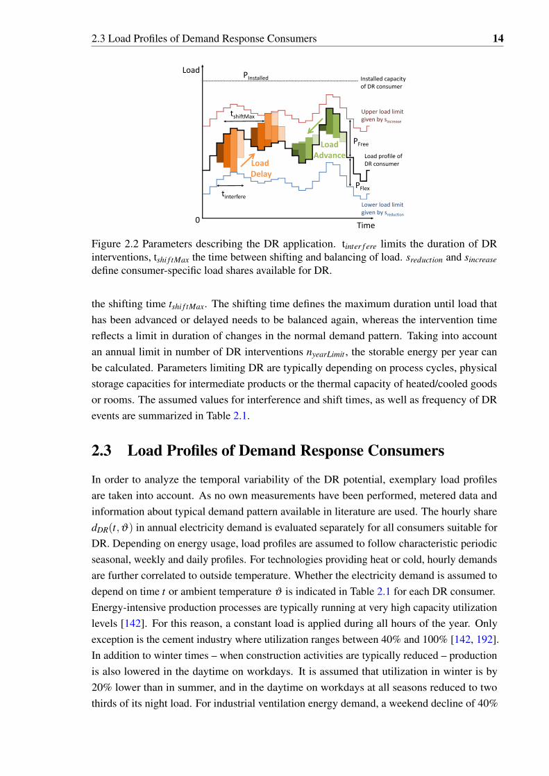
2.3 Load Profiles of Demand Response Consumers 14

Time

PInstalled

tshiftMax

tinterfere

PFree

PFlex

Load Delay

Load Advance

Upper load limitgiven by sincrease

Lower load limitgiven by sreduction

Installed capacityof DR consumer

Load profile ofDR consumer

Load

0

Figure 2.2 Parameters describing the DR application. tinter f ere limits the duration of DRinterventions, tshi f tMax the time between shifting and balancing of load. sreduction and sincreasedefine consumer-specific load shares available for DR.

the shifting time tshi f tMax. The shifting time defines the maximum duration until load thathas been advanced or delayed needs to be balanced again, whereas the intervention timereflects a limit in duration of changes in the normal demand pattern. Taking into accountan annual limit in number of DR interventions nyearLimit , the storable energy per year canbe calculated. Parameters limiting DR are typically depending on process cycles, physicalstorage capacities for intermediate products or the thermal capacity of heated/cooled goodsor rooms. The assumed values for interference and shift times, as well as frequency of DRevents are summarized in Table 2.1.

2.3 Load Profiles of Demand Response Consumers

In order to analyze the temporal variability of the DR potential, exemplary load profilesare taken into account. As no own measurements have been performed, metered data andinformation about typical demand pattern available in literature are used. The hourly sharedDR(t,ϑ) in annual electricity demand is evaluated separately for all consumers suitable forDR. Depending on energy usage, load profiles are assumed to follow characteristic periodicseasonal, weekly and daily profiles. For technologies providing heat or cold, hourly demandsare further correlated to outside temperature. Whether the electricity demand is assumed todepend on time t or ambient temperature ϑ is indicated in Table 2.1 for each DR consumer.Energy-intensive production processes are typically running at very high capacity utilizationlevels [142]. For this reason, a constant load is applied during all hours of the year. Onlyexception is the cement industry where utilization ranges between 40% and 100% [142, 192].In addition to winter times – when construction activities are typically reduced – productionis also lowered in the daytime on workdays. It is assumed that utilization in winter is by20% lower than in summer, and in the daytime on workdays at all seasons reduced to twothirds of its night load. For industrial ventilation energy demand, a weekend decline of 40%

2.4 Quantification of Flexible Loads 15

(Saturday) and 50% (Sunday) is assumed; commercial ventilation is furthermore reduced by50% at night-time. The electricity demand of cooling appliances in private homes, retailing,hotels and restaurants is estimated to be by 10% lower in winter times than in summer; itadditionally declines by 20% at night, given that the frequency of user interventions tendsto go down. Based on metered data presented in [146], cold storages and industrial coolingare assumed to have lower demands on Saturdays (-5%), Sundays (-10%) and during peaknetwork load hours in the morning (-50%). Pumps in the fresh water supply are also typicallyrunning during off-peak hours at night; here it is assumed that load is reduced by two thirdsin the daytime. The operation of washing machines, tumble dryers and dish washers is mainlydriven by the daily routine of its users; Prior [148] provides measured hourly usage profilesfor different weekdays and seasons, which are used here. All periodical load profiles aresummarized in Table A.1 to A.3 in Appendix A.

The energy demand of space and water heating, as well as air conditioning is stronglycorrelated to outside temperature. All technologies with temperature-dependent demandare assumed to follow the country-specific heating and cooling profiles obtained using themethodology introduced in Section 3.3 of this work.

2.4 Quantification of Flexible Loads

2.4.1 Industrial Demand Response PotentialsEnergy-intensive Processes

DR potentials in energy-intensive industries are estimated based on production capacitiesAyear and specific energy demands Wspec found in literature and statistics. Annual electricitydemands Wyear and installed electrical capacities PmaxCap of each DR process I are calculatedaccording to Eq. 2.1 and 2.2, taking into account the capacity utilization level sutil , totalnumber of hours of the year and revision outages frevision. Most industrial processes areoperated at utilization levels below 100%; the actual production is consequently lower thanthe maximum production capacity. It is assumed that the production capacity reflects thequantity that can be manufactured if the unit is running at full load at all times except for itsannual revision.

W Iyear = AI

year ·W Ispec · sI

util (2.1)

PImaxCap =

W Iyear

8760h ·(1− f I

revision)· sI

util(2.2)

The potential load reduction Pf lex(t) in each hour is given by the difference between currentload and minimum load of the process (see Eq. 2.3). Its value changes during the yearaccording to the hourly demand share d(t). The minimum process load is defined relativeto the installed electrical capacity and given by parameter smin. The potential load increasePf ree(t) is calculated from the difference between maximum load and current load, which is


at least temporarily greater than zero for all processes operated at less than 100% utilization.This difference is multiplied with parameter sincrease, reflecting the free production capacityshare available for DR (see Eq. 2.4). Table 2.2 summarizes the assumed parameter values ofall DR processes.

PIf lex(t) = dI(t) ·W I

year︸︷︷︸Load in hour t

−PImaxCap · sI

min︸︷︷︸Minimum Load

(2.3)

PIf ree(t) = (PI

maxCap ·(1− f I

revision)︸︷︷︸

Maximum Load

−dI(t) ·W Iyear)︸︷︷︸

Load in hour t

· sIincrease︸︷︷︸

Shiftable share

(2.4)

Table 2.2 Parameter used for the calculation of DR potentials in energy-intensive industries.

Process Ayear Wspec frevision sutil smin sincrease ReferencesMt/a kWh/a % % % %

Aluminum electrolysis 3.8 14000 5% 100% 75% 0% [110, 142, 149, 190]Copper electrolysis 3.1 350 5% 95% 75% 0% [44, 110, 190]Zinc electrolysis 2.1 3400 5% 100% 75% 0% [44, 78, 110, 190]Electric steel production 90 525 5% 100% 0% 0% [142, 190, 196]Chloralkali - membrane 6.5 2100 5% 95% 50% 0% [56, 110, 137]Chloralkali - mercury 4.1 3600 5% 95% 30% 0% [56, 110, 137]Mechanical wood defibration 19 1500 5% 80% 0% 100% [19, 110, 142, 189]Wastepaper processing 72 250 5% 80% 0% 100% [19, 20, 110, 162, 189]Paper machines 118 425 5% 90% 70% 100% [36, 110, 189]Cement mills 338 110 5% 80% 50% 100% [142, 190, 191]Calcium carbide production 0.4 3100 5% 80% 0% 100% [23, 85]Air separation - Oxygen 23 238 5% 80% 60% 100% [91]Air separation - Nitrogen 14 160 5% 80% 60% 100% [91]Air separation - Argon 8 224 5% 80% 60% 100% [91]

Industrial Cross-sectional Technologies

Flexible loads in the cross-sectional technologies cooling and ventilation are evaluated basedon their annual electricity demand Wyear. These demands are estimated using data from[51, 150, 179]. Dividing Wyear by the number of full load hours nFLH , the installed capacityis obtained (see Eq. 2.5). In contrast to energy-intensive processes, no revision outage isconsidered.

PImaxCap =

W Iyear

nIFLH

(2.5)

In the assessment of potential load reduction and increase, fixed shares in current load sreduction

and unused capacity sincrease available for DR are assumed. They allow for the calculation ofpotential load reduction and increase according to Eq. 2.6 and 2.7. The upper limit of thelatter is set by the installed capacity. Estimated energy demands, utilization levels and DR


shares of the industrial cross-sectional technologies are summarized in Table 2.3.

PIf lex(t,ϑ) = dI(t,ϑ) ·W I

year︸︷︷︸Load in hour t

· sIreduction︸︷︷︸

Shiftable share

(2.6)

PIf ree(t,ϑ) =

(PI

maxCap −dI(t,ϑ) ·W Iyear)︸︷︷︸

Unused Capacity

· sIincrease︸︷︷︸

Shiftable share

(2.7)

Table 2.3 Parameter used for the calculation of DR potentials in industrial cross-sectionaltechnologies.

Process Wyear nFLH sreduction sincrease ReferencesTWh/a h/a % %

Cooling in food industry 31 5,840 50% 90% [110, 150, 176, 179]Building Ventilation 12 7,008 50% 0% [51, 110, 150, 176, 179]

2.4.2 Flexible Loads in the Commercial Sector

Commercial sector DR potentials are available in the supply of cold, heat, water and ventila-tion, as well as in waste water treatment. Flexible loads in these applications are calculatedbased on their annual energy consumptions Wyear. In the absence of country-specific data, theyare approximated by multiplying the commercial sector demand Wcom from [61, 100, 101]with average demand shares scom of the relevant uses (see Eq. 2.8). According to survey datapublished in [17], 19.7% of the 2007 commercial sector electricity consumption in EU-27countries was used for the supply of space heat and hot water, 12.6% for ventilation, 5.9%for pumps, 8.7% for cooling appliances and 2.9% for air conditioning. All other uses are notrelevant to DR. With exception of space heating and air conditioning, which are assumed todepend on outside temperature, these shares are applied to all European countries. Pursuantto values estimated for Germany in [179], the electricity demand of cooling appliances issubdivided into food retailing (75%), cold storages (10%) and hotels/restaurants (15%).

W Iyear =Wcom · sI

com (2.8)

The air conditioning share in the sectoral demand sACdemand is approximated using long-term

average cooling degree days (CDD) of each country [12]. It ranges between 0.5% in northerncountries to 12% on the Mediterranean islands (see Table 2.4 and Table A.6in Appendix A).These values rely on shares available for a number of countries on the one hand and the overallenergy demand of air conditioning on the other. In the assessment of air conditioner andresidential heat circulation pump full load hours, in addition to heating degree days (HDD)and CDDs, demand profiles for heat and cold are taken into account. Their calculation isdescribed in Section 3.3. It is assumed that whenever the cooling demand surpasses 60% of


its peak value, the overall air conditioner park is running at the maximum load of 75% ofits installed capacity. For lower demands, capacity utilization reaches 1.25-times the ratiobetween current and peak load. Resulting full load hours range between 136 in Estonia and991 in Cyprus, with a European average of 467 hours (see Table A.6 in Appendix A). Incountries without CDD, it is set to 100 hours/year.

Table 2.4 Air conditioning (AC) share in commercial electricity demand.

Annual number of CDD sACdemand

<100 0.5%<200 1.0%<300 2.0%<400 3.0%<500 4.0%<600 5.5%<700 7.0%<800 8.5%<1000 10.0%≥ 1000 12.0%

Annual full load hours (FLH) of hot water boilers nHWFLH and storage heaters nSH

FLH areestimated for each country based on long-term average HDD collected by [59] (see Table A.6in Appendix A). It is assumed, that the utilization is higher in colder climates according to thevalues in Table 2.5.

Table 2.5 Assumed annual full load hours for storage water heater (WH) and storage heater(SH).

Annual number of HDD nHWFLH nSH

FLHh/a h/a

≤ 1000 175 200≤ 2000 200 350≤ 3000 225 500≤ 4000 250 650> 4000 275 800

With the annual electricity demands and FLH summarized in Table 2.5, the installedcapacity is calculated according to Eq. 2.5. No procedural limitations of load shifting areconsidered in the commercial sector. Load shares sreduction and sincrease available for DR arethus set to 100% of current load and unused capacity, respectively. Only exception is thewaste water treatment, where pursuant to [88, 121] values of sreduction=20% and sincrease=50%are applied. Based on annual demand, installed capacity and hourly load profiles, possibleload reduction and increase are calculated according to Eq. 2.6 and 2.7, respectively.

2.4.3 Flexible Loads in the Residential Sector

Residential load shifting is evaluated for heating, cooling, air conditioning and washingequipment. The latter comprises washing machines, tumble dryers and dish washers. In


Table 2.6 Parameter used for the calculation of commercial sector DR potentials.

Process scom nFLH References% h/a

Cooling in food retailing 6.5% 5840 [17, 110, 176, 179]Cold storages 0.9% 5000 [17, 110, 176, 179]Cooling hotels/restaurants 1.3% 5000 [17, 110, 176, 179]Ventilation 12.6% 4380 [17, 110, 150]Air conditioning see Table A.6 [17, 176]Storage water heater 1.5% see Table A.6 [17, 164]Storage heater country valuesa own assumptionsPumps in water supply 3% 4380 [38, 120]Waste water treatment 3% 5694 [88, 121]

a Due to limited data availability only considered in Germany (scom=2%,nFLH=650 h/a) and France (scom=5%, nFLH=500 h/a).

contrast to the other sectors, residential DR loads are quantified in a bottom-up approach.Household numbers nHH and country-specific equipment rates feq of relevant devices areobtained from [36, 51, 72, 97, 123, 170], or approximated using available data (see Table A.6in Appendix A). Multiplying the resulting unit number with the specific capacity Punit andenergy consumption Wunit , country sums are calculated for each appliance type accordingto Eq. 2.9 and 2.10. Based on [17, 134], an annual refrigerator and freezer unit demand of350 kWh is applied. For washing equipment, average power demands during use Pcycle, aswell as frequency ncycle and duration of use ∆tcycle are taken into account (see Table 2.7).Relying on measured consumption data from [70, 165], annual demands are calculated (Eq.2.11).

PImaxCap = nHH · f I

eq ·PIunit (2.9)

W Iyear = nHH · f I

eq ·W Iunit (2.10)

W Iunit = PI

cycle ·∆tIcycle ·nI

cycle (2.11)

Table 2.7 Parameter used for the calculation of residential sector DR potentials.

Device Wunit Pcycle ∆tcycle ncycle ReferenceskWh/a kW h 1/a

Washing machines 219 0.75 2 146 [51, 165]Laundry drier 306 1.5 2 102 [51, 165]Dish washer 270 0.65 2 208 [51, 70, 165]

In the calculation of annual space heating, hot water generation and air conditioningelectricity consumption, unit capacities Punit are multiplied with estimated FLH nFLH (Eq.2.12).

W Iunit = PI

unit ·nIFLH (2.12)

2.5 Extrapolation of Flexible Loads 20

Average capacities per dwelling are assumed with 1.65 kW for air conditioners, 2 kW forelectric storage water heaters, 100 W for heat circulation pumps and 14 kW for electric storageheaters [17, 170, 176, 178, 195]. Country-specific air conditioner, water heater and storageheater FLH are obtained as described in Section 2.4.2. In the calculation of heat circulationpump FLH, an approach similar to that used for air conditioners is chosen. According to[176, 178], average annual operation time of heat circulation pumps in Europe is around5000-6000 hours. This implies that not all pumps are switched off in summer. Here, a baseload of 25% of the installed capacity is assumed for all countries. This base load is assignedto all hours with a demand below 15% of the annual peak. For higher demands, the loadis assumed to be 1.67-times the ratio between current and peak load. If this ratio is higherthan 0.6, circulation pumps are assumed to run at full load. It is assumed that all devicesare available for DR; sreduction and sincrease are thus set to 100%. Hourly load increase anddecrease are then obtained using Eq. 2.6 and 2.7.

2.5 Extrapolation of Flexible Loads

DR potentials are also quantified for the scenario years 2020, 2030 and 2050. Therefore,the parameters defining flexible loads are extrapolated. They include industrial productionoutput and specific demands, commercial sector electricity demand structure, as well asresidential appliance energy consumption and equipment rates. Extrapolations are mostlybased on statistics of recent developments. No changes in periodic load profile componentsare taken into consideration. However, outside temperature dependent profiles are affected bythe assumed changes in heating and cooling limit temperature, described in Section 3.3.

Table 2.8 summarizes the applied changes in industrial production output ∆Ayear, as wellas output specific electricity demands ∆Wspec. Changes in overall production have beenderived from an analysis of global and European industry statistics. All output reductionand increase is equally distributed over all current production sites, since shut-downs andnew installation of factories cannot be anticipated. Constant changes in output are assumed,cyclical economic upturns and downturns are neglected. Given the high share of energy inoverall production cost, efficiency is of high importance in the energy-intensive industries.Consequently, efficiency improvements are considered for all processes. The assumptions arebased on past efficiency gains, as well as current best available technologies benchmarks. Withno historical time series data available, energy demands of industrial cooling and ventilationare assumed to remain constant.

Future commercial sector DR potentials are influenced by the development of the overallsectoral demand on the one hand, and the demand shares of the relevant technologies onthe other. According to the framework scenario used in the model application introduced inSection 5.2.2 of this work, the commercial sector final energy demand for electricity in theconsidered countries is assumed to increase by around one third on average until 2050. Apeak value is assumed to be reached in 2040, afterward the trend is reversed. Country values

2.5 Extrapolation of Flexible Loads 21

Table 2.8 Assumptions of future production capacities and specific energy demands ofindustrial DR consumers.

Process ∆Ayear ∆Wspec

%/a %/aElectrolytic primary aluminum -0.5%/a -0.5%/aElectrolytic copper refinement ± 0 -0.3%/aElectrolytic zinc production ± 0 -0.3%/aElectric arc steelmaking +0.5%/aa -0.5%/aChloralkali process -0.2%/ab -0.5%/aCement mills ± 0 -0.5%/aMechanical wood pulp process ± 0 -0.3%/aRecycling paper processing +1.9%/ac ± 0 d

Paper machines +1.1%/ae -0.3%/aCalcium carbide production -1%/a -0.3%/aCryogenic air liquefaction +0.5%/a -0.3%/a

a Additional to the growth of overall European produc-tion, it is considered that the share of electric steelincreases linearly from 39% in 2005 to 75% in 2050.

b It is assumed that all European Chlorine productionis converted to the more efficient and less pollutingmembrane cell method until the year 2030.

c Increase by 3%/a until 2020, and then by 1.5%/a.d Efficiency gains are assumed to be balanced by a

higher energy demand of multiple recycling pro-cesses.

e Increase by 1.5%/a until 2020, and then by 1%/a.

in 2050 range from 66% to 300% of the demand measured in 2010. Table A.5 in AppendixA provides all country-specific demand data. The consumption of cooled and frozen goodshas increased in the past [39]. This trend is assumed to continue, causing an increase ofthe cooling share in commercial demand from 8.7% in 2010 to 10.0% in 2050. Also theventilation share in sectoral demand is assumed to grow slightly, from 12.6% in 2010 to 13.0%in 2050. A steeper increase in demand is applied to air conditioning electricity demand: itsshare is assumed to reach 150% of the 2010 value in all countries. The electricity demandof electric water heating is assumed to decrease by 40% until 2050, due to fuel change andefficiency increase. The reduction is however compensated by a higher share of water heatersequipped with a storage – a doubling from 30% in 2010 to 60% in 2050 is assumed [107]. The2010 electric storage space heater shares of 5% in France and 2% in Germany are assumedto decrease by 0.75% and 0.5% per decade, respectively. In Germany, the technology iscompletely phased out by 2040, in France, the decrease accelerates after 2030 and diminishesto a demand share of 1% in 2050. Also, the shares of water supply and waste water treatmentare assumed to go down in the future – from 3.0% in 2010 to 2.5% in 2050. If not noteddifferently, all changes in demand shares are linearly extrapolated.

Residential DR potentials are strongly correlated to appliance equipment rates. In recentyears, equipment rates of cooling and washing appliances have been stagnating in centraland northern European countries [51]. Here, it is assumed that this level of saturation is

2.6 Geographic Allocation of Flexible Loads 22

reached all over the continent until the year 2050. The equipment rates of residential storagespace heaters are assumed to diminish in all countries to 1% by 2050. Electric storage waterheating usage is also decreasing, but to minor extent. In contrast, equipment rates of heatcirculation pumps are expected to rise. Country-specific values for the year 2050 can beobtained from Table A.6 in Appendix A. All equipment rates are assumed to change linearlyover 40 years. Duration and frequency of washing equipment usage are kept constant for allscenario years, their average load is however assumed to decrease, such as the unit capacitiesof air conditioners and heat circulation pump and the annual energy consumption of coolingappliances (see Table 2.9). Future reductions in appliance energy demand are estimated basedon [193].

Table 2.9 Assumed future domestic appliance characteristics.

Device Parameter unit 2010 2020 2030 2050Refrigerator/Freezer Wunit kWh/a 350 250 175 100Washing machines Pcycle kW 0.75 0.55 0.40 0.30Laundry drier Pcycle kW 1.50 1.25 1.05 0.70Dish washer Pcycle kW 0.65 0.50 0.40 0.30Air conditioner Punit kW 1.65 1.50 1.35 1.10Heat circulation pumps Punit W 100 80 60 20

2.6 Geographic Allocation of Flexible Loads

The spatial distribution of DR potentials is assessed using high resolution GIS data andindustrial production statistics. Population density and land use data allows for the allocationof flexible loads to grid cells of 0.0083° side length. At the equator, this corresponds toapproximately one kilometer, in the investigation area the cell area ranges from 0.27 to0.74 km2.In energy-intensive industries, an identification of individual production plants is pursued.Geographic coordinates of facilities are determined, allowing for a detailed spatial allocationof flexible loads. Based on [190] and different industry associations, the production sites ofaluminum, electric steel, copper, zinc, chlorine, calcium carbide and partially also cementindustry are identified. The exact assignment of production capacities to factories cannotin all cases be extracted from statistics and are estimated where necessary. The remainingindustrial DR potentials are allocated according to employment statistics of Eurostat, whichare available for dedicated sectors and on NUTS-3 statistical region scale [60, 62].4

Given the high number of commercial sector consumers, a geographic allocation cannotaccount for individual sites. Instead, high resolution GIS data containing residential andcommercial areas is used. Corine Land Cover provides European land use data in a spatial

4The initials NUTS are an abbreviation for ’Nomenclature of Statistical Territorial Units’. It is a hierarchicalsystem for dividing up the economic territory of the European Union into smaller units, usually administrativedistricts within member countries. NUTS-2 regions are typically states, NUTS-3 regions counties. For details,see [63].

2.7 Resulting Theoretical Demand Response Potentials 23

resolution of 100 meters [45]. It assigns each grid cell to one of 44 land use classes includingsettlement areas, agricultural use, forest and waterbodies. Here, only the categories continuousurban fabric, discontinuous urban fabric and industrial or commercial units are taken intoaccount. The commercial sector DR potentials are equally distributed over all grid cells ofthese classes.

Residential DR potentials are allocated according to the population distribution. A populationdensity map is provided by the Joint Research Centre (JRC) [76]. The map is scaled withregional Eurostat population statistics and prospects [61] containing data for all scenario years.With this approach, changes in the overall number of inhabitants only affect the populationdensity in communities and not their spatial extension and distribution. Within each region,the population is allocated according to the JRC data.

2.7 Identified Theoretical Demand Response Potentials

2.7.1 Flexible Loads by Technology, Demand Sector and Country

Relying on the methodology and data presented, substantial amounts of flexible loads areidentified. Aggregated over all countries and consumers, the hourly average load reductionpotential through shedding and shifting adds up to 101 GW. With the assumed hourly loadprofiles, in the course of the year its value varies from 64 GW to 161 GW. Highest potentialsare found in the residential sector, lowest in industry: annual averages reach around 21 GWin industry, 30 GW in commercial sector and 49 GW in residential sector. In industry, thereduction potential is almost constant throughout the whole year, whereas it ranges between19 GW and 74 GW in commercial and 20 GW and 106 GW in residential sector.

0%

20%

40%

60%

80%

100%

Austria

Belgium

Bulgaria

Croatia

Cyprus

Czech Re

p.De

nmark

Estonia

Finland

France

German

yGreece

Hungary

Ireland

Italy

Latvia

Liechten

stein

Lithuania

Luxembo

urg

Malta

Nethe

rland

sNorway

Poland

Portugal

Romania

Slovakia

Sloven

iaSpain

Swed

enSw

itzerland UK

Sectoral sh

are in to

tal

potential

IndustryCommercialResidential

Figure 2.3 Sectoral shares in average load reduction potential by country.

The overall free load fluctuates between 742 GW and 839 GW, with an average of 803 GW.These very high values are linked to the overall installed electric capacity of the processesand appliances considered. This is particularly important in the residential sector, wherecooling, heating, air conditioning and washing equipment account for theoretical load increasepotentials of up to 681 GW. In comparison, free loads are much lower in the other demandsectors; in commercial sector they are found to vary between 102 GW and 156 GW, in industrybetween 2 GW and 8 GW, with average values of 145 GW and 5 GW, respectively.


0

1

2

3

4

5

Alum

inum

Copp

erZinc

Chlorin

ePu

lpPape

rRe

cycling pape

rCe

men

tCalcium carbide

Air sep

eration

Ind. coo

ling

Ind. ven

tilation

Cold storages

Cooling ho

tels

Com. stor. ho

t water

Pumps water su

pply

Wastewater treatm

ent

Res. stor. hot waterLoad

redu

ction in GW

Load Reduction MinLoad Reduction MaxLoad Reduction Average

01020304050607080

Electric steel

Cooling retailing

Com. V

entilation

Commercial AC

Com. storage heater

Freezers/refrig

erators

Washing

machine

sTumble dryers

Dish washe

rsRe

side

ntial A

CRe

s. storage he

aters

Heat circulation pu

mpsLoad

redu

ction in GW Load Reduction Min

Load Reduction MaxLoad Reduction Average

Figure 2.4 Average load reduction potential by technology. Note that left and right graph havedifferent y-axis scale.

The share each demand sector holds in the yearly average of flexible loads shows sig-nificant differences between countries (see Figure 2.3). The residential share ranges from15% in Luxembourg to 70% in Lithuania, whereas the commercial share varies from 11% inRomania to 52% in Cyprus and the industrial share from 2% in Malta to 65% in Luxembourg.Free loads are in all countries dominated by residential appliances: they provide over 80% ofthe overall potential, compared to 18% in commercial sector and 1% in industry.

0

2

4

6

8

10

Load

increase in

GW

Load Increase MinLoad Increase MaxLoad Increase Average

0306090120150180210240

Load

increase in

GW

Load Increase MinLoad Increase MaxLoad Increase Average

Figure 2.5 Average load increase potential by technology. Note that left and right graph havedifferent y-axis scale.

Flexible loads are distributed very unevenly over the 30 processes and appliances analyzed.Taking into account annual averages, highest contributions to the overall reducible load arefound in pulp and paper (6%) and steel (6%) industry, as well as residential space heating(19%), commercial ventilation (13%) and refrigerators/freezers in retailing (6%) and privatehouseholds (14%). Industrial potentials furthermore include considerable loads of cement,aluminum electrolysis, Chloralkali process and cross-sectional technologies. Minor loadreductions can be made available in the copper, zinc, calcium carbide and air liquefactionindustry. The potential load reduction in commercial sector load is dominated by coolingand HVAC appliances, with smaller contributions from public water supply and treatment.


In residential sector, more than one third of the load reduction can be realized by shiftingelectricity consumption of storage heaters and heat circulation pumps. Cooling and washingequipment provide more than 20% each; lower but still substantial potentials are found for airconditioning and electric water heating. In contrast to the diversified distribution of reducibleloads, free loads can almost completely be attributed to electric space heating (24%), storagewater boilers (21%) and washing equipment (38%). Average, minimum and maximum loadreduction and increase potentials of the dominating technologies are displayed in Figure 2.4and Figure 2.5, respectively. Country values for all technologies are listed in Table A.9 andTable A.10 in Appendix A.

0%10%20%30%40%50%60%70%80%90%

Austria

Belgium

Bulgaria

Croatia

Cyprus

Czech Re

p.

Denm

ark

Estonia

Finland

France

Germany

Greece

Hungary

Ireland

Italy

Latvia

Lithuania

Luxembo

urg

Nethe

rland

s

Norway

Poland

Portugal

Roman

ia

Slovakia

Sloven

ia

Spain

Swed

en

Switzerland UK

Load

redu

ction to peak load Minimum load reduction potential

Maximum load reduction potentialAverage load reduction potential

Figure 2.6 Minimum, maximum and average load reduction potential relative to the annualpeak load, subdivided by country.

In order to assess the potential contribution of DR to power system stability, load reductionand increase are related to the annual peak load in each country. Figure 2.6 shows the ratiosof annual minimum, maximum and average load reduction potential to the 2010 peak load. Inmost EU countries, the average reduction equals between 10% and 25% of peak load. A lowervalue is found in the Czech Republic, higher in Greece, Luxembourg and Romania. The ratioof maximum load reduction potential to peak load reaches very high values in countries witha widespread use of the electric space and water heating or air conditioning systems, whichare assumed to be available for load shifting. In most countries, the potential load increaseexceeds the 2010 peak load in at least one hour of the year (see Figure 2.7). This again resultsfrom the high overall capacity of residential appliances.

0%

50%

100%

150%

200%

250%

Austria

Belgium

Bulgaria

Croatia

Cyprus

Czech Re

p.

Denm

ark

Estonia

Finland

France

Germ

any

Greece

Hun

gary

Ireland

Italy

Latvia

Lithuania

Luxembo

urg

Nethe

rland

s

Norway

Poland

Portugal

Romania

Slovakia

Sloven

ia

Spain

Swed

en

Switzerland UK

Load

increase to

peak load Minimum load increase potential

Maximum load increase potentialAverage load increase potential

Figure 2.7 Minimum, maximum and average load increase potential relative to the annualpeak load, subdivided by country.


2.7.2 Temporal Availability of Flexible Loads

The substantial difference between minimum and maximum values of some flexible loadsdisplayed in Figure 2.4 and 2.5 indicates a strong temporal variation in the availabilityof DR potentials. They are particularly pronounced for space heating, ventilation and airconditioning, as well as residential washing equipment. Figure 2.8 illustrates the developmentof the daily load reduction average during one year for five representative technologies. Itreflects the load profiles assumed in Section 2.3. With no load changes considered, DRpotentials in energy-intensive industries – here the aluminum electrolysis is shown exemplary– are constantly available throughout the whole year. Also the power demand of retail coolingshows only minor variations. In contrast, shiftable loads in the provision of air conditioningand space heating are strongly influenced by outside temperature and have annual load curvescontrasting each other. Particularly in air conditioning demand, where short-term reactions totemperature occur, high peaks in single days and hours can be observed. The variations inthe load reduction potential profile of commercial ventilation are directly correlated to theassumed weekend demand decline.

0

4

8

12

16

20

1 15 29 43 57 71 85 99 113

127

141

155

169

183

197

211

225

239

253

267

281

295

309

323

337

351

365

Load

redu

ction in GW

Day of the year

Commercial ACHeat circulation pumpsAluminium electrolysisCommercial ventilationCooling at retail

Figure 2.8 Daily load reduction average during one year for five representative DR loads.

Due to the high air conditioner share, the annual maximum of the overall theoreticalload reduction potential is reached in summer times. In peak hours, the potential can betwice as high as on average. Hours with lowest reduction potential are found in the transitionperiod between winter and summer, when both air conditioner and heat circulation use is low.Average daily reduction potentials are found to be lower on weekends than on working days.This results from reduced industrial and commercial demand.

0

4

8

12

16

20

3360

3365

3370

3375

3380

3385

3390

3395

3400

3405

3410

3415

3420

3425

3430

3435

3440

3445

3450

3455

3460

3465

3470

3475

3480

3485

3490

3495

3500

3505

3510

3515

3520

3525

Load

redu

ction in GW

Hour of the year

Commercial ACHeat circulation pumpsDish washersCommercial ventilationPumps water supply

Figure 2.9 Daily load reduction average during one week for five representative DR loads.


0%

20%

40%

60%

80%

100%

1 15 29 43 57 71 85 99 113

127

141

155

169

183

197

211

225

239

253

267

281

295

309

323

337

351

365

Load

redu

ction po

tential

relativ

e an

nual m

axim

um

Day of the year

Finland GermanySpain United KingdomItaly

0%

20%

40%

60%

80%

100%1 15 29 43 57 71 85 99 113

127

141

155

169

183

197

211

225

239

253

267

281

295

309

323

337

351

365

Load

increase poten

tial

relativ

e an

nual m

axim

um

Day of the year

Finland Germany Spain United Kingdom Italy

Figure 2.10 Daily load reduction (above) and increase (below) average during one year forfive selected countries relative to the annual maximum.

The flexible load is varying considerably also within each day. This is illustrated fora selection of consumers and a representative spring week in Figure 2.9. Again, the DRpotential provided by industry and cooling appliances is fairly constant throughout the day.The same applies to residential heat circulation pumps. In contrast to that, the DR availabilityof washing equipment, air conditioners and fans is heavily fluctuating. Due to the typicalutilization cycles driven by daylight, working hours and temperature, potentials are mostlyavailable during daytime. This coincides with the overall system load pattern.

The temporal availability of load flexibility arises from the composition of the overallDR potential. Differences between countries are primarily associated to the fraction of spaceheating and air conditioning. Figure 2.10 includes profiles for load reduction and increase infive representative European countries, normalized to the corresponding maximum potential.In northern European countries, the load reduction potential is higher in winter, whereasstrong summer peaks can be observed in Spain and Italy. In Germany, where the industrialshare in the potential is comparatively high, daily averages of load reduction show lowestfluctuations during the year. Also the load increase potentials are is driven by electric heatingdemands: they are approximately by factor two higher in winter than in summer.

2.7.3 Spatial Distribution of Flexible Loads

DR potentials are concentrated to centers of population and energy intensive industry produc-tion. Figure 2.11 shows the potential load reduction density in each grid cell. Major cities andurban agglomerations can be easily identified there.

For further analysis of the spatial allocation of flexible loads, sums over each NUTS-3statistical region are formed, and average values per km2 and inhabitant are calculated. The


Figure 2.11 Density of the load reduction potential in kW/km2.

Figure 2.12 Regional density of the load reduction potential in kW/km2.

Figure 2.13 Average per capita load reduction potential of each NUTS-3 region in kW.

regional density of load reduction potentials is displayed in Figure 2.12. It reaches high valuesnot only in densely populated regions, but also those with a concentration of energy intensiveenergies. The highest values of more than 900 kW/km2 are found in Paris, Inner Londonand the industrial city of Ludwigshafen am Rhein in Germany. Comparatively low densities


are present in sparsely populated areas, for example in north-eastern Germany, Scotland ornorthern Finland, Norway and Sweden. Taking into account population density, regions withhigh industrial and commercial DR potentials can be identified. In Figure 2.13, the per capitaload reduction is shown for each region. Comparatively high values are found for example inthe French region of Aquitaine, the Norwegian coast and Luxembourg.Given that most increase potential through advancing load is provided by residential appli-ances, the geographic distribution is very similar to the population density.

2.7.4 Prospective Development of Demand Response Potentials

With the assumed future energy demands of DR consumers (see Section 2.5), a slight decreaseof flexible loads until the year 2050 is obtained. Until 2020, the overall average load reductionpotential increases by 2%, and then starts decreasing to 101% and 90% of the 2010 valuein 2030 and 2050, respectively. Trends are different for the DR appliances and processesconsidered. Flexible loads are strongly increasing in paper and steel industry, as well as airconditioning, whereas they are significantly decreasing in electric space heating appliances(see upper diagram in Figure 2.14). The composition of national DR potentials determineshow overall flexible load develops in the future. Due to the dominance of the steel industry inthe DR potential, Luxembourg sees a steep increase in flexible load. In contrast, it is reducedby more than one fourth in countries with cold climates and comparatively high electricheating shares, including Austria, Norway and Switzerland (see lower diagram in Figure2.14).

0%

50%

100%

150%

200%

250%

Potential relative to 201

0 value

2010 2020

2030 2050

0%20%40%60%80%100%120%140%160%180%

Austria

Belgium

Bulgaria

Croatia

Cyprus

Czech Re

p.De

nmark

Estonia

Finland

France

Germany

Greece

Hungary

Ireland

Italy

Latvia

Liechten

stein

Lithuania

Luxembo

urg

Malta

Nethe

rland

sNorway

Poland

Portugal

Romania

Slovakia

Sloven

iaSpain

Swed

enSw

itzerland UK

Potential relative to 2010 value 2010 2020

2030 2050

Figure 2.14 Future load reduction potential relative to 2010 values; subdivided by consumer(above) and country (below).

2.8 Summary and Discussion 30

2.7.5 Demand Response Energy Storage Size

The load shifting potential is dominated by customers allowing only short interventions andshifting times (see Table 2.1). They include cooling processes in all sectors, air conditioning,ventilation, heat circulation pumps, fresh water supply and waste-water treatment. All theseappliances can be interrupted for only one or two hours, and the reduced load typically needsto be recovered within the same time span. This limits the storage period of the functionalstorage provided by DR. Depending on the hour of the year, the energy that within two hourscan be charged into the virtual storage by load reduction ranges from 43 GWh to 128 GWh.The temporal variation in storage capacity is correlated to the assumed load profiles ofconsumers participating in DR. The discharging has to begin immediately afterwards and isalso limited to a duration of two hours.Longer intervention times are found for washing equipment, as well as residential andcommercial electric space and water heaters. With the assumed charging durations of up totwelve hours for electric heat production and six hours for washing equipment, the energystorage capacity is comparatively high. Due to its dependency on outside temperature andappliance usage pattern, it shows strong variations between 17 GWh and 707 GWh. Storagecapacity of washing equipment load shifting can reach up to 207 GWh during daytimeand goes down to zero at night. The much better storage function of washing and heatingequipment comes along with shortcomings concerning acceptance and efficiency, respectively.With an assumed maximum shifting time of 24 hours, industrial DR provides medium termstorage. According to the calculated load reduction potentials, between 59 GWh and 65 GWhcan be stored within the applied maximum intervention time of four hours. Given thatindustrial DR includes load shedding, only between and 25 GWh and 31 GWh of the storeddemand has to be recovered within the following 24 hours.

2.8 Summary and Discussion

In this chapter, an assessment of theoretical DR potentials in Europe is presented. It includes30 electricity consumers across all demand sectors, which can shift or shed their load forat least one hour. Special attention is given to the evaluation of temporal availability andgeographic allocation of qualified consumers. The developed methodological framework caneasily be adapted to other world regions or more detailed input data.The analysis reveals substantial theoretical DR potentials in all demand sectors. By sheddingor shifting, an average load reduction of around 100 GW can be achieved. This average valueis equivalent to roughly one third of the minimum and one sixth of the peak load measuredin the investigation area in 2010. Due to the changing load of the flexible consumers, thepotentials show extensive variations during the course of the year. With the assumed demandprofiles, the reducible load varies from 64 GW to 161 GW. The temporal availability offlexible loads is particularly important in residential and commercial sector, where in somehours of the year the summarized reduction potentials drop to less than 20% of their respective


annual maximum value. The annual curve of available DR potential is flatter in countries withhigh industrial shares. In contrast, variations are particularly pronounced in countries withgreat amounts of electric heating and air conditioning.

Residential and commercial load shifting are almost not limited by the available free capacityof DR appliances. Installed and unused capacities in the range of several hundred GWare available; the average load increase potential accounts for 803 GW. It is dominatedby residential and commercial cooling, heating, air conditioning, ventilation and washingequipment, whereas industrial processes contribute less than 1% of the overall amount. Thesevery high potentials of load increase could, however, only be accessed, if loads could beshifted without any temporal limitations. Given that load shifting is affected by the demandprofiles of the corresponding consumers, as well as upper limits in shifting time, the overallfree capacity can only be used to limited extent. Only those devices that would regularlyrun within the previous or following tmaxShi f t hours are available in each hour. Especiallyresidential load shifting is typically not limited by the available free capacities, but by thereducible capacities. In the evaluation of the calculated theoretical potentials, it needs tobe taken into account that both load and DR potential of subsequent hours are influencedwhenever a load reduction or increase is called. All shifted demand needs to be balancedwithin a given period of time, thus increasing or decreasing the load in one or several followinghours. Potential load reduction and increase in each hour are not only correlated to the DRconsumer demand profiles, but also to each other. Limitations in duration and frequency ofDR interventions pose additional restrictions.

In the evaluation of the findings of this chapter it has to be considered that this assessment islimited to theoretical potentials. Restrictions in DR use resulting from the manifold technical,economic, legal and societal barriers have been disregarded completely. Additionally, thestated potentials include also those consumers that are already participating in DR programs,which might further reduce the accessible DR resources. On the other hand, the usage of on-site power generation could allow for additional grid load reductions, which are not taken intoaccount here. The same applies for further consumers with demand flexibility not included inthis assessment, as well as increased industrial demand flexibility provided by the installationof physical storage for intermediate products.

The results of this assessment rely on numerous assumptions and simplifications, affectingboth the average potentials and their temporal availability throughout the year. Some of themmight cause an over- or underestimation of the overall potentials, others a wrong distributionto or within the countries in the investigation area. In the absence of detailed statistics, countryand consumer specific peculiarities are considered only to a minor degree. Calculated annualenergy demands of flexible consumers rely on a number of assumptions with significantimpact on the results. This is particularly important in the residential and commercial sector.The use of European averages in the calculation of demand shares of DR appliances in thecommercial sector might relocate a certain share of the potential from one country to another.The same goes for the global assumptions made for the energy demands and usage pattern


of the residential washing and cooling appliances, which were applied to all countries in theinvestigation area. It has not been considered that the efficiency standard of devices variesbetween countries.Industrial potentials are by large extend based on detailed production statistics. However, theassumed specific energy demands, utilization levels and minimum process loads might notapply to the same extend to all facilities. This is also the case for the annual utilization ofcooling and ventilation equipment in industrial and commercial sector. Another importantassumption is related to the load profiles. Given that no comprehensive database of meteredload was available, exemplary load profiles found in literature were used. Consequently,neither country-specific household activity and appliance usage patterns, nor facility-specificindustrial production cycles are reflected in the resulting hourly potentials. A more detailedanalysis of national or regional DR potentials should rely on a broader database of meteredload profiles, as well as technology and consumption characteristics.The geographic allocation of flexible consumers provides a first approximation of the regionalconcentration of DR potentials. It is detailed and robust for industry, since single productionsites have been identified. Also the usage of population density data for residential DRloads provides a realistic allocation. In contrast to that, the data set used for the commercialconsumers represents a rough simplification of the real demand distribution.The primary focus of this chapter is to gain an overview of the electricity consumers thatmight be used for DR and to provide a first estimate of its loads in Europe. Due to the largenumber of processes, appliances and countries considered, and the lack of country-specificconsumption data, it does not reach the degree of detail of other, more focused studies. Eventhough they rely on various assumptions and approximations, the results of this assessmentoffer an indication in which regions and sectors high amounts of sheddable and shiftable loadscan be accessed, and provide the ground for subsequent studies of the economic benefits ofDR. Given the broad range of flexible loads identified here, it appears attractive to pursueDR programs in all consumer sectors. Whether and to what extent DR can compete withalternative balancing options will be evaluated exemplary for Germany in the REMix-OptiMocase study presented in Chapter 5. It relies on the calculated DR potentials and load profiles,and takes into account the participation of residential and commercial consumers in DRprograms, as well as costs caused by shedding and shifting of loads.

Chapter 3

Heat Demand and TheoreticalCogeneration Potential in Europe

This chapter is focused on the assessment of the European heat demand and cogenerationpotentials. It is subdivided to three sections: in Section 3.1, the European district heating(DH) potential is evaluated relying on a GIS-based approach. The subsequent Section 3.2is dedicated to industrial cogeneration potentials in Europe. Dimensioning and operationof cogeneration (combined heat and power, CHP) plants are closely related to the temporaldevelopment of the heat demand during the year. For this reason, Section 3.3 providesa method for the approximation of high-resolution synthetic heating and cooling demandprofiles. Based on the identified potentials, the contribution of flexible CHP operation to thebalancing of fluctuations in VRE power generation will be analyzed in Chapter 5.

3.1 Quantification of District Heating Potentials

3.1.1 Introduction

Previous studies argue that there are significant possibilities of an extension of DH in mostEuropean countries, however without performing a detailed analysis [52, 194]. Germany’sDH potentials have been quantified in bottom-up approaches making use of building statisticsand satellite data in high spatial resolution [49, 55]. CHP potentials have been furthermorestudied in national studies for the United Kingdom [106], Austria [167] and Denmark [133].Just recently, [28] have presented a method for the quantification of European DH potentialsrelying on an assessment of regional heat demands and excess heat availability.In this section, potentials for an extension of DH in Europe are evaluated.1 Today, the shareof DH in the residential and commercial space and water heating supply reaches over 40% inseveral countries including Denmark, Finland and Sweden [51]. It is mainly used in urbanareas, but also in sparsely populated regions [71, 152]. The spectrum of DH heat sourcesranges from conventional fossil or nuclear fueled power plants to biomass, solar thermal and

1This section is based on previous publications of the author [79, 81]

3.1 Quantification of District Heating Potentials 34

geothermal energy [154]. Thermal waste treatment plants and industrial waste heat recoverycan offer additional heat sources.Even though thermal energy storage (TES) technologies can be integrated independent ofthe heat consumer, its usage appears particularly attractive in DH systems, given the lowerrelative losses of greater storage units and the lower temperature requirements in comparisonto object supply and industrial process heat, respectively. DH storage systems are typicallywater basins or tanks, which feature comparatively simple and well-known technology, as wellas low specific costs. Such storage systems are increasingly becoming an integral part of DHnetworks in different European countries, including Denmark, Sweden, Austria and Germany.However, they are still an exception rather than the norm. Existing DH-TES are used for theprovision of back-up and peak load on the one hand, and for an optimized CHP operation,including reduced part load operation and down-regulation in times of low electricity prices,on the other [8]. In the past, low electricity spot prices have mostly occurred at night andweekends, they are however increasingly correlated to peak generation of VRE [87].The analysis presented in this section is conducted in a spatially explicit top-down approachcomposed of four main steps: (1) an estimation of current and future annual space and waterheating energy demand in the residential and commercial sector on country level, (2) anapproximation of regional differences in specific demands, (3) a consideration of the spatialdemand distribution and (4) an evaluation of the suitability to supply the demand with DH (seescheme in Figure 3.1). The analysis of DH potentials is performed for a total of 31 countries,including all 28 EU member countries, as well as Norway, Switzerland and Liechtenstein.

3.1.2 Current and Future Residential and Commercial Sector Heat De-mand

The technological and economic potential for DH in a specific region is primarily definedby the overall heat demand on the one hand, and the demand density on the other. For thepresent analysis it is assumed that only heat demands in the residential and commercial sectorcan be provided by DH systems. Consequently, it is not accounted for primary and secondarysector demands. All heat demand for space heating (SH) and hot water (HW) generation isaddressed, whereas process heat (PH) in the commercial sector is covered only to a limitedextent. Present heat demands in residential and commercial sector are quantified for eachcountry using detailed energy demand statistics. Its future development is then assessed witha simplified building stock model.

Current Demand

Main data source of residential and commercial energy consumption is the Odyssee energyindicator data base [51]. For all EU countries, as well as Norway and Switzerland, it provideshistorical data of final energy consumption for residential space heating, commercial spaceheating and residential water heating, all subdivided by fuel. It furthermore includes country


Residential Demand Commercial Demand

Regional Temperature Building Type

Population Commercial Areas

1) Per Capita Demand

2) Relative Demand

3) Demand Density

4) District Heating Areas

Figure 3.1 Schematic representation of the procedure in the assessment of DH potentials. Inthe first step, inhabitant-specific annual demands are evaluated (1). They are then weightedaccording to regional climate and building type (2), and spatially distributed using populationand land-use statistics (3). Finally, a minimum demand density is applied in order to obtainpotential DH supply areas (4).


data of dwelling stock and new construction by dwelling type, average floor area and specificspace heat demand of existing and newly built dwellings, as well as total tertiary sector floorarea and employment.2 The database allows for the calculation of four useful energy demandcategories for each country, distinguishing by energy usage (space or water heating) on the onehand, and demand sector (residential or commercial) on the other. Making use of final energydemand fuel shares and fuel specific annual conversion efficiencies, for each country, sectorand usage an average conversion efficiency is estimated. Depending on the correspondingfuel shares, its values ranges from 75% to 90%.3 The database is furthermore used for thecalculation of inhabitant specific floor areas, as well as residential and commercial spaceheating useful energy demands per m2. The area-specific commercial sector space heatingdemand obtained in this manner is however based on the overall useful building area, and notthe heated area. Considering statistics for Germany [21, 49], the heated share in overall floorarea is estimated to 55%. Given that no further data sources could be made available, thisvalue is applied to all countries in the investigation area.The resulting inhabitant-specific residential useful energy demands calculated for the year2008 range from 0.9 MWh/a in Malta to 7.8 MWh/a in Finland. In the commercial sector,inhabitant-specific demands are lower and vary from 0.4 MWh/a in Malta to 2.7 MWh/a inLuxembourg. The substantial differences between countries are related to climate, insulationstandard, living areas as well as commercial sector employment share. Values for each countryare displayed in Figure 3.2.

Estimate of Future Demand

The estimate of future residential and commercial useful energy demand for space heatingrelies on a simplified building stock model realized in a spreadsheet application.4 It takesinto consideration temporal changes in population, inhabitant-specific average floor spacesand area-specific space heat demands in the building stock. Based on specific demandvalues of newly built, renovated and pulled down buildings, as well as rate and extent ofenergy-efficiency retrofits, the model iteratively calculates useful energy demand for spaceheating for each year until 2050. Residential and commercial building stock are treatedseparately, given that area-specific demands and modernization rates are typically different.The model additionally includes useful enery demands for hot water production in residentialand commercial buildings. In the estimate of future of commercial sector demand, alsosectoral employment numbers and heated floor space shares are considered. They are derivedfrom statistical data provided in [51, 59].For the assessment of future space heating demand, assumptions concerning the development

2Inhabitant-specific demand values for Liechtenstein are obtained from national statistics or assumed to beidentical to those found in Austria.

3Assumed average annual conversion efficiency from final energy to useful heat are 65% for coal andbiomass, 75% for Oil, 85% for natural gas and 98% for district heat and electricity

4The building stock model is an enhancement of a limited version for Germany developed by T. Nägler inthe framework of [135].


5.66.4

1.92.7

1.9

4.6

7.5

5.7

7.8

5.05.9

3.1

4.75.5

3.45.1

5.8

3.1

7.2

0.9

4.8

7.5

4.1

1.32.2

3.6 3.9

2.2

6.66.2

5.1

0123456789

Austria

Belgium

Bulgaria

Croatia

Cyprus

Czech Re

public

Denm

ark

Estonia

Finland

France

Germany

Greece

Hungary

Ireland

Italy

Latvia

Liechten

stein

Lithuania

Luxembo

urg

Malta

Nethe

rland

sNorway

Poland

Portugal

Romania

Slovakia

Sloven

iaSpain

Swed

enSw

itzerland UK

Useful heat in

MWh/a/inha

bitant

1.6

2.4

0.70.7

0.6

1.3

2.4

1.4

2.6

1.92.1

1.01.2

1.5

0.8

1.41.5

1.1

2.7

0.4

1.5

2.4

1.2

0.50.5

1.2 1.20.8

2.5 2.5

1.5

0

1

2

3

Austria

Belgium

Bulgaria

Croatia

Cyprus

Czech Re

public

Denm

ark

Estonia

Finland

France

Germany

Greece

Hungary

Ireland

Italy

Latvia

Liechten

stein

Lithuania

Luxembo

urg

Malta

Nethe

rland

sNorway

Poland

Portugal

Romania

Slovakia

Sloven

iaSpain

Swed

enSw

itzerland UK

Useful heat in MWh/a/inha

bitant

Figure 3.2 Inhabitant-specific useful energy demands for space and water heating in the year2008. Values for the residential (above) and commercial sector (below). Note that y-axis havedifferent scaling

of newly built, refurbished and demolished buildings are made. In order to achieve substantialdemand reductions in the building sector, increased retrofit rates and depths are required,as well as steep reductions in specific space heat demands of newly built buildings. Givendivergent trends during the past years, different values are applied for the European OECDcountries on the one hand, and Non-OECD countries on the other (see Table B.1 in AppendixB for the list of countries). Consistent with [135, 163], in OECD Europe a retrofit rate of2%, a retrofit depth of 50%, and a reduction in floor area specific space heat demand ofnewly built buildings to less than 10% of the 2010 value are assumed. In Non-OECD Europea less dynamic development is considered. The specific space heat demand is assumed todecrease to approximately 30% of the 2010 value. Also the building refurbishment rate isranging at a lower level: it rises by 0.25% per decade from 0.75% in 2008 to 1.75% in 2050.Efficiency gains achieved by retrofitting are assumed to 20% in 2008 and 40% in 2050 anda linear increase in between. In both OECD and Non-OECD countries, demolition ratesof 0.5% and 1.5% of the building stock are applied in residential and commercial sector,respectively. Demolished and retrofitted buildings have specific demands equivalent to 120%and 130% of the overall building stock average in the corresponding year. Table B.2 inAppendix B summarizes the assumptions both for OECD and Non-OECD countries. Furtherinput to the buildings stock model are the future development of floor areas, as well as hot


water demands. The trends applied are based on three general assumptions: (1) conditionsin different European countries will converge, (2) energy efficiency will be increased and(3) trends do not or only very slowly go into reverse. Country-specific assumptions canbe obtained from Table B.3 and B.4 in Appendix B. Taking into account improvements inefficiency and changes in fuel use, an increase of the average conversion efficiency (finalenergy to useful energy) to 92% until the year 2050 is assumed in the scenario. A linear trendis applied.Based on these assumptions and the building stock model, future residential and commercialspace and water heating demands are calculated. Figure 3.3 shows the development of thedemand until 2050, relative to 2008 values. For each scenario year and demand sector, thelowest and highest country value is provided, reflecting differences in the trends betweencountries. Table B.5 in Appendix B provides detailed values for each country. Due to thehigh retrofit rate and passive house standard of new buildings, the overall demand in Europeis almost reduced by half until mid-century. The relative demand decrease is higher in thecommercial sector, due to a more frequent building reconstruction and lower floor spaceexpansion in comparison to the residential sector.According to [49], commercial process heat demand includes space and water heating witheach accounting for about 30%. This justifies a consideration of this demand in the assessmentof district heating potentials. Given that no comprehensive data on commercial process heatis available, a simple estimate is made. In 2010, process heat was responsible for around8% of Germany’s commercial sector final energy demand [21]. This value is applied to allcountries and kept constant until 2050. The overall commercial sector energy demand isassumed to decrease pursuant to the Other Sector demand in the global scenario discussedin [183] (see Table B.6 in Appendix B). Different developments are applied to the EuropeanOECD countries on the one hand, and the Non-OECD countries on the other. The resultingdevelopment of commercial sector process heat demand represents a rather ambitious scenarioin terms of efficiency increase, and is as well displayed in Figure 3.3.

0%

20%

40%

60%

80%

100%

120%

2008 2020 2030 2050Heat d

eman

d relativ

e to 201

0 value

Scenario year

Residential SH&HW MaxResidential SH&HW MinCommercial SH&HW MaxCommercial SH&HW MinCommercial PH MaxCommercial PH Min

Figure 3.3 Future development of residential and commercial heat demand. Max. and min.represent the European countries with highest and lowest relative values, respectively.


3.1.3 GIS-based Approach for the Identification of DH PotentialsUsing GIS data, the country heat demands are allocated spatially according to population andland use. Taking into account a minimum heat demand density threshold, agglomerationsare identified and considered as areas suitable for DH. The GIS analysis is mostly performedin Idrisi 15.0, except from some first processing steps done in ESRI Arcview. Heat demandparameters of the areas suitable for DH are extracted from the GIS and further processed ina spreadsheet application to obtain summed-up potentials for each country. In the model,hot water and space heat are considered separately, allowing for a division between ratherconstant base load and temperature- and time-dependent variable load.

Development of a High-Resolution Demand Density Map

Dividing by the population number, country average per-capita values for both space heatingand hot water demand in the residential and commercial sector are obtained from the overalldemands listed in Table B.5 in Appendix B. In some cases, average demand values do notreflect the variety of climatic conditions within a country. For this reason, it is assumedthat within each country the per-capita heat demand for both space heating and hot watergeneration in a particular region N is proportional to the heating degree days (HDD). Statisticaltime series of monthly HDD allows for the calculation of long-time average relative per-capitademands Uspec,rel on the level of NUTS-2 statistical regions [58]. To assure that nationalaverage values of residential per-capita demands are not changed, each region’s HDD numbernHDD is weighted with the regional share npop in national population according to Eq. 3.1.

UNspec,rel =

nNHDD ·∑N nN

pop

∑N(nN

HDD ·nNpop) (3.1)

The annual space heating demand depends not only on outside temperature but also on housingconditions such as dwelling size, inhabitant number, building type, architecture and insulationstandard [49, 109, 171]. The lower surface-to-volume ratio of apartment buildings entails arelatively smaller specific space heat demand per square meter. Consequently, it has to beconsidered that the per-capita heat demand is lower in cities, which are generally dominatedby multi-family apartment buildings. Given that no comprehensive statistics of all relevantparameters is available, it is assumed based on [49, 51, 55] that the per-capita heat demandin multi-family buildings is by 20% lower than in single family buildings. In order to applythis assumption to population density data, limits for the presence of different building typeshave been defined. For all areas with a population density above 5000 inhabitants/km2 it isestimated that all buildings are multi-family homes, whereas areas with a density below 300inhabitants/km2 only host single-family buildings. Between those limits, relative per-capitademands increase linearly. This adjustment is only applied to residential space heating, butnot to commercial heat demand and residential hot water demand. Again, the population ofeach grid cell must be considered in order to keep overall demand constant.The model allows for the consideration of an upper limit in the share of buildings that can be


connected to a DH network without prior conversion of the building’s heating infrastructure.The relevant heat demand can thus be reduced by the share of buildings without central water,steam or air heating system. In this assessment of a theoretical potential, it is assumed thatmost buildings can in principle be accessed: connection rates of 95% in 2010, 96% in 2020,97% in 2030 and 98% in 2050 are applied.

In order to obtain heat density maps, the weighted per-capita demand values are combined withraster data sets representing the spatial distribution of residential and commercial consumers.For residential heat demand, the per-capita demand in each grid cell is multiplied with thenumber of inhabitants of the corresponding cell, which is calculated according to the proceduredescribed in Section 2.6. As for demand response potentials (see Section 2.6), the spatialallocation of commercial heat demand is based on the Corine Land Cover data set [45]. It isassumed that commercial heat demand is distributed equally over all grid cells that have beenassigned to the categories representing continuous urban fabric, discontinuous urban fabricand industrial or commercial units. Therefore, first of all the area share of each 1 km2 cellattributed to one of these three categories is calculated. In the next step, the share of each cellin the total national area is computed. The resulting distribution is weighted with the relativeHDD of each NUTS-2 region, according to Eq. 3.1, and then multiplied with total commercialheat demand. Future changes in land use pattern are not taken into account. By allocatingthe specific demands to residential and commercial areas, heat demand density maps with aspatial resolution of 0.0083°, equivalent to a cell area between 0.27 km2 in northern Norwayand 0.74 km2 in southern Spain, are obtained.5

Identification of Potential District Heating Areas

The derived heat demand maps allow an for identification of areas with high demand densities.A high heat density is crucial for the economic viability of DH systems, given that the overallcosts are dominated by the capital costs of the distribution network. Areas suitable for DH aredetermined by taking into account only those with a density above a certain threshold value.Here, four different threshold values are considered in turn: 4 GWh/km2/a, 7 GWh/km2/a,10 GWh/km2/a and 15 GWh/km2/a. These values have been selected based on an analysisof current DH systems in Europe: on the one hand by linking the measured DH heat supply

5A significant share of DH costs arises from the investment in the pipe network. Installation costs aredifferent between countries, but also within a country, and are depending on the location, geometry, density andstructure of the corresponding settlement [31, 143]. For this reason, a simplified distribution cost assessmentmethod has been implemented in the GIS model. It relies on the assumption that the heat distribution cost perunit of energy delivered is determined by the number of buildings connected, the density of the settlement andthe amount of heat supplied. Based on the total number of buildings in each grid cell, the approximate heatpipe length is calculated. In doing so, it is assumed that specific pipe lengths per building increase for lowerbuilding densities. Dividing the heat demand density by the total network length, the linear heat demand densityis obtained. This value is used for an estimation of the average inner pipe diameter. Finally, investment costs fornetwork and heat substations are calculated based on the linear heat demand density and average pipe diameter,taking into account higher costs in densely populated areas, resulting from more efforts for excavation, roadshutoff, traffic diversion and piping [143]. A comprehensive description and application of this approach canbe obtained from [81]. Given that in this work DH potentials are exclusively used as basis for the technologydevelopment scenario discussed in Chapter 5, DH heat distribution costs are not taken into account.


to the corresponding city areas, on the other hand by comparing DH statistics and resultsof the method presented here. After eliminating all grid cells with a demand density belowthe selected threshold value, neighboring cells of sufficiently high demand are grouped intoagglomerations. In metropolitan areas those agglomerations can have sizes of many squarekilometers, but there are also examples composed of one single cell. For further analysis,each agglomeration is assigned to one or various countries, and its average heat demanddensities, as well as annual space and water heating demands are extracted. Using thesevalues, agglomeration are grouped to classes representing different annual demands and thusthermal loads. Like this, the DH heat supply can later be subdivided to differently sized CHPtechnologies with characteristic techno-economic parameters.

Subdivision of the Potential to DH Size Classes

The DH assessment tool includes an independent model focusing on the supply of theidentified potentials. It allows for an automatic assignment of a CHP technology with peakboiler to each agglomeration, as well as a subsequent calculation of installed capacities,efficiencies, power generation, costs and fuel demands of the supply infrastructure in heat-controlled operation mode. Its output is summarized to countries and technology classes incomprehensive spreadsheet files, containing additional information extracted from the GISmodel, such as agglomeration areas, populations, geographical coordinates and hot waterdemand shares.Based on the annual heat demands, each agglomeration is assigned by the model to one offour DH size classes, characterized by an approximate CHP electric capacity ranging from50 kW-1 MWel , 1-10 MWel , 10-50 MWel and >50 MWel . In order to do so, the annual CHPheat production UCHP of each agglomeration is calculated from the useful energy demandfor space (USH) and water (UHW ) heating, heat distribution losses in buildings λbuilding andnetworks λnetwork and the CHP heat supply share sCHP according to Eq. 3.2.

UCHP =UHW +USH(

1−λbuilding)· (1−λnetwork)

· sCHP (3.2)

Table 3.1 Technology input for the definition of DH size classes.

DH-XL DH-L DH-M DH-SMin. Electric Capacity Pcap,CHP 50 MW 10 MW 1 MW 0.05 MWPower-to-heat ratio σP 1.1 1.0 0.85 0.7Min. Thermal Capacity Qcap,CHP 45.5 MW 10 MW 1.25 MW 0.07 MWFull Load Hours nFLH 4500 4500 4500 4500CHP Supply Share sCHP 0.85 0.85 0.85 0.85DH Network Loss λnetwork 10% 10% 10% 10%DH Building Loss λbuilding 2% 2% 2% 2%Min. Heat Demand UCHP 212 GWh/a 47 GWh/a 5.8 GWh/a 0.33 GWh/a

With approximated CHP full load hours nFLH =UCHP/Qcap,CHP and power-to-heat ratiosσP = Pcap,CHP/Qcap,CHP, thermal Qcap,CHP and electric Pcap,CHP CHP capacities are obtained.


Making use of these capacities, the DH potential is subdivided into four size classes, whichwill later be considered in the definition of a DH scenario (see Appendix E.2). Table 3.1summarizes the assumed technology parameter, as well as the characteristic annual heatdemands and power generation capacities of the size classes.

3.1.4 Resulting District Heating PotentialsTaking into account the demand of the year 2008 and the lowest considered minimum demanddensity of 4 GWh/km2/a, an overall DH potential of 5,792 PJ is identified in the investigationarea. This is equivalent to 53% of the considered residential and commercial heat demand.The 24,232 agglomerations and the supplied heat are distributed rather unevenly over thecountries; almost two thirds of the potential are located in Germany, France, Italy and theUnited Kingdom (see Figure 3.4). Climatic conditions, specific heat demands and urbanpopulation densities give rise to significant differences in the absolute and relative potential.Achievable shares of DH in overall heat supply range from 14% in Cyprus to 75% in theUnited Kingdom. Further countries with comparatively high shares include Switzerland, theNetherlands, Liechtenstein and Belgium. Regional potentials in Germany are described inAppendix B of this work.The assessment reveals substantial potentials for an extension of DH in comparison to itscurrent supply (Figure 3.4). They are particularly high in the UK, Germany, France, Belgium,Italy, Spain and the Netherlands. In contrast to that, in some Northern and Eastern Europeancountries potentials are found to be in the range or even smaller than the heat supplied fromDH in 2005.

87213

16 12 1 85102

16 77

774

1395

70 86 52

417

26 1 11 10 1

25362

288

17 48 25 10

238126

169

1104

40%

62%

22% 22%14%

38%

51%47%39%

50%

59%

42%41%

46%46%49%

63%

23%

55%

43%

68%

36% 40%

23%23%

27% 26%

48%41%

70%75%

0%10%20%30%40%50%60%70%80%

02004006008001000120014001600

Austria

Belgium

Bulgaria

Croatia

Cyprus

Czech Re

p.De

nmark

Estonia

Finland

Fran

ceGerman

yGreece

Hungary

Ireland

Italy

Latvia

Liechten

stein

Lithuania

Luxembo

urg

Malta

Nethe

rland

sNorway

Poland

Portugal

Romania

Slovakia

Sloven

iaSpain

Swed

enSw

itzerland UK

DH su

pply sha

re

DH heat sup

ply in TJ/a

DH SupplyCurrent DH SupplyDH Share

Figure 3.4 DH Potentials in Europe: achievable energy supply and market share for 2008 heatdemand values.

More than 85% of the heat demand agglomerations identified are DH areas with annualdemands below 50 GWh. Large cities with demands exceeding 200 GWh/a account for onlyfour percent of the agglomerations. Taking into account annual heat supply, shares are reverse:more than 70% of the heat is fed to large city networks (DH-XL), whereas smaller systems(DH-M, DH-S) contribute only about 12% (see Figure 3.7).The average heat supply per agglomeration indicates whether the country potential is domi-


nated by larger or smaller communities. Highest values are found in the UK, Switzerland,Belgium and the Netherlands, lowest in Norway, Slovenia and Sweden (see Figure 3.5).

189

320

198158 177 228

191 216 216150 159

313

98

278

181 159210

107

426

556

462 664 427 643 436

3390

7321

240

1930

4 63809

6291037

93 159

1130

1180398

1986

010002000300040005000600070008000

0

100

200

300

400

500

600

Num

ber o

f agglomerations

Supp

lied he

at in

TJ/agglom

eration

Heat Supply per AgglomerationNumber of Agglomerations

Figure 3.5 Number and average heat supply of agglomerations in each country for 2008 heatdemand values.

By increasing the minimum heat demand density threshold, the number of grid cells foundsuitable for DH is smaller. This reduces the number and size of agglomerations, as also theoverall potential. On the other hand, the average demand density increases, because lessattractive areas are no longer connected to the network. Both effects have been studied by theapplication of different threshold values. The decrease in agglomerations and potential heatsupply from DH is shown in the left diagram of Figure 3.6. Detailed values for each countryand region can be obtained from Figure B.2 and B.3 in Appendix B.

5792

45153645

2609

24232

10786

62743396 0

5000

10000

15000

20000

25000

30000

0

1000

2000

3000

4000

5000

6000

7000

Num

ber o

f agglomerations

DH heat sup

ply in TJ/a DH Supply

Agglomerations

149

82

532911

15

19

25

0

5

10

15

20

25

30

020406080100120140160

Average he

at den

sity in

GWh/km

²

Total D

H su

pply area in 10³ km²

Total areaHeat density

Figure 3.6 DH Potentials in Europe: overall energy and supplied areas for 2008 heat demandvalues.

An increase of the threshold value from 4 to 7 GWh/km2/a reduces the number ofagglomerations by 55%. The overall sum of district heat, however, is only reduced by 22%.Consequently, the average heat supply per agglomerations increases by 75% from 0.24 PJto 0.42 PJ. For the even higher threshold values of 10 and 15 GWh/km2/a, this tendencycontinues: the average heat supply in each DH area grows to 0.58 PJ and further to 0.77 PJ.

The heat supply per agglomeration rises with increasing threshold value, because only the


most attractive agglomerations are still supplied with DH. This is also reflected by thesubdivision of the potential to technology size classes, as well as heat density and area ofsupplied communities. The left diagram in Figure 3.7 shows that number and heat generationof smaller DH areas are much more affected by the increase of the threshold density than thatlarger ones. With a threshold of 15 GWh/km2/a, no agglomerations with annual consumptionsbelow 6 GWh remain. Applying higher threshold values, the average heat density withinsupplied districts rises from 11 GWh/km2/a to 25 GWh/km2/a, and the overall supplied aresdiminishes from 149,000 km2 to 29,000 km2 (see Figure 3.6, right).

0%10%20%30%40%50%60%70%80%90%100%

Heat Aggl. Heat Aggl. Heat Aggl. Heat Aggl.

4 GWh/km² 7 GWh/km² 10 GWh/km² 15 GWh/km²

Share in overall po

tential

DH‐XL DH‐L DH‐M DH‐S

24232 19429

15302

9712

5792 5010 4115 2732

7.7 8.08.4 9.0

10.810.6 10.1 9.3

0

3

6

9

12

0

10000

20000

30000

2008 2020 2030 2050

Average area

in km² |

Heat d

ensity in

GWh/km

²

DH heat in PJ/a | Num

ber o

f Aggl.

Agglomerations Supplied HeatAverage Area Average Heat Density

Figure 3.7 DH Potential in Europe: subdivision to technology size classes and dependency onthe demand density threshold (left), and future development (right).

Taking into account population and heat demand projections, the DH potential is assessedalso for the years 2020, 2030 and 2050. The right diagram in Figure 3.7 shows the resultingDH potential for a different minimum demand density of 4 GWh/km2/a. Different trendscan be observed: due to the significant heat demand reductions assumed (see Section 3.1.2),potential heat supply and DH agglomeration number constantly decrease from 5,792 PJ in24,232 agglomerations in 2008 to 2,732 PJ in 9,712 agglomerations in 2050, respectively.Similar to the application of higher minimum demand density values, a concentration to largesystems is found: the average DH area rises from 7.7 km2 to 9.0 km2. On the other hand, theaverage heat demand density in DH agglomerations decreases from 10.8 to 9.3 GWh/km2/a.The achievable DH supply share declines from 53% to 43% of the overall residential andcommercial useful energy demand for space and water heating. All DH potential values aresummarized in Table B.7 to B.10 in Appendix B.

3.1.5 Summary and DiscussionThe analysis reveals that up to 53% of Europe’s residential and commercial heat demand canbe supplied by DH. Potentials for additional DH usage are found in most European countries.Countries with greatest potentials in absolute numbers are Germany, France, Italy and theUK. Potential DH supply shares of more than 60% are found in Belgium, the Netherlands,Switzerland and the UK. Today, in those countries DH shares are below 15%. With regardto far-reaching energy efficiency policies in the building sector, it is shown that even for


a per-capita space heating demand reduction rate exceeding 1.5% per year, a considerablepotential for DH remains. Also in the Mediterranean countries Italy, Portugal and Spainsignificant DH potentials are identified. In contrast to central Europe, they are however almostonly found in major cities with very high population and thus demand densities. Whether theirexploitation is economically feasible strongly depends on the DH network installation costs.Given that central heating systems are less common in those countries, it can be expected thatcosts for conversion to DH are comparatively high.The DH potential depends on the assumed minimum demand density threshold: Applyinghigher values, the potential shrinks noticeably. Nonetheless, also for a 15 GWh/km2/aminimum demand density, areas with a DH potential of more than 2600 PJ, equivalent toone quarter of the considered demand, are identified. Smaller agglomerations are particularlysensitive to the choice of the minimum demand density threshold – many of them havecomparatively low demand densities. The DH potential in metropolitan areas with very highpopulation and demand density is much less sensitive to the applied minimum demand density.Compared to demand densities in existing DH systems, relatively low threshold values havebeen used for the identification of agglomerations, for two reasons. First, the heat demanddensity map tends to underestimate the demand because of the restriction to residential andcommercial sector while neglecting industrial process heat demand. Second, the density maptends to blur demand in smaller settlements due to the spatial resolution of the data used.Particularly in small but dense settlings, the demand density can be much higher than foundin the GIS approach used here. This is because the population potentially living in an areaof few hectares is attributed to one or even more cells of a size up to 0.74 km2, artificiallyreducing the demand density. As a consequence, the heat demand density of small villages isunderestimated, which causes them not to be identified as potential DH areas by the methodused here. The same effect typically appears at city boundaries and park areas within cities.The heat demand density in a small area that is actually supplied by district heat can be muchhigher than the assumed thresholds, but the demand distribution within a single cell cannot beassessed. This limits the opportunities to analyze details of the potential DH networks withinone community. It can be concluded, that due to limited spatial resolution, this methodologyis not suited for a comprehensive quantification of DH potentials in smaller communities.Consequently, the overall DH potentials are likely to be higher than those found here.Even for the lowest threshold value used here, the DH supply in 2005 exceeds the potentials insome countries. This is the case for Finland, Slovakia, Bulgaria, Estonia, Lithuania, Romaniaand Sweden. In the Nordic countries, DH is already widely used not only in cities, but alsoin smaller villages. For the reasons of limited spatial resolution discussed earlier, it is likelythat the demand density in smaller villages calculated here appears lower than it is in reality,causing them to remain below the threshold that is set. Furthermore, the assumption of arelatively low per-capita demand in cities might not be applicable to the same degree in allcountries and regions. Additionally it is possible that the demand density in existing DHsystems is indeed lower than the smallest threshold value.

3.2 Quantification of Industrial Cogeneration Potentials 46

The application of the GIS method for the assessment of future DH potentials may causeerrors in countries and regions with fast growing population. With the use of maps containingthe currently developed and populated areas, it is assumed that no new land is made availablefor building. Thus, the growth in population and commercial activities implies an increaseof the heat demand density only in those cells already built-up in 2006. The opposite effectappears for population reductions. Communities are implicitly assumed to only grow ordiminish in density, not in size. Changes in population distribution, for example caused byincreasing urbanization are not reflected by the results.

3.2 Quantification of Industrial Cogeneration Potentials

3.2.1 IntroductionIndustrial process heat demands with low seasonal fluctuations provide favorable conditionsfor the application of CHP. Such as in DH systems, the application of TES in industrial CHPsupply can enable a decoupling of heat demand and production, and thus a power-controlledCHP operation. However, storage of industrial process heat with temperatures exceeding100°C requires more sophisticated technologies, ranging from steam accumulators to latent orthermochemical storage systems [8].The potential usage of industrial CHP in Germany has been previously assessed in [98], aswell as [14, 99]. An even more detailed analysis is provided by [49], which considers theallocation of the overall heat demand to different temperature levels and single productionsites. A comprehensive overview of industrial heat demands and CHP potentials in Europe islacking so far. Determined by the availability of statistical data on energy use and industrialstructure, the analysis presented here is limited to the EU-27 countries and Norway.

Industrial final energy demand

Energy demand in 12 branches

Energy demandfor heating

Heat at ϑ<100°C, 100°C<ϑ<500°C

Heat demand per enterprise

Thermal load per enterprise

Potential for on‐site CHP with peak boiler

Energy use Heat use

Heat dem

and and

thermal loads

CHP

potential

Industry branches

Potential CHP heat per enterprise

Peak demand Industry structureFull load hours

Minimum CHP load

Figure 3.8 Procedure in the quantification of industrial CHP potentials.

Given the strong dependency of industrial heat demands on particular process require-ments, the assessment of CHP potentials is performed independently for three company sizeclasses in twelve different manufacturing branches. Based on statistics of energy use andindustrial structure, specific demands per employee and per enterprise are calculated. Toall industrial sites of sufficiently high demand, a CHP unit and a peak boiler are assigned.In doing so, technology and thermal capacity are determined by taking into account theoverall demand, as well as temperature requirements and full load hours. Figure 3.8 provides


an overview of the methodology. The analysis is limited to technical CHP potentials, andforms the basis for the development of a European heat supply scenario in Chapter 5. Acomprehensive economic assessment of CHP potentials lies beyond the scope of this work.

3.2.2 Industrial Heat Demand Analysis

A significant portion of industrial final energy consumption is used for heat generation. Incontrast to the residential and commercial sectors, overall demands in industry are dominatedby process heat (PH), whereas space heating (SH) and hot water (HW) play a secondary role.Amount and temperature of heat consumption in industrial facilities strongly depend on thecorresponding production processes. For this reason, the assessment is done separately fortwelve branches of industry. Each of these branches shows different characteristics concerningprocess heat temperature requirements, working hours and employee numbers. Table 3.2provides the assignment of sub-branches to the branches considered in this work. Theirnumber and composition are determined by the sectoral aggregations used in the data sources.Major source is the Eurostat statistics database, which provides detailed input on final energydemands per branch of industry and country [61]. The database contains disaggregated valuesfor many more branches than those separated here and are summed up according to Table 3.2.In this analysis, the demands in 2009 are used.

Table 3.2 Classification of the different branches of industry in the Eurostat statistics and theCHP analysis presented here.

Branch Sub-branches includedMetal Basic metals, fabricated metal products, except machinery and equipmentChemical Chemical products, man-made fibers, coke, petroleum products, nuclear fuelMinerals Other non-metallic mineral productsMining MiningFood Food products, beverages and tobaccoTextile Textiles, wearing apparel, dressing, dyeing of fur, leather, leather productsPaper/Print Pulp, paper, paper products, publishing, printing, reproduction of recorded mediaTransport Eq. Motor vehicles, trailers and semi-trailers, other transport equipmentMachinery Machinery, equipment n.e.c., office machinery, computers, electrical machinery,

apparatus n.e.c., radio, television, communication equipment and apparatus,medical, precision and optical instruments, watches and clocks

Wood Wood and wood productsConstruction ConstructionOther Rubber and plastic products, furniture; manufacturing n.e.c., Recycling

Based on [166], the overall final energy demand in each branch of industry is subdividedby its usage, such as process heat, mechanical energy or cooling.6 In this analysis, only thedemands for space heat, hot water and process heat are relevant. Using [73], the process heatdemand is further allocated to four temperature levels of ϑ <100°C, 100°C≤ ϑ <500°C,500°C≤ ϑ <1000°C and ϑ ≥ 1000°C. This division is essential for a proper analysis of the

6The analysis of final energy usage and process heat temperatures makes use of research prepared by M.Klein during his internship at the DLR-Institute of Engineering Thermodynamics, documented in [131].


CHP potential, as only heat demands below 500°C can be provided by CHP [50]. Furthermore,the CHP technology choice depends on the temperature requirements of the given branch ofindustry. Figure 3.9 and Table C.1 in Appendix C show the resulting shares of each energy usein the final energy demand of every branch. Due to the focus on industrial CHP application,all process heat demand at temperatures exceeding 500°C is excluded from the subsequentanalysis.

17%

26%

26%

32%

28%

2%

26%

11%

5%

2%

3%

4%

4%

35%

28%

8%

8%

11%

35%

27%

60%

1%

10%

13%

7%

6%

6%

54%

34%

2%

16%

1%

0% 10% 20% 30% 40% 50% 60% 70% 80% 90% 100%

OtherConstruction

WoodMachinery

Transport Eq.Paper/Print

TextileFood

MiningMineralsChemical

MetalSH and HWPH < 100 °CPH 100‐500 °CPH 500‐1000 °CPH > 1000°CProcess CoolingCoolingLightingIKTMechanical

Figure 3.9 Energy usage in each of the considered branches of industry

As no data on final energy use and process heat temperatures is available for othercountries, the shares calculated for Germany are also applied to the other European countries.Multiplying the relevant shares with the overall final energy demands, for each country andindustry the final energy consumption of space heating, hot water generation and four processheat temperature classes is calculated. The final energy demand is converted to useful energymaking use of country specific average conversion efficiencies. They are calculated basedon the corresponding final energy demand fuel shares from [61] and fuel specific annualconversion efficiencies, and reach values ranging from 84% to 91%.7

Industrial CHP potentials in the scenario years 2020, 2030 and 2050 considered in the REMixapplication presented in Chapter 5 are calculated using the same method. In doing so, it isassumed that industrial heat demands across all branches develop according to the final energydemand scenario for the industry sector compiled in [183] (see Table B.6 in Appendix B).As in the residential and commercial sector, different developments are applied for OECDcountries on the one hand, and Non-OECD countries on the other. Changes in energy usageand process heat demand temperatures are not taken into account. According to the scenario,it is assumed that in all European countries the industrial final energy demand increases byaround 11% until the year 2020, before declining to roughly 90% of the 2009 value in 2050.An assessment of possible improvements and changes in production processes, which mightchange the demand structure, are beyond the scope of this study. Across all countries, theaverage conversion efficiency is assumed to increase linearly to 93% until the year 2050.

7Assumed average annual conversion efficiency from final energy to useful heat are 75% for coal andbiomass, 80% for Oil, 85% for natural gas and 98% for district heat and electricity


3.2.3 Calculation of Specific Demands per Enterprise and Employee

In order to estimate the potential number and size of on-site CHP units, the structure of eachbranch of industry is looked at in detail. Therefore, economic statistics provided in [59] areused. They include both the number of enterprises and employees, subdivided by enterprisesize class. Here, three classes are used: businesses with less than 50 employees, between 50and 250 employees and more than 250 employees. The data provided is much more detailed interms of branches of industry than required; consequently some values have to be aggregatedaccording to Table 3.2. Missing values in the statistics are estimated based on those of earlieryears, as well as the employment and enterprise structure of other countries.

010203040506070

Useful heat d

eman

d in

MWh/a/em

ployee HW+RH

PH<100°C

PH 100‐500°C

Figure 3.10 Specific annual industrial heat de-mands <500°C in MWh/employee/a, Europeanaverage for the year 2007

In the following, employee-specificuseful energy demands for the three rele-vant heat products – space heat/hot water,process heat with ϑ <100°C and processheat with 100°C≤ ϑ <500°C – are calcu-lated for each country and branch of in-dustry. As a consequence of differences inproducts and processes both between andwithin branches, those specific numbersper employee show significant variations.The average values over all countries areshown for each branch in Figure 3.10. Us-ing the number of enterprises in each size class, the heat demand per enterprise is calculatedfor each temperature range, enterprise size class, branch of industry and country.

3.2.4 Approach for the Determination of On-site Cogeneration Poten-tials

For each country, branch of industry and enterprise size, the potential for an on-site CHPproduction is assessed. The potential is subdivided to two temperature levels – below andabove 100°C – and four CHP capacity classes. In a first step, the overall useful heat demandof each enterprise is reduced by a peak boiler share. Even though process heat demandsare more constant during the year than space heat demands, CHP systems are typically notdesigned to cover the complete demand. Instead, a heat-only boiler is used in times of veryhigh or very low demand, when it either exceeds the CHP unit’s thermal capacity or goesbelow its minimum part-load generation. According to [50] it is assumed that across allbranches of industry 25% of the space and water heating, as well as process heat demandis provided by the peak boiler. The remaining heat demand UCHP is defined as CHP heatpotential. Given that the operation pattern of process steam generators is correlated to plantproduction hours, typical working hours of each industry are taken into account [50]. Thefull load hours nFLH are assumed differently not only for each industry, but also for the three


enterprise size classes. Table 3.3 includes all values used in this analysis. Dividing the CHPheat UCHP by the corresponding estimated annual full load hours nFLH , the required thermalcapacity of the generation unit is obtained. The thermal capacity is converted into a electriccapacity taking into account characteristic power-to-heat-ratios σ . If the electric capacityexceeds 50 kW, it is assumed that a on-site CHP production is possible. All heat demandin companies with demands below this limit is assumed to be out of range for on-site CHPproduction. It can, however, be supplied by hot water or steam networks connecting variousindustrial consumers, which will be considered in the case study discussed in Chapter 5. Inall company size classes with sufficiently high thermal load for on-site generation, CHP andpeak boiler generation are calculated separately.

Table 3.3 Assumed annual thermal full load hours nFLH of the CHP units, subdivided bynumber of employees (empl.) per company.

Industry Branch Annual full load hours>250 empl. 50-250 empl. <50 empl.

Metal 7600 7500 7400Chemical 7000 5000 4000Minerals 7000 5500 4000Mining 4000 4000 4000Food 4500 3500 3000Textile 4000 4000 3500Paper/Print 5500 4000 3500Transport Eq. 7000 5500 4000Machinery 7000 6000 5000Wood 5500 5000 4500Construction 4000 3500 3000Other 4000 4000 4000

In total, four different CHP size classes are distinguished: units with electrical capacitiesexceeding 50 MW (Industry-XL), between 10-50 MW (Industry-L), between 1-10 MW(Industry-M) and 50 kW and 1 MW (Industry-S). Within each class, heat demands below100°C (LT) and above 100°C (HT) are separated. This distinction are later used for theattribution of suitable CHP technologies in REMix-OptiMo. In this part of the analysis, noattribution of specific technologies is done.

3.2.5 Resulting Industrial Cogeneration Potentials

According to the applied methodology, almost 53% of Europe’s industrial useful heat demandat temperatures below 500°C can be supplied by on-site CHP production. Country potentialscorrelate with the present industry structure, particularly concerning dominating branches ofindustry and average enterprise size. Attainable CHP shares range from 24% in Cyprus to69% in Finland. Heat only boilers providing peak demand in companies with on-site CHPprovide around 18% of overall demand. The remaining demand share of 29% occurs inindustrial production sites with average thermal loads below the applied threshold values.


Nonetheless, a provision of this heat by a central CHP plant supplying a hot water or steamnetwork to the surrounding industrial or residential area can be achieved. If not, individualheat supply systems without power production have to be used.

0%

20%

40%

60%

80%

100%

Austria

Belgium

Bulgaria

Cyprus

Czech Re

public

Denm

ark

Estonia

Finland

France

Germany

Greece

Hungary

Ireland

Italy

Latvia

Lithuania

Luxembo

urg

Malta

Nethe

rland

sNorway

Poland

Portugal

Romania

Slovakia

Sloven

iaSpain

Swed

en UK

Heat sup

ply share

Other Peak Boiler CHP

0%

20%

40%

60%

80%

100%

Austria

Belgium

Bulgaria

Cyprus

Czech Re

public

Denm

ark

Estonia

Finland

France

Germany

Greece

Hungary

Ireland

Italy

Latvia

Lithuania

Luxembo

urg

Malta

Nethe

rland

sNorway

Poland

Portugal

Romania

Slovakia

Sloven

iaSpain

Swed

en UK

Heat sup

ply share

Other Peak Boiler CHP

Figure 3.11 Achievable on-site CHP heat production share in industry, subdivided by country.The upper graph shows the potential for heat at temperatures below 100°C, the lower that fortemperatures between 100°C and 500°C. All values of 2009.

Considering different temperature levels, a higher CHP share can be realized for demandsat temperatures between 100°C and 500°C. On European average, 58% of this demand canbe supplied by CHP, in contrast to 49% for demands below 100°C. The corresponding peakboiler shares account for 19% and 16%, respectively. It follows that the heat demand notaccessible for onsite-CHP is smaller for process heat demand between 100°C and 500°C(23%) than for low-temperature heat demand (34%). Figure 3.11 summarizes the supplystructure for each country and both temperature levels. The corresponding absolute energyquantities can be obtained from Table C.3 in Appendix C.

The subdivision of the potential to the assessed branches of industry in each country isrelated to the corresponding industry structure. Figure 3.12 shows the resulting distributionfor each country. Major contributors are food, paper and chemical industry. Comparingbranches, highest on-site CHP shares in overall supply can be achieved in Chemical (67%)and Transport Equipment (63%), lowest in Construction (12%), Metals (18%) and Wood(23%) industry.

The results show a dominance of CHP on-site generation by small units with electricalcapacities below 10 MW (see Figure 3.13). CHP units with capacities below 1 MW provide46%, those between 1 MW and 10 MW 44% of the overall CHP heat supply. In contrast,


0%10%20%30%40%50%60%70%80%90%100%

Austria

Belgium

Bulgaria

Cyprus

Czech Re

p.

Denm

ark

Estonia

Finland

France

Germany

Greece

Hungary

Ireland

Italy

Latvia

Lithuania

Luxembo

urg

Malta

Netherla

nds

Norway

Poland

Portugal

Romania

Slovakia

Sloven

ia

Spain

Swed

en UK

Share in overall CH

P po

tential

Metals Chemical Mining Textile Food Paper and PrintTransport Eq. Machinery Wood Construction Other

Figure 3.12 Distribution of industrial on-site CHP production potential to branches.

only 6% are produced in CHP with capacities between 10 MW and 50 MW, and 3% in thoseexceeding 50 MW. Except for the smallest devices, the CHP heat supply is dominated by heatat temperatures between 100°C and 500°C.

020406080100120140

>100°C <100°C >100°C <100°C >100°C <100°C >100°C <100°C

Industry_XL(> 50 MW)

Industry_L(10‐50 MW)

Industry_M(1‐10 MW)

Industry_S(< 1 MW)

CHP he

at produ

ction in TWh/a

Figure 3.13 Subdivision of industrial CHP heat to capacity classes.

Pursuant to the applied evolution of the overall industrial final energy demand, the on-site CHP potential rises to 114% and 110% of the 2009 value in the year 2020 and 2030,respectively, before decreasing to 97% of the initial value until 2050. Country-specificpotentials are summarized for each scenario year in Table C.4 to C.6 in Appendix C

3.2.6 Spatial Allocation of Industrial Heat Demand and CogenerationPotentials

In order to facilitate REMix-OptiMo analyses on sub-country level, the spatial allocationof industrial heat demand and CHP potential is taken into account. Eurostat employmentstatistics [59] provide overall industrial employment for each NUTS-3 region and sectoralemployment for each NUTS-2 regions. Both values are combined to sector-specific GIS mapscontaining the NUTS-3 shares in national employment, which are multiplied by the heatdemand and CHP potential in each branch of industry. Figure 3.14 displays resulting regionalheat demand density.


Figure 3.14 Spatial allocation of industrial heat demand at temperatures below 500°C.

3.2.7 Summary and DiscussionThe results of the analysis suggest that more than half of Europe’s industrial heat demand attemperatures below 500°C can be provided by on-site CHP production. The technical CHPpotential is slightly higher for medium-temperature than for low-temperature heat demand,and predominantly located in the food, paper and chemical industry. Countries with particu-larly high accessible CHP shares include Finland, Ireland and Sweden.The methodology relies on a number of assumptions that might cause an underestimationor overestimation of industrial CHP potentials. In some branches of industry, the demandper enterprise is found to be too low for the smallest available CHP unit. Consequently, thecomplete demand is assumed not to be accessible for CHP. This mainly but not exclusivelyaffects the CHP potential in the smallest enterprise size class. The result is a low CHP shareparticularly in countries dominated by smaller facilities, as for example Italy or Spain. In real-ity, those smaller facilities could be either integrated into a nearby heating network, or sharea CHP unit with other consumers in an industrial park. Furthermore, by supplying variousfacilities by only one CHP unit instead of various smaller ones, higher conversion efficienciesand power-to-heat-ratios could be achieved. The underestimation of the potential in smallenterprises might at least partially be balanced by an overestimation in very big enterprises.Such companies typically distribute their production over various facilities, which cannot beextracted from the statistics. Another important approximation concerns the applied peakboiler share, which might cause both an overestimation or underestimation of the potential.An overestimation of the potential can furthermore result from the negligence of additionalwaste heat recovery measures. In industrial branches with high temperature heat demand, asfor example the metal or chemical industry (see Figure 3.9), low temperature demands mightbe at least partially be covered by an increased utilization of heat recovery. In many cases,recovery is however hindered by limited temporal and spatial coincidence of thermal sourceand consumer. Process requirements or restricted possibility to concentrate and dissipatewaste heat might pose additional barriers. An increased heat recovery would negatively affect

3.3 Hourly Heating and Cooling Demand Profiles 54

the CHP potential.The predominance of particular branches of industry in overall on-site generation is alsorelated to methodological aspects. Those branches with highest CHP shares – TransportEquipment and Chemical – are less dominated by small companies. The corresponding sharesof enterprises with less than 50 employees relative to the overall number of enterprises are88% and 84%, respectively, whereas in the branches Wood and Construction values above98% are on hand. With a demand concentration to less and greater sites, thermal load andthus CHP potential are higher.The equal distribution of overall heat demand to all employees of a particular branch of indus-try is responsible for the predominance of small CHP units in the potential. A concentrationof energy intensive processes to greater installations is not taken into account.Even though it is subject to a number of approximations, the analysis provides a solid firstestimate for the technical CHP potential in Europe’s industry. Follow-on research workwill have to gain deeper insight into both heat demand and industrial structure of individualindustrial sectors. Additionally, it has to account for country-specific differences in energy andheat usage. Whether and to what extent the identified potential can be tapped economicallyprofitable will have to be analyzed in more focused studies. This is particularly importantfor heat demands at temperatures close to the applied upper limit of 500°C. An advanceddiscussion of the heat demand quantification method applied here, as well as future researchopportunities is provided in [131].

3.3 Hourly Heating and Cooling Demand ProfilesAn important aspect of REMix in general and the assessment of balancing options in particularis temporal resolution. For this reason, an improved representation of heat demand has beenimplemented in the model. In this section, the methodologies applied in the approximation ofcountry specific hourly profiles of thermal loads are discussed. They include space heating,domestic hot water, industrial process heat, and domestic cooling.

3.3.1 Space Heating, Hot Water and Cooling Demand Profiles

The energy demand of space heating, hot water generation and air conditioning correlatesclosely with the outside temperature. Using a set of GIS maps containing European dailyaverage temperatures in the year 2006 at a spatial resolution of 7 km [43], ambient airtemperature profiles, as well as daily heating and cooling degree days (HDD/CDD) arecalculated for each country and, where available, NUTS-2 statistical region. Daily sharesUd of the annual space heating demand Uyear are calculated with an extended degree daymethod, which considers the HDD number nHDD,d not only of the current, but also the sixpreceding days (see Eq. 3.3). Previous days are weighted by multiplying with the membersof the geometric series (1/2)a with a = 0,1, ...,6. In the calculation of daily space and hot


water heating energy demands for each country, the HDDs in the NUTS-2 regions of eachcountry are weighted according to its population share.

Ud =∑a

12a ·nHDD,d−a

∑a12a ·∑365

d=1 nHDD,d·Uyear a = 0 . . .6 (3.3)

The assessment of future space heat demand considers a decreasing heating limit tempera-ture enabled by energy-efficiency retrofits. Its value is assumed to drop by 1 K per decade,from 18°C in 2010 to 14°C in 2050. In contrast to that, a constant room temperature of 18°Cis applied to all scenario years. Due to the change in heating limit, HDD number8 and thusspace heat demand profile differ for each scenario year. Comfort and heating limit temperaturehave been chosen in such a way that the synthetic profile calculated using Eq. 3.3 shows bestmatch with a reference demand profile of a German DH supplier. Hourly demands duringeach day are derived from same DH network load time series. Given that the measured profileshows a strong relation to weekday and outside temperature, different profiles are calculatedfor five ranges of average daily temperature, as well as working days on the one hand andweekend days on the other (see Figure 3.15 and Table D.1 in Appendix D). They representaverage profiles of all days in the corresponding temperature range and weekday class.

0%10%20%30%40%50%60%70%80%90%100%

1 3 5 7 9 11 13 15 17 19 21 23

Realtiv

e de

man

d

Hour of the day

Workday <0°C Workday 0‐5°CWorkday 5‐10°C Workday 10‐15°CWorkday >15°C Weekend <0°CWeekend 0‐5°C Weekend 5‐10°CWeekend 10‐15°C Weekend >15°C

0%10%20%30%40%50%60%70%80%90%

100%

1 3 5 7 9 11 13 15 17 19 21 23

Relativ

e de

man

d

Hour of the day

Hot WaterWorkdayHot WaterWeekendCooling

Figure 3.15 Hourly demand relative to day peak for space heating (left), as well as hot waterand cooling (right).

With a difference of only 20% between the coldest and warmest day of the year, thedaily hot water demand is assumed to be almost constant. This assumption is derived fromthe analysis of the same DH time series. The hourly demand within each day follows themeasured load profile presented in [148].

Daily shares in annual air conditioning demand are also calculated according to Eq. 3.3.In the assessment of cooling demand, however, only the CDD of the current and previous dayare taken into consideration. Within each day, the air conditioning power demand is assumedto peak in afternoon hours, in accordance with the representative profile shown in 3.15 [178].The cooling limit temperature is assumed to decrease by 0.25°C per decade, from 18°C in2010 to 17°C in 2050, entailing a future increase of the annual air conditioning operation

8HDD reflect the severity of the cold taking into account average air temperature ϑair and room temperatureϑroom. It is zero for all temperatures above and (ϑroom - ϑair) for temperatures below the heating limit.


0%10%20%30%40%50%60%70%80%90%

100%

1 15 29 43 57 71 85 99 113

127

141

155

169

183

197

211

225

239

253

267

281

295

309

323

337

351

365

Relativ

e de

man

d

Day of the year

Hot WaterCoolingSpace Heating

Figure 3.16 Daily demand relative to annual peak for space heating, hot water and cooling.

hours. Figure 3.16 shows resulting space heating, hot water and air conditioning load profilesfor Germany and the year 2010. It contains daily values relative to annual peak demand.

3.3.2 Industrial Process Heat DemandIndustrial CHP operation is typically driven by process heat demand instead of space heatdemand. For this reason, an approximation of industrial process heat load profiles is performed.It relies on the assessment of industrial heat demands discussed in Section 3.2, and takes intoaccount the demand shares (Table C.1 in Appendix C) and full load hours (Table 3.3) of eachcompany size class and manufacturing branch.It is assumed that temporal variations in process heat demand are correlated to the annualfull load hours through characteristic working schedules. Production utilization levels areattributed to each hour of the year and chosen such that the corresponding number of annualfull load hours is obtained. The process heat load profiles are defined by 120 values: 24 hourlytime slices each for Mondays, Tuesdays to Thursdays, Fridays, Saturdays and Sundays. Foreach of them, an utilization level relative to the installed capacity is estimated. Dependingon the overall working hours, it is considered that production and thus heat demand is haltedor reduced on weekends and during nighttime. Furthermore, every scheduled productiondown time is followed by a heat demand peak resulting from re-heating requirements. Singleindustrial processes, for example in the chemical or steel industry are not run continuously butbatch-wise. In the calculation of process heat demand profiles, it is not explicitly accountedfor regular gradients at shorter timescales. In contrast, it is assumed that batch processesat different production lines or industrial sites are organized with time offsets such that anapproximately constant profile results.In order to reflect different industrial production cycles, the overall heat demand is subdividedto eight full load hour classes. Each class represents the demand of all industrial sitesproducing at annual full load hours within a certain range. The class with least annual fullload hours nFLH includes the demand of all production sites operating at 2500< nFLH ≤ 3250,the subsequent that with 3250 < nFLH ≤ 3750 hours and so on. Given the concentration ofannual operation hours to values between 3000 and 5000, the lower FLH classes comprisesmaller ranges than the upper. Industry branches operating at more than 8000 annual full load


hours are assumed to have a constant demand throughout the whole year. For all demandwithin each FLH class, one annual load profile is considered. It is derived from the FLHnumber in the middle between lower and upper limit, and is supposed to reflect typicalworking schedules in the corresponding FLH range. Figure 3.17 shows the relative thermalload of each full load hour class during one week. The exact definition of industrial demandclasses and the corresponding shares in overall demand are summarized in Table C.2 inAppendix C and D.2 in Appendix D, respectively. The profiles shown are applied to all weeksof the year; seasonal changes in process heat demand are consequently not taken into account.

0%10%20%30%40%50%60%70%80%90%100%

0 6 12 18 0 6 12 18 0 6 12 18 0 6 12 18 0 6 12 18 0 6 12 18 0 6 12 18 0

Monday Tuesday Wednesday Thursday Friday Saturday Sunday

Capa

city utilization level

7000‐7999 FLH 6000‐6999 FLH 5000‐5999 FLH 4250‐4999 FLH3750‐4249 FLH 3250‐3749 FLH <3250 FLH

Figure 3.17 Industrial Process Heat Demand Profile.

The hot water share in the aggregated space and water heating demand extracted fromthe statistics is assumed to be identical to the corresponding commercial sector value (seeSection 3.1.2). Depending on the country, hot water shares range between 10% and 41% inthe year 2009 and between 27% and 63% in the year 2050, respectively. Industrial hot waterdemands are assumed to follow the corresponding process heat profile, whereas the annualspace heating demand is allocated according to the profiles derived in Section 3.3.1.The overall industrial demand profile is obtained by superimposing the profiles of all FLHclasses, each of them weighted with its corresponding demand share. Given different industrystructures and climates, for each country in the investigation area a characteristic load profileis obtained. The consideration of changes in future space heating demand (see Section 3.3.1)requires a separate load profile for each scenario year. In the calculation of load profiles,no distinction between different process heat temperature levels is made; it is consequentlyassumed that all heat demand follows the same pattern.Bearing in mind that production hours can vary not only from one branch to another, butalso between companies of the same branch, the sample profiles can only provide a roughapproximation of real world demands. Nonetheless, they can be used for an indicativeassessment of the hourly operation of industrial heat supply technologies in the REMix-OptiMo application discussed in Chapter 5.

Chapter 4

Implementation of the Heating Sectorand Flexible Electric Loads inREMix-OptiMo

This chapter is dedicated to the implementation of flexible electric and thermal loads intoREMix-OptiMo. A realistic and manageable model representation of these balancing optionsis the central requirement of the subsequent assessment of their potential future utilization.After a brief introduction to the background of energy system modeling and linear program-ming (Section 4.1), the REMix-OptiMo model concept and structure is presented (Section4.2). Based on this, the model representation of power generation, storage and transmissiontechnologies, which have been implemented previously, is discussed qualitatively (Section4.3), before detailed technical descriptions of the modeling of flexible power consumers andheat technologies developed within the scope of this work are provided (Section 4.4 and 4.5).The chapter concludes with a short overview of the REMix-OptiMo main equations (Section4.6), and a discussion of the model enhancement (Section 4.7).

4.1 REMix-OptiMo Modeling ApproachResearch questions of energy system analysis are typically addressed by the application ofmodels providing a simplified representation of real world technologies and systems. Suchmodels differ vastly in their methodology, as well as specific focus, ranging from the analysisof single technologies to the integrated and cross-sectoral assessment of the global energyusage [10, 37, 95]. The first generation models designed for the assessment of the overallenergy system have been limited to the accounting of annual energy inputs and outputs foraggregated world regions. In order to better reflect seasonal and daily variations, a highertemporal resolution has been increasingly considered in many energy system models. Thisis particularly important concerning fluctuating renewable energies, which feature a highlyintermittent power output. Furthermore, the evaluation of limitations in transport capacitiesrequires a geographic disaggregation of demand and supply. For this reason, multi-node

4.1 REMix-OptiMo Modeling Approach 59

models are becoming more and more state-of-the-art in energy system modeling.In order to compare different possible system configurations concerning a specific criterion,such as costs, energy losses or GHG emissions, energy system models typically make use ofoptimization algorithms. In doing so, different mathematical approaches are applied, includinglinear programming, mixed-integer linear programming, quadratic programming and non-linear programming. All these approaches have in common that an objective function isminimized or maximized under a set of constraints. They, however, differ in the mathematicalformulation of the objective function and constraints, which influences the complexity of theproblem and thus its solution time. Given that REMix-OptiMo relies on a linear programmingapproach, the mathematical formulation of such problems will be introduced in detail. For acomprehensive overview of formulation and solution, as well as advantages and disadvantagesof other optimization methods, refer to [104].The standard problem of linear programming consists of a linear objective function that has tobe optimized under the consideration of a set of linear constraints limiting the solution space:

max/min{

cT x | A x = b,x ≥ 0}. (4.1)

It is characterized by a function

z = c0 +n

∑j=1

c j · x j (4.2)

with the n-dimensional vectors x j = (x1,x2, ..,xn) of decision variables and c j = (c1,c2, ...,cn)

of objective function coefficients, which is maximized or minimized under the constraints

n

∑j=1

ai j · x j = bi for i = 1,2, ...,m (4.3)

x j ≥ 0 for j = 1,2, ...,n. (4.4)

In Eq. 4.3, the m-dimensional vector bi = (b1,b2, ...,bm) contains the constraint constants,whereas the n×m-matrix composed of ai j represents the technology parameter.The development and improvement of solution procedures of linear programming problems isa vital field of mathematical research. The most common solution algorithm is the Simplexmethod, introduced by Dantzig [33]. Other approaches include the interior point method ofKarmarkar [105] and the ellipsoid method of Khachiyan [108]. A profound introduction tothe these and other solution algorithms is for example provided by [156].The main advantage of linear programming compared to other optimization approachesconsists in its efficiency in the solution of large equation systems. It typically providesmathematically unique solutions with a comparatively high traceability. The central downsideof linear programming lies in the inability to integrate non-linear nexuses into the optimization.Additionally, it sometimes establishes extreme solutions, which are very unstable againstparameter variations [116].

4.2 REMix-OptiMo Model Environment 60

4.2 REMix-OptiMo Model EnvironmentREMix-OptiMo is a deterministic linear optimization program realized in GAMS.1 It has beendeveloped as core element of the REMix modeling environment, with the aim of providing apowerful tool for the preparation and assessment of future energy supply scenarios based ona power supply system representation in high spatial and temporal resolution. Starting withrenewable energy technologies, different power generation technologies have been included inthe model. Previous model applications range from least-cost green-field capacity expansionanalysis [168] to validation of long-term scenarios of European power supply [180] and impactassessment of electric mobility on renewable energy integration [125]. REMix-OptiMo hasbeen continuously been enhanced in level of detail and technology number. Recently, it hasbeen furthermore integrated into a configuration system, which significantly increased themodel functionality and flexibility.2 REMix-OptiMo is set up in a modular structure. Fourdifferent types of modules can be distinguished: basic modules, support modules, technologymodules and scenario modification modules. Table 4.1 provides an overview of the moduletypes and features some examples. Modules can be easily added, as well as switched on andoff. A number of basic and support modules are always required, whereas most technologymodules are completely independent of each other.

Table 4.1 REMix-OptiMo module types

Type Functionalities ExamplesBasic Provision of model framework, Power and heat balance, power

linking of demand and supply, and heat demand, emission andaccounting fuel consumption accounting

Support Model output, data validation, Creation of output files, automa-data processing ted plotting, consistency checks

Technology Representation of technology Conventional power plants,characteristics heat pumps, electric cars

Scenario Automated input data provision Scaling of input data fromone to other data nodes

REMix-OptiMo is a multi-node model. Demand and supply within predefined regionsare aggregated to model nodes, which can be connected through electricity grids. Withinthe nodes, all generation units of each technology are grouped and treated as one singlepower or heat producer. Solution time has always been a critical issue in the REMix-OptiModevelopment; it increases approximately according to a power function with the numbers of

1General Algebraic Modeling System (GAMS) is a modeling system for mathematical programming andoptimization (www.gams.com).

2The REMix-OptiMo Management Tool OMaT provides a number of improvements in model application andtroubleshooting. A graphical user interface enables an easier handling, including faster changes in technologyand scenario input data, as well as technologies considered. With the graphical interface, scenarios, scenariomodifications and sensitivity analysis cases are easily set up and managed. Another important feature isautomated input parameter consistency checks, which identify missing, implausible and contradictory data.OMaT has been designed and implemented predominantly by Dominik Heide at DLR.

4.2 REMix-OptiMo Model Environment 61

model nodes and technologies. Simple measures to reduce solution time include aggregationin space, time and technology. For this reason, the model allows for quick and automatizedchanges of spatial and temporal resolution. A distinction is made between data nodes onthe one hand and model nodes on the other. Input in data node resolution is aggregated ordistributed to model nodes according to a user-defined mapping. If required, model runs canbe limited to one or a few model nodes. Typically, the system operation during one year isoptimized. The model, however, also allows for the consideration of shorter periods. Defaulttemporal resolution is one hour, but can be decreased in order to reduce the model solutiontime. Variables and parameters described as hourly values in this section always refer to onetime-step. If temporal resolution is reduced, average values of the high resolution data inputare formed. REMix-OptiMo relies on a perfect foresight modeling approach and optimizesover the overall time horizon. This implies the assumption of a foreseeable future within thechosen optimization interval and thus the negligence of forecasting uncertainties.REMix-OptiMo is designed to offer a high flexibility concerning geographical or techno-logical focus. All modules can in principle be applied to regions of all sizes, ranging fromworld regions to single cities. To date the model input data is however clearly focused on theassessment of Germany, Europe, Northern Africa and the Middle East.Most technology modules not only allow for technology operation, but optionally also forcapacity expansion analyses. Additional power plant, transmission line or storage capacitycan be optimized by the model according to the available potentials and system requirements.3

Investments in new capacities consider the technology costs, as well as an amortization timeand interest rate. They allow for the calculation of proportionate capital costs for the chosenoptimization interval. Given that the REMix-OptiMo model used in this work relies on simplelinear programming, any non-integer value of additional capacities can be realized. Thisimplies that technically unrealistic capacity expansions might result. In order to avoid thisproblem, other modeling approaches as for example mixed-inter linear programming, have tobe applied. They, however, come along with longer model solution times.In order to broaden the spectrum of model application, selected technologies have been imple-mented with different degree of detail. They include concentrated solar power, conventionalpower plants and electric vehicles, which have been special foci of other studies [69, 125].REMix-OptiMo is characterized by its objective function, boundary conditions and constraints.The latter are parametrized using a comprehensive set of input data. Model variables com-prise technology-specific power generation, heat production, power transmission and storagein each time step and model region. If a capacity expansion is considered, the additionalcapacities in each region are furthermore taken into account. The objective function that isminimized contains the sum of system costs in the overall investigation area. Its compositiondepends on the set of active technology modules (see Section 4.6). Constraints arise from

3The additional optimization of capacities increases the model solution time, and can therefore be switchedon and off by the usage of Boolean parameters. Boolean parameters are furthermore used for the definition oftechnological characteristics, which are not identical for all technologies represented by one specific module(see e.g. CHP module description in Section 4.5.9)

4.3 Modeling of Power Generation, Storage and Transmission 62

technology-specific model equations and inequalities on the one hand, and the power and heatbalance on the other. They are introduced in the following Sections 4.3 to 4.6.

4.3 Modeling of Power Generation, Storage and GridsAfter the enhancement done in the framework of this thesis, REMix-OptiMo comprisesaround 20 technology modules, describing power generation technologies, heat productiontechnologies or balancing options. The latter include storage, demand response, transmissiongrids, as well as electric vehicles and hydrogen production for the transport sector. Figure 4.1provides an overview of the detailed set-up of the model, as well as the available technologiesmodules.

Renewable EnergyPotentials

Installable capacities, hourlypower output, resource limits,cost /full load hour potentials(PV, CSP, Wind, Hydro, Waves)

Energy Data Analysis Tool EnDAT

Demand and RE Potentials

Power Demand

Heat Demand

Demand Flexibility

Hourlydemandand RE supply

Techno‐logy andscenarioinput

Technology Database

Scenario Input

Output

Result: Strategies for Generation, Transmission and BalancingHourly operation pattern of each technology, installed electric and thermal capacities

Energy System Optimization Model OptiMoTemporally and spatially resolved cost‐minimized energy supply

AC Transmission

Conventional PowerCCGT, GT, Coal, Lignite,

Nuclear

Power‐to‐Power Storage

Electric MobilityControlled charging,

vehicle to grid

BiomassPower

Combined Heatand Power

Demand Response

H2‐VehiclesFlexible centralized & on‐site H2‐generation

ConcentratingSolar Power

DC Transmission

Reservoir Hydro Power

Geothermal Heat and Power

ConventionalBoiler

Solar Thermal Heat

Electric HeatPumps

Thermal EnergyStorage

Electric Boiler

Fluctuating RE Wind, Solar PV,

Run‐of‐river hydro

Hourly operationof all components

Climate/Weather Data

Population/Land Use

Energy Usage Statistics

Input

Hour of the year

Power in

GW

Power

Heat

Transport

Figure 4.1 Detailed structure of REMix-EnDAT and REMix-OptiMo.

In each module, parameters, variables, equations and inequalities required for the repre-sentation of respective technical and economic characteristics are defined. Typically, a numberof approximations and simplifications need to be done in the modeling process, striking abalance between a true to life mathematical description of technological characteristics and areduction in the degree of complexity allowing for reasonable computing time. Power genera-tion, storage and grid technologies are mostly represented by their available and maximuminstallable capacity, investment and operation costs, as well as efficiency.In its previous set-up, REMix-OptiMo was focused on power supply and demand. A detaileddiscussion of mathematical equations representing the essential characteristics of power gener-ation, storage and transmission technology modules can be obtained from [125, 168, 180]. Alltechnology modules not developed within the scope of this work are described qualitativelyin the following.


4.3.1 Renewable Energy Power Generation

Renewable electricity generation technologies in REMix-OptiMo comprise offshore wind,onshore wind, solar photovoltaic (PV), concentrated solar (CSP), hydro run-of-river, reservoirhydro, biomass and geothermal power. Given that both biomass and geothermal heat can alsobe used for a combined heat and power generation, these technologies have been includedinto the corresponding modules introduced in Section 4.5.8 and 4.5.9, respectively.

Fluctuating Renewable Energies

Intermittent renewable power technologies without storage - such as wind, PV and hydro run-of-river - are treated in one module. REMix-EnDAT provides maximum installable capacitiesand normalized hourly power generation profiles for each technology. The maximum capacitysets the upper limit for capacity optimization.4 Curtailments of fluctuating renewable powercan be enabled, and the model assures that the hourly power output equals sum of grid feed-inand curtailment. Electricity costs consider investment, as well as fixed and variable operationand maintenance expenditures.


In contrast to run-of-river stations, reservoir hydroelectric power plants have a storage option.This enables both the provision of adjustable renewable electricity and pumped hydro storage.The REMix-OptiMo module of reservoir hydro stations takes into account capacities ofall major plant components: turbine, storage reservoir and pump. A capacity expansionof turbines and pumps can be included in the assessment, as well as revision outages andminimum turbine flow rates. The added turbine and pump capacity are independent of eachother and linked to respective capital expenditures. Hourly time series provide the averagenatural inflow to the water reservoirs in each data node.


CSP plants can be equipped with thermal energy storage and back-up firing systems allowingfor a round the clock power generation. In REMix-OptiMo, the installed capacities of allcomponents can be either defined by the user or optimized by the model. If the power plantdimensioning is optimized, fixed values of solar multiple and TES size can be considered.Alternatively, the dimensioning of all components can be optimized separately. An upperlimit to the power generation share of the back-up unit can be defined. Down regulation of thesolar power output is optional. With all capacities set, REMix-OptiMo optimizes the hourlyoperation of CSP plants. The hourly thermal output of the solar field is provided as an inputby REMix-EnDAT. The TES energy balance takes into consideration hourly changes in thestorage level caused by charging, discharging and self-discharging, according to Eq. 4.39.Thermal energy losses arising during storage charging and discharging can be defined.

4The calculation of fluctuating renewable power generation potentials and hourly time series with REMix-EnDAT is thoroughly described in [168, 180]


4.3.2 Conventional Power GenerationConventional power plants comprise nuclear, hard coal, brown coal and gas stations. A funda-mental difference to all other REMix-OptiMo technology modules is the integration of powerplant construction dates. The overall installed capacity is broken down to commissioningdecades. According to the power plant age, different technological parameters can be applied.This is particularly important regarding power block efficiencies and variable operation costs.Additional features are the optional consideration of internal power consumption, minimumfull load hours, power change wear and tear costs, as well as carbon capture and storage(CCS) technology. Technology capacity expansion can be included with or without settingupper threshold values.

4.3.3 Electricity-to-electricity Energy StorageThis module is designed to represent storage technologies with electric power input andoutput, such as pumped hydro storage, compressed air storage or batteries. Energy storageunit and converter unit are modeled separately in REMix-OptiMo. Hourly power input, outputand storage level are limited by the corresponding installed capacities. Storage capacityoptimization can be performed either with or without maximum installable capacities and afixed storage-to-converter ratio. Resource limits and capital costs are assessed independentlyfor storage and converter unit. Losses during charging, discharging and storing can beconsidered, and are integrated into the hourly storage level balance equation equivalent to theimplementation in the thermal storage module (see Eq. 4.39).

4.3.4 Transmission GridsIn the current model set-up, Alternating Current (AC) and Direct Current (DC) transmissiongrids are included. Their representation is focused on the electricity exchange between greatermodel regions, and do not account for single grid nodes. Distribution grids are not consideredin the model.

Alternating Current Transmission Grid

In contrast to detailed models applied in the transmission grid extension planning, the AC gridrepresentation in REMix-OptiMo exhibits a high degree of abstraction. The technologicalrepresentation relies on a DC load flow approximation, which implies that nonlinear powerflows and losses are considered as linear. This modeling approach relies on [93], a detaileddescription of the representation in REMix-OptiMo is provided by [180]. The AC grid modeldoes not take into account single lines or nodes, but aggregated links between regions. Themodule calculates the matrices describing the mapping of power flows over links to powerinjections into the modeled regions. It is considered that the impedance of the links scaleswith the link length, however generalized electric resistances and inductive reactances areapplied. Grid losses are assumed to be proportional to the power transmission. Module inputare existing interconnections, distances between regions and transmission line maximum

4.4 Modeling of Flexible Electric Loads 65

capacities (net transfer capacities, NTC), output is the active power flow over transmissionlines in each time-step.

Direct Current Transmission

High voltage direct current (HVDC) technology can combine long distance power transportwith comparatively low losses. In this module, DC power transmission technologies withdifferent capacities and voltages can be implemented. Concerning costs and transmissionlosses, a differentiation between underground or sea cables on the one hand, and overheadlines on the other, can be made. HVDC interconnections and transmission capacities betweenmodel nodes can be user-defined or added in the optimization. This allows for the developmentof grid extension scenarios. Power losses are taken into account based on distances betweenthe model nodes and scale linearly with power transmission.

4.4 Modeling of Flexible Electric LoadsIn this section, concept and modeling details of flexible power consumption in REMix-OptiMo are introduced. It contains all equations and inqualities implemented in the demandresponse technology module. REMix-OptiMo input generally consists of sets and parameters.Parameters provide the technology and scenario input data for the GAMS optimization,whereas sets are the indices that specify the domains of parameters, variables and equations.The most important sets used in the following are technologies (X), model nodes (Nmodel),load shift classes (HDR), heat groups (Gheat) and heat supply components (Kheat). In order toenable the assessment of various scenario years with one model configuration, an additionalset Yscenario containing all years has been implemented. It is typically used for the applicationof different scenario and technology input parameter. Given that in its current configuration,REMix-OptiMo is designed for the simulation of the system dispatch during one selectedscenario year, all equations are however only applied to one element of the set Yscenario.Consequently, the corresponding variable dimension Y has only one value, and is for thisreason not explicitly included in the representation of model equations. For better readabilityof the model equations, parameters and variable are displayed differently. By derogationfrom the mathematical convention used in Eq. 4.1, in the following variables are alwayswritten in bold font and parameters in normal font. All model variables introduced in thischapter can have only positive values. In order to make the model description more readable,the corresponding boundary conditions are generally not included in the representation ofequations. All equations posing a constraint are denoted with the equality symbol " !

=", allothers with the common symbol "=".

4.4.1 Demand Response Modeling ConceptFlexible consumers are modeled in REMix-OptiMo as electricity storage with limitationsin storage time and availability. The latter includes temporal fluctuations in charging anddischarging capacity on the one hand, and restrictions in frequency and duration of use on the


other. In case of load shifting, the storage time of DR is limited by the maximum shiftingtime tshi f tMax. It defines until when load increases and decreases have to be balanced at latest.Typically, load shifting provides a certain flexibility regarding the time that passes beforeloads need to be balanced again. This implies that all shifting times tshi f t ≤ tshi f tMax can berealized. Consequently, the balancing of previous load shifts in time step t ranges between anupper limit set by the delta of all shifted and not yet balanced load and a lower limit definedby the delta of still unbalanced load shifts conducted until t − tshi f tMax. Equation 4.5 and4.6 reflect the corresponding conditions for the balancing load PbalanceRed of a previous loadreduction Preduction. In contrast to load shifting, for shedded load no balancing is required.

PN,XbalanceRed(t)≤

t

∑t ′=0

(PN,X

reduction(t′)

ηXDR

−PN,XbalanceRed(t

′)

)(4.5)

PN,XbalanceRed(t)≥

t−tshi f tMax

∑t ′=0

PN,Xreduction(t

′)

ηXDR

−t

∑t ′=0

PN,XbalanceRed(t

′) (4.6)

∀ N∈Nmodel , ∀ X∈XDR

An implementation of the accurate load balancing equations 4.5 and 4.6 into REMix-OptiMoturned out to be inexpedient. The multiple usage of temporal sums that connect all time-stepsof the annual calculation lead to extremely long model solutions times. In order to reducemodel solution time, fixed shifting times are implemented instead. This implies that themoment of balancing of shifted load is already set when the load is increased or reduced atfirst. Of course, this approximation affects the flexibility of DR. The impact of fixed shiftingtimes on the model representation of load modifications can be reduced by the definition ofvarious shifting times for each DR technology. One and the same consumer with a maximumshifting time of three hours can be, for example, be shifted for one hours, two hours orthree hours. Of course, the model then needs to assure that all flexible load is only shiftedonce. Figure 4.2 exemplary shows the distribution of the flexible load provided by one DRtechnology to various shift classes.

Time

tshiftMaxLoad

0tshift = tshiftMax = 5h tshift = 4h tshift = 3h tshift = 2h

DR shift classesavailable for theDR technology

tshift = 2h

Figure 4.2 Exemplary illustration of the DR mod-eling concept in REMix-OptiMo

The linear programing approach ofREMix-OptiMo requires some further ap-proximations in the modeling process.Without the consideration of discrete pro-gramming methods, it is not possible todirectly link the DR operation of differ-ent time-steps. This affects the realizationof limitations in the duration of DR loadchanges, as well as intervals between loadinterferences. Instead of measuring thesetime spans directly, restrictions in dura-tion and frequency are implemented by


assessing the amount of reduced or increased demand within predefined periods. In theREMix-OptiMo power balance, flexible loads are considered as additional demand in case ofload increase and additional generation in case of load reduction.The developed modeling concept requires the introduction of a set HDR containing the DRshifting classes with all possible shift times of each DR technologies X ∈ XDR. Each memberof the set H is explicitly associated to one DR technology X . The mapping of DR shiftingclasses to DR technologies is done in REMix-OptiMo and can be easily adjusted.For each DR shifting class H, node N and time-step t, four variables are included in the opti-mization: load reduction Preduction(t), load increase Pincrease(t), balancing of previous loadreductions PbalanceRed(t) and balancing or previous load increases PbalanceInc(t). Duration ofload interference and amount of shifted load are assessed for each DR technology X , node Nand time-step t making use of fictitious DR storage levels for both delayed WlevelRed(t) andadvanced loads WlevelInc(t), which contain all shifted and not yet balanced energy.REMix-OptiMo input to the DR module comprises available flexible loads, as well as theirtechnical and economic characteristics. The latter include shifting time tshi f t , interferencetime tinter f ere, efficiency ηDR, waiting time between two subsequent DR interventions tdayLimit

and annual limit nyearLimit on the one hand, and specific access costs cspecInv, annual provisioncosts cOMFix, as well as specific application costs cOMVar on the other. Available loads arecharacterized by the overall electric capacity of DR consumers PmaxCap, the capacity that isalready equipped with the required ICT infrastructure PexistCap, and the hourly availability ofthese capacities for a load reduction s f lex(t) and load increase s f ree(t). Normalized hourly val-ues of flexible loads are obtained by dividing the hourly maximum load decrease and increasePf lex(t), Pf ree(t) by the maximum capacity PmaxCap. In addition to the operation of DR re-sources, an expansion of the DR capacity PaddedCap by the exploitation of untapped potentialscan be optimized. In the following, all equations defining the DR usage in REMix-OptiMoare introduced in detail.

4.4.2 Demand Response Model Equations

Installed Electric Capacity of Demand Response Consumers

The electric capacity of processes and appliances that can in principle contribute to DR islimited by the available potential PmaxCap according to Eq. 4.7. It is composed of thoseloads already manageable via an ICT infrastructure PexCap and those that can be accessed byinvesting in DR PadCap. If no DR capacity installation is considered, PadCap is set to zero.

PN,XexistCap +PN,X

addedCap

!≤ PN,X

maxCap ∀ N∈Nmodel , ∀ X∈XDR (4.7)


Load Shifting, Shedding and Balancing

All shifted loads need to be balanced after a given shift time tshi f t . This concerns both loadreduction (Pred , PbalRed) and load increase (Pinc, PbalInc) and has been implemented accordingto Eq. 4.8 and 4.9, respectively. If load is shedded instead of shifted, no balancing is required,thus: PbalRed(t)

!= 0. Equation 4.8 and 4.9 contain a DR efficiency ηDR, describing a potential

increase in energy demand caused by load shifting.

PN,HbalanceRed(t)

!=

PN,Hreduction

(t − tH

shi f t

)ηH

DR(4.8)

PN,HbalanceInc(t)

!= PN,H

increase

(t − tH

shi f t

)·ηH

DR (4.9)

∀ t, ∀ N∈Nmodel , ∀ H∈HDR

(4.10)

Maximum load decrease Preduction and increase Pincrease in each hour of the year aredefined by the overall installed capacity and its current availability for DR given by s f lex(t)and s f ree(t), respectively. Bearing in mind that the loads of one and the same DR technologyX can be used by various shifting classes H, it must be assured that the overall load shift islower than the available potential, as described by Eq. 4.11 and 4.12. The assignment ofshifting classes to DR technologies is in the following denoted by the symbol 7→.

∑H 7→X

(PN,H

reduction(t)+PN,HbalanceInc(t)

) !≤(

PN,XexistCap +PN,X

addedCap

)· sN,X

f lex(t) (4.11)

∑H 7→X

(PN,H

increase(t)+PN,HbalanceRed(t)

) !≤(

PN,XexistCap +PN,X

addedCap

)· sN,X

f ree(t) (4.12)

∀ t, ∀ N∈Nmodel , ∀ X∈XDR

In the model, a storage level Wlevel(t) is defined for both reduced and increased loads. Itrepresents the amount of all shifted and not yet balanced load, comparable to a storage fillinglevel. Its hourly balances are given by Eq. 4.13 and 4.14, respectively.

∆t · ∑H 7→X

(PN,H

reduction(t)−PN,HbalanceRed(t) ·η

HDR

)!= WN,X

levelRed(t)−WN,XlevelRed(t −1) (4.13)

∆t · ∑H 7→X

(PN,H

increase(t) ·ηHDR −PN,H

balanceInc(t))

!= WN,X

levelInc(t)−WN,XlevelInc(t −1) (4.14)


The DR storage level is used for restricting shifted and not yet balanced energy and thusduration of DR interventions. Its upper limit is calculated from the maximum duration of DRinterventions tinter f ere and the average available DR load s f lex of the corresponding technology,


as described by Eq. 4.15 and 4.16. Due to temporal variations of load flexibility, for sometechnologies this formulation provides only an approximate limit in DR duration.

WN,XlevelRed(t)

!≤(

PN,XexistCap +PN,X

addedCap

)· sN,X

f lex · tXinter f ere (4.15)

WN,XlevelInc(t)

!≤(

PN,XexistCap +PN,X

addedCap

)· sN,X

f ree · tXinter f ere (4.16)


In most cases, DR loads cannot be advanced, delayed, as well as shedded. For this reason,Boolean parameters defining the available DR measures are implemented. If no shedding ordelaying of load is allowed, load reduction, DR storage level and balancing are set to zero:Preduction(t) = PbalanceRed(t) = WlevelRed(t)

!= 0 ∀t. Analogically, it is implemented that load

increase is only possible for technologies X with capability of advancing demand.

Limits in Frequency of Demand Response

DR utilization may be limited in frequency (see Chapter 2). In REMix-OptiMo, two differentrestrictions are implemented, both posing limits to the amount of shifted or shedded energy.One affects the annual number of DR applications nyearLimit and thus overall DR energy (Eq.4.17 and 4.18), whereas the other can be applied to limit the DR utilization within a predefinedtime-span tdayLimit (Eq. 4.19 and 4.20). The calculation of maximum amounts of shifted orshedded energy again relies on the average DR potential, as well as the maximum duration ofDR interventions. Restrictions in duration and frequency of DR interferences included in themodel are implemented as optional, and can be easily activated or deactivated.

∑t

∑H 7→X

PN,Hreduction(t)

!≤(

PN,XexistCap +PN,X

addedCap

)· sN,X

f lex · tXinter f ere ·nX

yearLimit (4.17)

∑t

∑H 7→X

PN,Hincrease(t)

!≤(

PN,XexistCap +PN,X

addedCap

)· sN,X

f ree · tXinter f ere ·nX

yearLimit (4.18)

∑H 7→X

PN,Hreduction(t)

!≤(

PN,XexistCap +PN,X

addedCap

)· sN,X

f lex · tXinter f ere

−t ′=tX

dayLimit

∑t ′=1

∑H 7→X

PN,Hreduction(t − t ′)

(4.19)

∑H 7→X

PN,Hincrease(t)

!≤(

PN,XexistCap +PN,X

addedCap

)· sN,X

f ree · tXinter f ere

−t ′=tX

dayLimit

∑t ′=1

∑H 7→X

PN,Hincrease(t − t ′)

(4.20)



Demand Response Costs

REMix-OptiMo considers annualized DR investment Cinvest and operation Cop costs. Pre-requisite for DR is the equipment of flexible loads with an ICT infrastructure allowing forautomatized or manual changes in demand. Making loads available can thus require aninvestment, which is assessed according to Eq. 4.21. The annuity fannuity is calculated basedon amortization time tamort and interest rate i as described in Eq. 4.22. DR costs are obtainedfrom specific values per unit of installed capacity in case of investment (cspecInv) and fixedoperational costs (cOMFix), and per unit of shifted energy in case of variable operational cost(cOMVar).

Cinvest = ∑N

∑X

PN,XaddedCap · c

XspecInv · f X

annuity (4.21)

f Xannuity =

i · (1+ i)tXamort

(1+ i)tXamort −1

∀ X∈XDR (4.22)

The operational cost reflect the expenditures caused by the provision and utilization of flexibleloads and are calculated according to Eq. 4.23.

Cop =∑N

∑X

∑H 7→X

∑t

(PN,H

reduction(t)+PN,Hincrease(t)

)· cX

OMVar

+∑N

∑X

PN,XaddedCap · c

XspecInv · cX

OMFix

(4.23)

4.4.3 Controlled Charging of Electric VehiclesA previous REMix analysis has been focused on the impact of electric vehicles (EV) on theenergy system [125]. There, a very detailed model representation of battery charging statesand controlled charging modes, as well as vehicle-to-grid technology has been implementedand applied. In order to reduce the model complexity and solution time, in this work theconsideration of EVs is limited to controlled charging and a simplified representation. Theequations used are based on those developed for the representation of DR consumers and allowfor a delayed charging of EVs. As for DR, different shifting classes HEV are applied to eachEV technology X ∈ XEV . There is however no mapping from shifting classes to technologies,which implies that each shift time tshi f t is assumed to be available for all EV types. Capacityoptimization of EV with controlled charging function is not considered. The load availablefor shifting is given by the overall annual electricity demand of electric vehicles Wannual,EV ,the hourly demand fraction dhour,EV (t) and the share of EVs available for controlled chargingsccEV (see Eq. 4.24). Delayed load is balanced after the shift time tshi f t according to Eq. 4.25.An increase in electricity demand arising from a modified charging behavior is not taken intoaccount. Controlled EV charging is limited by the available charging capacity. The upperboundary is provided by the product of the maximum load of uncontrolled charging dpeak,EV

4.5 Modeling of Heat Demand and Supply 71

and the ratio fcap2Peak defining the charging power relative to the annual peak load (Eq. 4.26).

∑H

PN,X ,Hreduction(t)

!≤W N,X

annual,EV ·dN,Xhour,EV (t) · s

XccEV (4.24)

PN,X ,HbalanceRed(t)

!= PN,X ,H

reduction

(t − tH

shi f t

)(4.25)

∑H

PN,X ,HbalanceRed(t)+W N,X

annual,EV ·dN,Xhour,EV (t)

!≤W N,X

annual ·dN,Xpeak,EV (t) · f X

cap2Peak (4.26)

∀ t, ∀ N∈Nmodel , ∀ X∈XEV

The cost assessment of controlled EV charging is limited to variable operational costs Cop,which are from specific charging control costs cOMVar calculated according to Eq. 4.27.

Cop = ∑N

∑X

∑H

∑t

PN,Hreduction(t) · c

XOMVar (4.27)

4.5 Modeling of Heat Demand and SupplyIn this section, the REMix-OptiMo implementation of heat demand and supply is addressed.Primary emphasis of the modeling process is the representation of the coupling between heatand power market by CHP and HP technologies. After introducing the modeling concept inSection 4.5.1, the implementation of heat demand and supply are discussed in Section 4.5.2to 4.5.9. In order to reduce the extent of this section, a couple of equations that are used in themodeling of various supply technologies are summarized in Section 4.5.3.

4.5.1 Concept of the Heating Sector Representation in REMix-OptiMoIn total, seven different heat supply technology components K ∈ Kheat are implemented: CHPplants, geothermal power and heat plants, heat pumps, conventional boiler, electric boiler,solar thermal heat and thermal energy storage. A central scope of the modeling process hasbeen the provision of a maximum flexibility in the combination of components to comprehen-sive supply systems. In addition, the economic competition of different supply options wasintended to be reflected as detailed as possible.Not all components can serve as stand-alone heat supply system: solar thermal heat andthermal energy storage are modeled as secondary components, which can only be used incombination with a principal heat component. Principal components include CHP, geothermalheat, heat pumps, electric boilers and conventional boilers. The latter three can be usedboth as principal or secondary component. Different components can be combined to supplytechnologies without further limitations. In the following, a combination of components isalways referred to as technology. The mapping between components and technologies, whichdefines the composition of each technology X ∈ Xheat , is reflected by the symbol K 7→ X in allequations of this section. Each technology must be composed of at least one principal compo-nent. The technology example in Figure 4.3 shows a biogas DH supply system composed of


a CHP plant, a conventional peak boiler, an electric boiler, a thermal storage and solar heatpanels.For heat supply technologies composed of various components, the contribution of eachcomponent to the hourly heat supply is elementary optimization result. The dimensioningof supply components is defined relative to the annual peak or minimum load of the corre-sponding technology. It can be either set to a fixed value or endogenously determined byREMix-OptiMo. This allows for the identification of least-cost heat supply system configu-rations. The model structure assures that each technology covers its demand independently.This is an important difference to the power supply system, where all generation capacitiesand consumers are typically interconnected by a grid. In the heat sector model, it must beavoided that for example building heat pumps can contribute to the supply of spatially separateDH networks.In order to additionally reflect the competition of selected technologies for a specific marketsegment, the model provides the possibility to assign various technologies to one heat groupG ∈ Gheat . This enables, for example, an evaluation of least-cost supply shares of combinedcycle gas turbines and coal-fired steam turbines in large DH systems. The share each heatgroup holds in the overall supply can either be predefined or determined by the model. Alltechnologies must be assigned to exactly one heat group (X 7→ G). If no competition betweentechnologies is assessed, the set of heat groups Gheat is identical to that of heat technologiesXheat . This can be the case if the analysis is based on a scenario of installed capacities ortechnology market shares.

Heat Sector S Heat Group G Heat Technology X Heat Component K

CHP Device

Conventional Boiler

Heat Pump

Electric Boiler

Thermal Storage

Solar Thermal Heat

Heat Demand Heat Balance Heat Supply

Geothermal Heat

PrincipalSecondary

Coal Steam Turbine CHP

Geothermal Heat

Gas Combined Cycle CHP

Biogas Engine CHP

Wood Pellet Boiler

Air‐to‐Water Heat Pump

Natural Gas Boiler

→

Industrial Heat

District Heat

Air‐to‐Water HP

Conv. Boiler

→

Residential / Commercial

Industry

→ ,

Industry

Object Supply

Heat Category Z

District Heat

Figure 4.3 Structure of the heating sector model in REMix-OptiMo with all heat componentsK and examples for technologies X , groups G, categories Z and demand sectors S.

Each heat group G is attributed to a heat demand sector S ∈ Sheat , for example, industryor residential and commercial consumers. This selection defines the heat demand profileapplied. From this construction arises that technologies that are used in various heat demandsectors are contained several times in the model. Their corresponding heat groups are thenassociated to different sectors (G 7→ S). An additional assignment of each heat group G to


Table 4.2 Stages of heat supply optimization in REMix-OptiMo.

St. Optimization scope Optimized variables1 Optimization of hourly technology component operation Qgen2 + Optimization of technology component dimensioning Qgen,QaddedCap3 + Optimization of technology shares within the heat group Qgen,QaddedCap,hX

supply4 + Optimization of the heat group share in sectoral demand Qgen,QaddedCap,hX

supply,hGsupply

a specific consumer category Z ∈ Zheat is used for the definition of fuel costs. This reflectsthe fact that one and the same fuel can have different prices depending on the consumer andits annual energy demand. Consumer categories may for example include industry, DH orbuilding supply.REMix-OptiMo reflects restrictions in annual fuel or heat source availability, as they mayoccur for biomass or geothermal heat. If different technologies compete for the same resource,the model assesses its optimum allocation to the technologies.The complex structure of the heat sector representation provides a very high flexibility in themodel application. It comprises four different stages of optimization, which can be easilyselected by a set of Boolean parameters and are summarized in Table 4.2.

4.5.2 Heat Demand Model EquationsThe overall heat demand can be split to different sectors within REMix-OptiMo. In the modelapplication discussed in Chapter 5, two sectors are considered: industry on the one hand, andresidential and commercial consumers on the other. The hourly heat demand Qdemand(t) iscalculated from the annual sum Uyear and the hourly demand share d(t). Within each demandsector S, the heat demand is covered by all technologies associated to one of the sectoral heatgroups. The share hsupply each heat group holds in the supply can be either set to a fixedvalue or optimized. If an optimization is performed, lower and upper limits can be takeninto account. Equation 4.28 has been implemented in the model to make sure that all heatgroup shares neither exceed their corresponding maximum value hmax, nor stay below the setminimum value hmin. Heat group shares that are not optimized are set to a predefined valueh f ixed according to Eq. 4.29.

hN,Gmin

!≤ ∑

X 7→GhN,X

supply

!≤ hN,G

max!≤ 1 (4.28)

∑X 7→G

hN,Xsupply

!= hN,G

f ixed (4.29)

∀ N∈Nmodel , ∀G∈Gheat

If various technologies X are assigned to a heat group G, their combined heat supply share islimited to the group share. The technology supply shares are optimization result.The product of technology supply share hsupply and hourly demand Qdemand defines the upperlimit of the heat supply Qsupply(t) of technology X according to Eq. 4.30. All heat that


cannot be supplied by the corresponding technologies is accounted for as unsatisfied demandQnotSupplied , which creates additional costs CnotSupplHeat (see Eq. 4.31 and 4.32).

QN,S,Xsupply(t)

!≤ QN,S

demand(t) ·hN,Xsupply ∀ N∈Nmodel (4.30)

∑X 7→S

QN,S,Xsupply(t) = QN,S

demand(t)−QN,SnotSupplied(t) ∀ N∈Nmodel , ∀, ∀ S∈Sheat (4.31)

CnotSupplHeat = ∑N

∑S

∑t

QN,SnotSupplied(t) · cnotSupplied (4.32)

4.5.3 Basic Heat Supply Model EquationsEach technology component has been programmed in an individual REMix-OptiMo module.It contains the equations and inequalities required for the representation of technical andeconomic constraints and relations. A number of equations is applied to different heatsupply components, including heat production limit and component dimensioning, as well asinvestment and operation costs. They are introduced in the following.

Heat Generation Limit and Thermal Capacity Expansion

For all components, the hourly heat production Qgen is lower or equal to the installed thermalcapacity, composed of a exogenously defined existing capacity QexistCap and the endogenousoptimization result QaddedCap, as described by Eq. 4.33.

QN,X ,Kgen (t)

!≤(

QN,X ,KaddedCap +QN,X ,K

existCap

)∀ t, ∀ N∈Nmodel , ∀ K∈Kheat , ∀ K7→X (4.33)

The determination of heat production capacities differs for principal components on theone hand, and secondary components on the other. The installed capacity of secondarycomponents is smaller or equal a limiting heat load given by the sectoral peak demanddpeak ·Uyear, the supply share of the corresponding technology hsupply and the component-specific dimensioning parameter fcap2Peak. The latter represents the thermal capacity of thecomponent relative to the annual peak load of the corresponding heat supply technology andis exogenously defined either as fixed value, or as upper limit. In the case that the componentdimensioning is fixed, Eq. 4.34 needs to be fulfilled, whereas in the case of an capacityoptimization Eq. 4.35 is applied. Exogenously defined capacities of secondary componentsare not considered, QexistCap in Eq. 4.33 is consequently set to zero.

QN,X ,KaddedCap

!= f K

cap2Peak ·dNpeak ·U

N,Syear ·h

N,Xsupply (4.34)

QN,X ,KaddedCap

!≤ f K


N,Syear ·h

N,Xsupply (4.35)

∀ N∈Nmodel , ∀ K∈Kheat , ∀ K7→X, ∀ X7→S

For primary components, three different capacity dimensioning strategies are distinguished:


1. Dimensioning is not optimized and installed capacities are provided and not optimized:no capacities are added (QaddedCap = 0).

2. Dimensioning is not optimized and installed capacities are optimized: additional capac-ities are determined according to Eq. 4.36, with fixed value of fcap2Peak.


existCap!= f K


N,Syear ·h

N,Xsupply (4.36)


3. Dimensioning is optimized without any restriction and installed capacities may ormay not be provided: no direct upper limit is applied to the installation of additionalcapacities. The capacity can be implicitly limited by the corresponding heat groupsupply share.

Heat Cost Calculation

The cost calculation is identical for most heat supply components. On the one hand, theproportional capital cost Cinvest of newly installed systems is considered (Eq. 4.37), on theother hand fixed and variable heat supply costs Cop (Eq. 4.38). Overall costs are determinedfrom specific investment cspecInv, as well as fixed cOMFix and variable cOMVar operationalcosts. The latter include heat distribution costs, which are calculated for each unit of suppliedheat and are defined by the model parameter cdist .

CXinvest =∑

N∑

K 7→XQN,X ,K

addedCap · cXspecInv · f X

annuity (4.37)

CXop =∑

N∑

K 7→X∑

X 7→G∑t

QN,X ,Kgen (t) ·

(cX

OMVar +(

1− sN,GdistLoss

)· cN,G

dist

)+∑

N∑

K 7→XQN,X ,K

addedCap · cXspecInv · cX

OMFix

∀ X∈Xheat

(4.38)

Further conditions and restrictions in the operation of heat supply components are describedin the subsequent Sections 4.5.4 to 4.5.9.

4.5.4 Thermal Energy Storage Model EquationsThe thermal energy storage module in REMix-OptiMo is designed to represent a broad rangeof different technologies. It can be used for high temperature latent heat storage units, aswell as DH water tanks or buffer storage devices in individual buildings. Central equationis the storage balance, which reflects all variations in the filling level. It assures that inevery time-step the change in storage level Ulevel equals the sum of storage input Qcharge,output Qdischarge and self discharge ηsel f (Eq. 4.39). Losses arising at charging (ηcharge)or discharging (ηdischarge) are also considered in the balance equation. The module only


considers the energy content, not the temperature gradation within the storage. A limit instorage charging Qcharge or discharging Qdischarge capacity has not been implemented.

∆t ·

(QN,X ,K

charge(t) ·ηKcharge −

QN,X ,Kdischarge(t)

ηKdischarge

)− 1

2

(·UN,X ,K

level (t)+UN,X ,Klevel (t −1)

)·ηK

sel f

!= UN,X ,K

level (t)−UN,X ,Klevel (t −1)

∀ t, ∀ N∈Nmodel , ∀ K∈KT ES, ∀ K7→X

(4.39)

The storage filling level is limited by the installed storage capacity according to Eq. 4.40.

UN,X ,Klevel (t)

!≤ UN,X ,K

addedCap ∀ t, ∀ N∈Nmodel , ∀ K∈KT ES, ∀ K7→X (4.40)

The storage capacity UaddedCap is defined by the annual peak demand of the correspondingheat technology and the storage-to-peak factor fstor2Peak, which represents the number of peakdemand hours that can be stored. Depending on the selected mode, fstor2Peak is used as fixedvalue (Eq. 4.41) or upper limit in a storage capacity optimization (Eq. 4.42).

UN,X ,KaddedCap

!= f K

stor2Peak ·dNpeak ·U

N,Syear ·h

N,Xsupply (4.41)

UN,X ,KaddedCap

!≤ f K

stor2Peak ·dNpeak ·U

N,Syear ·h

N,Xsupply (4.42)


Operational costs of thermal storages are calculated according to 4.43. For the investmentcosts calculation, Eq. 4.37 is used, substituting QaddedCap by UaddedCap and using specificinvestment costs (cspecInv) referring to the storage reservoir size.

CXop = ∑

N∑

K 7→X∑

X 7→G∑t

(QN,X ,K

charge(t) ·(

cXOMVar +

(1− sN,G

distLoss

)· cN,G

dist

))+∑

N∑

K 7→XUN,X ,K


OMFix ∀ X∈XT ES

(4.43)

4.5.5 Solar Heat Model EquationsThe hourly heat output Qgen of solar thermal collectors is assessed based on the installedcapacity QaddedCap and country-specific solar heat production profiles rsolar. Depending on theavailability of a cooling device for heat that can be neither used nor stored – which is optionalin the model – the solar heat output is calculated according to 4.44 or 4.45, respectively.

QN,X ,Kgen (t) !

= QN,X ,KaddedCap · r

Nsolar(t) (4.44)

QN,X ,Kgen (t)

!≤ QN,X ,K

addedCap · rNsolar(t) (4.45)

∀ t, ∀ N∈Nmodel , ∀ K∈KsolarHeat , ∀ K7→X


The installed capacity of solar thermal collectors is expressed relative to the base load dmin andnot the peak load. The capacity-to-base value fcap2Base of installed capacity can be providedas fixed or maximum value. Capacities are then calculated either according to Eq. 4.46 or4.47. Investment and operation costs are obtained using Eq. 4.37 and 4.38, respectively.

QN,X ,KaddedCap

!= f K

cap2Base ·dNmin ·UN,S

year ·hN,Xsupply (4.46)

QN,X ,KaddedCap

!≤ f K

cap2Base ·dNmin ·UN,S

year ·hN,Xsupply (4.47)

∀ t,∀ N∈Nmodel , ∀ K∈KsolarHeat , ∀ K7→X, ∀ X7→S

4.5.6 Electric Heat Pump Model EquationsHeat pump efficiencies are strongly depending on the temperature difference ∆ϑ betweenheat source and heat sink. Given the considerable seasonal variations in ambient temperature,this is particularly important in the case of air source heat pumps. For this reason, the optionalconsideration of a heat source temperature profile has been implemented into the model. Ifa heat source temperature profile is provided, hourly values of heat pump coefficients ofperformance (COP) εHP are calculated using Eq. 4.48 and 4.49, taking into account the hourlyaverage heat source temperature in each model node ϑsource(t), as well as the average inlettemperature ϑinletHP of the corresponding heat application. For all temperature differences∆ϑ below a minimum value, a constant maximum efficiency is applied, which for highertemperature differences decreases exponentially determined by the constants a1 and a2. Thisapproximation relies on the analysis of measured data provided by [158, 159]. Alternatively, aconstant COP (εHP(t) = εHP,max∀t) can be applied to HP technologies relying on heat sourcesfeaturing only minor fluctuations in temperature.

∆ϑ(t) = ϑKinletHP −ϑ

Nsource(t) (4.48)

εN,KHP (t) =

aK1 · exp

(aK

2 ·∆ϑ(t))

for ∆ϑ ≥ 20K

εKHP,max for ∆ϑ < 20K

(4.49)

In REMix-OptiMo, electric heat pumps can be used either as primary or secondary heat supplycomponent. In both cases, the hourly electricity demand is calculated from heat productionand efficiency according to Eq. 4.50. The hourly HP output Qgen(t) is thereby restrictedaccording to Eq. 4.33.

PN,X ,KelHeat(t) = ∑

t

QN,X ,Kgen (t)

εN,KHP (t)

∀ t, ∀ N∈Nmodel , ∀ K∈KHP, ∀ K 7→X (4.50)

Depending on whether a technology is applied as primary or secondary component, HPcapacities can be either provided or optimized with optional consideration of an upper limit(see Section 4.5.3). Investment and operation costs are obtained using Eq. 4.37 and 4.38,respectively.


4.5.7 Electric and Conventional Heat Boiler Model EquationsBoth electric heating devices and conventional heat boilers are available as principal andsecondary components of a heat supply system. Their maximum hourly heat production,capacity expansion and costs are calculated according to the equations in Section 4.5.3.Beyond that, the electric boiler technology module accounts for the hourly electricity con-sumption PelHeat , which is obtained by dividing the heat generation Qgen by the thermalefficiency ηth of the boiler equivalent to Eq. 4.50.The technology module representing conventional boilers is applied independent of the fueland thermal capacity. In order to reduce the model complexity, all conventional boilers usedas secondary component, for example as peak supply and back-up unit in DH systems areassumed to rely on the same fuel as the corresponding principal component. With the boilerefficiency ηth, the fuel consumption D f uel in each time-step is calculated pursuant to Eq. 4.51.

DN,X ,Kf uel (t) =

QN,X ,Kgen (t)

ηKth

∀ t, ∀ N∈Nmodel , ∀ K∈Kboiler, ∀ K7→X (4.51)

For conventional boilers serving as principal components, a fuel type V has to be defined.Based on the hourly values, annual fuel demands Dannual are assessed using Eq. 4.52. If fuelconsumption is constricted by resource availability - as it might be the case for biomass-firedboilers - Eq. 4.53 is considered. It assures that the overall fuel consumption stays below theannual resource limit Eannual of fuel V .

DN,X ,Vannual = ∑

t∑

K 7→X∑

X 7→VDN,X ,K

f uel (t) ∀ X∈Xheat , ∀ V∈V f uel (4.52)

∑X 7→V

DN,X ,Vannual

!≤ EN,V

annual ∀ V∈V f uel (4.53)

In the calculation of annual fuel costs, the consumer category Z each technology is assignedto is taken into account. This assignment defines the specific fuel cost value applied. Thetechnology fuel costs C f uel in the overall study area are obtained by multiplying the specificfuel costs c f uel with the overall fuel consumption D f uel pursuant to Eq. 4.54.

CXf uel = ∑

N∑V

DN,V,X · cV,Zf uel ∀ X∈Xheat , X7→Z (4.54)

4.5.8 Geothermal Heat and Power Model EquationsGeothermal energy can be used for both heat and power supply. Electricity generation,however, requires high temperature resources, which are only available in deep underground.Due to the low temperature of the accessible resource, a coupled production of heat and powerfrom geothermal energy cannot be achieved in central Europe. This implies that separateheating and power stations need to be constructed if both outputs are supposed to be used.Depending on the plant requirements, stations can be connected parallel or in series. Thegeothermal energy module in REMix-OptiMo comprises three different types of technology:


power stations, heat stations, as well as combined heat and power stations. Plants with bothheat and power production use only one geothermal heat source. An increase in heat outputconsequently reduces the power generation and vice versa. The output proportion can be ineach time-step adjusted to the current demand situation. The hourly heat and power output ofgeothermal units is limited by the existing (QexistCap, PexistCap) and newly installed (QaddedCap,PaddedCap) capacity, as well as its availability given by fAvail . For power-only stations, Eq.4.55 is applied, for stations with heat supply Eq. 4.56. The electric efficiency of geothermalpower production is represented by ηel . Heat production Qgen of power-only plants and powergeneration Pgen of heat-only plants are set to zero for all time-steps.

PN,X ,Kgen (t)

!≤(

PN,X ,KaddedCap +PN,X ,K

existCap

)· f K

avail (4.55)

∀ t, ∀ N∈Nmodel , ∀ K∈Kgeo, ∀ K7→X

QN,X ,Kgen (t)+

PN,X ,Kgen (t)

ηKel

!≤(


existCap

)· f K

Avail (4.56)

∀ t, ∀ N∈Nmodel , ∀ K∈Kgeo, ∀ K7→X

The installed capacity QaddedCap of geothermal technologies providing heat can be related tothe technology share in overall supply by defining a fixed capacity-to-peak demand factorfcap2Peak, and is then calculated according to Eq. 4.34. It can also be optimized independentof the technology share in the overall supply, and is then not limited by any equation. If thecapacity is provided, and no further installation is allowed, the added capacities QaddedCap

and PaddedCap have a fixed value of zero.The annual utilization of geothermal heat and power is limited by the available resourceEannual . In REMix-OptiMo, the geothermal resource can be subdivided into different classes,for example differing in the temperature level and borehole depth. Each geothermal componentK ∈ Kgeo must be assigned to exactly one resource class V ∈Vgeo. Equation 4.57 describesthe resource limitation of each class.

∑K 7→V

∑t

(QN,X ,K

gen (t)+PN,X ,K

gen (t)

ηKel

)!≤ EN,V

annual ∀ N∈Nmodel , ∀ V∈Vgeo (4.57)

Geothermal energy investment costs are calculated according to Eq. 4.37, operational costsaccording to 4.58.

CXop = ∑

N∑

K 7→X∑t

((PN,X ,K

gen (t)

ηKel

+QN,X ,Kgen (t)

)· ηel

ηth· cX

OMVar

)+∑

N∑

K 7→X∑

X 7→G∑t

(QN,X ,K

gen (t) ·(

1− sN,GdistLoss

)· cN,G

dist

)+∑

N∑

K 7→X

(QN,X ,K


OMFix

)∀ X∈Xgeo

(4.58)


4.5.9 Combined Heat and Power Model EquationsThe CHP module of REMix-OptiMo can be applied to three different technology classes:back-pressure CHP with fixed ratio of electricity to heat output, CHP with adjustable steamextraction and power-only plants. The integration of power-only generation in the sametechnology module enables the consideration of fuel resource limits, as it can be necessary forbiomass, which can be used both in CHP and condensing power plants. The additional degreeof freedom resulting from the adaptable proportion of power and heat production causes amore complex system of equations and constraints compared to other heat generators.Hourly power and heat production are limited by the sum of existing (PexistCap, QexistCap) andnewly installed (PaddedCap, QaddedCap) capacity according to Eq. 4.59 and 4.60, respectively.CHP capacity model input are thermal capacities, which are used to calculate electric capac-ities based on the ratio σW of maximum power generation in CHP operation PCHP,max andmaximum heat production Qgen,max. For power-only technologies represented with the CHPmodule, electric capacities are provided instead.

PN,X ,Kgen (t)

!≤(


existCap

)·(σ

KW +β

K) · f Kavail (4.59)

QN,X ,Kgen (t)+QN,X ,K

cond (t)!≤(


existCap

)· f K

avail (4.60)

∀ t, ∀ N∈Nmodel , ∀ K∈KCHP, ∀ K 7→X

The overall heat production consists of supplied heat Qgen and condensed heat Qcond . Insteam extraction CHP plants, the condensed heat is used for an additional power generationin condensing mode, whereas in back-pressure units it remains idle and needs to be cooled.The power loss coefficient β defines the additional power generation that can be realizedin condensing mode, and is consequently set to zero for CHP devices without flexible heatextraction. For power-only plants no usable or condensed heat is considered: Qgen(t) =Qcond(t) ≡ 0 ∀t. Furthermore, β is set to one and σW to zero, which adjusts the equationsand in-equalities introduced in this section to technologies without any heat extraction. Theavailability factor favail reflects possible plant revision outages. CHP capacities can be eitherprovided exogenously, endogenously calculated according to a predefined capacity-to-peakratio fcap2Peak or freely optimized, as described for principal heat components in Section4.5.3.

PN,X ,Kgen (t) = QN,X ,K

gen (t) ·σKW︸︷︷︸

PCHP

+QN,X ,Kcond (t) ·

(σ

KW +β

K)︸︷︷︸Pcond

(4.61)

∀ t, ∀ N∈Nmodel , ∀ K∈KCHP, ∀ K7→X

Equation 4.61 establishes a relationship between power and heat generation in CHP plants.In extraction CHP plants, the overall power supply Pgen can be composed of two parts: CHP


power generation calculated from supplied heat Qgen and electricity-to-heat ratio σW on theone hand, and power generation in condensing mode on the other. The latter is achieved byfeeding additional steam (Qcond) to the turbine, at the expense of a reduced output of usefulheat (Qgen). This implies that an increased power generation in condensing mode always goesalong with loss of useful heat. Eq. 4.61 is not applied to power-only plants.In CHP units without adjustable heat extraction, the power generation cannot be higherthan in the back-pressure point of maximum heat and power generation (Qgen = Qgen,max

and PCHP = PCHP,max). The flexibility of power generation can, however, be increased bythe installation of a cooler. By cooling heat that cannot be supplied to a consumer, whichreduces Qgen at the expense of a higher Qcond , the power generation can be augmented. InREMix-OptiMo, the heat condensation Qcond in back-pressure CHP units can be limited toany value between 0% and 100% of the available thermal capacity and is adjusted by thecooling share scooling (Eq. 4.62). By cooling useful heat, the overall CHP efficiency decreases.If no cooler is available, it is Qcond(t)≡ 0 ∀t.

QN,X ,Kcond (t)

!≤(


existCap

)· f K

avail · sKcooling (4.62)

∀ t, ∀ N∈Nmodel , ∀ K∈KCHP, ∀ K7→X

The resulting CHP operation modes are shown in Figure 4.4. For back-pressure CHP units,only working points on the blue line can be realized, whereas extraction CHP units cantheoretically operate at any point within the triangle formed of the y-axis, the blue and thegreen line.

KWK‐Betriebsweisen

P

Q

Pgen,max

PCHP,max

Qgen,maxQgen,2 Qcond,2

Pgen,1

Qgen,1

ΔPcond Pgen,2

Gen

Gen

QP

Cond

Cond

QP

2

1

Figure 4.4 Operation modes of CHP plants in REMix-OptiMo. Point 1 and 2 show possibleoperation modes of back-pressure and extraction CHP, respectively. Ratios between powerand heat output are given by the electricity-to-heat ratio σW and power loss coefficient β .

The fuel demand of CHP plants is calculated based on the power generation equivalent Peq,which equals the electricity generation plus the electricity that could have additionally beengenerated in condensation operation (see Eq. 4.63). For back-pressure CHP and power-onlyplants, power generation and power generation equivalent have the same value. The hourly


fuel demand D f uel is determined pursuant to Eq. 4.64, considering technology-specific overallefficiencies ηCHP, electricity-to-heat ratios σW and power loss coefficients β . Annual fuelconsumptions Dannual of the overall CHP heat supply system, potentially including a peakboiler, are subsequently calculated according to Eq. 4.52. For fuels V with restricted resourceavailability, Eq. 4.53 must be furthermore fulfilled. Based on annual fuel consumptions, thefuel costs C f uel are obtained by multiplying with the specific fuel costs c f uel .

PN,X ,Keq (t) = PN,X ,K

gen (t)+QN,X ,Kgen (t) ·β K (4.63)

DN,X ,Kf uel (t) =

PN,X ,Keq (t)

ηKCHP

·(1+σK

W)(

β K +σKW) (4.64)


The annualized investment costs of CHP capacity expansion are calculated pursuant to Eq.4.65. They are scaled with the maximum power generation capacity of newly built plants.

CXinvest = ∑

N∑K

QN,X ,KaddedCap ·

(β

K +σKW)· cX

specInv · f XAnnuity ∀ X∈XCHP (4.65)

In order to reflect costs that may arise when the plant output is adjusted, power changewear and tear costs are implemented. Hourly changes in power output are determined usingEq. 4.66 for positive and Eq. 4.67 for negative values. The resulting costs are obtained bymultiplying the power change with specific wear and tear costs.

PN,X ,KloadChangePos(t)

!≥ PN,X ,K

gen (t)−PN,X ,Kgen (t −1) (4.66)

PN,X ,KloadChangeNeg(t)

!≥−

(PN,X ,K

gen (t)−PN,X ,Kgen (t −1)

)(4.67)


CHP operational costs are assessed using Eq. 4.68. It comprises specific power generationvariable costs cOMVar, wear and tear costs cWaT , heat distribution costs cdist and fixed powerplant costs cOMFix. For power-only technologies, the added thermal capacities QaddedCap aresubstituted by added electric capacities PaddedCap both in 4.65 and 4.68.

CXop =∑

N∑

K 7→X∑t

(PN,X ,K

gen (t) · cXOMVar

)+∑

N∑

K 7→X∑t

(PN,X ,K

loadChangePos(t)+PN,X ,KloadChangeNeg(t)

)· cX

WaT

+∑N

∑K 7→X

∑X 7→G

∑t

(QN,X ,K

gen (t) ·(

1− sN,GdistLoss

)· cN,G

dist

)+∑

N∑

K 7→X

(QN,X ,K

addedCap ·(β

K +σKW)· cX

specInv · cXOMFix

)∀ X∈XCHP

(4.68)

4.6 Energy Balance Equations and Objective Function 83

4.6 Energy Balance Equations and Objective FunctionThe global energy balance equations in REMix-OptiMo merge demand and generation ofheat and power. They assure that both heat and power generation are balanced with thecorresponding demands in each calculation time step. The corresponding modules collect therequired information from all technology modules used in the current model run.On the demand side, the power balance equation 4.69 includes hourly grid load Pdemand , powerdemand of electric vehicles PEV , electric heating PelHeat and hydrogen production PH2Prod , aswell as DR load increase Pincrease, DR load reduction balancing PbalanceRed , storage chargingPcharge, export Pexport and grid losses PgridLoss. The other side of the power balance comprisesall types of power plant output Pgen, DR load reduction Preduction, DR load increase balancingPbalanceInc, storage discharge Pdischarge, import Pimport and not supplied power PnotSupplPow.

∑N

(PN

demand(t)+∑X

(PN,X

EV (t)+PN,XelHeat(t)+PN,X

increase(t)+PN,XbalanceRed(t)

))+∑

N∑X

(PN,X

charge(t)+PN,Xexport(t)+PN,X

gridLoss(t)+PN,XH2Prod(t)

)!=

∑N

∑X

(PN,X

gen (t)+PN,Xreduction(t)+PN,X

balanceInc(t)+PN,Xdischarge(t)+PN,X

import(t))

+∑N

PNnotSupplPow(t) ∀ t

(4.69)

Given that different heat supply systems are not interconnected, supply and demand need tobe balanced for each technology and node. The heat balance equation 4.70 guarantees that foreach technology and node the supplied heat Qsupply equals the sum of heat generation Qgen

and net storage discharge Qdischarge −Qcharge, reduced by the distribution losses.

QN,Xsupply(t)

!= (1− sN,G

distLoss) · ∑K 7→X

(QN,X ,K

gen (t)+QN,X ,Kdischarge(t)−QN,X ,K

charge(t))

(4.70)

∀ t, ∀ N∈Nmodel , ∀ X∈XHeat , X7→G

The objective function of REMix-OptiMo to be minimized summarizes the costs of all usedtechnologies to overall system costs. They arise from capacity expansion investment Cinvest ,costs of operation Cop, fuel C f uel and pollution Cpollution, as well as penalties for not suppliedheat CnotSupplHeat and power CnotSupplPow.

min

{CnotSupplHeat +CnotSupplPow +∑

X

(CX

invest +CXop +CX

f uel +CXpollution

)}(4.71)

4.7 Discussion of the Model ImplementationIn this section, the REMix-OptiMo implementation of the heating sector and flexible electricloads, which has been the focus of the model enhancement realized in this work, is discussed.A broader discussion of the strengths and weaknesses of the underlying modeling approach is

4.7 Discussion of the Model Implementation 84

provided by [125, 168, 180].The integration of the heating sector into REMix-OptiMo provides a broad field of new modelapplications. They range from targeted capacity and dispatch optimization evaluation ofselected heat supply and thermal energy storage technologies to the assessment of specificheat market segments and in-depth analyses of the coupling between power, heat and transportsector. The latter especially concerns power-controlled operation of CHP and electric heating,aiming at a better integration of renewable power generation. The spectrum of technologiesimplemented in REMix-OptiMo has been furthermore extended by demand response, whichprovides the basis for a detailed assessment of electric load shifting and shedding.Bearing in mind that the model complexity and thus solution times increases with the numberof variables and constraints, a reasonable level of detail had to be found in the modeling ofthe additional balancing technologies. This implies that technological characteristics cannotbe reflected to the same degree as in other models focused on particular sectors of the energysystem, or smaller geographical assessment areas.Certain simplifications are related to the linear programming approach used in the model. Incontrast to mixed-integer models, no information about the current operation status of systemcomponents or technology classes is maintained. Furthermore, no limitations in capacityexpansion to discrete power plant sizes is possible without the use of mixed-integer methods.An additional restriction is posed by the limitation to linear constraints. All non-linear effectsmust be either neglected or approximated by linear functions.In the model implementation of DR, load decrease and increase are not considered globally,but can be attributed directly to predefined technologies. This modeling concept allows foran evaluation of the load shifting behavior of individual processes or appliances. Due to itsmassive impact on the model solution time, a consideration of flexible shift times could not berealized. A work-around was found by the development of a shift class concept, which assignsone or various fixed shift times to each DR technology. With this formulation the model canendogenously determine the interval between the load modification and its balancing, whichis equivalent to the application of flexible shift times. It, however, causes an increase in thenumber of variables in the model, and thus the complexity of the mathematical problem.Other simplifications in the model representation of DR are associated to the chosen linearprogramming approach. Given that the DR activity status in each hour of the year is notreflected, limitations in DR load interventions had to be implemented making use of a ficti-tious storage level. As the calculation of the maximum energy that can be shifted before abalancing must start relies on average values of the available potential, this approach cannotcompletely assure that maximum load intervention durations are not surpassed. On the otherhand, it might also reduce the possibilities of load shifting, when the calculated maximumstorage level is reached already in a shorter period. Both effects are particularly important forDR technologies with highly fluctuating power demand. The DR storage level is furthermoreused for the consideration of limitations in frequency of load shifting and shedding. Thisimplies that these limitations are not applied to the number of hours DR is used or halted, but

4.7 Discussion of the Model Implementation 85

to the amount of energy shifted or shedded within a certain period. For highly fluctuatingdemand profiles of DR technologies, this approximation results in an underestimation of theavailable potential in peak demand hours, and an overestimation in off-peak hours.The representation of the heating sector is focused on those technologies directly relatedto power generation and demand. Heat supply technologies, which are more independentof other sectors, such as conventional boilers and solar thermal heat, are considered witha comparatively lower level of detail. In the model, different heat demand profiles can beconsidered, allowing for a more realistic representation of the operation of heat supply tech-nologies. Like this, distinct sectors, but also temperature levels can be treated separately.The REMix-OptiMo implementation is generally not technology-specific. This providesthe advantage that, for example, different TES technologies can be represented by one andthe same module. The downside of this approach is that technology-specific characteristicscannot in all cases be reflected.Concerning the representation of CHP technologies, major simplifications include the negli-gence of minimum load, as well as minimum operating and resting periods. The relevance ofthis approximation depends significantly on the applied heat load profile, the dimensioningof the CHP unit as well as the availability of alternative heat supply options. In addition tothis, no technical restrictions in power plant ramping are taken into account. From theseapproximations arises that the range of possible operation modes displayed in Figure 4.4is much broader than in reality. The triangle area shown in the figure does not account forminimum-load, as well as other technical restrictions. Another simplification consists in theconsideration of planned and unplanned CHP outages by an availability factor5. By multiply-ing the installed capacity with the power plant availability, it is implicitly assumed that outagesare equally distributed over all hours of the year. Given that revision outages are typicallyrealized during summer time, when power and heat demand are lower, this approximationcauses an underestimation of available capacity in winter and an overestimation in summer.An important approximation in the modeling of TES concerns the negligence of charging anddischarging capacity limits, which may cause an overestimation of the heat input or outputin single time-step, and thus flexibility of the corresponding heat supply technology. Theintegration of heat source temperatures into the heat pump technology module enables aconsideration of daily and seasonal variations in the efficiency. In this way, it can for examplebe reflected that the power demand of air-source heat pumps increases disproportionately atlower ambient temperatures.The model enhancement introduced in this chapter provides the basis for REMix-OptiMoassessments of flexible electric loads, as well as the nexus between power and heat supply.Making use of the enhanced model, all available balancing options can be compared in theirinteraction and impact on the overall energy supply system. In the subsequent chapter, it isapplied in a case study focused on the balancing capability of these technologies in a highlyrenewable power system in Germany.

5This approach is also used for most other technologies in REMix-OptiMo, see [125, 168].

Chapter 5

REMix-OptiMo Application for theAssessment of Load Balancing inGermanyBased on the REMix-OptiMo enhancements introduced in Chapter 4, the potential futureusage of flexible electric and thermal loads is assessed. In doing so, both capacity extensionand operation of DR and TES are evaluated. The scenario input to the model takes intoaccount the DR and CHP potentials quantified in Chapter 2 and 3.The chapter starts with a brief introduction of the concept of the model application (Section5.1). In Section 5.2, the framework scenarios are characterized, followed by a detailedintroduction of the scenario set-up (Section 5.3) and the REMix-OptiMo input (Section 5.4).The description of input data is focused on those elements which have been prepared in thiswork. Finally, results of the model application are presented in Section 5.5 and discussed inSection 5.6.

5.1 Scope and Procedure of the Scenario AssessmentThe REMix-OptiMo application aims at a better understanding of the potential future contri-bution of electric load shifting and power-controlled operation of CHP and HP – hereinafterreferred to as power controlled heat supply – to the balancing of VRE power generationfluctuations in Germany. In order to evaluate a broad range of possible future energy supplystructures, nine scenarios are taken into account. The scenarios differ in overall RE share,contribution of the most important VRE technologies wind and PV, transport sector energysupply, as well as availability of chemical long term storage, major transmission grid expan-sion and dispatchable solar power import. Germany is not considered as an island system, butas part of an interconnected European environment. The scenarios are focused on an Europeansupply system with renewable electricity shares exceeding 80%, as they are envisioned inGermany for the year 2050. Nonetheless, also lower RE shares, as they might be realizeduntil 2020 or 2030 are considered. The scenarios are introduced in detail in Section 5.3.Across all scenarios, the exogenously provided model input includes installed capacities ofpower plants, transmission lines and pumped hydro storage, as well as heating market shares

5.1 Scope and Procedure of the Scenario Assessment 87

of CHP and HP technologies. On the contrary, a model-endogenous capacity expansionis performed for DR, as well as the different components of CHP and HP supply systems,including TES and electric boilers. Furthermore, conventional power plants in terms of gasturbines can be installed if required for the avoidance of supply gaps. In selected scenarios,additional storage and transmission capacities are available as investment options as well.

9 Scenariosa) DR capacity expansion and operation

b) Heat supply capacity exp. and operation

a) Sensitivities DR capacity expansion

Reference Scenario 50Baseb) Sensitivities heat supply capacity exp.

European dispatch with different RE shares, RE capacities, transport sector structure, grid and storage availability

Europe ‐ Hourly transmission grid utilization

‐ Dispatch, capacity demand and RE curtailment w/o additional flexibility

German

y

‐ Least‐cost capacity expansion of DR, TES and electric boilers

‐ Operation of balancing options

9 Scenarios

Hourly grid utilization

German

yGerman

y ‐ Sensitivity of capacity expansion and operation of DR, TES and electric boilers to variations in techno‐economic parameters

9 ScenariosCombined operation of flexible electric and thermal loads

DR and heat supply capacities

‐ Dispatch, capacity demand and RE curtailment w/ additional flexibility

‐ Interaction between balancing options

REMix‐OptiMo Assessment Step Model Output

Step

1Step

2Step

3Step

4

Figure 5.1 Procedure of the REMix model application in this work.

In order to reduce the model solution time, the assessment of flexible electric and thermalloads is performed in a four step approach using different levels of technological and geo-graphical detail (see Figure 5.1). The first set of model runs in step 1 is designed to providethe hourly operation of power plants, storage and transmission grids for six German and tenEuropean regions in each of the scenarios. Electricity shortages can be avoided by a modelendogenous installation of additional power plant, and in some scenarios also storage or gridcapacity. Flexible electric loads, as well as the power-controlled operation of heat supplysystems are not taken into account in the model runs for Europe.In the subsequent steps 2, 3 and 4, capacity expansion and operation of power plants andbalancing technologies within single model regions in Germany are studied in separate modelruns. In these steps, power transmission between regions is not included in the optimization.Instead, the hourly export or import of each region is taken from the step 1 model resultsand used as fixed power inflow or outflow. Capacity expansion is analyzed separately forDR on the one hand (step 2a), and the heat supply components as well as TES in CHP andHP systems on the other (step 2b). For a better understanding of the sensitivity of the resultsto variations in technology and scenario input, a number of additional runs with deviatingsystem configurations and techno-economic key parameters are evaluated for the reference

5.2 Framework Scenario Input 88

scenario (step 3). In the model runs of the final step 4, interaction between flexible electricloads and power-controlled heat supply are analyzed. In doing so, the DR and heat supplycapacity expansion obtained in step 2 are taken into account. Given that the REMix-OptiMosolution time significantly increases with the number of regions considered, not all Europeancountries are taken into account. Instead, the assessment is limited to the countries shown inFigure 5.2. They include all neighboring countries of Germany, as well as Northern Europeand the western parts of Southern Europe and Northern Africa.

Figure 5.2 REMix-OptiMo regions.

The selection of countries has been focusedon the consideration of the potential storageoptions in Norway (reservoir hydro) and dis-patchable concentrated solar power (CSP)generation in Northern Africa, which mightbe connected to Central Europe via HVDClines. In order to better represent grid restric-tions within Germany, the country is subdi-vided into six model regions. This subdi-vision takes into account the control areasof the four transmission system operators.1

Denmark is divided into two regions also fortransmission grid aspects. Given that thereare no grid limitations within model regions,and the fact that their are no AC transmissionlines and no synchronous network couplingbetween Jutland and the Danish Archipelago, they are assigned to separate model regions.

5.2 Framework Scenario InputThe REMix application2 is focused on a future European energy supply structure with highRE shares in all demand sectors. Its demand and supply structure relies on two comprehensivescenario studies, which are oriented towards ambitious GHG emission reduction targets: theGerman Langfristszenarien 2011 on the one hand [135], and the pan-European TRANS-CSPon the other [187]. Given that the latter is limited to the electricity sector, a simplifiedEuropean heat supply scenario is developed. Due to the particular focus of this work, it islimited to technologies operating at the interface between power and heat sector, namely CHPand electric heat pumps. All other heat supply is not represented in the model, which impliesthat its costs and emissions are not considered. The same applies to transport sector energydemand except for passenger car utilization.

1The 20 grid regions considered in the Regionenmodell of the transmission system operators in Germany areaggregated to six regions according to Table E.1 in Appendix E

2In order to increase the readability of the text, in the following the detailed model name REMix-OptiMo ismostly shortened to REMix. Both names are used as synonyms in this chapter.

5.2 Framework Scenario Input 89

5.2.1 Framework Scenario for Germany: Langfristszenarien 2011Energy demand and supply in Germany are assumed to develop according to [135]. It providestechnically feasible and consistent development paths of the German energy system. Theyfulfill the political goals concerning emissions reductions, RE expansion and efficiency im-provements stated in the German Energiekonzept, including renewable shares of 60% in finalenergy consumption, and 80% in electricity demand, as well as reductions in primary energydemand of 50% and CO2 emission of 80% [163]. Target year of the study is 2050. In additionto these political goals, the scenarios consider a number of premisses concerning the usageof biomass, chemical energy storage, as well as renewable electricity in heat and transportsector. On the long run, renewable electricity is assumed to contribute to the provision ofhigh temperature process heat, as well as low temperature building heat. The RE share inthe transport sector is increased by hybrid and full-electric vehicles on the one hand, andhydrogen or methane propelled vehicles on the other. The study discusses three transportsector development paths differing in the market shares of the available technology options.As a consequence of the electrification of other energy demand sectors, the overall electricitydemand does not decrease as strongly as determined in the political goals.According to the study, the future power supply in Germany relies on five pillars: domesticVRE (wind, solar PV and run-of-river hydro), adjustable domestic RE (biomass, geothermal),power-controlled domestic CHP, highly flexible fossil fuel back-up stations and import of dis-patchable renewable power (CSP). Due to the controversial public debate, the low technologydevelopment status, as well as considerable economic and environmental uncertainties, anevent of carbon capture and storage (CCS) technology is not accounted for.

5.2.2 Framework Scenario for Europe: TRANS-CSPIn order to consider comparable circumstances all over the assessment area, scenarios reflect-ing similar developments and a future supply mainly based on RE are defined also for theother European countries. They are originally relying on the TRANS-CSP scenario [187],which provides a framework for an integrated supply system of Europe, Northern Africa andthe Middle East with an 80% RE share. The scenario is particularly focused on the interactionbetween VRE and adjustable CSP. It highlights the substantial contribution of CSP importsto a reduction of conventional power plant and storage capacities in Europe. The originalTRANS-CSP scenario has been validated with REMix-OptiMo in the framework of [180].

5.2.3 Heat Supply ScenarioBased on the assessment of future heat demand and CHP potential, heat supply scenarios forboth industrial and small consumers are developed. In consideration of the targets formulatedin the framework scenarios, it is generally assumed that CHP, HP and RE shares in overallsupply will be rising. The future DH supply is estimated for each country relying on thecurrent diffusion and the potentials assessed in Chapter 3. According to the subdivision of the

5.3 Basic Structure of the Scenarios 90

potential established there, the overall scenario DH supply is distributed to four technologysize classes. Complementary to DH supply, future market shares of electric air-to-water andground-to-water HP, as well as building CHP systems are assessed in accordance with thescenarios for Germany presented in [135]. The industrial heat supply scenario relies on theanalysis of demand and CHP potential introduced in Section 3.2. In addition to on-site CHPproduction, connection to a heat network and heat recovery discussed there, the usage ofindustrial heat pumps is taken into account.3 A detailed description of the scenario is providedin Appendix E.2 of this work.

5.3 Basic Structure of the ScenariosThe scenarios regarded have been selected with focus on the RE supply structure on the onehand, and the availability of balancing options on the other. Given that previous REMix appli-cations [125, 168] have revealed solar power imports, grid extension and flexible hydrogenelectrolysis as very powerful balancing options, this work concentrates on cases where theyare not available. In this section, the nine scenarios are described qualitatively: an overview oftheir key characteristics is provided in Table 5.1. A more detailed introduction of technologyand scenario input data is comprised in the subsequent Section 5.4.

• Scenario 50Base: Scenario 50Base is used as reference case in this work. It representsan European scenario for the year 2050 with a VRE supply share exceeding 60%, andlimited availability of flexibility. With no long-term storage and solar power imports,as well as limited grid extension and inflexible transport sector power demand, asignificant part of the load balancing must be provided by conventional power plants.In the transport sector, it presumes a very favorable development of EV technologies.According to the scenario, in the year 2050 all passenger-car mileage is assumed tobe covered by EV and plug-in hybrid vehicles. The remaining transport sector energysupply is provided by efficient conventional vehicles and biofuels. It is assumed that theoverall car fleet develops uniformly all over Europe. Based on the values for Germany,the number of cars in each country is scaled with population and specific number ofcars per inhabitant in the year 2008. In contrast to other scenarios, hydrogen is neitherused as fuel, nor as storage medium in 50Base.The power generation capacities in Germany are based on those determined in scenarioC of [135]. They are however increased in order to compensate for the non-considerationof renewable electricity import as described in [169].4 This implies a higher supplyshare of domestic, fluctuating renewable power sources. The European scenario relieson the TRANS-CSP scenario.

3In the scenario, fixed market shares are assumed for all technologies. This implies that heat technologiesand heat groups in REMix are identical, and that no competition between technologies is considered (see Section4.5.1 for the description of the modeling approach).

4In the original scenario C, RE electricity imports account for 1 TWh in 2020, 19 TWh in 2030 and 43 TWhin 2050, in scenario A even for 62 TWh in 2050.

5.3 Basic Structure of the Scenarios 91

• Scenario 50H2T: The main characteristic of scenario H2T is the usage of hydrogenas fuel in the transport sector. It is based on scenario A of [135], where the EVmarket penetration – including both fully electric vehicles and plug-in hybrid electricvehicles – is limited to 50% of passenger-car transport by the year 2050. The remainingcars are propelled by bio-fuels, conventional fuels or hydrogen. The power demandfor hydrogen production in Germany relies on assumptions concerning biomass fuelusage, EV dissemination and sectoral CO2 emission reduction goals [135]. In the otherEuropean countries, a hydrogen production for vehicle propulsion in a comparableorder of magnitude is derived from the respective mobility demands. Is is assumed thatmost hydrogen is produced at decentralized gas stations. This implies that no furtherhydrogen distribution infrastructure is required. In contrast to the original scenario in[135], hydrogen is only used as fuel, and not as chemical storage medium.In order to cover the additional power demand of the hydrogen production, the overallpower plant capacity is higher than in scenario 50Base. This includes both conventionaland renewable energies. The overall VRE power supply share in Europe of 64% isslightly higher than in the reference scenario.

• Scenario 50H2St: In this scenario, a model endogenous installation of hydrogenproduction and storage as long-term storage option is considered. Hydrogen is producedin alkali-electrolysis, stored in pressurized underground salt caverns and reconvertedto electricity in high-efficient CCGT power plants. The need for suitable salt cavernsimplies both an overall limitation and regional differences of the storage potential, givenby the geological resource availability. To which extent a storage can provide balancingpower also to neighboring regions depends on the power grid capacity. Except for theavailability of an additional storage technology, scenario 50H2St relies on the inputdata of 50Base.

• Scenario 50Grid: This scenario features the same demand and supply structure as50Base. In contrast to the reference case, it considers a model endogenous expansionof the electric power transmission capacity by additional DC lines. This includes boththe enhancement of existing lines and installation of new links between neighboringregions. The corresponding technology input is introduced in Section 5.4.5.

• Scenario 50PV and Scenario 50Wind: Scenario 50PV and 50Wind are variationsof 50Base concerning the installation of solar PV panels and onshore wind turbinesin Germany. It is assumed that the PV and onshore wind capacity in each region isby 50% higher, respectively. In order to keep the overall power generation constant,the installed capacity of offshore wind turbines is reduced. In doing so, region andtechnology-specific annual full load hours (FLH) are taken into account. The modifiedpower plant structure goes along with changes in geographical distribution, as well astemporal availability of VRE power generation.

5.4 Demand, Supply and Infrastructure Input to the Scenarios 92

• Scenario 50CSP: This scenario is characterized by an import of adjustable electricityfrom CSP plants in Northern Africa5 to Europe, as it is envisioned in the original scenar-ios in [135]. Installed power generation and import capacities are applied accordingly,taking into account the values of scenario C. The virtual installation of CSP plants inEurope results in less fluctuations in residual load and thus balancing demand. As in50Grid, the installation of additional DC transmission capacity within Europe is subjectto REMix optimization in this scenario.

• Scenario 30Base and Scenario 20Base: Scenario 30Base and 20Base represent in-termediate steps within the development path to a highly renewable European energysupply in 2050. Assumptions concerning demand and supply structure rely on thosedeveloped in scenario C of [135] for the years 2020 and 2030. They are characterizedby a much lower VRE power generation share of 31% in 20Base and 46% in 30Base.

Table 5.1 REMix-OptiMo application scenario overview.

50Base 50H2T 50H2St 50Grid 50PV 50Wind 50CSP 30Base 20BaseRE share Europea 83% 84% 83% 83% 83% 83% 87% 61% 44%Variable RE share Europea 61% 64% 61% 61% 61% 61% 52% 46% 31%RE share Germanya 90% 86% 89% 91% 89% 90% 91% 69% 45%Variable RE share Germanya 70% 68% 69% 70% 70% 70% 64% 55% 34%PV capacity Germany [GW] 76 80 76 76 114 76 67 67 54Wind onshore cap. Germ. [GW] 55 62 55 55 55 83 51 50 41Wind offshore cap. Germ. [GW] 35 37 35 35 25 19 31 25 10CSP import cap. Germ. [GW] 0 0 0 0 0 0 7 0 0H2 electrolysis cap. Germ. [GW] 0 37 0 0 0 0 0 0 0Endogenous H2 storage installation +Endogenous grid extension + +

a Represents the share that would be reached, if no VRE were curtailed or lost.

5.4 Demand, Supply and Infrastructure Input DataIn this section, the REMix-OptiMo input parameters are established. They are composed oftechnical and economic specifications describing each technology represented in the model onthe one hand, and scenario parameters concerning installed capacities and available resourcesin each model region on the other. The global model set-up and the technology modules used inthis assessment are displayed in Figure 4.1 and described in Section 4.3 to 4.5. In the followingparagraphs, key input parameter concerning demand, supply, storage and grid infrastructurewill be briefly introduced. The description is more detailed for those technologies, which havebeen implemented into the model in the framework of this study. Detailed tables containingthe scenario capacities of all systems assets, as well as techno-economic input can be foundin Appendix E of this work.

5Here and in the following, Northern Africa refers to the REMix model region constituted by Algeria,Morocco and Tunisia.


5.4.1 Heat and Power DemandThe electricity demand is assessed separately for conventional consumers on the one hand,and new consumers on the other. The latter include HP, EV and hydrogen production. Thegross electricity demand of conventional consumers is assumed to develop according tothe framework scenarios introduced in 5.2. They imply the future energy efficiency gainsconsidered there (see [135, 187]). To date, the new consumers do not significantly contributeto overall power demand. Due to the assumed fuel change in the heat and transport sector,they are however expected to have an increasing electricity demand in the future. The heatand power demand in Germany, as well as the overall assessment area is summarized in Table5.2. Table E.4 in Appendix E provides demand values for each model region. Table 5.2 alsocontains the annual electric and thermal peak loads in Germany.

Table 5.2 Heat and power demand in the overall assessment area and Germany (left), as wellas annual peak loads in Germany (right).

Overall assessment area Germany GermanyAnnual demand in TWh Annual demand in TWh Annual peak load in GW

20Base 30Base 50H2T Other 20Base 30Base 50H2T Other 20Base 30Base 50H2T Other

Ele

ctri

city

Conventional 3241 3070 2889 2889 576 485 425 425 91.8 77.3 67.7 67.7HP 50 79 100 100 8 13 16 16 4.4 7.0 8.9 8.9EV 98 270 230 399 21 56 44 80 5.4 14.7 11.5 21.1H2 prod. 0 0 519 0 0 0 100 0 0 0 36.7 0Total electr. 3389 3418 3738 3388 605 554 586 522 96.1 90.4 91.0 88.3

Hea

t Res./Com. 2507 2153 1601 1601 560 469 333 333 184.7 153.6 108.4 108.4Industrial 809 794 735 735 147 144 132 132 33.5 32.8 30.5 30.5Total heat 3316 2947 2337 2337 707 513 465 465 213.3 182.1 135.6 135.6

Annual heat and power demands are temporarily and spatially disaggregated. Comparableto residential and commercial heat demand (see Chapter 3), the disaggregation of powerdemand relies on a high-resolution GIS map of land use. A detailed description of themethodology is provided in [168]. The hourly power demand of conventional consumersis assumed to follow the national grid load measured by the European transmission gridoperators.6 Consistent with the meteorological data used in the calculation of VRE powergeneration profiles, the time series of the year 2006 are applied. Like this, correlationsbetween air temperature, wind speed and power demand are implicitly accounted for.In this work, two different heat demand sectors are considered: residential and commercialconsumers on the one hand, industrial consumers on the other. For each model region, scenarioyear and demand sector, a separate hourly demand profile is provided. The calculation ofspace heat, hot water and process heat demand profiles is described in Section 3.3. In orderto obtain characteristic sectoral profiles, the time series of different heat applications aresuperimposed, taking into account the year and country-specific demand shares derived in

6The grid load is here defined as hourly average power input to the grid. It includes grid losses, and excludeshydro storage pumping power demand and power generator own consumption.


Section 3.1.2 and 3.2.2. The spatial allocation of heat demands to sub-national regions inGermany and Denmark is done according to the methodologies introduced in Section 3.1.3for the residential and commercial, and Section 3.2.6 for industrial demand.

5.4.2 Power SupplyThe power generation capacity input is mainly based on the framework scenarios introduced inSection 5.2. Minor adjustments have been made in order to account for the non-considerationof solar power imports in most scenarios, additional electricity demand in heat and transportsector, as well as recent RE capacity expansion, technology development and adjustment ofpolitical targets. A detailed description of the modifications applied to the original scenariosis provided in [169]. Figure 5.3 provides an overview of the technologies represented inREMix in this assessment. With the flexible, power-controlled operation of CHP plantsbeing one of the specific foci, a comparatively detailed technological subdivision of CHP isconsidered. The distinction between public and industrial CHP results from the considerationof characteristic sectoral heat demand profiles. Public CHP here refers to all units supplyingresidential and commercial demands.

Renewable Conventional Public CHP

Onshore Wind Power

Offshore Wind Power


Solar Photovoltaic Power

Biomass Power

Run‐of‐river Hydro Power

Geothermal Power


Combined Cycle Gas Turbine

Gas Turbine

Lignite‐fired Steam Turbine

Nuclear Fission Power Biogas Engine CHP

Coal‐fired Steam Turbine

Natural Gas Engine CHP

Biomass‐fired Steam Turbine

Extraction CCGT

Backpressure CCGT


Industrial CHP

Biomass‐fired Steam Turbine



Gas Turbine CHP

Natural Gas Engine CHP


Waste‐fired Steam Turbine

Biogas Micro‐Engine CHP

Nat. Gas Micro‐Engine CHP

Figure 5.3 Power generation technologies considered in the scenario assessment.

Renewable Energies

The REMix-OptiMo assessment comprises renewable power generation in solar PV, CSP,offshore and onshore wind, as well as geothermal, biomass, run-of-river and reservoir hydropower plants. In this work, a model endogenous RE capacity expansion is not considered, thus,only the operation is subject to optimization. The framework scenarios provide a developmentpath for a fast and uniform RE capacity expansion throughout Europe.The power generation of solar PV, wind and run-of-river hydro power plants is dependenton the availability of the intermittent resources. For each technology and region, hourlygeneration profiles are incorporated into REMix-OptiMo. They have been calculated usingmeteorological data on the one hand, and technological characteristics on the other (see [168]).The generation profiles applied in this work rely on data for the year 2006 and represent an


average annual RE availability, compared to other recent meteorological years. In REMix-OptiMo, the hourly grid feed-in is obtained by multiplying the normalized generation profilewith the installed capacity. No variable costs of fluctuating renewable power generation andcurtailment are considered.CSP plants can decouple their power production from the solar irradiation by the usage ofa TES and a fossil-fueled back-up system. However, the solar share in power generation isdetermined by the resource availability provided as hourly profile by REMix-EnDAT (see[168]). Based on [188], the thermal output capacity of solar fields is assumed to be threetimes as high as the thermal turbine capacity, equivalent to a solar multiple of three. Forthe TES to power block capacity ratio a value of twelve is applied. In order to provide firmcapacity, all CSP plants are equipped with a natural gas-fired back-up system allowing forfull load power block operation. The power generation efficiency is assumed with 37%, plantavailability and TES round-trip efficiency with 95% each [180]. Except for scenario 50CSP,CSP plants are only considered in the southern European countries France, Italy, Portugal andSpain. Deployment starts already before 2020, and is noticeably increasing in the subsequentdecades. In scenario 50CSP, additional CSP capacities in Morocco, Algeria and Tunisia aretaken into account. For power transfer, point-to-point connections of a maximum transmissioncapacity of 1.5 GW from isolated parks of CSP plants in Northern Africa to European demandcenters and current locations of power plants are considered. CSP generation systems andHVDC line are considered as an integrated asset. For system stability reasons, the maximumpower input to the AC grid at each HVDC endpoint is limited to a converter capacity of 3 GW.CSP plant sites and HVDC line endpoints are chosen according to [188]. Potential HVDCcorridors connecting Europe and Northern Africa have been analyzed in detail in [96].In contrast to CSP and VRE technologies, biomass and geothermal power generation are notsubject to temporal variations in resource availability. It is, however, limited by the overallannual inventory of biomass fuel or geothermal heat. This work relies on the assessmentof geothermal and biomass potentials presented in [168]. The biomass power generationpotential is restricted by the available sustainable resource on the one hand, and the biofuelutilization in heat and transport sector on the other. According to the scenario, biomass ismostly used in CHP plants. Power generation without heat use is only considered for solidbiomass. Techno-economic model input include a power plant availability of 95%, an electricefficiency of 29% in 2020, 29.5% in 2030 and 30.5% in 2050, as well as variable generationcosts of 2 e/MWhel [32, 135].Different qualities of geothermal resources are not taken into account in this work. It isassumed that the net electric efficiency of geothermal power plants can be enhanced in thefuture, to an average value of 9.5% in 2020, 10% in 2030, and 11% in 2050 [199].Reservoir hydro power features characteristics of both variable and dispatchable renewablepower plants. The input to the water reservoir is subject to irregular and regular fluctuationsdepending on climate and weather. However, the power generation can be adjusted withinthe restrictions given by reservoir size, filling level and minimum water flow rate. The latter


assures that the downstream water resource availability is not jeopardized. In this work, anorm minimum flow rate equivalent to 25% of the annual discharge average is applied. Inregions where the water inflow to the reservoirs goes below this threshold in single time-steps,the minimum flow rate is reduced to the respective values. It is taken into account thatsome reservoir hydro stations have pumps allowing for the provision of negative balancingpower. Generally, a turbine efficiency of 90%, a pumping efficiency of 89%, and a temporalavailability of 98% are applied [135]. The hourly water inflow is assumed according to [168].According to the framework scenarios, reservoir hydro potentials in Europe are already almostcompletely exploited. Minor increases in turbine capacity are only assumed for the Alpinecountries, whereas an expansion of reservoir capacity is considered also in other countries.Installed RE power generation capacities in each scenario year and region are summarizedin Table E.6 and E.7, the corresponding techno-eoconomic parameter in Table E.13 to TableE.15 in Appendix E.The renewable energy generation capacities in Germany are allocated to the 6 German regionstaking into account the current capacities and the assumption that future capacity expansiontakes place equally over all regions.

Conventional Power Plants

The substantial RE capacity expansion envisioned by the framework scenarios changes therequired conventional power plant park not only in size, but also in composition. Given itslower specific GHG emissions, as well as faster ramping and cold starting speed, gas-firedstations gradually replace lignite, coal and nuclear power plants. The lower emissions areparticularly crucial as no CCS technologies are considered in the framework scenarios.Such as for RE, the power generation capacity of nuclear, lignite, coal and gas power plantsis limited to the scenario values. Only exception are gas turbines (GT), which can beendogenously installed by the model in order to avoid unsupplied load. Like this, it is assuredthat sufficient generation capacity is available also in times of low VRE power generation.The amount of additionally installed GT indicates whether the exogenously defined normativescenario provides enough power plant capacity. In this work, it is furthermore used for theassessment of system changes triggered by the availability of additional balancing options.Two of the scenario variations assessed in Section 5.5.4 and 5.5.5 consider a power plantcapacity expansion also for CCGT. Independent of the scenario year, capital costs of 400e/kWfor gas turbines and 700 e/kW for CCGT are applied. For both technologies, an amortizationtime of 25 years and annual fixed operational costs equivalent to 4% of the investment areconsidered. Investments in additional power plants are realized with an interest rate of 6%,which is also applied to all other technology capacity expansion considered in this work.The hourly output of conventional power plants is only restricted by the installed and availablecapacity, and not dependent on any intermittent resource. Technology-input data comprisegross and net efficiencies, power plant availabilities, as well as specific power generation andoutput change wear and tear costs. They are summarized for all technologies in Table E.16 in


Appendix E.According to the framework scenarios, the installed conventional power plant capacity inGermany is reduced from approximately 85 GW in 2010 to 81.2 GW in 2020, 59.3 GW in2030 and 29.2 GW in 2050. The 2050 capacity is equivalent to roughly one third of the annualpeak demand.

Combined Heat and Power Plants

The CHP production is subdivided to a broad range of different technologies, plant sizes andfuels. For each DH size class introduced in Chapter 3, a set of technologies is incorporatedin REMix-OptiMo. They include coal, lignite, waste and biomass-fired steam turbines, aswell as back-pressure and extraction CCGT and engine CHP plants fueled with natural gas orbiogas.7 Building CHP units are considered with natural gas or biogas fuel use. CHP heat forsupply of industrial consumers is assumed to be produced in lignite, coal or biomass-firedsteam turbines, gas turbines and natural gas engine CHP.In the subdivision to technologies and development of the scenario, available biomass poten-tials are considered, as well as the current supply structure in public and industrial CHP. Forindustrial CHP, also the sectoral structure defining the demand temperature distribution istaken into account.8 Furthermore, the fuel specific power plant capacities specified by theframework scenarios are taken into account as upper limit of the overall CHP capacity. It isassumed that newly installed CHP units rely on renewable energies or natural gas, and thatlignite and coal CHP are gradually phased out. Table E.9 to E.11 in Appendix E show theresulting pathway of the overall installed electric capacity for each technology and country.

0

50

100

150

200

250

50Base 50H2T 50H2St 50Grid 50PV 50Wind 50CSP 30Base 20Base

Power gen

eration capa

city in

GW Wind Offshore

Wind OnshorePhotovoltaicCSPReservoir HydroRun‐of‐River HydroGeothermalBiomass CHPBiomassGas TurbineGas CHPCCGTCoal CHPCoalLignite CHPLigniteNuclear

Figure 5.4 Scenario comparison of the German power generation capacity structure.

7The heat supply scenario also accounts for an expansion of geothermal DH. Given that it is not related tothe power sector, it is, however, not part of this work.

8CHP technology characteristics are not only correlated to generation capacity, but also to the temperatureof the extracted heat. In order to reduce the model complexity, it is implicitly assumed that industrial heatat temperatures below and above 100°C are provided by separate CHP units with different electricity-to-heatratios. A heat extraction at higher temperatures goes along with a reduced power output and thus a lowerelectricity-to-heat ratio. In a real application, very likely only one CHP unit with an electricity-to-heat ratiobetween the two extrema would be deployed.


In the REMix model runs on European level (step 1), all CHP units are strictly heat-controlled and no additional supply components are taken into account. In the subsequentstudies of the power-heat-coupling, a power-controlled operation can be realized by the instal-lation of TES, as well as conventional and electric boilers. Furthermore, the dimensioning offossil-fueled CHP units can be adjusted by the model. A capacity optimization of biomassCHP is not performed, given that the limited biomass resource availability has been consideredin the exogenous scenario definition. The average heat distribution losses in DH networks areassumed to decrease from 14% of produced heat in 2010 to 13% in 2020, 12% in 2030 and10% in 2050. These values are applied independent of technology DH network size.

0

200

400

600

800

1000

1200

1400

1600


Power gen

eration capa

city in

GW

Wind OffshoreWind OnshorePhotovoltaicCSPReservoir HydroRun‐of‐River HydroGeothermalBiomass CHPBiomassGas TurbineGas CHPCCGTCoal CHPCoalLignite CHPLigniteNuclear

Figure 5.5 Scenario comparison of the European power generation capacity structure.

Essential CHP parameter include overall efficiencies, electricity-to-heat ratios, and plantavailabilities. In addition, power loss coefficients of steam turbines with flexible heat extrac-tion, as well as cooling shares of back-pressure CHP technologies are taken into account.Specific variable operational costs are applied both for generated electricity and changes inthe power output. The techno-economic parameters of all CHP technologies are summarizedin Table E.19 in Appendix E. It includes the dimensioning relative to the peak demand, whichis applied in step 1, and for renewable CHP also step 2 to 4 REMix simulations.

Figure 5.4 provides an overview of installed power generation capacities in Germany forall scenarios. Due to the low operation hours and capacity credit of weather dependenttechnologies, the overall gross capacity increases moderately for higher RE supply shares.The power generation system in 2050 is dominated by wind and PV, reaching combined sharesin total capacity between 72% and 79%. Given the much lower FLH of PV in comparison tooffshore wind power, the total capacity is highest in scenario 50PV. With 246 GW, it exceedsthe assumed peak load almost by factor three.Also the European power plant park is dominated by VRE technologies, but to a lower extentthan in Germany (see Figure 5.5). Depending on the scenario, PV and wind reach combinedshares ranging from 37% (20Base) to 68% (50H2T). Analogous to power demand and gen-eration, the overall installed capacity is highest in scenario 50H2T. In contrast, the capacityneeds are smallest in those scenarios with comparatively low VRE share: 20Base, 30Base and


50CSP. Table E.5 to E.11 in Appendix E comprise installed capacities for all technologies,scenarios and model regions. Using REMix, it is assessed whether these endogenously definedscenario capacities can provide a secure supply during each hour of the year or whether modelendogenous installation of additional power plants is required.

5.4.3 Heat SupplyIn the step 1 model runs, CHP and HP operation is strictly heat-controlled, and no furthersupply components are considered in REMix. The impact of a power-controlled operationenabled by additional components is assessed in the subsequent steps. Selected CHP and HPsupply systems can be extended by conventional peak boilers, electric boilers and thermalenergy storage. Their technical and economic characteristics will be introduced in thefollowing paragraphs. Figure 5.6 and Table E.20 in Appendix E summarize the heat supplytechnologies and attributed components used in step 2 to 4 of the scenario assessment.

Residential/Commercial Sector Industry

> 50 MW (XL)

10‐50 MW (L)

1‐10 MW (M)

50 kW‐1 MW (S)

5‐50 kW (XS)

Coal‐ST

Lignite ST

Gas‐ExCCGT

Waste ST

Gas‐BpCCGT

SolidBio‐ST

Gas‐Engine

Biogas‐Engine

Gas‐Engine

Biogas‐Engine

Town He

atDistrictH

eatin

gBu

ilding

CB TES

CB TES

CB TES EB

CB TES

CB TES EB

CB TES EB

CB TES EB

CB TES

CB TES

Air2Water‐HP

Ground‐HP

HP

TES EB

TES EB

Coal‐ST

Lignite ST

Gas‐Turbine

Gas‐Engine

SolidBio‐ST

CB

CB

CB

CB

CB TES EB

Wasteheat‐HP EB

Combine

dHe

atandPo

wer Systems

Heat

Pump

Heat

with

T < 500°C

Heat

with

T < 100°C ST – Steam Turbine

GT – Gas TurbineCCGT – Combined Cycle GTExCCGT – Extraction CCGTBpCCGT – Backpressure CCGT CB – Conventional BoilerTES – Thermal Energy StorageEB – Electric Boiler HP – Heat Pump

Figure 5.6 Heat production technologies and components considered in the scenario assess-ment. Backpressure CHP technologies are highlighted with dotted frames.

Electric Heat Pumps

Two domestic HP technologies are considered in this work: air-to-water on the one hand, andground-to-water HP on the other. It is taken into account that the coefficient of performance(COP) of air-source technologies is given by the temperature spread between heat sink andambient air (see model description Section 4.5.6). The heat sink temperature depends onthe heat usage and the type and design of the heating system. Given that the model doesnot distinguish between space and water heating, an average inlet temperature for bothapplications is applied. Based on [159], a maximum COP of 4.2 is assumed for the year2010 and a temperature spread of ∆ϑ=20 K. It is reduced to 3.4 for ∆ϑ=30 K, and further to


2.8 and 1.9 for ∆ϑ=40 K and ∆ϑ=60 K, respectively. Future technology enhancements aretaken into account by considering higher COP values for the scenario years. The referencemaximum COP at ∆ϑ=20 K increases to 4.4 in the year 2020, 4.6 in 2030 and 4.9 in 2050.Ground-to-water HP use the near surface geothermal heat as heat source. In winter times,when space heating demand is higher, the soil is typically warmer than the ambient air. Thisallows for lower temperature spreads and thus higher COP values. Seasonal variations of theground temperature are comparatively small, reaching around 10 K in Germany. They areneglected in this work, and a constant COP value throughout the year is used. Relying on[145, 158], it is estimated to 3.4 in the year 2010, and assumed to improve to 3.6 in 2020, 3.8in 2030 and 4.2 in 2050. The increasing COP results from technology improvement and adecreasing heat sink inlet temperature.Constant COP values are also applied to large HP in industrial heat supply or DH systems.They imply the availability of a heat source without seasonal variations in temperature, suchas waste heat stream or a TES return flow. Here, COP values of 3.4 in the year 2020, 3.6 in2030 and 3.9 in 2050 are used, equivalent to a temperature spread of 30 to 40 K. Table E.21in Appendix E summarizes the techno-economic parameters, including investment and fixedoperational costs of all HP technologies.In the step 1 REMix runs, domestic air-to-water and ground-to-water heat pumps are designedto provide 70% and 75% of peak demand, respectively. Large HP in industry can supply up to80% of the maximum thermal load. The remaining heat load is covered by an electric boiler,which is used also as back-up and thus dimensioned for the provision of peak demand. In thesubsequent heat supply capacity expansion assessment of step 2 and 3, HP design, as well asenhancement by TES are subject to optimization.

Thermal Energy Storage

TES enable an increased flexibility in CHP and HP operation. In the heat supply capacityexpansion runs they are available as investment option for selected HP and CHP systems.The assessment is focused on the utilization of low-temperature TES in DH and buildingheat supply, whereas industrial high temperature process heat receives less attention. Thisis reflected by the attribution of TES to the considered CHP technologies (see Figure 5.6).Depending on the CHP and consumer characteristics, different maximum storage sizes areused. It is assumed that in industrial or building CHP lower average ratios of TES capacity tothermal peak demand can be realized than in DH systems. The maximum TES size fCap2Peak

that can be built is assumed with twelve hours of peak demand for DH-CHP, seven for build-ing CHP and six for industrial CHP. TES size for heat pumps are limited to values of fivehours (domestic) and four hours (industry). These values are a result of estimates concerningrestrictions in space availability analyzed in [135].According to the REMix-OptiMo implementation introduced in Section 4.5.4, TES technolo-gies are characterized by charge, discharge and self-discharge losses, as well as capital andoperation costs. In this work, six TES technologies are considered. Depending on storage


size and application, different efficiencies and investment costs are applied. It is assumed thatcosts and self-discharge losses decrease for larger units. Implicitly considering a technologydevelopment, in later scenario years lower investment costs are applied. Variable operationcosts are neglected in this work. Table E.22 in Appendix E summarizes all TES input parame-ters as they have been extracted and derived from [29, 32, 175, 197]. Generally, the TES inlettemperature needs to be higher than that of the heating system. For HP systems, this implies ahigher temperature spread, and thus a reduced COP. This effect is considered by taking intoaccount a TES charging efficiency of 80%, which is equivalent to an approximate increase intemperature spread of 10 K in comparison to the direct heat use.

Electric Boilers

Direct electric heating provides a less capital intensive, but also less efficient alternative toelectric heat pumps. In step 2 and 3 of the assessment, secondary component electric boilersare available as investment option for installation in selected DH and industrial CHP systems,where they can be used for the utilization of surplus VRE generation (’power-to-heat’). Inall cases, the electric boiler capacity is limited to fivefold the annual peak demand of thecorresponding technology. Independent of the boiler size, an annual efficiency of 99% isapplied. Specific investment and operational costs are assumed to decrease for larger units.Table E.23 in the Appendix E contains all electric boiler input parameters.

Conventional Boilers

Conventional boilers typically serve as CHP back-up and peak supply technology. They areincluded in the capacity optimization of CHP supply systems. There, an individual boilertechnology is defined for each CHP technology. Boilers of the same size class and fuel featurethe same set of techno-economic parameters. It is generally assumed that gas-fired boilershave a slightly higher efficiency than those relying on solid fuels, that specific investmentand fixed operational costs are lower for larger units, and that variable operational costs arehigher for coal or solid biomass. A comprehensive overview of the model input parameters isprovided in Table E.24 in appendix E.

Solar Thermal Heat

In one sensitivity of the step 3 model runs, selected DH systems can be extended with solarheat supply. The solar DH systems are characterized by their capital and operational costs.Here, investment costs of 380 ke/MWth,Peak and fixed operational costs of 2% are applied. Ina first approximation, the solar heat production is assumed to follow the same profile as thePV power generation during the year. A cooling of the solar heat production in times when itexceeds the demand and TES capacity is possible.


5.4.4 Electricity-to-electricity StorageIn this assessment, two different storage technologies with electric energy input and outputare considered: pumped storage hydro and hydrogen storage. The currently installed pumpedhydro capacity in Europe of 35.2 GW and 282 GWh is assumed to be available throughout allscenarios. A capacity expansion, which might be possible in at least some countries in theassessment area, is not taken into account. To all storage units, a charging efficiency of 89%,a discharging efficiency of 90%, and an annual availability of 98% are applied.In scenario 50H2St, a model endogenous installation of hydrogen storage can be realized. Dueto the comparatively high conversion losses and low storage losses, as well as high converterand low storage investment costs, hydrogen is particularly attractive to fulfill a long termstorage function. It can, however, also be used for short storage cycles, and thus compete withDR and TES. Hydrogen is assumed to be produced with a 70% efficiency in alkali-electrolysisand then stored in pressurized underground salt caverns. For reconversion, hydrogen isused as fuel in combined cycle gas turbines with 57% electric efficiency. The availabilityof salt caverns limits the application of the storage technology. Table E.7 in Appendix Esummarizes the applied hydrogen storage potentials, as they have been quantified in [168].Cavern volumes are particularly high in Iberia, Northern Europe and Northern Germany,whereas in Southern Germany, BeNeLux and the Alpine countries, almost no storage capacitycan be built. Technically, hydrogen can also be stored in pressurized storage tanks. This muchmore expensive option without geographical limitations is however not included in this work.A profound description of the technical and economic characteristics of different storagetechnologies is provided in [198]. Table E.17 in Appendix E summarizes the parameters usedin this work.

5.4.5 Electricity Transmission GridToday’s European power transmission relies on AC grids, complemented by some DC trans-mission lines connecting asynchronous grid areas. In the scenario assessment, both anextended European AC transmission grid, and an overlay DC grid are taken into account. TheAC grid representation is, however, limited to the highest voltage level of 380 kV, which istypically used for long-distance transmission. The transmission grid representation in REMix-OptiMo relies on the NTC values of the year 2010 published by the European Network ofTransmission System Operators for Electricity (ENTSO-E). In addition to the existing gridcapacity, power lines currently under construction or planned under the ENTSO-E Ten-Year-Network-Development-Plan (TYNDP) [53] are taken into account. It is assumed that allprojects are realized in due time. This includes strengthening and extension of both AC andDC lines. Concerning the installation of DC power lines in Germany, the Netzentwicklungs-plan Strom 2013 (NEP) is considered [66]. The three DC corridors characterized there areimplemented into REMix-OptiMo. TYNDP and NEP provide the grid structure in the scenarioyears 2020 and 2030. For the scenario year 2050, a further increase in power transmissioncapacity between selected German regions is taken into account. Without additional grid


AC

DC

42002600

600

1000

4375

99555

8044

80

1700

2500

600

900

4000

2000

2600

1400 600

2000

700

1500

1000

1035

970

7200

64705165

2810

AC

DC

1300

2150

2052

4582

7500

5500

82006000

600

13501600

1600

1350

17280

18827

1000

1283

24632312

2800

3650

9256380

2550

3100

4116

9752

19563661

8402

8108

1897765

17

17

40

31

5479817

3400

3000

3000

1000

0

2000

90

00

27332666

Figure 5.7 Transmission grid net transfer capacities in the scenario year 2050 in Europe (left)and Germany (right).

capacity connecting the offshore and onshore wind regions in the north of Germany to itssouth, significant shares of the power generation would have to be curtailed. Thus, in orderto increase the consistency of RE capacity expansion and grid scenario, a strengthening ofthe DC lines planned in the NEP is assumed, as well as the construction of an additionalline connecting the regions North and East. Figure 5.7 shows the AC and DC transmissioncapacity in the 2050 scenarios without model endogenous grid extension. The correspondingFigures E.4 and E.5 for scenario 20Base and 30Base can be found in Appendix E.

Currently existing or planned DC lines feature different rated power capacities, rangingfrom 250 MW to 1500 MW. Independent of the power capacity, DC transmission losses areassumed with 0.45%/100 km on land and 0.27%/100 km in sea cables. Additional 0.7% is lostat conversion from and to AC [188]. For AC lines, power transmission losses of 2%/100 kmare applied. They are calculated based on [138] and an assumed average utilization of 60%.In scenario 50Grid and 50CSP, DC power lines can be installed by the model. The gridcapacity expansion is limited to point-to-point DC connections between neighboring modelregions. HVDC lines with a nominal power Pnom of 1500 MW can be added up to an overallcapacity of 30 GW per connection. The corresponding cost assumptions are summarized inTable E.18 in Appendix E.

5.4.6 Demand ResponseAvailability and Aggregation of Demand Response Potentials

In the assessment of theoretical DR potentials presented in Chapter 2, no limitations in shiftingof residential and commercial loads have been taken into account. Due to the high impact oncomfort and working routines caused by changes in the consumption pattern, the theoreticalpotential is reduced to an approximated social potential for the REMix-OptiMo case studies.


Therefore, the parameters sreduction and sincrease in equation 2.6 and 2.7 are partly adjustedto values below 100% according to Table 5.3. The estimates reflect the load shifting impacta particular device has on user convenience. For this reason, different values are applied tostorage heating or cooling devices on the one hand, and washing equipment or air conditioningon the other. Procedural limits of industrial and commercial DR have already been consideredin the assessment of theoretical potentials (see Table 2.2, 2.3 and 2.6). The assumed DRavailability of residential and commercial loads given by the values in Table 5.3 represent arather optimistic estimate, if compared to the outcome of field studies assessing participationof residential consumers in DR [34, 86].

Table 5.3 Assumed customer participation in demand response measures.

Process/Consumer sreduction sincrease2020 2030 2050 2020 2030 2050

Freezer/Refrigerator 80% 80% 80% 100% 100% 100%Washing Machines 13% 15% 20% 8% 10% 15%Tumble Dryer/Dish Washers 25% 30% 40% 8% 10% 15%Res. air conditioning 25% 30% 40% 100% 100% 100%Res. circulation pump 83% 85% 90% 100% 100% 100%Res. storage heater/water heater 100% 100% 100% 90% 90% 90%Retail cooling 45% 50% 60% 100% 100% 100%Cold storage 55% 60% 70% 90% 90% 90%Gastronomy cooling 23% 25% 30% 90% 90% 90%Com. ventilation 23% 25% 30% 100% 100% 100%Com. air conditioning 18% 20% 25% 100% 100% 100%Com. storage heater/water heater 100% 100% 100% 90% 90% 90%Pumps in water supply 90% 90% 90% 90% 90% 90%Ind. ventilation 50% 50% 50% 100% 100% 100%

The consideration of load shifting and shedding has a comparatively high impact on theREMix-OptiMo solution time. For this reason, the processes and appliances consideredin Chapter 2 are aggregated to DR technologies. All consumers of one technology areassumed to have the same techno-economic DR characteristics, including costs, limits infrequency, efficiency, as well as shifting and intervention time. This aggregation affects theability to represent specific features of single consumers. In this work, the 30 consumersdiscussed in Chapter 2 are summarized to 7 technologies according to Table 5.4. Dependingon the maximum shifting time, between 1 and 8 shifting classes are defined for each of thetechnologies, adding up to a total of 30 classes. Each shifting class is characterized by ashifting time, and a DR efficiency (see model description in Section 4.4). For some DRtechnologies, it is assumed that longer shifting times go along with higher energy losses (seeTable 5.4).

Demand Response Technology Parameters

The considered DR technologies differ in shifting and intervention time, as well as frequencyand cost of DR utilization. Depending on the appliances and processes included, also the


Table 5.4 Grouping of DR loads and techno-economic parameter of DR shift classes.

Technology Consumers/processes included tshi f t ηDR

hours %HeatingAC-Res Residential air conditioning, freezers, 1, 2 97%

refrigerators, heat circulation pumpsHVAC-ComInd Commercial and industrial ventilation 1, 2 97%

and air conditioning, retail coolingCoolingWater-ComInd Cooling industry and catering, cold 1, 2, 3 98%, 97.5%, 97%,

stores, water supply and treatment 4, 5, 6 96.5%, 96%, 95.5%ProcessShift-Ind Pulp, paper, cement, CaC2 and air 2, 4, 8, 12, 99%

separation industry 16, 24, 36, 48 99%WashingEq-Res Dish washers, washing machines, 1, 2, 4, 6 100%

tumble dryersStorHeat-ResCom Residential and commercial electric 1, 2, 4, 6, 98%, 97.5%, 97%, 96.5%

storage space and water heaters 8, 10, 12 96%, 95.5%, 95%ProcessShed-Ind Aluminum, copper, zinc, steel and 8760 100%

chlorine industry

applicable DR measures – load shedding, load advance and load delay – are limited. Energy-intensive manufacturing processes are assumed to be available only for load shedding, whereasresidential, commercial and cross-sectional industry consumers can be shifted either or bothto an earlier or later moment. Interference times are shorter for heating and cooling applianceswithout thermal storage, and longer for technologies providing physical or thermal storage.Off-times between two interventions are primarily relevant for heating and cooling withoutstorage, whereas annual limits are only applied to industrial consumers. Specific investmentcosts are lower in industry and commercial sector, where single DR loads are typically higher,whereas operational costs are assumed to be lower for residential appliances. In the estimationof investment costs, unit cost value of 25e per residential appliance and 50e per commercialand industrial cross-sectional technologies are considered. To all technologies, an interest rateof 6% and an amortization time of 20 years is applied. The operational DR costs reflect theexpenditures arising from the maintenance and utilization of the required ICT infrastructure,as well as compensation for losses in production output and comfort. All techno-economicparameter are summarized in Table 5.5. It provides also the average annual load reductionavailability s f lex in Germany in the year 2050.Within Germany and Denmark, the DR potentials are distributed to subregions according tothe corresponding consumers. Therefore, the allocation method discussed in Section 2.7.3 isapplied. Table E.12 in Appendix E provides the available potentials for each region and DRtechnology.

5.4.7 Electric and Hydrogen Vehicles

Electric vehicles (EV) are assumed to have a substantial share in future passenger transport.Depending on the scenario, EV cover up to 100% of the overall mileage. These high sharesimply substantial additional electricity demands, but also load flexibility, which can be


Table 5.5 Techno-economic parameter of DR technologies, extracted or derived from [36, 85,135, 142, 170].

Technology DR Measure tinter f . tdayLim nyear cspecInv cOMFix cOMVar s2050,GERf lex

hours hours 1/a ke/MW %/year e/MWh %HeatingAC-Res Delay 1 4 none 250 3% 10 9%HVAC-ComInd Delay 1 4 none 10 3% 5 8%CoolingWater-ComInd Advance/Delay 2 8 none 5 3% 20 31%ProcessShift-Ind Advance/Delay 3 24 365 0 0 150 44%WashingEq-Res Delay 8760 none none 30 3% 50 1%StorHeat-ResCom Advance 12 none none 20 3% 10 4%ProcessShed-Ind Shedding 4 24 40 0 0 1000 66%

harnessed for the balancing of VRE fluctuations. EV charging is assumed to follow the hourlyprofile shown in Figure 5.8, a change in daily demand is not taken into account. In the step 2to step 4 model runs, it is assumed that a certain share of the hourly vehicle fleet chargingdemand can be made available for controlled charging. This share increases for later scenarioyear, from 15% in 2020 to 30% in 2030 and 60% in 2050 [147]. Charging demand can beshifted to a later moment, however limited by a maximum shifting time and the installedcharging capacity. For the latter, a value twice as high as the peak demand is applied. As forDR, fixed shifting times tshi f t are taken into account: EV charging can be either shifted by2 hours, 4 hours, or 8 hours. For the operational costs of controlled charging, a value of 10e/MWh is applied.

0%

20%

40%

60%

80%

100%

1 3 5 7 9 11 13 15 17 19 21 23Hour of the day

EV charging powerrelative to maximum

Figure 5.8 Uncontrolled EV charging profile[147].

In scenario 50H2T, hydrogen is used aspassenger car fuel. Consistent with [135],the electrolysis is operating locally at thehydrogen filling stations. All filling stationsare equipped with a hydrogen storage di-mensioned to 12 hours of full load produc-tion. The corresponding electricity demandis calculated using an electrolyzer efficiencyof 67%. The electrolyzer capacity sums upto 37 GW in Germany and 189 GW in theoverall assessment area. The annual hydro-gen demand can be produced in the avail-able electrolyzer capacity within 3000 FLH. The electrolyzer dimensioning and storageavailability allow for an adjustment of hydrogen production to VRE power generation.The annual electricity demand of EV and hydrogen production for transportation in Germanyare assumed according to [135]. The corresponding demands in the other countries in theassessment area are estimated using passenger mileage statistics. A detailed description of thetransport sector scenarios is provided in [147, 169]. The resulting demands are summarizedfor each country, scenario and year in Table E.4 in Appendix E.

5.5 REMix-OptiMo Results 107

5.5 REMix-OptiMo ResultsUsing REMix-OptiMo, the least-cost hourly operation of all system assets is assessed froma macroeconomic view. The model considers the installed capacities and – where available– limits in capacity expansion for all power and heat generation, storage, flexible load andtransmission grid technologies. System costs calculated by REMix are composed of annuitiesof investment costs on the one hand, and operational costs on the other. The latter arisefrom plant maintenance, fuel demand, CO2 emission certificates, as well as penalties for notsupplied heat and power. REMix takes into account only the capital costs of newly installedassets, and excludes those of already existing.

5.5.1 Step 1: European Power Plant, Storage and Grid OperationIn the step 1 REMix model runs, no flexible electric or thermal loads are taken into account.This implies that DR, controlled EV charging and power-controlled heat supply are notavailable. The discussion of the results is consequently focused on other system components,namely conventional and renewable power plant operation, as well as storage and transmissiongrid utilization. Attention is furthermore given to the demand of additional power plantcapacity and curtailment of VRE generation.

Power Supply Structure

Figures 5.9 visualizes the electricity balance of Germany for all scenarios. It reflects thedominance of RE in general and VRE in particular in the overall supply. The RE share afterconsideration of curtailment and losses reaches around 80% in all 2050 scenarios, and ishighest in 50CSP (82%). Renewable and fossil-fueled CHP contribute between 24% (20Base)and 27% (50Wind). At the same time, the conventional condensing power generation isstrongly reduced, from 38% in the year 2020 to values between 5% (50H2St) and 4.5%(50CSP) in 2050. On the demand side, storage losses, grid losses and new consumers amountfor up to 27% in the 2050 scenarios. Their share is particularly high for scenario 50H2T, wherethe transport sector electricity demand is highest. The new consumer demand is dominated bythe transport sector, whereas HP account for less than 2%.

0%20%40%60%80%100%

Supp

ly

Demand

Supp

ly

Demand

Supp

ly

Demand

Supp

ly

Demand

Supp

ly

Demand

Supp

ly

Demand

Supp

ly

Demand

Supp

ly

Demand

Supp

ly

Demand


LossesHydrogen ProductionElectric VehiclesElectric HeatingConventional DemandDispatchable REFluctuating RERenewable CHPFossil CHPConventional PP

Figure 5.9 Scenario comparison of the German power balance.


The contribution of each technology to the power generation in Germany is shown inFigure 5.10. According to the assumptions, those scenarios representing later stages of thetransformation feature much higher RE shares at the expense of a lower conventional powerplant output. In the 2050 scenarios, the overall power generation in Germany is highest inthe scenario 50H2T and 50Grid, and lowest in 50CSP. This results from the higher overallelectricity demand, increased export and higher import, respectively. In all scenarios, windpower is the major power source in Germany. It provides between 135 TWh (22%) in 20Baseand 271 TWh (45%) in 50H2T. Solar PV accounts for a power generation ranging from52 TWh (9%) in 20Base to 108 TWh (20%) in 50PV. Additional RE generation comes fromhydro (≈5% in 2050), geothermal (≈4% in 2050) and biomass (≈12% in 2050) power plants.The CSP import in scenario 50CSP accounts for 39 TWh (7%), and corresponds to an averageannual capacity utilization of around 5200 FLH. Dominant conventional fuel is natural gas,contributing between 16% and 20% of the overall generation. The hard coal power supplyshare decreases from 14% in scenario 20Base to less than 4% in the year 2050. Differences inthe supply structure are mostly found for wind, PV, as well as gas and coal-fired condensingpower plants. They are triggered by the assumed RE capacities on the one hand, and theavailable balancing technologies and thus differences in curtailments on the other.

050

100150200250300350400450500550600650


Power Gen

eration in TWh/a

Wind OffshoreWind OnshorePhotovoltaicCSPReservoir HydroRun‐of‐River HydroGeothermalBiomass‐CHPBiomassGas TurbineGas CHPCCGTCoal‐/Waste‐CHPCoalLignite CHPLigniteNuclear

Figure 5.10 Scenario comparison of the German power supply structure.

According to the scenario input, a similar power supply structure is found on Europeanscale (see Figure 5.11). Due to higher capacities of adjustable RE technologies, particularlyreservoir hydro, biomass and CSP, the VRE generation share is by 2% to 6% lower than inGermany. Furthermore, the CHP share is by 7% to 8% lower than in Germany, at the expenseof more conventional power generation. The overall RE share is, however, almost identicaland in some scenarios (50H2T, 50Grid and 50CSP) even higher. The highest RE share ofmore than 84% is reached in 50CSP and goes along with a conventional power generationshare of only 8%. In the other scenarios for the year 2050, RE deliver around 80% of thesupply, fossil-fueled CHP and condensing power plants the remaining 20%. VRE powergeneration is particularly high in scenario 50H2T, where hydrogen production causes a higheroverall demand, as well as scenario 50Grid, where curtailments are significantly reduced bythe installation of additional power lines. Except for scenario 20Base, wind power is the


dominant power source with generation shares between 28% (30Base) and 40% (50H2T). Incontrast to Germany, solar PV is not the second most important RE power source. This resultsfrom the much higher biomass and hydro power shares: depending on the scenario, they reachbetween 7% and 13% for biomass and between 13% and 15% for hydro power. Nonetheless,solar PV accounts for up to 11% of the total generation. In all scenarios other than 50CSP,where the CSP supply share reaches 14%, CSP plays only a minor role in the European powersupply. Compared to Germany, the natural gas power generation has a slightly lower share,whereas the contribution of coal is around 0.5% higher. Nuclear and lignite fired power plantsare only available in the earlier scenario years; their power production reaches 18% (7%) and6% (3%) in 20Base (30Base), respectively.

0

500

1000

1500

2000

2500

3000

3500

4000


Power Gen

eration in TWh/a

Wind OffshoreWind OnshorePhotovoltaicCSPReservoir HydroRun‐of‐River HydroGeothermalBiomass‐CHPBiomassGas TurbineGas CHPCCGTCoal‐/Waste‐CHPCoalLignite CHPLigniteNuclear

Figure 5.11 Scenario comparison of the European power supply structure.

Generation, Storage and Transmission Capacity Demand

Additional gas turbine capacity installation is required in all scenarios (see Figure 5.12).Without the consideration of further balancing options, the scenario capacities are not sufficientfor an uninterrupted power supply. In the reference scenario 50Base, the model endogenouscapacity expansion in Germany accounts for almost 23 GW. Changes in the VRE supplystructure cause a slight increase in the required gas turbine capacity. This implies that bothsolar PV and onshore wind cannot provide firm capacity to the same amount as the offshorewind plants they are substituting in scenario 50PV and 50Wind. A comparatively low demandfor additional capacity is found in scenario 50H2T. It results from a higher conventional powerplant scenario capacity on the one hand (see Figure 5.4), and a different demand patternon the other. Due to a lower EV share and flexible electrolyzer operation, lower residualpeak loads occur. In scenario 50H2St, gas turbine capacity is partially replaced by hydrogenstorages with a total capacity of 6.26 GW and 1.7 TWh. The slight decrease in combinedgas turbine and storage capacity in comparison to the reference case 50Base is supposedlyenabled by sharing hydrogen storage capacity beyond the country’s borders. Within Germany,hydrogen storage is almost exclusively built in the North region, where highest potentials areavailable. The storage located there, however, mostly substitutes GT capacity in GermanyWest and other regions. Even though DC lines with a total transmission capacity of more


50Base 50H2T 50H2St 50Grid 50PV 50Wind 50CSP 30Base 20BaseCSP‐HVDC 0 0 0 0 0 0 7.40 0 0HVDC to neighbors 0 0 0 16.57 0 0 13.69 0 0HVDC within GER 0 0 0 3.93 0 0 2.62 0 0Hydrogen Storage 0 0 6.26 0 0 0 0 0 0GT GER_West 4.99 0 0 8.22 5.22 5.55 0.68 0 0GT GER_SouthWest 0.88 0 0 0 0.82 0.78 0 0 0GT GER_SouthEast 1.19 0 0.85 1.88 0.10 1.26 0 0 0GT GER_North 0.04 0 0 0 0.96 0.74 0 0 0GT GER_East 10.35 3.27 10.36 7.58 10.77 10.12 3.83 4.28 0GT GER_Central 5.44 0.74 4.89 4.25 5.92 5.50 2.76 0 1.42

051015202530354045

Additio

nal cap

acity

in GW

Figure 5.12 Scenario comparison of additional generation, storage and transmission capacityin Germany.

than 20 GW are installed within Germany and to its neighbors, the gas turbine capacity isreduced by only 1.7 GW in scenario 50Grid. The firm capacity that can be accessed by theDC grid is consequently very low. The substitution of domestic VRE capacity by dispatchableCSP power import reduces the required gas turbine capacity by two thirds to 7 GW. Thisreduction is twice as high as the capacity of the CSP-HVDC systems of 7.4 GW. It is achievedin combination with almost 14 GW of additional DC lines to neighboring countries, which –in contrast to scenario 50Grid and as a result of the CSP-HVDC systems – can provide firmcapacity also to Germany, or reduce the firm capacity Germany provides to other countries.Throughout all 2050 scenarios, most GT installation is located in the regions East, West andCentral, whereas in North, Southwest and Southeast, almost no capacity expansion takesplace. In the earlier scenario years, much lower amounts of additional gas turbines are needed;they account for 4.3 GW and 1.4 GW, respectively.

In the overall assessment area, the model endogenous gas turbine capacity installationin the reference scenario 50Base adds up to 110 GW. On European scale, similar effectsto those in Germany can be observed in most scenarios. A substitution of offshore windcapacity by PV or onshore wind capacity in Germany causes a slight increase of 1 GW in gasturbine installation. In contrast, reductions can be achieved by the availability of additionalbalancing options, such as hydrogen storage (-5%), grid extension (-7%), hydrogen-basedtransport (-49%) or CSP power imports (-67%). In all cases, the decrease in gas turbinecapacity goes along with the need for additional grid infrastructure or hydrogen electrolysisand storage facilities. The combined gas turbine and hydrogen storage capacity in scenario50H2St is by 60 MW (0.05%) higher than the gas turbine capacity in the reference case. Theinstallation of hydrogen storage is very much concentrated to the regions Germany North andNorthern Europe, which account for 67% and 21% of the overall capacity, respectively. Itsoverall capacity reaches 9.3 GW and 3.2 TWh. The results of scenario 50Grid confirm thatadditional transmission lines can provide firm capacity only to a comparatively limited extent.


Although DC lines with a total capacity of 47 GW are added, the gas turbine installation isreduced only by 7.5 GW. In contrast to the separate assessment of Germany, the combinedCSP-HVDC (81 GW) and gas turbine capacity (37 GW) in scenario 50CSP exceeds the gasturbine capacity in 50Base. This might be either caused by limited grid capacity betweenthose countries with and those without CSP-HVDC systems, or by limitations in the solarresource availability. Additionally to the CSP-HVDC lines, within Europe a total transmissioncapacity of 38 GW is added. In scenario 20Base and 30Base, the required additional GTcapacity is much lower than in all other scenarios and reaches 8 GW and 34 GW, respectively.This first and foremost implies that the power plant park envisaged in the scenario input comescloser to the required capacity than in the 2050 scenarios.

Power Transmission Grid Utilization and Extension

The REMix-OptiMo results provide insight into the utilization of long distance power trans-mission in high RE supply systems. Generally, electricity exchange between the regions isincreasing with RE power generation share on the one hand, and available grid infrastructureon the other. It is highest in the CSP import scenario 50CSP, where the electricity transmittedover HVDC lines associated to CSP power plants in Northern Africa alone (434 TWh) ac-counts for more than the overall grid transfers in the reference scenario 50Base (367 TWh).Taking into account also the grid utilization within Europe, the annual transfers in 50CSPsum up to a total of 797 TWh. Due to the model endogenous DC grid capacity extension,an increased power transmission is furthermore observed in scenario 50Grid (383 TWh).Lowest values are found in scenario 20Base (216 TWh) and 30Base (279 TWh). Hydrogenuse in the transport sector in scenario 50H2T (367 TWh) and hydrogen storage in 50H2St(368 TWh) have only a minor impact on annual electricity transmission over model regionborders, whereas the different regional allocation of VRE generation in 50PV (359 TWh) and50Wind (346 TWh) causes a slight decrease in grid utilization. DC power transmission isdominating over AC in all scenarios except 30Base and 20Base, which feature a reduced DCgrid capacity. DC transmission shares are particularly high in those scenarios with modelendogenous grid expansion.

‐120‐90‐60‐300

306090

120


Electricity

export (<0)

and im

port (>

0) from/to

German

y inTW

h

AC Import

AC Export

DC Import

DC Export

CSP‐HVDC‐Import

Figure 5.13 Scenario comparison of the annual electricity exchange between Germany andneighboring countries.


Germany is a net electricity exporter in all scenarios except 50CSP (see Figure 5.13).Annual imports from neighboring countries are comparable for all 2050 scenarios. Rangingbetween 60 TWh and 65 TWh, they are almost not affected by changes in RE supply, gridor storage infrastructure. In the earlier scenarios years, imports reach roughly two thirds ofthe 2050 values. Electricity imports from Northern Africa account for additional 39 TWh inscenario 50CSP. Germany’s electricity export is influenced to a higher extent by the scenarioassumptions. In the reference scenario 50Base, annual exports account for 80 TWh. They areslightly increased to 82 TWh by a higher PV generation share, and decreased to 78 TWh by ahigher onshore wind share. The consideration of hydrogen electrolysis reduces the exportsby 9%, whereas the installation of hydrogen storage does not have any impact. Enabled byadditional DC lines – especially to France and Switzerland – exports are highest for scenario50Grid (107 TWh) and 50CSP (101 TWh). In contrast, lowest values are detected in thescenarios with lower RE shares.

50Base 50H2T 50H2St 50Grid 50PV 50Wind 50CSP 30Base 20BaseAustria ‐5.93 ‐6.60 ‐6.22 ‐10.01 ‐5.53 ‐5.79 ‐3.86 ‐3.42 ‐0.78BeNeLux 6.39 4.84 6.86 6.34 7.70 6.23 40.86 3.14 21.49DK‐West ‐3.27 ‐2.85 ‐3.19 ‐4.37 ‐3.51 ‐3.56 ‐2.62 0.68 10.46France 31.44 33.54 31.96 47.86 31.52 30.82 130.52 26.20 ‐26.54Germany ‐15.03 ‐9.13 ‐15.89 ‐47.13 ‐16.40 ‐12.88 1.27 ‐27.60 ‐1.16Iberia ‐0.70 ‐1.88 ‐0.70 2.04 ‐0.58 ‐0.90 54.03 6.67 11.32Italy 13.83 12.70 13.96 34.67 13.55 13.37 97.44 15.85 18.11Northern Eur. ‐26.07 ‐25.95 ‐26.50 ‐32.43 ‐27.01 ‐26.91 ‐25.68 ‐8.13 ‐2.94Eastern Eur. 9.68 8.35 9.86 16.45 10.15 10.70 67.71 0.00 ‐24.92Switzerland 0.16 0.97 0.08 ‐1.71 0.42 ‐0.06 6.46 ‐1.28 0.40British Isles ‐10.72 ‐14.25 ‐10.43 ‐11.88 ‐10.54 ‐11.24 67.94 ‐12.24 ‐5.44

‐150

0

150

300

450

Net ann

ual expo

rt ( <0)

and im

port (>

0) in TWh/a

Figure 5.14 Scenario comparison of the annual power transfer balance between Europeancountries.

Annual import-export balances are displayed for each scenario and country in Figure 5.14.They show similar pattern for all 2050 scenarios except 50Grid and 50CSP. Major electricityexporters are Northern Europe, Germany and the British Isles, whereas net imports are highestin France and Italy. With the exception of Switzerland – which generally has a very equalizedtransfer balance – the additional transmission lines available in scenario 50Grid do not changethe algebraic sign but only the amount of net imports and exports. In contrast, CSP powerimports have a substantial impact on annual export balances. With the exception of Austria,Denmark West and Northern Europe, all European countries become net electricity importers.The excess of imports is particularly distinct in France, Italy, Eastern Europe, the British Islesand the Iberian Peninsula. Due to the assumed development of supply and grid infrastructure,


the export balances of the earlier scenario years have different patterns.Within Germany, almost all electricity surplus is generated in the North region. Its annualexport ranges between 48 TWh in scenario 20Base and 125 TWh in 50Grid. The lion’s shareof this surplus is transferred to other regions within Germany. With exception of North andSoutheast, all German regions are net importers of electricity.

DC

3251

4113

1421

3240

597

16662846

10651483

2517 3979

1141

2014

7648

4451

842

794

236

407

1249

2062

69

DC

1406

2929

1657

4435

1112

2182

375

8281201

1947 3159

913

692

6733

4335

75963

192

1870

483

35 51

Figure 5.15 Model endogenous installation of additional DC transmission capacity in scenario50Grid (left) and 50CSP (right), all values in MW net transfer capacity.

The DC transmission extension realized in scenario 50Grid and 50CSP is displayedin Figure 5.15. In most central European countries the cross-border interconnections areincreased by more than 5 GW compared to the TYNDP. Additional transfer capacities areparticularly high in France, Germany, Switzerland, Italy and Austria. The line with the highestnominal capacity of almost 8 GW is established in scenario 50Grid between France andGermany-West. From France, there are continuing interconnections of more than 2.5 GWeach to Iberia, the British Isles and Switzerland. Two South-North corridors of around 4 GWtransmission power each are built from Italy through Switzerland to Germany on the one handand through Austria to Eastern Europe and Germany on the other. In scenario 50CSP, theadded transfer capacity is by around one fifth lower than in scenario 50Grid. Furthermore, adifferent geographic allocation of supplementary transmission lines is found. Cross-borderinterconnections are reduced especially in Italy, Eastern Europe and the British Isles.Within Germany, only a very limited number of additional DC lines is built. The transmissionpower between the regions North and East is increased by around 2 GW in both scenarios.Furthermore, region Southeast is connected to the regions West and Central with a combinedtransmission capacity of around 1 GW in scenario 50Grid, and 500 MW in 50CSP.The overall capacity of additional DC lines reaches 47 GW (28 TWkm) in 50Grid, and 38 GW(22 TWkm) in 50CSP. CSP-HVDC systems account for another 81 GW or 157 TWkm.

Independent of the model endogenous transmission power expansion, power flows inscenario year 2050 are mostly oriented southward. In Figure 5.16, the annual net transfers inscenario 50Base and 50Grid are compared. Substantial amounts of energy are transmitted


Net Export

1.561.5

6.28

1.09

1.63

3.87

6.66

4.87

2.66

6.19

0.79

4.0

0.89

27.89

0.14

1.845

.15

1.11.660.21

6.47

0.61

2.6

3.71

4.32

4.59

2.64

4.66

5.62

2.8

13.64

1.55

3.96

w/o value: GER-North

GER-Southwest30.99

6.34

0.84

5.14

2.17

12.0

2

< 1 TWh/a1-3 TWh/a3-5 TWh/a

5-10 TWh/a10-20 TWh/a

> 20 TWh/a

13.3

1

25.69

Net Export

7.484.14

18.86

2.57

0.19

4.77

2.63

5.71

8.7

7.67

4.9

1.35

3.35

0.99

31.87

2.58

2.25

1.34 2.12

1.19

50.4

2

1.46

15.34

0.37

8.07

6.28

3.75

0.42

4.06

16.81

4.34

6.8

0.68

0.092.86

0.53

13.18

< 1 TWh/a1-3 TWh/a3-5 TWh/a

5-10 TWh/a10-20 TWh/a

> 20 TWh/a

w/o value: GER-North

GER-Southwest30.74

Figure 5.16 Annual net electricity transfers over region borders exemplary for scenario 50Base(left) and 50Grid (right), all values in TWh/a

from Germany-North, Northern Europe, Denmark-West and the British Isles to France, Italy,BeNeLux and Eastern Europe. The additional DC lines have particular impact on the exportsfrom Germany-North to BeNeLux, France and through Switzerland and Austria to Italy, butalso on those from Northern Europe to Eastern Europe and the British Isles.

‐1.0‐0.8‐0.6‐0.4‐0.20.00.20.40.60.81.0

0 1000 2000 3000 4000 5000 6000 7000 8000

Power line

utilization

Hour

GER‐North__GER‐EastGER‐North__GER‐WestGER‐North__GER‐SouthwestGER‐Southwest__GER‐WestGER‐Southeast__GER‐East

‐1.0‐0.8‐0.6‐0.4‐0.20.00.20.40.60.81.0

Power Line Utilization

Figure 5.17 Annual load duration curves of the DC lines within Germany (left) and maximum,minimum and average utilization of the interconnection between the Germany-North andGermany-Southwest (right) in scenario 50Base.

Seasonal variations in direction and intensity of trans-European electricity flows havebeen studied with REMix-OptiMo in a previous study [180]. For this reason, in this workonly the utilization of the DC lines within Germany are discussed. The left side of Figure5.17 shows the annual load duration curve of the five domestic DC connections in scenario50Base. Values greater than zero stand for a transmission from the first to the second regionin the description, and those smaller than zero for the opposite direction. The charts reflectthe dominance of wind power exports from Germany-North to the regions West, Southwestand East, but also significant flows from the southern regions to East and West. This isunderlined by the diagram in the right side of Figure 5.17, where seasonal variations in


the utilization level of the interconnection between the regions North and Southwest aredisplayed. The southward transmission features two peaks in late spring and late autumn.Due to solar PV power generation, the average capacity utilization is, however, significantlyreduced in summer. This impact of PV can be observed also in the power transfers over thelines connecting the southernmost regions to their direct neighbors in the north. Differencesbetween the scenarios are generally found to be comparatively small.

Electricity-to-electricity Storage Utilization

The annual electricity-to-electricity storage energy input exhibits substantial differencesbetween the scenarios (Figure 5.18). Across the assessment area, it ranges from 18 TWh in50H2T to 78 TWh in 50H2St, equivalent to 0.5% and 2.3% of the annual demand. Additionalstorage availability in scenario 50H2St does almost not affect the utilization of pumpedhydro storage. In contrast, DC transmission extension reduces the electricity input by 12%to 50 TWh. The higher onshore wind generation share in Germany has a decreasing, thehigher PV share an increasing effect on storage operation. Storage utilization is generallylowest in the scenarios with less VRE capacity. Figure 5.18 also shows that between onefifth (20Base) and almost half (50H2St) of the overall storage usage is located in Germany.The annual number of full storage cycles is found to be by 2% to 8% lower in Germany thanon European average. Exceptions are scenario 50PV, where the German value exceeds theEuropean average by 8%, and scenario 20Base, where the storage utilization in Germany isby 31% lower.

50Base 50H2T 50H2St 50Grid 50PV 50Wind 50CSP 30Base 20BaseH2 stor., Germany 0 0 14.93 0 0 0 0 0 0H2 stor., other regions 0 0 7.03 0 0 0 0 0 0Hydro stor., Germany 12.93 4.08 12.47 10.83 15.23 12.18 8.28 8.70 4.88Hydro stor., other regions 44.12 14.31 43.50 39.21 46.07 43.77 28.64 32.57 25.82

01020304050607080

Storage en

ergy

inpu

t in TW

h/a

Figure 5.18 Scenario comparison of the annual storage input in the overall assessment area.

Electricity Losses and VRE Curtailment

Electricity losses are highest in scenarios with intense grid or storage utilization. In 50CSP,overall losses in the assessment area account for 60 TWh, in 50H2St for 53 TWh. Thecomparatively low storage operation in 50H2T goes along with reduced losses of only 32 TWh.The losses of 40 TWh detected in the reference case 50Base are slightly decreased by a higheronshore wind capacity and increased by a higher PV capacity in Germany. Even though it ischaracterized by substantial amounts of transmitted electricity, losses are comparatively smallin 50Grid (36 TWh). This results from the lower specific transmission losses of DC power


50Base 50H2T 50H2St 50Grid 50PV 50Wind 50CSP 30Base 20BaseOther regions 64.18 71.93 57.56 43.11 63.83 64.21 15.89 5.26 0.06Germany 33.50 26.70 21.29 16.40 27.82 39.48 10.12 10.57 0.37

020406080100120

VRE curtailm

ent

in TWh/a

Figure 5.19 Scenario comparison of annual VRE curtailments in the overall assessment area.

lines, which are predominantly used. As a consequence of lower grid and storage utilization,losses are smallest in scenario 20Base (25 TWh) and 30Base (32 TWh).

Renewable electricity generation is curtailed when it exceeds the sum of demand andavailable grid and storage capacity. It increases with installed VRE capacity and geographicsimultaneity of solar, wind or hydro resource availability. In the reference scenario 50Base,98 TWh are curtailed, 33 TWh of which in Germany. This corresponds to 3% and 10% ofoverall VRE generation, respectively. Changes in VRE capacity in Germany cause an increasein curtailment by 6 TWh if more onshore wind is used (50Wind) and a decrease by the sameamount if more PV is used (50PV). Both effects are almost exclusively located in Germany. Inscenario 50H2T, overall curtailments amount to almost the identical value as in the referencecase; the higher VRE capacity is balanced by the flexible operation of almost 190 GW ofelectrolysers. The geographical distribution is however different: higher values are foundmostly in Eastern Europe and Iberia, lower in Germany and the British Isles. Additionalstorage and grid capacity available in scenario 50H2St and 50Grid reduce the curtailmentsto 79 TWh and 60 TWh respectively. Given that most hydrogen storage capacity is built inGermany, approximately 65% of the reduction is realized there. Additional DC lines haveparticularly high impact on VRE curtailments in Austria, Italy and Germany-Southwest ifrelative numbers are considered, and France, Germany-North, as well as the British Isles ifabsolute numbers are considered. Even lower curtailments of 26 TWh are found in scenario50CSP, which combines a lower VRE share with an increased grid capacity. In Germany, theproportional reduction is marginally lower than in the other regions. In the earlier scenarioyears, curtailments are lowest and amount to 16 TWh in 30Base and 0.4 TWh in 20Base,respectively.Taking into account the regional distribution within Germany, it appears that most curtailmentsoccur in Germany-North, which accounts for up to 83% of the total. On the other hand, onlyvery little VRE power remains unused in the south. This allocation of curtailments is affectedmost by the changes in the VRE supply structure considered in scenario 50PV and 50Wind.There, the share of the North region is reduced to 57% and 44%, at the expense of highercurtailments in the regions Southeast and East, respectively.


Power Plant Full Load Hours

In the reference scenario 50Base, FLH in Germany reach approximately 6600 h/a for biomasspower plants, 3150 h/a for coal, 2300 h/a for CCGT and 150 h/a for gas turbines (see Figure5.20). The power plant operation is increased when additional grid capacity is available, aswell as in scenario 50Wind and 50H2T. In contrast, lower FLH are found for scenario 50H2Stand 50PV. CSP imports have an increasing impact on coal power plant FLH, whereas gas-firedstations are operated less than in the reference scenario. Conventional power plant capacityutilization is always highest for the technology with lowest variable operational costs: nuclearpower plants in 2020, lignite power plants in 2030, and coal power plants in 2050.

50Base 50H2T 50H2St 50Grid 50PV 50Wind 50CSP 30Base 20BaseNuclear 0 0 0 0 0 0 0 0 7437Lignite 0 0 0 0 0 0 0 6036 6935Coal 3164 3823 3168 4380 3023 3427 3758 4462 3575CCGT 2271 2554 2226 2879 2216 2356 2105 1881 1189Gas Turbine 148 160 113 161 153 138 101 106 32CHP Average 5061 5105 5030 5218 5024 5087 5010 4702 4853Biomass 6649 6950 6914 7053 6624 6494 6990 7932 8295

0100020003000400050006000700080009000

Annu

al

full load

hou

rs

Figure 5.20 Scenario comparison of power plant and CHP FLH in Germany.

On average over all technologies and scenarios, annual conventional power plant FLHare by approximately 17% lower in Germany than on European average. This is related tothe higher supply share of RE technologies with low capacity credit and annual operationhours, namely solar PV and onshore wind. Higher FLH in the other European regions areparticularly found for power plants fired with coal, biomass and natural gas, whereas for thoserelying on nuclear and lignite fuel, comparable values are reached. Comparing the scenarios,differences in capacity utilization are particularly pronounced in 20Base, 50H2St, 30Base and50PV. In contrast, in the scenarios with additional grid capacity the FLH in Germany are muchcloser to or even higher than the European averages. As in Germany, capacity utilization inEurope is highest for nuclear power plants, followed by lignite, hard coal, CCGT and gasturbines. With the exception of 50CSP, coal-fired power plants reach over 4900, CCGT over3000 annual FLH in all scenarios.

The higher FLH of CHP in comparison to condensing power plants result from theirmust-run characteristic as heat-supplier on the one hand, and the higher efficiency on theother. In the reference scenario for Germany, technology-specific annual CHP FLH reachvalues between 3918 h/a and 6480 h/a (Figure 5.21). Differences are related to fuel type,heat demand profile, plant dimensioning, as well as operational degrees of freedom. ElectricFLH are generally lower for CHP technologies with flexible heat extraction. This arises fromthe limiting effect of the heat supply on the maximum power generation (see Figure 4.4).


58954920 4885

6480 6375

4526 5074 5130 5130 52664502 4086 3905

01000200030004000500060007000

Annu

al fu

ll load

hou

rs

Figure 5.21 Technology comparison of the electric CHP FLH in Germany in scenario 50Base.

In contrast to that, backpressure CHP plants can increase their power production using theassumed cooling device. Due to the flatter annual load duration curve of the heat demand,FLH are higher for industrial CHP units. This is particularly the case for gas turbines andengines, which are dimensioned to cover 60% of the thermal peak load and reach morethan 6000 FLH per year. Independent of the demand sector, biomass-fired CHP units havehigher operation hours than coal fired, an effect that can be attributed to the CO2 emissioncosts causing higher variable generation costs of coal CHP. Condensing power generation inCHP plants is mostly attributed to technologies relying on biomass. The comparatively lowcapacity utilization of waste-fired CHP arises from their assumed dimensioning to cover allheat demand without peak boiler use.Comparing the scenarios, CHP FLH are highest in 50Grid and 50H2T, triggered by additionaltransfer capacity and power demand, respectively (see Figure 5.20). In contrast, lowest valuesare found for the earlier scenario years assessed in 20Base and 30Base. CHP FLH are slightlyincreased by a higher wind generation share in Germany, and slightly decreased by a higherPV share, additional storage and CSP power import. In the majority of the scenarios, theEuropean average CHP FLH are by 2% to 3% higher than those in Germany. The contrarysituation is found in the scenarios with additional DC lines, as well as 20Base and 30Base.

5.5.2 Step 2a: Demand Response Capacity OptimizationIn step 2 and 3 of the REMix-OptiMo application, the capacity expansion of DR and heatsupply systems in Germany is analyzed for all scenarios and selected sensitivities. Within eachGerman model region, power plant operation, storage utilization, curtailment and gas turbinecapacity expansion are assessed again, now with the availability of additional balancingoptions. Hourly power export and import profiles are obtained for each region from the step 1model runs and used as fixed power inflow or outflow. This implies that the electricity gridcannot be used for further power balancing.

Demand Response Capacity Expansion and Utilization

In the step 2a model runs, the model endogenous exploitation of DR potentials is assessed.For each DR technology, maximum installable capacities, hourly profiles of flexible and


free loads, as well as a set of techno-economic parameters and a number of shifting classesare provided. The model can tap the available potential by investing in DR instead of, forexample, gas turbine capacity or conventional power plant fuel. Additional load shifting canbe realized by controlled EV charging.

50Base 50H2T 50H2St 50Grid 50PV 50Wind 50CSP 30Base 20BaseProcessShed_Ind 3.83 3.83 3.83 3.83 3.83 3.83 3.83 3.59 3.54StorHeat_ResCom 11.97 0 7.75 14.06 15.12 11.97 1.96 6.84 3.11ProcessShift_Ind 4.32 4.32 4.32 4.32 4.32 4.32 4.32 3.79 3.58CoolingWater_ComInd 2.95 2.95 2.95 2.95 2.95 2.95 2.95 2.80 0.38HVAC_ComInd 6.64 0 2.53 0 6.64 1.91 0 0 0

05

101520253035

DR capa

city

in GW

Figure 5.22 Scenario comparison of DR capacities in Germany, subdivided by technology.

Figure 5.22 shows that DR capacity is installed across all scenarios. The exploitation ofthe potential is however limited to some of the available DR technologies. Given that noinstallation costs are applied, the energy-intensive industries summarized in ProcessShed-Indand ProcessShift-Ind are fully accessed in all scenarios and throughout all regions. Exceptfor scenario 20Base, this is also the case for the loads aggregated in CoolingWater-ComInd,which includes commercial and industrial cooling processes, as well as water pumping andtreatment. In some sc enarios, additional DR capacity is installed in the categories HVAC-ComInd and StorHeat-ResCom. The former comprises commercial and industrial ventilationand air conditioning, the latter residential and commercial space and water heating. Dueto their higher costs and low temporal availability, the remaining residential DR categoriesWashingEq-Res and HeatingAC-Res are not exploited in any scenario. The overall DR capacitydiffers by a factor of more than three between the scenarios. It ranges from 10.6 GW inscenario 20Base to 32.9 GW in 50PV.

50Base 50H2T 50H2St 50Grid 50PV 50Wind 50CSP 30Base 20BaseGER‐West 10.29 4.22 4.22 10.29 10.29 10.29 4.22 3.97 2.99GER‐Southwest 1.32 1.32 1.32 1.32 1.32 1.32 1.32 1.25 0.88GER‐Southeast 1.29 1.29 1.29 3.38 4.04 1.29 1.29 0.82 0.79GER‐North 1.15 1.15 2.99 1.15 1.54 1.15 1.15 1.10 0.76GER‐East 10.85 2.19 6.74 6.13 10.85 6.13 2.19 8.97 1.20GER‐Central 4.81 0.94 4.81 2.90 4.81 4.81 2.90 0.91 3.99

05101520253035

DR capa

city

in GW

Figure 5.23 Scenario comparison of regional DR capacities.

The exploitation of DR potentials varies widely not only between scenarios, but alsobetween geographical regions (see 5.23). It is lowest in the region Southwest, where in all


scenarios only industrial potentials are accessed. In most scenarios, this also applies to theregions Southeast and North. Exceptions are scenario 50Grid and 50PV in Southeast, and50H2St and 50PV in North. On the contrary, the additionally accessed potential is mostlylocated in the regions West, East and Central. Their share in the overall DR capacity tends toincrease with the degree of DR development and ranges between 66% in scenario 50H2Stand 87% in 50Base. Technology-specific DR capacity installation data for each region areavailable in Table F.8 to F.13 in Appendix F.

50Base 50H2T 50H2St 50Grid 50PV 50Wind 50CSP 30Base 20BaseProcessShed_Ind 7.05 5.66 3.47 16.71 8.25 9.59 4.22 1.40 0.56StorHeat_ResCom 829.13 0 589.67 920.03 1223.30 779.78 94.43 526.56 122ProcessShift_Ind 11.50 2.91 11.67 31.90 15.50 15.88 4.27 2.40 0.76CoolingWater_ComInd 276.96 115.97 284.36 256.04 396.82 289.42 158.33 207.74 14.71HVAC_ComInd 236.40 0 83.27 0 266.92 64.19 0 0 0

0500

100015002000

DR load

shift

in GWh/a

Figure 5.24 Scenario comparison of DR utilization in Germany, subdivided by technology.

Figure 5.24 shows the annual application of the DR capacity. It summarizes the shiftedand shedded energy throughout the year and across all model regions in Germany. Betweenthe scenarios substantial differences of more than factor 15 are found. The overall DR energyexpenditure ranges from 125 GWh/a in scenario 50H2T to 1.9 TWh/a in 50PV, equivalent to0.02% and 0.36% of the respective annual demand.Even though energy-intensive industrial processes have a substantial or even dominant partin DR capacity, they contribute only between 1% and 5% of the shifted and shedded energy.On the contrary, cooling, ventilation and heating applications throughout all demand sectorsaccount for the lion’s share in overall DR energy. This distribution is related to the considerabledifferences in commitment costs.On average over all scenarios, the annual DR energy per unit of installed capacity, which canbe considered equivalent to technology FLH, ranges from 1.7 for industrial load sheddingto 78 for CoolingWater-ComInd loads. Comparing the scenarios, differences in annualutilization are lowest for the categories StorHeat-ResCom and HVAC-ComInd, and highestfor ProcessShift-Ind and ProcessShed-Ind.

All DR technologies can be used with various shifting times (see Table 5.4). The REMix-OptiMo results show that mostly the longer available shifting times are requested. Dependingon the scenario, between 60% and 70% of the shifted energy of CoolingWater-ComInd loads isadvanced or postponed by five or six hours, and at most 2% by one hour. Similar distributionsare found for the appliances in StorHeat-ResCom, 80% of which are shifted by six hours ormore, as well as the industrial processes, 75% of which are shifted by 24 hours or more.Regional differences in DR utilization are found to be even more pronounced than for theaccessed capacity (see Figure 5.25). This can be directly associated to the regional distribution


50Base 50H2T 50H2St 50Grid 50PV 50Wind 50CSP 30Base 20BaseGER‐West 447.33 32.36 50.94 451.73 525.12 414.98 35.17 60.84 0GER‐Southwest 24.49 7.67 22.26 17.54 33.81 23.26 12.79 14.10 0GER‐Southeast 29.86 11.62 23.65 145.39 245.40 27.83 11.63 0.01 0GER‐North 20.67 13.22 216.91 19.51 49.08 27.24 12.05 26.28 1.11GER‐East 610.39 46.00 452.86 415.24 760.58 424.79 67.16 618.41 0GER‐Central 228.29 13.67 205.82 175.28 296.80 240.76 122.46 18.46 137.29

0400800120016002000

DR load

shift

in GWh/a

Figure 5.25 Scenario comparison of regional DR application.

of capacities on the one hand and utilization of the different DR technologies on the other.Those technologies accounting for most energy shift – StorHeat-ResCom, CoolingWater-ComInd and HVAC-ComInd – are not accessed across all regions, which causes a concentrationof DR usage to some regions. Most energy shift is realized in Germany East, Central andWest, least in Southwest and Southeast. Noticeable are the substantially higher DR activityin the North region for scenario 50H2St, as well as in Southeast for 50Grid and 50PV. Theyarise from changes in regional residual loads due to additional storage and grid availability ordifferent geographical distribution of VRE generation.

50Base 50H2T 50H2St 50Grid 50PV 50Wind 50CSP 30Base 20BaseHVAC_ComInd 0.53 0 0.20 0 0.53 0.15 0 0 0CoolingWater_ComInd 0.95 0.97 0.99 1.09 1.06 1.12 0.94 1.21 0.22ProcessShift_Ind 1.09 0.26 0.84 1.73 1.21 1.39 0.46 0.26 0.13StorHeat_ResCom 1.80 0 1.10 2.07 2.10 1.80 0.29 1.51 0.64ProcessShed_Ind 1.07 0.61 0.61 1.25 1.13 1.06 0.59 0.35 0.14

0.00.51.01.52.02.5

Maxim

um Loa

d Re

duction in GW

Figure 5.26 Scenario comparison of the maximum DR load reduction in Germany, subdividedby technology.

Depending on the scenario, the maximum load reduction achieved by DR measuresduring the course of the scenario year is allocated differently to the available consumers(Figure 5.26). Energy-intensive processes provide up to 3.5 GW of load reduction, whereasStorHeat-ResCom, CoolingWater-ComInd and HVAC-ComInd account for up to 2.1 GW,1.2 GW and 0.5 GW, respectively. Highest peak load reduction values are obtained in thescenario 50Grid, 50PV and 50Wind, lowest in 20Base and 50H2T. The DR load increase isdominated by the storage space and water heating systems summarized in StorHeat-ResCom,reaching almost 5 GW in scenario 50PV. Instead, CoolingWater-ComInd, ProcessShift-Indand HVAC-ComInd enable load enhancements of up to approximately 1.2 GW, 0.6 GW and0.5 GW, respectively. Across all German regions, DR categories and scenarios, the maximum


Table 5.6 Scenario comparison of the annual number of hours with DR load reduction andincrease in Germany.

DR technology 50Base 50H2T 50H2St 50Grid 50PV 50Wind 50CSP 30Base 20BaseHours with Load Reduction

CoolingWater-ComInd 1724 896 1809 1354 1766 1659 1246 1327 454HVAC-ComInd 1817 3 1669 19 1884 1028 21 15 20ProcessShed-Ind 15 22 18 26 24 31 17 5 4ProcessShift-Ind 33 30 67 82 58 70 36 23 13StorHeat-ResCom 3382 0 3760 3439 4209 3069 1660 2373 1475

Hours with Load IncreaseCoolingWater-ComInd 2015 939 2067 1612 1878 1849 1410 1574 582HVAC-ComInd 1709 3 1529 17 1794 951 22 14 25ProcessShift-Ind 95 37 163 209 146 142 73 36 23StorHeat-ResCom 2070 0 2464 2632 2874 1903 865 1486 1052

simultaneous load reduction adds up to 4 GW in scenario 50Grid and the maximum loadincrease to 5.6 GW in 50PV. These loads are equivalent to 4.6% and 6.3% of the annual peakload in the corresponding scenarios.

Even though both overall energy expenditure and load change are comparatively lowcompared to the annual electricity demand and peak load, DR measures are applied frequently.In scenario 50PV, the number of hours with load changes amounts to more than 7500,which implies that the available DR capacities are used during more than 85% of the time.Also in 50Base, 50H2St, 50Grid and 50Wind, more than 5900 operation hours are reached.Significantly lower values are found for the remaining scenarios: 4700 for 30Base, 3500 for50CSP, 2800 for 20Base and only 1600 for 50H2T. Table 5.6 summarizes the annual hours ofload increase and decrease for all DR technologies.

50Base 50H2T 50H2St 50Grid 50PV 50Wind 50CSP 30Base 20Base8 hours 6.12 0.95 5.86 5.68 6.55 6.11 3.38 2.66 0.354 hours 1.62 0.15 1.49 1.56 1.96 1.65 0.71 0.62 0.112 hours 0.29 0.04 0.32 0.33 0.36 0.31 0.13 0.09 0.01

0246810

EV load

shift

in TWh/a

Figure 5.27 Scenario comparison of the energy shifted by controlled EV charging in Germany.

According to the REMix simulations, the demand flexibility provided by controlled EVcharging substantially contributes to the overall load shifting. Figure 5.27 shows the annualsum of postponed electricity demand for all scenarios, subdivided by the shifting time. It addsup to more than 8.8 TWh in scenario 50PV. Comparable values are found also for 50Base,50H2St, 50PV and 50Wind. In contrast, those scenarios with lower VRE share and flexiblehydrogen production are again characterized by a much lower demand for load shifting.Generally, the shifted energy of controlled EV charging is much higher than for the other DRtechnologies. Most vehicle charging is shifted by the maximum time of eight hours, whereas


the minimum time of two hours is hardly applied. Comparing the postponed EV chargingwith the annual electricity demand and the availability for charging control it appears thatsignificant shares of the load shifting potential are harnessed. Particularly high values arereached in scenario 30Base (19.9%) and 50PV (18.4%), in contrast to only 4.3% in 50H2T.Centers of controlled EV charging are Germany East, Central and West, whereas least use ismade in Southeast.

50Base 50H2T 50H2St 50Grid 50PV 50Wind 50CSP 30Base 20BaseDR 2.90 0.97 2.04 4.02 3.07 2.91 1.62 1.54 0.64EV 11.17 5.12 11.07 11.70 10.62 11.60 10.10 4.42 0.82Total 12.20 5.42 11.30 13.20 11.49 12.74 10.31 5.56 0.98

051015

Load

redu

ction

in GW

Figure 5.28 Scenario comparison of the residual peak load reduction through DR and con-trolled EV charging in Germany.

In Figure 5.28, the maximum load reduction enabled by DR and controlled EV chargingis displayed. In scenario 50Grid, it reaches 13.2 GW, equivalent to almost 15% of the annualpeak load or 43% of the annual minimum load. At the lower end, only 1 GW or 1% of peakload are used in scenario 20Base. The differences between the maximum values indicate thatload reduction achieved by EV charge control and other DR technologies cannot be addedto an overall load reduction potential. This results from the temporal variations in DR loadavailability. The maximum EV load reduction of around 11.7 GW in the 2050 scenariosequals roughly 55% of the evening charging peak.

Load Shifting Impact on Capacity Demand and VRE Curtailment

DR and controlled EV charging, hereinafter referred to as load shifting, considerably diminishthe demand for additional power plant capacity. It is shown for the step 1 model runs (w/oDR) and step 2a model runs (w/ DR) in Figure 5.29. Particularly high reductions are realizedin the 2050 scenarios without hydrogen usage: it reaches 11.9 GW in 50Grid, 11.4 GW in50Wind, 10.7 GW in 50Base and 10.5 GW in 50PV. This corresponds to a reduction by halfcompared to the model runs without load shifting. In scenario 50H2St, also the converterpower (-0.7 GW) and reservoir size (-0.1 TWh) of hydrogen storage installation are affected .Taking into account both additional generation and storage capacity, a reduction of 6.5 GWcan be realized. In the remaining scenarios – 50CSP, 30Base, 20Base and 50H2T – the GTcapacity endogenously built in the step 1 model runs is much lower, and so is the declineachieved by load shifting. It amounts to 3.8 GW, 1.4 GW, 0.5 GW and 0.4 GW respectively.

The regionally unbalanced installation of additional GT identified in Section 5.5.1 isreflected by the load shifting impact on capacity demand. Starting from comparatively lowvalues, the capacity expansion in the regions North, Southwest and Southeast is mostlyreduced to zero by the availability of DR and controlled EV charging. This implies that in


w/oDR

w/DR

w/oDR

w/DR

w/oDR

w/DR

w/oDR

w/DR

w/oDR

w/DR

w/oDR

w/DR

w/oDR

w/DR

w/oDR

w/DR

w/oDR

w/DR

50Base 50H2T 50H2St 50Grid 50PV 50Wind 50CSP 30Base 20BaseHydrogen Storage 0 0 0 0 6.26 5.59 0 0 0 0 0 0 0 0 0 0 0 0GER‐West 4.99 1.19 0 0 0 0 8.22 2.14 5.22 1.17 5.55 1.45 0.68 0 0 0 0 0GER‐Southwest 0.88 0 0 0 0 0 0 0 0.82 0 0.78 0 0 0 0 0 0 0GER‐Southeast 1.19 0 0 0 0.85 0 1.88 0 0.10 0 1.26 0 0 0 0 0 0 0GER‐North 0.04 0 0 0 0 0 0 0 0.96 0.21 0.74 0.17 0 0 0 0 0 0GER‐East 10.35 7.56 3.27 3.02 10.36 7.44 7.58 5.44 10.77 7.99 10.12 7.46 3.83 2.45 4.28 2.83 0 0GER‐Central 5.44 3.42 0.74 0.57 4.89 2.87 4.25 2.43 5.92 3.89 5.50 3.49 2.76 1.04 0 0 1.42 0.90

05

10152025

Additio

nal cap

acity

in GW

Figure 5.29 Scenario comparison of additional GT and storage capacities in Germany in themodel runs without (w/o DR) and with (w/ DR) load shifting.

those regions, the exploitation of DR potentials does not compete with the installation ofadditional generation capacity, but with the operation of existing power plants. Given thesubstantial investment costs of the DR technologies with low commitment costs, this has apotentially reducing impact on the DR application. This effect will be further assessed in oneof the input variations in Section 5.5.4. Considering the regions with higher GT installation,it appears that load shifting has most impact in Germany West, where up to 6 GW can beavoided by load shifting and shedding. This can be associated to the comparatively high EVfleet and DR potential located there.DR and controlled EV charging affect also RE curtailments in Germany, however, to a muchlower degree. Depending on the scenario, reductions between 4 GWh (20Base) and 1.1 TWh(50PV) are reached. In contrast to that, in scenario 50H2St, a slight increase in curtailment by0.4 TWh is found. It results from the partial substitution of hydrogen storage by DR in theNorth region. On average, the reduction in curtailments is highest in Germany Southeast andWest, and lowest in North and Southwest.

Load Shifting Impact on Power Plant and Storage Operation

Across all scenarios, the utilization of conventional and CHP power plants is reduced by theavailability of load shifting, whereas the biomass power generation increases. The level ofimpact is directly correlated to the utilization of DR and EV controlled charging. In scenario20Base, 30Base and 50H2T, which are characterized by a comparatively low load shiftingactivity, the decline of conventional power generation stays below 0.6%. More substantialreductions are achieved in the remaining scenarios, ranging from 2.3% (0.6 TWh) in 50H2Stto 4.3% (1.3 TWh) in 50PV. The negative impact on CHP electricity output is of similarmagnitude, reaching up to 1.3 TWh (50Wind), too. It is higher in scenarios with more loadshifting. The biomass power generation increases by up to 7.2% (50PV) or 0.9 TWh, and isalso correlated with the amount of shifted demand.


‐300

‐100

100

300

500


Chan

ge in

ann

ual FLH

NuclearLignite

CoalCCGT

Gas Turbine

CHP AverageBiomass

Figure 5.30 Scenario comparison of the change in power plant FLH triggered by electric loadshifting.

The decrease in overall conventional power generation is not equally distributed over alltechnologies (see Figure 5.30). Annual utilization of coal power plants decrease across allscenarios, by values ranging from 5 h/a in scenario 20Base to 209 h/a (-6%) in 50CSP. Thesame trend is found for gas turbines, which face FLH reductions between 20% and 40%.Given the already low operation times in the system without load shifting, this correspondsto only 10 to 60 h/a. Concerning the utilization of CCGT power plants, much lower andopposed impacts are observed. The spectrum extends from a reduction of 43 h/a (-2%) inscenario 50CSP to an increase of 39 h/a (+1.4%) in 50Grid. The lignite and nuclear capacitiesavailable in the earlier scenario years can slightly increase their operation. The decline inCHP FLH is comparatively low; it accounts for 0.3 (20Base) to 47 h/a (50PV), equivalentto 0.01% and 0.9%. The most significant change in utilization can be observed for biomasspower generation: its annual FLH rise by up to 480 h/a, which is equivalent to more than 7%.The magnitude of additional output is clearly related to the load shifting activity.Load shifting appears to provide cheaper storage function than the available pumped hydroand hydrogen storage facilities. The storage electricity input decreases in all scenarios, byvalues ranging from 0.21 TWh in 20Base to 4.2 TWh in 50H2St. Relative reductions mostlyrange between 15% and 25%, except for scenario 50Grid (-29%), 50H2T (-7%) and 20Base(-4%). The latter are characterized by a very low storage utilization due to the balancing effectof flexible hydrogen electrolysis and a much lower VRE supply share, respectively.

Load Shifting Impact on System Costs

The implementation of DR measures can reduce the annual costs of the considered part of theenergy supply system. These costs include variable operational costs of all assets, as well asinvestment and fixed operational costs of endogenously installed system components. TheREMix-OptiMo results reveal cost reductions by the use of DR and controlled EV chargingbetween 0.02 billion euro in scenario 20Base and 0.68 billion euro in 50Wind (see Figure5.31). Relating the decrease in costs with the shifted energy (DR and EV), specific benefitsbetween 0.02 and 0.07 e/kWh are obtained. Highest values are achieved in scenario 50Gridand 50Wind, lowest in 30Base.


50Base 50H2T 50H2St 50Grid 50PV 50Wind 50CSP 30Base 20BaseΔ Op. Costs ‐0.63 ‐0.04 ‐0.42 ‐0.66 ‐0.65 ‐0.68 ‐0.25 ‐0.10 ‐0.02

‐0.8

‐0.6

‐0.4

‐0.2

0.0

Chan

ge in considered

system

costs in

109

€

Figure 5.31 Scenario comparison of the load shifting impact on the considered energy systemcosts in Germany.

5.5.3 Step 2b: Heat Supply Capacity OptimizationThis part of the REMix-OptiMo application aims at a better understanding of the potentialload balancing provided by an optimized dimensioning and increased operational flexibilityof heat supply systems related to the power sector. Therefore, the model is configured toevaluate the least-cost configuration and operation of CHP and HP systems. In addition tothese main heat supply technologies, the model endogenous capacity optimization includesTES, as well as conventional and electric boilers according to Figure 5.6. Dimensioning andoperation of CHP and HP supply in Germany are assessed for each of the scenarios. Thesimulations identify optimized TES and electric boiler capacities, as well as the impact of aflexible heat generation on the power system operation and efficiency. As in the DR capacityexpansion model runs, power transmission between regions is not further taken into account.Instead, hourly export and import values obtained in the European model runs are used.

Dimensioning of Flexible Heat Supply Systems

The results show that heat storage capacities are installed throughout all scenarios, regionsand considered heat supply technologies (see Figure 5.32). Their overall thermal capacityreaches up to 195 GWh in scenario 50Wind, which is equivalent to almost four times theavailable pumped hydro storage electric capacity of 52 GWh. Highest TES capacities areestablished in biomass-fired industrial CHP systems, as well as DH systems relying on naturalgas and biogas. Differences in TES capacity between the 2050 scenarios are mostly small. Inthe reference case 50Base, a total capacity of 164 GWh is reached. It is lower by 1.5 GWh,8.8 GWh, 9.1 GWh, 9.7 GWh and 17.2 GWh in scenario 50PV, 50H2St, 50Grid, 50H2Tand 50CSP, respectively. In the remaining scenarios 30Base and 20Base, less balancing isrequired, reducing the TES capacity to 72 GWh and 27 GWh, respectively. Technology-specific differences between the different scenario years are not only related to the balancingpower demand, but also the heat supply scenario. This can, for example, be seen in the TEScapacities of building CHP systems, which in 2020 and 2030 is mostly supplied by naturalgas and in 2050 by biogas. TES in HP supply account for between 2% (20Base) and 15%(50Grid) of the overall TES capacity installed. They are to a higher degree affected by lowerVRE shares and hydrogen production than those in CHP systems.


50Base 50H2T 50H2St 50Grid 50PV 50Wind 50CSP 30Base 20BaseHP_Ground2Water 9.31 2.80 6.77 9.19 8.91 8.54 4.94 1.57 0.25HP_Air2Water 12.26 3.00 8.23 11.15 11.42 12.84 6.86 3.11 0.18Bld_Engine_NGas 0.47 0.42 0.48 0.47 0.48 0.47 0.47 2.40 1.67Bld_Engine_Biogas 4.93 3.87 5.04 4.68 5.47 5.58 4.33 2.49 0.47Ind_ST_SolidBio 54.44 58.74 57.16 54.78 55.89 55.59 58.58 11.45 2.05DH_Engine_NGas 13.81 10.45 11.60 12.06 14.85 22.57 9.11 7.42 2.30DH_Engine_Biogas 15.54 20.60 17.26 15.58 15.45 15.69 17.50 7.34 2.42DH_ST_SolidBio 8.47 7.24 6.75 6.25 6.36 8.12 5.92 5.04 2.81DH_BpCCGT_NGas 2.97 2.87 2.74 2.41 2.78 3.07 2.30 3.07 2.36DH_ExCCGT_NGas 31.21 33.70 29.81 29.67 31.97 49.77 29.24 18.24 5.57DH_ST_Coal 10.99 11.56 9.79 8.45 9.30 12.32 7.91 7.50 5.44

0255075100125150175200

TES capa

city in

GWh

Figure 5.32 Scenario comparison of TES capacities in Germany. The classes indicate themain heat supply technology according to Figure 5.6. For HP supply, they include the heatsource, for CHP they are composed of consumer, CHP technology and fuel. Consumers areeither DH, industry (Ind) or buildings (Bld).

The regional distribution of TES is more balanced and less sensitive to the scenario set-upthan it is for DR. On average over all scenarios, one quarter of the overall TES capacity islocated in the West region, around 20% each in North and East, and between 10% and 12%in Southwest, Southeast and Central. Comparing the 2050 scenarios, only in 50Wind majordeviations from this allocation are found: the share of the East region rises to more than 26%,at the expense of lower values particularly in North and Southeast. Scenario 30Base seesslightly higher shares in East and North, 20Base in Germany Central.

024681012

GER‐Central GER‐East GER‐North GER‐Southeast GER‐Southwest GER‐West

Thermal cap

acity

to peak de

man

d ratio

DH_ST_Coal DH_ExCCGT_NGasDH_BpCCGT_NGas DH_ST_SolidBioDH_Engine_Biogas DH_Engine_NGasInd_ST_SolidBio Bld_Engine_NGasBld_Engine_Biogas

Figure 5.33 Regional TES capacity to peak demand ratios for heat supply in Germany, scenario50Base.

Figure 5.33 provides further insight into the regional and technological TES allocation.It shows the storage capacity relative to the annual peak demand of the corresponding CHPsupply system in scenario 50Base. This ratio is equivalent to the minimum number of hoursthe demand can be covered by the TES. The results indicate a concentration of TES to regionswith high wind power generation; it is by far highest in region North, and lowest in the southof the country. This picture is the same for TES in CHP and in HP systems. Concerningdifferent CHP technologies, TES are particularly attractive in combination with biomass-fired


industrial CHP, as well as gas and biogas-fired DH CHP. The limiting storage capacities of sixhours for industrial CHP and twelve hours for DH-CHP are reached only in few cases, mostlyfor industrial biomass CHP and in Germany-North. Comparatively small TES capacities areinstalled in building CHP and coal-fired DH CHP systems.

50Base 50H2T 50H2St 50Grid 50PV 50Wind 50CSP 30Base 20BaseInd_ST_SolidBio_M 1.59 1.45 1.59 1.13 2.55 3.39 0.81 0.57 0.09DH_Engine_NGas_M 2.24 1.52 2.09 1.36 2.53 2.54 1.57 1.77 0.77DH_Engine_Biogas_M 0.70 0.57 0.66 0.43 0.85 1.56 0.31 0.33 0.05DH_ST_SolidBio_M 0.56 0.42 0.58 0.39 0.77 1.09 0.33 0.48 0.22DH_ExCCGT_NGas_XL 5.16 4.09 4.95 2.44 5.35 5.97 2.43 1.81 0.75

0

5

10

15Electric boiler

capa

city in

GW

th

Figure 5.34 Scenario comparison of the electric boiler capacities in Germany.

Electric boilers can reduce both CHP fuel demand and VRE curtailment. In this work,they are available as investment option to complement five selected CHP technologies. Theresults in Figure 5.34 show that highest electric boiler capacities are installed in DH CHPsystems relying on natural gas, as well as industrial biomass CHP. Much lower capacitiesare found for renewable DH supply, which is supposedly related to the lower fuel costs ofthe corresponding conventional boilers and the lower TES capacity compared to industrialbiomass CHP. Comparing the scenarios, a correlation between electric boiler installation andVRE curtailments determined in the step 1 model runs can be identified. In the 2050 scenarios,overall capacities are highest in 50Wind (14.5 GWth) and 50PV (12.1 GWth), and lowest in50Grid (5.8 GWth) and 50CSP (5.4 GWth). Due to lower VRE shares, in the earlier scenarioyears even less electric boilers are installed.The regional distribution of electric boilers in CHP supply is much less balanced than forTES (see Figure 5.35). Throughout all scenarios it clearly reflects the VRE curtailmentsdetermined in the previous model runs. Depending on the scenario, between 48% and 90% ofthe overall capacity is located in the regions North and West. With shares exceeding 70%, theconcentration to those regions is particularly high in scenario 20Base, 50H2T and 30Base.Due to the different geographical distribution of VRE capacities, their shares are lower inscenario 50PV and 50Wind. The same applies to scenario 50Grid, where additional DC linesreduce the curtailments in Germany West. At the opposite end of the scale, there is almost noelectric boiler installation realized in region Southwest.Calculating the average regional ratio of electric boiler to CHP TES capacity in the 2050scenarios, values of up to 0.12 GW/GWh are obtained. They tend to be higher in scenariosand regions with great amounts of curtailed VRE generation. Comparatively high averagevalues are again found in Germany North (0.1 GW/GWh) and West (0.08 GW/GWh), whereaslowest values are present in Southwest. Between the scenarios, smaller differences are found:average values over all regions and technologies range from 0.04 GW/GWh in 50CSP to0.08 GW/GWh in 50PV.


0.0

0.5

1.0

1.5


Thermal cap

acity

to peak de

man

d ratio DH_ExCCGT_NGas DH_ST_SolidBio

DH_Engine_Biogas DH_Engine_NGas

Ind_ST_SolidBio

Figure 5.35 Regional electric boiler capacity to peak demand ratios for heat supply in Germany,scenario 50Base.

Figure 5.35 provides the electric boiler capacity to peak demand ratio, broken downby region and technology for scenario 50Base. As for TES, a concentration to the windpower dominated regions appears. Highest values are present in the North region, where thecapacity of electric boilers supplementing gas-fired DH CHP technologies even exceeds thecorresponding annual peak demands ( fCap2Peak > 1). In contrast, almost no electric boilers areinstalled in Germany-Southwest. Due to the higher fuel costs, natural gas-fired technologiesgenerally feature a more generous boiler dimensioning than renewable CHP.

0.0

0.2

0.4

0.6

0.8

1.0


Thermal cap

acity

to peak de

man

d ratio

DH_ST_Coal DH_ExCCGT_NGas DH_BpCCGT_NGas DH_Engine_NGasInd_ST_Coal Ind_GT_NGas Ind_Engine_NGas Bld_Engine_NGas

Figure 5.36 Regional CHP capacity to peak demand ratios for heat supply in Germany,scenario 50Base.

The results of the model endogenous CHP dimensioning in scenario 50Base are shownfor all considered technologies and each German region in Figure 5.36. The capacity to peakdemand ratio features notable differences both between technologies and regions. Independentof the technology, highest CHP capacity expansions are realized in Germany East, West andCentral, whereas the smallest dimensioning is found in the regions North and Southeast.This reflects the regional demand for additional capacity identified in the step 1 model runs.Comparing technologies, the increase in capacity to peak demand ratio relative to the valuesapplied in the previous model runs is highest for gas-fired engine CHP in industry and DHsystems, and lowest for industrial coal and gas turbine CHP. The CHP dimensioning is similaracross all scenarios for the year 2050, and slightly higher in the earlier scenario years.

Figure 5.37 displays the dimensioning of HP and HP-TES for each technology and regionin scenario 50Base, relative to the corresponding annual peak demand. The model endogenousHP design is similar to the predefined values used in the step 1 model runs: the averagecapacity-to-peak ratios over all regions reach 0.84 for industrial HP (+5%), 0.72 for air-to-water HP (-4%) and 0.69 for ground-source HP (-1%). Regional differences are comparativelysmall, with averages ranging from 0.72 in Germany East to 0.78 in Southwest. Like in CHP


0.0

0.5

1.0

1.5

2.0

2.5


Thermal Cap

acity

to peak de

man

d ratio

HP Ground2WaterHP Air2WaterHP WasteHeat2WaterTES Ground2WaterTES Air2Water

Figure 5.37 HP capacity to peak demand ratio in Germany for scenario 50Base.

systems, TES sizes are greatest in the wind power regions North and East, and lowest insouthwestern Germany. Relative TES sizes range between 0.6 and 2.1 times the annual peakdemand, with higher values found for air-to-water HP. The different supply and balancingsystems applied in the 2050 scenarios have virtually no influence on HP dimensioning; forair-source HP capacity to peak ratios between 0.72 and 0.73, for air-source HP between 0.69and 0.71, and for industrial HP between 0.83 and 0.84 are found. In contrast to that, a muchsmaller dimensioning appears in the earlier scenario years. In 20Base, it reaches 0.61 forground-source HP, 0.66 for air-source HP and 0.74 for industrial HP, in 30Base 0.51, 0.57and 0.74, respectively. This design implies that a higher supply share must be covered by theelectric peak boiler.

Operation of Thermal Energy Storage and Electric Boilers

The available TES enable a considerable decoupling of heat production and consumption.Depending on the scenario, up to 6.2% of the annual heat production in CHP and HP systemsare stored (see Figure 5.38). Highest values are achieved in the scenarios dominated by PV oronshore wind power: 50PV (16.8 TWh) and 50Wind (16.2 TWh). A more diverse VRE powerplant park and additional flexibility in terms of hydrogen storage or grid capacity reducethe TES energy input to 15 TWh (50Base), 14.6 TWh (50H2St) and 13.6 TWh (50Grid),respectively. Considering the 2050 scenarios, most effective alternatives to TES utilization areCSP import (11.8 TWh) and flexible hydrogen electrolysis (8.4 TWh). Such as the installedcapacity, the TES energy input in 30Base and 20Base is much lower than in most 2050scenarios: it reaches 9.8 TWh and 4.6 TWh, respectively, equivalent to 3.6% and 1.7% of thecorresponding annual demand.

0

5

10

15


TES inpu

t in TW

h/a

HP_Ground2WaterHP_Air2WaterBld_Engine_NGasBld_Engine_BiogasInd_ST_SolidBioDH_Engine_NGasDH_Engine_BiogasDH_ST_SolidBioDH_BpCCGT_NGasDH_ExCCGT_NGasDH_ST_Coal

Figure 5.38 Scenario comparison of the annual TES energy input in Germany.


Comparison of Figure 5.32 and 5.38 reveals substantial differences in TES utilizationlevels both between heat supply systems and scenarios. Considering different CHP technologyclasses, highest ratios of energy input to storage capacity are found for building CHP, followedby small DH and large DH systems. Values for the 2050 scenarios range from 43-79 chargingcycles for TES in extraction CCGT systems to 75-193 in natural gas-fired building CHP.Comparing the scenarios, highest CHP-TES utilization levels are reached in 20Base and30Base. On average, 173 and 140 annual full charging cycles are realized, respectively. In the2050 scenarios, much lower values are found, ranging from only 53 in 50H2T to 101 in 50PV.TES in domestic HP supply feature annual cycling numbers between 52 and 119, and tend tobe higher for air-source HP. Scenario averages amount to values between 71 in 20Base and116 in 50PV. On average over all technologies and scenarios, TES utilization is highest in theregions Southwest (energy to capacity ratio 140) and West (125), and lowest in North (87) andSoutheast (100).Heat losses in TES account for 5% to 13% of the annual input. On average, they are highestin 50H2T (9%), and lowest in 20Base (6%), which is consistent with the differences in TESutilization found in the respective scenarios. The lower number of cycles in 50H2T goes alongwith longer periods between charging and discharging and thus higher losses.

‐10123456789

1011


Electric heat o

utpu

t in TWh t

h/a

HP_AllTech Ind_ST_SolidBioDH_Engine_NGas DH_Engine_BiogasDH_ST_SolidBio DH_ExCCGT_NGas

Figure 5.39 Scenario comparison of the annual electric boiler heat production in Germany.

Figure 5.39 shows the electric boiler heat production in each scenario. For HP, it accountsfor the change in electric boiler output triggered by flexible HP dimensioning, as well asthe provision of a thermal storage. Such as for TES, differences between the scenarios inannual utilization are more substantial than for installed capacity. Considering only the 2050scenarios, the additional electric heat generation differs by more than factor three. It rangesfrom 3 TWh in 50CSP to 10 TWh in 50Wind. In the reference scenario 50Base, the electricheat production amounts to 6.4 TWh, 78% of which originate from boilers incorporated intoDH systems, 18% from industrial CHP and 4% from the additional utilization of HP peakboilers. Hydrogen storage availability and higher PV power generation have only minorimpact on the electric boiler heat production. On the contrary, CSP import and transmissiongrid extension reduce the heat production by around 50%, whereas a higher onshore windsupply causes an increase by almost 60%. In scenario 20Base and 30Base, the additionalelectric boiler output is lower than in most 2050 scenarios, reaching 3.7 TWh and 5.1 TWh,respectively. In the earlier scenario years, boilers in HP systems account for much higher


shares in the overall electric heat production. They contribute 52% in 20Base and 24% in30Base, compared to values between 0% and 4% in the 2050 scenarios. This arises fromthe smaller HP dimensioning realized in 20Base and 30Base, which causes a much higherelectric boiler share in the overall heat supply of up to 15%. In most other scenarios, onlya slightly higher electric boiler usage in HP supply compared to the reference case withheat-controlled operation is detected. In contrast to that, a slight reduction in boiler output isfound for scenario 50CSP (-4 GWh) and 50H2T (-50 GWh). Both effects are related to theHP design, as well as the utilization of the corresponding TES.Electric boilers in CHP supply reach much higher FLH than TES, ranging from 237 to1472 h/a. They are highest if associated to natural gas engine CHP, and lowest in extractionCCGT systems. Comparing the scenarios, utilization is highest in 20Base (951 h/a) and30Base (780 h/a). Instead, lowest values are found for scenario 50PV (537 h/a) and 50Grid(539 h/a). Annual FLH of electric boilers in CHP supply exhibit substantial differencesbetween the German regions. The average over all scenarios and technologies is by far highestin Germany North (591 h/a), and lowest in Southeast (219 h/a). In the other regions it rangesbetween 286 and 341 h/a.Due to their design as back-up units, electric boilers in HP supply have much lower annualFLH, especially in the scenarios for the year 2050. They range between 25 and 109 h/a in the2050 scenarios, 67 and 233 h/a in 30Base and 136 and 478 h/a in 20Base.

Impact of Power-controlled Heat Supply on Capacity Demand and VRE Curtailment

Figure 5.40 compares the model endogenous capacity expansion of GT and hydrogen storagein the step 1 (w/o TES) and the step 2b (w/ TES) model runs for all scenarios. In step 1,HP and CHP have a predefined dimensioning and are operated strictly according to heatdemand, whereas in step 2b, the dimensioning is optimized by REMix, and a power-controlledoperation can be enabled by additional installation of TES, electric and conventional boilers.As a result of different design and operation of heat supply systems, the demand for additionalpower plant or storage capacity is reduced by more than 10% in all scenarios for the year 2050.The highest absolute decrease of 4.5 GW is found in scenario 50Wind, the lowest of 600 MWin 50H2St. Taking into account the corresponding increase in CHP capacity, net capacityreductions between 300 MW (50H2T) and 3.6 GW (50Wind) are achieved. Compared tothe step 1 model run with heat-controlled CHP operation, minor use of the hydrogen storageinvestment option is made in scenario 50H2St (-2.1 GW and -0.5 TWh). Given that GTinstallation is not increased at the same time, it can be concluded, that hydrogen storage issubstituted by TES and a higher electric CHP capacity. In scenario 20Base, the additional GTcapacity is by 23% lower than in the heat-controlled mode; due to a greater CHP dimensioning,the overall capacity expansion is however increased by 180 MW or 13%. In 30Base, thedemand for additional capacity is reduced by approximately 550 MW or 13%, compared tostep 1 assessment. As for DR, the impact is not equally distributed over all regions. Theaverage net capacity reduction is highest in region West, Central and East, and lowest in North


and Southwest. Considering relative changes, the impact is reverse. This allocation is againrelated to the installed capacities provided by the scenario.

w/oTES

w/TES

w/oTES

w/TES

w/oTES

w/TES

w/oTES

w/TES

w/oTES

w/TES

w/oTES

w/TES

w/oTES

w/TES

w/oTES

w/TES

w/oTES

w/TES

50Base 50H2T 50H2St 50Grid 50PV 50Wind 50CSP 30Base 20BaseHydrogen Storage 0 0 0 0 6.26 4.12 0 0 0 0 0 0 0 0 0 0 0 0GT GER‐West 4.99 3.61 0 0 0 0 8.22 6.70 5.22 3.88 5.55 4.18 0.68 0 0 0 0 0GT GER‐Southwest 0.88 0.24 0 0 0 0 0 0 0.82 0.17 0.78 0.12 0 0 0 0 0 0GT GER‐Southeast 1.19 0.47 0 0 0.85 0.15 1.88 1.10 0.10 0 1.26 0.55 0 0 0 0 0 0GT GER‐North 0.04 0 0 0 0 1.87 0 0 0.96 0.52 0.74 0.31 0 0 0 0 0 0GT GER‐East 10.3 9.43 3.27 2.93 10.3 9.51 7.58 6.72 10.7 9.87 10.1 9.28 3.83 3.03 4.28 3.33 0 0GT GER‐Central 5.44 4.94 0.74 0.53 4.89 4.43 4.25 3.73 5.92 5.40 5.50 5.02 2.76 2.32 0 0 1.42 1.08

05

10152025

Additio

nal cap

acity

in GW

Figure 5.40 Scenario comparison of additional GT and storage capacities in Germany in themodel runs without (w/o TES) and with (w/ TES) model endogenous heat supply dimensioningand power-controlled heat supply.

w/oTES

w/TES

w/oTES

w/TES

w/oTES

w/TES

w/oTES

w/TES

w/oTES

w/TES

w/oTES

w/TES

w/oTES

w/TES

w/oTES

w/TES

w/oTES

w/TES

50Base 50H2T 50H2St 50Grid 50PV 50Wind 50CSP 30Base 20BaseGER‐West 3.18 0.18 2.66 0.07 2.81 0.20 0.41 0.01 3.68 0.30 5.49 0.35 0.25 0.01 0.90 0.07 0.23 0.05GER‐Southwest 0.02 0.00 0 0 0.02 0.00 0 0 0.05 0.02 0.01 0.00 0.00 0 0.27 0.07 0 0GER‐Southeast 1.01 0.26 0.07 0.01 0.86 0.24 0.43 0.18 3.84 1.36 0.97 0.23 0.21 0.09 0.00 0 0 0GER‐North 25.8 19.2 22.1 16.2 14.2 12.0 12.6 8.94 15.9 10.9 17.2 11.8 7.91 5.24 8.66 5.17 0.14 0.04GER‐East 2.51 0.84 1.37 0.47 2.44 0.83 2.13 0.73 3.03 1.18 11.7 5.49 1.17 0.38 0.17 0.06 0 0GER‐Central 0.99 0.16 0.44 0.09 0.94 0.16 0.83 0.10 1.32 0.22 3.94 0.88 0.59 0.04 0.58 0.23 0 0

0

10

20

30

40

VRE curtailm

ent

in TWh/a

Figure 5.41 Scenario comparison of RE curtailment in Germany in the model runs modelruns without (w/o TES) and with (w/ TES) model endogenous heat supply dimensioning andpower-controlled heat supply.

Increased flexibility in the operation of HP and CHP supply systems proves to be apowerful measure for the reduction of VRE curtailment in Germany (see Figure 5.41). Theavailability of TES, as well as conventional and electric boilers, cuts the amount of wastedelectricity by up to three quarters. Highest impacts are registered in scenario 20Base (-76%),50Wind (-52%), 50PV (-50%) and 30Base (-47%), lowest in 50Base (-38%), 50H2T (-37%)and 50H2St (-37%). The additional VRE integration reaches highest values in scenario50Wind (21 TWh), 50PV (14 TWh) and 50Base (13 TWh). The substantial reductions incurtailment are achieved through two actions, which are also being applied in combination:a CHP down-regulation in times of high RE production on the one hand, and electric heat


generation from RE surplus on the other. This will be further discussed in the followingSection 5.5.6. Reductions in curtailment are realized throughout all regions, however primarilyin Germany North and West.

Impact of Power-controlled Heat Supply on Power Plant and Storage Operation

Power-controlled CHP and HP operation have a much higher impact on power plant utilizationthan load shifting. Throughout all scenarios, the increased flexibility in the heating sectorpromotes a higher utilization of the power plants with lowest variable costs. This mostlybenefits biomass, but also coal, lignite and nuclear power plants (see Figure 5.42). Increasesin FLH of up to 1400 h/a (+21%) hours can be realized compared to the step 1 model runswith heat-controlled CHP and HP operation. On the contrary, the power output of gas-firedgeneration units, as well as CHP stations is reduced. The only exception is scenario 20Base,where the GT power generation increases slightly. The gain in coal power plant FLH in the2050 scenarios ranges from 450 h/a (+12%) in scenario 50CSP to 850 h/a (+28%) in 50PV.On the other hand, CCGT operation declines by at least 60 h/a (-2%) in scenario 50H2T andat most 151 h/a (-7%) in 50Base. CHP power generation is to a much higher degree affectedby the changed supply infrastructure. Average reductions in FLH reach up to 560 h/a inscenario 50Wind, equivalent to 11% of the output in heat-controlled operation mode. Similarvalues are found for 50PV and 50Base and 50H2St, lower values between 4% and 7% in allother cases. In the earlier scenario years, a different picture is found: a higher CHP and HPflexibility primarily favors the generation in lignite power plants. In 20Base, also nuclearpower stations can increase their FLH. As in the 2050 scenarios, the operation of CCGT andCHP plants is lowered, however to a lesser extent.

‐1000

‐500

0

500

1000

1500


Chan

ge in

ann

ual FLH Nuclear

Lignite

Coal

CCGT

Gas Turbine

CHP Average

Biomass

Figure 5.42 Scenario comparison of the change in power plant FLH In Germany triggered bymodel endogenous heat supply dimensioning and power-controlled heat supply.

The impact of power-controlled heat supply on overall annual power generation in CHPranges between -0.2% in 20Base and -8% in 50Wind, for biomass between +0.2% in 20Baseand +21% in 50PV. For conventional power plants opposed trends are observed: the changein overall power output ranges between a decrease by 5% to an increase by 3%. In contrast toall other scenarios, a growth in conventional power output is found in 30Base, 50H2St and20Base. The impact of different power plant operation on CO2 emissions will be analyzed inthe following Section 5.5.6.


The availability of alternative technologies for the provision of balancing power negativelyaffects the electricity-to-electricity storage utilization across all scenarios. The impact ishighest in scenario 50H2St, where due to the lower hydrogen storage capacities, the annualenergy input declines by 9 TWh, equivalent to 32% of the total electricity stored. In the otherscenarios, the reduction amounts to values ranging from 19% in 20Base to 34% in 50H2T.

Impact of Power-controlled Heat Supply on System Costs

Model endogenous heat supply dimensioning and power-controlled operation of CHP andHP supply systems allow for a lowering of overall system costs. The considered capital andoperation costs can be reduced by up to 1.5 billion euro (see Figure 5.43). Highest impact isfound in scenario 50Wind, lowest in the earlier scenario years. The cost reduction results fromhigher VRE power integration, as well as the shift to less cost-intensive power generationcapacities. The average cost reduction arising from each unit of stored or electrically producedheat exhibits similar values in all scenarios for the year 2050: they amount to 0.05 to0.09 e/kWh for TES usage and 0.15 to 0.23 e/kWh for electric boiler heat, respectively. Inscenario 30Base (0.04e/kWh for TES, 0.08e/kWh for electric heat) and 20Base (0.03e/kWhfor TES, 0.03 e/kWh for electric heat), lower values are found.

50Base 50H2T 50H2St 50Grid 50PV 50Wind 50CSP 30Base 20BaseΔ Op. Costs ‐1.13 ‐0.76 ‐0.99 ‐0.69 ‐1.18 ‐1.53 ‐0.70 ‐0.39 ‐0.12

‐2.0

‐1.5

‐1.0

‐0.5

0.0

Chan

ge in considered

system

costs in

109

€

Figure 5.43 Scenario comparison of the change in the considered energy system costs inGermany triggered by model endogenous heat supply dimensioning and power-controlledheat supply.

5.5.4 Step 3a: Sensitivity Analysis of DR Capacity OptimizationIn order to assess the sensitivity of DR capacity expansion and operation to changes intechnology parameters and scenario input, a number of selected variations are analyzed insupplementary model runs. They are limited to the reference scenario 50Base, and focusedon DR potentials and costs arising from their exploitation. Given that future investment andoperation costs of DR are subject to major uncertainty, a broad range of values is taken intoaccount, ranging from one forth to four times those used in the previous model runs. Byincreasing the overall potential and eliminating restrictions in temporal availability, specificrequirements for load shifting and shedding are studied in detail. Further variations assess theimpact of a reduced availability of alternative balancing options. In one case it is assumedthat controlled EV charging cannot be realized, in the other a model endogenous reduction of


conventional power plant capacity is enabled. The latter aims at an evaluation of the interactionbetween DR and the power plant park provided by the input scenario. Table 5.7 providesan overview of the considered variations. For each of them, the impact on exploitation andutilization of DR potentials, as well as on capacity demand and VRE curtailment is assessed.

Table 5.7 Overview of input modifications considered in the sensitivity runs of DR capacityoptimization.

Variation Applied changesDR Cost++ Costs for exploitation, provision and call of the DR potential multiplied by fourDR Cost+ Costs for exploitation, provision and call of the DR potential doubledDR Cost− Costs for exploitation, provision and call of the DR potential reduced by halfDR Cost−− Costs for exploitation and provision of DR reduced by half, for DR usage to a quarterFrequency+ No limitations in DR frequency of usePotential+ Doubled DR potential in ProcessShed-Ind, ProcessShift-Ind and CoolingWater-ComIndShiftTime+ DR intervention times doubleda, DR shifting time doubledb

No EV-Flex No controlled charging of electric vehicle batteriesRed. Cap. Extended model endogenous capacity dimensioning of conventional power plantsc

a With exception of ProcessShift-Ind, where a multiplication with 1.5 is applied.b With exception of HVAC-ComInd and HeatingAC-Res, where no changes are applied.c Capacities of coal and gas power plants set to zero and capacity expansion extended to CCGT.

Impact on Demand Response Capacity Expansion and Utilization

Figure 5.44 shows the DR capacity expansion for all variations of scenario 50Base. Assuminghigher DR costs, the overall capacity is reduced by up to two thirds in comparison to thereference case. If costs are doubled, consumers in StorHeat-ResCom are no longer usedfor DR and those in CoolingWater-ComInd and HVAC-ComInd to a lower extent. Dueto the dominance of StorHeat-ResCom appliances in the base case, the reduction of theoverall accessed potential reaches almost 60%. A further doubling in costs eliminates all DRinstallation in HVAC-ComInd systems, and cuts the overall DR capacity only by around 15%.

Ref.w/DR

DRCost++

DRCost+

DRCost‐

DRCost‐‐

Frequency+

Poten‐tial+

Shift‐Time+

No EVFlex

Red.Cap.

ProcessShed_Ind 3.83 3.83 3.83 3.83 3.83 3.83 7.66 3.83 3.83 3.83StorHeat_ResCom 11.97 0 0 18.67 19.01 8.29 11.97 14.76 17.17 14.19ProcessShift_Ind 4.32 4.32 4.32 4.32 4.32 4.32 8.65 4.32 4.32 4.32CoolingWater_ComInd 2.95 2.03 2.64 2.95 2.95 2.95 5.90 2.95 2.95 2.95HVAC_ComInd 6.64 0 1.45 6.64 8.60 2.93 0.87 6.64 6.50 6.64

010203040

DR capa

city

in GW

Figure 5.44 Impact of input variations on DR capacities in Germany.

If DR installation and operation costs are halved, around 7 GW of additional DR capacityare accessed (variation DR Cost−). The increase can be fully attributed to storage space andwater heating systems. The impact of a further operation cost reduction (DR Cost−−) is


considerably lower: the overall capacity increase adds up to less than 3 GW and is mostlyassociated to consumers in HVAC-ComInd. Even at much lower costs, the DR potentials of theresidential appliances summarized in HeatingAC-Res and WashingEq-Res are not exploited inany scenario or region.The elimination of restrictions in annual operation hours causes a substantial decrease inthe DR capacity of StorHeat-ResCom and HVAC-ComInd (Frequency+). On the contrary,an increase in StorHeat-ResCom capacity results from the application of longer shift andintervention times (ShiftTime+). A higher DR potential increases the exploited DR capacity,but also changes its composition: industrial potentials are accessed preferably, whereas thosein StorHeat-ResCom and HVAC-ComInd are used less. Inflexible EV charging and a reducedavailability of conventional power plants go along with a higher DR capacity; it increases byapproximately 5 GW and 2 GW, respectively.

Ref.w/DR

DRCost++

DRCost+

DRCost‐

DRCost‐‐

Frequency+

Poten‐tial+

Shift‐Time+

No EV‐Flex

Red.Cap.

Ger‐West 10.29 4.22 4.22 10.29 12.26 6.61 14.52 10.29 11.87 10.29Ger‐Southwest 1.32 1.01 1.01 3.42 3.77 1.32 2.64 1.32 3.77 1.32Ger‐Southeast 1.29 0.99 1.29 4.04 4.04 1.29 2.57 2.23 5.96 3.32Ger‐North 1.15 0.83 1.15 2.99 2.99 1.15 2.30 2.99 1.15 1.33Ger‐East 10.85 2.19 2.19 10.85 10.85 7.14 8.32 10.85 7.22 10.85Ger‐Central 4.81 0.94 2.38 4.81 4.81 4.81 4.70 4.81 4.81 4.81

010203040

DR capa

city

in GW

Figure 5.45 Impact of input variations on regional DR capacities in Germany.

The regional impact of the DR parameter variations shows substantial differences (seeFigure 5.45). Reductions in DR capacity expansion caused by higher costs are mostly locatedin the regions East, Central and West. Lower costs, instead, have highest impact on DRcapacity in the regions Southeast, Southwest and North. These differences can be related to theregional and technological allocation of DR capacities found in the step 2 model run. At lowercosts, the usage of the more expensive DR technologies CoolingWater-ComInd, StorHeat-ResCom and HVAC-ComInd is expanded to more regions, at higher costs it is eliminatedalso in those regions where it is accessed in the reference case. In the other variations, amore regionally balanced distribution of the DR capacity is obtained, too. The possibility ofa more frequent DR application (Frequency+) only affects the DR installation in GermanyWest and East, where the capacities of StorHeat-ResCom and HVAC-ComInd are reduced.Higher potentials (Potential+) cause an increase in capacity across all regions except Centraland East; there, the loads in HVAC-ComInd is substituted by other DR technologies. Instead,longer intervention and shift times (ShiftTime+) change the DR capacities only in the regionsSoutheast and North, where higher capacities of CoolingWater-ComInd and StorHeat-ResComare accessed. Regional values of installed DR capacity can be obtained from Table F.26 toF.31 in Appendix F.


Ref.w/DR

DRCost++

DRCost+

DRCost‐

DRCost‐‐

Frequency+

Poten‐tial+

Shift‐Time+

No EVFlex

Red.Cap.

ProcessShed_Ind 7.05 2.15 7.13 7.05 7.05 28.38 18.89 16.00 19.25 8.17StorHeat_ResCom 829.13 0 0 1719.28 2847.73 619.86 850.52 1493.04 1292.36 1048.07ProcessShift_Ind 11.50 8.01 8.03 202.98 264.57 23.48 28.57 29.75 49.47 17.07CoolingWater_ComInd 276.96 70.51 146.48 676.41 1251.51 307.74 547.62 535.97 492.95 322.73HVAC_ComInd 236.40 0 12.53 302.09 542.34 124.24 33.95 351.53 190.39 250.60

010002000300040005000

DR load

shift

in GWh/a

Figure 5.46 Impact of input variations on DR energy shift in Germany.

The impact of the parameter variations on the annual utilization of DR capacities is muchmore pronounced than it is on the capacity (see Figure 5.46). A doubling and quadruplicationin operational costs cuts the shifted or shedded energy by 87% and 94%, respectively. Instead,it is raised by more than factor two, if costs are halved. The DR loads summarized in thetechnologies StorHeat-ResCom and CoolingWater-ComInd account for most of the additionalload shift. However, the relative increase in shifted energy is particularly in energy-intensiveprocesses. Even lower operational costs cause an additional doubling, again mostly associatedto the DR technologies StorHeat-ResCom and CoolingWater-ComInd.If no annual limits or waiting periods are applied, contrary trends are found for the consideredDR technologies. The shifted and shedded load of consumers in CoolingWater-ComInd,ProcessShift-Ind and ProcessShed-Ind increases by up to factor four, whereas less use ismade of those in StorHeat-ResCom and HVAC-ComInd. A shift in utilization between DRtechnologies is also found in variation Potential+, where the shifting of HVAC-ComIndloads is substituted by mostly by CoolingWater-ComInd. Longer shift and intervention times(ShiftTime+) enable a doubling of DR usage, which is almost equally distributed over alltechnologies. Supposing that EV charging cannot be controlled or less conventional powerplant capacity is available, DR is used more often for peak load reduction. This is reflectedby a higher utilization of industrial DR potentials, which feature a comparatively constantavailability. Across all variations, opposed trends for different DR technologies must be seenin relation with the changes in installed DR capacities displayed in Figure 5.44.The impact of the input variations on the regional allocation of DR load shifting is similarto that on installed DR capacities. Changes in costs, as well as longer shift times and higherpotentials tend to increase the relative share of regions with low DR utilization in the basecase. Nonetheless, highest impacts in absolute numbers are found in the regions with moreintense DR application. Reflecting the installed DR capacities, the overall reduction in DRutilization caused by the consideration of less restrictions in frequency is completely locatedin the regions West and Central. The increase in DR utilization triggered by the reducedavailability of alternative balancing options is disproportionately high in regions with lowcontribution in the base case. For some of the other regions, even decreasing values are found.Figure 5.47 shows the regional distribution of shifted and shedded loads in all variations.


Ref.w/DR

DRCost++

DRCost+

DRCost‐

DRCost‐‐

Frequency+

Poten‐tial+

Shift‐Time+

No EVFlex

Red.Cap.

Ger‐West 447.33 21.85 45.83 818.55 1488.24 275.41 536.29 740.07 662.28 504.75Ger‐Southwest 24.49 0.00 0.00 321.00 568.34 25.75 46.27 50.95 237.39 39.41Ger‐Southeast 29.86 4.44 21.70 274.08 460.16 32.28 55.01 130.80 263.90 213.19Ger‐North 20.67 0.00 14.46 155.25 301.50 23.67 38.91 160.82 32.77 41.84Ger‐East 610.39 42.36 60.64 961.28 1465.90 509.18 567.67 981.69 566.83 621.47Ger‐Central 228.29 12.03 31.54 377.64 629.07 237.40 235.40 361.96 281.23 225.98

010002000300040005000

DR load

shift

in GWh/a

Figure 5.47 Impact of input variations on regional DR energy shift in Germany.

When analyzing the annual energy shift per unit of installed DR capacity, highest averagevalues over all technologies and regions are found in variation DR Cost−− (127 h) andShiftTime+ (75 h), lowest in DR Cost+ (14 h) and DR Cost++ (8 h). The annual number ofutilization hours is mainly influenced by the ratio of investment and operation costs on theone hand, and the temporal availability of the potential on the other. This is also reflected bythe technology-specific utilization. It is highest for those DR consumers with high investmentand low operational costs – StorHeat-ResCom and CoolingWater-ComInd – and lowest forthose with contrary cost structure – ProcessShed-Ind and ProcessShift-Ind.The differences between technologies also affect the average regional DR capacity utilization.It is generally higher in those regions, where potentials of consumers offering low operationalcosts are tapped. As a result, regional differences are higher when the DR applicationis concentrated to some regions, and lower when it is more balanced. In variations withcomparatively high DR utilization, regional differences are smaller, and highest values arefound in Southwest, East and Central.If lower costs are applied, DR partially substitutes controlled EV charging as power balancingoption: EV load shifting is reduced by 970 GWh in variation DR Cost−− and 450 GWhin DR Cost−. In contrast, controlled EV charging is applied to a higher extent in variationDR Cost++ (+240 GWh), DR Cost+ (+150 GWh), Potential+ (+130 GWh), Frequency+(+100 GWh) and ShiftTime+ (+20 GWh). The highest impact is registered for the extendedcapacity optimization of conventional power plants, which causes an increase in shifted energyby 26% from 8 TWh/a to 10.1 TWh/a. The additional controlled charging is mostly located inthe regions Southeast, Southwest and West.The input parameter variations not only affect the amount of shifted and shedded energy,but also the residual peak load reduction achieved. If only DR is considered, it ranges from1.6 GW to 4.8 GW. Compared to the reference case (2.9 GW), the maximum load reductionis higher in all variations except DR Cost++ (1.6 GW) and DR Cost+ (2.3 GW). It reaches4.8 GW in No EV-Flex, 4.7 GW in Potential+, 4.0 GW in ShiftTime+, 3.8 GW in DR Cost−−,3.3 GW in DR Cost−, as well as Frequency+, and 2.6 GW in Red. Cap. Differences betweenthe variations are much lower than for the annual load shift displayed in Figure 5.46 and Figure


5.47. In variation DR Cost−−, for example, the shifted energy is by factor four higher than inthe reference case, whereas the maximum load reduction is increased only by 30%. Similareffects can be observed for higher costs, frequency and shift time. In contrast, variationPotential+ combines a low DR utilization with a comparatively high load reduction. Thisis related to the high amount of available industrial DR potentials. The peak load reductionprovided by EV charge control is almost not affected by the DR input parameter variations. Itis not increased in any case, and reduced by 110 MW at most (DR Cost−−).

Impact on Capacity Demand and VRE Curtailment

The impact of the DR input parameter variations on GT capacity expansion and VRE curtail-ment is mostly low. Required GT installation ranges from 10.7 GW in Potential+ to 13.3 GWin DR Cost++, equivalent to maximum deviations from the reference case of -12% and+10%, respectively (see Figure 5.48). This result implies that the firm capacity substituted byDR does not scale linearly with the exploitation of the potential. A much higher impact onthe required additional GT capacity is found for uncontrolled EV charging: it increases bymore than 45% to 17.8 GW. This underlines the important role of flexible EV power demandin the scenarios considered here. The extended capacity expansion assessment performedin variation Red. Cap reveals that DR can partially substitute GT and CCGT capacitiesconsidered in the scenario. Aggregated over the regions Southeast, Southwest and North, theoverall capacity of conventional power plants is reduced by around 430 MW. It is substitutedby more than 2 GW of additional DR capacity, which is almost exclusively located in theSoutheast region. The minor reductions in conventional power plant capacity found in theother model regions can be attributed to a technology change from coal to gas stations and thehigher availability of the latter. The CCGT share in overall gas power plant capacity is similarto the scenario values throughout all regions. It is slightly higher in the regions East andCentral, and lower in all other regions. Differences in CCGT capacity between the exogenousscenario input and endogenous installation range from -0.78 GW in West to +0.23 GW inEast.

Ref. w/DR

DRCost++

DRCost+

DRCost‐

DRCost‐‐

Frequency+

Poten‐tial+

Shift‐Time+

No EVFlex

Red.Cap

GT Ger‐West 1.19 1.83 1.57 1.19 1.18 0.63 0.71 0.61 3.15 1.16GT Ger‐SouthWest 0 0 0 0 0 0 0 0 0.05 ‐0.09GT Ger‐SouthEast 0 0 0 0 0 0 0 0 0.44 ‐0.21GT Ger‐North 0 0 0 0 0 0 0 0 0 ‐0.14GT Ger‐East 7.56 7.89 7.89 7.56 7.56 7.37 7.05 7.03 9.41 7.55GT Ger‐Central 3.42 3.63 3.50 3.42 3.42 3.39 2.90 3.37 4.76 3.41

‐30369121518

Additio

nal cap

acity

in GW

Figure 5.48 Impact of input variations on additional generation and storage capacities inGermany.


Enhanced DR utilization triggered by lower costs, more frequent application or higherpotentials can reduce VRE curtailments only to a minor extent by up to 0.4 TWh, equivalentto 1.2% of total curtailed electricity. These cuts are by factor four to seven lower than thecorresponding increases in load shifting. Even higher ratios are found for the decrease ofDR energy and increase in curtailment in variation DR Cost+ and DR Cost++. Due to thesignificant reduction of shiftable power demand, an increase in curtailment by 0.4 TWh isseen in the variation without controlled EV charging. The additional load shifting measuresenabled by changes in the power plant park assessed in variation Red. Cap come along witha minor reduction in curtailment by 0.03 TWh (0.1%). Table F.27 to F.31 in Appendix Fcomprises the resulting curtailments in all variations.

5.5.5 Step 3b: Sensitivity Analysis of Heat Supply Capacity Optimiza-tion

In this section, the sensitivity of design and operation of enhanced heat supply systemsto selected changes in the techno-economic model input parameters of scenario 50Base isassessed. The variations are focused on the investment and operational costs of TES andelectric boilers. Additionally, the impact of higher TES losses, solar district heating anda more diverse electric heating application are evaluated. As for DR, a validation of theconventional power plant scenario capacities is performed. Table 5.8 provides an input of theconsidered variations.

Table 5.8 Overview of the input modifications considered in the sensitivity runs of heat supplycapacity optimization.

Variation Applied changesTES Cost+ TES investment costs doubledTES Cost− TES investment costs reduced by halfTES Cost−− TES investment costs reduced to a quarterTES Loss+ TES self-discharge losses doubled, reduced TES charging and discharging efficiencya

EB Cost+ Electric boiler investment and variable operation costs doubledSolar DH Consideration of solar district heating for selected technologiesb

El. Heat+ Increased availability of electric heating in DH systemsc

Red. Cap. Extended model endogenous capacity expansion of conventional power plantsd

a Charging and discharging efficiency of CHP-TES set to 90%, HP-TES discharge efficiency to 95%.b Solar DH available in systems using DH-Engine-NGas, DH-Engine-Biogas and DH-ST-SolidBio.c Electric boilers can additionally be installed in CHP systems relying on DH-BpCCGT-NGas and

DH-ST-Coal. Furthermore, in DH-Engine-Biogas, DH-ST-SolidBio and Ind-ST-SolidBio, heat pumpscan be installed as substitute or supplement to electric boilers.

d Capacities of coal and gas power plants set to zero and capacity expansion extended to CCGT.

Impact on Dimensioning of Flexible Heat Supply Systems

The installed TES capacity is to a high degree dependent on the applied investment costs(see Figure 5.49). If costs are doubled, the overall TES installation is reduced by one


Ref. TESCost+

TESCost‐

TESCost‐‐

TESLoss+

EBCost+

SolarDH

El.Heat+

Red.Cap.

HP_Ground2Water 9.31 4.81 13.10 18.60 8.96 9.30 9.31 9.48 9.61HP_Air2Water 12.26 9.71 14.87 18.94 12.44 12.21 12.28 12.63 12.73Bld_Engine_NGas 0.47 0.32 0.67 1.15 0.32 0.47 0.47 0.47 0.47Bld_Engine_Biogas 4.93 3.63 7.71 13.21 3.69 5.02 4.95 4.97 5.19Ind_ST_SolidBio 54.44 27.23 58.74 58.74 35.08 54.82 54.40 54.41 50.83DH_Engine_NGas 13.81 10.39 18.35 22.17 8.41 12.81 15.13 13.22 18.62DH_Engine_Biogas 15.54 8.48 32.33 49.01 13.46 17.73 15.55 15.92 16.93DH_ST_SolidBio 8.47 6.30 10.60 14.40 7.76 7.95 8.70 8.07 8.55DH_BpCCGT_NGas 2.97 1.68 4.85 8.15 1.62 3.06 2.94 3.50 3.08DH_ExCCGT_NGas 31.21 29.13 37.73 48.10 29.75 29.96 31.19 31.17 33.43DH_ST_Coal 10.99 8.49 16.60 28.61 9.06 10.99 10.99 14.60 11.23

050

100150200250300

TES capa

city

in GWh

Figure 5.49 Impact of the input variations on TES Capacities in Germany.

third, equivalent to 54 GWh. In contrast, halved and quartered costs cause an increase by51 GWh (+31%) and 117 GWh (+71%), respectively. Not all technologies are affectedequally: the impact of an increase in costs is most pronounced for industrial CHP, biogas andbackpressure-CCGT systems, as well as ground-source HP, and least pronounced for buildingCHP, air-source HP and DH systems with extraction CHP units. Reduced investment costshave particular high influence on TES installation in building CHP, coal and biogas-firedDH-CHP and backpressure CCGT, whereas the impact on industrial CHP and other gas-firedDH-CHP is relatively small. The substantial differences between technologies are related tothe applied upper limits and its exploitation in the reference case (compare Table E.22 andFigure 5.32). Comparing the regions within Germany, the TES installation in North appearsto be much less sensitive to cost variations than that in all other regions. This is supposedlyrelated to the high wind power generation and curtailment, which is partially stored into TES.

The consideration of higher TES losses reduces the installed TES capacity by more thanone fifth. The effect is higher for backpressure natural gas CHP, and lower for extractionturbine gas CHP and biomass DH-CHP. The variations not directly related to heat storagehave only minor impact on the TES installation: the consideration of solar DH, additionalelectric heating and a modified conventional power supply increases the overall capacity by1%, 2% and 4%, respectively. In contrast to that, higher electric boiler costs do not changethe overall TES capacity.Taking into account specific technologies, greater differences between the variations can bedetermined. The installation of solar DH goes along with an extension of TES capacitiesin the corresponding systems, whereas all other CHP technologies are almost not affected.Given that the solar option is only used in combination with natural gas engine CHP and solidbiomass DH-CHP, only there a notable TES capacity increase is seen. In DH systems relyingon biogas, no solar heat installation takes place, which implies that it is not competitive to the


alternative supply components.The additional TES installed in case of broader application of electric heating is almostcompletely associated to systems not equipped with an electric boiler in the reference case(backpressure CCGT and coal DH). The consideration of higher electric boiler costs favorsthe TES installation in biogas DH, at the expense of a decrease in natural gas and solidbiomass-fired DH-CHP systems. The enhanced optimization of the conventional power plantpark leads to an increase in TES capacity throughout almost all CHP and HP technologies. Itis highest for natural gas and biogas-fired DH-CHP systems. On the contrary, less TES areinstalled in industrial biomass-CHP heat supply.The overall electric boiler capacity is almost not affected by variations of TES technologyparameter input. The same applies to the consideration of solar DH and a modified con-ventional power generation structure. The variations, however, change the allocation to thedifferent technologies. Higher TES costs and losses tend to have positive impact on theelectric boiler capacity in renewable CHP systems and negative impact on those associatedto gas-fired CHP technologies. The contrary effect is detected for lower TES investmentcosts. The higher electric boiler investment costs applied in variation EB Cost+ cause areduction in installed capacity by more than one third from 10.2 GW to 6.4 GW. With cutsof up to 60%, the capacity in renewable CHP systems is affected to a disproportionatelyhigher extent. The electric boiler heat production capacity in variation El. Heat+ is around26% higher than in the reference case. This growth arises from a boiler capacity of around2.4 GW in CHP systems without electric heating option in the reference case on the onehand, and approximately 1.5 GW of HP capacity on the other. The latter partially substituteelectric boilers, not only in the corresponding supply systems, but to a lower extent also thoseassociated to other CHP technologies.

Impact on Operation of Thermal Energy Storage and Electric Boilers

The annual TES energy input is much less influenced by changes in TES investment cost thanthe installed capacity (see Figure 5.50). It is reduced by 1.5 TWh (10%) in the variation withdouble costs, and increased by 0.9 TWh (6%) and 1.5 TWh (10%) in those with lower costs,respectively. This implies that the annual TES utilization features substantial differencesbetween the variations. In variation TES Cost+, the number of full TES charging cycles isby more than 36% higher than in the reference case. On the contrary, TES utilization dropsby 20% in TES Cost− and by 36% in TES Cost−−. A different situation is found in case ofhigher storage losses (TES Loss+): the 28% reduction in annual TES heat input comes closeto the 21% decrease in capacity, and the utilization is lowered by only 7%.

The usage of TES associated to building CHP and ground source HP appears to be mostsensitive to changes in costs, whereas it is most robust for those in DH-CHP systems relyingon natural gas. For industrial biomass CHP, almost no increase in utilization is found in thevariations with lower costs. This is related to the applied upper limits in capacity, whichare already reached in the reference case. The assumption of higher storage losses has most


0369

121518

Ref. TESCost+

TESCost‐

TESCost‐‐

TESLoss+

EBCost+

SolarDH

El.Heat+

Red.Cap.

TES inpu

t in TW

h/a

HP_Ground2WaterHP_Air2WaterBld_Engine_NGasBld_Engine_BiogasInd_ST_SolidBioDH_Engine_NGasDH_Engine_BiogasDH_ST_SolidBioDH_BpCCGT_NGasDH_ExCCGT_NGasDH_ST_Coal

Figure 5.50 Impact of the input variations on annual TES energy input.

significant impact on the TES utilization in building CHP, and lowest on that in biogas-CHPand extraction CCGT DH systems.Such as the capacity installation, also the TES energy input is only to a minor extent affectedby the other parameter and scenario variations. In variation El. Heat+ an increase by 4%, inEB Cost+ a decrease by 1% are determined. The former is mostly associated to additionalelectric boiler and heat pump capacities in renewable, coal, and backpressure-CCGT districtheating, the latter to natural gas-fired DH-CHP. The considered solar DH does not influencethe overall TES energy input, it however favors the CHP technologies using solar heat. Invariation Red. Cap, the TES input is found to be 5% higher than in the reference case. Thismostly results from a higher storage utilization in HP and natural gas-fired CHP systems.The change in TES utilization triggered by cost variations is found to be similar in all modelregions. It tends to be higher in southern Germany. The same applies to the impact of higherstorage losses. Solar DH and additional electric heat have highest influence on the TES usagein the North region, a modified power supply on that in southern Germany.

02468

1012

Ref. TESCost+

TESCost‐

TESCost‐‐

TESLoss+

EBCost+

SolarDH

El.Heat+

Red.Cap.

Electric heat o

utpu

t in TWh/a

HP_Domestic_AllTechHP DH_Engine_BiogasHP DH_ST_SolidBioEB Ind_ST_SolidBioEB DH_Engine_NGasEB DH_Engine_BiogasEB DH_ST_SolidBioEB DH_BpCCGT_NGasEB DH_ExCCGT_NGasEB DH_ST_Coal

Figure 5.51 Impact of the input variations on the annual heat production of electric boilers.

Figure 5.51 shows that the overall electric boiler heat production is only to a very limitedextent linked to the applied TES costs. Decrease and increase determined in the correspondingvariations do not exceed 2.2% (0.17 TWh) of the heat output in the reference case. The impactof TES costs on the annual utilization hours of electric boilers in CHP systems is even lower,as most of the ceased or added heat production occurs in HP supply systems. It turns outthat the electric boiler usage in renewable CHP systems increases with higher TES costs anddecreases with lower TES costs, whereas for HP and fossil fuel CHP a reverse trend is found.In contrast to the negative effect on both TES utilization and electric boiler capacity expansion,higher storage losses cause an increase in electric heat production by around 1.7%. Different


trends are found for electric boiler heat in HP supply on the one hand, and CHP supply onthe other. The former is found 1.6% lower, the latter 2.6% higher than in the reference case.The consideration of solar DH reduces the provision of electric heat by 3.4%. This decreaseis completely associated to a displacement by solar heat in natural gas engine (-17%) andsolid biomass DH systems (-6%). The modified power supply structure assessed in variationRed. Cap does not change the overall electric heat production, but causes a slight shift fromHP boilers to CHP boilers. A doubling of electric boiler costs and the resulting decrease incapacity installation cuts the electric heat production by 11%. Consequently, a noticeableincrease in annual utilization is determined. The average FLH across all technologies are by37% higher than in the reference case.The consideration of additional technologies causes a drastic enhancement of the electric heatproduction. The overall increase of 5.6 TWh of heat output is almost exclusively providedby electric HP in DH systems, whereas electric boilers in CHP supply contribute only toa minor extent, and those in HP systems not at all. For DH technologies disposing overboth electric heat sources, a shift in heat output to the more efficient HP technology is seen.Nonetheless, the annual FLH of the corresponding electric boilers are found to be higherthan in the reference case. Table F.32 to F.43 in Appendix F provide detailed results for eachtechnology, region and variation.

Impact on Capacity Demand and VRE Curtailment

Most of the considered parameter and scenario variations have only marginal impact on thedemand for power generation capacity. Deviations in the sum of additional GT and CHPinstallation from the reference case do not exceed 1%. Notable increases by 50 MW and114 MW are realized in El.Heat+ and TES Cost+, decreases by 54 MW and 64 MW in EBCost+ and TES Cost−−, respectively. A slightly higher net capacity reduction by 190 MW(1%) is found in variation Red. Cap.; it is completely located in Germany North. The modelendogenous installation of conventional power plants tends to favor GT over CCGT: acrossall regions the technology shift sums up to almost 1.5 GW.VRE curtailment is almost not influenced by the considered TES input parameter variations.It is increased by 0.2 TWh (1%) in variation TES Cost+, and reduced by 0.18 TWh (0.9%)in TES Cost−−, 0.15 TWh (0.7%) in TES Cost−− and 0.04 TWh (0.2%) in TES Loss+.The consideration of solar heat and a different conventional power park structure triggerminor increases by 0.08 TWh and 0.01 TWh. Highest impact is found for changes in electricboiler utilization: an increase in boiler costs goes along with 0.58 TWh (2.8%) of additionalcurtailments, whereas the extension of electric heating causes a decrease by 0.74 TWh (3.6%).

5.5.6 Step 4: Operation Optimization with all Flexibility Options

In order to assess the interaction between different balancing technologies, the results fromthe DR and heat supply capacity expansion optimizations obtained in the step 2 model runsare combined. Taking into account the installed capacities for DR, TES, CHP, as well as


conventional and electric boilers, an additional REMix simulation is carried out for eachscenario. There, a capacity expansion is only possible for gas turbines, and in scenario 50H2Stalso hydrogen storages. In the following it will be analyzed, whether and to what extentthe utilization of power plants, storages, load shifting and electric heating is affected by theavailability of competing balancing options.

Interaction between Flexible Thermal and Electric Loads

Figure 5.52 provides the annual DR load shift for all scenarios, comparing the case without(w/o TES) and with increased flexibility (w/ TES) in the heating sector. It appears thatthe additional balancing options can have a positive or negative impact on DR utilization.The spectrum ranges from a decrease in shifted and shedded energy by 200 GWh (-17%)in scenario 50Grid to an increase by 151 GWh (+13%) in 50Wind. Even higher relativereductions by 35%, 28% and 27% are found in scenario 50H2T, 20Base and 30Base, respec-tively, whereas an enhancement of DR utilization is determined only in 50H2St and 50Wind.The availability of TES and electric boilers not only affects the overall energy, but also thecomposition of DR measures. Load shifting and shedding of consumers summarized in thecategories ProcessShift-Ind, ProcessShed-Ind and HVAC-ComInd is favored at the expense ofthose in CoolingWater-ComInd and StorHeat-ResCom. Power-controlled heat supply alsochanges the regional distribution of DR application. Across all scenarios, an increase in loadshifting in the North region, and a decrease in Southwest, Southeast and West is seen. In theremaining regions, a positive impact is found in scenario 50Base, 50H2St and 50Wind, anda negative in all other. Changes in regional energy shift range between -100% and +150%.Detailed values can be obtained from Table F.44 to F.49 in Appendix F.

w/oTES

w/TES

w/oTES

w/TES

w/oTES

w/TES

w/oTES

w/TES

w/oTES

w/TES

w/oTES

w/TES

w/oTES

w/TES

w/oTES

w/TES

w/oTES

w/TES

50Base 50H2T 50H2St 50Grid 50PV 50Wind 50CSP 30Base 20BaseProcessShed_Ind 7.05 11.4 5.66 1.64 3.47 3.03 16.7 13.4 8.25 11.6 9.59 12.5 4.22 3.81 1.40 1.40 0.56 0.56StorHeat_ResCom 829 770 0 0 590 645 920 753 1223 1197 780 874 94 88 527 396 122 89ProcessShift_Ind 11.5 15.2 2.91 3.61 11.6 17.6 31.9 36.3 15.5 25.8 15.8 20.8 4.27 4.46 2.40 2.54 0.76 0.75CoolingWater_ComInd 277 235 116 76 284 264 256 218 397 354 289 313 158 107 208 137 15 10.5HVAC_ComInd 236 308 0 0 83 108 0 0 267 321 64 90 0 0 0 0 0 0

0500

100015002000

DR load

shift

in GWh/a

Figure 5.52 Comparison of DR energy shift in Germany in the cases without (w/o TES) andwith increased flexibility (w/ TES) in the heating sector.

For controlled EV charging, opposed trends are determined, too (see Figure 5.53). Highervalues of postponed energy demand are found in all 2050 scenarios, lower in the earlierscenario years. The change triggered by power-controlled heat supply ranges from -25% inscenario 30Base to +22% in 50H2T. The highest absolute increase in load shifting is presentin scenario 50Wind (+1.16 TWh). Regional impacts of the additional flexibility in the heatingsector on controlled EV charging exhibit substantial differences: mostly positive changes are


found in Germany North, East, Southwest and Central, mostly negative in Southeast and West.It is most pronounced in the North region, where more than a doubling is achieved in scenario50H2T and 50CSP.

w/oTES

w/TES

w/oTES

w/TES

w/oTES

w/TES

w/oTES

w/TES

w/oTES

w/TES

w/oTES

w/TES

w/oTES

w/TES

w/oTES

w/TES

w/oTES

w/TES

50Base 50H2T 50H2St 50Grid 50PV 50Wind 50CSP 30Base 20Base8 hours 6.12 6.29 0.95 1.13 5.86 6.16 5.68 5.47 6.55 6.76 6.11 6.68 3.38 3.31 2.66 2.00 0.35 0.364 hours 1.62 1.75 0.15 0.20 1.49 1.80 1.56 1.64 1.96 2.02 1.65 1.95 0.71 0.83 0.62 0.43 0.11 0.092 hours 0.29 0.50 0.04 0.06 0.32 0.54 0.33 0.53 0.36 0.62 0.31 0.61 0.13 0.24 0.09 0.10 0.01 0.01

02468

10

EV load

shift

in TWh/a

Figure 5.53 Comparison of controlled EV charging in Germany in the case without (w/o TES)and with increased flexibility (w/ TES) in the heating sector.

Except for scenario 30Base, the maximum reduction in residual peak load realized byDR and EV charging is slightly enhanced by the availability of TES (see Figure 5.54). Theincreasing effect ranges from 0.01 GW (0.1%) in scenario 50H2St to 0.5 GW (4%) in 50Wind.In some scenarios, opposed impacts on load reduction by DR on the one, and EV on the otherhand are determined.

w/oTES

w/TES

w/oTES

w/TES

w/oTES

w/TES

w/oTES

w/TES

w/oTES

w/TES

w/oTES

w/TES

w/oTES

w/TES

w/oTES

w/TES

w/oTES

w/TES

50Base 50H2T 50H2St 50Grid 50PV 50Wind 50CSP 30Base 20BaseDR 2.90 3.08 0.97 0.74 2.04 2.02 4.02 4.10 3.07 3.22 2.91 3.58 1.62 1.36 1.54 1.51 0.64 0.50EV 11.17 11.14 5.12 5.79 11.07 11.01 11.70 11.12 10.62 11.27 11.60 12.32 10.10 10.17 4.42 4.42 0.82 0.82Total 12.20 12.36 5.42 6.11 11.30 11.31 13.20 13.31 11.49 11.98 12.74 12.81 10.31 10.50 5.56 5.18 0.98 1.14

02468101214

Load

Red

uctio

nin GW

Figure 5.54 Comparison of the maximum load reduction through DR and controlled EVcharging in Germany in the case without (w/o TES) and with increased flexibility (w/ TES) inthe heating sector.

In the upper part of Figure 5.55, the annual TES heat input is compared for the systemswithout (w/o DR) and with consideration (w/ DR) of DR load shifting. In the scenarios forthe year 2050, the additional flexibility has an upward effect on the utilization of TES in CHPsystems and a downward effect on those in HP supply. In all cases except 50H2T, the negativeimpact exceeds the positive, causing a net reduction in TES energy input. It is, however, verysmall and reaches values between 0.02 TWh in 50H2St and 0.3 TWh in 50Wind, equivalent to0.1% and 1.8% respectively. The increase in CHP-TES input ranges between 1.4% and 3%,the decrease in HP-TES input between 13% and 30%. In the earlier scenario years, the TESutilization decreases for both HP and CHP systems. Load shifting changes also the regionalallocation of TES energy input. An increasing impact is found for the regions Southwest andNorth, a decreasing effect for all other regions.


w/oDR

w/DR

w/oDR

w/DR

w/oDR

w/DR

w/oDR

w/DR

w/oDR

w/DR

w/oDR

w/DR

w/oDR

w/DR

w/oDR

w/DR

w/oDR

w/DR

50Base 50H2T 50H2St 50Grid 50PV 50Wind 50CSP 30Base 20BaseHP‐TES 1.95 1.41 0.44 0.38 1.72 1.33 1.60 1.12 2.36 1.76 2.25 1.77 0.94 0.68 0.41 0.32 0.03 0.03CHP‐TES 13.1 13.3 7.97 8.21 12.8 13.2 11.9 12.3 14.4 14.7 13.9 14.1 10.8 10.9 9.44 9.28 4.58 4.57

0369121518

TES inpu

t in TW

h/a

w/oDR

w/DR

w/oDR

w/DR

w/oDR

w/DR

w/oDR

w/DR

w/oDR

w/DR

w/oDR

w/DR

w/oDR

w/DR

w/oDR

w/DR

w/oDR

w/DR

50Base 50H2T 50H2St 50Grid 50PV 50Wind 50CSP 30Base 20BaseHP‐EB 0.28 0.18 ‐0.0 ‐0.0 0.28 0.23 0.14 0.03 0.25 0.14 0.36 0.22 0.00 ‐0.0 1.23 1.20 1.90 1.90CHP‐EB 6.15 6.22 4.72 4.72 6.09 6.29 3.11 3.15 6.48 6.42 9.88 9.83 3.08 3.12 3.87 3.86 1.79 1.78

‐2024681012

Electric heat

output in

TWh/a

Figure 5.55 Comparison of the annual TES energy input (above) and electric boiler heatproduction (below) in Germany in the case without (w/o DR) and with DR (w/ DR).

The interference between DR and electric boiler utilization appears to be very small. Withthe exception of scenario 50H2St, where a slight increase in electric heat output of 2% isdetected, minor decreases of 0.1% to 2.1% are determined. It mostly arises from a lowerutilization of HP peak boilers, which also overcompensates the slight increase in CHP systemsobserved in some scenarios. The lower part of Figure 5.55 shows the annual electric heatproduction in CHP and HP supply systems for the step 2 and step 4 model runs. For HP,the change in peak boiler utilization compared to heat-controlled operation is considered,which can also be negative. Across all scenarios, the consideration of load shifting increasesthe electric boiler utilization in Germany North and decreases it in Southeast and West. Inall other regions, mostly negative impacts are seen, except for scenario 50H2T in Central,50CSP and 30Base in Southwest, as well as 50H2St and 50Wind in East. Table F.44 to F.49 inAppendix F provides detailed results for each technology, scenario and region.

Combined Impact on Capacity Demand and VRE Curtailment

By employing electric load shifting and power-controlled operation of CHP and HP, thedemand for additional power generation capacity can be significantly reduced. In the follow-ing paragraphs, the results of the step 1 model runs with reduced availability of balancingtechnologies (ref.) are compared with the step 4 model runs with availability of both electricload shifting and power-controlled heat supply (flex).Depending on the scenario configuration, the decrease in GT and storage installation rangesbetween one fifth and two thirds (see Figure 5.56). Except for those considering hydrogenfuel or storage usage, it exceeds 50% across all scenarios for the year 2050. Highest impactsare found for 50Grid (-64%) and 50CSP (-61%), lowest in 50H2T (-22%). These relativereductions correspond to GT capacities of up to almost 14 GW in scenario 50Grid. Com-


parable amounts are determined also in scenario 50PV, 50Wind and 50Base, whereas thosein all other scenarios are by at least 50% lower. This is related to the much lower capacitydemand in the corresponding systems without availability of additional flexibility. Taking intoaccount the slight increase in CHP capacity implemented in the heat supply dimensioningoptimization, the net reduction in overall capacity accounts for values between 16% in 50H2Tand 59% in 50Grid.As in the step 2 model runs, the regional impact on GT installation is divided. In GermanyNorth, Southwest and Southeast, the comparatively low additional GT installation found inthe reference case without additional flexibility is reduced to zero. The sole exception arisesfrom the substitution of hydrogen storage by GT in the North region and scenario 50H2St.On the other hand, the lion’s share of the overall reduction in capacity demand is located inGermany Central, East and West. In most scenarios, the additional balancing options cannoteliminate all GT installation in those regions.Comparing the capacity reduction achieved by load shifting and power-controlled heat supplyalone with their combined effect, insight into the interaction of different balancing optionscan be gained. Across all scenarios, the combined impact stays below the sum of the separateimpacts, reaching between 66% (50H2St) and 90% (50Grid) of the added capacity reduction.Comparable values are determined also in scenario 50PV (89%), 50H2T (88%), 50Base (86%)and 50Wind (85%), whereas those in 30Base (81%), 50CSP (78%) and 20Base (75%) arefound to be slightly lower. The separate impacts of load shifting and power-controlled heatsupply can be obtained from Figure 5.29 and Figure 5.40, respectively.

ref. flex ref. flex ref. flex ref. flex ref. flex ref. flex ref. flex ref. flex ref. flex50Base 50H2T 50H2St 50Grid 50PV 50Wind 50CSP 30Base 20Base

Additional CHP 0 0.96 0 0.24 0 0.62 0 0.95 0 0.84 0 0.92 0 0.26 0 0.39 0 0.52Hydrogen Storage 0 0 0 0 6.26 3.88 0 0 0 0 0 0 0 0 0 0 0 0GT GER‐West 4.99 0.36 0 0 0 0 8.22 1.28 5.22 0 5.55 0.67 0.68 0 0 0 0 0GT GER‐Southwest 0.88 0 0 0 0 0 0 0 0.82 0 0.78 0 0 0 0 0 0 0GT GER‐Southeast 1.19 0 0 0 0.85 0 1.88 0 0.10 0 1.26 0 0 0 0 0 0 0GT GER‐North 0.04 0 0 0 0 1.36 0 0 0.96 0 0.74 0 0 0 0 0 0 0GT GER‐East 10.3 6.73 3.27 2.75 10.3 6.56 7.58 4.75 10.7 7.04 10.1 6.83 3.83 2.04 4.28 2.35 0 0GT GER‐Central 5.44 2.91 0.74 0.40 4.89 2.40 4.25 1.93 5.92 3.40 5.50 3.03 2.76 0.78 0 0 1.42 0.78

05

10152025

Additio

nal cap

acity

in GW

Figure 5.56 Comparison of the additional GT and storage capacities in Germany in the REMixruns without (ref.) and with (flex) load shifting and power-controlled heat supply.

In the considered scenarios, up to 22 TWh of VRE curtailment can be avoided by amore flexible heat supply and electricity demand (see Figure 5.57). To what extend theVRE integration is promoted depends on the power plant structure on the one hand, andthe availability of balancing options on the other. Particularly high values are reached inthe scenarios with supply systems unilaterally dominated by PV or onshore wind power.At the other end of the scale, only 0.3 TWh of curtailments are cut in scenario 20Base,


which is however equivalent to 77% of the total curtailed energy. In contrast to that, relativereductions are lowest in scenario 50H2T (38%) and 50H2St (40%). In the step 2 model runs,power-controlled heat supply has proven to be a very effective measure for the reduction ofcurtailments. Consequently, the results in Figure 5.57 are similar to the heat supply capacityexpansion model runs (see Figure 5.41). Taking into account the sum of the reductionsachieved in the separate assessments of load shifting and heat supply optimization, theinteraction between both balancing options is assessed. It appears that the overall reductionin curtailment achieved by the combined consideration of all flexibilities exceeds the addedvalues of the separate assessments by up to 14% (50H2St). This implies that even thoughload shifting and power-controlled heat supply mutually reduce each others utilization, theirintelligent coupling fosters an even higher VRE integration. The only exception is scenario20Base, where the combined reduction equals the sum of the two values obtained in the step2 model runs.


GER‐West 3.18 0.06 2.66 0.05 2.81 0.09 0.41 0 3.68 0.15 5.49 0.17 0.25 0.01 0.90 0.03 0.23 0.04GER‐Southwest 0.02 0 0 0 0.02 0 0 0 0.05 0.01 0.01 0 0.00 0 0.27 0.06 0 0GER‐Southeast 1.01 0.17 0.07 0 0.86 0.16 0.43 0.11 3.84 1.01 0.97 0.14 0.21 0.06 0.00 0 0 0GER‐North 25.8 18.6 22.1 16.0 14.2 11.8 12.6 8.46 15.9 10.3 17.2 11.3 7.91 4.88 8.66 4.98 0.14 0.04GER‐East 2.51 0.64 1.37 0.45 2.44 0.63 2.13 0.57 3.03 0.93 11.7 4.96 1.17 0.30 0.17 0.03 0 0GER‐Central 0.99 0.06 0.44 0.07 0.94 0.06 0.83 0.03 1.32 0.11 3.94 0.65 0.59 0.01 0.58 0.20 0 0

010

20

30

40

VRE curtailm

ent

in TWh/a

Figure 5.57 Comparison of the VRE curtailment in Germany in the REMix runs without (ref.)and with (flex) load shifting and power-controlled heat supply.

Combined Impact on Power Plant and Storage Utilization

Load shifting and power-controlled heat supply have partially parallel and partially oppositeimpact on power plant operation (compare Figure 5.30 and Figure 5.42). Both balancingoptions favor a higher biomass, lignite and nuclear power generation, at the expense of lowerCHP and gas power plant FLH. In contrast, their impact on coal stations is opposed: theannual capacity utilization is increased by power-controlled heat supply and decreased byelectric load shifting. In the combined assessment of both balancing options, the interactionof these effects can be studied. The increase in biomass power generation FLH compared tothe step 1 model run is higher than in the heat capacity optimization model run, but lowerthan the sum of both impacts. In contrast to that, the increase in nuclear and lignite FLH,as well as the decrease in CHP FLH found in the step 2 model runs are almost added up.The annual utilization of coal power plants is found higher, that of CCGT lower than in thestep 1 model runs. The corresponding changes are however smaller than in the heat capacityoptimization simulations without load shifting. Even though each of them had a decreasing


impact, the combined consideration of load shifting and power-controlled heat supply causesan increase in GT capacity utilization. Exceptions are scenario 50H2T and 30Base, whereminor reductions are found. The resulting FLH range approximately between 7875 h/a and8300 h/a for biomass, 4475 h/a and 4900 h/a for CHP, 3425 and 4600 h/a for coal, 1125 h/aand 2750 h/a for CCGT, and 30 h/a and 230 h/a for GT. The additional technologies availablein the earlier scenario years run 7500 h/a hours in case of nuclear in scenario 20Base, as wellas 6850 h/a (30Base) and 7225 h/a (20Base) in case of lignite, respectively. Figure 5.58 showsthe FLH by technology and scenario for the step 1 model runs without the additional balancingoptions (ref.) and for the step 4 model runs with both load shifting and power-controlled heatsupply (flex).The corresponding overall increase in biomass power generation ranges between 0.2%(20Base) and 22% (50PV), the decrease in CHP power output between -0.2% (20Base) and-9% (50Wind), and the change in conventional power generation between +2.7% (30Base)and -9.1% (50PV).

0100020003000400050006000700080009000

ref. flex ref. flex ref. flex ref. flex ref. flex ref. flex ref. flex ref. flex ref. flex


Annu

al FLH

Nuclear Lignite Coal CCGT Gas Turbine CHP Average Biomass

Figure 5.58 Comparison of the power plant FLH in Germany without (ref.) and with (flex)load shifting and power-controlled heat supply.

With the availability of load shifting and power-controlled heat supply as alternative bal-ancing technologies, the electricity-to-electricity storage utilization is reduced approximatelyby half across all scenarios for the year 2050 (see Figure 5.59). Particularly high decreases ofalmost 60% are found in scenario 50Grid and 50CSP. In scenario 50H2St, hydrogen storageare effected to a lower extend than pumped hydro storage – the energy input is reduced by40% and 57%, respectively. It is striking that the impact on storage utilization of a combinedimplementation of flexible thermal and electric loads is greater than the sum of the impactsdetermined in the separate assessments of both technologies. In scenario 50Base, for example,the reduction in storage energy input amounts to 7.4 TWh, which is around 0.4 TWh (6%)higher than the sum of the values found for load shifting (3.4 TWh) and power-controlledheat supply (3.6 TWh) alone. This effect is seen also in the other 2050 scenarios, as well asscenario 20Base. In 30Base, the decrease accounts for 92% of the added values.


ref. flex ref. flex ref. flex ref. flex ref. flex ref. flex ref. flex ref. flex ref. flex

50Base 50H2T 50H2St 50Grid 50PV 50Wind 50CSP 30Base 20BaseH2 Stor. 0 0 0 0 14.9 8.88 0 0 0 0 0 0 0 0 0 0 0 0Pumped Stor. 12.9 5.51 4.08 2.23 12.4 5.35 10.8 4.56 15.2 7.10 12.1 6.16 8.28 3.54 8.70 4.65 4.88 3.72

051015202530

Storage en

ergy

inpu

t in TW

h/a

Figure 5.59 Comparison of the electric storage utilization in Germany without (ref.) and with(flex) load shifting and power-controlled heat supply.

Impact on CO2 Emissions

In the configuration applied in this work, REMix-OptiMo calculates CO2 emissions arisingfrom fossil fuel consumption in the power sector, as well as the considered part of the heatingsector. All further emissions originating from fuel use not related to power and heat supply, isnot taken into account. According to the model output displayed in Figure 5.60, increaseddemand and heat supply flexibility lower the CO2 emissions across all scenarios for the year2050. The relative reductions achieved range from 3.3% in 50H2T to 7.6% in 50Wind, whichis equivalent to around 2.5 to 5.3 Mt of CO2. In contrast to that, an increase in emissions by2.3% is found for scenario 30Base (3.7 Mt) and 20Base (5.7 Mt), respectively. It arises fromthe higher utilization of the cheaper but higher emitting lignite and coal power plants, thecomparatively low additional integration of VRE power, as well as the increased boiler use inCHP heat supply.


Emissions 68.4 64.3 74.4 71.9 67.2 64.2 72.6 69.9 67.9 63.5 69.1 63.8 66.2 63.8 160 164 242 248

050

100150200250

CO2 emission

s in Mt/a

Figure 5.60 Comparison of the annual CO2 emissions in Germany without (ref.) and with(flex) load shifting and power-controlled heat supply.

Impact on the Heat Supply Structure

In the step 1 model runs, CHP operation was completely heat driven. It was consequentlyassumed that within the limit set by the thermal capacity all heat is provided by the CHP unit.The conventional boiler could only be used for peak load coverage, but not for a CHP down-regulation. In case of backpressure technologies, the consideration as must-run generation notonly determines the heat, but also the power output. With the availability of TES, as well asconventional and electric boilers, CHP operation can be adjusted to the current power systemrequirements. This implies changes in the heat supply structure in CHP systems. To what


extend different components contribute to heat generation is mostly determined by availablecapacities and variable operation costs.

0%2%4%6%8%10%12%14%

0%20%40%60%80%

100%

Share of stored

heat

Heat su

pply sha

re

50H2T

E‐BoilerBoilerCHPStorage

0%2%4%6%8%10%12%14%

0%20%40%60%80%100%

Share of stored

heat

Heat sup

ply share

50Wind

E‐BoilerBoilerCHPStorage

Figure 5.61 Heat supply structure of CHP and HP systems in scenario 50H2T (upper) and50Wind (lower) with increased flexibility in the heating sector.

Figure 5.61 compares the resulting heat supply structure of all CHP and HP technologies inscenario 50H2T and 50Wind. These scenarios represent the extreme cases of a comparativelylow (50H2T) and high (50Wind) implementation of TES and electric boilers. Values for allscenarios are comprised in Table F.44 to F.49 in Appendix F. Taking into account additionalcomponents, the supply structure changes significantly. Still, most heat is provided by CHP,its share however decreases to little more than 70% for some technologies. The provisionof the remaining heat differs notably both between technologies and scenarios. The electricboiler supply share tends to be higher for gas-fired CHP technologies than for renewableCHP, whereas the contrary situation is found for conventional boilers. The TES utilization ishighest in industrial biomass CHP and DH systems, and lowest in building CHP or HP supply.Comparing scenario 50H2T and 50 Wind, greatest differences in TES input are observed forgas-fired DH systems. This effect is related to the much higher electric boiler heat supply in50Wind.In biogas DH systems, electric boilers are used only to a minor extent: except for scenario50Wind, they do not reach supply shares exceeding 2%. Instead, conventional boilers accountfor values between 12% in all 2050 scenarios and 14% in 20Base. The amount of heat fedinto the TES is similar for all 2050 scenarios and ranges between 8% and 9% of the overallheat demand. In DH systems relying on natural gas engine CHP, electric heat provision playsa more important role. It reaches more than 15% in scenario 50Wind, and goes along witha storage energy input exceeding 12%. The heat supply in solid biomass DH systems ischaracterized by comparatively low CHP and electric heat production on the one hand, and a


high conventional boiler share on the other. This also affects the TES input, which accountsfor only 3% to 6% of the annual heat. Across all scenarios, the biomass CHP technologyused in industry achieves shares in total heat supply of more than 95%. They are favored by agenerous dimensioning of the CHP unit on the one hand, and an intense TES utilization onthe other; over the course of the year up to 14% of the demand is stored. The remaining heatis mostly provided by electric boilers.

0%2%4%6%8%10%12%14%

0%10%20%30%40%50%60%70%80%90%

100%

ref. flex flex flex flex flex flex flex ref. flex ref. flex

50Base 50Base 50H2T 50H2St 50Grid 50PV 50Wind 50CSP 30Base 30Base 20Base 20Base

Share of stored

heat

Heat sup

ply share

EBoiler Boiler CHP Storage

Figure 5.62 Scenario comparison of the heat supply structure of extraction CCGT DH supplysystems without (ref.) and with (flex) increased flexibility in the heating sector.

The heat supply structure in DH systems relying on natural gas-fired extraction CCGT isshown for each scenario in Figure 5.62. For each scenario year, the chart includes the supplystructure in heat-controlled operation mode, which is clearly dominated by CHP heat. Inpower-controlled operation, the heat supply combines a high CHP share with a considerableTES and electric boiler utilization. The electric boiler heat production accounts for sharesbetween 3% in scenario 20Base and 15% in 50Wind and is correlated to the VRE powergeneration surplus. With exception of scenario 50Grid, an increase in electric heat is alwaysaccompanied by a higher storage utilization.In the 2050 scenarios, electric boilers in HP systems are almost exclusively used for peaksupply, which accounts for approximately 1.5% of the overall heat in case of ground-sourceHP and 3.5% in case of air-source HP. Their utilization is affected only to minor degreeby TES availability. The supply share of boilers in ground-source HP increases across allscenarios to values between 1.7% in scenario 50CSP and 2.2% in 50Wind. In contrast to that,opposed trends are observed for electric boilers in air-source HP supply: their share rangesfrom 3% in scenario 50CSP to 3.7% in 50Wind. Both increase and reduction are enabled bythe availability of TES, which are used for storing between 0.6% and 3.7% of the annual heatdemand. In scenarios with CSP import or hydrogen usage, TES are applied for an increasedHP operation, and thus improved efficiency, whereas in scenarios with higher PV and onshorewind share it allows for the conversion of surplus power into heat. This behavior also causesthe differences in electric boiler utilization.A different HP supply structure is found in the earlier scenario years. Due to the smallerHP dimensioning, much higher electric boiler shares are reached. In ground-source HPsystems, it amounts to 7.5% in 30Base and 15.5% in 20Base, in air-source HP to 4.7% and10.7% respectively. The different heat supply structure goes along with a lower TES input


corresponding to 0.9% (ground-source) and 0.6% (air-source) of the annual demand in 30Base,and 0.1% (both) in 20Base, respectively.

5.5.7 Hourly Operation of Power Generation and Load Balancing

In the considered scenarios, the German and European power supply is dominated by VRE.In figure 5.63, hourly VRE power output in Germany and resulting residual load are displayedfor the year 2050. Regular and irregular variations of PV and wind power generation areclearly visible. In addition to midday peaks originating from PV, periods with particularlyhigh (e.g. day 80 to 100, 120 to 130 and 300 to 350) and low (e.g. day 25 to 40 and 190 to210) wind speed can be identified. The overall VRE power output ranges between 4 GW and113 GW. The residual load reflects both demand and VRE generation fluctuations; it variesbetween a surplus of 53 GW and a deficit of 80 GW.

0 50 100 150 200 250 300 350day of the year

0

5

10

15

20

hour

of

the d

ay

15

30

45

60

75

90

105

GW

0 50 100 150 200 250 300 350day of the year

0

5

10

15

20

hour

of

the d

ay

45

30

15

0

15

30

45

60

75

GW

Figure 5.63 Hourly VRE power generation (left) and residual load (right) in Germany, scenario50Base.

The transmission grid utilization is clearly correlated to the VRE power output: exportsare mostly found at midday, as well as windy periods, imports at summer evenings and nights.Hourly net transfers to neighboring countries, as well as the residual load after consideration ofpower transmission are displayed exemplary in Figure 5.64. Comparison with the right picturein Figure 5.63 shows that both annual peak demand and frequency of surplus generation aresignificantly reduced by the transmission grid. In contrast, the peak surplus is almost notaffected. The resulting residual load exhibits a more even pattern, especially in summer. Thisimplies that PV generation peaks are mostly balanced by the transmission grid. The residualload after consideration of exports and imports must be covered by the further balancingtechnologies, including conventional power and CHP plants, storage and load flexibility.

In the model runs without load flexibility and with a strictly heat-controlled CHP operation,much of the remaining balancing needs are met by conventional power generation. Itsoperational pattern reflects the residual load: it is highest in afternoon and evening hours, withhighest peaks during winter and times of low wind power output (see Figure 5.71).

The utilization of DR shows a clear correlation with VRE power availability and residualload. This is underlined by the exemplary hourly load reduction (left) and increase (right)


0 50 100 150 200 250 300 350day of the year

0

5

10

15

20

hour

of

the d

ay

24

18

12

6

0

6

12

18

GW

0 50 100 150 200 250 300 350day of the year

0

5

10

15

20

hour

of

the d

ay

45

30

15

0

15

30

45

60

GW

Figure 5.64 Hourly export from (<0) and import to (>0) Germany (left), as well as residualload after grid transfers (right) in scenario 50Base.

0 50 100 150 200 250 300 350day of the year

0

5

10

15

20

hour

of

the d

ay

0.0

0.4

0.8

1.2

1.6

2.0

2.4

2.8

GW

0 50 100 150 200 250 300 350day of the year

0

5

10

15

20

hour

of

the d

ay

0.0

0.4

0.8

1.2

1.6

2.0

2.4

2.8

3.2

3.6

GW

Figure 5.65 Hourly DR load reduction (left) and increase (right) in Germany, scenario 50Base.

through load shifting and shedding displayed in Figure 5.65. Electricity demand is mostlyshifted from morning and evening hours to midday and night-time. Due to longer sunshineduration, DR evening load reduction starts later in summer than in winter. Times of particularlyhigh residual load, as for example between day 30 and 40, can be identified in the DR operationpattern. The comparatively low load increase in summer at midday must be seen in relationwith the demand profiles and shift times of the considered DR consumers on the one hand,and the balancing function of the power grid, which to a high degree absorbs PV surplusgeneration in Germany on the other (see Figure 5.64). Most energy shift is provided byheating appliances, which are not available in summer. Figure 5.65 also shows that DR loadreductions and increases are mostly in the range of 1 GW, corresponding to approximatelyone forth of the maximum values. It also reveals that, even though the load change is typicallylow, a high number of annual operation hours is achieved.

Figure 5.66 shows that controlled EV charging is mostly used for postponing some of theevening load peak to the night. To a much lesser degree, it is also employed for a concentrationof demand to solar PV peak production time. It can also be seen that controlled EV chargingis almost not used in periods with very high wind power generation, which are typicallycharacterized by many subsequent hours with surplus generation.


0 50 100 150 200 250 300 350day of the year

0

5

10

15

20

hour

of

the d

ay

0.0

1.5

3.0

4.5

6.0

7.5

9.0

10.5

GW

0 50 100 150 200 250 300 350day of the year

0

5

10

15

20

hour

of

the d

ay

0.0

1.5

3.0

4.5

6.0

7.5

9.0

10.5

GW

Figure 5.66 Hourly EV load reduction (left) and increase (right) in Germany, scenario 50Base.

0 50 100 150 200 250 300 350day of the year

0

5

10

15

20

hour

of

the d

ay

5.0

7.5

10.0

12.5

15.0

17.5

20.0

22.5

GW

0 50 100 150 200 250 300 350day of the year

0

5

10

15

20

hour

of

the d

ay

3

6

9

12

15

18

21

24

GW

0 50 100 150 200 250 300 350day of the year

0

5

10

15

20

hour

of

the d

ay

8

12

16

20

24

28

32

GW

0 50 100 150 200 250 300 350day of the year

0

5

10

15

20

hour

of

the d

ay

4

8

12

16

20

24

28

32

GW

Figure 5.67 CHP power (above) and heat (below) output in Germany in the model runs ofscenario 50Base without (left) and with (right) additional supply technologies and TES.

The availability of supplementary heat supply technologies and TES allows for an adjust-ment of CHP operation to power demand and VRE generation. The hourly power and heatgeneration in CHP plants is displayed in Figure 5.67 for the model runs without and withenhanced operational flexibility. Seasonal effects triggered by the variation of space heatingdemand can be clearly identified. The regular weekly down-turns are related to the appliedindustrial heat demand profile, which declines on weekends. It appears that the additional heatsupply components enable a more flexible CHP generation. This includes a down-regulationin times of high VRE power generation, particularly in autumn and winter times on the one


hand, and up-regulation in times of high residual load on the other. CHP generation is shiftedpreferably to the morning and evening hours, characterized by a high power demand and acomparatively low PV output. In the lower part of Figure 5.67 it can be observed that thestrict coupling of process heat demand and production – especially visible during summer –is eliminated by the availability of TES. This explains the particularly high TES installationin the considered industrial CHP units.

0 50 100 150 200 250 300 350day of the year

0

5

10

15

20

hour

of

the d

ay

0.0

1.5

3.0

4.5

6.0

7.5

9.0

10.5

12.0

13.5

15.0

GW

0 50 100 150 200 250 300 350day of the year

0

5

10

15

20

hour

of

the d

ay

0

1

2

3

4

5

6

7

8

9

GW

Figure 5.68 Hourly output of conventional (left) and electric boilers (right) in Germany,scenario 50Base.

Figure 5.68 shows the hourly heat production of conventional and electric boilers in CHPsupply systems. Conventional boilers are mostly operated during the cold season, and partiallysubstitute CHP heat in times of low residual power and high heat demand. Even though theCHP heat output is not at its maximum, heat is produced in conventional boilers, for examplebetween day 80 and 100 or day 300 and 350. These periods correspond to those most affectedby a change in CHP heat production enabled by additional supply components (see Figure5.67). The electric boiler utilization is clearly correlated to VRE surpluses. A high electricheat output is for example found for the period between day 80 and 90, as well as day 340and 350, which are characterized by an exceptionally high wind power generation (see Figure5.63).

0 50 100 150 200 250 300 350day of the year

0

5

10

15

20

hour

of

the d

ay

0

1

2

3

4

5

6

7

8

9

GW

0 50 100 150 200 250 300 350day of the year

0

5

10

15

20

hour

of

the d

ay

0

1

2

3

4

5

6

7

8

GW

Figure 5.69 Hourly TES input (left) and output (right) in Germany, scenario 50Base.


Figure 5.69 provides the hourly TES energy input and output. It features a superimpositionof a broad variety of different effects. TES operation is highest during spring and autumn,when the combined space and water heating demand varies between approximately 40% and80% of the annual peak. Given that the CHP heat production capacities are in the same range,TES can be used for a more flexible CHP operation. TES utilization is particularly highbetween day 80 and 120, as well as between day 290 and 310. These periods are characterizedby a high VRE power generation, especially during daytime. As it can be seen as well inFigure 5.67, CHP operation is preferably shifted to the evening hours. The surplus heat isthen stored, and used during the night or the following day. TES charging is also related toelectric heat production. Except for those in the cold season, the electric boiler operationperiods seen in Figure 5.68 can also be identified in the left part of Figure 5.69. Given theconstantly high demand, TES are generally used to a lower extent during the coldest months.The only exception are TES in industrial CHP systems, which feature a comparatively regularoperation cycle. They are charged outside the production time on weekends and during thenight, and discharged in the morning peak demand hours, particularly on Mondays.

0 50 100 150 200 250 300 350day of the year

0

5

10

15

20

hour

of

the d

ay

0

8

16

24

32

40

48

56

64

GW

0 50 100 150 200 250 300 350day of the year

0

5

10

15

20

hour

of

the d

ay

0

5

10

15

20

25

30

35

40

45

GW

Figure 5.70 Hourly VRE curtailment in Germany in the system without (left) and with (right)electric load shifting and power-controlled heat supply,scenario 50Base.

The hourly impact of load shifting and power-controlled heat supply on VRE curtailmentis shown in Figure 5.70. At first glance, the effect of the additional balancing options seemsto be rather small. Even though the brighter areas are slightly reduced in number and extent,the color pattern is mostly identical in both images. Taking into account the color scales,it becomes obvious that curtailments are reduced by up to 20 GW whenever they appear.Nonetheless, substantial amounts of VRE power remain unused.

Load shifting and power-controlled heat supply not only influence the demand for, butalso the operation of conventional power plants. In Figure 5.71, it is displayed for the systemwithout (left) and with (right) the additional balancing options. Due to the high VRE share,conventional power generation is highly intermittent and mostly determined by the residualload. It is highest in the evening hours and periods with low wind power availability. Theeffect of additional balancing options can be clearly seen: the conventional peak power isreduced from 34 GW to 21 GW, and the generation profile features a higher regularity. In the


0 50 100 150 200 250 300 350day of the year

0

5

10

15

20

hour

of

the d

ay

0

4

8

12

16

20

24

28

32

GW

0 50 100 150 200 250 300 350day of the year

0

5

10

15

20

hour

of

the d

ay

0.0

2.5

5.0

7.5

10.0

12.5

15.0

17.5

20.0

GW

0 50 100 150 200 250 300 350day of the year

0

5

10

15

20

hour

of

the d

ay

0.0

0.2

0.4

0.6

0.8

1.0

1.2

1.4

1.6

GW

0 50 100 150 200 250 300 350day of the year

0

5

10

15

20

hour

of

the d

ay

0.45

0.60

0.75

0.90

1.05

1.20

1.35

1.50

GW

Figure 5.71 Conventional (above) and biomass (below) power generation in Germany in thesystem without (left) and with (right) electric load shifting and power-controlled heat supply,scenario 50Base.

right Figure, periods of up to 50 days without almost any conventional power generation can beidentified. In contrast to conventional power plants, for CHP systems a higher peak generationis found in the more flexible system. It results from the partial substitution of GT capacityby a greater CHP dimensioning (see Figure 5.67). Load shifting and power-controlled heatsupply also serve the purpose of a more continuous biomass power plant operation (Figure5.71). The frequent up and down-regulation are almost completely eliminated.

5.6 Summary and Discussion

The REMix application presented in this chapter provides insight into potential benefits andlimitations of electric load shifting and power-controlled heat supply, as well as their impacton other system components, such as power generation and storage. Furthermore, possiblesystem cost reductions and CO2 emission mitigation measures are derived. The appliedmodel allows for an assessment of the hourly operation of all system components. Like this,interactions between technologies can be studied in detail.

Power Transmission, Back-up Capacity Demand and Curtailment in Europe (Step 1)

The REMix results confirm the high importance of long distance power transmission in supplysystems with high VRE share. Generally, electricity exchange is increasing with VRE power


generation share and available grid infrastructure. The grid extension scenario indicates possi-ble efficiency improvements in power plant operation, as well as reductions in curtailmentand costs that can be realized by a strengthening of power transmission capacities. Increasesin cross-border interconnections compared to the currently available and planned capacityare particularly high for France (+18 GW), Germany (+17 GW) and Switzerland (+11 GW).Within Germany, the grid extension is found comparatively small, which is not surprisinggiven the already very high transmission capacity provided exogenously by the scenario. Theimportance of inter-regional transmission grids is underlined by the observation that acrossall scenarios for the year 2050, between 10% and 23% of the annual power production istransferred from one region to another.Under the scenario assumptions applied in this work, the DC lines within Germany are mostlyused for power transport from northern Germany to all other regions, but also from thesouthern regions to its direct neighbors in the north. This is consistent with the political goalof taking advantage of the comparatively high resource availability for solar PV in southernGermany on the one hand, and for offshore and onshore wind in northern Germany on theother. The high utilization of DC power transmission underlines the vital importance of a gridextension within Germany. It reaches greatest values for power export from southeastern andnorthern to eastern Germany. Temporal variations in intensity and direction of power flowsare clearly correlated to VRE generation.

The exogenously provided scenario capacities of power plants are not sufficient for the cover-age of residual peak demands. If no additional flexibility in terms of DR and power-controlledheat supply is available, all over Europe the deficit sums up to more than 110 GW in the 2050scenarios without CSP import and hydrogen production for the transport sector. Between21 GW and 24 GW of the demand for additional capacity are located in Germany. A partialsubstitution of offshore wind power in Germany by PV or onshore wind causes an increase incapacity demand. The model results show that hydrogen storage can provide firm capacityto the same degree as gas turbines, whereas this is not the case for additional transmissiongrid lines. The net transfer capacity increase to neighboring countries is by approximatelyfactor six higher than the corresponding reduction in capacity demand. The much lowercapacity demand found in the earlier scenario years, as well as in the scenarios with hydrogenproduction for the transport sector and CSP import cannot be directly compared, given thatthey are based on a completely different power plant structure. It can however be concludedthat the corresponding scenarios better reflect the capacity needs identified in this work.Nonetheless, it is confirmed that an import of adjustable renewable power from NorthernAfrica via CSP-HVDC systems significantly reduces the required power plant capacity. Due tothe flexibility and much higher annual FLH of CSP, on European level 81 GW of CSP-HVDCsystems can substitute 73 GW of conventional power and 209 GW of VRE capacity.

The high VRE supply share assumed in the scenarios for the year 2050 comes along withsubstantial amounts of curtailed energy, reaching between 10 TWh and 39 TWh in Germanyand between 26 TWh and 104 TWh in the overall assessment area. Curtailments are par-


ticularly high in the scenarios with increased onshore wind generation or additional VREcapacities required for the supply of hydrogen fuel production. On the contrary, a moreregionally balanced distribution of power generation in Germany with a higher PV share canreduce surpluses. Much more substantial impacts are found for long-term hydrogen storageapplication, transmission grid expansion, as well as the substitution of VRE generation byadjustable solar power import. Endogenous installation of hydrogen storage converter ca-pacity is concentrated to regions with high wind power generation. It allows for substantialreductions in curtailments, however at the expense of an increase in overall system losses. Incontrast to that, losses are decreased by the installation of additional transmission capacity.

Application of DR and Controlled EV Charging in Germany (Step 2a/3a)

In the considered scenarios, a DR capacity between 10 GW and 33 GW is accessed, equivalentto 11% and 37% of the annual German peak load, respectively. Due to the temporal variabilityof usage patterns of the corresponding consumers, the load available for reduction or increasein each hour is, however, much lower. The exploitation of DR potentials is strongly dependenton VRE supply share, other available balancing options and applied costs. Comparingthe scenarios, highest influence on DR is found for the supply structure on the one hand,and flexible hydrogen production for the transport sector on the other. The DR capacityinstallation is particularly high in the scenario with additional PV generation, and decreasedby the availability of additional storage and grid, as well as lower VRE supply shares.The development of DR potentials is mostly limited to industrial and commercial loads. Theonly exception are storage space and water heaters, which combine a comparatively intenseutilization in winter with high electric capacities. Even under the consideration of much lowerDR investment and operation costs, residential washing and cooling appliances are not usedfor DR. This arises from their low operation hours, high specific investment costs, as well asthe assumed DR participation factors. Nonetheless, variations in DR costs have a high impacton the exploitation of DR potentials. A doubling in investment costs eliminates almost allnon-industrial DR application, whereas a halving enables a much broader usage of heating,ventilation and cooling applications for DR. Longer shifting and intervention times havecomparatively low impact on the exploitation of DR potentials, and high impact on the overallshifted and shedded energy. The contrary effect is found for additional potentials and lessrestrictions in temporal availability; both variations especially favor the peak load reductionachieved by industrial DR, which partially substitutes other DR technologies.

DR measures are not applied for advancing or postponing great amounts of energy. In theconsidered scenarios, the overall shifted and shedded energy does not exceed 2 TWh or 0.4%of the annual demand. By massive cost reductions, this value can be increased to 5 TWh.DR utilization is higher (> 1 TWh) in scenarios with high VRE share and limited availabilityof alternative balancing options within the regions. In contrast, DR is almost not applied(< 0.2 TWh) when flexible hydrogen production, or adjustable CSP imports are considered.Particularly high load shifting activity is realized in the scenario with increased PV share. DR


is preferably used for reducing the demand in morning and evening hours, at the expense of ahigher demand during midday and in the night. Seasonal variations in DR activities indicate ahigher utilization of the available DR loads in winter. This is related to seasonal course of theresidual load after the consideration of power transmission, which features highest peaks atwinter evenings with low wind power availability.

The DR impact on generation capacity requirements and VRE curtailment suggests that itis mostly applied for the purpose of residual load reduction, and not for achieving a higherVRE integration. DR reduces the residual peak load and thus the demand for firm generationcapacity by between 1.0 GW and 4.8 GW. In contrast and due to the limited duration betweencharging and discharging of the functional storage provided by DR, VRE curtailments can becut only to a very limited extent of less than 0.2 TWh.

The regional distribution of DR development, application and thus impact is highly unbalanced,and clearly correlated to the demand for additional generation capacity. In regions whereotherwise an installation of power plant or storage capacity would be needed, DR is employedfor peak demand shaving. On the contrary, it is applied much less in regions with sufficientgeneration capacity. This indicates a strong interrelation between DR utilization and theregional power plant capacities exogenously provided by the scenario. In the consideredscenarios, load shifting measures are mostly concentrated to the regions Germany East, Westand Central. Exceptions arise from a different allocation of power generation and curtailmentcaused by additional grid, storage or PV panels. Across all scenarios and variations, themaximum residual load reduction reaches 0.5 GW in Germany North, 0.8 GW in Southwest,0.9 GW in Southeast, 1.3 GW in Central, 1.9 GW in East and 4.1 GW in West.

Load flexibility is not only provided by DR, but also by electric vehicles. In the REMixcase study, the load shifting realized by controlled EV charging exceeds that of other DRconsumers by far, and accounts for up to 8 TWh in the year 2050. Taking into account theannual EV electricity demand and the considered charging control availability, around 20% ofthe theoretical load shifting potential is tapped. The maximum residual peak load reductionrealized by controlled EV charging reaches almost 12 GW, which is equivalent to around60% of the EV charging peak demand. Such as DR, controlled EV charging is used to higherextent in the scenarios with no alternative balancing technologies, and is particularly high ifthe PV supply share is increased.Controlled EV charging is favored by the simplified model representation, as well as thenegligence of investment costs. Nonetheless, the results underline the importance of an EVcharging control mechanism at higher VRE and EV penetration rates. The fact that otherload shifting potentials are exploited in spite of the high flexibility of EV charging indicatesthe need for a broad range of balancing options. The substantial amount of postponed EVenergy demand significantly contributes to cost reductions in the operation of adjustablepower generation capacities, especially biomass power plants. The sensitivity studies showthat other DR cannot substitute EV charging control.


Load shifting activities of DR and EV enable annual supply cost reductions by between 0.02and 0.68 billion euro in Germany. These reductions result from the substitution of power plantcapacity on the one hand, and a higher integration of VRE and thus lower fuel demand on theother. Specific cost reduction accounts for 0.02 to 0.07 e/kWh of shifted or shedded energy.Figure 5.72 summarizes the load shifting impact on curtailment, capacity demand and costs.

‐15

‐10

‐5

0

5

‐1.5

‐1.0

‐0.5

0.0

0.550Base 50H2T 50H2St 50Grid 50PV 50Wind 50CSP 30Base 20Base

Impa

ct on en

dogeno

us

capa

city expan

sion

in GW

Impa

ct on VRE

curtailm

ent

in TWh an

d cost in

109€

VRE curtailmentSystem costsCapacity expansion

Figure 5.72 Summary of the load shifting impact on curtailment, capacity demand and costs.The increase in curtailment found in scenario 50H2St results from a substitution of hydrogenstorage capacity by load shifting and gas turbines (see Section 5.5.2).

Application of Power-Controlled Heat Supply in Germany (Step 2b/3b)

The model results show that substantial capacities of TES and electric boilers are installed inHP and CHP supply systems if they are available as investment option. The installation ofTES is clearly correlated to the VRE share in Germany. In the scenarios for the year 2050, theoverall capacity reaches between 147 and 281 GWh, whereas in the earlier scenario years2030 and 2020 only 68 GWh and 27 GWh are built, respectively. TES installation is only to avery limited extent affected by the availability of hydrogen fuel production, hydrogen storage,as well as grid extension.The installation of electric boilers in CHP supply reaches between 5 and 15 GW in thescenarios for the year 2050, 5 GW in 2030 and 2 GW in 2020. Compared to TES, it is to ahigher degree influenced by VRE supply structure and availability of alternative balancingoptions in 2050; it is lowest in the scenarios with CSP import and increased transmission gridcapacity, and highest in the scenarios with additional PV and onshore wind power generation.Both TES and electric boiler capacity expansion are correlated to the wind power supplyshare: they are particularly high in the scenario with increased onshore wind application andalways concentrated to the wind power regions of northern and eastern Germany.Relating the TES capacity to the corresponding thermal peak load, it appears that on averageover all scenarios and regions, highest storage installation is found for industrial CHP. Itreaches approximately six hours of the annual peak load. For DH-CHP, the TES size doesnot vary much between different technologies and annual heat demand: it mostly rangesbetween two and four hours of peak load, with slightly higher values for natural gas-firedengine CHP and extraction CCGT. Much smaller specific capacities are installed in buildingheat supply. In both building CHP and HP systems, it reaches between 0.5 and 1.5 hours of


the annual peak demand. Differences in specific TES sizes are mostly related to the highercosts assumed for smaller units, as well as the more regular heat demand profile of industrialconsumers. To a lower extent, they are furthermore affected by fuel, electricity-to-heat ratioand operational degrees of freedom of the corresponding CHP units. TES tend to be greater incombination with technologies relying on fossil fuels, having a high electricity-to-heat-ratioand flexible heat extraction, and smaller for renewable CHP, low electricity-to-heat ratios andstrict backpressure operation. The parameter variations show that the TES capacity is to amuch higher degree dependent on the applied investment costs than the annual heat input.

According to the REMix results, between 1% and 12% of the annual heat production is stored,corresponding to an overall TES energy input between 5 TWh and 17 TWh. Except for thescenario with hydrogen storage availability, it is always higher than that of electricity-to-electricity storage technologies. This underlines the contribution of TES and CHP flexibilityto the balancing of VRE fluctuations. The ratio of energy input to storage capacity rangesbetween 40 and 240. In the scenarios for the year 2050, greatest use is made of TES inbuilding CHP supply, smallest of those in large DH systems and industrial heat supply,reaching averages of 150 cycles and 75 cycles, respectively. The electric boiler capacity isused for the production of between 3 TWh and 10 TWh of heat. It is particularly high in thescenario with increased wind power generation, and lowest in the scenarios with additionalgrid capacity and CSP imports. The annual capacity utilization of TES is not clearly correlatedto regional RE supply structures. It is found at a comparable level throughout all regions. Incontrast to that, the application of electric boilers is particularly high in the regions dominatedby onshore and offshore wind generation.

The availability of supplementary heat supply technologies and TES eliminates the must-runbehavior of CHP and allows for an adjustment of operation to power demand and VREgeneration. Its down-regulation in times of favorable weather conditions increases the VREintegration. This of course goes along with a lower overall CHP power generation and capacityutilization, as well as a lower CHP share in the corresponding heat supply. Depending onscenario and technology, up to 30% of the heat originate from other sources than CHP.Additional reductions in VRE curtailment can be achieved by the usage of electric heatingin CHP supply systems. Increased heat production flexibility proves to be a very effectivemeasure for the reduction of VRE curtailment in Germany. The amount of wasted electricityis cut by up to three quarters or 21 TWh (see Figure 5.73). Furthermore, power-controlledoperation of CHP and HP reduces the demand for additional power generation capacity byup to 3.6 GW. This reduction arises from two effects: in heat supply systems relying onextraction CHP units, TES and peak boilers enable a higher CHP power output by substitutingthe associated decrease in heat production. On the other hand, the availability of TES in HPsystems allows for a lowering of the power demand, as far as the heat can be supplied fromthe storage.Increased CHP flexibility not only contributes to a better VRE integration, but also to anoptimized power plant operation. In the considered scenarios, this mostly applies to biomass


and coal-fired stations, which can significantly increase their annual FLH, and reduce theirramping cycles and shutdowns. Optimized power plant operation, reduced capacity demandand higher VRE integration achieved by power-controlled heat supply enable a reduction insystem costs by up to 1.5 billion euro (see Figure 5.73). This is equivalent to specific valuesof 0.03 to 0.09 e/kWh of stored heat or 0.03 to 0.23 e/kWh of electric boiler heat.

‐25

‐20

‐15

‐10

‐5

0

5

‐5

‐4

‐3

‐2

‐1

0


Impa

ct on VR

E curtailm

ent

in TWh

Impa

ct cap

acity

expan

sion

in GW

and cost in

109€

System costsCapacity expansionVRE curtailment

Figure 5.73 Summary of heat supply enhancement impact on curtailment, capacity demandand costs.

Interaction and Impact of Load Shifting and Power-Controlled Heat Supply in Ger-many (Step 4)

Depending on the scenario and technology, power-controlled heat supply can have either anincreasing or decreasing impact on electric load shifting. In most scenarios, the DR utilizationis reduced, whereas the application of controlled EV charging is enhanced. Consideringboth options, changes in overall shifted and shedded energy range between -25% and +17%compared to the model runs with heat-controlled CHP and HP operation. With exceptionof the scenario for the year 2030, the maximum load reduction achieved by load shifting isenhanced by power-controlled heat supply. The REMix output furthermore reveals that theavailability of electric load shifting triggers minor reductions in the utilization of TES andelectric boilers. However, the negative impact does not exceed 2.6% of the stored heat and2.1% of the electric boiler heat obtained in the system without electric load flexibility.The decreasing effect of both load shifting and additional heat supply flexibility on the demandfor firm capacity cannot be added up: the combined impact is by 10% to 45% lower thanthe sum of the separate impacts. The overall reduction in capacity demand achieved by theadditional balancing options accounts for up to 13 GW in the scenarios with high VRE shareand limited grid and electricity-to-electricity storage availability. Concerning the integrationof VRE generation, electric load shifting and optimized heat supply promote each other.The combined impact is found to be at least as high as the sum of the separate impact, andexceeds it by up to 14%. VRE curtailments in Germany can be reduced by up to 22 TWh,which is equivalent to more than 55% of the value determined in the system without loadshifting and power-controlled heat supply. Nonetheless, substantial amounts of VRE powerremain unused. This suggests that the demand for load balancing cannot be completelycovered by the technologies considered in this work. Both residual peak load reduction and


VRE integration are much lower in the earlier scenario years and the scenario with flexiblehydrogen production, accounting for less than 1.5 GW and 0.3 TWh, respectively.

Electric load shifting and TES provide cheaper or more efficient storage function than theconsidered electricity-to-electricity storage technologies: the annual energy input to pumpedhydro storage is reduced by up to 8 TWh or almost 60%, compared to the simulations withoutthe additional balancing technologies. Hydrogen storage is affected to a lower, but stillsignificant extent (-6 TWh, 40%). As for curtailment, load shifting and power-controlled heatsupply promote each other in the substitution of electricity-to-electricity storage utilization.

By enhancing VRE integration, additional balancing technologies can have a dampeningeffect on fuel consumption and thus CO2 emissions. On the other hand, they may allow for afuel switch to more carbon-containing fuels in the conventional power sector. Furthermore,an increase in emissions may also result from a higher boiler utilization in CHP supply. Eventhough an increase in coal power plant output triggered by additional flexibility is determinedthroughout all scenarios, the overall CO2 emissions are reduced in most cases. Exceptionsare formed by the scenarios for 2020 and 2030. Resulting CO2 emission reductions accountfor up to 5.3 million tons in the year 2050, equivalent to 7.6% of the overall emissions in theconsidered part of the energy system.

Technology Comparison of the Annual Balancing Power and Energy

The REMix simulations allow for a comparison of the different balancing options consideredin this work. They include adjustable conventional and renewable power plants, electric andthermal energy storage, transmission grids, demand response, controlled EV charging andflexible hydrogen fuel production. The following results are focused on the application ofthese technologies in Germany and the scenarios for the year 2050, including the variationsof the reference scenario. Comparing the overall annual energy provided, it appears that thetransmission grid is the dominating balancing option. Electricity transfer over region borderswithin Germany or to neighboring countries not associated to a net import or export accountsfor between 125 TWh and 160 TWh. Due to its annual electricity demand of 100 TWh andassumed flexible operation, hydrogen electrolysis provides comparable quantities of balancingenergy. Smaller contributions to load balancing come from adjustable renewable (40 TWhto 80 TWh) and conventional (25 TWh to 50 TWh) power plants. The annual energy inputinto thermal energy storage amounts to between 8 TWh and 17 TWh. Making use of thetechnology-specific electricity-to-heat ratios and COP, it can be calculated that this thermalenergy is equivalent to up to approximately 11 TWh of electrical energy. Around 95% ofit is used for flexible CHP power generation, the remaining 5% for adjusted HP operation.The annual energy input into electricity-to-electricity storages aggregates to between 2 TWhand 7 TWh if only pumped hydro storage is available, and 14 TWh if hydrogen storage canbe used as well. Electric boilers in CHP systems have a flexible electricity demand of up to10 TWh. Finally, the annual load shifting and shedding of controlled EV charging and DRreach 1.3 TWh to 9.5 TWh, and 0.1 TWh to 1.6 TWh, respectively.


Concerning the provision of negative or positive balancing power, a different technologyranking emerges. Hydrogen production for the transport sector turns out to be the mostimportant technology: it offers 36 GW of highly flexible demand. Instead, the balancingpower provided by electricity transmission, conventional power plants and CHP accountsto for up to 29 GW, 27 GW and 24 GW, respectively. Lower contributions are found forthe remaining technologies: peak power generation of adjustable RE adds up to 12 GW inthe scenario with CSP imports, and 5 GW in all other scenarios. The converter capacityof electricity-to-electricity storage reaches almost 13 GW in the scenario with endogenoushydrogen storage installation, and amounts to 6.5 GW if only pumped hydro storage is used.Electric load shifting enables load reductions and increases by up to 12 GW for controlledEV charging and 5 GW for other DR. Electric boilers in CHP supply absorb up to 13 GWof surplus power generation, whereas peak charging and discharging of TES sums up toapproximately 10 GW.

Reflection on the Scenario Input and Approach

In order to reflect a broad range of possible future supply structures, nine scenarios havebeen taken into account in this study. They are consistent with the political goal of a mostlyrenewable supply of power, heat and transport. The scenario input concerning power and heatdemand and supply structure, as well as grid and electricity-to-electricity storage capacitiessignificantly affects the utilization of the balancing technologies analyzed in this REMixapplication. This limits the reliability of the results to the scenario space assessed in this work.The technological and geographical distribution of power generation capacities in the scenariocauses the development of structural export and import regions. Net power flows are mostlydirected southwards, and run from Northern Europe, Germany and the British Isles towardsits southern neighbors. Only exception is the CSP import scenario, which transforms almostall regions to net importers.Especially the exogenously defined scenarios for the year 2050 do not provide sufficient firmsupply capacity, leading to substantial amounts of additionally installed generation units asendogenous simulation result. This general tendency of an underestimation of power plantcapacity in the input scenario parametrization can be related to specific characteristics of theexogenously provided framework scenarios, as well as the approach used in the REMix appli-cation. The underlying scenario for Europe does explicitly not account for CHP generation. Itis thus presumed that all thermal power plants can provide their maximum power output atany time of the year. In contrast to that, the strictly heat-controlled CHP operation consideredin REMix implies that heat must be provided by CHP whenever there is a demand, reducingthe available power output of extraction CHP units. On the other hand, in the developmentof the framework scenario for Germany the availability of additional balancing options –including but not limited to DR and power-controlled operation CHP – has already been takeninto account. This implies that the power plant capacity provided by the scenario might besufficient in a system not disposing of all balancing options, as it is considered in this work.


The approach applied in this works tends to underestimate the application of load shifting andpower-controlled heat supply. This is on the one hand related to the considered scenario, andon the other to the stepwise approach, which tends to favor the electricity transmission gridover other balancing options. The stepwise approach already implies a hierarchy of balancingoptions. Fluctuations in VRE availability are preferably balanced by transmission grids andadjustable conventional or renewable power plants. In contrast, small scale balancing optionssuch as DR and flexible operation of CHP and HP are implicitly assumed to be mainly drivenby regional circumstances. From the privileged consideration of power transmission especiallyarises that the PV peak power generation in Germany is almost completely absorbed by thegrid to its neighboring countries, thus decreasing the application of other technologies. Inthis assessment, the stepwise approach has been chosen in order to facilitate a very highgeographical and technological detail. Subsequent works will have to take a closer look onthe interaction between grid utilization on the one hand, and load and heat supply flexibilityon the other. Additionally, in some German regions the installed power plant capacitiesprovided by the scenario tend to be too high. It follows that the development of DR potentialsdoes not compete with the installation of additional capacities, but with the utilization ofavailable power stations. Given the high investment costs of DR compared to the variablepower generation costs, load shifting is not accessed. Due to the deficits arising from theprocedure of this case study, it can be expected that the potential contribution of DR to systemstability is higher than quantified here.Major model approximations concerning power balancing include the representation of con-ventional and CHP power plants on the one hand, and AC power grids on the other. Boththe conventional and CHP power plant model take into account neither restrictions in theramping velocity nor a minimum load. Consequently, the flexibility of power generation isoverestimated, which reduces the demand for other balancing technologies. In its currentset-up, REMix does also not account for the provision of reserve capacity. This impliesthat in reality, additional generation capacity might be needed. Furthermore, the simplifiedEV model representation tends to cause an overestimation of the load shifting potential. Itdoes not take into account different driving cycles and EV technologies, nor a potentiallyrequired minimum battery state of charge and weekday variations in charging demand. For acomplementary discussion of REMix-OptiMo, see Section 4.7.The case study is based on numerous assumptions and premises concerning the structural de-velopment of the energy system, as well as technical and economic technology characteristics.Nonetheless, the results of the scenario assessment allows for a number of first conclusionsconcerning the potential load balancing by DR and power-controlled heat supply. They aresummarized in the subsequent Chapter 6.

Chapter 6

Key Results, Concluding Remarks andOutlook

In this work, the potential contribution of flexible electric loads and power-controlled oper-ation of combined heat and power (CHP) plants with thermal energy storage (TES) to thebalancing of power generation fluctuations of variable renewable energies (VRE) is assessed.It relies on an enhancement and application of the REMix energy system model, which isdesigned for the preparation and assessment of future energy supply scenarios based on asystem representation in high spatial and temporal resolution.

The energy data analysis tool REMix-EnDAT is extended by a calculation method for de-mand response (DR) potentials, methodologies for the quantification of potentials for districtheating (DH) and industrial CHP, as well as an improved representation of heat demandprofiles. The evaluation of theoretical DR potentials in Europe reveals substantial amounts offlexible loads throughout all countries and consumer sectors. It is shown that potential loadreduction and increase exhibit substantial variations during the year. Even though they rely onnumerous assumptions and approximations concerning technological characteristics, spatialallocation and load profiles of flexible consumers, the results offer an indication where highamounts of sheddable and shiftable loads can be accessed. In order to improve the data basison DR potentials, future research will have to particularly draw upon a more detailed andcomprehensive database of country and technology-specific parameters and load profiles.

The results of the spatially explicit approach applied in the assessment of DH suggest thatmore than half of Europe’s residential and commercial space and water heating demand canbe supplied by DH. Expansion potentials are particularly high in Germany, France, Italy aswell as the UK, and available also under the assumption of substantial heat demand reductions.To which amount the identified potential can be exploited in an economic way, requiresfurther research. Special attention will need to be given to a more detailed assessment of heatdistribution costs and a higher spatial resolution in the allocation of heat demands. In thiscontext also the use of DH for cooling purposes needs to be evaluated.

171

According to the analysis of industrial energy utilization, around half of Europe’s industrialheat demand at temperatures below 500◦C can be provided by on-site CHP production. Ad-ditionally, CHP heat might be provided by the connection of industrial consumers to DHnetworks. Given that the quantification of CHP potentials relies on influential assumptionsconcerning the distribution of the final energy consumption to different applications and heattemperatures, follow-up research will have to focus on a more profound evaluation of energyusage in industrial production processes, as well as its characteristic differences betweencountries. To evaluate the connection of industrial consumers to DH networks, further atten-tion will have to be given to a more detailed spatial allocation of demands.

In order to enable economic assessments of the balancing function of DR and power-controlledheat supply, the linear optimization model REMix-OptiMo has been enhanced by flexibleelectric loads on the one hand, and the heating sector on the other. The extended modelhas proven to realistically reflect load shifting and shedding mechanisms of electric loadflexibility, as well as the operation of complex heat supply systems. The case study presentedin this works demonstrates the model’s capability to answer questions regarding the oppor-tunities and restrictions of electric load balancing by DR and power-controlled heat supply.Making use of the survey of potentials, the calculated power and heat demand profiles, aswell as the enhanced REMix-OptiMo model, the hourly operation of DR and flexible CHPis assessed for Germany. Based on the model development and data preparation carried outin this work, comparable assessments can be made for any other European country. Due tothe strong dependency on generation, storage and grid infrastructure, it can be expected thatoperation pattern different to those in Germany are present. Additionally, the comprehensiveimplementation of the heating sector opens up a broad range of new model applications,which are not fully exploited in this work. Future studies may include the development andevaluation of heat supply scenarios, assessments of the competition of different technologiesfor a specific heat market segment, as well as follow-up examinations of the sector couplingbetween power, heat and transportation from a macroeconomic perspective.

The scenarios considered in this work reflect an European energy system transformation, inwhich nuclear power is phased-out, fossil fuel power generation is drastically reduced andvariable renewable energies become the major pillar of electricity supply. The correspondingheat supply scenario envisions an increased market penetration of public and industrial CHPrelying on renewable energies and natural gas, as well as electric heat pumps (HP).

The model simulations reveal that the application of DR is mostly limited to short timepeak shaving of the residual load. This implies that the focus of DR is on the provision ofpower, not energy, which is also reflected by the comparatively low utilization during the year.Against this background, the development of further potentials particularly in industry, whereinvestment costs are comparatively low and application costs high, appears attractive. This isunderlined by the result that the peak load reduction enabled by DR is much less sensitive tochanges in the DR cost structure than the amount of shifted or shedded energy. Even at higher

172

costs, the usage of industrial DR is economically beneficial compared to the installation ofadditional generation capacity. The model endogenous exploitation of available DR potentialsis attributed almost exclusively to industrial and commercial sector loads, whereas those in theresidential sector are hardly accessed. The very limited application of residential DR is relatedto the comparatively high development costs and low utilization of residential appliances.The REMix results suggest that an economic installation of smart meter technologies requiresadditional revenues than those arising from trans-regional load balancing. They may forexample originate from payments for the provision of ancillary services, a reduced needfor distribution grid reinforcements or savings in billing costs. Whether and to what extentresidential DR is economically competitive does not only depend on economic, but also onsocial parameters, particularly the participation in DR measures. In industry, the cost of loadshifting and shedding is closely connected to external factors such as the wholesale electricityprice, as well as the current market situation of the corresponding manufacturing product.These aspects must be considered in detail in future research on DR.

In the REMix assessment, DR utilization is found to reflect fluctuations of the residual peakload. DR measures are preferably taken on winter days with low wind power availability, andapplied for reducing morning and evening peak demands, at the expense of a higher demandduring midday and in the night. The temporal variations in DR application highlight theparticular importance of load profiles in the assessment of DR potentials. Based on the resultsof this work, requirements concerning the temporal availability of further consumers withload flexibility can be derived.

The functional storage size provided by DR is not only limited by the available potential, butalso by the maximum duration of load interventions, as well as the need to balance most ofthe load change within a given shift time. With estimated intervention and shift times betweenone and 48 hours, the field of application of the considered DR consumers is restrictedto the balancing of short-term fluctuations. The model results show a correlation betweenDR activity and the regional or scenario-specific PV supply share. This indicates that thetemporal availability of DR potentials, as well as their characteristic intervention and shiftingtimes are especially suited for a combination with PV power generation. In an increasinglydecentralized power supply system, DR may not only contribute to load balancing on nationalor regional level, but also to distribution grid stability. By adjusting domestic power demandsto PV generation, the peak capacity of distribution grids can in principle be reduced. Giventhat spatial and temporal resolution of REMix are designed for the assessment of greater areas,such analysis is beyond the model’s current capabilities and scope of this work. Neverthelessit needs to be addressed in further research works in order to better understand the potentialcontribution of DR to energy system transformations.

Power-controlled heat supply is proven to be a powerful measure for a higher VRE integration.It is achieved by a modified operation pattern of CHP and – to a lower extent – HP on the onehand, and an utilization of surplus VRE power generation for heating purposes on the other.

173

By the provision of thermal energy storage and alternative heat producers, CHP units aredown-regulated in times of high VRE availability, and up-regulated in times of high residualload. TES are mostly used in spring and autumn, which are characterized by particularlyhigh fluctuations in wind power generation on the one hand, and a heat demand close to theapplied CHP and HP dimensioning on the other. The utilization of electric heating in CHPsupply systems is concentrated to regions with high wind power penetration, and goes alongwith a comparatively great TES dimensioning. It can be concluded that an enhanced couplingbetween power and heat sector is particularly attractive in combination with the utilization ofwind power. This is in line with the approach adopted by the Danish government.

Consideration of TES and electric boilers has significant impact on the heat supply struc-ture in CHP systems. The annual CHP heat output is reduced at the expense of a higherboiler utilization, but still provides the predominant part of the demand. Thermal storagesin both CHP and HP supply are mostly used for short-term and medium-term balancing inthe range of some hours to a few days. According to the REMix results, an application ofTES is particularly attractive in industrial heat supply, where demands typically follow a moreregular profile. In this work, the assessment of electric heating and TES utilization has beenfocused on low-temperature heat demands. Given the available potentials, an extension tohigh temperature process heat appears attractive. This implies the consideration of differentstorage technologies, including phase-change materials and thermochemical storage. Theimplementation of TES in industrial heat supply needs to be assessed further, taking intoaccount specific requirements concerning heat temperature and demand profile, as well ascharging and discharging behavior.

Load flexibility across all sectors provides substantial amounts of positive balancing power,which can substitute other firm generation capacity. In the scenarios, highest load reduction isachieved by controlled electric vehicle (EV) charging, with considerably lower contributionsfrom adjusted HP operation and other DR. The maximum load change by DR is found to bemuch lower than the overall electric capacity of shiftable loads, which again underlines thecentral importance of the consideration of load profiles in the evaluation of DR. Concerningthe impact of DR on power system stability, the shape of load and VRE generation profilesdeserves special attention in future research. In order to study the effect of different weatherand demand situations, the assessment of load balancing needs to be extended to other profiles,which can include both historical and synthetic data.

The analysis clearly shows that both electric load shifting (including DR and controlled EVcharging) and power-controlled heat supply (including CHP and HP) can contribute to thefuture load balancing. Its application is, however, strongly dependent on the scenario assump-tions concerning VRE supply and alternative balancing options. They play a particularlyimportant role in the scenarios with highest VRE share and limited availability of electricity-to-electricity storage, grid, as well as adjustable power generation and demand. Flexiblehydrogen fuel production for the transport sector, grid extension and adjustable solar power

174

import have a decreasing impact of varying degree on the application of load shifting andpower-controlled heat supply. It is highest for the flexible hydrogen electrolysis, which substi-tutes almost all other load shifting activities, and reduces the TES heat input by half. Similarbut less pronounced effects are found for solar power imports. The high impact particularly onDR is at least partially caused by the model input data: in the scenarios evaluating hydrogenfuel production and CSP imports comparatively high power plant capacities are present,which tends to limit the exploitation of DR potentials. In contrast to that, power transmissiongrid expansion within Germany and from Germany to its neighbors cuts DR and EV loadshifting only marginally, and even increases their combined maximum peak load reduction.TES utilization is almost not influenced by the availability of additional transmission lines aswell. The load balancing options in the focus of this work are used to a much lesser extent inthe scenarios with lower VRE share. Even though load shifting and power-controlled heatsupply enable a much higher VRE integration, substantial curtailments remain in the scenarioswithout flexible hydrogen production and CSP import. Their potential utilization deservesfurther research, which has to include additional energy storage application, extended electricheating, as well as the flexible production of synthetic fuels.

Based on the REMix results it can be concluded that electric load shifting and power-controlledheat supply are not competing but complementary measures in the realization of higher VREintegration and lower back-up capacity demand. Negative interferences between both bal-ancing options are found to be very small. On the contrary, they even promote each other,for example in the reduction in VRE curtailments. This indicates that electric load shiftingand power-controlled heat supply are only to limited extent competing for the same marketsegments.

Electric load shifting and power-controlled heat supply are mostly applied for short-term andmedium-term load balancing. This implies that they are particularly competing with peakload power plants and electricity-to-electricity storage technologies. According to the REMixresults, the annual utilization of pumped hydro storage capacities is drastically reduced bythe alternative balancing options, which operate at lower costs and/or higher efficiency. Thefunction of pumped hydro storage is increasingly restricted to peak shaving of residual load,thus the provision of power, not energy. Hydrogen storage is affected to a lesser degree, as it ismostly used for medium-term or long-term storage, which cannot, or only to a limited extent,be provided by load shifting and TES. Due to its particular focus on flexible electric andthermal loads, the consideration of electricity-to-electricity storage is comparatively limitedin this work. Future studies will have to gain insight into the potential application of otherstorage technologies, as well as their interaction with competing balancing options.

As a consequence of higher VRE integration, load shifting and power-controlled heat supplycan contribute substantially to the reduction of CO2 emissions in Germany. However, thisis only the case if the additional balancing potentials are not applied as well for a shift ingeneration from low-emitting to high-emitting fossil power plants. Furthermore, the additional

175

balancing options can enable energy supply cost reductions, arising from the substitutionof back-up power plant capacity on the one hand, and a more cost-efficient power and heatsupply on the other. The latter includes a higher VRE integration into the power and heatsector, as well as a fuel switch to cheaper power generation units.

The scenario study presented in this work provides a first approximate economic assessmentof the potential balancing of VRE power generation by load shifting and power-controlledheat supply in Germany. It must be complemented by further and more detailed studies. Thisincludes the development and evaluation of business cases for load flexibility and adjustedCHP operation on the one hand, and potential incentive mechanisms on the other.

Bibliography

[1] Adamek, F., Aundrup, T., Glausinger, W., Kleinmaier, M., Landinger, H., Leuthold, M.,Lunz, B., Moser, A., Pape amd H. Pluntke, C., Rotering, N., Sauer, D. U., Sterner, M.,and Wellßow, W. (2012). Energiespeicher für die Energiewende: Speicherungsbedarf undAuswirkungen auf das Übertragungsnetz für Szenarien bis 2050.

[2] AGFW (2009). AGFW-Arbeitsblatt FW 308 Zertifizierung von KWK-Anlagen. Technicalreport, AGFW e.V.

[3] Aghaei, J. and Alizadeh, M.-I. (2013). Demand response in smart electricity gridsequipped with renewable energy sources: A review. Renewable and Sustainable EnergyReviews, 18(0):64 – 72.

[4] Albadi, M. and El Saadany, E. (2008). A summary of demand response in electricitymarkets. Electric Power Systems Research, 78(11):1989 – 1996.

[5] Ali, M., Jokisalo, J., Siren, K., and Lehtonen, M. (2014). Combining the DemandResponse of direct electric space heating and partial thermal storage using LP optimization.Electric Power Systems Research, 106(0):160 – 167.

[6] Ancillotti, E., Bruno, R., and Conti, M. (2013). The role of communication systemsin smart grids: Architectures, technical solutions and research challenges. ComputerCommunications, 36:1665 – 1697.

[7] Annunziata, E., Frey, M., and Rizzi, F. (2013). Towards nearly zero-energy buildings:The state-of-art of national regulations in Europe. Energy, 57(0):125 – 133.

[8] Arteconi, A., Hewitt, N., and Polonara, F. (2012). State of the art of thermal storage fordemand-side management. Applied Energy, 93(0):371 – 389.

[9] Arteconi, A., Hewitt, N., and Polonara, F. (2013). Domestic demand-side management(DSM): Role of heat pumps and thermal energy storage (TES) systems. Applied ThermalEngineering, 51:155 – 165.

[10] Baños, R., Manzano Agugliaro, F., Montoya, F., Gil, C., Alcayde, A., and Gómez, J.(2011). Optimization methods applied to renewable and sustainable energy: A review.Renewable and Sustainable Energy Reviews, 15(4):1753 – 1766.

[11] Barton, J., Huang, S., Infield, D., Leach, M., Ogunkunle, D., Torriti, J., and Thomson,M. (2013). The evolution of electricity demand and the role for demand side participation,in buildings and transport. Energy Policy, 52(0):85 – 102.

[12] Baumert, K. and Selman, M. (2003). Heating and Cooling Degree Days. Data Note.

[13] Beaudin, M., Zareipour, H., Schellenberglabe, A., and Rosehart, W. (2010). Energystorage for mitigating the variability of renewable electricity sources: An updated review.Energy for Sustainable Development, 14(4):302 – 314.

[14] Beer, M., Corradini, R., Fieger, C., Gobmaier, T., Köll, L., Podhajsky, R., Steck, M.,Zotz, M., and Karl, H.-D. (2009). Energiezukunft 2050, Teil I - Methodik und Ist-Zustand.

Bibliography 177

[15] Benson, C. L. and Magee, C. L. (2014). On improvement rates for renewable energytechnologies: Solar PV, wind turbines, capacitors, and batteries. Renewable Energy,68(0):745 – 751.

[16] Bergaentzlé, C., Clastres, C., and Khalfallah, H. (2014). Demand-side management andEuropean environmental and energy goals: An optimal complementary approach. EnergyPolicy, 67(0):858 – 869.

[17] Bertoldi, P. and Atanasiu, B. (2009). Electricity Consumption and Efficiency Trends inthe European Union - Status Report 2009.

[18] Blarke, M. B. and Dotzauer, E. (2011). Intermittency-friendly and high-efficiencycogeneration: Operational optimisation of cogeneration with compression heat pump, fluegas heat recovery, and intermediate cold storage. Energy, 36(12):6867 – 6878.

[19] Blechschmidt, J., editor (2010). Taschenbuch der Papiertechnik. Fachbuchverl. Leipzigim Carl-Hanser-Verl., München.

[20] Blechschmidt, J., editor (2011). Altpapier : Regularien - Erfassung - Aufbereitung -Maschinen und Anlagen - Umweltschutz. Fachbuchverl. Leipzig im Carl-Hanser-Verl.,München.

[21] BMWi (2012). Energiedaten, Gesamtausgabe. Fassung vom 25.01.2012.

[22] Bradley, P., Leach, M., and Torriti, J. (2013). A review of the costs and benefits ofdemand response for electricity in the UK. Energy Policy, 52(0):312 – 327.

[23] Cameron, W. (2010). Encyclopedia of Chemical Technology, chapter Calcium Carbide.John Wiley and Sons Inc., Hoboken.

[24] Campos Celador, A., Erkoreka, A., Martin Escudero, K., and Sala, J. (2011). Feasi-bility of small-scale gas engine-based residential cogeneration in Spain. Energy Policy,39(6):3813 – 3821.

[25] Chen, H., Cong, T. N., Yang, W., Tan, C., Li, Y., and Ding, Y. (2009). Progress inelectrical energy storage system: A critical review. Progress in Natural Science, 19(3):291– 312.

[26] CODE Project Consortium (2009). European potential for Cogeneration - Progressagainst the Directive’s objectives at European level. CODE project report.

[27] Connolly, D. (2010). A review of energy storage technologies for the integration offluctuating renewable energy. PhD thesis, University of Limerick.

[28] Connolly, D., Lund, H., Mathiesen, B., Werner, S., Möller, B., Persson, U., Boermans,T., Trier, D., Ostergaard, P., and Nielsen, S. (2014a). Heat Roadmap Europe: Combiningdistrict heating with heat savings to decarbonise the EU energy system. Energy Policy,65(0):475 – 489.

[29] Connolly, D., Vad Mathiesen, B., Ostergaard, P., Möller, B., Nielsen, S., Lund, H.,Persson, U., Werner, S., Grözinger, J., Boermans, T., Bosquet, M., and Trier, D. (2014b).Heat Roadmap Europe, second pre-study. Technical report, Aalborg University, HalmstadUniversity, Ecofys Germany GmbH, PlanEnergi, and Euroheat&Power.

[30] Critz, D. K., Busche, S., and Connors, S. (2013). Power systems balancing with highpenetration renewables: The potential of demand response in Hawaii. Energy Conversionand Management, 76(0):609 – 619.

[31] Dalla Rosa, A., Boulter, R., Church, K., and Svendsen, S. (2012). District heating(DH) network design and operation toward a system-wide methodology for optimizingrenewable energy solutions (SMORES) in Canada: A case study. Energy, 45(1):960 – 974.

Bibliography 178

[32] Danish Energy Agency and Energinet.dk (2012). Technology data for energy plants.ISBNwww: 978-87-7844-931-3.

[33] Dantzig, G. B. (1963). Linear programming and extensions. Princeton Univ. Pr.,Princeton, N. J.

[34] Darby, S. J. and McKenna, E. (2012). Social implications of residential demand responsein cool temperate climates. Energy Policy, 49(0):759 – 769.

[35] Dena (2008). Untersuchung der elektrizitätswirtschaftlichen und energiepolitischenAuswirkungen der Erhebung von Netznutzungsentgelten für den Speicherstrombezug vonPumpspeicherkraftwerken.

[36] Dena (2010). dena-Netzstudie II. Integration erneuerbarer Energien in die deutscheStromversorgung im Zeitraum 2015 - 2020 mit Ausblick 2025.

[37] Després, J., Hadjsaid, N., Criqui, P., and Noirot, I. (2015). Modelling the impacts ofvariable renewable sources on the power sector: Reconsidering the typology of energymodelling tools. Energy, in Press.

[38] Destatis (2011). Statistisches Jahrbuch. Statistisches Jahrbuch für die BundesrepublikDeutschland mit Internationalen Übersichten. Statistisches Bundesamt, 2011 edition.

[39] Deutsches Tiefkühlinstitut (2014). Statistics of the consumption of frozen goods inGermany and Europe: http://www.tiefkuehlkost.de/tiefkuehlwissen/tiefkuehlmarkt.

[40] Dincer, I. and Rosen, M. A. (2001). Energetic, environmental and economic aspectsof thermal energy storage systems for cooling capacity. Applied Thermal Engineering,21(11):1105 – 1117.

[41] DOE (2006). Benefits of Demand Response in Electricity Markets and Recommenda-tions for achieving them.

[42] Dupont, B., De Jonghe, C., Olmos, L., and Belmans, R. (2014). Demand responsewith locational dynamic pricing to support the integration of renewables. Energy Policy,67(0):344 – 354.

[43] DWD (2012). Database of the German Weather Service (DWD).

[44] EC (2001). Reference Document on Best Available Techniques in the Non FerrousMetals Industries, Integrated Pollution Prevention and Control (IPPC).

[45] EEA (2010). CORINE land cover raster data, version 13.

[46] EHPA (2009). European Heat Pump Statistics, Outlook 2009.



[49] Eikmeier, B., Gabriel, J., Schulz, W., Krewitt, W., and Nast, M. (2005). Analyse desnationalen Potenzials für den Einsatz hocheffizienter KWK, einschließlich hocheffizienterKleinst-KWK, unter Berücksichtigung der sich aus der EU-KWK-RL ergebenden Aspekte.

[50] Eikmeier, B., Klobasa, M., Toro, F., Menzler, G., Klatt, J., Sengebusch, K., Ludewig,H., Schulz, W., Idrissova, F., and Reitze, F. (2011). Potenzialerhebung von Kraft-Wärme-Kopplung in Nordrhein-Westfalen.

[51] Enerdata Research Service (2012). Odyssee database on energy efficiency data andindicators.

[52] Energy for Sustainable Development (ESD) Ltd. (2001). The Future of CHP in theEuropean Market - The European Cogeneration Study.

Bibliography 179

[53] ENTSO-E (2012). 10-Year Network Development Plan 2012.

[54] EPA (2008). Catalog of CHP Technologies. Technical report, United States Environ-mental Protection Agency (EPA).

[55] Esch, T., Taubenböck, H., Geiß, C., Schillings, C., Nast, M., Metz, A., Heldens, W.,and Keil, M. (2011). Potenzialanalyse zum Aufbau von Wärmenetzen unter Auswertungsiedlungsstruktureller Merkmale.

[56] EuroChlor (2011). European Chlorine Industry Review 2010/2011.

[57] European Transmission System Operators (2007). Demand Response as a resource forthe adequacy and operational reliability of the power systems. Explanatory note, Brussels.

[58] Eurostat (2011a). Eurostat European Statistics Database, Table nrg-esdgr-m: Energystatistics - heating degree-days (nrg-esdgr), Heating degree-days by NUTS 2 regions. Asof September 5, 2011.

[59] Eurostat (2011b). Eurostat European Statistics Database, Table sbs-sc-2d-dfdn02:Manufacturing subsections DF-DN and total manufacturing (NACE rev.1.1 D) brokendown by employment size classes - Reference year 2002 and onwards, and table sbs-sc-2d-dade02, Manufacturing subsections DA-DE and total manufacturing (NACE Rev.1.1D) broken down by employment size classes - Reference year 2002 and onwards. As ofMarch 24, 2011.

[60] Eurostat (2012a). Eurostat European Statistics Database, Table nama-r-e3em95r2:Branch accounts - ESA95 Employment (in persons) by NUTS 3 regions (NACE Rev. 2).As of June 27, 2012.

[61] Eurostat (2012b). Eurostat European Statistics Database, Table nrg-105a: EnergyStatistics - Supply, transformation, consumption, dataset nrg 105a. As of November 16,2012.

[62] Eurostat (2012c). Eurostat European Statistics Database, Table sbs-r-nuts03: Regionalstructural business statistics, SBS data by NUTS 2 regions (NUTS 2006) and NACE Rev.1.1. As of June 27, 2012.

[63] Eurostat (2012d). Introduction to the NUTS classification.http://ec.europa.eu/eurostat/en/web/products-manuals-and-guidelines/-/KS-RA-07-020.

[64] Evans, A., Strezov, V., and Evans, T. J. (2012). Assessment of utility energy storageoptions for increased renewable energy penetration. Renewable and Sustainable EnergyReviews, 16(6):4141 – 4147.

[65] Faruqui, A., Harris, D., and Hledik, R. (2010). Unlocking the e 53 billion savings fromsmart meters in the EU: How increasing the adoption of dynamic tariffs could make orbreak the EU’s smart grid investment. Energy Policy, 38(10):6222 – 6231.

[66] Feix, O., Obermann, R., Strecker, M., and Bartel, A. (2013). NetzentwicklungsplanStrom 2013: Zweiter Entwurf.

[67] FERC (2011). 2010 Assessment of Demand Response and Advanced Metering. Staffreport, Federal Energy Regulation Commission, United States Department of Energy(DOE), Washington DC.

[68] Fichter, T. (2015). Supporting Grid Integration of Renewable Energy Technologies inthe Middle East and North Africa - Combining Capacity Expansion and System OperationOptimization (working title, in preparation). PhD thesis, Universität Stuttgart.

[69] Fichter, T., Trieb, F., and Moser, M. (2013). Optimized Integration of Renewable EnergyTechnologies Into Jordan’s Power Plant Portfolio. Heat Transfer Engineering, 35(3):281 –301.

Bibliography 180

[70] Finn, P., O’Connell, M., and Fitzpatrick, C. (2013). Demand side management of adomestic dishwasher: Wind energy gains, financial savings and peak-time load reduction.Applied Energy, 101(0):678 – 685.

[71] Forsaeus Nilsson, S., Reidhav, C., Lygnerud, K., and Werner, S. (2008). Sparse district-heating in Sweden. Applied Energy, 85(7):555 – 564.

[72] Frey, G., Schulz, W., Horst, J., and Leprich, U. (2007). Energieeffizienzpotenziale durchErsatz von elektrischem Strom im Raumwärmbereich.

[73] Frisch, S., Pehnt, M., Otter, P., and Nast, M. (2013). Prozesswärme im Marktanreizpro-gramm (MAP).

[74] Fuchs, G., Lunz, B., Leuthold, M., and Sauer, D. U. (2012). Technology Overview onElectricity Storage.

[75] FWS (2012). Wärmepumpenstatistik. http://www.fws.ch/statistiken.html.

[76] Gallego, F. (2009). A population density grid of the European Union. Population andEnvironment, 31:460 – 73.

[77] Gellings, C. W. (1985). The Concept of Demand Side Management for electric utilities.In Proceedings of the IEEE.

[78] Gentilhomme, P. (2007). World Mining and Metals Yearbook, Zinc, 2007 Edition.

[79] Gils, H. C. (2012). A GIS-based Assessment of the District Heating Potential in Europe.In Proceedings of the 12th Symposium Energy Innovation.

[80] Gils, H. C. (2014). Assessment of the theoretical demand response potential in Europe.Energy, 67(0):1 – 18.

[81] Gils, H. C., Cofala, J., Wagner, F., and Schoepp, W. (2013). GIS-based assessment ofthe district heating potential in the USA. Energy, 58(0):318 – 329.

[82] Gottwalt, S., Ketter, W., Block, C., Collins, J., and Weinhardt, C. (2011). Demand sidemanagement - A simulation of household behavior under variable prices. Energy Policy,39(12):8163 – 8174.

[83] Grein, A. and Pehnt, M. (2011). Load management for refrigeration systems: Potentialsand barriers. Energy Policy, 39(9):5598 – 5608.

[84] Grünewald, P. and Torriti, J. (2013). Demand response from the non-domestic sector:Early UK experiences and future opportunities. Energy Policy, 61(0):423 – 429.

[85] Gutschi, C. and Stigler, H. (2008). Potentiale und Hemmnisse für Power Demand SideManagement in österreich. In Proceedings of the 10th Symposium Energy Innovation,Graz, Austria.

[86] Gyamfi, S. and Krumdieck, S. (2011). Price, environment and security: Exploringmulti-modal motivation in voluntary residential peak demand response. Energy Policy,39(5):2993 – 3004.

[87] Haas, R., Auer, H., Resch, G., and Lettner, G. (2013). Evolution of Global ElectricityMarkets : New paradigms, new challenges, new approaches, chapter The growing impactof renewable energy in European electricity markets, pages 125–146. Elsevier.

[88] Haberkern, B., Maier, W., and Schneider, U. (2008). Steigerung der Energieeffizienzauf kommunalen Kläranlagen.

[89] Haeseldonckx, D., Peeters, L., Helsen, L., and D’haeseleer, W. (2007). The impact ofthermal storage on the operational behaviour of residential CHP facilities and the overallCO2 emissions. Renewable and Sustainable Energy Reviews, 11(6):1227 – 1243.

Bibliography 181

[90] Hamidi, V., Li, F., and Robinson, F. (2009). Demand response in the UK’s domesticsector. Electric Power Systems Research, 79(12):1722 – 1726.

[91] Häring, H.-W. H., editor (2008). Industrial gases processing. Wiley-VCH, Weinheim.

[92] Hedegaard, K. and Münster, M. (2013). Influence of individual heat pumps on windpower integration: Energy system investments and operation. Energy Conversion andManagement, 75(0):673 – 684.

[93] Heide, D. (2010). Statistical Physics of Power Flows on Networks with a high Share ofFluctuating Renewable Generation. PhD thesis, University of Frankfurt.

[94] Heide, D., Greiner, M., von Bremen, L., and Hoffmann, C. (2011). Reduced storage andbalancing needs in a fully renewable European power system with excess wind and solarpower generation. Renewable Energy, 36(9):2515 – 2523.

[95] Herbst, A., Toro, F., Reitze, F., and Jochem, E. (2012). Introduction to energy systemsmodelling. Swiss journal of economics and statistics, 148(2):111 – 135.

[96] Hess, D. (2013). Fernübertragung regelbarer Solarenergie von Nordafrika nach Mit-teleuropa. Master’s thesis, University of Stuttgart.

[97] Hofer, P. (2007). Niveau und Entwicklung des Elektrizitätsverbrauches Ohm’scherWiderstandsheizungen in den Privaten Haushalten.

[98] Hofer, R. (1994). Analyse der Potentiale industrieller Kraft-Wärme-Kopplung. PhDthesis, Technische Universität München.

[99] Horn, M., Ziesing, H.-J., Matthes, F. C., Harthan, R., and Menzler, G. (2007). Ermit-tlung der Potenziale für die Anwendung der Kraft-Wärme-Kopplung und der erzielbarenMinderung der CO2-Emissionen einschließlich Bewertung der Kosten (Verstärkte Nutzungder Kraft-Wärme-Kopplung).

[100] International Energy Agency (IEA) (2009a). Energy Balances of Non-OECD Countries,2009 edition. Paris.

[101] International Energy Agency (IEA) (2009b). World Energy Outlook 2009.

[102] International Energy Agency (IEA) (2011). Cogeneration and Renewables.

[103] IPCC (2013). Climate Change 2013: The Physical Science Basis. Contribution ofWorking Group I to the Fifth Assessment Report of the Intergovernmental Panel on ClimateChange. Cambridge University Press, Cambridge.

[104] Kallrath, J. (2013). Gemischt-ganzzahlige Optimierung: Modellierung in der Praxis:Mit Fallstudien aus Chemie, Energiewirtschaft, Papierindustrie, Metallgewerbe, Produk-tion und Logistik. Springer Vieweg, Wiesbaden, 2013 edition.

[105] Karmarkar, N. K. (1984). A new polynomial-time algorithm for linear programming.Combinatorica, 4:373–395.

[106] Kelly, S. and Pollitt, M. (2010). An assessment of the present and future opportunitiesfor combined heat and power with district heating (CHP-DH) in the United Kingdom.Energy Policy, 38(11):6936 – 6945.

[107] Kemna, R., von Elburg, M., Li, W., von Holsteijn, E., Denison Pender, M., and Corso,A. (2007). Preparatory Studies for Eco-design Requirements of EuPs, LOT 2: WaterHeaters, Task 2: Market Analysis, Final Report. Technical report.

[108] Khachiyan, L. (1979). A polynomial algorithm in linear programming. DokladyAkademii Nauk, 244:1093–196. Translated into English in Soviet Mathematics Doklady20, 191-194.

Bibliography 182

[109] Kleemann, M., Krüger, B., and Heckler, R. (2004). Strategien und Technologien einerpluralistischen Fern- und Nahwärmeversorgung in einem liberalisierten Energiemarktunter besonderer Berücksichtigung der Kraft-Wärme-Kopplung und regenerativer En-ergien, chapter Verbrauchskennzahlen für Wohn- und Nichtwohngebäude in Städten, pages25–131. AGFW.

[110] Klobasa, M. (2009). Dynamische Simulation eines Lastmanagements und Integrationvon Windenergie in ein Elektrizitätsnetz auf Landesebene unter regelungstechnischen undKostengesichtspunkten. ISI-Schriftenreihe Innovationspotenziale. Fraunhofer RB-Verl.,Stuttgart.

[111] Klobasa, M. (2010). Analysis of demand response and wind integration in Germany’selectricity market. Renewable Power Generation, IET, 4(1):55–63.

[112] Koreneff, G., Ruska, M., Kiviluoma, J., Shemeikka, J., Lemström, B., Alanen, R., andKoljonen, T. (2009). Future development trends in electricity demand, Research Notes2470.

[113] Kostková, K., Omelina, Ł., Kycina, P., and Jamrich, P. (2013). An introduction to loadmanagement. Electric Power Systems Research, 95(0):184 – 191.

[114] Kousksou, T., Bruel, P., Jamil, A., El Rhafiki, T., and Zeraouli, Y. (2014). Energystorage: Applications and challenges. Solar Energy Materials and Solar Cells, 120, PartA(0):59 – 80.

[115] Kreith, F. (2007). Energy Management and Conservation Handbook. CRC Press.

[116] Krey, V. (2006). Vergleich kurz- und langfristig ausgerichteter Optimierungsansätzemit einem multi-regionalen Energiesystemmodell unter Berücksichtigung stochastischerParameter. PhD thesis, Ruhr-Universität Bochum.

[117] Kumar, N., Besuner, P., Lefton, S., Agan, D., and Hilleman, D. (2012). Power plantcycling costs. Technical report, National Renewable Energy Laboratory.

[118] Kusch, W., Schmidla, T., and Stadler, I. (2012). Consequences for district heating andnatural gas grids when aiming towards 100% electricity supply with renewables. Energy,48(1):153 – 159.

[119] Lambauer, J., Fahl, U., Ohl, M., Blesl, M., and Voß, A. (2008). IndustrielleGroßwärmepumpen - Potenziale, Hemmnisse und Best-Practice Beispiele.

[120] Lange, M., Focken, U., Bümmerstede, J., and Klobasa, M. (2010). Kurz- bis mittel-fristige Marktpotentiale für Demand Response-Anwendungen im gewerblichen Sektor. InProceedings of the Vernetzungstagung, Berlin.

[121] Lanz, M., Fricke, B., Anthrakidis, A., Genter, M., Hoffschmidt, B., Faber, C., Hauser,E., Klann, U., Leprich, U., Bauknecht, D., Koch, M., and Peter, S. (2011). CO2-Emissionsminderung durch Ausbau, informationstechnische Vernetzung und Netzopti-mierung von Anlagen dezentraler, fluktuierender und erneuerbarer Energienutzung inDeutschland.

[122] Leonhard, W., Bünger, U., Crotogino, F., Gatzen, C., Glausinger, W., Hübner, S.,Kleimaier, M., Könemund, M., Landinger, H., Lebioda, T., Sauer, D. U., Weber, H.,Wenzel, A., Wolf, E., Woyke, W., and Zunft, S. (2009). Energiespeicher in Stromver-sorgungssystemen mit hohem Anteil erneuerbarer Energieträger : Bedeutung, Stand derTechnik, Handlungsbedarf (Gesamttext).

[123] Letschert, V. and McNeil, M. A. (2009). Material World: forecasting householdappliance ownership in a growing global economy. In Proceedings ECEEE 2009 SummerStudy, pages 1881–1887, La Colle sur Lop.

Bibliography 183

[124] López Rodríguez, M., Santiago, I., Trillo Montero, D., Torriti, J., and Moreno Munoz,A. (2013). Analysis and modeling of active occupancy of the residential sector in Spain:An indicator of residential electricity consumption. Energy Policy, 62(0):742 – 751.

[125] Luca de Tena, D. (2014). Large Scale Renewable Power Integration with ElectricVehicles. PhD thesis, Universität Stuttgart.

[126] Luickx, P. J., Helsen, L. M., and D’haeseleer, W. D. (2008). Influence of massiveheat-pump introduction on the electricity-generation mix and the GHG effect: Comparisonbetween Belgium, France, Germany and The Netherlands. Renewable and SustainableEnergy Reviews, 12(8):2140 – 2158.

[127] Lund, H., Andersen, A. N., Alberg Østergaard, P., Vad Mathiesen, B., and Connolly, D.(2012). From electricity smart grids to smart energy systems - A market operation basedapproach and understanding. Energy, 42(1):96 – 102.

[128] Lund, H., Werner, S., Wiltshire, R., Svendsen, S., Thorsen, J. E., Hvelplund, F., andMathiesen, B. V. (2014). 4th generation district heating (4GDH): Integrating smart thermalgrids into future sustainable energy systems. Energy, 68(0):1 – 11.

[129] Martínez Lera, S., Ballester, J., and Martínez Lera, J. (2013). Analysis and sizingof thermal energy storage in combined heating, cooling and power plants for buildings.Applied Energy, 106(0):127 – 142.

[130] Münster, M., Morthorst, P. E., Larsen, H. V., Bregnbæk, L., Werling, J., Lindboe,H. H., and Ravn, H. (2012). The role of district heating in the future Danish energy system.Energy, 48(1):47 – 55.

[131] Naegler, T., Simon, S., Klein, M., and Gils, H. C. (2015). Quantification of theEuropean industrial heat demand by branch and temperature level. International Journalof Energy Research, 39:2019–2030.

[132] Nast, M. (2012). Evaluationsprogramm für die vom MAP geförderten Wärmepumpen.In 10. Forum Wärmepumpe.

[133] Nielsen, S. and Möller, B. (2013). GIS based analysis of future district heating potentialin Denmark. Energy, 57(0):458 – 468.

[134] Niro, G., Salles, D., Alcántara, M. V., and da Silva, L. C. (2013). Large-scale control ofdomestic refrigerators for demand peak reduction in distribution systems. Electric PowerSystems Research, 100(0):34 – 42.

[135] Nitsch, J., Pregger, T., Naegler, T., Heide, D., Trieb, F., Scholz, Y., Nienhaus, K.,Gerhardt, N., Sterner, M., Trost, T., von Oehsen, A., Schwinn, R., Pape, C., Hahn, H.,Wickert, M., and Wenzel, B. (2012). Langfristszenarien und Strategien für den Ausbau dererneuerbaren Energien in Deutschland bei Berücksichtigung der Entwicklung in Europaund global.

[136] Nuytten, T., Claessens, B., Paredis, K., Van Bael, J., and Six, D. (2013). Flexibilityof a combined heat and power system with thermal energy storage for district heating.Applied Energy, 104(0):583 – 591.

[137] O’Brien, T. F., Bommaraju, T. V., and Hine, F. (2005). Handbook of chlor-alkalitechnology, volume 5: Corrosion, environmental issues, and future developments. Springer,New York.

[138] Oeding, D. and Oswald, B. (2011). Elektrische Kraftwerke und Netze. Springer.

[139] Pagliarini, G. and Rainieri, S. (2010). Modeling of a thermal energy storage systemcoupled with combined heat and power generation for the heating requirements of auniversity campus. Applied Thermal Engineering, 30(10):1255 – 1261.

Bibliography 184

[140] Pardo, N., Montero, A., Martos, J., and Urchuegue, J. (2010). Optimization of hybridground coupled and air source heat pump systems in combination with thermal storage.Applied Thermal Engineering, 30:1073 – 1077.

[141] Parsa Moghaddam, M., Abdollahi, A., and Rashidinejad, M. (2011). Flexible demandresponse programs modeling in competitive electricity markets. Applied Energy, 88(9):3257– 3269.

[142] Paulus, M. and Borggrefe, F. (2011). The potential of demand-side management inenergy-intensive industries for electricity markets in Germany. Applied Energy, 88(2):432– 441.

[143] Persson, U. and Werner, S. (2011). Heat distribution and the future competitiveness ofdistrict heating. Applied Energy, 88(3):568 – 576.

[144] Pina, A., Silva, C., and Ferrão, P. (2012). The impact of demand side managementstrategies in the penetration of renewable electricity. Energy, 41(1):128 – 137.

[145] Platt, M., Exner, S., and Bracke, R. (2010). Analyse des deutschen Wärmepumpen-marktes, Bestandsaufnahme und Trends.

[146] Popp, D. (2013). Analysis of Industrial Demand Response options in the GermanPower Market. In Proceedings of the 8th International Energy Economy Conference,Vienna.

[147] Pregger, T., Luca de Tena, D., O’Sullivan, M., Roloff, N., Schmid, S., Propfe, B.,Hülsebusch, D., Wille Haussmann, B., Schwunk, S., Wittwer, C., Pollok, T., Krahl,S., and Moormann, A. (2012). Perspektiven von Elektro-/Hybridfahrzeugen in einemVersorgungssystem mit hohem Anteil dezentraler und erneuerbarer Energiequellen.

[148] Prior, D. (1997). Nachbildung der Energiebedarfsstruktur der privaten Haushalte- Werkzeug zur Bewertung von Energieeinsparmassnahmen. PhD thesis, University ofPaderborn, Düsseldorf.

[149] Quinkertz, R. (2002). Optimierung der Energienutzung bei der Aluminiumherstellung.PhD thesis, RWTH Aachen.

[150] Radgen, P. (2002). Market study for improving energy efficiency for fans. FraunhoferIRB Verl., Stuttgart. kart.

[151] Rasmussen, M. G., Andresen, G. B., and Greiner, M. (2012). Storage and balancingsynergies in a fully or highly renewable pan-European power system. Energy Policy,51(0):642 – 651.

[152] Reidhav, C. and Werner, S. (2008). Profitability of sparse district heating. AppliedEnergy, 85(9):867 – 877.

[153] REN21 (2014). Renewables 2014, Global Status Report.

[154] Rezaie, B. and Rosen, M. A. (2012). District heating and cooling: Review of technologyand potential enhancements. Applied Energy, 93(0):2 – 10.

[155] Rodriguez, R. A., Becker, S., Andresen, G. B., Heide, D., and Greiner, M. (2014).Transmission needs across a fully renewable european power system. Renewable Energy,63(0):467 – 476.

[156] Roos, K., Terlaky, T., and Vial, J.-P. (2001). Theory and algorithms for linear optimiza-tion / an interior point approach. Wiley-Interscience series in discrete mathematics andoptimization. Wiley, Chichester, repr. edition.

[157] Rosen, M. A., Le, M. N., and Dincer, I. (2005). Efficiency analysis of a cogenerationand district energy system. Applied Thermal Engineering, 25(1):147 – 159.

Bibliography 185

[158] Russ, C., Miara, M., Platt, M., GÃ¼nther, D., Kramer, T., Dittmer, H., Lechner, T., andKurz, C. (2010). Feldmessung Wärmepumpen im Gebäudebestand.

[159] Russ, C., Platt, M., and Hecking, B. (2008). Einsatz von Wärmepumpen im Gebäudebe-stand. Presentation at the 6. Forum Wärmepumpen. Fraunhofer ISE and E.ON EnergieAG.

[160] Schaber, K., Steinke, F., Mühlich, P., and Hamacher, T. (2012). Parametric study ofvariable renewable energy integration in europe: Advantages and costs of transmissiongrid extensions. Energy Policy, 42(0):498 – 508.

[161] Schleich, J., Klobasa, M., Gölz, S., and Brunner, M. (2013). Effects of feedbackon residential electricity demand: Findings from a field trial in Austria. Energy Policy,61(0):1097 – 1106.

[162] Schleich, J., Meyer, B., Lutz, C., and Nathani, C. (2006). Endogenous TechnologicalChange and CO2-Emissions. ISI-Schriftenreihe Innovationspotenziale. Fraunhofer IRBVerlag.

[163] Schlesinger, M., Lindenberger, D., and Lutz, C. (2010). Energieszenarien für einEnergiekonzept der Bundesregierung.

[164] Schlomann, B., Dütschke, E., Gigli, M., Steinbach, J., Kellberger, H., Geiger, B.,Linhardt, A., Gruber, E., Mai, M., Gerspacher, A., and Schille, W. (2011). Energieverbrauchdes Sektors Gewerbe, Handel, Dienstleistungen (GHD) in Deutschland für die Jahre 2007bis 2010.

[165] Schlomann, B., Gruber, E., Eichhammer, W., Diekmann, J., Ziesing, H., Herzog, T.,et al. (2004). Energieverbrauch der privaten Haushalte und des Sektors Gewerbe, Handel,Dienstleistungen.

[166] Schlomann, B., Rohde, C., and Eichhammer, W. (2010). Erstellung von Anwen-dungsbilanzen für das Verarbeitende Gewerbe - Pilotstudie für die ArbeitsgemeinschaftEnergiebilanzen e.V. (AGEB) - Entwurf.

[167] Schmidt, J., Leduc, S., Dotzauer, E., Kindermann, G., and Schmid, E. (2010). Potentialof biomass-fired combined heat and power plants considering the spatial distribution ofbiomass supply and heat demand. International Journal of Energy Research, 34(11):970–985.

[168] Scholz, Y. (2012). Renewable energy based electricity supply at low costs: developmentof the REMix model and application for Europe. PhD thesis, Universität Stuttgart.

[169] Scholz, Y., Gils, H. C., Pregger, T., Heide, D., Cebulla, F., Cao, K.-K., Hess, D., andBorggrefe, F. (2014). Möglichkeiten und Grenzen des Lastausgleichs durch Energiespe-icher, verschiebbare Lasten und stromgeführte KWK bei hohem Anteil fluktuierendererneuerbarer Stromerzeugung.

[170] Seebach, D., Timpe, C., and Bauknecht, D. (2009). Costs and Benefits of Smart Appli-ances in Europe, Report prepared as part of the EIE project ’Smart Domestic Appliancesin Sustainable Energy Systems (Smart-A)’.

[171] Sester, M., Neidhart, H., Schulz, W., and Eikmeier, B. (2004). Strategien und Tech-nologien einer pluralistischen Fern- und Nahwärmeversorgung in einem liberalisiertenEnergiemarkt unter besonderer Berücksichtigung der Kraft-Wärme-Kopplung und re-generativer Energien, chapter Verfahrensentwicklung zur Bestimmung einer digitalenWärmebedarfskarte aus Laserscanning- und GIS-Daten, pages 235–301. AGFW.

[172] Shipman, R., Gillott, M., and Naghiyev, E. (2013). SWITCH: Case Studies in theDemand Side Management of Washing Appliances. Energy Procedia, 42(0):153 – 162.

[173] Smolinka, T., Günther, M., and Garche, J. (2010). Stand und Entwicklungspotenzialder Wasserelektrolyse zur Herstellung von Wasserstoff aus regenerativen Energien.

Bibliography 186

[174] Soares, A., Gomes, Á., and Henggeler Antunes, C. (2014). Categorization of residentialelectricity consumption as a basis for the assessment of the impacts of demand responseactions. Renewable and Sustainable Energy Reviews, 30(0):490 – 503.

[175] Sørensen, P. A. (2013). The role of long term heat storages in the Danish energy system.In Proceedings of the International Renewable Energy Conference 2013 (IRES).

[176] Stadler, I. (2006). Demand Response: nichtelektrische Speicher für Elektrizitätsver-sorgungssysteme mit hohem Anteil erneuerbarer Energien.

[177] Stadler, I. (2008). Power grid balancing of energy systems with high renewable energypenetration by demand response. Utilities Policy, 16(2):90 – 98.

[178] Stamminger, R., Broil, G., Pakula, C., Jungbecker, H., Braun, M., Rüdenauer, I., andWendker, C. (2008). Synergy Potential of Smart Appliances. Report prepared as part ofthe EIE project ’Smart Domestic Appliances in Sustainable Energy Systems (Smart-A)’D2.3 of Work Package 2, University of Bonn.

[179] Steimle, F., Kruse, H., Wobst E, and Jahn, K. (2002). Energiebedarf für die technischeErzeugung von Kälte.

[180] Stetter, D. (2014). Enhancement of the REMix energy system model: Global renewableenergy potentials, optimized power plant siting and scenario validation. PhD thesis,Universität Stuttgart.

[181] Strbac, G. (2008). Demand side management: Benefits and challenges. Energy Policy,36(12):4419 – 4426.

[182] Tennet, TransnetBW, Amprion, 50 Hertz (2013). Übersicht über die voraussichtlicheEntwicklung der installierten Kraftwerksleistung und der Leistungsflüsse in den Netzgebi-eten der deutschen Übertragungsnetzbetreiber (Regionenmodell Stromtransport 2013).

[183] Teske, S., Pregger, T., Simon, S., Naegler, T., O’Sullivan, M., Schmid, S., Frieske, B.,Pagenkopf, J., Graus, W., Kermeli, K., Zittel, W., Rutovitz, J., Harris, S., Ackermann, T.,Ruwahata, R., and Martensen, N. (2012). Energy [r]evolution - a sustainable world energyoutlook - 4th edition 2012 world energy scenario.

[184] Torriti, J. (2012a). Demand Side Management for the European Supergrid: Occupancyvariances of European single-person households. Energy Policy, 44(0):199 – 206.

[185] Torriti, J. (2012b). Price-based demand side management: Assessing the impacts oftime-of-use tariffs on residential electricity demand and peak shifting in Northern Italy.Energy, 44(1):576 – 583.

[186] Torriti, J., Hassan, M. G., and Leach, M. (2010). Demand response experience inEurope: Policies, programmes and implementation. Energy, 35(4):1575 – 1583.

[187] Trieb, F., Schillings, C., Kronshage, S., Klann, U., Viebahn, P., May, N., Wilde, R.,Paul, C., Kabariti, M., Bennouna, A., El Nokraschy, H., Hassan, S., Yussef, L., Hasni,T., El Bassam, N., and Satoguina, H. (2006). Trans-Mediterranean Interconnection forConcentrating Solar Power: TRANS-CSP. German Federal Ministry of the Environment,Nature Conservation and Nuclear Safety.

[188] Trieb, F., Schillings, C., Pregger, T., and O’Sullivan, M. (2012). Solar electricityimports from the Middle East and North Africa to Europe. Energy Policy, 42:341–353.

[189] UNFAO (2012). FAO Database. Stand 24.08.2012. http://data.un.org.

[190] USGS (2010). Minerals Yearbook, Volume 3: Volumes Report International. TechnicalReport Volume 3: Volumes Report International, United States Geological Survey.

[191] VDZ (2011). Umweltdaten der deutschen Zementindustrie 2010.

Bibliography 187

[192] von Scheven, A. and Prelle, M. (2012). Lastmanagementpotenziale in der strominten-siven Industrie zur Maximierung des Anteils regenerativer Energien im bezogenen Strom-mix. In Proceedings of the VDE Annual Conference, Stuttgart.

[193] Weiss, M., Patel, M. K., Junginger, M., and Blok, K. (2010). Analyzing price andefficiency dynamics of large appliances with the experience curve approach. Energy Policy,38(2):770 – 783.

[194] Werner, S. (2006). Possibilities with more district heating in Europe, EcoHeatCoolProject, Work Package 4, Final Report. Technical report, Euroheat and Power.

[195] Wohlauf, G., Thomas, S., Irrek, W., and Hohmeyer, O. (2005). Ersatz von Elektro-Speicherheizungen durch effiziente Brennwerttechnik. Technical report, Wuppertal Institutfür Klima, Umwelt, Energie GmbH, Wuppertal.

[196] Worldsteel (2011). Steel Statistical Yearbook 2011.

[197] Wünsch, M., Thamling, N., Peter, F., and Seefeld, F. (2011). Beitrag von Wärmespe-ichern zur Integration erneuerbarer Energien.

[198] Zakeri, B. and Syri, S. (2015). Electrical energy storage systems: A comparative lifecycle cost analysis. Renewable and Sustainable Energy Reviews, 42(0):569 – 596.

[199] Zarrouk, S. J. and Moon, H. (2014). Efficiency of geothermal power plants: Aworldwide review. Geothermics, 51(0):142 – 153.

[200] Zhao, J., Kucuksari, S., Mazhari, E., and Son, Y.-J. (2013). Integrated analysis ofhigh-penetration PV and PHEV with energy storage and demand response. Applied Energy,112(0):35 – 51.

Appendix A

Assessment of Demand Response Potentials:Input and Detailed Results

A.1 Demand Profiles of Flexible Loads

Table A.1 Season and weekday load variations of DR consumers, relative to peak.

Summer Winter Summer WinterConsumer / Day All All Working days Saturday Sunday Working days Saturday SundayRes./Com. cool. 100% 90% 100% 100% 100% 100% 100% 100%Washing 69% 100% 95% 100% 70% 100% 100% 88%Drying 58% 100% 61% 61% 100% 42% 80% 100%Dishwasher 66% 100% 75% 100% 100% 70% 94% 100%Cold storage 100% 90% 100% 95% 90% 100% 95% 90%Com. vent. 100% 100% 100% 60% 50% 100% 60% 50%Cement 100% 80% 100% 100% 100% 100% 100% 100%Ind. cool. 100% 90% 100% 95% 90% 100% 95% 90%Ind. vent. 100% 100% 100% 60% 50% 100% 60% 50%Water supply 100% 100% 100% 100% 100% 100% 100% 100%

A.1

Dem

andProfiles

ofFlexibleL

oads189

Table A.2 Hourly load variations of DR consumers, relative to peak – summer.

Day Consumer / Hour 1 2 3 4 5 6 7 8 9 10 11 12 13 14 15 16 17 18 19 20 21 22 23 24

Wor

king

Day

s

Res./Com. cool. 80% 80% 80% 80% 80% 80% 89% 100% 100% 100% 100% 100% 100% 100% 100% 100% 100% 100% 100% 100% 100% 100% 89% 80%Washing 0% 0% 0% 0% 0% 0% 12% 56% 78% 88% 100% 84% 78% 56% 50% 56% 56% 66% 34% 66% 62% 22% 0% 0%Drying 0% 0% 0% 0% 0% 0% 8% 25% 42% 67% 75% 67% 59% 100% 67% 33% 17% 25% 59% 42% 8% 17% 17% 8%Dishwasher 1% 2% 0% 0% 0% 0% 33% 30% 33% 17% 57% 27% 33% 67% 100% 67% 50% 33% 50% 100% 83% 33% 17% 3%Cold storage 85% 90% 100% 100% 100% 85% 70% 50% 50% 50% 50% 55% 55% 60% 65% 70% 75% 70% 60% 60% 80% 95% 95% 95%Com. vent. 50% 50% 50% 50% 50% 70% 90% 100% 100% 100% 100% 100% 100% 100% 100% 100% 100% 90% 80% 70% 50% 50% 50% 50%Cement 100% 100% 100% 100% 100% 100% 95% 85% 75% 70% 66% 66% 66% 75% 75% 75% 66% 70% 85% 95% 100% 100% 100% 100%Ind. cool. 85% 90% 100% 100% 100% 85% 70% 50% 50% 50% 50% 55% 55% 60% 65% 70% 75% 70% 60% 60% 80% 95% 95% 95%Ind. vent. 100% 100% 100% 100% 100% 100% 100% 100% 100% 100% 100% 100% 100% 100% 100% 100% 100% 100% 100% 100% 100% 100% 100% 100%Water supply 100% 100% 100% 100% 100% 100% 100% 67% 33% 33% 33% 33% 33% 33% 33% 33% 33% 33% 33% 67% 100% 100% 100% 100%

Satu

rday


Sund

ay


A.1

Dem

andProfiles

ofFlexibleL

oads190

Table A.3 Hourly load variations of DR consumers, relative to peak – winter.

Day Consumer / Hour 1 2 3 4 5 6 7 8 9 10 11 12 13 14 15 16 17 18 19 20 21 22 23 24

Wor

king

days


Satu

rday


Sund

ay


A.2 Country-specific Input and Results 191

A.2 Country-specific Input and Results

Table A.4 Annual air conditioning and heat circulation pump full load hours.

Country nCDD nHDD nACFLH nCP

FLH2010 2020 2030 2050 2010 2020 2030 2050

K/a K/a h/a h/a h/a h/a h/a h/a h/a h/aAustria 173 3469 237 244 253 276 4970 4965 4960 4904Belgium 102 2771 232 244 256 282 4944 4943 4941 4899Bulgaria 430 2648 361 384 400 425 4261 4255 4252 4247Croatia 418 2561 440 456 472 504 4266 4262 4262 4226Cyprus 1091 762 991 1009 1027 1063 3773 3767 3728 3492Czech Republic 108 3517 262 272 282 305 4621 4619 4617 4606Denmark 40 3438 203 218 233 269 5097 5096 5100 5078Estonia 38 4393 136 147 158 184 4420 4420 4425 4421Finland 48 5252 100 100 100 100 4851 4847 4842 4841France 241 2475 336 347 362 398 4921 4918 4905 4831Germany 122 3178 275 287 300 329 4873 4877 4873 4842Greece 923 1531 626 641 658 694 4107 4103 4087 3971Hungary 256 2888 419 436 453 487 4315 4313 4313 4296Ireland 19 2876 100 100 100 100 5804 5797 5787 5660Italy 600 2120 584 604 620 650 4679 4676 4656 4556Latvia 58 4220 153 163 174 198 4323 4323 4325 4320Liechtenstein 137 3207 148 158 168 190 5559 5562 5561 5555Lithuania 68 4048 193 204 215 240 4271 4271 4270 4271Luxembourg 99 3164 222 233 245 269 5117 5115 5113 5074Malta 1043 543 928 951 974 1021 3652 3644 3606 3272Netherlands 68 2851 267 281 296 327 4948 4948 4944 4907Norway 43 5202 100 100 100 100 5953 5956 5946 5886Poland 100 3562 304 315 328 354 4234 4233 4230 4228Portugal 345 1152 467 486 508 556 4401 4396 4372 4180Romania 290 3040 403 419 433 462 4298 4298 4293 4279Slovakia 158 3305 319 330 342 367 4596 4595 4596 4574Slovenia 189 3024 341 352 364 389 4602 4601 4602 4584Spain 702 1784 614 611 634 706 4478 4470 4446 4328Sweden 45 4630 186 197 210 240 5308 5314 5312 5288Switzerland 137 3411 243 253 263 285 5617 5618 5605 5519UK 66 2954 148 157 168 193 5483 5479 5470 5389

A.2

Country-specific

InputandR

esults192

Table A.5 Scenarios of population, household number and tertiary sector electricity demand.

Population Households Tertiary demandCountry 2010 2020 2030 2050 2010 2020 2030 2050 2010 2020 2030 2050

Mio. Mio. Mio. Mio. Mio. Mio. Mio. Mio. TWh/a TWh/a TWh/a TWh/aAustria 8.39 8.59 8.85 8.97 3.66 3.88 4.06 4.20 12.13 11.89 12.26 9.57Belgium 10.90 11.59 12.20 13.13 4.74 5.27 5.81 6.78 22.18 26.10 27.90 21.99Bulgaria 7.53 7.12 6.61 5.90 2.90 2.85 2.75 2.67 8.10 7.22 8.24 8.67Croatia 4.42 4.32 4.18 3.83 1.61 1.64 1.66 1.65 5.27 5.21 6.60 7.74Cyprus 0.80 0.89 0.97 1.09 0.29 0.35 0.42 0.51 2.26 2.13 2.46 2.28Czech Rep. 10.52 10.82 10.84 10.67 4.38 4.70 4.82 5.05 13.99 12.36 12.99 11.52Denmark 5.55 5.72 5.89 6.04 2.64 2.72 2.95 3.28 10.77 14.84 16.43 16.56Estonia 1.34 1.32 1.28 1.21 0.61 0.63 0.61 0.63 2.54 2.79 3.51 3.64Finland 5.36 5.58 5.70 5.73 2.55 2.79 3.00 3.14 17.83 17.83 18.68 17.22France 62.96 67.82 70.30 73.18 27.37 30.83 33.48 36.29 145.44 161.97 173.81 143.07Germany 81.60 80.50 79.10 73.80 39.80 40.66 41.20 39.68 136.17 146.46 150.86 131.83Greece 11.31 11.53 11.58 11.58 4.19 4.61 4.82 5.23 18.00 19.26 22.10 21.39Hungary 10.00 9.90 9.70 9.18 4.35 4.50 4.62 4.74 11.36 11.49 13.31 13.83Ireland 4.47 4.81 5.28 6.21 1.60 1.78 2.11 2.69 9.18 12.45 14.42 13.38Italy 60.48 62.88 64.49 65.92 27.49 29.94 30.71 34.06 85.62 105.52 115.93 99.57Latvia 2.24 2.14 2.02 1.80 0.90 0.89 0.88 0.85 2.42 3.72 4.60 4.42Liechtenstein 0.036 0.038 0.040 0.039 0.015 0.016 0.017 0.018 0.06 0.05 0.06 0.06Lithuania 3.29 3.18 3.04 2.81 1.26 1.27 1.27 1.27 2.84 3.39 4.36 4.47Luxembourg 0.51 0.57 0.63 0.70 0.21 0.25 0.28 0.35 1.96 2.58 2.89 2.96Malta 0.42 0.42 0.42 0.40 0.16 0.17 0.19 0.20 0.63 1.02 1.13 0.92Netherlands 16.62 17.22 17.58 17.36 7.55 8.20 8.37 8.79 34.96 39.62 42.26 36.62Norway 4.89 5.38 5.79 6.37 2.17 2.44 2.68 3.06 28.77 32.60 34.23 30.93Poland 38.18 38.40 37.56 34.54 14.19 14.88 15.27 15.24 43.58 49.32 62.39 73.66Portugal 10.64 10.73 10.78 10.60 4.09 4.29 4.69 5.00 16.40 16.32 18.97 20.01Romania 21.44 21.01 20.25 18.48 7.94 8.08 8.10 8.02 7.58 9.21 13.51 20.19Slovakia 5.43 5.58 5.58 5.33 2.73 3.06 3.19 3.23 8.01 9.09 10.56 10.92Slovenia 2.05 2.14 2.15 2.11 0.76 0.82 0.83 0.88 3.09 2.97 3.15 2.58Spain 46.07 47.96 49.96 52.69 17.06 19.18 20.82 23.82 83.89 96.95 115.49 117.56Sweden 9.38 10.07 10.58 11.23 4.71 5.39 5.84 6.46 32.75 38.83 41.71 40.97Switzerland 7.83 8.51 8.94 9.31 3.61 4.09 4.43 4.83 17.72 17.00 16.34 10.79UK 62.23 66.29 70.21 76.41 27.06 30.13 33.43 39.48 97.34 125.93 137.59 126.65

A.2

Country-specific

InputandR

esults193

Table A.6 Residential appliance equipment rates: AC – air conditioning, CP – heat circulation pump, RF – refrigerator, FR – freezer, WM – washing machine,TD – tumble dryer, DW – dish washer, WH – storage water heater, SH – storage space heater.

2010 2050Country fFR

eq fRFeq fWM

eq fT Deq fDW

eq fACeq fWH

eq fCPeq fSH

eq fFReq fRF

eq fWMeq fT D

eq fDWeq fAC

eq fWHeq fCP

eq fSHeq

% % % % % % % % % % % % % % % % % %Austria 85% 98% 94% 34% 70% 1% 35% 60% 5% 80% 100% 97% 50% 75% 10% 20% 80% 1%Belgium 62% 114% 89% 60% 55% 2% 26% 60% 5% 80% 100% 97% 50% 75% 10% 15% 80% 1%Bulgaria 55% 97% 80% 0% 4% 14% 20% 45% 5% 70% 100% 97% 40% 75% 25% 15% 80% 1%Croatia 67% 98% 92% 6% 20% 28% 20% 35% 3% 70% 100% 97% 30% 75% 60% 15% 75% 1%Cyprus 40% 100% 95% 10% 30% 60% 25% 35% 5% 80% 100% 97% 25% 75% 60% 10% 70% 1%Czech Rep. 40% 90% 80% 20% 20% 2% 23% 60% 5% 80% 100% 97% 50% 75% 10% 15% 80% 1%Denmark 79% 147% 91% 63% 70% 0% 21% 55% 5% 90% 100% 97% 70% 75% 3% 10% 80% 1%Estonia 40% 99% 89% 20% 10% 2% 25% 60% 5% 80% 100% 97% 50% 75% 10% 15% 80% 1%Finland 60% 97% 95% 20% 65% 0% 46% 55% 20% 90% 100% 97% 70% 75% 3% 20% 80% 1%France 86% 100% 94% 31% 49% 5% 44% 60% 5% 80% 100% 97% 50% 75% 10% 25% 80% 1%Germany 68% 113% 86% 39% 64% 2% 11% 60% 4% 80% 100% 97% 50% 75% 10% 5% 80% 1%Greece 12% 115% 93% 6% 40% 70% 75% 35% 5% 80% 100% 97% 25% 75% 80% 30% 70% 1%Hungary 67% 88% 99% 1% 9% 3% 35% 60% 5% 80% 100% 97% 50% 75% 10% 20% 80% 1%Ireland 35% 100% 95% 62% 50% 0% 9% 60% 8% 70% 100% 97% 70% 75% 3% 10% 60% 1%Italy 34% 99% 97% 10% 45% 25% 34% 35% 5% 80% 100% 97% 25% 75% 60% 20% 70% 1%Latvia 7% 96% 83% 2% 5% 1% 40% 60% 5% 80% 100% 97% 50% 75% 10% 25% 80% 1%Liechtenst. 60% 100% 95% 40% 50% 2% 15% 60% 5% 80% 100% 97% 50% 75% 10% 5% 80% 1%Lithuania 25% 95% 85% 20% 20% 2% 32% 60% 5% 80% 100% 97% 50% 75% 10% 20% 80% 1%Luxemb. 60% 100% 95% 40% 50% 2% 15% 60% 5% 80% 100% 97% 50% 75% 10% 7% 80% 1%Malta 66% 100% 97% 45% 43% 60% 25% 35% 5% 80% 100% 97% 25% 75% 95% 10% 70% 1%Netherl. 55% 98% 99% 68% 55% 4% 9% 60% 5% 80% 100% 97% 50% 75% 10% 5% 80% 1%Norway 93% 98% 92% 46% 75% 0% 18% 55% 30% 90% 100% 97% 70% 75% 3% 15% 80% 1%Poland 40% 90% 80% 20% 20% 2% 29% 60% 5% 80% 100% 97% 50% 75% 10% 15% 80% 1%Portugal 67% 100% 96% 24% 40% 3% 18% 35% 5% 80% 100% 97% 25% 75% 60% 10% 70% 1%Romania 30% 95% 80% 2% 5% 1% 20% 45% 5% 70% 100% 97% 40% 75% 25% 15% 80% 1%Slovakia 38% 102% 69% 20% 20% 1% 23% 60% 5% 80% 100% 97% 50% 75% 10% 15% 80% 1%Slovenia 81% 98% 98% 45% 51% 15% 50% 60% 5% 80% 100% 97% 50% 75% 60% 25% 80% 1%Spain 45% 100% 99% 5% 45% 45% 36% 35% 5% 80% 100% 97% 25% 75% 60% 15% 70% 1%Sweden 98% 100% 76% 50% 68% 0% 14% 55% 20% 90% 100% 97% 70% 75% 3% 10% 80% 1%Switzerl. 60% 100% 95% 40% 50% 2% 5% 60% 5% 80% 100% 97% 50% 75% 10% 5% 80% 1%UK 46% 106% 96% 58% 39% 0% 24% 60% 8% 70% 100% 97% 70% 75% 3% 15% 60% 1%

A.2

Country-specific

InputandR

esults194

Table A.7 Industrial DR potential – energy demands in GWh/a on country level.

Country Aluminum Copper Zinc Steel Chlorine Pulp2010 2020 2030 2050 2010 2020 2030 2050 2010 2020 2030 2050 2010 2020 2030 2050 2010 2020 2030 2050 2010 2020 2030 2050GWh GWh GWh GWh GWh GWh GWh GWh GWh GWh GWh GWh GWh GWh GWh GWh GWh GWh GWh GWh GWh GWh GWh GWh

Austria 0 0 0 0 39 38 37 35 0 0 0 0 402 506 625 849 147 137 128 111 735 711 694 660Belgium 0 0 0 0 190 185 180 172 918 893 871 828 1344 1694 2091 2841 2707 2310 1913 1662 306 296 289 274Bulgaria 0 0 0 0 76 74 72 68 221 215 210 199 735 927 1143 1554 260 243 226 197 0 0 0 0Croatia 0 0 0 0 0 0 0 0 0 0 0 0 307 387 478 649 0 0 0 0 88 85 83 79Cyprus 0 0 0 0 0 0 0 0 0 0 0 0 0 0 0 0 0 0 0 0 0 0 0 0Czech Rep. 0 0 0 0 0 0 0 0 0 0 0 0 564 711 878 1193 627 492 358 311 161 156 152 145Denmark 0 0 0 0 0 0 0 0 0 0 0 0 0 0 0 0 0 0 0 0 0 0 0 0Estonia 0 0 0 0 0 0 0 0 0 0 0 0 0 0 0 0 0 0 0 0 227 220 215 204Finland 0 0 0 0 54 53 52 49 884 860 839 798 1470 1853 2287 3108 286 248 210 182 8732 8452 8243 7841France 5614 5028 4548 3722 16 15 15 14 748 728 710 675 3583 4517 5574 7575 4101 3434 2767 2405 10948 10598 10336 9831Germany 8778 7861 7112 5820 249 242 236 225 510 496 484 460 8152 10277 12681 17233 11889 10622 9356 8131 2730 2643 2577 2451Greece 2310 2069 1871 1531 0 0 0 0 0 0 0 0 3780 4765 5880 7991 178 148 117 102 0 0 0 0Hungary 0 0 0 0 0 0 0 0 0 0 0 0 263 331 408 555 755 643 531 462 0 0 0 0Ireland 0 0 0 0 0 0 0 0 0 0 0 0 0 0 0 0 19 18 16 14 0 0 0 0Italy 2716 2432 2200 1801 37 36 35 34 748 728 710 675 10343 13039 16088 21864 853 777 701 609 625 605 590 561Latvia 0 0 0 0 0 0 0 0 0 0 0 0 0 0 0 0 0 0 0 0 0 0 0 0Liechtenstein 0 0 0 0 0 0 0 0 0 0 0 0 0 0 0 0 0 0 0 0 2 2 2 2Lithuania 0 0 0 0 0 0 0 0 0 0 0 0 0 0 0 0 0 0 0 0 0 0 0 0Luxembourg 0 0 0 0 0 0 0 0 0 0 0 0 1502 1893 2336 3174 0 0 0 0 0 0 0 0Malta 0 0 0 0 0 0 0 0 0 0 0 0 0 0 0 0 0 0 0 0 0 0 0 0Netherlands 1400 1254 1134 928 0 0 0 0 884 860 839 798 87 109 135 183 1745 1631 1517 1318 212 205 200 190Norway 16478 14757 13350 10924 0 0 0 0 510 496 484 460 315 397 490 666 662 618 575 500 2762 2673 2607 2480Poland 700 627 567 464 189 184 180 171 248 241 235 224 2363 2978 3675 4994 987 869 752 654 123 119 116 110Portugal 0 0 0 0 0 0 0 0 0 0 0 0 945 1191 1470 1998 206 232 259 225 0 0 0 0Romania 3780 3385 3062 2506 14 14 13 13 0 0 0 0 2231 2813 3471 4717 1040 883 726 631 58 56 55 52Slovakia 2310 2069 1871 1531 11 10 10 9 0 0 0 0 315 397 490 666 243 191 139 121 0 0 0 0Slovenia 1190 1066 964 789 0 0 0 0 0 0 0 0 369 465 573 779 34 31 29 25 94 91 89 84Spain 5614 5028 4548 3722 141 137 134 127 1326 1290 1258 1197 7665 9663 11923 16203 2304 1831 1358 1180 180 174 170 162Sweden 1554 1392 1259 1030 84 82 80 76 0 0 0 0 945 1191 1470 1998 384 302 219 190 6885 6665 6500 6182Switzerland 0 0 0 0 0 0 0 0 0 0 0 0 693 874 1078 1465 86 68 49 43 253 245 239 227UK 574 514 465 381 0 0 0 0 0 0 0 0 1391 1754 2164 2941 1741 1495 1248 1085 495 479 467 444

A.2

Country-specific

InputandR

esults195

Table A.8 Industrial DR potential – energy demands in GWh/a on country level.

Country Paper Recyc. paper Cement CaC2 Air seperation Ind. cooling Ind. ventil.2010 2020 2030 2050 2010 2020 2030 2050 2010 2020 2030 2050 2010 2020 2030 2050 2010 2020 2030 2050 2010 2020 2030 2050 2010 2020 2030 2050

Austria 481 666 773 1041 2455 2848 3069 3562 619 583 555 502 124 107 94 73 205 209 213 222 477 477 477 477 253 253 253 253Belgium 717 993 1152 1552 896 1039 1120 1300 1128 1062 1010 913 0 0 0 0 437 446 455 473 1200 1200 1200 1200 278 278 278 278Bulgaria 25 35 40 54 209 242 261 303 704 663 630 570 0 0 0 0 10 10 11 11 345 345 345 345 90 90 90 90Croatia 0 0 0 0 257 299 322 373 538 506 482 436 0 0 0 0 21 21 22 23 176 176 176 176 44 44 44 44Cyprus 7 10 12 16 0 0 0 0 199 187 178 161 0 0 0 0 3 3 3 3 53 53 53 53 7 7 7 7Czech Rep. 146 202 235 316 483 560 604 701 726 684 650 588 0 0 0 0 76 77 79 82 443 443 443 443 422 422 422 422Denmark 376 520 604 813 200 232 249 290 297 280 266 241 0 0 0 0 171 175 178 185 612 612 612 612 139 139 139 139Estonia 17 24 28 37 34 39 42 49 111 105 99 90 0 0 0 0 4 4 4 4 85 85 85 85 28 28 28 28Finland 230 319 370 498 6769 7853 8461 9820 134 126 120 109 0 0 0 0 95 96 98 102 518 518 518 518 193 193 193 193France 1858 2572 2985 4020 4661 5408 5826 6762 2984 2810 2672 2417 0 0 0 0 1231 1256 1281 1333 5285 5285 5285 5285 1596 1596 1596 1596Germany 4921 6811 7905 10647 10942 12696 13677 15874 4620 4350 4138 3743 620 533 470 366 2674 2728 2782 2895 4823 4823 4823 4823 2574 2574 2574 2574Greece 60 83 96 129 193 224 241 280 2195 2066 1965 1778 0 0 0 0 93 95 97 101 603 603 603 603 163 163 163 163Hungary 127 176 204 275 261 302 326 378 506 476 453 410 0 0 0 0 44 45 46 48 339 339 339 339 109 109 109 109Ireland 143 198 230 310 24 27 30 34 220 207 197 178 0 0 0 0 796 812 828 862 430 430 430 430 100 100 100 100Italy 1744 2414 2801 3773 4775 5540 5969 6927 5917 5571 5299 4793 0 0 0 0 862 879 897 933 3464 3464 3464 3464 1647 1647 1647 1647Latvia 25 35 40 54 28 33 35 41 43 40 38 35 0 0 0 0 4 4 4 4 94 94 94 94 25 25 25 25Liechtenstein 0 0 1 1 0 1 1 1 0 0 0 0 0 0 0 0 0 0 0 0 0 0 0 0 0 0 0 0Lithuania 30 41 48 64 59 68 73 85 151 142 135 123 0 0 0 0 11 12 12 12 0 0 0 0 0 0 0 0Luxembourg 20 28 32 43 0 0 0 0 160 150 143 129 0 0 0 0 8 8 8 8 38 38 38 38 78 78 78 78Malta 0 0 0 0 0 0 0 0 0 0 0 0 0 0 0 0 5 5 6 6 19 19 19 19 9 9 9 9Netherlands 721 998 1158 1560 1522 1766 1903 2209 684 644 613 554 0 0 0 0 622 635 647 674 1846 1846 1846 1846 328 328 328 328Norway 144 200 232 312 949 1101 1186 1377 237 223 212 192 0 0 0 0 39 39 40 42 776 776 776 776 151 151 151 151Poland 484 670 778 1048 1413 1639 1766 2050 2173 2046 1946 1761 0 0 0 0 172 176 179 187 1366 1366 1366 1366 418 418 418 418Portugal 233 322 374 503 776 901 970 1126 1320 1243 1182 1069 0 0 0 0 58 60 61 63 480 480 480 480 217 217 217 217Romania 92 128 148 199 264 306 329 382 2438 2295 2183 1975 0 0 0 0 26 26 27 28 455 455 455 455 253 253 253 253Slovakia 80 111 129 174 432 501 540 627 517 487 463 419 341 293 259 201 21 22 22 23 148 148 148 148 152 152 152 152Slovenia 47 65 75 101 375 435 469 544 187 176 167 151 0 0 0 0 39 40 40 42 79 79 79 79 63 63 63 63Spain 1774 2456 2850 3839 3171 3679 3963 4599 5787 5449 5183 4688 124 107 94 73 556 567 579 602 3291 3291 3291 3291 1057 1057 1057 1057Sweden 499 691 802 1080 5620 6521 7025 8153 374 352 335 303 155 133 118 91 392 400 408 425 675 675 675 675 331 331 331 331Switzerland 414 573 665 895 726 842 907 1053 550 518 493 446 0 0 0 0 0 0 0 0 0 0 0 0 0 0 0 0UK 2693 3727 4326 5826 2495 2895 3119 3620 1639 1543 1468 1328 0 0 0 0 1265 1290 1316 1369 3146 3146 3146 3146 1342 1342 1342 1342

A.2

Country-specific

InputandR

esults196

Table A.9 Average theoretical load reduction potential 2010 in MW.

Country Alu

min

umC

oppe

r

Zin

c

Chl

orin

e

Pulp

Pape

r

Rec

yc.P

aper

Stee

l

Cem

ent

CaC

2

Air

sepa

ratio

n

Ind.

cool

ing

Ind.

vent

il.

Ret

ailc

oolin

g

Col

dst

orag

e

Gas

tro.

cool

ing

Com

.ven

til.

Com

.AC

Com

.sto

r.w

ater

Com

.sto

r.he

at.

Wat

ersu

pply

Wat

ertr

eatm

ent

Res

.ref

rig.

Res

.was

hing

Res

.dry

ing

Dis

hw

ashe

r

Res

.AC

Res

.sto

r.w

ater

Res

.sto

r.he

at

Res

.cir

c.pu

mps

Austria 0 1 0 7 67 46 44 46 57 2 4 27 14 90 12 18 175 14 21 0 41 8 268 86 44 79 1 73 190 124Belgium 0 3 22 131 28 17 65 153 103 0 8 68 16 164 22 33 320 25 38 0 76 15 333 105 100 80 4 63 189 160Bulgaria 0 1 5 13 0 4 2 84 64 0 0 20 5 60 8 12 117 37 14 0 27 5 176 58 0 3 27 30 116 64Croatia 0 0 0 0 8 5 0 35 49 0 0 10 3 39 5 8 76 24 9 0 18 4 106 37 3 10 37 17 39 28Cyprus 0 0 0 0 0 0 1 0 18 0 0 3 0 17 2 3 33 31 4 0 8 2 16 7 1 3 32 3 5 4Czech Rep. 0 0 0 30 15 9 13 64 66 0 1 25 24 104 14 21 202 16 24 0 48 10 228 88 31 27 3 56 228 139Denmark 0 0 0 0 0 4 34 0 27 0 3 35 8 80 11 16 155 6 18 0 37 7 239 60 58 57 0 32 137 85Estonia 0 0 0 0 21 1 2 0 10 0 0 5 2 19 3 4 37 1 4 0 9 2 34 14 4 2 0 10 39 18Finland 0 1 21 14 797 126 21 168 12 0 2 30 11 132 18 26 257 10 31 0 61 12 160 61 18 51 0 74 653 78France 135 0 18 198 1000 87 170 409 272 0 24 302 91 1078 144 216 2095 332 249 830 498 100 2032 644 293 418 87 619 1094 922Germany 211 5 12 575 249 204 449 931 422 12 51 275 147 779 104 156 1962 249 113 311 466 93 2885 854 543 791 32 250 1654 1330Greece 56 0 0 9 0 4 5 432 200 0 2 34 9 133 18 27 259 205 31 0 62 12 213 98 9 52 346 143 117 69Hungary 0 0 0 37 0 5 12 30 46 0 1 19 6 84 11 17 164 26 19 0 39 8 269 108 2 12 10 78 174 129Ireland 0 0 0 1 0 0 13 0 20 0 15 25 6 68 9 14 132 5 16 0 32 6 86 38 35 25 0 7 102 64Italy 65 1 18 41 57 89 159 1181 540 0 17 198 94 635 85 127 1233 684 147 0 293 59 1461 667 96 378 756 473 1098 515Latvia 0 0 0 0 0 1 2 0 4 0 0 5 1 18 2 4 35 1 4 0 8 2 37 19 0 1 0 22 57 27Liechtenst. 0 0 0 0 0 0 0 0 0 0 0 0 0 0 0 0 1 0 0 0 0 0 1 0 0 0 0 0 1 1Lithuania 0 0 0 0 0 1 3 0 14 0 0 0 0 21 3 4 41 2 5 0 10 2 61 27 9 8 1 25 81 37Luxemb. 0 0 0 0 0 0 2 171 15 0 0 2 4 15 2 3 28 1 3 0 7 1 14 5 3 3 0 2 11 7Malta 0 0 0 0 0 0 0 0 0 0 0 1 1 5 1 1 9 9 1 0 2 0 11 4 3 2 17 2 3 2Netherl. 34 0 21 84 19 28 66 10 62 0 12 105 19 259 35 52 504 20 60 0 120 24 462 186 180 128 14 35 302 256Norway 396 0 12 32 252 18 13 36 22 0 1 44 9 213 28 43 414 16 49 0 98 20 166 50 35 50 0 25 833 81Poland 17 3 6 48 11 26 44 270 198 0 3 78 24 323 43 65 628 50 75 0 150 30 737 284 99 88 12 231 737 412Portugal 0 0 0 10 0 14 21 108 121 0 1 27 12 122 16 24 236 56 28 0 56 11 272 98 35 50 10 33 114 72Romania 91 0 0 50 5 5 8 255 223 0 0 26 14 56 7 11 109 17 13 0 26 5 397 159 6 12 6 91 412 175Slovakia 56 0 0 12 0 8 7 36 47 7 0 8 9 59 8 12 115 9 14 0 27 5 152 47 19 17 1 36 142 86Slovenia 29 0 0 2 9 7 4 42 17 0 1 4 4 23 3 5 44 4 5 0 10 2 54 19 12 12 7 22 39 24Spain 135 3 32 111 16 59 162 875 529 2 11 188 60 622 83 124 1209 814 144 0 288 58 989 422 30 237 888 280 477 304Sweden 37 2 0 19 629 105 46 108 34 3 8 39 19 243 32 49 472 19 56 0 112 22 373 90 82 99 0 41 1205 157Switzerl. 0 0 0 4 23 14 38 79 50 0 0 0 0 131 18 26 255 20 30 0 61 12 231 86 50 56 3 10 187 139UK 14 0 0 84 45 46 246 159 150 0 24 180 77 722 96 144 1402 56 167 0 333 67 1645 649 549 326 2 334 1730 1016

A.2

Country-specific

InputandR

esults197

Table A.10 Average theoretical load increase potential 2010 in MW.

Country Pulp

Pape

r

Rec

yc.p

aper

Cem

ent

CaC

2

Air

sepe

ratio

n

Ind.

cool

ing

Ind.

vent

il.

Ret

ailc

oolin

g

Col

dst

orag

e

Gas

tro.

cool

ing

Com

.ven

til.

Com

.AC

Com

.sto

r.w

ater

Com

.sto

r.he

at.

Wat

ersu

pply

Wat

ertr

eatm

ent

Res

.ref

rig.

Res

.was

hing

Res

.dry

ing

Dis

hw

ashe

r

Res

.AC

Res

.sto

r.w

ater

Res

.sto

r.he

at

Res

.cir

c.pu

mps

Austria 17 28 11 14 3 5 25 7 45 9 13 175 498 707 0 41 11 336 2498 1837 1585 47 2488 2371 96Belgium 7 10 16 26 0 10 63 8 82 16 25 320 931 1441 0 76 21 417 3050 4171 1604 152 2400 3127 124Bulgaria 0 2 1 16 0 0 18 3 30 6 9 117 861 526 0 27 7 220 1681 8 68 619 1129 1913 67Croatia 2 3 0 12 0 0 9 1 20 4 6 76 455 342 0 18 5 133 1077 142 200 696 629 639 29Cyprus 0 0 0 5 0 0 3 0 8 2 3 33 242 190 0 8 2 20 198 42 53 252 141 196 6Czech Republic 4 6 3 17 0 2 23 12 52 10 16 202 518 815 0 48 13 285 2542 1284 543 105 1916 2841 124Denmark 0 2 9 7 0 4 32 4 40 8 12 155 259 628 0 37 10 300 1742 2428 1144 11 1078 1712 61Estonia 5 0 0 3 0 0 4 1 9 2 3 37 92 134 0 9 2 42 393 178 38 15 295 387 18Finland 199 77 5 3 0 2 27 6 66 13 20 257 881 942 0 61 16 201 1759 748 1028 10 2276 6498 63France 250 53 42 68 0 28 280 46 539 108 162 2095 8325 9447 13713 498 134 2545 18689 12252 8376 2172 23470 18068 720Germany 62 125 112 105 14 61 255 73 389 78 117 1962 7674 3841 3879 466 125 3614 24770 22743 15863 985 8507 20637 1058Greece 0 2 1 50 0 2 32 5 67 13 20 259 2670 1319 0 62 17 266 2828 362 1046 4491 6139 2814 78Hungary 0 3 3 12 0 1 18 3 42 8 13 164 516 738 0 39 10 337 3121 64 242 205 2965 2870 132Ireland 0 0 3 5 0 18 23 3 34 7 10 132 454 596 0 32 9 108 1104 1444 496 7 280 1688 32Italy 14 55 40 135 0 20 183 47 317 63 95 1233 9578 5561 0 293 79 1830 19354 4028 7574 10585 17947 18146 448Latvia 0 0 1 1 0 0 5 1 9 2 3 35 78 128 0 8 2 46 539 20 25 19 694 570 27Liechtenstein 0 0 0 0 0 0 0 0 0 0 0 1 4 3 0 0 0 1 10 9 5 0 4 9 0Lithuania 0 1 1 3 0 0 0 0 11 2 3 41 72 150 0 10 3 76 779 370 157 31 784 804 39Luxembourg 0 0 0 4 0 0 2 2 7 1 2 28 43 114 0 7 2 17 145 124 65 7 62 137 5Malta 0 0 0 0 0 0 1 0 2 0 1 9 72 53 0 2 1 13 112 106 43 142 78 109 3Netherlands 5 17 16 16 0 14 98 9 130 26 39 504 635 2271 0 120 32 578 5393 7524 2572 453 1325 4985 197Norway 63 11 3 5 0 1 41 4 107 21 32 414 1422 1520 0 98 26 208 1448 1463 1008 9 757 8285 39Poland 3 16 11 50 0 4 72 12 162 32 48 628 1384 2540 0 150 40 923 8233 4159 1758 339 7860 9199 440Portugal 0 9 5 30 0 1 25 6 61 12 18 236 997 1202 0 56 15 341 2848 1464 1006 179 1399 2749 71Romania 1 3 2 56 0 1 24 7 28 6 8 109 359 442 0 26 7 497 4605 233 246 125 3085 5146 182Slovakia 0 5 2 12 8 0 8 4 30 6 9 115 242 467 0 27 7 191 1364 800 338 33 1219 1768 78Slovenia 2 4 1 4 0 1 4 2 11 2 3 44 87 180 0 10 3 68 539 500 238 180 737 492 22Spain 4 36 41 132 3 13 174 30 311 62 93 1209 10800 6148 0 288 77 1238 12247 1250 4754 11781 12005 11467 293Sweden 157 64 11 9 4 9 36 9 121 24 36 472 862 1730 0 112 30 467 2597 3452 1984 19 1278 11990 102Switzerland 6 8 9 13 0 0 0 0 66 13 20 255 709 1033 0 61 16 289 2484 2113 1116 116 350 2337 78United Kingdom 11 28 61 37 0 29 167 38 361 72 108 1402 3233 6323 0 333 90 2061 18832 22990 6533 110 12654 28574 607

Appendix B

District Heating Assessment: Input and DetailedResults

B.1 Heat Demand Scenario Input

Table B.1 Assignment of OECD and Non-OECD countries

OECD countries Austria, Belgium, Czech Republic, Denmark, Estonia, Finland, France, Germany, Greece, Hungary,Ireland, Italy, Liechtenstein, Luxembourg, Netherlands, Norway, Poland, Portugal, Slovakia,Slovenia, Spain, Sweden, Switzerland, UK

Non-OECD countries Bulgaria, Croatia, Cyprus, Latvia, Lithuania, Malta, Romania

Table B.2 Scenario input building stock model – OECD countries. Within each decade, the values are interpolatedlinearly. The final energy demands for space heating applied to Germany are scaled with long-term averageheating degree days from [59], as to consider climatic conditions.

Value Demand sector 2010 2020 2030 2040 2050Building retrofit rate (relative to stock) Residential

1% 2% 2% 2% 2%OECD Countries CommercialBuilding retrofit rate (relative to stock) Residential

0.75% 1% 1.25% 1.5% 2%Non-OECD countries CommercialRelative specific demand of buildings Residential

1.2 1.2 1.2 1.2 1.2undergoing retrofit (relative to average) CommercialDemand reduction achieved by retrofit Residential

35% 50% 50% 50% 50%OECD countries CommercialDemand reduction achieved by retrofit Residential

20% 25% 30% 35% 45%Non-OECD countries CommercialDemolition / Reconstruction rate Residential 0.5% 0.5% 0.5% 0.5% 0.5%(relative to stock) Commercial 1.5% 1.5% 1.5% 1.5% 1.5%Final space heating energy demand in new Residential

60 15 9 7 5buildings (in kWh/m2, values for Germany) CommercialRelative specific demand of buildings Residential

1.3 1.3 1.3 1.3 1.3undergoing demolition (relative to average) Commercial

B.1

HeatD

emand

Input199

Table B.3 Scenario of residential useful energy demand for space and water heating.

HW useful energy demand Floor area Specific SH demand (kWh/m2/a)kWh/cap/a Demand share m2 per capita Stock New

Country 2008 2020 2030 2050 2008 2020 2030 2050 2008 2020 2030 2050 2008 2020 2030 2050 2008 2020 2030 2050Austria 0.80 0.77 0.75 0.71 17% 18% 20% 24% 49 54 57 61 115 92 71 47 65 16 10 5Belgium 0.92 0.90 0.88 0.83 16% 19% 21% 27% 37 41 44 47 160 120 89 55 52 13 8 4Bulgaria 0.18 0.23 0.30 0.33 10% 12% 15% 18% 32 37 41 46 67 61 56 45 60 45 34 17Croatia 0.41 0.43 0.44 0.46 18% 18% 18% 21% 29 36 40 45 87 75 66 52 58 44 33 16Cyprus 0.65 0.64 0.63 0.61 42% 44% 45% 49% 61 65 66 66 25 21 19 14 17 13 10 5Czech Republic 0.91 0.85 0.83 0.77 21% 22% 24% 29% 32 37 41 46 128 98 75 48 66 17 10 6Denmark 0.95 0.93 0.91 0.88 14% 16% 18% 23% 59 62 63 65 122 100 80 53 65 16 10 5Estonia 1.55 1.40 1.30 1.08 30% 30% 31% 32% 29 33 36 42 148 121 97 62 83 21 12 7Finland 0.98 0.98 0.97 0.92 14% 16% 18% 23% 41 44 46 49 185 150 118 78 99 25 15 8France 0.69 0.70 0.69 0.66 16% 18% 21% 27% 42 43 45 47 109 87 68 44 47 12 7 4Germany 0.89 0.86 0.83 0.80 17% 18% 20% 24% 42 45 47 49 125 105 86 61 60 15 9 5Greece 0.28 0.28 0.31 0.34 10% 12% 15% 21% 33 35 37 41 100 80 63 40 29 7 4 2Hungary 1.08 1.07 1.03 0.92 26% 28% 30% 33% 32 35 38 43 119 98 77 50 55 14 8 5Ireland 1.06 1.08 1.05 0.95 21% 25% 29% 37% 42 45 47 51 108 85 63 36 54 14 8 5Italy 0.40 0.43 0.47 0.46 13% 16% 20% 26% 46 48 50 53 78 63 50 32 40 10 6 3Latvia 1.10 1.15 1.11 1.00 25% 25% 24% 24% 28 34 38 43 158 136 122 97 96 72 54 27Liechtenstein 0.79 0.77 0.75 0.71 16% 18% 20% 24% 45 48 51 54 120 94 72 48 61 15 9 5Lithuania 0.30 0.37 0.42 0.50 11% 13% 14% 17% 25 30 34 42 112 100 89 67 92 69 52 26Luxembourg 1.00 0.98 0.95 0.90 15% 18% 21% 28% 35 40 44 48 195 133 94 54 60 15 9 5Malta 0.32 0.37 0.38 0.37 39% 43% 46% 49% 38 41 43 47 15 14 12 10 12 9 7 3Netherlands 0.87 0.92 0.88 0.84 21% 24% 26% 31% 46 49 51 54 88 72 57 39 54 13 8 4Norway 0.98 0.97 0.95 0.90 15% 17% 19% 25% 58 60 61 63 125 102 80 50 98 25 15 8Poland 0.93 0.92 0.91 0.86 27% 28% 30% 33% 24 30 35 43 130 98 73 46 67 17 10 6Portugal 0.49 0.48 0.49 0.51 43% 44% 47% 54% 50 55 57 60 25 21 17 11 22 5 3 2Romania 0.46 0.45 0.47 0.47 25% 22% 22% 23% 24 30 34 41 82 72 64 49 69 52 39 19Slovakia 0.91 0.90 0.88 0.83 28% 30% 32% 37% 30 34 37 42 101 81 63 41 62 16 9 5Slovenia 0.89 0.88 0.86 0.82 26% 29% 31% 36% 32 34 38 44 105 83 63 39 57 14 9 5Spain 0.85 0.90 0.87 0.79 43% 47% 50% 56% 49 54 57 60 43 35 27 17 34 8 5 3Sweden 0.80 0.77 0.75 0.72 13% 14% 17% 22% 49 52 53 55 140 113 89 57 87 22 13 7Switzerland 0.98 0.90 0.85 0.79 18% 19% 21% 26% 50 54 56 59 110 85 66 43 64 16 10 5UK 1.06 1.02 0.95 0.87 24% 26% 28% 34% 39 43 45 47 109 83 64 40 56 14 8 5

B.1

HeatD

emand

Input200

Table B.4 Scenario of commercial useful energy demand for space and water heating.

HW demand Floor area Floor-area specific demandkWh/cap/a Specific (m2/cap Stock (kWh/m2/a)

Country 2008 2020 2030 2050 2008 2020 2030 2050 2008 2020 2030 2050Austria 0.18 0.18 0.18 0.18 15 15 15 15 85 63 45 24Belgium 0.17 0.17 0.17 0.18 15 15 15 16 140 95 65 33Bulgaria 0.17 0.17 0.18 0.18 10 11 11 12 48 40 34 23Croatia 0.17 0.17 0.18 0.19 8 9 10 12 63 49 39 25Cyprus 0.20 0.20 0.20 0.19 11 12 13 14 23 17 13 7Czech Republic 0.16 0.16 0.17 0.18 11 11 12 13 93 66 46 23Denmark 0.16 0.17 0.17 0.18 21 22 22 22 100 73 53 28Estonia 0.16 0.17 0.17 0.18 11 12 13 14 107 76 55 29Finland 0.17 0.17 0.17 0.18 17 18 18 19 129 92 66 35France 0.17 0.17 0.17 0.18 14 15 15 16 110 75 52 26Germany 0.17 0.17 0.17 0.18 19 19 19 19 92 70 53 30Greece 0.17 0.17 0.17 0.18 10 12 12 14 75 49 34 17Hungary 0.17 0.17 0.17 0.18 11 12 13 14 85 59 42 23Ireland 0.17 0.17 0.17 0.18 16 16 16 17 75 53 36 17Italy 0.17 0.17 0.17 0.18 9 10 11 12 55 38 26 13Latvia 0.17 0.17 0.18 0.18 10 11 11 13 110 89 73 49Liechtenstein 0.18 0.18 0.18 0.18 15 15 15 15 85 60 43 23Lithuania 0.17 0.17 0.18 0.18 10 11 12 13 80 66 56 37Luxembourg 0.17 0.17 0.17 0.18 15 15 16 16 150 96 65 31Malta 0.17 0.17 0.18 0.18 8 8 9 10 15 12 9 6Netherlands 0.17 0.17 0.17 0.18 18 18 18 19 63 46 33 18Norway 0.17 0.17 0.17 0.18 22 22 22 22 95 69 48 25Poland 0.17 0.18 0.18 0.18 11 12 12 13 90 62 46 25Portugal 0.18 0.18 0.18 0.18 9 10 11 13 30 22 14 7Romania 0.06 0.08 0.10 0.15 6 7 8 10 56 45 37 24Slovakia 0.16 0.17 0.17 0.18 12 13 13 13 75 53 39 22Slovenia 0.17 0.17 0.17 0.18 12 13 13 14 80 56 40 22Spain 0.17 0.17 0.17 0.18 12 12 13 13 45 32 22 11Sweden 0.16 0.16 0.17 0.18 17 17 17 17 134 95 67 35Switzerland 0.23 0.22 0.21 0.20 17 18 19 19 137 89 61 31UK 0.17 0.17 0.17 0.18 14 14 14 15 85 61 42 21

B.1

HeatD

emand

Input201

Table B.5 Scenario of residential and commercial useful energy demand for space and water heating in TWh/a.

Space and water heating Process heat Considered heat ϑ ≤500°CResidential sector Commercial sector Commercial sector Industry

Country 2008 2020 2030 2050 2008 2020 2030 2050 2008 2020 2030 2050 2008 2020 2030 2050Austria 47 43 37 28 12 9.4 7.4 4.9 1.4 1.2 1.2 1.0 24 28 27 25Belgium 70 64 56 42 23 18.2 14.0 8.9 2.3 2.3 2.2 1.9 25 28 28 26Bulgaria 14 15 14 12 4.8 4.2 3.7 2.8 0.4 0.5 0.5 0.4 5.9 6.6 6.6 6.3Croatia 12 12 11 9.4 2.9 2.6 2.4 1.8 0.3 0.4 0.4 0.3 4.8 5.3 5.4 5.2Cyprus 1.5 1.6 1.6 1.5 0.4 0.4 0.3 0.3 0.1 0.1 0.1 0.1 0.2 0.3 0.3 0.3Czech Republic 49 45 39 29 12 9.6 7.6 5.2 1.7 1.6 1.5 1.3 17 20 20 19Denmark 41 37 32 24 13 9.7 7.5 4.7 1.0 1.0 1.0 0.8 9.1 10 10 9.4Estonia 7.7 6.8 5.8 4.3 1.7 1.4 1.1 0.7 0.2 0.2 0.2 0.2 1.9 2.1 2.1 1.9Finland 42 38 33 25 12 9.9 7.7 4.8 1.4 1.5 1.4 1.1 41 48 47 45France 313 286 249 188 108 84.7 66.2 42.9 12.0 12.6 12.0 10.0 79 91 90 84Germany 483 425 363 265 156 120.2 92.1 56.2 14.3 14.0 13.4 11.3 129 147 144 132Greece 35 31 27 20 10 8.3 6.7 4.6 1.0 1.0 1.0 0.9 7.9 9.1 9.0 8.5Hungary 47 42 36 27 11 8.5 6.8 4.5 1.4 1.4 1.4 1.2 6.5 7.4 7.3 6.7Ireland 24 23 21 17 6.0 4.9 3.9 2.8 0.9 0.8 0.7 0.6 5.9 6.8 6.7 6.3Italy 203 185 164 124 40 34.3 28.8 21.7 9.6 10.1 9.7 8.1 75 86 84 78Latvia 11 11 10 8.3 2.8 2.3 2.0 1.4 0.3 0.3 0.3 0.3 2.2 2.4 2.4 2.4Liechtenstein 0.2 0.2 0.2 0.1 0.1 0.0 0.0 0.0 0.0 0.0 0.0 0.0 0.0 0.0 0.0 0.0Lithuania 10 11 10 9.1 3.3 2.9 2.5 1.9 0.3 0.3 0.3 0.3 2.9 3.1 3.1 2.9Luxembourg 3.7 3.4 3.0 2.3 1.2 0.9 0.7 0.5 0.2 0.2 0.2 0.2 0.8 0.9 0.9 0.8Malta 0.4 0.4 0.4 0.3 0.1 0.1 0.1 0.1 0.0 0.0 0.0 0.0 0.2 0.2 0.2 0.2Netherlands 79 74 65 49 21 16.8 13.4 8.9 4.1 4.2 4.0 3.3 37 41 40 36Norway 36 35 31 24 11 8.8 7.0 4.6 1.2 1.3 1.2 1.0 13 15 15 13Poland 155 145 127 96 42 34.5 27.1 17.6 3.4 3.6 3.5 2.9 37 42 42 39Portugal 14 13 12 10 4.8 4.2 3.6 2.8 0.9 1.0 1.0 0.8 18 21 20 18Romania 48 49 48 41 8.8 8.5 8.1 7.1 1.0 1.1 1.0 1.0 14 16 16 16Slovakia 20 18 16 12 5.5 4.5 3.6 2.4 1.0 1.0 1.0 0.8 7.0 8.1 8.0 7.6Slovenia 8.0 7.4 6.6 5.1 2.3 1.9 1.5 1.0 0.2 0.3 0.3 0.2 3.7 4.2 4.0 3.6Spain 103 103 94 78 31 26.4 22.2 17.0 4.2 4.3 4.1 3.5 54 61 60 55Sweden 61 57 50 38 22 17.2 13.3 8.4 2.1 2.1 2.0 1.6 46 53 52 49Switzerland 48 45 39 30 19 15.1 11.7 7.4 0.4 0.4 0.4 0.3 14 16 15 14UK 318 297 261 204 83 66.7 53.4 36.7 8.3 7.9 7.6 6.3 75 86 84 78

B.2 Additional Results on District Heating Potentials 202

Table B.6 Assumed future development of sectoral final energy consumption based on scenario E[R]in [183]. All values relative to the reference year, which is 2009 in industry and 2008 in residential andcommercial sector.

2010 2020 2030 2050OECD countries

Industry 3% 11% 5% -10%Other Sectors 3% 1% -5% -24%

Non-OECD countriesIndustry 3% 9% 8% 0%Other Sectors 3% 4% 1% -8%

B.2 Additional Results on DH Potentials

Regional DH Potentials in Germany

Within Germany, potentials are assessed for 16 regions equivalent to grid regions defined by theGerman transmission grid operators [182], see Figure 5.2 and Table E.1 in Appendix E. Figure B.1shows the regional DH potential and supply share for each of the 18 regions in Germany. Highestabsolute potentials are found in the regions AMP2, AMP5, TNBW1 and 50Hz1. Achievable DH sharesrange between 45% and 81%.

20 155 81 94 107 25 43 123 42 53 76 58 81 84 146 49 81 76

45%

81%

69% 65%60%

48%59% 56% 55%

51%54% 56%

52% 51%

62%79%

53% 56%

0%10%20%30%40%50%60%70%80%90%

020406080100120140160180

DH su

pply sha

re

DH heat sup

ply in TJ/a

DH SupplyDH Share

Figure B.1 District heating potential in Germany: supplied energy and supply share for 2008 values

Impact of a higher Minimum Demand Density on the DH Potential

The impact of higher threshold values on the DH potential is different in the assessed countries andregions, as can be learned from Figure B.2 for European countries and B.3 for German regions. It isparticularly pronounced in regions with comparatively low population density and/or a dominance ofsmaller DH communities. Amongst other, in Finland, Norway, Portugal, Slovakia and Sweden, DHheat supply potentials are reduced to less than 25% if the threshold is increased from 4 GWh/km2/a to15 GWh/km2/a. Also in Germany, regions with lower population density are affected most.

B.3 Detailed Results Tables of District Heating Potentials 203

87213

85 102 77 774 1395 52

4171

10253

62

288

17 25

238126 169

1104

73%66% 70%

77%66%

77%77% 82%

71%

44%

74%83%

55%

77%

54%

67%78%

63%

81%89%

58%

46% 50%61%

46%

63% 60%70%

54%

7%

57%68%

33%

61%

32%42%

66%

41%

69%79%

43%29%

27%

39%

23%

48%40%

52%

37%

0%35%

48%

15%

39%

11%21%

52%

24%

54%62%

0%10%20%30%40%50%60%70%80%90%100%

02004006008001000120014001600

Remaining

sha

re of p

oten

tial

DH heat sup

ply in TJ/a

4 GWh/km²7 GWh/km²10 GWh/km²15 GWh/km²

Figure B.2 District heating potential in Europe: demand density threshold dependency for 2008 values

20 155 81 94 107 25 43 123 42 53 76 58 81 84 146 49 81 76

66%

87%79% 76% 74%

71% 68%72% 78% 73%

70%73% 72%

79%84%

93%

69% 71%

42%

76%

60% 59% 54% 55%45%

51%61%

55%50% 54% 54%

65%73%

86%

51% 53%

17%

55%36%

39%33% 37%

24%31%

39% 35%28%

34% 36%

50%58%

74%

31% 32%

0%10%20%30%40%50%60%70%80%90%100%

020406080

100120140160180

Remaining

sha

re of p

oten

tial

DH heat sup

ply in TJ/a

4 GWh/km² 7 GWh/km²10 GWh/km² 15 GWh/km²

Figure B.3 District heating potential in Germany: demand density threshold dependency for 2008values

B.3 District Heating Potential by Region, Technology Class andDemand Density Threshold

See Table B.7 to B.10 on the following pages.


Table B.7 DH potential by region, technology class and demand density threshold, 2008 values in PJ.

DH-S DH-M DH-L DH-XL

Region 4G

Wh/

km2 /a

7G

Wh/

km2 /a

10G

Wh/

km2 /a

15G

Wh/

km2 /a

4G

Wh/

km2 /a

7G

Wh/

km2 /a

10G

Wh/

km2 /a

15G

Wh/

km2 /a

4G

Wh/

km2 /a

7G

Wh/

km2 /a

10G

Wh/

km2 /a

15G

Wh/

km2 /a

4G

Wh/

km2 /a

7G

Wh/

km2 /a

10G

Wh/

km2 /a

15G

Wh/

km2 /a

Austria 2.79 0.66 0.02 0 10.3 5.9 3.1 1.0 13.0 7.6 4.9 3.2 61.4 49.5 42.2 33.3Belgium 4.26 1.57 0.88 0 13.9 12.4 6.5 2.1 14.8 15.7 9.2 7.5 179.7 111.4 81.8 52.8Bulgaria 0.21 0.16 0 0 2.5 1.1 0.4 0.2 3.4 1.0 1.0 0.3 9.6 8.1 5.5 1.8Croatia 0.31 0.05 0 0 1.4 0.4 0.6 0.1 1.7 0.6 0 0.8 8.8 6.6 3.9 1.0Cyprus 0 0.02 0 0 0 0 0 0 1.0 0 0 0 0 0 0 0Czech Rep. 1.99 0.72 0.24 0 12.3 6.5 4.9 2.4 20.9 14.0 10.8 4.7 49.4 38.0 26.6 16.1DK-East 1.03 0.40 0.25 0 3.8 2.2 1.7 1.3 7.5 6.8 6.2 3.7 42.8 38.2 33.0 26.3DK-West 2.60 0.70 0.31 0 10.7 5.7 2.3 1.5 8.2 6.5 6.2 5.2 25.4 18.4 11.7 1.5Estonia 0.16 0.07 0.05 0 1.9 1.5 0.8 0.4 2.8 2.2 1.6 1.3 11.6 9.6 8.7 6.8Finland 2.36 0.59 0.23 0.12 7.9 3.4 1.6 1.2 10.6 5.5 4.7 3.3 56.5 41.2 29.4 13.3France 19.49 5.93 0.61 0 77.6 38.3 25.0 14.9 91.0 69.2 54.6 36.2 586 484 409 322GER-AMP1 0.90 0.30 0.14 0 4.2 3.1 2.1 0.5 6.9 4.5 3.2 0.8 7.8 5.0 2.8 1.9GER-AMP2 0.67 0.59 0.22 0 4.4 5.1 4.3 3.4 8.0 11.0 8.1 6.7 141.9 118.8 104.9 75.1GER-AMP3 1.34 0.91 0.42 0 6.9 6.3 3.4 3.0 10.3 7.4 7.4 6.9 62.3 49.1 37.5 18.8GER-AMP4 2.22 1.36 0.55 0 9.2 6.6 4.4 2.0 10.8 6.6 6.9 4.9 71.4 56.5 43.6 29.2GER-AMP5 2.68 1.15 0.51 0 11.6 10.7 7.4 4.0 14.3 12.6 12.0 8.7 77.9 54.5 37.5 21.9GER-AMP6 1.52 0.41 0.04 0 3.8 2.8 2.3 0.2 5.6 2.9 1.8 1.5 14.3 11.9 9.7 7.6GER-TNBW1 1.34 0.73 0.19 0 8.3 6.4 4.2 1.9 7.5 7.8 3.6 1.2 25.7 14.3 11.3 7.2GER-TNBW2 4.44 2.35 0.25 0 18.4 12.9 8.5 4.2 23.0 20.6 14.1 9.4 77.5 53.0 40.3 24.8GER-TNT1 1.23 0.46 0.23 0 4.9 3.9 2.7 1.9 12.5 8.7 6.2 3.2 23.5 20.0 16.6 11.2GER-TNT2 1.65 0.67 0.31 0 8.8 4.7 2.3 1.0 9.0 6.8 6.1 3.4 33.9 26.8 20.8 14.4GER-TNT3 3.18 1.25 0.47 0 13.7 6.1 3.7 2.3 15.6 14.7 9.1 4.6 43.7 31.2 24.5 14.2GER-TNT4 2.62 1.01 0.40 0 10.2 5.9 2.8 1.1 8.2 3.6 3.1 2.9 37.3 31.7 25.3 15.8GER-TNT5 3.74 1.18 0.23 0 13.3 7.0 4.4 2.0 13.5 8.1 5.7 4.7 50.6 42.5 33.4 22.2GER-TNT6 2.69 0.94 0.17 0 10.8 6.1 3.5 2.7 17.1 11.9 11.1 5.2 53.0 47.2 39.9 34.2GER-50Hz1 4.55 1.02 0.47 0 11.9 6.4 3.7 2.2 15.1 12.0 9.6 5.4 114.6 103.8 92.4 77.1GER-50Hz2 0.15 0.06 0.02 0 0.4 0.5 0.7 0.4 1.7 1.7 0.7 1.7 46.8 43.5 40.8 34.4GER-50Hz3 4.89 1.28 0.32 0 15.3 6.7 3.9 2.0 15.8 15.2 13.0 6.6 45.1 33.2 24.1 16.5GER-50Hz4 3.43 1.08 0.42 0 10.2 6.4 3.7 2.3 15.9 12.6 9.7 5.4 46.9 34.4 26.6 16.7Greece 2.70 0.53 0 0 6.3 2.6 1.7 1.4 9.3 6.5 4.1 3.6 51.9 48.7 47.0 41.1Hungary 2.14 0.45 0.02 0 11.6 6.5 3.2 1.5 16.8 9.1 8.8 5.9 55.1 45.3 35.2 24.3Ireland 1.31 0.21 0.22 0 6.7 4.0 2.4 1.6 10.7 7.8 5.4 2.1 33.1 30.5 28.2 23.5Italy 9.83 4.15 0 0 53.6 34.2 23.2 13.1 66.2 49.3 38.6 27.2 287.2 209.9 164.6 112.3Latvia 0.32 0.10 0.11 0 2.7 2.0 1.4 0.7 5.9 3.7 2.5 1.3 16.7 15.1 12.8 9.8Liechtenstein 0 0.04 0 0 0.1 0.2 0.0 0 0.5 0 0 0 0 0 0 0Lithuania 0.05 0.04 0.07 0 0.4 0.7 0.8 0.3 1.0 1.0 1.2 0.6 10.1 6.7 3.2 0Luxembourg 0.40 0.09 0.04 0 1.4 0.8 0.5 0.3 0.4 0.7 0.3 0.5 7.9 5.8 4.9 2.7Malta 0.01 0 0 0 0 0.3 0.1 0 0 0 0 0 0.8 0 0 0Netherlands 3.71 1.80 0.82 0 22.6 15.1 9.6 6.3 33.9 29.5 29.5 21.4 193.3 163.1 131.7 93.7Norway 3.99 1.09 0.22 0 9.3 4.4 1.1 0.5 8.4 4.0 1.0 0 40.0 24.3 18.2 8.7Poland 5.44 1.38 0.78 0 20.6 12.4 9.1 6.6 53.3 51.1 44.5 24.0 209.0 157.9 121.7 83.0Portugal 0.45 0.14 0 0 2.7 1.5 1.1 0.5 3.4 2.0 1.3 0 10.2 5.4 3.0 1.4Romania 0.44 0.12 0.02 0 4.3 2.8 1.4 1.0 10.1 5.9 6.7 6.2 33.5 28.4 21.3 11.3Slovakia 0.70 0.16 0.06 0 5.1 3.6 1.6 0.9 9.2 6.0 4.7 1.8 10.3 7.2 4.3 2.6Slovenia 0.66 0.16 0 0 2.1 0.7 0.7 0.2 2.0 0.8 1.0 0.2 5.1 4.0 1.9 0.8Spain 5.38 1.99 0 0 29.1 13.7 9.1 5.3 38.4 28.7 26.6 19.1 164.6 140.1 120.8 99.7Sweden 6.36 1.86 0.55 0.02 27.2 10.8 4.9 1.8 20.0 13.7 7.6 1.8 72.1 52.6 38.3 26.9Switzerland 1.39 0.70 0.04 0 12.3 8.8 7.2 4.8 23.5 25.5 20.5 16.9 132.3 103.0 89.5 70.2UK 9.03 4.25 1.98 0 46.6 37.6 35.3 28.6 106.5 102.8 93.6 83.5 942 844 744 576




Region 4G

Wh/

km2 /a

7G

Wh/

km2 /a

10G

Wh/

km2 /a

15G

Wh/

km2 /a

4G

Wh/

km2 /a

7G

Wh/

km2 /a

10G

Wh/

km2 /a

15G

Wh/

km2 /a

4G

Wh/

km2 /a

7G

Wh/

km2 /a

10G

Wh/

km2 /a

15G

Wh/

km2 /a

4G

Wh/

km2 /a

7G

Wh/

km2 /a

10G

Wh/

km2 /a

15G

Wh/

km2 /a

Austria 2.00 0.46 0 0 9.2 5.1 2.1 1.0 10.3 6.3 5.0 1.9 53.6 43.0 36.3 29.2Belgium 3.38 1.29 0.60 0 12.3 9.5 4.1 2.0 14.9 11.8 7.9 5.0 143.8 89.6 65.4 43.1Bulgaria 0.20 0.14 0 0 2.3 1.1 0.5 0.4 3.5 1.1 1.1 0.3 10.3 8.8 6.2 2.1Croatia 0.27 0.05 0 0 1.5 0.5 0.6 0.1 1.5 0.4 0 0.7 8.7 6.5 3.8 0.9Cyprus 0 0.02 0 0 0 0 0 0 1.1 0 0 0 0 0 0 0Czech Rep. 1.65 0.69 0.18 0 9.9 6.2 3.9 2.0 19.0 12.2 8.7 3.4 43.1 31.7 22.4 12.7DK-East 0.82 0.26 0.18 0 3.0 2.4 0.9 1.1 5.8 4.9 5.3 2.2 37.6 32.8 27.8 21.7DK-West 1.98 0.48 0.17 0 7.8 3.2 1.4 1.3 7.8 6.5 6.0 2.8 19.4 12.8 6.7 0.0Estonia 0.23 0.07 0.05 0 1.6 1.1 0.8 0.4 2.8 2.0 0.9 1.4 9.5 8.1 7.6 5.0Finland 1.57 0.34 0.17 0.04 5.6 2.6 1.9 0.6 8.4 5.5 2.9 1.9 49.6 33.9 24.9 12.1France 13.90 4.42 0.51 0 61.3 31.2 20.8 11.3 80.8 58.8 46.7 31.7 504.9 415.5 349.1 272.6GER-AMP1 0.68 0.29 0.12 0 3.6 2.4 1.0 0.4 5.5 4.0 2.0 0.0 6.1 2.9 2.4 1.5GER-AMP2 0.75 0.42 0.33 0 4.0 4.6 3.9 4.1 9.2 8.1 7.9 4.2 116.6 98.5 81.5 51.0GER-AMP3 1.04 0.53 0.28 0 6.4 4.8 3.1 3.3 8.4 8.1 7.2 3.4 48.0 34.5 23.7 10.1GER-AMP4 1.82 0.78 0.20 0 8.2 5.2 3.1 1.9 7.8 5.6 5.2 3.0 59.1 45.4 34.4 21.3GER-AMP5 1.97 1.01 0.28 0 11.1 8.7 5.9 3.3 13.0 11.0 8.8 6.6 61.1 41.1 28.0 15.2GER-AMP6 0.87 0.19 0 0 3.8 2.5 1.5 0.1 4.0 2.2 2.0 1.8 11.2 8.9 7.4 5.3GER-TNBW1 1.32 0.62 0.14 0 7.1 5.3 3.0 1.4 8.6 4.6 2.5 1.4 18.0 12.0 8.7 4.4GER-TNBW2 3.18 1.93 0.08 0 15.6 9.9 7.0 3.6 21.0 16.0 9.1 4.6 58.7 39.4 30.2 17.8GER-TNT1 0.69 0.17 0.15 0 5.0 3.0 2.1 1.4 8.8 7.6 4.4 2.7 20.0 15.6 12.6 6.8GER-TNT2 1.62 0.44 0.19 0 6.6 3.5 1.8 0.5 7.8 5.3 4.6 3.1 27.9 22.2 16.7 10.5GER-TNT3 2.65 0.73 0.28 0 9.9 5.0 3.3 1.1 14.1 10.5 7.0 2.6 33.0 23.3 15.8 9.5GER-TNT4 1.84 0.79 0.20 0 7.9 3.4 1.7 0.5 5.0 3.2 3.3 3.0 31.0 24.6 18.0 9.9GER-TNT5 2.72 0.85 0.16 0 9.9 4.8 3.5 0.8 8.6 6.5 4.4 3.4 42.3 32.9 24.5 16.5GER-TNT6 2.15 0.76 0.02 0 9.7 5.1 3.4 2.8 13.6 10.6 8.5 3.3 49.5 43.3 38.0 32.5GER-50Hz1 2.29 0.60 0.21 0 9.5 5.0 2.8 1.3 10.4 9.0 6.5 4.0 97.4 85.7 76.3 63.9GER-50Hz2 0.15 0.01 0.02 0 0.3 0.8 0.6 0.3 1.5 0.9 0.9 1.1 45.2 42.2 39.2 33.7GER-50Hz3 3.05 0.71 0.18 0 9.6 4.4 2.5 2.0 16.3 11.9 6.2 2.1 28.9 21.0 17.3 9.1GER-50Hz4 1.86 0.36 0.24 0 8.0 3.9 3.0 1.2 14.1 11.2 5.8 2.8 30.8 21.8 16.4 7.5Greece 1.67 0.24 0 0 4.7 2.1 1.5 1.2 7.3 5.3 3.3 2.6 45.3 42.5 40.5 34.7Hungary 1.41 0.18 0 0 10.0 5.2 2.7 1.6 14.5 10.6 6.8 4.0 47.4 37.0 31.0 21.5Ireland 0.84 0.22 0.24 0 6.6 3.4 2.5 1.7 8.1 6.8 3.4 2.0 30.5 27.3 25.6 20.1Italy 8.21 3.60 0 0 47.8 30.3 21.0 11.5 57.7 44.7 29.9 21.9 254.0 180.7 144.1 95.0Latvia 0.26 0.11 0.07 0 2.5 2.1 1.5 0.7 5.3 3.1 2.0 2.0 16.1 14.5 12.4 8.4Liechtenstein 0 0.05 0 0 0.1 0.1 0 0 0.4 0 0 0 0 0 0 0Lithuania 0.05 0.03 0.04 0 0.4 0.8 0.8 0.6 1.0 1.1 0.9 0.6 10.5 7.1 4.0 0Luxembourg 0.22 0.06 0.04 0 1.3 0.6 0.3 0.3 0 0.5 0.3 0.4 7.2 5.2 4.3 2.5Malta 0.01 0 0 0 0 0.1 0.1 0 0 0 0 0 0.8 0 0 0Netherlands 3.42 1.51 0.95 0 20.0 13.3 8.4 6.0 30.6 26.3 25.5 17.4 173.8 144.2 114.8 80.2Norway 3.54 0.68 0.04 0 7.5 2.3 0.6 0.4 7.6 3.5 0 0 33.2 22.7 18.3 8.8Poland 3.96 1.00 0.72 0 18.2 11.6 8.8 6.1 52.3 46.4 35.1 21.0 181.4 137.1 107.7 66.9Portugal 0.33 0.11 0 0 2.5 1.4 1.2 0.2 2.9 2.6 0.9 0 9.5 4.2 2.7 1.2Romania 0.50 0.20 0 0 3.7 3.0 1.8 0.8 10.0 6.4 7.3 6.1 36.9 30.1 22.8 14.0Slovakia 0.63 0.18 0.08 0 4.5 3.4 1.4 0.7 8.6 4.6 3.5 1.2 8.9 6.8 4.0 2.5Slovenia 0.59 0.10 0 0 1.8 0.6 0.6 0.2 1.4 0.5 0.8 0.6 4.5 3.5 1.3 0Spain 4.71 1.89 0 0 26.6 13.8 9.2 5.6 35.6 27.7 26.1 17.4 161.9 137.2 119.1 99.9Sweden 4.85 1.24 0.28 0.02 20.7 8.2 3.3 1.0 16.9 9.7 8.0 1.5 63.2 46.2 32.2 25.1Switzerland 1.53 0.81 0.00 0 11.3 8.8 6.0 4.7 21.5 21.0 19.5 12.9 114.7 89.6 74.7 60.0UK 7.67 3.27 1.84 0 41.1 36.3 32.6 26.6 101.2 96.5 88.9 75.4 845.2 744.0 645.7 478.4




Region 4G

Wh/

km2 /a

7G

Wh/

km2 /a

10G

Wh/

km2 /a

15G

Wh/

km2 /a

4G

Wh/

km2 /a

7G

Wh/

km2 /a

10G

Wh/

km2 /a

15G

Wh/

km2 /a

4G

Wh/

km2 /a

7G

Wh/

km2 /a

10G

Wh/

km2 /a

15G

Wh/

km2 /a

4G

Wh/

km2 /a

7G

Wh/

km2 /a

10G

Wh/

km2 /a

15G

Wh/

km2 /a

Austria 1.47 0.51 0.04 0 7.6 3.4 1.2 0.7 7.2 5.5 3.3 0.8 44.6 34.3 30.7 23.4Belgium 2.85 0.77 0.34 0 11.1 6.9 3.0 1.8 13.8 10.3 6.2 1.9 107.8 66.0 48.1 33.9Bulgaria 0.18 0.16 0 0 2.5 1.2 0.6 0.3 3.2 0.8 0.9 0.5 10.2 8.8 6.3 2.1Croatia 0.33 0.05 0 0 1.1 0.6 0.3 0.2 1.4 0.2 0 0.5 8.2 6.0 3.4 0.9Cyprus 0 0 0 0 0 0 0 0 1.1 0 0 0 0 0 0 0Czech Rep. 1.37 0.55 0.26 0 9.1 5.2 3.1 1.5 15.3 11.4 5.9 2.4 34.0 22.5 16.3 8.0DK-East 0.61 0.17 0.09 0 2.4 1.6 1.7 0.9 5.1 5.3 3.5 0.7 31.0 25.4 21.6 16.5DK-West 1.41 0.29 0.13 0 5.9 2.0 1.9 1.2 6.5 6.1 3.7 0.8 13.8 7.9 2.9 0.0Estonia 0.21 0.07 0.04 0 1.5 1.1 0.3 0.4 1.8 1.1 2.0 1.0 8.0 6.8 4.9 3.2Finland 1.08 0.16 0.18 0.10 4.0 1.8 1.8 0.5 8.3 3.8 2.7 0.8 37.6 26.8 16.1 9.2France 9.63 3.42 0.37 0 46.0 24.3 15.0 9.3 67.3 53.4 40.0 25.6 414.2 328.8 277.2 212.5GER-AMP1 0.51 0.16 0.18 0 3.5 1.8 0.5 0.0 4.8 2.6 1.1 0.0 3.5 2.4 1.9 1.1GER-AMP2 0.77 0.37 0.16 0 4.1 4.1 2.5 2.9 6.8 6.8 5.5 7.9 95.2 77.1 61.5 23.8GER-AMP3 0.98 0.48 0.24 0 6.4 3.7 3.0 1.4 6.4 4.9 4.7 2.9 35.4 25.0 14.2 3.3GER-AMP4 1.54 0.71 0.22 0 6.9 3.9 2.5 1.4 5.2 4.4 4.4 3.0 47.4 34.6 24.4 13.1GER-AMP5 1.59 0.66 0.20 0 9.5 6.2 5.0 1.9 10.4 9.0 5.4 5.0 46.9 30.2 20.2 8.9GER-AMP6 0.71 0.11 0.04 0 3.5 1.9 0.6 0.2 2.5 2.0 1.5 1.5 8.7 6.6 6.0 3.3GER-TNBW1 1.18 0.61 0.17 0 6.1 4.3 1.8 0.8 6.7 2.3 1.1 1.2 13.1 8.9 6.6 2.5GER-TNBW2 2.56 1.01 0.21 0 12.7 8.2 4.7 2.2 17.1 9.7 8.4 4.5 43.0 28.8 18.3 8.4GER-TNT1 0.64 0.23 0.17 0 4.1 2.6 2.1 0.8 7.3 6.1 2.7 1.6 15.6 11.5 9.5 4.5GER-TNT2 1.06 0.23 0.12 0 4.7 2.5 1.4 0.9 6.9 3.8 3.5 2.3 22.5 18.1 12.5 6.3GER-TNT3 1.64 0.41 0.10 0 7.7 3.9 2.2 1.4 11.7 8.8 3.5 1.3 23.9 14.8 11.5 4.9GER-TNT4 1.37 0.38 0.18 0 5.8 2.3 1.4 0.7 3.0 1.8 3.6 0.9 24.5 18.6 11.1 6.6GER-TNT5 1.91 0.50 0.16 0 6.8 3.9 1.7 0.9 7.2 4.9 3.9 4.0 32.5 23.3 17.5 8.8GER-TNT6 1.49 0.55 0.17 0 7.9 3.9 2.9 1.8 11.2 9.7 6.6 3.2 43.8 36.9 33.1 27.4GER-50Hz1 1.44 0.34 0.37 0 6.4 3.5 1.8 0.9 8.7 8.4 4.7 2.6 78.9 66.2 59.8 51.6GER-50Hz2 0.09 0.01 0.08 0 0.5 0.6 0.3 0.4 0.8 0.7 1.2 0.5 41.5 38.5 35.0 30.2GER-50Hz3 1.81 0.43 0.14 0 6.3 3.2 2.2 0.5 11.9 7.1 3.2 1.8 19.7 13.5 9.9 3.7GER-50Hz4 1.24 0.31 0.22 0 5.6 3.2 2.2 0.4 11.8 5.7 2.3 1.2 19.0 14.0 9.3 1.9Greece 1.04 0.14 0 0 3.2 1.8 1.5 1.0 5.7 3.6 3.7 2.8 38.6 36.5 32.4 27.6Hungary 0.92 0.29 0 0 8.5 3.8 1.9 0.9 10.9 7.6 6.8 2.9 39.6 30.8 23.5 17.5Ireland 0.49 0.25 0.13 0 5.3 3.7 2.7 1.3 6.7 4.2 2.6 1.9 27.0 24.0 21.3 15.9Italy 6.91 2.62 0 0 41.9 24.4 17.9 8.7 49.3 37.1 24.9 16.1 208.7 148.5 113.7 75.5Latvia 0.23 0.08 0.13 0 2.7 1.8 0.9 0.5 4.4 3.3 1.6 1.6 14.6 12.6 11.3 7.4Liechtenstein 0 0.03 0 0 0.4 0.0 0 0 0.0 0 0 0 0 0 0 0Lithuania 0.05 0.03 0.09 0 0.3 0.7 0.8 0.5 1.0 1.0 1.2 0.6 10.2 6.8 3.3 0Luxembourg 0.22 0.05 0 0 0.9 0.5 0.2 0.4 0.6 0.3 0.4 0.5 5.5 4.3 3.1 1.4Malta 0.01 0 0 0 0 0.2 0.1 0 0 0 0 0 0.8 0 0 0Netherlands 2.99 1.41 0.69 0 16.9 10.2 8.3 4.9 29.9 25.5 22.6 14.9 140.1 113.3 85.5 54.3Norway 2.45 0.37 0.04 0 5.3 1.4 0.3 0.2 5.2 2.2 0 0 27.3 18.1 16.5 5.8Poland 2.85 0.71 0.71 0 15.8 11.6 8.1 5.0 49.8 41.2 26.7 13.2 142.9 104.6 82.3 48.1Portugal 0.29 0.14 0 0 2.2 1.9 0.8 0.1 2.1 1.2 0.7 1 8.2 3.2 2.2 0Romania 0.50 0.21 0.02 0 4.0 2.9 1.7 1.1 9.4 6.1 7.1 6.1 36.4 29.7 22.4 13.0Slovakia 0.43 0.14 0.04 0 4.5 2.4 1.5 0.2 6.7 3.3 1.7 0.8 7.0 5.6 3.3 1.9Slovenia 0.36 0.07 0 0 1.1 0.4 0.4 0.1 1.0 0.9 0.4 0.3 3.8 2.0 1.0 0Spain 3.77 1.42 0 0 22.7 12.3 7.8 4.1 33.7 25.8 23.2 19.4 140.8 119.6 105.1 83.8Sweden 3.12 0.73 0.25 0 14.2 4.7 2.4 0.9 15.3 9.6 3.4 1.8 47.8 33.4 27.5 18.5Switzerland 1.31 0.70 0.06 0 10.0 6.8 5.9 3.7 21.7 18.1 14.1 10.5 87.6 70.5 58.6 44.3UK 6.17 2.62 1.78 0 39.1 35.0 31.1 24.6 98.7 90.8 82.6 65.1 705.0 608.1 510.0 345.7




Region 4G

Wh/

km2 /a

7G

Wh/

km2 /a

10G

Wh/

km2 /a

15G

Wh/

km2 /a

4G

Wh/

km2 /a

7G

Wh/

km2 /a

10G

Wh/

km2 /a

15G

Wh/

km2 /a

4G

Wh/

km2 /a

7G

Wh/

km2 /a

10G

Wh/

km2 /a

15G

Wh/

km2 /a

4G

Wh/

km2 /a

7G

Wh/

km2 /a

10G

Wh/

km2 /a

15G

Wh/

km2 /a

Austria 0.61 0.16 0 0 4.8 1.1 1.1 1.0 4.5 2.5 0.8 0.8 29.2 24.0 19.9 11.9Belgium 1.72 0.34 0.16 0 8.1 2.8 1.8 0.5 7.6 5.6 3.0 1.2 63.8 38.7 28.0 20.6Bulgaria 0.19 0.12 0 0 1.9 0.7 0.4 0.1 1.7 0.8 1.2 0 8.3 6.1 3.1 1.6Croatia 0.13 0.05 0 0 0.6 0.4 0 0.1 1.0 0 1 0.8 6.4 3.9 0.9 0Cyprus 0 0.02 0 0 0 0 0 0 1.0 0 0 0 0 0 0 0Czech Rep. 0.96 0.39 0.04 0 5.8 3.2 1.7 0.3 11.7 7.0 2.2 0.9 18.8 11.1 8.1 2.3DK-East 0.29 0.08 0.11 0 2.4 1.7 1.3 0.4 3.7 2.1 0.7 0 20.3 16.8 13.4 9.3DK-West 0.67 0.14 0.02 0 2.3 1.7 1.1 0.5 6.1 2.8 1.0 0.2 6.0 2.3 0 0Estonia 0.14 0.07 0.02 0 1.3 0.6 0.5 0.3 1.2 1.5 1.1 0 4.8 3.4 2.6 1.3Finland 0.62 0.17 0.08 0 2.8 1.4 1.2 0.3 3.6 3.7 0.5 0.4 22.7 11.8 7.5 4.5France 5.20 1.34 0.21 0 29.8 16.9 10.5 6.8 54.8 33.3 27.1 16.0 265.0 212.6 170.4 121.5GER-AMP1 0.27 0.16 0.04 0 1.9 0.6 0 0 2.2 0.5 0 0.2 2.0 1.4 0.9 0GER-AMP2 0.42 0.28 0.22 0 4.4 2.2 2.9 1.1 4.5 4.4 6.6 4.1 60.6 44.6 21.2 1.1GER-AMP3 0.66 0.29 0.12 0 4.2 3.0 1.9 0.4 4.6 3.7 3.0 1.0 19.7 9.5 2.3 0GER-AMP4 0.87 0.30 0.02 0 3.9 2.3 1.2 1.0 4.0 4.3 2.2 1.9 27.7 16.7 11.0 2.3GER-AMP5 1.19 0.38 0.20 0 6.7 4.8 2.1 1.1 7.1 4.8 3.6 2.0 25.1 13.0 7.6 1.3GER-AMP6 0.37 0.11 0 0 1.7 0.5 0.3 0.3 2.3 1.5 1.2 0 4.4 3.9 2.6 1.3GER-TNBW1 0.82 0.31 0.04 0 3.9 1.4 0.9 0.3 2.3 1.3 1.7 1.3 7.7 4.4 1.4 0GER-TNBW2 1.79 0.57 0.10 0 9.5 4.6 2.3 1.1 9.4 5.9 4.6 0.5 21.8 12.8 6.2 2.6GER-TNT1 0.28 0.12 0.07 0 2.8 1.9 0.9 0.2 4.8 3.1 1.1 1.3 8.7 5.5 3.8 0.8GER-TNT2 0.47 0.11 0.08 0 3.3 1.4 0.7 0.4 3.3 2.2 1.9 1.0 13.4 9.1 5.2 0.8GER-TNT3 0.91 0.12 0.02 0 4.7 1.9 1.0 0.3 6.5 3.0 1.3 1.2 12.4 7.8 4.4 0GER-TNT4 0.80 0.18 0.06 0 2.9 1.1 0.7 0.2 1.9 2.6 1.6 0.8 14.2 8.3 4.5 2.2GER-TNT5 0.94 0.26 0.10 0 4.1 1.3 1.0 0.5 4.8 4.1 2.7 1.7 18.1 11.5 7.5 3.1GER-TNT6 0.83 0.26 0.08 0 5.0 3.4 1.9 0.5 8.1 4.3 2.7 1.1 27.0 23.5 20.5 16.0GER-50Hz1 0.65 0.27 0.08 0 3.9 1.8 1.0 0.7 6.3 3.0 2.0 1.1 50.6 43.7 38.1 29.8GER-50Hz2 0.08 0.07 0.02 0 0.5 0.3 0.5 0.3 0.6 0.7 1.6 1.7 28.7 25.6 21.3 16.3GER-50Hz3 0.74 0.13 0.04 0 4.2 2.5 0.5 0.1 5.6 1.9 1.0 1.7 10.7 6.7 3.8 0GER-50Hz4 0.58 0.23 0.08 0 3.4 1.8 0.5 0.5 4.8 2.8 1.1 0 11.7 5.4 1.9 0Greece 0.22 0.08 0 0 2.3 1.4 1.0 0.3 4.6 4.2 2.4 1.8 27.0 23.7 21.9 18.8Hungary 0.43 0.23 0.02 0 4.9 1.9 1.5 0.8 7.5 5.8 1.7 0.7 24.5 17.1 14.6 9.9Ireland 0.29 0.18 0.12 0 4.2 2.9 1.6 1.0 4.2 2.4 2.3 2.2 21.0 18.3 14.8 7.8Italy 4.86 1.98 0 0 30.7 17.5 11.1 5.1 32.2 23.1 17.6 9.0 133.2 89.4 62.7 40.9Latvia 0.25 0.08 0.07 0 1.8 1.3 0.6 0.5 3.4 2.2 2.0 0 10.7 8.6 6.6 5.0Liechtenstein 0 0 0 0 0.1 0 0 0 0 0 0 0 0 0 0 0Lithuania 0.02 0.04 0.04 0 0.3 0.6 0.5 0.1 0.8 1.2 2.1 0.2 8.6 4.8 1.0 0Luxembourg 0.06 0.03 0.02 0 0.7 0.2 0.4 0.1 0.4 0.2 0.5 0.3 3.7 2.9 1.2 0.9Malta 0 0 0 0 0 0.3 0.1 0 1 0 0 0 0 0 0 0Netherlands 2.22 0.56 0.39 0 12.4 9.1 6.3 1.8 24.6 22.0 15.9 8.9 89.3 61.6 44.6 22.3Norway 0.82 0.02 0.03 0 1.7 0.3 0.2 0.1 2.2 0 0 0 16.9 13.1 7.1 0Poland 1.32 0.73 0.63 0 14.6 8.8 5.2 2.4 35.1 23.1 14.9 9.3 86.3 61.4 39.7 15.2Portugal 0.15 0.13 0 0 1.6 1.0 0.6 0.1 1.1 0.9 0 0 6.4 2.4 1.4 0Romania 0.39 0.20 0 0 3.6 2.1 1.2 0.9 9.4 7.4 7.1 4.4 27.7 20.9 15.5 8.9Slovakia 0.18 0.12 0.04 0 3.2 1.4 0.7 0.3 4.2 1.7 0.8 0.9 4.3 2.8 1.8 0Slovenia 0.16 0.08 0 0 0.5 0.4 0.2 0.1 1.1 0.3 0.4 0 1.9 0.9 0 0Spain 2.45 1.07 0 0 17.3 8.7 6.4 3.5 25.8 21.6 18.8 21.0 108.2 90.5 77.3 55.3Sweden 1.66 0.30 0.19 0 5.8 2.5 0.7 0.6 10.1 2.6 1.2 2.3 28.4 21.6 16.8 8.6Switzerland 0.96 0.48 0 0 8.0 5.5 4.6 2.3 14.3 11.9 8.7 4.5 55.8 42.0 33.5 25.1UK 4.35 2.26 1.98 0 36.4 32.2 24.9 18.9 82.0 72.6 65.2 36.5 500.4 407.0 310.3 163.6

Appendix C

Assessment of Industrial CHP Potentials: Inputand Detailed Results

C.1 Heat Demand InputTable C.1 Final energy use and process heat temperatures in the different industrial sectors of Germany in 2007.

Industries PH<

100°

C

PH10

0-50

0°C

PH50

0-10

00°C

PH>

1000

°C

All

PH

SHan

dH

W

Proc

ess

cool

ing

Coo

ling

Lig

htin

g

ICT

Mec

hani

cal

Metals 0.4% 1.4% 15.9% 62.6% 80.3% 3.6% 0.0% 0.3% 0.8% 0.4% 14.6%Chemical 10.1% 15.7% 33.5% 8.2% 67.5% 2.7% 1.4% 0.6% 0.4% 0.5% 27.0%Minerals 1.1% 1.7% 25.6% 53.0% 81.4% 2.3% 0.0% 0.2% 0.4% 0.3% 15.3%Mining 60.0% 0.0% 0.0% 0.0% 60.0% 4.8% 0.0% 0.4% 0.9% 0.4% 33.5%Food 27.4% 33.6% 0.0% 0.0% 61.0% 10.9% 5.2% 1.4% 1.8% 1.5% 18.1%Textile 34.7% 0.0% 0.0% 0.0% 34.7% 25.6% 0.0% 1.2% 4.8% 4.7% 29.1%Paper/Print 11.2% 53.9% 0.0% 0.0% 65.1% 2.2% 0.1% 0.5% 0.4% 0.3% 31.4%Transport Eq. 7.7% 5.8% 2.8% 8.0% 24.3% 27.7% 0.0% 1.4% 4.8% 3.5% 38.2%Machinery 8.2% 6.3% 3.3% 8.5% 26.3% 32.0% 0.0% 1.7% 6.5% 6.4% 27.2%Wood 27.6% 7.0% 0.0% 0.0% 34.7% 25.6% 0.0% 1.2% 4.8% 4.7% 29.1%Construction 34.7% 0.0% 0.0% 0.0% 34.7% 25.6% 0.0% 1.2% 4.8% 4.7% 29.1%Other 3.8% 12.7% 8.2% 17.0% 41.7% 17.0% 0.0% 1.3% 3.2% 2.7% 34.1%

C.2 Detailed Result Tables of Industrial Cogeneration Potentials 209

Table C.2 Industrial heat demand subdivision to annual full load hour classes.

Process heat SH/HWFLH min. 8000 7000 6000 5000 4250 3750 3250 1 -FLH max. 8760 7999 6999 5999 4999 4249 3749 3249 -Austria 0% 8% 1% 20% 7% 23% 11% 10% 20%Belgium 0% 21% 6% 6% 9% 13% 14% 12% 19%Czech Republic 0% 17% 8% 6% 8% 15% 14% 6% 25%Denmark 0% 7% 8% 3% 24% 11% 10% 13% 24%Finland 0% 4% 43% 2% 4% 19% 15% 3% 10%France 0% 16% 7% 5% 12% 10% 12% 16% 22%Germany 0% 18% 12% 5% 9% 18% 11% 5% 23%Ireland 0% 12% 4% 5% 21% 16% 12% 6% 24%Italy 0% 10% 6% 9% 6% 15% 18% 14% 21%Luxembourg 0% 9% 10% 4% 8% 13% 14% 8% 34%Netherlands 0% 23% 5% 10% 10% 12% 17% 8% 16%Norway 0% 13% 10% 8% 8% 16% 16% 8% 20%Poland 0% 16% 7% 7% 13% 14% 16% 8% 19%Portugal 0% 3% 8% 5% 11% 25% 31% 7% 11%Slovakia 0% 11% 23% 3% 5% 16% 18% 3% 19%Spain 0% 9% 5% 6% 9% 20% 19% 12% 20%Sweden 0% 3% 34% 2% 4% 24% 20% 2% 11%United Kingdom 0% 11% 8% 4% 13% 23% 11% 3% 27%

C.2 Detailed Result Tables of Industrial Cogeneration PotentialsTable C.3 Industrial CHP potential in the year 2009 in TWh/a (useful heat).

High temperature 100-500°C Low temperature <100°C

Country Dem

and

CH

P

Boi

ler

Res

idua

l

Dem

and

CH

P

Boi

ler

Res

idua

l

Austria 12.99 9.35 3.12 0.52 17.98 10.04 3.35 4.60Belgium 14.09 8.88 2.96 2.25 17.76 10.36 3.45 3.95Czech Republic 9.24 4.83 1.61 2.80 14.48 7.55 2.52 4.42Denmark 3.96 2.74 0.91 0.30 7.11 4.28 1.43 1.40Finland 32.96 24.22 8.07 0.66 17.65 10.66 3.55 3.44France 42.08 20.97 6.99 14.11 59.93 27.55 9.18 23.19Germany 76.34 46.90 15.63 13.81 91.10 50.44 16.81 23.85Ireland 2.50 1.71 0.57 0.22 5.19 3.55 1.18 0.46Italy 37.92 12.93 4.31 20.68 59.65 19.06 6.35 34.24Luxembourg 0.36 0.22 0.07 0.07 0.84 0.52 0.17 0.15Netherlands 21.03 13.94 4.65 2.45 24.51 15.24 5.08 4.20Norway 7.93 5.49 1.83 0.60 9.16 4.82 1.61 2.73Poland 20.70 10.73 3.58 6.40 27.51 13.08 4.36 10.07Portugal 10.14 6.90 2.30 0.94 11.72 5.33 1.78 4.61Slovakia 4.96 3.53 1.18 0.25 4.68 2.77 0.92 0.99Spain 28.21 11.44 3.81 12.95 41.29 15.05 5.02 21.23Sweden 35.80 25.94 8.65 1.21 20.09 12.29 4.10 3.70United Kingdom 40.11 21.65 7.22 11.24 56.65 28.93 9.64 18.07


Table C.4 Industrial CHP potential in the year 2020 in TWh/a (useful heat).


Country Dem

and

CH

P

Boi

ler

Res

idua

l

Dem

and

CH

P

Boi

ler

Res

idua

l




Country Dem

and

CH

P

Boi

ler

Res

idua

l

Dem

and

CH

P

Boi

ler

Res

idua

l





Country Dem

and

CH

P

Boi

ler

Res

idua

l

Dem

and

CH

P

Boi

ler

Res

idua

l


Appendix D

Heating and Cooling Demand Profiles: Input

Table D.1 Assumed relative hourly heating and cooling demand.

Demand Space heating HW Space heating HW ACDay Working day Weekend day allϑ in °C <0 0-5 5-10 10-15 >15 all <0°C 0-5 5-10 10-15 >15 all all1 0.73 0.69 0.68 0.65 0.76 0.76 0.84 0.83 0.82 0.82 0.88 0.88 0.122 0.72 0.68 0.66 0.63 0.76 0.76 0.82 0.80 0.80 0.81 0.88 0.88 0.103 0.71 0.69 0.68 0.64 0.75 0.75 0.84 0.82 0.80 0.82 0.88 0.88 0.074 0.73 0.69 0.69 0.66 0.76 0.76 0.84 0.83 0.82 0.83 0.90 0.90 0.055 0.75 0.72 0.71 0.68 0.77 0.77 0.85 0.85 0.83 0.83 0.92 0.92 0.046 0.80 0.77 0.76 0.74 0.81 0.81 0.87 0.87 0.84 0.86 0.92 0.92 0.037 0.88 0.87 0.87 0.86 0.89 0.89 0.91 0.92 0.90 0.93 0.95 0.95 0.078 0.96 0.97 0.96 0.97 0.96 0.96 0.95 0.96 0.95 0.97 0.98 0.98 0.099 1.00 1.00 1.00 1.00 1.00 1.00 0.97 0.98 0.98 0.99 1.00 1.00 0.1110 1.00 0.99 0.97 0.94 0.95 0.95 1.00 1.00 1.00 1.00 0.99 0.99 0.1511 0.99 0.96 0.90 0.85 0.90 0.90 0.99 0.99 0.99 0.96 0.97 0.97 0.2412 0.96 0.93 0.83 0.80 0.86 0.86 0.96 0.95 0.96 0.90 0.93 0.93 0.3313 0.93 0.89 0.77 0.76 0.85 0.85 0.92 0.92 0.90 0.86 0.91 0.91 0.4614 0.91 0.86 0.73 0.72 0.83 0.83 0.90 0.90 0.85 0.84 0.89 0.89 0.6415 0.88 0.86 0.73 0.71 0.80 0.80 0.89 0.90 0.81 0.81 0.88 0.88 0.8216 0.89 0.86 0.73 0.68 0.79 0.79 0.90 0.89 0.81 0.78 0.85 0.85 0.9517 0.90 0.86 0.74 0.66 0.77 0.77 0.91 0.90 0.85 0.78 0.84 0.84 1.0018 0.90 0.85 0.74 0.64 0.76 0.76 0.93 0.93 0.88 0.77 0.83 0.83 0.9819 0.90 0.86 0.75 0.64 0.75 0.75 0.97 0.98 0.89 0.78 0.84 0.84 0.8420 0.88 0.85 0.74 0.65 0.74 0.74 0.99 1.00 0.90 0.80 0.83 0.83 0.5921 0.84 0.85 0.75 0.66 0.75 0.75 0.97 0.98 0.92 0.83 0.84 0.84 0.4822 0.82 0.83 0.75 0.68 0.76 0.76 0.94 0.96 0.93 0.85 0.85 0.85 0.3223 0.81 0.80 0.75 0.68 0.77 0.77 0.93 0.95 0.91 0.85 0.87 0.87 0.2424 0.76 0.75 0.72 0.66 0.77 0.77 0.89 0.91 0.89 0.86 0.88 0.88 0.17

213Table D.2 Hourly process heat demand, relative to installed capacity, subdivided by FLH class and weekday (Mon = Monday, T-T = Tuesday-Thursday, Fri =Friday, Sat = Saturday, Sun = Sunday).

7000-7999 FLH 6000-6999 FLH 5000-5999 FLH 4250-4999 FLH 3750-4249 FLH 3250-3749 FLH <3250 FLHh Mon T-T Fri Sat Sun Mon T-T Fri Sat Sun Mon T-T Fri Sat Sun Mon T-T Fri Sat Sun Mon T-T Fri Sat Sun Mon T-T Fri Sat Sun Mon T-T Fri Sat Sun1 0.8 0.9 0.9 0.8 0.8 0.65 0.79 0.79 0.65 0.65 0 0.77 0.77 0.77 0 0 0.77 0.77 0 0 0 0.5 0.5 0 0 0 0 0 0 0 0 0 0 0 02 0.8 0.9 0.9 0.8 0.8 0.65 0.79 0.79 0.65 0.65 0 0.77 0.77 0.77 0 0 0.77 0.77 0 0 0 0.5 0.5 0 0 0 0 0 0 0 0 0 0 0 03 0.8 0.9 0.9 0.8 0.8 0.65 0.79 0.79 0.65 0.65 0 0.77 0.77 0.77 0 0 0.77 0.77 0 0 0 0.5 0.5 0 0 0 0 0 0 0 0 0 0 0 04 0.8 0.9 0.9 0.8 0.8 0.65 0.79 0.79 0.65 0.65 0 0.77 0.77 0.77 0 0 0.77 0.77 0 0 0 0.5 0.5 0 0 0 0 0 0 0 0 0 0 0 05 0.8 0.9 0.9 0.8 0.8 0.65 0.79 0.79 0.65 0.65 0.5 0.77 0.77 0.77 0 0.3 0.77 0.77 0 0 0.3 0.5 0.5 0 0 0.3 0.3 0.3 0 0 0.3 0.3 0.3 0 06 0.8 0.9 0.9 0.8 0.8 0.8 0.79 0.79 0.65 0.65 0.8 0.77 0.77 0.77 0 0.7 0.77 0.77 0 0 0.7 0.7 0.7 0 0 0.7 0.7 0.7 0 0 0.7 0.7 0.7 0 07 0.9 0.9 0.9 0.8 0.8 0.9 0.79 0.79 0.65 0.65 0.9 0.77 0.77 0.77 0 0.9 0.77 0.77 0 0 0.9 0.8 0.8 0 0 0.9 0.9 0.9 0 0 0.9 0.9 0.9 0 08 0.95 0.9 0.9 0.8 0.8 0.9 0.79 0.79 0.65 0.65 0.95 0.77 0.77 0.77 0 0.95 0.77 0.77 0 0 0.95 0.8 0.8 0 0 0.95 0.95 0.95 0 0 0.95 0.95 0.95 0 09 0.95 0.9 0.9 0.8 0.8 0.85 0.79 0.79 0.65 0.65 0.95 0.77 0.77 0.77 0 0.95 0.77 0.77 0 0 0.95 0.8 0.8 0 0 0.95 0.95 0.95 0 0 0.95 0.95 0.95 0 010 0.9 0.9 0.9 0.8 0.8 0.79 0.79 0.79 0.65 0.65 0.85 0.77 0.77 0.77 0 0.8 0.77 0.77 0 0 0.8 0.8 0.8 0 0 0.8 0.8 0.8 0 0 0.8 0.8 0.8 0 011 0.9 0.9 0.9 0.8 0.8 0.79 0.79 0.79 0.65 0.65 0.8 0.77 0.77 0.77 0 0.77 0.77 0.77 0 0 0.8 0.8 0.8 0 0 0.8 0.8 0.8 0 0 0.8 0.8 0.8 0 012 0.9 0.9 0.9 0.8 0.8 0.79 0.79 0.79 0.65 0.65 0.77 0.77 0.77 0.77 0 0.77 0.77 0.77 0 0 0.8 0.8 0.8 0 0 0.8 0.8 0.8 0 0 0.8 0.8 0.8 0 013 0.9 0.9 0.9 0.8 0.8 0.79 0.79 0.79 0.65 0.65 0.77 0.77 0.77 0.77 0 0.77 0.77 0.77 0 0 0.8 0.8 0.8 0 0 0.8 0.8 0.8 0 0 0.8 0.8 0.8 0 014 0.9 0.9 0.9 0.8 0.8 0.79 0.79 0.79 0.65 0.65 0.77 0.77 0.77 0.77 0 0.77 0.77 0.77 0 0 0.8 0.8 0.8 0 0 0.8 0.8 0.8 0 0 0.8 0.8 0.8 0 015 0.9 0.9 0.9 0.8 0.8 0.79 0.79 0.79 0.65 0.65 0.77 0.77 0.77 0.77 0 0.77 0.77 0.77 0 0 0.8 0.8 0.8 0 0 0.8 0.8 0.8 0 0 0.8 0.8 0.8 0 016 0.9 0.9 0.8 0.8 0.8 0.79 0.79 0.79 0.65 0.65 0.77 0.77 0.77 0.77 0 0.77 0.77 0.77 0 0 0.8 0.8 0.8 0 0 0.8 0.8 0.8 0 0 0.8 0.8 0.8 0 017 0.9 0.9 0.8 0.8 0.8 0.79 0.79 0.79 0.65 0.65 0.77 0.77 0.77 0.77 0 0.77 0.77 0.77 0 0 0.8 0.8 0.8 0 0 0.8 0.8 0.8 0 0 0.8 0.8 0.8 0 018 0.9 0.9 0.8 0.8 0.8 0.79 0.79 0.65 0.65 0.65 0.77 0.77 0.77 0.77 0 0.77 0.77 0.77 0 0 0.8 0.8 0.8 0 0 0.8 0.8 0.8 0 0 0.7 0.7 0.6 0 019 0.9 0.9 0.8 0.8 0.8 0.79 0.79 0.65 0.65 0.65 0.77 0.77 0.77 0.77 0 0.77 0.77 0.77 0 0 0.8 0.8 0.8 0 0 0.8 0.8 0.8 0 0 0.5 0.5 0.3 0 020 0.9 0.9 0.8 0.8 0.8 0.79 0.79 0.65 0.65 0.65 0.77 0.77 0.77 0.6 0 0.77 0.77 0.6 0 0 0.5 0.5 0.5 0 0 0.8 0.8 0.8 0 0 0.2 0.2 0 0 021 0.9 0.9 0.8 0.8 0.8 0.79 0.79 0.65 0.65 0.65 0.77 0.77 0.77 0.4 0 0.77 0.77 0.2 0 0 0.5 0.5 0 0 0 0.7 0.7 0.5 0 0 0 0 0 0 022 0.9 0.9 0.8 0.8 0.8 0.79 0.79 0.65 0.65 0.65 0.77 0.77 0.77 0.1 0 0.77 0.77 0 0 0 0.5 0.5 0 0 0 0.2 0.2 0 0 0 0 0 0 0 023 0.9 0.9 0.8 0.8 0.8 0.79 0.79 0.65 0.65 0.65 0.77 0.77 0.77 0 0 0.77 0.77 0 0 0 0.5 0.5 0 0 0 0 0 0 0 0 0 0 0 0 024 0.9 0.9 0.8 0.8 0.8 0.79 0.79 0.65 0.65 0.65 0.77 0.77 0.77 0 0 0.77 0.77 0 0 0 0.5 0.5 0 0 0 0 0 0 0 0 0 0 0 0 0

Appendix E

REMix-OptiMo Input

E.1 Assessment AreaTable E.1 REMix-OptiMo model regions used in this work.

Model Node Countries and regions includedAustria AustriaBeNeLux Belgium, Luxemburg, NetherlandsDenmark-West Western Denmark (Jutland)France FranceGer-Central Ger-TNT3, Ger-TNT4Ger-East Ger-50Hz0, Ger-50Hz1, Ger-50Hz3, Ger-50Hz4 (50Hertz)Ger-North Ger-TNT0, Ger-TNT1, Ger-TNT2, Ger-50Hz2 (Tennet, 50Hertz)Ger-SouthEast Ger-AMP6, Ger-TNT5, Ger-TNT6 (Amprion, Tennet)Ger-SouthWest Ger-TNBW1, Ger-TNBW2 (TransNet BW)Ger-West Ger-AMP1, Ger-AMP2, Ger-AMP3, Ger-AMP4, Ger-AMP5 (Amprion)Iberia Portugal, SpainItaly ItalyNorthern Africa Algeria, Morocco, TunisiaNorthern Europe Eastern Denmark (Danish Archipelago), Finland, Norway, SwedenEastern Europe Czech Republic, Poland, Slovak RepublicSwitzerland Liechtenstein, SwitzerlandBritish Isles Ireland, United Kingdom

Figure E.1 Map of the subregions in Germany.

E.2 Heat Supply Scenario 215

E.2 Heat Supply ScenarioResidential and Commercial Heat Supply

The future European DH supply is estimated based on the current diffusion and the potentials assessedin Chapter 3. In the Nordic countries Denmark, Sweden and Finland, the calculated potential has beenfound to be lower than today’s market shares above 40%. For this reason, in these countries only aminor increase in market share of 5% until the year 2050 is assumed. As a consequence of overalldemand reductions, the DH heat supply will be decreasing in those countries. In Poland, Austria, aswell as the Czech and Slovak Republic, the identified potentials are in the range of the current supplyshare of around 30%. Nonetheless, it is assumed that the market shares can be augmented by 10% until2050. All other countries in the study area feature a potential considerably exceeding the current DHutilization. According to the climatic conditions, different DH development paths are applied here. Inthe Mediterranean countries Spain, Italy and Portugal, where to date DH is almost not present at all, aDH share of 7.5% in the year 2050 is assumed. To the remaining countries (Belgium, Germany, France,Ireland, Liechtenstein, Luxemburg, the Netherlands, Norway, Switzerland and the UK), a market sharegain of 15% is applied. Today, it reaches values between 0% in Ireland and 12% in Germany. For allcountries it is assumed that half of the DH extension takes place before the year 2030, and the theother half until 2050. The assumed development of national heat markets result in an increase of theoverall assessment area DH supply share in the residential and commercial sector from 11.9% in 2008to 23.6% in the year 2050. Due to the significant demand reductions, the amount of heat supplied byDH grows only to minor extent. It augments from 1223 PJ in 2008 to 1475 PJ in 2020, then decreasingto 1466 PJ in 2030 and 1414 PJ in 2050. According to the subdivision of the potential introduced inSection 3.1.3, the overall scenario DH supply is distributed to four technology size classes. Due to themuch higher thermal loads, the predominant share of the heat sales are realized in DH networks withelectric capacities exceeding 10 MW. As a result of the decreasing demand and the assumed extensionof smaller DH networks, this share is however decreasing in the future. Figure E.2 shows the resultingDH heat supply for each country and scenario year.

050

100150200250300350400

2020

2030

2050

2020

2030

2050

2020

2030

2050

2020

2030

2050

2020

2030

2050

2020

2030

2050

2020

2030

2050

2020

2030

2050

2020

2030

2050

2020

2030

2050

2020

2030

2050

2020

2030

2050

2020

2030

2050

2020

2030

2050

2020

2030

2050

2020

2030

2050

2020

2030

2050

2020

2030

2050

2020

2030

2050

2020

2030

2050

AT BE CZ DE FI FR DK IE IT LI LU NL NO PL PT SK ES SE CH UK

PJ DH‐S DH‐M

DH‐L DH‐XL

Figure E.2 District heating supply scenario.

Complementary to the DH supply, the future market shares of electric heat pumps are assessed.For residential and commercial buildings, air-to-water and ground-to-water HP are taken into account.A scenario of future HP technology diffusion in each country is derived based on market data [46–48, 75, 112, 145], the DH supply share and climatic conditions. The assumed supply shares in each


country are shown in Figure E.3. On European average, in the year 2050 air-to-water HP cover around12%, ground-to-water around 8% of residential and commercial demand.

Table E.2 Assessment criteria and classification for the building CHP potential.

Classification Not using DH/HP Residential demand Multi-family houses Gas market share% of demand MWh/a/capita % of dwellings % of final energy

Very favorable (1) >80% >0.85 >60% >55%Favorable (2) >70% >0.7 >45% >40%Neutral (3) >55% >0.55 >35% >25%Unfavorable (4) >40% >0.4 >25% >10%Very unfavorable (5) <40% <0.4 <25% <10%Weighting 2 2 1 2

Analogous to the HP scenario, a development trajectory of building CHP systems with electriccapacities below 50 kW is defined. It is assumed, that its contribution to the heat supply will beincreasing in the future. National market potentials are estimated in accordance with the scenario forGermany presented in [135]. For each country, four parameters are considered: the share of buildingsneither supplied by DH, nor by a HP, the inhabitant specific residential heat demand, the availability ofnatural gas distribution infrastructure and the share of multi-family buildings. These parameters arederived from statistical data [51] or premises of future developments. It is assumed that a low DH/HPshare, a high specific heat demand, a high gas market share and a high share of multi-family buildingshave positive impact on the building CHP dissemination. For each parameter, a numerical assessmentis made (see Table E.2). It includes a weighting reflecting the assumption that the number of dwellingsin multi-family buildings has a lower impact on the potential than the other parameters. The rating ofall parameters are summed up for each country and used as reference for the assignment of a buildingCHP market share in the year 2050. Assumed values reach between 3% and 8%, with an Europeanaverage of 5.4%.

Industrial Heat Supply

The industrial heat supply scenario relies on the analysis of demand and CHP potential introduced inSection 3.2. In addition to on-site CHP production, connection to a heat network and heat recoverydiscussed there, also the usage of industrial heat pumps is taken into account. For each country andscenario year, four values are regarded:

1. Exhaustion of the on-site CHP potential for the provision of process heat with temperaturesbetween 100°C and 500°C

2. Exhaustion of the CHP potential for the provision of heat with temperatures below 100°C,subdivided into on-site production and heat networks. This subdivision is assessed separately foreach country according to the DH market share

3. Network-based supply with heat at temperatures below 100°C to enterprises with demands belowthe threshold value applied for on-site production

4. Network-based supply with heat at temperatures between 100°C and 500°C to enterprises withdemands below the threshold value applied for on-site production


According to the scenario, in 2050 the CHP potential for temperatures exceeding 100°C is exhaustedto 80% in all countries. A complete exhaustion is not reached, given that a economic operation ofCHP with heat extraction at temperatures higher than 350°C can not be realized in all cases [135].To what extent the potential is used in earlier scenario years depends on the current industrial CHPdissemination in each country. For temperatures below 100°C, it is assumed that by the year 2050 allheat demand of enterprises with demand exceeding the on-site production threshold is either providedby on-site CHP or a heat network. The country-specific shares of on-site production are estimated fromthe current DH usage. Whether and to what extent also enterprises with lower demands are connectedto a heat network is also derived from the current state of DH dissemination. Due to limitations in themethodology, in some countries the on-site CHP potential quantified in Section 3.2 is lower than the2007 industrial CHP heat supply. In order to achieve an agreement with the statistical data, in thosecountries comparatively high shares of industrial heat network are applied.Beyond the residential and commercial sector, HP can also be used for industrial heat supply. Giventhat the HP efficiency is mainly determined by the temperature spread between heat source and heatsink, its economic application is however mostly limited to space heat and hot water at temperaturesbelow 70°C [119, 132]. Nonetheless, waste heat recovery using HP can be expedient in a number ofindustrial branches. In the scenario, it is assumed that electric HP have a significant contribution tofuture industrial heat generation. Depending on climate and DH diffusion, country-specific supplyshares ranging from 1% to 5% of the industrial heat demand are applied. Higher values are found incountries with relatively low DH share. The HP shares assumed for the earlier scenario years 2020 and2030 take into account the increasing efforts for a broader RE adoption in the heating sector. FigureE.3 shows the supply shares of DH, HP, industrial and building CHP. The detailed consideration of theremaining supply structure not related to the power market lies beyond the scope of this work.

0%10%20%30%40%50%60%70%80%90%

100%

2020

2030

2050

2020

2030

2050

2020

2030

2050

2020

2030

2050

2020

2030

2050

2020

2030

2050

2020

2030

2050

2020

2030

2050

2020

2030

2050

2020

2030

2050

2020

2030

2050

2020

2030

2050

2020

2030

2050

2020

2030

2050

2020

2030

2050

2020

2030

2050

2020

2030

2050

2020

2030

2050

2020

2030

2050

2020

2030

2050

AT BE CZ DK FI FR DE IE IT LI LU NL NO PL PT SK ES SE CH UK

Other District Heat L/XLDistrict Heat S/M Building CHPGround‐to‐water‐HP Air‐to‐water‐HP

0%10%20%30%40%50%60%70%80%90%100%

2020

2030

2050

2020

2030

2050

2020

2030

2050

2020

2030

2050

2020

2030

2050

2020

2030

2050

2020

2030

2050

2020

2030

2050

2020

2030

2050

2020

2030

2050

2020

2030

2050

2020

2030

2050

2020

2030

2050

2020

2030

2050

2020

2030

2050

2020

2030

2050

2020

2030

2050

2020

2030

2050

2020

2030

2050

2020

2030

2050

AT BE CZ DK FI FR DE IE IT LI LU NL NO PL PT SK ES SE CH UK

Other Heat RecoveryHeat Pump Heat NetworkOn‐Site CHP

Figure E.3 Heat supply scenario for the residential/commercial sector (above), and industry (below).


Table E.3 Market shares of district heating, building CHP and heat pumps in the residential andcommercial heat supply scenario, and of industrial CHP in the industrial heat supply scenario.

District heating Building CHP Heat pump Industrial CHPCountry 2020 2030 2050 2020 2030 2050 2020 2030 2050 2020 2030 2050Austria 31% 34% 39% 3.0% 4.0% 4.0% 6% 12% 19% 62% 64% 68%Belgium 5% 8% 16% 2.0% 4.0% 5.0% 3% 10% 30% 44% 51% 54%Czech Rep. 31% 33% 38% 3.0% 5.0% 6.0% 1% 6% 12% 57% 62% 66%Denmark-E 66% 71% 80% 2.0% 4.0% 4.0% 2% 5% 9% 64% 66% 70%Denmark-West 37% 36% 33% 2.0% 4.0% 4.0% 2% 5% 9% 64% 66% 70%Finland 51% 52% 54% 1.0% 2.0% 3.0% 4% 6% 10% 59% 60% 64%France 11% 15% 22% 1.0% 3.0% 4.0% 14% 23% 37% 38% 46% 54%GER-AMP1 21% 27% 38% 5.7% 6.3% 6.5% 4% 9% 16% 58% 60% 65%GER-AMP2 19% 23% 42% 6.0% 6.6% 6.9% 4% 9% 16% 58% 60% 65%GER-AMP3 21% 26% 44% 6.2% 6.8% 7.1% 4% 9% 16% 58% 60% 65%GER-AMP4 22% 28% 45% 6.3% 7.0% 7.3% 4% 9% 16% 58% 60% 65%GER-AMP5 20% 26% 44% 6.2% 6.9% 7.2% 4% 9% 16% 58% 60% 65%GER-AMP6 24% 30% 47% 6.2% 6.9% 7.2% 4% 9% 16% 58% 60% 65%GER-TNBW1 24% 31% 49% 5.9% 6.5% 6.8% 4% 9% 16% 58% 60% 65%GER-TNBW2 25% 31% 49% 6.7% 7.4% 7.7% 4% 9% 16% 58% 60% 65%GER-TNT1 22% 27% 42% 5.4% 6.0% 6.3% 4% 9% 16% 58% 60% 65%GER-TNT2 20% 26% 39% 5.4% 5.9% 6.2% 4% 9% 16% 58% 60% 65%GER-TNT3 21% 27% 40% 5.3% 5.9% 6.2% 4% 9% 16% 58% 60% 65%GER-TNT4 21% 27% 42% 6.0% 6.7% 7.0% 4% 9% 16% 58% 60% 65%GER-TNT5 21% 28% 41% 5.9% 6.5% 6.8% 4% 9% 16% 58% 60% 65%GER-TNT6 25% 31% 51% 6.3% 7.0% 7.3% 4% 9% 16% 58% 60% 65%GER-50Hz1 16% 21% 36% 4.6% 5.1% 5.4% 4% 9% 16% 58% 60% 65%GER-50Hz2 21% 26% 51% 5.9% 6.5% 6.8% 4% 9% 16% 58% 60% 65%GER-50Hz3 21% 28% 36% 5.3% 5.9% 6.3% 4% 9% 16% 58% 60% 65%GER-50Hz4 18% 23% 33% 4.5% 5.1% 5.4% 4% 9% 16% 58% 60% 65%Ireland 4% 8% 15% 2.0% 4.0% 5.0% 1% 9% 20% 57% 60% 62%Italy 2% 4% 7% 2.0% 5.0% 7.0% 3% 7% 13% 34% 39% 50%Liechtenstein 4% 6% 12% 1.0% 3.0% 6.0% 1% 5% 14% 0% 0% 0%Luxemburg 9% 13% 20% 2.0% 5.0% 6.0% 1% 4% 10% 58% 61% 62%Netherlands 15% 19% 26% 2.0% 4.0% 6.0% 7% 11% 20% 62% 65% 68%Norway 10% 14% 21% 1.0% 3.0% 4.0% 2% 9% 20% 17% 36% 57%Poland 30% 33% 38% 2.0% 4.0% 5.0% 2% 3% 8% 56% 60% 64%Portugal 3% 5% 8% 1.0% 3.0% 4.0% 0% 2% 6% 38% 44% 49%Slovakia 19% 14% 40% 2.0% 4.0% 7.0% 0% 3% 8% 49% 60% 63%Spain 2% 4% 7% 2.0% 4.0% 6.0% 0% 4% 10% 53% 56% 59%Sweden 51% 52% 53% 1.0% 2.0% 3.0% 10% 15% 24% 51% 59% 63%Switzerland 10% 14% 21% 3.0% 5.0% 6.0% 9% 14% 23% 43% 46% 50%UK 5% 9% 16% 2.0% 5.0% 7.0% 7% 13% 25% 52% 58% 66%

E.3 Electricity and Heat Demand 219

E.3 Electricity and Heat Demand

Table E.4 Conventional, electric vehicle, hydrogen electrolysis and heat pump electricity demand, as well asresidential/commercial (RC) and industrial heat demand by region, all values in TWh/a.

20Basis 30Basis 50H2T 2050 all otherElectricity Heat Electricity | Heat Electricity Heat Electricity Heat

Conv. EV HP RC Ind. Conv. EV HP RC Ind. Conv. EV HP H2 RC Ind. Conv. EV HP RC Ind.Region TWhel /a TWhth/a TWhel /a TWhth/a TWhel /a TWhth/a TWhel /a TWhth/aAustria 68 1.9 1.2 54 28 64 5.0 2.0 46 27 60 3.7 2.1 11.2 34 25 60 6.8 2.1 34 25BeNeLux 224 6.1 3.1 184 71 210 17.0 5.5 158 69 199 14.0 8.7 46.2 117 63 199 25.7 8.7 117 63Denmark-West 25 0.6 0.2 28 5.5 24 1.8 0.4 24 5.4 22 0.8 0.5 2.3 17 5.0 22 1.5 0.5 17 5.0France 536 14.5 17.5 383 91 499 40.7 24.3 327 90 474 33.9 27.1 81.9 241 84 474 62.0 27.1 241 84GER-Central 62 2.4 0.9 58 15 52 6.5 1.4 49 14 45 5.1 1.7 13.1 34 13 46 9.3 1.7 34 13GER-East 162 3.5 1.8 124 21 143 9.6 2.8 100 20 136 7.5 3.3 20.2 70 19 130 13.7 3.3 70 19GER-North 54 2.1 0.9 58 12 45 5.7 1.4 50 12 39 4.4 1.7 11.7 36 11 40 8.1 1.7 36 11GER-SouthEast 75 3.3 1.4 89 27 62 8.9 2.2 76 26 51 6.9 2.7 18.3 54 24 53 12.7 2.7 54 24GER-SouthWest 68 2.9 1.1 70 26 56 7.8 1.8 59 25 47 6.1 2.2 15.8 42 23 48 11.1 2.2 42 23GER-West 154 6.6 2.4 160 48 126 18.0 3.9 135 47 107 14.1 4.8 36.4 96 43 109 25.7 4.8 96 43Iberia 352 10.3 0.2 152 82 359 30.5 2.1 138 80 341 30.5 4.0 82.4 112 74 341 50.0 4.0 112 74Italy 342 14.3 2.6 230 86 349 37.7 4.8 202 84 332 30.5 6.7 62.5 154 78 332 50.0 6.7 154 78Northern Europe 386 4.7 4.2 191 120 361 12.9 6.2 164 119 343 12.4 7.4 37.4 120 112 343 20.4 7.4 120 112Eastern Europe 251 8.3 1.4 263 71 263 22.2 3.0 227 70 258 16.8 4.8 95.0 168 65 258 30.6 4.8 168 65Switzerland 67 1.9 2.1 61 16 64 5.0 2.5 52 15 61 3.9 2.8 6.7 38 14 61 7.1 2.8 38 14British Isles 414 14.3 9.2 401 92 393 40.6 14.5 347 91 374 39.4 19.5 67.2 267 84 374 64.5 19.5 267 84

E.4 Power Generation Capacities

Table E.5 Installed electric capacity of conventional power generation technologies in MWel by region.

20Basis 30Basis 50H2T 2050 all otherCCGT GT Coal Lign. Nucl. CCGT GT Coal Lign. Nucl. CCGT GT Coal CCGT GT Coal

Region MWel MWel MWel MWel

Austria 488 1642 923 0 0 163 788 0 0 0 171 239 0 171 239 0BeNeLux 13911 8071 4674 0 3998 12126 6863 1708 0 2999 7924 4202 267 7924 4202 267Denmark-West 325 2821 152 0 0 352 2267 175 0 0 460 1822 0 460 1822 0France 719 13181 4363 0 45012 3398 13805 2980 0 20600 4485 13258 1600 4485 13258 1600GER-Central 2583 448 1289 213 856 2665 462 848 96 0 2344 414 64 1432 248 64GER-East 2953 512 1199 5694 0 3048 528 788 2575 0 2680 473 59 1638 284 59GER-North 832 144 4194 0 1761 859 149 2758 0 0 755 133 208 461 80 208GER-SouthEast 3814 661 187 0 3511 3936 682 123 0 0 3461 611 9 2115 367 9GER-SouthWest 957 166 2369 0 1595 987 171 1557 0 0 868 153 117 531 92 117GER-West 7767 1346 6918 6532 877 8016 1389 4549 2954 0 7049 1244 343 4307 747 343Iberia 14785 4697 7662 135 5533 16004 2740 5536 413 2019 11762 1145 1419 11762 1145 1419Italy 23031 19667 5668 0 0 22922 18185 3556 0 0 15198 8279 1167 15198 8279 1167Northern Europe 5043 3160 1375 125 7707 5624 2896 1293 0 2044 6417 2567 0 6417 2567 0Eastern Europe 2321 3110 9543 9643 5248 2877 4530 6991 4916 3001 4793 4215 2491 4793 4215 2491Switzerland 432 315 300 0 2230 134 125 300 0 1150 150 46 0 150 46 0British Isles 28172 13489 25641 159 4924 28513 13825 18808 0 2453 29609 10535 7555 29609 10535 7555

E.4 Power Generation Capacities 220

Table E.6 Installed electric capacity of fluctuating renewable power plants (PV = photovoltaic, On = onshorewind, Off = offshore wind) in MWel by region.

20Basis 30Basis 50H2T 50CSP 2050 all otherPV On Off PV On Off PV On Off PV On Off PV On Off

Region MWel MWel MWel MWel MWel

Austria 1910 4103 0 3022 6475 0 9956 11217 0 5271 7022 0 7714 8691 0BeNeLux 10529 12444 5041 18791 14421 12721 34167 18719 22367 19343 14158 18021 26846 18719 17574Denmark-West 178 0 1229 509 3264 1635 1477 3894 2477 849 3397 2371 1406 3705 2356France 16718 31284 5378 42022 48828 16276 65654 63177 40260 19096 38713 41250 59734 57480 36629GER-Central 4273 5013 0 5374 6219 0 6409 7595 0 5365 6265 0 6079 6834 0GER-East 13043 14584 1612 16404 18093 4012 19563 22095 6059 16375 18227 5019 18557 19881 5621GER-North 5247 9165 8346 6599 11370 20767 7869 13885 31363 6587 11454 25981 7465 12494 29098GER-SouthEast 14279 1922 0 17959 2384 0 21418 2912 0 17928 2402 0 20316 2620 0GER-SouthWest 6536 1858 0 8221 2305 0 9804 2815 0 8206 2322 0 9300 2533 0GER-West 10122 8065 0 12731 10005 0 15183 12218 0 12709 10079 0 14402 10994 0Iberia 11111 50308 408 17780 69425 1480 50435 108949 4874 16969 68743 4301 38332 82803 3704Italy 31839 16611 941 46551 25066 4798 47729 62138 16325 45155 23048 10498 47729 43874 9477Northern Europe 2228 8463 3722 5139 17917 10091 18048 27221 18100 11389 21009 15403 15076 22738 15120Eastern Europe 10491 9559 1418 20982 27721 5558 50583 68820 14107 21422 26018 10747 33283 45283 9282Switzerland 2068 2690 0 2663 7100 0 8563 7100 0 3015 7100 0 8563 7100 0British Isles 3469 31289 7927 8607 40929 12653 24733 50411 26426 9864 37168 22396 20054 50411 21427

Table E.7 Installed electric capacity of adjustable renewable power and pumped hydro storage plants. Maximumstorage capacity of hydrogen underground reservoirs.

Region Hydro run-of-river Solar CSP Reservoir hydro Pumped hydro H2 Res.Turbine capacity Turbine capacity Turbine capacity Storage capacity Turbine Stor. Stor.

2020 2030 2050 2020 2030 2050 2020 2030 2050 2020 2030 2050 all all allMWel MWel MWel GWhel MWel GWhel TWhel

Austria 3870 4050 4200 0 0 0 5127 5500 5500 3038 3259 3259 1941 15.5 12.9BeNeLux 387 725 1300 0 0 0 0 0 0 0 0 0 2305 18.4 40.3Denmark-West 10 10 10 0 0 0 0 0 0 0 0 0 0 0.0 21.8France 15983 15983 15983 178 540 700 12317 12317 12317 10406 10406 10406 4734 37.9 80.6GER-Central 143 151 160 0 0 0 2 2 2 0 2 2 597 4.8 24.2GER-East 150 158 168 0 0 0 0 0 0 0 0 0 2051 16.4 67.7GER-North 7 8 8 0 0 0 0 0 0 0 0 0 0 0.0 54.8GER-SouthEast 2329 2464 2615 0 0 0 148 148 148 32 165 165 0 0.0 0.0GER-SouthWest 1236 1307 1387 0 0 0 133 133 133 28 149 149 2493 19.9 8.1GER-West 456 482 512 0 0 0 67 67 67 14 75 75 1346 10.8 6.4Iberia 13871 13871 13871 2665 5579 7879 15539 15539 15539 34339 34339 34339 4896 39.2 180.6Italy 15450 15450 19814 198 600 1000 2350 2350 3350 2509 2509 3576 5936 47.5 16.1Northern Europe 38565 39315 39315 0 0 0 10385 10385 10385 103651 103651 103651 1457 11.7 2.4Eastern Europe 3106 3156 3509 0 0 0 983 983 983 1099 1099 1099 3472 27.8 209.6Switzerland 15528 16210 16210 0 0 0 832 832 832 930 930 930 430 3.4 0.0British Isles 2217 2347 2347 0 0 0 147 147 147 164 164 164 2542 20.3 61.3

E.4 Power Generation Capacities 221

Table E.8 Installed electric capacity and resource availability of geothermal and biomass power plants by region.

Installed capacity Annual resource availabilityRegion Geothermal Solid biomass Geoth. Solid biomass Biogas

2020 2030 2050 2020 2030 2050 all 2020 2030 2050 2020 2030 2050MWel MWel TWh/a TWh/a TWh/a

Austria 1 80 200 0 0 0 13 28 30 33 9 11 12BeNeLux 4 100 300 2666 1780 761 34 16 17 17 17 17 17Denmark-West 0 25 100 93 57 104 4 6 6 6 16 21 23France 80 500 2700 0 0 0 359 104 108 113 220 293 339GER-Central 34 114 337 301 272 187 26 11 12 12 10 13 15GER-East 83 279 823 821 742 509 62 29 30 32 28 36 41GER-North 30 100 295 326 295 202 22 8 8 8 10 12 14GER-SouthEast 55 184 545 381 344 236 41 15 16 18 13 17 19GER-SouthWest 43 142 420 276 250 171 32 11 11 12 8 10 11GER-West 54 179 530 695 629 431 40 21 21 22 15 20 22Iberia 125 600 3500 833 1504 2312 94 54 55 57 22 25 27Italy 920 1920 3738 1727 1432 6483 107 48 50 53 12 12 12Northern Europe 50 275 900 386 171 1201 12 169 174 182 19 24 27Eastern Europe 29 290 1950 222 309 324 176 76 80 86 50 62 70Switzerland 30 120 700 0 0 376 19 5 5 5 4 4 4British Isles 3 83 170 1537 620 0 46 43 44 46 31 31 31

Table E.9 Installed electric capacity of large DH-CHP in MWel by region.

Region DH-ST-Coal DH-ST-Lignite DH-ExCCGT-NGas DH-ST-Waste DH-BpCCGT-NGas2020 2030 2050 2020 2030 2050 2020 2030 2050 2020 2030 2050 2020 2030 2050

MWel MWel MWel MWel MWel


E.5 Demand Response Potentials 222

Table E.10 Installed electric capacity of small DH-CHP and building CHP in MWel by region.

Region DH-ST-SolidBio DH-Eng-NGas DH-Eng-Biogas | Bld-Eng-NGas Bld-Eng-Biogas2020 2030 2050 2020 2030 2050 2020 2030 2050 2020 2030 2050 2020 2030 2050



Table E.11 Installed electric capacity of industrial CHP in MWel by region.

Region Ind-ST-Coal Ind-ST-Lignite Ind-GT-NGas Ind-ST-SolidBio Ind-Engine-NGas2020 2030 2050 2020 2030 2050 2020 2030 2050 2020 2030 2050 2020 2030 2050



E.5 Demand Response PotentialsSee Table E.12 next page.

E.5

Dem

andR

esponsePotentials

223Table E.12 Installable DR capacity, average load reduction and increase in MWel by region.

Region HeatingAC-Res HVAC-ComInd CoolingWater-ComI ProcessShift-Ind WashingEq-Res StorHeat-ResCom ProcessShed-Ind2020 2030 2050 2020 2030 2050 2020 2030 2050 2020 2030 2050 2020 2030 2050 2020 2030 2050 2020 2030 2050

MWel MWel MWel MWel MWel MWel MWel

Installable capacityGER-Central 1133 1202 1180 1730 1916 1909 348 359 329 266 282 322 5645 4729 3548 4092 3411 1964 264 267 285GER-East 2271 2410 2366 4285 4745 4729 862 890 815 603 639 729 11315 9481 7113 8202 6838 3936 598 605 646GER-North 1066 1131 1110 1648 1824 1818 331 342 313 366 388 442 5311 4450 3338 3850 3209 1847 363 367 392GER-Southeast 1586 1683 1652 2029 2246 2238 408 421 386 396 419 478 7902 6621 4968 5728 4776 2749 392 397 424GER-Southwest 1411 1497 1470 1652 1830 1823 332 343 314 441 468 534 7029 5890 4419 5095 4248 2445 438 443 473GER-West 3504 3718 3650 4173 4620 4604 839 866 793 1504 1594 1818 17458 14627 10974 12655 10551 6073 1491 1509 1611

Average load reductionGER-Central 276 211 106 121 139 151 104 108 101 116 123 141 38 39 39 220 171 82 141 155 188GER-East 554 422 212 300 344 375 257 268 251 263 279 320 77 77 78 441 342 165 319 351 424GER-North 260 198 100 115 132 144 99 103 96 160 169 194 36 36 37 207 161 77 193 213 257GER-Southeast 387 295 148 142 163 178 122 126 119 173 183 210 54 54 54 308 239 115 210 231 279GER-Southwest 344 262 132 116 133 145 99 103 97 193 204 234 48 48 48 274 213 102 233 257 311GER-West 854 651 327 292 335 365 251 260 244 656 695 798 119 119 120 680 528 254 796 878 1058

Average load increaseGER-Central 787 939 1045 1329 1492 1519 116 120 110 50 53 60 437 457 515 3484 2916 1693 0 0 0GER-East 1578 1882 2095 3292 3696 3761 287 297 272 77 81 91 875 917 1032 6985 5846 3394 0 0 0GER-North 741 883 983 1266 1421 1446 110 114 104 46 48 55 411 430 484 3278 2744 1593 0 0 0GER-Southeast 1102 1314 1463 1558 1750 1780 136 141 129 97 103 116 611 641 721 4878 4083 2370 0 0 0GER-Southwest 980 1169 1302 1270 1425 1450 111 114 105 79 84 95 544 570 641 4339 3632 2109 0 0 0GER-West 2435 2904 3233 3206 3599 3662 279 289 264 186 196 223 1350 1415 1592 10777 9020 5237 0 0 0

E.6 Transmission Grid Capacity 224

E.6 Transmission Grid Capacity

Figure E.4 Transmission grid net transfer capacities in the scenario year 2020 in Europe (left) and Germany(right).

Figure E.5 Transmission grid net transfer capacities in the scenario year 2030 in Europe (left) and Germany(right).

E.7 Technology Parameter 225

E.7 Technology Parameter

Power Supply

Table E.13 Techno-economic parameter of CSP plants in REMix-OptiMo, including TES ηT ES and power blockηPB efficiency, dimensioning of solar field fSF2PB, TES fT ES2PB and back-up system relative to the power block,availability fAvail and variable generation cOMVar costs. All values extracted or derived from [135].

Techn. ηT ES ηPB fSF2PB fT ES2PB fBUS fAvail cOMVar

% % – – % % e/MWhCSP 95% 37% 3 6 100% 95% 0

Table E.14 Techno-economic parameter of reservoir hydro power plants in REMix-OptiMo, including powerblock ηPB and pump ηPump efficiency, availability fAvail and specific variable operational costs cOMVar. Allvalues extracted or derived from [168].

Techn. ηPB ηPump fAvail cOMVar

% % % e/MWhReservoir hydro 90% 89% 98% 0

Table E.15 Techno-economic parameter of biomass and geothermal power plants in REMix-OptiMo, includingefficiency ηel , availability fAvail , variable generation cOMVar and power change cWaT costs. All values extractedor derived from [32, 117, 135].

Technology ηel fAvail cOMVar cWaT

2020 2030 2050% % e/MWh e/MW

Geothermal power 9.5% 10% 11% 95% 0 –Biomass power 29% 29.5% 30.5% 95% 2 1


Table E.16 Techno-economic parameter of conventional power plants in REMix-OptiMo, including gross ηgrossand net ηnet efficiency, availability fAvail , life time tli f e, as well as variable generation cOMVar and power changecWaT costs. All values extracted or derived from [32, 117, 135].

Constr. Year ηgross ηnet fAvail tli f e cOMVar cWaT

Technology % % % years e/MWh e/MWST-Lignite 1990 39.5% 37.0% 90.2% 40 0.1 1.5ST-Lignite 2000 42.5% 40.0% 90.2% 40 0.1 1.5ST-Lignite 2010 45.5% 43.0% 90.2% 40 0.1 1.5ST-Lignite 2020 49.5% 46.8% 90.2% 40 0.1 1.5ST-Lignite 2030 52.0% 49.1% 90.2% 40 0.1 1.5ST-Lignite 2050 52.0% 49.1% 90.2% 40 0.1 1.5ST-Coal 1990 41.7% 38.0% 89.6% 40 0.1 1.5ST-Coal 2000 46.7% 43.0% 89.6% 40 0.1 1.5ST-Coal 2010 49.5% 45.8% 89.6% 40 0.1 1.5ST-Coal 2020 54.0% 50.0% 89.6% 40 0.1 1.5ST-Coal 2030 55.0% 50.9% 89.6% 40 0.1 1.5ST-Coal 2050 55.0% 50.9% 89.6% 40 0.1 1.5CCGT 2000 55.9% 55.0% 96.0% 30 0.3 0.5CCGT 2010 59.0% 58.1% 96.0% 30 0.3 0.5CCGT 2020 61.0% 60.1% 96.0% 30 0.3 0.5CCGT 2030 63.0% 62.1% 96.0% 30 0.3 0.5CCGT 2050 63.0% 62.1% 96.0% 30 0.3 0.5Gas turbine 2000 37.4% 37.0% 94.8% 30 0.3 0.5Gas turbine 2010 40.0% 39.6% 94.8% 30 0.3 0.5Gas turbine 2020 44.0% 43.6% 94.8% 30 0.3 0.5Gas turbine 2030 46.0% 45.5% 94.8% 30 0.3 0.5Gas turbine 2050 47.0% 46.5% 94.8% 30 0.3 0.5ST-Nuclear All 32.4% 30.9% 90.0% 60 0.1 1.5

Table E.17 Techno-economic parameter electricity-to-electricity storage, including charging ηcharge, dischargingηdischargeand self-discharging ηsel f efficiency, availability fAvail , as well specific investment costs cspecInv,amortization time tamort , fixed cOMFix and variable cOMVar operational costs. All values extracted or derivedfrom [1, 27, 35, 36, 74, 122, 173].

Storage ConverterTechnology ηcharge ηdischarge ηsel f fAvail cspecInv tamort cspecInv tamort cOMFix cOMVar

% % % % ke/MWh a ke/MW a %Invest/a e/MWhHydrogen storage 70.0% 57.0% 0% 95% 0.2 30 1500 15 3% 0Pumped storage 89.0% 90.0% 0% 98% Not considered 0

Table E.18 Techno-economic parameter DC transmission lines, including nominal power Pnom, amortizationtime tamort , fixed operational costs cOMFix, as well as losses fLosses and specific investment costs cspecInv of landcables, sea cables and converters. All values derived from [188].

Technology Pnom fLosses cspecInv tamort cOMFix

Land Sea Conv. Land Sea Conv.MWel %/100 km Me/km Me years %Invest/a

HVDC-1500 1500 0.45% 0.27% 0.70% 0.415 0.825 165 40 1%


Table E.19 Techno-economic parameter of CHP plants in REMix-OptiMo, including cooling share scooling,capacity-to-peak ratio fCap2Peak, overall efficiency ηCHP, electricity-to-heat ratio σW , power loss coefficientβ , availability fAvail , as well as specific investment costs cspecInv, amortization time tamort , fixed cOMFix andvariable cOMVar operational costs, and specific power change costs cWaT . All values extracted or derived from[2, 32, 49, 50, 54, 117, 135].

Year scooling fCap2Peak fAvail σW β ηCHP cspecInv tamort cOMFix cOMVar cWaT

Technology % – – – – % ke/MW a %Invest/a e/MWh e/MWDH-ST-Lignite-XL 2020 0% 0.6 90% 0.575 0.15 81.3% 1600 40 4% 0.3 2DH-ST-Lignite-XL 2030 0% 0.6 90% 0.6 0.15 82.5% 1600 40 4% 0.3 2DH-ST-Lignite-XL 2050 0% 0.6 90% 0.65 0.15 85.0% 1600 40 4% 0.3 2DH-ST-Coal-XL 2020 0% 0.6 90% 0.575 0.15 81.3% 1600 40 4% 0.3 2DH-ST-Coal-XL 2030 0% 0.6 90% 0.6 0.15 82.5% 1600 40 4% 0.3 2DH-ST-Coal-XL 2050 0% 0.6 90% 0.65 0.15 85.0% 1600 40 4% 0.3 2DH-ExCCGT-NGas-XL 2020 0% 0.6 95% 1.175 0.15 84.3% 850 25 5% 0.5 0.5DH-ExCCGT-NGas-XL 2030 0% 0.6 95% 1.2 0.15 85.5% 850 25 5% 0.5 0.5DH-ExCCGT-NGas-XL 2050 0% 0.6 95% 1.25 0.15 88.0% 850 25 5% 0.5 0.5DH-ST-Waste-L 2020 0% 1.15 90% 0.275 0.1 61.3% 7000 20 4% 22 2DH-ST-Waste-L 2030 0% 1.15 90% 0.3 0.1 62.5% 7000 20 4% 22 2DH-ST-Waste-L 2050 0% 1.15 90% 0.35 0.1 65.0% 7000 20 4% 22 2DH-BpCCGT-NGas-L 2020 50% 0.5 95% 1.025 0 84.3% 1100 20 5% 1 0.5DH-BpCCGT-NGas-L 2030 50% 0.5 95% 1.05 0 85.5% 1100 20 5% 1 0.5DH-BpCCGT-NGas-L 2050 50% 0.5 95% 1.1 0 88.0% 1100 20 5% 1 0.5DH-ST-SolidBio-M 2020 0% 0.5 95% 0.425 0.15 81.3% 1900 25 5% 2 1.5DH-ST-SolidBio-M 2030 0% 0.5 95% 0.45 0.15 82.5% 1900 25 5% 2 1.5DH-ST-SolidBio-M 2050 0% 0.5 95% 0.5 0.15 85.0% 1900 25 5% 2 1.5DH-Engine-NGas-M 2020 50% 0.6 98% 0.775 0 86.3% 850 20 2% 5 1DH-Engine-NGas-M 2030 50% 0.6 98% 0.8 0 87.5% 850 20 2% 5 1DH-Engine-NGas-M 2050 50% 0.6 98% 0.85 0 90.0% 850 20 2% 5 1DH-Engine-Biogas-M 2020 50% 0.6 98% 0.775 0 83.3% 1100 20 2% 5 1DH-Engine-Biogas-M 2030 50% 0.6 98% 0.8 0 84.5% 1100 20 2% 5 1DH-Engine-Biogas-M 2050 50% 0.6 98% 0.85 0 87.0% 1100 20 2% 5 1Bld-Engine-NGas-XS 2020 0% 0.5 99% 0.475 0 86.3% 2500 20 2% 15 1Bld-Engine-NGas-XS 2030 0% 0.5 99% 0.5 0 87.5% 2500 20 2% 15 1Bld-Engine-NGas-XS 2050 0% 0.5 99% 0.55 0 90.0% 2500 20 2% 15 1Bld-Engine-Biogas-XS 2020 0% 0.5 99% 0.525 0 76.3% 3000 20 2% 15 1Bld-Engine-Biogas-XS 2030 0% 0.5 99% 0.55 0 77.5% 3000 20 2% 15 1Bld-Engine-Biogas-XS 2050 0% 0.5 99% 0.6 0 80.0% 3000 20 2% 15 1Ind-ST-Lignite-XL 2020 0% 0.7 95% 0.425 0.15 78.3% 1600 40 4% 0.3 2Ind-ST-Lignite-XL 2030 0% 0.7 95% 0.45 0.15 79.5% 1600 40 4% 0.3 2Ind-ST-Lignite-XL 2050 0% 0.7 95% 0.5 0.15 82.0% 1600 40 4% 0.3 2Ind-ST-Coal-XL 2020 0% 0.7 95% 0.425 0.15 78.3% 1600 40 4% 0.3 2Ind-ST-Coal-XL 2030 0% 0.7 95% 0.45 0.15 79.5% 1600 40 4% 0.3 2Ind-ST-Coal-XL 2050 0% 0.7 95% 0.5 0.15 82.0% 1600 40 4% 0.3 2Ind-GT-NGas-L 2020 0% 0.6 95% 0.625 0 76.3% 800 20 4% 0.5 0.5Ind-GT-NGas-L 2030 0% 0.6 95% 0.65 0 77.5% 800 20 4% 0.5 0.5Ind-GT-NGas-L 2050 0% 0.6 95% 0.7 0 80.0% 800 20 4% 0.5 0.5Ind-ST-SolidBio-M 2020 0% 0.7 95% 0.375 0.15 79.3% 1950 25 4% 2 2Ind-ST-SolidBio-M 2030 0% 0.7 95% 0.4 0.15 80.5% 1950 25 4% 2 2Ind-ST-SolidBio-M 2050 0% 0.7 95% 0.45 0.15 83.0% 1950 25 4% 2 2Ind-Engine-NGas-M 2020 50% 0.6 98% 0.875 0 86.3% 850 20 2% 5 1Ind-Engine-NGas-M 2030 50% 0.6 98% 0.9 0 87.5% 850 20 2% 5 1Ind-Engine-NGas-M 2050 50% 0.6 98% 0.95 0 90.0% 850 20 2% 5 1


Heat Supply

Table E.20 Composition of flexible heat supply systems.

Technology name CHP Conventional Boiler Thermal storage Electric boilerDH-ST-Lignite-XL DH-ST-Lignite-XL Lignite-fired Boiler-XL TES-DH-CHP-XLDH-ST-Coal-XL DH-ST-Coal-XL Coal-fired Boiler-XL TES-DH-CHP-XLDH-ExCCGT-NGas-XL DH-ExCCGT-NGas-XL Gas-fired Boiler-XL TES-DH-CHP-XL Boiler-Electric-XL-LDH-ST-Waste-L DH-ST-Waste-LDH-BpCCGT-NGas-L DH-BpCCGT-NGas-L Gas-fired Boiler-L TES-DH-CHP-LDH-ST-SolidBio-M DH-ST-SolidBio-M Biomass-fired Boiler-M TES-DH-CHP-M Boiler-Electric-M-SDH-Engine-NGas-M DH-Engine-NGas-M Gas-fired Boiler-M TES-DH-CHP-M Boiler-Electric-M-SDH-Engine-Biogas-M DH-Engine-Biogas-M Gas-fired Boiler-M TES-DH-CHP-M Boiler-Electric-M-SBld-Engine-NGas-XS Bld-Engine-NGas-XS Gas-fired Boiler-XS TES-Bld-CHPBld-Engine-Biogas-XS Bld-Engine-Biogas-XS Gas-fired Boiler-XS TES-Bld-CHPInd-ST-Lignite-XL Ind-ST-Lignite-XL Lignite-fired Boiler-XLInd-ST-Coal-XL Ind-ST-Coal-XL Coal-fired Boiler-XLInd-GT-NGas-L Ind-GT-NGas-L Gas-fired Boiler-LInd-ST-SolidBio-M Ind-ST-SolidBio-M Biomass-fired Boiler-M TES-Ind-CHP Boiler-Electric-M-SInd-Engine-NGas-M Ind-Engine-NGas-M Gas-fired Boiler-MHP-Ground2Water-XS HP-Ground2Water-XS TES-Bld-HP Boiler-Electric-XS-HPHP-Air2Water-XS HP-Air2Water-XS TES-Bld-HP Boiler-Electric-XS-HPHP-WasteHeat2Water-S HP-WasteHeat2Water-S TES-Ind-HP Boiler-Electric-S-HP

Table E.21 Techno-economic parameter of electric heat pumps in REMix-OptiMo, including maximum COPηHP,max, specific investment costs cspecInv, amortization time tamort , fixed cOMFix and variable cOMVar operationalcosts, as well as COP coefficients a1/a2 and inlet temperature ϑinletHP of air-source HP. All values extracted orderived from [135, 145, 158, 159].

Technology Year εHP,max cspecInv tamort cOMFix cOMVar a1 a2 ϑinletHP

% ke/MW years %Invest/year e/MWh – – °CHP-Ground2Water-XS 2020 3.6 1414 20 1.25% 0 – – –HP-Ground2Water-XS 2030 3.8 1279 20 1.00% 0 – – –HP-Ground2Water-XS 2050 4.2 1008 20 1.00% 0 – – –HP-Air2Water-XS 2020 4.4 1004 20 1.25% 0 6.59 -0.02 46HP-Air2Water-XS 2030 4.6 908 20 1.00% 0 6.89 -0.02 44HP-Air2Water-XS 2050 4.9 715 20 1.00% 0 7.34 -0.02 41HP-WasteHeat2Water-S 2020 3.4 700 20 3.00% 0 – – –HP-WasteHeat2Water-S 2030 3.6 600 20 2.50% 0 – – –HP-WasteHeat2Water-S 2050 3.9 500 20 2.00% 0 – – –


Table E.22 Techno-economic parameter thermal energy storage in REMix-OptiMo, including charging ηcharge,discharging ηdischargeand self-discharging ηsel f efficiency, specific investment costs cspecInv, amortization timetamort , maximum capacity-to-peak demand ratio fCap2Peak and fixed operational costs cOMFix. All values extractedor derived from [29, 32, 135, 175, 197].

Technology ηcharge ηdischarge ηsel f cspecInv fCap2Peak tamort cOMFix

% % %/h ke/MWh a %Invest/a2020 2030 2050

TES-DH-CHP-XL 98% 98% 0.1% 9.6 5.5 3.3 12 30 0.7%TES-DH-CHP-L 98% 98% 0.2% 11.2 6.4 3.9 12 30 0.7%TES-DH-CHP-M 98% 98% 0.3% 17.7 10.0 6.1 12 30 0.7%TES-Bld-CHP 98% 98% 0.4% 23.8 13.3 8.0 7 20 0.7%TES-Bld-HP 80% 98% 0.4% 40.0 22.2 13.8 5 20 0.7%TES-Ind-HP 80% 98% 0.3% 33.3 18.5 11.5 4 20 0.7%TES-Ind-CHP 98% 98% 0.2% 11.2 6.4 3.9 6 30 0.7%

Table E.23 Techno-economic parameter of electric boilers in REMix-OptiMo, including efficiency ηth, specificinvestment costs cspecInv, amortization time tamort , fixed cOMFix and variable cOMVar operational costs. All valuesextracted or derived from [29, 32].

Technology ηth cspecInv tamort cOMFix cOMVar

% ke/MW years %Invest/year e/MWhBoiler-Electric-XL-L 99% 60 20 2% 0.5Boiler-Electric-M-S 99% 90 20 1% 0.5Boiler-Electric-S-HP 99% 120 20 1% 0Boiler-Electric-XS-HP 99% 150 20 1% 0

Table E.24 Techno-economic parameter of conventional boilers in REMix-OptiMo, including efficiency ηth,specific investment costs cspecInv, amortization time tamort , fixed cOMFix and variable cOMVar operational costs.All values extracted or derived from [32, 49, 50].

Technology ηth cspecInv tamort cOMFix cOMVar

% ke/MW years %Invest/year e/MWhCoal-fired Boiler-XL 80% 60 20 1% 10Lignite-fired Boiler-XL 80% 60 20 1% 10Gas-fired Boiler-XL 90% 60 20 1% 2Gas-fired Boiler-L 90% 65 20 1% 2Gas-fired Boiler-M 90% 75 20 2% 2Biomass-fired Boiler-M 85% 75 20 2% 5Gas-fired Boiler-XS 90% 100 20 2% 2

Fuel and CO2 Prices

Table E.25 Fuel and CO2 price scenarios according to [169].

Coal Lignite Natural Gas Uranium Biogas Solid Biom. Waste CO2

Year e/MWhchem e/MWhchem e/MWhchem e/MWhchem e/MWhchem e/MWhchem e/MWhchem e/ton2020 17.05 6.39 37.31 2.85 31.13 33.3 0 272030 19.31 6.88 42.80 2.85 33.33 33.3 0 452050 22.23 9.18 47.86 2.85 36.36 33.3 0 75

Appendix F

REMix-OptiMo Results

F.1 Step 1: Assessment of European Generation, Storage and Trans-mission Grid Operation

F.1 Results Tables Step 1 Model Runs 231

Table F.1 REMix-OptiMo output: power and heat generation and storage utilization in Germany Central.

Technology 50Base 50H2T 50H2St 50Grid 50PV 50Wind 50CSP 30Base 20BasePower generation in GWh/a

Nuclear 0 0 0 0 0 0 0 0 6419Lignite 0 0 0 0 0 0 0 558 1433Coal 227 278 228 279 218 229 249 4021 5430CCGT 4233 8337 4219 4855 4077 4373 4004 5603 5047Gas turbine 835 178 435 782 927 854 278 25 146DH-Engine-Biogas-M 2458 2563 2459 2599 2421 2483 2485 1548 1052DH-Engine-NGas-M 1305 1305 1305 1305 1305 1305 1305 1555 1432DH-ST-SolidBio-M 643 690 644 684 627 654 637 682 747Ind-Engine-NGas-M 746 746 746 746 746 746 746 615 376Ind-GT-NGas-L 2182 2182 2182 2182 2182 2182 2182 2504 2860Ind-ST-Coal-M 0 0 0 0 0 0 0 412 396Ind-ST-SolidBio-M 2212 2304 2212 2317 2200 2231 2208 1245 914Bld-Engine-Biogas-XS 1059 1059 1059 1059 1059 1059 1059 665 308Bld-Engine-NGas-XS 119 119 119 119 119 119 119 718 1070DH-BpCCGT-NGas-L 340 340 340 340 340 340 340 647 968DH-ExCCGT-NGas-XL 2221 2060 2175 2208 2203 2226 2067 1839 1596DH-ST-Coal-XL 597 548 581 592 590 598 550 1035 1644DH-ST-Waste-L 918 1002 918 1033 888 937 922 1229 1448Run-of-river hydro 825 825 825 825 825 825 825 775 735Photovoltaic 5886 6206 5887 5891 8793 5890 5201 5203 4142Wind onshore 14466 16726 14509 14621 14167 20272 13572 13483 11330Reservoir hydro 7 7 7 7 7 7 7 7 7Biomass power 1293 1367 1320 1320 1274 1205 1308 2209 2505Geothermal power 2800 2800 2800 2800 2800 2800 2800 947 283CSP Import 0 0 0 0 0 0 7087 0 0

Import, export and RE curtailment in GWh/aAC import 13007 13523 13421 5798 10822 8737 7826 13979 14483AC export 719 671 737 1023 974 2608 858 298 137DC import 0 0 0 6332 0 0 1508 0 0DC export 0 0 0 276 0 0 124 0 0VRE curtailment 986 445 942 826 1325 3944 587 581 0

Installed capacity in MWGas turbine 5693 1156 5140 4502 6165 5751 3005 462 1865

Electric storage input in GWh/aPumped hydro storage 1237 428 1164 1075 1394 1149 808 890 702

Electric storage losses in GWh/aPumped hydro storage 246 85 232 214 277 229 161 177 140

Heat production in GWh/aDH-Engine-Biogas 2306 2306 2306 2306 2306 2306 2306 1895 1357DH-Engine-NGas 1535 1535 1535 1535 1535 1535 1535 1943 1848DH-ST-SolidBio 965 965 965 965 965 965 965 1514 1758Ind-Engine-NGas 785 785 785 785 785 785 785 683 430Ind-GT-NGas 3117 3117 3117 3117 3117 3117 3117 3853 4577Ind-ST-Coal 0 0 0 0 0 0 0 901 913Ind-ST-SolidBio 4012 4012 4012 4012 4012 4012 4012 3069 2437Bld-Engine-Biogas 1764 1764 1764 1764 1764 1764 1764 1210 587Bld-Engine-NGas 217 217 217 217 217 217 217 1435 2252DH-BpCCGT-NGas 309 309 309 309 309 309 309 617 945DH-ExCCGT-NGas 1626 1626 1626 1626 1626 1626 1626 1512 1352DH-ST-Coal 834 834 834 834 834 834 834 1578 2083DH-ST-Waste 1290 1290 1290 1290 1290 1290 1290 1651 1840HP-Ground2Water-XS 2833 2833 2833 2833 2833 2833 2833 2161 1274HP-Air2Water-XS 2598 2598 2598 2598 2598 2598 2597 1949 1233HP-WasteHeat2Water-S 452 452 452 452 452 452 452 262 86EBoiler-HP-Air2Water-XS 38 38 38 38 38 38 39 33 17EBoiler-HP-Ground2Water-XS 84 84 84 84 84 84 85 69 36EBoiler-HP-WasteHeat2Water-S 5 5 5 5 5 5 5 3 1


Table F.2 REMix-OptiMo output: power and heat generation and storage utilization in Germany East.


Lignite 0 0 0 0 0 0 0 16081 40084Coal 219 272 219 259 198 211 235 4031 4836CCGT 4909 10226 4865 5312 4486 4502 4373 9684 6351Gas turbine 2207 882 1506 1898 2328 1936 529 755 4DH-Engine-Biogas-M 2785 2941 2783 2910 2684 2768 2781 2400 1597DH-Engine-NGas-M 1493 1493 1493 1493 1493 1493 1493 2278 2132DH-ST-SolidBio-M 927 1043 925 970 893 917 912 978 1082Ind-Engine-NGas-M 1033 1033 1033 1033 1033 1033 1033 847 518Ind-GT-NGas-L 3013 3013 3013 3013 3013 3013 3013 4377 4843Ind-ST-SolidBio-M 3073 3265 3071 3163 3040 3043 3028 1738 1261Bld-Engine-Biogas-XS 1970 1970 1970 1970 1970 1970 1970 1232 581Bld-Engine-NGas-XS 222 222 222 222 222 222 222 1329 2015DH-BpCCGT-NGas-L 636 637 636 636 636 636 635 1303 1988DH-ExCCGT-NGas-XL 5885 5529 5780 5745 5778 5795 5341 4243 3627DH-ST-Coal-XL 1400 1315 1372 1358 1369 1376 1246 1665 2313DH-ST-Lignite-XL 0 0 0 0 0 0 0 1550 2060DH-ST-Waste-L 1779 2054 1770 1924 1663 1734 1745 2737 3181Run-of-river hydro 865 865 865 865 865 865 865 815 771Photovoltaic 18048 19028 17368 18049 27044 18049 15926 15956 12686Wind onshore 40642 46571 41382 41013 40192 67361 38376 39088 31643Wind offshore 18793 20266 18804 18792 13533 10222 16790 13420 5393Biomass power 3488 3675 3574 3586 3447 3234 3585 6139 6834Geothermal power 6842 6842 6842 6842 6842 6842 6842 2319 691



Electric storage input in GWh/aHydrogen storage 0 0 79 0 0 0 0 0 0Pumped hydro storage 4337 1462 4189 3593 5137 3908 2891 2951 2158

Electric storage losses in GWh/aHydrogen storage 0 0 48 0 0 0 0 0 0Pumped hydro storage 863 291 834 715 1022 778 575 587 429

Heat production in GWh/aDH-Engine-Biogas 2519 2519 2519 2519 2519 2519 2519 2818 2060DH-Engine-NGas 1757 1757 1757 1757 1757 1757 1757 2848 2751DH-ST-SolidBio 1379 1379 1379 1379 1379 1379 1379 2155 2546Ind-Engine-NGas 1087 1087 1087 1087 1087 1087 1087 941 592Ind-GT-NGas 4305 4305 4305 4305 4305 4305 4305 6733 7749Ind-ST-SolidBio 5580 5580 5580 5580 5580 5580 5580 4237 3363Bld-Engine-Biogas 3284 3284 3284 3284 3284 3284 3284 2240 1107Bld-Engine-NGas 404 404 404 404 404 404 404 2658 4242DH-BpCCGT-NGas 578 578 578 578 578 578 578 1241 1939DH-ExCCGT-NGas 4178 4178 4178 4178 4178 4178 4178 3395 3078DH-ST-Coal 1884 1884 1884 1884 1884 1884 1884 2150 2842DH-ST-Lignite 0 0 0 0 0 0 0 1433 1933DH-ST-Waste 2293 2293 2293 2293 2293 2293 2293 3176 3687HP-Ground2Water-XS 5869 5869 5869 5869 5869 5869 5869 4518 2748HP-Air2Water-XS 5344 5344 5344 5344 5344 5344 5344 4045 2642HP-WasteHeat2Water-S 635 635 635 635 635 635 635 369 121EBoiler-HP-Air2Water-XS 42 42 42 42 42 42 42 31 20EBoiler-HP-Ground2Water-XS 91 91 91 91 91 91 91 67 41EBoiler-HP-WasteHeat2Water-S 8 8 8 8 8 8 8 5 1


Table F.3 REMix-OptiMo output: power and heat generation and storage utilization in Germany North.


Nuclear 0 0 0 0 0 0 0 0 12702Coal 569 703 571 788 554 637 651 10527 9439CCGT 722 1092 698 888 747 803 649 769 597Gas turbine 5 7 1 2 63 61 4 3 0DH-Engine-Biogas-M 1189 1236 1188 1267 1175 1216 1204 879 600DH-Engine-NGas-M 771 771 771 771 771 771 771 944 873DH-ST-SolidBio-M 493 485 491 509 488 499 480 465 505Ind-Engine-NGas-M 611 611 611 611 611 611 611 508 311Ind-GT-NGas-L 1779 1779 1779 1779 1779 1779 1779 2372 2659Ind-ST-Coal-M 0 0 0 0 0 0 0 154 149Ind-ST-SolidBio-M 1663 1700 1659 1767 1670 1684 1662 1022 757Bld-Engine-Biogas-XS 1042 1042 1042 1042 1042 1042 1042 656 298Bld-Engine-NGas-XS 117 117 117 117 117 117 117 707 1034DH-BpCCGT-NGas-L 363 363 363 363 363 363 363 636 942DH-ExCCGT-NGas-XL 4270 4122 4177 4290 4265 4281 4116 2791 2379DH-ST-Coal-XL 1138 1096 1111 1143 1137 1142 1096 1472 1819DH-ST-Waste-L 751 828 742 889 745 788 767 1028 1280Run-of-river hydro 42 42 42 42 42 42 42 40 37Photovoltaic 6534 6887 6534 6533 9783 6532 5765 5775 4593Wind onshore 20895 25017 26223 28107 25586 38209 27619 25807 26327Wind offshore 114799 128106 121057 120794 85232 66173 109537 87881 35972Biomass power 1219 1243 1325 1352 1272 1254 1352 2013 2691Geothermal power 2459 2459 2459 2459 2459 2459 2459 834 248



Electric storage input in GWh/aHydrogen storage 0 0 14850 0 0 0 0 0 0

Electric storage losses in GWh/aHydrogen storage 0 0 8925 0 0 0 0 0 0



Table F.4 REMix-OptiMo output: power and heat generation and storage utilization in Germany Southeast.


Nuclear 0 0 0 0 0 0 0 0 26382Coal 27 39 28 39 26 28 32 608 609CCGT 4332 6994 4210 4791 4155 4253 3662 8363 4273Gas turbine 97 6 59 268 37 110 21 15 1DH-Engine-Biogas-M 3162 3333 3167 3383 3115 3173 3213 2203 1478DH-Engine-NGas-M 1876 1876 1876 1876 1876 1876 1876 2241 2034DH-ST-SolidBio-M 859 852 856 881 846 861 837 987 1066Ind-Engine-NGas-M 1345 1345 1345 1345 1345 1345 1345 1100 672Ind-GT-NGas-L 3930 3930 3930 3930 3930 3930 3930 5683 6287Ind-ST-SolidBio-M 3775 3898 3768 4035 3742 3767 3792 2217 1636Bld-Engine-Biogas-XS 1649 1649 1649 1649 1649 1649 1649 1036 472Bld-Engine-NGas-XS 186 186 186 186 186 186 186 1118 1638DH-BpCCGT-NGas-L 680 680 680 680 680 680 680 985 1449DH-ExCCGT-NGas-XL 3559 3428 3524 3578 3546 3559 3420 3285 2801DH-ST-Coal-XL 1691 1622 1673 1701 1683 1691 1620 1898 2468DH-ST-Waste-L 1486 1610 1487 1709 1441 1486 1505 1723 2060Run-of-river hydro 13494 13495 13494 13495 13494 13495 13495 12716 12020Photovoltaic 20167 21980 20281 20601 28027 20110 18295 18467 14683Wind onshore 4212 4976 4243 4354 3970 2654 4054 4091 3298Reservoir hydro 748 751 749 749 743 747 749 757 757Biomass power 1686 1756 1720 1738 1589 1669 1721 2857 3169Geothermal power 4538 4539 4537 4539 4538 4538 4539 1539 458CSP Import 0 0 0 0 0 0 7840 0 0





Heat production in GWh/aDH-Engine-Biogas 3247 3247 3247 3247 3247 3247 3247 2711 1907DH-Engine-NGas 2208 2208 2208 2208 2208 2208 2208 2801 2625DH-ST-SolidBio 1506 1506 1506 1506 1506 1506 1506 2194 2508Ind-Engine-NGas 1416 1416 1416 1416 1416 1416 1416 1222 768Ind-GT-NGas 5615 5615 5615 5615 5615 5615 5615 8742 10060Ind-ST-SolidBio 7252 7252 7252 7252 7252 7252 7252 5499 4364Bld-Engine-Biogas 2748 2748 2748 2748 2748 2748 2748 1884 899Bld-Engine-NGas 338 338 338 338 338 338 338 2236 3447DH-BpCCGT-NGas 618 618 618 618 618 618 618 938 1414DH-ExCCGT-NGas 2734 2734 2734 2734 2734 2734 2734 2720 2384DH-ST-Coal 2491 2491 2491 2491 2491 2491 2491 2954 3811DH-ST-Waste 2897 2897 2897 2897 2897 2897 2897 2810 3024HP-Ground2Water-XS 4437 4437 4437 4437 4437 4437 4437 3384 1927HP-Air2Water-XS 4078 4078 4078 4078 4077 4077 4078 3058 1870HP-WasteHeat2Water-S 823 823 823 823 823 823 823 478 157EBoiler-HP-Air2Water-XS 77 76 76 76 77 77 76 56 34EBoiler-HP-Ground2Water-XS 161 160 161 160 160 161 160 120 68EBoiler-HP-WasteHeat2Water-S 11 11 11 11 11 11 11 6 2


Table F.5 REMix-OptiMo output: power and heat generation and storage utilization in Germany Southwest.


Nuclear 0 0 0 0 0 0 0 0 11964Coal 324 441 327 510 307 371 446 7286 11290CCGT 862 1317 819 1054 890 992 616 1420 1581Gas turbine 22 3 1 1 23 21 3 1 0DH-Engine-Biogas-M 3659 3944 3662 4145 3615 3761 3862 1661 1142DH-Engine-NGas-M 2200 2200 2200 2200 2200 2200 2200 1806 1692DH-ST-SolidBio-M 1010 989 1005 1028 1001 1024 961 918 1001Ind-Engine-NGas-M 1314 1314 1314 1314 1314 1314 1314 1075 657Ind-GT-NGas-L 3137 3137 3137 3137 3137 3137 3137 4375 4997Ind-ST-Coal-M 461 461 461 461 461 461 461 713 681Ind-ST-SolidBio-M 3542 3736 3536 3933 3528 3613 3689 2156 1601Bld-Engine-Biogas-XS 1406 1406 1406 1406 1406 1406 1406 884 408Bld-Engine-NGas-XS 159 159 159 159 159 159 159 954 1415DH-BpCCGT-NGas-L 504 504 504 504 504 504 504 1066 1588DH-ExCCGT-NGas-XL 1406 1368 1388 1421 1403 1410 1367 2328 2026DH-ST-Coal-XL 1166 1134 1149 1176 1165 1169 1133 1413 2051DH-ST-Waste-L 1023 1188 1020 1357 1011 1081 1161 1871 2490Run-of-river hydro 7151 7151 7151 7151 7151 7151 7151 6738 6370Photovoltaic 9473 9993 9472 9479 14186 9472 8365 8246 6662Wind onshore 4263 4747 4263 4272 4255 2091 3914 3754 3133Reservoir hydro 653 661 658 667 653 654 665 676 685Biomass power 1142 1211 1187 1245 1141 1154 1219 1950 2297Geothermal power 3493 3493 3493 3493 3493 3493 3493 1184 353CSP Import 0 0 0 0 0 0 7133 0 0







Table F.6 REMix-OptiMo output: power and heat generation and storage utilization in Germany West.


Nuclear 0 0 0 0 0 0 0 0 6493Lignite 0 0 0 0 0 0 0 17314 44749Coal 1068 1325 1064 1494 1023 1161 1277 20927 26146CCGT 8752 15847 8524 13285 8879 9779 8764 10857 4626Gas turbine 479 52 14 877 541 589 80 12 0DH-Engine-Biogas-M 4863 5070 4869 5259 4765 4970 4974 2195 1509DH-Engine-NGas-M 2825 2825 2825 2825 2825 2825 2825 2424 2283DH-ST-SolidBio-M 1618 1758 1614 1813 1593 1662 1625 1282 1400Ind-Engine-NGas-M 2455 2455 2455 2455 2455 2455 2455 2005 1226Ind-GT-NGas-L 5854 5854 5854 5854 5854 5854 5854 8168 9328Ind-ST-Coal-M 863 861 861 865 864 864 861 1325 1262Ind-ST-SolidBio-M 6874 7212 6877 7378 6868 7005 6958 4007 2973Bld-Engine-Biogas-XS 3242 3242 3242 3242 3242 3242 3242 2046 944Bld-Engine-NGas-XS 366 366 366 366 366 366 366 2206 3276DH-BpCCGT-NGas-L 901 901 901 901 901 901 901 1493 2226DH-ExCCGT-NGas-XL 12305 11615 11942 12266 12250 12388 11595 8127 7101DH-ST-Coal-XL 2106 1980 2042 2095 2095 2124 1978 2061 3711DH-ST-Lignite-XL 0 0 0 0 0 0 0 4032 4481DH-ST-Waste-L 2126 2376 2128 2601 2074 2261 2234 2738 3287Run-of-river hydro 2637 2637 2637 2637 2637 2637 2637 2483 2346Photovoltaic 13475 14259 13522 13767 20024 13425 12135 12129 9669Wind onshore 21588 24795 21907 24068 21428 28271 22205 21420 17730Reservoir hydro 329 330 331 334 330 330 334 339 341Biomass power 2718 2817 2881 3008 2779 2761 2953 4922 5733Geothermal power 4417 4417 4417 4417 4417 4417 4417 1496 446CSP Import 0 0 0 0 0 0 14235 0 0





Heat production in GWh/aDH-Engine-Biogas 4722 4722 4722 4722 4722 4722 4722 2736 1947DH-Engine-NGas 3324 3324 3324 3324 3324 3324 3324 3031 2946DH-ST-SolidBio 2666 2666 2666 2666 2666 2666 2666 2849 3294Ind-Engine-NGas 2585 2585 2585 2585 2585 2585 2585 2228 1401Ind-GT-NGas 8363 8363 8363 8363 8363 8363 8363 12567 14926Ind-ST-Coal 1722 1722 1722 1722 1722 1722 1722 2930 2970Ind-ST-SolidBio 13205 13205 13205 13205 13205 13205 13205 9986 7928Bld-Engine-Biogas 5403 5403 5403 5403 5403 5403 5403 3719 1799Bld-Engine-NGas 665 665 665 665 665 665 665 4412 6896DH-BpCCGT-NGas 819 819 819 819 819 819 819 1422 2172DH-ExCCGT-NGas 9270 9270 9270 9270 9270 9270 9270 6771 6044DH-ST-Coal 3043 3043 3043 3043 3043 3043 3043 3360 5176DH-ST-Lignite 0 0 0 0 0 0 0 3925 4322DH-ST-Waste 3413 3413 3413 3413 3413 3413 3413 3797 4204HP-Ground2Water-XS 7850 7850 7850 7850 7849 7849 7850 5972 3470HP-Air2Water-XS 7220 7222 7221 7222 7222 7219 7222 5402 3370HP-WasteHeat2Water-S 1470 1470 1470 1470 1470 1470 1470 853 280EBoiler-HP-Air2Water-XS 134 133 133 133 133 135 133 102 63EBoiler-HP-Ground2Water-XS 290 289 289 289 290 290 289 220 127EBoiler-HP-WasteHeat2Water-S 18 18 18 18 18 18 18 11 3


Table F.7 REMix-OptiMo output: power and heat generation and storage utilization in the assessment area.


Nuclear 0 0 0 0 0 0 0 248721 621539Lignite 0 0 0 0 0 0 0 70205 160585Coal 75507 77881 75458 75388 75319 75812 67881 290257 420655CCGT 300547 330977 298898 283851 299177 302873 203614 403608 322298Gas turbine 39929 28415 35654 21693 40370 39896 5666 20267 8937DH-Engine-Biogas-M 33501 34597 33463 35195 33132 33772 33436 22380 17571DH-Engine-NGas-M 12703 12705 12703 12705 12703 12703 12702 15152 16019DH-ST-SolidBio-M 103325 106416 102979 100609 102751 103399 93363 57876 39237Ind-Engine-NGas-M 27768 27769 27768 27768 27768 27768 27768 44827 58383Ind-GT-NGas-L 52056 52056 52056 52056 52056 52056 52056 60262 63301Ind-ST-Coal-M 4013 4020 4005 3955 4014 4012 3932 8617 10048Ind-ST-SolidBio-M 179217 182662 178832 178890 179012 179567 170216 104165 72898Bld-Engine-Biogas-XS 32171 32171 32171 32171 32171 32171 32171 22106 8907Bld-Engine-NGas-XS 15735 15735 15735 15735 15735 15735 15735 23533 20163DH-BpCCGT-NGas-L 3423 3424 3423 3423 3423 3423 3423 6131 9162DH-ExCCGT-NGas-XL 117920 114384 116898 110317 117842 117861 104953 104382 104736DH-ST-Coal-XL 18813 19155 18609 17735 18760 18776 16579 37398 53237DH-ST-Lignite-XL 0 0 0 0 0 0 0 21667 36964DH-ST-Waste-L 44455 46285 44205 45337 44047 44786 39931 42568 41876Run-of-river hydro 352529 352538 352534 352538 352521 352521 352538 337266 327364Photovoltaic 350565 411026 348120 352045 384697 350451 228774 245394 151930Wind onshore 742265 883703 742976 768336 746165 794923 593610 630814 436188Wind offshore 524725 636282 545292 535342 490034 467657 561157 336756 140233Reservoir hydro 173737 171985 173411 169843 174182 173511 171522 164242 158790Biomass power 101524 101549 103137 101984 101598 101373 101074 69225 85957Geothermal power 94532 94532 94531 94532 94531 94531 94532 35193 12815CSP Import 0 0 0 0 0 0 449995 0 0

Import, export and RE curtailment in GWh/aAC import/export 172018 165690 171583 84384 174980 166781 95468 139444 126894DC import/export 195048 201236 196666 298424 183685 179479 267314 139428 89566VRE curtailment 97682 98629 78844 59505 91647 103684 26015 15837 435


Electric storage input in GWh/aHydrogen storage 0 0 21960 0 0 0 0 0 0Pumped hydro storage 57045 18384 55972 50037 61300 55948 36915 41267 30699

Electric storage losses in GWh/aHydrogen storage 0 0 13198 0 0 0 0 0 0Pumped hydro storage 11352 3658 11139 9957 12199 11134 7346 8212 6109

Heat production in GWh/aDH-Engine-Biogas 32124 32124 32124 32124 32124 32124 32124 26979 22645DH-Engine-NGas 14942 14942 14942 14942 14942 14942 14942 18938 20670DH-ST-SolidBio 160839 160839 160839 160839 160839 160839 160839 127691 92322Ind-Engine-NGas 29229 29229 29229 29229 29229 29229 29229 49808 66724Ind-GT-NGas 74366 74366 74366 74366 74366 74366 74366 92711 101282Ind-ST-Coal 7858 7858 7858 7858 7858 7858 7858 18864 23513Ind-ST-SolidBio 310224 310224 310224 310224 310224 310224 310224 255607 194391Bld-Engine-Biogas 53618 53618 53618 53618 53618 53618 53618 40192 16965Bld-Engine-NGas 28609 28609 28609 28609 28609 28609 28609 47067 42447DH-BpCCGT-NGas 3112 3112 3112 3112 3112 3112 3112 5839 8939DH-ExCCGT-NGas 83763 83763 83763 83763 83763 83763 83763 85520 88882DH-ST-Coal 25352 25352 25352 25352 25352 25352 25352 55850 84798DH-ST-Lignite 0 0 0 0 0 0 0 19482 32052DH-ST-Waste 59145 59145 59145 59145 59145 59145 59145 56378 52404HP-Ground2Water-XS 187844 187846 187844 187846 187841 187843 187846 144352 90295HP-Air2Water-XS 127493 127498 127495 127498 127493 127492 127497 86983 52368HP-WasteHeat2Water-S 30980 30980 30980 30980 30980 30980 30980 17106 5055EBoiler-HP-Air2Water-XS 2452 2447 2450 2447 2452 2453 2448 1592 973EBoiler-HP-Ground2Water-XS 7585 7583 7585 7583 7588 7586 7583 5705 3674EBoiler-HP-WasteHeat2Water-S 410 409 410 409 410 410 410 228 68

F.2 Results Tables Step 2 Model Runs – Demand Response 238

F.2 Step 2a: DR Capacity Expansion

Table F.8 REMix-OptiMo output: DR capacity expansion results Germany Central.

Technology 50Base 50H2T 50H2St 50Grid 50PV 50Wind 50CSP 30Base 20BasePower generation and curtailment in GWh/a

Nuclear 0 0 0 0 0 0 0 0 6427Lignite 0 0 0 0 0 0 0 604 1477Coal 237 275 233 273 228 234 241 4053 5406CCGT 4235 8334 4149 4893 4061 4329 3927 5527 5046Gas turbine 622 160 346 550 671 638 207 7 109DH-Engine-Biogas-M 2467 2555 2467 2581 2430 2481 2469 1537 1051DH-Engine-NGas-M 1305 1305 1305 1305 1305 1305 1305 1555 1432DH-ST-SolidBio-M 646 690 644 682 624 654 631 681 747Ind-Engine-NGas-M 746 746 746 746 746 746 746 615 376Ind-GT-NGas-L 2182 2182 2182 2182 2182 2182 2182 2504 2860Ind-ST-Coal-M 0 0 0 0 0 0 0 408 394Ind-ST-SolidBio-M 2220 2304 2213 2310 2207 2233 2208 1234 915Bld-Engine-Biogas-XS 1059 1059 1059 1059 1059 1059 1059 665 308Bld-Engine-NGas-XS 119 119 119 119 119 119 119 718 1070DH-BpCCGT-NGas-L 340 340 340 340 340 340 340 647 968DH-ExCCGT-NGas-XL 2161 2054 2102 2171 2139 2169 2042 1818 1594DH-ST-Coal-XL 579 548 558 582 572 582 543 1032 1640DH-ST-Waste-L 924 1001 921 1029 900 940 920 1226 1454Run-of-river hydro 825 825 825 825 825 825 825 776 735Photovoltaic 5892 6210 5699 5893 8806 5892 5201 5203 4142Wind onshore 14544 16731 14780 14727 14300 20472 13616 13506 11330Reservoir hydro 7 7 7 7 7 7 7 7 7Biomass power 1380 1386 1393 1410 1362 1264 1354 2211 2505Geothermal power 2800 2800 2800 2800 2800 2800 2800 948 283VRE curtailment 902 436 858 718 1179 3742 543 557 0

Installed electric capacities in MWGas turbine 3670 980 3117 2677 4143 3739 1292 462 1348HVAC-ComInd 1909 0 1909 0 1909 1909 0 0 0CoolingWater-ComInd 329 329 329 329 329 329 329 359 348ProcessShift-Ind 322 322 322 322 322 322 322 282 266StorHeat-ResCom 1964 0 1964 1964 1964 1964 1964 0 3111ProcessShed-Ind 285 285 285 285 285 285 285 267 264

Electric storage and load shifting in GWh/aPumped hydro storage 784 386 726 655 919 784 582 668 617E-Mobility-2h 30 4 22 38 35 27 18 13 1E-Mobility-4h 203 19 161 236 253 202 112 78 18E-Mobility-8h 761 125 661 804 836 766 492 357 59HVAC-ComInd 65 0 57 0 78 64 0 0 0CoolingWater-ComInd 32 11 26 35 47 38 24 18 14ProcessShift-Ind 0.3 0.7 0.6 0.7 0.7 0.8 0 0.4 0StorHeat-ResCom 0 1.3 1.3 1.2 1.3 1.3 0 2.6 0ProcessShed-Ind 1.1 1.9 1.2 1.5 1.2 1.2 1.3 0 0.6

Demand Response Max. Reduction in MWHVAC-ComInd 151 0 151 0 151 151 0 0 0CoolingWater-ComInd 218 152 244 194 218 222 176 202 200ProcessShift-Ind 268 70 268 268 268 268 274 0 134StorHeat-ResCom 319 0 319 326 337 323 294 0 643ProcessShed-Ind 188 188 188 188 188 188 188 0 141

Demand Response Max. Increase in MWHVAC-ComInd 156 0 156 0 156 156 0 0 0CoolingWater-ComInd 171 157 160 224 288 224 216 310 255ProcessShift-Ind 71 71 71 71 71 71 120 0 59StorHeat-ResCom 1040 0 1222 1036 1012 1035 1042 0 1133

Electricity Losses in GWh/aPumped hydro storage 156 77 145 130 183 156 116 133 123Demand response 7 0 6 5 10 9 5 1 5


Table F.9 REMix-OptiMo output: DR capacity expansion results Germany East.

Technology 50Base 50H2T 50H2St 50Grid 50PV 50Wind 50CSP 30Base 20BasePower generation and curtailment in TWh/a

Lignite 0 0 0 0 0 0 0 16403 40108Coal 229 274 227 249 209 209 228 4020 4839CCGT 4984 10172 4893 5404 4575 4528 4274 9543 6321Gas turbine 1784 839 1195 1516 1854 1599 436 573 2DH-Engine-Biogas-M 2788 2939 2791 2871 2697 2754 2768 2373 1597DH-Engine-NGas-M 1493 1494 1493 1494 1494 1493 1493 2278 2132DH-ST-SolidBio-M 934 1042 930 973 893 925 897 973 1082Ind-Engine-NGas-M 1033 1034 1033 1033 1033 1033 1033 848 518Ind-GT-NGas-L 3013 3013 3013 3013 3013 3013 3013 4377 4843Ind-ST-SolidBio-M 3110 3268 3102 3178 3073 3073 3018 1739 1261Bld-Engine-Biogas-XS 1970 1970 1970 1970 1970 1970 1970 1232 581Bld-Engine-NGas-XS 222 222 222 222 222 222 222 1329 2015DH-BpCCGT-NGas-L 636 637 635 636 636 636 635 1303 1988DH-ExCCGT-NGas-XL 5620 5512 5525 5618 5492 5541 5272 4167 3625DH-ST-Coal-XL 1320 1316 1294 1321 1298 1302 1234 1652 2309DH-ST-Lignite-XL 0 0 0 0 0 0 0 1557 2062DH-ST-Waste-L 1818 2060 1813 1941 1704 1761 1733 2729 3181Run-of-river hydro 865 865 865 865 865 865 865 815 771Photovoltaic 17627 18846 17622 17693 26048 16362 15748 15927 12686Wind onshore 42698 47674 42688 42722 42611 72046 39316 39227 31643Wind offshore 17298 19357 17346 17543 12296 7508 16070 13341 5393Biomass power 3730 3743 3740 3788 3697 3377 3776 6147 6834Geothermal power 6842 6842 6842 6842 6842 6842 6842 2319 691VRE curtailment 2365 1358 2333 2031 2842 11497 1130 137 0

Installed electric capacities in GWGas turbine 7843 3491 7729 5722 8277 7744 2732 3362 512HVAC-ComInd 4729 0 618 0 4729 0 0 0 0CoolingWater-ComInd 815 815 815 815 815 815 815 890 0ProcessShift-Ind 729 729 729 729 729 729 729 639 603StorHeat-ResCom 3936 0 3936 3936 3936 3936 0 6838 0ProcessShed-Ind 646 646 646 646 646 646 646 605 598

Electric storage and load shifting in GWh/aPumped hydro storage 3150 1349 3082 2707 3965 3023 2410 2387 2105E-Mobility-2h 54 11 65 88 67 79 49 25 1E-Mobility-4h 400 44 373 393 437 397 212 168 23E-Mobility-8h 1737 246 1607 1429 1787 1530 920 637 85HVAC-ComInd 171 0 26 0 189 0 0 0 0CoolingWater-ComInd 107 40 98 104 152 115 63 88 0ProcessShift-Ind 0.7 1.4 1.1 1.4 1.3 0.9 0.9 0 0StorHeat-ResCom 0 2.7 2.5 2.7 2.6 0 5.9 0 0ProcessShed-Ind 1.7 3.8 1.7 1.9 1.7 1.7 3.0 1.4 0





Table F.10 REMix-OptiMo output: DR capacity expansion results Germany North.


Nuclear 0 0 0 0 0 0 0 0 12709Coal 539 681 558 739 529 598 617 10480 9439CCGT 722 1081 820 932 765 832 631 735 593Gas turbine 1 5 6 1 36 36 2 0 0DH-Engine-Biogas-M 1190 1231 1196 1260 1173 1212 1193 878 600DH-Engine-NGas-M 771 771 771 771 771 771 771 944 873DH-ST-SolidBio-M 500 485 507 521 497 511 479 465 505Ind-Engine-NGas-M 611 611 611 611 611 611 611 508 311Ind-GT-NGas-L 1779 1779 1779 1779 1779 1779 1779 2372 2659Ind-ST-Coal-M 0 0 0 0 0 0 0 153 147Ind-ST-SolidBio-M 1691 1700 1715 1777 1695 1711 1659 1019 757Bld-Engine-Biogas-XS 1042 1042 1042 1042 1042 1042 1042 656 298Bld-Engine-NGas-XS 117 117 117 117 117 117 117 707 1034DH-BpCCGT-NGas-L 363 363 363 363 363 363 363 636 942DH-ExCCGT-NGas-XL 4153 4120 4146 4186 4144 4159 4115 2789 2379DH-ST-Coal-XL 1105 1096 1096 1109 1099 1105 1095 1467 1818DH-ST-Waste-L 763 823 786 889 757 797 759 1021 1279Run-of-river hydro 42 42 42 42 42 42 42 40 37Photovoltaic 6424 6844 6493 6460 9464 6223 5738 5737 4593Wind onshore 33575 37989 34933 35051 34389 49947 32554 32112 26457Wind offshore 102344 115215 111615 114013 76865 54860 104676 81704 35843Biomass power 1239 1254 1284 1392 1304 1286 1387 2026 2691Geothermal power 2459 2459 2459 2459 2459 2459 2459 834 248VRE curtailment 25688 22119 14990 12506 15785 17166 7859 8568 137

Installed electric capacities in GWGas turbine 80 133 80 80 292 247 80 149 144Hydrogen storage 0 0 1577 0 0 0 0 0 0Hydrogen converter 0 0 5585 0 0 0 0 0 0CoolingWater-ComInd 313 313 313 313 313 313 313 342 33ProcessShift-Ind 442 442 442 442 442 442 442 388 366StorHeat-ResCom 0 0 1847 0 397 0 0 0 0ProcessShed-Ind 392 392 392 392 392 392 392 367 363

Electric storage and load shifting in GWh/aHydrogen storage 0 0 13799 0 0 0 0 0 0E-Mobility-2h 17 3 103 14 25 21 9 8 1E-Mobility-4h 88 14 279 87 118 109 31 37 4E-Mobility-8h 327 79 901 305 369 403 187 176 19CoolingWater-ComInd 20.7 13.2 63.6 19.5 25.4 22.7 12.0 26.3 1.1ProcessShift-Ind 0 0.6 0 0.6 0.4 0 0 0 0StorHeat-ResCom 0 1.3 0 0.3 0 0 0 0 0ProcessShed-Ind 0 0.0 0.6 0 1.1 2.4 0 0 0

Demand Response Max. Reduction in MWCoolingWater-ComInd 171 148 252 193 232 235 148 211 25ProcessShift-Ind 0 0 172 0 225 165 0 0 0StorHeat-ResCom 0 0 301 0 65 0 0 0 0ProcessShed-Ind 0 0 236 0 234 257 0 0 0

Demand Response Max. Increase in MWCoolingWater-ComInd 225 150 282 196 264 288 152 290 27ProcessShift-Ind 0 0 64 0 64 64 0 0 0StorHeat-ResCom 0 0 1102 0 251 0 0 0 0

Electricity Losses in GWh/aHydrogen storage 0 0 8293 0 0 0 0 0 0Demand response 0.8 0.5 7.5 0.8 0.8 1.0 0.5 1.1 0


Table F.11 REMix-OptiMo output: DR capacity expansion results Germany Southeast.


Nuclear 0 0 0 0 0 0 0 0 26382Coal 28 38 28 41 26 28 32 652 614CCGT 4334 6983 4195 5019 3905 4270 3607 8314 4262Gas turbine 36 3 19 93 1 39 5 4 1DH-Engine-Biogas-M 3178 3329 3176 3373 3109 3186 3207 2192 1478DH-Engine-NGas-M 1876 1876 1876 1876 1876 1876 1876 2241 2034DH-ST-SolidBio-M 860 851 856 893 834 860 832 987 1066Ind-Engine-NGas-M 1345 1345 1345 1345 1345 1345 1345 1100 672Ind-GT-NGas-L 3930 3930 3930 3930 3930 3930 3930 5683 6287Ind-ST-SolidBio-M 3801 3894 3788 4039 3729 3797 3782 2204 1636Bld-Engine-Biogas-XS 1649 1649 1649 1649 1649 1649 1649 1036 472Bld-Engine-NGas-XS 186 186 186 186 186 186 186 1118 1638DH-BpCCGT-NGas-L 680 680 680 680 680 680 680 985 1449DH-ExCCGT-NGas-XL 3424 3420 3422 3424 3424 3424 3418 3266 2801DH-ST-Coal-XL 1621 1620 1620 1622 1619 1621 1619 1895 2467DH-ST-Waste-L 1514 1606 1504 1716 1448 1515 1497 1782 2067Run-of-river hydro 13495 13495 13495 13495 13495 13495 13495 12716 12020Photovoltaic 20247 21982 20346 20648 28388 20189 18302 18468 14683Wind onshore 4232 4977 4260 4368 4017 2675 4053 4091 3298Reservoir hydro 751 753 752 754 747 750 752 757 757Biomass power 1775 1788 1798 1842 1680 1752 1785 2861 3169Geothermal power 4539 4539 4538 4539 4539 4539 4539 1539 458VRE curtailment 909 62 782 372 3429 870 202 2 0

Installed electric capacities in GWGas turbine 367 611 367 438 367 367 367 682 661CoolingWater-ComInd 386 386 386 386 386 386 386 0 0ProcessShift-Ind 478 478 478 478 478 478 478 419 396StorHeat-ResCom 0 0 0 2089 2749 0 0 0 0ProcessShed-Ind 424 424 424 424 424 424 424 397 392

Electric storage and load shifting in GWh/aE-Mobility-2h 45 3 35 41 94 41 12 6 0E-Mobility-4h 180 17 139 196 303 192 60 37 2E-Mobility-8h 518 76 421 541 591 548 196 150 14CoolingWater-ComInd 29.8 11.6 23.6 26.2 59.0 27.6 11.6 0.01 0ProcessShift-Ind 0 0 1.1 0 0.1 0 0 0 0StorHeat-ResCom 0 0 1.4 1.4 0 0 0 0 0ProcessShed-Ind 0 0 0 0.9 0 0 0 0 0



Electricity Losses in GWh/aDemand response 1.2 0.4 1.0 5.0 10.1 1.1 0.5 0 0


Table F.12 REMix-OptiMo output: DR capacity expansion results Germany Southwest.


Nuclear 0 0 0 0 0 0 0 0 11965Coal 292 432 290 469 291 347 396 7263 11287CCGT 758 1297 724 1040 765 876 572 1343 1580Gas turbine 6 1 0 0 9 8 0 0 0DH-Engine-Biogas-M 3641 3932 3631 4060 3594 3736 3827 1658 1142DH-Engine-NGas-M 2200 2200 2200 2200 2200 2200 2200 1806 1692DH-ST-SolidBio-M 1004 989 1000 1053 988 1024 957 918 1001Ind-Engine-NGas-M 1315 1314 1314 1314 1315 1315 1314 1075 657Ind-GT-NGas-L 3137 3137 3137 3137 3137 3137 3137 4375 4997Ind-ST-Coal-M 461 461 461 461 461 461 461 711 680Ind-ST-SolidBio-M 3526 3735 3515 3896 3503 3599 3659 2152 1601Bld-Engine-Biogas-XS 1406 1406 1406 1406 1406 1406 1406 884 408Bld-Engine-NGas-XS 159 159 159 159 159 159 159 954 1415DH-BpCCGT-NGas-L 504 504 504 504 504 504 504 1066 1588DH-ExCCGT-NGas-XL 1368 1368 1368 1377 1367 1368 1367 2328 2026DH-ST-Coal-XL 1133 1134 1133 1134 1133 1133 1133 1408 2049DH-ST-Waste-L 1002 1181 996 1320 996 1065 1139 1878 2490Run-of-river hydro 7151 7151 7151 7151 7151 7151 7151 6738 6370Photovoltaic 9473 9993 9464 9479 14189 9472 8365 8251 6662Wind onshore 4262 4747 4270 4271 4255 2090 3914 3757 3133Reservoir hydro 676 672 677 681 677 678 669 681 685Biomass power 1251 1241 1278 1342 1263 1274 1262 1992 2297Geothermal power 3493 3493 3493 3493 3493 3493 3493 1184 353VRE curtailment 16 0 17 0 46 13 2 259 0

Installed electric capacities in GWGas turbine 92 153 92 92 92 92 92 171 166CoolingWater-ComInd 314 314 314 314 314 314 314 343 0ProcessShift-Ind 534 534 534 534 534 534 534 468 441ProcessShed-Ind 473 473 473 473 473 473 473 443 438

Electric storage and load shifting in GWh/aPumped hydro storage 3996 1320 3857 3014 4881 3929 2451 2770 677E-Mobility-2h 62 5 51 52 53 65 19 12 0E-Mobility-4h 249 18 206 231 259 235 101 86 5E-Mobility-8h 879 114 812 854 898 869 597 356 20CoolingWater-ComInd 24.0 7.7 22.3 17.5 33.6 22.6 12.8 14.1 0ProcessShift-Ind 0 0 0 0.2 0.3 0 0 0 0ProcessShed-Ind 0 0 0 0 0 0 0 0 0

Demand Response Max. Reduction in MWHVAC-ComInd 0 0 0 0 0 0 0 0 0CoolingWater-ComInd 152 135 135 168 135 132 135 235 0ProcessShift-Ind 192 0 0 0 159 192 0 0 0ProcessShed-Ind 0 0 0 0 0 0 0 0 0

Demand Response Max. Increase in MWCoolingWater-ComInd 150 150 153 182 278 153 149 164 0ProcessShift-Ind 98 0 0 0 96 109 0 0 0

Electricity Losses in GWh/aPumped hydro storage 795 263 768 600 971 782 488 551 135Demand response 1.0 0.3 0.9 0.7 1.4 0.9 0.5 0.6 0


Table F.13 REMix-OptiMo output: DR capacity expansion results Germany West.


Nuclear 0 0 0 0 0 0 0 0 6503Lignite 0 0 0 0 0 0 0 17564 44816Coal 1055 1280 1028 1441 1035 1141 1216 20739 26088CCGT 8895 15793 8445 13308 8937 9955 8606 10533 4596Gas turbine 253 46 2 567 304 374 45 0 0DH-Engine-Biogas-M 4868 5055 4847 5224 4769 4959 4926 2190 1509DH-Engine-NGas-M 2825 2825 2825 2825 2825 2825 2825 2424 2283DH-ST-SolidBio-M 1642 1758 1615 1816 1596 1686 1615 1282 1400Ind-Engine-NGas-M 2455 2455 2455 2456 2455 2455 2455 2005 1226Ind-GT-NGas-L 5854 5854 5854 5854 5854 5854 5854 8168 9328Ind-ST-Coal-M 863 861 861 867 865 866 863 1319 1262Ind-ST-SolidBio-M 6947 7206 6897 7384 6924 7069 6931 3996 2973Bld-Engine-Biogas-XS 3242 3242 3242 3242 3242 3242 3242 2046 944Bld-Engine-NGas-XS 366 366 366 366 366 366 366 2206 3276DH-BpCCGT-NGas-L 901 901 901 901 901 901 901 1493 2226DH-ExCCGT-NGas-XL 11751 11606 11676 12060 11710 11792 11591 8125 7101DH-ST-Coal-XL 2004 1980 1994 2056 1988 2006 1978 2059 3700DH-ST-Lignite-XL 0 0 0 0 0 0 0 4027 4487DH-ST-Waste-L 2164 2364 2123 2606 2111 2282 2200 2738 3288Run-of-river hydro 2637 2637 2637 2637 2637 2637 2637 2484 2346Photovoltaic 13502 14256 13264 13771 20069 13461 12135 12137 9668Wind onshore 21729 24820 22278 24171 21629 28511 22238 21517 17734Reservoir hydro 334 336 336 340 335 334 336 340 341Biomass power 2979 2922 3052 3306 3027 2985 3092 5034 5734Geothermal power 4417 4417 4417 4417 4417 4417 4417 1497 446VRE curtailment 3012 2637 2701 301 3431 5210 213 791 230

Installed electric capacities in GWGas turbine 1935 1244 747 2890 1914 2192 747 1389 1346CoolingWater-ComInd 793 793 793 793 793 793 793 866 0ProcessShift-Ind 1818 1818 1818 1818 1818 1818 1818 1594 1504StorHeat-ResCom 6073 0 0 6073 6073 6073 0 0 0ProcessShed-Ind 1611 1611 1611 1611 1611 1611 1611 1509 1491

Electric storage and load shifting in GWh/aPumped hydro storage 1632 744 1732 1301 1928 1570 1172 1379 1265E-Mobility-2h 85 9 43 92 84 81 24 24 4E-Mobility-4h 505 39 332 421 590 515 190 212 55E-Mobility-8h 1896 308 1455 1750 2069 1996 984 979 151CoolingWater-ComInd 63 32 51 54 80 64 35 61 0ProcessShift-Ind 0 0 3.2 2.4 2.2 0 0 0 0StorHeat-ResCom 0 0 4.3 3.7 3.5 0 0 0 0ProcessShed-Ind 4.2 0 0 12.4 4.2 4.2 0 0 0




F.3 Results Tables Step 2 Model Runs – Heat Supply 244

F.3 Step 2b: Heat Supply Capacity Expansion

Table F.14 REMix-OptiMo output: heat supply capacity expansion results Germany Central, part I.



Installed electric capacity in MWGas turbine 5185 944 4683 3976 5652 5272 2566 462 1532DH-Engine-NGas-M 364 343 359 368 368 364 350 318 357Ind-Engine-NGas-M 135 136 133 138 136 135 132 115 71Ind-GT-NGas-L 344 341 341 352 344 347 341 471 541Ind-ST-Coal-XL 0 0 0 0 0 0 0 117 115Bld-Engine-NGas-XS 24 24 24 24 24 24 24 140 208DH-BpCCGT-NGas-L 66 66 66 66 66 66 66 124 183DH-ExCCGT-NGas-XL 519 480 496 525 524 495 499 423 367DH-ST-Coal-XL 145 145 145 145 145 145 145 252 318

Electric storage energy input in GWh/aPumped hydro storage 783 238 725 706 923 878 515 510 488

Thermal storage energy input in GWh/aStorage-DH-Engine-Biogas-M 257 221 257 258 263 260 270 157 71Storage-DH-Engine-NGas-M 213 85 198 200 236 267 160 99 83Storage-DH-ST-SolidBio-M 66 38 63 65 72 84 58 47 49Storage-Ind-ST-SolidBio-M 523 328 514 493 581 564 452 273 143Storage-Bld-Engine-Biogas-XS 106 34 100 100 115 121 75 40 10Storage-Bld-Engine-NGas-XS 9 3 8 8 10 10 6 24 25Storage-DH-BpCCGT-NGas-L 23 13 22 23 25 27 21 38 44Storage-DH-ExCCGT-NGas-XL 167 79 151 156 185 220 140 117 99Storage-DH-ST-Coal-XL 66 37 64 64 74 77 60 102 99Storage-HP-Air2Water-XS 121 28 112 127 145 146 107 12 18Storage-HP-Ground2Water-XS 83 15 63 87 100 118 55 6 12


Table F.15 REMix-OptiMo output: heat supply capacity expansion results Germany Central, part II.

Technology 50Base 50H2T 50H2St 50Grid 50PV 50Wind 50CSP 30Base 20BaseHeat production in GWh/a

DH-Engine-Biogas-M 2304 2320 2306 2302 2297 2112 2303 1882 1363DH-Engine-NGas-M 1519 1588 1527 1540 1505 1332 1453 1809 1847DH-ST-SolidBio-M 951 954 951 954 946 859 946 1488 1763Ind-Engine-NGas-M 806 821 804 816 789 724 791 677 427Ind-GT-NGas-L 2718 2820 2756 2847 2646 2529 2696 3623 4457Ind-ST-Coal-XL 0 0 0 0 0 0 0 898 910Ind-ST-SolidBio-M 4137 4162 4142 4149 4113 3834 4137 3071 2446Bld-Engine-Biogas-XS 1731 1745 1732 1735 1725 1601 1714 1192 589Bld-Engine-NGas-XS 208 213 209 209 207 191 203 1407 2251DH-BpCCGT-NGas-L 298 306 298 299 295 270 288 608 941DH-ExCCGT-NGas-XL 1584 1576 1554 1601 1565 1338 1490 1478 1351DH-ST-Coal-XL 825 828 825 823 824 779 816 1568 2091DH-ST-Waste-L 1290 1290 1290 1290 1290 1290 1290 1651 1840EBoiler-DH-Engine-Biogas-M 17 0 15 13 28 229 13 15 0EBoiler-DH-Engine-NGas-M 205 103 195 183 221 402 256 161 50EBoiler-DH-ST-SolidBio-M 18 0 16 4.5 22 129 15 20 0EBoiler-Ind-ST-SolidBio-M 32 0 30 19 67 364 35 16 0EBoiler-DH-ExCCGT-NGas-XL 113 48 107 100 141 352 174 49 0HP-Ground2Water-XS 2846 2850 2839 2851 2850 2846 2844 2088 1176HP-Air2Water-XS 2609 2599 2607 2616 2615 2611 2613 1899 1174HP-WasteHeat2Water-S 455 455 455 455 455 455 455 262 86EBoiler-HP-Air2Water-XS 60 45 60 55 59 64 54 86 81EBoiler-HP-Ground2Water-XS 93 71 94 89 93 101 88 144 137EBoiler-HP-WasteHeat2Water-S 2.1 2.2 2.6 2.1 2.1 2.1 2.5 3.7 0.9

Installed thermal capacities in MW / GWhEBoiler-DH-Engine-Biogas-M 61 0 54 57 89 381 39 85 0EBoiler-DH-Engine-NGas-M 361 208 349 345 379 462 327 283 33EBoiler-DH-ST-SolidBio-M 65 0 59 19 72 202 48 94 0EBoiler-Ind-ST-SolidBio-M 146 0 142 99 266 618 137 103 0EBoiler-DH-ExCCGT-NGas-XL 362 215 362 329 389 491 328 254 0Storage-DH-Engine-Biogas-M 2250 2469 2252 2227 2338 2480 3121 906 296Storage-DH-Engine-NGas-M 1768 1363 1563 1517 1906 4769 1557 572 403Storage-DH-ST-SolidBio-M 413 692 405 496 449 931 499 236 554Storage-Ind-ST-SolidBio-M 5164 5787 5517 5517 5263 5787 5633 1109 715Storage-Bld-Engine-Biogas-XS 491 382 473 502 525 604 440 251 56Storage-Bld-Engine-NGas-XS 47 47 47 47 47 44 47 228 175Storage-DH-BpCCGT-NGas-L 266 281 266 281 266 356 261 344 229Storage-DH-ExCCGT-NGas-XL 1893 1525 1736 1517 1969 5362 1565 895 724Storage-DH-ST-Coal-XL 706 739 706 627 715 1045 680 831 940HP-Ground2Water-XS 649 663 647 653 651 646 652 449 240HP-Air2Water-XS 608 618 607 612 610 607 614 424 253HP-WasteHeat2Water-S 87 86 86 87 87 87 86 47 16EBoiler-HP-Air2Water-XS 847 847 847 847 847 847 847 641 407EBoiler-HP-Ground2Water-XS 937 937 937 937 937 937 937 721 426EBoiler-HP-WasteHeat2Water-S 103 103 103 103 103 103 103 59 19Storage-HP-Air2Water-XS 939 277 939 1250 939 916 1224 57 177Storage-HP-Ground2Water-XS 683 239 525 965 683 771 703 43 248


Table F.16 REMix-OptiMo output: heat supply capacity expansion results Germany East, part I.



Installed electric capacity in MWGas turbine 9710 3401 9792 7001 10153 9568 3311 3861 512DH-Engine-NGas-M 417 399 416 412 416 412 405 588 455Ind-Engine-NGas-M 201 201 200 201 201 201 201 162 99Ind-GT-NGas-L 517 492 515 510 509 515 505 840 935Bld-Engine-NGas-XS 47 47 47 47 47 47 47 282 418DH-BpCCGT-NGas-L 131 131 131 131 131 131 131 263 391DH-ExCCGT-NGas-XL 1421 1380 1386 1395 1409 1344 1349 1040 903DH-ST-Coal-XL 360 360 360 360 360 360 360 380 479DH-ST-Lignite-XL 0 0 0 0 0 0 0 496 508




Table F.17 REMix-OptiMo output: heat supply capacity expansion results Germany East, part II.


DH-Engine-Biogas-M 2507 2546 2506 2521 2492 2219 2541 2841 2073DH-Engine-NGas-M 1628 1682 1637 1652 1620 1390 1667 2490 2330DH-ST-SolidBio-M 1340 1352 1340 1332 1331 1142 1353 2146 2543Ind-Engine-NGas-M 1126 1153 1124 1144 1114 996 1156 903 570Ind-GT-NGas-L 3760 3932 3795 3942 3705 3543 3922 6066 7385Ind-ST-SolidBio-M 5718 5777 5720 5718 5692 4997 5789 4277 3372Bld-Engine-Biogas-XS 3218 3214 3211 3213 3213 2909 3239 2244 1070Bld-Engine-NGas-XS 388 391 388 390 388 345 395 2598 3974DH-BpCCGT-NGas-L 559 562 559 561 558 494 567 1167 1791DH-ExCCGT-NGas-XL 3973 4028 3943 3949 3937 3190 4001 3297 2901DH-ST-Coal-XL 1854 1851 1857 1838 1848 1713 1851 2139 2852DH-ST-Lignite-XL 0 0 0 0 0 0 0 1626 2273DH-ST-Waste-L 2293 2293 2293 2293 2293 2293 2293 3176 3687EBoiler-DH-Engine-Biogas-M 47 18 50 40 57 337 11 0 0EBoiler-DH-Engine-NGas-M 270 189 261 244 279 522 211 525 325EBoiler-DH-ST-SolidBio-M 38 10 40 33.3 46 260 11 0 14EBoiler-Ind-ST-SolidBio-M 130 33 130 103 159 873 26 0 0EBoiler-DH-ExCCGT-NGas-XL 327 197 317 290 345 1081 174 0 55HP-Ground2Water-XS 5856 5848 5844 5862 5853 5853 5843 4255 2321HP-Air2Water-XS 5353 5314 5340 5344 5359 5359 5325 3928 2351HP-WasteHeat2Water-S 639 639 639 639 639 639 639 370 119EBoiler-HP-Air2Water-XS 124 96 127 126 135 144 127 195 311EBoiler-HP-Ground2Water-XS 173 130 176 159 185 193 159 357 468EBoiler-HP-WasteHeat2Water-S 3.3 3.4 3.4 3.3 3.3 3.8 3.2 3.2 3.7



Table F.18 REMix-OptiMo output: heat supply capacity expansion results Germany North, part I.



Installed electric capacity in MWGas turbine 80 133 1947 80 602 387 80 149 144DH-Engine-NGas-M 155 155 208 155 199 198 155 186 172Hydrogen storage 0 0 1105.5 0 0 0 0 0 0Hydrogen Converter 0 0 4118.5 0 0 0 0 0 0Ind-Engine-NGas-M 96 96 114 98 113 114 98 96 59Ind-GT-NGas-L 286 286 295 286 295 296 286 452 510Ind-ST-Coal-XL 0 0 0 0 0 0 0 44 43Bld-Engine-NGas-XS 22 22 22 22 22 22 22 132 196DH-BpCCGT-NGas-L 68 68 68 68 68 68 68 117 173DH-ExCCGT-NGas-XL 919 919 964 919 919 919 919 616 535DH-ST-Coal-XL 277 277 277 277 277 277 277 366 461

Electric storage energy input in GWh/aHydrogen storage input 0 0 9560 0 0 0 0 0 0

Thermal storage energy input in GWh/aStorage-DH-Engine-Biogas-M 103 104 143 100 98 101 93 90 24Storage-DH-Engine-NGas-M 152 113 192 117 155 149 89 164 30Storage-DH-ST-SolidBio-M 127 93 136 83 113 113 63 102 16Storage-Ind-ST-SolidBio-M 404 334 518 374 435 417 334 271 46Storage-Bld-Engine-Biogas-XS 79 27 109 75 99 84 56 34 4Storage-Bld-Engine-NGas-XS 5.5 1.1 10.0 5.6 6.9 6.0 3.9 18.8 6.4Storage-DH-BpCCGT-NGas-L 23 17 23 21 24 24 18 31 24Storage-DH-ExCCGT-NGas-XL 585 463 632 475 566 557 385 342 69Storage-DH-ST-Coal-XL 135 100 137 116 141 142 94 143 96Storage-HP-Air2Water-XS 202 70 311 147 231 228 92 51 0.0Storage-HP-Ground2Water-XS 206 61 304 142 224 212 80 50 0.7


Table F.19 REMix-OptiMo output: heat supply capacity expansion results Germany North, part II.


DH-Engine-Biogas-M 935 950 934 1065 1011 987 1099 943 761DH-Engine-NGas-M 588 614 608 708 728 708 755 888 898DH-ST-SolidBio-M 598 633 607 728 662 643 772 855 1159Ind-Engine-NGas-M 506 515 491 578 578 568 597 487 349Ind-GT-NGas-L 1959 2008 1794 2229 2118 2085 2289 3072 4128Ind-ST-Coal-XL 0 0 0 0 0 0 0 322 343Ind-ST-SolidBio-M 2612 2740 2630 3023 2805 2766 3183 2221 1997Bld-Engine-Biogas-XS 1360 1362 1297 1545 1485 1433 1597 1046 553Bld-Engine-NGas-XS 165 166 150 188 180 174 195 1218 2108DH-BpCCGT-NGas-L 255 257 227 290 277 269 301 522 894DH-ExCCGT-NGas-XL 2168 2271 2083 2616 2370 2316 2791 1802 1956DH-ST-Coal-XL 1335 1349 1335 1508 1434 1388 1563 2180 3063DH-ST-Waste-L 1431 1431 1431 1431 1431 1431 1431 1684 1828EBoiler-DH-Engine-Biogas-M 314 299 321 167 222 255 132 171 10EBoiler-DH-Engine-NGas-M 385 345 452 237 313 332 184 349 191EBoiler-DH-ST-SolidBio-M 347 304 315 183.9 250 276 130 232 28EBoiler-Ind-ST-SolidBio-M 898 765 869 480 688 728 316 344 26EBoiler-DH-ExCCGT-NGas-XL 1372 1239 1553 813 1078 1153 614 637 71HP-Ground2Water-XS 2943 2953 2940 2957 2959 2956 2959 2088 1108HP-Air2Water-XS 2706 2696 2727 2704 2698 2692 2704 1967 1122HP-WasteHeat2Water-S 380 380 381 380 380 380 380 218 71EBoiler-HP-Air2Water-XS 87 61 97 74 102 110 58 102 120EBoiler-HP-Ground2Water-XS 141 93 173 109 130 131 92 237 194EBoiler-HP-WasteHeat2Water-S 2.8 2.7 2.2 2.6 2.5 2.4 2.5 3.8 1.9



Table F.20 REMix-OptiMo output: heat supply capacity expansion results Germany Southeast, part I.




Thermal storage energy input in GWh/aStorage-DH-Engine-Biogas-M 224 202 217 226 239 227 245 167 57Storage-DH-Engine-NGas-M 156 27 145 147 181 147 64 79 34Storage-DH-ST-SolidBio-M 84 42 81 86 91 82 76 57 15Storage-Ind-ST-SolidBio-M 650 507 624 692 825 654 737 270 33Storage-Bld-Engine-Biogas-XS 91 26 84 69 122 88 65 31 2.2Storage-Bld-Engine-NGas-XS 4.7 0.9 3.9 4.7 8.1 4.7 1.5 17.2 6.1Storage-DH-BpCCGT-NGas-L 33 19 32 33 36 33 34 38 38Storage-DH-ExCCGT-NGas-XL 185 94 176 185 248 178 175 142 83Storage-DH-ST-Coal-XL 153 72 145 146 161 150 131 116 69Storage-HP-Air2Water-XS 115 14 102 109 156 120 23 8.0 0Storage-HP-Ground2Water-XS 82 15 82 90 145 78 23 2.9 0


Table F.21 REMix-OptiMo output: heat supply capacity expansion results Germany Southeast, part II.


DH-Engine-Biogas-M 3244 3279 3246 3257 3179 3246 3268 2732 1913DH-Engine-NGas-M 2492 2201 2491 2567 1966 2476 2117 2808 2490DH-ST-SolidBio-M 1488 1510 1490 1488 1424 1486 1508 2202 2511Ind-Engine-NGas-M 1469 1413 1472 1505 1318 1467 1401 1222 768Ind-GT-NGas-L 5045 5298 5100 5258 4908 5025 5269 8730 10055Ind-ST-SolidBio-M 7501 7569 7507 7532 7293 7495 7579 5518 4367Bld-Engine-Biogas-XS 2712 2749 2717 2735 2657 2717 2742 1889 899Bld-Engine-NGas-XS 331 338 332 335 323 331 335 2238 3447DH-BpCCGT-NGas-L 609 620 611 615 594 609 611 943 1417DH-ExCCGT-NGas-XL 2677 2746 2671 2796 2504 2663 2713 2736 2390DH-ST-Coal-XL 2461 2501 2465 2471 2435 2462 2496 2966 3818DH-ST-Waste-L 2897 2897 2897 2897 2897 2897 2897 2810 3024EBoiler-DH-Engine-Biogas-M 13 0 6 0 87 12 0 0 0EBoiler-DH-Engine-NGas-M 131 17 114 59 302 136 77 0 28EBoiler-DH-ST-SolidBio-M 6 0 3 0.5 91 6 1 0 0EBoiler-Ind-ST-SolidBio-M 23 0 0 0 306 25 0 0 0EBoiler-DH-ExCCGT-NGas-XL 92 0 79 10 277 90 9 0 0HP-Ground2Water-XS 4454 4471 4455 4456 4492 4448 4470 3282 1710HP-Air2Water-XS 4062 4071 4060 4060 4101 4061 4071 2970 1710HP-WasteHeat2Water-S 828 827 828 828 828 828 827 477 154EBoiler-HP-Air2Water-XS 124 87 122 123 94 126 90 146 194EBoiler-HP-Ground2Water-XS 165 130 164 166 142 169 133 223 284EBoiler-HP-WasteHeat2Water-S 5.6 6.3 5.9 5.7 6.0 5.5 6.3 7.4 5.0



Table F.22 REMix-OptiMo output: heat supply capacity expansion results Germany Southwest, part I.


Nuclear 0 0 0 0 0 0 0 0 11993Coal 378 493 416 546 368 416 507 7745 11458CCGT 626 1262 727 958 652 709 542 1278 1616Gas turbine 6 0 0 0 5 4 0 6 0DH-Engine-Biogas-M 3716 3986 3739 4183 3621 3830 3966 1656 1147DH-Engine-NGas-M 2424 2199 2190 2205 2434 2457 2030 1624 1640DH-ST-SolidBio-M 980 976 968 1009 970 994 926 913 1004Ind-Engine-NGas-M 1380 1314 1314 1314 1379 1381 1284 1059 657Ind-GT-NGas-L 2615 2780 2684 2884 2631 2650 2792 4094 4976Ind-ST-Coal-M 461 461 461 462 461 461 461 713 686Ind-ST-SolidBio-M 3485 3707 3486 3873 3457 3538 3605 2165 1603Bld-Engine-Biogas-XS 1413 1410 1413 1413 1413 1414 1410 879 408Bld-Engine-NGas-XS 159 159 159 159 159 159 155 943 1415DH-BpCCGT-NGas-L 506 506 507 507 506 506 492 1054 1590DH-ExCCGT-NGas-XL 1393 1375 1387 1401 1395 1346 1346 2285 2030DH-ST-Coal-XL 1148 1138 1143 1159 1141 1140 1140 1376 2000DH-ST-Waste-L 987 1164 994 1339 978 1114 1114 1955 2527Run-of-river hydro 7151 7151 7151 7151 7151 7151 7151 6738 6370Photovoltaic 9479 9993 9476 9479 14207 9478 8365 8356 6662Wind onshore 4269 4747 4272 4272 4262 2095 3916 3838 3133Reservoir hydro 685 685 685 685 685 685 685 684 685Biomass power 1424 1425 1424 1425 1424 1424 1423 2064 2297Geothermal power 3493 3493 3493 3493 3493 3493 3493 1184 353VRE curtailment 2 0 3 0 21 1 0 73 0





Table F.23 REMix-OptiMo output: heat supply capacity expansion results Germany Southwest, part II.


DH-Engine-Biogas-M 3825 3828 3826 3830 3825 3826 3832 2070 1479DH-Engine-NGas-M 2852 2588 2577 2594 2863 2890 2388 2030 2116DH-ST-SolidBio-M 1825 1827 1830 1829 1823 1825 1829 2029 2363Ind-Engine-NGas-M 1452 1384 1383 1384 1451 1454 1351 1176 750Ind-GT-NGas-L 3736 3972 3834 4120 3759 3786 3989 6299 7962Ind-ST-Coal-XL 919 921 921 921 918 919 921 1575 1600Ind-ST-SolidBio-M 7310 7336 7355 7347 7312 7315 7351 5409 4274Bld-Engine-Biogas-XS 2355 2350 2354 2355 2356 2356 2350 1598 778Bld-Engine-NGas-XS 289 289 289 289 289 289 282 1886 2979DH-BpCCGT-NGas-L 460 460 461 461 460 460 447 1004 1552DH-ExCCGT-NGas-XL 1098 1100 1101 1101 1098 1098 1077 1904 1728DH-ST-Coal-XL 1751 1751 1754 1753 1749 1751 1753 2290 3000DH-ST-Waste-L 2040 2040 2040 2040 2040 2040 2040 2877 3192EBoiler-DH-Engine-Biogas-M 0 0 0 0 0 0 0 0 0EBoiler-DH-Engine-NGas-M 67 6.0 18 0 76 40 186 183 2.2EBoiler-DH-ST-SolidBio-M 0 0 0 0.0 0 0 0 1.2 0.1EBoiler-Ind-ST-SolidBio-M 0 0 0 0 0 0 0 0 0EBoiler-DH-ExCCGT-NGas-XL 0 0 0 0 0 0 0 36.1 0HP-Ground2Water-XS 3442 3441 3442 3449 3444 3437 3448 2503 1347HP-Air2Water-XS 3158 3143 3147 3151 3162 3160 3150 2284 1340HP-WasteHeat2Water-S 794 794 794 795 795 795 794 457 147EBoiler-HP-Air2Water-XS 74 66 68 63 74 74 63 116 160EBoiler-HP-Ground2Water-XS 114 107 109 100 114 117 102 197 225EBoiler-HP-WasteHeat2Water-S 6.8 7.3 7.2 6.7 6.7 5.8 6.9 8.4 5.4

Installed thermal capacities in MW / GWhEBoiler-DH-Engine-Biogas-M 0 0 0 0 0 0 0 0 0EBoiler-DH-Engine-NGas-M 44 5.0 11 0 52 28 196 191 6.1EBoiler-DH-ST-SolidBio-M 0 0 0 0 0 0 0 7.5 4.2EBoiler-DH-ExCCGT-NGas-XL 0 0 0 0 0 0 0 92 0Storage-DH-Engine-Biogas-M 2293 2917 2380 2394 2396 2228 2763 946 324Storage-DH-Engine-NGas-M 1862 930 1133 1107 1922 1950 865 508 420Storage-DH-ST-SolidBio-M 802 874 874 874 773 817 874 492 510Storage-Ind-ST-SolidBio-M 8018 10299 10299 10299 7979 8410 10299 1786 250Storage-Bld-Engine-Biogas-XS 563 516 522 516 655 545 516 316 50Storage-Bld-Engine-NGas-XS 63 63 63 63 63 63 63 313 174Storage-DH-BpCCGT-NGas-L 268 234 251 241 256 259 288 486 384Storage-DH-ExCCGT-NGas-XL 766 889 748 701 722 736 843 980 387Storage-DH-ST-Coal-XL 951 787 884 787 916 1008 878 1055 693HP-Ground2Water-XS 771 777 776 782 771 770 781 523 257HP-Air2Water-XS 721 728 726 731 721 722 731 498 269HP-WasteHeat2Water-S 150 149 149 150 150 151 150 81 24EBoiler-HP-Air2Water-XS 947 947 947 947 947 947 947 713 449EBoiler-HP-Ground2Water-XS 1049 1049 1049 1049 1049 1049 1049 802 470EBoiler-HP-WasteHeat2Water-S 181 181 181 181 181 181 181 104 34Storage-HP-Air2Water-XS 636 117 137 133 636 788 134 6.0 0Storage-HP-Ground2Water-XS 678 146 163 149 678 361 156 3.3 0


Table F.24 REMix-OptiMo output: heat supply capacity expansion results Germany West, part I.



Installed electric capacity in MWGas turbine 4361 1244 747 7442 4627 4925 747 1389 1346DH-Engine-NGas-M 745 588 588 746 756 751 588 492 461Ind-Engine-NGas-M 418 374 374 457 421 421 374 374 230Ind-GT-NGas-L 905 905 905 944 905 905 905 1531 1759Ind-ST-Coal-XL 190 190 190 190 190 190 190 381 372Bld-Engine-NGas-XS 73 73 73 73 73 73 73 434 645DH-BpCCGT-NGas-L 175 175 175 175 175 175 175 284 422DH-ExCCGT-NGas-XL 2817 2817 2817 2846 2817 2817 2817 1926 1672DH-ST-Coal-XL 531 531 531 531 531 531 531 536 800DH-ST-Lignite-XL 0 0 0 0 0 0 0 693 924




Table F.25 REMix-OptiMo output: heat supply capacity expansion results Germany West, part II.


DH-Engine-Biogas-M 4693 4692 4703 4762 4689 4611 4765 2730 1946DH-Engine-NGas-M 3159 3020 2931 3517 3182 3020 2918 2273 2358DH-ST-SolidBio-M 2629 2610 2639 2664 2619 2575 2658 2820 3254Ind-Engine-NGas-M 2614 2521 2517 2743 2595 2539 2514 2170 1348Ind-GT-NGas-L 6985 7193 7284 7754 7040 6878 7364 10623 14091Ind-ST-Coal-XL 1684 1703 1706 1710 1680 1675 1713 2926 2969Ind-ST-SolidBio-M 13645 13587 13686 13674 13615 13463 13741 10042 7933Bld-Engine-Biogas-XS 5299 5282 5296 5402 5282 5219 5396 3685 1736Bld-Engine-NGas-XS 644 647 645 662 641 629 658 4308 6431DH-BpCCGT-NGas-L 788 790 792 815 786 768 799 1378 1993DH-ExCCGT-NGas-XL 8625 8734 8729 9269 8585 8282 9039 6433 5552DH-ST-Coal-XL 2990 2999 3000 3040 2982 2960 3034 3339 5179DH-ST-Lignite-XL 0 0 0 0 0 0 0 4055 4912DH-ST-Waste-L 3413 3413 3413 3413 3413 3413 3413 3797 4204EBoiler-DH-Engine-Biogas-M 31 38 25 0 38 132 0 3.1 2.2EBoiler-DH-Engine-NGas-M 520 346 454 125 518 681 366 767 532.9EBoiler-DH-ST-SolidBio-M 12 23 21 0.0 24 87 0 9.0 45.8EBoiler-Ind-ST-SolidBio-M 47 133 60 0 111 266 0 0 0EBoiler-DH-ExCCGT-NGas-XL 691 605 636 0 733 1105 142 354.0 412HP-Ground2Water-XS 7907 7913 7907 7926 7921 7911 7939 5733 2958HP-Air2Water-XS 7251 7216 7227 7262 7260 7262 7239 5239 3022HP-WasteHeat2Water-S 1480 1477 1477 1482 1480 1480 1479 850 274EBoiler-HP-Air2Water-XS 171 147 152 150 176 174 136 269 412EBoiler-HP-Ground2Water-XS 277 232 249 247 267 274 212 460 639EBoiler-HP-WasteHeat2Water-S 7.2 10.4 10.4 6.1 7.5 7.7 8.3 13.6 9.5

Installed thermal capacities in MW / GWhEBoiler-DH-Engine-Biogas-M 138 194 112 0 143 414 0 19 19EBoiler-DH-Engine-NGas-M 706 614.9 655 164 738 874 329 523 348.8EBoiler-DH-ST-SolidBio-M 53 103 81 0 85 256 0 55.8 91.9EBoiler-Ind-ST-SolidBio-M 244 709 315 0 510 947 0 0 0EBoiler-DH-ExCCGT-NGas-XL 1928 1758 1899 0 1930 2443 298 673 484Storage-DH-Engine-Biogas-M 4356 6209 4876 3948 4596 5040 4411 1541 532Storage-DH-Engine-NGas-M 2665 1694 1499 2191 3000 3661 845 648 309Storage-DH-ST-SolidBio-M 2372 590 882 1358 1432 1456 1379 627 510Storage-Ind-ST-SolidBio-M 17968 18621 18621 14939 18621 17968 18621 3367 257Storage-Bld-Engine-Biogas-XS 1113 1066 1066 1066 1293 1285 1066 744 161Storage-Bld-Engine-NGas-XS 131 119 131 131 131 131 131 664 523Storage-DH-BpCCGT-NGas-L 877 729 722 548 785 828 512 755 558Storage-DH-ExCCGT-NGas-XL 7515 6533 6779 7138 7570 10794 7080 3889 2001Storage-DH-ST-Coal-XL 2579 2300 2190 1636 2165 2291 1713 1536 1206HP-Ground2Water-XS 1785 1811 1797 1799 1792 1785 1826 1205 549HP-Air2Water-XS 1689 1692 1687 1696 1692 1688 1701 1147 600HP-WasteHeat2Water-S 276 271 271 278 276 275 274 147 45EBoiler-HP-Air2Water-XS 2293 2293 2293 2293 2293 2293 2293 1717 1077EBoiler-HP-Ground2Water-XS 2537 2537 2537 2537 2537 2537 2537 1932 1128EBoiler-HP-WasteHeat2Water-S 328 328 328 328 328 328 328 188 62Storage-HP-Air2Water-XS 3502 381 469 3219 3053 3458 594 87.9 0Storage-HP-Ground2Water-XS 2327 392 574 2576 1948 1771 588 14.7 0


F.4 Step 3a: DR Capacity Expansion Sensitivities

Table F.26 REMix-OptiMo output: DR capacity expansion sensitivities results Germany Central.

DR DR DR DR Frequ- Poten- Shift- No EV- Red.Technology Cost++ Cost+ Cost− Cost−− ency+ tial+ Time+ Flex Cap.

Power generation and curtailment in GWh/aCoal 231 231 240 247 237 236 239 233 0CCGT 4236 4235 4219 4218 4234 4234 4219 4220 4431Gas turbine 655 649 614 604 622 613 593 793 623DH-Engine-Biogas-M 2465 2464 2473 2476 2467 2467 2467 2456 2479DH-Engine-NGas-M 1305 1305 1305 1305 1305 1305 1305 1305 1305DH-ST-SolidBio-M 646 646 645 645 646 646 645 640 650Ind-Engine-NGas-M 746 746 746 746 746 746 746 746 746Ind-GT-NGas-L 2182 2182 2182 2182 2182 2182 2182 2182 2182Ind-ST-SolidBio-M 2221 2222 2221 2224 2220 2220 2222 2208 2228Obj-Engine-Biogas-XS 1059 1059 1059 1059 1059 1059 1059 1059 1059Obj-Engine-NGas-XS 119 119 119 119 119 119 119 119 119TH-BpCCGT-NGas-L 340 340 340 340 340 340 340 340 340TH-ExCCGT-NGas-XL 2165 2164 2156 2152 2161 2160 2157 2213 2162TH-ST-Coal-XL 582 582 577 577 579 578 577 592 579TH-ST-Waste-L 925 925 925 932 924 924 926 916 936Run-of-river hydro 825 825 825 825 825 825 825 825 825Photovoltaic 5892 5892 5892 5892 5614 5892 5892 5892 5892Wind onshore 14524 14528 14554 14586 14822 14550 14572 14481 14544Reservoir hydro 7 7 7 7 7 7 7 7 7Biomass power 1366 1369 1384 1350 1380 1382 1392 1330 1380Geothermal power 2800 2800 2800 2800 2800 2800 2800 2800 2800VRE curtailment 921 917 891 860 901 895 873 965 902

Installed electric capacities in MWCoal 61 61 61 61 61 61 61 61 0CCGT 1432 1432 1432 1432 1432 1432 1432 1432 1486Gas turbine 3875 3753 3670 3670 3643 3147 3619 5010 3670HVAC-ComInd 0 1447 1909 1909 1909 867 1909 1909 1909CoolingWater-ComInd 329 329 329 329 329 658 329 329 329ProcessShift-Ind 322 322 322 322 322 643 322 322 322StorHeat-ResCom 0 0 1964 1964 1964 1964 1964 1964 1964ProcessShed-Ind 285 285 285 285 285 570 285 285 285

Electric storage and load shifting in GWh/aPumped hydro storage 840 832 740 685 782 775 747 1117 780E-Mobility-2h 56 57 27 16 29 39 28 0 32E-Mobility-4h 224 223 180 149 198 205 203 0 201E-Mobility-8h 763 783 735 707 762 781 784 0 757HVAC-ComInd 0 13 85 124 73 34 94 59 65CoolingWater-ComInd 10 16 79 148 33 64 61 61 31ProcessShift-Ind 0.4 0.5 0.7 0.7 0.4 1.0 0.5 0.5 0.5StorHeat-ResCom 0 0 1.6 1.9 1.4 1.4 1.8 1.6 1.4ProcessShed-Ind 0.5 1.2 1.1 1.1 1.2 3.0 0.6 1.3 1.1





Table F.27 REMix-OptiMo output: DR capacity expansion sensitivities results Germany East.


Power generation and curtailment in GWh/aCoal 226 225 232 236 228 228 231 229 0CCGT 4973 4970 4964 4966 4984 4985 4983 4883 5485Gas turbine 1881 1876 1767 1751 1790 1769 1704 2099 1633DH-Engine-Biogas-M 2782 2781 2795 2800 2789 2788 2785 2792 2787DH-Engine-NGas-M 1494 1494 1493 1493 1494 1494 1494 1493 1493DH-ST-SolidBio-M 935 935 933 934 934 934 932 921 931Ind-Engine-NGas-M 1033 1033 1033 1033 1033 1033 1033 1033 1033Ind-GT-NGas-L 3013 3013 3013 3013 3013 3013 3013 3013 3013Ind-ST-SolidBio-M 3110 3110 3107 3110 3110 3109 3113 3067 3107Obj-Engine-Biogas-XS 1970 1970 1970 1970 1970 1970 1970 1970 1970Obj-Engine-NGas-XS 222 222 222 222 222 222 222 222 222TH-BpCCGT-NGas-L 636 636 636 636 636 636 636 636 636TH-ExCCGT-NGas-XL 5627 5627 5603 5592 5618 5613 5605 5857 5526TH-ST-Coal-XL 1332 1332 1313 1310 1321 1321 1313 1388 1295TH-ST-Waste-L 1814 1814 1821 1831 1819 1817 1817 1787 1819Run-of-river hydro 865 865 865 865 865 865 865 865 865Photovoltaic 17623 17623 17624 17629 17058 17615 17625 17618 17617Wind onshore 42683 42691 42698 42715 41781 42702 42718 42681 42696Wind offshore 17292 17287 17318 17360 18781 17318 17341 17215 17310Biomass power 3691 3694 3744 3676 3726 3736 3758 3586 3730Geothermal power 6842 6842 6842 6842 6842 6842 6842 6842 6842VRE curtailment 2390 2388 2348 2285 2369 2354 2305 2475 2365


Electric storage and load shifting in GWh/aPumped hydro storage 3411 3393 2991 2849 3181 3149 3034 4078 3133E-Mobility-2h 94 86 41 29 72 81 50 0 58E-Mobility-4h 427 435 366 300 411 419 382 0 398E-Mobility-8h 1725 1732 1730 1703 1726 1736 1792 0 1755HVAC-ComInd 0 0 217 298 51 0 258 39 186CoolingWater-ComInd 38 56 250 414 118 220 218 174 107ProcessShift-Ind 0.7 0.7 1.3 1.2 1.0 1.6 1.3 1.0 0.9StorHeat-ResCom 0 0 3.4 3.5 3.0 3.1 3.7 3.1 3.0ProcessShed-Ind 1.7 1.7 1.7 1.7 3.7 3.4 3.1 1.7 1.7





Table F.28 REMix-OptiMo output: DR capacity expansion sensitivities results Germany North.


Power generation and curtailment in GWh/aCoal 543 539 551 594 538 535 524 562 0CCGT 728 723 679 645 722 717 681 719 763Gas turbine 1 1 0 0 1 1 0 3 119DH-Engine-Biogas-M 1191 1190 1194 1195 1190 1189 1188 1187 1245DH-Engine-NGas-M 771 771 771 771 771 771 771 771 771DH-ST-SolidBio-M 502 501 495 493 500 500 498 492 529Ind-Engine-NGas-M 611 611 611 611 611 611 611 611 612Ind-GT-NGas-L 1779 1779 1779 1779 1779 1779 1779 1779 1779Ind-ST-SolidBio-M 1691 1691 1688 1686 1691 1691 1687 1662 1762Obj-Engine-Biogas-XS 1042 1042 1042 1042 1042 1042 1042 1042 1042Obj-Engine-NGas-XS 117 117 117 117 117 117 117 117 117TH-BpCCGT-NGas-L 363 363 363 363 363 363 363 363 363TH-ExCCGT-NGas-XL 4153 4153 4151 4149 4153 4153 4152 4270 4234TH-ST-Coal-XL 1105 1105 1098 1097 1105 1105 1101 1137 1127TH-ST-Waste-L 765 764 760 760 763 761 757 749 882Run-of-river hydro 42 42 42 42 42 42 42 42 42Photovoltaic 6424 6424 6424 6424 5238 6424 6424 6424 6424Wind onshore 33571 33575 33591 33598 22744 33577 33601 33554 33577Wind offshore 102337 102343 102376 102405 114362 102352 102394 102261 102347Biomass power 1235 1238 1245 1212 1239 1242 1244 1226 1239Geothermal power 2459 2459 2459 2459 2459 2459 2459 2459 2459VRE curtailment 25698 25688 25640 25603 25687 25678 25611 25791 25683

Installed electric capacities in MWCoal 200 200 200 200 200 200 200 200 0CCGT 461 461 461 461 461 461 461 461 340Gas turbine 80 80 80 80 80 80 80 80 262CoolingWater-ComInd 0 313 313 313 313 626 313 313 313ProcessShift-Ind 442 442 442 442 442 885 442 442 442StorHeat-ResCom 0 0 1847 1847 0 0 1847 0 184ProcessShed-Ind 392 392 392 392 392 784 392 392 392

Electric storage and load shifting in GWh/aE-Mobility-2h 19 17 14 10 17 15 19 0 33E-Mobility-4h 87 88 77 64 87 90 87 0 125E-Mobility-8h 321 332 303 287 327 336 316 0 496CoolingWater-ComInd 0 14 37 82 24 39 38 32 28ProcessShift-Ind 0 0 0.6 0.6 0 0 0 0.1 0.2StorHeat-ResCom 0 0 1.5 1.7 0 0 1.9 0 0.2

Demand Response Max. Reduction in MWCoolingWater-ComInd 0 171 236 252 236 356 180 175 223ProcessShift-Ind 0 0 331 306 0 0 0 39 63StorHeat-ResCom 0 0 301 301 0 0 351 0 35


Electricity Losses in GWh/aDemand response 0 0.6 5.6 11.3 1.0 1.6 6.6 1.4 1.6


Table F.29 REMix-OptiMo output: DR capacity expansion sensitivities results Germany Southeast.




Electric storage and load shifting in GWh/aE-Mobility-2h 48 47 34 25 46 43 44 0 108E-Mobility-4h 183 185 142 117 183 181 172 0 340E-Mobility-8h 510 519 425 381 513 522 496 0 1038HVAC-ComInd 0 0 0 0 0 0 0 44 0CoolingWater-ComInd 4 22 61 107 32 55 54 53 45ProcessShift-Ind 0.0 0 1.2 1.3 0 0.1 0 1.3 0.4StorHeat-ResCom 0 0 2.2 2.4 0 0 0.8 1.6 1.8ProcessShed-Ind 0 0 0 0 0 0 0 4.3 1.1



Electricity Losses in GWh/aDemand response 0.2 0.9 10.0 17.0 1.3 2.3 5.1 5.8 7.2


Table F.30 REMix-OptiMo output: DR capacity expansion sensitivities results Germany Southwest.



Installed electric capacities in MWCoal 113 113 113 113 113 113 113 113 0CCGT 531 531 531 531 531 531 531 531 273Gas turbine 92 92 92 92 92 92 92 137 375CoolingWater-ComInd 0 0 314 314 314 628 314 314 314ProcessShift-Ind 534 534 534 534 534 1067 534 534 534StorHeat-ResCom 0 0 2104 2445 0 0 0 2445 0ProcessShed-Ind 473 473 473 473 473 945 473 473 473

Electric storage and load shifting in GWh/aPumped hydro storage 4019 4019 3803 3678 3995 3973 3970 4641 4026E-Mobility-2h 55 57 47 36 58 59 56 0 75E-Mobility-4h 252 247 239 220 246 252 255 0 312E-Mobility-8h 882 884 870 873 886 886 876 0 1097CoolingWater-ComInd 0 0 81 151 25 46 51 44 38ProcessShift-Ind 0 0 0.6 0.7 0.2 0.3 0 1.0 0.4StorHeat-ResCom 0 0 2.1 2.5 0 0 0 1.9 0ProcessShed-Ind 0 0 0 0 0 0 0 3.8 0



Electricity Losses in GWh/aPumped hydro storage 800 800 757 732 795 791 790 924 801Demand response 0 0 12.1 20.8 1.0 1.9 1.8 5.4 1.5


Table F.31 REMix-OptiMo output: DR capacity expansion sensitivities results Germany West.




Electric storage and load shifting in GWh/aPumped hydro storage 1793 1773 1520 1364 1699 1607 1578 2354 1648E-Mobility-2h 92 99 76 37 90 84 83 0 147E-Mobility-4h 540 534 470 379 523 513 496 0 704E-Mobility-8h 1912 1951 1810 1737 1962 1927 1920 0 2467HVAC-ComInd 0 0 0 120 0 0 0 48 0CoolingWater-ComInd 19 39 169 348 75 124 114 128 73ProcessShift-Ind 1.0 0.9 1.9 2.4 2.2 1.9 1.9 2.4 0.9StorHeat-ResCom 0 0 5.0 5.7 1.9 4.1 5.0 4.3 5.2ProcessShed-Ind 0 4.2 4.2 4.2 23.4 12.5 12.3 8.2 4.2



Electricity Losses in GWh/aPumped hydro storage 357 353 302 271 338 320 314 468 328Demand response 0.8 1.6 26.5 50.6 9.9 8.8 27.8 17.4 15.9


F.5 Step 3b: Heat Supply Capacity Expansion Sensitivities

Table F.32 REMix-OptiMo output: heat supply capacity expansion sensitivities results Germany Central, part I.

TES TES TES TES EB Solar El. Red.Cost+ Cost− Cost−− Loss+ Cost+ DH Heat+ Cap.

Power generation and curtailment in GWh/aCoal 263 262 261 252 260 270 265 0CCGT 4098 4051 4023 4106 4084 4128 4115 4033Gas turbine 752 745 743 768 750 753 760 795DH-Engine-Biogas-M 2449 2471 2489 2471 2447 2483 2444 2500DH-Engine-NGas-M 1298 1291 1288 1275 1308 1110 1319 1294DH-ST-SolidBio-M 625 621 618 625 621 616 552 642Ind-Engine-NGas-M 764 766 767 765 760 766 771 768Ind-GT-NGas-L 1900 1904 1913 1871 1863 1929 1970 1914Ind-ST-SolidBio-M 2166 2171 2171 2186 2168 2184 2170 2196Bld-Engine-Biogas-XS 1034 1041 1044 1036 1034 1038 1044 1039Bld-Engine-NGas-XS 114 115 115 114 115 115 115 115DH-BpCCGT-NGas-L 326 329 330 328 327 327 319 328DH-ExCCGT-NGas-XL 2092 2109 2116 2117 2116 2125 2131 2221DH-ST-Coal-XL 563 563 564 567 560 567 557 582DH-ST-Waste-L 915 916 911 912 915 923 918 928Run-of-river hydro 825 825 825 825 825 825 825 825Photovoltaic 5893 5893 5841 5893 5893 5893 5893 5893Wind onshore 15289 15287 15346 15288 15219 15280 15292 15289Reservoir hydro 7 7 7 7 7 7 7 7Biomass power 1527 1527 1528 1527 1519 1526 1528 1527Geothermal power 2800 2800 2800 2800 2800 2800 2800 2800VRE curtailment 155 157 151 156 226 164 152 155

Installed electric capacity in MWCoal 61 61 61 61 61 61 61 0CCGT 1432 1432 1432 1432 1432 1432 1432 1363Gas turbine 5188 5180 5179 5215 5172 5192 5182 5266DH-Engine-NGas-M 364 366 365 338 365 352 365 368Ind-Engine-NGas-M 135 135 135 135 135 136 136 136Ind-GT-NGas-L 346 344 344 345 344 347 347 349Bld-Engine-NGas-XS 24 24 24 24 24 24 24 24DH-BpCCGT-NGas-L 66 66 66 66 66 66 66 66DH-ExCCGT-NGas-XL 512 523 525 510 514 522 523 551DH-ST-Coal-XL 145 145 145 145 145 145 145 145DH-ST-Waste-L 210 210 210 210 210 210 210 210

Electric storage energy input in GWh/aPumped hydro storage 790 782 791 886 785 780 759 802

Thermal storage energy input in GWh/aStorage-DH-Engine-Biogas-M 240 273 290 265 258 257 272 256Storage-DH-Engine-NGas-M 198 219 219 89 194 219 209 224Storage-DH-ST-SolidBio-M 63 72 77 42 70 64 93 63Storage-Ind-ST-SolidBio-M 458 532 533 349 521 515 525 504Storage-Bld-Engine-Biogas-XS 95 116 124 61 108 107 109 109Storage-Bld-Engine-NGas-XS 8 10 10 1 9 9 9 9Storage-DH-BpCCGT-NGas-L 21 25 26 17 23 24 27 25Storage-DH-ExCCGT-NGas-XL 152 170 172 132 148 169 165 189Storage-DH-ST-Coal-XL 60 70 73 54 67 67 62 70Storage-HP-Air2Water-XS 124 119 136 96 124 120 117 120Storage-HP-Ground2Water-XS 81 90 111 67 89 79 77 78


Table F.33 REMix-OptiMo output: heat supply capacity expansion sensitivities results Germany Central, part II.

TES TES TES TES EB Solar El. Red.Cost+ Cost− Cost−− Loss+ Cost+ DH Heat+ Cap.Heat production in GWh/a

DH-Engine-Biogas-M 2294 2321 2342 2346 2291 2304 2283 2308DH-Engine-NGas-M 1527 1518 1515 1500 1538 1306 1551 1522DH-ST-SolidBio-M 950 956 960 953 948 874 808 951Ind-Engine-NGas-M 804 807 808 805 800 806 812 808Ind-GT-NGas-L 2714 2720 2734 2673 2661 2756 2815 2734Ind-ST-SolidBio-M 4085 4145 4145 4139 4137 4133 4136 4131Bld-Engine-Biogas-XS 1723 1735 1740 1727 1724 1730 1739 1731Bld-Engine-NGas-XS 208 209 209 207 208 208 210 209DH-BpCCGT-NGas-L 297 299 300 298 298 298 290 298DH-ExCCGT-NGas-XL 1575 1591 1596 1591 1596 1588 1608 1632DH-ST-Coal-XL 822 827 828 830 820 824 815 826DH-ST-Waste-L 1290 1290 1290 1290 1290 1290 1290 1290EBoiler-DH-Engine-Biogas-M 19 14 12 26 0 18 0 16EBoiler-DH-Engine-NGas-M 196 207 210 205 185 172 173 204EBoiler-DH-ST-SolidBio-M 17 13 11 18 2 12 0 17EBoiler-Ind-ST-SolidBio-M 41 31 31 40 0 35 29 32EBoiler-DH-BpCCGT-NGas-L 0 0 0 0 0 0 25 0EBoiler-DH-ExCCGT-NGas-XL 110 112 111 108 86 114 95 111EBoiler-DH-ST-Coal-XL 0 0 0 0 0 0 24 0HP-Ground2Water-XS 2846 2847 2853 2846 2845 2846 2849 2848HP-Air2Water-XS 2611 2608 2613 2609 2609 2609 2609 2611HP-WasteHeat2Water-S 455 455 455 455 455 455 455 455EBoiler-HP-Air2Water-XS 59 60 61 59 61 59 58 58EBoiler-HP-Ground2Water-XS 92 94 96 93 95 92 89 90EBoiler-HP-WasteHeat2Water-S 2 2 2 2 2 2 2 2

Installed thermal capacities in MW / GWhEBoiler-DH-Engine-Biogas-M 62 54 49 89 0 63 0 57EBoiler-DH-Engine-NGas-M 335 360 358 289 228 331 326 367EBoiler-DH-ST-SolidBio-M 62 47 41 68 6 43 0 63EBoiler-Ind-ST-SolidBio-M 184 144 142 176 0 153 143 146EBoiler-DH-BpCCGT-NGas-L 0 0 0 0 0 0 77 0EBoiler-DH-ExCCGT-NGas-XL 342 362 361 309 216 363 322 354EBoiler-DH-ST-Coal-XL 0 0 0 0 0 0 102 0Storage-DH-Engine-Biogas-M 1455 4168 6916 2110 2303 2303 2071 2689Storage-DH-Engine-NGas-M 1168 2327 2671 791 1633 1974 1684 1989Storage-DH-ST-SolidBio-M 370 815 1690 409 547 401 462 386Storage-Ind-ST-SolidBio-M 2455 5787 5787 3310 5508 5188 4916 4891Storage-Bld-Engine-Biogas-XS 382 689 1042 385 523 494 490 523Storage-Bld-Engine-NGas-XS 34 65 82 36 47 47 47 47Storage-DH-BpCCGT-NGas-L 169 430 674 155 266 275 319 302Storage-DH-ExCCGT-NGas-XL 1219 2279 2515 1285 1452 1887 1921 2279Storage-DH-ST-Coal-XL 463 1045 1547 481 725 715 466 734HP-Ground2Water-XS 649 648 649 649 648 649 652 651HP-Air2Water-XS 608 607 607 609 608 608 609 609HP-WasteHeat2Water-S 87 87 87 87 87 87 87 87EBoiler-HP-Air2Water-XS 847 847 847 847 847 847 847 847EBoiler-HP-Ground2Water-XS 937 937 937 937 937 937 937 937EBoiler-HP-WasteHeat2Water-S 103 103 103 103 103 103 103 103Storage-HP-Air2Water-XS 939 874 1464 974 923 939 939 939Storage-HP-Ground2Water-XS 676 829 1680 702 706 683 705 684


Table F.34 REMix-OptiMo output: heat supply capacity expansion sensitivities results Germany East, part I.


Power generation and curtailment in GWh/aCoal 261 261 263 244 256 264 264 0CCGT 4719 4616 4595 4719 4671 4741 4717 4717Gas turbine 2051 2022 2016 2088 2033 2037 2045 2076DH-Engine-Biogas-M 2764 2804 2812 2781 2787 2804 2776 2812DH-Engine-NGas-M 1389 1392 1397 1365 1386 1191 1403 1389DH-ST-SolidBio-M 889 879 878 888 888 874 811 898Ind-Engine-NGas-M 1068 1072 1073 1068 1064 1069 1076 1071Ind-GT-NGas-L 2630 2657 2670 2614 2608 2654 2677 2643Ind-ST-SolidBio-M 2981 2993 2993 3019 3004 3000 2995 3006Bld-Engine-Biogas-XS 1921 1937 1947 1930 1927 1930 1936 1930Bld-Engine-NGas-XS 213 214 214 211 213 213 214 213DH-BpCCGT-NGas-L 611 617 618 614 613 615 584 615DH-ExCCGT-NGas-XL 5472 5469 5460 5480 5511 5500 5533 5539DH-ST-Coal-XL 1297 1301 1301 1321 1298 1307 1275 1310DH-ST-Waste-L 1804 1801 1788 1787 1806 1819 1808 1825Run-of-river hydro 865 865 865 865 865 865 865 865Photovoltaic 17896 17896 17895 17894 17856 17889 17899 17889Wind onshore 43039 43048 43050 43044 43005 43037 43047 43042Wind offshore 18201 18218 18229 18213 18115 18210 18253 18221Biomass power 4119 4120 4122 4120 4102 4120 4121 4120Geothermal power 6842 6842 6842 6842 6842 6842 6842 6842VRE curtailment 854 827 815 838 1013 852 789 837





Table F.35 REMix-OptiMo output: heat supply capacity expansion sensitivities results Germany East, part II.





Table F.36 REMix-OptiMo output: heat supply capacity expansion sensitivities results Germany North, part I.


Power generation and curtailment in GWh/aCoal 910 899 896 800 887 927 933 0CCGT 643 617 617 703 631 644 664 714Gas turbine 7 6 6 9 6 6 13 59DH-Engine-Biogas-M 998 985 979 973 992 1005 1021 1145DH-Engine-NGas-M 500 499 499 507 504 427 501 577DH-ST-SolidBio-M 349 335 334 352 343 340 343 375Ind-Engine-NGas-M 482 481 481 481 480 481 487 529Ind-GT-NGas-L 1373 1369 1370 1368 1370 1372 1378 1385Ind-ST-SolidBio-M 1347 1327 1326 1348 1341 1340 1377 1458Bld-Engine-Biogas-XS 811 822 826 810 817 816 822 816Bld-Engine-NGas-XS 90 91 91 89 91 91 91 91DH-BpCCGT-NGas-L 278 282 283 278 280 280 237 280DH-ExCCGT-NGas-XL 2824 2818 2819 2860 2834 2819 2832 2934DH-ST-Coal-XL 872 884 886 879 879 885 746 899DH-ST-Waste-L 784 767 765 778 772 789 819 968Run-of-river hydro 42 42 42 42 42 42 42 42Photovoltaic 6466 6468 6468 6467 6467 6467 6471 6467Wind onshore 34616 34713 34720 34661 34590 34659 34796 34666Wind offshore 107569 107785 107794 107740 107593 107666 108220 107680Biomass power 1343 1344 1344 1345 1345 1343 1349 1344Geothermal power 2459 2459 2459 2459 2459 2459 2459 2459VRE curtailment 19380 19065 19049 19162 19382 19238 18544 19217




Table F.37 REMix-OptiMo output: heat supply capacity expansion sensitivities results Germany North, part II.


Heat production in GWh/aDH-Engine-Biogas-M 925 940 942 944 932 935 946 955DH-Engine-NGas-M 588 587 587 596 593 502 590 678DH-ST-SolidBio-M 621 591 590 612 610 598 601 589Ind-Engine-NGas-M 507 506 506 506 505 506 512 549Ind-GT-NGas-L 1961 1956 1957 1955 1958 1960 1968 1978Ind-ST-SolidBio-M 2617 2613 2613 2644 2648 2611 2621 2600Bld-Engine-Biogas-XS 1351 1371 1377 1349 1362 1360 1370 1361Bld-Engine-NGas-XS 163 165 166 162 165 165 166 165DH-BpCCGT-NGas-L 253 256 257 253 254 255 215 255DH-ExCCGT-NGas-XL 2169 2168 2168 2200 2181 2167 2177 2242DH-ST-Coal-XL 1323 1341 1344 1324 1333 1335 1127 1330DH-ST-Waste-L 1431 1431 1431 1431 1431 1431 1431 1431EBoiler-DH-Engine-Biogas-M 317 321 331 319 301 314 245 294EBoiler-DH-Engine-NGas-M 384 387 387 392 367 350 380 378EBoiler-DH-ST-SolidBio-M 305 361 361 336 319 347 211 346EBoiler-Ind-ST-SolidBio-M 876 896 896 916 857 898 889 898EBoiler-DH-BpCCGT-NGas-L 0 0 0 0 0 0 150 0EBoiler-DH-ExCCGT-NGas-XL 1370 1371 1371 1419 1302 1373 1361 1373EBoiler-DH-ST-Coal-XL 0 0 0 0 0 0 694 0HP-Ground2Water-XS 2950 2944 2945 2957 2943 2943 2950 2937HP-Air2Water-XS 2699 2708 2708 2713 2706 2706 2707 2715HP-WasteHeat2Water-S 380 380 380 380 380 380 380 381EBoiler-HP-Air2Water-XS 64 124 123 85 88 87 87 89EBoiler-HP-Ground2Water-XS 98 184 184 128 140 142 137 161EBoiler-HP-WasteHeat2Water-S 3 3 3 3 3 3 3 2



Table F.38 REMix-OptiMo output: heat supply capacity expansion sensitivities results Germany Southeast, partI.


Power generation and curtailment in GWh/aCoal 43 43 42 33 42 44 44 0CCGT 3922 3886 3854 4108 3922 3972 3957 3139Gas turbine 53 53 52 58 55 55 53 113DH-Engine-Biogas-M 3386 3416 3415 3186 3382 3522 3389 3363DH-Engine-NGas-M 2117 2113 2120 2091 2111 1817 2148 2136DH-ST-SolidBio-M 815 811 810 830 811 750 705 844Ind-Engine-NGas-M 1395 1396 1395 1394 1390 1398 1411 1421Ind-GT-NGas-L 3545 3537 3540 3538 3513 3582 3684 3440Ind-ST-SolidBio-M 3698 3715 3708 3752 3717 3751 3724 3785Bld-Engine-Biogas-XS 1625 1631 1634 1626 1624 1626 1635 1629Bld-Engine-NGas-XS 182 182 182 181 182 182 183 182DH-BpCCGT-NGas-L 667 670 672 666 668 669 662 670DH-ExCCGT-NGas-XL 3426 3430 3449 3406 3449 3453 3540 4071DH-ST-Coal-XL 1612 1615 1621 1624 1608 1617 1615 1741DH-ST-Waste-L 1469 1463 1459 1470 1466 1496 1469 1471Run-of-river hydro 13495 13495 13495 13495 13495 13495 13495 13495Photovoltaic 20723 20726 20727 20726 20670 20707 20745 20725Wind onshore 4401 4402 4402 4402 4382 4397 4409 4402Reservoir hydro 756 756 756 756 756 756 756 756Biomass power 1937 1937 1938 1937 1931 1936 1939 1937Geothermal power 4539 4539 4539 4539 4539 4539 4539 4539VRE curtailment 263 259 259 260 335 284 233 261




Table F.39 REMix-OptiMo output: heat supply capacity expansion sensitivities results Germany Southeast, partII.





Table F.40 REMix-OptiMo output: heat supply capacity expansion sensitivities results Germany Southwest, partI.


Power generation and curtailment in GWh/aCoal 379 378 377 356 361 424 415 0CCGT 640 611 604 729 629 680 695 251Gas turbine 6 6 6 8 7 7 7 94DH-Engine-Biogas-M 3727 3715 3716 3695 3715 3805 3724 3809DH-Engine-NGas-M 2413 2429 2434 2319 2419 2084 2492 2499DH-ST-SolidBio-M 981 980 980 997 980 906 802 1017Ind-Engine-NGas-M 1380 1379 1379 1384 1373 1382 1390 1408Ind-GT-NGas-L 2609 2615 2622 2617 2584 2699 2783 2665Ind-ST-Coal-M 461 461 461 461 461 461 461 468Ind-ST-SolidBio-M 3472 3496 3493 3532 3483 3525 3495 3611Bld-Engine-Biogas-XS 1412 1415 1415 1412 1413 1413 1414 1414Bld-Engine-NGas-XS 159 159 159 158 159 159 159 159DH-BpCCGT-NGas-L 506 507 507 509 505 506 507 505DH-ExCCGT-NGas-XL 1393 1394 1394 1408 1393 1404 1398 1583DH-ST-Coal-XL 1147 1149 1152 1152 1148 1156 1149 1202DH-ST-Waste-L 989 984 980 1003 987 1015 998 1019Run-of-river hydro 7151 7151 7151 7151 7151 7151 7151 7151Photovoltaic 9479 9479 9478 9479 9479 9479 9479 9479Wind onshore 4269 4269 4270 4270 4269 4269 4269 4269Reservoir hydro 685 685 685 685 685 685 685 685Biomass power 1424 1424 1424 1424 1424 1424 1424 1424Geothermal power 3493 3493 3493 3493 3493 3493 3493 3493VRE curtailment 2 2 2 2 2 2 2 2

Installed electric capacity in MWCoal 113 113 113 113 113 113 113 0CCGT 531 531 531 531 531 531 531 151Gas turbine 333 329 326 365 339 346 327 601DH-Engine-NGas-M 555 570 574 517 559 549 577 651Ind-Engine-NGas-M 233 232 232 235 231 235 239 257Ind-GT-NGas-L 487 487 487 487 487 487 487 506Ind-ST-Coal-XL 102 102 102 102 102 102 102 102Bld-Engine-NGas-XS 29 29 29 29 29 29 29 29DH-BpCCGT-NGas-L 92 92 92 92 92 92 92 92DH-ExCCGT-NGas-XL 307 307 307 307 307 307 307 379DH-ST-Coal-XL 282 282 282 282 282 282 282 286DH-ST-Waste-L 292 292 292 292 292 292 292 292




Table F.41 REMix-OptiMo output: heat supply capacity expansion sensitivities results Germany Southwest, partII.


DH-Engine-Biogas-M 3820 3832 3841 3880 3826 3826 3824 3826DH-Engine-NGas-M 2839 2858 2864 2728 2846 2452 2932 2940DH-ST-SolidBio-M 1824 1828 1831 1836 1825 1624 1470 1824Ind-Engine-NGas-M 1453 1452 1452 1457 1446 1455 1464 1482Ind-GT-NGas-L 3728 3736 3745 3739 3692 3855 3976 3807Ind-ST-Coal-XL 920 919 919 919 919 919 920 919Ind-ST-SolidBio-M 7237 7344 7344 7313 7307 7308 7317 7294Bld-Engine-Biogas-XS 2354 2358 2359 2353 2355 2355 2356 2356Bld-Engine-NGas-XS 289 289 289 288 289 289 289 289DH-BpCCGT-NGas-L 460 461 461 463 459 460 460 459DH-ExCCGT-NGas-XL 1097 1098 1099 1108 1097 1098 1099 1198DH-ST-Coal-XL 1750 1754 1760 1764 1751 1751 1752 1766DH-ST-Waste-L 2040 2040 2040 2040 2040 2040 2040 2040EBoiler-DH-Engine-Biogas-M 0 0 0 0 0 0 0 0EBoiler-DH-Engine-NGas-M 60 71 72 86 0 21 2 91EBoiler-DH-ST-SolidBio-M 0 0 0 0 0 0 0 0EBoiler-Ind-ST-SolidBio-M 0 0 0 0 0 0 0 0EBoiler-DH-BpCCGT-NGas-L 0 0 0 0 0 0 0 0EBoiler-DH-ExCCGT-NGas-XL 0 0 0 0 0 0 0 0EBoiler-DH-ST-Coal-XL 0 0 0 0 0 0 0 0HP-Ground2Water-XS 3444 3441 3442 3444 3442 3443 3445 3453HP-Air2Water-XS 3158 3157 3160 3143 3157 3158 3158 3169HP-WasteHeat2Water-S 795 794 794 795 794 794 795 795EBoiler-HP-Air2Water-XS 74 75 77 73 75 74 73 68EBoiler-HP-Ground2Water-XS 112 115 114 111 115 113 111 108EBoiler-HP-WasteHeat2Water-S 6 7 7 6 7 7 7 6



Table F.42 REMix-OptiMo output: heat supply capacity expansion sensitivities results Germany West, part I.


Power generation and curtailment in GWh/aCoal 1200 1205 1218 1138 1198 1241 1223 0CCGT 8341 8257 8219 8472 8291 8421 8388 8153Gas turbine 406 399 391 416 401 405 417 550DH-Engine-Biogas-M 4867 4911 4921 4860 4883 4928 4870 5051DH-Engine-NGas-M 2675 2685 2688 2637 2707 2286 2751 2704DH-ST-SolidBio-M 1571 1560 1557 1578 1557 1503 1282 1627Ind-Engine-NGas-M 2483 2487 2491 2486 2466 2489 2506 2527Ind-GT-NGas-L 4879 4910 4948 4795 4784 4975 5169 4904Ind-ST-Coal-M 848 847 847 847 844 848 849 857Ind-ST-SolidBio-M 6805 6832 6839 6846 6818 6867 6862 6974Bld-Engine-Biogas-XS 3173 3188 3193 3182 3170 3179 3201 3184Bld-Engine-NGas-XS 353 354 354 352 353 354 355 354DH-BpCCGT-NGas-L 866 869 871 868 864 867 837 868DH-ExCCGT-NGas-XL 11324 11320 11309 11400 11362 11339 11399 11891DH-ST-Coal-XL 2009 2013 2016 2028 1997 2022 1995 2064DH-ST-Waste-L 2138 2117 2106 2105 2127 2173 2135 2255Run-of-river hydro 2637 2637 2637 2637 2637 2637 2637 2637Photovoltaic 13763 13762 13669 13762 13760 13761 13761 13761Wind onshore 24293 24300 24388 24300 24219 24300 24301 24302Reservoir hydro 341 341 341 341 341 341 341 341Biomass power 3550 3553 3556 3551 3532 3551 3552 3552Geothermal power 4417 4417 4417 4417 4417 4417 4417 4417VRE curtailment 187 181 185 180 262 181 180 178

Installed electric capacity in MWCoal 329 329 329 329 329 329 329 0CCGT 4307 4307 4307 4307 4307 4307 4307 3949Gas turbine 4435 4349 4335 4388 4345 4384 4368 4689DH-Engine-Biogas-M 834 834 834 834 834 834 834 834DH-Engine-NGas-M 726 755 766 697 738 721 752 800Ind-Engine-NGas-M 418 418 419 420 417 421 423 443Ind-GT-NGas-L 905 905 905 905 905 905 905 921Ind-ST-Coal-XL 190 190 190 190 190 190 190 190Bld-Engine-NGas-XS 73 73 73 73 73 73 73 73DH-BpCCGT-NGas-L 175 175 175 175 175 175 175 175DH-ExCCGT-NGas-XL 2817 2817 2817 2817 2817 2817 2817 3039DH-ST-Coal-XL 531 531 531 531 531 531 531 531DH-ST-Waste-L 557 557 557 557 557 557 557 557




Table F.43 REMix-OptiMo output: heat supply capacity expansion sensitivities results Germany West, part II.


Heat production in GWh/aDH-Engine-Biogas-M 4673 4730 4765 4764 4690 4691 4673 4697DH-Engine-NGas-M 3147 3159 3163 3102 3185 2689 3237 3182DH-ST-SolidBio-M 2628 2629 2637 2641 2615 2408 2064 2628Ind-Engine-NGas-M 2614 2617 2622 2617 2596 2620 2637 2660Ind-GT-NGas-L 6970 7015 7068 6850 6834 7107 7384 7006Ind-ST-Coal-XL 1685 1682 1681 1683 1677 1684 1684 1684Ind-ST-SolidBio-M 13465 13663 13691 13641 13618 13636 13687 13648Bld-Engine-Biogas-XS 5288 5313 5321 5304 5283 5298 5336 5307Bld-Engine-NGas-XS 642 644 644 640 642 644 646 644DH-BpCCGT-NGas-L 788 790 792 789 785 788 761 789DH-ExCCGT-NGas-XL 8628 8626 8620 8685 8656 8624 8685 8934DH-ST-Coal-XL 2986 2998 3005 3008 2968 2989 2967 2993DH-ST-Waste-L 3413 3413 3413 3413 3413 3413 3413 3413EBoiler-DH-Engine-Biogas-M 42 21 15 34 0 32 0 28EBoiler-DH-Engine-NGas-M 500 538 555 506 471 465 441 537EBoiler-DH-ST-SolidBio-M 12 10 0 13 0 2 0 12EBoiler-Ind-ST-SolidBio-M 50 35 10 46 0 53 0 36EBoiler-DH-BpCCGT-NGas-L 0 0 0 0 0 0 74 0EBoiler-DH-ExCCGT-NGas-XL 691 697 723 722 595 693 627 693EBoiler-DH-ST-Coal-XL 0 0 0 0 0 0 76 0HP-Ground2Water-XS 7907 7905 7923 7912 7910 7905 7907 7928HP-Air2Water-XS 7251 7250 7248 7246 7247 7251 7254 7268HP-WasteHeat2Water-S 1482 1479 1478 1481 1480 1480 1481 1481EBoiler-HP-Air2Water-XS 166 171 184 175 178 170 164 162EBoiler-HP-Ground2Water-XS 267 279 277 275 275 277 271 262EBoiler-HP-WasteHeat2Water-S 6 9 10 7 7 7 7 7



F.6 Step 4: Operation Optimization with all Flexibility Options

Table F.44 REMix-OptiMo output: operation optimization results Germany Central.



Installed electric capacity in MWGas turbine 2911 397 2403 1934 3403 3035 776 0 778

Electric storage energy input and load shifting in GWh/aPumped hydro storage input 381 190 340 337 478 514 267 385 404E-Mobility-2h 47 7 44 60 56 58 25 13 1E-Mobility-4h 218 23 189 221 260 251 112 52 12E-Mobility-8h 737 142 618 751 832 873 468 253 48HVAC-ComInd 84 0 76 0 93 90 0 0 0CoolingWater-ComInd 26 8 20 27 40 44 16 10 8ProcessShift-Ind 2 1 3 5 3 2 3 0 1StorHeat-ResCom 122 0 111 120 158 158 88 0 89ProcessShed-Ind 1 2 1 2 1 1 1 0 1


Heat production in GWh/aEBoiler-DH-Engine-Biogas-M 14 0 13 9 22 217 11 15 0EBoiler-DH-Engine-NGas-M 217 105 209 189 231 423 265 163 46EBoiler-DH-ST-SolidBio-M 14 0 13 2.9 17 113 12 20 0EBoiler-Ind-ST-SolidBio-M 23 0 22 11 47 322 26 15 0EBoiler-DH-ExCCGT-NGas-XL 116 52 113 94 137 359 172 49 0HP-Ground2Water-XS 2841 2850 2835 2847 2847 2844 2845 2088 1176HP-Air2Water-XS 2603 2598 2600 2608 2610 2607 2610 1899 1174HP-WasteHeat2Water-S 455 455 455 455 455 455 455 262 86EBoiler-HP-Air2Water-XS 55 44 56 52 53 59 47 86 80EBoiler-HP-Ground2Water-XS 89 71 92 85 87 96 83 144 137EBoiler-HP-WasteHeat2Water-S 2.1 2.2 2.6 2.1 2.1 2.1 2.5 3.7 0.9


Table F.45 REMix-OptiMo output: operation optimization results Germany East.




Electric storage energy input and load shifting in GWh/aPumped hydro storage input 1962 842 1888 1711 2609 2409 1341 1655 1795E-Mobility-2h 75 21 115 133 102 160 87 23 2E-Mobility-4h 476 71 477 469 499 536 301 116 24E-Mobility-8h 1946 378 1812 1618 1979 1853 1052 515 94HVAC-ComInd 225 0 32 0 228 0 0 0 0CoolingWater-ComInd 99 26 90 98 138 137 44 61 0ProcessShift-Ind 8 2 9 8 13 8 1 3 0StorHeat-ResCom 337 0 321 296 420 370 0 396 0ProcessShed-Ind 2 0 2 2 2 2 3 1 0




Table F.46 REMix-OptiMo output: operation optimization results Germany North.



Installed electric capacity in MWGas turbine 80 133 1436 80 95 80 80 149 144Hydrogen storage 0 0 1080 0 0 0 0 0 0Hydrogen converter 0 0 3880 0 0 0 0 0 0

Electric storage energy input and load shifting in GWh/aHydrogen storage input 0 0 8884 0 0 0 0 0 0E-Mobility-2h 106 17 149 96 110 104 63 33 2E-Mobility-4h 188 42 426 190 221 207 127 59 8E-Mobility-8h 559 163 1259 462 618 562 318 211 29CoolingWater-ComInd 46 27 105 41 57 46 30 41 3ProcessShift-Ind 0 0 6 0 3 3 0 0 0StorHeat-ResCom 0 0 213 0 30 0 0 0 0ProcessShed-Ind 0 0 0 0 0 0 0 0 0




Table F.47 REMix-OptiMo output: operation optimization results Germany Southeast.




Electric storage energy input and load shifting in GWh/aE-Mobility-2h 79 2 58 55 150 71 13 4 1E-Mobility-4h 139 8 121 146 247 148 39 21 4E-Mobility-8h 315 39 251 348 363 316 98 73 22CoolingWater-ComInd 24 3 20 15 54 25 7 0 0ProcessShift-Ind 0 0 0 0.04 0 0 0 0 0.01StorHeat-ResCom 0 0 0 87 181 0 0 0 0




Table F.48 REMix-OptiMo output: operation optimization results Germany Southwest.


Nuclear 0 0 0 0 0 0 0 0 11993Coal 315 468 340 503 302 360 455 7748 11455CCGT 510 1253 638 923 520 590 511 1231 1618DH-Engine-Biogas-M 3699 3979 3704 4117 3629 3806 3919 1657 1147DH-Engine-NGas-M 2391 2195 2101 2176 2413 2422 2014 1613 1642DH-ST-SolidBio-M 981 978 977 1040 963 998 936 914 1004Ind-Engine-NGas-M 1376 1314 1310 1314 1377 1380 1288 1057 657Ind-GT-NGas-L 2664 2800 2756 2877 2673 2701 2785 4093 4972Ind-ST-Coal-M 461 461 461 461 460 461 461 710 682Ind-ST-SolidBio-M 3463 3702 3472 3848 3429 3519 3589 2164 1603Bld-Engine-Biogas-XS 1414 1410 1414 1414 1414 1414 1412 879 408Bld-Engine-NGas-XS 159 159 159 159 159 159 155 942 1415DH-BpCCGT-NGas-L 505 506 507 507 506 506 494 1054 1590DH-ExCCGT-NGas-XL 1374 1376 1376 1377 1374 1374 1350 2287 2031DH-ST-Coal-XL 1141 1138 1141 1140 1140 1141 1140 1378 1999DH-ST-Waste-L 972 1161 985 1311 957 1028 1098 1954 2529Run-of-river hydro 7151 7151 7151 7151 7151 7151 7151 6738 6370Photovoltaic 9479 9993 9479 9479 14216 9479 8365 8360 6662Wind onshore 4272 4747 4272 4272 4265 2096 3916 3842 3133Reservoir hydro 685 685 685 685 685 685 685 684 685Biomass power 1425 1425 1425 1425 1424 1425 1425 2065 2297Geothermal power 3493 3493 3493 3493 3493 3493 3493 1184 353VRE curtailment 0 0 0 0 9 0 0 65 0


Electric storage energy input and load shifting in GWh/aPumped hydro storage input 2504 884 2468 2027 3271 2494 1504 1869 565E-Mobility-2h 91 10 85 79 86 94 33 15 1E-Mobility-4h 306 36 274 257 291 285 135 73 5E-Mobility-8h 1059 144 994 965 1090 1078 736 319 29CoolingWater-ComInd 6 1 4 5 11 6 3 4 0


Heat production in GWh/aEBoiler-DH-Engine-NGas-M 68 6 17 0 75 39 191 191 2EBoiler-DH-ST-SolidBio-M 0 0 0 0.0 0 0 0 1 0EBoiler-DH-ExCCGT-NGas-XL 0 0 0 0 0 0 0 36 0HP-Ground2Water-XS 3441 3441 3441 3449 3444 3437 3448 2503 1347HP-Air2Water-XS 3156 3142 3146 3150 3162 3159 3149 2284 1340HP-WasteHeat2Water-S 794 794 794 795 795 795 794 457 147EBoiler-HP-Air2Water-XS 70 66 68 62 70 69 63 116 160EBoiler-HP-Ground2Water-XS 112 107 108 100 111 115 102 197 225EBoiler-HP-WasteHeat2Water-S 6.8 7.3 7.2 6.7 6.7 5.8 6.9 8.4 5.4


Table F.49 REMix-OptiMo output: operation optimization results Germany West.




Electric storage energy input and load shifting in GWh/aPumped hydro storage input 662 318 656 487 744 745 424 741 958E-Mobility-2h 102 5 86 103 114 120 23 13 3E-Mobility-4h 422 16 309 361 497 522 113 110 38E-Mobility-8h 1674 261 1226 1330 1874 1995 641 633 138CoolingWater-ComInd 33 11 24 31 54 55 7 22 0ProcessShift-Ind 5 0 0 23 7 7 0 0 0StorHeat-ResCom 311 0 0 250 408 347 0 0 0ProcessShed-Ind 8 0 0 10 9 10 0 0 0



Curriculum Vitae

Hans Christian Gilsborn on September 15, 1983in Karlsruhe Germany

2014-2015 Researcher German Aerospace Centre (DLR)

2010-2013 PhD Candidate University of Stuttgart and German Aerospace Centre (DLR)Visiting Scientist at the International Institute forApplied Systems Analysis (IIASA)

2009-2010 Researcher Institute for Peace Research and Security Policyat the University of Hamburg (IFSH)

2009 Master of Science Graduation from the University of Hamburg (Germany)in Physics Specialization: Astronomy, Particle Physics

Secondary subjects: Philosophy, Economy, ChemistryAcademic exchange with the University of Padua (Italy)

2002 Baccalaureat Helmholtz-Gymnasium Karlsruhe

balancing of intermittent renewable power generation by demand response and thermal

Documents