balancing decision-making errors when testing hypotheses

Balancing Decision-making Errors when Testing Hypotheses with the Binomial Test

May 10, 2004

Steven G. Saiz, Environmental Scientist Division of Water Quality

State Water Resources Control Board California Environmental Protection

Summary Section 303(d) of the Clean Water Act requires states to establish a list of water bodies that do not meet water quality standards. State Water Resources Control Board staff recently proposed the binomial hypothesis test when deciding to list or delist a water body. The traditional binomial test effectively controls the alpha error rate (i.e., the chance of incorrectly rejecting a true null hypothesis) at or below the proposed nominal significance level of 10%. Several authors, however, have suggested that the beta error rate (i.e., the chance of incorrectly failing to reject a false null hypothesis) should be considered when listing or delisting and that alpha and beta rates should be equally balanced, if possible. The methodology and probability equations used to derive sampling plans based on observed exceedances is reviewed, both for the proposed traditional binomial test and a binomial test based on a balanced error approach. Approximate error balancing provides an equitable way to decide whether a water body should be listed or delisted, as long as a sufficient number of samples are collected to keep the error rates below a moderate level. Introduction Section 303(d) of the Clean Water Act requires states to establish a list of water bodies that do not meet water quality standards. Regulatory decisions to list water bodies or to "delist" water bodies (i.e., remove the water body from the 303(d) list) can either be correct or incorrect decisions. Although states desire to always make correct decisions when listing or delisting, this is not always possible. Because of this, statistical hypothesis testing techniques such as the binomial test are used to keep one type of decision-making error, the alpha error, at an acceptably low level. This increases confidence when making regulatory decisions.

2

The alpha, α, statistical error rate is also known as the Type I error rate and is defined as the probability of incorrectly rejecting a true null hypothesis. Similarly, the beta, β, statistical error rate is also known as the Type II error rate and is defined as the probability of incorrectly failing to reject a false null hypothesis. Only one or neither of these errors can be made for a given listing assessment. In contrast to the usual statistical approach of controlling only the alpha error rate, Smith et al. (2001) discussed the idea of making alpha and beta error rates equal for each given sample size. An example was presented showing that alpha and beta error rates can be kept below 20% with sample sizes of around 25. Balancing of both decision-making error rates was also addressed by the United States Environmental Protection Agency in their Consolidated Assessment and Listing Methodology Guidance (CALM, Appendix D) written by Riggs and Aragon (2002). This guidance recommends that tests which balance both alpha and beta errors at levels below 15% are preferable to tests designed only to minimize alpha errors. This SWRCB staff report will explain and comment on the balanced error approach and compare balanced error sampling plans with a proposed SWRCB listing Policy (SWRCB 2003). Binomial Hypothesis Testing with a Fixed Significance Level SWRCB (2003) staff proposed the use of the traditional binomial hypothesis test with a significance level of 10% when deciding to list or delist. All hypothesis tests initially require setting a fixed, nominal significance level. The significance level is traditionally set at 1%, 5% or 10%, "but there is no reason why other values should not be used" (Helsel and Hirsch 2002, p.106). If, for example, the testing is conducted as a first cut to separate sites into "high" or "low" contamination areas, the significance level might be set to 10% or 20%. The binomial test is identical to acceptance sampling by attributes (Gibra 1973): random samples are evaluated to be either above or below the applicable water quality standard. A water body is listed if the number of exceedances k in N samples equals or exceeds a critical value klist. Likewise, a water body is delisted if k < kdelist in a sample of N. This process is called a single acceptance sampling plan since the decision is based on a single sample of size N (Gibra 1973). klist and kdelist are determined iteratively as the smallest and largest number of exceedances, respectively, such that α is less than or equal to the desired nominal significance level, given N and a tolerable regulatory exceedance rate threshold r1. Note that β is not used in the determination of either klist or kdelist. The following procedures for listing and delisting are based on the currently proposed approach (SWRCB 2003) which controls α but not β.

3

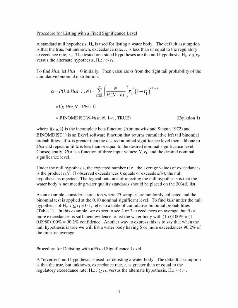
Procedure for Listing with a Fixed Significance Level A standard null hypothesis, Ho is used for listing a water body. The default assumption is that the true, but unknown, exceedance rate, r, is less than or equal to the regulatory exceedance rate, r1. The tested one-sided hypotheses are the null hypothesis, Ho: r < r1, versus the alternate hypothesis, Ha: r > r1. To find klist, let klist = 0 initially. Then calculate α from the right tail probability of the cumulative binomial distribution:

� −=

−

��

��

�

−=≥=

N

klistk

kNk

rrkNk

NNrklistkP )1( 11)!(!

!),|(

)(

1α

( )1,,1 +−Ι= klistNklistr

= BINOMDIST(N-klist, N, 1-r1, TRUE) (Equation 1)

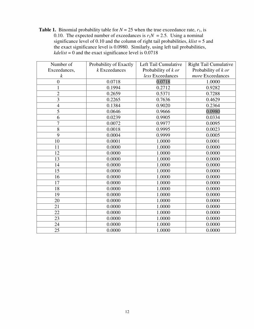
where ( )bax ,,Ι is the incomplete beta function (Abramowitz and Stegun 1972) and BINOMDIST( ) is an Excel software function that returns cumulative left tail binomial probabilities. If α is greater than the desired nominal significance level then add one to klist and repeat until α is less than or equal to the desired nominal significance level. Consequently, klist is a function of three input values: N, r1, and the desired nominal significance level. Under the null hypothesis, the expected number (i.e., the average value) of exceedances is the product r1N. If observed exceedances k equals or exceeds klist, the null hypothesis is rejected. The logical outcome of rejecting the null hypothesis is that the water body is not meeting water quality standards should be placed on the 303(d) list. As an example, consider a situation where 25 samples are randomly collected and the binomial test is applied at the 0.10 nominal significant level. To find klist under the null hypothesis of Ho: r < r1 = 0.1, refer to a table of cumulative binomial probabilities (Table 1). In this example, we expect to see 2 or 3 exceedances on average, but 5 or more exceedances is sufficient evidence to list the water body with (1-α)100% = (1-0.0980)100% = 90.2% confidence. Another way to express this is to say that when the null hypothesis is true we will list a water body having 5 or more exceedances 90.2% of the time, on average. Procedure for Delisting with a Fixed Significance Level A "reversed" null hypothesis is used for delisting a water body. The default assumption is that the true, but unknown, exceedance rate, r, is greater than or equal to the regulatory exceedance rate, Ho: r > r1, versus the alternate hypothesis, Ha: r < r1.

4

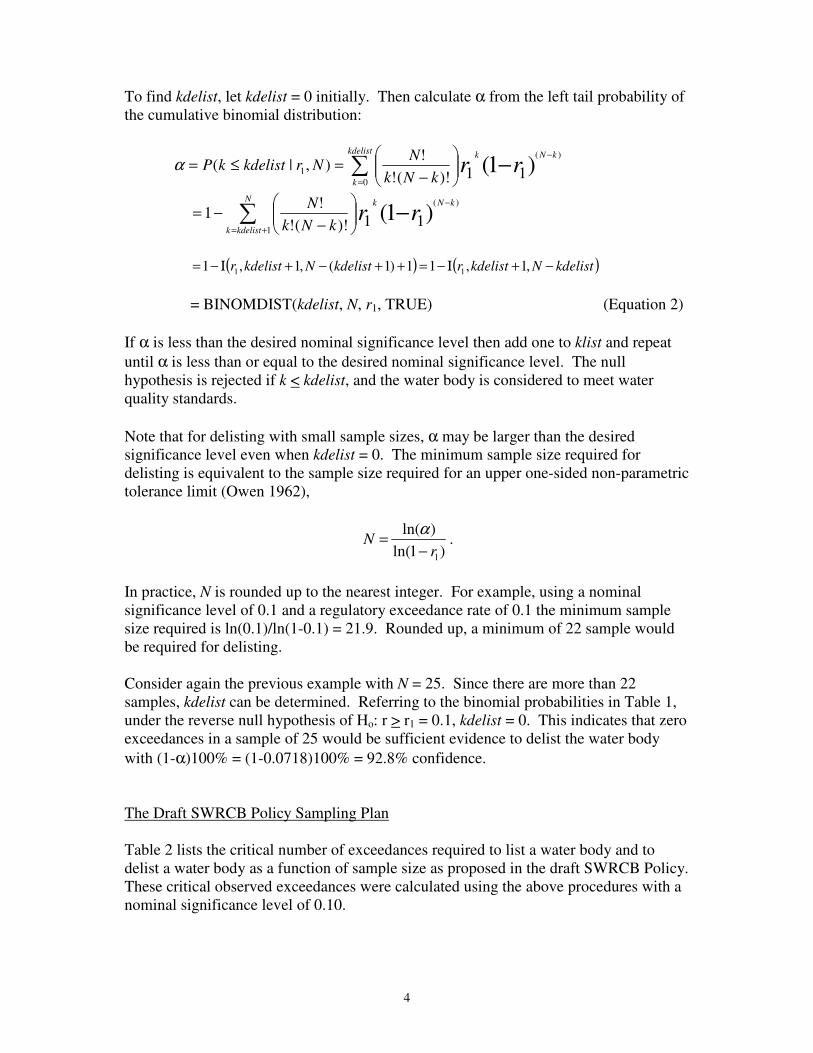
To find kdelist, let kdelist = 0 initially. Then calculate α from the left tail probability of the cumulative binomial distribution:

� −=

−

��

��

�

−=≤=

kdelist

k

kNk

rrkNk

NNrkdelistkP

0

)(

1 )1( 11)!(!!

),|(α

� −+=

−

��

��

�

−−=

N

kdelistk

kNk

rrkNk

N

1

)(

)1( 11)!(!!

1

( ) ( )kdelistNkdelistrkdelistNkdelistr −+Ι−=++−+Ι−= ,1,11)1(,1,1 11

= BINOMDIST(kdelist, N, r1, TRUE) (Equation 2)

If α is less than the desired nominal significance level then add one to klist and repeat until α is less than or equal to the desired nominal significance level. The null hypothesis is rejected if k < kdelist, and the water body is considered to meet water quality standards. Note that for delisting with small sample sizes, α may be larger than the desired significance level even when kdelist = 0. The minimum sample size required for delisting is equivalent to the sample size required for an upper one-sided non-parametric tolerance limit (Owen 1962),

)1ln()ln(

1rN

−= α

.

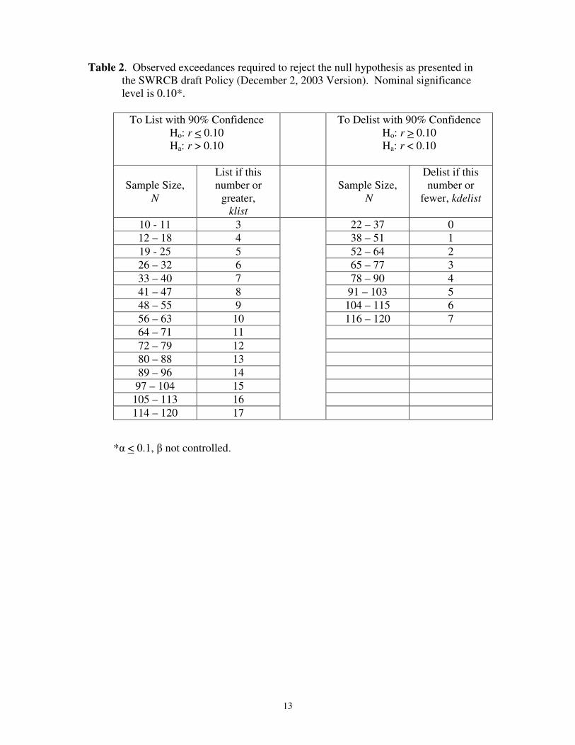
In practice, N is rounded up to the nearest integer. For example, using a nominal significance level of 0.1 and a regulatory exceedance rate of 0.1 the minimum sample size required is ln(0.1)/ln(1-0.1) = 21.9. Rounded up, a minimum of 22 sample would be required for delisting. Consider again the previous example with N = 25. Since there are more than 22 samples, kdelist can be determined. Referring to the binomial probabilities in Table 1, under the reverse null hypothesis of Ho: r > r1 = 0.1, kdelist = 0. This indicates that zero exceedances in a sample of 25 would be sufficient evidence to delist the water body with (1-α)100% = (1-0.0718)100% = 92.8% confidence. The Draft SWRCB Policy Sampling Plan Table 2 lists the critical number of exceedances required to list a water body and to delist a water body as a function of sample size as proposed in the draft SWRCB Policy. These critical observed exceedances were calculated using the above procedures with a nominal significance level of 0.10.

5

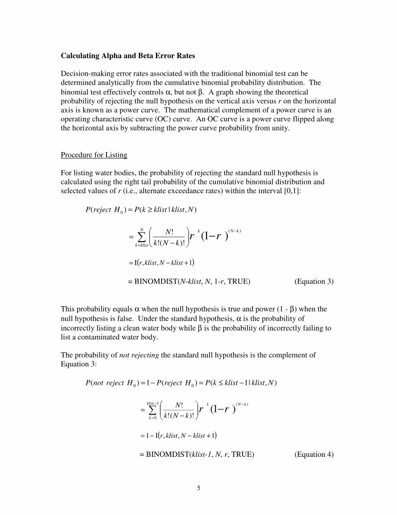
Calculating Alpha and Beta Error Rates Decision-making error rates associated with the traditional binomial test can be determined analytically from the cumulative binomial probability distribution. The binomial test effectively controls α, but not β. A graph showing the theoretical probability of rejecting the null hypothesis on the vertical axis versus r on the horizontal axis is known as a power curve. The mathematical complement of a power curve is an operating characteristic curve (OC) curve. An OC curve is a power curve flipped along the horizontal axis by subtracting the power curve probability from unity. Procedure for Listing For listing water bodies, the probability of rejecting the standard null hypothesis is calculated using the right tail probability of the cumulative binomial distribution and selected values of r (i.e., alternate exceedance rates) within the interval [0,1]:

),|()( 0 NklistklistkPHrejectP ≥=

� −=

−

��

��

�

−=

N

klistk

kNk

rrkNk

N )1( )(

)!(!!

( )1,, +−Ι= klistNklistr

= BINOMDIST(N-klist, N, 1-r, TRUE) (Equation 3)

This probability equals α when the null hypothesis is true and power (1 - β) when the null hypothesis is false. Under the standard hypothesis, α is the probability of incorrectly listing a clean water body while β is the probability of incorrectly failing to list a contaminated water body. The probability of not rejecting the standard null hypothesis is the complement of Equation 3:

),|1()(1)( 00 NklistklistkPHrejectPHrejectnotP −≤=−=

� −−

=

−

��

��

�

−=

1

0

)(

)1()!(!

!klist

k

kNk

rrkNk

N

( )1,,1 +−Ι−= klistNklistr

= BINOMDIST(klist-1, N, r, TRUE) (Equation 4)

6

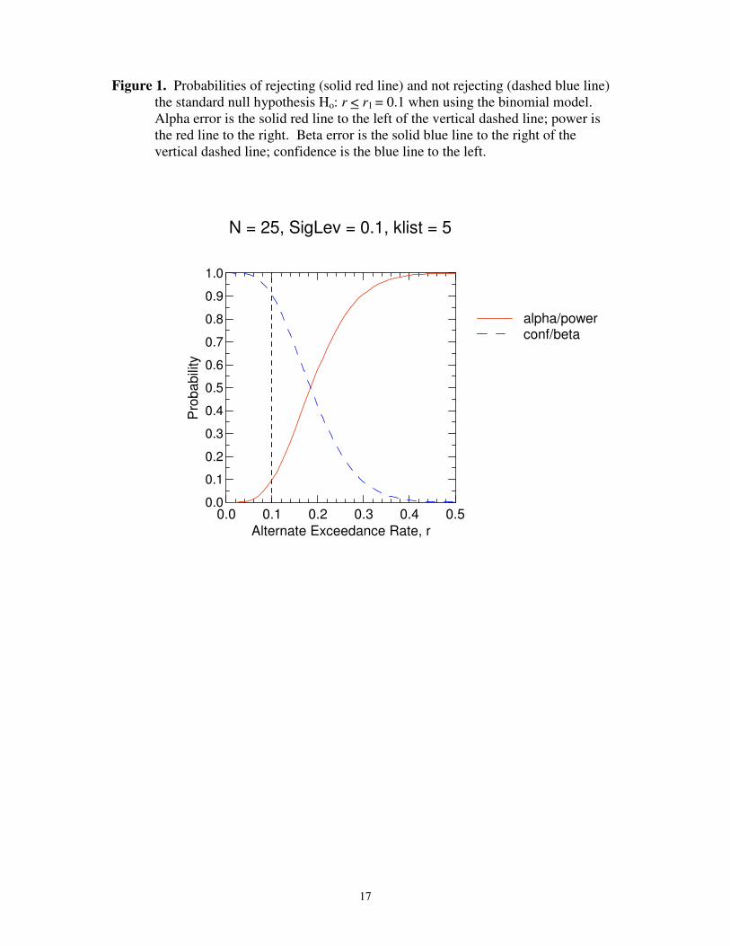
This probability equals the confidence coefficient (1-α) when the null hypothesis is true and β when the null hypothesis is false. Using the example of N = 25, Figure 1 illustrates these probabilities as a function of alternate exceedance rates for the standard null hypothesis. This graph simultaneously depicts alpha or power (via Equation 3) and confidence or beta (via Equation 4). Procedure for Delisting For delisting water bodies, the probability of rejecting the reverse null hypothesis is calculated using the left tail probability of the cumulative binomial distribution and selected values of r within the interval [0,1]:

),|()( 0 NkdelistkdelistkPHrejectP ≤=

� −=

−

��

��

�

−=

kdelist

k

kNk

rrkNk

N

0

)()1()!(!

!

( )kdelistNkdelistr −+Ι−= ,1,1

= BINOMDIST(kdelist, N, r, TRUE) (Equation 5)

Again, this probability equals α when the null hypothesis is true and power (i.e., 1 - β) when the null hypothesis is false. However, under the reverse hypothesis the nature of the errors are reversed: α is now the probability of incorrectly failing to list (delisting) a water body that doesn't meet standards while β is the probability of incorrectly listing (not delisting) a water body that does meet standards. The probability of not rejecting the reverse null hypothesis is the complement of Equation 5:

),|1()(1)( 00 NkdelistkdelistkPHrejectPHrejectnotP +≥=−=

� −+=

−

��

��

�

−=

N

kdelistk

kNk

rrkNk

N

1

)()1()!(!

!

( )kdelistNkdelistr −+Ι= ,1,

= BINOMDIST(N-kdelist-1, N, 1-r, TRUE) (Equation 6)

This probability equals the confidence coefficient (1-α) when the null hypothesis is true and β when the null hypothesis is false.

7

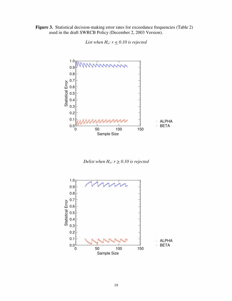
Again, using the example of N = 25, Figure 2 illustrates these probabilities as a function of alternate exceedance rates for the standard null hypothesis. Error Rates in the Draft SWRCB Policy Figures 1 and 2 show that β decreases rapidly as the true exceedance rate moves away from the hypothesized exceedance rate. In other words, the chance β of incorrectly rejecting the null hypothesis increases as the true exceedance rate gets closer to the hypothesized exceedance rate. The largest decision-making errors, therefore, are incurred when the difference between the hypothesized condition and the true condition is very small (i.e., when the effect size is very small). This can be contrasted with actual environmental effects, which continually worsen as the true exceedance rate increases toward 100%. Figure 3 shows maximal statistical error rates associated with the draft SWRCB Policy sampling plans in Table 2 for sample sizes up to 120. Notice that α is controlled at levels less than or equal to 0.10 for all sample sizes shown. The β error rate, however, is consistently greater than 0.90. In addition, larger sample sizes do not appreciably lower maximal β rates. Rates for β of 0.2 or less are generally desirable but are not achieved using this conventional hypothesis testing approach. The top graph of Figure 3 emphasizes that when deciding not to list a water body (i.e., accepting the null hypothesis of Ho: r < 0.1) we have a high probability (β > 0.90) of "missing" a water body that should, in fact, be listed. This decision error is greatest when the true alternate exceedance rate is very close to, but greater than, the hypothesized exceedance rate of r = 0.10. In contrast, the lower graph of Figure 3 emphasizes that when deciding to keep water body on the 303(d) list (i.e., accepting the null hypotheses of Ho: r > 0.1) we have a high probability (β > 0.90) of incorrectly failing to remove a water body from the 303(d) list. Again, this decision error is greatest when the true exceedance rate is very close to, but less than, the hypothesized exceedance rate of r = 0.10. Balancing Alpha and Beta Errors The binomial test, like most statistical hypothesis testing procedures, will control the maximum α rate at a value below the nominal significance level for most sample sizes. In contrast, the magnitude of β depends on several factors, including α, the population variance, the effect size, and sample size. Generally, α varies inversely with β, and control of β is traditionally sought through the appropriate selection of sample size (Gibra 1973, p.208) or through the use of a more powerful statistical test (Helsel and Hirsch 2002, p.107).

8

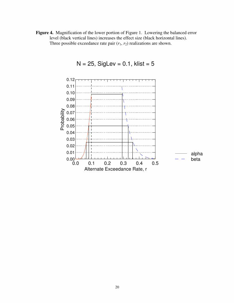
Alternatives to controlling only the α rate are possible. Mapstone (1995) argued against adhering to a fixed and arbitrary α, advocating instead for the consideration of economic, environmental, social, and political consequences of both α and β decision-making errors. In the absence of further information, Mapstone recommended that decision errors should be weighted equally, i.e., α = β. In addition, he recommended that decision-makers define a level of impact essential to detect − an effect size. Furthermore, Mapstone suggested that the effect size is perhaps the most critical aspect of environmental impact decision-making and is a biological (or chemical, physical, aesthetic, economic, etc.) decision, not simply a statistical decision. The effect size is variously called the grey region within the Data Quality Objectives (DQO) process (Millard and Neerchal 2001, p. 22) or the indifferent zone (Gibra 1973, p. 493) within the acceptance sampling process. For Clean Water Act 303(d) listing and delisting, the effect size represents the range of true exceedance rates where the consequences of decision errors are relatively minor. Riggs and Aragon (2002, Sec. D.5) applied the error balancing approach of Smith (2001) to the 303(d) listing process. To balance errors, klist and kdelist are determined in a manner different than previously described. Balanced Error Approach for Listing Figure 4 is a magnification of the lower portion of Figure 1. Examination of Figure 4 reveals that an alternate exceedance rate value r2 exists such that α = β. This can be envisioned as a horizontal line passing through the α curve and the β curve with vertical lines indicating r1 and r2. In fact, an infinite number of alternate exceedance rate pairs (r1, r2) exist that will balance α and β at a varying levels for a given N and klist. As the balanced error level decreases the effect size (r2 - r1) increases since r1 must decrease and r2 must increase. Holding r1 or r2 constant will affect the magnitude of α and β and the degree to which these errors can be balanced. The approach taken by Riggs and Aragon (2002) for listing is to first define N, r1, and r2. Next, klist is determined iteratively as the k value that minimizes the absolute difference between α and β. The minimized quantity |α - β| can be expressed using Equation 3 for α and Equation 4 for β:

|α - β| = | ( )1,,1 +−Ι klistNklistr - [ ( )1,,1 2 +−Ι− klistNklistr ] | (Equation 7)

where r1 < r2 <1. An equivalent procedure is to first define N, r1, and the effect size (r2 - r1). This minimization algorithm is analogous to the minimum squared deviation technique used in statistical curve-fitting of data. Errors will balance perfectly when the minimized quantity is zero. However, because of the discrete nature of the binomial

9

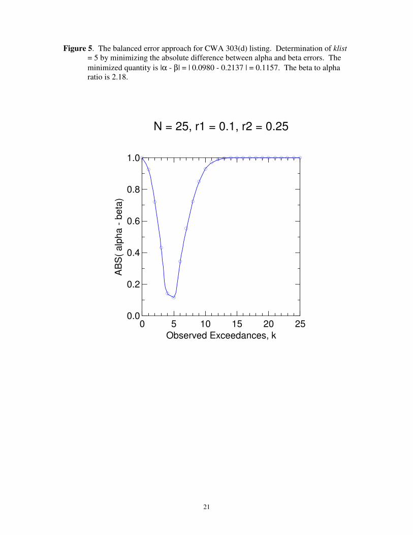
probability distribution only approximate balancing of α and β is possible, especially with smaller sample sizes. Figure 5 illustrates the determination of klist using the above balanced error approach when N = 25, r1 = 0.1, and r2 = 0.25, giving an effect size of 0.15. In this example, five observed exceedances gives the minimim absolute error difference, but the errors still cannot be balanced equitably since β is over two times larger than α. Balanced Error Approach for Delisting For delisting, the Riggs and Aragon (2002) approach is to again define N, r1, and r2, but this time r2 is a value less than r1. kdelist is determined as the k value that minimizes the absolute difference between α and β. The minimized quantity |α - β| can be expressed using Equation 5 for α and Equation 6 for β:

|α - β| = | [ ( )kdelistNkdelistr −+Ι− ,1,1 1 ] - ( )kdelistNkdelistr −+Ι ,1,2 | (Equation 8)

where r2 < r1 <1. SWRCB staff developed a computer program, BinomBal.exe, that will evaluate the minimized quantities in Equations 7 or 9 to derive klist or kdelist. Choosing Appropriate Starting Values with the Balanced Error Approach An important consideration when calculating klist and kdelist by the balanced error approach is the values assigned to r1 and r2 for both listing and delisting. It is possible, and undesirable, to assign r1 and r2 values that would result in conflicting decision rules for listing and delisting. Under such starting values, a set of observed exceedances will exist that simultaneously result in a decision to list under the standard null hypothesis and a decision to delist under the reverse null hypothesis for a given N. For example, given N = 25 and for listing r1 = 0.10 and r2 = 0.25, but for delisting r1 = 0.40 and r2 = 0.25. Using the balanced error approach leads to klist = 5 or more exceedances and kdelist = 6 or less exceedances. A water body listed with 5 or 6 exceedances in a sample of 25 could then immediately be delisted! Generally, the balanced error approach should result in a kdelist value that is at least one exceedance less than klist. A special case exists when r1 (listing) = r2 (delisting) and r2 (listing) = r1 (delisting). This special case of r1 and r2 starting values results in the equality of the minimized error quantities in Equations 7 and 8. Equating these equations means that kdelist will always be one less than klist. Thus, α for listing becomes exactly equal to β for delisting and vise-versa. This reversal and equality of errors for listing and delisting is desirable because conflicting decisions based on which null hypothesis is chosen (standard versus reversed) will then be eliminated. Indeed, Smith (2001) noted that

10

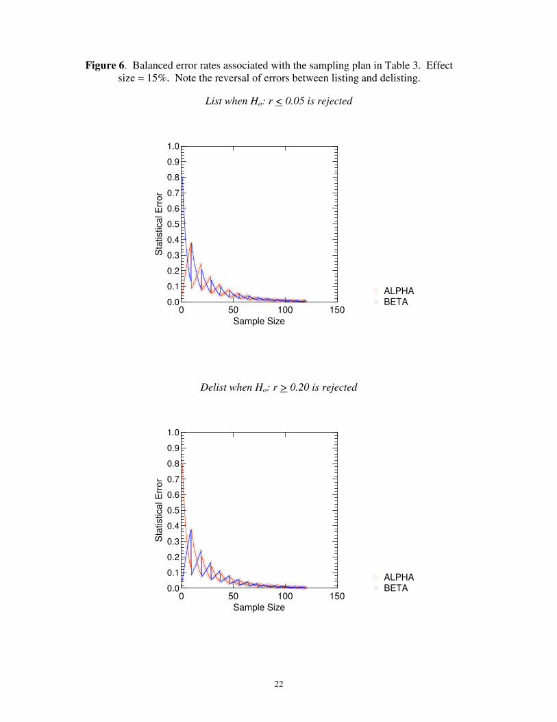
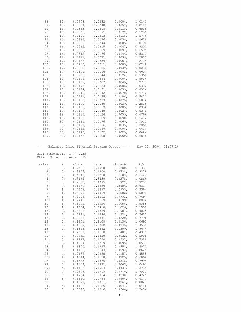
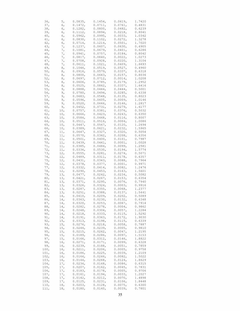
balanced decision error rates are less affected by switching the null and alternative hypothesis. Comparison of the Draft SWRCB Policy with the Balanced Error Approach The balanced error approach is useful because it considers both types of decision-making errors, α and β, rather than only α when designing sampling plans. Another objective is to maintain these balanced error rates at or below an acceptable magnitude. Although Riggs and Aragon (2002) suggested that a moderate acceptable magnitude for balancing errors is 15%, the choice of values for α and β rates is a subjective policy decision (Millard and Neerchal 2001). Nevertheless, a pre-defined maximum acceptable error for both α and β will allow the determination of acceptable sample sizes to use for listing and delisting. Tables 3-5 list selected sampling plans and the critical number of exceedances required to list or delist a water body as a function of sample size when applying the balanced error approach with no conflicting decision rules. More detailed output from the BinomBal program for these selected sampling plans is included in the Appendix. Figures 6-8 display statistical error rates associated with the sampling plans of Tables 3-5. Notice that by using the balanced error approach both α and β decrease appreciably with increasing N. Lowered α and β rates using the balanced error approach contrast sharply with the higher β error rates expected when using the traditional binomial test. Figure 9 directly compares the selected balanced error sampling plans with the existing SWRCB Policy sampling plans. With small sample sizes under 60 the balanced error plans require fewer exceedances to list a water body and allow more exceedances when delisting a water body. Appropriate sample sizes required to achieve desired error rates can be read from Figures 6-8. If the effect size is 15% (Figures 6 and 8) and we wish to maintain both α and β rates at or below 0.15 then about 30 samples are needed. To maintain both α and β rates at or below 0.20 about 20 samples are needed. A 10% effect size (Figure 7) results in more rigorous sample size requirements. To maintain both α and β rates at or below 0.15 about 65 samples are needed. To maintain both α and β rates at or below 0.20 about 50 samples are needed. In conclusion, the error balancing approach is an equitable way to decide whether a water body should be listed or delisted − as long as a sufficient number of samples are collected to keep the error rates below at moderate levels of 15-20%.

11

References: Abramowitz, M. and I. A. Stegun (eds). 1972. Handbook of mathematical functions,

10th printing. Dover Publications, Inc. NY. Gibra, I. N. 1973. Probability and statistical inference for scientists and engineers.

Prentice-Hall, Inc. NJ. Helsel, D. R. and R. M. Hirsch. 2002. Statistical methods in water resources. Chapter

A3. Techniques of water-resources investigations of the United States Geological Survey, Book 4, Hydrologic analysis and interpretation. http://water.usgs.gov/pubs/twri/twri4a3/

Mapstone, B. D. 1995. Scalable decision rules for environmental impact studies:

Effect size, Type I, and Type II Errors. Ecological Applications 5(2):401-410 Millard, S. P. and N. K. Neerchal. 2001. Environmental Statistics with S-Plus. CRC

Press, NY. Owen, D. B. 1962. Handbook of statistical tables. Section 10.1. Addison-Westley Inc.,

Reading MA. Riggs, M. and E. Aragon. 2002. Interval estimators and hypothesis tests for data

quality assessments in water quality attainment studies (Draft). Appendix D in USEPA, 2002, Consolidated Assessment and Listing Methodology: Toward a compendium of best management practices. Office of Wetlands Oceans and Watersheds. http://www.epa.gov/owow/monitoring/calm/calm_contents.pdf

Smith, E. P., K. Ye, C. Hughes, and L. Shabman. 2001. Statistical assessment of

violations of water quality standards under Section 303(d) of the Clean Water Act. Environ. Sci. Technol. 35:606-612.

SWRCB. 2003. Water Quality Control Policy for developing California's Clean Water

Act Section 303(d) list. Draft Functional Equivalent Document, December 2003.

12

Table 1. Binomial probability table for N = 25 when the true exceedance rate, r1, is 0.10. The expected number of exceedances is r1N = 2.5. Using a nominal significance level of 0.10 and the column of right tail probabilities, klist = 5 and the exact significance level is 0.0980. Similarly, using left tail probabilities, kdelist = 0 and the exact significance level is 0.0718

Number of

Exceedances, k

Probability of Exactly k Exceedances

Left Tail Cumulative Probability of k or less Exceedances

Right Tail Cumulative Probability of k or more Exceedances

0 0.0718 0.0718 1.0000 1 0.1994 0.2712 0.9282 2 0.2659 0.5371 0.7288 3 0.2265 0.7636 0.4629 4 0.1384 0.9020 0.2364 5 0.0646 0.9666 0.0980 6 0.0239 0.9905 0.0334 7 0.0072 0.9977 0.0095 8 0.0018 0.9995 0.0023 9 0.0004 0.9999 0.0005

10 0.0001 1.0000 0.0001 11 0.0000 1.0000 0.0000 12 0.0000 1.0000 0.0000 13 0.0000 1.0000 0.0000 14 0.0000 1.0000 0.0000 15 0.0000 1.0000 0.0000 16 0.0000 1.0000 0.0000 17 0.0000 1.0000 0.0000 18 0.0000 1.0000 0.0000 19 0.0000 1.0000 0.0000 20 0.0000 1.0000 0.0000 21 0.0000 1.0000 0.0000 22 0.0000 1.0000 0.0000 23 0.0000 1.0000 0.0000 24 0.0000 1.0000 0.0000 25 0.0000 1.0000 0.0000

13

Table 2. Observed exceedances required to reject the null hypothesis as presented in the SWRCB draft Policy (December 2, 2003 Version). Nominal significance level is 0.10*.

To List with 90% Confidence

Ho: r < 0.10 Ha: r > 0.10

To Delist with 90% Confidence Ho: r > 0.10 Ha: r < 0.10

Sample Size, N

List if this number or

greater, klist

Sample Size,

N

Delist if this number or

fewer, kdelist

10 - 11 3 22 – 37 0 12 – 18 4 38 – 51 1 19 - 25 5 52 – 64 2 26 – 32 6 65 – 77 3 33 – 40 7 78 – 90 4 41 – 47 8 91 – 103 5 48 – 55 9 104 – 115 6 56 – 63 10 116 – 120 7 64 – 71 11 72 – 79 12 80 – 88 13 89 – 96 14

97 – 104 15 105 – 113 16 114 – 120 17

*� < 0.1, � not controlled.

14

Table 3. Observed exceedances required to reject the null hypothesis based on the

balanced error approach. Effect size = 15%.

List Sample Plan Ho: r < 0.05 Ha: r > 0.20

Delist Sample Plan Ho: r > 0.20 Ha: r < 0.05

Sample Size,

N


greater, klist

Sample Size,

N


fewer, kdelist

1 – 9 1 1 – 9 0 10 – 19 2 10 – 19 1

20 (21)*– 28 3 20 (21)*– 28 2 29** – 37 4 29** – 37 3

38 – 46 5 38 – 46 4 47 – 55 6 47 – 55 5 56 – 64 7 56 – 64 6 65 – 73 8 65 – 73 7 74 – 82 9 74 – 82 8 83 – 91 10 83 – 91 9

92 – 100 11 92 – 100 10 101 – 109 12 101 – 109 11 110 – 118 13 110 – 118 12 119 – 120 14

119 – 120 13 * � and � < 0.2 at Sample Size = 21. ** � and � < 0.15 at Sample Size = 29

15

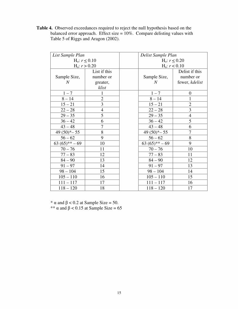
Table 4. Observed exceedances required to reject the null hypothesis based on the balanced error approach. Effect size = 10%. Compare delisting values with Table 5 of Riggs and Aragon (2002).

List Sample Plan Ho: r < 0.10 Ha: r > 0.20

Delist Sample Plan Ho: r < 0.20 Ha: r < 0.10

Sample Size,

N


greater, klist

Sample Size,

N


fewer, kdelist

1 – 7 1 1 – 7 0 8 – 14 2 8 – 14 1

15 – 21 3 15 – 21 2 22 – 28 4 22 – 28 3 29 – 35 5 29 – 35 4 36 – 42 6 36 – 42 5 43 – 48 7 43 – 48 6

49 (50)*– 55 8 49 (50)*– 55 7 56 – 62 9 56 – 62 8

63 (65)** – 69 10 63 (65)** – 69 9 70 – 76 11 70 – 76 10 77 – 83 12 77 – 83 11 84 – 90 13 84 – 90 12 91 – 97 14 91 – 97 13

98 – 104 15 98 – 104 14 105 – 110 16 105 – 110 15 111 – 117 17 111 – 117 16 118 – 120 18

118 – 120 17 * � and � < 0.2 at Sample Size = 50. ** � and � < 0.15 at Sample Size = 65

16

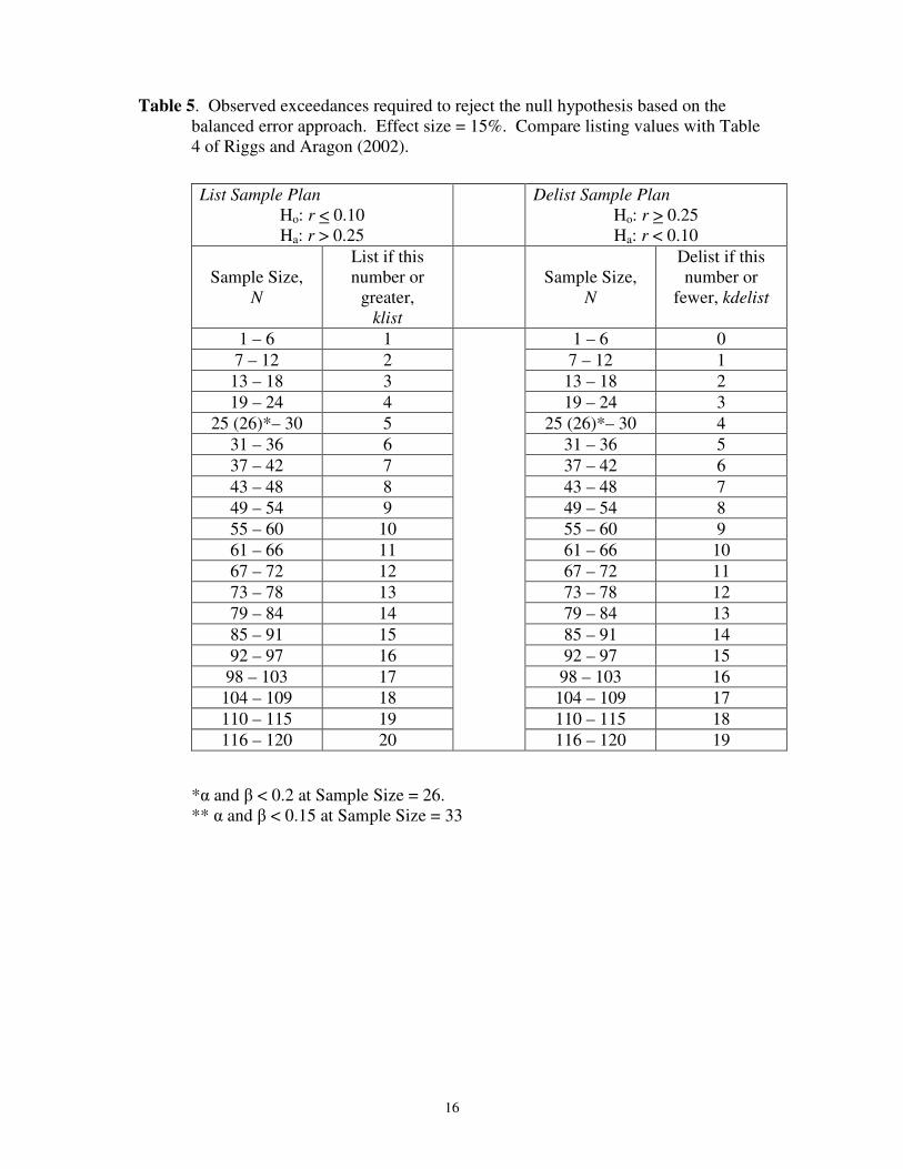
Table 5. Observed exceedances required to reject the null hypothesis based on the balanced error approach. Effect size = 15%. Compare listing values with Table 4 of Riggs and Aragon (2002).

List Sample Plan

Ho: r < 0.10 Ha: r > 0.25

Delist Sample Plan Ho: r > 0.25 Ha: r < 0.10

Sample Size,

N


greater, klist

Sample Size,

N


fewer, kdelist

1 – 6 1 1 – 6 0 7 – 12 2 7 – 12 1

13 – 18 3 13 – 18 2 19 – 24 4 19 – 24 3

25 (26)*– 30 5 25 (26)*– 30 4 31 – 36 6 31 – 36 5 37 – 42 7 37 – 42 6 43 – 48 8 43 – 48 7 49 – 54 9 49 – 54 8 55 – 60 10 55 – 60 9 61 – 66 11 61 – 66 10 67 – 72 12 67 – 72 11 73 – 78 13 73 – 78 12 79 – 84 14 79 – 84 13 85 – 91 15 85 – 91 14 92 – 97 16 92 – 97 15

98 – 103 17 98 – 103 16 104 – 109 18 104 – 109 17 110 – 115 19 110 – 115 18 116 – 120 20

116 – 120 19 *� and � < 0.2 at Sample Size = 26. ** � and � < 0.15 at Sample Size = 33

17

Figure 1. Probabilities of rejecting (solid red line) and not rejecting (dashed blue line) the standard null hypothesis Ho: r < r1 = 0.1 when using the binomial model. Alpha error is the solid red line to the left of the vertical dashed line; power is the red line to the right. Beta error is the solid blue line to the right of the vertical dashed line; confidence is the blue line to the left.

N = 25, SigLev = 0.1, klist = 5

0.0 0.1 0.2 0.3 0.4 0.5Alternate Exceedance Rate, r

0.0

0.1

0.2

0.3

0.4

0.5

0.6

0.7

0.8

0.9

1.0

Pro

babi

lity

conf/betaalpha/power

18

Figure 2. Probabilities of rejecting (solid red line) and not rejecting (blue line) the reverse null hypothesis Ho: r > r1 = 0.1 when using the binomial model. Alpha error is the solid red line to the right of the vertical dashed line; power is the red line to the left. Beta error is the dashed blue line to the left of the vertical dashed line; confidence is the blue line to the right.

N = 25, SigLev = 0.1, kdelist = 0


0.0

0.1

0.2

0.3

0.4

0.5

0.6

0.7

0.8

0.9

1.0

Pro

babi

lity

beta / confpower / alpha

19

Figure 3. Statistical decision-making error rates for exceedance frequencies (Table 2) used in the draft SWRCB Policy (December 2, 2003 Version).

List when Ho: r < 0.10 is rejected

0 50 100 150Sample Size

0.0

0.1

0.2

0.3

0.4

0.5

0.6

0.7

0.8

0.9

1.0S

tatis

tical

Err

or

BETAALPHA

Delist when Ho: r > 0.10 is rejected


0.0

0.1

0.2

0.3

0.4

0.5

0.6

0.7

0.8

0.9

1.0

Sta

tistic

al E

rror

BETAALPHA

20

Figure 4. Magnification of the lower portion of Figure 1. Lowering the balanced error

level (black vertical lines) increases the effect size (black horizontal lines). Three possible exceedance rate pair (r1, r2) realizations are shown.

N = 25, SigLev = 0.1, klist = 5


0.00

0.01

0.02

0.03

0.04

0.05

0.06

0.07

0.08

0.09

0.10

0.11

0.12

Pro

babi

lity

betaalpha

21

Figure 5. The balanced error approach for CWA 303(d) listing. Determination of klist = 5 by minimizing the absolute difference between alpha and beta errors. The minimized quantity is |α - β| = | 0.0980 - 0.2137 | = 0.1157. The beta to alpha ratio is 2.18.

N = 25, r1 = 0.1, r2 = 0.25

0 5 10 15 20 25Observed Exceedances, k

0.0

0.2

0.4

0.6

0.8

1.0

AB

S( a

lpha

- be

ta)

22

Figure 6. Balanced error rates associated with the sampling plan in Table 3. Effect size = 15%. Note the reversal of errors between listing and delisting.



0.0

0.1

0.2

0.3

0.4

0.5

0.6

0.7

0.8

0.9

1.0S

tatis

tical

Err

or

BETAALPHA



0.0

0.1

0.2

0.3

0.4

0.5

0.6

0.7

0.8

0.9

1.0

Sta

tistic

al E

rror

BETAALPHA

23

Figure 7. Balanced error rates associated with the sampling plan in Table 4. Effect size = 10%. Note the reversal of errors between listing and delisting.

List Ho: r < 0.10 is rejected


0.0

0.1

0.2

0.3

0.4

0.5

0.6

0.7

0.8

0.9

1.0S

tatis

tical

Err

or

BETAALPHA



0.0

0.1

0.2

0.3

0.4

0.5

0.6

0.7

0.8

0.9

1.0

Sta

tistic

al E

rror

BETAALPHA

24

Figure 8. Balanced error rates associated with the sampling plan in Table 5. Effect

size = 15%. Note the reversal of errors between listing and delisting.



0.0

0.1

0.2

0.3

0.4

0.5

0.6

0.7

0.8

0.9

1.0S

tatis

tical

Err

or

BETAALPHA



0.0

0.1

0.2

0.3

0.4

0.5

0.6

0.7

0.8

0.9

1.0

Sta

tistic

al E

rror

BETAALPHA

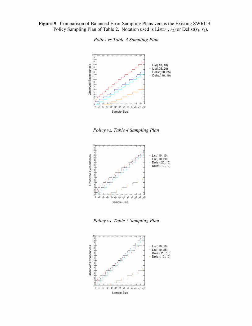
Figure 9. Comparison of Balanced Error Sampling Plans versus the Existing SWRCB Policy Sampling Plan of Table 2. Notation used is List(r1, r2) or Delist(r1, r2).

Policy vs.Table 3 Sampling Plan

0 10 20 30 40 50 60 70 80 90100

110120

Sample Size

0123456789

1011121314151617181920

Obs

erve

d E

xcee

danc

es

Delist(.10,.10)Delist(.20,.05)List(.05,.20)List(.10,.10)

Policy vs. Table 4 Sampling Plan

0 10 20 30 40 50 60 70 80 90100

110120

Sample Size

0123456789

1011121314151617181920

Obs

erve

d E

xcee

danc

es


Policy vs. Table 5 Sampling Plan

0 10 20 30 40 50 60 70 80 90100

110120

Sample Size

0123456789

1011121314151617181920

Obs

erve

d E

xcee

danc

es


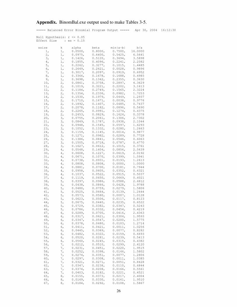
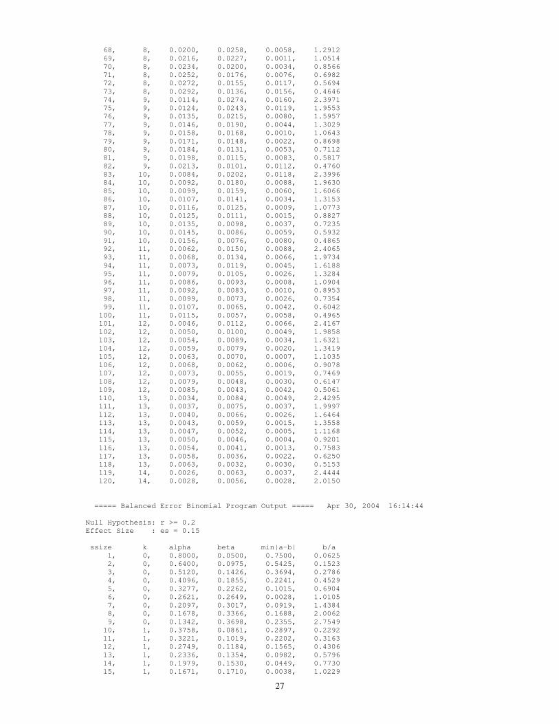
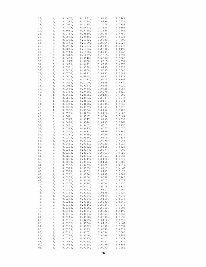
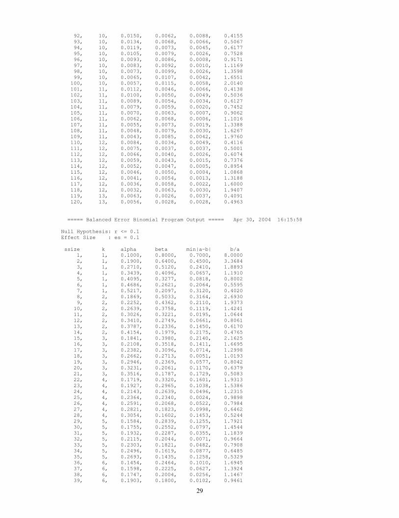
26

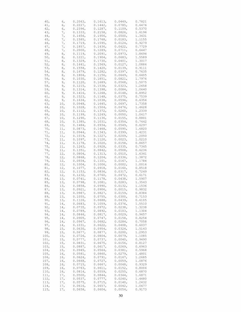
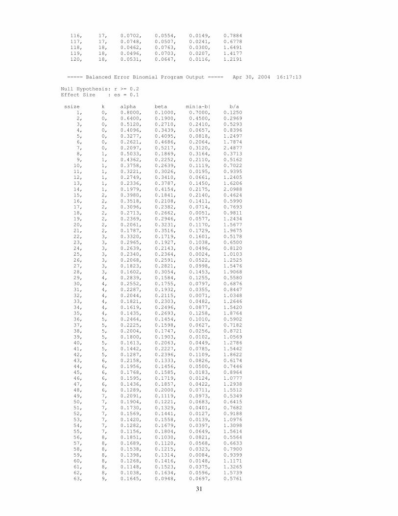
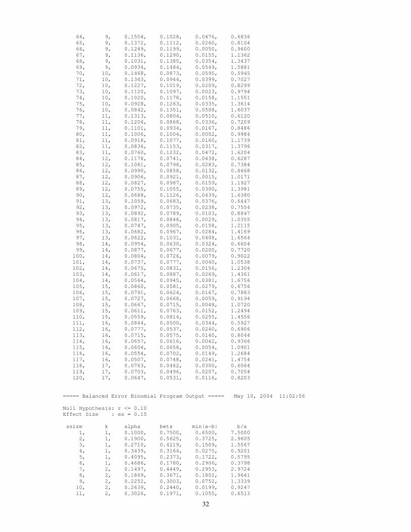
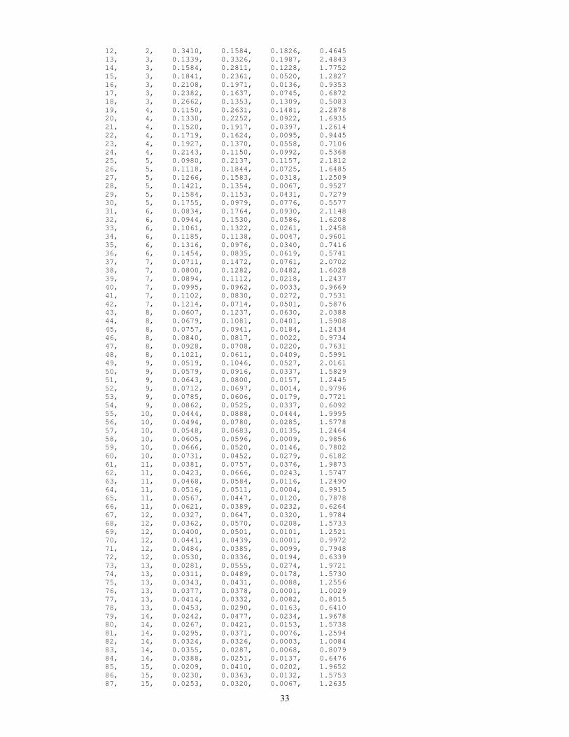
Appendix. BinomBal.exe output used to make Tables 3-5. ===== Balanced Error Binomial Program Output ===== Apr 30, 2004 16:12:30 Null Hypothesis: r <= 0.05 Effect Size : es = 0.15 ssize k alpha beta min|a-b| b/a 1, 1, 0.0500, 0.8000, 0.7500, 16.0000 2, 1, 0.0975, 0.6400, 0.5425, 6.5641 3, 1, 0.1426, 0.5120, 0.3694, 3.5898 4, 1, 0.1855, 0.4096, 0.2241, 2.2082 5, 1, 0.2262, 0.3277, 0.1015, 1.4485 6, 1, 0.2649, 0.2621, 0.0028, 0.9896 7, 1, 0.3017, 0.2097, 0.0919, 0.6952 8, 1, 0.3366, 0.1678, 0.1688, 0.4985 9, 1, 0.3698, 0.1342, 0.2355, 0.3630 10, 2, 0.0861, 0.3758, 0.2897, 4.3629 11, 2, 0.1019, 0.3221, 0.2202, 3.1613 12, 2, 0.1184, 0.2749, 0.1565, 2.3224 13, 2, 0.1354, 0.2336, 0.0982, 1.7253 14, 2, 0.1530, 0.1979, 0.0449, 1.2937 15, 2, 0.1710, 0.1671, 0.0038, 0.9776 16, 2, 0.1892, 0.1407, 0.0485, 0.7437 17, 2, 0.2078, 0.1182, 0.0896, 0.5690 18, 2, 0.2265, 0.0991, 0.1274, 0.4375 19, 2, 0.2453, 0.0829, 0.1624, 0.3378 20, 3, 0.0755, 0.2061, 0.1306, 2.7302 21, 3, 0.0849, 0.1787, 0.0938, 2.1044 22, 3, 0.0948, 0.1545, 0.0597, 1.6293 23, 3, 0.1052, 0.1332, 0.0280, 1.2663 24, 3, 0.1159, 0.1145, 0.0014, 0.9877 25, 3, 0.1271, 0.0982, 0.0289, 0.7728 26, 3, 0.1386, 0.0841, 0.0546, 0.6063 27, 3, 0.1505, 0.0718, 0.0787, 0.4770 28, 3, 0.1627, 0.0612, 0.1015, 0.3761 29, 4, 0.0548, 0.1404, 0.0856, 2.5639 30, 4, 0.0608, 0.1227, 0.0619, 2.0192 31, 4, 0.0671, 0.1070, 0.0399, 1.5941 32, 4, 0.0738, 0.0931, 0.0193, 1.2613 33, 4, 0.0808, 0.0808, 0.0000, 1.0000 34, 4, 0.0881, 0.0700, 0.0181, 0.7944 35, 4, 0.0958, 0.0605, 0.0352, 0.6321 36, 4, 0.1037, 0.0522, 0.0515, 0.5037 37, 4, 0.1119, 0.0450, 0.0669, 0.4021 38, 5, 0.0397, 0.0986, 0.0588, 2.4812 39, 5, 0.0438, 0.0866, 0.0428, 1.9788 40, 5, 0.0480, 0.0759, 0.0279, 1.5806 41, 5, 0.0525, 0.0664, 0.0139, 1.2644 42, 5, 0.0573, 0.0580, 0.0007, 1.0128 43, 5, 0.0623, 0.0506, 0.0117, 0.8123 44, 5, 0.0675, 0.0440, 0.0235, 0.6522 45, 5, 0.0729, 0.0382, 0.0347, 0.5243 46, 5, 0.0786, 0.0332, 0.0454, 0.4219 47, 6, 0.0289, 0.0705, 0.0416, 2.4363 48, 6, 0.0317, 0.0621, 0.0304, 1.9593 49, 6, 0.0347, 0.0547, 0.0200, 1.5775 50, 6, 0.0378, 0.0480, 0.0103, 1.2714 51, 6, 0.0411, 0.0421, 0.0011, 1.0256 52, 6, 0.0445, 0.0369, 0.0077, 0.8282 53, 6, 0.0482, 0.0322, 0.0159, 0.6693 54, 6, 0.0520, 0.0281, 0.0239, 0.5413 55, 6, 0.0560, 0.0245, 0.0315, 0.4382 56, 7, 0.0212, 0.0510, 0.0299, 2.4120 57, 7, 0.0231, 0.0451, 0.0220, 1.9515 58, 7, 0.0252, 0.0398, 0.0146, 1.5802 59, 7, 0.0274, 0.0351, 0.0077, 1.2806 60, 7, 0.0297, 0.0308, 0.0011, 1.0385 61, 7, 0.0321, 0.0271, 0.0051, 0.8428 62, 7, 0.0347, 0.0238, 0.0110, 0.6844 63, 7, 0.0374, 0.0208, 0.0166, 0.5561 64, 7, 0.0403, 0.0182, 0.0221, 0.4521 65, 8, 0.0155, 0.0373, 0.0217, 2.4004 66, 8, 0.0169, 0.0330, 0.0161, 1.9510 67, 8, 0.0184, 0.0292, 0.0108, 1.5867

27

68, 8, 0.0200, 0.0258, 0.0058, 1.2912 69, 8, 0.0216, 0.0227, 0.0011, 1.0514 70, 8, 0.0234, 0.0200, 0.0034, 0.8566 71, 8, 0.0252, 0.0176, 0.0076, 0.6982 72, 8, 0.0272, 0.0155, 0.0117, 0.5694 73, 8, 0.0292, 0.0136, 0.0156, 0.4646 74, 9, 0.0114, 0.0274, 0.0160, 2.3971 75, 9, 0.0124, 0.0243, 0.0119, 1.9553 76, 9, 0.0135, 0.0215, 0.0080, 1.5957 77, 9, 0.0146, 0.0190, 0.0044, 1.3029 78, 9, 0.0158, 0.0168, 0.0010, 1.0643 79, 9, 0.0171, 0.0148, 0.0022, 0.8698 80, 9, 0.0184, 0.0131, 0.0053, 0.7112 81, 9, 0.0198, 0.0115, 0.0083, 0.5817 82, 9, 0.0213, 0.0101, 0.0112, 0.4760 83, 10, 0.0084, 0.0202, 0.0118, 2.3996 84, 10, 0.0092, 0.0180, 0.0088, 1.9630 85, 10, 0.0099, 0.0159, 0.0060, 1.6066 86, 10, 0.0107, 0.0141, 0.0034, 1.3153 87, 10, 0.0116, 0.0125, 0.0009, 1.0773 88, 10, 0.0125, 0.0111, 0.0015, 0.8827 89, 10, 0.0135, 0.0098, 0.0037, 0.7235 90, 10, 0.0145, 0.0086, 0.0059, 0.5932 91, 10, 0.0156, 0.0076, 0.0080, 0.4865 92, 11, 0.0062, 0.0150, 0.0088, 2.4065 93, 11, 0.0068, 0.0134, 0.0066, 1.9734 94, 11, 0.0073, 0.0119, 0.0045, 1.6188 95, 11, 0.0079, 0.0105, 0.0026, 1.3284 96, 11, 0.0086, 0.0093, 0.0008, 1.0904 97, 11, 0.0092, 0.0083, 0.0010, 0.8953 98, 11, 0.0099, 0.0073, 0.0026, 0.7354 99, 11, 0.0107, 0.0065, 0.0042, 0.6042 100, 11, 0.0115, 0.0057, 0.0058, 0.4965 101, 12, 0.0046, 0.0112, 0.0066, 2.4167 102, 12, 0.0050, 0.0100, 0.0049, 1.9858 103, 12, 0.0054, 0.0089, 0.0034, 1.6321 104, 12, 0.0059, 0.0079, 0.0020, 1.3419 105, 12, 0.0063, 0.0070, 0.0007, 1.1035 106, 12, 0.0068, 0.0062, 0.0006, 0.9078 107, 12, 0.0073, 0.0055, 0.0019, 0.7469 108, 12, 0.0079, 0.0048, 0.0030, 0.6147 109, 12, 0.0085, 0.0043, 0.0042, 0.5061 110, 13, 0.0034, 0.0084, 0.0049, 2.4295 111, 13, 0.0037, 0.0075, 0.0037, 1.9997 112, 13, 0.0040, 0.0066, 0.0026, 1.6464 113, 13, 0.0043, 0.0059, 0.0015, 1.3558 114, 13, 0.0047, 0.0052, 0.0005, 1.1168 115, 13, 0.0050, 0.0046, 0.0004, 0.9201 116, 13, 0.0054, 0.0041, 0.0013, 0.7583 117, 13, 0.0058, 0.0036, 0.0022, 0.6250 118, 13, 0.0063, 0.0032, 0.0030, 0.5153 119, 14, 0.0026, 0.0063, 0.0037, 2.4444 120, 14, 0.0028, 0.0056, 0.0028, 2.0150 ===== Balanced Error Binomial Program Output ===== Apr 30, 2004 16:14:44 Null Hypothesis: r >= 0.2 Effect Size : es = 0.15 ssize k alpha beta min|a-b| b/a 1, 0, 0.8000, 0.0500, 0.7500, 0.0625 2, 0, 0.6400, 0.0975, 0.5425, 0.1523 3, 0, 0.5120, 0.1426, 0.3694, 0.2786 4, 0, 0.4096, 0.1855, 0.2241, 0.4529 5, 0, 0.3277, 0.2262, 0.1015, 0.6904 6, 0, 0.2621, 0.2649, 0.0028, 1.0105 7, 0, 0.2097, 0.3017, 0.0919, 1.4384 8, 0, 0.1678, 0.3366, 0.1688, 2.0062 9, 0, 0.1342, 0.3698, 0.2355, 2.7549 10, 1, 0.3758, 0.0861, 0.2897, 0.2292 11, 1, 0.3221, 0.1019, 0.2202, 0.3163 12, 1, 0.2749, 0.1184, 0.1565, 0.4306 13, 1, 0.2336, 0.1354, 0.0982, 0.5796 14, 1, 0.1979, 0.1530, 0.0449, 0.7730 15, 1, 0.1671, 0.1710, 0.0038, 1.0229

28

16, 1, 0.1407, 0.1892, 0.0485, 1.3446 17, 1, 0.1182, 0.2078, 0.0896, 1.7575 18, 1, 0.0991, 0.2265, 0.1274, 2.2858 19, 1, 0.0829, 0.2453, 0.1624, 2.9601 20, 2, 0.2061, 0.0755, 0.1306, 0.3663 21, 2, 0.1787, 0.0849, 0.0938, 0.4752 22, 2, 0.1545, 0.0948, 0.0597, 0.6138 23, 2, 0.1332, 0.1052, 0.0280, 0.7897 24, 2, 0.1145, 0.1159, 0.0014, 1.0125 25, 2, 0.0982, 0.1271, 0.0289, 1.2940 26, 2, 0.0841, 0.1386, 0.0546, 1.6492 27, 2, 0.0718, 0.1505, 0.0787, 2.0966 28, 2, 0.0612, 0.1627, 0.1015, 2.6592 29, 3, 0.1404, 0.0548, 0.0856, 0.3900 30, 3, 0.1227, 0.0608, 0.0619, 0.4952 31, 3, 0.1070, 0.0671, 0.0399, 0.6273 32, 3, 0.0931, 0.0738, 0.0193, 0.7928 33, 3, 0.0808, 0.0808, 0.0000, 1.0000 34, 3, 0.0700, 0.0881, 0.0181, 1.2589 35, 3, 0.0605, 0.0958, 0.0352, 1.5821 36, 3, 0.0522, 0.1037, 0.0515, 1.9851 37, 3, 0.0450, 0.1119, 0.0669, 2.4872 38, 4, 0.0986, 0.0397, 0.0588, 0.4030 39, 4, 0.0866, 0.0438, 0.0428, 0.5054 40, 4, 0.0759, 0.0480, 0.0279, 0.6327 41, 4, 0.0664, 0.0525, 0.0139, 0.7909 42, 4, 0.0580, 0.0573, 0.0007, 0.9874 43, 4, 0.0506, 0.0623, 0.0117, 1.2311 44, 4, 0.0440, 0.0675, 0.0235, 1.5332 45, 4, 0.0382, 0.0729, 0.0347, 1.9073 46, 4, 0.0332, 0.0786, 0.0454, 2.3703 47, 5, 0.0705, 0.0289, 0.0416, 0.4105 48, 5, 0.0621, 0.0317, 0.0304, 0.5104 49, 5, 0.0547, 0.0347, 0.0200, 0.6339 50, 5, 0.0480, 0.0378, 0.0103, 0.7866 51, 5, 0.0421, 0.0411, 0.0011, 0.9750 52, 5, 0.0369, 0.0445, 0.0077, 1.2075 53, 5, 0.0322, 0.0482, 0.0159, 1.4942 54, 5, 0.0281, 0.0520, 0.0239, 1.8474 55, 5, 0.0245, 0.0560, 0.0315, 2.2823 56, 6, 0.0510, 0.0212, 0.0299, 0.4146 57, 6, 0.0451, 0.0231, 0.0220, 0.5124 58, 6, 0.0398, 0.0252, 0.0146, 0.6328 59, 6, 0.0351, 0.0274, 0.0077, 0.7809 60, 6, 0.0308, 0.0297, 0.0011, 0.9629 61, 6, 0.0271, 0.0321, 0.0051, 1.1866 62, 6, 0.0238, 0.0347, 0.0110, 1.4612 63, 6, 0.0208, 0.0374, 0.0166, 1.7982 64, 6, 0.0182, 0.0403, 0.0221, 2.2117 65, 7, 0.0373, 0.0155, 0.0217, 0.4166 66, 7, 0.0330, 0.0169, 0.0161, 0.5126 67, 7, 0.0292, 0.0184, 0.0108, 0.6302 68, 7, 0.0258, 0.0200, 0.0058, 0.7745 69, 7, 0.0227, 0.0216, 0.0011, 0.9511 70, 7, 0.0200, 0.0234, 0.0034, 1.1675 71, 7, 0.0176, 0.0252, 0.0076, 1.4322 72, 7, 0.0155, 0.0272, 0.0117, 1.7562 73, 7, 0.0136, 0.0292, 0.0156, 2.1524 74, 8, 0.0274, 0.0114, 0.0160, 0.4172 75, 8, 0.0243, 0.0124, 0.0119, 0.5114 76, 8, 0.0215, 0.0135, 0.0080, 0.6267 77, 8, 0.0190, 0.0146, 0.0044, 0.7675 78, 8, 0.0168, 0.0158, 0.0010, 0.9396 79, 8, 0.0148, 0.0171, 0.0022, 1.1497 80, 8, 0.0131, 0.0184, 0.0053, 1.4062 81, 8, 0.0115, 0.0198, 0.0083, 1.7192 82, 8, 0.0101, 0.0213, 0.0112, 2.1010 83, 9, 0.0202, 0.0084, 0.0118, 0.4167 84, 9, 0.0180, 0.0092, 0.0088, 0.5094 85, 9, 0.0159, 0.0099, 0.0060, 0.6224 86, 9, 0.0141, 0.0107, 0.0034, 0.7603 87, 9, 0.0125, 0.0116, 0.0009, 0.9282 88, 9, 0.0111, 0.0125, 0.0015, 1.1329 89, 9, 0.0098, 0.0135, 0.0037, 1.3822 90, 9, 0.0086, 0.0145, 0.0059, 1.6858 91, 9, 0.0076, 0.0156, 0.0080, 2.0553

29

92, 10, 0.0150, 0.0062, 0.0088, 0.4155 93, 10, 0.0134, 0.0068, 0.0066, 0.5067 94, 10, 0.0119, 0.0073, 0.0045, 0.6177 95, 10, 0.0105, 0.0079, 0.0026, 0.7528 96, 10, 0.0093, 0.0086, 0.0008, 0.9171 97, 10, 0.0083, 0.0092, 0.0010, 1.1169 98, 10, 0.0073, 0.0099, 0.0026, 1.3598 99, 10, 0.0065, 0.0107, 0.0042, 1.6551 100, 10, 0.0057, 0.0115, 0.0058, 2.0140 101, 11, 0.0112, 0.0046, 0.0066, 0.4138 102, 11, 0.0100, 0.0050, 0.0049, 0.5036 103, 11, 0.0089, 0.0054, 0.0034, 0.6127 104, 11, 0.0079, 0.0059, 0.0020, 0.7452 105, 11, 0.0070, 0.0063, 0.0007, 0.9062 106, 11, 0.0062, 0.0068, 0.0006, 1.1016 107, 11, 0.0055, 0.0073, 0.0019, 1.3388 108, 11, 0.0048, 0.0079, 0.0030, 1.6267 109, 11, 0.0043, 0.0085, 0.0042, 1.9760 110, 12, 0.0084, 0.0034, 0.0049, 0.4116 111, 12, 0.0075, 0.0037, 0.0037, 0.5001 112, 12, 0.0066, 0.0040, 0.0026, 0.6074 113, 12, 0.0059, 0.0043, 0.0015, 0.7376 114, 12, 0.0052, 0.0047, 0.0005, 0.8954 115, 12, 0.0046, 0.0050, 0.0004, 1.0868 116, 12, 0.0041, 0.0054, 0.0013, 1.3188 117, 12, 0.0036, 0.0058, 0.0022, 1.6000 118, 12, 0.0032, 0.0063, 0.0030, 1.9407 119, 13, 0.0063, 0.0026, 0.0037, 0.4091 120, 13, 0.0056, 0.0028, 0.0028, 0.4963 ===== Balanced Error Binomial Program Output ===== Apr 30, 2004 16:15:58 Null Hypothesis: r <= 0.1 Effect Size : es = 0.1 ssize k alpha beta min|a-b| b/a 1, 1, 0.1000, 0.8000, 0.7000, 8.0000 2, 1, 0.1900, 0.6400, 0.4500, 3.3684 3, 1, 0.2710, 0.5120, 0.2410, 1.8893 4, 1, 0.3439, 0.4096, 0.0657, 1.1910 5, 1, 0.4095, 0.3277, 0.0818, 0.8002 6, 1, 0.4686, 0.2621, 0.2064, 0.5595 7, 1, 0.5217, 0.2097, 0.3120, 0.4020 8, 2, 0.1869, 0.5033, 0.3164, 2.6930 9, 2, 0.2252, 0.4362, 0.2110, 1.9373 10, 2, 0.2639, 0.3758, 0.1119, 1.4241 11, 2, 0.3026, 0.3221, 0.0195, 1.0644 12, 2, 0.3410, 0.2749, 0.0661, 0.8061 13, 2, 0.3787, 0.2336, 0.1450, 0.6170 14, 2, 0.4154, 0.1979, 0.2175, 0.4765 15, 3, 0.1841, 0.3980, 0.2140, 2.1625 16, 3, 0.2108, 0.3518, 0.1411, 1.6695 17, 3, 0.2382, 0.3096, 0.0714, 1.2998 18, 3, 0.2662, 0.2713, 0.0051, 1.0193 19, 3, 0.2946, 0.2369, 0.0577, 0.8042 20, 3, 0.3231, 0.2061, 0.1170, 0.6379 21, 3, 0.3516, 0.1787, 0.1729, 0.5083 22, 4, 0.1719, 0.3320, 0.1601, 1.9313 23, 4, 0.1927, 0.2965, 0.1038, 1.5386 24, 4, 0.2143, 0.2639, 0.0496, 1.2315 25, 4, 0.2364, 0.2340, 0.0024, 0.9898 26, 4, 0.2591, 0.2068, 0.0522, 0.7984 27, 4, 0.2821, 0.1823, 0.0998, 0.6462 28, 4, 0.3054, 0.1602, 0.1453, 0.5244 29, 5, 0.1584, 0.2839, 0.1255, 1.7921 30, 5, 0.1755, 0.2552, 0.0797, 1.4544 31, 5, 0.1932, 0.2287, 0.0355, 1.1839 32, 5, 0.2115, 0.2044, 0.0071, 0.9664 33, 5, 0.2303, 0.1821, 0.0482, 0.7908 34, 5, 0.2496, 0.1619, 0.0877, 0.6485 35, 5, 0.2693, 0.1435, 0.1258, 0.5329 36, 6, 0.1454, 0.2464, 0.1010, 1.6945 37, 6, 0.1598, 0.2225, 0.0627, 1.3924 38, 6, 0.1747, 0.2004, 0.0256, 1.1467 39, 6, 0.1903, 0.1800, 0.0102, 0.9461

30

40, 6, 0.2063, 0.1613, 0.0449, 0.7821 41, 6, 0.2227, 0.1442, 0.0785, 0.6476 42, 6, 0.2396, 0.1287, 0.1109, 0.5370 43, 7, 0.1333, 0.2158, 0.0826, 1.6196 44, 7, 0.1456, 0.1956, 0.0500, 1.3431 45, 7, 0.1585, 0.1768, 0.0183, 1.1155 46, 7, 0.1719, 0.1595, 0.0124, 0.9279 47, 7, 0.1857, 0.1436, 0.0422, 0.7729 48, 7, 0.2000, 0.1289, 0.0711, 0.6447 49, 8, 0.1119, 0.2091, 0.0973, 1.8694 50, 8, 0.1221, 0.1904, 0.0683, 1.5589 51, 8, 0.1329, 0.1730, 0.0401, 1.3017 52, 8, 0.1441, 0.1569, 0.0127, 1.0884 53, 8, 0.1558, 0.1420, 0.0139, 0.9111 54, 8, 0.1679, 0.1282, 0.0397, 0.7635 55, 8, 0.1804, 0.1156, 0.0649, 0.6405 56, 9, 0.1030, 0.1851, 0.0821, 1.7974 57, 9, 0.1120, 0.1689, 0.0568, 1.5075 58, 9, 0.1215, 0.1538, 0.0323, 1.2658 59, 9, 0.1314, 0.1398, 0.0084, 1.0640 60, 9, 0.1416, 0.1268, 0.0148, 0.8952 61, 9, 0.1523, 0.1148, 0.0375, 0.7539 62, 9, 0.1634, 0.1038, 0.0596, 0.6354 63, 10, 0.0948, 0.1645, 0.0697, 1.7358 64, 10, 0.1028, 0.1504, 0.0476, 1.4628 65, 10, 0.1112, 0.1372, 0.0260, 1.2339 66, 10, 0.1199, 0.1249, 0.0050, 1.0417 67, 10, 0.1290, 0.1136, 0.0155, 0.8801 68, 10, 0.1385, 0.1031, 0.0354, 0.7442 69, 10, 0.1484, 0.0934, 0.0549, 0.6297 70, 11, 0.0873, 0.1468, 0.0595, 1.6820 71, 11, 0.0944, 0.1343, 0.0399, 1.4231 72, 11, 0.1019, 0.1227, 0.0209, 1.2050 73, 11, 0.1097, 0.1120, 0.0023, 1.0210 74, 11, 0.1178, 0.1020, 0.0158, 0.8657 75, 11, 0.1263, 0.0928, 0.0335, 0.7345 76, 11, 0.1351, 0.0842, 0.0508, 0.6236 77, 12, 0.0804, 0.1313, 0.0510, 1.6341 78, 12, 0.0868, 0.1204, 0.0336, 1.3872 79, 12, 0.0934, 0.1101, 0.0167, 1.1784 80, 12, 0.1004, 0.1006, 0.0002, 1.0016 81, 12, 0.1077, 0.0918, 0.0160, 0.8518 82, 12, 0.1153, 0.0836, 0.0317, 0.7249 83, 12, 0.1232, 0.0760, 0.0472, 0.6171 84, 13, 0.0741, 0.1178, 0.0438, 1.5907 85, 13, 0.0798, 0.1081, 0.0283, 1.3543 86, 13, 0.0858, 0.0990, 0.0132, 1.1536 87, 13, 0.0921, 0.0906, 0.0015, 0.9832 88, 13, 0.0987, 0.0827, 0.0159, 0.8384 89, 13, 0.1055, 0.0755, 0.0300, 0.7153 90, 13, 0.1126, 0.0688, 0.0439, 0.6105 91, 14, 0.0683, 0.1059, 0.0376, 1.5510 92, 14, 0.0735, 0.0972, 0.0238, 1.3238 93, 14, 0.0789, 0.0892, 0.0103, 1.1304 94, 14, 0.0846, 0.0817, 0.0029, 0.9657 95, 14, 0.0905, 0.0747, 0.0158, 0.8254 96, 14, 0.0967, 0.0682, 0.0284, 0.7058 97, 14, 0.1031, 0.0622, 0.0408, 0.6037 98, 15, 0.0630, 0.0954, 0.0324, 1.5143 99, 15, 0.0677, 0.0877, 0.0200, 1.2953 100, 15, 0.0726, 0.0804, 0.0079, 1.1085 101, 15, 0.0777, 0.0737, 0.0040, 0.9490 102, 15, 0.0831, 0.0675, 0.0156, 0.8127 103, 15, 0.0887, 0.0617, 0.0269, 0.6963 104, 15, 0.0945, 0.0564, 0.0381, 0.5968 105, 16, 0.0581, 0.0860, 0.0279, 1.4801 106, 16, 0.0624, 0.0791, 0.0167, 1.2685 107, 16, 0.0668, 0.0727, 0.0059, 1.0876 108, 16, 0.0715, 0.0667, 0.0048, 0.9329 109, 16, 0.0763, 0.0611, 0.0152, 0.8004 110, 16, 0.0814, 0.0559, 0.0255, 0.6870 111, 17, 0.0500, 0.0844, 0.0344, 1.6871 112, 17, 0.0537, 0.0777, 0.0240, 1.4480 113, 17, 0.0575, 0.0715, 0.0140, 1.2432 114, 17, 0.0616, 0.0657, 0.0042, 1.0677 115, 17, 0.0658, 0.0604, 0.0054, 0.9173

31

116, 17, 0.0702, 0.0554, 0.0149, 0.7884 117, 17, 0.0748, 0.0507, 0.0241, 0.6778 118, 18, 0.0462, 0.0763, 0.0300, 1.6491 119, 18, 0.0496, 0.0703, 0.0207, 1.4177 120, 18, 0.0531, 0.0647, 0.0116, 1.2191 ===== Balanced Error Binomial Program Output ===== Apr 30, 2004 16:17:13 Null Hypothesis: r >= 0.2 Effect Size : es = 0.1 ssize k alpha beta min|a-b| b/a 1, 0, 0.8000, 0.1000, 0.7000, 0.1250 2, 0, 0.6400, 0.1900, 0.4500, 0.2969 3, 0, 0.5120, 0.2710, 0.2410, 0.5293 4, 0, 0.4096, 0.3439, 0.0657, 0.8396 5, 0, 0.3277, 0.4095, 0.0818, 1.2497 6, 0, 0.2621, 0.4686, 0.2064, 1.7874 7, 0, 0.2097, 0.5217, 0.3120, 2.4877 8, 1, 0.5033, 0.1869, 0.3164, 0.3713 9, 1, 0.4362, 0.2252, 0.2110, 0.5162 10, 1, 0.3758, 0.2639, 0.1119, 0.7022 11, 1, 0.3221, 0.3026, 0.0195, 0.9395 12, 1, 0.2749, 0.3410, 0.0661, 1.2405 13, 1, 0.2336, 0.3787, 0.1450, 1.6206 14, 1, 0.1979, 0.4154, 0.2175, 2.0988 15, 2, 0.3980, 0.1841, 0.2140, 0.4624 16, 2, 0.3518, 0.2108, 0.1411, 0.5990 17, 2, 0.3096, 0.2382, 0.0714, 0.7693 18, 2, 0.2713, 0.2662, 0.0051, 0.9811 19, 2, 0.2369, 0.2946, 0.0577, 1.2434 20, 2, 0.2061, 0.3231, 0.1170, 1.5677 21, 2, 0.1787, 0.3516, 0.1729, 1.9675 22, 3, 0.3320, 0.1719, 0.1601, 0.5178 23, 3, 0.2965, 0.1927, 0.1038, 0.6500 24, 3, 0.2639, 0.2143, 0.0496, 0.8120 25, 3, 0.2340, 0.2364, 0.0024, 1.0103 26, 3, 0.2068, 0.2591, 0.0522, 1.2525 27, 3, 0.1823, 0.2821, 0.0998, 1.5476 28, 3, 0.1602, 0.3054, 0.1453, 1.9068 29, 4, 0.2839, 0.1584, 0.1255, 0.5580 30, 4, 0.2552, 0.1755, 0.0797, 0.6876 31, 4, 0.2287, 0.1932, 0.0355, 0.8447 32, 4, 0.2044, 0.2115, 0.0071, 1.0348 33, 4, 0.1821, 0.2303, 0.0482, 1.2646 34, 4, 0.1619, 0.2496, 0.0877, 1.5420 35, 4, 0.1435, 0.2693, 0.1258, 1.8764 36, 5, 0.2464, 0.1454, 0.1010, 0.5902 37, 5, 0.2225, 0.1598, 0.0627, 0.7182 38, 5, 0.2004, 0.1747, 0.0256, 0.8721 39, 5, 0.1800, 0.1903, 0.0102, 1.0569 40, 5, 0.1613, 0.2063, 0.0449, 1.2786 41, 5, 0.1442, 0.2227, 0.0785, 1.5442 42, 5, 0.1287, 0.2396, 0.1109, 1.8622 43, 6, 0.2158, 0.1333, 0.0826, 0.6174 44, 6, 0.1956, 0.1456, 0.0500, 0.7446 45, 6, 0.1768, 0.1585, 0.0183, 0.8964 46, 6, 0.1595, 0.1719, 0.0124, 1.0777 47, 6, 0.1436, 0.1857, 0.0422, 1.2938 48, 6, 0.1289, 0.2000, 0.0711, 1.5512 49, 7, 0.2091, 0.1119, 0.0973, 0.5349 50, 7, 0.1904, 0.1221, 0.0683, 0.6415 51, 7, 0.1730, 0.1329, 0.0401, 0.7682 52, 7, 0.1569, 0.1441, 0.0127, 0.9188 53, 7, 0.1420, 0.1558, 0.0139, 1.0976 54, 7, 0.1282, 0.1679, 0.0397, 1.3098 55, 7, 0.1156, 0.1804, 0.0649, 1.5614 56, 8, 0.1851, 0.1030, 0.0821, 0.5564 57, 8, 0.1689, 0.1120, 0.0568, 0.6633 58, 8, 0.1538, 0.1215, 0.0323, 0.7900 59, 8, 0.1398, 0.1314, 0.0084, 0.9399 60, 8, 0.1268, 0.1416, 0.0148, 1.1171 61, 8, 0.1148, 0.1523, 0.0375, 1.3265 62, 8, 0.1038, 0.1634, 0.0596, 1.5739 63, 9, 0.1645, 0.0948, 0.0697, 0.5761

32

64, 9, 0.1504, 0.1028, 0.0476, 0.6836 65, 9, 0.1372, 0.1112, 0.0260, 0.8104 66, 9, 0.1249, 0.1199, 0.0050, 0.9600 67, 9, 0.1136, 0.1290, 0.0155, 1.1362 68, 9, 0.1031, 0.1385, 0.0354, 1.3437 69, 9, 0.0934, 0.1484, 0.0549, 1.5881 70, 10, 0.1468, 0.0873, 0.0595, 0.5945 71, 10, 0.1343, 0.0944, 0.0399, 0.7027 72, 10, 0.1227, 0.1019, 0.0209, 0.8299 73, 10, 0.1120, 0.1097, 0.0023, 0.9794 74, 10, 0.1020, 0.1178, 0.0158, 1.1551 75, 10, 0.0928, 0.1263, 0.0335, 1.3614 76, 10, 0.0842, 0.1351, 0.0508, 1.6037 77, 11, 0.1313, 0.0804, 0.0510, 0.6120 78, 11, 0.1204, 0.0868, 0.0336, 0.7209 79, 11, 0.1101, 0.0934, 0.0167, 0.8486 80, 11, 0.1006, 0.1004, 0.0002, 0.9984 81, 11, 0.0918, 0.1077, 0.0160, 1.1739 82, 11, 0.0836, 0.1153, 0.0317, 1.3796 83, 11, 0.0760, 0.1232, 0.0472, 1.6204 84, 12, 0.1178, 0.0741, 0.0438, 0.6287 85, 12, 0.1081, 0.0798, 0.0283, 0.7384 86, 12, 0.0990, 0.0858, 0.0132, 0.8668 87, 12, 0.0906, 0.0921, 0.0015, 1.0171 88, 12, 0.0827, 0.0987, 0.0159, 1.1927 89, 12, 0.0755, 0.1055, 0.0300, 1.3981 90, 12, 0.0688, 0.1126, 0.0439, 1.6380 91, 13, 0.1059, 0.0683, 0.0376, 0.6447 92, 13, 0.0972, 0.0735, 0.0238, 0.7554 93, 13, 0.0892, 0.0789, 0.0103, 0.8847 94, 13, 0.0817, 0.0846, 0.0029, 1.0355 95, 13, 0.0747, 0.0905, 0.0158, 1.2115 96, 13, 0.0682, 0.0967, 0.0284, 1.4169 97, 13, 0.0622, 0.1031, 0.0408, 1.6564 98, 14, 0.0954, 0.0630, 0.0324, 0.6604 99, 14, 0.0877, 0.0677, 0.0200, 0.7720 100, 14, 0.0804, 0.0726, 0.0079, 0.9022 101, 14, 0.0737, 0.0777, 0.0040, 1.0538 102, 14, 0.0675, 0.0831, 0.0156, 1.2304 103, 14, 0.0617, 0.0887, 0.0269, 1.4361 104, 14, 0.0564, 0.0945, 0.0381, 1.6756 105, 15, 0.0860, 0.0581, 0.0279, 0.6756 106, 15, 0.0791, 0.0624, 0.0167, 0.7883 107, 15, 0.0727, 0.0668, 0.0059, 0.9194 108, 15, 0.0667, 0.0715, 0.0048, 1.0720 109, 15, 0.0611, 0.0763, 0.0152, 1.2494 110, 15, 0.0559, 0.0814, 0.0255, 1.4556 111, 16, 0.0844, 0.0500, 0.0344, 0.5927 112, 16, 0.0777, 0.0537, 0.0240, 0.6906 113, 16, 0.0715, 0.0575, 0.0140, 0.8044 114, 16, 0.0657, 0.0616, 0.0042, 0.9366 115, 16, 0.0604, 0.0658, 0.0054, 1.0901 116, 16, 0.0554, 0.0702, 0.0149, 1.2684 117, 16, 0.0507, 0.0748, 0.0241, 1.4754 118, 17, 0.0763, 0.0462, 0.0300, 0.6064 119, 17, 0.0703, 0.0496, 0.0207, 0.7054 120, 17, 0.0647, 0.0531, 0.0116, 0.8203 ===== Balanced Error Binomial Program Output ===== May 10, 2004 11:02:56 Null Hypothesis: r <= 0.10 Effect Size : es = 0.15 ssize k alpha beta min|a-b| b/a 1, 1, 0.1000, 0.7500, 0.6500, 7.5000 2, 1, 0.1900, 0.5625, 0.3725, 2.9605 3, 1, 0.2710, 0.4219, 0.1509, 1.5567 4, 1, 0.3439, 0.3164, 0.0275, 0.9201 5, 1, 0.4095, 0.2373, 0.1722, 0.5795 6, 1, 0.4686, 0.1780, 0.2906, 0.3798 7, 2, 0.1497, 0.4449, 0.2953, 2.9724 8, 2, 0.1869, 0.3671, 0.1802, 1.9641 9, 2, 0.2252, 0.3003, 0.0752, 1.3339 10, 2, 0.2639, 0.2440, 0.0199, 0.9247 11, 2, 0.3026, 0.1971, 0.1055, 0.6513

33

12, 2, 0.3410, 0.1584, 0.1826, 0.4645 13, 3, 0.1339, 0.3326, 0.1987, 2.4843 14, 3, 0.1584, 0.2811, 0.1228, 1.7752 15, 3, 0.1841, 0.2361, 0.0520, 1.2827 16, 3, 0.2108, 0.1971, 0.0136, 0.9353 17, 3, 0.2382, 0.1637, 0.0745, 0.6872 18, 3, 0.2662, 0.1353, 0.1309, 0.5083 19, 4, 0.1150, 0.2631, 0.1481, 2.2878 20, 4, 0.1330, 0.2252, 0.0922, 1.6935 21, 4, 0.1520, 0.1917, 0.0397, 1.2614 22, 4, 0.1719, 0.1624, 0.0095, 0.9445 23, 4, 0.1927, 0.1370, 0.0558, 0.7106 24, 4, 0.2143, 0.1150, 0.0992, 0.5368 25, 5, 0.0980, 0.2137, 0.1157, 2.1812 26, 5, 0.1118, 0.1844, 0.0725, 1.6485 27, 5, 0.1266, 0.1583, 0.0318, 1.2509 28, 5, 0.1421, 0.1354, 0.0067, 0.9527 29, 5, 0.1584, 0.1153, 0.0431, 0.7279 30, 5, 0.1755, 0.0979, 0.0776, 0.5577 31, 6, 0.0834, 0.1764, 0.0930, 2.1148 32, 6, 0.0944, 0.1530, 0.0586, 1.6208 33, 6, 0.1061, 0.1322, 0.0261, 1.2458 34, 6, 0.1185, 0.1138, 0.0047, 0.9601 35, 6, 0.1316, 0.0976, 0.0340, 0.7416 36, 6, 0.1454, 0.0835, 0.0619, 0.5741 37, 7, 0.0711, 0.1472, 0.0761, 2.0702 38, 7, 0.0800, 0.1282, 0.0482, 1.6028 39, 7, 0.0894, 0.1112, 0.0218, 1.2437 40, 7, 0.0995, 0.0962, 0.0033, 0.9669 41, 7, 0.1102, 0.0830, 0.0272, 0.7531 42, 7, 0.1214, 0.0714, 0.0501, 0.5876 43, 8, 0.0607, 0.1237, 0.0630, 2.0388 44, 8, 0.0679, 0.1081, 0.0401, 1.5908 45, 8, 0.0757, 0.0941, 0.0184, 1.2434 46, 8, 0.0840, 0.0817, 0.0022, 0.9734 47, 8, 0.0928, 0.0708, 0.0220, 0.7631 48, 8, 0.1021, 0.0611, 0.0409, 0.5991 49, 9, 0.0519, 0.1046, 0.0527, 2.0161 50, 9, 0.0579, 0.0916, 0.0337, 1.5829 51, 9, 0.0643, 0.0800, 0.0157, 1.2445 52, 9, 0.0712, 0.0697, 0.0014, 0.9796 53, 9, 0.0785, 0.0606, 0.0179, 0.7721 54, 9, 0.0862, 0.0525, 0.0337, 0.6092 55, 10, 0.0444, 0.0888, 0.0444, 1.9995 56, 10, 0.0494, 0.0780, 0.0285, 1.5778 57, 10, 0.0548, 0.0683, 0.0135, 1.2464 58, 10, 0.0605, 0.0596, 0.0009, 0.9856 59, 10, 0.0666, 0.0520, 0.0146, 0.7802 60, 10, 0.0731, 0.0452, 0.0279, 0.6182 61, 11, 0.0381, 0.0757, 0.0376, 1.9873 62, 11, 0.0423, 0.0666, 0.0243, 1.5747 63, 11, 0.0468, 0.0584, 0.0116, 1.2490 64, 11, 0.0516, 0.0511, 0.0004, 0.9915 65, 11, 0.0567, 0.0447, 0.0120, 0.7878 66, 11, 0.0621, 0.0389, 0.0232, 0.6264 67, 12, 0.0327, 0.0647, 0.0320, 1.9784 68, 12, 0.0362, 0.0570, 0.0208, 1.5733 69, 12, 0.0400, 0.0501, 0.0101, 1.2521 70, 12, 0.0441, 0.0439, 0.0001, 0.9972 71, 12, 0.0484, 0.0385, 0.0099, 0.7948 72, 12, 0.0530, 0.0336, 0.0194, 0.6339 73, 13, 0.0281, 0.0555, 0.0274, 1.9721 74, 13, 0.0311, 0.0489, 0.0178, 1.5730 75, 13, 0.0343, 0.0431, 0.0088, 1.2556 76, 13, 0.0377, 0.0378, 0.0001, 1.0029 77, 13, 0.0414, 0.0332, 0.0082, 0.8015 78, 13, 0.0453, 0.0290, 0.0163, 0.6410 79, 14, 0.0242, 0.0477, 0.0234, 1.9678 80, 14, 0.0267, 0.0421, 0.0153, 1.5738 81, 14, 0.0295, 0.0371, 0.0076, 1.2594 82, 14, 0.0324, 0.0326, 0.0003, 1.0084 83, 14, 0.0355, 0.0287, 0.0068, 0.8079 84, 14, 0.0388, 0.0251, 0.0137, 0.6476 85, 15, 0.0209, 0.0410, 0.0202, 1.9652 86, 15, 0.0230, 0.0363, 0.0132, 1.5753 87, 15, 0.0253, 0.0320, 0.0067, 1.2635

34

88, 15, 0.0278, 0.0282, 0.0004, 1.0140 89, 15, 0.0304, 0.0248, 0.0057, 0.8141 90, 15, 0.0333, 0.0218, 0.0115, 0.6539 91, 15, 0.0363, 0.0191, 0.0172, 0.5255 92, 16, 0.0198, 0.0313, 0.0115, 1.5776 93, 16, 0.0218, 0.0276, 0.0058, 1.2678 94, 16, 0.0239, 0.0244, 0.0005, 1.0194 95, 16, 0.0262, 0.0215, 0.0047, 0.8200 96, 16, 0.0286, 0.0189, 0.0097, 0.6599 97, 16, 0.0312, 0.0166, 0.0146, 0.5313 98, 17, 0.0171, 0.0271, 0.0099, 1.5803 99, 17, 0.0188, 0.0239, 0.0051, 1.2724 100, 17, 0.0206, 0.0211, 0.0005, 1.0248 101, 17, 0.0225, 0.0186, 0.0039, 0.8258 102, 17, 0.0246, 0.0164, 0.0082, 0.6657 103, 17, 0.0268, 0.0144, 0.0124, 0.5368 104, 18, 0.0148, 0.0234, 0.0086, 1.5836 105, 18, 0.0162, 0.0207, 0.0045, 1.2771 106, 18, 0.0178, 0.0183, 0.0005, 1.0302 107, 18, 0.0194, 0.0161, 0.0033, 0.8314 108, 18, 0.0212, 0.0142, 0.0070, 0.6712 109, 18, 0.0231, 0.0125, 0.0106, 0.5421 110, 19, 0.0128, 0.0203, 0.0075, 1.5872 111, 19, 0.0140, 0.0180, 0.0039, 1.2819 112, 19, 0.0153, 0.0159, 0.0005, 1.0356 113, 19, 0.0167, 0.0140, 0.0027, 0.8370 114, 19, 0.0183, 0.0124, 0.0059, 0.6766 115, 19, 0.0199, 0.0109, 0.0090, 0.5472 116, 20, 0.0111, 0.0176, 0.0065, 1.5912 117, 20, 0.0121, 0.0156, 0.0035, 1.2868 118, 20, 0.0132, 0.0138, 0.0005, 1.0410 119, 20, 0.0145, 0.0122, 0.0023, 0.8424 120, 20, 0.0158, 0.0108, 0.0050, 0.6818 ===== Balanced Error Binomial Program Output ===== May 10, 2004 11:07:10 Null Hypothesis: r >= 0.25 Effect Size : es = 0.15 ssize k alpha beta min|a-b| b/a 1, 0, 0.7500, 0.1000, 0.6500, 0.1333 2, 0, 0.5625, 0.1900, 0.3725, 0.3378 3, 0, 0.4219, 0.2710, 0.1509, 0.6424 4, 0, 0.3164, 0.3439, 0.0275, 1.0869 5, 0, 0.2373, 0.4095, 0.1722, 1.7257 6, 0, 0.1780, 0.4686, 0.2906, 2.6327 7, 1, 0.4449, 0.1497, 0.2953, 0.3364 8, 1, 0.3671, 0.1869, 0.1802, 0.5091 9, 1, 0.3003, 0.2252, 0.0752, 0.7497 10, 1, 0.2440, 0.2639, 0.0199, 1.0814 11, 1, 0.1971, 0.3026, 0.1055, 1.5355 12, 1, 0.1584, 0.3410, 0.1826, 2.1530 13, 2, 0.3326, 0.1339, 0.1987, 0.4025 14, 2, 0.2811, 0.1584, 0.1228, 0.5633 15, 2, 0.2361, 0.1841, 0.0520, 0.7796 16, 2, 0.1971, 0.2108, 0.0136, 1.0692 17, 2, 0.1637, 0.2382, 0.0745, 1.4551 18, 2, 0.1353, 0.2662, 0.1309, 1.9674 19, 3, 0.2631, 0.1150, 0.1481, 0.4371 20, 3, 0.2252, 0.1330, 0.0922, 0.5905 21, 3, 0.1917, 0.1520, 0.0397, 0.7928 22, 3, 0.1624, 0.1719, 0.0095, 1.0587 23, 3, 0.1370, 0.1927, 0.0558, 1.4072 24, 3, 0.1150, 0.2143, 0.0992, 1.8629 25, 4, 0.2137, 0.0980, 0.1157, 0.4585 26, 4, 0.1844, 0.1118, 0.0725, 0.6066 27, 4, 0.1583, 0.1266, 0.0318, 0.7994 28, 4, 0.1354, 0.1421, 0.0067, 1.0497 29, 4, 0.1153, 0.1584, 0.0431, 1.3739 30, 4, 0.0979, 0.1755, 0.0776, 1.7932 31, 5, 0.1764, 0.0834, 0.0930, 0.4729 32, 5, 0.1530, 0.0944, 0.0586, 0.6170 33, 5, 0.1322, 0.1061, 0.0261, 0.8027 34, 5, 0.1138, 0.1185, 0.0047, 1.0416 35, 5, 0.0976, 0.1316, 0.0340, 1.3484

35

36, 5, 0.0835, 0.1454, 0.0619, 1.7420 37, 6, 0.1472, 0.0711, 0.0761, 0.4831 38, 6, 0.1282, 0.0800, 0.0482, 0.6239 39, 6, 0.1112, 0.0894, 0.0218, 0.8041 40, 6, 0.0962, 0.0995, 0.0033, 1.0342 41, 6, 0.0830, 0.1102, 0.0272, 1.3278 42, 6, 0.0714, 0.1214, 0.0501, 1.7020 43, 7, 0.1237, 0.0607, 0.0630, 0.4905 44, 7, 0.1081, 0.0679, 0.0401, 0.6286 45, 7, 0.0941, 0.0757, 0.0184, 0.8042 46, 7, 0.0817, 0.0840, 0.0022, 1.0273 47, 7, 0.0708, 0.0928, 0.0220, 1.3104 48, 7, 0.0611, 0.1021, 0.0409, 1.6693 49, 8, 0.1046, 0.0519, 0.0527, 0.4960 50, 8, 0.0916, 0.0579, 0.0337, 0.6318 51, 8, 0.0800, 0.0643, 0.0157, 0.8036 52, 8, 0.0697, 0.0712, 0.0014, 1.0208 53, 8, 0.0606, 0.0785, 0.0179, 1.2952 54, 8, 0.0525, 0.0862, 0.0337, 1.6416 55, 9, 0.0888, 0.0444, 0.0444, 0.5001 56, 9, 0.0780, 0.0494, 0.0285, 0.6338 57, 9, 0.0683, 0.0548, 0.0135, 0.8023 58, 9, 0.0596, 0.0605, 0.0009, 1.0146 59, 9, 0.0520, 0.0666, 0.0146, 1.2817 60, 9, 0.0452, 0.0731, 0.0279, 1.6177 61, 10, 0.0757, 0.0381, 0.0376, 0.5032 62, 10, 0.0666, 0.0423, 0.0243, 0.6350 63, 10, 0.0584, 0.0468, 0.0116, 0.8007 64, 10, 0.0511, 0.0516, 0.0004, 1.0086 65, 10, 0.0447, 0.0567, 0.0120, 1.2694 66, 10, 0.0389, 0.0621, 0.0232, 1.5965 67, 11, 0.0647, 0.0327, 0.0320, 0.5054 68, 11, 0.0570, 0.0362, 0.0208, 0.6356 69, 11, 0.0501, 0.0400, 0.0101, 0.7987 70, 11, 0.0439, 0.0441, 0.0001, 1.0028 71, 11, 0.0385, 0.0484, 0.0099, 1.2581 72, 11, 0.0336, 0.0530, 0.0194, 1.5774 73, 12, 0.0555, 0.0281, 0.0274, 0.5071 74, 12, 0.0489, 0.0311, 0.0178, 0.6357 75, 12, 0.0431, 0.0343, 0.0088, 0.7964 76, 12, 0.0378, 0.0377, 0.0001, 0.9971 77, 12, 0.0332, 0.0414, 0.0082, 1.2476 78, 12, 0.0290, 0.0453, 0.0163, 1.5601 79, 13, 0.0477, 0.0242, 0.0234, 0.5082 80, 13, 0.0421, 0.0267, 0.0153, 0.6354 81, 13, 0.0371, 0.0295, 0.0076, 0.7940 82, 13, 0.0326, 0.0324, 0.0003, 0.9916 83, 13, 0.0287, 0.0355, 0.0068, 1.2377 84, 13, 0.0251, 0.0388, 0.0137, 1.5441 85, 14, 0.0410, 0.0209, 0.0202, 0.5089 86, 14, 0.0363, 0.0230, 0.0132, 0.6348 87, 14, 0.0320, 0.0253, 0.0067, 0.7914 88, 14, 0.0282, 0.0278, 0.0004, 0.9862 89, 14, 0.0248, 0.0304, 0.0057, 1.2284 90, 14, 0.0218, 0.0333, 0.0115, 1.5292 91, 14, 0.0191, 0.0363, 0.0172, 1.9030 92, 15, 0.0313, 0.0198, 0.0115, 0.6339 93, 15, 0.0276, 0.0218, 0.0058, 0.7887 94, 15, 0.0244, 0.0239, 0.0005, 0.9810 95, 15, 0.0215, 0.0262, 0.0047, 1.2195 96, 15, 0.0189, 0.0286, 0.0097, 1.5153 97, 15, 0.0166, 0.0312, 0.0146, 1.8822 98, 16, 0.0271, 0.0171, 0.0099, 0.6328 99, 16, 0.0239, 0.0188, 0.0051, 0.7859 100, 16, 0.0211, 0.0206, 0.0005, 0.9758 101, 16, 0.0186, 0.0225, 0.0039, 1.2109 102, 16, 0.0164, 0.0246, 0.0082, 1.5022 103, 16, 0.0144, 0.0268, 0.0124, 1.8629 104, 17, 0.0234, 0.0148, 0.0086, 0.6315 105, 17, 0.0207, 0.0162, 0.0045, 0.7831 106, 17, 0.0183, 0.0178, 0.0005, 0.9706 107, 17, 0.0161, 0.0194, 0.0033, 1.2027 108, 17, 0.0142, 0.0212, 0.0070, 1.4898 109, 17, 0.0125, 0.0231, 0.0106, 1.8448 110, 18, 0.0203, 0.0128, 0.0075, 0.6300 111, 18, 0.0180, 0.0140, 0.0039, 0.7801

36

112, 18, 0.0159, 0.0153, 0.0005, 0.9656 113, 18, 0.0140, 0.0167, 0.0027, 1.1948 114, 18, 0.0124, 0.0183, 0.0059, 1.4779 115, 18, 0.0109, 0.0199, 0.0090, 1.8276 116, 19, 0.0176, 0.0111, 0.0065, 0.6284 117, 19, 0.0156, 0.0121, 0.0035, 0.7771 118, 19, 0.0138, 0.0132, 0.0005, 0.9606 119, 19, 0.0122, 0.0145, 0.0023, 1.1871 120, 19, 0.0108, 0.0158, 0.0050, 1.4666

balancing decision-making errors when testing hypotheses

Documents