Jose M. Badıa · Peter Benner · Rafael Mayo

Enrique S. Quintana-Ortı · Gregorio Quintana-Ortı

Alfredo Remon

Balanced Truncation Model Reduction

of Large and Sparse Generalized

Linear Systems

CSC/06-04

Chemnitz Scientific Computing

Preprints

Impressum:

Chemnitz Scientific Computing Preprints — ISSN 1864-0087

(1995–2005: Preprintreihe des Chemnitzer SFB393)

Herausgeber:Professuren furNumerische und Angewandte Mathematikan der Fakultat fur Mathematikder Technischen Universitat Chemnitz

Postanschrift:TU Chemnitz, Fakultat fur Mathematik09107 ChemnitzSitz:Reichenhainer Str. 41, 09126 Chemnitz

http://www.tu-chemnitz.de/mathematik/csc/

Chemnitz Scientific Computing

Preprints

Jose M. Badıa · Peter Benner · Rafael Mayo

Enrique S. Quintana-Ortı · Gregorio Quintana-Ortı

Alfredo Remon

Balanced Truncation Model Reduction

of Large and Sparse Generalized

Linear Systems

CSC/06-04

CSC/06-04 ISSN 1864-0087 November 2006

Contents

1 Introduction 1

2 Balanced Truncation for Model Reduction 52.1 Obtaining the reduced order system . . . . . . . . . . . . . . . . . 52.2 Computing low-rank solutions of generalized Lyapunov equations . 72.3 Computational cost . . . . . . . . . . . . . . . . . . . . . . . . . . 13

3 Moving the Frontier Further: Parallel Implementation 143.1 Computation of shifts . . . . . . . . . . . . . . . . . . . . . . . . . 163 LR-ADI iteration . . . . . . . . . . . . . . . . . . . . . . . . . . . . 163.3 SVD . . . . . . . . . . . . . . . . . . . . . . . . . . . . . . . . . . . 193.4 SR formulae . . . . . . . . . . . . . . . . . . . . . . . . . . . . . . 193.5 Overlapping stages . . . . . . . . . . . . . . . . . . . . . . . . . . . 203.6 Threads vs. processes as CRs . . . . . . . . . . . . . . . . . . . . . 20

4 Numerical Experiments 214.1 Model reduction benchmarks . . . . . . . . . . . . . . . . . . . . . 214.2 Numerical performance of the Lyapunov solver . . . . . . . . . . . 234.3 Numerical performance of the SR-BT model reduction algorithm . 234.4 Parallel performance . . . . . . . . . . . . . . . . . . . . . . . . . . 27

5 Conclusions 35

Balanced Truncation Model Reduction of

Large and Sparse Generalized Linear Systems

Jose M. Badıa a,1, Peter Benner b,2, Rafael Mayo a,1,Enrique S. Quintana-Ortı a,1 , Gregorio Quintana-Ortı a,1

Alfredo Remon a,1

aDepto. de Ingenierıa y Ciencia de Computadores, Universidad Jaume I,

12.071-Castellon, Spain; e-mails:

{badia,mayo,quintana,gquintan,remon}@icc.uji.es

bFakultat fur Mathematik, Technische Universitat Chemnitz, D-09107 Chemnitz,

Germany; e-mail: benner@mathematik.tu-chemnitz.de

Abstract

We investigate model reduction of large-scale linear time-invariant systems in gen-eralized state-space form. We consider sparse state matrix pencils, including pencilswith banded structure. The balancing-based methods employed here are composedof well-known linear algebra operations and have been recently shown to be applica-ble to large models by exploiting the structure of the matrices defining the dynamicsof the system.

In this paper we propose a modification of the LR-ADI iteration to solve large-scale generalized Lyapunov equations together with a practical convergence cri-terion, and several other implementation refinements. Using kernels from severalserial and parallel linear algebra libraries, we have developed a parallel package formodel reduction, SpaRed, extending the applicability of balanced truncation tosparse systems with up to O(105) states. Experiments on an SMP parallel architec-ture consisting of Intel Itanium 2 processors illustrate the numerical performanceof this approach and the potential of the parallel algorithms for model reduction oflarge-scale sparse systems.

Key words: Model reduction, balanced truncation, generalized lineartime-invariant systems, sparse linear algebra, generalized Lyapunov equations,SMP, parallel computation.

1 Supported by the project Acciones Integradas HA2005-0081, and the CICYTproject TIN2005-09037-C02-02 and FEDER.2 Supported by DFG grant BE 2174/7-1 Automatic parameter-preserving model

reduction for microsystems technology and the DAAD project D/05/25675.

Preprint submitted to Elsevier Science 6 November 2006

1 Introduction

We address model reduction of continuous linear time-invariant (LTI) systems,defined in generalized state-space form by

Ex(t) = Ax(t) + Bu(t), t > 0, x(0) = x0,

y(t) = Cx(t) + Du(t), t ≥ 0,(1)

where E,A ∈ Rn×n, B ∈ R

n×m, C ∈ Rp×n, D ∈ R

p×m, and x0 ∈ Rn is

the initial state of the system. Throughout this paper, we assume E to benonsingular (a usual case as, in general, E will represent the mass matrixcorresponding to a finite-element discretization). The number of states, n,is known as the state-space dimension or the order of the system and, inpractice, is often much larger than its numbers of inputs and outputs, mand p, respectively. The corresponding transfer function matrix (TFM) of thesystem is given by

G(s) := C(sE − A)−1B + D,

which defines the relation between the inputs and the outputs in the frequencydomain, as y(s) = G(s)u(s). Hereafter, we assume that the generalized spec-trum of the state matrix pencil A−λE is contained in the open left half plane,implying that the system is stable. Despite the fact that under the given as-sumptions (1) is equivalent to the standard state-space realization given by

x(t) = E−1Ax(t) + E−1Bu(t) = Asx(t) + Bsu(t),

y(t) = Cx(t) + Du(t),(2)

performing this transformation explicitly is often undesirable as, in general, itwill destroy the sparsity structure of the state matrix pencil, and it may alsointroduce large rounding errors at an early stage of the computation due topossible ill-conditioning of E.

The model reduction problem consists in finding a reduced-order realization

Erxr(t) = Arxr(t) + Bru(t), t > 0 xr(0) = x0r,

yr(t) = Crxr(t) + Dru(t), t ≥ 0,(3)

of order r ≪ n, so that the output error y − yr is “small”. Now, assuming theinput of the system is bounded, this is equivalent to requiring that the TFMof the reduced-order realization (3),

Gr(s) := Cr(sEr − Ar)−1Br + Dr,

“approximates” G(s), as y − yr = Gu − Gru = (G − Gr)u.

2

Model reduction is an important task in control design because real-time con-trol is only possible using controllers of low complexity and the fragility of suchdevices increases with the complexity. In particular, control and optimizationof the large-scale systems arising from spatial finite element discretization ofsystems governed by partial differential equations vary from difficult to impos-sible without model reduction. Also, simulation of many physical phenomenagreatly benefits from important reductions in time when using small, reduced-order realizations. Model reduction of large-scale generalized LTI systems isemployed in control of multibody (mechanical) systems, manipulation of fluidflow, (e.g., Navier-Stokes equations), circuit simulation, VLSI chip design, inparticular when modeling the interconnections via RLC networks, simulationof MEMS and NEMS (micro- and nano-electro-mechanical systems), etc.; see,e.g., [2,7,21] and references therein. State-space dimensions n of order 102–104

are common in these applications. Very large systems, with state-space dimen-sion as high as O(105)–O(106), arise in weather forecast, circuit simulation,VLSI design, and air quality simulation among others (see, e.g., [2,7]). It isquite frequent that the state matrix pencils in these problems contain a smallnumber of nonzero entries, i.e., they can be defined as sparse (Hereafter, weuse the term sparse to refer to both unstructured sparse matrices and bandedmatrices.) It is this particular type of systems, with large and sparse statematrix pencils, that we address in this paper.

The methods for model reduction can be classified into two different families:moment matching-based methods and SVD-based methods. (For a thoroughanalysis of these two families of methods, see [2]). The efficacy of model reduc-tion methods strongly relies on the problem and there is no technique that canbe considered optimal in an overall sense. In general, moment matching meth-ods employ numerically stable and efficient Arnoldi and Lanczos proceduresin order to compute the reduced-order realizations. These methods, however,are specialized for certain problem classes and often do not preserve importantproperties of the system such as stability or passivity.

On the other hand, SVD-based methods are appealing in that they usuallypreserve these properties, and also provide bounds on the approximation er-ror. However, SVD-based methods present a higher computational cost. Inparticular, all SVD-based methods require, as the major computational stage,the solution of two Lyapunov (or other matrix) equations. The Lyapunovequations arising in balanced truncation when applied to (1) are

AWcET + EWcA

T + BBT = 0, (4)

AT WoE + ET WoA + CT C = 0, (5)

where due to the assumed stability of A − λE, matrices Wc, Wo are sym-metric, positive semi-definite. Unfortunately, Wc, Wo are dense, square n× nmatrices even if A,E are sparse. These equations can for instance be solved

3

by codes from the SLICOT library 3 using “direct” Lyapunov solvers as thosein [4,18], which allows the reduction of small LTI systems (roughly speaking,n ≤ 5000 on current desktop computers with 32-bit architecture). Larger prob-lems, with tens of thousands of state-space variables, can be reduced using thesign function-based methods in PLiCMR 4 [9,10] on parallel computers [10].However, the difficulties of exploiting the usual sparse structure of the Lya-punov equations using direct or sign function-based solvers ultimately limitsthe applicability of the SVD-based algorithms in these two libraries. Most re-cently, a new approach has been proposed for the solution of large Lyapunovequations arising in special classes of dense problems via the sign function. Themethod features a linear-polylogarithmic complexity, achieved by employinghierarchical matrix structures and the related formatted arithmetic [5].

In the last years, with the formulation of the low-rank alternating direction

implicit (LR-ADI) iteration for the Lyapunov equation [16,17,20,24,25], SVD-based methods have regained interest. This iteration exploits the sparse struc-ture of the coefficient matrices of the Lyapunov equation and, therefore, canbe employed to construct SVD-based model reduction algorithms for largeLTI systems. Using this approach, standard LTI systems (E = In, the iden-tity matrix of order n) with tens of thousands of state-space variables can bereduced using desktop computers.

In this paper we present a variant of the LR-ADI iteration adapted for thesolution of generalized Lyapunov equations. In order to extend the applicabil-ity of the algorithms to larger problems, we have used existing efficient denseand sparse linear algebra libraries to develop a parallel library SpaRed 5 formodel reduction of large-scale (standard and generalized) sparse systems, in-cluding those with state matrix pencils with banded structure. Note that theparallelization approach considered here can be based on processes or threads.The latter variant can be used to efficiently exploit the parallelism in modernshared-memory architectures so that SpaRed may become a useful softwaretool for model reduction on next generation desktop multi-core computers. Ex-periments on a SMP system with 16 Intel Itanium 2 processors demonstratethat balanced truncation can be an efficient approach for model reduction oflarge-scale systems.

The paper is structured as follows: In Section 2 we briefly review how to re-duce generalized LTI systems efficiently. There we also describe a simple gen-eralization of the LR-ADI iteration for generalized Lyapunov equations thatpreserves the sparse structure of the coefficient matrices of the equation; wediscuss strategies to detect convergence of the iteration; and we give hints onhow to select the shifts for the iteration depending on the structure of the ma-trices. Details of the parallel implementation of the corresponding algorithmsare then given in Section 3, and the numerical and parallel performances of the

3 Available from http://www.slicot.org.4 Available from http://www.pscom.uji.es/software.5 Available from http://www.pscom.uji.es/software.

4

new algorithms are reported in Section 4. Finally, some concluding remarksfollow in Section 5.

2 Balanced Truncation for Model Reduction

Balanced truncation (BT) [22] belongs to the class of absolute error methodsand is part of the family of SVD-based methods [2,23]. Absolute error methodsattempt to minimize

‖∆a‖∞ := ‖G − Gr‖∞,

where ‖G‖∞ denotes the L∞- or H∞-norm of a stable, rational matrix functionwhich is defined for proper transfer functions as

‖G‖∞ := supω∈R

σmax(G(ω)),

with :=√−1; here, σmax(M) stands for the largest singular value of the

matrix M .

We next review two BT approaches for model reduction of generalized LTIsystems and then present a modification of the LR-ADI iteration [20,24] thatcan be used to solve generalized Lyapunov equations.

2.1 Obtaining the reduced-order system

BT methods are strongly related to the controllability and observability Grami-ans the system, Wc and Wo, respectively. These Gramians are given by thesolutions of the two dual generalized Lyapunov equations from (4), (5),

AWcET + EWcA

T + BBT = 0, AT WoE + ET WoA + CT C = 0,

and Wo = ET WoE. As A−λE is assumed to be stable, Wc and Wo are positivesemidefinite and therefore there exist factorizations Wc = ST S and Wo =RT R. Matrices S and R are called the “Cholesky” factors of the Gramians(even if they are not Cholesky factors in a strict sense).

Consider now the singular value decomposition (SVD) of the product

SRT = UΣV T = [UL UR]

ΣL 0

0 ΣR

V TL

V TR

, (6)

where the matrices Σ, U , and V are conformally partitioned at a given dimen-sion r such that ΣL = diag (σ1, . . . , σr), ΣR = diag (σr+1, . . . , σn), σj ≥ 0 forall j, and σr > σr+1. Here, σ1, . . . , σn are the Hankel singular values (HSV)of the system. In case σr > σr+1 = 0, then r is the McMillan degree of the

5

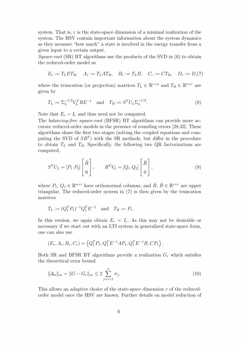
system. That is, r is the state-space dimension of a minimal realization of thesystem. The HSV contain important information about the system dynamicsas they measure “how much” a state is involved in the energy transfer from agiven input to a certain output.

Square-root (SR) BT algorithms use the products of the SVD in (6) to obtainthe reduced-order model as

Er := TLETR, Ar := TLATR, Br := TLB, Cr := CTR, Dr := D,(7)

where the truncation (or projection) matrices TL ∈ Rr×n and TR ∈ R

n×r aregiven by

TL := Σ−1/2L V T

L RE−1 and TR := ST ULΣ−1/2L . (8)

Note that Er = Ir and thus need not be computed.

The balancing-free square-root (BFSR) BT algorithms can provide more ac-curate reduced-order models in the presence of rounding errors [28,33]. Thesealgorithms share the first two stages (solving the coupled equations and com-puting the SVD of SRT ) with the SR methods, but differ in the procedureto obtain TL and TR. Specifically, the following two QR factorizations arecomputed,

ST UL = [P1 P2]

R

0

, RT VL = [Q1 Q2]

R

0

, (9)

where P1, Q1 ∈ Rn×r have orthonormal columns, and R, R ∈ R

r×r are uppertriangular. The reduced-order system in (7) is then given by the truncationmatrices

TL := (QT1 P1)

−1QT1 E−1 and TR := P1.

In this version, we again obtain Er = Ir. As this may not be desirable ornecessary if we start out with an LTI system in generalized state-space form,one can also use

(Er, Ar, Br, Cr) =(

QT1 P1, Q

T1 E−1AP1, Q

T1 E−1B,CP1

)

.

Both SR and BFSR BT algorithms provide a realization Gr which satisfiesthe theoretical error bound

‖∆a‖∞ = ‖G − Gr‖∞ ≤ 2n

∑

j=r+1

σj. (10)

This allows an adaptive choice of the state-space dimension r of the reduced-order model once the HSV are known. Further details on model reduction of

6

generalized LTI systems using BT methods, in particular when E is singular,are given in [29].

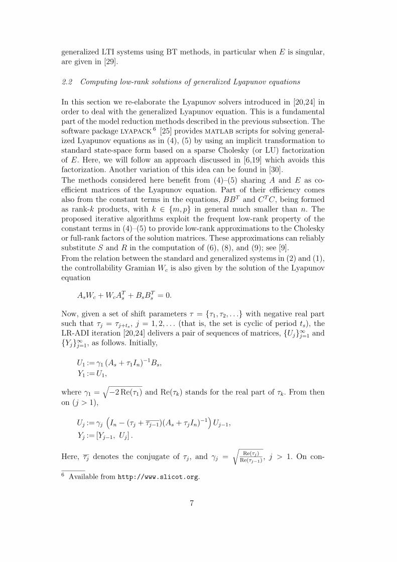
2.2 Computing low-rank solutions of generalized Lyapunov equations

In this section we re-elaborate the Lyapunov solvers introduced in [20,24] inorder to deal with the generalized Lyapunov equation. This is a fundamentalpart of the model reduction methods described in the previous subsection. Thesoftware package lyapack 6 [25] provides matlab scripts for solving general-ized Lyapunov equations as in (4), (5) by using an implicit transformation tostandard state-space form based on a sparse Cholesky (or LU) factorizationof E. Here, we will follow an approach discussed in [6,19] which avoids thisfactorization. Another variation of this idea can be found in [30].

The methods considered here benefit from (4)–(5) sharing A and E as co-efficient matrices of the Lyapunov equation. Part of their efficiency comesalso from the constant terms in the equations, BBT and CT C, being formedas rank-k products, with k ∈ {m, p} in general much smaller than n. Theproposed iterative algorithms exploit the frequent low-rank property of theconstant terms in (4)–(5) to provide low-rank approximations to the Choleskyor full-rank factors of the solution matrices. These approximations can reliablysubstitute S and R in the computation of (6), (8), and (9); see [9].

From the relation between the standard and generalized systems in (2) and (1),the controllability Gramian Wc is also given by the solution of the Lyapunovequation

AsWc + WcATs + BsB

Ts = 0.

Now, given a set of shift parameters τ = {τ1, τ2, . . .} with negative real partsuch that τj = τj+ts , j = 1, 2, . . . (that is, the set is cyclic of period ts), theLR-ADI iteration [20,24] delivers a pair of sequences of matrices, {Uj}∞j=1 and{Yj}∞j=1, as follows. Initially,

U1 := γ1 (As + τ1In)−1Bs,

Y1 := U1,

where γ1 =√

−2 Re(τ1) and Re(τk) stands for the real part of τk. From then

on (j > 1),

Uj := γj

(

In − (τj + τj−1)(As + τjIn)−1)

Uj−1,

Yj := [Yj−1, Uj] .

Here, τj denotes the conjugate of τj, and γj =√

Re(τj)

Re(τj−1), j > 1. On con-

6 Available from http://www.slicot.org.

7

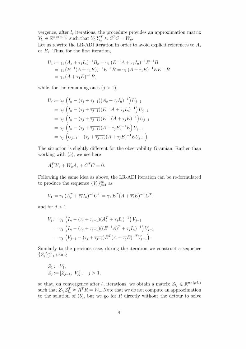
vergence, after lc iterations, the procedure provides an approximation matrixYlc ∈ R

n×(m·lc) such that YlcYTlc ≈ ST S = Wc.

Let us rewrite the LR-ADI iteration in order to avoid explicit references to As

or Bs. Thus, for the first iteration,

U1 := γ1 (As + τ1In)−1Bs = γ1 (E−1A + τ1In)−1E−1B

= γ1 (E−1(A + τ1E))−1E−1B = γ1 (A + τ1E)−1EE−1B

= γ1 (A + τ1E)−1B,

while, for the remaining ones (j > 1),

Uj := γj

(

In − (τj + τj−1)(As + τjIn)−1)

Uj−1

= γj

(

In − (τj + τj−1)(E−1A + τjIn)−1

)

Uj−1

= γj

(

In − (τj + τj−1)(E−1(A + τjE)−1

)

Uj−1

= γj

(

In − (τj + τj−1)(A + τjE)−1E)

Uj−1

= γj

(

Uj−1 − (τj + τj−1)(A + τjE)−1EUj−1

)

.

The situation is slightly different for the observability Gramian. Rather thanworking with (5), we use here

ATs Wo + WoAs + CT C = 0.

Following the same idea as above, the LR-ADI iteration can be re-formulatedto produce the sequence {Vj}∞j=1 as

V1 := γ1 (ATs + τ1In)−1CT = γ1 ET (A + τ1E)−T CT ,

and for j > 1

Vj := γj

(

In − (τj + τj−1)(ATs + τjIn)−1

)

Vj−1

= γj

(

In − (τj + τj−1)((E−1A)T + τjIn)−1

)

Vj−1

= γj

(

Vj−1 − (τj + τj−1)ET (A + τjE)−T Vj−1

)

.

Similarly to the previous case, during the iteration we construct a sequence{Zj}∞j=1 using

Z1 := V1,

Zj := [Zj−1, Vj] , j > 1,

so that, on convergence after lo iterations, we obtain a matrix Zlo ∈ Rn×(p·lo)

such that ZloZTlo ≈ RT R = Wo. Note that we do not compute an approximation

to the solution of (5), but we go for R directly without the detour to solve

8

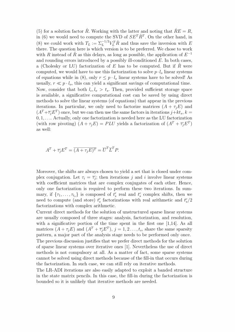
(5) for a solution factor R. Working with the latter and noting that RE = R,in (6) we would need to compute the SVD of SET RT . On the other hand, in

(8) we could work with TL := Σ−1/2L V T

L R and thus save the inversion with Ethere. The question here is which version is to be preferred. We chose to workwith R instead of R as this delays, as long as possible, the application of E−1

and rounding errors introduced by a possibly ill-conditioned E. In both cases,a (Cholesky or LU) factorization of E has to be computed. But if R werecomputed, we would have to use this factorization to solve p · lo linear systemsof equations while in (8), only r ≤ p · lo linear systems have to be solved! Asusually, r ≪ p · lo, this can yield a significant savings of computational time.

Now, consider that both lc, lo > ts. Then, provided sufficient storage spaceis available, a significative computational cost can be saved by using directmethods to solve the linear systems (of equations) that appear in the previousiterations. In particular, we only need to factorize matrices (A + τjE) and(AT +τjE

T ) once, but we can then use the same factors in iterations j+kts, k =0, 1, . . .. Actually, only one factorization is needed here as the LU factorization(with row pivoting) (A + τjE) = PLU yields a factorization of (AT + τjE

T )as well:

AT + τjET = (A + τjE)T = U

TL

TP.

Moreover, the shifts are always chosen to yield a set that is closed under com-plex conjugation. Let τi = τj; then iterations j and i involve linear systemswith coefficient matrices that are complex conjugates of each other. Hence,only one factorization is required to perform these two iterations. In sum-mary, if {τ1, . . . , τts} is composed of trs real and tcs complex shifts, then weneed to compute (and store) trs factorizations with real arithmetic and tcs/2factorizations with complex arithmetic.

Current direct methods for the solution of unstructured sparse linear systemsare usually composed of three stages: analysis, factorization, and resolution,with a significative portion of the time spent in the first one [1,14]. As allmatrices (A + τjE) and (AT + τjE

T ), j = 1, 2 . . . , ts, share the same sparsitypattern, a major part of the analysis stage needs to be performed only once.

The previous discussion justifies that we prefer direct methods for the solutionof sparse linear systems over iterative ones [1]. Nevertheless the use of directmethods is not compulsory at all. As a matter of fact, some sparse systemscannot be solved using direct methods because of the fill-in that occurs duringthe factorization. In such case, we can still rely on iterative methods.

The LR-ADI iterations are also easily adapted to exploit a banded structurein the state matrix pencils. In this case, the fill-in during the factorization isbounded so it is unlikely that iterative methods are needed.

9

2.2.1 Symmetric-definite state-matrix pencils

In case both A and E are symmetric, and one of them is definite, the corre-sponding matrix pencil only has real eigenvalues and is said to be symmetric-definite. In fact, because of the stability of A − λE, if A is negative definitethen E must be positive definite (and vice versa). In such case all shifts mustbe chosen to be real, and the iterations for Uj and Vj boil down to

U1 := γ1(A + τ1E)−1B,

Uj := γj

(

Uj−1 − (τj + τj−1)(A + τjE)−1EUj−1

)

, j > 1,

and

V1 := γ1E(A + τ1E)−1CT ,

Vj := γj

(

Vj−1 − (τj + τj−1)E(A + τjE)−1Vj−1

)

, j > 1,

where γj =√

τj

τj−1

.

As τj < 0 and A−λE is symmetric-definite stable, the matrix −(A+τjE)−1 issymmetric positive definite and the linear systems that appear in the iterationcan be solved via a (sparse) Cholesky factorization.

2.2.2 Selection of the shifts parameters

The performance of the previous iterations strongly depends on the selectionof the shift parameters.

For A or E unsymmetric, we propose to employ a modification of the heuristicproposed in [24] for standard LTI systems. This procedure delivers approxi-mations for the generalized eigenvalues of A − λE and (A − λE)−1 of largestmagnitude using the shift-and-invert Arnoldi iteration [15]. In such a case it isimportant that the set of selected shifts is closed under complex conjugation.

In case A − λE is symmetric definite, we utilize a procedure to computethe optimal shifts which requires estimators of both the largest and smallestmagnitude generalized eigenvalue of the pencil. Efficient codes to computethese approximations are based on generalizations of the Lanczos iteration.The shifts are then computed from these estimators with a negligible cost [8].

For further details on the convergence of the LR-ADI iteration and the prop-erties of the heuristic selection procedure, see [24,35].

2.2.3 Convergence criteria

The LR-ADI iterations present (at best) a superlinear convergence. A practicalstopping criterion is to halt the iteration when the contribution of the norm

of the columns that are added to the solution is relatively “small”. This isequivalent, e.g., to stop the computation of the sequences when

‖Uj‖F < ε · γ · ‖Yj‖F and ‖Vj‖F < ε · γ · ‖Zj‖F , (11)

10

where ε denotes the machine precision and γ is a tolerance threshold for theiteration; in our experiments we set γ := 100 · n.

A different approach requires computation of the relative residuals for theapproximations Yj and Zj to the solutions of the Lyapunov equations. Theidea here is to stop when the residuals

RWc(Yj) :=

‖A(YjYTj )ET + E(YjY

Tj )AT + BBT‖F

2‖A‖F‖E‖F‖YjY Tj ‖F + ‖BBT‖F

, (12)

RWo(Zj) :=

‖AT E−T (ZjZTj ) + (ZjZ

Tj )E−1A + CT C‖F

2‖A‖F‖E‖F‖E−T ZjZTj E−1‖F + ‖CT C‖F

, (13)

are smaller than a given tolerance threshold.

In practice, neither of these criteria (nor their combination) is completelysatisfactory and a “trial-and-error” approach together with careful monitoringof the iteration is necessary.

As the cost of computing the previous convergence criteria can be quite large(specially for the one based on the residuals), we propose to reduce it by usingthe following techniques:

1.) The norms of ‖Yj‖F and ‖Zj‖F can be computed incrementally. For ex-

ample, as Yj = [Yj−1, Uj], by construction ‖Yj‖F =√

‖Yj−1‖2F + ‖Uj‖2

F sothat only the norm of the n × m matrix Uj is required at each iterationstep.

2.) In several norm computations, we can avoid forming full dense n × nmatrices by using ‖MT M‖F = ‖MMT‖F . This is the case, e.g., whencomputing ‖YjY

Tj ‖F or ‖BBT‖F and implies a significant reduction both

in storage and computational costs.3.) We can also generalize the approach for computing the residual norms

in [26] as follows. Assume E is invertible; then YjYTj is an approximation

of the solution of

A(YjYTj )ET + E(YjY

Tj )AT + BBT = 0.

Let

M jc = [AYj, EYj, B] = Qj

cRjc = Qj

c [R1, R2, R3] (14)

be a (skinny) QR factorization of M jc , where Qj

c ∈ Rn×rq has rq = 2(j +

1)m orthonormal columns, and Rjc ∈ R

rq×rq is an upper triangular matrixpartitioned into blocks R1, R2, and R3 of j · m, j · m, and m columns,respectively. Then, we can use that

‖A(YjYTj )ET + E(YjY

Tj )AT + BBT‖F

11

= ‖ [AYj, EYj, B] [EYj, AYj, B]T ‖F = ‖M jc

0 Irq0

Irq0 0

0 0 Im

(M jc )T‖F

= ‖(M jc )T M j

c ‖F = ‖(Rjc)

T Rjc‖F = ‖RT

1 R1 + RT2 R2 + RT

3 R3‖F .

As the orthogonal factor need not be computed, the cost for this procedureis 2(nrq − 1

3r2q +(2j2 +1)m2)rq floating-point arithmetic operations (flops)

and thus increases in each step. Thus, if many iterations are required, thecost for evaluating the residual dominates the cost of the iteration even ifno full n × n matrices need be formed.

The idea is analogously derived for the residual (12).4.) Instead of evaluating the residual convergence criteria at each iteration,

we can do it periodically every few iterations.5.) The iterations for Yj and Zj can be dealt with independently so that one

of them can be stopped earlier.

2.2.4 Keeping the storage needs within limits

The LR-ADI iterations add m and p columns per step to the approximationfactors Yj and Zj. As these are dense matrices (with possibly complex entries),the storage needs of the algorithm increase by n(m + p) entries per iteration.In order to keep the required workspace within reasonable limits, we can com-press the matrices Yj and Zj during the iteration. Specifically, it is possible toreduce the number of columns in the factors by computing a rank-revealingQR (RRQR) factorizations [15]. For this purpose, we proceed to compute theRRQR factorization

Y Tj = QsRsΠs, rs := rank (Yj) = rank (Rs) ,

where Qs ∈ Rn×rs has orthonormal columns, Rs ∈ R

rs×rs is an upper triangu-lar matrix, and Πs is a square permutation matrix of order rs. Then, we cansubstitute Yj by its full-rank factor

Yj := RsΠTs .

A similar strategy delivers a compressed matrix for Zj. Whether the savingsin storage introduced by this column compression technique are worth thecost of the procedure depends on the rank of the computed factors. Also, theprocedure for evaluating the residuals (12) and (13) greatly benefits from areduction in the number of columns of Yj, Zj.

Traditionally the QR factorization with column pivoting [15] is employed forrank-revealing purposes because of its low computational cost and high relia-bility. (Although the SVD usually provides better accuracy, it does so at theexpense of a considerable higher cost. An SVD-based compression technique

12

is discussed in [17].) In [27] a BLAS-3 variant is proposed for this algorithmwhich maintains the same numerical behavior.

2.2.5 Computational savings using the LR-ADI solvers

It should be emphasized that the methods just described for solving (4)–(5)and computing (6) significantly differ from standard methods used in theMatlab toolboxes or SLICOT [34]. First, the proposed LR-ADI iteration forthe solution of the coupled Lyapunov equation has the potential to exploit thesparsity of the coefficient matrices A and E. Besides, as we are using low-rankapproximations to the full-rank or Cholesky factors, the computation of theSVD in (6) is usually less expensive: instead of a computational cost of O(n3)when using the Cholesky factors, this approach leads to an O(lcm · lop · n)cost where, in model reduction, often max{m, p} ≪ n; see [10]. If columncompression is applied, the cost of the SVD can be even more reduced. Howeverthen we need to pay for the cost of the column compression procedure.

The reduction of the cost of the SVD is an advantage shared by the routinesin our dense parallel model reduction library PLiCMR [10,3]. However, theroutines in PLiCMR cannot exploit the sparsity of the coefficient matrices ofthe Lyapunov equation.

2.3 Computational cost

For simplicity, we make the following assumptions in the evaluation of thecomputational cost of a serial implementation of the SR-BT model reductionalgorithm:

• Matrices A and E are unsymmetric. We refer to the number of nonzeros inthese matrices as z(A) and z(E), respectively.

• In case one of the state matrices M ∈ {A,E} presents a banded struc-ture, we denote by ku(M) and kl(M) the dimensions of its upper and lowerbandwidths, respectively.

• All the shifts {τ1, . . . , τts} are considered to be real.• Only computational costs, measured in flops, are considered. Minor order

terms are neglected in the expressions.

With the previous premises, the costs of a few basic sparse linear algebraoperations are introduced in Table 1.

The algorithm for model reduction is composed of four main stages: com-putation of shifts, LR-ADI iteration, SVD (of SRT ), and application of theSR formulae. Table 2 reports the operations involved in these stages togetherwith approximations of their computational costs. Only the cost for RWc

(Yj)is given, the cost for RWo

(Zj) being analogous.

13

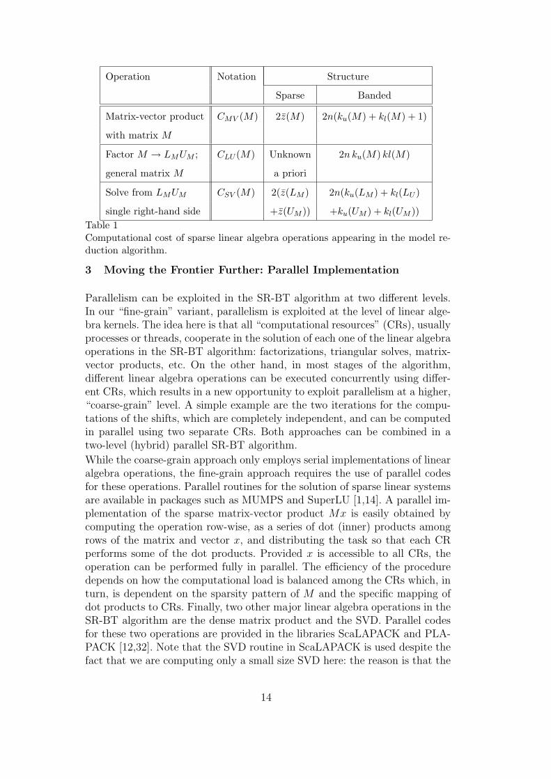
Operation Notation Structure

Sparse Banded

Matrix-vector product CMV (M) 2z(M) 2n(ku(M) + kl(M) + 1)

with matrix M

Factor M → LMUM ; CLU (M) Unknown 2n ku(M) kl(M)

general matrix M a priori

Solve from LMUM CSV (M) 2(z(LM ) 2n(ku(LM ) + kl(LU )

single right-hand side +z(UM )) +ku(UM ) + kl(UM ))

Table 1Computational cost of sparse linear algebra operations appearing in the model re-duction algorithm.

3 Moving the Frontier Further: Parallel Implementation

Parallelism can be exploited in the SR-BT algorithm at two different levels.In our “fine-grain” variant, parallelism is exploited at the level of linear alge-bra kernels. The idea here is that all “computational resources” (CRs), usuallyprocesses or threads, cooperate in the solution of each one of the linear algebraoperations in the SR-BT algorithm: factorizations, triangular solves, matrix-vector products, etc. On the other hand, in most stages of the algorithm,different linear algebra operations can be executed concurrently using differ-ent CRs, which results in a new opportunity to exploit parallelism at a higher,“coarse-grain” level. A simple example are the two iterations for the compu-tations of the shifts, which are completely independent, and can be computedin parallel using two separate CRs. Both approaches can be combined in atwo-level (hybrid) parallel SR-BT algorithm.

While the coarse-grain approach only employs serial implementations of linearalgebra operations, the fine-grain approach requires the use of parallel codesfor these operations. Parallel routines for the solution of sparse linear systemsare available in packages such as MUMPS and SuperLU [1,14]. A parallel im-plementation of the sparse matrix-vector product Mx is easily obtained bycomputing the operation row-wise, as a series of dot (inner) products amongrows of the matrix and vector x, and distributing the task so that each CRperforms some of the dot products. Provided x is accessible to all CRs, theoperation can be performed fully in parallel. The efficiency of the proceduredepends on how the computational load is balanced among the CRs which, inturn, is dependent on the sparsity pattern of M and the specific mapping ofdot products to CRs. Finally, two other major linear algebra operations in theSR-BT algorithm are the dense matrix product and the SVD. Parallel codesfor these two operations are provided in the libraries ScaLAPACK and PLA-PACK [12,32]. Note that the SVD routine in ScaLAPACK is used despite thefact that we are computing only a small size SVD here: the reason is that the

14

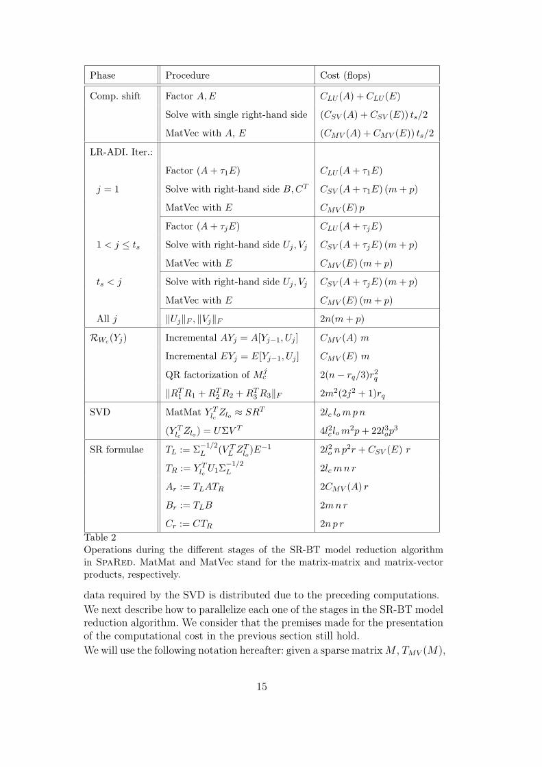
Phase Procedure Cost (flops)

Comp. shift Factor A, E CLU (A) + CLU (E)

Solve with single right-hand side (CSV (A) + CSV (E)) ts/2

MatVec with A, E (CMV (A) + CMV (E)) ts/2

LR-ADI. Iter.:

Factor (A + τ1E) CLU (A + τ1E)

j = 1 Solve with right-hand side B, CT CSV (A + τ1E) (m + p)

MatVec with E CMV (E) p

Factor (A + τjE) CLU (A + τjE)

1 < j ≤ ts Solve with right-hand side Uj , Vj CSV (A + τjE) (m + p)

MatVec with E CMV (E) (m + p)

ts < j Solve with right-hand side Uj , Vj CSV (A + τjE) (m + p)

MatVec with E CMV (E) (m + p)

All j ‖Uj‖F , ‖Vj‖F 2n(m + p)

RWc(Yj) Incremental AYj = A[Yj−1, Uj ] CMV (A) m

Incremental EYj = E[Yj−1, Uj ] CMV (E) m

QR factorization of M jc 2(n − rq/3)r2

q

‖RT1 R1 + RT

2 R2 + RT3 R3‖F 2m2(2j2 + 1)rq

SVD MatMat Y Tlc

Zlo ≈ SRT 2lc lo mp n

(Y Tlc

Zlo) = UΣV T 4l2c lo m2p + 22l3op3

SR formulae TL := Σ−1/2L (V T

L ZTlo

)E−1 2l2o n p2r + CSV (E) r

TR := Y Tlc

U1Σ−1/2L 2lc mn r

Ar := TLATR 2CMV (A) r

Br := TLB 2mn r

Cr := CTR 2n p r

Table 2Operations during the different stages of the SR-BT model reduction algorithmin SpaRed. MatMat and MatVec stand for the matrix-matrix and matrix-vectorproducts, respectively.

data required by the SVD is distributed due to the preceding computations.

We next describe how to parallelize each one of the stages in the SR-BT modelreduction algorithm. We consider that the premises made for the presentationof the computational cost in the previous section still hold.

We will use the following notation hereafter: given a sparse matrix M , TMV (M),

15

TLU(M), and TSV (M) stand, respectively, for the (sequential) times of comput-ing a matrix-vector product involving M , factorizing the matrix, and solvingthe corresponding triangular linear systems with a single RHS. These timesare directly proportional to the costs reflected in Table 1. (More specifically,TLU(M) and TSV (M) depend on the platform, the sparse solver that is em-ployed, and the structure of the coefficient matrix of the linear system.) Givendense matrices M1 and M2, TMM(M1M2) will be used for the (sequential)time to compute the dense matrix-matrix product M1M2, while TSD(M1) willdenote the (sequential) time for computing the SVD of M1. When the routineis executed in parallel, we will denote its time using a “p” superscript; thus,e.g., T P

MV (M) is the time to compute a (sparse) matrix-vector product withcoefficient matrix M using a certain parallel code. The superscripts “cp” and“fp” will denote coarse-grain and fine grain parallelism, respectively.

3.1 Computation of shifts

The two iterations in this stage require sparse matrix-vector products withAE−1 and EA−1, where the inversions are performed as two triangular solveseach given factorizations of A and E. The coefficient matrices only need tobe factorized once, and the triangular factors can be used as many times asneeded during the iteration. However, there is a strict dependence betweenconsecutive steps so that iteration j + 1 requires the results from iteration j.

The minimum execution time for the fine-grain parallelization of this stage is

T FPSHC = T P

LU(A) + T PLU(E)

+(T PSV (A) + T P

SV (E) + T PMV (A) + T P

MV (E)) ts/2,

which corresponds to having computed all operations in the stage, one by one,in parallel.

The coarse-grain approach to parallelizing the computation of shifts employstwo CRs to compute the two iterations independently. This results in thecoarse-grain parallel execution time

TCPSHC = max(TLU(A) + (TSV (A) + TMV (E)) ts/2,

TLU(E) + (TSV (E) + TMV (A)) ts/2).

Clearly, the maximum speed-up in this case is 2.

3.2 LR-ADI iteration

In order to better illustrate this stage, we will consider the following simplifi-cations:

• The first one performs the same operations as all the subsequent ones.• Both sequences perform the same number of iterations, lc = lo.

16

• The number of iterations is larger than the number of shifts, lc > ts.• The number of inputs equals the number of outputs of the system, m = p.• We will obviate the computation of the Frobenius norm for the sequences{Uj}∞j=1, {Vj}∞j=1, as well as the procedure to compute the residual normsassociated with the convergence criterion.

The fine-grain variant of this stage results in the parallel execution time

T FPADI = T P

LU(Fj) ts +(

T PSV (Fj) + T P

MV (E))

lc (m + p),

where Fj = A + τjE.

F2

F3

F4

F5

S1

S2

S3

S4

S5

S7

S6

S4

S3

S7

S6

S5

S1

S2

F1

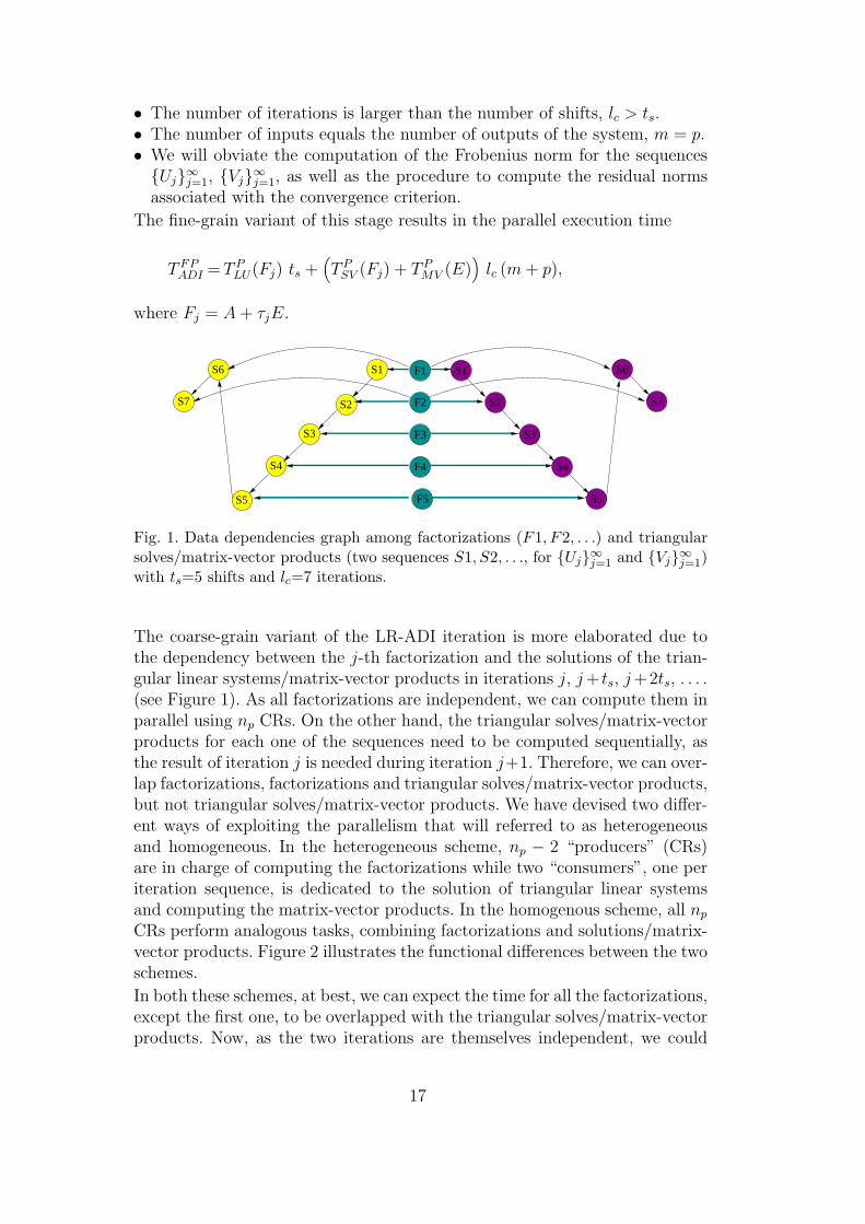
Fig. 1. Data dependencies graph among factorizations (F1, F2, . . .) and triangularsolves/matrix-vector products (two sequences S1, S2, . . ., for {Uj}∞j=1 and {Vj}∞j=1)with ts=5 shifts and lc=7 iterations.

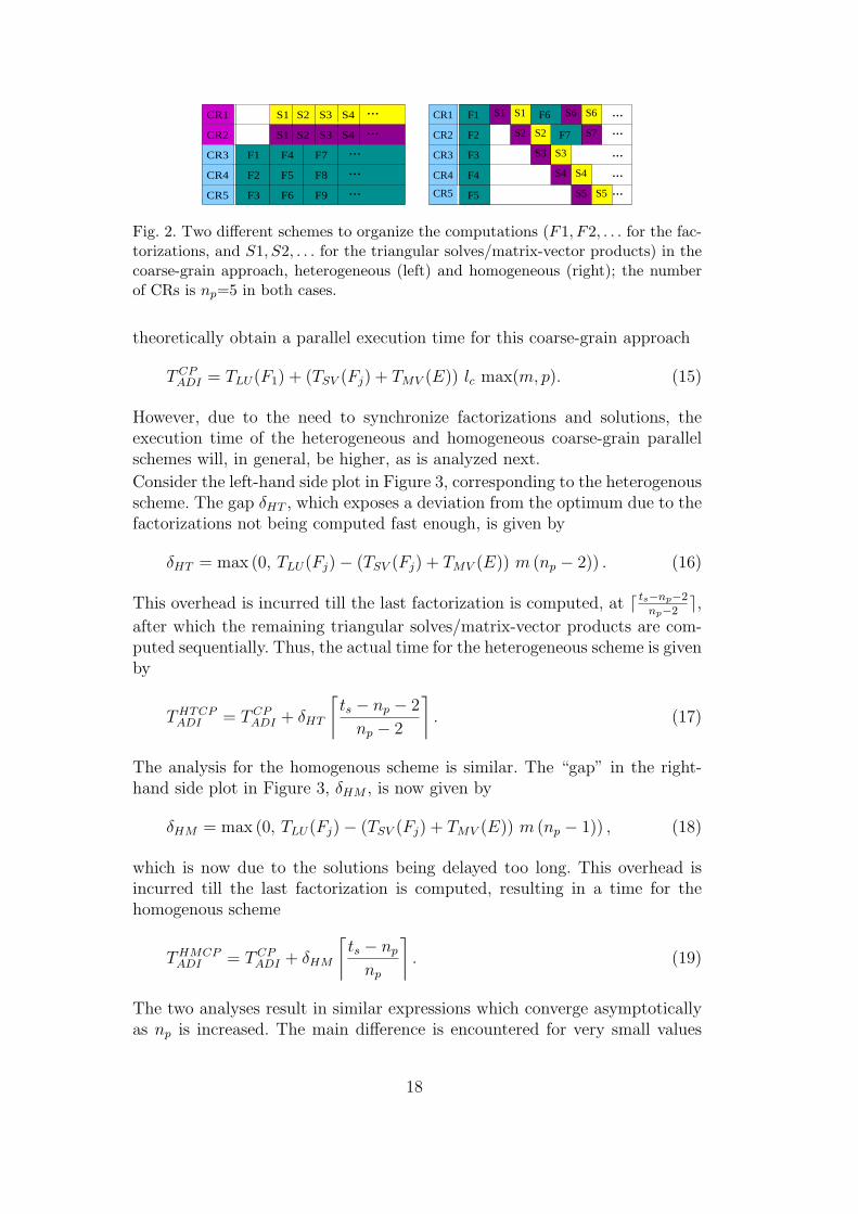
The coarse-grain variant of the LR-ADI iteration is more elaborated due tothe dependency between the j-th factorization and the solutions of the trian-gular linear systems/matrix-vector products in iterations j, j + ts, j +2ts, . . . .(see Figure 1). As all factorizations are independent, we can compute them inparallel using np CRs. On the other hand, the triangular solves/matrix-vectorproducts for each one of the sequences need to be computed sequentially, asthe result of iteration j is needed during iteration j+1. Therefore, we can over-lap factorizations, factorizations and triangular solves/matrix-vector products,but not triangular solves/matrix-vector products. We have devised two differ-ent ways of exploiting the parallelism that will referred to as heterogeneousand homogeneous. In the heterogeneous scheme, np − 2 “producers” (CRs)are in charge of computing the factorizations while two “consumers”, one periteration sequence, is dedicated to the solution of triangular linear systemsand computing the matrix-vector products. In the homogenous scheme, all np

CRs perform analogous tasks, combining factorizations and solutions/matrix-vector products. Figure 2 illustrates the functional differences between the twoschemes.

In both these schemes, at best, we can expect the time for all the factorizations,except the first one, to be overlapped with the triangular solves/matrix-vectorproducts. Now, as the two iterations are themselves independent, we could

17

...S1 S2 S3 S4

F1

F2

F3

F4

F5

F6

F7

F8

F9

...

...

...

CR3

CR2

CR4

CR5

CR1 ...S1 S2 S3 S4 F1

F2

F3

F4

S2

S1

S3

S4

S6

S7F7

S3

S4

S6S1 F6

S2

F5 S5 S5

CR1

CR2

CR3

CR4

CR5

...

...

...

...

...

Fig. 2. Two different schemes to organize the computations (F1, F2, . . . for the fac-torizations, and S1, S2, . . . for the triangular solves/matrix-vector products) in thecoarse-grain approach, heterogeneous (left) and homogeneous (right); the numberof CRs is np=5 in both cases.

theoretically obtain a parallel execution time for this coarse-grain approach

TCPADI = TLU(F1) + (TSV (Fj) + TMV (E)) lc max(m, p). (15)

However, due to the need to synchronize factorizations and solutions, theexecution time of the heterogeneous and homogeneous coarse-grain parallelschemes will, in general, be higher, as is analyzed next.

Consider the left-hand side plot in Figure 3, corresponding to the heterogenousscheme. The gap δHT , which exposes a deviation from the optimum due to thefactorizations not being computed fast enough, is given by

δHT = max (0, TLU(Fj) − (TSV (Fj) + TMV (E)) m (np − 2)) . (16)

This overhead is incurred till the last factorization is computed, at ⌈ ts−np−2np−2

⌉,after which the remaining triangular solves/matrix-vector products are com-puted sequentially. Thus, the actual time for the heterogeneous scheme is givenby

THTCPADI = TCP

ADI + δHT

⌈

ts − np − 2

np − 2

⌉

. (17)

The analysis for the homogenous scheme is similar. The “gap” in the right-hand side plot in Figure 3, δHM , is now given by

δHM = max (0, TLU(Fj) − (TSV (Fj) + TMV (E)) m (np − 1)) , (18)

which is now due to the solutions being delayed too long. This overhead isincurred till the last factorization is computed, resulting in a time for thehomogenous scheme

THMCPADI = TCP

ADI + δHM

⌈

ts − np

np

⌉

. (19)

The two analyses result in similar expressions which converge asymptoticallyas np is increased. The main difference is encountered for very small values

18

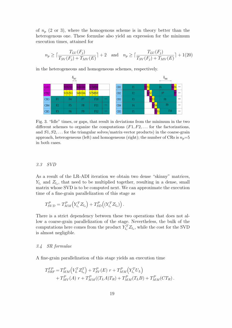
of np (2 or 3), where the homogenous scheme is in theory better than theheterogenous one. These formulae also yield an expression for the minimumexecution times, attained for

np ≥ ⌈ TLU(Fj)

TSV (Fj) + TMV (E)⌉ + 2 and np ≥ ⌈ TLU(Fj)

TSV (Fj) + TMV (E)⌉ + 1(20)

in the heterogeneous and homogeneous schemes, respectively.

F4 F7

F8

F6

δHT

F11

F12

...

...

...F5

F1 F10

S1

S2S3

S3

S7

S7

S8

S8S9

S4

S4

S5S6

S2 S5S6

S9

F2

F3 F9

CR3

CR2

CR4

CR5

CR1 S1

CR4

CR3

CR1

CR2

CR5

F1 S6

S2S2

S6F6S1S1 S6

S7

S6 ..................

F7

F3

F5

F2

F4

S3

S4

S5

S3

S4

S5

δHM

F9

F8

F10

Fig. 3. “Idle” times, or gaps, that result in deviations from the minimum in the twodifferent schemes to organize the computations (F1, F2, . . . for the factorizations,and S1, S2, . . . for the triangular solves/matrix-vector products) in the coarse-grainapproach, heterogeneous (left) and homogeneous (right); the number of CRs is np=5in both cases.

3.3 SVD

As a result of the LR-ADI iteration we obtain two dense “skinny” matrices,Ylc and Zlo , that need to be multiplied together, resulting in a dense, smallmatrix whose SVD is to be computed next. We can approximate the executiontime of a fine-grain parallelization of this stage as

T PSV D = T P

MM

(

Y Tlc Zlo

)

+ T PSD

(

(Y Tlc Zlo)

)

.

There is a strict dependency between these two operations that does not al-low a coarse-grain parallelization of the stage. Nevertheless, the bulk of thecomputations here comes from the product Y T

lc Zlo , while the cost for the SVDis almost negligible.

3.4 SR formulae

A fine-grain parallelization of this stage yields an execution time

T FPSRF = T P

MM

(

V TL ZT

lo

)

+ T PSV (E) r + T P

MM

(

Y Tlc UL

)

+ T PMV (A) r + T P

MM((TLA)TR) + T PMM(TLB) + T P

MM(CTR) .

19

Alternatively, we could calculate TL and TR in two different CRs and, oncethese projectors are available, obtain the matrices of the reduced-order systemusing three CRs. This yields the parallel execution time

TCPSRF = max

(

TMM

(

V TL ZT

lo

)

+ TSV (E) r, TMM

(

Y Tlc UL

))

+ max(TMV (A) r + TMM((TLA)TR) , TMM(TLB) , TMM(CTR)).

3.5 Overlapping stages

There is still some more parallelism that can be extracted from part of theSR-BT model reduction algorithm. Consider the product Y T

lc Zlo needed tocompute the SVD. Assume we are just about to start step j in the LR-ADI it-eration so that Yj−1/Zj−1, composed of (j−1)m/(j−1)p columns, are known,and consider we have already computed the product Y T

j−1Zj−1. Then, duringiteration j, Uj/Vj are computed so that Yj = [Yj−1, Uj] and Zj = [Zj−1, Vj].Therefore, using one additional CR, we can overlap the computations cor-responding to step j + 1 of the LR-ADI iteration with the products Y T

j−1Uj,V T

j Zj−1, and UTj Vj that are necessary as part of the construction of the overall

product Y Tlc Zlo . Proceeding in this manner, a major bulk of the computation of

the product can be overlapped with the LR-ADI iteration. Note that formingthis product is the major part of the SVD stage, so that overlapping can hereyield a significant reduction in the total computational time.

A second overlap can be attained by rearranging the computation of the pro-jector TL := Σ

−1/2L (V T

L ZTlo)E

−1 so that the linear system ZTloE

−1 is solved first,and then the matrix product of V T

L with this partial result is computed. Al-though this increases the overall cost of the procedure, the solution of thelinear system can be then overlapped with the LR-ADI iteration resulting ina lower execution time.

3.6 Threads vs. processes as CRs

The fine-grain variants require parallel implementations of several linear alge-bra operations. Thread-level parallelism can be exploited by simply linking inmultithreaded implementations of BLAS (e.g., Intel MKL 7 or GotoBLAS 8 ),both for sparse and dense linear algebra operations. To exploit process-levelparallelism, we can use message-passing packages as, e.g., MUMPS or Su-perLU for sparse linear algebra, or ScaLAPACK, the message-passing versionof LAPACK, for dense linear algebra.

The coarse-grain variants can be implemented using higher level tools for theshared-memory and the message-passing programming models as OpenMPand MPI. Naturally, thread-level parallelism is only appropriate for shared-

7 Available from http://www.intel.org.8 Available from http://www.tacc.utexas.edu/resources/software.

20

memory multiprocessors (SMM). The process-level/message passing combina-tion is possible both in SMM and distributed-memory platforms (multicom-puters).

Consider now the coarse-grain heterogeneous and homogeneous schemes forthe LR-ADI iteration. The former computes the solutions in two CRs (theconsumers) so that factorizations computed at any other CRs need to bestreamlined through these. This can result in a high volume of data movement(This is clearly true in multicomputers, but also in shared-memory platformswith a ccNUMA or NUMA organization). In the homogeneous scheme, it isthe solutions that are to be passed between “neighbour” CRs. Therefore, wecan expect the amount of data movement to be lower in this scheme.

The hybrid two-level approach could be easily implemented by combiningprocesses at the coarse-level and threads at the fine-grain level. However, thisimplementation is not considered further as thread-safe implementations ofthe linear algebra libraries are needed and, unfortunately, as to date, MUMPSdoes not satisfy this property.

4 Numerical Experiments

All the experiments presented in this section were performed on a ccNUMASGI Altix 350 platform with 8 nodes using ieee double-precision floating-pointarithmetic (ε ≈ 2.2204e−16). Each node consists of two Intel Itanium 2 pro-cessors@1.5 GHz with 2 GBytes of RAM. We employ a BLAS library speciallytuned for this processor that achieves around 5300 Mflops (millions of flopsper second) for the matrix product (routine DGEMM in MKL 8.0). The nodesare connected via an SGI NUMAlink network and the MPI communicationlibrary is specially developed and tuned for this network.

All results were obtained using the SR-BT algorithm in our library SpaRed.We found no significative difference when using the BFSR-BT code for theexamples reported in the following.

4.1 Model reduction benchmarks

In the evaluation we employ several examples coming from two different bench-marks: the first one is part of the NICONET project 9 , which led to the devel-opment of the SLICOT library 10 , and includes several small-scale examples forstandard realizations (E = In) with unsymmetric sparse state matrix A [13].The second benchmark is the result of a recent effort to assemble large-scaleexamples in the Oberwolfach model reduction collection coordinated at theUniversity of Freiburg 11 . Table 3 and the following brief description feature

9 http://www.icm.tu-bs.de/NICONET10 http://www.slicot.org11 http://www.imtek.de/simulation/benchmark/

21

some of the relevant aspects of the models.

CD player (C DISC). This example is frequently used as a benchmark formodel reduction. The system describes the dynamic behavior of the mech-anisms of the swing arm and the lens of a portable Compact Disc player.The goal is to obtain a low-cost controller which is both fast and robust toexternal shocks.

Random model (RAND). This is a randomly generated single-input, single-output model. There is no real application behind this example.

Hospital building (BUILD I). This example comes from modeling vibra-tions of a building at Los Angeles University Hospital. The model is dis-cretized with 8 floors and 3 degrees of freedom each, which correspond tothe displacements in the x and y directions, and the rotation. A second-order differential equation is thus obtained which is then transformed intoan standard continuous-time LTI system.

Clamped beam (BEAM). This system results from the discretization ofa hyperbolic PDE modeling a clamped beam with proportional damping,resulting in a second-order system. Here the input contains the force appliedto the structure while the output represents the corresponding displacement.

Russian service module ISS (ISS I). This is a (linearized second-order)system modeling component 1R of the International Space Station (ISS).The challenge is to control a flexible structure in space in real-time so thatit becomes necessary to reduce the flex models in order to complete theanalysis in a timely manner.

Extended service module ISS (ISS II). This model corresponds to a sec-ond assembly stage of the ISS, also known as module 12A. The goal of modelreduction here is similar to that of the previous example.

Optimal cooling of steel profiles (STEEL I and STEEL II). This modelarises in a manufacturing method for steel profiles [11,31]. The goal is to de-sign a control that achieves moderate temperature gradients when the rail iscooled down. The mathematical model corresponds to the boundary controlfor a 2-D heat equation. A finite element discretization, followed by adaptiverefinement of the mesh result in the two examples in this benchmark.

Micropyros thruster (T3DL). This is a model of a microthruster arraybased on the co-integration of solid fuel with a silicon micromachined sys-tem [21]. The design problem is to reach the critical temperature withinthe fuel but, at the same time, do not reach the critical temperature at theneighboring microthrusters. The model for the device was constructed andmeshed using ANSYS.

Chip cooling model (CHIP). This is a design corresponding to a 3-D modelof a chip cooled by forced convection that is used in the thermal simulationof heat exchange between a solid body (the chip) and a fluid flow.

22

SLICOT benchmark collection

Example n m p z(A) z(E)

C DISC 120 2 2 240 = z(In)

RAND 200 1 1 2,132 = z(In)

BUILD I 48 1 1 1,176 = z(In)

BEAM 348 1 1 60,726 = z(In)

ISS I 270 3 3 405 = z(In)

ISS II 1,412 3 3 2,118 = z(In)

Oberwolfach benchmark collection

Example n m p z(A) z(E)

STEEL I 20,209 7 6 139,233 139,473

STEEL II 79,841 7 6 553,921 554,913

T3DL 20,360 1 7 265,113 20,360

CHIP 20,082 1 5 281,150 20,082

Table 3Examples included in the evaluation of the SpaRed model reduction routine.

4.2 Numerical performance of the Lyapunov solver

We first study the convergence rate and the numerical performance of the LR-ADI Lyapunov solvers. Table 4 reports, for each example, the number of shiftsused for the iteration, ts, the number of iterations required for convergence,lc, the relative contribution of the last columns added to the solution (11),and the residuals (12)–(13) after lc iterations. As the convergence is stronglydependent on the selection and the number of shifts, repeated executions wereperformed in order to choose those values reported in the table.

A few comments are worth about the results in the table:

• The iteration did not converge according to any of the criteria for examplesC DISC, BUILD I, ISS I, ISS II, and T3DL. (Due to the scale of problemT3DL, we only allowed 140 iterations for this case.) Although the residualsRWc

(Ylc) and RWo(Zlo) can be considered small for the former two examples,

both ISS examples offers poor residuals. Example T3DL also offer unsatis-factory residuals for one of the equations. Notice however that the qualityof the solutions should be judged by the soundness of the reduced-ordersystems, to be evaluated in short.

• The convergence criterion based on the contribution of the columns addedto the solution is appropriate for examples BEAM, STEEL I, STEEL II,and CHIP.

23

Example ts lc‖Ulc‖F

‖Ylc‖F

‖Vlc‖F

‖Zlo‖FRWc

(Ylc) RWo(Zlo))

C DISC 25 1,000 1.24e−05 1.24e−05 1.36e−11 1.33e−11

RAND 20 40 6.29e−08 6.94e−08 1.47e−16 1.20e−16

BUILD I 40 1,000 9.87e−06 4.40e−05 7.30e−12 4.29e−11

BEAM 20 40 1.96e−03 5.90e−04 2.06e−08 2.17e−09

ISS I 20 1,000 1.24e−03 1.41e−03 6.02e−07 2.11e−05

ISS II 20 1,000 1.17e−02 1.74e−03 9.36e−06 3.35e−06

STEEL I 25 76 4.25e−10 4.21e−11 2.94e−09 4.89e−20

STEEL II 26 78 1.63e−10 1.59e−09 1.80e−08 4.54e−21

T3DL 29 140 1.45e−02 1.49e−02 4.04e+00 1.32e−12

CHIP 20 59 1.43e−10 5.00e−11 4.45e−09 1.28e−25

Table 4Convergence and numerical performance of LR-ADI iteration routine.

• The LR-ADI iteration for the RAND example was stopped after only 40iterations with residuals as low as one could expect. The convergence cri-terion based on the residuals, combined with a careful monitoring, servedits purpose for this example as we detected that no improvement in theresiduals was obtained by iterating further.

4.3 Numerical performance of the SR-BT model reduction algorithm

We next compare the frequency response of the original systems with thatof the reduced-order realizations obtained using SpaRed. For the small-scaleproblems in SLICOT, we include a reliable BT model reduction routine fromPLiCMR in the experiments. The kernels in PLiCMR, though parallel, do notpreserve nor exploit the sparsity of E or A, and therefore cannot deal withthe large examples from the Oberwolfach benchmark.

Both the SpaRed and the PLiCMR routines select the order r automaticallyso that

σr > max(γ1, n · ε · σ1) > σr+1,

where ε is the machine precision and γ1 is a user-specified tolerance threshold.In our case, we set γ1 = η · σ1, with the value η adjusted for each particularexample. Obviously, a larger order provides a more accurate model, but alsoincreases the cost of latter computations involving the reduced-order model.For each example, Table 5 shows the values of r and σ1, and the theoreticalerror bound ∆a the reduced-order realization must satisfy (see (10)). As ameasure of the quality of the reduced-order systems, in the table we also

24

report the difference

‖G − Gr‖∞ = σmax(G − Gr);

here, the TFMs are evaluated at w, with w composed of 1,000 frequencysamples logarithmically distributed in the interval [fmin, fmax], and fmin andfmax chosen specifically for each different example.

Example r σ1 ∆a [fmin, fmax] SpaRed PLiCMR

‖G − Gr‖∞ ‖G − Gr‖∞

C DISC 42 1.17e+6 2.35e−01 [1e−1,1e+5] 1.64e−2 1.64e−2

RAND 7 8.19e+6 1.79e+01 [1e+1,1e+5] 6.29e+0 6.29e+0

BUILD I 30 2.50e−3 2.69e−05 [1e−1,1e+3] 4.92e−6 4.92e−6

BEAM 12 2.38e+3 1.24e+01 [1e−2,1e+3] 2.98e+0 2.37e+0

ISS I 36 5.79e−3 1.83e−03 [1e−2,1e+3] 2.03e−3 8.61e−5

ISS II 66 5.84e−3 4.21e−02 [1e−2,1e+3] 7.06e−3 7.38e−4

STEEL I 45 2.55e−2 1.47e−04 [1e−2,1e+6] 1.54e−5 –

STEEL II 60 2.57e−2 4.56e−06 [1e−2,1e+6] 5.29e−6 –

T3DL 30 2.81e+2 2.16e−06 [1e+0,1e+8] 6.74e−4 –

CHIP 40 5.27e+1 6.71e−10 [1e+0,1e+5] 3.35e−10 –

Table 5Numerical performance of SpaRed model reduction routine.

A close inspection of the results in the table reveals the following:

• All the examples satisfy the theoretical bound, except for the ISS I andT3DL examples computed using the SpaRed routine. We can impute thison the low quality of the approximations to the solutions of the Gramiansproduced by the LR-ADI iteration for these particular examples.

• A comparison between the SpaRed and PLiCMR codes reports close resultsexcept for the two ISS examples, where PLiCMR performs better.

• It is quite remarkable that models of order 45 and 60 are enough to capturethe dynamics of the large systems of the STEEL examples.

The measure ‖G−Gr‖∞ compresses all the information relative to the absoluteerror of the reduced-order system into a single number. However, in general itis more enlightening to analyze the frequency response dynamics and its errorover the relevant frequency spectrum. Figures 4–7 report next the frequencyresponses

|Gik( ω)|, 1 ≤ k ≤ p, 1 ≤ i ≤ m,

of the transfer function from input i to output k for the examples in the SLI-

25

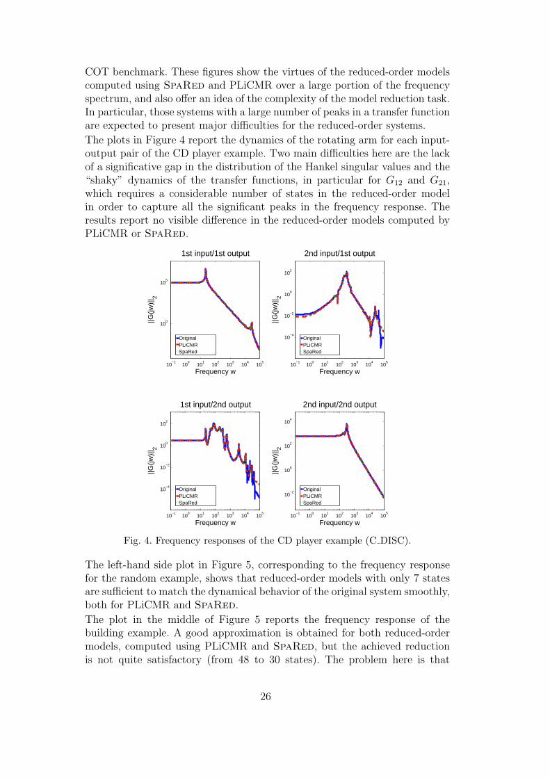
COT benchmark. These figures show the virtues of the reduced-order modelscomputed using SpaRed and PLiCMR over a large portion of the frequencyspectrum, and also offer an idea of the complexity of the model reduction task.In particular, those systems with a large number of peaks in a transfer functionare expected to present major difficulties for the reduced-order systems.

The plots in Figure 4 report the dynamics of the rotating arm for each input-output pair of the CD player example. Two main difficulties here are the lackof a significative gap in the distribution of the Hankel singular values and the“shaky” dynamics of the transfer functions, in particular for G12 and G21,which requires a considerable number of states in the reduced-order modelin order to capture all the significant peaks in the frequency response. Theresults report no visible difference in the reduced-order models computed byPLiCMR or SpaRed.

10−1

100

101

102

103

104

105

100

105

Frequency w

||G(jw

)|| 2

1st input/1st output

OriginalPLiCMRSpaRed

10−1

100

101

102

103

104

105

10−4

10−2

100

102

Frequency w

||G(jw

)|| 2

2nd input/1st output

OriginalPLiCMRSpaRed

10−1

100

101

102

103

104

105

10−4

10−2

100

102

Frequency w

||G(jw

)|| 2

1st input/2nd output

OriginalPLiCMRSpaRed

10−1

100

101

102

103

104

105

10−2

100

102

104

Frequency w

||G(jw

)|| 2

2nd input/2nd output

OriginalPLiCMRSpaRed

Fig. 4. Frequency responses of the CD player example (C DISC).

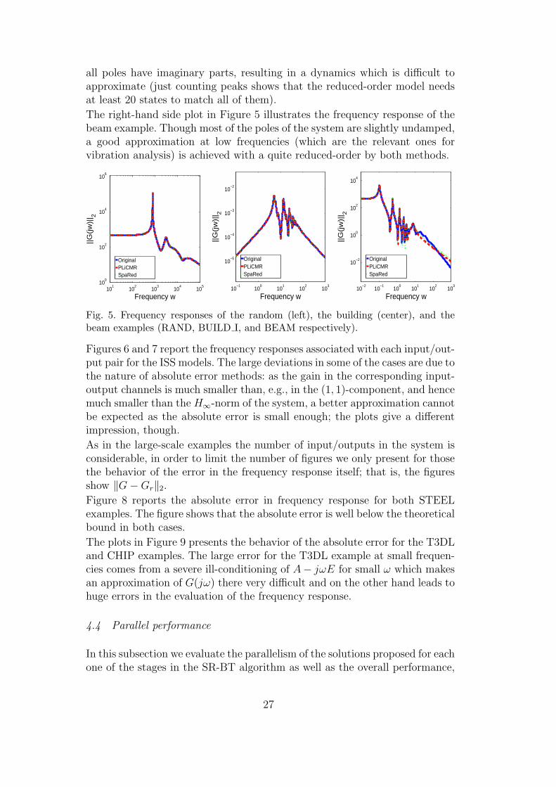
The left-hand side plot in Figure 5, corresponding to the frequency responsefor the random example, shows that reduced-order models with only 7 statesare sufficient to match the dynamical behavior of the original system smoothly,both for PLiCMR and SpaRed.

The plot in the middle of Figure 5 reports the frequency response of thebuilding example. A good approximation is obtained for both reduced-ordermodels, computed using PLiCMR and SpaRed, but the achieved reductionis not quite satisfactory (from 48 to 30 states). The problem here is that

26

all poles have imaginary parts, resulting in a dynamics which is difficult toapproximate (just counting peaks shows that the reduced-order model needsat least 20 states to match all of them).

The right-hand side plot in Figure 5 illustrates the frequency response of thebeam example. Though most of the poles of the system are slightly undamped,a good approximation at low frequencies (which are the relevant ones forvibration analysis) is achieved with a quite reduced-order by both methods.

101

102

103

104

105

100

102

104

106

Frequency w

||G(jw

)|| 2

OriginalPLiCMRSpaRed

10−1

100

101

102

103

10−5

10−4

10−3

10−2

Frequency w

||G

(jw

)|| 2

OriginalPLiCMRSpaRed

10−2

10−1

100

101

102

103

10−2

100

102

104

Frequency w

||G

(jw

)|| 2

OriginalPLiCMRSpaRed

Fig. 5. Frequency responses of the random (left), the building (center), and thebeam examples (RAND, BUILD I, and BEAM respectively).

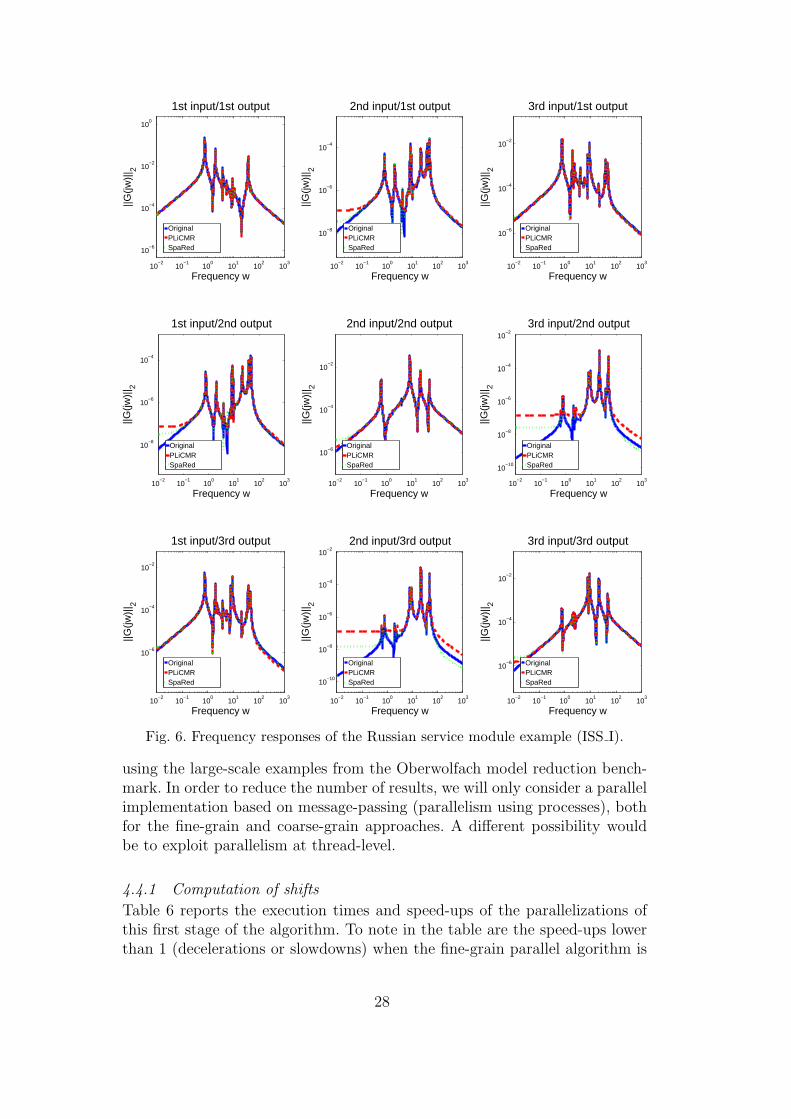
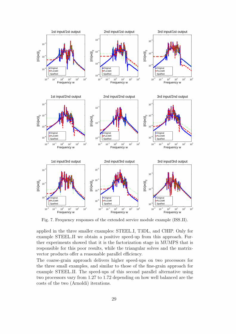
Figures 6 and 7 report the frequency responses associated with each input/out-put pair for the ISS models. The large deviations in some of the cases are due tothe nature of absolute error methods: as the gain in the corresponding input-output channels is much smaller than, e.g., in the (1, 1)-component, and hencemuch smaller than the H∞-norm of the system, a better approximation cannotbe expected as the absolute error is small enough; the plots give a differentimpression, though.

As in the large-scale examples the number of input/outputs in the system isconsiderable, in order to limit the number of figures we only present for thosethe behavior of the error in the frequency response itself; that is, the figuresshow ‖G − Gr‖2.

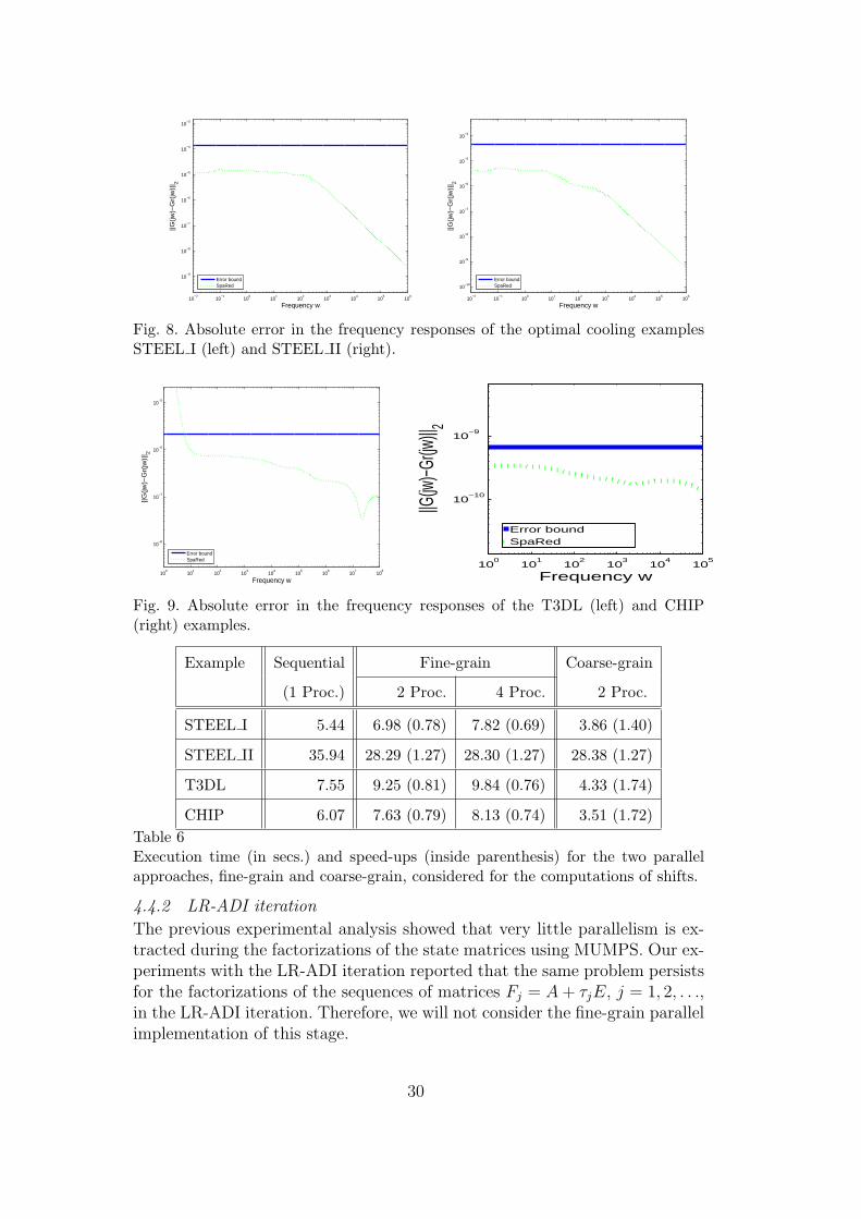
Figure 8 reports the absolute error in frequency response for both STEELexamples. The figure shows that the absolute error is well below the theoreticalbound in both cases.

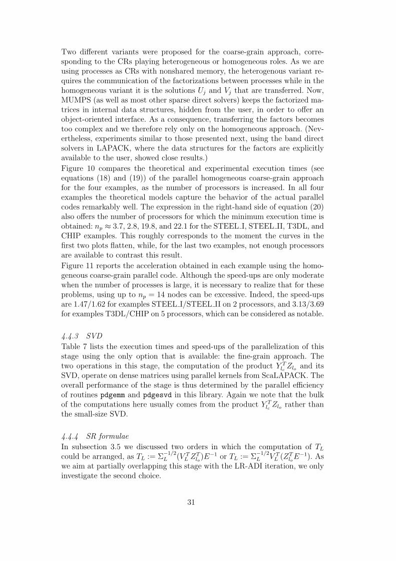
The plots in Figure 9 presents the behavior of the absolute error for the T3DLand CHIP examples. The large error for the T3DL example at small frequen-cies comes from a severe ill-conditioning of A− jωE for small ω which makesan approximation of G(jω) there very difficult and on the other hand leads tohuge errors in the evaluation of the frequency response.

4.4 Parallel performance

In this subsection we evaluate the parallelism of the solutions proposed for eachone of the stages in the SR-BT algorithm as well as the overall performance,

27

10−2

10−1

100

101

102

103

10−6

10−4

10−2

100

Frequency w

||G(jw

)|| 2

1st input/1st output

OriginalPLiCMRSpaRed

10−2

10−1

100

101

102

103

10−8

10−6

10−4

Frequency w

||G(jw

)|| 2

2nd input/1st output

OriginalPLiCMRSpaRed

10−2

10−1

100

101

102

103

10−6

10−4

10−2

Frequency w

||G(jw

)|| 2

3rd input/1st output

OriginalPLiCMRSpaRed

10−2

10−1

100

101

102

103

10−8

10−6

10−4

Frequency w

||G(jw

)|| 2

1st input/2nd output

OriginalPLiCMRSpaRed

10−2

10−1

100

101

102

103

10−6

10−4

10−2

Frequency w

||G(jw

)|| 2

2nd input/2nd output

OriginalPLiCMRSpaRed

10−2

10−1

100

101

102

103

10−10

10−8

10−6

10−4

10−2

Frequency w||G

(jw)|

| 2

3rd input/2nd output

OriginalPLiCMRSpaRed

10−2

10−1

100

101

102

103

10−6

10−4

10−2

Frequency w

||G(jw

)|| 2

1st input/3rd output

OriginalPLiCMRSpaRed

10−2

10−1

100

101

102

103

10−10

10−8

10−6

10−4

10−2

Frequency w

||G(jw

)|| 2

2nd input/3rd output

OriginalPLiCMRSpaRed

10−2

10−1

100

101

102

103

10−6

10−4

10−2

Frequency w

||G(jw

)|| 2

3rd input/3rd output

OriginalPLiCMRSpaRed

Fig. 6. Frequency responses of the Russian service module example (ISS I).

using the large-scale examples from the Oberwolfach model reduction bench-mark. In order to reduce the number of results, we will only consider a parallelimplementation based on message-passing (parallelism using processes), bothfor the fine-grain and coarse-grain approaches. A different possibility wouldbe to exploit parallelism at thread-level.

4.4.1 Computation of shifts

Table 6 reports the execution times and speed-ups of the parallelizations ofthis first stage of the algorithm. To note in the table are the speed-ups lowerthan 1 (decelerations or slowdowns) when the fine-grain parallel algorithm is

28

10−2

10−1

100

101

102

103

10−6

10−4

10−2

Frequency w

||G(jw

)|| 2

1st input/1st output

OriginalPLiCMRSpaRed

10−2

10−1

100

101

102

103

10−8

10−6

10−4

10−2

Frequency w

||G(jw

)|| 2

2nd input/1st output

OriginalPLiCMRSpaRed

10−2

10−1

100

101

102

103

10−6

10−4

10−2

Frequency w

||G(jw

)|| 2

3rd input/1st output

OriginalPLiCMRSpaRed

10−2

10−1

100

101

102

103

10−8

10−6

10−4

10−2

Frequency w

||G(jw

)|| 2

1st input/2nd output

OriginalPLiCMRSpaRed

10−2

10−1

100

101

102

103

10−6

10−4

10−2

Frequency w

||G(jw

)|| 2

2nd input/2nd output

OriginalPLiCMRSpaRed

10−2

10−1

100

101

102

103

10−8

10−6

10−4

10−2

Frequency w||G

(jw)|

| 2

3rd input/2nd output

OriginalPLiCMRSpaRed

10−2

10−1

100

101

102

103

10−6

10−4

10−2

Frequency w

||G(jw

)|| 2

1st input/3rd output

OriginalPLiCMRSpaRed

10−2

10−1

100

101

102

103

10−8

10−6

10−4

10−2

Frequency w

||G(jw

)|| 2

2nd input/3rd output

OriginalPLiCMRSpaRed

10−2

10−1

100

101

102

103

10−6

10−4

10−2

Frequency w

||G(jw

)|| 2

3rd input/3rd output

OriginalPLiCMRSpaRed

Fig. 7. Frequency responses of the extended service module example (ISS II).

applied in the three smaller examples: STEEL I, T3DL, and CHIP. Only forexample STEEL II we obtain a positive speed-up from this approach. Fur-ther experiments showed that it is the factorization stage in MUMPS that isresponsible for this poor results, while the triangular solves and the matrix-vector products offer a reasonable parallel efficiency.

The coarse-grain approach delivers higher speed-ups on two processors forthe three small examples, and similar to those of the fine-grain approach forexample STEEL II. The speed-ups of this second parallel alternative usingtwo processors vary from 1.27 to 1.72 depending on how well balanced are thecosts of the two (Arnoldi) iterations.

29

10−2

10−1

100

101

102

103

104

105

106

10−9

10−8

10−7

10−6

10−5

10−4

10−3

Frequency w

||G(jw

)−G

r(jw

)|| 2

Error boundSpaRed

10−2

10−1

100

101

102

103

104

105

106

10−10

10−9

10−8

10−7

10−6

10−5

10−4

Frequency w

||G(jw

)−G

r(jw

)|| 2

Error boundSpaRed

Fig. 8. Absolute error in the frequency responses of the optimal cooling examplesSTEEL I (left) and STEEL II (right).

100

101

102

103

104

105

106

107

108

10−8

10−7

10−6

10−5

Frequency w

||G(jw

)−G

r(jw

)|| 2

Error boundSpaRed

100

101

102

103

104

105

10−10

10−9

Frequency w

||G(jw

)−Gr(jw

)|| 2

Error boundSpaRed

Fig. 9. Absolute error in the frequency responses of the T3DL (left) and CHIP(right) examples.

Example Sequential Fine-grain Coarse-grain

(1 Proc.) 2 Proc. 4 Proc. 2 Proc.

STEEL I 5.44 6.98 (0.78) 7.82 (0.69) 3.86 (1.40)

STEEL II 35.94 28.29 (1.27) 28.30 (1.27) 28.38 (1.27)

T3DL 7.55 9.25 (0.81) 9.84 (0.76) 4.33 (1.74)

CHIP 6.07 7.63 (0.79) 8.13 (0.74) 3.51 (1.72)

Table 6Execution time (in secs.) and speed-ups (inside parenthesis) for the two parallelapproaches, fine-grain and coarse-grain, considered for the computations of shifts.

4.4.2 LR-ADI iteration

The previous experimental analysis showed that very little parallelism is ex-tracted during the factorizations of the state matrices using MUMPS. Our ex-periments with the LR-ADI iteration reported that the same problem persistsfor the factorizations of the sequences of matrices Fj = A + τjE, j = 1, 2, . . .,in the LR-ADI iteration. Therefore, we will not consider the fine-grain parallelimplementation of this stage.

30

Two different variants were proposed for the coarse-grain approach, corre-sponding to the CRs playing heterogeneous or homogeneous roles. As we areusing processes as CRs with nonshared memory, the heterogenous variant re-quires the communication of the factorizations between processes while in thehomogeneous variant it is the solutions Uj and Vj that are transferred. Now,MUMPS (as well as most other sparse direct solvers) keeps the factorized ma-trices in internal data structures, hidden from the user, in order to offer anobject-oriented interface. As a consequence, transferring the factors becomestoo complex and we therefore rely only on the homogeneous approach. (Nev-ertheless, experiments similar to those presented next, using the band directsolvers in LAPACK, where the data structures for the factors are explicitlyavailable to the user, showed close results.)

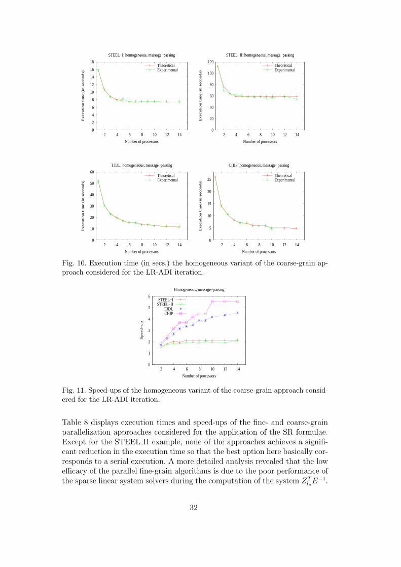
Figure 10 compares the theoretical and experimental execution times (seeequations (18) and (19)) of the parallel homogeneous coarse-grain approachfor the four examples, as the number of processors is increased. In all fourexamples the theoretical models capture the behavior of the actual parallelcodes remarkably well. The expression in the right-hand side of equation (20)also offers the number of processors for which the minimum execution time isobtained: np ≈ 3.7, 2.8, 19.8, and 22.1 for the STEEL I, STEEL II, T3DL, andCHIP examples. This roughly corresponds to the moment the curves in thefirst two plots flatten, while, for the last two examples, not enough processorsare available to contrast this result.

Figure 11 reports the acceleration obtained in each example using the homo-geneous coarse-grain parallel code. Although the speed-ups are only moderatewhen the number of processes is large, it is necessary to realize that for theseproblems, using up to np = 14 nodes can be excessive. Indeed, the speed-upsare 1.47/1.62 for examples STEEL I/STEEL II on 2 processors, and 3.13/3.69for examples T3DL/CHIP on 5 processors, which can be considered as notable.

4.4.3 SVD

Table 7 lists the execution times and speed-ups of the parallelization of thisstage using the only option that is available: the fine-grain approach. Thetwo operations in this stage, the computation of the product Y T

lc Zlo and itsSVD, operate on dense matrices using parallel kernels from ScaLAPACK. Theoverall performance of the stage is thus determined by the parallel efficiencyof routines pdgemm and pdgesvd in this library. Again we note that the bulkof the computations here usually comes from the product Y T

lc Zlo rather thanthe small-size SVD.

4.4.4 SR formulae

In subsection 3.5 we discussed two orders in which the computation of TL

could be arranged, as TL := Σ−1/2L (V T

L ZTlo)E

−1 or TL := Σ−1/2L V T

L (ZTloE

−1). Aswe aim at partially overlapping this stage with the LR-ADI iteration, we onlyinvestigate the second choice.

31

0

2

4

6

8

10

12

14

16

18

2 4 6 8 10 12 14

Exe

cu

tio

n t

ime

(in

se

co

nd

s)

Number of processors

STEEL−I; homogeneous, message−passing

TheoreticalExperimental

0

20

40

60

80

100

120

2 4 6 8 10 12 14

Exe

cu

tio

n t

ime

(in

se

co

nd

s)

Number of processors

STEEL−II; homogeneous, message−passing

TheoreticalExperimental

0

10

20

30

40

50

60

2 4 6 8 10 12 14

Exe

cu

tio

n t

ime

(in

se

co

nd

s)

Number of processors

T3DL; homogeneous, message−passing

TheoreticalExperimental

0

5

10

15

20

25

2 4 6 8 10 12 14

Exe

cu

tio

n t

ime

(in

se

co

nd

s)

Number of processors

CHIP; homogeneous, message−passing

TheoreticalExperimental

Fig. 10. Execution time (in secs.) the homogeneous variant of the coarse-grain ap-proach considered for the LR-ADI iteration.

0

1

2

3

4

5

6

2 4 6 8 10 12 14

Sp

ee

d−

up

Number of processors

Homogeneous, message−passing

STEEL−ISTEEL−II

T3DLCHIP

Fig. 11. Speed-ups of the homogeneous variant of the coarse-grain approach consid-ered for the LR-ADI iteration.

Table 8 displays execution times and speed-ups of the fine- and coarse-grainparallelization approaches considered for the application of the SR formulae.Except for the STEEL II example, none of the approaches achieves a signifi-cant reduction in the execution time so that the best option here basically cor-responds to a serial execution. A more detailed analysis revealed that the lowefficacy of the parallel fine-grain algorithms is due to the poor performance ofthe sparse linear system solvers during the computation of the system ZT

loE−1.

32

Example Sequential Fine-grain

(1 Proc.) 2 Proc. 4 Proc. 6 Proc.

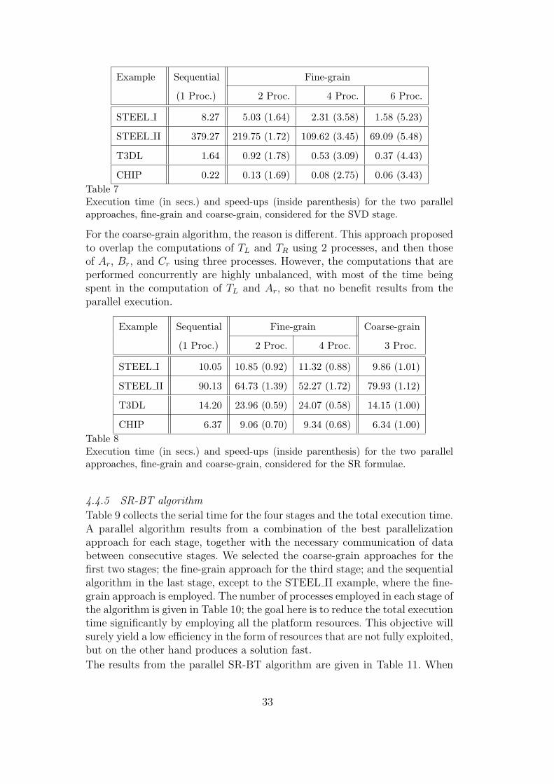
STEEL I 8.27 5.03 (1.64) 2.31 (3.58) 1.58 (5.23)

STEEL II 379.27 219.75 (1.72) 109.62 (3.45) 69.09 (5.48)

T3DL 1.64 0.92 (1.78) 0.53 (3.09) 0.37 (4.43)

CHIP 0.22 0.13 (1.69) 0.08 (2.75) 0.06 (3.43)

Table 7Execution time (in secs.) and speed-ups (inside parenthesis) for the two parallelapproaches, fine-grain and coarse-grain, considered for the SVD stage.

For the coarse-grain algorithm, the reason is different. This approach proposedto overlap the computations of TL and TR using 2 processes, and then thoseof Ar, Br, and Cr using three processes. However, the computations that areperformed concurrently are highly unbalanced, with most of the time beingspent in the computation of TL and Ar, so that no benefit results from theparallel execution.

Example Sequential Fine-grain Coarse-grain

(1 Proc.) 2 Proc. 4 Proc. 3 Proc.

STEEL I 10.05 10.85 (0.92) 11.32 (0.88) 9.86 (1.01)

STEEL II 90.13 64.73 (1.39) 52.27 (1.72) 79.93 (1.12)

T3DL 14.20 23.96 (0.59) 24.07 (0.58) 14.15 (1.00)

CHIP 6.37 9.06 (0.70) 9.34 (0.68) 6.34 (1.00)

Table 8Execution time (in secs.) and speed-ups (inside parenthesis) for the two parallelapproaches, fine-grain and coarse-grain, considered for the SR formulae.

4.4.5 SR-BT algorithm

Table 9 collects the serial time for the four stages and the total execution time.A parallel algorithm results from a combination of the best parallelizationapproach for each stage, together with the necessary communication of databetween consecutive stages. We selected the coarse-grain approaches for thefirst two stages; the fine-grain approach for the third stage; and the sequentialalgorithm in the last stage, except to the STEEL II example, where the fine-grain approach is employed. The number of processes employed in each stage ofthe algorithm is given in Table 10; the goal here is to reduce the total executiontime significantly by employing all the platform resources. This objective willsurely yield a low efficiency in the form of resources that are not fully exploited,but on the other hand produces a solution fast.

The results from the parallel SR-BT algorithm are given in Table 11. When

33

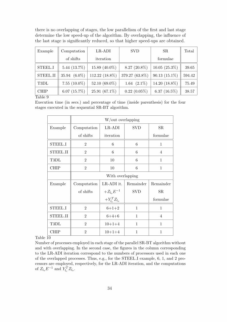
there is no overlapping of stages, the low parallelism of the first and last stagedetermine the low speed-up of the algorithm. By overlapping, the influence ofthe last stage is significantly reduced, so that higher speed-ups are obtained.

Example Computation LR-ADI SVD SR Total

of shifts iteration formulae

STEEL I 5.44 (13.7%) 15.89 (40.0%) 8.27 (20.8%) 10.05 (25.3%) 39.65

STEEL II 35.94 (6.0%) 112.22 (18.8%) 379.27 (63.8%) 90.13 (15.1%) 594.42

T3DL 7.55 (10.0%) 52.10 (69.0%) 1.64 (2.1%) 14.20 (18.8%) 75.49

CHIP 6.07 (15.7%) 25.91 (67.1%) 0.22 (0.05%) 6.37 (16.5%) 38.57

Table 9Execution time (in secs.) and percentage of time (inside parenthesis) for the fourstages executed in the sequential SR-BT algorithm.

W/out overlapping

Example Computation LR-ADI SVD SR

of shifts iteration formulae

STEEL I 2 6 6 1

STEEL II 2 6 6 4

T3DL 2 10 6 1

CHIP 2 10 6 1

With overlapping

Example Computation LR-ADI it. Remainder Remainder

of shifts +ZloE−1 SVD SR

+Y Tlc

Zlo formulae

STEEL I 2 6+1+2 1 1

STEEL II 2 6+4+6 1 4

T3DL 2 10+1+4 1 1

CHIP 2 10+1+4 1 1

Table 10Number of processes employed in each stage of the parallel SR-BT algorithm withoutand with overlapping. In the second case, the figures in the column correspondingto the LR-ADI iteration correspond to the numbers of processors used in each oneof the overlapped processes. Thus, e.g., for the STEEL I example, 6, 1, and 2 pro-cessors are employed, respectively, for the LR-ADI iteration, and the computationsof ZloE

−1 and Y Tlc

Zlo .

34

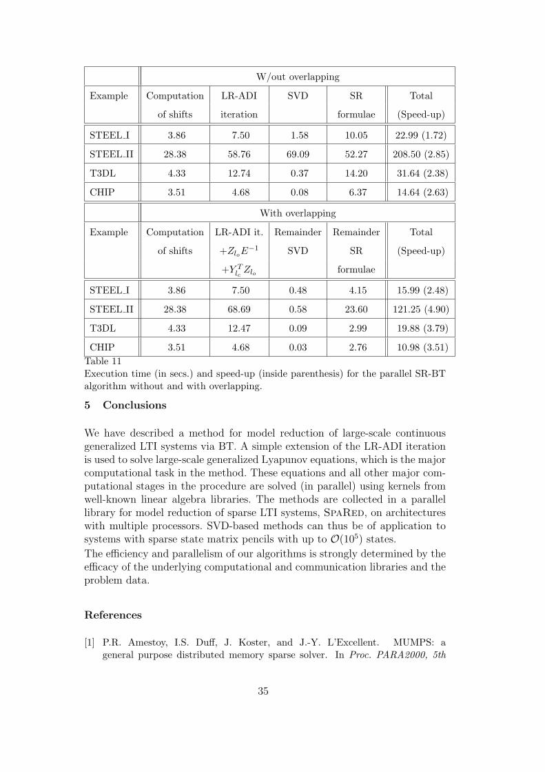
W/out overlapping

Example Computation LR-ADI SVD SR Total

of shifts iteration formulae (Speed-up)

STEEL I 3.86 7.50 1.58 10.05 22.99 (1.72)

STEEL II 28.38 58.76 69.09 52.27 208.50 (2.85)

T3DL 4.33 12.74 0.37 14.20 31.64 (2.38)

CHIP 3.51 4.68 0.08 6.37 14.64 (2.63)

With overlapping

Example Computation LR-ADI it. Remainder Remainder Total

of shifts +ZloE−1 SVD SR (Speed-up)

+Y Tlc

Zlo formulae

STEEL I 3.86 7.50 0.48 4.15 15.99 (2.48)

STEEL II 28.38 68.69 0.58 23.60 121.25 (4.90)

T3DL 4.33 12.47 0.09 2.99 19.88 (3.79)

CHIP 3.51 4.68 0.03 2.76 10.98 (3.51)

Table 11Execution time (in secs.) and speed-up (inside parenthesis) for the parallel SR-BTalgorithm without and with overlapping.

5 Conclusions

We have described a method for model reduction of large-scale continuousgeneralized LTI systems via BT. A simple extension of the LR-ADI iterationis used to solve large-scale generalized Lyapunov equations, which is the majorcomputational task in the method. These equations and all other major com-putational stages in the procedure are solved (in parallel) using kernels fromwell-known linear algebra libraries. The methods are collected in a parallellibrary for model reduction of sparse LTI systems, SpaRed, on architectureswith multiple processors. SVD-based methods can thus be of application tosystems with sparse state matrix pencils with up to O(105) states.

The efficiency and parallelism of our algorithms is strongly determined by theefficacy of the underlying computational and communication libraries and theproblem data.

References

[1] P.R. Amestoy, I.S. Duff, J. Koster, and J.-Y. L’Excellent. MUMPS: ageneral purpose distributed memory sparse solver. In Proc. PARA2000, 5th

35

International Workshop on Applied Parallel Computing, pages 122–131, 2000.

[2] A.C. Antoulas. Approximation of Large-Scale Dynamical Systems. SIAMPublications, Philadelphia, PA, 2005.

[3] J. M. Badıa, P. Benner, R. Mayo, and E. S. Quintana-Ortı. Parallel algorithmsfor balanced truncation model reduction of sparse systems. In J. Dongarra,K. Madsen, and J. Wasniewski, editors, Applied Parallel Computing: 7th

International Conference, PARA 2004, Lyngby, Denmark, June 20-23, 2004.

Revised Selected Papers, volume 3732 of Lecture Notes in Computer Science,pages 267–275. Springer-Verlag, Berlin, Heidelberg, New York, 2006.

[4] R.H. Bartels and G.W. Stewart. Solution of the matrix equation AX+XB = C:Algorithm 432. Comm. ACM, 15:820–826, 1972.

[5] U. Baur and P. Benner. Factorized solution of Lyapunov equations based onhierarchical matrix arithmetic. Computing, to appear.

[6] P. Benner. Solving large-scale control problems. IEEE Control Systems

Magazine, 14(1):44–59, 2004.

[7] P. Benner, V. Mehrmann, and D.C. Sorensen, editors. Dimension Reduction of

Large-Scale Systems, volume 45 of Lecture Notes in Computational Science and

Engineering. Springer-Verlag, Berlin/Heidelberg, Germany, 2005.

[8] P. Benner, H. Mena, and J. Saak. On the parameter section problem in theNewton-ADI iteration for large scale riccati equations. Preprint, Fakultat furMathematik, TU Chemnitz, D-09107 Chemnitz, Germany, October 2006.

[9] P. Benner, E.S. Quintana-Ortı, and G. Quintana-Ortı. Balanced truncationmodel reduction of large-scale dense systems on parallel computers. Math.

Comput. Model. Dyn. Syst., 6(4):383–405, 2000.

[10] P. Benner, E.S. Quintana-Ortı, and G. Quintana-Ortı. State-space truncationmethods for parallel model reduction of large-scale systems. Parallel Comput.,29:1701–1722, 2003.

[11] P. Benner and J. Saak. A semi-discretized heat transfer model for optimalcooling of steel profiles. Chapter 19 (pages 353–356) of [7].

[12] L.S. Blackford, J. Choi, A. Cleary, E. D’Azevedo, J. Demmel, I. Dhillon,J. Dongarra, S. Hammarling, G. Henry, A. Petitet, K. Stanley, D. Walker, andR.C. Whaley. ScaLAPACK Users’ Guide. SIAM, Philadelphia, PA, 1997.

[13] Y. Chahlaoui and P. Van Dooren. A collection of benchmark examples formodel reduction of linear time invariant dynamical systems. SLICOT WorkingNote 2002–2, February 2002. Available from www.slicot.org.

[14] J.W. Demmel, J.R. Gilbert, and X.S. Li. SuperLU Users’ Guide.

[15] G.H. Golub and C.F. Van Loan. Matrix Computations. Johns HopkinsUniversity Press, Baltimore, third edition, 1996.

36

[16] S. Gugercin and J.-R. Li. Smith-type methods for balanced truncation of largesystems. Chapter 2 (pages 49–82) of [7].

[17] S. Gugercin, D.C. Sorensen, and A.C. Antoulas. A modified low-rank Smithmethod for large-scale Lyapunov equations. Numer. Algorithms, 32(1):27–55,2003.

[18] S.J. Hammarling. Numerical solution of the stable, non-negative definiteLyapunov equation. IMA J. Numer. Anal., 2:303–323, 1982.

[19] J.-R. Li and T. Penzl. Square root method via Cholesky factor ADI. In Proc.

MTNS 2000, Perpignan, 2000. (CD Rom).

[20] J.-R. Li and J. White. Low rank solution of Lyapunov equations. SIAM J.

Matrix Anal. Appl., 24(1):260–280, 2002.

[21] J. Lienemann, E. B. Rudnyi, and J. G. Korvink. MST MEMS model orderreduction: Requirements and benchmarks. Linear Algebra Appl., 415(2–3):469–498, 2006.

[22] B.C. Moore. Principal component analysis in linear systems: Controllability,observability, and model reduction. IEEE Trans. Automat. Control, AC-26:17–32, 1981.

[23] G. Obinata and B.D.O. Anderson. Model Reduction for Control System Design.Communications and Control Engineering Series. Springer-Verlag, London, UK,2001.

[24] T. Penzl. A cyclic low rank Smith method for large sparse Lyapunov equations.SIAM J. Sci. Comput., 21(4):1401–1418, 2000.

[25] T. Penzl. Lyapack Users Guide. Technical Report SFB393/00-33,Sonderforschungsbereich 393 Numerische Simulation auf massiv parallelen

Rechnern, TU Chemnitz, 09107 Chemnitz, FRG, 2000. Available from http:

//www.tu-chemnitz.de/sfb393/sfb00pr.html.

[26] T. Penzl. Algorithms for model reduction of large dynamical systems.Linear Algebra Appl., 415(2–3):322–343, 2006. (Reprint of Technical ReportSFB393/99-40, TU Chemnitz, 1999.).

[27] G. Quintana-Ortı, X. Sun, and C.H. Bischof. A BLAS-3 version of the QRfactorization with column pivoting. SIAM J. Sci. Comput., 19:1486–1494, 1998.

[28] M.G. Safonov and R.Y. Chiang. A Schur method for balanced-truncation modelreduction. IEEE Trans. Automat. Control, AC–34:729–733, 1989.

[29] T. Stykel. Gramian-based model reduction for descriptor systems. Math.

Control, Signals, Sys., 16:297–319, 2004.

[30] T. Stykel. Low rank iterative methods for projected generalized Lyapunovequations. Preprint 198, DFG Research Center Matheon, TU Berlin, 2005.Available from http://www.math.tu-berlin.de/∼stykel/Publications/pr

04 198.pdf.

37

[31] F. Troltzsch and A. Unger. Fast solution of optimal control problems in theselective cooling of steel. Z. Angew. Math. Mech., 81:447–456, 2001.

[32] R.A. van de Geijn. Using PLAPACK: Parallel Linear Algebra Package. MITPress, Cambridge, MA, 1997.

[33] A. Varga. Efficient minimal realization procedure based on balancing. InPrepr. of the IMACS Symp. on Modelling and Control of Technological Systems,volume 2, pages 42–47, 1991.

[34] A. Varga. Model reduction software in the SLICOT library. In B.N. Datta,editor, Applied and Computational Control, Signals, and Circuits, volume 629of The Kluwer International Series in Engineering and Computer Science, pages239–282. Kluwer Academic Publishers, Boston, MA, 2001.

[35] E.L. Wachspress. ADI iteration parameters for the Sylvester equation, 2000.Available from the author.

38

Chemnitz Scientific Computing Preprints – ISSN 1864-0087