balance and filtering in structured satisfiability problems

Balance and Filtering in Structured Satisfiability Problems

Henry Kautz

University of Washingtonjoint work with

Yongshao Ruan (UW), Dimitris Achlioptas (MSR), Carla Gomes (Cornell), Bart Selman (Cornell),

Mark Stickel (SRI)

CORE – UW, MSR, Cornell

Speedup Learning Machine learning historically considered

Learning to classify objects Learning to search or reason more efficiently

Speedup Learning Speedup learning disappeared in mid-90’s

Last workshop in 1993 Last thesis 1998

What happened? EBL (without generalization) “solved”

rel_sat (Bayardo), GRASP (Silva 1998), Chaff (Malik 2001) – 1,000,000 variable verification problems

EBG too hard algorithmic advances outpaced any successes

Alternative Path

Predictive control of search and reasoning Learn statistical model of behavior of a problem solver

on a problem distribution Use the model as part of a control strategy to improve

the future performance of the solver Synthesis of ideas from

Phase transition phenomena in problem distributions Decision-theoretic control of reasoning Bayesian modeling

Big Picture

ProblemInstances

Solver

static features

runtime

Learning /Analysis

PredictiveModel

dynamic features

resource allocation / reformulation

control / policy

Case Study: Beyond 4.25

ProblemInstances

Solver

static features

runtime

Learning /Analysis

PredictiveModel

Phase transitions & problem hardness

Large and growing literature on random problem distributions

Peak in problem hardness associated with critical value of some underlying parameter

3-SAT: clause/variable ratio = 4.25 Using measured parameter to predict hardness of

a particular instance problematic! Random distribution must be a good model of actual

domain of concern Recent progress on more realistic random

distributions...

Quasigroup Completion Problem (QCP)

NP-Complete Has structure is similar to that of real-world problems -

tournament scheduling, classroom assignment, fiber optic routing, experiment design, ...

Start with empty grad, place colors randomly Generates mix of sat and unsat instances

Phase Transition

Almost all unsolvable area

Fraction of pre-assignment

Fra

ctio

n o

f u

nso

lvab

le c

ases

Almost all solvable area

Complexity Graph

Phase transition

42% 50%20%

42% 50%20%

Underconstrained area

Critically constrained area

Overconstrained area

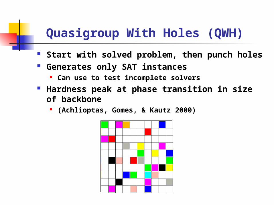
Quasigroup With Holes (QWH)

Start with solved problem, then punch holes Generates only SAT instances

Can use to test incomplete solvers Hardness peak at phase transition in size of

backbone (Achlioptas, Gomes, & Kautz 2000)

New Phase Transition in Backbone

% Backbone

% holes

Computationalcost%

of

Bac

kbo

ne

Easy-Hard-Easy pattern in local search

% holes

Co

mp

uta

tio

na

l Co

st

WalksatOrder 30, 33, 36

“Over” constrained area

Underconstrained area

Are we ready to predict run times?

Problem: high variance

1.E+00

1.E+01

1.E+02

1.E+03

1.E+04

1.E+05

1.E+06

1.E+07

1.E+08

1.E+09

0.2 0.25 0.3 0.35 0.4 0.45 0.5

log scale

Deep structural features

Rectangular Pattern(Hall 1945)

Aligned Patternnew result!

Balanced Pattern

Tractable Very hard

Hardness is also controlled by structure of constraints, not just the fraction of holes

Random versus balanced

BalancedRandom

Random versus balanced

0.E+00

1.E+07

2.E+07

3.E+07

4.E+07

5.E+07

6.E+07

7.E+07

0.2 0.25 0.3 0.35 0.4 0.45 0.5

Balanced

Random

Random vs. balanced (log scale)

1.E+00

1.E+01

1.E+02

1.E+03

1.E+04

1.E+05

1.E+06

1.E+07

1.E+08

1.E+09

0.2 0.25 0.3 0.35 0.4 0.45 0.5

Balanced

Random

Morphing balanced and random

Mixed Model - Walksat

0

10

20

30

40

50

60

70

80

90

100

0.00% 20.00% 40.00% 60.00% 80.00% 100.00%

Percent random holes

Tim

e (s

econds)

order 33

Considering variance in hole pattern


0

10

20

30

40

50

60

70

80

90

100

0 2 4 6 8

variance in # holes / row

tim

e

order 33

Time on log scale


1

10

100

0 2 4 6 8

variance in # holes / row

tim

e (s

econds)

log s

cale

order 33

Balanced patterns yield (on average) problems that are 2 orders of magnitude harder than random patterns

Expected run time decreases exponentially with variance in # holes per row or column

Same pattern (differ constants) for DPPL! At extreme of high variance (aligned model) can

prove no hard problems exist

Effect of balance on hardness

2

( ) kE T C

0.1

1

10

0 10 20 30 40 50

variance

tim

e (

se

co

nd

s)

Morphing random and rectangular

order 36

0.01

0.1

1

10

0 50 100 150 200 250 300

variance in # holes

tim

e (

se

co

nd

s)

Morphing random and rectangular

order 33

artifact of walksatartifact of walksat

Morphing Balanced Random Rectangular

0.1

1

10

100

0 5 10 15 20

variance

tim

e (

se

co

nd

s)

order 33

Intuitions

In unbalanced problems it is easier to identify most critically constrained variables, and set them correctly

Backbone variables

Are we done?

Not yet... Observation 1: While few unbalanced problems

are hard, quite a few balanced problems are easy To do: find additional structural features that

predict hardness Introspection Machine learning (Horvitz et al. UAI 2001) Ultimate goal: accurate, inexpensive prediction of

hardness of real-world problems

Are we done?

Not yet… Observation 2: Significant differences in the SAT

instances in hardest regions for the QCP and QWH generators

QWH

QCP(sat only)

Biases in Generators

An unbiased SAT-only generator would sample uniformly at random from the space of all SAT CSP problems

Practical CSP generators Incremental arc-consistency introduces dependencies Hard to formally model the distribution

QWH generator Clean formal model Slightly biased toward problems with many solutions Adding balance makes small, hard problems

balanced QCP balanced QWH

random QCP random QWH

1.E+00

1.E+01

1.E+02

1.E+03

1.E+04

1.E+05

1.E+06

1.E+07

1.E+08

1.E+09

0.2 0.25 0.3 0.35 0.4 0.45 0.5

% holes

flip

s

Conclusions

One small part of an exciting direction for improving power of search and reasoning algorithms

Hardness prediction can be used to control solver policy

Noise level (Patterson & Kautz 2001) Restarts (Horvitz et al (CORE team ) UAI 2001)

Lots of opportunities for cross-disciplinary work Theory Machine learning Experimental AI and OR Reasoning under uncertainty Statistical physics

balance and filtering in structured satisfiability problems

Documents