bai giai truyen thong khong day moi

of 246

Chapter 2Problem 1 Powerlawprofiles.mclear%powerlawprofiles.m; calculates the powerloss as per inverse square law and 1/d^n.close allnu=[2 3 3.5 4];%four values of the loss parameterfor k=1:4; n=nu(k);d=1:50;% distance in Kmd1=d.^n;dn=1./d1;pn=-10.*log10(dn);%inverse lawplot(d,pn,'k');xlabel('distance in Km');ylabel('powerloss in dB');hold onend;

of 246

Problem 2 From the book, eqn. (2.2) is2 2

2 2 2

1000 2 116 16 3 5000

r r td

P G GPL d

.

The wavelength 13

m . 85.6 10 72.5dP dBm .

Problem 3& 4 hataloss.m

clear% hataloss.m Power loss calculationscarf=input('enter carrier freq. in MHZ...>>');lcrf=log10(carf);ht=input('enter the height of BS antenna in meters..>>');%height in meters of the BSlht=log10(ht);hr=input('enter the height of the MU antenna in meters..>>');%MU ant. height in meterslhr=log10(11.75*hr);N=60;%number of increments for distancedistmax=30;%coverage distance in Kmsfor kk=1:1:59;d(kk)=1+0.5*(kk-1);fact1=69.55+26.16*lcrf-13.83*lht;fact2=(44.9-6.55*lht)*log10(d(kk));fftq=fact1+fact2;%antenna correction factor MU...ahr=3.2*(lhr)^2-4.97;% large cities; freq. above 400 MHzamr=(1.1*lcrf-0.7)*hr-(1.56*lcrf-0.8);alar(kk)=fftq-ahr;amed(kk)=fftq-amr;asub(kk)=amed(kk)-2*(log10(carf/28)).^2-5.4;arur(kk)=amed(kk)-4.78*(lcrf.^2)+18.33*lcrf-40.94;end;

subplot(2,2,1); plot(d,alar); xlabel('distance Km'); ylabel('power loss dB'); title('large city');

subplot(2,2,2); plot(d,amed);

%axis([1 30 -140 -60]); xlabel('distance Km'); ylabel('power loss dB'); title('medium city');

subplot(2,2,3);

of 246

plot(d,asub);

%axis([1 30 -140 -60]); xlabel('distance Km'); ylabel('power loss dB'); title('suburban');

subplot(2,2,4); plot(d,arur);

%axis([1 30 -140 -60]); xlabel('distance Km'); ylabel('power loss dB'); title('rural');

%loss at a reference distance of 100 m Wave=3e8/900e6;%wavelength in meters PL=10*log10((4*pi*100)^2/Wave^2);%relative loss at 100 meters d3=d(3)*1000;%distance in meters %use eqn. (2.19) denom=10*log10(d3/100);%denominator of eqn. (2.19) nuLarge=(alar(3)-PL)/denom%nu for large city nuMed=(amed(3)-PL)/denom%nu for med city nuSub=(asub(3)-PL)/denom%nu for suburbs city nuRur=(arur(3)-PL)/denom%nu for rural city

of 246

Large = 4.1865Med = 4.1801Sub =3.4159Rur =1.9890

Problem 5.fadcom.m

clear%fadcom.m simulates Doppler fading including a carrier frequency and then demodulate%uses random phase model for both Rayleigh and Rician fading% also computes the outage probabilityfc=900e3;%carrier frequencyppf=2*pi*fc;N=11;% Number of mutiple pathsfd=input('enter the Doppler shift...')ppw=2*pi*fd;%scattering strengths are considered to be Gamma distributed

of 246

fs=4*fc;%sampling rateTs=1/fs;t = [0:Ts:1999*Ts]; %time arraynn=length(t);ci=zeros(1,nn); %received signal (Rayleigh for m=1:N; a = gamrnd(1.4,1,1,nn); ppwt=ppw*unifrnd(0,2*pi,1,nn); ci = ci + a.*cos((ppf+ppwt).*t+ppwt+unifrnd(0,2*pi,1,nn));end;cr=ci;crr=ci+2*cos(ppf*t);%generates Rician[x,y]=demod(cr,fc,fs,'qam');[xr,yr]=demod(crr,fc,fs,'qam');ae=(1/N)*sqrt(x.^2+y.^2);aer=(1/N)*sqrt(xr.^2+yr.^2); pha=pi+angle(x+i*y);%phase to be centered around 2*pi figuresubplot(2,1,1)plot(t*1e3,cr),title('Rayleigh fading')xlabel('time ms')ylabel('rf signal volt')xlim([0 .1])aes=20*log10(ae);subplot(2,1,2)plot(t*1e3,aes),title('Rayleigh fading')xlabel('time ms')ylabel('relative power dB')xlim([0 .1])figuresubplot(2,1,1)plot(t*1e3,crr),title('Rician fading')xlabel('time ms')ylabel('rf signal volt')xlim([0 .1])

aerr=20*log10(aer);

subplot(2,1,2)plot(t*1e3,aerr),title('Rician fading')xlabel('time ms')ylabel('relative power dB')xlim([0 .1])

fractra=0.0;for mf=1:nn;

of 246

if aes(mf)<=-10 fractra=fractra+1; else end;end;outageRayl=fractra/nnfractrc=0.0;for mf=1:nn; if aerr(mf)<=-10 fractrc=fractrc+1; else end;end;outageRice=fractrc/nn

Problem 6.fadingsim.m

of 246

clear%fadingsim.m simulates fading including a carrier frequency and then demodulate%uses random phase model as well as random delayfc=900e3;%carrier frequencyppf=2*pi*fc;N=11;% Number of mutiple paths%a are considered to be Gamma distributedfs=4*fc;%sampling rate

Ts=1/fs;t = [0:Ts:1999*Ts]; %time arraynn=length(t);ci=zeros(1,nn); %received signal (Rayleighnn=length(t);dist=1000;%distance between transmit and receive in metersavdel=dist/3e8%average delay in seconds ci=zeros(1,nn); cir=zeros(1,nn); cit=0.0;%this uses a delay instead of Uniform phase for m=1:N; phterm=unifrnd(0,2*pi,1,nn); delay=avdel+(-0.5+unifrnd(0,2*pi,1,nn))*avdel;%uniform delay with a mean of avdel a = gamrnd(1.4,1,1,nn); ci=ci+a.*cos(ppf*t+phterm);%Rayleigh %following term generates the received signal with delay format cit=cit+a.*cos(ppf*t+delay); end;crr=cit+2*cos(ppf*t);%rician[x,y]=demod(ci,fc,fs,'qam');[xt,yt]=demod(cit,fc,fs,'qam');[xr,yr]=demod(crr,fc,fs,'qam');ae=(1/N)*sqrt(x.^2+y.^2);aet=(1/N)*sqrt(xt.^2+yt.^2);aer=(1/N)*sqrt(xr.^2+yr.^2);

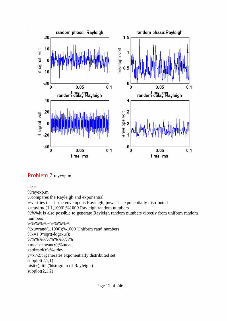
pha=pi+angle(x+i*y);%phase to be centered around 2*pi phat=pi+angle(xt+i*yt);%phase of the delay versionfiguresubplot(2,2,1)plot(t*1e3,ci),title('random phase: Rayleigh');xlabel('time ms')ylabel('rf signal volt')xlim([0 0.1])

subplot(2,2,2)

of 246

plot(t*1e3,ae),title('random phase:Rayleigh');xlabel('time ms')ylabel('envelope volt')xlim([0 0.1])

subplot(2,2,3)plot(t*1e3,cit),title('random delay:Rayleigh');xlabel('time ms')ylabel('rf signal volt')xlim([0 0.1])

subplot(2,2,4)plot(t*1e3,aet),title('random delay:Rayleigh');xlabel('time ms')ylabel('envelope volt')xlim([0 0.1])

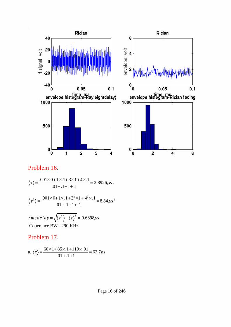
figuresubplot(2,2,1)plot(t*1e3,crr),title('Rician')xlabel('time ms')ylabel('rf signal volt')xlim([0 0.1])

subplot(2,2,2)plot(t*1e3,aer),title('Rician')xlabel('time ms')ylabel('envelope volt')xlim([0 0.1])

subplot(2,2,4)hist(aer),title('envelope histogram-Rician fading')

subplot(2,2,3);hist(aet),title('envelope histogram-Rayleigh(delay)')

of 246

Problem 7.rayexp.m

clear%rayexp.m%compares the Rayleigh and exponential%verifies that if the envelope is Rayleigh, power is exponentially distributedx=raylrnd(1,1,1000);%1000 Rayleigh random numbers%%%It is also possible to generate Rayleigh random numbers directly from uniform randomnumbers%%%%%%%%%%%%xu=rand(1,1000);%1000 Uniform rand numbers%x=1.0*sqrt(-log(xu));%%%%%%%%%%%%xmean=mean(x);%meanxstd=std(x);%stdevy=x.^2;%generates exponentially distributed setsubplot(2,1,1)hist(x),title('histogram of Rayleigh')subplot(2,1,2)

of 246

hist(y),title('histogram of exponential');ymean=mean(y)ystd=std(y)ratio_Rayl=xmean/xstdratio_exp=ymean/ystdratio_Rayl=xmean/xstdratio_exp=ymean/ystd

ratio_Rayl = 1.8818ratio_exp = 0.9684

Problem 8.fadcom

outageRayl =

0.2945

Problem 9.fadcom

of 246

Problem 10.fadcom.moutageRayl =

0.2945

outageRice =

0.2500

Problem 11. If the signal is Rayleigh faded, the power is exponentially distributed.

Therefore, the outage probability Pout is given by0

1 exp Tout

ZP

Z

where Z0 is the average power and ZT is the threshold power.

Z0 =10 dBm 10 mW

of 246

ZT=0 dBm 1 mW

Outage Probability = 11 exp 0.27110

.

Problem 121Prob SNR<0dB 1 exp2

= 03935.

Problem 13. Threshold = 25-10=15 dB or 101.5.

Mean SNR = 25 dB or 102.5.1.5

2.5

101 exp 0.0952

10outP .

Problem 14. Threshold = 5 dB or 10.5.

.5

0

100.02 1 expoutP

Z where Z0 is the average SNR.

.5

010 156.5 22

log .98e

Z dB

Problem 15. fadingsim.m

of 246

Problem 16.

.001 0 1 .1 3 1 4 .1 2.8926.01 .1 1 .1

s .

2 22 2.001 0 1 .1 3 1 4 .1 8.84

.01 .1 1 .1s

22. . 0.6898rmsdelay s

Coherence BW =290 KHz.

Problem 17.

a. 60 1 85 .1 110 .01 62.7.01 .1 1

ns

of 246

2 2 22 260 1 85 .1 110 .01 4000

.01 .1 1ns

22. . 8.48rmsdelay ns

b.

0 .01 4 .1 8 1 7.57.01 .1 1

s

2 2 22 20 .01 4 .1 8 1 59.1

.01 .1 1s

22. . 1.36rmsdelay s

The response represented by (a) is an indoor channel response while the response represented by(b) is an outdoor channel one.

Problem 18. hatalog.m

clear% hatalog.m Power loss calculations%incluse a plot of the lognormal fading suprimposedclose allPt=30;%power in dBm transmitted 1Wcarf=input('enter carrier freq. in MHZ...>>');lcrf=log10(carf);ht=input('enter the height of BS antenna in meters..>>');%height in meters of the BSlht=log10(ht);hr=input('enter the height of the MU antenna in meters..>>');%MU ant. height in meterslhr=log10(11.75*hr);N=60;%number of increments for distancedistmax=30;%coverage distance in Kmsfor kk=1:1:39;d(kk)=1+0.5*(kk-1);fact1=69.55+26.16*lcrf-13.83*lht;fact2=(44.9-6.55*lht)*log10(d(kk));fftq=fact1+fact2;%antenna correction factor MU...ahr=3.2*(lhr)^2-4.97;% large cities; freq. above 400 MHzamr=(1.1*lcrf-0.7)*hr-(1.56*lcrf-0.8);alar(kk)=Pt-(fftq-ahr);

of 246

amed(kk)=Pt-(fftq-amr);asub(kk)=Pt-(fftq-ahr-2*(log10(carf/28)).^2-5.4);arur(kk)=Pt-(fftq-ahr-4.78*(lcrf.^2)+18.33*lcrf-40.94);xlar(kk)=alar(kk)+normrnd(0,10);%10 dB std deviation for big city with mean equal to thereceived powerxmed(kk)=amed(kk)+normrnd(0,8);%8 dB std deviation for med cityxsub(kk)=asub(kk)+normrnd(0,4);%4 dB std deviationxrur(kk)=arur(kk)+normrnd(0,3);%3 dB std deviation

end;

subplot(2,2,1) plot(d,alar,d,xlar); xlabel('distance Km'); xlim([2 20]) ylabel('Received Power dBm'); title('large city');

subplot(2,2,2) plot(d,amed,d,xmed);

%axis([1 30 -140 -60]); xlabel('distance Km'); xlim([2 20]) ylabel('Received Power dBm'); title('medium city');

subplot(2,2,3) plot(d,asub,d,xsub);

%axis([1 30 -140 -60]); xlabel('distance Km'); xlim([2 20]) ylabel('Received Power dBm'); title('suburban');

subplot(2,2,4) plot(d,arur,d,xrur);

%axis([1 30 -140 -60]); xlabel('distance Km'); xlim([2 20])

of 246

ylabel('Received Power dBm'); title('rural');

Problem 19. rice.m

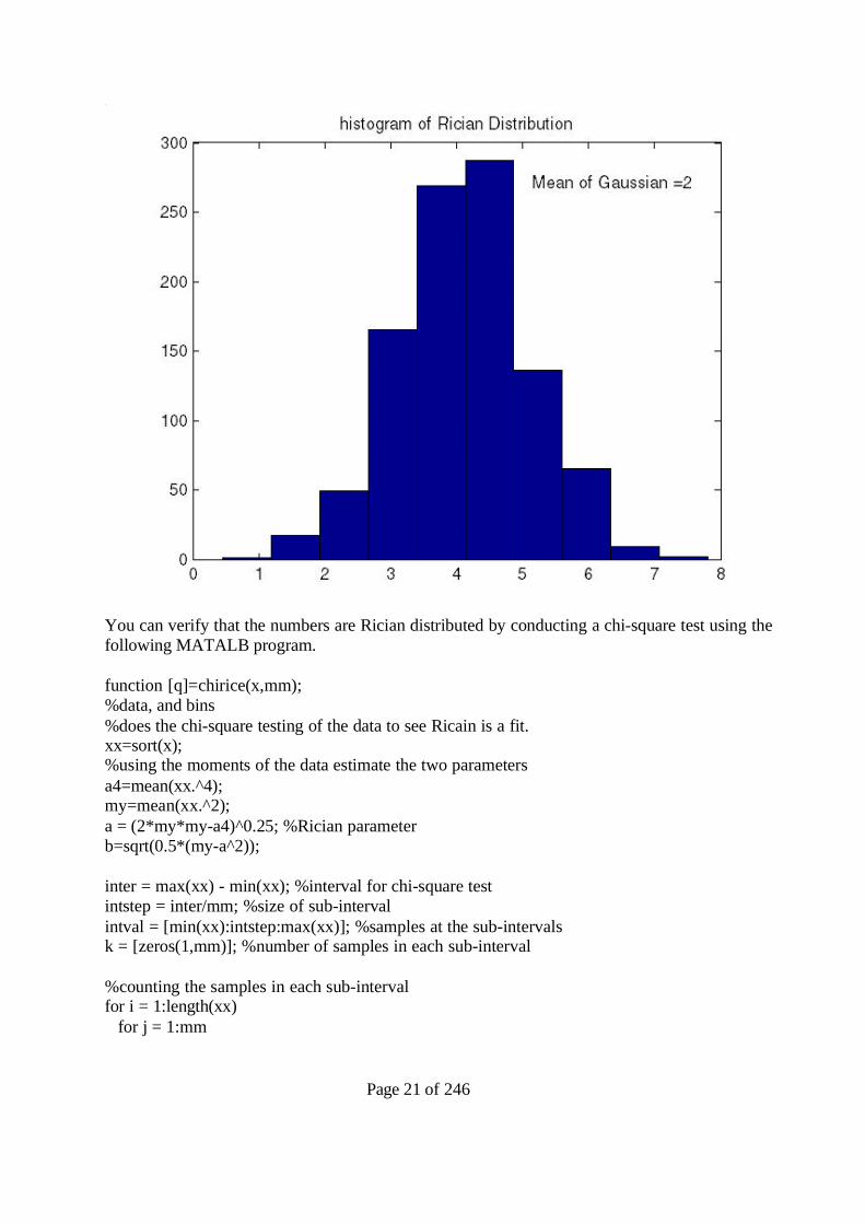
clear;close all%rice.m%generates a Rician distributionfor kr=1:10rpara=input('mean of the Gaussian to create Rician...>');rp2=rpara^2;n=1000;%number of samplesx=normrnd(0,1,1,1000);xx=normrnd(rpara,1,1,1000);ac=x.^2+xx.^2;r=sqrt(ac);%rician variable

ax=0.:0.2:20;% range of values for the histogramfigure

of 246

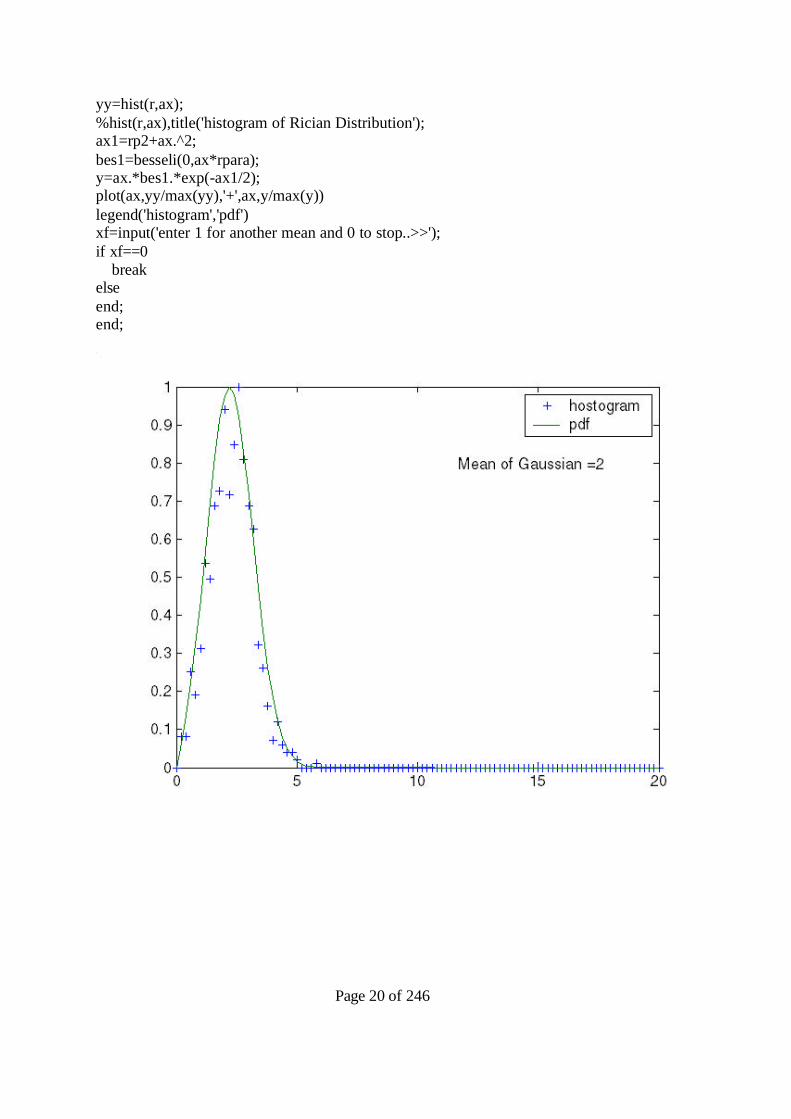
yy=hist(r,ax);%hist(r,ax),title('histogram of Rician Distribution');ax1=rp2+ax.^2;bes1=besseli(0,ax*rpara);y=ax.*bes1.*exp(-ax1/2);plot(ax,yy/max(yy),'+',ax,y/max(y))legend('histogram','pdf')xf=input('enter 1 for another mean and 0 to stop..>>');if xf==0 breakelseend;end;

of 246

You can verify that the numbers are Rician distributed by conducting a chi-square test using thefollowing MATALB program.

function [q]=chirice(x,mm);%data, and bins%does the chi-square testing of the data to see Ricain is a fit.xx=sort(x);%using the moments of the data estimate the two parametersa4=mean(xx.^4);my=mean(xx.^2);a = (2*my*my-a4)^0.25; %Rician parameterb=sqrt(0.5*(my-a^2));

inter = max(xx) - min(xx); %interval for chi-square testintstep = inter/mm; %size of sub-intervalintval = [min(xx):intstep:max(xx)]; %samples at the sub-intervalsk = [zeros(1,mm)]; %number of samples in each sub-interval

%counting the samples in each sub-intervalfor i = 1:length(xx) for j = 1:mm

of 246

if xx(i) <= intval(j+1) k(j) = k(j) + 1; break; end; end;end;Fy=1-marcumq(a/b,intval/b);%CDF uses marcumq function from Communications Toolboxp = zeros(1,mm);for i = 1:mm p(i) = Fy(i+1) - Fy(i); %probabilities at the sub-interval samplesend;

np = p.*length(xx);

q = 0;for i = 1:mm q = q + ((k(i)-np(i))^2)/np(i); %chi-square testend;

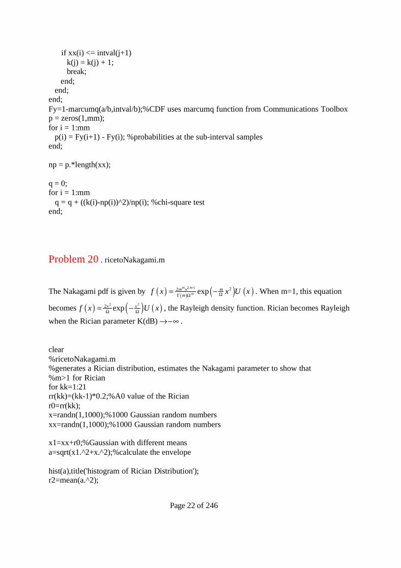
Problem 20 . ricetoNakagami.m

The Nakagami pdf is given by 2 1 22 expm m

mm x m

mf x x U x . When m=1, this equation

becomes 2 22 expx xf x U x , the Rayleigh density function. Rician becomes Rayleighwhen the Rician parameter K(dB) .

clear%ricetoNakagami.m%generates a Rician distribution, estimates the Nakagami parameter to show that%m>1 for Ricianfor kk=1:21rr(kk)=(kk-1)*0.2;%A0 value of the Ricianr0=rr(kk);x=randn(1,1000);%1000 Gaussian random numbersxx=randn(1,1000);%1000 Gaussian random numbers

x1=xx+r0;%Gaussian with different meansa=sqrt(x1.^2+x.^2);%calculate the envelope

hist(a),title('histogram of Rician Distribution');r2=mean(a.^2);

of 246

r4=mean(a.^4);m(kk)=r2^2/(r4-r2^2);end;figure

RRdB=10*log10(rr.^2/2);plot(RRdB,m,'+')xlabel('Ricean parameter dB')ylabel('Nakagami parameter m')

Problem 21. ricetoNakagami.m

Eqn. (2.59) is 2 2

0 02 2 202exp a A aAA

Af a I

.2 2 2

02E A A …….Rician2E A ……..Nakagami

Thus, 2 202 A . Also, using the expression for m (eqn. 2.72), we can write

of 246

220

24 40 0

2 22 22 200

2

21 1 1 12 1

2

AA A

m AA

.

Note that 20

210 210log AK dB

. It is now possible to relate K(dB) to the Nakagami parameter

m. (Shown above).

Problem 22. Doppler shift 6

8

900 10 80000 66.63 10 60 60d

vf f Hzc

2 .361

2

12 .6 66.67d

eav f

e

=.0043 s

2 .362 2 66.67 .6 e 70A dN f e .

Problem 23. Coherence BW = 10 KHzData rate = 5 kbps

Data rate < coherence bandwidth Channel is flat.

Coherence Time = 100 s

Pulse duration = 1 2005000

s

Pulse duration > coherence time fast fading.

Problem 24. freqselresponse.m

The relative attenuation of the frequency components varies with the strength of the two waves.This will change the coherence bandwidth of the channel.

of 246

Figure Ex. 2-24

Problem 25.Gaussexp and chiexp

clearclose all%Gaussexp.m%generates exponential from two Gaussian random numbers%histogram is compared to the exponential pdfx1=normrnd(0,.5,1,10000);%10000 Gaussian random numbersx2=normrnd(0,.5,1,10000);%10000 Gaussian random numbersy=x1.^2+x2.^2;x=min(y):max(y)/80:max(y);hist(y,x);xh=hist(y,x);hold on%plot(x,xh/max(xh))

ymean=mean(y);

of 246

ystd=std(y);ratio=ymean/ystd

exf=exppdf(x,ymean);%generates exponential pdf having the same meanhold onexf=exf*max(xh)/max(exf);plot(x,exf,'r')legend('expoential pdf')xlabel('x')ylabel('pdf or histogram')

Problem 26.pulsedisp.m

%pulsedisp.m%shows the effect of frequency selective effects by adding ten different pulses%shifted and weighted%Gaussian pulses usedclose allclearfor kp=1:3;%plots three separate generation to show the effect of random paths and random weights%w=rand(10,1);%weights for 10 pulses

of 246

%tt=100*rand(10,1);%delay is also considered to be randomNN=1024;sigma2=200;%sigmasquarep0=500;%for p=1:NN;xx=zeros(1,NN);p=1:NN; t(p)=p; p1=p-p0; for kn=1:10; xx=xx+(1/sqrt(2*pi*sigma2))*rand(1)*exp(-(p1-100*rand(1)).^2/(2*sigma2));%10 pulsesaddedend;x1=(1/sqrt(2*pi*sigma2))*rand(1)*exp(-(p1-100*rand(1)).^2/(2*sigma2));%a single pulse xxx=xx/max(xx); x1=x1/max(x1); subplot(2,2,kp+1) plot(t,xxx); xlim([400 800]) %finds the mean and standard deviation of the Gaussian pulse xpp=sum(xxx);%denominator xp=sum(t.*xxx)/xpp;%mean......sum(pi.xi)/sum(pi) t2=t.^2; xp2=sum(t2.*xxx)/xpp;%second moment stdval=sqrt((xp2-xp^2))%standard deviationend;subplot(2,2,1)plot(t,x1),title('Transmitted Pulse') xlim([400 800]) sum2=sum(x1); xy1=sum(t.*x1)/sum2; xy2=sum(t2.*x1)/sum2;stval=sqrt(xy2-xy1^2)%standard deviation ...single pulse

of 246

r.m.s width (transmitted) = 14.1421r.m.s width (received) = 25.2188, 24.2574, 24.1377

Problem 27 (a) ricetoGaussian.m

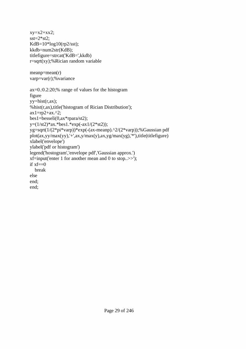
clear;close all%ricetoGaussian.m ;generates a Rician distribution%compares the histogram to Rician pdf and to a Gaussian pdf having identical%mean and variancest=2;%standared deviation of Gaussian neededst2=st^2;for kr=1:10rpara=input('mean of the Gaussian to create Rician...>');rp2=rpara^2;%use 5000 random variablesx=normrnd(0,st,1,5000);xx=normrnd(0,st,1,5000);%another gaussian random variablex1=xx+rpara;%Gaussian with different meansx2=x.^2;xx2=x1.^2;

of 246

xy=x2+xx2;sst=2*st2;KdB=10*log10(rp2/sst);kkdb=num2str(KdB);titlefigure=strcat('KdB=',kkdb)r=sqrt(xy);%Rician random variable

meanp=mean(r)varp=var(r);%variance

ax=0.:0.2:20;% range of values for the histogramfigureyy=hist(r,ax);%hist(r,ax),title('histogram of Rician Distribution');ax1=rp2+ax.^2;bes1=besseli(0,ax*rpara/st2);y=(1/st2)*ax.*bes1.*exp(-ax1/(2*st2));yg=sqrt(1/(2*pi*varp))*exp(-(ax-meanp).^2/(2*varp));%Gaussian pdfplot(ax,yy/max(yy),'+',ax,y/max(y),ax,yg/max(yg),'*'),title(titlefigure)xlabel('envelope')ylabel('pdf or histogram')legend('hostogram','envelope pdf','Gaussian approx.')xf=input('enter 1 for another mean and 0 to stop..>>');if xf==0 breakelseend;end;

of 246

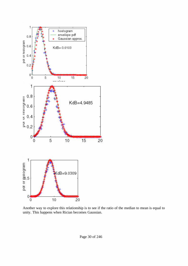
Another way to explore this relationship is to see if the ratio of the median to mean is equal tounity. This happens when Rician becomes Gaussian.

of 246

Problem 28. nakagenerice.mclear%nakagenerice.m%generates Nakagami distributed random numbers and estimates the parameters%conduct the Chi-square testing for Rayleigh and Nakagami and Rice

mval=input('enter the value of m......>');om=input('enter the value of omega....>');N=input('the number of random numbers to be generated...>');y=gamrnd(mval,om/mval,1,N);%Generates Gamma distributed random variablesx=sqrt(y);%generates Nakagami dsitributed random variable which is the square root of theGamma variablemy=mean(x.^2)%gives the value of omegaomega=myav4=mean((x.^2-my).^2);mn=my*my/av4%m-value directlymm=20;%number of binsxx=sort(x); % random samples

of 246

inter=max(x)-min(x); %interval for chi-square testintstep=inter/mm; %size of sub-intervalintval=[min(x):intstep:max(x)]; %samples at the sub-intervalsk=[zeros(1,mm)]; %number of samples in each sub-interval intializationfor i=1:N for j=1:mm if xx(i)<=intval(j+1) k(j)=k(j)+1; break; end; end;end;p=zeros(1,mm);for i=1:mm yin=intval(i+1)*intval(i+1); zin=intval(i)*intval(i); p(i)=gamcdf(yin*mn,mn,my)-gamcdf(zin*mn,mn,my); %probabilities at the sub-intervalsamplesend;np=p.*N;q=0;for i=1:mm q = q + ((k(i)-np(i))^2)/np(i); %chi-square testend;chisquare_Nakagami=q%chisquare valueq_Rayl=chirayleigh(x,mm)

if mval<=1%do not conduct the Rice test breakend;%%%% testing for Rice

%%from the paper by Nakagami%using the moments of the dataa4=mean(xx.^4);a = (2*my*my-a4)^0.25; %Rician parameterb=sqrt(0.5*(my-a^2));

inter = max(xx) - min(xx); %interval for chi-square testintstep = inter/mm; %size of sub-intervalintval = [min(xx):intstep:max(xx)]; %samples at the sub-intervalsk = [zeros(1,mm)]; %number of samples in each sub-interval

%counting the samples in each sub-intervalfor i = 1:length(xx) for j = 1:mm

of 246

if xx(i) <= intval(j+1) k(j) = k(j) + 1; break; end; end;end;

Fy=1-marcumq(a/b,intval/b);%CDF uses marcumq function from Communications Toolboxp = zeros(1,mm);for i = 1:mm p(i) = Fy(i+1) - Fy(i); %probabilities at the sub-interval samplesend;np = p.*length(xx);q = 0;for i = 1:mm q = q + ((k(i)-np(i))^2)/np(i); %chi-square testend;q_Rice=q

**The above program needs the following segment: chirayleigh

function [q]=chirayleigh(yy,m)%Tests for Rayleigh distribution%[chu)]=chirayleigh(samp,bins)y=sort(yy); % random samplesN=length(yy);my=mean(yy);%meaninter=max(y)-min(y); %interval for chi-square testintstep=inter/m; %size of sub-intervalintval=[min(y):intstep:max(y)]; %samples at the sub-intervalsk=[zeros(1,m)]; %number of samples in each sub-interval intialization

for i=1:N for j=1:m if y(i)<=intval(j+1) k(j)=k(j)+1; break; end; end;end;

myp=my*sqrt(2/pi);%Rayleigh parameterp=zeros(1,m);for i=1:m p(i)=raylcdf(intval(i+1),myp)-raylcdf(intval(i),myp); %probabilities at the sub-interval samples

of 246

end;

np=p.*N;

q=0;for i=1:m q = q + ((k(i)-np(i))^2)/np(i); %chi-square testend;

*****Problem 29. outlognorm.m

%outlognorm.m%computes the outage probability for a given average power and a fixed threshold% as a function of the standard deviation of lognormal fading%also generates the outage from a set of random numbersclearclose all%outage probability calculation for lognormalN=2000;%number of random numbers to be generatedpdb=input('enter the average power in dBm....>>>>');pthr=input('threshold power in dBm... less than the average power >')st=[1:1:15];%standard deviation of fading sq=sqrt(2)*st; sqt=1./sq; ff=(pdb-pthr)*sqt; pout=0.5*erfc(ff);

for k=1:15; x=normrnd(pdb,k,1,N); count=0; for kk=1:N; if x(kk)<=pthr count=count+1; else end; end; pouts(k)=count/N;% outage from simulation..random numbers end;

plot(st,pout,'g',st,pouts,'r') legend('Theoretical Outage','Simulated Outage')

xlabel('standard deviation of fading dB')ylabel('outage probability')

of 246

enter the average power in dBm....>>>>-95threshold power in dBm... less than the average power >-100

Problem 30. 0.52

av tout

P PP erfc

2 12

av tout

P PP erf

2.651 22

av t

out

P P dBerfinv P

Problem 31. Gausschiexp.mclearclose all%Gausschiexp.m%generates exponential from two Gaussian random numbers%conducts a chi-square test to validate exponential pdfx1=normrnd(0,.5,1,10000);%10000 Gaussian random numbersx2=normrnd(0,.5,1,10000);%10000 Gaussian random numbersyy=x1.^2+x2.^2;m=20;%number of bins

of 246

y=sort(yy); % random samplesN=length(yy);%size of the samplemy=mean(y);%mean and exponential parameterinter=max(y)-min(y); %interval for chi-square testintstep=inter/m; %size of sub-intervalintval=[min(y):intstep:max(y)]; %samples at the sub-intervalsk=[zeros(1,m)]; %number of samples in each sub-interval intialization


p=zeros(1,m);for i=1:m p(i)=expcdf(intval(i+1),my)-expcdf(intval(i),my); %probabilities at the sub-interval samplesend;

np=p.*N;


chi_squaretest_val=q

Problem 32. unitoGaussian.m

Chi-square values 21.5713 24.3384 19.3305 19.3305

%unitoGaussian.m%test to see whether the sum of uniform random variables tend towards Gaussian%conducts chi-square testsclearclose all

of 246

N=1000x1=rand(1,N);x2=rand(1,N);x3=rand(1,N);x4=rand(1,N);;x5=rand(1,N);x6=rand(1,N);xx2=x1+x2+x3;xx3=xx2+x4;xx4=xx3+x5;xx5=xx4+x6;m=20;%number of binssubplot(2,2,1)hist(xx2), title('sum of three random variables')chigauss(xx2,m)%chi-square valuesubplot(2,2,2)hist(xx3),title('sum of four random variables')chigauss(xx3,m)%chi-square valuesubplot(2,2,3)hist(xx4),title('sum of five random variables')chigauss(xx4,m)%chi-square valuesubplot(2,2,4)hist(xx5),title('sum of six random variables')chigauss(xx4,m)%chi-square value

also requires the following program……

function [q]=chigauss(yy,m)%Tests for Normal distribution%[chu)]=chigauss(samp,bins)y=sort(yy); % sort samplesN=length(yy);mean=mean(y);stdev=std(y);inter=max(y)-min(y); %interval for chi-square testintstep=inter/m; %size of sub-intervalintval=[min(y):intstep:max(y)]; %samples at the sub-intervalsk=[zeros(1,m)]; %number of samples in each sub-interval intialization

for i=1:N for j=1:m if y(i)<=intval(j+1) k(j)=k(j)+1; break; end; end;

of 246

end;

p=zeros(1,m);for i=1:m p(i)=normcdf(intval(i+1),mean,stdev)-normcdf(intval(i),mean,stdev); %probabilities at thesub-interval samplesend;

np=p.*N;


Problem 33. The results show that as the number of random variables increase, the sum ofthe random variables approach Gaussian. The Rayleigh fading is a result of multiple paths andwhen the number of multiple paths increase, the density function of the sum of the phasors

of 246

giving rise to the amplitude (inphase and quadrature components) approach Gaussian and the pdfenvelope approaches Rayleigh.

Problem 34.rayoutage1

clear%rayoutage1close all%generates Rayleigh faded signal with 10 multiple paths%compares the outage to theoretical outagenumpaths = 10; %number of pathsFc = 900e6; %carrier frequencyFs = 4*Fc; %sampling frequencyTs = 1/Fs; %sampling periodt = [0:Ts:1999*Ts]; %time arraywc = 2*pi*Fc; %radian frequencyray = zeros(1,length(t)); %received signal

for i = 1:numpathsa = weibrnd(1,3,1,length(t)); %scattering strengts are Weibull distributedray = ray + a.*cos(wc*t+unifrnd(0,2*pi,1,length(t)));

end;[rayi rayq] = demod(ray,Fc,Fs,'qam'); %demodulated signalenv_ray = sqrt(rayi.^2+rayq.^2); %envelope of received signal

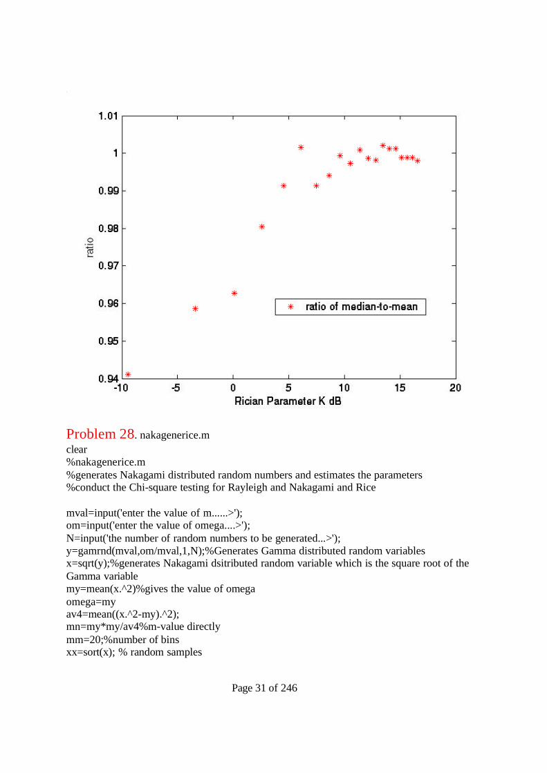
%computation of the outage probabilitiespower_ray=env_ray.^2;powerdB=10*log10(power_ray);mean_power=10*log10(mean(env_ray.^2))MK=length(env_ray)for k=1:20; pow(k)=mean_power-2*k; %threshold power kps=pow(k); ratio=10^(kps/10)/10^(mean_power/10); poutth(k)=1-exp(-ratio);%theoretical outage count=0; for ku=1:MK; power=powerdB(ku);%power in dB if power <= kps count=count+1; else end; end; poutsim(k)=count/MK;%outage probability simulatedend;figureplot(pow,poutth,':',pow,poutsim,'--'),title('Outage ---Rayleigh')xlabel('threshold power dBm')

of 246

ylabel('outage probability')legend('pout_{th}','pout_{sim}')

Problem 35. riceout1.m

clear%riceout1.m%generates a fading signal where a direct (LOS) component is present%generates the RF signal and calculate the outageclose allnumpaths = 10; %number of pathsFc = 900e6; %carrier frequencyFs = 4*Fc; %sampling frequencyTs = 1/Fs; %sampling periodt = [0:Ts:1999*Ts]; %time arraywc = 2*pi*Fc; %radian frequencyrice = zeros(1,length(t)); %received signalfor i = 1:numpaths-1

a = weibrnd(1,3,1,length(t)); %scattering strengtsh are Weibull distributed

of 246

rice = rice + a.*cos(wc*t+unifrnd(0,2*pi,1,length(t)));end;rice = rice + 4.5*cos(wc*t);%adds the direct path[ricei riceq] = demod(rice,Fc,Fs,'qam'); %demodulated signalenv_rice = sqrt(ricei.^2+riceq.^2); %envelope of received signalb = sqrt((std(ricei)^2 + std(riceq)^2)/2); %Rician parametera = mean(ricei); %Rician parameterpower_rice=env_rice.^2;powerdB=10*log10(power_rice);mean_power=10*log10(mean(env_rice.^2))MK=length(env_rice)for k=1:20; pow(k)=mean_power-2*k; %threshold power kps=pow(k); count=0; for ku=1:MK; power=powerdB(ku);%power in dB if power <= kps count=count+1; else end; end; poutsim(k)=count/MK;%outage probability simulated kbs=10^(kps/10);%power in mW poutth(k)=1-marcumq(a/b,sqrt(kbs)/b);%from the communications toolboxend;figureplot(pow,poutsim,pow,poutth),title('Outage ---Rician')xlabel('thrshold power dBm')ylabel('outage probability')legend('poutth','poutsim')

of 246

Problem 36.lognormf.m

clearclose all%exploration of the generation of lognormal%lognormf.m%generates a set of lognormal random numbers based on the principle that the procuct of a set ofrandom%numbers will give rise to lognormalmm=input('number of components for the product operation to check for lognormal..');for k=1:1000; x(k)=prod(raylrnd(1,1,mm));%generates the product of mm Rayleigh random numbersend;subplot(2,1,1)hist(x),title('histogram of the product of Rayleigh numbers')xlabel('volt')yy=10*log10(x.^2);subplot(2,1,2)hist(yy),title('histogram after conversion..10log_{10}x^2..')xlabel('dBm')

of 246

%Tests for Normal distribution m=20;%number of bins for the chi-square testy=sort(yy); % sort samplesN=length(y);mean=mean(y);stdev=std(y);inter=max(y)-min(y); %interval for chi-square testintstep=inter/m; %size of sub-intervalintval=[min(y):intstep:max(y)]; %samples at the sub-intervalsk=[zeros(1,m)]; %number of samples in each sub-interval intialization



np=p.*N;

q=0;for i=1:m q = q + ((k(i)-np(i))^2)/np(i); %chi-square testend;chi_square_val=q

of 246

Problem 37. fadlogfm.m

%fadlogfm.m%explores the generation of lognormal fading. There is multiple scattering. There are alsomultiple paths.%This will lead to Rayleigh envelope where the mean of the envelope will be randomclearclose all%simulates lognormal fadingfc=1e5;%carrier frequencyppf=2*pi*fc;N=11;% Number of mutiple paths%a are considered to be Gamma distributedfs=4*fc;%sampling rateTs=1/fs;t = [0:Ts:1999*Ts]; %time arraynn=length(t);

for kr=1:1000;%1000 rf waveforms are genaretd to see the statistics of the mean and the meadianpowers %multiple reflections

of 246

% %ggm is the result of multiple scattering; thus each multipath is produced by multiple(20)scattering. %the statistics of the mean and median of the Rayleigh have been computed. %NOTE THAT THE MULTIPLE REFLECTIONS OCCUR FIRST AND THEN THISMULTIPLY REFLECTED COMPONENTS %GET REFLECTED/SCATTERED/DIFFRACTED TO TAKE MULTIPLE PATHS TOTHE RECEIVER. %THE MULTIPLE SCATTERING COMPONENTS IDENTIFIED BY EACH OF THEggm %WILL BE RAYLEIGH DUE TO THE PRESENCE OF MUTIPLE SCATTERERS INTHE REGION %IN WHICH THE THE SCATTERING TAKES PLACE. ggm=prod(raylrnd(1.5,1,20));%generates the product of 20 Rayleigh r.v cr=zeros(1,nn); for m=1:N; phterm=2*pi*unifrnd(0,2*pi,1,nn); cr=cr+ggm*cos(ppf*t+phterm);%Rayleighend;[x,y]=demod(cr,fc,fs,'qam');ae=(1/N)*sqrt(x.^2+y.^2);%ae will be Rayleighae=ae;mm(kr)=mean(ae);med(kr)=median(ae);end;mm2=mm.^2;med2=med.^2;mmdB=10*log10(mm2);%mean power in dBmmeddB=10*log10(med2);%median power in dBm

%%% note that both average ( or median) of envelope and average of the power will belognormal

plot(t*1e3,cr/max(abs(cr))),title('rf signal incorporating lognormal fading');xlabel('time ms')ylabel('rf signal volt')xlim([0 0.5])

figuresubplot(2,2,1)hist(mm),title('histogram of the mean power')xlabel('volt')subplot(2,2,2)hist(med),title('histogram of the median power')xlabel('volt')

of 246

subplot(2,2,3)hist(mmdB),title('histogram of the mean power (dBm)')xlabel('dBm')subplot(2,2,4)hist(meddB),title('histogram of the median power (dBm)')xlabel('dBm')

Problem 38. fadlogfm.m (See the previous problem # 37)

of 246

Problem 39.lognormf.mclearclose all%exploration of the generation of lognormal%lognormf.m%generates a set of lognormal random numbers based on the principle that the procuct of a set ofrandom%numbers will give rise to lognormalmm=input('number of components for the product operation to check for lognormal..');for k=1:1000; x(k)=prod(raylrnd(1,1,mm));%generates the product of mm Rayleigh random numbersend;subplot(2,1,1)hist(x),title('histogram of the product of Rayleigh numbers')xlabel('volt')yy=10*log10(x.^2);subplot(2,1,2)hist(yy),title('histogram after conversion..10log_{10}x^2..')xlabel('dBm')

of 246

%Tests for Normal distribution m=20;%number of bins for the chi-square testy=sort(yy); % sort samplesN=length(y);mean=mean(y);stdev=std(y);inter=max(y)-min(y); %interval for chi-square testintstep=inter/m; %size of sub-intervalintval=[min(y):intstep:max(y)]; %samples at the sub-intervalsk=[zeros(1,m)]; %number of samples in each sub-interval intialization


Problem 40. lognormfchi.m

clearclose all%exploration of the generation of lognormal%lognormfchi.m%generates a set of lognormal random numbers based on the principle that the procuct of a set ofrandom%numbers will give rise to lognormal%chi-square tests directly and indirectly using Gaussianmm=input('number of components for the product operation to check for lognormal..');for k=1:1000; x(k)=prod(raylrnd(1,1,mm));%generates the product of mm Rayleigh random numbersend;subplot(2,1,1)hist(x),title('histogram of the product of Rayleigh numbers')xlabel('volt')yy=10*log10(x.^2);subplot(2,1,2)hist(yy),title('histogram after conversion..10log_{10}x^2..')xlabel('dBm')

%%% testing directly for lognormalm=20;

of 246

N=length(x);%Tests for lognormal distribution%[chu)]=chilogn(samp,bins)y=sort(x); % random samplesms=std(log(y));%sigma of the lognormal *** not the standard deviationinter=max(y)-min(y); %interval for chi-square testintstep=inter/m; %size of sub-intervalintval=[min(y):intstep:max(y)]; %samples at the sub-intervalsk=[zeros(1,m)]; %number of samples in each sub-interval intialization

for i=1:N for j=1:m if y(i)<=intval(j+1) k(j)=k(j)+1; break; end; end;end;my=mean(log(y));%parameter mu of the lognormal pdf*** not the mean of lognormalp=zeros(1,m);for i=1:m p(i)=logncdf(intval(i+1),my,ms)-logncdf(intval(i),my,ms); %probabilities at the sub-intervalsamplesend;

np=p.*N;

q=0;for i=1:m q = q + ((k(i)-np(i))^2)/np(i); %chi-square testend;ch_lognorm_val=q

clear qclear y%Tests for Normal distributionm=20;%number of bins for the chi-square testy=sort(yy); % sort samplesN=length(y);mean=mean(y);stdev=std(y);inter=max(y)-min(y); %interval for chi-square testintstep=inter/m; %size of sub-intervalintval=[min(y):intstep:max(y)]; %samples at the sub-intervalsk=[zeros(1,m)]; %number of samples in each sub-interval intialization

of 246



np=p.*N;

q=0;for i=1:m q = q + ((k(i)-np(i))^2)/np(i); %chi-square testend;chi_square_val=q

Problem 41.hatawalf.m

clearclose all% hatawalf.m Power loss calculations%using Hata model and Walfischcarf=880;%carrier frequency of in MHzlcrf=log10(carf);ht=30;%height in meters of the BSlht=log10(ht);hr=1.5;%MU ant. height in meterslhr=log10(11.75*hr);N=60;%number of increments for distancedistmax=30;%coverage distance in Kmsfor kk=1:30;d(kk)=1+0.5*(kk-1);fact1=69.55+26.16*lcrf-13.83*lht;fact2=(44.9-6.55*lht)*log10(d(kk));fftq=fact1+fact2;%antenna correction factor MU...ahr=3.2*(lhr)^2-4.97;% large cities; freq. above 400 MHz

of 246

amr=(1.1*lcrf-0.7)*hr-(1.56*lcrf-0.8);alar(kk)=fftq-ahr;%Hata model

lfree=32.4+20*log10(d(kk))+20*lcrf;%free space losssw=15;%street widthhb=30;%building height=antenna height=separation of buildingsdhb=0;%no difference in heights of bdg and antennadhm=hb-hr;ang=90;%angle philrts=-16.9+10*lcrf-10*log10(sw)+20*log10(dhm)+4-.114*90;lms=0+54+18*log10(d(kk))+(-4+1.5*(carf/925-1))*lcrf-9*log10(hb);alf(kk)=lfree+lrts+lms;%W-I modelend;

plot(d,alar,d,alf); legend('Hata model','Walfish-Ikegami model') %axis([1 30 -140 -60]); xlabel('distance Km'); ylabel('power loss dB'); %for transfering to excel directly as columns d=d'; alf=alf'; alar=alar';

of 246

Problem 42. See the textbook; relevant sections

Problem 43. See the textbook; relevant sections

Problem 44. coheBW.m

%coheBW.m%plot of the correlation of faded channelsclearclose allfor k=1:50; x(k)=0.05*(k-1); x1=x(k); sigma=1; y(k)=1/(1+(2*pi*x1*sigma)^2);%corr coef. freq y1=besselj(0,2*pi*x1); yy(k)=y1^2;%corr. Coeff timeend;

of 246

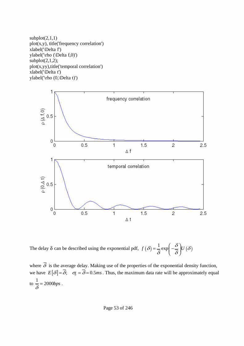
subplot(2,1,1)plot(x,y), title('frequency correlation')xlabel('\Delta f')ylabel('\rho (\Delta f,0)')subplot(2,1,2);plot(x,yy),title('temporal correlation')xlabel('\Delta t')ylabel('\rho (0,\Delta t)')

The delay can be described using the exponential pdf, 1 expf U

where is the average delay. Making use of the properties of the exponential density function,we have ; 0.5E ms . Thus, the maximum data rate will be approximately equal

to 1

2000bps

.

of 246

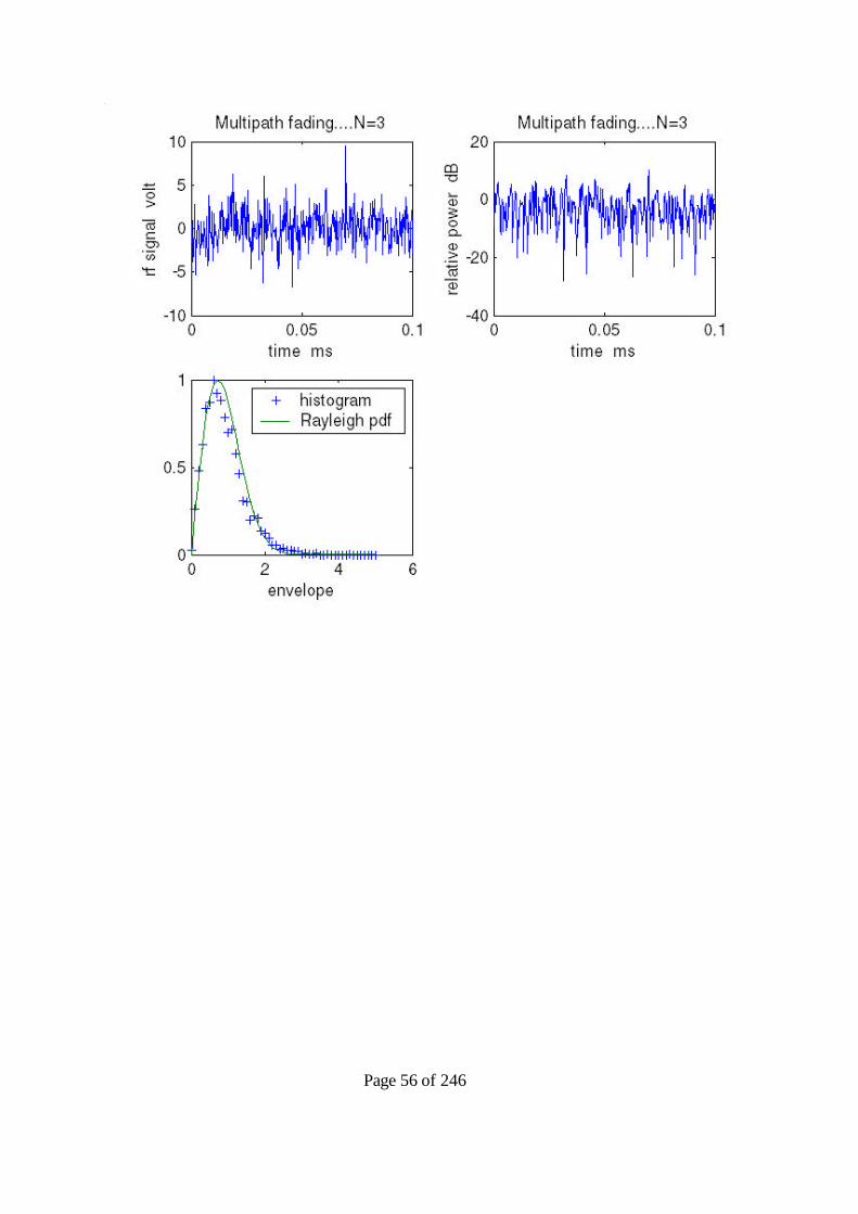
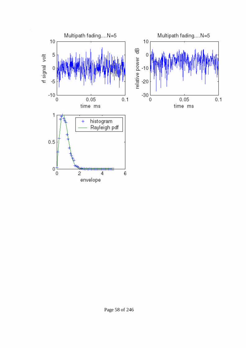
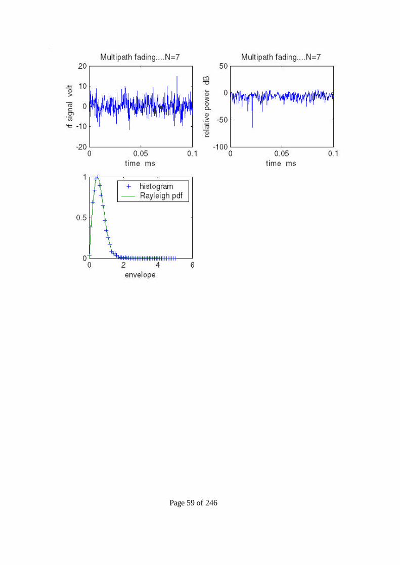
Problem 45.fadcomRayl. m and chirayleigh.m (see next problem)

clear%fadcomRayl.m simulates multiptah fading varying the number of paths%Compares the histogram to a Rayleigh pdfclose allfc=900e3;%carrier frequencyppf=2*pi*fc;N1=[3 5 7 10]%a are considered to be Gamma distributedfs=4*fc;%sampling ratedt=1/fs;nn=1e-3/dt;%total number of samples in one m secM=2^(nextpow2(nn))dist=1000;%distance between transmit and receive in metersavdel=dist/3e8;%average delay in secondsfor kmm=1:4 N=N1(kmm)for k=1:nn; t(k)=k*dt; ci=0.0; cir=0.0; for m=1:N; phterm=2*pi*rand(1); ci=ci+gamrnd(1.4,1)*cos(ppf*t(k)+phterm);%Rayleigh including Dopplerend;cr(k)=ci;end;[x,y]=demod(cr,fc,fs,'qam');ae=(1/N)*sqrt(x.^2+y.^2); pha=pi+angle(x+i*y);%phase to be centered around 2*pi numb=num2str(N); fx=strcat('Multipath fading....','N=',numb); figuresubplot(2,2,1)plot(t*1e3,cr),title(fx)xlabel('time ms')ylabel('rf signal volt')xlim([0 .1])aes=20*log10(ae);subplot(2,2,2)plot(t*1e3,aes),title(fx)xlabel('time ms')ylabel('relative power dB')xlim([0 .1])

of 246

subplot(2,2,3)ax=0.:0.1:5;% range of values for the histogramyy=hist(ae,ax);bb=mean(ae)*sqrt(2/pi);%Rayleigh parameter by=raylpdf(ax,bb);%Rayl density function of parameter bplot(ax,yy/max(yy),'+',ax,y/max(y)),title(fx)legend('histogram','Rayleigh pdf')xlabel('envelope')qq=chirayleigh(ae,20)%chi-square valueend;

of 246

of 246

Problem 46.fadconRayl (see previous problem) and chirayleigh

function [q]=chirayleigh(yy,m)%Tests for Rayleigh distribution%[chu)]=chirayleigh(samp,bins)y=sort(yy); % random samplesN=length(yy);my=mean(yy);%meaninter=max(y)-min(y); %interval for chi-square testintstep=inter/m; %size of sub-intervalintval=[min(y):intstep:max(y)]; %samples at the sub-intervalsk=[zeros(1,m)]; %number of samples in each sub-interval intialization

for i=1:N for j=1:m if y(i)<=intval(j+1) k(j)=k(j)+1; break; end;

of 246

end;end;

myp=my*sqrt(2/pi);%Rayleigh parameterp=zeros(1,m);for i=1:m p(i)=raylcdf(intval(i+1),myp)-raylcdf(intval(i),myp); %probabilities at the sub-interval samplesend;

np=p.*N;


N = 3; Chi-square value = 4.7997e+003

N = 5; Chi-square value = 380.6133



Problem 47 .pulsefading.m

clear%pulsefading.m fading including a carrier frequency%three delays are created; Pulse stream is delayed and added%the a uniform phase is introduced in the RF pulse stream; three pulses are addedclose all%examines the fading of pulse/shapes%the program prompts the fractional delays

fc=10e3;%carrier frequencyppf=2*pi*fc;fs=12*fc;%sampling rateddt=1/fs;nn=1e-3/ddt;%total number of samples in one m secM=2^(nextpow2(nn))dist=1000;%distance between transmit and receive in meters

of 246

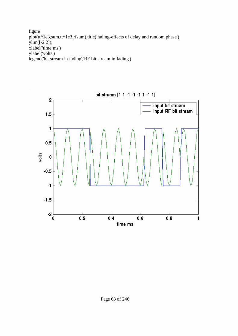
avdel=dist/3e8;%average delay in seconds%kp*ku:kp*ku+1N=8;%number of bitsa=[1 1 -1 -1 -1 1 -1 1];kp=floor(nn/8);%creates the width of the pulsefor ku=1:8;for k=(ku-1)*kp+1:kp*ku tt(k)=k*ddt; s(k)=a(ku);%creates the pulse stream sf(k)=a(ku)*cos(ppf*tt(k));%rf pulse sf1(k)=a(ku)*cos(ppf*tt(k)+2*pi*rand(1));%random phase sf2(k)=a(ku)*cos(ppf*tt(k)+2*pi*rand(1));%random phase end;end;

del=input('enter the fractional (of the duration) delay...between 0.25 and 0.75..');dd1=round(del*kp);for k=1:kp*ku; if k<=dd1 ss1(k)=0;else ss1(k)=s(k-dd1);%creates a delayed pulse streamend;end;del2=input('enter the fractional (of the duration) delay...between 0.25 and 0.75..');dd2=round(del2*kp);for k=1:kp*ku; tt2(k)=k*ddt; if k<=dd2 ss2(k)=0;else ss2(k)=s(k-dd2);%creates a delayed pulseend;end;sum=s+ss1+ss2;%added pulse shapessum=sum/max(abs(sum));%normalizes to unityrfsum=sf+sf1+sf2;%added RF pulsesrfsum=rfsum/max(abs(rfsum));%normalizes to unity

plot(tt*1e3,s,tt*1e3,sf),title('bit stream [1 1 -1 -1 -1 1 -1 1]')ylim([-2 2]);xlabel('time ms')ylabel('volts')legend('input bit stream','input RF bit stream')

of 246

figureplot(tt*1e3,sum,tt*1e3,rfsum),title('fading-effects of delay and random phase')ylim([-2 2]);xlabel('time ms')ylabel('volts')legend('bit stream in fading','RF bit stream in fading')

of 246

Problem 48. pulsefading

See the m file and results of the previous exercise (# 48)

Problem 49. pulsefadingRayl

clear%pulsefadingRayl.m fading including a carrier frequency%three delays are created; Pulse stream is delayed and added%three pulses are added%includes Rayleigh weighting at each time instant%the program prompts the fractional delaysclose all%examines the fading of pulse/shapesfc=10e3;%carrier frequencyppf=2*pi*fc;fs=12*fc;%sampling rateddt=1/fs;

of 246

nn=1e-3/ddt;%total number of samples in one m secM=2^(nextpow2(nn))dist=1000;%distance between transmit and receive in metersavdel=dist/3e8;%average delay in seconds%kp*ku:kp*ku+1N=8;%number of bitsa=[1 1 -1 -1 -1 1 -1 1];kp=floor(nn/8);%creates the width of the pulsefor ku=1:8;for k=(ku-1)*kp+1:kp*ku tt(k)=k*ddt; s(k)=a(ku);%creates the pulse stream ss1(k)=a(ku)*raylrnd(1);%Rayleigh weighted sf(k)=a(ku)*cos(ppf*tt(k));%rf pulse sf1(k)=raylrnd(1)*a(ku)*cos(ppf*tt(k));%rf pulse Rayleigh weighted sf2(k)=raylrnd(1)*a(ku)*cos(ppf*tt(k));%rf pulse Rayleigh weighted sf3(k)=raylrnd(1)*a(ku)*cos(ppf*tt(k));%rf pulse Rayleigh weighted end;end;

del=input('enter the fractional (of the duration) delay...between 0.25 and 0.75..');dd1=round(del*kp);for k=1:kp*ku; if k<=dd1 ss2(k)=0;else ss2(k)=s(k-dd1)*raylrnd(1);end;end;del2=input('enter the fractional (of the duration) delay...between 0.25 and 0.75..');dd2=round(del2*kp);for k=1:kp*ku;

if k<=dd2 ss3(k)=0;else ss3(k)=s(k-dd2)*raylrnd(1);end;end;sum=ss1+ss2+ss3;%added pulse shapes;Rayleigh weightedsum=sum/max(abs(sum));%normalizes to unityrfsum=sf1+sf2+sf3;%added RF pulses Rayleigh weightedrfsum=rfsum/max(abs(rfsum));%normalizes to unity

plot(tt*1e3,s,tt*1e3,sf),title('bit stream [1 1 -1 -1 -1 1 -1 1]')ylim([-2 2]);

of 246

xlabel('time ms')ylabel('volts')legend('input bit stream','input RF bit stream')figureplot(tt*1e3,sum,tt*1e3,rfsum),title('Rayleigh weighted fading')ylim([-2 2]);xlabel('time ms')ylabel('volts')legend('bit stream in fading','RF bit stream in fading')

of 246

Problem 50. pulsefadingRayl

See exercise # 49.

bai giai truyen thong khong day moi

Documents