bad decisions - editorial express
TRANSCRIPT

GoBack

John Rust Bad Decisions - slide #1
Bad Decisions
John RustUniversity of Maryland


● Bad Decisions
The Singularity is Near
● A book by Ray Kurzweil
(Viking Press, 2005)
● The Six Epochs
● The New Growth Theory –
Loglog scaling
● The Accelerating Rate of
Change
● The New Growth Theory –
Semilog scaling
● What to make of these
predictions?● Humans now control evolution
● The Value of Models
John Rust Bad Decisions - slide #3
A book by Ray Kurzweil (Viking Press, 2005)
1. The singularity is not armageddon nor a dire prediction ofNostradamus!
2. But it does fortell an inevitable cataclysmic change in theworld.
3. “I set the date for the Singularity — representing a profoundand disruptive transformation in human capability — as2045. The nonbiological intelligence created in that year willbe one billion times more powerful than human intelligencetoday.” Kurzweil, p. 136
4. Changes in technology and human evolution will soprofound and so rapid that it is impossible to predict what lifewill like after the singularity — it is beyond our “eventhorizon”.
5. In particular humanity, as we now know it will be obsolete —superseded by a new generation of super intelligent quasibiological androids — andro super sapiens.

John Rust Bad Decisions - slide #4
The Six Epochs
Information in atomic structures
Information in DNA
Information in neural patterns
Information in hardware and software designs
The methods of biology (including human intelligence) are
integrated into the (exponentially expanding) human technology base
Patterns of matter and energy in the universe become
saturated with intelligent processes and knowledge
Epoch 1 Physics and Chemistry
Epoch 2 Biology
Epoch 3 Brains
Epoch 4 Technology
Epoch 5 Merger of Technology
and Human Intelligence
Epoch 6 The Universe Wakes Up
DNA evolves
Brains evolve
Technology evolves
Technology masters the
methods of biology
(including human intelligence)
Vastly expanded human
intelligence (predominantly
nonbiological) spreads
through the universe
The Six Epochs of EvolutionEvolution works through indirection: it creates
a capability and then uses that capability to
evolve the next stage.
John Rust Bad Decisions - slide #5
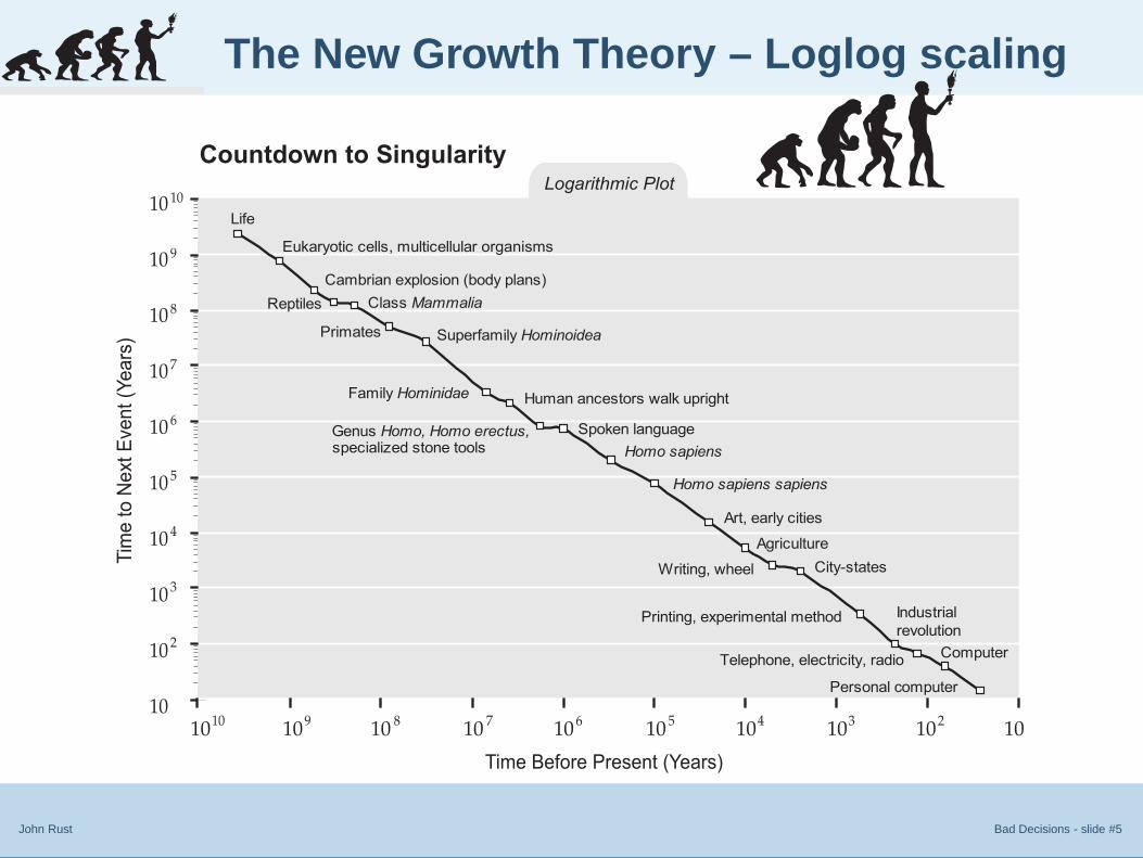
The New Growth Theory – Loglog scaling
Countdown to Singularity: Biological evolution and human technology
Time Before Present (Years)
Tim
e to N
ext E
vent (Y
ears
)
10 10 10 10 10 10 10 10 10 10
10
9
8
7
6
5
4
3
2
10
10
10
10
10
10
10
10
10
1010 9 8 7 6 5 4 3 2
Eukaryotic cells, multicellular organisms
Personal computer
ComputerTelephone, electricity, radio
Printing, experimental method Industrial
revolution
City-statesWriting, wheel
Agriculture
Art, early cities
Homo sapiens sapiens
Homo sapiens
Spoken languageGenus Homo, Homo erectus, specialized stone tools
Human ancestors walk uprightFamily Hominidae
Superfamily HominoideaPrimates
Class MammaliaReptiles
Cambrian explosion (body plans)
Life
Countdown to SingularityLogarithmic Plot

● Bad Decisions
The Singularity is Near
● A book by Ray Kurzweil
(Viking Press, 2005)
● The Six Epochs
● The New Growth Theory –
Loglog scaling
● The Accelerating Rate of
Change
● The New Growth Theory –
Semilog scaling
● What to make of these
predictions?● Humans now control evolution
● The Value of Models
John Rust Bad Decisions - slide #6
The Accelerating Rate of Change
■ “Two billion years ago our ancestors were microbes; ahalf-billion years ago, fish; a hundred million years ago,something like mice, ten million years ago, arboreal apes;and a million years ago, proto-humans puzzling out thetaming of fire.
■ Our evolutionary lineage is marked by the mastery ofchange. In our time, thepace is quickening.
■ Carl Sagan

John Rust Bad Decisions - slide #7
The New Growth Theory – Semilog scaling
Linear Plot
Time Before Present (Years)
Tim
e to N
ext E
vent (Y
ears
)
10
9
8
7
6
5
4
3
2
10
10
10
10
10
10
10
10
10
10
Life
Cambrian explosion (body plans)Reptiles
Class Mammalia
PrimatesSuperfamily Hominoidea
Family Hominidae
Human ancestors walk upright
Genus Homo, Homo erectus,specialized stone tools
Homo sapiens
Homo sapiens sapiens
Art, early cities
Agriculture
Writing, wheelCity-states
Industrial revolution
Printing, experimental method
Telephone, electricity, radioComputer
Personal computer
Eukaryotic cells,
multicellular organisms
0102x103x104x109 9 9 9
Countdown to Singularity
● Bad Decisions
The Singularity is Near
● A book by Ray Kurzweil
(Viking Press, 2005)
● The Six Epochs
● The New Growth Theory –
Loglog scaling
● The Accelerating Rate of
Change
● The New Growth Theory –
Semilog scaling
● What to make of these
predictions?● Humans now control evolution
● The Value of Models
John Rust Bad Decisions - slide #8
What to make of these predictions?
1. To some extent, they seem too optimistic
● Bad Decisions
The Singularity is Near
● A book by Ray Kurzweil
(Viking Press, 2005)
● The Six Epochs
● The New Growth Theory –
Loglog scaling
● The Accelerating Rate of
Change
● The New Growth Theory –
Semilog scaling
● What to make of these
predictions?● Humans now control evolution
● The Value of Models
John Rust Bad Decisions - slide #8
What to make of these predictions?
1. To some extent, they seem too optimistic2. Recall Ray Clark/Stanley Kubrick’s predictions of the power
of the computer Hal, in 2001: A Space Odessy
3. The movie came out in 1969, and in it, Hal came online inUrbana, Illinois in 1998.
4. Although the Cray 2 supercomputer was operating inUrbana in 1998, its powers and abilities were far short ofHal’s.
5. However we cannot deny Moore’s Law. It corresponds to anexponential growth rate of 46% per year!
6. In 1997 the peak speed of the Cray 2 was 1.9 gigaflops. In2007 IBM’s new Blue Gene/P supercomputer will perform inthe petaflops — one million times faster than the Cray 2!
7. 1997 is also significant: it marks the year when IBM’s DeepBlue defeated Garry Kasparov. Ever since then the world’sbest chess players have been computers!

● Bad Decisions
The Singularity is Near
● A book by Ray Kurzweil
(Viking Press, 2005)
● The Six Epochs
● The New Growth Theory –
Loglog scaling
● The Accelerating Rate of
Change
● The New Growth Theory –
Semilog scaling
● What to make of these
predictions?● Humans now control evolution
● The Value of Models
John Rust Bad Decisions - slide #9
Humans now control evolution
1. Eckard Wimmer created the first artificial virus in 2002. Wecan clone sheep, build artificial organs, and in less than adecade humans will be creating artificial life.
2. A June 2006 Scientific American article by the “bio fabgroup” describes “Engineering LIfe: Building a Fab forBiology” “We are progressing toward first designing andmodeling biological devices in computer, then ‘cutting’ theminto biological form as the final step — much as silicon chipsare planned, then etched.” (p. 51)
3. The result is a huge speedup in the rate of evolution: “Thesetechnologies — releasable parallel synthesis and errorcorrection — permit us to assemble long, relativelyerror-free DNA constructs far more rapidly andinexpensively than has been possible to date. They cantherefore constitute basis of a bio fab, and much likesemiconductor chip lithography, these processes can beexpected to keep steadily improving over time. That frees usto think about what we will build in the fab. (p. 48).

● Bad Decisions
The Singularity is Near
● A book by Ray Kurzweil
(Viking Press, 2005)
● The Six Epochs
● The New Growth Theory –
Loglog scaling
● The Accelerating Rate of
Change
● The New Growth Theory –
Semilog scaling
● What to make of these
predictions?● Humans now control evolution
● The Value of Models
John Rust Bad Decisions - slide #10
The Value of Models
■ “Our ability to create models — virtual realities — in ourbrains, combined with our modest looking thumbs, has beensufficient to usher in another form of evolution: technology.That development enabled the persistence of theaccelerating pace that started with biological evolution. It willcontinue until the entire universe is at our fingertips.”
■ Ray Kurzweil, p. 487, concluding sentences of TheSingularity is Near

GoBack

John Rust Bad Decisions - slide #1
Bad Decisions
John RustUniversity of Maryland

John Rust Bad Decisions - slide #2
If we are so smart, why are we so dumb?

● Bad Decisions
If we are so smart why are we
so dumb?
● The state of the world in
2006? Terrible!● Many of our leaders make
bad decisions● Floyd Landis
● Bill Clinton
● Kim Jong-Il
● Kenny Lay
● Saddam Hussein
● Saddam in Happier Times
● Tony Blair
● “Observing” Ex Ante Beliefs
John Rust Bad Decisions - slide #3
The state of the world in 2006? Terrible!1. If technology is transporting us to the “promised land”, we
seem at the very least to be taking a very big detour lately.

● Bad Decisions
If we are so smart why are we
so dumb?
● The state of the world in
2006? Terrible!● Many of our leaders make
bad decisions● Floyd Landis
● Bill Clinton
● Kim Jong-Il
● Kenny Lay
● Saddam Hussein
● Saddam in Happier Times
● Tony Blair
● “Observing” Ex Ante Beliefs
John Rust Bad Decisions - slide #3
The state of the world in 2006? Terrible!1. If technology is transporting us to the “promised land”, we
seem at the very least to be taking a very big detour lately.2. Corruption, bigotry, hatred, terrorism, religious fanaticism,
civil war, genocide, threat of nuclear war, and increasingignorance, indifference, and inequality: the world doesnothing as preventable genocide occurs in places such asRwanda and Darfur. Many parts of the world (e.g.India/Pakistan, Middle East) are dangerously unstable.Some pundits now say we are on the verge of World War III.
3. Technology has both good and bad uses. Human progressis slowed because for every positive technologicaldevelopment, we find a way to use it as a weapon to injure,destroy, and kill each other.
4. Our increasingly sophisticated technologies are still affectedby neanderthal instincts in our primitive mamallian brains,including primitive urges to rape, plunder, pillage, and kill.Our ability to make rational decisions is compromised byhormones such as testosterone, cortisone, adrenaline, andother sex and “flight or fight” hormones.

● Bad Decisions
If we are so smart why are we
so dumb?
● The state of the world in
2006? Terrible!● Many of our leaders make
bad decisions● Floyd Landis
● Bill Clinton
● Kim Jong-Il
● Kenny Lay
● Saddam Hussein
● Saddam in Happier Times
● Tony Blair
● “Observing” Ex Ante Beliefs
John Rust Bad Decisions - slide #4
Many of our leaders make bad decisions1. I blame many of the world’s problems on bad decisions by
our leaders, some of whom are consistently bad decisionmakers.
2. The processes we use to choose the leaders of our nationsand corporations are highly imperfect, and even deeplycorrupt (and in the US and many other countriesincreasingly corrupt).
3. As a result, bad leaders frequently come to power, and evengood leaders can occasionally make very bad decisionswith far reaching consequences. The “checks and balances”available for curtailing the power of bad decision makers areoften limited or ineffective.
4. Bad decision making can be history-dependent: it cancreate social level collective “illnesses” and hatreds that canprogate for generations. Examples: Nazism, and manykinds of reglious extremism (e.g. the Crusades).
5. I now present several examples of bad decisions and baddecision makers. Then I will define what I mean by “baddecision.”


John Rust Bad Decisions - slide #6
Bill Clinton
Click here to see Bill perform


John Rust Bad Decisions - slide #10
Saddam in Happier Times
(shown after receiving billions in U.S. arms from Donald Rumsfeld)


● Bad Decisions
If we are so smart why are we
so dumb?
● The state of the world in
2006? Terrible!● Many of our leaders make
bad decisions● Floyd Landis
● Bill Clinton
● Kim Jong-Il
● Kenny Lay
● Saddam Hussein
● Saddam in Happier Times
● Tony Blair
● “Observing” Ex Ante Beliefs
John Rust Bad Decisions - slide #12
“Observing” Ex Ante Beliefs1. The “Downing Street memos” give insights into the
subjective beliefs held by Blair prior to the Iraq war. JackStraw memo to Tony Blair, March 25, 2002, preparing Blairfor meeting at Bush’s ranch in Crawford, Texas.
2. “The rewards to your visit to Crawford will be few. The riskswill be high both for you and the Government. . . . But wehave a long way to go as to: a) the scale of the threat fromIraq and why this has got worse recently, b) whatdistinguishes the threat from that eg of Iran and North Koreaso as to justify military action;”
3. “We have to answer the big question — what will this actionachieve? There seems to be a larger hole in this than onanything.”
4. “Most of the assessments from the US have assumedregime change as a means of eliminating Iraq’s WMDthreat. But none has satisfactorily answered how thatregime change is to be secured, and how there can be anycertainty that the replacement regime will be any better.”

John Rust Bad Decisions - slide #13
Last but not least, the “king” of bad decisionmakers


John Rust Bad Decisions - slide #15
Who makes the decisions: Bush or Cheney?

John Rust Bad Decisions - slide #17
The 2006 “Bush Prize” for Bad Decision Making

John Rust Bad Decisions - slide #18
2006 Bush Prize for Bad Decision Making
A Joint Award to Hassan Nasrullan and Ehud Olmert

● Bad Decisions
2006 Prize for Bad Decision
Making
● 2006 Bush Prize for Bad
Decision Making
● How to define a “bad
decision”?● Definition of a bad decision
● Definition of a bad decision,
continued● Definition of a crazy decision
● Comments on the concept
● Problems with the concept
● The Identification Problem
● Subjective beliefs are
endogenous
● The Role of Expert advisors
● A Bush war advisor, now a
Bush war critic● Biased advice and the Iraq
war decision● Scientific advice and good
decisions● Scientific Advice and George
Bush● The Problem of “20-20
Hindsight”
John Rust Bad Decisions - slide #19
How to define a “bad decision”?
1. I wish to avoid a typical blunder, which is to judge ex antedecisions in terms of the “20-20 hindsight” of having seen expost outcomes.
2. I wish to separate the question of morality of a bad decisionand focus on the rationality of the decision maker.
3. Thus, I wish to abstract from issues of “right” and “wrong”even though in common parlance, bad decision arefrequently viewed as ones that are immoral or illegal.
4. Questions of morality are more in the domain of religion,philosophy, and politics. I am an economist.
5. Instead, I adopt a common approach in economics,consumer sovereignty, and do not question the decisionmaker’s utility function.
6. The common feature of all the examples I presented aredecision makers with seriously distorted perceptions ofreality.
● Bad Decisions
2006 Prize for Bad Decision
Making
● 2006 Bush Prize for Bad
Decision Making
● How to define a “bad
decision”?● Definition of a bad decision
● Definition of a bad decision,
continued● Definition of a crazy decision
● Comments on the concept
● Problems with the concept
● The Identification Problem
● Subjective beliefs are
endogenous
● The Role of Expert advisors
● A Bush war advisor, now a
Bush war critic● Biased advice and the Iraq
war decision● Scientific advice and good
decisions● Scientific Advice and George
Bush● The Problem of “20-20
Hindsight”
John Rust Bad Decisions - slide #20
Definition of a bad decision
1. Definition: A bad decision is a decision under uncertaintythat is made by a decision maker (DM) (according to eitheran expected utility or non-expected utility criterion) whosesubjective probability distribution that is greatly at oddsrelative to the objective probability distribution governing theex post payoff relevant states of nature in the sense that theloss (under the objective probability measure) from takingthe decision is large.
2. Consider the expected utility case. Let µs be the DM’ssubjective probability measure. Then the decision (anddecision rule) are defined by
δs(I) = argmax
d∈D(I)
Eµs{U(X, d)|I} ≡
∫x
U(x, d)µs(x|I)
● Bad Decisions
2006 Prize for Bad Decision
Making
● 2006 Bush Prize for Bad
Decision Making
● How to define a “bad
decision”?● Definition of a bad decision
● Definition of a bad decision,
continued● Definition of a crazy decision
● Comments on the concept
● Problems with the concept
● The Identification Problem
● Subjective beliefs are
endogenous
● The Role of Expert advisors
● A Bush war advisor, now a
Bush war critic● Biased advice and the Iraq
war decision● Scientific advice and good
decisions● Scientific Advice and George
Bush● The Problem of “20-20
Hindsight”
John Rust Bad Decisions - slide #20
Definition of a bad decision
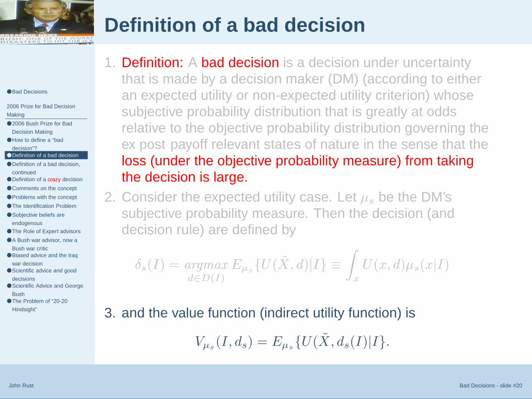
1. Definition: A bad decision is a decision under uncertaintythat is made by a decision maker (DM) (according to eitheran expected utility or non-expected utility criterion) whosesubjective probability distribution that is greatly at oddsrelative to the objective probability distribution governing theex post payoff relevant states of nature in the sense that theloss (under the objective probability measure) from takingthe decision is large.
2. Consider the expected utility case. Let µs be the DM’ssubjective probability measure. Then the decision (anddecision rule) are defined by
δs(I) = argmax
d∈D(I)
Eµs{U(X, d)|I} ≡
∫x
U(x, d)µs(x|I)
3. and the value function (indirect utility function) is
Vµs(I, ds) = Eµs
{U(X, ds(I)|I}.

● Bad Decisions
2006 Prize for Bad Decision
Making
● 2006 Bush Prize for Bad
Decision Making
● How to define a “bad
decision”?● Definition of a bad decision
● Definition of a bad decision,
continued● Definition of a crazy decision
● Comments on the concept
● Problems with the concept
● The Identification Problem
● Subjective beliefs are
endogenous
● The Role of Expert advisors
● A Bush war advisor, now a
Bush war critic● Biased advice and the Iraq
war decision● Scientific advice and good
decisions● Scientific Advice and George
Bush● The Problem of “20-20
Hindsight”
John Rust Bad Decisions - slide #21
Definition of a bad decision, continued
1. Let µo denote the objective probability measure and do thecorresponding optimal decision rule. Then we have
Vµs(I, ds) ≥ Vµs
(I, do).
2. I say d = ds(I) is a bad decision if
Vµo(I, do) − Vµo
(I, ds) > K > 0,
● Bad Decisions
2006 Prize for Bad Decision
Making
● 2006 Bush Prize for Bad
Decision Making
● How to define a “bad
decision”?● Definition of a bad decision
● Definition of a bad decision,
continued● Definition of a crazy decision
● Comments on the concept
● Problems with the concept
● The Identification Problem
● Subjective beliefs are
endogenous
● The Role of Expert advisors
● A Bush war advisor, now a
Bush war critic● Biased advice and the Iraq
war decision● Scientific advice and good
decisions● Scientific Advice and George
Bush● The Problem of “20-20
Hindsight”
John Rust Bad Decisions - slide #21
Definition of a bad decision, continued
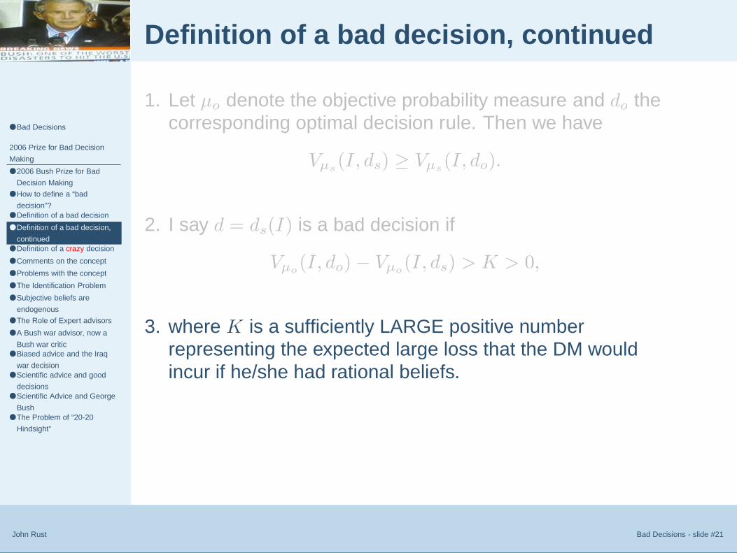
1. Let µo denote the objective probability measure and do thecorresponding optimal decision rule. Then we have
Vµs(I, ds) ≥ Vµs
(I, do).
2. I say d = ds(I) is a bad decision if
Vµo(I, do) − Vµo
(I, ds) > K > 0,
3. where K is a sufficiently LARGE positive numberrepresenting the expected large loss that the DM wouldincur if he/she had rational beliefs.

● Bad Decisions
2006 Prize for Bad Decision
Making
● 2006 Bush Prize for Bad
Decision Making
● How to define a “bad
decision”?● Definition of a bad decision
● Definition of a bad decision,
continued● Definition of a crazy decision
● Comments on the concept
● Problems with the concept
● The Identification Problem
● Subjective beliefs are
endogenous
● The Role of Expert advisors
● A Bush war advisor, now a
Bush war critic● Biased advice and the Iraq
war decision● Scientific advice and good
decisions● Scientific Advice and George
Bush● The Problem of “20-20
Hindsight”
John Rust Bad Decisions - slide #21
Definition of a bad decision, continued
1. Let µo denote the objective probability measure and do thecorresponding optimal decision rule. Then we have
Vµs(I, ds) ≥ Vµs
(I, do).
2. I say d = ds(I) is a bad decision if
Vµo(I, do) − Vµo
(I, ds) > K > 0,
3. where K is a sufficiently LARGE positive numberrepresenting the expected large loss that the DM wouldincur if he/she had rational beliefs.
4. In other words, if the DM had rational (or approximatelyrational) beliefs, he/she would never voluntarily choose tomake the bad decision.

● Bad Decisions
2006 Prize for Bad Decision
Making
● 2006 Bush Prize for Bad
Decision Making
● How to define a “bad
decision”?● Definition of a bad decision
● Definition of a bad decision,
continued● Definition of a crazy decision
● Comments on the concept
● Problems with the concept
● The Identification Problem
● Subjective beliefs are
endogenous
● The Role of Expert advisors
● A Bush war advisor, now a
Bush war critic● Biased advice and the Iraq
war decision● Scientific advice and good
decisions● Scientific Advice and George
Bush● The Problem of “20-20
Hindsight”
John Rust Bad Decisions - slide #22
Definition of a crazy decision1. Definition: A crazy decision is one that is taken even after a
credible authority has informed the DM that his/her beliefsare greatly at odds with the objective probability distributionand will result in very large ex ante losses. Further, the DMknows the decision will result in a high probability of verybad ex post losses, even relative to the DM’s distortedsubjective beliefs, but the DM does it anyway.
2. That is, a crazy decision is one that the DM refuses tochange, even after learning that their view of the world isgrossly incorrect and that their decision will result in large exante losses and a high probability of catastrophic ex postlosses.
3. Example: A daughter of “Christian scientists” has atreatable cancer but will surely die if chemotheory is notgiven immediately. The church tells the parents that it isconsistent with God’s will to give their daughterchemotherapy. The parents still refuse, flee with theirdaughter to avoid arrest, and she soon dies of cancer.
● Bad Decisions
2006 Prize for Bad Decision
Making
● 2006 Bush Prize for Bad
Decision Making
● How to define a “bad
decision”?● Definition of a bad decision
● Definition of a bad decision,
continued● Definition of a crazy decision
● Comments on the concept
● Problems with the concept
● The Identification Problem
● Subjective beliefs are
endogenous
● The Role of Expert advisors
● A Bush war advisor, now a
Bush war critic● Biased advice and the Iraq
war decision● Scientific advice and good
decisions● Scientific Advice and George
Bush● The Problem of “20-20
Hindsight”
John Rust Bad Decisions - slide #23
Comments on the concept
1. Note that bad decisions and crazy decisions could be onesthat are overly cautious due to excessive pessimism orexaggerated subjective riskiness,
2. or they could be ones that involve excessive risk taking dueto excessive optimism or underestimated subjectiveriskiness.
3. Bad decisions can have good ex post outcomes, just asgood decisions can have bad ex post outcomes.
4. However the focus should be on the quality of the ex antedecision making, and the care, and level of effort thedecision maker devotes to learn the objective probabilitydistribution governing ex post outcomes.
5. “Unfortunately, Washington — the political process and themedia — judges decisions based solely on outcomes, noton the quality of the decision making.” Robert Rubin, from2003 memoire, In an Uncertain World
● Bad Decisions
2006 Prize for Bad Decision
Making
● 2006 Bush Prize for Bad
Decision Making
● How to define a “bad
decision”?● Definition of a bad decision
● Definition of a bad decision,
continued● Definition of a crazy decision
● Comments on the concept
● Problems with the concept
● The Identification Problem
● Subjective beliefs are
endogenous
● The Role of Expert advisors
● A Bush war advisor, now a
Bush war critic● Biased advice and the Iraq
war decision● Scientific advice and good
decisions● Scientific Advice and George
Bush● The Problem of “20-20
Hindsight”
John Rust Bad Decisions - slide #24
Problems with the concept
1. How can we identify a bad decision if nobody knows whatthe objective probability measure µo is?
2. This seems to be the case for any real world decision. If so,how can there be a strong, objective scientific basis forclassifying decisions as bad ones?
3. There is a real risk that any theory of subjective decisionswould devolve into a petty, political, and subjective sort ofdisagreement, of the form “my beliefs are more realistic thanyour beliefs.”
4. If I am unwilling to question preferences, and if I concedethat beliefs about most uncertain events in the real worldare unavoidably subjective, then on what grounds can Ijustify questioning another person’s beliefs?

● Bad Decisions
2006 Prize for Bad Decision
Making
● 2006 Bush Prize for Bad
Decision Making
● How to define a “bad
decision”?● Definition of a bad decision
● Definition of a bad decision,
continued● Definition of a crazy decision
● Comments on the concept
● Problems with the concept
● The Identification Problem
● Subjective beliefs are
endogenous
● The Role of Expert advisors
● A Bush war advisor, now a
Bush war critic● Biased advice and the Iraq
war decision● Scientific advice and good
decisions● Scientific Advice and George
Bush● The Problem of “20-20
Hindsight”
John Rust Bad Decisions - slide #25
The Identification Problem
1. Rust (1994) and Magnac and Thesmar (1998) proved thatthe discrete dynamic choice model is nonparametricallyunidentified. Roughly speaking, given any beliefs µ and anysubjective discount factor β there is an equivalence classcontaining infinitely many different utility functions thatrationalize any choice probability (decision rule).
2. If we can’t identify preferences assuming beliefs are known,then the possibility of simultaneously identifyingpreferences, beliefs, and the discount factor is even morehopeless, unless we are willing to make parametricassumptions about functional forms.
3. This means that we lack a strong scientific basis for lookingback at individual decisions by individual decision makersand trying to determine what beliefs and preferences lead totheir decisions.

● Bad Decisions
2006 Prize for Bad Decision
Making
● 2006 Bush Prize for Bad
Decision Making
● How to define a “bad
decision”?● Definition of a bad decision
● Definition of a bad decision,
continued● Definition of a crazy decision
● Comments on the concept
● Problems with the concept
● The Identification Problem
● Subjective beliefs are
endogenous
● The Role of Expert advisors
● A Bush war advisor, now a
Bush war critic● Biased advice and the Iraq
war decision● Scientific advice and good
decisions● Scientific Advice and George
Bush● The Problem of “20-20
Hindsight”
John Rust Bad Decisions - slide #26
Subjective beliefs are endogenous
1. My definition treats beliefs as if they are exogenouslyspecified.
2. In reality, beliefs are endogenously determined, affected byendogenous information acquisition and learning decisions.
3. Much learning occurs in a social context, and we arestrongly influenced by the beliefs of others around us,particularly those we look up to and admire.
4. Beliefs of powerful leaders of nations and corporations areaffected by another important avenue: the advice of theiradvisors.
5. Advisors do not typically bear the risks associated withtaking their advice.
6. In addition, there is a real danger that advice to a powerfulleader will be biased: advisors will seek the favor of theleader by providing the advice that they perceive the leaderwants to hear.


John Rust Bad Decisions - slide #28
A Bush war advisor, now a Bush war critic
Richard Perle

● Bad Decisions
2006 Prize for Bad Decision
Making
● 2006 Bush Prize for Bad
Decision Making
● How to define a “bad
decision”?● Definition of a bad decision
● Definition of a bad decision,
continued● Definition of a crazy decision
● Comments on the concept
● Problems with the concept
● The Identification Problem
● Subjective beliefs are
endogenous
● The Role of Expert advisors
● A Bush war advisor, now a
Bush war critic● Biased advice and the Iraq
war decision● Scientific advice and good
decisions● Scientific Advice and George
Bush● The Problem of “20-20
Hindsight”
John Rust Bad Decisions - slide #29
Biased advice and the Iraq war decision
1. The head of the CIA, George Tenet (a Clinton appointee),advises Bush in early 2003 that there was a “slam dunkcase” for the existence of weapons of mass destruction inIraq. But contrary views of experts within the CIA weresuppressed.
2. Dick Cheney, the Vice President, made an unprecedentednumber of visits to the CIA to “press the case” for theexistence of weapons of mass destruction.
3. Cheney received a $20 million departing bonus fromHalliburton, the company he was President of beforebecoming President of the United States. Since the warstarted, Halliburton has received over $20 billion in Iraqreconstruction contracts, most of which were no bid,cost-plus contracts.

● Bad Decisions
2006 Prize for Bad Decision
Making
● 2006 Bush Prize for Bad
Decision Making
● How to define a “bad
decision”?● Definition of a bad decision
● Definition of a bad decision,
continued● Definition of a crazy decision
● Comments on the concept
● Problems with the concept
● The Identification Problem
● Subjective beliefs are
endogenous
● The Role of Expert advisors
● A Bush war advisor, now a
Bush war critic● Biased advice and the Iraq
war decision● Scientific advice and good
decisions● Scientific Advice and George
Bush● The Problem of “20-20
Hindsight”
John Rust Bad Decisions - slide #30
Scientific advice and good decisions1. As scientists, we would like to believe that science is a
purely “objective” and unbiased source of advice to leaders,and as such, scientific advice should result in betterdecisions.
2. Unfortunately, I am not aware of any proof that a “sciencebased” approach to decision and policy making results in“better” policies or decisions than other approaches todecision making, e.g “faith based policy making” (a laGeorge Bush).
3. I believe that economic theory, particular the tools of rationaldecision theory and dynamic programming combined witheconometric methods for estimating and testing thesemodels can enable governments and firms to make betterdecisions.
4. However there are many skeptics, both inside and outsidethe profession, and so we need to provide convincing proof.
5. How to do this?

John Rust Bad Decisions - slide #31
Scientific Advice and George Bush

● Bad Decisions
2006 Prize for Bad Decision
Making
● 2006 Bush Prize for Bad
Decision Making
● How to define a “bad
decision”?● Definition of a bad decision
● Definition of a bad decision,
continued● Definition of a crazy decision
● Comments on the concept
● Problems with the concept
● The Identification Problem
● Subjective beliefs are
endogenous
● The Role of Expert advisors
● A Bush war advisor, now a
Bush war critic● Biased advice and the Iraq
war decision● Scientific advice and good
decisions● Scientific Advice and George
Bush● The Problem of “20-20
Hindsight”
John Rust Bad Decisions - slide #32
The Problem of “20-20 Hindsight”
1. Besides the difficulties and limitations associated withdeveloping a theory of bad decisions, there is a problem thatany such theory would be a fundamentally backward lookingtheory.
2. There would always be a charge that conclusions aboutwhether decisions were bad are a product of 20-20hindsight.
3. It is much harder to make difficult decisions ex ante and ona real time basis.
4. Thus, a much more positive approach is to ask and try toanswer a more difficult question:
5. What can economics contribute to help leaders make gooddecisions?

GoBack


Good Decisions
● Why Study How to Make
Good Decisions?● My Research to Promote
Good Decisions
Improving Disability
Determinations
Improving Return to Work
Incentives
Improving Car Rental Profits
John Rust Bad Decisions - slide #3
Why Study How to Make Good Decisions?
1. Besides the “limits to science” problems with developing atheory of bad decisions, there is a practical problem that anysuch theory would be a fundamentally backward lookingtheory.

Good Decisions
● Why Study How to Make
Good Decisions?● My Research to Promote
Good Decisions
Improving Disability
Determinations
Improving Return to Work
Incentives
Improving Car Rental Profits
John Rust Bad Decisions - slide #3
Why Study How to Make Good Decisions?
1. Besides the “limits to science” problems with developing atheory of bad decisions, there is a practical problem that anysuch theory would be a fundamentally backward lookingtheory.
2. There would always be a charge that conclusions aboutwhether decisions were bad are a product of 20-20hindsight.

Good Decisions
● Why Study How to Make
Good Decisions?● My Research to Promote
Good Decisions
Improving Disability
Determinations
Improving Return to Work
Incentives
Improving Car Rental Profits
John Rust Bad Decisions - slide #3
Why Study How to Make Good Decisions?
1. Besides the “limits to science” problems with developing atheory of bad decisions, there is a practical problem that anysuch theory would be a fundamentally backward lookingtheory.
2. There would always be a charge that conclusions aboutwhether decisions were bad are a product of 20-20hindsight.
3. It is much harder to make difficult decisions ex ante and ona real time basis.
Good Decisions
● Why Study How to Make
Good Decisions?● My Research to Promote
Good Decisions
Improving Disability
Determinations
Improving Return to Work
Incentives
Improving Car Rental Profits
John Rust Bad Decisions - slide #3
Why Study How to Make Good Decisions?
1. Besides the “limits to science” problems with developing atheory of bad decisions, there is a practical problem that anysuch theory would be a fundamentally backward lookingtheory.
2. There would always be a charge that conclusions aboutwhether decisions were bad are a product of 20-20hindsight.
3. It is much harder to make difficult decisions ex ante and ona real time basis.
4. Thus, a much more positive approach is to ask and try toanswer a more difficult question:
Good Decisions
● Why Study How to Make
Good Decisions?● My Research to Promote
Good Decisions
Improving Disability
Determinations
Improving Return to Work
Incentives
Improving Car Rental Profits
John Rust Bad Decisions - slide #3
Why Study How to Make Good Decisions?
1. Besides the “limits to science” problems with developing atheory of bad decisions, there is a practical problem that anysuch theory would be a fundamentally backward lookingtheory.
2. There would always be a charge that conclusions aboutwhether decisions were bad are a product of 20-20hindsight.
3. It is much harder to make difficult decisions ex ante and ona real time basis.
4. Thus, a much more positive approach is to ask and try toanswer a more difficult question:
5. I believe there is a lot economics can offer to help leadersmake good decisions.

Good Decisions
● Why Study How to Make
Good Decisions?● My Research to Promote
Good Decisions
Improving Disability
Determinations
Improving Return to Work
Incentives
Improving Car Rental Profits
John Rust Bad Decisions - slide #4
My Research to Promote Good Decisions1. “Designing Efficient Social Insurance Institutions: Theory
and Computation” (with V.V. Chari and Hugo Hopenhayn,funded by NSF)

Good Decisions
● Why Study How to Make
Good Decisions?● My Research to Promote
Good Decisions
Improving Disability
Determinations
Improving Return to Work
Incentives
Improving Car Rental Profits
John Rust Bad Decisions - slide #4
My Research to Promote Good Decisions1. “Designing Efficient Social Insurance Institutions: Theory
and Computation” (with V.V. Chari and Hugo Hopenhayn,funded by NSF)
2. “Dynamic Structural Models of Retirement and Disability”(with Hugo Benitez-Silva and Moshe Buchinsky, funded byNIH)

Good Decisions
● Why Study How to Make
Good Decisions?● My Research to Promote
Good Decisions
Improving Disability
Determinations
Improving Return to Work
Incentives
Improving Car Rental Profits
John Rust Bad Decisions - slide #4
My Research to Promote Good Decisions1. “Designing Efficient Social Insurance Institutions: Theory
and Computation” (with V.V. Chari and Hugo Hopenhayn,funded by NSF)
2. “Dynamic Structural Models of Retirement and Disability”(with Hugo Benitez-Silva and Moshe Buchinsky, funded byNIH)
3. “Optimal Management of Timber Resources in BritishColumbia” (with Harry Paarsch, funded by NSF)

Good Decisions
● Why Study How to Make
Good Decisions?● My Research to Promote
Good Decisions
Improving Disability
Determinations
Improving Return to Work
Incentives
Improving Car Rental Profits
John Rust Bad Decisions - slide #4
My Research to Promote Good Decisions1. “Designing Efficient Social Insurance Institutions: Theory
and Computation” (with V.V. Chari and Hugo Hopenhayn,funded by NSF)
2. “Dynamic Structural Models of Retirement and Disability”(with Hugo Benitez-Silva and Moshe Buchinsky, funded byNIH)
3. “Optimal Management of Timber Resources in BritishColumbia” (with Harry Paarsch, funded by NSF)
4. “Optimal Management of a Rental Car Fleet” (with SungjinCho, Hanyang University)

Good Decisions
● Why Study How to Make
Good Decisions?● My Research to Promote
Good Decisions
Improving Disability
Determinations
Improving Return to Work
Incentives
Improving Car Rental Profits
John Rust Bad Decisions - slide #4
My Research to Promote Good Decisions1. “Designing Efficient Social Insurance Institutions: Theory
and Computation” (with V.V. Chari and Hugo Hopenhayn,funded by NSF)
2. “Dynamic Structural Models of Retirement and Disability”(with Hugo Benitez-Silva and Moshe Buchinsky, funded byNIH)
3. “Optimal Management of Timber Resources in BritishColumbia” (with Harry Paarsch, funded by NSF)
4. “Optimal Management of a Rental Car Fleet” (with SungjinCho, Hanyang University)
5. “Optimal Speculation and Price Discrimination in the SteelMarket” (with George Hall, funded by NSF).

Good Decisions
● Why Study How to Make
Good Decisions?● My Research to Promote
Good Decisions
Improving Disability
Determinations
Improving Return to Work
Incentives
Improving Car Rental Profits
John Rust Bad Decisions - slide #4
My Research to Promote Good Decisions1. “Designing Efficient Social Insurance Institutions: Theory
and Computation” (with V.V. Chari and Hugo Hopenhayn,funded by NSF)
2. “Dynamic Structural Models of Retirement and Disability”(with Hugo Benitez-Silva and Moshe Buchinsky, funded byNIH)
3. “Optimal Management of Timber Resources in BritishColumbia” (with Harry Paarsch, funded by NSF)
4. “Optimal Management of a Rental Car Fleet” (with SungjinCho, Hanyang University)
5. “Optimal Speculation and Price Discrimination in the SteelMarket” (with George Hall, funded by NSF).
6. “Models of Bargaining and Price Determination ofResidential Real Estate, with and without Real EstateAgents” (with Antonio Merlo and Francois Ortalo-Magne,funded by NSF).

Good Decisions
● Why Study How to Make
Good Decisions?● My Research to Promote
Good Decisions
Improving Disability
Determinations
Improving Return to Work
Incentives
Improving Car Rental Profits
John Rust Bad Decisions - slide #4
My Research to Promote Good Decisions1. “Designing Efficient Social Insurance Institutions: Theory
and Computation” (with V.V. Chari and Hugo Hopenhayn,funded by NSF)
2. “Dynamic Structural Models of Retirement and Disability”(with Hugo Benitez-Silva and Moshe Buchinsky, funded byNIH)
3. “Optimal Management of Timber Resources in BritishColumbia” (with Harry Paarsch, funded by NSF)
4. “Optimal Management of a Rental Car Fleet” (with SungjinCho, Hanyang University)
5. “Optimal Speculation and Price Discrimination in the SteelMarket” (with George Hall, funded by NSF).
6. “Models of Bargaining and Price Determination ofResidential Real Estate, with and without Real EstateAgents” (with Antonio Merlo and Francois Ortalo-Magne,funded by NSF).
7. “Optimal Management of a Credit Card Company” (withSungjin Cho)

John Rust Bad Decisions - slide #5
Improving Disability Determinations

Improving Disability
Determinations
Improving Disability
Determinations
● Improving Disability Decisions
● The DI Award Process
● The 5 Stages
● How did we get these results?
● Two Measures of “Disability”
● Definitions of Classification
Errors● Consider the “Easy” Case
First● Now Consider the “Harder”
Case● Bayes Estimates of
Classification Errors● Previous “Audits” of SSDI
Award Process● Our results vs. Nagi’s
● Summary of Classification
Errors● A Computerized Screening
Rule● Distributions of
Pr{d = 1|x}● Conclusions
Improving Return to Work
Incentives
Improving Car Rental Profits
John Rust Bad Decisions - slide #6
Improving Disability Decisions
1. joint work with Moshe Buchinsky and Hugo Benitez-Silva

Improving Disability
Determinations
Improving Disability
Determinations
● Improving Disability Decisions
● The DI Award Process
● The 5 Stages
● How did we get these results?
● Two Measures of “Disability”
● Definitions of Classification
Errors● Consider the “Easy” Case
First● Now Consider the “Harder”
Case● Bayes Estimates of
Classification Errors● Previous “Audits” of SSDI
Award Process● Our results vs. Nagi’s
● Summary of Classification
Errors● A Computerized Screening
Rule● Distributions of
Pr{d = 1|x}● Conclusions
Improving Return to Work
Incentives
Improving Car Rental Profits
John Rust Bad Decisions - slide #6
Improving Disability Decisions
1. joint work with Moshe Buchinsky and Hugo Benitez-Silva2. We estimate the magnitude of the classification errors in the
Social Security disability award process.

Improving Disability
Determinations
Improving Disability
Determinations
● Improving Disability Decisions
● The DI Award Process
● The 5 Stages
● How did we get these results?
● Two Measures of “Disability”
● Definitions of Classification
Errors● Consider the “Easy” Case
First● Now Consider the “Harder”
Case● Bayes Estimates of
Classification Errors● Previous “Audits” of SSDI
Award Process● Our results vs. Nagi’s
● Summary of Classification
Errors● A Computerized Screening
Rule● Distributions of
Pr{d = 1|x}● Conclusions
Improving Return to Work
Incentives
Improving Car Rental Profits
John Rust Bad Decisions - slide #6
Improving Disability Decisions
1. joint work with Moshe Buchinsky and Hugo Benitez-Silva2. We estimate the magnitude of the classification errors in the
Social Security disability award process.3. Our point estimate that the fraction of award errors , i.e. the
fraction of SSDI/SSI applicants who are ultimately awardedbenefits and who are not “disabled” is 29%

Improving Disability
Determinations
Improving Disability
Determinations
● Improving Disability Decisions
● The DI Award Process
● The 5 Stages
● How did we get these results?
● Two Measures of “Disability”
● Definitions of Classification
Errors● Consider the “Easy” Case
First● Now Consider the “Harder”
Case● Bayes Estimates of
Classification Errors● Previous “Audits” of SSDI
Award Process● Our results vs. Nagi’s
● Summary of Classification
Errors● A Computerized Screening
Rule● Distributions of
Pr{d = 1|x}● Conclusions
Improving Return to Work
Incentives
Improving Car Rental Profits
John Rust Bad Decisions - slide #6
Improving Disability Decisions
1. joint work with Moshe Buchinsky and Hugo Benitez-Silva2. We estimate the magnitude of the classification errors in the
Social Security disability award process.3. Our point estimate that the fraction of award errors , i.e. the
fraction of SSDI/SSI applicants who are ultimately awardedbenefits and who are not “disabled” is 29%
4. Our point estimate that the fraction of rejection errors , i.e.the fraction of SSDI/SSI applicants who are rejected andwho are “disabled” is 67%

Improving Disability
Determinations
Improving Disability
Determinations
● Improving Disability Decisions
● The DI Award Process
● The 5 Stages
● How did we get these results?
● Two Measures of “Disability”
● Definitions of Classification
Errors● Consider the “Easy” Case
First● Now Consider the “Harder”
Case● Bayes Estimates of
Classification Errors● Previous “Audits” of SSDI
Award Process● Our results vs. Nagi’s
● Summary of Classification
Errors● A Computerized Screening
Rule● Distributions of
Pr{d = 1|x}● Conclusions
Improving Return to Work
Incentives
Improving Car Rental Profits
John Rust Bad Decisions - slide #6
Improving Disability Decisions
1. joint work with Moshe Buchinsky and Hugo Benitez-Silva2. We estimate the magnitude of the classification errors in the
Social Security disability award process.3. Our point estimate that the fraction of award errors , i.e. the
fraction of SSDI/SSI applicants who are ultimately awardedbenefits and who are not “disabled” is 29%
4. Our point estimate that the fraction of rejection errors , i.e.the fraction of SSDI/SSI applicants who are rejected andwho are “disabled” is 67%
5. We use our empirical results and the Neyman-PearsonLemma to design a more accurate disability screeningprocess.

Improving Disability
Determinations
Improving Disability
Determinations
● Improving Disability Decisions
● The DI Award Process
● The 5 Stages
● How did we get these results?
● Two Measures of “Disability”
● Definitions of Classification
Errors● Consider the “Easy” Case
First● Now Consider the “Harder”
Case● Bayes Estimates of
Classification Errors● Previous “Audits” of SSDI
Award Process● Our results vs. Nagi’s
● Summary of Classification
Errors● A Computerized Screening
Rule● Distributions of
Pr{d = 1|x}● Conclusions
Improving Return to Work
Incentives
Improving Car Rental Profits
John Rust Bad Decisions - slide #6
Improving Disability Decisions
1. joint work with Moshe Buchinsky and Hugo Benitez-Silva2. We estimate the magnitude of the classification errors in the
Social Security disability award process.3. Our point estimate that the fraction of award errors , i.e. the
fraction of SSDI/SSI applicants who are ultimately awardedbenefits and who are not “disabled” is 29%
4. Our point estimate that the fraction of rejection errors , i.e.the fraction of SSDI/SSI applicants who are rejected andwho are “disabled” is 67%
5. We use our empirical results and the Neyman-PearsonLemma to design a more accurate disability screeningprocess.
6. Our “computerized” DI screening process reduces awarderrors to 16% and rejection error rates to 50%

John Rust Bad Decisions - slide #7
The DI Award Process
48 %
DDS Initial Determination
Accept: 16%
Accept: 38%
Accept: 2%
Accept: 6%
DDS Reconsideration
Mean delay: 92 days
Mean delay: 69 days
Mean delay: 308 days
Mean delay: 447 days
Mean delay: 18 months
Appeal to Administrative Law Judge (ALJ)
SSA Appeals Board
Federal Court Appeal
Accept: 59%
50% appeal
86% appeal
40% appeal
18% appeal
22 %

John Rust Bad Decisions - slide #8
The 5 Stages
Earningsubstantial
gainfulactivity?
Severe impairment?
Listedimpairment?
Capacity forpast work?
Capacity for other work?
Denial
Denial
Denial
Vocationaldenial
Vocationalallowance
Medicalallowence
Yes
Yes
Yes
Yes
No
No
No
No
No
Yes

Improving Disability
Determinations
Improving Disability
Determinations
● Improving Disability Decisions
● The DI Award Process
● The 5 Stages
● How did we get these results?
● Two Measures of “Disability”
● Definitions of Classification
Errors● Consider the “Easy” Case
First● Now Consider the “Harder”
Case● Bayes Estimates of
Classification Errors● Previous “Audits” of SSDI
Award Process● Our results vs. Nagi’s
● Summary of Classification
Errors● A Computerized Screening
Rule● Distributions of
Pr{d = 1|x}● Conclusions
Improving Return to Work
Incentives
Improving Car Rental Profits
John Rust Bad Decisions - slide #9
How did we get these results?
1. We used the Health and Retirement Survey (HRS) andfollow a sample of 12,000+ older Americans between 1992and 1998 (first 4 waves of the HRS).

Improving Disability
Determinations
Improving Disability
Determinations
● Improving Disability Decisions
● The DI Award Process
● The 5 Stages
● How did we get these results?
● Two Measures of “Disability”
● Definitions of Classification
Errors● Consider the “Easy” Case
First● Now Consider the “Harder”
Case● Bayes Estimates of
Classification Errors● Previous “Audits” of SSDI
Award Process● Our results vs. Nagi’s
● Summary of Classification
Errors● A Computerized Screening
Rule● Distributions of
Pr{d = 1|x}● Conclusions
Improving Return to Work
Incentives
Improving Car Rental Profits
John Rust Bad Decisions - slide #9
How did we get these results?
1. We used the Health and Retirement Survey (HRS) andfollow a sample of 12,000+ older Americans between 1992and 1998 (first 4 waves of the HRS).
2. We compared their self-reported disability status d to theSSA’s ultimate award decision a

Improving Disability
Determinations
Improving Disability
Determinations
● Improving Disability Decisions
● The DI Award Process
● The 5 Stages
● How did we get these results?
● Two Measures of “Disability”
● Definitions of Classification
Errors● Consider the “Easy” Case
First● Now Consider the “Harder”
Case● Bayes Estimates of
Classification Errors● Previous “Audits” of SSDI
Award Process● Our results vs. Nagi’s
● Summary of Classification
Errors● A Computerized Screening
Rule● Distributions of
Pr{d = 1|x}● Conclusions
Improving Return to Work
Incentives
Improving Car Rental Profits
John Rust Bad Decisions - slide #9
How did we get these results?
1. We used the Health and Retirement Survey (HRS) andfollow a sample of 12,000+ older Americans between 1992and 1998 (first 4 waves of the HRS).
2. We compared their self-reported disability status d to theSSA’s ultimate award decision a
3. We argued that individuals are truthful, accurate reporters oftheir “true” disability status τ , so by comparing a and d wecan infer error rates in the SSA’s bureaucratic award andappeal process.

Improving Disability
Determinations
Improving Disability
Determinations
● Improving Disability Decisions
● The DI Award Process
● The 5 Stages
● How did we get these results?
● Two Measures of “Disability”
● Definitions of Classification
Errors● Consider the “Easy” Case
First● Now Consider the “Harder”
Case● Bayes Estimates of
Classification Errors● Previous “Audits” of SSDI
Award Process● Our results vs. Nagi’s
● Summary of Classification
Errors● A Computerized Screening
Rule● Distributions of
Pr{d = 1|x}● Conclusions
Improving Return to Work
Incentives
Improving Car Rental Profits
John Rust Bad Decisions - slide #10
Two Measures of “Disability”1. SSA The inability to engage in any substantial gainful
activity (SGA) by reason of any medically determinablephysical or mental impairment, which can be expected toresult in death, or which has lasted, or can be expected tolast, for a continuous period of at least 12 months.
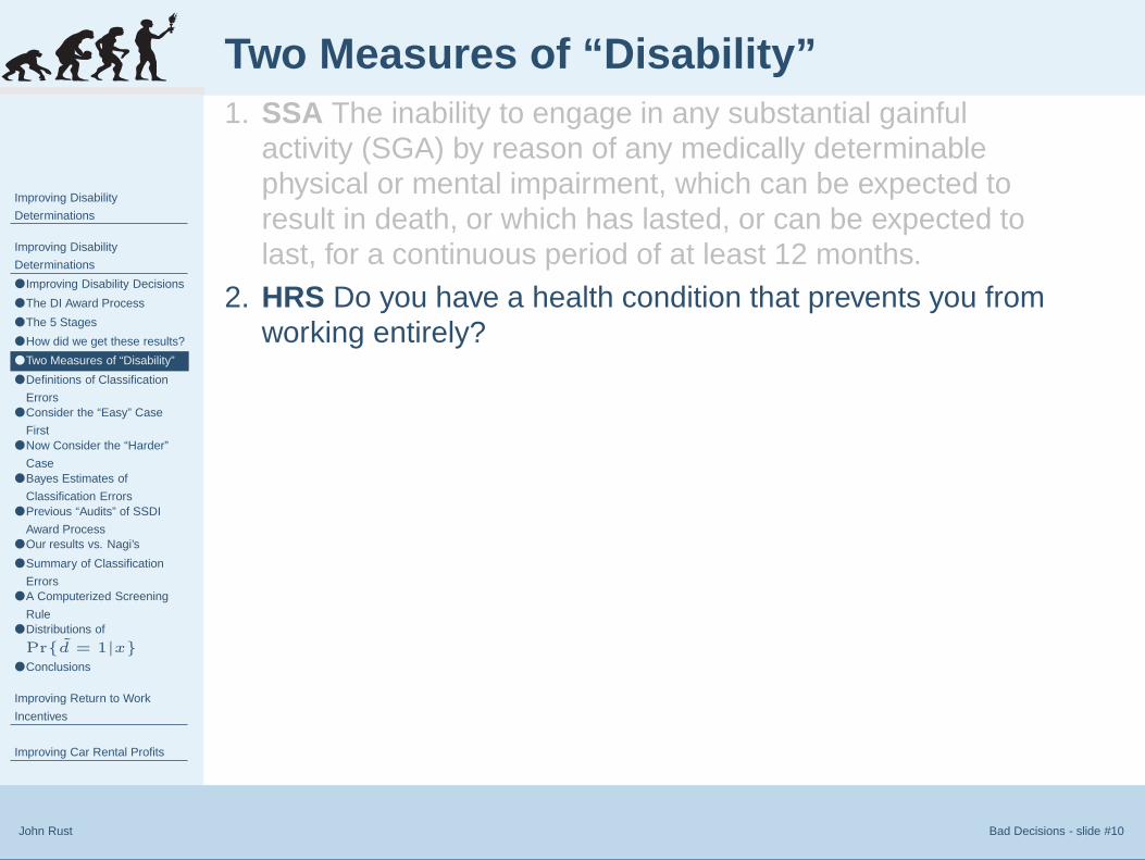
Improving Disability
Determinations
Improving Disability
Determinations
● Improving Disability Decisions
● The DI Award Process
● The 5 Stages
● How did we get these results?
● Two Measures of “Disability”
● Definitions of Classification
Errors● Consider the “Easy” Case
First● Now Consider the “Harder”
Case● Bayes Estimates of
Classification Errors● Previous “Audits” of SSDI
Award Process● Our results vs. Nagi’s
● Summary of Classification
Errors● A Computerized Screening
Rule● Distributions of
Pr{d = 1|x}● Conclusions
Improving Return to Work
Incentives
Improving Car Rental Profits
John Rust Bad Decisions - slide #10
Two Measures of “Disability”1. SSA The inability to engage in any substantial gainful
activity (SGA) by reason of any medically determinablephysical or mental impairment, which can be expected toresult in death, or which has lasted, or can be expected tolast, for a continuous period of at least 12 months.
2. HRS Do you have a health condition that prevents you fromworking entirely?

Improving Disability
Determinations
Improving Disability
Determinations
● Improving Disability Decisions
● The DI Award Process
● The 5 Stages
● How did we get these results?
● Two Measures of “Disability”
● Definitions of Classification
Errors● Consider the “Easy” Case
First● Now Consider the “Harder”
Case● Bayes Estimates of
Classification Errors● Previous “Audits” of SSDI
Award Process● Our results vs. Nagi’s
● Summary of Classification
Errors● A Computerized Screening
Rule● Distributions of
Pr{d = 1|x}● Conclusions
Improving Return to Work
Incentives
Improving Car Rental Profits
John Rust Bad Decisions - slide #10
Two Measures of “Disability”1. SSA The inability to engage in any substantial gainful
activity (SGA) by reason of any medically determinablephysical or mental impairment, which can be expected toresult in death, or which has lasted, or can be expected tolast, for a continuous period of at least 12 months.
2. HRS Do you have a health condition that prevents you fromworking entirely?
3. Define three binary random variables a, d and τ as follows:
a =
{1 if person is ultimately awarded SSDI/SSI benefits0 otherwise
d =
{1 if person reports they are unableto work0 otherwise
τ =
{1 if someone is “truly disabled”0 otherwise

Improving Disability
Determinations
Improving Disability
Determinations
● Improving Disability Decisions
● The DI Award Process
● The 5 Stages
● How did we get these results?
● Two Measures of “Disability”
● Definitions of Classification
Errors● Consider the “Easy” Case
First● Now Consider the “Harder”
Case● Bayes Estimates of
Classification Errors● Previous “Audits” of SSDI
Award Process● Our results vs. Nagi’s
● Summary of Classification
Errors● A Computerized Screening
Rule● Distributions of
Pr{d = 1|x}● Conclusions
Improving Return to Work
Incentives
Improving Car Rental Profits
John Rust Bad Decisions - slide #11
Definitions of Classification Errors
1. Award Error Rate This is the probability a person is nottruly disabled given that they are awarded benefits,Pr{τ = 0|a = 1}.
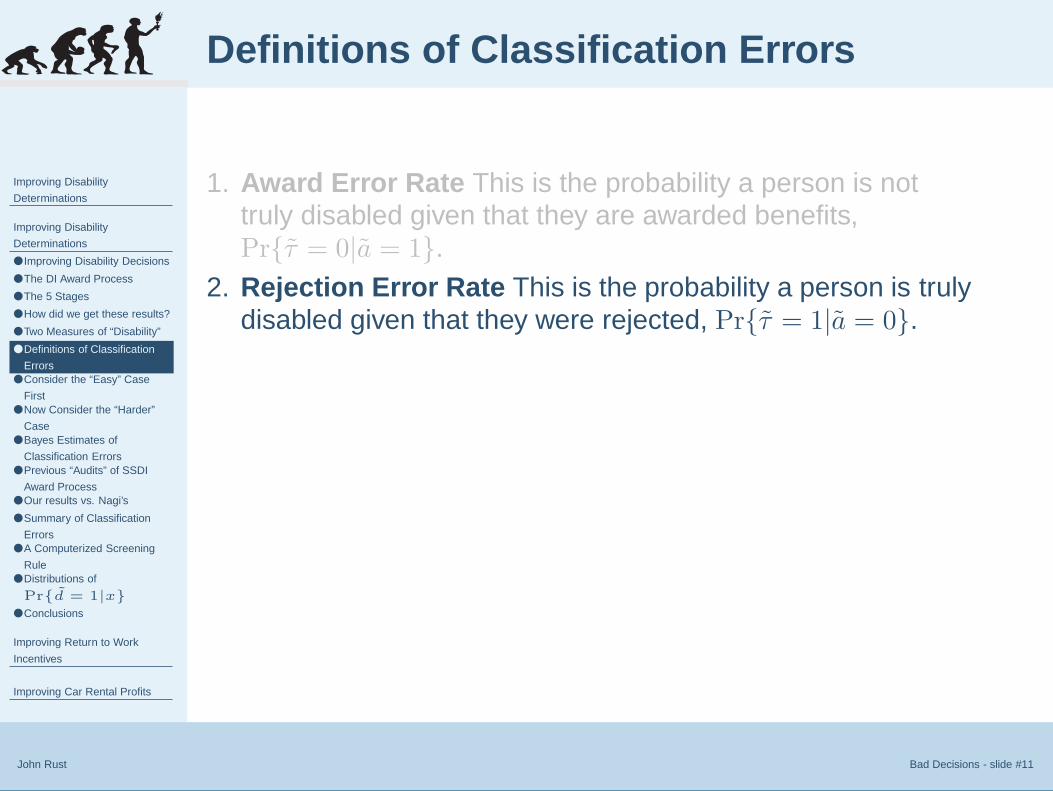
Improving Disability
Determinations
Improving Disability
Determinations
● Improving Disability Decisions
● The DI Award Process
● The 5 Stages
● How did we get these results?
● Two Measures of “Disability”
● Definitions of Classification
Errors● Consider the “Easy” Case
First● Now Consider the “Harder”
Case● Bayes Estimates of
Classification Errors● Previous “Audits” of SSDI
Award Process● Our results vs. Nagi’s
● Summary of Classification
Errors● A Computerized Screening
Rule● Distributions of
Pr{d = 1|x}● Conclusions
Improving Return to Work
Incentives
Improving Car Rental Profits
John Rust Bad Decisions - slide #11
Definitions of Classification Errors
1. Award Error Rate This is the probability a person is nottruly disabled given that they are awarded benefits,Pr{τ = 0|a = 1}.
2. Rejection Error Rate This is the probability a person is trulydisabled given that they were rejected, Pr{τ = 1|a = 0}.

Improving Disability
Determinations
Improving Disability
Determinations
● Improving Disability Decisions
● The DI Award Process
● The 5 Stages
● How did we get these results?
● Two Measures of “Disability”
● Definitions of Classification
Errors● Consider the “Easy” Case
First● Now Consider the “Harder”
Case● Bayes Estimates of
Classification Errors● Previous “Audits” of SSDI
Award Process● Our results vs. Nagi’s
● Summary of Classification
Errors● A Computerized Screening
Rule● Distributions of
Pr{d = 1|x}● Conclusions
Improving Return to Work
Incentives
Improving Car Rental Profits
John Rust Bad Decisions - slide #11
Definitions of Classification Errors
1. Award Error Rate This is the probability a person is nottruly disabled given that they are awarded benefits,Pr{τ = 0|a = 1}.
2. Rejection Error Rate This is the probability a person is trulydisabled given that they were rejected, Pr{τ = 1|a = 0}.
3. Note that the award and error rates differ from, but arerelated to, the Type I and II error rates in hypothesis testing.

Improving Disability
Determinations
Improving Disability
Determinations
● Improving Disability Decisions
● The DI Award Process
● The 5 Stages
● How did we get these results?
● Two Measures of “Disability”
● Definitions of Classification
Errors● Consider the “Easy” Case
First● Now Consider the “Harder”
Case● Bayes Estimates of
Classification Errors● Previous “Audits” of SSDI
Award Process● Our results vs. Nagi’s
● Summary of Classification
Errors● A Computerized Screening
Rule● Distributions of
Pr{d = 1|x}● Conclusions
Improving Return to Work
Incentives
Improving Car Rental Profits
John Rust Bad Decisions - slide #11
Definitions of Classification Errors
1. Award Error Rate This is the probability a person is nottruly disabled given that they are awarded benefits,Pr{τ = 0|a = 1}.
2. Rejection Error Rate This is the probability a person is trulydisabled given that they were rejected, Pr{τ = 1|a = 0}.
3. Note that the award and error rates differ from, but arerelated to, the Type I and II error rates in hypothesis testing.
4. Type I error rate the probability a person is rejected giventhat they are truly disabled, Pr{a = 0|τ = 1}

Improving Disability
Determinations
Improving Disability
Determinations
● Improving Disability Decisions
● The DI Award Process
● The 5 Stages
● How did we get these results?
● Two Measures of “Disability”
● Definitions of Classification
Errors● Consider the “Easy” Case
First● Now Consider the “Harder”
Case● Bayes Estimates of
Classification Errors● Previous “Audits” of SSDI
Award Process● Our results vs. Nagi’s
● Summary of Classification
Errors● A Computerized Screening
Rule● Distributions of
Pr{d = 1|x}● Conclusions
Improving Return to Work
Incentives
Improving Car Rental Profits
John Rust Bad Decisions - slide #11
Definitions of Classification Errors
1. Award Error Rate This is the probability a person is nottruly disabled given that they are awarded benefits,Pr{τ = 0|a = 1}.
2. Rejection Error Rate This is the probability a person is trulydisabled given that they were rejected, Pr{τ = 1|a = 0}.
3. Note that the award and error rates differ from, but arerelated to, the Type I and II error rates in hypothesis testing.
4. Type I error rate the probability a person is rejected giventhat they are truly disabled, Pr{a = 0|τ = 1}
5. Type II error rate the probability a person is accepted giventhat they are not truly disabled, Pr{a = 1|τ = 0}.

Improving Disability
Determinations
Improving Disability
Determinations
● Improving Disability Decisions
● The DI Award Process
● The 5 Stages
● How did we get these results?
● Two Measures of “Disability”
● Definitions of Classification
Errors● Consider the “Easy” Case
First● Now Consider the “Harder”
Case● Bayes Estimates of
Classification Errors● Previous “Audits” of SSDI
Award Process● Our results vs. Nagi’s
● Summary of Classification
Errors● A Computerized Screening
Rule● Distributions of
Pr{d = 1|x}● Conclusions
Improving Return to Work
Incentives
Improving Car Rental Profits
John Rust Bad Decisions - slide #12
Consider the “Easy” Case First
1. Suppose that τ = d with probability 1, i.e. that individualsknow and truthfully report their truly disability status, usingthe current “social standard” of disability for the currentsocio/political environment.
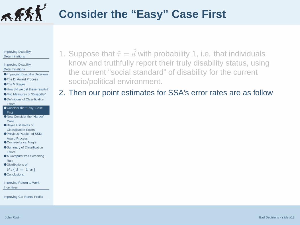
Improving Disability
Determinations
Improving Disability
Determinations
● Improving Disability Decisions
● The DI Award Process
● The 5 Stages
● How did we get these results?
● Two Measures of “Disability”
● Definitions of Classification
Errors● Consider the “Easy” Case
First● Now Consider the “Harder”
Case● Bayes Estimates of
Classification Errors● Previous “Audits” of SSDI
Award Process● Our results vs. Nagi’s
● Summary of Classification
Errors● A Computerized Screening
Rule● Distributions of
Pr{d = 1|x}● Conclusions
Improving Return to Work
Incentives
Improving Car Rental Profits
John Rust Bad Decisions - slide #12
Consider the “Easy” Case First
1. Suppose that τ = d with probability 1, i.e. that individualsknow and truthfully report their truly disability status, usingthe current “social standard” of disability for the currentsocio/political environment.
2. Then our point estimates for SSA’s error rates are as follow

Improving Disability
Determinations
Improving Disability
Determinations
● Improving Disability Decisions
● The DI Award Process
● The 5 Stages
● How did we get these results?
● Two Measures of “Disability”
● Definitions of Classification
Errors● Consider the “Easy” Case
First● Now Consider the “Harder”
Case● Bayes Estimates of
Classification Errors● Previous “Audits” of SSDI
Award Process● Our results vs. Nagi’s
● Summary of Classification
Errors● A Computerized Screening
Rule● Distributions of
Pr{d = 1|x}● Conclusions
Improving Return to Work
Incentives
Improving Car Rental Profits
John Rust Bad Decisions - slide #12
Consider the “Easy” Case First
1. Suppose that τ = d with probability 1, i.e. that individualsknow and truthfully report their truly disability status, usingthe current “social standard” of disability for the currentsocio/political environment.
2. Then our point estimates for SSA’s error rates are as follow
3. Award Error Rate Pr{d = 0|a = 1} = .28
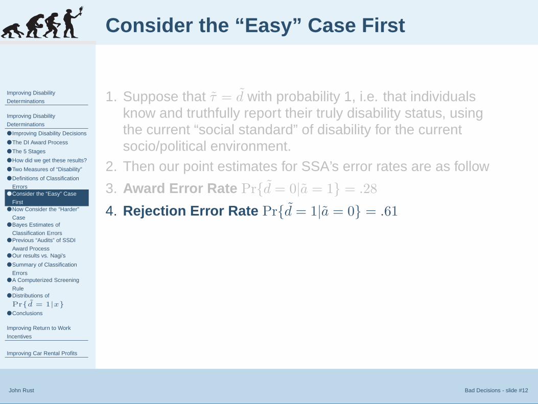
Improving Disability
Determinations
Improving Disability
Determinations
● Improving Disability Decisions
● The DI Award Process
● The 5 Stages
● How did we get these results?
● Two Measures of “Disability”
● Definitions of Classification
Errors● Consider the “Easy” Case
First● Now Consider the “Harder”
Case● Bayes Estimates of
Classification Errors● Previous “Audits” of SSDI
Award Process● Our results vs. Nagi’s
● Summary of Classification
Errors● A Computerized Screening
Rule● Distributions of
Pr{d = 1|x}● Conclusions
Improving Return to Work
Incentives
Improving Car Rental Profits
John Rust Bad Decisions - slide #12
Consider the “Easy” Case First
1. Suppose that τ = d with probability 1, i.e. that individualsknow and truthfully report their truly disability status, usingthe current “social standard” of disability for the currentsocio/political environment.
2. Then our point estimates for SSA’s error rates are as follow
3. Award Error Rate Pr{d = 0|a = 1} = .28
4. Rejection Error Rate Pr{d = 1|a = 0} = .61

Improving Disability
Determinations
Improving Disability
Determinations
● Improving Disability Decisions
● The DI Award Process
● The 5 Stages
● How did we get these results?
● Two Measures of “Disability”
● Definitions of Classification
Errors● Consider the “Easy” Case
First● Now Consider the “Harder”
Case● Bayes Estimates of
Classification Errors● Previous “Audits” of SSDI
Award Process● Our results vs. Nagi’s
● Summary of Classification
Errors● A Computerized Screening
Rule● Distributions of
Pr{d = 1|x}● Conclusions
Improving Return to Work
Incentives
Improving Car Rental Profits
John Rust Bad Decisions - slide #12
Consider the “Easy” Case First
1. Suppose that τ = d with probability 1, i.e. that individualsknow and truthfully report their truly disability status, usingthe current “social standard” of disability for the currentsocio/political environment.
2. Then our point estimates for SSA’s error rates are as follow
3. Award Error Rate Pr{d = 0|a = 1} = .28
4. Rejection Error Rate Pr{d = 1|a = 0} = .61
5. Type I Error Rate Pr{a = 0|d = 1} = .26
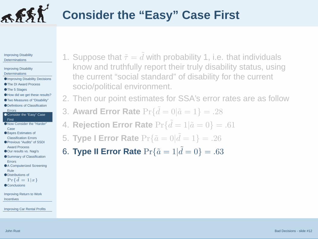
Improving Disability
Determinations
Improving Disability
Determinations
● Improving Disability Decisions
● The DI Award Process
● The 5 Stages
● How did we get these results?
● Two Measures of “Disability”
● Definitions of Classification
Errors● Consider the “Easy” Case
First● Now Consider the “Harder”
Case● Bayes Estimates of
Classification Errors● Previous “Audits” of SSDI
Award Process● Our results vs. Nagi’s
● Summary of Classification
Errors● A Computerized Screening
Rule● Distributions of
Pr{d = 1|x}● Conclusions
Improving Return to Work
Incentives
Improving Car Rental Profits
John Rust Bad Decisions - slide #12
Consider the “Easy” Case First
1. Suppose that τ = d with probability 1, i.e. that individualsknow and truthfully report their truly disability status, usingthe current “social standard” of disability for the currentsocio/political environment.
2. Then our point estimates for SSA’s error rates are as follow
3. Award Error Rate Pr{d = 0|a = 1} = .28
4. Rejection Error Rate Pr{d = 1|a = 0} = .61
5. Type I Error Rate Pr{a = 0|d = 1} = .26
6. Type II Error Rate Pr{a = 1|d = 0} = .63
Improving Disability
Determinations
Improving Disability
Determinations
● Improving Disability Decisions
● The DI Award Process
● The 5 Stages
● How did we get these results?
● Two Measures of “Disability”
● Definitions of Classification
Errors● Consider the “Easy” Case
First● Now Consider the “Harder”
Case● Bayes Estimates of
Classification Errors● Previous “Audits” of SSDI
Award Process● Our results vs. Nagi’s
● Summary of Classification
Errors● A Computerized Screening
Rule● Distributions of
Pr{d = 1|x}● Conclusions
Improving Return to Work
Incentives
Improving Car Rental Profits
John Rust Bad Decisions - slide #13
Now Consider the “Harder” Case
1. Assume that both a and d are noisy but unbiased indicatorsof true disability status τ

Improving Disability
Determinations
Improving Disability
Determinations
● Improving Disability Decisions
● The DI Award Process
● The 5 Stages
● How did we get these results?
● Two Measures of “Disability”
● Definitions of Classification
Errors● Consider the “Easy” Case
First● Now Consider the “Harder”
Case● Bayes Estimates of
Classification Errors● Previous “Audits” of SSDI
Award Process● Our results vs. Nagi’s
● Summary of Classification
Errors● A Computerized Screening
Rule● Distributions of
Pr{d = 1|x}● Conclusions
Improving Return to Work
Incentives
Improving Car Rental Profits
John Rust Bad Decisions - slide #13
Now Consider the “Harder” Case
1. Assume that both a and d are noisy but unbiased indicatorsof true disability status τ
2. Assume that we can model (a, d, τ) as a trivariate probit witha correlation structure designed to match the correlationbetween the observed random variables a and d.
Improving Disability
Determinations
Improving Disability
Determinations
● Improving Disability Decisions
● The DI Award Process
● The 5 Stages
● How did we get these results?
● Two Measures of “Disability”
● Definitions of Classification
Errors● Consider the “Easy” Case
First● Now Consider the “Harder”
Case● Bayes Estimates of
Classification Errors● Previous “Audits” of SSDI
Award Process● Our results vs. Nagi’s
● Summary of Classification
Errors● A Computerized Screening
Rule● Distributions of
Pr{d = 1|x}● Conclusions
Improving Return to Work
Incentives
Improving Car Rental Profits
John Rust Bad Decisions - slide #13
Now Consider the “Harder” Case
1. Assume that both a and d are noisy but unbiased indicatorsof true disability status τ
2. Assume that we can model (a, d, τ) as a trivariate probit witha correlation structure designed to match the correlationbetween the observed random variables a and d.
3. Under these assumptions we can estimate the parametersof the trivariate probit model by maximum likelihood and usethe resulting model to infer the classification and Type I andII error rates using Bayes Rule.
Improving Disability
Determinations
Improving Disability
Determinations
● Improving Disability Decisions
● The DI Award Process
● The 5 Stages
● How did we get these results?
● Two Measures of “Disability”
● Definitions of Classification
Errors● Consider the “Easy” Case
First● Now Consider the “Harder”
Case● Bayes Estimates of
Classification Errors● Previous “Audits” of SSDI
Award Process● Our results vs. Nagi’s
● Summary of Classification
Errors● A Computerized Screening
Rule● Distributions of
Pr{d = 1|x}● Conclusions
Improving Return to Work
Incentives
Improving Car Rental Profits
John Rust Bad Decisions - slide #13
Now Consider the “Harder” Case
1. Assume that both a and d are noisy but unbiased indicatorsof true disability status τ
2. Assume that we can model (a, d, τ) as a trivariate probit witha correlation structure designed to match the correlationbetween the observed random variables a and d.
3. Under these assumptions we can estimate the parametersof the trivariate probit model by maximum likelihood and usethe resulting model to infer the classification and Type I andII error rates using Bayes Rule.
4. Surprisingly, when we do these computations in this morerealistic case, the rate of classification errors and the Type Iand II error rates differ by only a small amount from the errorrates we obtained in the “easy” case when we assumed thatd = τ .

Improving Disability
Determinations
Improving Disability
Determinations
● Improving Disability Decisions
● The DI Award Process
● The 5 Stages
● How did we get these results?
● Two Measures of “Disability”
● Definitions of Classification
Errors● Consider the “Easy” Case
First● Now Consider the “Harder”
Case● Bayes Estimates of
Classification Errors● Previous “Audits” of SSDI
Award Process● Our results vs. Nagi’s
● Summary of Classification
Errors● A Computerized Screening
Rule● Distributions of
Pr{d = 1|x}● Conclusions
Improving Return to Work
Incentives
Improving Car Rental Profits
John Rust Bad Decisions - slide #14
Bayes Estimates of Classification Errors
1. Award Error Rate: Pr{d = 0|a = 1} = .23

Improving Disability
Determinations
Improving Disability
Determinations
● Improving Disability Decisions
● The DI Award Process
● The 5 Stages
● How did we get these results?
● Two Measures of “Disability”
● Definitions of Classification
Errors● Consider the “Easy” Case
First● Now Consider the “Harder”
Case● Bayes Estimates of
Classification Errors● Previous “Audits” of SSDI
Award Process● Our results vs. Nagi’s
● Summary of Classification
Errors● A Computerized Screening
Rule● Distributions of
Pr{d = 1|x}● Conclusions
Improving Return to Work
Incentives
Improving Car Rental Profits
John Rust Bad Decisions - slide #14
Bayes Estimates of Classification Errors
1. Award Error Rate: Pr{d = 0|a = 1} = .23
2. Rejection Error Rate Pr{d = 1|a = 0} = .61

Improving Disability
Determinations
Improving Disability
Determinations
● Improving Disability Decisions
● The DI Award Process
● The 5 Stages
● How did we get these results?
● Two Measures of “Disability”
● Definitions of Classification
Errors● Consider the “Easy” Case
First● Now Consider the “Harder”
Case● Bayes Estimates of
Classification Errors● Previous “Audits” of SSDI
Award Process● Our results vs. Nagi’s
● Summary of Classification
Errors● A Computerized Screening
Rule● Distributions of
Pr{d = 1|x}● Conclusions
Improving Return to Work
Incentives
Improving Car Rental Profits
John Rust Bad Decisions - slide #14
Bayes Estimates of Classification Errors
1. Award Error Rate: Pr{d = 0|a = 1} = .23
2. Rejection Error Rate Pr{d = 1|a = 0} = .61
3. Type I Error Rate Pr{a = 0|d = 1} = .23

Improving Disability
Determinations
Improving Disability
Determinations
● Improving Disability Decisions
● The DI Award Process
● The 5 Stages
● How did we get these results?
● Two Measures of “Disability”
● Definitions of Classification
Errors● Consider the “Easy” Case
First● Now Consider the “Harder”
Case● Bayes Estimates of
Classification Errors● Previous “Audits” of SSDI
Award Process● Our results vs. Nagi’s
● Summary of Classification
Errors● A Computerized Screening
Rule● Distributions of
Pr{d = 1|x}● Conclusions
Improving Return to Work
Incentives
Improving Car Rental Profits
John Rust Bad Decisions - slide #14
Bayes Estimates of Classification Errors
1. Award Error Rate: Pr{d = 0|a = 1} = .23
2. Rejection Error Rate Pr{d = 1|a = 0} = .61
3. Type I Error Rate Pr{a = 0|d = 1} = .23
4. Type II Error Rate Pr{a = 1|d = 0} = .68
Improving Disability
Determinations
Improving Disability
Determinations
● Improving Disability Decisions
● The DI Award Process
● The 5 Stages
● How did we get these results?
● Two Measures of “Disability”
● Definitions of Classification
Errors● Consider the “Easy” Case
First● Now Consider the “Harder”
Case● Bayes Estimates of
Classification Errors● Previous “Audits” of SSDI
Award Process● Our results vs. Nagi’s
● Summary of Classification
Errors● A Computerized Screening
Rule● Distributions of
Pr{d = 1|x}● Conclusions
Improving Return to Work
Incentives
Improving Car Rental Profits
John Rust Bad Decisions - slide #15
Previous “Audits” of SSDI Award Process
1. These studies provide similar estimates of classificationerror rates using very different methologies

Improving Disability
Determinations
Improving Disability
Determinations
● Improving Disability Decisions
● The DI Award Process
● The 5 Stages
● How did we get these results?
● Two Measures of “Disability”
● Definitions of Classification
Errors● Consider the “Easy” Case
First● Now Consider the “Harder”
Case● Bayes Estimates of
Classification Errors● Previous “Audits” of SSDI
Award Process● Our results vs. Nagi’s
● Summary of Classification
Errors● A Computerized Screening
Rule● Distributions of
Pr{d = 1|x}● Conclusions
Improving Return to Work
Incentives
Improving Car Rental Profits
John Rust Bad Decisions - slide #15
Previous “Audits” of SSDI Award Process
1. These studies provide similar estimates of classificationerror rates using very different methologies
2. Nagi (1969) compared an “expert decision” (a moderatedgroup decision of an examining team consisting of aphysician, psychologist, social worker, occupationaltherapist, and a vocational rehabilitation expert) to SSA’saward decision
Expert SSA Award Decision TotalTeam Decision Awarded Denied
Can Work 291 492 783(19.3%) (52.1%) (31.9%)
Cannot Work 1,219 452 1,671(80.7%) (47.9%) (68.1%)
Total 1,510 944 2,454(61.5%) (38.5%) (100.0%)

Improving Disability
Determinations
Improving Disability
Determinations
● Improving Disability Decisions
● The DI Award Process
● The 5 Stages
● How did we get these results?
● Two Measures of “Disability”
● Definitions of Classification
Errors● Consider the “Easy” Case
First● Now Consider the “Harder”
Case● Bayes Estimates of
Classification Errors● Previous “Audits” of SSDI
Award Process● Our results vs. Nagi’s
● Summary of Classification
Errors● A Computerized Screening
Rule● Distributions of
Pr{d = 1|x}● Conclusions
Improving Return to Work
Incentives
Improving Car Rental Profits
John Rust Bad Decisions - slide #16
Our results vs. Nagi’s
1. We analyzed a subsample of 360 HRS respondents forwhich complete information on ADLs and healthcharacteristics are available

Improving Disability
Determinations
Improving Disability
Determinations
● Improving Disability Decisions
● The DI Award Process
● The 5 Stages
● How did we get these results?
● Two Measures of “Disability”
● Definitions of Classification
Errors● Consider the “Easy” Case
First● Now Consider the “Harder”
Case● Bayes Estimates of
Classification Errors● Previous “Audits” of SSDI
Award Process● Our results vs. Nagi’s
● Summary of Classification
Errors● A Computerized Screening
Rule● Distributions of
Pr{d = 1|x}● Conclusions
Improving Return to Work
Incentives
Improving Car Rental Profits
John Rust Bad Decisions - slide #16
Our results vs. Nagi’s
1. We analyzed a subsample of 360 HRS respondents forwhich complete information on ADLs and healthcharacteristics are available
2. We don’t have access to an independent expert, so wecompare self-reported disability to SSA’s award decision
Self-Reported SSA Award Decision TotalDisability Status Awarded Denied
Not Disabled 60 42 102(22.6%) (44.7%) (28.3%)
Disabled 206 52 258(77.4%) (55.3%) (71.7%)
Total 266 94 360(73.9%) (26.1%) (100.0%)
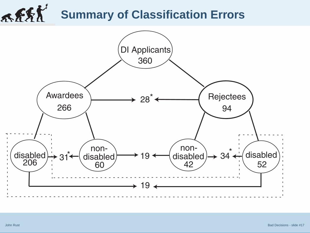
John Rust Bad Decisions - slide #17
Summary of Classification Errors
Awardees Rejectees
DI Applicants
disabled disableddisabled disablednon- non-
28*
31*
19
34*
360
266 94
60 5242 19
206

Improving Disability
Determinations
Improving Disability
Determinations
● Improving Disability Decisions
● The DI Award Process
● The 5 Stages
● How did we get these results?
● Two Measures of “Disability”
● Definitions of Classification
Errors● Consider the “Easy” Case
First● Now Consider the “Harder”
Case● Bayes Estimates of
Classification Errors● Previous “Audits” of SSDI
Award Process● Our results vs. Nagi’s
● Summary of Classification
Errors● A Computerized Screening
Rule● Distributions of
Pr{d = 1|x}● Conclusions
Improving Return to Work
Incentives
Improving Car Rental Profits
John Rust Bad Decisions - slide #18
A Computerized Screening Rule1. Even if we believe that self-reported disability status d is
truthfully reported in an anonymous survey such as HRS,SSDI/SSI applicants have a clear incentive to lie about theirdisability status to the SSA

Improving Disability
Determinations
Improving Disability
Determinations
● Improving Disability Decisions
● The DI Award Process
● The 5 Stages
● How did we get these results?
● Two Measures of “Disability”
● Definitions of Classification
Errors● Consider the “Easy” Case
First● Now Consider the “Harder”
Case● Bayes Estimates of
Classification Errors● Previous “Audits” of SSDI
Award Process● Our results vs. Nagi’s
● Summary of Classification
Errors● A Computerized Screening
Rule● Distributions of
Pr{d = 1|x}● Conclusions
Improving Return to Work
Incentives
Improving Car Rental Profits
John Rust Bad Decisions - slide #18
A Computerized Screening Rule1. Even if we believe that self-reported disability status d is
truthfully reported in an anonymous survey such as HRS,SSDI/SSI applicants have a clear incentive to lie about theirdisability status to the SSA
2. However we can use the HRS data to regress d against avector x of “objective” health conditions and ADLs, such as“do you have heart problems?” “do you have diabetes?”“have you had a stroke?” etc.

Improving Disability
Determinations
Improving Disability
Determinations
● Improving Disability Decisions
● The DI Award Process
● The 5 Stages
● How did we get these results?
● Two Measures of “Disability”
● Definitions of Classification
Errors● Consider the “Easy” Case
First● Now Consider the “Harder”
Case● Bayes Estimates of
Classification Errors● Previous “Audits” of SSDI
Award Process● Our results vs. Nagi’s
● Summary of Classification
Errors● A Computerized Screening
Rule● Distributions of
Pr{d = 1|x}● Conclusions
Improving Return to Work
Incentives
Improving Car Rental Profits
John Rust Bad Decisions - slide #18
A Computerized Screening Rule1. Even if we believe that self-reported disability status d is
truthfully reported in an anonymous survey such as HRS,SSDI/SSI applicants have a clear incentive to lie about theirdisability status to the SSA
2. However we can use the HRS data to regress d against avector x of “objective” health conditions and ADLs, such as“do you have heart problems?” “do you have diabetes?”“have you had a stroke?” etc.
3. Using the HRS data we then can compute predictedprobabilities that a person is truly disabled. These predictedprobabilities depend only on the observablehealth/demographic characteristics
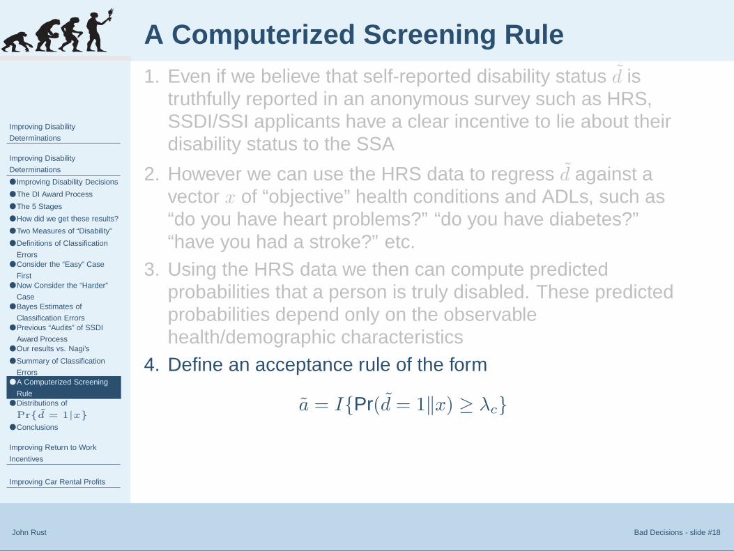
Improving Disability
Determinations
Improving Disability
Determinations
● Improving Disability Decisions
● The DI Award Process
● The 5 Stages
● How did we get these results?
● Two Measures of “Disability”
● Definitions of Classification
Errors● Consider the “Easy” Case
First● Now Consider the “Harder”
Case● Bayes Estimates of
Classification Errors● Previous “Audits” of SSDI
Award Process● Our results vs. Nagi’s
● Summary of Classification
Errors● A Computerized Screening
Rule● Distributions of
Pr{d = 1|x}● Conclusions
Improving Return to Work
Incentives
Improving Car Rental Profits
John Rust Bad Decisions - slide #18
A Computerized Screening Rule1. Even if we believe that self-reported disability status d is
truthfully reported in an anonymous survey such as HRS,SSDI/SSI applicants have a clear incentive to lie about theirdisability status to the SSA
2. However we can use the HRS data to regress d against avector x of “objective” health conditions and ADLs, such as“do you have heart problems?” “do you have diabetes?”“have you had a stroke?” etc.
3. Using the HRS data we then can compute predictedprobabilities that a person is truly disabled. These predictedprobabilities depend only on the observablehealth/demographic characteristics
4. Define an acceptance rule of the form
a = I{Pr(d = 1‖x) ≥ λc}

Improving Disability
Determinations
Improving Disability
Determinations
● Improving Disability Decisions
● The DI Award Process
● The 5 Stages
● How did we get these results?
● Two Measures of “Disability”
● Definitions of Classification
Errors● Consider the “Easy” Case
First● Now Consider the “Harder”
Case● Bayes Estimates of
Classification Errors● Previous “Audits” of SSDI
Award Process● Our results vs. Nagi’s
● Summary of Classification
Errors● A Computerized Screening
Rule● Distributions of
Pr{d = 1|x}● Conclusions
Improving Return to Work
Incentives
Improving Car Rental Profits
John Rust Bad Decisions - slide #18
A Computerized Screening Rule1. Even if we believe that self-reported disability status d is
truthfully reported in an anonymous survey such as HRS,SSDI/SSI applicants have a clear incentive to lie about theirdisability status to the SSA
2. However we can use the HRS data to regress d against avector x of “objective” health conditions and ADLs, such as“do you have heart problems?” “do you have diabetes?”“have you had a stroke?” etc.
3. Using the HRS data we then can compute predictedprobabilities that a person is truly disabled. These predictedprobabilities depend only on the observablehealth/demographic characteristics
4. Define an acceptance rule of the form
a = I{Pr(d = 1‖x) ≥ λc}
5. By varying the cutoff λc we can achieve any desired awardrate.


Improving Disability
Determinations
Improving Disability
Determinations
● Improving Disability Decisions
● The DI Award Process
● The 5 Stages
● How did we get these results?
● Two Measures of “Disability”
● Definitions of Classification
Errors● Consider the “Easy” Case
First● Now Consider the “Harder”
Case● Bayes Estimates of
Classification Errors● Previous “Audits” of SSDI
Award Process● Our results vs. Nagi’s
● Summary of Classification
Errors● A Computerized Screening
Rule● Distributions of
Pr{d = 1|x}● Conclusions
Improving Return to Work
Incentives
Improving Car Rental Profits
John Rust Bad Decisions - slide #20
Conclusions
1. We have shown that the SSDI/SSI award process used bythe SSA is very noisy, resulting in award error rates of over20% and rejection error rates of over 50%
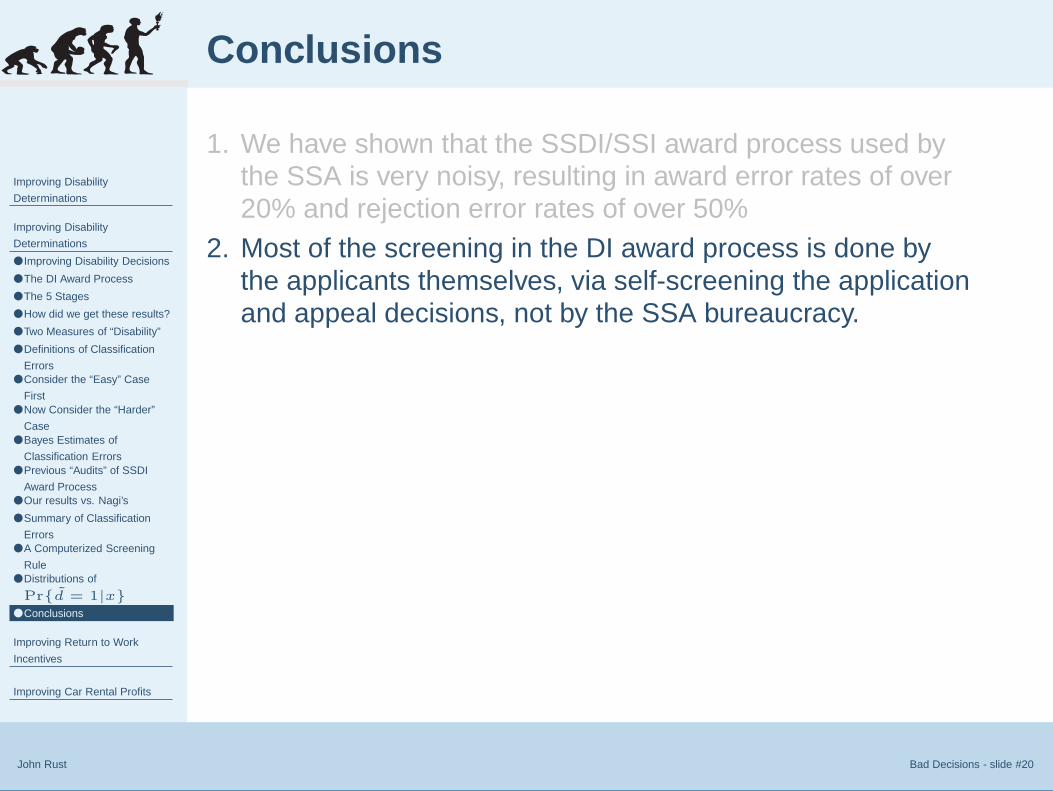
Improving Disability
Determinations
Improving Disability
Determinations
● Improving Disability Decisions
● The DI Award Process
● The 5 Stages
● How did we get these results?
● Two Measures of “Disability”
● Definitions of Classification
Errors● Consider the “Easy” Case
First● Now Consider the “Harder”
Case● Bayes Estimates of
Classification Errors● Previous “Audits” of SSDI
Award Process● Our results vs. Nagi’s
● Summary of Classification
Errors● A Computerized Screening
Rule● Distributions of
Pr{d = 1|x}● Conclusions
Improving Return to Work
Incentives
Improving Car Rental Profits
John Rust Bad Decisions - slide #20
Conclusions
1. We have shown that the SSDI/SSI award process used bythe SSA is very noisy, resulting in award error rates of over20% and rejection error rates of over 50%
2. Most of the screening in the DI award process is done bythe applicants themselves, via self-screening the applicationand appeal decisions, not by the SSA bureaucracy.

Improving Disability
Determinations
Improving Disability
Determinations
● Improving Disability Decisions
● The DI Award Process
● The 5 Stages
● How did we get these results?
● Two Measures of “Disability”
● Definitions of Classification
Errors● Consider the “Easy” Case
First● Now Consider the “Harder”
Case● Bayes Estimates of
Classification Errors● Previous “Audits” of SSDI
Award Process● Our results vs. Nagi’s
● Summary of Classification
Errors● A Computerized Screening
Rule● Distributions of
Pr{d = 1|x}● Conclusions
Improving Return to Work
Incentives
Improving Car Rental Profits
John Rust Bad Decisions - slide #20
Conclusions
1. We have shown that the SSDI/SSI award process used bythe SSA is very noisy, resulting in award error rates of over20% and rejection error rates of over 50%
2. Most of the screening in the DI award process is done bythe applicants themselves, via self-screening the applicationand appeal decisions, not by the SSA bureaucracy.
3. The first stage decisions by the DDSs have low award ratesand extremely high rates of rejection error. They appear tobe adopting a strategy of “when in doubt, reject”

Improving Disability
Determinations
Improving Disability
Determinations
● Improving Disability Decisions
● The DI Award Process
● The 5 Stages
● How did we get these results?
● Two Measures of “Disability”
● Definitions of Classification
Errors● Consider the “Easy” Case
First● Now Consider the “Harder”
Case● Bayes Estimates of
Classification Errors● Previous “Audits” of SSDI
Award Process● Our results vs. Nagi’s
● Summary of Classification
Errors● A Computerized Screening
Rule● Distributions of
Pr{d = 1|x}● Conclusions
Improving Return to Work
Incentives
Improving Car Rental Profits
John Rust Bad Decisions - slide #20
Conclusions
1. We have shown that the SSDI/SSI award process used bythe SSA is very noisy, resulting in award error rates of over20% and rejection error rates of over 50%
2. Most of the screening in the DI award process is done bythe applicants themselves, via self-screening the applicationand appeal decisions, not by the SSA bureaucracy.
3. The first stage decisions by the DDSs have low award ratesand extremely high rates of rejection error. They appear tobe adopting a strategy of “when in doubt, reject”
4. Contrary to the GAO analysis, we find that the appeal stageto the ALJs, and the high rate of reversals, substantiallyreduces the rate of rejection errors without increasing therate of award errors.

John Rust Bad Decisions - slide #21
Improving Return to Work Incentives

Improving Disability
Determinations
Improving Return to Work
Incentives
Improving Returen to Work
Incentives
● Measuring “Induced Entry
Effects”● The Concern about Induced
Entry● Problems with Randomized
Experiments
● A Life Cycle Model
● Simulated vs. Population
Survival Rates● Simulated vs. Actual Health
Status● A Life Cycle Model, continued
● Weights on Leisure by Age
and Average Wage
● Simulated vs. Actual Labor
Supply
● Simulated vs. Actual Social
Security Receipt
● Simulated vs. Actual Social
Security Status
● Simulated vs. Actual Net
Worth● Consumption, Wages and DI
Receipt
● Bequests, IRR on Social
Security● Impact on DI Applications and
Rolls● Impact on Labor Supply
● Impact on Wages and Taxes
● Impact on Social Security
● Impact on Wealth and
John Rust Bad Decisions - slide #22
Measuring “Induced Entry Effects”1. Joint work with Hugo Benitez and Moshe Buchinsky that
originated in 1999, when I was appointed as an advisor tothe Social Security Administration
2. part of a committee charged with designing an experimentto measure induced entry effects of the “$1 for $2 offset”, aprovision in the 1999 Ticket to Work and Work IncentivesImprovement Act signed by President Clinton.
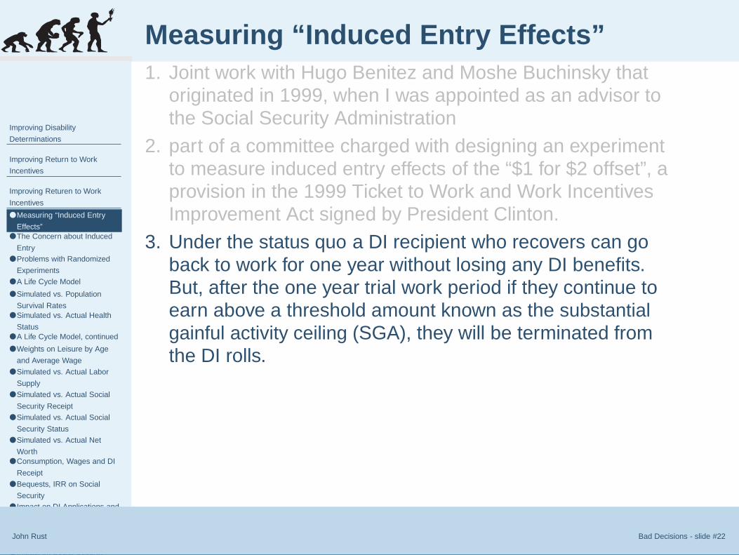
3. Under the status quo a DI recipient who recovers can goback to work for one year without losing any DI benefits.But, after the one year trial work period if they continue toearn above a threshold amount known as the substantialgainful activity ceiling (SGA), they will be terminated fromthe DI rolls.
4. Under the $1 for $2 offset, DI recipients can work andremain on DI, but they lose $1 of DI benefits for every $2earned above the SGA threshold (about$9000 per year).
5. The 1999 law enabled SSA to conduct randomizedexperiments designed to measure the induced entry effect.
Improving Disability
Determinations
Improving Return to Work
Incentives
Improving Returen to Work
Incentives
● Measuring “Induced Entry
Effects”● The Concern about Induced
Entry● Problems with Randomized
Experiments
● A Life Cycle Model
● Simulated vs. Population
Survival Rates● Simulated vs. Actual Health
Status● A Life Cycle Model, continued
● Weights on Leisure by Age
and Average Wage
● Simulated vs. Actual Labor
Supply
● Simulated vs. Actual Social
Security Receipt
● Simulated vs. Actual Social
Security Status
● Simulated vs. Actual Net
Worth● Consumption, Wages and DI
Receipt
● Bequests, IRR on Social
Security● Impact on DI Applications and
Rolls● Impact on Labor Supply
● Impact on Wages and Taxes
● Impact on Social Security
● Impact on Wealth and
John Rust Bad Decisions - slide #23
The Concern about Induced Entry
1. The $1 for $2 offset reduces the 100% effective tax rate onDI benefits from going back to work after the trial workperiod
2. Advocates for DI beneficiaries argued that under the lower50% effective tax rate under the $1 for $2 offset, we shouldexpected to see more labor supply and even induced exitfrom DI.
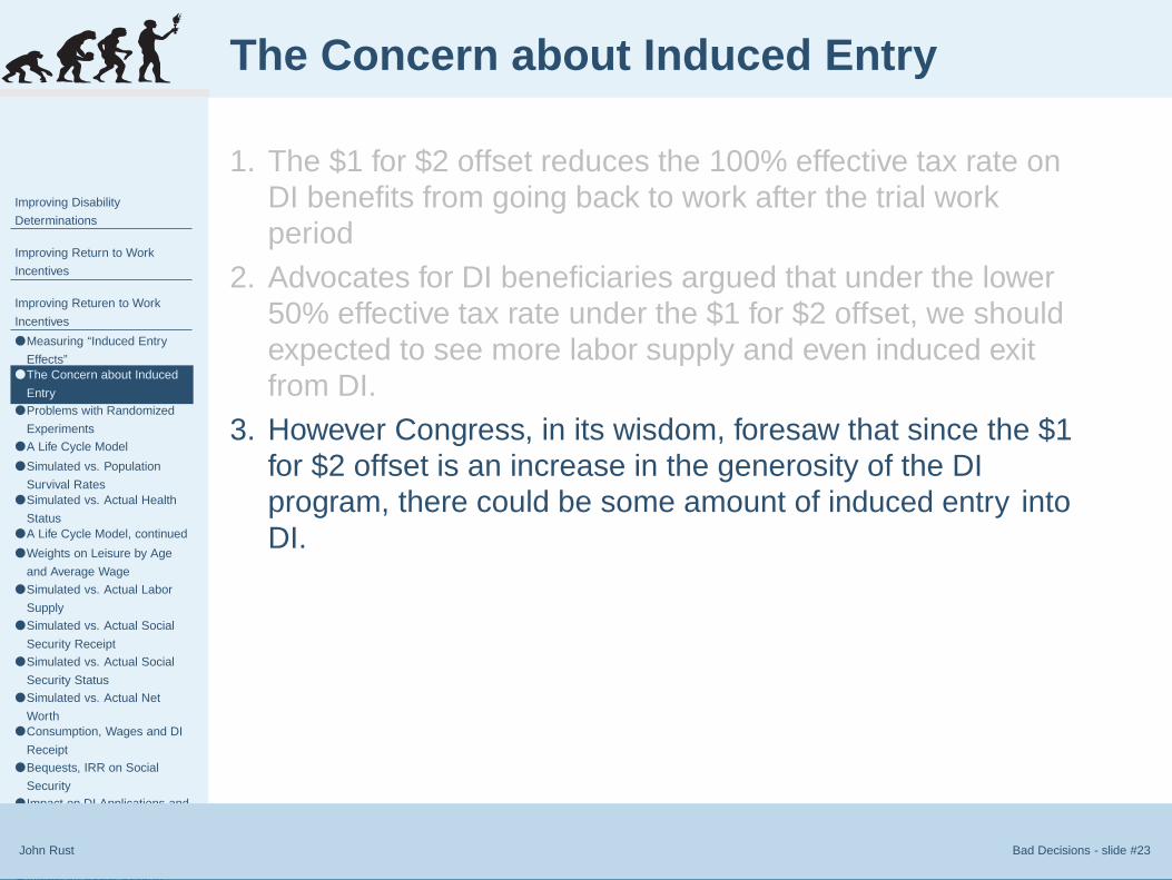
3. However Congress, in its wisdom, foresaw that since the $1for $2 offset is an increase in the generosity of the DIprogram, there could be some amount of induced entry intoDI.
4. Would the decreased costs due to “induced exit” from DIoutweigh the increase in costs due to “induced entry”?
5. Congress mandated that a randomized experiment beconducted to answer this question and assess the costeffectiveness of the $1 for $2 offset.

Improving Disability
Determinations
Improving Return to Work
Incentives
Improving Returen to Work
Incentives
● Measuring “Induced Entry
Effects”● The Concern about Induced
Entry● Problems with Randomized
Experiments
● A Life Cycle Model
● Simulated vs. Population
Survival Rates● Simulated vs. Actual Health
Status● A Life Cycle Model, continued
● Weights on Leisure by Age
and Average Wage
● Simulated vs. Actual Labor
Supply
● Simulated vs. Actual Social
Security Receipt
● Simulated vs. Actual Social
Security Status
● Simulated vs. Actual Net
Worth● Consumption, Wages and DI
Receipt
● Bequests, IRR on Social
Security● Impact on DI Applications and
Rolls● Impact on Labor Supply
● Impact on Wages and Taxes
● Impact on Social Security
● Impact on Wealth and
John Rust Bad Decisions - slide #24
Problems with Randomized Experiments1. Applications for disability take place in a community/social
context. Doctors’, friends’, and bureaucrats’ knowledge ofthe disability program can affect an individual’s decision toapply for DI.
2. Thus, the committee of experts felt that potential DIapplicants were randomly selected into the “treatmentgroup” of those eligible for the $1 for $2 offset.
3. Instead, in order to get an accurate assessment, entirecommunities (counties) would have to selected for inclusionin the treatment group.
4. But since there are very large geographic variations in DIapplication and award rates, and in overall economicconditions in the county, large numbers of counties wouldhave to be included in the treatment and control groups.
5. This means that potentionally millions of people would beliving in counties that were randomly selected into thetreatment group of counties whose citizens are eligible forthe $1 for $2 offset.

Improving Disability
Determinations
Improving Return to Work
Incentives
Improving Returen to Work
Incentives
● Measuring “Induced Entry
Effects”● The Concern about Induced
Entry● Problems with Randomized
Experiments
● A Life Cycle Model
● Simulated vs. Population
Survival Rates● Simulated vs. Actual Health
Status● A Life Cycle Model, continued
● Weights on Leisure by Age
and Average Wage
● Simulated vs. Actual Labor
Supply
● Simulated vs. Actual Social
Security Receipt
● Simulated vs. Actual Social
Security Status
● Simulated vs. Actual Net
Worth● Consumption, Wages and DI
Receipt
● Bequests, IRR on Social
Security● Impact on DI Applications and
Rolls● Impact on Labor Supply
● Impact on Wages and Taxes
● Impact on Social Security
● Impact on Wealth and
John Rust Bad Decisions - slide #25
A Life Cycle Model
1. The model assumes maximum possible age is 100. Wesolve for optimal labor supply, consumption and SocialSecurity (pension and disability) application decision rulesby backward induction from age 100 to age 21.
2. Individuals can be in one of three possible states: goodhealth, poor health, or disabled (bad health). Healthtransitions obey a age invariant Markov transition probabilitymatrix P given by
P =
.952 .038 .01
.20 .68 .12
.032 .093 .875
.
3. Other state variables include the individual’s social securitystatus, and their average wage which updated recursively as
awt+1 =t
t + 1awt +
1
tyt.

John Rust Bad Decisions - slide #26
Simulated vs. Population Survival Rates
20 30 40 50 60 70 80 90 1000
0.1
0.2
0.3
0.4
0.5
0.6
0.7
0.8
0.9
1Simulated vs. Population Survival Rates
Age
Fra
ctio
n of
Initi
al C
ohor
t Stil
l Aliv
e
Simulated Survival RatesPopulation Survival Rates

John Rust Bad Decisions - slide #27
Simulated vs. Actual Health Status
40 50 60 700
0.1
0.2
0.3
0.4
0.5
0.6
0.7
0.8
0.9
Age
a. Actual Health Status in the HRS
Fra
ctio
n in
hea
lth s
tate
Good healthPoor healthDisabled
20 30 40 50 60 70 80 90 1000
0.1
0.2
0.3
0.4
0.5
0.6
0.7
0.8
0.9
1Simulated Health Status
Age
Fra
ctio
n of
Initi
al C
ohor
t in
Hea
lth S
tate
Good HealthPoor HealthDisabled
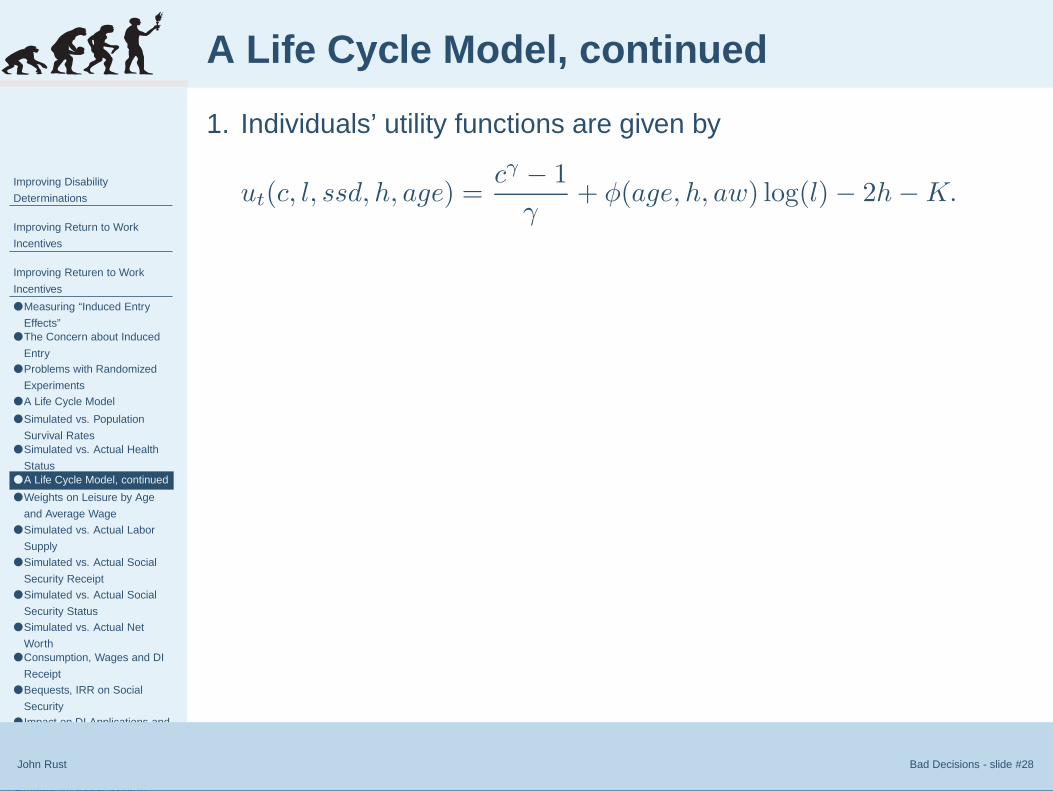
Improving Disability
Determinations
Improving Return to Work
Incentives
Improving Returen to Work
Incentives
● Measuring “Induced Entry
Effects”● The Concern about Induced
Entry● Problems with Randomized
Experiments
● A Life Cycle Model
● Simulated vs. Population
Survival Rates● Simulated vs. Actual Health
Status● A Life Cycle Model, continued
● Weights on Leisure by Age
and Average Wage
● Simulated vs. Actual Labor
Supply
● Simulated vs. Actual Social
Security Receipt
● Simulated vs. Actual Social
Security Status
● Simulated vs. Actual Net
Worth● Consumption, Wages and DI
Receipt
● Bequests, IRR on Social
Security● Impact on DI Applications and
Rolls● Impact on Labor Supply
● Impact on Wages and Taxes
● Impact on Social Security
● Impact on Wealth and
John Rust Bad Decisions - slide #28
A Life Cycle Model, continued
1. Individuals’ utility functions are given by
ut(c, l, ssd, h, age) =cγ − 1
γ+ φ(age, h, aw) log(l) − 2h − K.
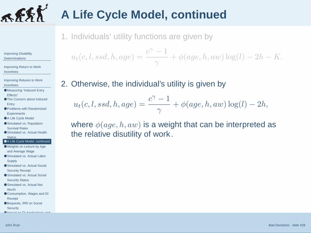
2. Otherwise, the individual’s utility is given by
ut(c, l, ssd, h, age) =cγ − 1
γ+ φ(age, h, aw) log(l) − 2h,
where φ(age, h, aw) is a weight that can be interpreted asthe relative disutility of work .
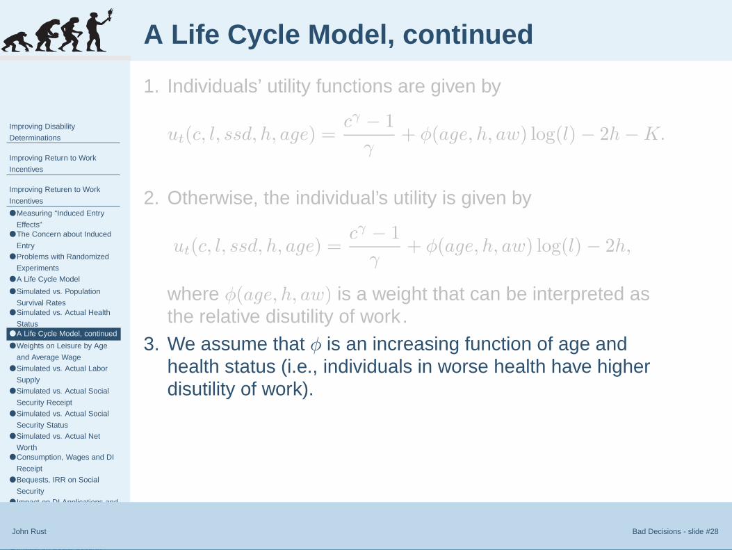
3. We assume that φ is an increasing function of age andhealth status (i.e., individuals in worse health have higherdisutility of work).
4. Wages at full time are given by the regression
log(yt+1) = α1 + α2 log(awt) + α3t + α4t2 + ηt.

John Rust Bad Decisions - slide #29
Weights on Leisure by Age and Average Wage
20 30 40 50 60 70 80 90 1000
2
4
6
8
10
12
Age
η(ag
e,h)
: wei
ght o
n le
isur
e in
util
ity fu
nctio
n
Relative weight on disutility of work as a functionof age and health status
DisabledPoor HealthGood Health
0 10 20 30 40 50 60 70 800
0.5
1
1.5
2
2.5Weight on disuility of work as a function of average wage
nuaw
(aw
): w
eigh
t on
utili
ty o
f lei
sure
Average Wages

John Rust Bad Decisions - slide #30
Simulated vs. Actual Labor Supply
45 50 55 60 65 700
0.1
0.2
0.3
0.4
0.5
0.6
0.7
0.8
Age
a. Actual Employment Status in the HRS
Fra
ctio
n of
sur
vivo
rs in
em
ploy
men
t sta
te
Full−timePart−timeNot working
45 50 55 60 65 700
0.1
0.2
0.3
0.4
0.5
0.6
0.7
0.8
0.9
Fra
ctio
n of
Sur
vivo
rs
Age
Simulated Employment Status
Full−timePart−timeNot working
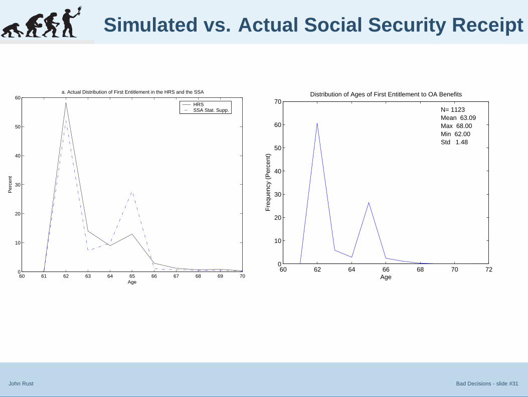
John Rust Bad Decisions - slide #31
Simulated vs. Actual Social Security Receipt
60 61 62 63 64 65 66 67 68 69 700
10
20
30
40
50
60
Age
a. Actual Distribution of First Entitlement in the HRS and the SSA
Per
cent
HRSSSA Stat. Supp.
60 62 64 66 68 70 720
10
20
30
40
50
60
70Distribution of Ages of First Entitlement to OA Benefits
N= 1123Mean 63.09Max 68.00Min 62.00Std 1.48
AgeF
requ
ency
(P
erce
nt)

John Rust Bad Decisions - slide #32
Simulated vs. Actual Social Security Status
46 48 50 52 54 56 58 60 62 64 66 680
0.1
0.2
0.3
0.4
0.5
0.6
0.7
0.8
0.9
1
Age
a. Actual Social Security Status in the HRS
Per
cent OA beneficiaries
DI beneficiariesNo SSA benefits
40 45 50 55 60 65 700
0.1
0.2
0.3
0.4
0.5
0.6
0.7
0.8
0.9
1
Fra
ctio
n of
Sur
vivo
rs
Age
Simulated Social Security Status
Not Eligible for SSOA BeneficiaryDI Beneficiary

John Rust Bad Decisions - slide #33
Simulated vs. Actual Net Worth
45 50 55 60 65 700
20
40
60
80
100
120
Age
a. Net Wealth and Earnings in the HRS
Med
ian
valu
e in
000
$ of
199
2, fo
r re
spon
dent
s
WealthHousing wealthStock wealthAfter tax earnings
20 30 40 50 60 70 80 90 100−20
0
20
40
60
80
100
120
140
160
180
Med
ian
Val
ue (
Dol
lars
) fo
r S
urvi
vors
in C
ohor
t
Age
Wealth, Wages, Consumption, and SS Benefits
WealthAfter Tax WagesConsumptionSS Benefits
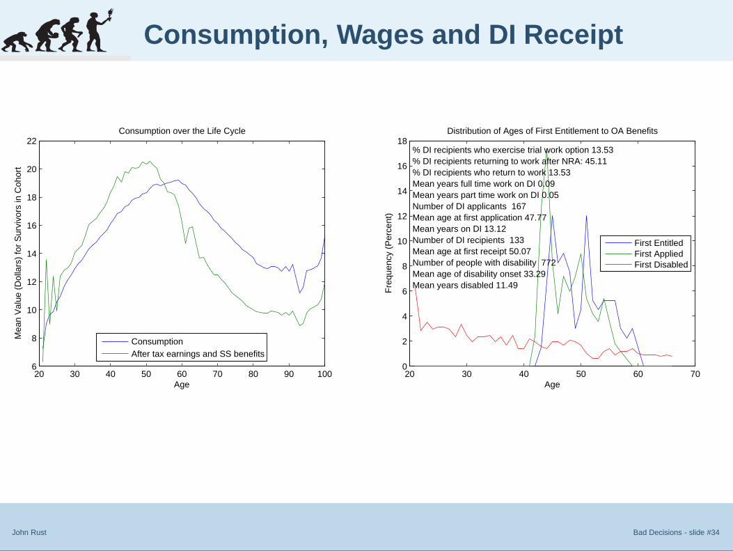
John Rust Bad Decisions - slide #34
Consumption, Wages and DI Receipt
20 30 40 50 60 70 80 90 1006
8
10
12
14
16
18
20
22Consumption over the Life Cycle
Age
Mea
n V
alue
(D
olla
rs)
for
Sur
vivo
rs in
Coh
ort
ConsumptionAfter tax earnings and SS benefits
20 30 40 50 60 700
2
4
6
8
10
12
14
16
18Distribution of Ages of First Entitlement to OA Benefits
AgeF
requ
ency
(P
erce
nt)
% DI recipients who exercise trial work option 13.53% DI recipients returning to work after NRA: 45.11% DI recipients who return to work 13.53Mean years full time work on DI 0.09Mean years part time work on DI 0.05Number of DI applicants 167Mean age at first application 47.77Mean years on DI 13.12Number of DI recipients 133Mean age at first receipt 50.07Number of people with disability 772Mean age of disability onset 33.29Mean years disabled 11.49
First EntitledFirst AppliedFirst Disabled
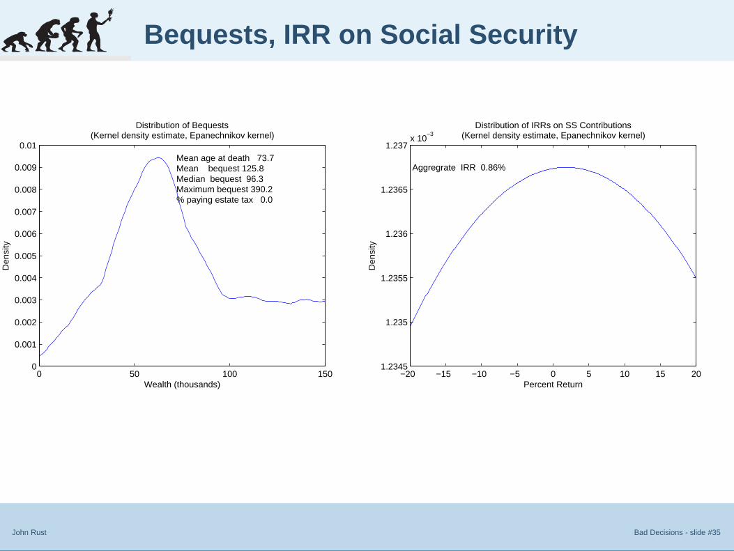
John Rust Bad Decisions - slide #35
Bequests, IRR on Social Security
0 50 100 1500
0.001
0.002
0.003
0.004
0.005
0.006
0.007
0.008
0.009
0.01
Distribution of Bequests(Kernel density estimate, Epanechnikov kernel)
Wealth (thousands)
Den
sity
Mean age at death 73.7Mean bequest 125.8Median bequest 96.3Maximum bequest 390.2% paying estate tax 0.0
−20 −15 −10 −5 0 5 10 15 201.2345
1.235
1.2355
1.236
1.2365
1.237x 10
−3Distribution of IRRs on SS Contributions
(Kernel density estimate, Epanechnikov kernel)
Percent Return
Den
sity
Aggregrate IRR 0.86%

John Rust Bad Decisions - slide #36
Impact on DI Applications and Rolls
40 45 50 55 60 650
2
4
6
8
10
12
14Impact of $1 for $2 Offset on SSDI Applications
Age
Per
cent
of P
opul
atio
n A
pply
ing
for
SS
DI
$1 for $2 OffsetStatus Quo
40 45 50 55 60 650
2
4
6
8
10
12
14Impact of $1 for $2 Offset on SSDI Roles
AgeP
erce
nt o
f Pop
ulat
ion
on S
SD
I
$1 for $2 OffsetStatus Quo

John Rust Bad Decisions - slide #37
Impact on Labor Supply
20 30 40 50 60 700
10
20
30
40
50
60
70
80Impact of $1 for $2 Offset on Full Time Work
Age
Per
cent
of S
SD
I Pop
ulat
ion
Wor
king
Ful
l Tim
e
$1 for $2 OffsetStatus Quo
20 30 40 50 60 700
5
10
15
20
25
30
35
40Impact of $1 for $2 Offset on Part Time Work
AgeP
erce
nt o
f SS
DI P
opul
atio
n W
orki
ng P
art T
ime
$1 for $2 OffsetStatus Quo
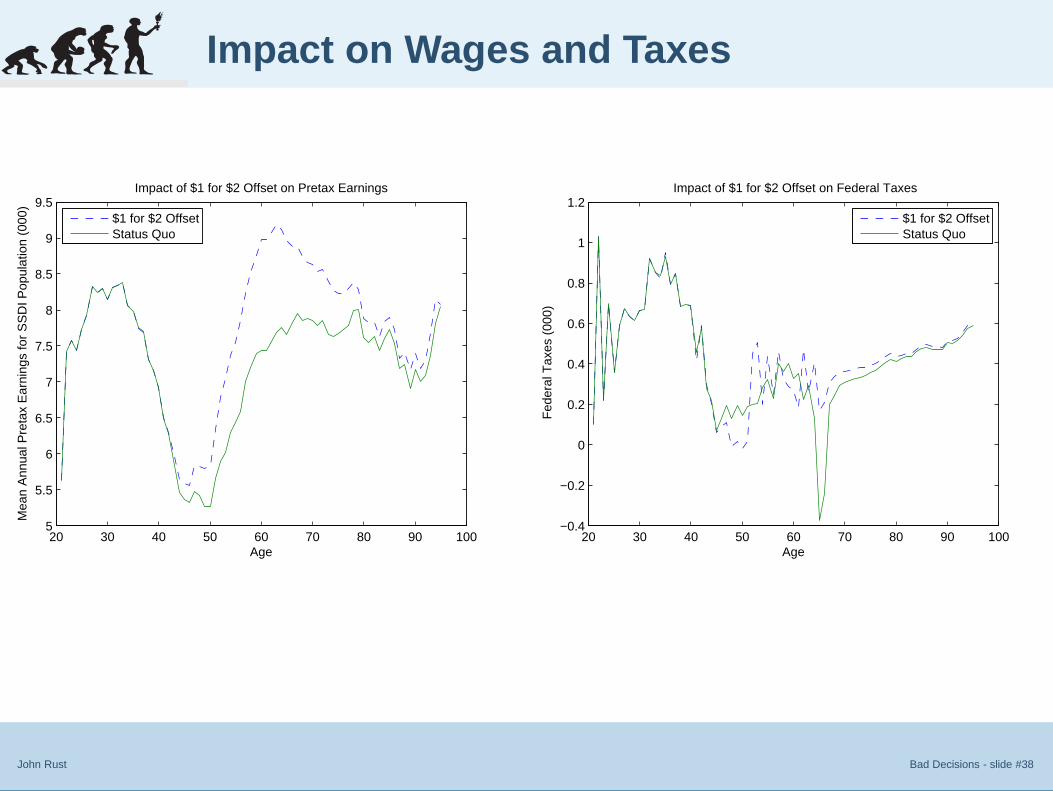
John Rust Bad Decisions - slide #38
Impact on Wages and Taxes
20 30 40 50 60 70 80 90 1005
5.5
6
6.5
7
7.5
8
8.5
9
9.5Impact of $1 for $2 Offset on Pretax Earnings
Age
Mea
n A
nnua
l Pre
tax
Ear
ning
s fo
r S
SD
I Pop
ulat
ion
(000
)
$1 for $2 OffsetStatus Quo
20 30 40 50 60 70 80 90 100−0.4
−0.2
0
0.2
0.4
0.6
0.8
1
1.2Impact of $1 for $2 Offset on Federal Taxes
AgeF
eder
al T
axes
(00
0)
$1 for $2 OffsetStatus Quo

John Rust Bad Decisions - slide #39
Impact on Social Security
20 30 40 50 60 70 80 90 1000
1
2
3
4
5
6
7
8
9Impact of $1 for $2 Offset on Social Security Benefits
Age
Soc
ial S
ecur
ity B
enef
its (
000)
$1 for $2 OffsetStatus Quo
20 30 40 50 60 70 80 90 1000
0.1
0.2
0.3
0.4
0.5
0.6
0.7
0.8Impact of $1 for $2 Offset on Social Security Contributions
AgeS
ocia
l Sec
urity
Con
trib
utio
ns (
000)
$1 for $2 OffsetStatus Quo

John Rust Bad Decisions - slide #40
Impact on Wealth and Consumption
20 30 40 50 60 70 80 90 10010
20
30
40
50
60
70
80
90
100Impact of $1 for $2 Offset on Net Worth
Age
Net
Wor
th fo
r S
SD
I Pop
ulat
ion
(000
)
$1 for $2 OffsetStatus Quo
20 30 40 50 60 70 80 90 1005
5.5
6
6.5
7
7.5
8
8.5
9
9.5Impact of $1 for $2 Offset on Consumption
AgeM
ean
Ann
ual C
onsu
mpt
ion
for
SS
DI P
opul
atio
n (0
00)
$1 for $2 OffsetStatus Quo

John Rust Bad Decisions - slide #41
Impact on Welfare
20 30 40 50 60 70 80 90 100−3
−2.5
−2
−1.5
−1
−0.5
0
0.5
1
1.5Impact of $1 for $2 Offset on Utility
Age
Cur
rent
Util
ity
$1 for $2 OffsetStatus Quo
20 30 40 50 60 70 80 90 100−10
0
10
20
30
40
50
60
70Impact of $1 for $2 Offset on Discounted Utility
AgeE
xpec
ted
Dis
coun
ted
Util
ity
$1 for $2 OffsetStatus Quo
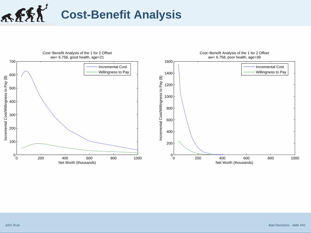
John Rust Bad Decisions - slide #42
Cost-Benefit Analysis
0 200 400 600 800 10000
100
200
300
400
500
600
700
Cost−Benefit Analysis of the 1 for 2 Offsetaw= 6.758, good health, age=21
Net Worth (thousands)
Incr
emen
tal C
ost/W
illin
gnes
s to
Pay
($)
Incremental CostWillingness to Pay
0 200 400 600 800 10000
200
400
600
800
1000
1200
1400
1600
Cost−Benefit Analysis of the 1 for 2 Offsetaw= 6.758, poor health, age=39
Net Worth (thousands)In
crem
enta
l Cos
t/Will
ingn
ess
to P
ay (
$)
Incremental CostWillingness to Pay

Improving Disability
Determinations
Improving Return to Work
Incentives
Improving Car Rental Profits
Improving Car Rental Profits
● What we did
● Conceptual Framework
● Econometric Methodology
● Main Findings
● Vehicle Aging Effects are ...
● hard to detect in young cars
● Implications for Replacement
● The Extrapolation Problem
● The “Pessimistic Scenario”
● Policy Recommendations
John Rust Bad Decisions - slide #44
What we did
1. We analyzed the vehicle replacement decisions by a rentalcar company.
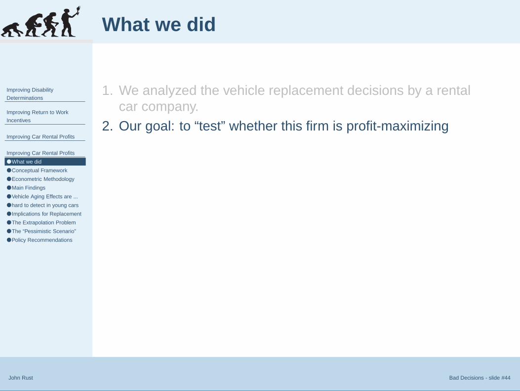
2. Our goal: to “test” whether this firm is profit-maximizing
Improving Disability
Determinations
Improving Return to Work
Incentives
Improving Car Rental Profits
Improving Car Rental Profits
● What we did
● Conceptual Framework
● Econometric Methodology
● Main Findings
● Vehicle Aging Effects are ...
● hard to detect in young cars
● Implications for Replacement
● The Extrapolation Problem
● The “Pessimistic Scenario”
● Policy Recommendations
John Rust Bad Decisions - slide #44
What we did
1. We analyzed the vehicle replacement decisions by a rentalcar company.
2. Our goal: to “test” whether this firm is profit-maximizing3. The firm is highly successful: its pre-tax IRR on car
investments ∼ 50%
4. Nevertheless, we present evidence that the firm is notmaximizing profits
5. We show that an alternative operating strategy can increaseprofits from 6 to 140%, depending on vehicle type
6. The alternative strategy: keep cars longer, and allowcustomers to choose new or old vehicles from a “menu” withdiscounts for older vehicles

Improving Disability
Determinations
Improving Return to Work
Incentives
Improving Car Rental Profits
Improving Car Rental Profits
● What we did
● Conceptual Framework
● Econometric Methodology
● Main Findings
● Vehicle Aging Effects are ...
● hard to detect in young cars
● Implications for Replacement
● The Extrapolation Problem
● The “Pessimistic Scenario”
● Policy Recommendations
John Rust Bad Decisions - slide #45
Conceptual Framework
1. We model the history of a rental car as a realization of asemi-Markov process.
2. A rental car can be in one of three possible states:

Improving Disability
Determinations
Improving Return to Work
Incentives
Improving Car Rental Profits
Improving Car Rental Profits
● What we did
● Conceptual Framework
● Econometric Methodology
● Main Findings
● Vehicle Aging Effects are ...
● hard to detect in young cars
● Implications for Replacement
● The Extrapolation Problem
● The “Pessimistic Scenario”
● Policy Recommendations
John Rust Bad Decisions - slide #45
Conceptual Framework
1. We model the history of a rental car as a realization of asemi-Markov process.
2. A rental car can be in one of three possible states:■ In a lot spell, waiting to be rented

Improving Disability
Determinations
Improving Return to Work
Incentives
Improving Car Rental Profits
Improving Car Rental Profits
● What we did
● Conceptual Framework
● Econometric Methodology
● Main Findings
● Vehicle Aging Effects are ...
● hard to detect in young cars
● Implications for Replacement
● The Extrapolation Problem
● The “Pessimistic Scenario”
● Policy Recommendations
John Rust Bad Decisions - slide #45
Conceptual Framework
1. We model the history of a rental car as a realization of asemi-Markov process.
2. A rental car can be in one of three possible states:■ In a lot spell, waiting to be rented■ In a short term rental spell

Improving Disability
Determinations
Improving Return to Work
Incentives
Improving Car Rental Profits
Improving Car Rental Profits
● What we did
● Conceptual Framework
● Econometric Methodology
● Main Findings
● Vehicle Aging Effects are ...
● hard to detect in young cars
● Implications for Replacement
● The Extrapolation Problem
● The “Pessimistic Scenario”
● Policy Recommendations
John Rust Bad Decisions - slide #45
Conceptual Framework
1. We model the history of a rental car as a realization of asemi-Markov process.
2. A rental car can be in one of three possible states:■ In a lot spell, waiting to be rented■ In a short term rental spell■ In a long term rental spell
3. We analyze three different types of vehicles in the companyfleet

Improving Disability
Determinations
Improving Return to Work
Incentives
Improving Car Rental Profits
Improving Car Rental Profits
● What we did
● Conceptual Framework
● Econometric Methodology
● Main Findings
● Vehicle Aging Effects are ...
● hard to detect in young cars
● Implications for Replacement
● The Extrapolation Problem
● The “Pessimistic Scenario”
● Policy Recommendations
John Rust Bad Decisions - slide #45
Conceptual Framework
1. We model the history of a rental car as a realization of asemi-Markov process.
2. A rental car can be in one of three possible states:■ In a lot spell, waiting to be rented■ In a short term rental spell■ In a long term rental spell
3. We analyze three different types of vehicles in the companyfleet■ A compact vehicle

Improving Disability
Determinations
Improving Return to Work
Incentives
Improving Car Rental Profits
Improving Car Rental Profits
● What we did
● Conceptual Framework
● Econometric Methodology
● Main Findings
● Vehicle Aging Effects are ...
● hard to detect in young cars
● Implications for Replacement
● The Extrapolation Problem
● The “Pessimistic Scenario”
● Policy Recommendations
John Rust Bad Decisions - slide #45
Conceptual Framework
1. We model the history of a rental car as a realization of asemi-Markov process.
2. A rental car can be in one of three possible states:■ In a lot spell, waiting to be rented■ In a short term rental spell■ In a long term rental spell
3. We analyze three different types of vehicles in the companyfleet■ A compact vehicle■ A luxury sedan

Improving Disability
Determinations
Improving Return to Work
Incentives
Improving Car Rental Profits
Improving Car Rental Profits
● What we did
● Conceptual Framework
● Econometric Methodology
● Main Findings
● Vehicle Aging Effects are ...
● hard to detect in young cars
● Implications for Replacement
● The Extrapolation Problem
● The “Pessimistic Scenario”
● Policy Recommendations
John Rust Bad Decisions - slide #45
Conceptual Framework
1. We model the history of a rental car as a realization of asemi-Markov process.
2. A rental car can be in one of three possible states:■ In a lot spell, waiting to be rented■ In a short term rental spell■ In a long term rental spell
3. We analyze three different types of vehicles in the companyfleet■ A compact vehicle■ A luxury sedan■ A recreational vehicle (RV)
4. Unfortunately, due to confidentiality restrictions on the data,we are not at liberty to disclose the name of the companyand cannot provide much more detail on the exactmakes/models of these cars or their locations.

Improving Disability
Determinations
Improving Return to Work
Incentives
Improving Car Rental Profits
Improving Car Rental Profits
● What we did
● Conceptual Framework
● Econometric Methodology
● Main Findings
● Vehicle Aging Effects are ...
● hard to detect in young cars
● Implications for Replacement
● The Extrapolation Problem
● The “Pessimistic Scenario”
● Policy Recommendations
John Rust Bad Decisions - slide #46
Econometric Methodology
1. We use econometric methods for duration and transitionmodels
2. We estimate hazard functions for spell durationsnon-parametrically
3. We estimate transitions between spells using a trinomiallogit model
4. We use regression analysis to predict resale prices ofvehicles
5. We use a parametric (Erlang) distribution to model vehicleusage (i.e. kilometers driven) during rental contracts.
6. We also model maintenance costs,
7. and estimate a binomial logit model of the firm’s sellingdecision
8. We then have all objects necessary to simulate the rentaloperations of this company

Improving Disability
Determinations
Improving Return to Work
Incentives
Improving Car Rental Profits
Improving Car Rental Profits
● What we did
● Conceptual Framework
● Econometric Methodology
● Main Findings
● Vehicle Aging Effects are ...
● hard to detect in young cars
● Implications for Replacement
● The Extrapolation Problem
● The “Pessimistic Scenario”
● Policy Recommendations
John Rust Bad Decisions - slide #47
Main Findings
1. We find that our simulation model provides a goodapproximation to the actual outcomes for this firm
2. In particular, our simulation model matches the high internalrates of return that this company earns under the statusquo.
3. However the value of having an econometric/simulationmodel is that we can evaluate the profitability of a widerange of alternative operating strategies
4. We formulate the optimal replacement problem and showthat it is equivalent to a regenerative optimal stoppingproblem.
5. We solve the stopping problem numerically and characterizecompare the optimal replacement policy to the firm’s currentreplacement policy.

Improving Disability
Determinations
Improving Return to Work
Incentives
Improving Car Rental Profits
Improving Car Rental Profits
● What we did
● Conceptual Framework
● Econometric Methodology
● Main Findings
● Vehicle Aging Effects are ...
● hard to detect in young cars
● Implications for Replacement
● The Extrapolation Problem
● The “Pessimistic Scenario”
● Policy Recommendations
John Rust Bad Decisions - slide #48
Vehicle Aging Effects are ...
1. We find that the predictions of the optimal stopping modelare sensitive to the specification of aging effects.
2. A key aging effect is the rapid depreciation in vehicle resalevalues.
3. However over the range of our observations, it is difficult todetect other significant aging effects.
4. In particular, rental rates, maintenance costs, and durationsof lot spells and rental spells show no evidence of agingeffects
5. The only aging effect that we can detect is a rental contractcomposition effect.
Improving Disability
Determinations
Improving Return to Work
Incentives
Improving Car Rental Profits
Improving Car Rental Profits
● What we did
● Conceptual Framework
● Econometric Methodology
● Main Findings
● Vehicle Aging Effects are ...
● hard to detect in young cars
● Implications for Replacement
● The Extrapolation Problem
● The “Pessimistic Scenario”
● Policy Recommendations
John Rust Bad Decisions - slide #49
hard to detect in young cars
1. That is, new cars tend to start off in long term rentalcontracts, but as they age, there is an increasing chance thecontracts will switch from long term to short term.
2. Durations on the lot tend to be longer between short termrentals since long term rentals have a high chance ofrollover.
3. Thus, the fraction of time spent on the lot tends to increaseas a vehicle ages (i.e. as its odometer increases).
4. It is difficult to detect aging effects for very old cars, becausefew such cars can be observed under the status quo.
5. The average age at sale is about 3 years, and the meanodometer at time of sale is about 70,000 kilometers.
6. We observe only a very few cars that are over 5 years old orwhose odometers have more than 140,000 kilometers.

Improving Disability
Determinations
Improving Return to Work
Incentives
Improving Car Rental Profits
Improving Car Rental Profits
● What we did
● Conceptual Framework
● Econometric Methodology
● Main Findings
● Vehicle Aging Effects are ...
● hard to detect in young cars
● Implications for Replacement
● The Extrapolation Problem
● The “Pessimistic Scenario”
● Policy Recommendations
John Rust Bad Decisions - slide #50
Implications for Replacement
1. If the only aging effects are resale price depreciation andthe gradual switch from long term to short term contracts,
2. the optimal policy is to never sell the car!
3. Intuition for result:

Improving Disability
Determinations
Improving Return to Work
Incentives
Improving Car Rental Profits
Improving Car Rental Profits
● What we did
● Conceptual Framework
● Econometric Methodology
● Main Findings
● Vehicle Aging Effects are ...
● hard to detect in young cars
● Implications for Replacement
● The Extrapolation Problem
● The “Pessimistic Scenario”
● Policy Recommendations
John Rust Bad Decisions - slide #50
Implications for Replacement
1. If the only aging effects are resale price depreciation andthe gradual switch from long term to short term contracts,
2. the optimal policy is to never sell the car!
3. Intuition for result:■ replacement of cars is a costly “investment” precisely due
to the rapid price depreciation.

Improving Disability
Determinations
Improving Return to Work
Incentives
Improving Car Rental Profits
Improving Car Rental Profits
● What we did
● Conceptual Framework
● Econometric Methodology
● Main Findings
● Vehicle Aging Effects are ...
● hard to detect in young cars
● Implications for Replacement
● The Extrapolation Problem
● The “Pessimistic Scenario”
● Policy Recommendations
John Rust Bad Decisions - slide #50
Implications for Replacement
1. If the only aging effects are resale price depreciation andthe gradual switch from long term to short term contracts,
2. the optimal policy is to never sell the car!
3. Intuition for result:■ replacement of cars is a costly “investment” precisely due
to the rapid price depreciation.■ if rental rates and maintenance costs do not decline with
age/odometer, then it is optimal to “amortize” the initialinvestment in a vehicle by keeping and maintaining itindefinitely.
4. Of course, it is unreasonable to suppose that rental rateswould not decrease if the company kept its vehicle stockindefinitely
5. Customers prefer new cars, all other things equal!

Improving Disability
Determinations
Improving Return to Work
Incentives
Improving Car Rental Profits
Improving Car Rental Profits
● What we did
● Conceptual Framework
● Econometric Methodology
● Main Findings
● Vehicle Aging Effects are ...
● hard to detect in young cars
● Implications for Replacement
● The Extrapolation Problem
● The “Pessimistic Scenario”
● Policy Recommendations
John Rust Bad Decisions - slide #51
The Extrapolation Problem
1. Thus, we face an extrapolation problem: we do not observethe company keeping cars very long in the data.
2. Lacking data on maintenance costs and rental histories forvery old cars, it is hazardous to make out of sample policypredictions about what will have if the company keeps carsfar longer than it currently does.
3. Our approach: make pessimistic assumptions aboutincreases in maintenance costs and required discounts onolder cars.
4. Assume that beyond 130,000 kilometers average dailymaintenance costs increase rapidly, increasing by a factor of11 by the time the odometer reaches 400,000 kilometers.
5. We also assume that with appropriate odometer-baseddiscounts on rental vehicles, customers can be induced torent older vehicles.

Improving Disability
Determinations
Improving Return to Work
Incentives
Improving Car Rental Profits
Improving Car Rental Profits
● What we did
● Conceptual Framework
● Econometric Methodology
● Main Findings
● Vehicle Aging Effects are ...
● hard to detect in young cars
● Implications for Replacement
● The Extrapolation Problem
● The “Pessimistic Scenario”
● Policy Recommendations
John Rust Bad Decisions - slide #52
The “Pessimistic Scenario”
1. Assume that daily rental rates are flat until 130,000kilometers, but decrease linearly with odometer thereafter,until rates hit 0 at 400,000 kilometers.
2. Even under these unrealistically pessimistic assumptions,we find that it is still optimal to keep vehicles roughly twiceas long as the company currently keeps them.
3. The optimal replacement threshold in the pessimisticscenario is 150,000 kilometers, about twice as large asunder the status quo.
4. Expected discounted profits increase significantly.Depending on the type of car, we predict profits will bebetween 18-240 percent larger than the status quo if itadopts the optimal replacement policy.

Improving Disability
Determinations
Improving Return to Work
Incentives
Improving Car Rental Profits
Improving Car Rental Profits
● What we did
● Conceptual Framework
● Econometric Methodology
● Main Findings
● Vehicle Aging Effects are ...
● hard to detect in young cars
● Implications for Replacement
● The Extrapolation Problem
● The “Pessimistic Scenario”
● Policy Recommendations
John Rust Bad Decisions - slide #53
Policy Recommendations
1. We recommend that the company undertake an experimentwith cars assigned to the treatment group kept longer andrental rates are discounted after a certain age/odometerthreshold.
2. The treatment effect is the increase in profit/internal rate ofreturn in the treatment group relative to the control group(i.e. the status quo operating policy.
3. Drawback of experiments: they are costly and timeconsuming, and may contaminate customers who receivediscounts, leading them to expect similar discounts at otherlocations.
4. In the absence of experimental data, we believemodel-based predictions such as ours, can be usefuldevices to help a company evaluate the profitability of itscurrent operating strategy.


Improving Disability
Determinations
Improving Return to Work
Incentives
Improving Car Rental Profits
2.1 Analyzing Rentals
● Rental Contracts
● Typical Rental Histories
● Comments
John Rust Bad Decisions - slide #55
Rental Contracts
1. The firm rents its cars on two types of contracts

Improving Disability
Determinations
Improving Return to Work
Incentives
Improving Car Rental Profits
2.1 Analyzing Rentals
● Rental Contracts
● Typical Rental Histories
● Comments
John Rust Bad Decisions - slide #55
Rental Contracts
1. The firm rents its cars on two types of contracts■ long term contracts with typical durations of 30 days,

Improving Disability
Determinations
Improving Return to Work
Incentives
Improving Car Rental Profits
2.1 Analyzing Rentals
● Rental Contracts
● Typical Rental Histories
● Comments
John Rust Bad Decisions - slide #55
Rental Contracts
1. The firm rents its cars on two types of contracts■ long term contracts with typical durations of 30 days,■ short term contract with typical durations of 3-4 days.
2. Customers are allowed to roll over a 30 day long termcontract into a defacto equivalent of a long term lease.
3. There is a penalty for early returns of vehicles in long termcontracts, generally equal to 20% of the lost rental revenuefor the unfinished remaining days in the contract.

John Rust Bad Decisions - slide #56
Typical Rental Histories
100 200 300 400 500 600 700 800 900 10000
1
2Rental History for Compact, urban location (service life: 1115 days, IRR=78.6%)
Day in Life of Car
Rent
al St
ate
100 200 300 400 500 600 700 800 9000
1
2Rental History for Luxury 1, urban location (service life: 995 days, IRR=57.6%)
Day in Life of Car
Rent
al St
ate
100 200 300 400 500 6000
1
2Rental History for RV, tourist location (service life: 810 days, IRR=96.6%)
Day in Life of Car
Rent
al St
ate

Improving Disability
Determinations
Improving Return to Work
Incentives
Improving Car Rental Profits
2.1 Analyzing Rentals
● Rental Contracts
● Typical Rental Histories
● Comments
John Rust Bad Decisions - slide #57
Comments
1. Recall, the IRR is the r that solves
0 =T∑
t=0
exp{−atr/365}ct,(1)
where ct is the cash inflow (if positive) or outflow (ifnegative), and at is the number of days after the initial
purchase of the vehicle that the tth cash flow occurred.

Improving Disability
Determinations
Improving Return to Work
Incentives
Improving Car Rental Profits
2.1 Analyzing Rentals
● Rental Contracts
● Typical Rental Histories
● Comments
John Rust Bad Decisions - slide #57
Comments
1. Recall, the IRR is the r that solves
0 =T∑
t=0
exp{−atr/365}ct,(1)
where ct is the cash inflow (if positive) or outflow (ifnegative), and at is the number of days after the initial
purchase of the vehicle that the tth cash flow occurred.2. Thus, c0 < 0 and a0 = 0 represent the initial purchase of the
car, aT is the service life and cT is the resale price thecompany receives from selling the car in the used carmarket, or at an auction.
3. We see that for each of the cars illustrated in figure 1, therealized rates of return are extraordinarily high. These highreturns are not atypical.

John Rust Bad Decisions - slide #59
Return distribution: Compact
−0.2 0 0.2 0.4 0.6 0.8 1 1.2 1.4 1.6 1.80
0.2
0.4
0.6
0.8
1
Distribution of Internal Rates of Return on Compact, all locations
Den
sity
Internal Rates of Return on Compact, all locations
Mean 0.76776Median 0.65936Minimum −0.017Maximum 9.2275Std dev 0.72254Observations 167
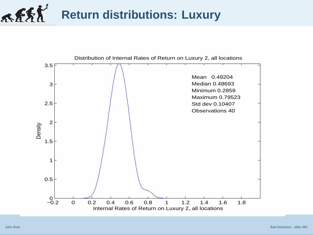
John Rust Bad Decisions - slide #60
Return distributions: Luxury
−0.2 0 0.2 0.4 0.6 0.8 1 1.2 1.4 1.6 1.80
0.5
1
1.5
2
2.5
3
3.5
Distribution of Internal Rates of Return on Luxury 2, all locations
Den
sity
Internal Rates of Return on Luxury 2, all locations
Mean 0.49204Median 0.48693Minimum 0.2859Maximum 0.79523Std dev 0.10407Observations 40
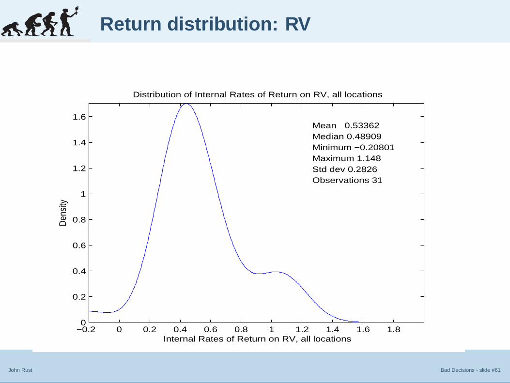
John Rust Bad Decisions - slide #61
Return distribution: RV
−0.2 0 0.2 0.4 0.6 0.8 1 1.2 1.4 1.6 1.80
0.2
0.4
0.6
0.8
1
1.2
1.4
1.6
Distribution of Internal Rates of Return on RV, all locations
Den
sity
Internal Rates of Return on RV, all locations
Mean 0.53362Median 0.48909Minimum −0.20801Maximum 1.148Std dev 0.2826Observations 31

Improving Disability
Determinations
Improving Return to Work
Incentives
Improving Car Rental Profits
2.2 Analyzing Returns
● Return distribution: Compact
● Return distributions: Luxury
● Return distribution: RV
● Analysis of returns
● Regression results: IRR
● Discussion of results
● Why no age/odometer effect?
John Rust Bad Decisions - slide #62
Analysis of returns
1. Which factors affect/determine the return on a rental car?
■ Rental rates
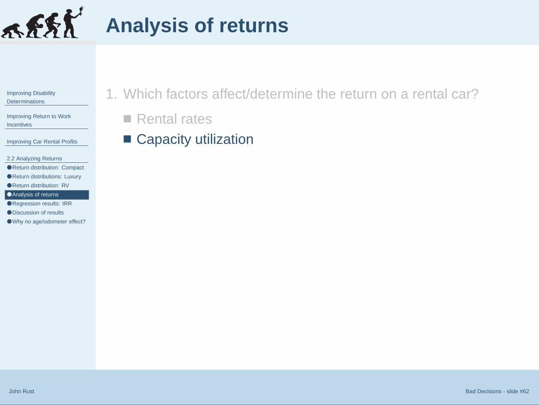
Improving Disability
Determinations
Improving Return to Work
Incentives
Improving Car Rental Profits
2.2 Analyzing Returns
● Return distribution: Compact
● Return distributions: Luxury
● Return distribution: RV
● Analysis of returns
● Regression results: IRR
● Discussion of results
● Why no age/odometer effect?
John Rust Bad Decisions - slide #62
Analysis of returns
1. Which factors affect/determine the return on a rental car?
■ Rental rates■ Capacity utilization

Improving Disability
Determinations
Improving Return to Work
Incentives
Improving Car Rental Profits
2.2 Analyzing Returns
● Return distribution: Compact
● Return distributions: Luxury
● Return distribution: RV
● Analysis of returns
● Regression results: IRR
● Discussion of results
● Why no age/odometer effect?
John Rust Bad Decisions - slide #62
Analysis of returns
1. Which factors affect/determine the return on a rental car?
■ Rental rates■ Capacity utilization■ New purchase price and resale value

Improving Disability
Determinations
Improving Return to Work
Incentives
Improving Car Rental Profits
2.2 Analyzing Returns
● Return distribution: Compact
● Return distributions: Luxury
● Return distribution: RV
● Analysis of returns
● Regression results: IRR
● Discussion of results
● Why no age/odometer effect?
John Rust Bad Decisions - slide #62
Analysis of returns
1. Which factors affect/determine the return on a rental car?
■ Rental rates■ Capacity utilization■ New purchase price and resale value■ service life of vehicle
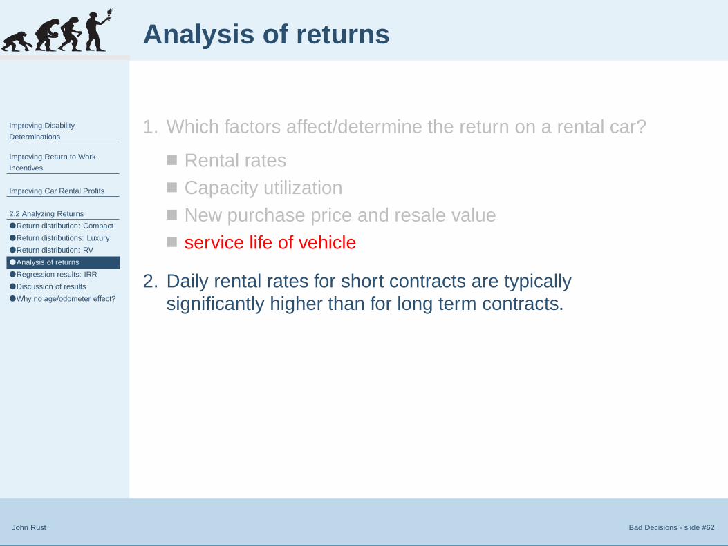
2. Daily rental rates for short contracts are typicallysignificantly higher than for long term contracts.
3. Counterbalancing this, is that cars are more likely to be onthe lot between successive short term rental spells.
4. Which contract is more profitable: long or short term?

John Rust Bad Decisions - slide #63
Regression results: IRR
Variable Compact Luxury RV
Constant 0.575∗ −0.006 0.999
Utilization Rate 0.003 0.522∗ 1.366∗
Fraction Rented Long Term −0.220∗ −0.076 −0.876∗
Total Maintenance costs ($000) −7.46e−5∗ −2.00e−5 6.978e−6
Odometer (000 km) 0.0007 −0.0004 −0.001
Age at Sale (years) 0.151∗ 0.072 −0.154
New Price ($000) −0.104∗ −0.036∗ −0.082∗
Sale Price ($000) 0.008 −0.002 0.063
Short term rental rate 0.003∗ 0.0006∗ 0.004∗
Long term rental rate 0.037∗∗ 0.020∗∗ 0.009
Observations,R2 167,81% 40,78% 31,86%
Improving Disability
Determinations
Improving Return to Work
Incentives
Improving Car Rental Profits
2.2 Analyzing Returns
● Return distribution: Compact
● Return distributions: Luxury
● Return distribution: RV
● Analysis of returns
● Regression results: IRR
● Discussion of results
● Why no age/odometer effect?
John Rust Bad Decisions - slide #64
Discussion of results
1. Regression results generally confirm our expectations:
■ higher purchase prices reduce the IRR, resale pricesincrease it
■ the estimate of utilization rate is positive and statisticallysignificant
■ the daily rental rates are also positive and generallysignificant.
■ the fraction of the time the car was rented long term has anegative coefficient, suggesting long term contracts areless profitable than short term contracts
2. However estimates of maintenance costs ambiguous,
3. and coefficients on age and odometer are insignificantlydifferent from 0.
Improving Disability
Determinations
Improving Return to Work
Incentives
Improving Car Rental Profits
2.2 Analyzing Returns
● Return distribution: Compact
● Return distributions: Luxury
● Return distribution: RV
● Analysis of returns
● Regression results: IRR
● Discussion of results
● Why no age/odometer effect?
John Rust Bad Decisions - slide #65
Why no age/odometer effect?
1. There are several possible reasons why effect of age,odometer, and maintenance costs are insignificantlydifferent from 0.
2. One reason is multicollinearity especially between age andodometer.
3. However if the regression and includes only age orodometer individually, the results are still generallyinsignificant.
4. Only in one case, for the luxury vehicle, are both age andmaintenance significant
5. In the luxury case, age has a positive coefficient and totalmaintenance cost has a negative coefficient.
6. But even in this case, the effect of age on IRR is small: theregression results predict that keeping a luxury car for 100more days increases the IRR by 0.03.
Improving Disability
Determinations
Improving Return to Work
Incentives
Improving Car Rental Profits
2.3 Is regression enough?
● A sign of optimality?
● Results for simulated optimal
replacements
● Can we find an Instrument?
● How to proceed?
John Rust Bad Decisions - slide #67
A sign of optimality?
1. Let Π(o) denote the expected discounted profits from sellinga car at odometer value o
2. If the firm chooses an optimal threshold o∗, then
∂Π
∂o(o∗) = 0.(2)
so small variations in o should not affect profits and IRR.
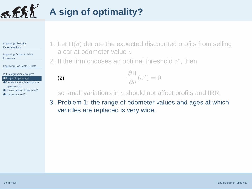
Improving Disability
Determinations
Improving Return to Work
Incentives
Improving Car Rental Profits
2.3 Is regression enough?
● A sign of optimality?
● Results for simulated optimal
replacements
● Can we find an Instrument?
● How to proceed?
John Rust Bad Decisions - slide #67
A sign of optimality?
1. Let Π(o) denote the expected discounted profits from sellinga car at odometer value o
2. If the firm chooses an optimal threshold o∗, then
∂Π
∂o(o∗) = 0.(2)
so small variations in o should not affect profits and IRR.3. Problem 1: the range of odometer values and ages at which
vehicles are replaced is very wide.
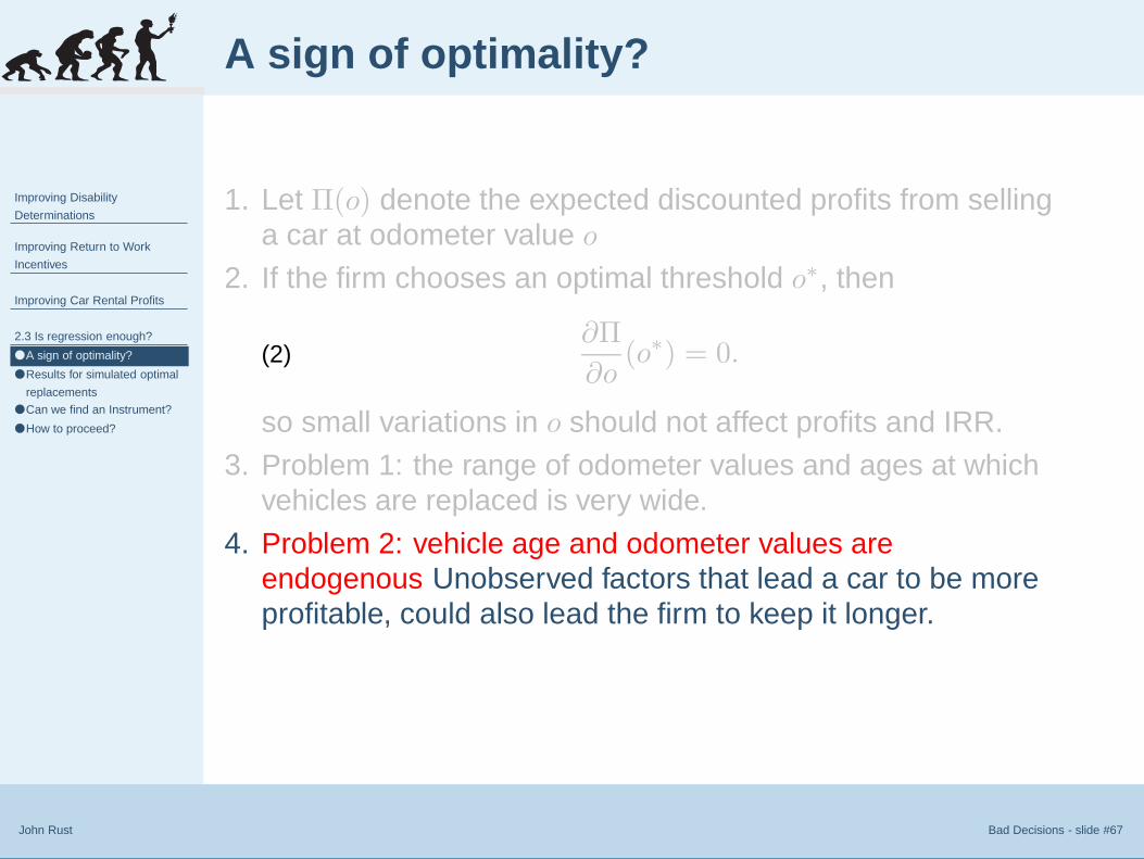
4. Problem 2: vehicle age and odometer values areendogenous Unobserved factors that lead a car to be moreprofitable, could also lead the firm to keep it longer.
5. If so, we would expect a positive correlation between vehicleage and odometer values and the error term in theregression, so the estimates for these coefficients could beupward biased.

John Rust Bad Decisions - slide #68
Results for simulated optimal replacements
Variable Compact Luxury RV
Constant 0.875∗ 0.619 −0.261
Utilization Rate 0.750∗ 0.399∗ 0.791∗
Fraction Rented Long Term −0.535∗ −0.142∗ −0.597∗
Odometer (000 km) 0.002 −0.0003 0.002∗
Age at Sale (years) 0.122∗ −0.002 −0.040
Sale Price ($000) 0.009 0.002 0.003
Short term rental rate 0.0006 0.0003 0.003
Long term rental rate 0.008 −0.005 0.008
Observations,R2 100,67% 100,56% 100,56%

Improving Disability
Determinations
Improving Return to Work
Incentives
Improving Car Rental Profits
2.3 Is regression enough?
● A sign of optimality?
● Results for simulated optimal
replacements
● Can we find an Instrument?
● How to proceed?
John Rust Bad Decisions - slide #69
Can we find an Instrument?
1. What we need is an instrumental variable that causesexogenous shifts in the age at which the company replacedsome of its vehicles.
2. An example of such a variable might be a recall dummy.
3. That is, if there was some major problem in one of the typesof cars that the company owned that resulted in massrecalls or prompted the company to sell the cars“prematurely” this might constitute a valid instrument.
4. However a better “instrument” is a treatment dummy.
5. That is, if the company had undertaken a randomizedexperiment, keeping some cars longer than it would haveotherwise.
6. Unfortunately, we do not have either of these instrumentalvariables in our data set.

Improving Disability
Determinations
Improving Return to Work
Incentives
Improving Car Rental Profits
2.3 Is regression enough?
● A sign of optimality?
● Results for simulated optimal
replacements
● Can we find an Instrument?
● How to proceed?
John Rust Bad Decisions - slide #70
How to proceed?
1. In the absence of any good instruments, and if the companyhas not undertaken any experiments, how can we proceedto test the hypothesis, i.e. is the company maximizingprofits?
2. Our approach: to create a model of the firm’s rentaloperations.
3. We estimate the unknown parameters of this model usingthe company’s data.
4. Once the model is estimated, we can simulate it.
5. We will simulate the model under the status quo and show itprovides a good approximation to the data we observe.
6. Then we use the model to compute and simulate alternativerental policies. We show that certain alternative policiesresult in significantly higher profits.


Improving Disability
Determinations
Improving Return to Work
Incentives
Improving Car Rental Profits
3.1 Overview
● A Semi-Markov Model
● Other State Variables
● Implied State Variables
● Model Components
John Rust Bad Decisions - slide #72
A Semi-Markov Model
■ In this model, a car can be in one of four possible states atany given point in time:
1. In a long term rental contract (i.e. a “long term rentalspell”),
2. In a short term rental contract (i.e. a “short term rentalspell”),
3. In the lot waiting to be rented, where the previous rentalstate was a long term rental spell,
4. In the lot waiting to be rented, where the previous rentalstate was a short term rental spell.
■ We refer to the latter two states, 3 and 4, as lot spells.

Improving Disability
Determinations
Improving Return to Work
Incentives
Improving Car Rental Profits
3.1 Overview
● A Semi-Markov Model
● Other State Variables
● Implied State Variables
● Model Components
John Rust Bad Decisions - slide #73
Other State Variables
■ in addition to the rental state rt ∈ {1, 2, 3, 4} other relevantstate variables for modeling the decisions of the rentalcompany are:
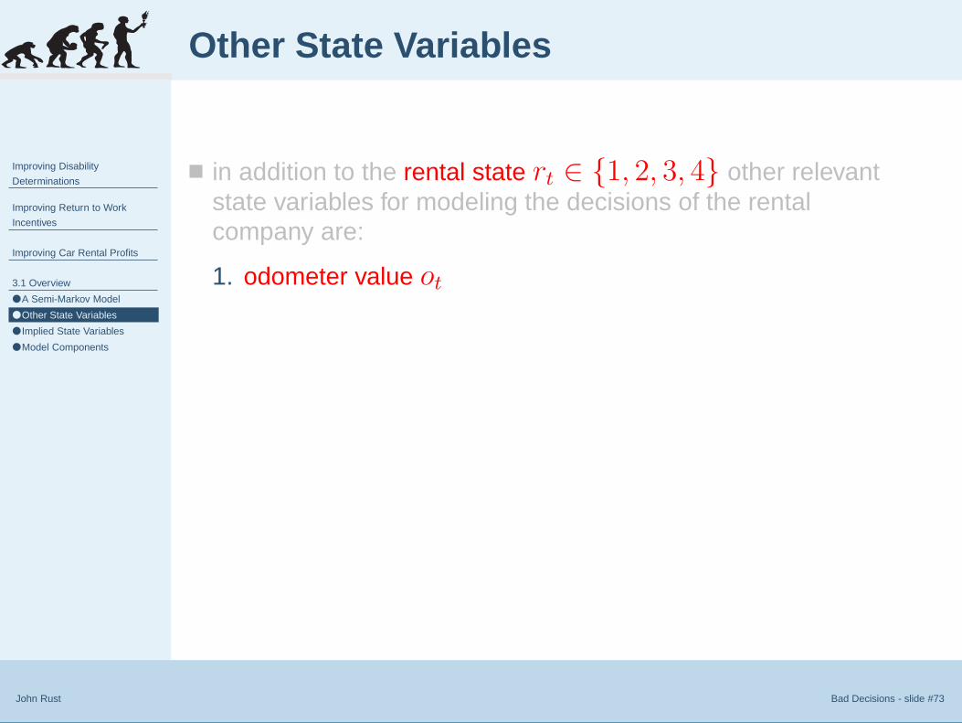
1. odometer value ot
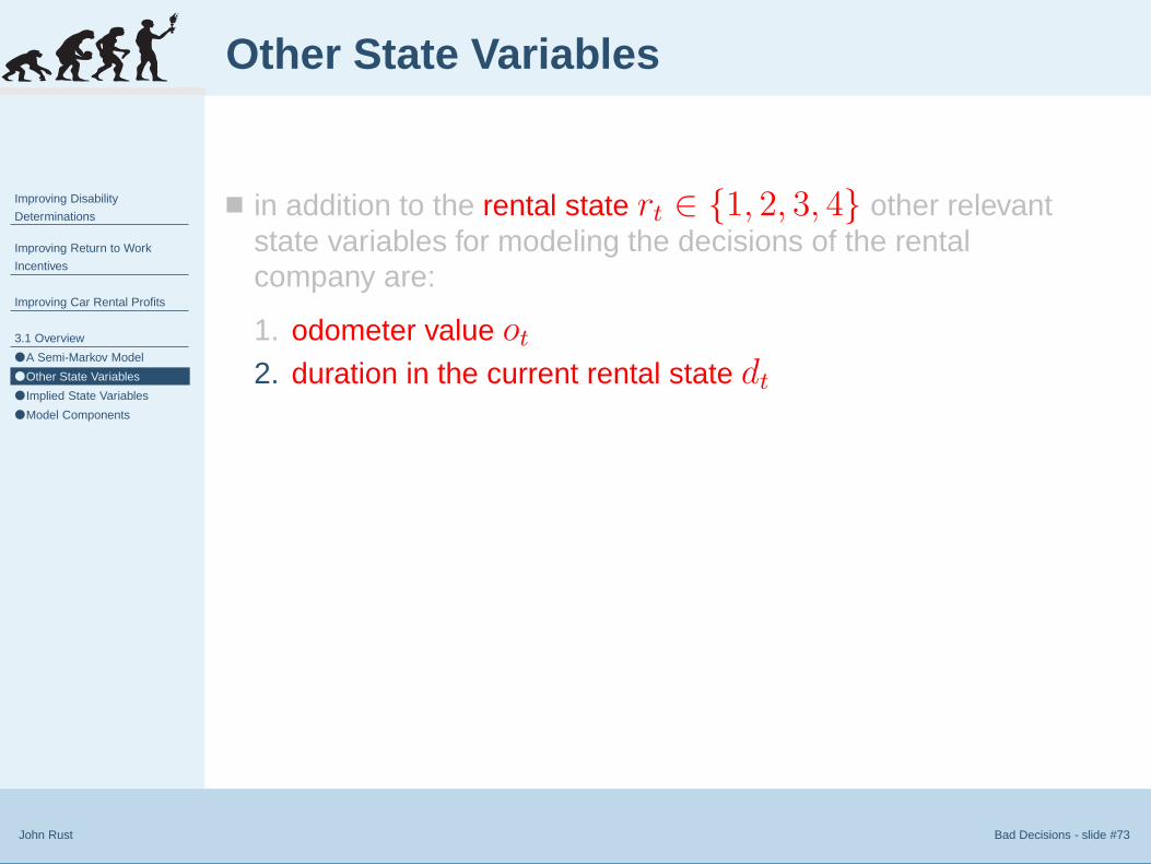
2. duration in the current rental state dt
■ Thus, we seek to model the joint stochastic process{rt, ot, dt}.
■ The other potential state variable of interest, the vehicle’sage at creates complications due to non-stationarity.
■ Since age and odometer are highly correlated, we feel thatnot much damage is done from excluding at as an explicitstate variable, and deriving the implied distribution of vehicleages from our model.

Improving Disability
Determinations
Improving Return to Work
Incentives
Improving Car Rental Profits
3.1 Overview
● A Semi-Markov Model
● Other State Variables
● Implied State Variables
● Model Components
John Rust Bad Decisions - slide #74
Implied State Variables
■ Once we estimate the stochastic process {rt, ot, dt}, we canderive/simulate other variables of interest, including

Improving Disability
Determinations
Improving Return to Work
Incentives
Improving Car Rental Profits
3.1 Overview
● A Semi-Markov Model
● Other State Variables
● Implied State Variables
● Model Components
John Rust Bad Decisions - slide #74
Implied State Variables
■ Once we estimate the stochastic process {rt, ot, dt}, we canderive/simulate other variables of interest, including1. rental revenues
2. maintenance costs
3. rental profits and internal rates of return

Improving Disability
Determinations
Improving Return to Work
Incentives
Improving Car Rental Profits
3.1 Overview
● A Semi-Markov Model
● Other State Variables
● Implied State Variables
● Model Components
John Rust Bad Decisions - slide #74
Implied State Variables
■ Once we estimate the stochastic process {rt, ot, dt}, we canderive/simulate other variables of interest, including1. rental revenues
2. maintenance costs
3. rental profits and internal rates of return■ However to do this, we also need econometric models for a
vehicle’s resale price and a model of the the timing of thereplacement decision.
■ With this information, we can construct a completeeconometric model of the company’s rental operations, andconduct stochastic simulations of the model to see howaccurately it can represent the company’s actual operations.

Improving Disability
Determinations
Improving Return to Work
Incentives
Improving Car Rental Profits
3.1 Overview
● A Semi-Markov Model
● Other State Variables
● Implied State Variables
● Model Components
John Rust Bad Decisions - slide #75
Model Components
1. A model of resale prices

Improving Disability
Determinations
Improving Return to Work
Incentives
Improving Car Rental Profits
3.1 Overview
● A Semi-Markov Model
● Other State Variables
● Implied State Variables
● Model Components
John Rust Bad Decisions - slide #75
Model Components
1. A model of resale prices
2. A duration model for the random durations of a car in eachof the rental and lot states,
3. A transition model a a vehicle’s transitions between rentalstates at the end of the current rental spell
4. A utilization model for the kilometers driven during a long orshort term rental contract,
5. A model for maintenance costs incurred by the companyover the life of the car,
6. A model of the company’s replacement decision, i.e. thefactors that motivate it to sell a given car at a particular pointin time.


Improving Disability
Determinations
Improving Return to Work
Incentives
Improving Car Rental Profits
3.2 Resale Price Model
● The resale price model
● Resale price regression
● Resale prices: Compact
● Resale prices: Luxury
● Resale prices: RV
● Comments
● Conclusions: resale prices
John Rust Bad Decisions - slide #77
The resale price model
■ We have data on both the new price P (τ) as well as therealized sales price Pt(ot, τ) of each car, where τ denotes aparticular make and model of vehicle, which we will also calla car type.
■ For each of the three car types τ ∈ {compact, luxury, RV},we estimated a simple linear regression model with the logdepreciation rate, P (τ)/Pt(ot, τ), as the dependent variable
log(P (τ)/Pt(ot, τ)) = α1(τ) + α2(τ)ot + εt.(3)
■ The type-specific “depreciation coefficients” (α1(τ), α2(τ))are used to predict resale prices.
■ We also estimated regressions that included vehicle age andother variables such as the number of accidents and the totalaccident repair cost.

John Rust Bad Decisions - slide #78
Resale price regression
Variable Compact Luxury RV
Constant −0.4789∗ −0.6201∗∗ −0.8521∗
Age (days) −0.0001∗ −0.0004∗ −0.0004∗
Odometer (000 km) −0.0007∗ −0.0011∗ 0.0016
Number of Accidents −0.0112 0.0006 0.0371
Accident Repair Costs −0.8.88e−6 −4.672e−6 −1.654e−6
Internal Rate of Return 0.1629∗∗ 0.067 0.394∗
Maintenance Cost per Day 0.0092 −0.0039 −0.0053
N , R2 288,38.9% 91,42.0% 41,48.1%

John Rust Bad Decisions - slide #79
Resale prices: Compact
0 50 100 150 200 250 300 350 4003500
4000
4500
5000
5500
6000
6500
7000
7500
8000
8500
Odometer (thousands of kilometers
Res
ale
pric
e of
car
(th
ousa
nds
of d
olla
rs)
Predicted versus Actual Resale Prices for Compact, all locations
Mean Price New 9669Mean Sale Price 5478Max Sale Price 7290Min Sale Price 3500Mean Odometer at Sale 77914Max Odometer at Sale 153143Min Odometer at Sale 10500Number of Observations 288

John Rust Bad Decisions - slide #80
Resale prices: Luxury
0 50 100 150 200 250 300 350 400
0.8
1
1.2
1.4
1.6
1.8
2
x 104
Odometer (thousands of kilometers
Res
ale
pric
e of
car
(th
ousa
nds
of d
olla
rs)
Predicted versus Actual Resale Prices for Luxury 2, all locations
Mean Price New 23389Mean Sale Price 12014Max Sale Price 16550Min Sale Price 7500Mean Odometer at Sale 74684Max Odometer at Sale 187800Min Odometer at Sale 35000Number of Observations 91

John Rust Bad Decisions - slide #81
Resale prices: RV
0 50 100 150 200 250 300 350 4000.4
0.6
0.8
1
1.2
1.4
1.6
x 104
Odometer (thousands of kilometers
Res
ale
pric
e of
car
(th
ousa
nds
of d
olla
rs)
Predicted versus Actual Resale Prices for RV, all locations
Mean Price New 18774Mean Sale Price 7751Max Sale Price 10550Min Sale Price 4000Mean Odometer at Sale 88829Max Odometer at Sale 163860Min Odometer at Sale 38000Number of Observations 41

Improving Disability
Determinations
Improving Return to Work
Incentives
Improving Car Rental Profits
3.2 Resale Price Model
● The resale price model
● Resale price regression
● Resale prices: Compact
● Resale prices: Luxury
● Resale prices: RV
● Comments
● Conclusions: resale prices
John Rust Bad Decisions - slide #82
Comments
1. The constant term in the regressions measures the theinstantaneous depreciation in car prices the minute it leavesthe new car lot.
2. We see that the instantaneous depreciation is huge for allthree vehicle types: 62% = exp(−.48) for the compact, 52%for the luxury vehicle, 43% for the RV.
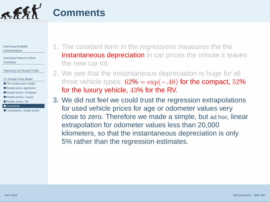
3. We did not feel we could trust the regression extrapolationsfor used vehicle prices for age or odometer values veryclose to zero. Therefore we made a simple, but ad hoc, linearextrapolation for odometer values less than 20,000kilometers, so that the instantaneous depreciation is only5% rather than the regression estimates.
4. However predictions of the optimal replacement policy arenot sensitive to our assumptions about the precise shape ofthe depreciation curve for cars with odometer values of lessthan 20,000 kilometers.

Improving Disability
Determinations
Improving Return to Work
Incentives
Improving Car Rental Profits
3.2 Resale Price Model
● The resale price model
● Resale price regression
● Resale prices: Compact
● Resale prices: Luxury
● Resale prices: RV
● Comments
● Conclusions: resale prices
John Rust Bad Decisions - slide #83
Conclusions: resale prices
1. Conclusion 1: beyond age and odometer value (andimplicitly the car’s characteristics, as represented by itsmake and model), there are few other significantexplanatory variables for the resale value of a car.
2. Our regressions can explain only between 40 to 50% of thevariation in the resale values of the cars the company sells:there is a lot of “residual variance” that leads one car to sellfor much more than another car that from our standpoint is“observationally equivalent” to it.
3. Conclusion 2: the rapid initial depreciation implies thatvehicle replacement is a significant investment that can beamortized by keeping the vehicle sufficiently long beforenext replacement.


Improving Disability
Determinations
Improving Return to Work
Incentives
Improving Car Rental Profits
3.3 Vehicle Usage Model
● Vehicle Usage Model
● Lifetime Usage Identities
● Estimating the Usage Model
John Rust Bad Decisions - slide #85
Vehicle Usage Model
1. As noted above, the firm frequently does not accuratelyrecord in/out odometer values for rental spells.
2. To circumvent this problem we make a functional formassumption. Let F (o′|o, d, r) denote the conditionaldistribution of odometer value of a car returning from arental contract of type r that lasted d days when the outodometer value was o.
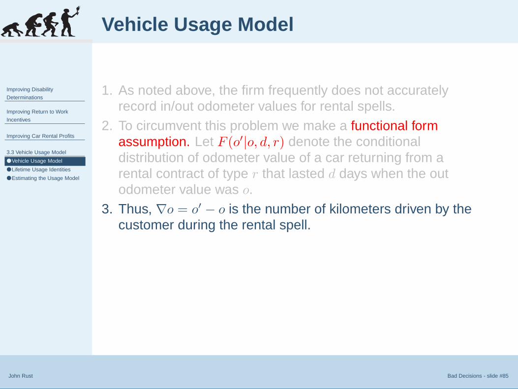
3. Thus, ∇o = o′ − o is the number of kilometers driven by thecustomer during the rental spell.
4. We assume that the number of kilometers travelled eachday by a rental customer are IID draws from an exponentialdistribution with parameter λr.
5. Conditional on spell length d, it follows that F (o′|d, r) is agamma distribution, since a sum of IID exponential randomvariables has a gamma distribution.
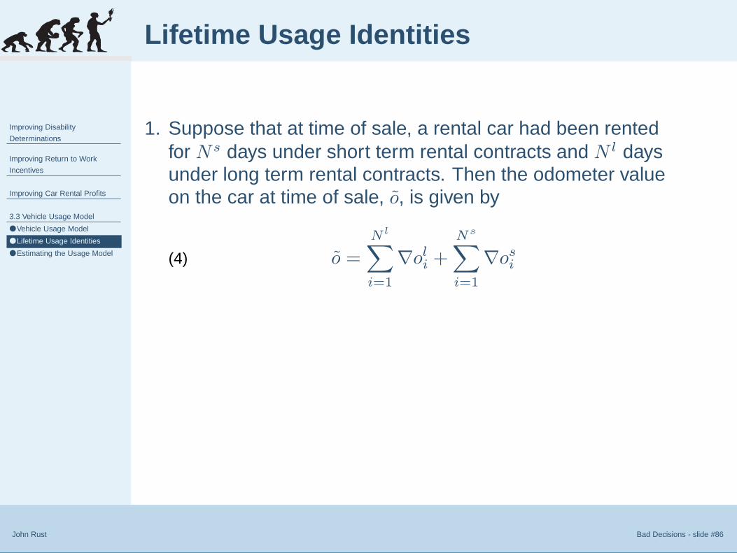
Improving Disability
Determinations
Improving Return to Work
Incentives
Improving Car Rental Profits
3.3 Vehicle Usage Model
● Vehicle Usage Model
● Lifetime Usage Identities
● Estimating the Usage Model
John Rust Bad Decisions - slide #86
Lifetime Usage Identities
1. Suppose that at time of sale, a rental car had been rentedfor Ns days under short term rental contracts and N l daysunder long term rental contracts. Then the odometer valueon the car at time of sale, o, is given by
o =N l∑i=1
∇oli +
Ns∑i=1
∇osi(4)
2. Thus, we have
E{o|N l, Ns} = λ1Nl + λ2N
s.(5)
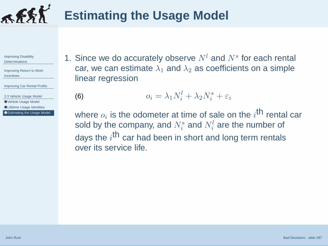
Improving Disability
Determinations
Improving Return to Work
Incentives
Improving Car Rental Profits
3.3 Vehicle Usage Model
● Vehicle Usage Model
● Lifetime Usage Identities
● Estimating the Usage Model
John Rust Bad Decisions - slide #87
Estimating the Usage Model
1. Since we do accurately observe N l and Ns for each rentalcar, we can estimate λ1 and λ2 as coefficients on a simplelinear regression
oi = λ1Nli + λ2N
si + εi(6)
where oi is the odometer at time of sale on the ith rental carsold by the company, and Ns
i and N li are the number of
days the ith car had been in short and long term rentalsover its service life.
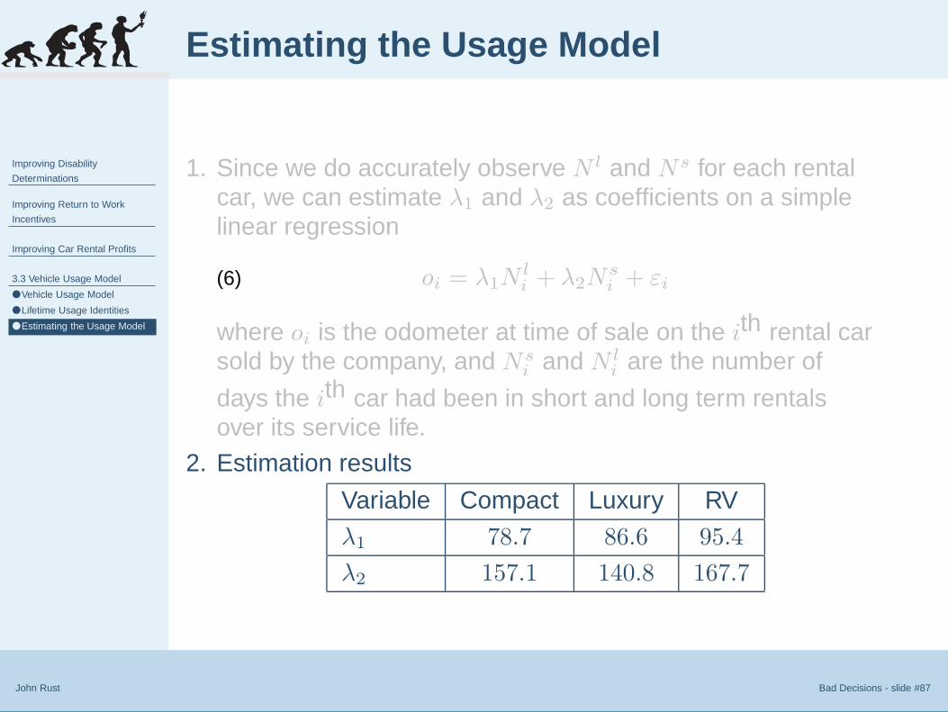
2. Estimation results
Variable Compact Luxury RV
λ1 78.7 86.6 95.4
λ2 157.1 140.8 167.7


Improving Disability
Determinations
Improving Return to Work
Incentives
Improving Car Rental Profits
3.4 The Replacement Model
● The Replacement Decision
● Logit Estimation Results
● Replacement Conclusions
● Odometer at Sale: Compact
● Age at Sale: Compact
● Odometer at Sale: Luxury
● Age at Sale: Luxury
● Odometer at Sale: RV
● Age at Sale: RV
John Rust Bad Decisions - slide #89
The Replacement Decision
1. Let st denote a binary variable for the selling decision withst = 1 if the company sells the car and st = 0 if the companykeeps the car.
2. We estimated the company’s decision to sell the car using abinary logit model
Pr {st = 1|xt} =exp{xtθ}
1 + exp{xtθ}.(7)
3. Among the variables in the vector xt are the vehicle’s ageand predicted odometer value (based on the regressionestimate ot using the observed values of N l
t and Nst from
the rental contract data, as discussed above), duration inthe lot, average daily maintenance costs, and utilization rate.
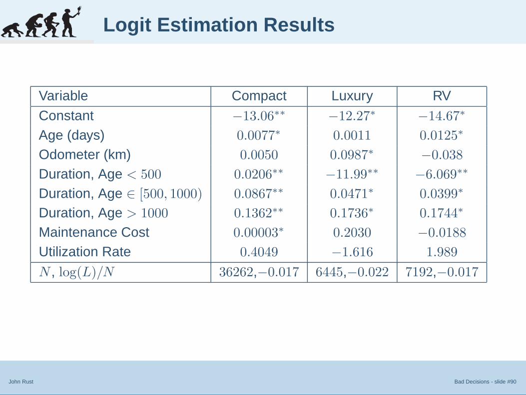
John Rust Bad Decisions - slide #90
Logit Estimation Results
Variable Compact Luxury RV
Constant −13.06∗∗ −12.27∗ −14.67∗
Age (days) 0.0077∗ 0.0011 0.0125∗
Odometer (km) 0.0050 0.0987∗ −0.038
Duration, Age < 500 0.0206∗∗ −11.99∗∗ −6.069∗∗
Duration, Age ∈ [500, 1000) 0.0867∗∗ 0.0471∗ 0.0399∗
Duration, Age > 1000 0.1362∗∗ 0.1736∗ 0.1744∗
Maintenance Cost 0.00003∗ 0.2030 −0.0188
Utilization Rate 0.4049 −1.616 1.989
N , log(L)/N 36262,−0.017 6445,−0.022 7192,−0.017

Improving Disability
Determinations
Improving Return to Work
Incentives
Improving Car Rental Profits
3.4 The Replacement Model
● The Replacement Decision
● Logit Estimation Results
● Replacement Conclusions
● Odometer at Sale: Compact
● Age at Sale: Compact
● Odometer at Sale: Luxury
● Age at Sale: Luxury
● Odometer at Sale: RV
● Age at Sale: RV
John Rust Bad Decisions - slide #91
Replacement Conclusions
1. Due to the collinearity between age and odometer value, itis difficult to identify the separate effects of age versusodometer value on the firm’s decision to sell a vehicle.
2. Model fits about as well if age is excluded from the logit.
3. Besides age and odometer, the only variable whosecoefficient estimates are statistically significant and hassigns that are (generally) consistent with our a prioriexpectations is duration.
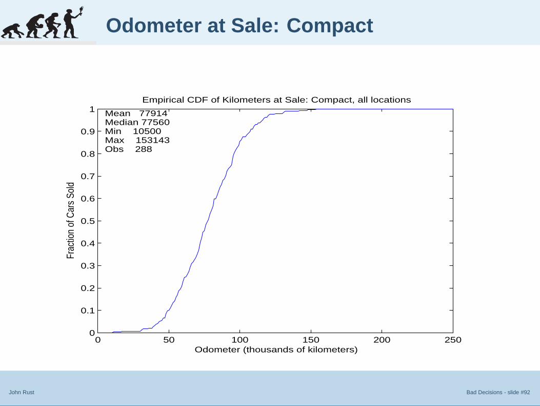
John Rust Bad Decisions - slide #92
Odometer at Sale: Compact
0 50 100 150 200 2500
0.1
0.2
0.3
0.4
0.5
0.6
0.7
0.8
0.9
1
Odometer (thousands of kilometers)
Frac
tion
of C
ars
Sold
Empirical CDF of Kilometers at Sale: Compact, all locations
Mean 77914Median 77560Min 10500Max 153143Obs 288

John Rust Bad Decisions - slide #93
Age at Sale: Compact
0 1 2 3 4 5 60
0.1
0.2
0.3
0.4
0.5
0.6
0.7
0.8
0.9
1
Age of Car (years)
Frac
tion
of C
ars
Sold
Empirical CDF of Age at Sale: Compact, all locations
Mean 2.81Median 2.84Min 1.53Max 4.03Obs 288

John Rust Bad Decisions - slide #94
Odometer at Sale: Luxury
0 50 100 150 200 2500
0.1
0.2
0.3
0.4
0.5
0.6
0.7
0.8
0.9
1
Odometer (thousands of kilometers)
Frac
tion
of C
ars
Sold
Empirical CDF of Kilometers at Sale: Luxury 2, all locations
Mean 74684Median 71300Min 35000Max 187800Obs 91
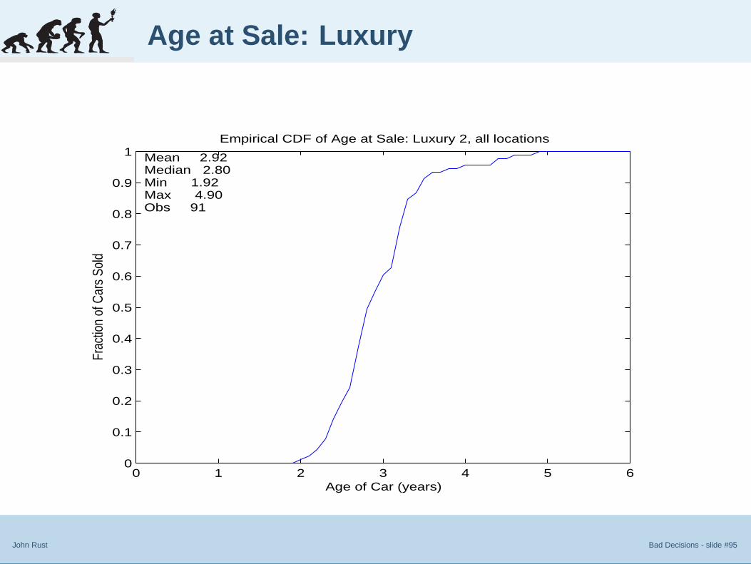
John Rust Bad Decisions - slide #95
Age at Sale: Luxury
0 1 2 3 4 5 60
0.1
0.2
0.3
0.4
0.5
0.6
0.7
0.8
0.9
1
Age of Car (years)
Frac
tion
of C
ars
Sold
Empirical CDF of Age at Sale: Luxury 2, all locations
Mean 2.92Median 2.80Min 1.92Max 4.90Obs 91

John Rust Bad Decisions - slide #96
Odometer at Sale: RV
0 50 100 150 200 2500
0.1
0.2
0.3
0.4
0.5
0.6
0.7
0.8
0.9
1
Odometer (thousands of kilometers)
Frac
tion
of C
ars
Sold
Empirical CDF of Kilometers at Sale: RV, all locations
Mean 88829Median 91200Min 38000Max 163860Obs 41
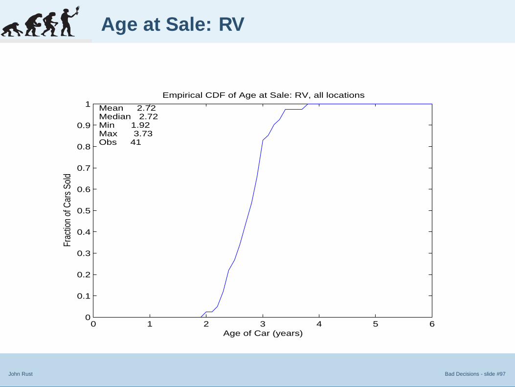
John Rust Bad Decisions - slide #97
Age at Sale: RV
0 1 2 3 4 5 60
0.1
0.2
0.3
0.4
0.5
0.6
0.7
0.8
0.9
1
Age of Car (years)
Frac
tion
of C
ars
Sold
Empirical CDF of Age at Sale: RV, all locations
Mean 2.72Median 2.72Min 1.92Max 3.73Obs 41


Improving Disability
Determinations
Improving Return to Work
Incentives
Improving Car Rental Profits
3.5 The Duration Model
● Estimated Spell Durations
● Rental Durations: Compact
● Lot Spell Durations
● Lot Durations: Compact
John Rust Bad Decisions - slide #99
Estimated Spell Durations
1. The remaining objects to be estimated to implement oureconometric model are the spell durations and the statetransition probabilities.
2. Let let h(d, r) denote the hazard rate for the rental state r.
3. The duration distribtion f(d|r) implied by the hazard functionh(d, r) is
f(d|r) =
{f(1|r) = h(0, r)
f(d|r) =∏d−2
j=0 [1 − h(j, r)]h(d − 1, r) d ≥ 2
(8)
4. Since we have sufficiently many observations of rentalspells, we were able to estimate the hazard functions forthese spells non-parametrically.

John Rust Bad Decisions - slide #100
Rental Durations: Compact
0 5 10 15 20 25 30 350
0.1
0.2
0.3
0.4
0.5
0.6
0.7
Duration of rental spell (days)
Cond
itiona
l pro
babi
lity o
f lea
ving
spel
l
Distribution of rental spells, Compact, all locations
Long term rentalShort term rental

Improving Disability
Determinations
Improving Return to Work
Incentives
Improving Car Rental Profits
3.5 The Duration Model
● Estimated Spell Durations
● Rental Durations: Compact
● Lot Spell Durations
● Lot Durations: Compact
John Rust Bad Decisions - slide #101
Lot Spell Durations
1. We have far fewer observations on lot spell durations,especially for type 3 lot spells due to the high probability ofroll overs in longer term contracts.
2. With fewer observations, our nonparametrically estimatedhazard functions are quite jagged.
3. Also, unlike rental contracts, there is no a priori upper boundon the duration of a lot spell.
4. As a result we needed some method of extrapolation topredict durations given that we have only a small number ofcases with extremely long lot durations.
5. We assume that the hazard function is constant after d = 31days, which implies that the upper tail for the distribution oflot spells is geometric.
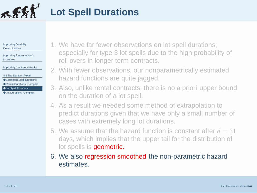
6. We also regression smoothed the non-parametric hazardestimates.

John Rust Bad Decisions - slide #102
Lot Durations: Compact
0 5 10 15 20 25 30 350
0.05
0.1
0.15
0.2
0.25
0.3
0.35
0.4
Duration of lot spells (days)
Cond
itiona
l pro
babi
lity o
f lea
ving
spel
l
Lot Spell Hazard Functions for Compact, all locations
Smoothed hazard: previous long term rentalNonparametric hazard: previous long term rentalSmoothed hazard: previous short term rentalNonparametric hazard: previous short term rental


Improving Disability
Determinations
Improving Return to Work
Incentives
Improving Car Rental Profits
3.6 Transition Models
● Transition Probabilities
● Functional Forms
● Trinomial Logit Estimates
● Lot Spell Transitions
● Binomial Logit Estimates
● Conclusions
John Rust Bad Decisions - slide #104
Transition Probabilities
1. When a spell in a given rental state ends, there is atransition to a new rental state.
2. Let π(r′|r, d, o) denote probability the new rental state for acar will be r′ given that the current rental state is r, theodometer value is o, and the duration in state r is d.
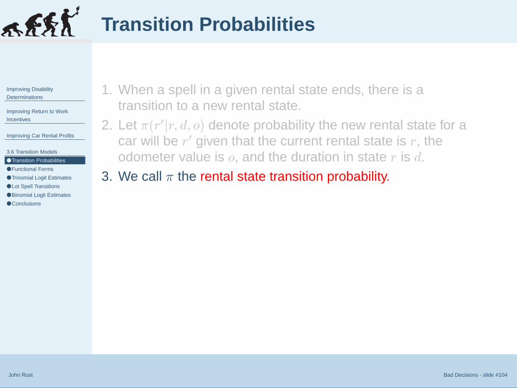
3. We call π the rental state transition probability.
4. We rule out “self transitions” to lot spells, i.e. π(r|r, d, o) = 0for r > 2.
5. However for rental spells, there is a conceptual distinctionbetween a rental spell that terminates with an immediatetransition to a new rental spell versus the case where anexisting rental contract continues for one more day.
6. The former case can be viewed as an immediate “roll over”of one rental contract to another one.

Improving Disability
Determinations
Improving Return to Work
Incentives
Improving Car Rental Profits
3.6 Transition Models
● Transition Probabilities
● Functional Forms
● Trinomial Logit Estimates
● Lot Spell Transitions
● Binomial Logit Estimates
● Conclusions
John Rust Bad Decisions - slide #105
Functional Forms
1. Since there are three possible destination states fortransitions out of rental spells (i.e. long term contract, shortterm contract, or lot spell), we used a trinomial logit model toestimate these probabilities.
π(r′|r, d, o) =exp{v(r, d, o)θr′}∑
ρ∈{1,2,l(r)} exp{v(r, d, o)θρ},(9)
2. v(r, d, o) is a vector-valued function of the variables (r, d, o)and θρ is an alternative-specific vector of parameters, forρ = {1, 2, l(r)} (where l(r) denotes a lot spell, either of type3 if r = 1 or type 4 if r = 2) with the same dimension as v.
3. As is well known, it is not possible to identify all three of theθρ vectors. Therefore we make an identifying normalizationthat θ1 = 0, i.e. we normalized the parameters for transitionto long term contract to zero.
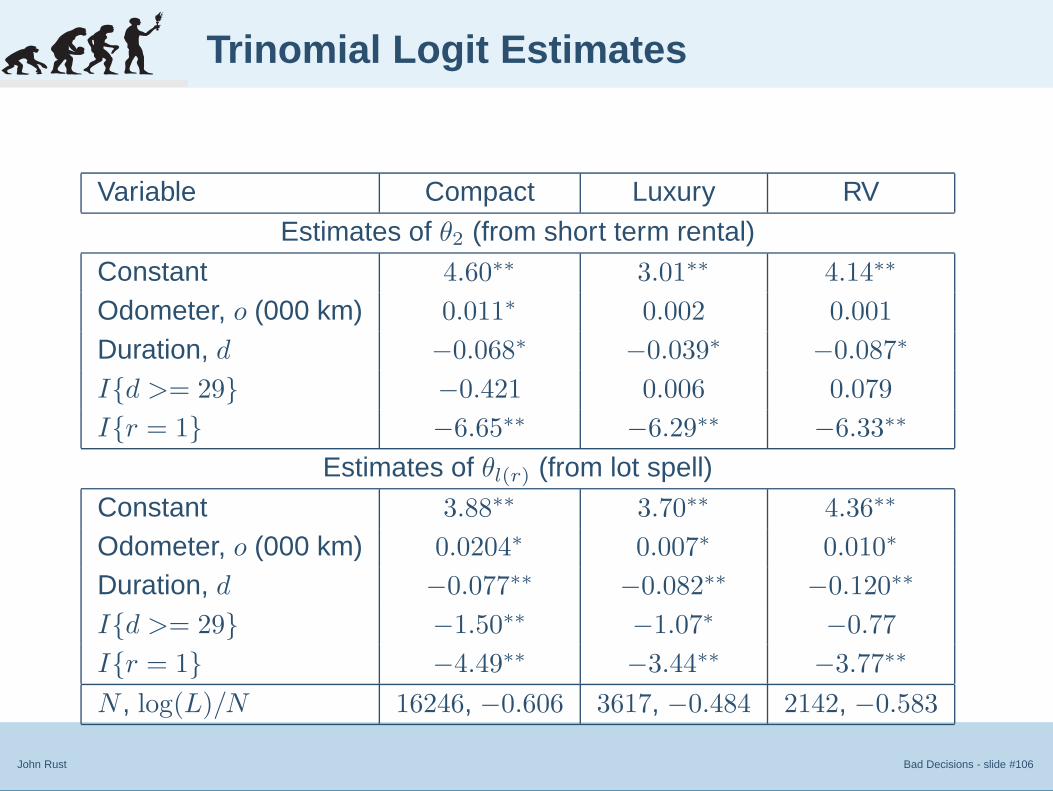
John Rust Bad Decisions - slide #106
Trinomial Logit Estimates
Variable Compact Luxury RV
Estimates of θ2 (from short term rental)
Constant 4.60∗∗ 3.01∗∗ 4.14∗∗
Odometer, o (000 km) 0.011∗ 0.002 0.001
Duration, d −0.068∗ −0.039∗ −0.087∗
I{d >= 29} −0.421 0.006 0.079
I{r = 1} −6.65∗∗ −6.29∗∗ −6.33∗∗
Estimates of θl(r) (from lot spell)
Constant 3.88∗∗ 3.70∗∗ 4.36∗∗
Odometer, o (000 km) 0.0204∗ 0.007∗ 0.010∗
Duration, d −0.077∗∗ −0.082∗∗ −0.120∗∗
I{d >= 29} −1.50∗∗ −1.07∗ −0.77
I{r = 1} −4.49∗∗ −3.44∗∗ −3.77∗∗
N , log(L)/N 16246, −0.606 3617, −0.484 2142, −0.583

Improving Disability
Determinations
Improving Return to Work
Incentives
Improving Car Rental Profits
3.6 Transition Models
● Transition Probabilities
● Functional Forms
● Trinomial Logit Estimates
● Lot Spell Transitions
● Binomial Logit Estimates
● Conclusions
John Rust Bad Decisions - slide #107
Lot Spell Transitions
1. For transitions out of lot spells, since we have ruled out thepossibility of “self-transitions” there are only two possibledestinations: long term rental spells and short term rentalspells.
2. We use a binomial logit model to estimate these probabilities
π(r′ = 1|r, d, o) =exp{v(o, d)θr}
1 + exp{v(o, d)θr}, r ∈ {3, 4}(10)
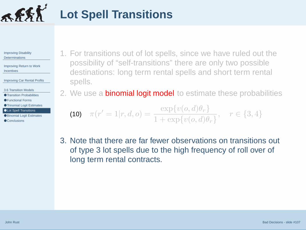
3. Note that there are far fewer observations on transitions outof type 3 lot spells due to the high frequency of roll over oflong term rental contracts.
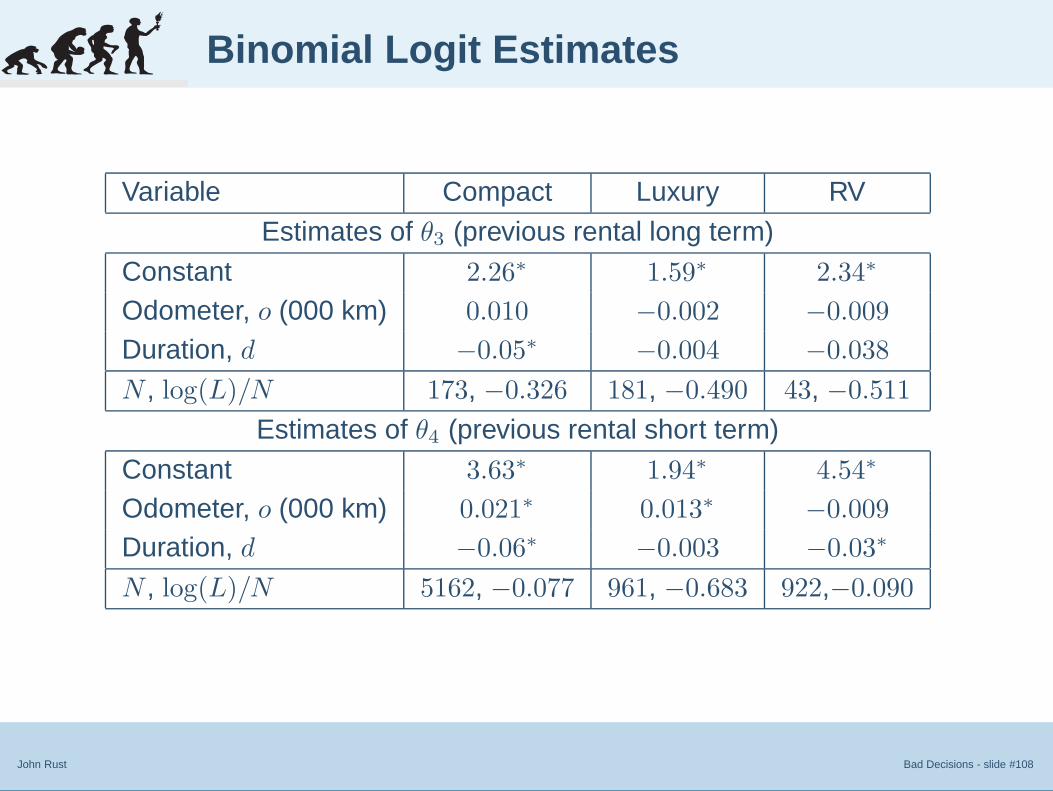
John Rust Bad Decisions - slide #108
Binomial Logit Estimates
Variable Compact Luxury RV
Estimates of θ3 (previous rental long term)
Constant 2.26∗ 1.59∗ 2.34∗
Odometer, o (000 km) 0.010 −0.002 −0.009
Duration, d −0.05∗ −0.004 −0.038
N , log(L)/N 173, −0.326 181, −0.490 43, −0.511
Estimates of θ4 (previous rental short term)
Constant 3.63∗ 1.94∗ 4.54∗
Odometer, o (000 km) 0.021∗ 0.013∗ −0.009
Duration, d −0.06∗ −0.003 −0.03∗
N , log(L)/N 5162, −0.077 961, −0.683 922,−0.090

Improving Disability
Determinations
Improving Return to Work
Incentives
Improving Car Rental Profits
3.6 Transition Models
● Transition Probabilities
● Functional Forms
● Trinomial Logit Estimates
● Lot Spell Transitions
● Binomial Logit Estimates
● Conclusions
John Rust Bad Decisions - slide #109
Conclusions
■ There are two key points to take away from the transitionprobability estimates
1. for all car types, there is a very high probability that carswill be initially rented in long term contracts,
2. the results provide clear evidence of “contract ageeffects”.
■ That is, as the odometer value increases (i.e. the age of thecar increases) the probability of transitions into long termrental contracts decreases and the probability of transitionsinto short term rental contracts increases.
■ However we find no other aging effects in spell durations or inmaintenance costs.


John Rust Bad Decisions - slide #111
Transition from Long Term
0 50 100 1500
0.1
0.2
0.3
0.4
0.5
0.6
0.7
0.8
0.9
1Estimated Transition Probabilities from Long Term Rental Spell
Odometer, (thousands of kilometers)
Prob
abilit
y of
New
Spe
ll
Long Term Rental SpellShort Term Rental SpellLot Spell

John Rust Bad Decisions - slide #112
Transition from Short Term
0 50 100 1500
0.1
0.2
0.3
0.4
0.5
0.6
0.7
0.8
0.9Estimated Transition Probabilities from Short Term Rental Spell
Odometer, (thousands of kilometers)
Prob
abilit
y of
New
Spe
ll
Long Term Rental SpellShort Term Rental SpellLot Spell

John Rust Bad Decisions - slide #113
Transition from Lot Type 3
0 50 100 1500
0.05
0.1
0.15
0.2
0.25
0.3
0.35Estimated Transition Probabilities from Lot Spell, Type 3
Odometer, (thousands of kilometers)
Prob
abilit
y of
Ent
erin
g Lo
ng T
erm
Ren
tal S
pell
d=1d=10d=30

John Rust Bad Decisions - slide #114
Transition from Lot Type 4
0 50 100 1500
0.02
0.04
0.06
0.08
0.1
0.12
0.14
0.16Estimated Transition Probabilities from Lot Spell, Type 4
Odometer, (thousands of kilometers)
Prob
abilit
y of
Ent
erin
g Lo
ng T
erm
Ren
tal S
pell
d=1d=10d=30


John Rust Bad Decisions - slide #116
No Aging in Maintenance
0 20 40 60 80 100 120−0.5
0
0.5
1
1.5
2
Predicted Odometer (thousands of kilometers)
Dai
ly M
aint
enan
ce C
ost
Scatterplot of Daily Maintenance Costs for Compact, all locations
Mean 0.06Std dev 0.54Observations 13079
0 200 400 600 800 1000 1200−0.5
0
0.5
1
1.5
2
Vehicle Age (days)D
aily
Mai
nten
ance
Cos
t
Scatterplot of Daily Maintenance Costs for Compact, all locations
Mean 0.06Std dev 0.54Observations 13079

John Rust Bad Decisions - slide #117
No Aging in Rental Durations
0 20 40 60 80 100 1200
5
10
15
20
25
30
35
40
Predicted Odometer (thousands of kilometers)
Dur
atio
n of
Ren
tal S
pell
(Day
s)
Scatterplot of Short Term Rental Durations for Compact, all locations
Mean 2.5Std dev 5.1Observations 10390
0 20 40 60 80 100 1200
5
10
15
20
25
30
35
40
Predicted Odometer (thousands of kilometers)D
urat
ion
of R
enta
l Spe
ll (D
ays)
Scatterplot of Long Term Rental Durations for Compact, all locations
Mean 28.8Std dev 5.4Observations 2689

John Rust Bad Decisions - slide #118
No Aging in Lot Durations
0 20 40 60 80 100 1200
5
10
15
20
25
30
35
40
45
50
Predicted Odometer (thousands of kilometers)
Dur
atio
n of
Lot
Spe
ll (d
ays)
Durations of Lot Spells for Compact, all locations, Previous Rental Spell was Long Term
Mean duration 9.3Mean odometer 43.0Observations 174
0 20 40 60 80 100 1200
10
20
30
40
50
60
70
80
90
Predicted Odometer (thousands of kilometers)D
urat
ion
of L
ot S
pell
(day
s)
Durations of Lot Spells for Compact, all locations, Previous Rental Spell was Short Term
Mean duration 3.3Mean odometer 41.6Observations 5165


John Rust Bad Decisions - slide #120
Simulated Histories
100 200 300 400 500 600 700 800 900 1000 11000
1
2Compact, all locations realization 43 (service life: 1171 days, IRR=69.4)
Day in Life of Car
Rent
al St
ate
100 200 300 400 500 600 700 800 9000
1
2Luxury 2, all locations realization 87 (service life: 979 days, IRR=50.1)
Day in Life of Car
Rent
al St
ate
100 200 300 400 500 600 7000
1
2RV, all locations realiation 88 (service life: 705 days, IRR=44.6)
Day in Life of Car
Rent
al St
ate


John Rust Bad Decisions - slide #122
Odometer at Replacement
40 60 80 100 120 140 160 1800
0.002
0.004
0.006
0.008
0.01
0.012
0.014
0.016
0.018
0.02
Kilometers at Sale (in thousands) Luxury 2, all locations
Dens
ity
Distribution of Kilometers at Sale (in thousands) Luxury 2, all locations
Actual
Mean 74.7
Median 71.3
Minimum 35.0
Maximum 187.8
Std dev 24.8
N 91
Simulated
Mean 71.1
Median 69.4
Minimum 31.5
Maximum 139.4
Std dev 20.8
N 100
ActualSimulated

John Rust Bad Decisions - slide #123
Age at Replacement
1 1.5 2 2.5 3 3.5 4 4.5 50
0.1
0.2
0.3
0.4
0.5
0.6
0.7
0.8
0.9
1
Age at Sale (Years) Luxury 2, all locations
Dens
ity
Distribution of Age at Sale (Years) Luxury 2, all locations
Actual
Mean 2.7
Median 2.6
Minimum 1.9
Maximum 4.0
Std dev 0.4
N 40
Simulated
Mean 2.6
Median 2.5
Minimum 0.8
Maximum 5.1
Std dev 0.8
N 100
ActualSimulated


John Rust Bad Decisions - slide #125
Number of Long Term Rentals
5 10 15 20 25 30 35 40 450
0.005
0.01
0.015
0.02
0.025
0.03
0.035
0.04
0.045
0.05
Number of Long Term Rentals Luxury 2, all locations
Dens
ity
Distribution of Number of Long Term Rentals Luxury 2, all locations
Actual
Mean 24.7
Median 24.0
Minimum 6.0
Maximum 48.0
Std dev 9.3
N 40
Simulated
Mean 22.8
Median 23.0
Minimum 2.0
Maximum 39.0
Std dev 7.0
N 100
ActualSimulated
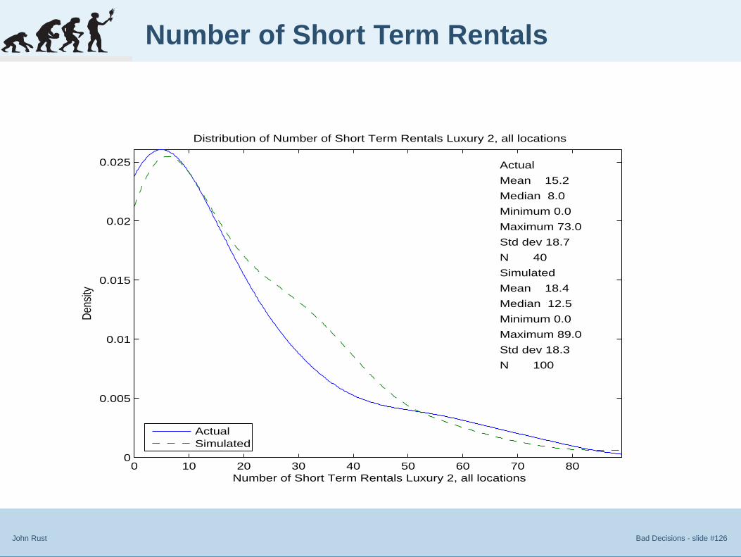
John Rust Bad Decisions - slide #126
Number of Short Term Rentals
0 10 20 30 40 50 60 70 800
0.005
0.01
0.015
0.02
0.025
Number of Short Term Rentals Luxury 2, all locations
Dens
ity
Distribution of Number of Short Term Rentals Luxury 2, all locations
Actual
Mean 15.2
Median 8.0
Minimum 0.0
Maximum 73.0
Std dev 18.7
N 40
Simulated
Mean 18.4
Median 12.5
Minimum 0.0
Maximum 89.0
Std dev 18.3
N 100
ActualSimulated

John Rust Bad Decisions - slide #127
Number of Lot Spells
10 20 30 40 50 600
0.005
0.01
0.015
0.02
0.025
0.03
0.035
Number of Lot Spells Luxury 2, all locations
Dens
ity
Distribution of Number of Lot Spells Luxury 2, all locations
Actual
Mean 13.9
Median 9.0
Minimum 2.0
Maximum 59.0
Std dev 14.2
N 40
Simulated
Mean 14.2
Median 11.0
Minimum 1.0
Maximum 69.0
Std dev 12.8
N 100
ActualSimulated


John Rust Bad Decisions - slide #129
Days in Long Term Rentals
200 400 600 800 1000 1200 14000
0.2
0.4
0.6
0.8
1
1.2
1.4
1.6
x 10−3
Days in Long Term Rentals Luxury 2, all locations
Dens
ity
Distribution of Days in Long Term Rentals Luxury 2, all locations
Actual
Mean 696.8
Median 715.0
Minimum 146.0
Maximum 1252.0
Std dev 270.7
N 40
Simulated
Mean 642.6
Median 628.5
Minimum 174.0
Maximum 1454.0
Std dev 215.2
N 100
ActualSimulated
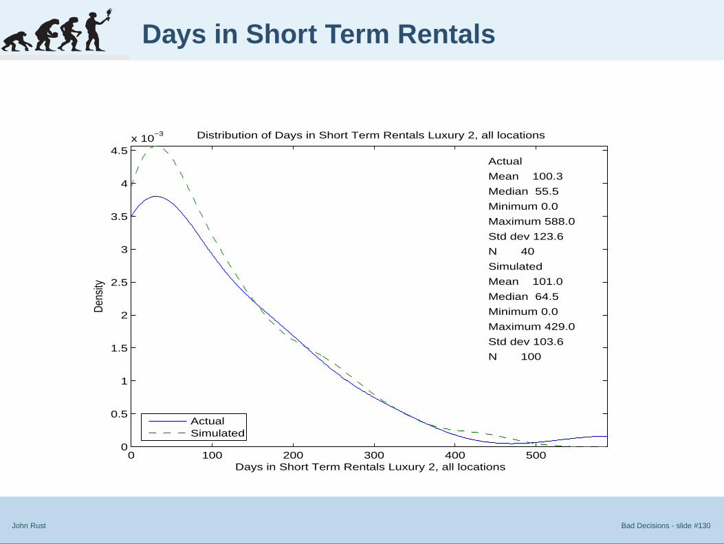
John Rust Bad Decisions - slide #130
Days in Short Term Rentals
0 100 200 300 400 5000
0.5
1
1.5
2
2.5
3
3.5
4
4.5x 10
−3
Days in Short Term Rentals Luxury 2, all locations
Dens
ity
Distribution of Days in Short Term Rentals Luxury 2, all locations
Actual
Mean 100.3
Median 55.5
Minimum 0.0
Maximum 588.0
Std dev 123.6
N 40
Simulated
Mean 101.0
Median 64.5
Minimum 0.0
Maximum 429.0
Std dev 103.6
N 100
ActualSimulated

John Rust Bad Decisions - slide #131
Days in Lot Spells
100 200 300 400 500 6000
0.5
1
1.5
2
2.5
3
3.5
x 10−3
Days on the Lot Luxury 2, all locations
Dens
ity
Distribution of Days on the Lot Luxury 2, all locations
Actual
Mean 192.6
Median 144.0
Minimum 8.0
Maximum 544.0
Std dev 141.2
N 40
Simulated
Mean 129.2
Median 103.0
Minimum 3.0
Maximum 615.0
Std dev 109.8
N 100
ActualSimulated


John Rust Bad Decisions - slide #133
Vehicle Sales Proceeds
0.8 0.9 1 1.1 1.2 1.3 1.4 1.5 1.6
x 104
0
0.5
1
1.5
2
2.5
x 10−4
Revenue from Sale of Car Luxury 2, all locations
Dens
ity
Distribution of Revenue from Sale of Car Luxury 2, all locations
Actual
Mean 12283.2
Median 12180.0
Minimum 7500.0
Maximum 16550.0
Std dev 1666.6
N 40
Simulated
Mean 12109.4
Median 12197.7
Minimum 7954.2
Maximum 16881.9
Std dev 1709.8
N 100
ActualSimulated

John Rust Bad Decisions - slide #134
Maintenance Costs
500 1000 1500 2000 2500 3000 3500 4000 4500 5000 55000
0.2
0.4
0.6
0.8
1
1.2
x 10−3
Total Maintenance Costs Luxury 2, all locations
Dens
ity
Distribution of Total Maintenance Costs Luxury 2, all locations
Actual
Mean 956.4
Median 748.9
Minimum 135.0
Maximum 5866.7
Std dev 932.1
N 40
Simulated
Mean 1085.7
Median 1068.8
Minimum 471.9
Maximum 2348.8
Std dev 359.6
N 100
ActualSimulated

John Rust Bad Decisions - slide #135
Long Term Rental Revenues
1 2 3 4 5 6
x 104
0
0.5
1
1.5
2
2.5
3
3.5
x 10−5
Revenue from Long Term Rentals Luxury 2, all locations
Dens
ity
Distribution of Revenue from Long Term Rentals Luxury 2, all locations
Actual
Mean 28206.9
Median 28154.2
Minimum 6320.9
Maximum 50427.3
Std dev 10631.9
N 40
Simulated
Mean 28621.0
Median 28126.8
Minimum 7880.7
Maximum 65005.2
Std dev 9605.9
N 100
ActualSimulated
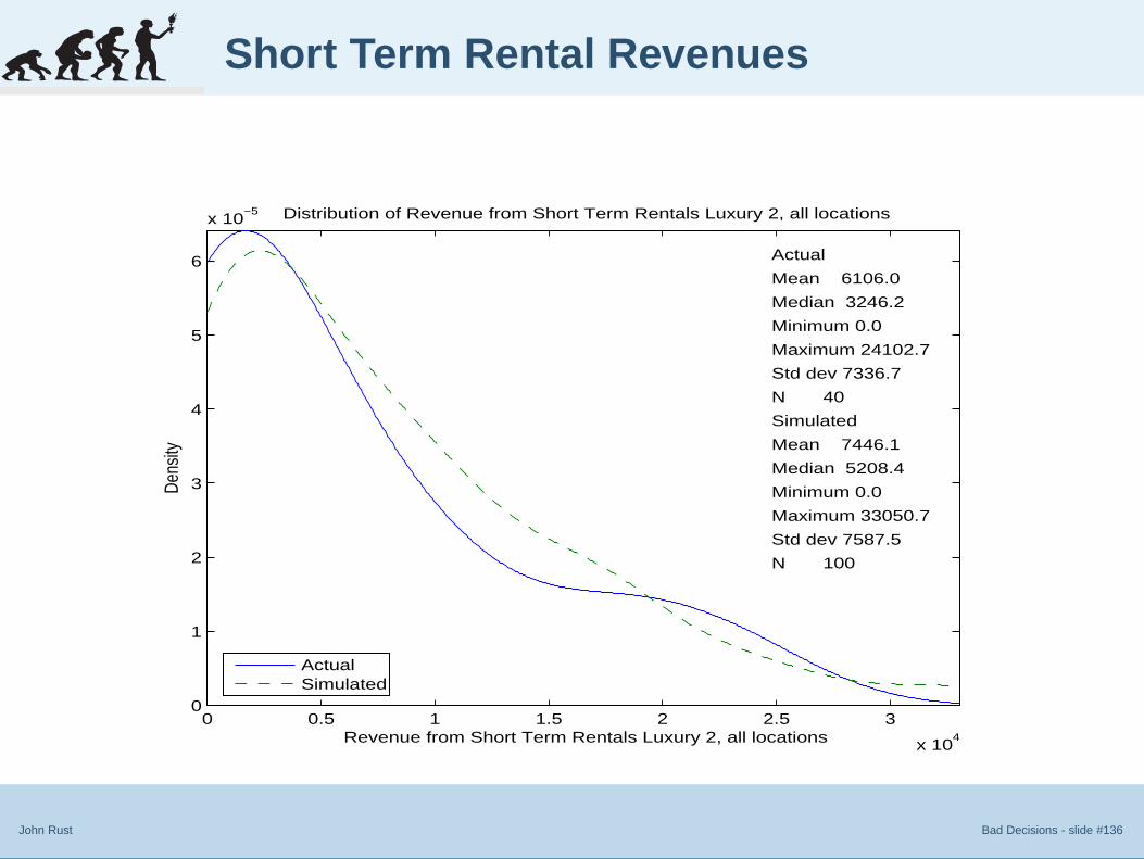
John Rust Bad Decisions - slide #136
Short Term Rental Revenues
0 0.5 1 1.5 2 2.5 3
x 104
0
1
2
3
4
5
6
x 10−5
Revenue from Short Term Rentals Luxury 2, all locations
Dens
ity
Distribution of Revenue from Short Term Rentals Luxury 2, all locations
Actual
Mean 6106.0
Median 3246.2
Minimum 0.0
Maximum 24102.7
Std dev 7336.7
N 40
Simulated
Mean 7446.1
Median 5208.4
Minimum 0.0
Maximum 33050.7
Std dev 7587.5
N 100
ActualSimulated

John Rust Bad Decisions - slide #137
Total Profits
0.5 1 1.5 2 2.5 3 3.5 4 4.5 5
x 104
0
1
2
3
4
5
6
x 10−5
Total Profits Luxury 2, all locations
Dens
ity
Distribution of Total Profits Luxury 2, all locations
Actual
Mean 22244.3
Median 21868.1
Minimum 10942.0
Maximum 37184.1
Std dev 6223.7
N 40
Simulated
Mean 22212.7
Median 22403.1
Minimum 3979.2
Maximum 51391.9
Std dev 9608.2
N 100
ActualSimulated

John Rust Bad Decisions - slide #138
Internal Rates of Return
20 30 40 50 60 700
0.01
0.02
0.03
0.04
0.05
Internal Rate of Return (%) Luxury 2, all locations
Dens
ity
Distribution of Internal Rate of Return (%) Luxury 2, all locations
Actual
Mean 49.2
Median 48.7
Minimum 28.6
Maximum 79.5
Std dev 10.4
N 40
Simulated
Mean 47.1
Median 48.4
Minimum 18.4
Maximum 60.5
Std dev 6.9
N 100
ActualSimulated


Improving Disability
Determinations
Improving Return to Work
Incentives
Improving Car Rental Profits
5 Optimal Replacement Theory
● Optimal Stopping Theory
● Dynamic Programming
● Valuing Alternative Policies
John Rust Bad Decisions - slide #140
Optimal Stopping Theory
1. While it is possible to evaluate specific hypotheticalalternatives to the company’s status quo operating policyusing simulation methods similar to the previous section,there are more efficient methods available for searching overall possible policies to find the optimal replacement policy.
2. Mathematically, the optimal replacement problem isequivalent to a specific type of optimal stopping problemknown as a regenerative optimal stopping problem (seeRust, 1987).
3. The term “regenerative” is used, since the decision toreplace a vehicle does not stop or end the decision process,but rather results in a “regeneration” or “rebirth”, i.e. areplacement of an old vehicle by a brand new one.

Improving Disability
Determinations
Improving Return to Work
Incentives
Improving Car Rental Profits
5 Optimal Replacement Theory
● Optimal Stopping Theory
● Dynamic Programming
● Valuing Alternative Policies
John Rust Bad Decisions - slide #141
Dynamic Programming
1. We use the method of dynamic programming to formulateand solve the optimal stopping problem.
2. We show that the optimal strategy takes the form of athreshold rule, i.e. the optimal time to replace a car occurswhen its odometer value o exceeds a threshold valueo(d, r, τ) that depends on the current rental state r, theduration in that state d, and the car type τ .
3. Using numerical methods, we solve the dynamicprogramming problem and calculate the optimal stoppingthresholds o(d, r, τ).
4. We also compute the optimal value functions V (r, d, o, τ).This function provides the expected discounted profits (overan infinite horizon) under the optimal replacement policy fora vehicle that is in state (r, d, o).

Improving Disability
Determinations
Improving Return to Work
Incentives
Improving Car Rental Profits
5 Optimal Replacement Theory
● Optimal Stopping Theory
● Dynamic Programming
● Valuing Alternative Policies
John Rust Bad Decisions - slide #142
Valuing Alternative Policies
1. It is also possible to compute the value of any alternativeoperating strategy µ, which can include mixed orprobabilistic operating strategies where the decision toreplace a car is given by a conditional probability distributionµ(r, d, o, τ).
2. Let Vµ(r, d, o, τ) denote the expected discounted profits(again over an infinite horizon) under the alternativereplacment policy µ.
3. We will calculate both V and Vµ where µ is anapproximation to the company’s status quo operating policy.
4. The difference V (r, d, o, τ) − Vµ(r, d, o, τ) will represent ourestimate of the gain in profits from adopting an optimalreplacement policy.
5. We will show that the optimal policy entails keeping carssignificantly longer than the company currently keeps them.

Improving Disability
Determinations
Improving Return to Work
Incentives
Improving Car Rental Profits
6 Numerical Results
● No Extrapolation Case
● The Pessimistic Case
● Multiplication Factors
John Rust Bad Decisions - slide #144
No Extrapolation Case
1. As we noted above, if we solve the regenerative optimalstopping problem under the assumption that the only agingeffects are 1) the depreciation in vehicle resale values, and2) the “rental contract composition effect”, then the optimalstopping thresholds is o(r, d) = ∞, i.e. it is never optimal tosell an existing vehicle.
2. This follows from the assumption that average dailymaintenance costs EM do not increase as a function ofodometer value, and that rental rates do not decrease as afunction of odometer values.
3. While there is substantial empirical justification for theseassumptions over the range of our observations, it isquestionable that these assumptions will continue to bevalid as a vehicle’s odometer and age increases indefinitely,far beyond the range for which we have any observations.

Improving Disability
Determinations
Improving Return to Work
Incentives
Improving Car Rental Profits
6 Numerical Results
● No Extrapolation Case
● The Pessimistic Case
● Multiplication Factors
John Rust Bad Decisions - slide #145
The Pessimistic Case
1. We calculated the optimal replacement policy underextremely pessimistic assumptions about increases inmaintenance costs and decreases in rental rates beyondthe range of our data.
2. That is, we will assume that beyond the range of ourobservations, maintenance costs increase at a very rapidrate as odometer increases, and that to induce customers torent older vehicles, daily rental rates must be steeplydiscounted.
3. Specifically, after a vehicle hits 130,000 kilometers, weassume that maintainence costs increase rapidly and rentalrates must be decreased rapidly to induce customers to rentolder cars.

John Rust Bad Decisions - slide #146
Multiplication Factors
0 50 100 150 200 250 300 350 4000
1
2
3
4
5
6
7
8
9
10
11Assumed Multiplication Factor for Daily Maintenance Costs
Odometer (000 kilometers)
Mul
tiplic
atio
n F
acto
r
0 50 100 150 200 250 300 350 4000
0.2
0.4
0.6
0.8
1
Assumed Multiplication Factor for Daily Rental Rates
Odometer (000 kilometers)M
ultip
licat
ion
Fac
tor


John Rust Bad Decisions - slide #148
Optimal Thresholds: Compact
0 5 10 15 20 25 30 35140
145
150
155
160
165
Duration of Lot Spell, Days
Odo
met
er th
resh
old
beyo
nd w
hich
is it
opt
imal
to s
ell
Optimal Replacement Strategy: Compact, all locations
Replacement Threshold, 1st day of long term rental 156.2Replacement Threshold, 1st day of short term rental 201.6
Previous Long term rentalPrevious short term rental
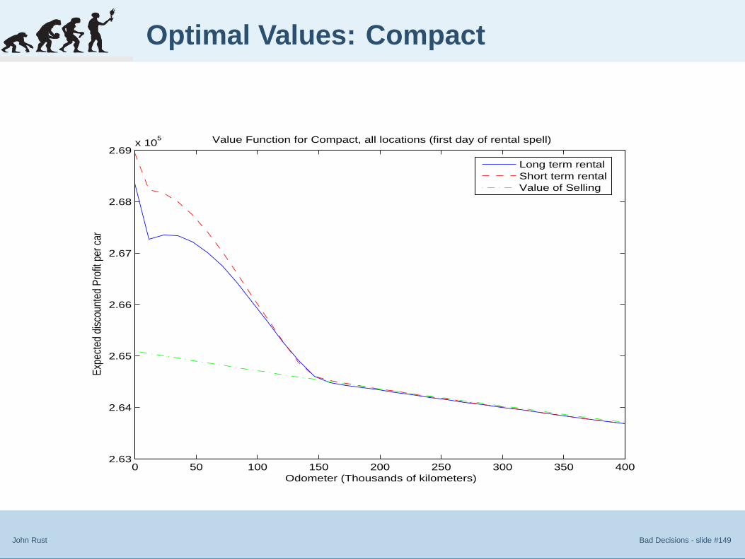
John Rust Bad Decisions - slide #149
Optimal Values: Compact
0 50 100 150 200 250 300 350 4002.63
2.64
2.65
2.66
2.67
2.68
2.69x 10
5
Odometer (Thousands of kilometers)
Expe
cted
disc
ount
ed P
rofit
per
car
Value Function for Compact, all locations (first day of rental spell)
Long term rentalShort term rentalValue of Selling
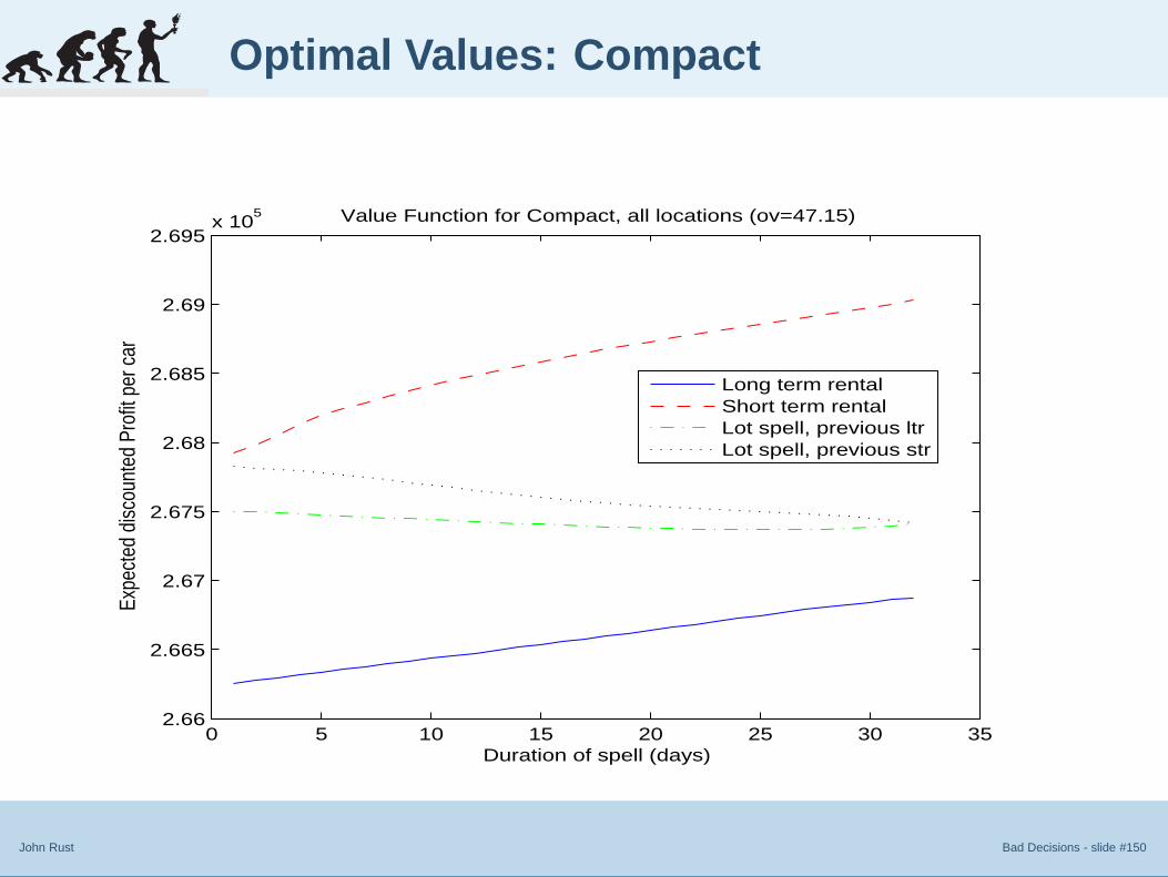
John Rust Bad Decisions - slide #150
Optimal Values: Compact
0 5 10 15 20 25 30 352.66
2.665
2.67
2.675
2.68
2.685
2.69
2.695x 10
5
Duration of spell (days)
Expe
cted
disc
ount
ed P
rofit
per
car
Value Function for Compact, all locations (ov=47.15)
Long term rentalShort term rentalLot spell, previous ltrLot spell, previous str

John Rust Bad Decisions - slide #151
Expected Revenue: Compact
0 5 10 15 20 25 30 35−200
0
200
400
600
800
1000
1200
1400
Duration of rental spell (days)
Expe
cted
dai
ly pr
ofit
per c
ar
Expected Rental Revenues given Rental Duration for Compact, all locations
Long term rentalShort term rental
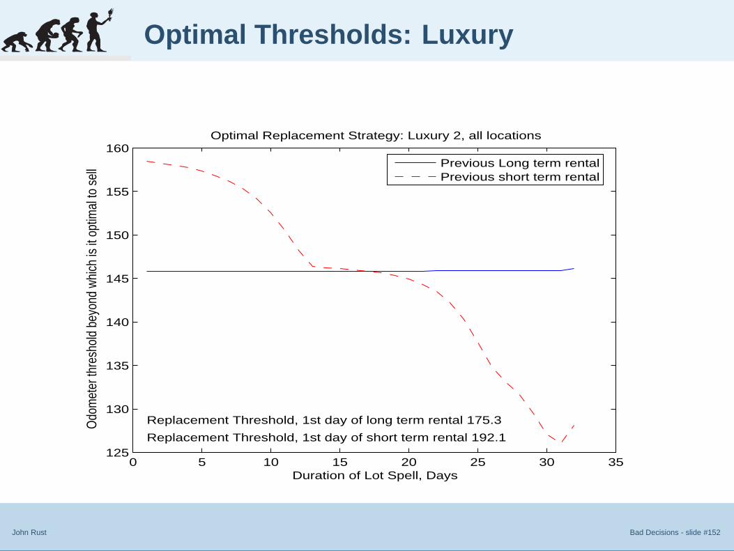
John Rust Bad Decisions - slide #152
Optimal Thresholds: Luxury
0 5 10 15 20 25 30 35125
130
135
140
145
150
155
160
Duration of Lot Spell, Days
Odo
met
er th
resh
old
beyo
nd w
hich
is it
opt
imal
to s
ell
Optimal Replacement Strategy: Luxury 2, all locations
Replacement Threshold, 1st day of long term rental 175.3
Replacement Threshold, 1st day of short term rental 192.1
Previous Long term rentalPrevious short term rental

John Rust Bad Decisions - slide #153
Optimal Values: Luxury
0 50 100 150 200 250 300 350 4003.56
3.58
3.6
3.62
3.64
3.66
3.68
3.7
3.72
3.74
3.76x 10
5
Odometer (Thousands of kilometers)
Expe
cted
disc
ount
ed P
rofit
per
car
Value Function for Luxury 2, all locations (first day of rental spell)
Long term rentalShort term rentalValue of Selling

John Rust Bad Decisions - slide #154
Optimal Values: Luxury
0 5 10 15 20 25 30 353.685
3.69
3.695
3.7
3.705
3.71
3.715x 10
5
Duration of spell (days)
Expe
cted
disc
ount
ed P
rofit
per
car
Value Function for Luxury 2, all locations (ov=47.15)
Long term rentalShort term rentalLot spell, previous ltrLot spell, previous str

John Rust Bad Decisions - slide #155
Expected Revenue: Luxury
0 5 10 15 20 25 30 35−500
0
500
1000
1500
2000
2500
Duration of rental spell (days)
Expe
cted
dai
ly pr
ofit
per c
ar
Expected Rental Revenues given Rental Duration for Luxury 2, all locations
Long term rentalShort term rental


John Rust Bad Decisions - slide #157
Optimal Thresholds: RV
0 5 10 15 20 25 30 35145
150
155
160
165
170
175
180
185
Duration of Lot Spell, Days
Odo
met
er th
resh
old
beyo
nd w
hich
is it
opt
imal
to s
ell
Optimal Replacement Strategy: RV, all locations
Replacement Threshold, 1st day of long term rental 170.6Replacement Threshold, 1st day of short term rental 202.5
Previous Long term rentalPrevious short term rental

John Rust Bad Decisions - slide #158
Optimal Values: RV
0 50 100 150 200 250 300 350 4003.14
3.16
3.18
3.2
3.22
3.24
3.26
3.28x 10
5
Odometer (Thousands of kilometers)
Expe
cted
disc
ount
ed P
rofit
per
car
Value Function for RV, all locations (first day of rental spell)
Long term rentalShort term rentalValue of Selling
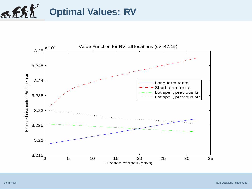
John Rust Bad Decisions - slide #159
Optimal Values: RV
0 5 10 15 20 25 30 353.215
3.22
3.225
3.23
3.235
3.24
3.245
3.25x 10
5
Duration of spell (days)
Expe
cted
disc
ount
ed P
rofit
per
car
Value Function for RV, all locations (ov=47.15)
Long term rentalShort term rentalLot spell, previous ltrLot spell, previous str
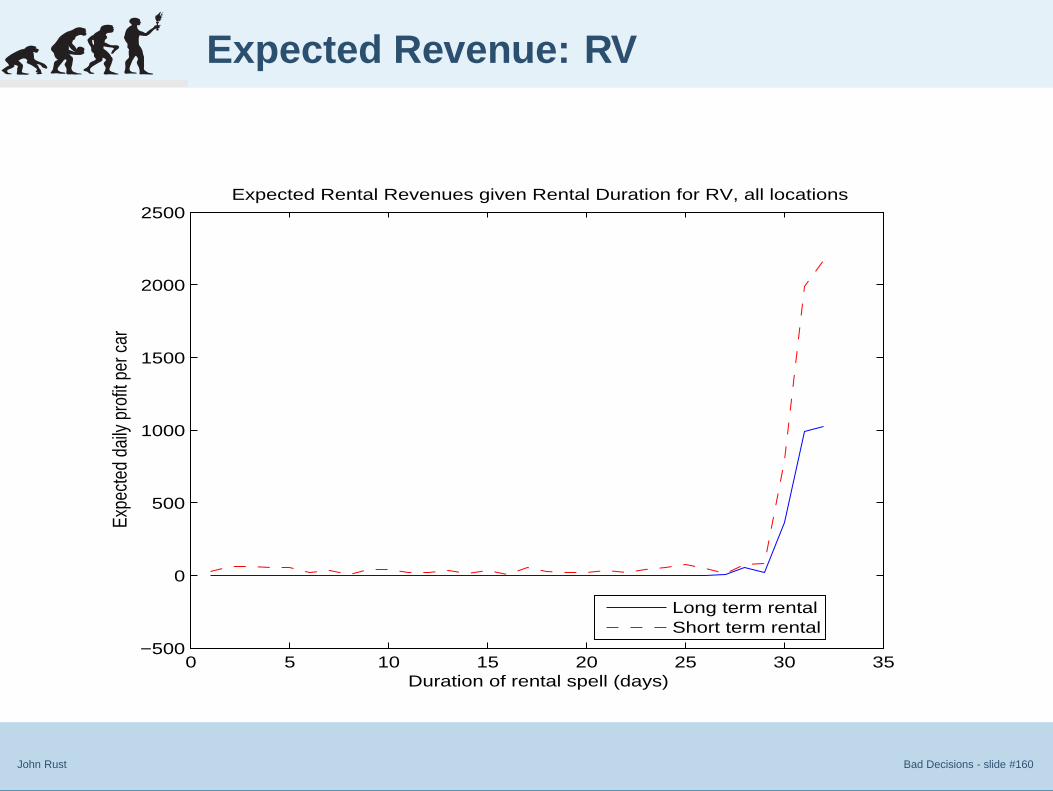
John Rust Bad Decisions - slide #160
Expected Revenue: RV
0 5 10 15 20 25 30 35−500
0
500
1000
1500
2000
2500
Duration of rental spell (days)
Expe
cted
dai
ly pr
ofit
per c
ar
Expected Rental Revenues given Rental Duration for RV, all locations
Long term rentalShort term rental


John Rust Bad Decisions - slide #162
Profit Comparisons
Quantity Compact Luxury RV
P 9668 23389 18774
Expected Discounted Values Under Optimal Replacement Policy
V (0, 0, r0) 268963 374913 327057
(1 − β)V (0, 0, r0) 22.11 30.81 26.88
V (0, 0, r0)/P 27.8 16.0 17.4
Expected Discounted Values Under Status Quo Replacement Policy
Vµ(0, 0, r0) 196589 318247 136792
(1 − β)Vµ(0, 0, r0) 16.16 26.16 11.24
V (0, 0, r0)µ/P 20.3 13.6 7.3
Ratio of Expected Values: Optimal Policy versus Status Quo
V (0, 0, r0)/Vµ(0, 0, r0) 1.37 1.18 2.39


Improving Disability
Determinations
Improving Return to Work
Incentives
Improving Car Rental Profits
6.5 Assessing Robustness
● Even More Pessimistic Case
● Maintenance Factors
● Rental Factors
● Profit Comparison
● Unanswered Questions
● Unanswered Questions, 2
● Unanswered Questions, 3
● Vehicle Portfolio Management
● Maximize Value or Return?
● Other Portfolio Consideration
● Data Requirements
● Rental Rate Structures
● Toward a Complete Model
● Future Directions
John Rust Bad Decisions - slide #164
Even More Pessimistic Case
1. To assess the robustness of our conclusions, we solved forthe optimal replacement policy under even more pessimisticassumptions about maintenance costs and the rentaldiscounts that would be required to induce customers torent older cars.
2. Under this more pessimistic scenario, maintenance costsstart to accelerate far earlier, at 60,000 kilometers.
3. We assume that rental rates start decreasing at a linearafter 60,000 kilometers until they hit zero at 210,000kilometers.
4. Even under this even more pessimistic scenario, the optimalreplacement policy still entails keeping cars about twice aslong (in terms of age or odometer value) as the companycurrently keeps them.

John Rust Bad Decisions - slide #165
Maintenance Factors
0 50 100 150 200 250 300 350 4000
1
2
3
4
5
6
7
8
9
10
11Assumed Multiplication Factor for Daily Maintenance Costs
Odometer (000 kilometers)
Mul
tiplic
atio
n F
acto
r
Scenario 1Scenario 2

John Rust Bad Decisions - slide #166
Rental Factors
0 50 100 150 200 250 300 350 4000
0.2
0.4
0.6
0.8
1
Assumed Multiplication Factor for Daily Rental Rates
Odometer (000 kilometers)
Mul
tiplic
atio
n F
acto
r
Scenario 1Scenario 2
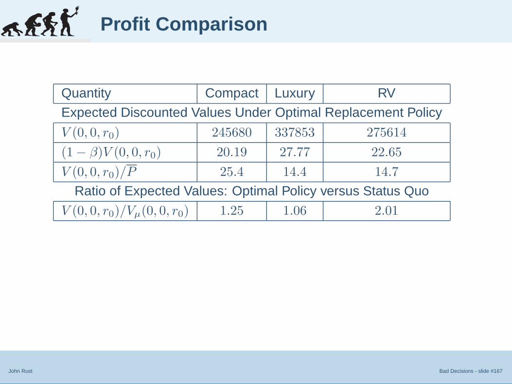
John Rust Bad Decisions - slide #167
Profit Comparison
Quantity Compact Luxury RV
Expected Discounted Values Under Optimal Replacement Policy
V (0, 0, r0) 245680 337853 275614
(1 − β)V (0, 0, r0) 20.19 27.77 22.65
V (0, 0, r0)/P 25.4 14.4 14.7
Ratio of Expected Values: Optimal Policy versus Status Quo
V (0, 0, r0)/Vµ(0, 0, r0) 1.25 1.06 2.01
Improving Disability
Determinations
Improving Return to Work
Incentives
Improving Car Rental Profits
6.5 Assessing Robustness
● Even More Pessimistic Case
● Maintenance Factors
● Rental Factors
● Profit Comparison
● Unanswered Questions
● Unanswered Questions, 2
● Unanswered Questions, 3
● Vehicle Portfolio Management
● Maximize Value or Return?
● Other Portfolio Consideration
● Data Requirements
● Rental Rate Structures
● Toward a Complete Model
● Future Directions
John Rust Bad Decisions - slide #168
Unanswered Questions
■ Our analysis has been focused mainly on the narrowquestion of the timing of replacement decisions,
■ We believe we have provided convincing evidence that viamodest changes in the company’s operating strategy, it cansignificantly increase discounted profits.
■ However our analysis leaves a number of unansweredquestions:

Improving Disability
Determinations
Improving Return to Work
Incentives
Improving Car Rental Profits
6.5 Assessing Robustness
● Even More Pessimistic Case
● Maintenance Factors
● Rental Factors
● Profit Comparison
● Unanswered Questions
● Unanswered Questions, 2
● Unanswered Questions, 3
● Vehicle Portfolio Management
● Maximize Value or Return?
● Other Portfolio Consideration
● Data Requirements
● Rental Rate Structures
● Toward a Complete Model
● Future Directions
John Rust Bad Decisions - slide #168
Unanswered Questions
■ Our analysis has been focused mainly on the narrowquestion of the timing of replacement decisions,
■ We believe we have provided convincing evidence that viamodest changes in the company’s operating strategy, it cansignificantly increase discounted profits.
■ However our analysis leaves a number of unansweredquestions:1. Given how successful this company is at what it does,
how could it fail to recognize the benefits from keeping itsvehicles longer?
2. Are there any overlooked considerations, constraints, orregulations that might explain why the company decidesto replace its rental vehicles “too frequently”?

Improving Disability
Determinations
Improving Return to Work
Incentives
Improving Car Rental Profits
6.5 Assessing Robustness
● Even More Pessimistic Case
● Maintenance Factors
● Rental Factors
● Profit Comparison
● Unanswered Questions
● Unanswered Questions, 2
● Unanswered Questions, 3
● Vehicle Portfolio Management
● Maximize Value or Return?
● Other Portfolio Consideration
● Data Requirements
● Rental Rate Structures
● Toward a Complete Model
● Future Directions
John Rust Bad Decisions - slide #169
Unanswered Questions, 2
■ Our analysis of sales prices revealed very large variations inthe price received for apparently “observationally equivalent”vehicles.

Improving Disability
Determinations
Improving Return to Work
Incentives
Improving Car Rental Profits
6.5 Assessing Robustness
● Even More Pessimistic Case
● Maintenance Factors
● Rental Factors
● Profit Comparison
● Unanswered Questions
● Unanswered Questions, 2
● Unanswered Questions, 3
● Vehicle Portfolio Management
● Maximize Value or Return?
● Other Portfolio Consideration
● Data Requirements
● Rental Rate Structures
● Toward a Complete Model
● Future Directions
John Rust Bad Decisions - slide #169
Unanswered Questions, 2
■ Our analysis of sales prices revealed very large variations inthe price received for apparently “observationally equivalent”vehicles.1. Why would the company “precommitt” to selling a vehicle
on a particular date for the best price offered on that date,even if the best price seems below the fair market valuefor the vehicle?
Improving Disability
Determinations
Improving Return to Work
Incentives
Improving Car Rental Profits
6.5 Assessing Robustness
● Even More Pessimistic Case
● Maintenance Factors
● Rental Factors
● Profit Comparison
● Unanswered Questions
● Unanswered Questions, 2
● Unanswered Questions, 3
● Vehicle Portfolio Management
● Maximize Value or Return?
● Other Portfolio Consideration
● Data Requirements
● Rental Rate Structures
● Toward a Complete Model
● Future Directions
John Rust Bad Decisions - slide #170
Unanswered Questions, 3
■ Our analysis of the relative profitability of long and short termrental contracts revealed that for some vehicles, such as thecompact car, short term contracts are significantly moreprofitable than long term contracts.
Improving Disability
Determinations
Improving Return to Work
Incentives
Improving Car Rental Profits
6.5 Assessing Robustness
● Even More Pessimistic Case
● Maintenance Factors
● Rental Factors
● Profit Comparison
● Unanswered Questions
● Unanswered Questions, 2
● Unanswered Questions, 3
● Vehicle Portfolio Management
● Maximize Value or Return?
● Other Portfolio Consideration
● Data Requirements
● Rental Rate Structures
● Toward a Complete Model
● Future Directions
John Rust Bad Decisions - slide #170
Unanswered Questions, 3
■ Our analysis of the relative profitability of long and short termrental contracts revealed that for some vehicles, such as thecompact car, short term contracts are significantly moreprofitable than long term contracts.1. Why doesn’t the company adjust the rental rates to
equalize the relative profitability of long and short termcontracts?
■ Our analysis also revealed big differences in the overallprofitability of different vehicles. In particular, the stream ofdiscounted profits from rental of the RV or luxury car typesare 20 and 40% higher, respectively.

Improving Disability
Determinations
Improving Return to Work
Incentives
Improving Car Rental Profits
6.5 Assessing Robustness
● Even More Pessimistic Case
● Maintenance Factors
● Rental Factors
● Profit Comparison
● Unanswered Questions
● Unanswered Questions, 2
● Unanswered Questions, 3
● Vehicle Portfolio Management
● Maximize Value or Return?
● Other Portfolio Consideration
● Data Requirements
● Rental Rate Structures
● Toward a Complete Model
● Future Directions
John Rust Bad Decisions - slide #170
Unanswered Questions, 3
■ Our analysis of the relative profitability of long and short termrental contracts revealed that for some vehicles, such as thecompact car, short term contracts are significantly moreprofitable than long term contracts.1. Why doesn’t the company adjust the rental rates to
equalize the relative profitability of long and short termcontracts?
■ Our analysis also revealed big differences in the overallprofitability of different vehicles. In particular, the stream ofdiscounted profits from rental of the RV or luxury car typesare 20 and 40% higher, respectively.1. If these vehicles are so much more profitable, why not
allocate more lot space on the margin to luxury and RVs,or alternatively, increase rental rates on compact cars toincrease their relatively profitability?

Improving Disability
Determinations
Improving Return to Work
Incentives
Improving Car Rental Profits
6.5 Assessing Robustness
● Even More Pessimistic Case
● Maintenance Factors
● Rental Factors
● Profit Comparison
● Unanswered Questions
● Unanswered Questions, 2
● Unanswered Questions, 3
● Vehicle Portfolio Management
● Maximize Value or Return?
● Other Portfolio Consideration
● Data Requirements
● Rental Rate Structures
● Toward a Complete Model
● Future Directions
John Rust Bad Decisions - slide #171
Vehicle Portfolio Management
■ Economists are accustomed to “marginal arguments” foroptimal decision making.
■ The rental company must select a “portfolio” of vehicles forthe lots in each of its rental locations.
■ Similar to standard portfolio analysis in finance, at an optimalallocation the company should be getting roughly the sameexpected “risk adjusted return” from an investment of $X incar type τ1 as it does for an equivalent investment in car typeτ2.
■ Otherwise if there is one type of car that has a higher returnper dollar invested, then the firm would be better off investingthe marginal dollar in the car type that yields the highestpossible returns.
■ Our analysis has revealed that of the three car types we haveanalyzed, the compact has the highest rate of return eventhough it has the lowest discounted value of profits per car.

Improving Disability
Determinations
Improving Return to Work
Incentives
Improving Car Rental Profits
6.5 Assessing Robustness
● Even More Pessimistic Case
● Maintenance Factors
● Rental Factors
● Profit Comparison
● Unanswered Questions
● Unanswered Questions, 2
● Unanswered Questions, 3
● Vehicle Portfolio Management
● Maximize Value or Return?
● Other Portfolio Consideration
● Data Requirements
● Rental Rate Structures
● Toward a Complete Model
● Future Directions
John Rust Bad Decisions - slide #172
Maximize Value or Return?
■ It is not completely obvious that the correct way to thinkabout the firm’s allocation problem as choosing to invest inthe car with the high marginal return, or to allocate cars to afixed level of lot space to maximize the overall value ofdiscounted profits.
■ These two criterion for the portfolio management problemseem to result in different allocations, at least on the margin.
■ That is, if the company wants to get the highest return on itsinvestment, it would appear it should allocate more of itsvehicle “portfolio” to compacts and less to luxury or RVs.
■ However if it is interested in maximizing the expected presentvalue of profits, then it would appear that it should allocatemore of its vehicle portfolio to the luxury and RV car types.

Improving Disability
Determinations
Improving Return to Work
Incentives
Improving Car Rental Profits
6.5 Assessing Robustness
● Even More Pessimistic Case
● Maintenance Factors
● Rental Factors
● Profit Comparison
● Unanswered Questions
● Unanswered Questions, 2
● Unanswered Questions, 3
● Vehicle Portfolio Management
● Maximize Value or Return?
● Other Portfolio Consideration
● Data Requirements
● Rental Rate Structures
● Toward a Complete Model
● Future Directions
John Rust Bad Decisions - slide #173
Other Portfolio Consideration
■ There could be complimentarities between cars of differenttypes, and the firm should try to cater to its customers’preferences.
■ Clearly some customers will want to rent compacts, otherswill prefer RVs and others will prefer to have luxury vehicles.
■ If the company happens to be “stocked out” of a particularcustomer’s most preferred type of vehicle, having a portfoliowith sufficiently close substitutes may enable the company tokeep that customer, as opposed to the customer walkingdown to the next rental company window to see if acompetitor has their preferred vehicle in stock and ready torent.

Improving Disability
Determinations
Improving Return to Work
Incentives
Improving Car Rental Profits
6.5 Assessing Robustness
● Even More Pessimistic Case
● Maintenance Factors
● Rental Factors
● Profit Comparison
● Unanswered Questions
● Unanswered Questions, 2
● Unanswered Questions, 3
● Vehicle Portfolio Management
● Maximize Value or Return?
● Other Portfolio Consideration
● Data Requirements
● Rental Rate Structures
● Toward a Complete Model
● Future Directions
John Rust Bad Decisions - slide #174
Data Requirements
■ Our data do not include information on customers, theirarrival rates to various rental locations and driving/returnpatterns (i.e. the probability that a car rented at location Awill actually be returned to location B).
■ Without more data on customer choices, and data on thecompany’s competitors, it is difficult for us to formulate amore comprehensive model of the overall operations of thiscompany.
■ However we believe the analysis we have conducted in thispaper constitutes a fundamental “building block” toward amore complete analysis of this optimal (i.e. profitmaximizing) operation of this company.
■ Whatever portfolio allocation of rental vehicles, and rentalrates the company chooses, it will want to adopt a vehiclereplacement policy that is optimal conditional on its vehicleportfolio and rental rate structure.

Improving Disability
Determinations
Improving Return to Work
Incentives
Improving Car Rental Profits
6.5 Assessing Robustness
● Even More Pessimistic Case
● Maintenance Factors
● Rental Factors
● Profit Comparison
● Unanswered Questions
● Unanswered Questions, 2
● Unanswered Questions, 3
● Vehicle Portfolio Management
● Maximize Value or Return?
● Other Portfolio Consideration
● Data Requirements
● Rental Rate Structures
● Toward a Complete Model
● Future Directions
John Rust Bad Decisions - slide #175
Rental Rate Structures
■ Let Mi be the maximum number of cars that the firm hasavailable in location i, i = 1, . . . , N .
■ Suppose there are J possible car types (i.e. individualmakes and models of cars), and the firm has adopted arental rate structure R.
■ Initially we adopt the simplication that a rental rate plan forcar type j at location i consists of two numbers {(Rl
ij , Rsij)}
representing flat daily rental rates for long and short termrentals for each car type j at rental location i.
■ Thus a rental rate structure consists of the complete array ofall rental prices at all rental locations,R = {(Rl
ij , Rsij), j = 1, . . . , J, i = 1, . . . , N}.
■ Rental rate structures are more complicated if we allowcontracts with odometer-based discounts, and usage-basedrental schemes.
Improving Disability
Determinations
Improving Return to Work
Incentives
Improving Car Rental Profits
6.5 Assessing Robustness
● Even More Pessimistic Case
● Maintenance Factors
● Rental Factors
● Profit Comparison
● Unanswered Questions
● Unanswered Questions, 2
● Unanswered Questions, 3
● Vehicle Portfolio Management
● Maximize Value or Return?
● Other Portfolio Consideration
● Data Requirements
● Rental Rate Structures
● Toward a Complete Model
● Future Directions
John Rust Bad Decisions - slide #176
Toward a Complete Model
■ Let Vij(R) denote the expected discounted value of profitsfrom a car of type j in rental location i under the assumptiontha the firm follows an optimal replacement strategy for eachcar type j at each location i under rental rate structure R.
■ Let P j be the new purchase price of car type j.

Improving Disability
Determinations
Improving Return to Work
Incentives
Improving Car Rental Profits
6.5 Assessing Robustness
● Even More Pessimistic Case
● Maintenance Factors
● Rental Factors
● Profit Comparison
● Unanswered Questions
● Unanswered Questions, 2
● Unanswered Questions, 3
● Vehicle Portfolio Management
● Maximize Value or Return?
● Other Portfolio Consideration
● Data Requirements
● Rental Rate Structures
● Toward a Complete Model
● Future Directions
John Rust Bad Decisions - slide #176
Toward a Complete Model
■ Let Vij(R) denote the expected discounted value of profitsfrom a car of type j in rental location i under the assumptiontha the firm follows an optimal replacement strategy for eachcar type j at each location i under rental rate structure R.
■ Let P j be the new purchase price of car type j.■ Then we can formulate the overall optimal rental operations
problem as the following programming problem
maxR
max{Nij}
N∑i=1
J∑j=1
Nij [Vij(R)−P j ] subject to:J∑
j=1
Nij ≤ Mi(11)
■ Nested within this problem is the regnerative optimalstopping problem, that we have solved in this paper, thatdelivers the value function Vij(R) for all car types at all of thefirm’s rental locations.

Improving Disability
Determinations
Improving Return to Work
Incentives
Improving Car Rental Profits
6.5 Assessing Robustness
● Even More Pessimistic Case
● Maintenance Factors
● Rental Factors
● Profit Comparison
● Unanswered Questions
● Unanswered Questions, 2
● Unanswered Questions, 3
● Vehicle Portfolio Management
● Maximize Value or Return?
● Other Portfolio Consideration
● Data Requirements
● Rental Rate Structures
● Toward a Complete Model
● Future Directions
John Rust Bad Decisions - slide #177
Future Directions
■ With better data on all of the company’s rental locations andcustomer data, it may be possible to solve this programmingproblem.
■ We also need to recognize that the optimal choice of a rentalrate structure depends on the choices Rc of the company’scompetitors, c ∈ C.
■ In this larger competitive game, the firm’s value and theoptimal strategy for its vehicle portfolio and rental ratestructure will clearly depend on the portfolios and rental ratestructures chosen by its competitors.
■ Solving for the overall competitive equilibrium problem in therental market remains a challenging area for future research.


John Rust Bad Decisions - slide #179
Saddam in happier times
(shown after receiving billions in U.S. arms from Donald Rumsfeld)

John Rust Bad Decisions - slide #180
George Bush, compassionate conservative