Backtracking search: look-back

Chapter 6

Look-back: Backjumping / Learning

Backjumping: • In deadends, go back to

the most recent culprit.

Learning: • constraint-recording, no-

good recording.

• good-recording

Backjumping

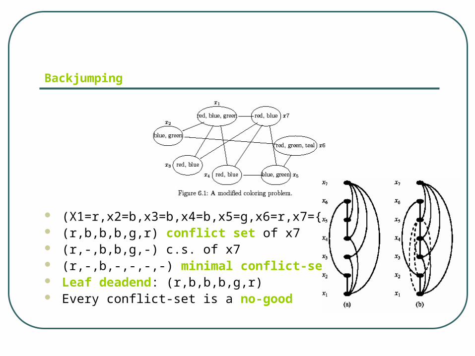
(X1=r,x2=b,x3=b,x4=b,x5=g,x6=r,x7={r,b}) (r,b,b,b,g,r) conflict set of x7 (r,-,b,b,g,-) c.s. of x7 (r,-,b,-,-,-,-) minimal conflict-set Leaf deadend: (r,b,b,b,g,r) Every conflict-set is a no-good

Gaschnig jumps only at leaf-dead-endsInternal dead-ends: dead-ends that are non-leaf

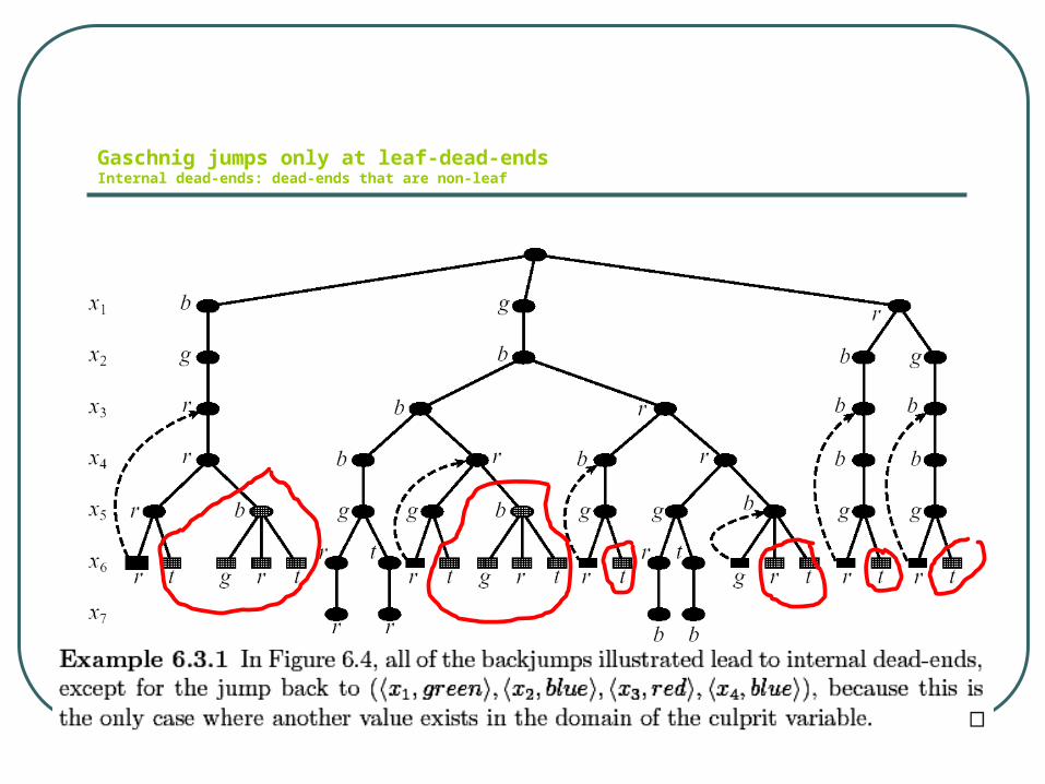
Gaschnig jumps only at leaf-dead-endsInternal dead-ends: dead-ends that are non-leaf

Backjumping styles

Jump at leaf only (Gaschnig 1977)• Context-based

Graph-based (Dechter, 1990)• Jumps at leaf and internal dead-ends

Conflict-directed (Prosser 1993)• Context-based, jumps at leaf and internal dead-ends

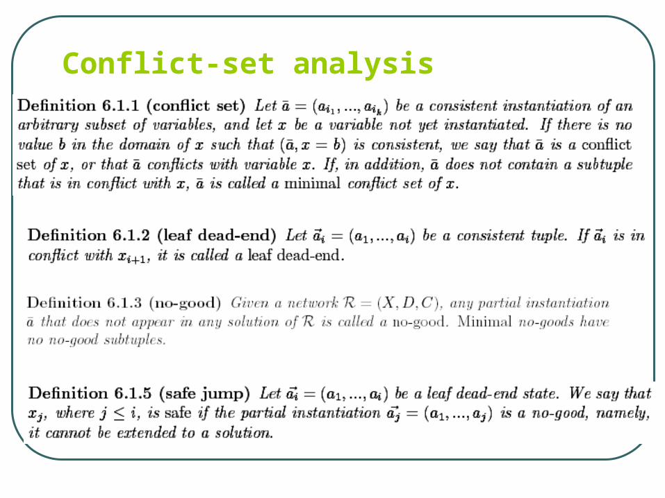
Conflict-set analysis

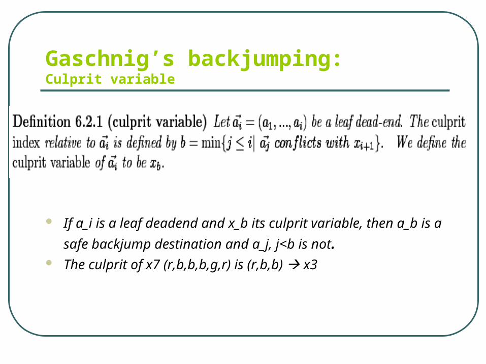
Gaschnig’s backjumping:Culprit variable

If a_i is a leaf deadend and x_b its culprit variable, then a_b is a

safe backjump destination and a_j, j<b is not. The culprit of x7 (r,b,b,b,g,r) is (r,b,b) x3

Gaschnig’s backjumping [1979]

Gaschnig uses a marking technique to compute the culprit.

Each variable xj maintains a pointer (latset_j) to the latest ancestor incompatible with any of its values.

While forward generating , keep array latest_i, 1<=j<=n, of pointers to the last value conflicted with some value of x_j

The algorithm jumps from a leaf-dead-end x_{i+1} back to latest_(i+1) which is its culprit.

ia

Gaschnig’s backjumping

Example of Gaschnig’s backjump

Properties

Gaschnig’s backjumping implements only safe and maximal backjumps in leaf-deadends.

Gaschnig jumps only at leaf-dead-endsInternal dead-ends: dead-ends that are non-leaf

Graph-based backjumping scenarios

Scenario 1, deadend at x4: Scenario 2: deadend at x5: Scenario 3: deadend at x7: Scenario 4: deadend at x6: },{),,(

},{),,(

}{),(

}{)(

314564

314574

1544

144

xxxxxI

xxxxxI

xxxI

xxI

Graph-based backjumping

Uses only graph information to find culprit Jumps both at leaf and at internal dead-ends Whenever a deadend occurs at x, it jumps to the most

recent variable y connected to x in the graph. If y is an internal deadend it jumps back further to the most recent variable connected to x or y.

The analysis of conflict is approximated by the graph. Graph-based algorithm provide graph-theoretic bounds.

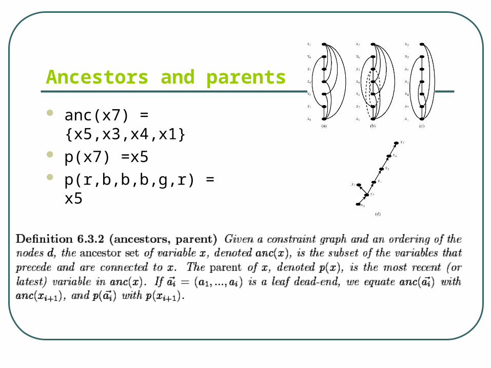
Ancestors and parents

anc(x7) = {x5,x3,x4,x1} p(x7) =x5 p(r,b,b,b,g,r) = x5

Internal deadends analysis

Graph-based backjumping algorithm,but we need to jump at internal deadends too

Properties of graph-based backjumping

Algorithm graph-based backjumping jumps back at any deadend variable as far as graph-based information allows.

For each variable, the algorithm maintains the induced-ancestor set I_i relative the relevant dead-ends in its current session.

The size of the induced ancestor set is at most w*(d).

Conflict-directed backjumping(Prosser 1990)

Extend Gaschnig’s backjump to internal dead-ends. Exploits information gathered during search. For each variable the algorithm maintains an induced

jumpback set, and jumps to most recent one. Use the following concepts:

• An ordering over variales induced a strict ordering between constraints: R1<R2<…Rt

• Use earliest minimal consflict-set (emc(x_(i+1)) ) of a deadend.

• Define the jumpback set of a deadend

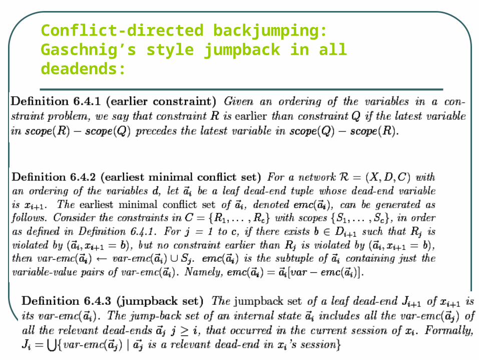
Conflict-directed backjumping:Gaschnig’s style jumpback in all deadends:

Example of conflict-directed backjumping

Properties

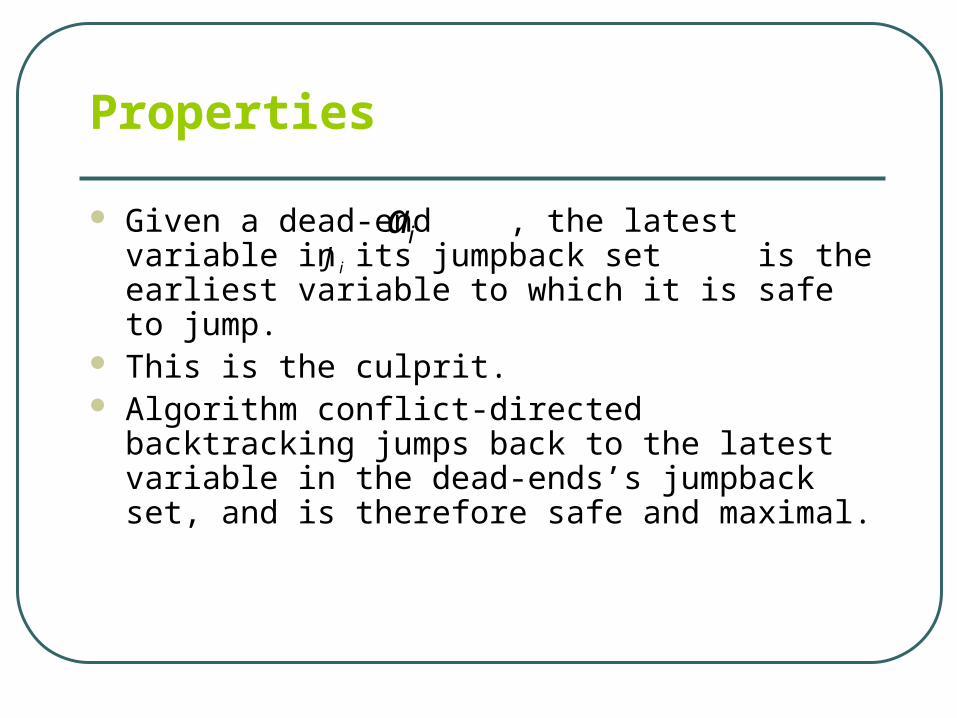
Given a dead-end , the latest variable in its jumpback set is the earliest variable to which it is safe to jump.

This is the culprit. Algorithm conflict-directed backtracking jumps back

to the latest variable in the dead-ends’s jumpback set, and is therefore safe and maximal.

ia

iJ

Conflict-directed backjumping

Graph-based backjumping on DFS orderings

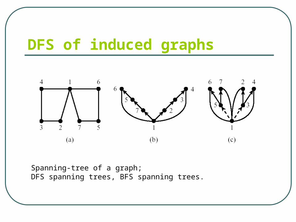
DFS of induced graphs

Spanning-tree of a graph;DFS spanning trees, BFS spanning trees.

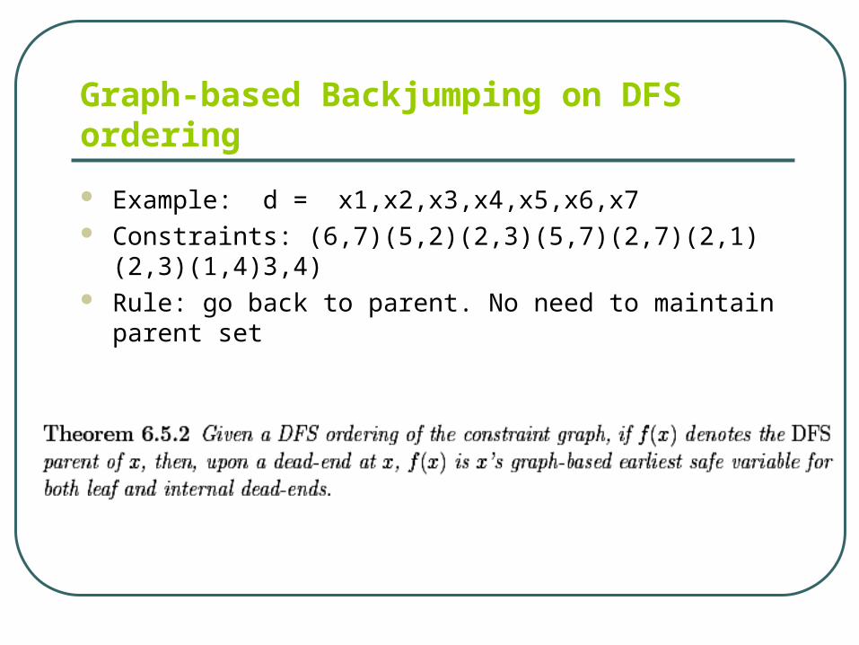
Graph-based Backjumping on DFS ordering

Example: d = x1,x2,x3,x4,x5,x6,x7 Constraints: (6,7)(5,2)(2,3)(5,7)(2,7)(2,1)(2,3)(1,4)3,4) Rule: go back to parent. No need to maintain parent set

Complexity of Graph-based Backjumping

T_i= number of nodes in the AND/OR search space rooted at x_i (level m-i)

Each assignment of a value to x_i generates subproblems:

• T_i = k b T_{i-1}

• T_0 = k Solution:

1 mmm kbT

Complexity (continued)

A better bound: The AND/OR search space is bound by O(n) regular searches of at most m variables yielding O(n k^m) nodes.

DFS of induced graphs

Complexity of Backjumpinguses pseudo-tree analysis

Simple: always jump back to parent in pseudo treeComplexity for csp: exp(tree-depth)Complexity for csp: exp(w*log n)

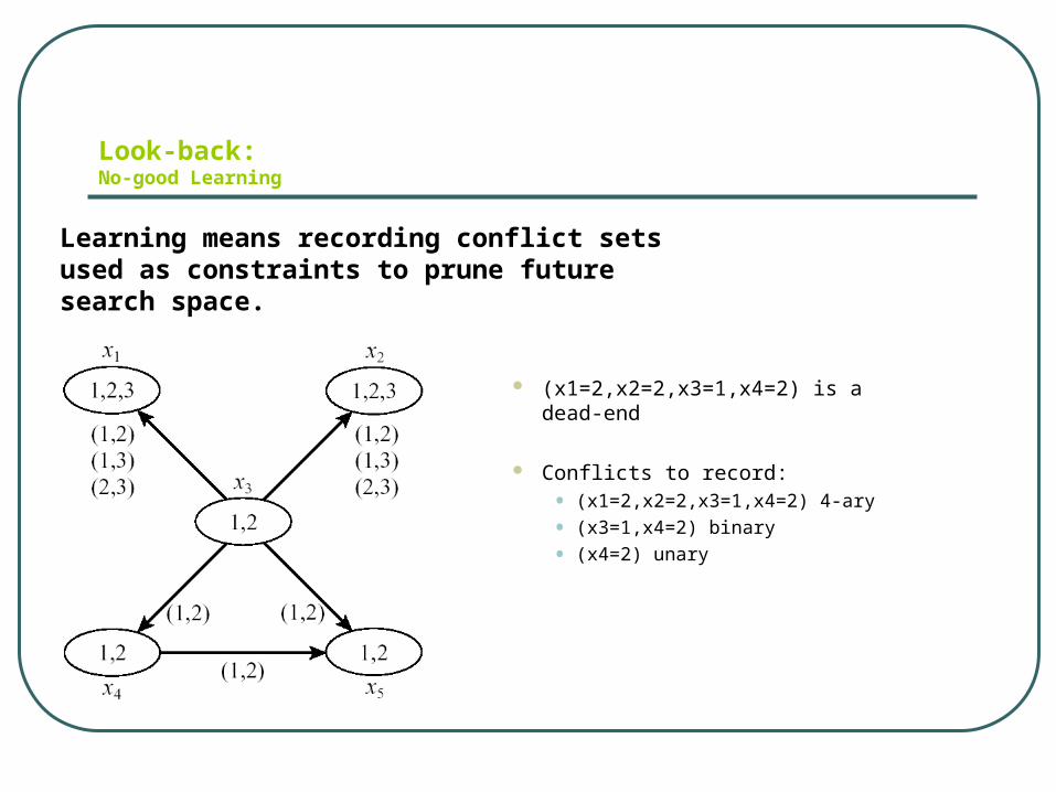
Look-back: No-good Learning

(x1=2,x2=2,x3=1,x4=2) is a dead-end

Conflicts to record:

• (x1=2,x2=2,x3=1,x4=2) 4-ary

• (x3=1,x4=2) binary

• (x4=2) unary

Learning means recording conflict setsused as constraints to prune future search space.

Learning, constraint recording

Learning means recording conflict sets An opportunity to learn is when deadend is

discovered. Goal of learning to not discover the same deadends. Try to identify small conflict sets Learning prunes the search space.

Learning example

Learning Issues

Learning styles• Graph-based or context-based

• i-bounded, scope-bounded

• Relevance-based

Non-systematic randomized learning Implies time and space overhead Applicable to SAT

Graph-based learning algorithm

Deep learning

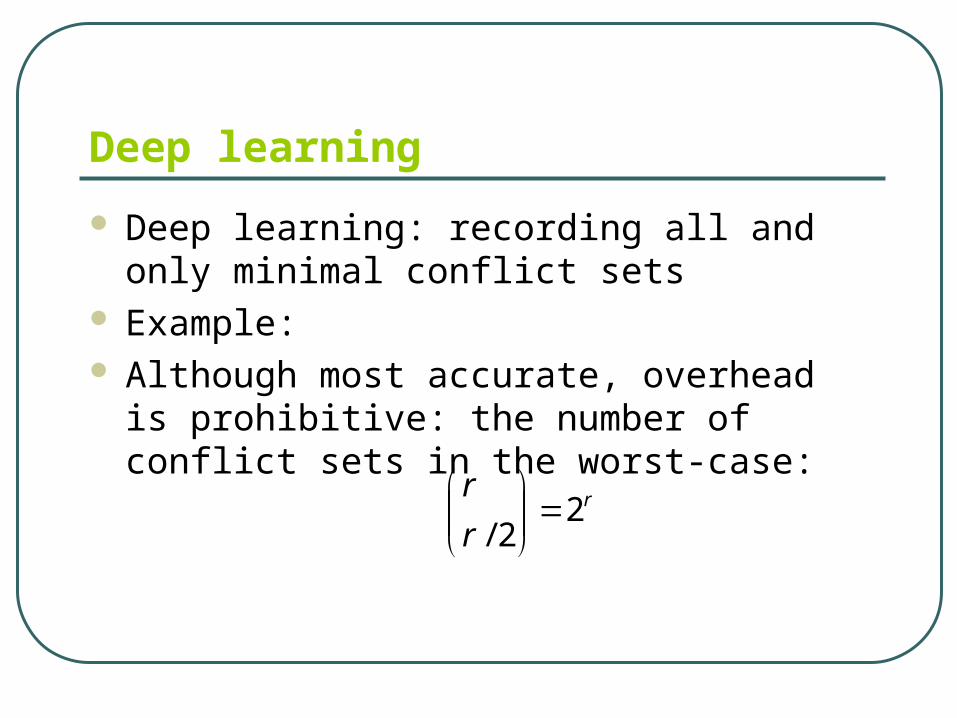
Deep learning: recording all and only minimal conflict sets

Example: Although most accurate, overhead is

prohibitive: the number of conflict sets in the worst-case:

r

r

r2

2/

Jumpback Learning

Record the jumpback assignment

Bounded and relevance-based learning Bounding the arity of constraints recorded. When bound is i: i-ordered graph-based,i-order jumpback or

i-order deep learning. Overhead complexity of i-bounded learning is time and

space exponential in i.

Complexity of backtrack-learning

The number of dead-ends is bounded by the number of possible no-goods of size w* or less

Number of constraint tests per dead-end are

))(( 1)()(

1

*

*

dwidw

i

nkOki

n

)2( )(* dwO

Complexity of backtrack-learning (improved)

Theorem: Any backtracking algorithm using graph-based learning along d has a space complexity O(n k^w*(d)) and time complexity O(n^2 (2k)^(w*(d)+1) (book). Refined more: O(n^2 k^w*(d))

Proof: The number of deadends for each variable is O(k^w*(d)), yielding O(n k^w*(d)) deadends.There are at most kn values between two succesive deadends: O(k n^2 k^w*(d)) number of nodes in the search space. Since at most O(2^w*(d)) constraints-checks we get O(n^2 (2k)^(w*(d)+1).

Improved more: If we have O(n k^w*(d)) leaves, we have k to n times as many internal nodes, yielding between O(n k^(w*(d)+1)) and O(n^2 k^w*(d)) nodes.

Backjumping and Learning on DFS?

Can we have a better bound than O(n^2 k^m*)? m*(d) <= log n w*(d) Therefore, to reduce time by a factor of k^(log n), we

need k^w*(d) space.

Complexity of Backtrack-Learningfor CSP

The number of dead-ends is bounded byNumber of constraint tests per dead-end are

Space complexity is Time complexity is )(

)()*(2

)*(

dw

dw

kenO

nkO

The complexity of learning along d is time and space exponential in w*(d):

)( )*(dwnkO)(eO

Complexity of Backtrack-Learningfor CSP

The number of dead-ends is bounded byNumber of constraint tests per dead-end are

Space complexity is Time complexity is Learning and backjumping: O(n m e k^w*(d))

)(

)()*(2

)*(

dw

dw

kenO

nkO

The complexity of learning along d is time and space exponential in w*(d):

)( )*(dwnkO)(eO

M- depth of tree, e- number of constraints

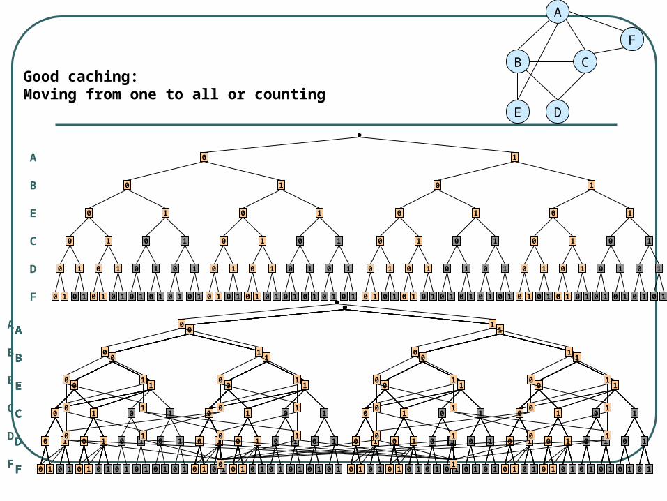
Good caching:Moving from one to all or counting

E 0 1 0 1 0 1 0 1

0C 1 0 1 0 1 0 1 0 1 0 1 0 1 0 1

F 0 1 0 1 0 1 0 1 0 1 0 1 0 1 0 1 0 1 0 1 0 1 0 1 0 1 0 1 0 1 0 1 0 1 0 1 0 1 0 1 0 1 0 1 0 1 0 1 0 1 0 1 0 1 0 1 0 1 0 1 0 1 0 1

D 0 1 0 1 0 1 0 1 0 1 0 1 0 1 0 1 0 1 0 1 0 1 0 1 0 1 0 1 0 1 0 1

0B 1 0 1

A 0 1

E 0 1 0 1 0 1 0 1

0C 1 0 1 0 1 0 1 0 1 0 1 0 1 0 1

F 0 1 0 1 0 1 0 1 0 1 0 1 0 1 0 1 0 1 0 1 0 1 0 1 0 1 0 1 0 1 0 1 0 1 0 1 0 1 0 1 0 1 0 1 0 1 0 1 0 1 0 1 0 1 0 1 0 1 0 1 0 1 0 1

D 0 1 0 1 0 1 0 1 0 1 0 1 0 1 0 1 0 1 0 1 0 1 0 1 0 1 0 1 0 1 0 1

0B 1 0 1

A 0 1

E 0 1 0 1 0 1 0 1

0C 1 0 1 0 1 0 1 0 1 0 1 0 1

F 0 1 0 1 0 1 0 1 0 1 0 1 0 1 0 1 0 1 0 1 0 1 0 1 0 1 0 1 0 1 0 1 0 1 0 1 0 1 0 1 0 1 0 1 0 1 0 1 0 1 0 1 0 1 0 1

D 0 1 0 1 0 1 0 1 0 1 0 1 0 1 0 1 0 1 0 1 0 1 0 1 0 1 0 1

0B 1 0 1

A 0 1

E 0 1 0 1 0 1 0 1

0C 1 0 1 0 1 0 1 0 1

F 0 1 0 1 0 1 0 1 0 1 0 1 0 1 0 1 0 1 0 1 0 1 0 1 0 1 0 1 0 1 0 1 0 1 0 1 0 1 0 1

D 0 1 0 1 0 1 0 1 0 1 0 1 0 1 0 1 0 1 0 1

0B 1 0 1

A 0 1

E 0 1 0 1 0 1 0 1

0C 1 0 1 0 1 0 1 0 1 0 1

F 0 1 0 1 0 1 0 1 0 1 0 1 0 1 0 1 0 1 0 1 0 1 0 1 0 1 0 1 0 1 0 1 0 1 0 1 0 1 0 1 0 1 0 1 0 1 0 1

D 0 1 0 1 0 1 0 1 0 1 0 1 0 1 0 1 0 1 0 1 0 1 0 1

0B 1 0 1

A 0 1

E 0 1 0 1 0 1 0 1

0C 1 0 1 0 1 0 1

F 0 1 0 1 0 1 0 1 0 1 0 1 0 1 0 1 0 1 0 1 0 1 0 1 0 1 0 1 0 1 0 1

D 0 1 0 1 0 1 0 1 0 1 0 1 0 1 0 1

0B 1 0 1

A 0 1

E 0 1 0 1 0 1 0 1

0C 1 0 1 0 1 0 1

F 0 1 0 1 0 1 0 1 0 1 0 1 0 1 0 1

D 0 1 0 1 0 1 0 1 0 1 0 1 0 1 0 1

0B 1 0 1

A 0 1

0 1 0 1 0 1 0 1

0 1 0 1 0 1 0 1

0 1

0 1 0 1

E

C

F

D

B

A 0 1

0 1

0 1 0 1 0 1

A

D

B C

E

F

Summary: time-space for constraint processing

Constraint-satisfaction• Search with backjumping

• Space: linear, Time: O(exp(logn w*))

• Search with learning no-goods• time and space: O(exp(w*))

• Variable-elimination• time and space: O(exp(w*))

Counting, enumeration• Search with backjumping

• Space: linear, Time: O(exp(n ))

• Search with no-goods caching only• space: O(exp(w*)) Time: O(exp(n))

• Search with goods and no-goods learning• Time and space: O(exp(path-width), O(exp(log n w*))

• Variable-elimination• Time and space: O(exp(w*))

Non-Systematic Randomized Learning

Do search in a random way with interupts, restarts, undafe backjumping, but record conflicts.

Guaranteed completeness.

Look-back for SAT

A partial assignment is a set of literals: A jumpback set if a J-clause: Upon a leaf deadend of xx resolve two clauses, one enforcing x

and one enforcing ~x relative to the current assignment A clause forces x relative to assignment if all the literals in

the clause are negated in . Resolving the two clauses we get a nogood. If we identify the earliest two clauses we will find the earliest

condlict. The argument can be extended to internal deadends.

Look-back for SAT

Integration of algorithms

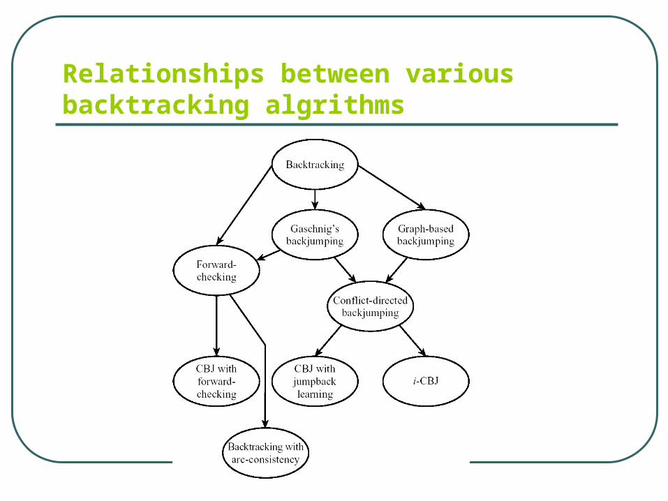
Relationships between various backtracking algrithms

Empirical comparison of algorithms

Benchmark instances Random problems Application-based random problems Generating fixed length random k-sat

(n,m) uniformly at random Generating fixed length random CSPs (N,K,T,C) also arity, r.

The Phase transition (m/n)

Some empirical evaluation Sets 1-3 reports average over 2000 instances of random

csps from 50% hardness. Set 1: 200 variables, set 2: 300, Set 3: 350. All had 3 values.:

Dimacs problems