background suppression through pulse shape analysis in the
TRANSCRIPT
Background Suppression through Pulse Shape Analysis in the
DEAP-3600 Dark Matter Detector
April 3, 2018
Master’s thesis submitted by
Paul Moritz Burghardt
Supervisor:
Dr. Tina Pollmann
First corrector:
Prof. Dr. Stefan Schonert
Department of Physics,
Technical University of Munich
Abstract
DEAP-3600 is a dark matter direct detection experiment in SNOLAB, Canada, using a single
phase liquid argon target. Upon energy deposition of ionising particles, liquid argon emits light
through the decay of a short-lived singlet state and a long-lived triplet state with a lifetime of
approx 1400 ns. In DEAP-3600 this makes up the only DM-signal which is detected by an array of
255 photomultiplier tubes. In order to reach its projected sensitivity to WIMP-nucleon cross sections
of 10−46 cm2 for 100 GeV WIMPs, its electronic recoil background dominated by the beta-decaying39Ar has to suppressed by a factor of 10−8. This is achieved through pulse shape discrimination
(PSD): electronic recoils produce a different singlet to triplet dimer ratio than the WIMP-nuclear
recoil signal and therefore have a distinct time structure. In this work, prompt-window-based and
likelihood-based PSD-parameters are presented and evaluated using their discrimination power in
DEAP-3600.
1

Contents
1 The search for dark matter 4
1.1 Dark matter in the universe . . . . . . . . . . . . . . . . . . . . . . . . . . . . . . . . . . . 4
1.2 Dark matter detection principles . . . . . . . . . . . . . . . . . . . . . . . . . . . . . . . . 5
1.3 WIMP flux and exclusion curve . . . . . . . . . . . . . . . . . . . . . . . . . . . . . . . . . 7
2 Argon as a dark matter detection medium 9
3 The DEAP-3600 experiment 11
3.1 Detector overview . . . . . . . . . . . . . . . . . . . . . . . . . . . . . . . . . . . . . . . . 11
3.2 Photomultiplier tubes . . . . . . . . . . . . . . . . . . . . . . . . . . . . . . . . . . . . . . 13
3.3 DAQ & data flow . . . . . . . . . . . . . . . . . . . . . . . . . . . . . . . . . . . . . . . . . 15
3.4 Background mitigation . . . . . . . . . . . . . . . . . . . . . . . . . . . . . . . . . . . . . . 17
4 The liquid argon scintillation pulse shapes in DEAP 18
4.1 The 39Ar background pulse shape . . . . . . . . . . . . . . . . . . . . . . . . . . . . . . . . 19
4.1.1 Charge-based pulse shapes . . . . . . . . . . . . . . . . . . . . . . . . . . . . . . . . 19
4.1.2 Afterpulsing-corrected pulse shapes . . . . . . . . . . . . . . . . . . . . . . . . . . . 21
4.2 The nuclear recoil signal pulse shape . . . . . . . . . . . . . . . . . . . . . . . . . . . . . . 23
4.2.1 Charge-based pulse shapes . . . . . . . . . . . . . . . . . . . . . . . . . . . . . . . . 23
4.2.2 Afterpulsing-corrected pulse shapes . . . . . . . . . . . . . . . . . . . . . . . . . . . 26
4.3 Mathematical pulse shape model . . . . . . . . . . . . . . . . . . . . . . . . . . . . . . . . 26
5 Pulse shape discrimination 28
5.1 Prompt-window-based discrimination . . . . . . . . . . . . . . . . . . . . . . . . . . . . . . 30
5.2 Likelihood-based discrimination . . . . . . . . . . . . . . . . . . . . . . . . . . . . . . . . . 30
5.3 Evaluation of the photon weight . . . . . . . . . . . . . . . . . . . . . . . . . . . . . . . . 33
5.3.1 The photon weight under Model PDFs . . . . . . . . . . . . . . . . . . . . . . . . . 33
5.3.2 The photon weight under Monte-Carlo PDFs . . . . . . . . . . . . . . . . . . . . . 35
5.4 PSD distributions . . . . . . . . . . . . . . . . . . . . . . . . . . . . . . . . . . . . . . . . . 36
5.4.1 Electronic recoil background . . . . . . . . . . . . . . . . . . . . . . . . . . . . . . 37
2

5.4.2 Signal . . . . . . . . . . . . . . . . . . . . . . . . . . . . . . . . . . . . . . . . . . . 38
5.4.3 Discrimination power . . . . . . . . . . . . . . . . . . . . . . . . . . . . . . . . . . 41
6 Discussion 44
7 Conclusion and Outlook 48
Appendix 51
A Data selection 51
B PE counting and afterpulsing removal 52
B.1 Evaluating the prior . . . . . . . . . . . . . . . . . . . . . . . . . . . . . . . . . . . . . . . 52
B.2 Evaluating the likelihood . . . . . . . . . . . . . . . . . . . . . . . . . . . . . . . . . . . . 55
B.3 The posterior . . . . . . . . . . . . . . . . . . . . . . . . . . . . . . . . . . . . . . . . . . . 57
B.4 Parameter estimation and validation . . . . . . . . . . . . . . . . . . . . . . . . . . . . . . 58
C Fitting the 39Ar background pulse shape 60
D In-situ verification of the afterpulsing calibration measurement 64
E The Gatti-parameter and the likelihood-ratio 68
F PSD distributions 70
Glossary 77
3
1 The search for dark matter
1.1 Dark matter in the universe
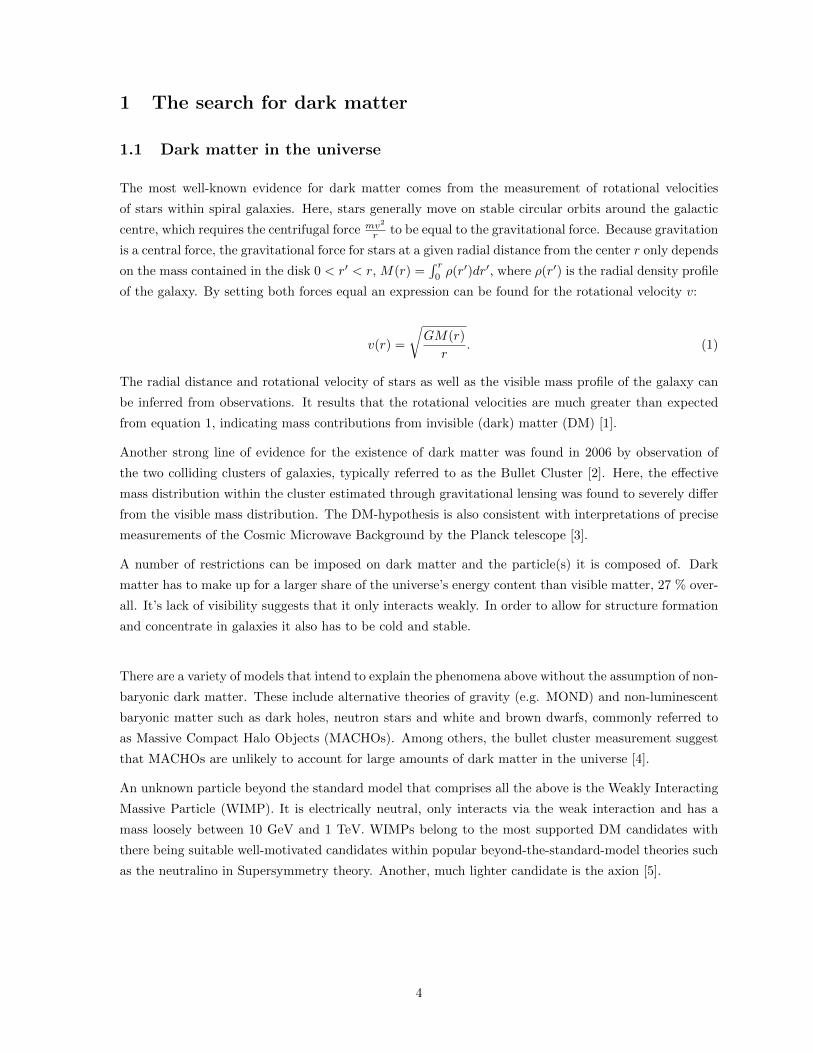
The most well-known evidence for dark matter comes from the measurement of rotational velocities
of stars within spiral galaxies. Here, stars generally move on stable circular orbits around the galactic
centre, which requires the centrifugal force mv2
r to be equal to the gravitational force. Because gravitation
is a central force, the gravitational force for stars at a given radial distance from the center r only depends
on the mass contained in the disk 0 < r′ < r, M(r) =∫ r
0ρ(r′)dr′, where ρ(r′) is the radial density profile
of the galaxy. By setting both forces equal an expression can be found for the rotational velocity v:
v(r) =
√GM(r)
r. (1)
The radial distance and rotational velocity of stars as well as the visible mass profile of the galaxy can
be inferred from observations. It results that the rotational velocities are much greater than expected
from equation 1, indicating mass contributions from invisible (dark) matter (DM) [1].
Another strong line of evidence for the existence of dark matter was found in 2006 by observation of
the two colliding clusters of galaxies, typically referred to as the Bullet Cluster [2]. Here, the effective
mass distribution within the cluster estimated through gravitational lensing was found to severely differ
from the visible mass distribution. The DM-hypothesis is also consistent with interpretations of precise
measurements of the Cosmic Microwave Background by the Planck telescope [3].
A number of restrictions can be imposed on dark matter and the particle(s) it is composed of. Dark
matter has to make up for a larger share of the universe’s energy content than visible matter, 27 % over-
all. It’s lack of visibility suggests that it only interacts weakly. In order to allow for structure formation
and concentrate in galaxies it also has to be cold and stable.
There are a variety of models that intend to explain the phenomena above without the assumption of non-
baryonic dark matter. These include alternative theories of gravity (e.g. MOND) and non-luminescent
baryonic matter such as dark holes, neutron stars and white and brown dwarfs, commonly referred to
as Massive Compact Halo Objects (MACHOs). Among others, the bullet cluster measurement suggest
that MACHOs are unlikely to account for large amounts of dark matter in the universe [4].
An unknown particle beyond the standard model that comprises all the above is the Weakly Interacting
Massive Particle (WIMP). It is electrically neutral, only interacts via the weak interaction and has a
mass loosely between 10 GeV and 1 TeV. WIMPs belong to the most supported DM candidates with
there being suitable well-motivated candidates within popular beyond-the-standard-model theories such
as the neutralino in Supersymmetry theory. Another, much lighter candidate is the axion [5].
4
1.2 Dark matter detection principles
There are a variety of avenues to detect DM and efforts have been made for over 20 years to detect
it. Some experiments have claimed WIMP detection, however, these findings are inconsistent with the
results of newer experiments with higher sensitivities. This indicates the tremendous challenge of dis-
tinguishing a weak dark matter signal from a variety of background sources in these experiments.
Collaborations like ATLAS are searching for dark matter by looking at collider events. In proton-proton
collisions a variety of particles are produced and detected. As WIMPs are expected to escape the detector
undetected, a produced WIMP would yield in a large missing momentum. So far, no WIMP-production
was indicated by these measurements [6].
Indirect detection experiments try to measure DM particle decay or annihilation by measuring their
decay products. IceCube e.g. is using a large ice target to detect multi-GeV neutrinos which could
originate from dark matter annihilating in the sun [7]. The Fermi Gamma Ray Space Telescope looks
for features in the cosmic gamma ray spectrum that could originate from DM-annihilation [8].
Strong limits on the WIMP-nucleon cross section are currently achieved by direct detection experiments.
Here, a target medium is set up on earth such that energy depositions of WIMPs in the target can be
detected. These manifest in scintillation, ionisation, heat production, or a combination of the prior.
Because of the low expected number of these events, detectors are operated for years and backgrounds
(i.e. events originating from any other source) have to be suppressed to an extremely high degree. This
involves both careful detector construction with highly radiopure materials as well as mechanisms to tag
events as background or signal on an event-by-event basis.
Examples include CRESST which measures phonons and scintillation light and uses the ratio as a pa-
rameter to discriminate between signal and background [9]. Another example is PICO which uses the
principle of a bubble chamber to detect WIMPs [10].
5

Figure 1: WIMP-Exclusion curves from current and planned argon and xenon experiments (taken from
[11]).
Liquid noble gases, specifically neon, argon, and xenon, are a suitable DM detection medium and differ-
ent direct detection experiments measure the scintillation and ionization yield that is caused by WIMPs
in these target materials. Many of these are operated in a dual-phase (liquid + gas) or TPC (Time
Projection Chamber) setup. Here, through application of an electric field, electrons freed by a WIMP-
nuclear-recoil are accelerated towards the gas, causing a secondary light signal to the primary scintillation
yield through gas discharge. The ratio between the primary and secondary signal carries information
about the type of particle that caused the event and is used for background rejection. Another advantage
is the strong achievable position reconstruction which can be used to tag events from e.g. radioactive
material in the detector walls. Both argon (e.g. DarkSide, ArDM, WArPs) and xenon (e.g. XENON,
LUX, PandaX) are commonly used as targets in TPCs. This technology currently achieves the strongest
limits among DM experiments with XENON1T (see figure 1).
Argon offers background rejection in a simple single-phase setup without external fields through pulse
shape discrimination (PSD). Here, freed electrons recombine and contribute to the scintillation yield,
which makes up the only signal channel. This setup is used by DEAP collaboration.
Because the exposure to dark matter scales linearly with the detector mass in the absence of backgrounds,
larger detectors are planned by many of the collaborations above to explore lower WIMP-nuclear cross
sections. DEAP started with a 7 kg liquid argon (LAr) prototype (DEAP-1) to demonstrate the potential
of PSD in a single-phase argon target [12] and currently operates a single-phase 3600 kg liquid argon
detector. A 20 tonne-LAr TPC is planned as the next generation liquid argon detector [13].
6

1.3 WIMP flux and exclusion curve
Direct detection dark matter experiments typically put limits on the WIMP-nuclear cross section as a
function of WIMP mass. Several assumptions enter such limit curves such as WIMPs accounting for the
full DM content of our universe. Assumption like this have to be made as the calculation of a cross sec-
tion requires knowledge of the WIMP-number density. A mass density of 0.3 GeV/cm3 is inferred from
cosmological considerations and hence a number density for a given WIMP mass can be calculated [14].
In principle, the WIMP mass also alters the WIMP-nuclear recoil spectrum, however due to the low
number of expected events given the current leading limits it is hard to make meaningful statements
about the shape of the spectrum.
The energy-deposition mechanism for WIMPs that direct detection experiments are sensitive to is elastic
scattering with a nucleus, i.e. a nuclear recoil. Assuming a nuclear form factor of 1, in the center-of-
momentum frame the WIMP scatters off a nucleus through an angle θ, with cos θ uniformly distributed
between -1 and 1. If the WIMP’s initial energy in the lab frame is Ei = Mχv2
2 , the nucleus recoils with
energy ER = Eir(1− cos θ) with r = 4MχMA
(Mχ+MA)2 , where MA is the mass of the target nucleus. ER for a
given Ei is therefore uniformly distributed between 0 and rEi and values from ER/r to ∞ contribute to
a ER < rEi. The recoil spectrum dRdER
can then be calculated with∫∞rEi
dR(Ei)Eir
, where 1/(Eir) normalises
the uniform distribution.
In order to obtain the distribution for Ei we assume that the WIMP’s velocities in the frame of the
galaxy follow the Maxwellian distribution. For direct detection experiments the velocities then have to
be corrected for earth’s velocity relative to the galaxy vE .
f(~v + ~vE) ∼ e(~v + ~vE)2/v20 (2)
where v0 = 220 ± 20 km/s is the local orbiting speed. The contribution from a velocity ~v to the event
rate per target nucleus is then
dR = σnχf(~v + ~vE)vd3~v. (3)
Here, nχ = is the WIMP number density. It is instructive (and reasonably accurate, as shown in [14])
to consider the simplified case of ignoring the earth’s velocity and the galaxy’s escape velocity (i.e.
integrating the velocity distribution from 0 to ∞). With E0 = Mχv202 the energy spectrum can now be
calculated
7
∫ ∞ER/r
dR
Eir=
∫ ∞ERr
1
(√πv0)3
σnχv1
Mχv2/2rev
2/v20 (4πv2dv) (4)
=2v0σnχ√πE2
0r
∫ ∞ER/r
e−Ei/E0dEi (5)
=2v0σnχ√πE0r
e−ER/E0r. (6)
Recoil energy (keV)0 20 40 60 80 100 120 140 160 180 200
)-1
tonn
e-1
yea
r-1
Eve
nt r
ate
(keV
4−10
3−10
2−10
1−10 50 GeV WIMP
100 GeV WIMP
500 GeV WIMP
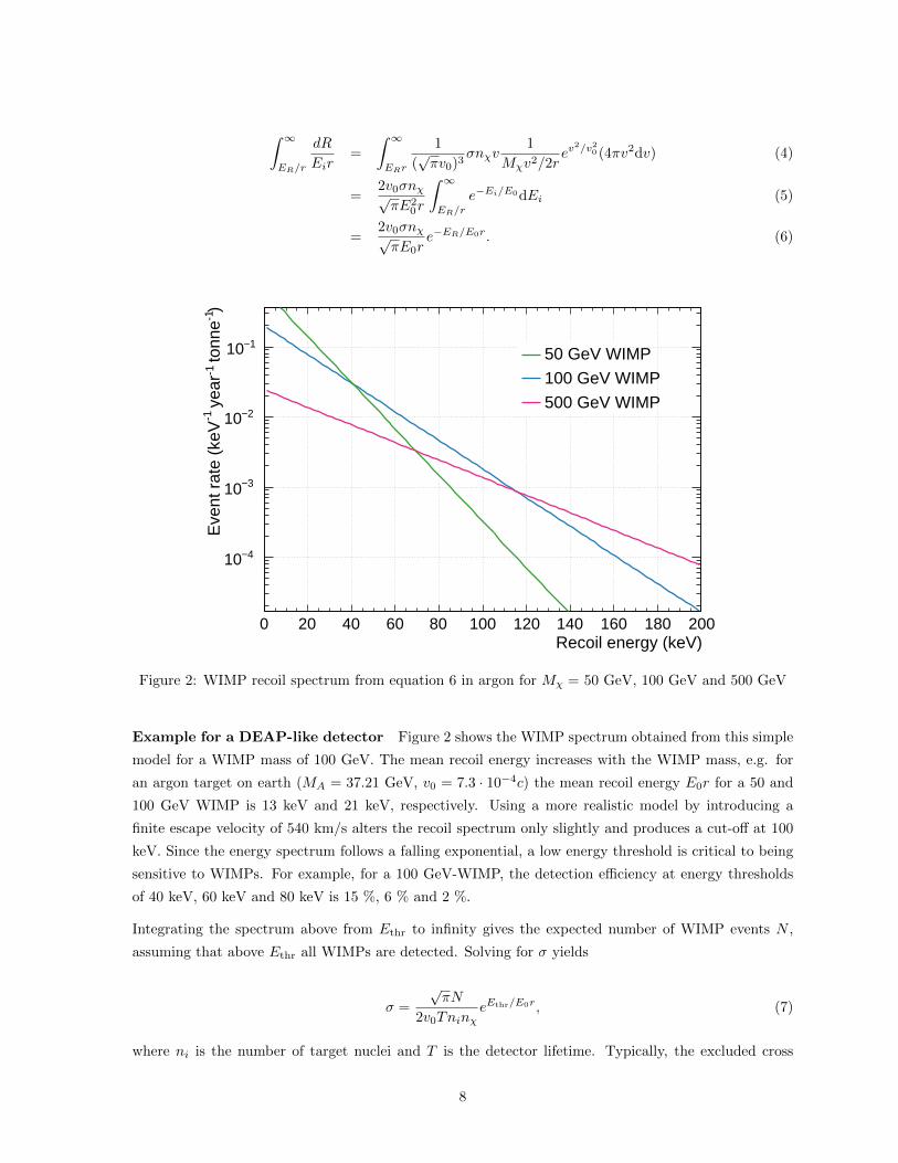
Figure 2: WIMP recoil spectrum from equation 6 in argon for Mχ = 50 GeV, 100 GeV and 500 GeV
Example for a DEAP-like detector Figure 2 shows the WIMP spectrum obtained from this simple
model for a WIMP mass of 100 GeV. The mean recoil energy increases with the WIMP mass, e.g. for
an argon target on earth (MA = 37.21 GeV, v0 = 7.3 · 10−4c) the mean recoil energy E0r for a 50 and
100 GeV WIMP is 13 keV and 21 keV, respectively. Using a more realistic model by introducing a
finite escape velocity of 540 km/s alters the recoil spectrum only slightly and produces a cut-off at 100
keV. Since the energy spectrum follows a falling exponential, a low energy threshold is critical to being
sensitive to WIMPs. For example, for a 100 GeV-WIMP, the detection efficiency at energy thresholds
of 40 keV, 60 keV and 80 keV is 15 %, 6 % and 2 %.
Integrating the spectrum above from Ethr to infinity gives the expected number of WIMP events N ,
assuming that above Ethr all WIMPs are detected. Solving for σ yields
σ =
√πN
2v0TninχeEthr/E0r, (7)
where ni is the number of target nuclei and T is the detector lifetime. Typically, the excluded cross
8
section at 90% confidence level is cited (such as in e.g. figure 1), i.e. the cross section at which the exper-
iment in 90% of cases would have measured more WIMP-like events than it actually did. In a detector
with zero expected backgrounds and zero measured WIMP-like events, this number of events N90 % C.L.
is with Poisson statistics P (N90 % C.L. > 0) = 0.9 → P (N90 % C.L. = 0) = 0.1 → exp(−N90 % C.L.) =
0.1→ N90 % C.L. = 2.3. Using formula 7, this can be converted into a limit on the cross section. With the
simplified model above using a 3 tonne argon target and an energy threshold of 60 keV this corresponds
to σ90 % C.L. = 1 · 10−46 for a runtime of 3 years.
Because this work is focused on the reduction of a background to the WIMP signal, it is instructive
to study the implications of a background on the excluded cross section. For example, if in the same
experiment 10 background events are predicted and 10 events are observed, the excluded cross section
at 90% confidence level would be σ90 % C.L. = 2.5 · 10−46 or more than double as high as in the prior
example. This is because the larger total number of total events (background + signal) n increases the
statistical uncertainties on the number of WIMP-events by√n. Therefore, in particular backgrounds
with a high rate have to be discriminated, i.e. excluded from the WIMP search in order to achieve a
competitive sensitivity, even if that means that a fraction of potential WIMP events will also be falsely
classified as background.
2 Argon as a dark matter detection medium
Natural argon consists to > 99.99 % of the stable isotopes 36Ar, 38Ar, 40Ar, with an 40Ar abundance of
99.6 % and is typically obtained by distillation of atmospheric gas. It also includes a (8.0± 0.6) · 10−16
fraction of beta-decaying 39Ar with a lifetime of 269 years (equivalent to a rate of (1.01± 0.08) Bq per
kg of natural argon) [15]. The 39Ar beta-spectrum has its endpoint at 565 keV [16].
melting point (at 1 bar) -189.35 C (83.80 K)
boiling point (at 1 bar) -185.9 C (87.30 K)
density at 0 C 1.784 g/l
density at -186 C 1.4 kg/l
Table 1: Properties of argon [17].
Gaseous, liquid and solid argon scintillates upon incident ionizing particles through the production of
excited dimers (Ar∗2-excimers) which ultimately decay under photon emission. Argon excitons Ar∗ are
produced either directly or indirectly by ionization and recombination:
9

Ar+ + Ar+→ Ar+2 (8)
Ar+2 + e− → Ar∗∗ + Ar (9)
Ar∗∗ → Ar∗ + heat (10)
This process is estimated to take about 500 ps. Light is then produced via
Ar∗ + Ar + Ar→ Ar∗2 + Ar (11)
Ar∗2 → 2Ar + hν. (12)
Here, hν is a UV photon and it is assumed that each excited argon dimer Ar∗2 emits a single photon.
Argon dimers can be produced in either a short-lived singlet or a long-lived triplet state. In the liq-
uid, the emission for both states is dominated by a peak at 128 nm with a width of approximately 10
nm [18]. Argon is transparent to the UV light which allows for good scalability of LAr detectors [19].
The argon scintillation properties vary under the type of interaction which excites the argon. Here, one
distinguishes between electronic and nuclear recoils. In an electronic recoil a particle scatters with an
electron in the shell of an argon atom. In a nuclear recoil a particle imparts some of its energy into
the argon nucleus. Nuclear recoils are the main interaction channel for neutrons and WIMPs, whereas
gammas and betas mainly interact via electronic recoils. Some of the different scintillation properties of
argon under both excitation types are believed to be due to the higher linear energy transfer (LET) of
nuclear recoils [18].
The average energy required to produce a single 128 nm or 9.7 eV-photon in an electronic recoil event
is 19.5 eV [20]. The light yield is found to be heavily reduced under high deposited energy densities or
LETs of the ionizing particle. A proposed non-luminescent deexcitation-mechanism under high exciton
densities is
Ar∗ + Ar∗ → Ar + Ar+ + e−, (13)
sometimes referred to as biexcitonic quenching [21]. The electron and ion can recombine and emit a
single photon instead of two for the two excitons. It was measured that for nuclear recoils the effective
scintillation light yield is 0.29 ± 0.03 times the light yield for electronic recoils for 6 keV electronic re-
coils [22]. The corresponding quenching factor for alpha particles is 0.74. In this work the energy unit
keVee, i.e. the estimated event energy under the assumption that the event is an electronic recoil is used.
The fraction of singlet excimer states was found to be higher at high LET [18]. Most notably, above
100 keVee about 75 % of excimers are produced in the singlet state for nuclear recoils vs 25 % for elec-
tronic recoils. The resulting difference in the time structure of the scintillation yield is big enough to
10

allow for particle type identification on a event-to-event basis (pulse shape discrimination). The precise
singlet-to-triplet ratios also depend on the particle energies and have been measured, among others, by
the SCENE collaboration for nuclear recoils [23] and the CLEAN collaboration for electronic recoils [24].
The lifetimes of the argon dimers themselves are independent of the type of excitation [18].
Literature values for the triplet lifetime range from 1300 to 1600 ns [12, 18, 24, 25]. The form of the
argon scintillation pulse shape also suggests the existence of an intermediate decay component with a
lifetime of around 40 ns and intensity of 10% which has been discussed for several years [26]. The effective
triplet lifetime strongly decreases as argon purity deteriorates. This can be explained by non-luminescent
deexcitation of Ar∗2 excimer states through collision with these impurities, e.g. for nitrogen:
Ar∗2 + N2 → 2Ar + N2 + heat. (14)
With a constant nitrogen contamination this deexcitation channel can be modelled with a simple rate law
that competes with the radiative deexcitation. This results in a light yield and triplet lifetime decrease
and was quantified for nitrogen in [27, 28] and oxygen contamination in [29]. Triplet excimers are more
exposed to this process than singlet excimers due to their smaller radiative decay rate. Therefore, high
purity of argon is of upmost importance for PSD, as it relies on the large difference in singlet and triplet
lifetimes.
3 The DEAP-3600 experiment
3.1 Detector overview
DEAP is using a single phase liquid argon target to directly detect WIMPs which makes it unique in
the otherwise TPC-dominated liquid scintillator dark matter search landscape. It was designed for a
target mass of 3600 kg and an energy threshold of 60 keV or 17 keVee for nuclear recoils. The projected
sensitivity to the WIMP-nucleon cross-section is 10−46 cm2 for 100 GeV WIMPs [30].
11

Figure 3: The DEAP-3600 detector design showing the acrylic vessel, light guides, and filler blocks, steel
shell, neck, and glove box (taken from [30]).
The detector is located 2 km underground in SNOLAB, Canada. Figure 3 shows an illustration of the
detector. The liquid argon is contained in a spherical vessel made of acrylic (plastic) with a radius of 85
cm. Advantages of acrylic include its high achievable radiopurity and its high concentration of hydrogen,
which acts as a neutron shield. It also tolerates a large thermal gradient which allows for photomultiplier
tube (PMT) operation at room temperature on the outer detector shell. The 255 Hamamatsu R5912
high quantum efficiency PMTs used for light detection are connected to the Argon by 45-cm long acrylic
light guides. A thin layer of 1,1,4,4-tetraphenyl-1,3-butadiene (TPB) is applied to the inner surface of
the acrylic vessel to shift the argon scintillation photons to the peak-efficiency-wavelength of the PMTs.
The target volume can be accessed through a vertical tube (neck). Cooling of the argon is achieved
through a liquid nitrogen filled cooling coil reaching down the neck. The detector is enclosed in a stain-
less steel vessel. The steel vessel is submerged in ultra-pure water which is used as a muon veto target
and viewed by 48 PMTs on the outer vessel side. Radioactive calibration sources can be placed close to
12

the detector through tubes inside of the water tank as shown in figure 13.
Because of an overfill and consecutive nitrogen leakage during the first fill attempt, the acrylic sphere
was not fully filled with argon during the consecutive argon fill. For all data discussed in this work, the
argon target mass is approximately 3300 kg.
3.2 Photomultiplier tubes
Photomultiplier tubes (PMTs) are sensitive light detectors that allow for single photon counting.
Figure 4: Illustration of the PMT work principle taken from [31].
A simplistic illustration of a PMT is shown on figure 4. A cathode, several dynodes and an anode are
arranged in a vacuum as shown. Incident photons strike the cathode and eject electrons due to the
photoelectric effect. These electrons are then consecutively accelerated towards a cascade of dynodes,
where upon each impact more electrons are emitted. The amplified electron charge is collected by the
anode and the resulting current is measured.
13
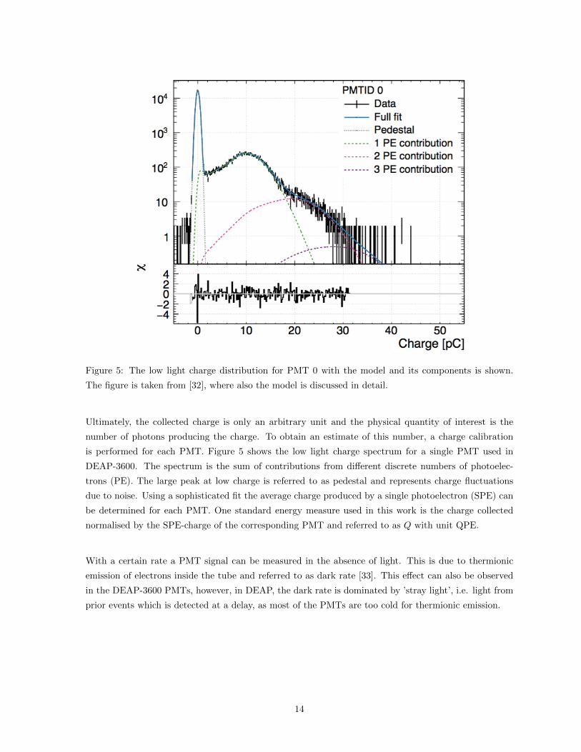
Figure 5: The low light charge distribution for PMT 0 with the model and its components is shown.
The figure is taken from [32], where also the model is discussed in detail.
Ultimately, the collected charge is only an arbitrary unit and the physical quantity of interest is the
number of photons producing the charge. To obtain an estimate of this number, a charge calibration
is performed for each PMT. Figure 5 shows the low light charge spectrum for a single PMT used in
DEAP-3600. The spectrum is the sum of contributions from different discrete numbers of photoelec-
trons (PE). The large peak at low charge is referred to as pedestal and represents charge fluctuations
due to noise. Using a sophisticated fit the average charge produced by a single photoelectron (SPE) can
be determined for each PMT. One standard energy measure used in this work is the charge collected
normalised by the SPE-charge of the corresponding PMT and referred to as Q with unit QPE.
With a certain rate a PMT signal can be measured in the absence of light. This is due to thermionic
emission of electrons inside the tube and referred to as dark rate [33]. This effect can also be observed
in the DEAP-3600 PMTs, however, in DEAP, the dark rate is dominated by ’stray light’, i.e. light from
prior events which is detected at a delay, as most of the PMTs are too cold for thermionic emission.
14

Figure 6: The measured probability for a typical PMT to observe a pulse following a primary pulse as a
function of both the second pulse’s charge (in units of the mean SPE charge) and of time. The primary
pulses were required to have a charge between 10 pC and 14 pC in this example taken from [32].
There is a low (typically 1 - 10%) probability for a PMT to produce a signal several hundreds of ns to a
few µs after an initial pulse. This is caused by residual gas in the tube and is referred to as afterpulsing:
accelerated electrons in a primary pulse can hit and ionise a residual gas molecule in the vacuum tube.
The ionised molecule is then accelerated towards a dynode, where upon impact it ejects electrons causing
a secondary pulse. The delay of the second pulse is positively correlated to the inertia of the ionised
molecule [34]. For DEAP-3600 an in-situ afterpulsing calibration is conducted: a light flash was induced
through a LED calibration system in the inner detector and the time and charge of pulses following the
initial pulse was measured. The probabilities for a secondary pulse as a function of their charge and
time delay are shown in figure 6. This measurement is used for both pulse shape validation, simulations
and an afterpulsing removal algorithm as described later.
3.3 DAQ & data flow
The data acquisition system (DAQ) records the signals of the 255 inner PMTs, the 4 PMTs in the neck
forming a veto-system and the 48 muon veto PMTs viewing the water tank. This work focuses on the
scintillation signal of the inner PMTs which is sampled at 250 MHz. Due to the high corresponding
data rate, data is not digitized and written continuously. A trigger module computes rolling integrals of
the PMT signals and adds them over all PMTs. Given this information the digitizers are triggered such
that a large share of 39Ar beta decays are not digitized while keeping all events in the WIMP region
of interest. The trigger information is always recorded. The data is stored in a DEAP-specific data
structure and saved in ROOT data format.
15

Time (ns)0 2000 4000 6000 8000 10000 12000
Cha
rge
(QP
E)
0
1
2
3
4
5
6
7
8
Figure 7: PMT trace for a typical electronic recoil event (QPE = 66.4). This is obtained by adding up
the pulses detected by the full PMT array.
The digitizers only digitze the part of the PMT waveforms where a signal threshold of about 10 % of the
SPE signal-height is crossed. These parts are referred to as pulses. The raw PMT signal, where a single
PE typically produces a pulse with a width of > 50 ns, is converted into delta-peaks with height of the
integrated charge of the pulse [32]. The time resolution achieved by the PMTs for standard SPE-pulses
is estimated to be < 2 ns. If multiple photons are seen by the same PMT within a short time window,
such that their raw PMT traces overlap, the time of the resulting subpeaks in the PMT traces are also
saved. For the rest of this work, these subpulses will be used exclusively and simply referred to as pulses.
An approximately linear dependency of the total detected charge Q in an event on the energy of the
detected particle is expected. This proportionality varies by particle type as the light yield in liquid
argon is particle dependent. The light yield for electronic recoils can be estimated through a fit of the
Q-spectrum with the theoretical 39Ar spectrum. The estimate for the light yield used in this work is
7.7±0.2 QPE per keV (or keVee) for electronic recoils. As an in-situ energy calibration for nuclear recoils
is not available, the light yield for nuclear recoils is obtained using the quenching factor measured by
the SCENE collaboration. This introduces a non-linearity into the energy calibration, as the quenching
factor is energy-dependent.
In addition to the number of photon estimated via charge, a more sophisticated measure, nnsc, is used
in this work. This estimate only considers pulses which are unlikely to be afterpulses and is obtained by
performing a Bayesian analysis on each pulse as described in detail in appendix B.
16
3.4 Background mitigation
There are a number of sources of events other than WIMPs in the DEAP-3600 experiment. Events
produced by some of these sources differ in their characteristics from WIMP-events and can be removed
with sophisticated data-cuts. Others could produce a signal indistinguishable from WIMPs and thus
have to be suppressed by the detector design.
Like WIMPs, neutrons interact via nuclear recoils and produce a similar argon scintillation time struc-
ture. Hence, neutrons present a particularly dangerous background to the experiment and low abundance
of neutron sources in all detector components has to be achieved. The hydrogenous inner detector ma-
terial additionally provides a strong shielding against neutrons coming from outside the detector [35].
Neutrons produced by cosmic muons are suppressed through placement of the detector underground and
the outer detector veto system.
Another background are alpha sources which can also produce an event time structure similar to WIMPs.
Even though highly radiopure materials are deployed, among others the unpure PMT glass-windows
cause an alpha and gamma-rate of multiple Bq. When exciting the liquid argon, both backgrounds
produce a signal far above the WIMP energy spectrum, however they still pose a relevant WIMP-
background as they can induce neutrons [36]. Also, alpha sources on the acrylic vessel surface or inside
the TPB layer could knock the daughter nucleus into the argon which then scatters in a low energy
nuclear recoil. Charged particles in the acrylic may produce Cherenkov light. These events will typically
cause a short flash in only few PMTs which is an incompatible topology to argon scintillation and can
be removed with corresponding data cuts.
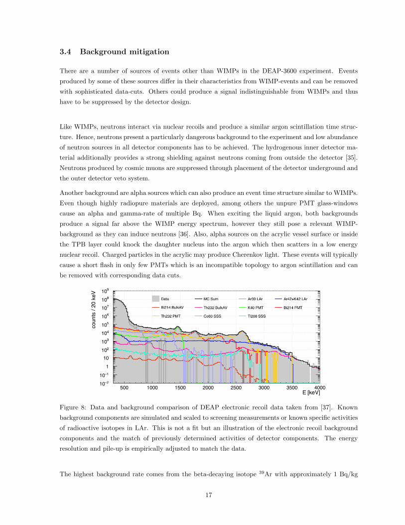
Figure 8: Data and background comparison of DEAP electronic recoil data taken from [37]. Known
background components are simulated and scaled to screening measurements or known specific activities
of radioactive isotopes in LAr. This is not a fit but an illustration of the electronic recoil background
components and the match of previously determined activities of detector components. The energy
resolution and pile-up is empirically adjusted to match the data.
The highest background rate comes from the beta-decaying isotope 39Ar with approximately 1 Bq/kg
17
of natural argon which dominates the overall event rate. This is illustrated by figure 8 which shows
electronic recoil background spectrum that is seen by DEAP. Here, below 500 keV, the 39Ar activity
surpasses all other backgrounds by over 3 orders of magnitude. Beta-radiation interacts in the argon
via electronic recoils and hence can be discriminated using PSD. 39Ar still limits the detector sensitivity
at low energies where PSD becomes less powerful. It also could produce a WIMP-like signal when
piled up with Cherenkov light. For this, algorithms are implemented that recognize features that are
characteristic for pile-up events.
The data selection cuts applied in this work are designed to select argon scintillation events and are
listed in appendix A.
4 The liquid argon scintillation pulse shapes in DEAP
PSD relies on understanding the difference in PMT traces produces by electronic and nuclear recoils.
While these differences are ultimately caused by the different singlet-to-triplet ratios caused by both
event types, the PMT traces in a real detector include components that are not due to the decay of
argon excimers. In order to understand how large the impact of these detector effects is and at which
time windows they occur, the average pulse shape is built by averaging over the PMT traces of a large
number of events. Pulse shapes are built over the full PMT array as well as for each for PMT individually
to isolate PMT-specific features. In addition to their importance for PSD, these can be used to validate
and estimate the afterpulsing rate (see appendix D), to extract an estimate of the dark rate from the pre-
trigger window of the pulse shapes, and to fit out the lifetime of the argon triplet lifetime in DEAP-3600
(see appendix C).
18

4.1 The 39Ar background pulse shape
4.1.1 Charge-based pulse shapes
/ ndf 2χ 1.429e+05 / 2372Prob 0tau [ns] 0.1± 1402 LatePE [PE] 1.301e+05± 2.828e+09 app3 0.00001± 0.06745
Time (ns)0 2000 4000 6000 8000 10000 12000
Tota
l cha
rge
(QPE
)
410
510
610
710 / ndf 2χ 1.429e+05 / 2372Prob 0tau [ns] 0.1± 1402 LatePE [PE] 1.301e+05± 2.828e+09 app3 0.00001± 0.06745
Average pulseshapeFit between 500 and 10000 nsTriplet componentAP Region 1AP Region 2AP Region 3AP of APAP of TPBTPB flourescenceDark noise
Figure 9: The average 39Ar pulse shape built using the pulse-charge over 600491 events. Also shown is
a fit function which highlights the different components of the pulse shape after 500 ns: argon triplet
scintillation, TPB fluorescence, afterpulsing and dark noise. Afterpulsing is subdivided into different
regions where each region represented by a Gaussian convoluted by the argon scintillation response in
time. The TPB fluorescence function is the exponential found in [38] convoluted by the argon singlet
and triplet component. The fit and its parameters are further discussed in appendix C.
Figure 9 shows the average pulse shape over the full PMT array for a dataset (run) taken five days after
the completion of the argon fill and the same pulse shape with a simple fit function highlighting the
different components. The fit function and its parameters are discussed in detail in appendix C, where
it is also used to extract and monitor the triplet lifetime over a one-year-dataset. The runs used have
a total duration of 5.6 h and 600491 events are used in the pulse shape. Data-cuts are applied such
that argon scintillation events between 30 keVee and 80 keVee are selected. Due to its dominant rate
practically all of these events are 39Ar electronic recoils. The pulse shape peaks sharply at the estimated
event time. This is expected because most of the argon singlet excimers decay within a few nanoseconds
after formation. The precise shape of this peak is determined by the PMT response functions and optical
properties of the detector. From 200 to 4000 ns the pulse shape decreases exponentially as triplet scin-
tillation dominates. At 5000 ns the number of pulses increases again because of afterpulsing and peaks
around 6500 ns. The tail of the pulse shape, at 13000 ns or almost 10 triplet lifetimes after the event
start is significantly above the dark noise level extracted from the pre-event level. Some of this might
be due to a delayed TPB fluorescence component that was investigated in [38,39]. The fit function here
19
uses the long-lived component of the TPB-fluorescence-model found by E. Segreto et al.
The delayed TPB light emission time structure is hard to extract from the electronic recoil data because
here, the delayed light intensity is dominated by the triplet component. However, by comparison of
pulse shape-fits that include and exclude the delayed TPB fluorescence component it can be concluded
that this component is likely also seen in DEAP with the χ2 of fits including the Segreto TPB model
being reduced by a factor of 3 (without adding any additional free fit parameters).
Another component that can be extracted from the pulse shapes is afterpulsing. While this is difficult in
the case of the first two afterpulsing regions as afterpulsing is very subdominant here, it is possible in the
case of AP region 3. Here, the mean, width and height of the Gaussian that used to describe the AP are
left as free parameters in the fit above. The fit result can then be compared to the time structure that
is expected from the afterpulsing calibration. Here, it is found that the mean of the Gaussian is shifted
against what is expected from the calibration by 500 ns. The origin of this shift has not been resolved yet.
Time (ns)0 2000 4000 6000 8000 10000 12000
Tot
al c
harg
e (Q
PE
)
410
510
610
710 Electronic recoil data
Electronic recoil simulation
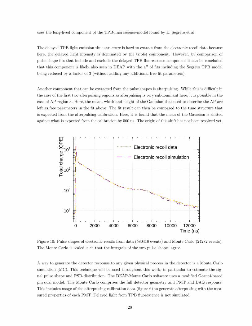
Figure 10: Pulse shapes of electronic recoils from data (580416 events) and Monte Carlo (24282 events).
The Monte Carlo is scaled such that the integrals of the two pulse shapes agree.
A way to generate the detector response to any given physical process in the detector is a Monte Carlo
simulation (MC). This technique will be used throughout this work, in particular to estimate the sig-
nal pulse shape and PSD-distribution. The DEAP-Monte Carlo software uses a modified Geant4-based
physical model. The Monte Carlo comprises the full detector geometry and PMT and DAQ response.
This includes usage of the afterpulsing calibration data (figure 6) to generate afterpulsing with the mea-
sured properties of each PMT. Delayed light from TPB fluorescence is not simulated.
20

The 39Ar electronic recoil background is a suitable event source to verify the MC given its high abundance
of events. Figure 10 shows the pulse shapes obtained from data and Monte Carlo. Here, the same cuts
are applied to both datasets. Up to 6000 ns there is very good agreement between the two pulse shapes.
Above 6000 ns, the data-pulse shape is approximately 10 % higher than the MC-pulse shape. A plausible
explanation for this could be the missing TPB fluorescence simulation, which only becomes significant
late in the pulse shape (see figure 9).
4.1.2 Afterpulsing-corrected pulse shapes
In addition to charge, the photon count nnsc will be used as an estimate for the number of photons in
the PMT traces. Because afterpulsing and scintillation follow very different distributions in time, the
nnsc-pulse shape is expected to differ from the charge-weighted pulse shape.
/ ndf 2χ 1.413e+04 / 748Prob 0tau [ns] 0.1± 1382 LatePE [PE] 1.937e+05± 5.918e+09
Time (ns)0 2000 4000 6000 8000 10000 12000
scT
otal
n
410
510
610
710
810 / ndf 2χ 1.413e+04 / 748
Prob 0tau [ns] 0.1± 1382 LatePE [PE] 1.937e+05± 5.918e+09
Average pulseshapeFit between 500 and 3500 nsTriplet componentTPB flourescenceDark noise
Figure 11: Pulse shape of electronic recoil events using the photon count nnsc.
Figure 11 shows the pulse shape from the same run using nnsc instead of charge with the same fit func-
tion without the afterpulsing components. The pulse shape behaves similar to the charge-weighted pulse
shapes until 5000 ns. From 5000 to 6000 ns the pulse shape declines sharply and stays then relatively
flat until end of the pulse shape. Beyond 5000 ns the behaviour therefore differs severely from the
scintillation model. The estimated loss of the scintillation yield, i.e. difference between the integral of
the fit function and the data from 0 to 13000 ns is 3%. A possible explanation for this feature could be
the estimator that is used to calculate nnsc: nnsc is set to the value that maximizes its posterior (also
known as a maximum a posteriori (MAP) estimator). At 6000 ns afterpulsing is on average more likely
than scintillation as indicated by the afterpulsing peak in the charge-weighted pulse shapes. Because
21

nnsc is set to its most likely value, the scintillation contribution will be ignored in many cases where it
still makes up a significant (but subdominant) share of the total pulse shape. An alternative explanation
would be that the simplifications made by the model cause this bias.
/ ndf 2χ 2.793e+04 / 748Prob 0tau [ns] 0.1± 1345 LatePE [PE] 3.188e+05± 1.583e+10
Time (ns)0 2000 4000 6000 8000 10000 12000
scT
otal
n
410
510
610
710
810 / ndf 2χ 2.793e+04 / 748Prob 0tau [ns] 0.1± 1345 LatePE [PE] 3.188e+05± 1.583e+10
Average pulseshape
Fit between 500 and 3500 ns
Triplet component
TPB flourescence
Dark noise
Figure 12: Pulse shape of electronic recoil events using the photon count nnsc estimated using an MMSE
estimator.
To test the first hypothesis, an nnsc-variation is implemented that uses the same physical model, but
estimates nnsc as its mean over the posterior (minimum-mean-squared-error or MMSE estimator). The
MMSE-pulse shape (figure 12) is much more compatible with a scintillation pulse shape and does not
show a sharp drop as in figure 11. This suggests that this feature is indeed a threshold effect produced
by the estimator and indicates that the model describes the data appropriately. It should be noted
that the MMSE-pulse shape does not match the fit function perfectly either. In particular, the TPB
fluorescence component appears to be lower in data than in the parameters found in Segreto’s paper [38].
It is unclear whether that is due to a bias in the estimator or whether the TPB fluorescence trace indeed
differs from the values found by Segreto.
The nnsc photon count using the MMSE estimator will later be used as a photon estimate for PSD
and requires a separate energy calibration. This has not been done yet by fits of for example the 39Ar-
spectrum. The relative LYs between charge and nnsc can still be found by finding the average charge that
correspond to a nnsc-value. The LY in the energy region of interest found this way is 7.0NSC±0.3nsc/keV
for the MMSE estimate, where NSC is the unit of nnsc.
For a more detailed comparison of the MAP and MMSE estimators in the context of the PE counting
22

problem, see appendix B.4.
4.2 The nuclear recoil signal pulse shape
For PSD, the difference between the nuclear and electronic recoil pulse shape is critical. The nuclear
recoil pulse shape can not be built easily from data as nuclear recoils in the liquid argon are suppressed
by detector design. Nuclear recoil datasets can still be produced in two ways: placement of a neutron
source close to the detector and Monte Carlo simulations. Additionally, pulse shapes can be built using
a model of the scintillation and PMT-response time structure.
4.2.1 Charge-based pulse shapes
To see what a WIMP interaction in the detector could look like, a neutron source calibration is performed.
Neutrons, like WIMPs, interact via nuclear recoils.
Neutrons can be produced by a composite source consisting of an alpha emitter and a light element.
Typically, the alpha-emitter and light element used are Americium (241Am) and Beryllium (9Be), re-
spectively, forming an AmBe source [40]:
241Am→ 237Np + 4He (15)
9Be + 4He→ 12C + n. (16)
Here the C-atom can be produced in an excited state which quickly decays emitting a 4.4 MeV gamma-
ray. The AmBe-neutron spectrum has a non-trivial multimodal form that extends down to low energies.
23
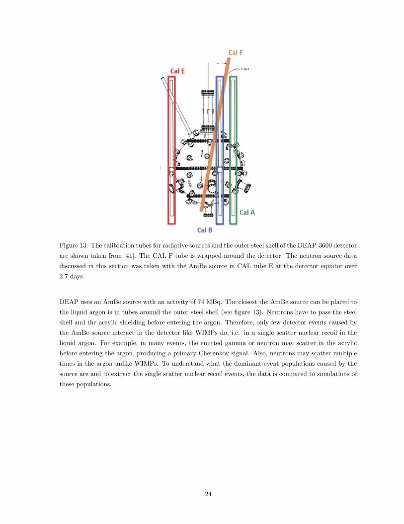
Figure 13: The calibration tubes for radiative sources and the outer steel shell of the DEAP-3600 detector
are shown taken from [41]. The CAL F tube is wrapped around the detector. The neutron source data
discussed in this section was taken with the AmBe source in CAL tube E at the detector equator over
2.7 days.
DEAP uses an AmBe source with an activity of 74 MBq. The closest the AmBe source can be placed to
the liquid argon is in tubes around the outer steel shell (see figure 13). Neutrons have to pass the steel
shell and the acrylic shielding before entering the argon. Therefore, only few detector events caused by
the AmBe source interact in the detector like WIMPs do, i.e. in a single scatter nuclear recoil in the
liquid argon. For example, in many events, the emitted gamma or neutron may scatter in the acrylic
before entering the argon, producing a primary Cherenkov signal. Also, neutrons may scatter multiple
times in the argon unlike WIMPs. To understand what the dominant event populations caused by the
source are and to extract the single scatter nuclear recoil events, the data is compared to simulations of
these populations.
24

Time (ns)0 2000 4000 6000 8000 10000 12000
Tot
al c
harg
e (Q
PE
)
10
210
310
410
510 AmBe source data
Nuclear recoil simulation
Electronic recoil data
Figure 14: Pulse shapes of the AmBe calibration data, a nuclear recoil simulation and electronic recoil
data using the are shown. Events with energies between 15 keVee and 60 keVee and Fprompt > 0.6 for
AmBe data are selected. The simulated (4684 events) and electronic recoil pulse shape (600491 events)
are scaled down to match the integral of the AmBe-pulse shape (1622 events).
Another way to produce a nuclear recoil pulse shape is via a Monte Carlo simulation (Monte Carlo or
MC) of 40Ar nuclei (m = 37 GeV) in the liquid argon. Like WIMPs, the nuclei scatter in the argon in
nuclear recoils. The singlet-to-triplet ratios of argon dimers produced by the nuclear recoils are set to
the values measured by the SCENE collaboration [23]. Figure 14 shows the pulse shape of simulated
recoils uniformly distributed throughout the argon with a flat momentum distribution from 20 to 200
keV. This is compared to the AmBe-calibration data and an electronic recoil pulse shape. Because the
AmBe calibration data is still dominated by 39Ar events, the nuclear recoil events are selected using a
cut on the prompt fraction of charge, Fprompt. This parameter is also used for pulse shape discrimination
and is discussed in detail in section 5.1.
As expected, the singlet peak is higher for the nuclear recoil signal. The triplet component in the nu-
clear recoil event traces is suppressed compared to electronic recoils such that two afterpulsing region
at approximately 500 ns and 2000 ns can be seen. As the afterpulsing in electronic recoil events is
dominated by afterpulsing of the narrow and early singlet peak, the afterpulsing peak in the nuclear
recoil pulse shape at 6000 ns is narrower and centered around an earlier time relative to the afterpulsing
in the electronic recoil pulse shape. The AmBe and Monte Carlo pulse shape do not match at several
times in the pulse shapes. Firstly, the AmBe singlet peak is broader than the singlet peak of electronic
recoil data and simulated nuclear recoils. This might be due to events where neutrons scatter multiple
times in the detector. As noted above, the position of the afterpulsing region around 6500 ns is shifted
25

approximately 500 ns. This can also be observed in figure 14 and is expected because the simulation
relies on the calibration to generate afterpulses. Also, the tail of the pulse shape is lower in simulation
than for the AmBe data. This might be explainable by the missing TPB fluorescence simulation in
Monte Carlo.
4.2.2 Afterpulsing-corrected pulse shapes
Time [ns]0 2000 4000 6000 8000 10000 12000
scT
otal
n
210
310
410
510
610
MAP-estimator
MMSE-estimator
Figure 15: nnsc - pulse shapes of simulated nuclear recoils.
For electronic recoil data a time-dependent bias was found under the MAP-PE counting scheme. This
bias is also present in the nuclear recoil simulation as shown figure 15. Here, the pulse shape under the
MAP and MMSE estimator are compared. The threshold effect disappears as nnsc is estimated over the
mean of the posterior, which confirms that the bias is caused by the default estimator.
4.3 Mathematical pulse shape model
As shown with the fit in figure 9, the pulse shape can be modelled by a mathematical model. In this
section, this function is extended to describe the full pulse shape including the prompt peak of nu-
clear and electronic recoil events. This model will be used later to build timing PDFs and evaluate a
likelihood-based PSD parameter.
The only difference in the electronic and nuclear recoil PDFs should be the underlying singlet-to-triplet
ratio. Therefore, it is convenient to build PDFs for the singlet and triplet component separately and
to mix them with distinct ratios to obtain the electronic and nuclear recoil PDF. Here, it is assumed
26
that the shape of these PDF does not depend on e.g. the event energy or position, such that the PDFs
can be used to describe all argon scintillation events. Because afterpulsing and TPB fluorescence scale
with the amount of argon scintillation light, the time responses of these components can be included
by convoluting their response with singlet and triplet exponentials. The models used here are the same
that are used for the pulse shape fit described in appendix C. The remaining component that does not
scale with the energy of an event is dark noise and should therefore be added separately.
Time (ns)0 2000 4000 6000 8000 10000 12000 14000 16000
)-1
Pro
babi
lity
dens
ity (
ns
7−10
6−10
5−10
4−10
3−10
2−10
Time (ns)0 2000 4000 6000 8000 10000 12000 14000 16000
)-1
Pro
babi
lity
dens
ity (
ns
6−10
5−10
4−10
3−10
2−10
Time (ns)0 2000 4000 6000 8000 10000 12000 14000 16000
)-1
Pro
babi
lity
dens
ity (
ns
6−10
5−10
4−10
3−10
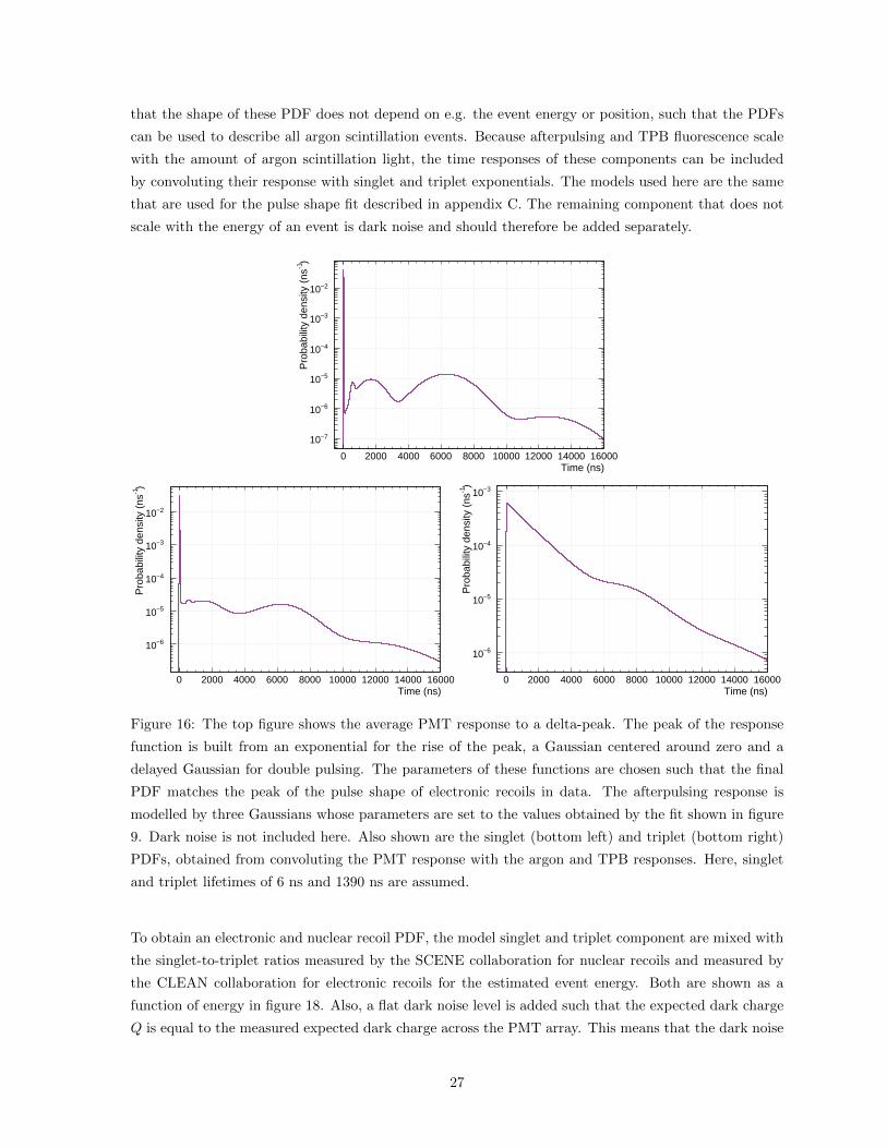
Figure 16: The top figure shows the average PMT response to a delta-peak. The peak of the response
function is built from an exponential for the rise of the peak, a Gaussian centered around zero and a
delayed Gaussian for double pulsing. The parameters of these functions are chosen such that the final
PDF matches the peak of the pulse shape of electronic recoils in data. The afterpulsing response is
modelled by three Gaussians whose parameters are set to the values obtained by the fit shown in figure
9. Dark noise is not included here. Also shown are the singlet (bottom left) and triplet (bottom right)
PDFs, obtained from convoluting the PMT response with the argon and TPB responses. Here, singlet
and triplet lifetimes of 6 ns and 1390 ns are assumed.
To obtain an electronic and nuclear recoil PDF, the model singlet and triplet component are mixed with
the singlet-to-triplet ratios measured by the SCENE collaboration for nuclear recoils and measured by
the CLEAN collaboration for electronic recoils for the estimated event energy. Both are shown as a
function of energy in figure 18. Also, a flat dark noise level is added such that the expected dark charge
Q is equal to the measured expected dark charge across the PMT array. This means that the dark noise
27

fraction is smaller for high energy events than for low energy events.
Time (ns)0 2000 4000 6000 8000
)-1
Pro
babi
lity
dens
ity (
ns
6−10
5−10
4−10
3−10
2−10 Model (singlet + triplet + noise)
Electronic recoil data
Time (ns)0 2000 4000 6000 8000 10000 12000 14000 16000
)-1
Pro
babi
lity
dens
ity (
ns
5−10
4−10
3−10
2−10Model (singlet + triplet + noise)
AmBe calibration data
Figure 17: The combined model scintillation PDFs for 15.36 keVee electronic recoils (left) and nuclear
recoils (right) are shown. The PDFs are compared to pulse shapes built from electronic recoils and
AmBe data between 100 QPE (13.4 keVee) and 120 QPE (16.0 keVee).
An example for a pair of model-PDFs is shown in figure 17. This is obtained by mixing the singlet and
triplet model PDFs (figure 16) with the measured singlet fractions at 15.36 keVee (0.29 for electronic
recoils, 0.69 for nuclear recoils). The dark noise level is estimated from the early window of the pulse
shape. To verify the model, this is compared to pulse shapes from data. The electronic recoil PDF
agrees very well with the pulse shape. This implies that both the models used for the singlet and triplet
time structure as well as the singlet-to-triplet ratio measured by the CLEAN collaboration describe the
data well. For nuclear recoils, the triplet component in data appears to suppressed when compared to
the model. This can be explained by the Fprompt-cut that are used, which biases the event selection
towards events with low late-light-intensity. The low statistics of the nuclear recoil data in the narrow
energy range used here prohibits to test the agreement at later times.
5 Pulse shape discrimination
As discussed in section 1.3, even a well understood background with a background model significantly
affects the sensitivity of a direct detection experiment. Therefore, in order to set a competitive limit
on the WIMP-nuclear recoil cross section, DEAP-3600 has to discriminate its background of more than
108 39Ar events per year and keVee (see figure 8) in its energy region of interest from nuclear recoils.
This is possible by excluding events from the WIMP-search that are likely to emerge from the electronic
recoil PDF. For this, parameters have to be found that capture the similarity of an event trace to the
PDFs shown in the prior section. In addition to background suppression, PSD also allows for isolation
of different detector backgrounds for calibration purposes and detector studies.
28

)ee
Reconstructed energy (keV0 10 20 30 40 50 60
Sin
glet
frac
tion
0.0
0.1
0.2
0.3
0.4
0.5
0.6
0.7
0.8
0.9
1.0
Electronic recoilsNuclear recoils
Figure 18: Singlet fractions for electronic and nuclear recoils measured by the CLEAN [23] and SCENE
[24] collaboration, respectively. The nuclear recoil energies are converted to keVee using the quenching
factor measured by SCENE.
PSD is ultimately enabled by the different singlet-to-triplet ratios for electronic and nuclear recoils which
are found to be energy dependent. The singlet fraction for both interaction types are shown in figure
18. Below 5 keVee, the singlet and triplet fractions of both interactions are approximately equal and
diverge slowly at higher energies. Therefore, PSD is only viable above an energy threshold and only
becomes more powerful at higher energies. With an anticipated energy threshold of 18 keVee, in DEAP,
the limiting factor for PSD at low energies is the low statistics of photons in the events. This is because
for an electronic recoil at low energies it is more likely that a large fraction of triplet excimers decay at a
time scale that is typical for singlet excimers and the event mimics a nuclear recoil this way. PSD there-
fore becomes significantly more powerful at higher energies, despite the singlet-to-triplet ratio staying
constant here.
The energy threshold in DEAP-3600 for the WIMP-search is directly set by the energy at which the 108
39Ar per keVee and year can be reduced to our design goal of 0.2 events in the WIMP search region. This
lower bound of the WIMP search box is of particular importance to the sensitivity of the experiment
because of the exponential decrease of the WIMP nuclear recoil spectrum. Using a PSD parameter
that achieves strongest separation of electronic and nuclear recoils can therefore notably increase this
sensitivity. In the following section different PSD parameters are introduced and evaluated with regard
to their viability for the DEAP-3600 dark matter search analysis.
29
5.1 Prompt-window-based discrimination
A simple discrimination parameter Fprompt is defined as the fraction of charge in the prompt time window
[tstart, tprompt] of an event. Because the prompt peak is dominated by singlet photons, this discriminator
can be interpreted as a simple estimate for the singlet fraction in an event and is therefore on average
higher for nuclear recoils than for electronic recoils.
Fprompt =∑i
ni[tstart < ti < tprompt]/ntotal (17)
Here, ni refers to the estimated number of photons in the subpulse at time ti. This discriminator
introduces two free parameters: the start of the integration windows tstart, the end of the prompt inte-
gral tprompt and the end of the total integration window tlate. These parameters have been found to be
optimal at tstart = −28 ns and tprompt = 60 ns [42]. For ntotal it is summed over photons in [-28 ns, 10 us].
Prompt-window-based discriminators are well established for PSD in liquid argon scintillation and are
used by dark matter experiments, most notably DEAP and DarkSide in their most recent publications
[11, 43]. Advantages of prompt-window-based discrimination include that they are computationally
inexpensive. Also, due to their simplicity, analytical and physically-motivated models can be developed
to describe their distributions [44]. For the rest of this work Fprompt refers to the parameter using charge,
whereas F scprompt refers to the prompt-window-based discriminator using nnsc.
5.2 Likelihood-based discrimination
A disadvantage of Fprompt is that it bins the highly resolved timing information of an event into prompt
and late light. A PSD-parameter that makes use of the full information contained in the event pulse shape
should in theory achieve superior discrimination and therefore improve the sensitivity of the experiment.
This can be implemented by weighting pulses in a particle identification parameter S with a function
w(ti) that depends on the position of pulses in time, as described in [45] by E. Gatti and F. de Martini:
SGatti =∑i
w(ti)ni. (18)
Here, it was shown that the relative variance of the separation between SGatti produced by electronic
and nuclear recoils is minimized, if
wSGatti(ti) =p(t)nr − p(t)er
p(t)nr + p(t)er, (19)
p(t)er and p(t)nr are the PDFs of electronic and nuclear recoils in time at the estimated event energy.
Intuitively, its modulus is a measure for how much information a photon at time t contains with regard
to the event being an electronic or nuclear recoil. For example, if both PDFs are equal at some time,
the weight function w(t) becomes zero and photons arriving at this time would not affect SGatti. The
30

sign of w(t) indicates whether photons arriving at t are more indicative of the event being an electronic
(negative sign) or nuclear recoil (positive sign). For the rest of this work, w(t) will be referred to as the
photon weight, or simply weight.
Another PSD-parameter that takes into account the precise PMT event-trace is the likelihood ratio
between an event being an electronic and nuclear recoil. According to the Neyman-Pearson lemma,
the likelihood ratio Λ, i.e. the ratios of likelihoods of an observation under two different hypothesis
θ0, θ1, is the most powerful test of θ0 against θ1 at a given significance level [46]. Indeed, it was shown
in [47] that in a simulation of electronic and nuclear recoils in the CLEAN-detector, a likelihood-based
PSD-discriminator can perform better than a prompt-window-based discriminator. Here, the likelihood
ratio between the electronic and nuclear recoil-hypothesis was defined by
Λ({t1..tn}) =L(θnr| {t1..tn})L(θer| {t1..tn})
, (20)
where θnr and θer denote the hypothesis that the event is produced by a nuclear or electronic recoil,
respectively and {t1..tn} are the photon arrival times. If the photons are drawn independently from the
PDFs, as they are for dark noise and argon scintillation, the total event likelihood can be written as the
product of the photon arrival likelihoods:
L(θ| {t1..tn}) = L(t1|θ)..L(tn|θ). (21)
For computational reasons it is advantageous to use the log-likelihood ratio. With L(θnr|ti) = p(t)nr
and L(θer|ti) = p(t)er above, log Λ can be rewritten as a function of the log ratio of the two PDFs
wLrecoil(ti) = log p(t)nr
p(t)er. Also, whereas for integer estimates for the number of photons, like nsc, Λ can
be evaluated directly, its definition can also be extended for continuous estimates like Q by weighting
each pulse with its photon-estimate. Note that under this extension, L is not strictly a likelihood, as
the likelihood to see a non-integer number of photons is zero. With this, we get
log Λ ({t1..tn} , {n1..nn}) =∑i
niwLrecoil(ti). (22)
From equation 22 it can be seen that wLrecoil(t) takes the place of a weighting function, as in the definition
of the Gatti parameter. It can be seen that both wSGatti(t) and wLrecoil(t) can be written in terms of the
ratio of both PDFs x = p(t)nr
p(t)er. Expanding around x = 1, where both PDFs are equal yields
∑i
wLrecoil(ti) = log x = (x− 1)− 1
2(x− 1)2 +
1
4(x− 1)3 +O(x− 1)4 (23)
and
∑i
wSGatti(ti) =x− 1
x+ 1∝ (x− 1)− 1
2(x− 1)2 +
1
3(x− 1)3 +O(x− 1)4. (24)
31
Therefore, the weights of photons under Lrecoil and SGatti coincide up to order O(x− 1)3. Indeed, it is
shown in appendix E that the weighting functions of Lrecoil and SGatti coincide very closely. Therefore
only Lrecoil is discussed in the main part of this work.
It has several advantages to not use Λ directly as a PSD parameter, but to use the following rescaling:
Lrecoil =1
2
(1 +
log Λ ({t1..tn} , {n1..nn})ntotal
)(25)
=1
2
(1 +
∑i niw(ti)
Lrecoil
ntotal
). (26)
Here, normalising by the total number of photons ensures that scaling an event ni → ani does only affect
Lrecoil through a potential dependence of the PDFs on the event energy. Because the singlet-to-triplet
ratios produced by electronic recoils stay flat above 20 keVee, so should their PDFs which should cause
Lrecoil to be distributed within constant bands for both interaction types. Another advantage of the
definition in equation 26 is that here, Fprompt can be expressed in terms of Lrecoil if weighting function
wFprompt(t) is assumed
wFprompt(t) =
1, if tstart < ti < tprompt
−1, if tprompt < ti < tlate
0, otherwise,
(27)
because then
Lrecoil =1
2(1 +
∑i niw
Fprompt(t)
ntotal) (28)
=1
2
ntotal +∑i niw
Fprompt(ti)
ntotal(29)
=1
2
∑i ni[tstart < ti < tlate] +
∑i ni[tstart < ti < tprompt]−
∑i ni[tprompt < ti < tlate]
ntotal(30)
=1
2
2∑i ni[tstart < ti < tprompt]
ntotal(31)
= Fprompt. (32)
Therefore, the weights that are assigned to photons under a prompt-window-based parameters can be
directly compared to the weights used by Lrecoil.
While Lrecoil for a general w(t) can take values between +∞ and −∞ it is later found that practically all
liquid argon scintillation events under wLrecoil(t) take values in [−ntotal, ntotal]. Therefore, an additional
advantage of the rescaling above is that it projects Lrecoil from [−ntotal, ntotal] into [0,1]. This allows to
fit the Lrecoil-distributions with a gamma-function, which is only defined for positive values, as it will
32
be done later in this work. For the rest of this work Lrecoil is referring to the parameter using charge,
whereas Lscrecoil refers to the likelihood-based discriminator using nnsc.
5.3 Evaluation of the photon weight
The construction of a continuous w(t) requires a pair of electronic and nuclear recoil PDFs. These PDFs
can be built from a complete detector Monte Carlo, from data and from an effective model. Because
PDFs will show some method-dependent features, w(t) should only be formed by PDFs that were built
by the same method. As it will be discussed in section 5.4.2, extraction of a clean set of WIMP-like
events from the AmBe calibration data has not been achieved to-date. Therefore only log-ratios built
from Monte Carlo and a simple model are shown in the section below and used in Lrecoil.
Also, as it was shown above, the different photon estimators (Q, nnsc) differ in their pulse shapes.
Therefore, separate PDFs have to be built depending on the photon estimator used.
5.3.1 The photon weight under Model PDFs
Because of energy dependency of the singlet and triplet fractions of electronic recoils, the PDFs used
should depend on the estimated event energy. Therefore, both PDFs are built by mixing the singlet and
triplet component with weights that are looked up from a table of the SCENE measurement for nuclear
recoils and CLEAN measurement for electronic recoils as it was shown in section 4.3.
33

Time (ns)0 2000 4000 6000 8000 10000 12000 14000 16000
Pho
ton
wei
ght w
(t)
1.0−
0.5−
0.0
0.5
1.0(t) (Argon)recoilL
w(t) (Argon + DN)recoilL
w(t) (Argon + DN + TPB)recoilL
w(t) (Argon + DN + TPB + AP)recoilL
w(t)promptF
w
Figure 19: Photon weight-functions for models taking into account different components of the detector
response at 15.36 keVee are shown. This includes argon scintillation (Argon), dark noise (DN), TPB
fluorescence (TPB) and afterpulsing (AP). This is compared to the log-likelihood that is assumed by
Fprompt. The weight function can be interpreted as follows: pulses time where w(t) > 0 or w(t) < 0
are more likely to be detected for nuclear recoil or electronic recoil events, respectively. Pulses that are
detected at a time where w(t) = 0 are equally likely to be seen in nuclear and electronic recoils.
The log-ratio computed using the resulting PDFs is shown in figure 19. Here, different models for the
detector response are assumed, such that the impact of the different components can be seen. In ev-
ery case, the log-ratio is sharply peaked at t = 0, where most of the singlet light is detected. For a
timing model only consisting of exponentials for the singlet and triplet component, the likelihood func-
tion drops sharply after the singlet peak and stays constant afterwards. This can be explained by the
large differences in the respective lifetimes: at later times, the singlet component becomes negligible
and the log-ratio can be approximated by the log-ratio of triplet fractions for electronic and nuclear
recoils. It should be noted that this shape is similar to the step-function that is used as weight for
Fprompt. Therefore, in an detector with a delta-like response function and no noise, a prompt-window-
based discriminator and a likelihood-based discriminator should almost identical results, given that they
use pulses in the time windows.
For a model that additionally takes TPB fluorescence and dark noise into account, the log-likelihood
ratio converges towards zero at later times. This is the expected behaviour, as the signal-to-noise ratio
becomes worse here. Also, by including TPB fluorescence, late light loses some of its information content.
Including afterpulsing in the model adds bumps to the likelihood-ratio at the times of high afterpulsing
probability (compare with PMT response in figure 16). This makes sense, because both singlet and
triplet light cause afterpulsing. This effect is so large that for a brief time around 6500 ns pulses do
not carry any information with regard to the nature of the event. Afterwards, the photon weight drops
34

again as the afterpulsing of the triplet component is delayed relative to the afterpulsing of the singlet
component, such that the signal-to-noise ratio becomes better than without afterpulsing.
Time (ns)0 2000 4000 6000 8000 10000 12000 14000 16000
Pho
ton
wei
ght w
(t)
0.8−
0.6−
0.4−
0.2−
0.0−
0.2
0.4
0.6
0.8
-based disc.sc
(t) used for nrecoilLw
(t) used for Q-based disc.recoilLw
Figure 20: Photon weight-functions that are used for the PSD parameters evaluated in the following
section at 15.36 keVee are shown. For charge (Q)-based discrimination the model PDFs include argon
scintillation, dark noise and afterpulsing. For the nnsc photon estimators, only argon scintillation and
dark noise are considered.
The wLrecoil(t) that will be used for PSD going forward for charge and nnsc-based discrimination is shown
in figure 20. Because the PSD analysis will also be applied Monte Carlo simulated data, where TPB
fluorescence is not implemented, this component is not included in the PDFs. This can also be motivated
because the time structure of TPB fluorescence has large uncertainties. For discrimination using the
photon count nnsc, PDFs which only include argon scintillation and dark noise are used.
5.3.2 The photon weight under Monte-Carlo PDFs
PDFs from simulation have the advantage that all physical processes that influence the distribution
of pulses in time can be modelled with arbitrary accuracy, whereas in the model, simplifications are
made. Also, the uncertainty of parameters that are used in the simulation can be propagated directly
to changes in the pulse shapes by changing the input-parameters of the simulation. This is not always
possible for the model PDF, in particular for the shape of the peak, which is modelled using a purely
empirical function.
35

Time (ns)0 2000 4000 6000 8000 10000
Pho
ton
wei
ght w
(t)
1.0−
0.5−
0.0
0.5
1.0(t) (MC)recoilLw(t) (MC)recoil
scLw
Figure 21: w(t) built by using pulse shapes of approximately 50,000 simulated electronic and nuclear
recoils events.
A sample of Monte Carlo PDFs for electronic and nuclear recoils and the resulting photon weight w(t)
are shown in figure 21. This is compared to the result of the full model from the previous section.
Overall, while over 100,000 events are simulated over the energy region used, statistical fluctuations .
While simulation of a higher number events is possible, it is very CPU-intensive and changing the PDFs
after a potential change in the detector or an improvement of the simulation software would require a
complete re-run of the simulation. Therefore, the likelihood-based discriminators discussed in this work
are evaluated using model PDFs.
5.4 PSD distributions
The Lrecoil-variations introduced above are implemented, where model PDFs are used to form the photon
weight functions. With the prompt-window-based and likelihood-based discriminators using the charge
and nnsc photon estimate, there are a total of four PSD parameters. Because the distributions of all
prompt-window and likelihood-based PSD parameters share the same characteristics, only the distribu-
tions of the discriminators using charge are shown below. For the distributions of the parameters using
nnsc, see appendix F. For notations and brief descriptions of the PSD parameters and photon estimators
used, see the glossary.
36
5.4.1 Electronic recoil background
The electronic recoil distribution of the PSD parameters can be obtained directly in very large statistics
(107 events per day between after data cuts between 50 and 400 PE) from data. The dataset used in
the following section are 5 days of data taken 250 days after completion of the LAr fill.
QPE0 50 100 150 200
reco
ilL
0.0
0.2
0.4
0.6
0.8
1.0
1
10
210
310
410
)ee
Energy (keV
0 5 10 15 20 25 30 / ndf 2χ 68.54 / 67Prob 0.4249
µ 0.0003± 0.2558 b 0.00041± 0.02479
σ 0.00073± 0.03108 Z 28.2± 1370
promptF0.0 0.1 0.2 0.3 0.4 0.5 0.6 0.7 0.8 0.9 1.0
Cou
nts
1
10
210
310
410
510 / ndf 2χ 68.54 / 67
Prob 0.4249 µ 0.0003± 0.2558
b 0.00041± 0.02479 σ 0.00073± 0.03108
Z 28.2± 1370
100%
t.e.
QPE0 50 100 150 200
prom
ptF
0.0
0.2
0.4
0.6
0.8
1.0
1
10
210
310
410
)ee
Energy (keV
0 5 10 15 20 25 30 / ndf 2χ 35.87 / 53
Prob 0.9656 µ 0.0001± 0.3324
b 0.00018± 0.01197 σ 0.0008± 0.0183
Z 92.4± 2299
recoilL0.0 0.1 0.2 0.3 0.4 0.5 0.6 0.7 0.8 0.9 1.0
Cou
nts
1
10
210
310
410
510
/ ndf 2χ 35.87 / 53Prob 0.9656
µ 0.0001± 0.3324 b 0.00018± 0.01197
σ 0.0008± 0.0183 Z 92.4± 2299
100%
t.e.
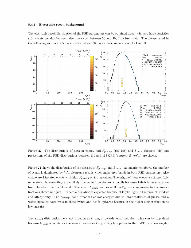
Figure 22: The distributions of data in energy and Fprompt (top left) and Lrecoil (bottom left) and
projections of the PSD-distributions between 110 and 115 QPE (approx. 15 keVee) are shown.
Figure 22 shows the distribution of the dataset in Fprompt and Lrecoil. As mentioned above, the number
of events is dominated by 39Ar electronic recoils which make up a bands in both PSD parameters. Also
visible are 4 isolated events with high Fprompt or Lrecoil-values. The origin of these events is still not fully
understood, however they are unlikely to emerge from electronic recoils because of their large separation
from the electronic recoil band. The mean Fprompt-values at 30 keVee are comparable to the singlet
fractions shown in figure 18 where a deviation is expected because of triplet light in the prompt window
and afterpulsing. The Fprompt-band broadens at low energies due to lower statistics of pulses and a
worse signal-to noise ratio in these events and bends upwards because of the higher singlet fraction at
low energies.
The Lrecoil distribution does not broaden as strongly towards lower energies. This can be explained
because Lrecoil accounts for the signal-to-noise ratio by giving late pulses in the PMT trace less weight.
37

The singlet fractions of electronic and nuclear recoils converge at low energies. Therefore, all photon
weights vanish here and the Lrecoil-mean at low energies converges towards 0.5.
It should be noted that the distribution is cut off at low Fprompt and low energies due to the trigger effi-
ciency: an event is only recorded when an (uncalibrated) threshold charge equivalent to approximately
20 QPE is exceeded value in a 177 ns time window. Because the peak intensity of an event is typically
reached in the prompt-window, this threshold charge is strongly correlated to the charge in the prompt
window and Fprompt of the event. Because the prompt window used by the trigger and Fprompt differ and
because Fprompt uses the SPE-corrected charge sum, this trigger effect is smeared out in Fprompt and Q.
As evident from the weight functions shown in the prior section, Lrecoil will also be higher for events with
a large prompt-charge fraction. Because electronic recoils typically have a lower peak-intensity they are
more affected by this effect than nuclear recoils at the same event energy such that it is ensured that
the detector is triggered for 100% of events in the WIMP search region.
An effective distribution that describes the 1D-projections of both distributions well over small energy
ranges is a gamma distribution convoluted with a Gaussian. The gamma distribution is defined with
the PDF f(x|µ, b) = 1bµΓ(b−1)
(xbµ
)(1/b−1)
exp(− xbµ ), where µ is the mean of the distribution and b is a
shape parameter. With the width of the Gaussian σ and a normalization constant Z the model has four
free parameters.
The right side of figure 22 shows the fit of the electronic recoil distributions in Fprompt and Lrecoil. The fit
interval is selected such that 100% trigger efficiency is reached at the lower fit limit. Because the trigger
efficiency curve in Lrecoil has not been calculated yet, it is assumed that the 100 % trigger efficiency
is reached at the same quantile in Fprompt and Lrecoil PSD parameters and the lower fit range is set
accordingly. Otherwise, this model describes the distributions well with a χ2/ndf = 68.54/67 for the
Fprompt and 35.87/53 for the Lrecoil distribution.
5.4.2 Signal
In order to estimate the position of the nuclear recoil band, the neutron calibration data can be used.
Figure 23 shows the distribution of the calibration data in Fprompt and energy. The event rate is still
dominated by 39Ar electronic recoils, however in addition to the dataset shown above, a second band at
higher Fprompt-values that corresponds to nuclear recoil events is visible. As discussed above, these are
not the only type of events that are produced by the neutron source. For example, the neutron source
also emits 4.4 MeV-γ photons, which are also detected. While they scatter in the argon via electronic
recoils, they might produce event topologies very different from 39Ar events because the particle source
is located outside of the detector. For example they might scatter with an electron in the acryl which
produces fast Cherenkov light before entering. The resulting event type could be hard to separate from
a nuclear recoil in the liquid. Another event that differs but might be hard to distinguish from the
expected WIMP interaction are neutrons scattering multiple times in the argon.
38

1
10
210
310
QPE0 50 100 150 200
prom
ptF
0.0
0.2
0.4
0.6
0.8
1.0
)ee
Energy (keV
0 5 10 15 20 25 30
QPE0 50 100 150 200
prom
ptF
0.0
0.2
0.4
0.6
0.8
1.0
1−10
1
10
)ee
Energy (keV
0 5 10 15 20 25 30
1
10
210
310
QPE0 50 100 150 200
reco
ilL
0.0
0.2
0.4
0.6
0.8
1.0
)ee
Energy (keV
0 5 10 15 20 25 30
QPE0 50 100 150 200
reco
ilL
0.0
0.2
0.4
0.6
0.8
1.0
1−10
1
10
)ee
Energy (keV
0 5 10 15 20 25 30
Figure 23: The distribution of AmBe calibration source data (left) and simulated Ar-40 nuclear recoils
(right) in Fprompt (top) and Lrecoil (bottom) is shown. The AmBe runs used here have a duration of 12
hours.
Projections of the AmBe calibration data in Fprompt are shown and compared to a simulation of the
source components in figure 24. Above 140 QPE (18 keVee), the distribution in Fprompt can be rep-
resented by simulated neutrons and gammas. Of the simulated neutrons, a subpopulation at higher
Fprompt overlaps with a simulation of single scatter nuclear recoils. Therefore, according to the simu-
lation, neutron scatters in the argon can be selected using an Fprompt > 0.6-cut above 140 QPE. This
population is only partially representative of WIMP events as significant fraction of the neutrons scatter
multiple times in the argon.
At lower energies, the agreement between the AmBe-data and simulated nuclear recoils and gammas
becomes worse. A hypothetical population of Cherenkov events could potentially make up for the dif-
ference between data and simulation, as shown in in the top two plots of figure 24. This agreement
at the current state of the simulation can only be achieved by applying a different cut set on the
Cherenkov population than on the other populations. This underlines how difficult reconstruction and
extraction of WIMP-like events from the AmBe-calibration data is. Therefore, to estimate the position
of the nuclear recoil band at low energies, simulated Ar40 nuclear recoils are used in the following section.
39
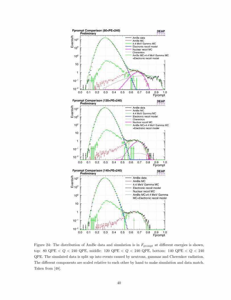
Figure 24: The distribution of AmBe data and simulation is in Fprompt at different energies is shown,
top: 80 QPE < Q < 240 QPE, middle: 120 QPE < Q < 240 QPE, bottom: 140 QPE < Q < 240
QPE. The simulated data is split up into events caused by neutrons, gammas and Cherenkov radiation.
The different components are scaled relative to each other by hand to make simulation and data match.
Taken from [48].
40

best case base case worst case
Singlet fraction rel. to SCENE + 0.01 0 - 0.01
Quenching factor rel. to SCENE + 0.01 0 - 0.01
Afterpulsing rate rel. to Calibration × 90% × 100 % × 110%
Dark noise rate per PMT (Hz) 400 500 600
Table 2: The input parameters used for the nuclear recoil simulation. The uncertainties of the SCENE-
parameters are the published systematical uncertainties. The uncertainties on the afterpulsing rate are
estimated from the analysis presented in appendix D. The dark rate and its uncertainty are estimated
using the pre-trigger window of pulse shapes (as in the fit described in appendix C).
To estimate the uncertainties on the position of the nuclear recoil band, the simulation is run two
additional times, using a optimistic scenario and pessimistic scenario. In the optimistic and pessimistic
scenario, the input-parameters listed in table 2 are set within their uncertainty such that PSD is expected
to improve and deteriorate, respectively.
5.4.3 Discrimination power
To make an informed decision which PSD parameter to use for dark matter search in DEAP-3600, their
ability to separate electronic recoils from the nuclear recoil band has to be quantified. A very simple
performance parameter can be defined as
δ =|µer − µnr|√σ2
er + σ2nr
. (33)
Here, µer, σer and µnr, σnr are mean and standard deviation in the electronic and nuclear recoil band,
respectively. This parameter therefore measures the separation of the two bands normalized by their
width.
µnr - µer
√σ2
nr + σ2er δ
Fprompt 0.366 0.079 4.64± 0.09
Lrecoil 0.294 0.062 4.72± 0.09
Table 3: δ for Fprompt and Lrecoil between 110 and 120 QPE. The uncertainties are calculated via the
standard error of the mean and variance.
Table 3 shows δ for the PSD parameters discussed in the prior section. The means of the electronic and
nuclear recoil distributions are closer together for the likelihood-based parameters than for the prompt-
window-based parameters. This can be explained by considering the shape of w(t) for both type of
discriminators: because w(t) for Fprompt is larger or equal w(t) for Lrecoil for all times except t > 10µs,
where only very few pulses are measured, Lrecoil overall uses less pulses to separate electronic and nuclear
41

recoils. This is however offset by a lower width of corresponding distributions. This is also consistent
with the statement above because many of the pulses that are discounted by Lrecoil are noise or after-
pulses, which broaden the PSD-distributions. As a result δ is slightly lower for the likelihood-based
parameter than for the prompt-window-based parameter.
While a big advantage of δ is that it does not assume the distributions to follow any model, it does not
necessarily measure the PSD-performance of the corresponding parameters. For example, tails in the
PSD-distributions that point away from the other population would increase the standard deviation and
therefore lower δ. As discussed in 1, backgrounds, even when predicted by a model, significantly impair
the sensitivity of the experiment. Therefore, in order to maximize its WIMP-sensitivity, DEAP-3600
has to achieve a background-free WIMP region of interest. This implies that the expected number of
electronic recoil events that ’leak’ into the nuclear recoil band over the lifetime of the detector is a
better measure of the PSD performance than δ. To estimate this number, we first quantify the position
of the WIMP search region in the given discrimination parameter. In all parameters considered here,
background events have a lower parameter value than signal events. We thus have to define a lower
bound of the signal region, called the signal threshold (ST). The position of the ST is defined based
on the quantile of signal events that falls above the ST. For a nuclear recoil acceptance (n.r.a.) of 90
%, the ST is set at the parameter value above which 90 % of the nuclear recoil events lie. Knowing
the shape of the discrimination parameter distribution for background events, we can now calculate
the probability that a background event will occur above the ST, which is equal to the quantile of the
electronic recoil distribution at this point. This probability will be referred to as the leakage probability
Pleak in the following section. In particular, the parameter value and nuclear recoil acceptance at a
leakage probability of 10−9 are evaluated. This number is chosen because with the high electronic
recoil background rate of approximately 107 events per year per PE-bin this corresponds to an expected
leakage past this point in the order of 10−2 per year. Because PSD improves exponentially towards
higher energies, this is an acceptable leakage probability at the lowest energy bin used for the dark
matter analysis, such that the leakage over the full WIMP search region stays in the order of 10−1, as
it will be shown below.
42

promptF0.35 0.40 0.45 0.50 0.55 0.60 0.65
leak
P
10−10
9−10
8−10
7−10
6−10
5−10
4−10
3−10
2−10
1−10
50%
n.r
.a.
90%
n.r
.a.
Model
Data
QPE80 100 120 140 160 180 200 220
prom
ptF
0.0
0.1
0.2
0.3
0.4
0.5
0.6
0.7
0.8
0.9
1.0
90% n.r.a.
leakage projection-910
)ee
Energy (keV
12 14 16 18 20 22 24 26 28
recoilL0.40 0.45 0.50 0.55 0.60 0.65
leak
P
10−10
9−10
8−10
7−10
6−10
5−10
4−10
3−10
2−10
1−10
50%
n.r.
a.
90%
n.r.
a.
Model
Data
QPE80 100 120 140 160 180 200 220
reco
ilL
0.0
0.1
0.2
0.3
0.4
0.5
0.6
0.7
0.8
0.9
1.0
90% n.r.a.
leakage projection-910
)ee
Energy (keV
12 14 16 18 20 22 24 26 28
Figure 25: Left: The leakage probability in 110 to 120 QPE as a function of the discrimination parameter
value. Right: The 10−9-leakage projection estimated from the electronic recoil distribution model. This
is compared to the 90 % nuclear recoil acceptance line obtained from Monte Carlo.
The leakage probability as a function of Fprompt and Lrecoil between 110 and 120 QPE is shown in figure
25 (left). The leakage estimates from data is the fraction of events that exceed the corresponding value of
the parameter and the uncertainties shown are the Wilson score interval [49], which is an approximation
for the uncertainties on estimates of binomial probabilities. Because the dataset used contains 5 · 107
events, the lowest leakage probability that can be estimated directly from data is (5 · 107)−1 = 2 · 10−8.
To obtain lower leakage probabilities, the model that was fit to the electronic recoil background in figure
22 is extrapolated into the lower leakage probability-region. The estimated Pleak in model and data
agree within the Wilson score intervals. Using the model-estimate the leakage probabilities at the 90
% quantile of the nuclear recoil acceptance (n.r.a.), as well as the Fprompt and Lrecoil-values and 10−9
leakage probabilities can be calculated. The positions of the parameter values at which 10−9 projected
leakage probability is reached is shown as a function of energy on right of figure 25. These estimates
are obtained over energy bins of 10 QPE (80 to 90 QPE, 90 to 100 QPE..). The uncertainties on the
leakage position are obtained using the uncertainties of the fit parameters and are calculated using a
Monte Carlo simulation, where upon each iterations fit parameters are randomly drawn from Gaussian
distributions with mean and width determined by the fit. The uncertainty shown is the standard devi-
ation of the distribution obtained this way. To put the achieved leakage into perspective relative to the
nuclear recoil distribution, the 90 % n.r.a. line is also shown. Here, the uncertainties are calculated by
43
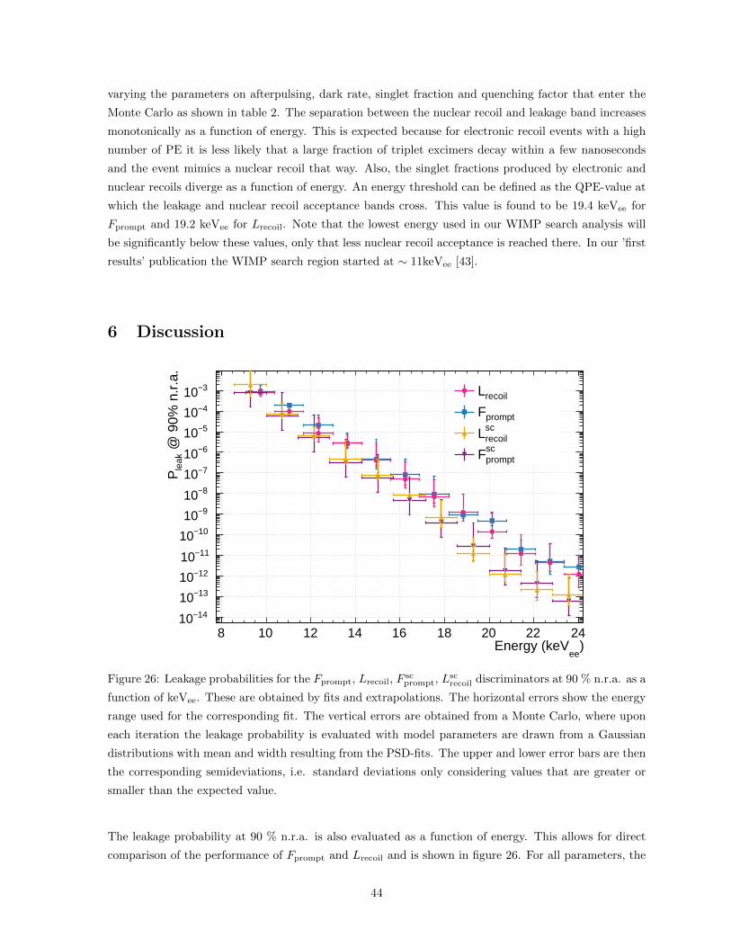
varying the parameters on afterpulsing, dark rate, singlet fraction and quenching factor that enter the
Monte Carlo as shown in table 2. The separation between the nuclear recoil and leakage band increases
monotonically as a function of energy. This is expected because for electronic recoil events with a high
number of PE it is less likely that a large fraction of triplet excimers decay within a few nanoseconds
and the event mimics a nuclear recoil that way. Also, the singlet fractions produced by electronic and
nuclear recoils diverge as a function of energy. An energy threshold can be defined as the QPE-value at
which the leakage and nuclear recoil acceptance bands cross. This value is found to be 19.4 keVee for
Fprompt and 19.2 keVee for Lrecoil. Note that the lowest energy used in our WIMP search analysis will
be significantly below these values, only that less nuclear recoil acceptance is reached there. In our ’first
results’ publication the WIMP search region started at ∼ 11keVee [43].
6 Discussion
)ee
Energy (keV8 10 12 14 16 18 20 22 24
@ 9
0% n
.r.a
.le
akP
14−10
13−10
12−10
11−10
10−10
9−10
8−10
7−10
6−10
5−10
4−10
3−10 recoilL
promptF
recoilscL
promptscF
Figure 26: Leakage probabilities for the Fprompt, Lrecoil, Fscprompt, L
screcoil discriminators at 90 % n.r.a. as a
function of keVee. These are obtained by fits and extrapolations. The horizontal errors show the energy
range used for the corresponding fit. The vertical errors are obtained from a Monte Carlo, where upon
each iteration the leakage probability is evaluated with model parameters are drawn from a Gaussian
distributions with mean and width resulting from the PSD-fits. The upper and lower error bars are then
the corresponding semideviations, i.e. standard deviations only considering values that are greater or
smaller than the expected value.
The leakage probability at 90 % n.r.a. is also evaluated as a function of energy. This allows for direct
comparison of the performance of Fprompt and Lrecoil and is shown in figure 26. For all parameters, the
44

PSD performance improves exponentially by an order of magnitude per 15 keVee.
δ Pleak at 90 % n.r.a. Energy threshold in keVee
Fprompt 4.64± 0.09 4.5 · 10−7(+2.6 · 10−7/− 4.2 · 10−8) 19.4± 1.7
Lrecoil 4.72± 0.09 3.4 · 10−7(+3.4 · 10−7/− 8.2 · 10−8) 19.2± 1.9
F scprompt 5.53± 0.11 4.8 · 10−8(+8.8 · 10−8/− 5.4 · 10−9) 17.5± 2.0
Lscrecoil 5.47± 0.11 6.5 · 10−8(+1.0 · 10−7/− 6.7 · 10−9) 18.0± 1.7
Table 4: Separation (δ), leakage and energy threshold for various discriminators. Pleak and δ are evalu-
ated between (14.3± 0.4) keVee (110 QPE or 100 NSC) and (15.6± 0.4) keVee (120 QPE or 109 NSC).
The energy thresholds are obtained by fitting exponentials to the leakage probabilities shown in figure
26. The energy threshold is then the energy at which the fit function crosses the 10−9 leakage-probability
line. The errors are the standard deviations of the energy threshold distributions obtained by varying
the fit parameters within their uncertainties. Uncertainties from the light yield are not considered here.
The performance of all PSD parameters that were investigated in this work is summarized in table 4.
The discriminators using nnsc perform significantly better than the corresponding version using charge.
This implies that indeed the reduction of afterpulsing and SPE-noise strongly benefits PSD. Within the
discriminators using the same photon-estimate, the likelihood-based discriminators and prompt-window-
based discriminators demonstrate very comparable PSD performance. This is expected because as shown
in figure 19, the photon weights used by both discriminator types are very similar in the first 5 µs, where
90 % of the pulses are detected.
The Lrecoil appears to perform slightly better than Fprompt. This indicates that the discounting of pulses
that are measured at times where afterpulsing and other noise components are dominant improves PSD.
When comparing Lscrecoil and F sc
prompt, the opposite trend is observed: here the prompt-window-based dis-
criminator performs slightly better than the likelihood-based version. This is surprising because accord-
ing to the Neyman-Pearson Lemma, the likelihood ratio should be the better discriminator. One reason
for the superior performance of the prompt-window-based discriminators could be that for evaluation
of the likelihood, an approximation is used in Lrecoil, where the pulses are assumed to be independent.
While this assumption holds for argon scintillation and dark noise, it does not for afterpulsing, where
pulses are directly caused by other pulses. Because Lscrecoil and F sc
prompt use the afterpulsing-corrected
photon count nnsc, this approximation should be valid for these parameters and can not explain this
difference. Another possible explanation could be the comparison of distributions in data and Monte
Carlo that was done to obtain the PSD performance measures. Because the likelihood-based parame-
ters rely on the exact timing information, they could be more affected by mismatches between Monte
Carlo and data. For example, because all afterpulsing falls into the late window, Fprompt is only sen-
sitive to the afterpulsing rate, whereas Lrecoil is sensitive to the precise timing distribution of afterpulsing.
One component that has been found to differ in data and Monte Carlo and strongly affects the average
pulse shape is given by delayed TPB light reemission. In figure 19 it was shown that delayed TPB
45

fluorescence has an impact on the photon weights, such that the information carried by photons emit-
ted between 200 and 4000 ns decreases. Generally, delayed light TPB will be harmful to PSD because
re-emitted delayed photons effectively lose their timing information.
In DEAP, the delayed TPB light emission is hard to extract from the electronic recoil data because
here, the late light is dominated by the triplet component. By comparison of pulse shape-fits described
in appendix C using models with and without delayed TPB fluorescence it can be concluded that this
component is likely also seen in DEAP. Here, it was found that with the χ2 of fits including the TPB
model measured by Segreto et al [38] is significantly lower than the χ2 of fits without this component.
Note that the TPB fluorescence parameters are fixed to their published values such that no additional
parameters are added. At the same time, no TPB fluorescence model is currently implemented in Monte
Carlo. The Segreto paper uses a combination of different exponentials to represent the TPB fluorescence
pulse shape. Another measurement has become available in late 2017 and is compared to the effective
model that is used by Segreto in figure 27. Here, a more complicated model is used that assumed that
the delayed fluorescence is produced by the decay of triplet states. Because these triplet states have a
non-luminous deexcitation channel, the time structure of their decay rate does not follow an exponential.
While the two measurements agree in the order of magnitudes of the measured intensities, the lifetime
measured by the Princeton group appears to be significantly lower. Differences in the two measurements
include the thickness of the TPB layer which is 1000 µg cm−2 in the E. Segreto and 265 µg cm−2 in the
C. Stanford measurement. The estimated thickness of the TPB layer in DEAP is: 300 µg cm−2) [30].
Time (ns)500 1000 1500 2000 2500
)-1
Rel
ativ
e in
tens
ity (
ns
5−10
4−10
3−10
E. Segreto et al
C. Stanford et al
Figure 27: TPB fluorescence trace measured by E. Segreto et al [38] and C. Stanford et al [39]. Both
measurements of the TPB response to argon UV photons are obtained by reducing the argon scintillation
time structure to a delta-like peak by contaminating the argon with nitrogen.
46
While it would be good to understand the discrepancies of the two measurements in the future, the
Princeton measurement is scheduled to be implemented in the DEAP detector Monte Carlo. This is a
necessity to get a better estimate on the position of the nuclear recoil band regardless of which PSD
parameter is chosen for a future dark matter analysis. The fraction of delayed photons will cause a
shift an Fprompt whereas Lrecoil will be sensitive to the precise structure of the TPB fluorescence pulse
shape. It will be interesting to repeat the PSD analysis under the new Monte Carlo to see whether TPB
fluorescence plays a role in the underperformance of Lscrecoil.
It should also be mentioned here that while using Monte Carlo (MC) to obtain the signal position in
Fprompt can be justified with the good agreement of the Fprompt distributions for AmBe-calibration and
Monte Carlo, the same comparison between data and MC has not been done yet for Lrecoil. It could
be the case that the agreement is worse here than for Fprompt for the reasons named above. Therefore,
comparing the Lrecoil distributions in Monte Carlo and data might be misleading. This hypothesis can
be tested by using a electronic recoil Monte Carlo instead of the 39Ar-background data. If the un-
derperformance of Lscrecoil is indeed due to mismatches in data and MC, the parameter should perform
better when its simulated nuclear recoil distribution is compared against the simulated electronic recoil
distribution. For the electronic recoil simulation, electrons with flat momentum distribution between 5
keV and 50 keV are simulated homogeneously distributed in the liquid. It is found that when comparing
MC with MC, the δ-separation parameter for F scprompt and Lsc
recoil coincide, whereas δ is lower for Lscrecoil
when comparing data to MC as shown in table 4. This means that indeed mismatches between data and
Monte Carlo play a role in the poor performance of Lscrecoil. δ is used as the PSD performance measure
here because it does not require the high statistics in the electronic recoil band that are required for
the model fit. This is convenient when using simulated electronic recoils as the simulation is highly
CPU-intensive. Despite the weaknesses of δ, it is a very good predictor of the other PSD performance
measures as shown in table 4.
As shown in appendix C, the argon triplet lifetime changes over time. This means that in principle,
the PDFs used to build the photon weight functions would have to be adjusted after certain periods
of times or otherwise the PSD performance achieved by the likelihood-based discriminators might de-
teriorate as the PDFs start diverging from the pulse shapes. In order to estimate how sensitive Lrecoil
is to mismatches between the PDFs and the pulseshapes, the PSD performance of Lrecoil is evaluated
using PDFs which differ from data. Here, an increase and decrease of the triplet lifetime of 50 ns is
used, which is double the change that was found in appendix C over one year. The resulting change in
δ is found to be < 0.01, which suggests that the PDFs are robust against the detector changes that are
expected in DEAP-3600.
Finally, the procedure used to evaluate the leakage probabilities has a few weaknesses. For example, an
effective model is used to fit the PSD-distributions. While the agreement between model and data is
excellent, in principle there is no physical reason why the model should be representative of the ’real
leakage’ when extrapolated over the several order of magnitude. For Fprompt, it has been shown in [44]
47

that the distribution can be described by physically motivated model. This is done by calculating the
probability that a pulse is a prompt pulse taking into account among others the singlet fractions, ar-
gon scintillation time structure, dark noise, SPE-charge distribution and afterpulsing probabilities. A
full physics model for the distribution of the prompt-window-based parameters in DEAP-3600 is under
development. With regard to a physical model of the Lrecoil-distribution, knowing the probability that
a pulse is a prompt or late pulse is not sufficient to describe the distribution of Lrecoil as Lrecoil takes
into account the exact timing information of each pulse. Therefore, the physical model distribution of
likelihood-based discriminators is much more complicated and can also not be evaluated analytically.
Distributions would in this case have to built from Monte Carlo which is an additional disadvantage of
likelihood-based discrimination against prompt-window-based discrimination.
7 Conclusion and Outlook
DEAP-3600 is a single-phase liquid argon dark matter detector. The largest background, with more
than 109 events in the preliminary energy region of interest of 15 to 30 keVee for the planned exposure,
is the beta decay of 39Ar. Pulse shape discrimination is used to discriminate this electron-recoil type
background from the nuclear recoil events we expect WIMP recoils to induce. PSD in LAr is based on
two effects: Scintillation light is emitted from a singlet and a triplet excimer with a 2 order of magnitude
lifetime difference, and the fraction of each excimer that is excited depends on the type of interaction.
PSD thus boils down to estimating the fraction of singlet and triplet excimers as accurately as possible
for each event. At the low energies where WIMP scattering events are expected to occur, less than 300
photons are detected per event. The statistical variations in photon arrival time for such a small number
of photons make PSD challenging.
The goal of this work was to implement and compare the performance of different PSD parameters.
Pulse shape discrimination is predicated on an understanding of the time structure of a typical event.
Therefore, the average pulse shape for 39Ar beta-decays was studied in detail. Since Ar-39 beta decay
is the main background in DEAP-3600, a large number of sample events was available for analysis. It
showed that the detector response function, dominated by PMT afterpulsing, dark noise, and delayed
light emission of the wavelength shifter TPB, has a significant impact on the measured pulse shapes.
DEAP currently uses a simple ”prompt photon” based PSD method. This method does not make use
of the full information collected for each event, and does not attempt to account for the known detector
response function. Including more of the available information about the detector response starts at
the photon counting level. The standard estimator uses photons counted by the charge method: The
charge of each PMT pulse is divided by the mean single-photoelectron charge to estimate the number
of photo electrons and thus the number of photons that arrived at the time of each pulse. A second
48
existing estimator attempts to remove the known parts of the detector response function. It determines
the most likely number of photons in a PMT pulse, based on the known arrival time of the pulse, the
LAr scintillation PDF, and the afterpulsing PDF, which is known from PMT calibration. I found that
this estimator creates a biased pulse shape. The source of this bias was investigated and the estimator
was modified to eliminate the bias. The different photon counting methods yield two prompt-based
discriminators: Fprompt, the most naive estimator, and F scprompt, which uses a photon count that includes
information about the detector response and LAr scintillation physics.
In addition to or conjunction with basing the PSD discriminator on a better estimate for the photon
count, additional information can be included in the PSD method itself. A likelihood-based discrimi-
nator based on [47] was developed, which makes use of the full photon timing information available in
an event. Unlike prompt-based discriminators, likelihood discriminators require pulse shape PDFs for
signal and background. These are used to determine how likely it is that the photon timing distribution
of a given event matches the signal or background distribution. Different ways to produce such PDFs,
including basing them on measured data, on Monte Carlo detector simulation, and on mathematical
models, are explored and discussed. I found that background and signal PDFs based on a mathematical
description informed by measured pulse shapes works best. The two different photon counting methods
again yield two likelihood-based discriminators: Lrecoil and Lscrecoil.
The new likelihood discriminator assigns a weight to each detected photon based on the photon arrival
time. I showed how these weights are calculated based on the signal and background PDFs. In order
to compare this method to the existing prompt-based method, equivalent weights for the prompt-based
estimator were derived. In order to further compare the PSD power of the simple charge-based photon
counting method to the more advanced probabilistic photon estimation method, the definition of the
weights was extended for non-integer estimates of the photon count.
The likelihood weights are a measure for how much information is contained in a photon arriving at a
given time. The influence of the detector response and the photon counting method is illustrated based
on these weights. This is a novel way to determine the influence of detector response on the PSD power
and to compare PSD methods.
The performance of each PSD estimator was evaluated by comparing the event energy (that is the num-
ber of detected photons) at which the probability to find a background event in the signal region is 10−9
or smaller. The signal region is defined such that the signal-acceptance is 90 %. The position of the
signal region and its uncertainties are evaluated here using detector Monte Carlo simulation. A second,
equivalent measure, used here is the leakage probability at 15 keVee.
The performance of PSD discriminators that use the likelihood-based photon count is significantly better
than the same discriminator using the charge-based photon count. This shows that afterpulsing and
49

the uncertainty on how many photons are in a PMT pulse degrade PSD performance, and that this
degradation can be mitigated by better analysis techniques.
The likelihood-based PSD method using charge performs only slightly better than the equivalent prompt-
window based discriminator, whereas the likelihood based method using the Bayesian photon count
performs slightly worse. This result does not stem from any weakness of the likelihood algorithm imple-
mented here, but is a consequence of liquid argon scintillation physics. Study of the likelihood weights
shows that the prompt-based discriminator’s equivalent weights are already close to optimal. This can
be understood by considering the large difference between the argon excimer lifetimes. At any given
pule time, one of the two excimers strongly dominates the scintillation PDF, so that the photon infor-
mation content as a function of time approximates a step-function, which is captured adequately by the
prompt-based discriminator.
This result also shows that removing detector effects at the level of photon counting is better than
including detector effects in the likelihood function. Any advantage of the likelihood-based over the
prompt-based discriminator, for the same photon counting method, comes from its better handling of
detector effects. Use of the Bayesian photon count in a prompt-based PSD method already mitigates
detector effects sufficiently. The difference between prompt and likelihood-based PSD methods might be
larger for scintillators where the scintillation response can not be so cleanly divided into two components,
such as the BC-501 liquid scintillator [50].
I conclude by recommending F scprompt as the PSD-parameter to use for dark matter search in DEAP-
3600, because this parameter conserves the useful analytical properties of a prompt-based discriminator
while achieving an excellent PSD result. This is under the assumption that an energy calibration for the
Bayesian photon is unproblematic, which has not been verified yet. Also, the simulation which DEAP
relies on to estimate its signal distribution should be improved by implementing a TPB fluorescence
model.
50

Appendix
A Data selection
This work is focused on the electronic recoil liquid argon scintillation background in DEAP-3600, so
data cuts are established which select these events. Other event types that are seen by the detector are
introduced in section 3.4. Below, all cut variables and values that are applied to all data presented in
this work can be found. These cuts are equivalent to the cuts that were used for the published dark
matter analysis paper [43].
Low-level cuts Events that show behaviour of the electronics or where the DAQ-software was run
under a setup unsuitable to detect physics events are removed.
These includes the following cases:
• a digitzer has a bad baseline
• a digitizer was saturated
• event is close to pulse-test-event
• an unconnected channel measures a pulse
• the DAQ is too busy to read out digitizers
• trigger/digitizers are out of sync
• the charge integral of a pulse is truncated
Event position Another population of events observed by DEAP-3600 are so-called surface events,
i.e. events that arise from the decay of radioactive material on the surface of the acrylic cryostat. These
events can produce a WIMP-like signal when a daughter nucleus of an alpha decay is pushed into the
liquid argon, where it scatters in a nuclear recoil. Because this scatter occurs close to the detector
surface, these events can be removed by cutting events with features that are typical for surface events.
Two variables are used in this work to remove events that likely come from the edges of the detector: the
fraction of charge and the fraction of estimated photons nnsc seen by the PMT which saw most charge
and nnsc during the event, respectively. The cut values used are > 20% and > 7%. These cuts also
effectively remove Cherenkov events, where typically only very few PMTs see a short light flash.
Pile-up cuts For each event, approximately 2.5 us of PMT traces before the trigger time are recorded.
NHitsEarly is the number of pulses in the first 1.6 us in this pre-trigger window. This cut removes pile-up
events and events that overlap with a long-lifetime component of a prior event. The cut value used is 3.
Additionally, only events are considered which were triggered 20 µs after the last event was triggered or
51

more.
Also, sophisticated algorithms are implemented which spot and remove pile-up events by looking at their
time structure.
B PE counting and afterpulsing removal
Afterpulsing complicates the event reconstruction in various ways. For example, it worsens the energy
resolution by adding noise to the pulse shape. This also lowers the pulse shape discrimination power that
can be achieved. Additionally, afterpulsing can distort the charge distribution across the PMT array and
therefore complicates reconstruction of the event position. Through a model of the argon scintillation
and the afterpulsing response an algorithm can be implemented which removes or underweights pulses
that are likely afterpulses. This is realized by performing a Bayesian analysis for each pulse [51]:
p(nsc + nap = npe|Q) = p(Q|npe)/p(Q)p(nsc + nap = npe). (34)
Here, nsc is the number of photons that caused the pulse and nap is an integer measure for the afterpulsing
charge in units of the SPE-charge. Because the charge of afterpulsing and scintillation is indistinguish-
able, an informative prior p(nsc + nap = npe) is constructed to evaluate the probability of either using
the scintillation and afterpulsing physics in the experiment. The posterior p(nsc + nap = npe|Q) is then
used to give an estimate of the number of photons and afterpulsing that caused the pulse. In addition to
removing afterpulsing, this estimate could potentially reduce the noise that is introduced by the broad
charge-distribution that is produced by a discrete number of photons.
The number of photons seen by a PMT during the full event can then be estimated as the sum over the
estimated number of non-afterpulses in each pulse seen by this PMT. This value summed over all PMTs
gives an estimate of the total photons in an event nevsc .
B.1 Evaluating the prior
Priors are generally used to incorporate prior knowledge into a parameter estimate. In this case, this is
the prompt fraction of light (i.e. Fprompt in equation 17) of the event and the total charge observed by
the PMT looked at during the event npmtq .
Pulses, especially when consisting of multiple subpulses, can span over a length of > 100 ns. This means
that a pulse could contain an afterpulse which was caused by a subpulse of the same pulse. This inter-
dependence is neglected in this analysis as the afterpulsing and scintillation probabilities within a pulse
are treated independently, such that p(nsc + nap = npe) = p(nsc)p(nap).
The theoretical argon scintillation probability distribution function (PDF) combines a flat dark noise
52
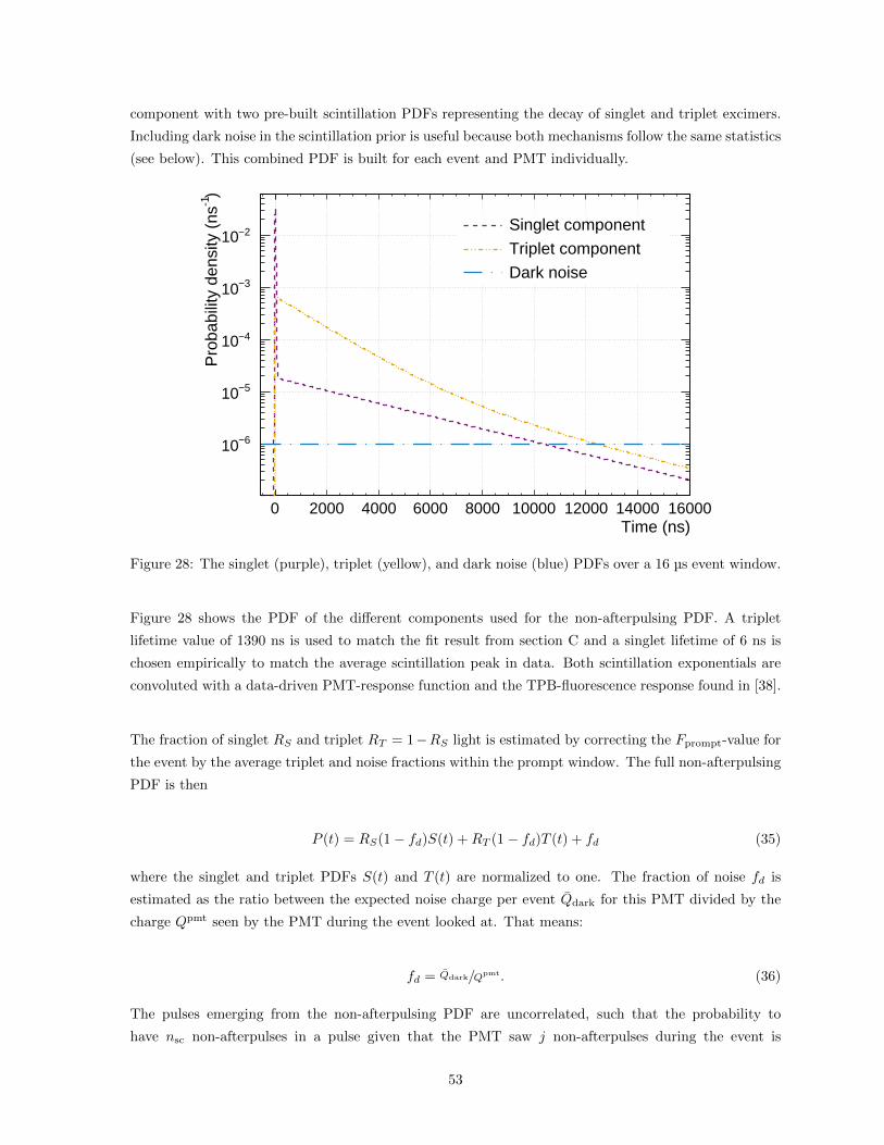
component with two pre-built scintillation PDFs representing the decay of singlet and triplet excimers.
Including dark noise in the scintillation prior is useful because both mechanisms follow the same statistics
(see below). This combined PDF is built for each event and PMT individually.
Time (ns)0 2000 4000 6000 8000 10000 12000 14000 16000
)-1
Pro
babi
lity
dens
ity (
ns
6−10
5−10
4−10
3−10
2−10Singlet component
Triplet component
Dark noise
Figure 28: The singlet (purple), triplet (yellow), and dark noise (blue) PDFs over a 16 µs event window.
Figure 28 shows the PDF of the different components used for the non-afterpulsing PDF. A triplet
lifetime value of 1390 ns is used to match the fit result from section C and a singlet lifetime of 6 ns is
chosen empirically to match the average scintillation peak in data. Both scintillation exponentials are
convoluted with a data-driven PMT-response function and the TPB-fluorescence response found in [38].
The fraction of singlet RS and triplet RT = 1−RS light is estimated by correcting the Fprompt-value for
the event by the average triplet and noise fractions within the prompt window. The full non-afterpulsing
PDF is then
P (t) = RS(1− fd)S(t) +RT (1− fd)T (t) + fd (35)
where the singlet and triplet PDFs S(t) and T (t) are normalized to one. The fraction of noise fd is
estimated as the ratio between the expected noise charge per event Qdark for this PMT divided by the
charge Qpmt seen by the PMT during the event looked at. That means:
fd = Qdark/Qpmt. (36)
The pulses emerging from the non-afterpulsing PDF are uncorrelated, such that the probability to
have nsc non-afterpulses in a pulse given that the PMT saw j non-afterpulses during the event is
53
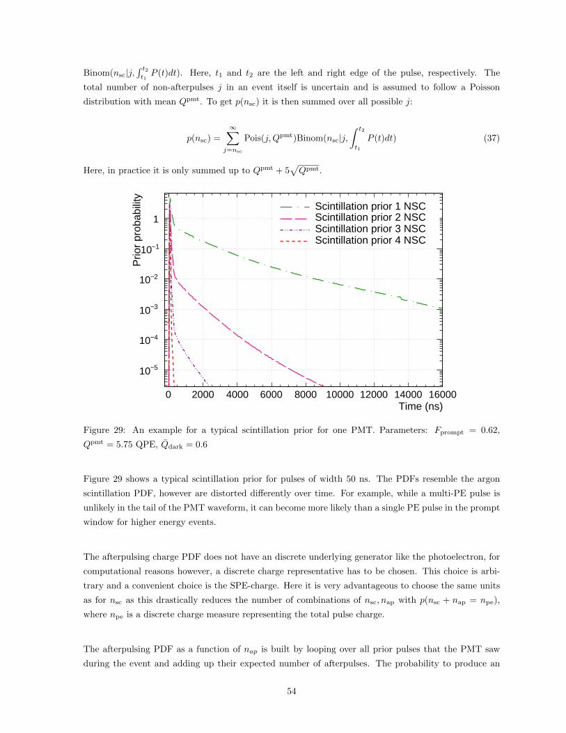
Binom(nsc|j,∫ t2t1P (t)dt). Here, t1 and t2 are the left and right edge of the pulse, respectively. The
total number of non-afterpulses j in an event itself is uncertain and is assumed to follow a Poisson
distribution with mean Qpmt. To get p(nsc) it is then summed over all possible j:
p(nsc) =
∞∑j=nsc
Pois(j,Qpmt)Binom(nsc|j,∫ t2
t1
P (t)dt) (37)
Here, in practice it is only summed up to Qpmt + 5√Qpmt.
Time (ns)0 2000 4000 6000 8000 10000 12000 14000 16000
Prio
r pr
obab
ility
5−10
4−10
3−10
2−10
1−10
1Scintillation prior 1 NSCScintillation prior 2 NSCScintillation prior 3 NSCScintillation prior 4 NSC
Figure 29: An example for a typical scintillation prior for one PMT. Parameters: Fprompt = 0.62,
Qpmt = 5.75 QPE, Qdark = 0.6
Figure 29 shows a typical scintillation prior for pulses of width 50 ns. The PDFs resemble the argon
scintillation PDF, however are distorted differently over time. For example, while a multi-PE pulse is
unlikely in the tail of the PMT waveform, it can become more likely than a single PE pulse in the prompt
window for higher energy events.
The afterpulsing charge PDF does not have an discrete underlying generator like the photoelectron, for
computational reasons however, a discrete charge representative has to be chosen. This choice is arbi-
trary and a convenient choice is the SPE-charge. Here it is very advantageous to choose the same units
as for nsc as this drastically reduces the number of combinations of nsc, nap with p(nsc + nap = npe),
where npe is a discrete charge measure representing the total pulse charge.
The afterpulsing PDF as a function of nap is built by looping over all prior pulses that the PMT saw
during the event and adding up their expected number of afterpulses. The probability to produce an
54

afterpulse f(Qi)F (δti , nap) with a certain delay after an initial pulse and of charge equivalent to nap
can be taken from the histogram shown in figure 6. The expected number of afterpulses observed scales
linearly with the charge of the initial pulse f(Qi) = a+ bQi, where a and b were determined separately
for each PMT using the calibration measurement (see [32]).
p(nap) = 1− exp
Nprev∑i=1
f(Qi)F (δti, nap)
(38)
Formula 38 shows the Poisson probability that > 0 afterpulses of nap charge equivalent are observed.
Here, Nprev is the number of prior pulses. The possibility of the pulse being produced by two or more
afterpulses caused by different prior pulses is ignored here.
Time (ns)0 2000 4000 6000 8000 10000 12000 14000 16000
Prio
r pr
obab
ility
6−10
5−10
4−10
3−10
Afterpulsing prior 1 NAPAfterpulsing prior 2 NAPAfterpulsing prior 3 NAPAfterpulsing prior 4 NAP
Figure 30: An example for a typical afterpulsing prior.
Figure 30 shows a typical afterpulsing prior for pulses of width 50 ns. Here, as for nnsc in the scintillation
prior, the prior tends to decrease with the amount of charge attributed to afterpulsing, however this
effect is less pronounced here. This means that high-charge pulses, especially when late in the PMT
trace, are likely afterpulses.
B.2 Evaluating the likelihood
The charge response to a discrete number of PE npe = nsc + nap, p(Q|npe), is modelled as part of the
SPE calibration (see figure 5). To obtain the n-PE charge distribution the SPE charge distribution is
convoluted with itself n times.
55
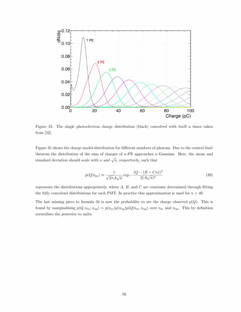
Figure 31: The single photoelectron charge distribution (black) convolved with itself n times taken
from [52].
Figure 31 shows the charge model-distribution for different numbers of photons. Due to the central limit
theorem the distribution of the sum of charges of n-PE approaches a Gaussian. Here, the mean and
standard deviation should scale with n and√n, respectively, such that
p(Q|npe) ≈ 1√2πA√n
exp− (Q− (B + Cn))2
2(A√n)2
(39)
represents the distributions appropriately, where A, B, and C are constants determined through fitting
the fully convolved distributions for each PMT. In practice this approximation is used for n > 40.
The last missing piece to formula 34 is now the probability to see the charge observed p(Q). This is
found by marginalising p(Q,nsc, nap) = p(nsc)p(nap)p(Q|nsc, nap) over nsc and nap. This by definition
normalises the posterior to unity.
56
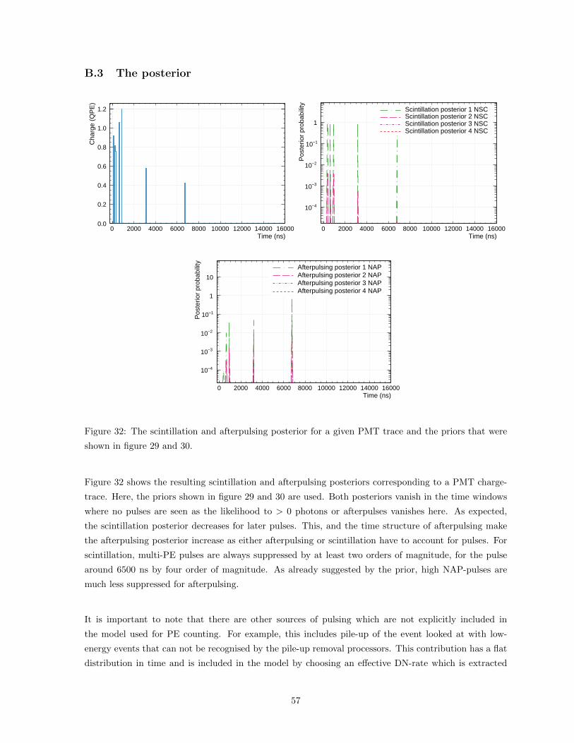
B.3 The posterior
Time (ns)0 2000 4000 6000 8000 10000 12000 14000 16000
Cha
rge
(QP
E)
0.0
0.2
0.4
0.6
0.8
1.0
1.2
Time (ns)0 2000 4000 6000 8000 10000 12000 14000 16000
Pos
terio
r pr
obab
ility
4−10
3−10
2−10
1−10
1
Scintillation posterior 1 NSCScintillation posterior 2 NSCScintillation posterior 3 NSCScintillation posterior 4 NSC
Time (ns)0 2000 4000 6000 8000 10000 12000 14000 16000
Pos
terio
r pr
obab
ility
4−10
3−10
2−10
1−10
1
10
Afterpulsing posterior 1 NAPAfterpulsing posterior 2 NAPAfterpulsing posterior 3 NAPAfterpulsing posterior 4 NAP
Figure 32: The scintillation and afterpulsing posterior for a given PMT trace and the priors that were
shown in figure 29 and 30.
Figure 32 shows the resulting scintillation and afterpulsing posteriors corresponding to a PMT charge-
trace. Here, the priors shown in figure 29 and 30 are used. Both posteriors vanish in the time windows
where no pulses are seen as the likelihood to > 0 photons or afterpulses vanishes here. As expected,
the scintillation posterior decreases for later pulses. This, and the time structure of afterpulsing make
the afterpulsing posterior increase as either afterpulsing or scintillation have to account for pulses. For
scintillation, multi-PE pulses are always suppressed by at least two orders of magnitude, for the pulse
around 6500 ns by four order of magnitude. As already suggested by the prior, high NAP-pulses are
much less suppressed for afterpulsing.
It is important to note that there are other sources of pulsing which are not explicitly included in
the model used for PE counting. For example, this includes pile-up of the event looked at with low-
energy events that can not be recognised by the pile-up removal processors. This contribution has a flat
distribution in time and is included in the model by choosing an effective DN-rate which is extracted
57

in-situ. Here, but especially in the case of pile-up with Cherenkov light, pulses are not uncorrelated
anymore as multi-PE flashes are seen by only a few PMTs in a very short time window. It has not yet
been investigated how the PE counting algorithm handles such event topologies, which explicitly do not
follow the physical model used by the priors.
B.4 Parameter estimation and validation
Two very prominent estimators in Bayesian statistics are the maximum a posteriori (MAP) estimator
and Minimum Mean Square Error (MMSE) estimator. Parameters in the MAP-framework are estimated
as the most likely values given the data observed, i.e. the mode of the posterior. Common criticism
of this estimator includes that the mode is generally not representative of the entire posterior. The
MMSE estimate minimizes the mean squared difference between the parameter and estimator. It can
be shown that this is that this equivalent to setting the estimate to its mean over the posterior. This
by definition makes the MMSE estimator mean-unbiased under the condition that the model chosen
describes the data [53]. A downside of the MMSE-method is that the evaluation of the posterior mean
can be computationally very expensive, in particular for posteriors of multiple continuous variables.
In this section the MAP and MMSE estimator are applied and discussed in the context of the afterpulsing-
removal-problem.
The MAP-estimates npe, nsc and nap are chosen such that the posterior p(nsc + nap = npe|Q) is a
maximized.
In the MMSE approach, the estimate is the parameter mean over the posterior. Here, the integration is
not computationally costly as there are only two discrete random variables (nsc and nap):
nsc =
nmaxpe∑
npe=0
∑nsc,nsc withnsc+nap=npe
nscp(nsc + nap = npe|Q) (40)
, where nmaxpe = nq + 5
√nq. Note that npe, nsc and nap do not necessarily take integer values in this
case.
58

Figure 33: Distributions of the npe, nsc and nap estimates using the MAP and MMSE estimator. The
npe distribution is also compared with the normalized charge distribution, which, like npe, includes
scintillation and afterpulsing.
The frequencies of npe, npe, npe using the two different estimators, as well as the normalized charge dis-
tribution is shown in figure 33. As the MAP estimates can only take integer values, their distributions
are series of delta-peaks. The nsc distribution is highly concentrated at the 1 nsc with approximately 80
% of pulses taking this value. 8 % of pulses have a 0 nsc which coincides notably well with the average
afterpulsing rate across the PMT array. The MMSE estimate of nsc can take non-integer values, however
its distribution is still peaked at lower nsc integer values. The nap-distributions are fairly flat towards
higher nap. This is consistent with the calibration as indicated by the afterpulsing prior.
L1 = |nsc − nphotons| (41)
L2 = (nsc − nphotons)2 (42)
L0 =
0 if nsc = nphotons
1 otherwise(43)
One good way to evaluate the accuracy of the nnsc photons estimators, is to calculate their performance
under different loss functions. Two sensible loss functions are for example the L1 and L2 deviations
59
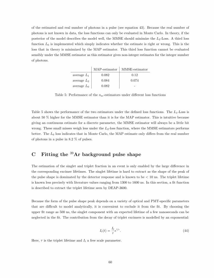
of the estimated and real number of photons in a pulse (see equation 43). Because the real number of
photons is not known in data, the loss functions can only be evaluated in Monte Carlo. In theory, if the
posterior of the model describes the model well, the MMSE should minimize the L2-Loss. A third loss
function L0 is implemented which simply indicates whether the estimate is right or wrong. This is the
loss that in theory is minimized by the MAP estimator. This third loss function cannot be evaluated
sensibly under the MMSE estimator as this estimator gives non-integer estimates for the integer number
of photons.
MAP-estimator MMSE-estimator
average L1 0.082 0.12
average L2 0.084 0.074
average L0 0.082 -
Table 5: Performance of the nsc-estimators under different loss functions
Table 5 shows the performance of the two estimators under the defined loss functions. The L1-Loss is
about 50 % higher for the MMSE estimator than it is for the MAP estimator. This is intuitive because
giving an continuous estimate for a discrete parameter, the MMSE estimator will always be a little bit
wrong. These small misses weigh less under the L2-loss function, where the MMSE estimators performs
better. The L0 loss indicates that in Monte Carlo, the MAP estimate only differs from the real number
of photons in a pulse in 8.2 % of pulses.
C Fitting the 39Ar background pulse shape
The estimation of the singlet and triplet fraction in an event is only enabled by the large difference in
the corresponding excimer lifetimes. The singlet lifetime is hard to extract as the shape of the peak of
the pulse shape is dominated by the detector response and is known to be < 10 ns. The triplet lifetime
is known less precisely with literature values ranging from 1300 to 1600 ns. In this section, a fit function
is described to extract the triplet lifetime seen by DEAP-3600.
Because the form of the pulse shape peak depends on a variety of optical and PMT-specific parameters
that are difficult to model analytically, it is convenient to exclude it from the fit. By choosing the
upper fit range as 500 ns, the singlet component with an expected lifetime of a few nanoseconds can be
neglected in the fit. The contribution from the decay of triplet excimers is modelled by an exponential:
It(t) =Itτet/τ . (44)
Here, τ is the triplet lifetime and It a free scale parameter.
60

Figure 34: Afterpulsing probability of a single PMT projected onto the time axis. The fit function is
three Gaussians plus a constant. The mean and standard deviation of the Gaussians are used for the fit
of the full pulse shape of the corresponding PMT.
In order to obtain a timing model for afterpulsing, the calibration-data briefly discussed in 3.2 is used.
Figure 34 shows the measured charge-weighted probability to see an afterpulse after a delta-like excitation
over time. The different peaks in the afterpulsing probability correspond to different residual molecules
in the PMT tube as e.g. heavier molecules wills take longer to reach a dynode. This structure can be fit
by a simple model consisting of three Gaussians plus a constant. There are clearly some non-Gaussian
features in the timing information, with a fit-χ2/ndf of 341.3/76, however this simple model is chosen
because of its convenient analytical properties. Additionally, the scintillation afterpulsing response will
generally have less strongly defined features, as it is smeared out with the long triplet exponential.
To obtain the afterpulsing scintillation response the Gaussians are convoluted with the argon signal,
which is modelled with a delta function for the singlet and the exponential in equation 44 for the triplet
component:
IAP = IsνiGaus(t, µi, σi) + 1/2It/τνie(µi−t)/τ+1/2σ2
i /τ2
Erfc(µi − t+ σ2
i /τ√2σi
). (45)
Here, µi, σi characterise time and shape and νi the charge-weighted probability of the i-th afterpulsing
Gaussian. Is represents the scale of the singlet peak and is fixed to the integral over the peak minus the
estimated amount of triplet light in that window. The latter is obtained by extrapolating a exponential
function that is fit from 500 to 3000 ns to the prompt region. Because the residual gas in the PMTs
consists of different molecules, there are a number of afterpulsing peaks centered at different times rel-
ative to the peak. The mean and width shown here are taken from the fit in figure 34. Afterpulsing of
61

afterpulsing is included in the fit by convoluting the afterpulsing response with itself.
Multiple findings suggest that the wavelength shifter used, TPB, has not only a very fast (< 2 ns)
but also longer decay constants. Specific values were found in [38] where νTPB = 8% of TPB decays
slowly with τTPB = 3550 ns. This component should also be included in the fit function as it is highly
degenerate with the triplet component and therefore has a big impact on the fit result of the triplet
lifetime. The exponential for the long-lived component νTPB1/τTPBe−t/τTPB convoluted with the argon
signal gives
ITPB = νTPB(PromptPE/τTPBe−t/τTPB + LatePE(e−t/τ − e−t/τTPB)/(τ − τTPB)) (46)
The thermionic electron emission is time-independent and therefore simply adds a constant to the pulse
shape. The constant is determined by averaging over the pre-trigger-region of the waveform for each
PMT.
/ ndf 2χ 1.429e+05 / 2372Prob 0tau [ns] 0.1± 1402 LatePE [PE] 1.301e+05± 2.828e+09 app3 0.00001± 0.06745
Time (ns)0 2000 4000 6000 8000 10000 12000
Tota
l cha
rge
(QPE
)
410
510
610
710 / ndf 2χ 1.429e+05 / 2372Prob 0tau [ns] 0.1± 1402 LatePE [PE] 1.301e+05± 2.828e+09 app3 0.00001± 0.06745
Average pulseshapeFit between 500 and 10000 nsTriplet componentAP Region 1AP Region 2AP Region 3AP of APAP of TPBTPB flourescenceDark noise
Figure 35: Fit of the pulse shape one week after the fill. The χ2/ndf is 1.6 · 105/2.3 · 103. This could
be due to imperfections in the afterpulsing and scintillation model which use several simplifications.
The fit has 5 free parameters: the triplet lifetime, a scale parameter for the triplet component and the
afterpulsing probability, position and width of the afterpulsing region 3.
The pulse shape-fit of a single PMT one week after the completion of the fill is shown in figure 35. In
order to fit out the large afterpulsing peak around 6000 ns, 3 additional free fit parameters are required.
To limit the number of free parameters that could compensate for a change in the triplet lifetime, the
fit range is now set to [500 ns, 3000 ns], where the triplet component dominates. In this fit, all the
afterpulsing parameters are fixed to the values obtained from Gaussian fits above.
62

Figure 36: Triplet lifetime from fits of average PMT-pulse shapes against pmtID. The fit is limited to
[500 ns, 3000 ns] and only varies the triplet lifetime and a scale parameter.
Figure 36 shows the fit out triplet lifetime for every PMT. The distribution over the PMT array has a
mean of 1404 ns and a standard deviation 24 ns. The observed triplet lifetime therefore falls into the
wide range of literature values which lie between 1300 and 1600 ns [12, 18, 24, 25]. The large standard
deviation across the PMT array, even after correcting for PMT-specific effects, is not fully explained
to-date. Varying the TPB fluorescence lifetime within the uncertainties cited in the publication adds an
additional 8 ns systematic uncertainty. It should be noted that excluding TPB fluorescence has a very
large impact on the fit and results in a fit out triplet lifetime of approximately 1600 ns.
63

Figure 37: Triplet lifetime against time since completion of the LAr fill. The error bars are the RMS
across the PMT array for that run.
Monitoring the triplet lifetime over time As measured in [27–29], the triplet lifetime decreases
significantly upon contamination of the argon. As over the lifetime of the experiment material from the
detector walls will outgas into the argon, the triplet lifetime is expected to decrease in a period after the
detector fill. This effect weakens PSD, which relies on the difference of the singlet and triplet lifetimes
and decreases the detector sensitivity. If a significant drop in the triplet lifetime would be observed, the
installed argon purification system could be used to conserve the detector sensitivity. Also, a leak in the
detector could be spotted using this data. To quantify the impact of outgassing on the triplet lifetime,
the fit described in the prior section is repeated over a variety of runs from October 2016 to October 2017.
Figure 37 shows the average fit out triplet lifetime across PMT array against time. Here, the outgassing
can be observed in the first 150 days after the fill as triplet lifetime decreases with approximately 0.1
ns/day. Afterwards, the stays constant within errors at 1380 ns afterwards. This indicates that it is
possible to maintain a strong PSD performance in a single-phase liquid argon detector over a long period
of time as discussed in more detail in [54].
D In-situ verification of the afterpulsing calibration measure-
ment
Several analysis rely on understanding of the afterpulsing properties of the PMTs. Most notably, the
uncertainty of the afterpulsing is the dominant uncertainty in the position of the nuclear recoil band
in Fprompt. This adds a large uncertainty to the estimated nuclear recoils acceptance and therefore
64

limits the WIMP sensitivity of the experiment. Here, the afterpulsing model used is based on the
afterpulsing measurement described in section 3.2, which was conducted with an unfilled detector. This
is one of the reasons for the large uncertainties in the afterpulsing model, as PMTs during that time
were approximately 30◦ warmer than after the LAr fill. It is unclear whether and how this affects the
afterpulsing probabilities and how the afterpulsing probabilities behave over time in general. To estimate
the uncertainty and track the afterpulsing rates over time, the rates can be extracted in-situ from the
PMT-pulse shapes. Afterpulsing has a low impact on the PMT-pulse shape at < 4000 ns. Therefore,
this region can be used to fit out a model that describes all non-afterpulsing components (i.e. argon
scintillation, TPB fluorescence and dark noise). The difference between the model and the pulse shape
at a later time should then give an estimate of the afterpulsing rate.
Figure 38: Pulse shape with fit and residual
Figure 38 shows pulse shape, fit and fit components (excluding noise level) for one PMT. The fit is
performed from 500 to 3000 ns. The fit function is the same as described in section 4 without the
afterpulsing components. To extract an afterpulsing rate, the residual (i.e. the difference between model
and extrapolated fit function) is integrated and normalized by the integral of the full waveform. As the
pulse shape is charge-weighted, this should approximate the charge-weighted afterpulsing probability.
In the following section, this estimate is referred to as the ”measured” AP rate, whereas the AP rate
calculated from the model is referred to as the ”model” AP rate.
65

Figure 39: Left: The measured AP rates vs AP rates calculated from the calibration data for a run
three days after completion of the LAr fill is shown. Each point here represents a single PMT. The
uncertainty of the measured AP rates are obtained from a toy simulation: the fit is repeated 1,000 times
where after each iteration parameters of the pulse shape fit (i.e. TPB time constant, dark noise, fit
ranges) are drawn from sensible distributions. The error bars are then set to standard deviation of the
resulting AP rate distributions. The error bars on the model AP rates are obtained by propagating the
uncertainties of the model parameters. Right: model AP rate subtracted by measured AP rate as a
function of pmtID.
Figure 39 (left) shows the measured AP rate plotted against the model AP rate for the same PMT. The
two datasets are highly correlated with a correlation coefficient of 0.96. This verifies that the method
described above indeed extracts a valid estimate for afterpulsing. On the right side of figure 39, the
difference of both afterpulsing estimates is shown as a function of pmtID, which is strongly correlated with
the PMT temperature. There is no clear trend across pmtID (and therefore temperature). Therefore,
there is no indication of a strong temperature dependence on the afterpulsing properties of the PMTs,
otherwise a trend over the PMT temperature should be visible.
66

Time since fill (days)0 50 100 150 200 250 300 350
AP
rat
e
0.045
0.050
0.055
0.060
0.065
0.070
0.075
0.080
Measured
Model
Figure 40: Afterpulsing trend for the model and measured AP rate for PMT 100. The behaviour shown
is representative of the average trends of both estimates over the PMT array.
Figure 40 shows both AP rate-estimates over time for a single PMT. The model AP rate changes over
time as a function of the SPE charge only, which fluctuates over time, for instance when the PMT-gain in
changed. The afterpulsing rate extracted from pulse shapes decreases over time, whereas the calibrated
rate increases slightly. This decrease might be due to residual gas accumulating at the PMT walls in
the cold PMT over time.
67

E The Gatti-parameter and the likelihood-ratio
Time (ns)0 2000 4000 6000 8000 10000 12000 14000 16000
Pho
ton
wei
ght w
(t)
0.8−
0.6−
0.4−
0.2−
0.0−
0.2
0.4
0.6
0.8
(t) (Argon + DN)recoilLw
(t) (Argon + DN + AP)recoilLw
(t) (Argon + DN)GattiSw
(t) (Argon + DN + AP)GattiSw
Figure 41: The photon weights under the Gatti parameter wSGatti(t) = p(t)nr−p(t)erp(t)nr+p(t)er
and the log-likelihood
ratio wLrecoil(t) = log p(t)nr
p(t)er. Because both parameter coincide up to third order around p(t)nr
p(t)er= 1, both
weights coincide around 0 and only show small deviations as they approach -1 and 1.
δ at 15 keVee Pleak at 15 keVee
Lrecoil 4.72± 0.09 3.4 · 10−7(+3.4 · 10−7/− 8.2 · 10−8)
SGatti 4.73± 0.09 3.3 · 10−7(+4.9 · −7/− 1.0 · 10−7)
Lscrecoil 5.47± 0.10 6.5 · 10−8(+1.0 · 10−7/− 6.7 · 10−9)
SscGatti 5.48± 0.11 6.4 · 10−8(+4.4 · −8/− 9.8 · 10−9)
Table 6: Separation (δ) and projected leakage probability at 15 keVee for Lrecoil and SGatti using the
two different photon estimators. For the estimator pairs, using the same photon estimate, the leakage
performance measure coincide closely as suggested by their weights w(t) (figure 41).
68

69
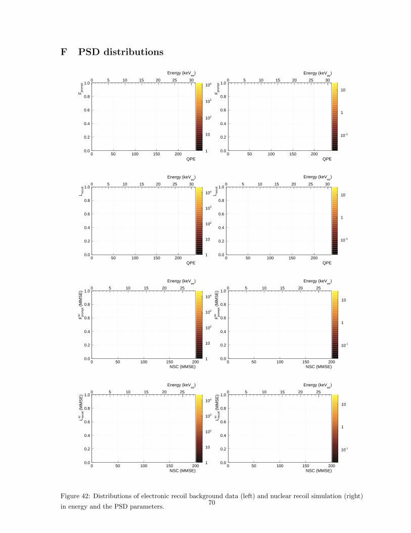
F PSD distributions
QPE0 50 100 150 200
prom
ptF
0.0
0.2
0.4
0.6
0.8
1.0
1
10
210
310
410
)ee
Energy (keV
0 5 10 15 20 25 30
QPE0 50 100 150 200
prom
ptF
0.0
0.2
0.4
0.6
0.8
1.0
1−10
1
10
)ee
Energy (keV
0 5 10 15 20 25 30
QPE0 50 100 150 200
reco
ilL
0.0
0.2
0.4
0.6
0.8
1.0
1
10
210
310
410
)ee
Energy (keV
0 5 10 15 20 25 30
QPE0 50 100 150 200
reco
ilL
0.0
0.2
0.4
0.6
0.8
1.0
1−10
1
10
)ee
Energy (keV
0 5 10 15 20 25 30
NSC (MMSE)0 50 100 150 200
(M
MS
E)
prom
ptsc
F
0.0
0.2
0.4
0.6
0.8
1.0
1
10
210
310
410
)ee
Energy (keV
0 5 10 15 20 25
NSC (MMSE)0 50 100 150 200
(M
MS
E)
prom
ptsc
F
0.0
0.2
0.4
0.6
0.8
1.0
1−10
1
10
)ee
Energy (keV
0 5 10 15 20 25
NSC (MMSE)0 50 100 150 200
(M
MS
E)
reco
ilsc L
0.0
0.2
0.4
0.6
0.8
1.0
1
10
210
310
410
)ee
Energy (keV
0 5 10 15 20 25
NSC (MMSE)0 50 100 150 200
(M
MS
E)
reco
ilsc L
0.0
0.2
0.4
0.6
0.8
1.0
1−10
1
10
)ee
Energy (keV
0 5 10 15 20 25
Figure 42: Distributions of electronic recoil background data (left) and nuclear recoil simulation (right)
in energy and the PSD parameters.70

/ ndf 2χ 68.54 / 67Prob 0.4249
µ 0.0003± 0.2558 b 0.00041± 0.02479
σ 0.00073± 0.03108 Z 28.2± 1370
promptF0.0 0.1 0.2 0.3 0.4 0.5 0.6 0.7 0.8 0.9 1.0
Cou
nts
1
10
210
310
410
510 / ndf 2χ 68.54 / 67
Prob 0.4249 µ 0.0003± 0.2558
b 0.00041± 0.02479 σ 0.00073± 0.03108
Z 28.2± 1370
100%
t.e.
promptF0.35 0.40 0.45 0.50 0.55 0.60 0.65
leak
P
10−10
9−10
8−10
7−10
6−10
5−10
4−10
3−10
2−10
1−10
50%
n.r
.a.
90%
n.r
.a.
Model
Data
/ ndf 2χ 35.87 / 53Prob 0.9656
µ 0.0001± 0.3324 b 0.00018± 0.01197
σ 0.0008± 0.0183 Z 92.4± 2299
recoilL0.0 0.1 0.2 0.3 0.4 0.5 0.6 0.7 0.8 0.9 1.0
Cou
nts
1
10
210
310
410
510
/ ndf 2χ 35.87 / 53Prob 0.9656
µ 0.0001± 0.3324 b 0.00018± 0.01197
σ 0.0008± 0.0183 Z 92.4± 2299
100%
t.e.
recoilL0.40 0.45 0.50 0.55 0.60 0.65
leak
P
10−10
9−10
8−10
7−10
6−10
5−10
4−10
3−10
2−10
1−10
50%
n.r.
a.
90%
n.r.
a.
Model
Data
/ ndf 2χ 67.68 / 67Prob 0.4537
µ 0.0001± 0.2853 b 0.00021± 0.02516
σ 0.00047± 0.02627 Z 29.1± 1695
(MMSE)promptscF
0.0 0.2 0.4 0.6 0.8 1.0
Cou
nts
1
10
210
310
410
510 / ndf 2χ 67.68 / 67
Prob 0.4537 µ 0.0001± 0.2853
b 0.00021± 0.02516 σ 0.00047± 0.02627
Z 29.1± 1695
100%
t.e.
(MMSE)promptscF
0.45 0.50 0.55 0.60 0.65 0.70
leak
P
10−10
9−10
8−10
7−10
6−10
5−10
4−10
3−10
2−10
1−10
50%
n.r
.a.
90%
n.r
.a.
Model
Data
/ ndf 2χ 58.37 / 57Prob 0.4249
µ 0.0001± 0.3206 b 0.0002± 0.0157
σ 0.00063± 0.01931 Z 72.6± 2305
(MMSE)recoilscL
0.0 0.1 0.2 0.3 0.4 0.5 0.6 0.7 0.8 0.9 1.0
Cou
nts
1
10
210
310
410
510 / ndf 2χ 58.37 / 57
Prob 0.4249 µ 0.0001± 0.3206
b 0.0002± 0.0157 σ 0.00063± 0.01931
Z 72.6± 2305
100%
t.e.
(MMSE)recoilscL
0.40 0.45 0.50 0.55 0.60 0.65 0.70
leak
P
10−10
9−10
8−10
7−10
6−10
5−10
4−10
3−10
2−10
1−10
50%
n.r
.a.
90%
n.r
.a.
Model
Data
Figure 43: Left: projections of the PSD-distributions between 110 and 120 QPE or 100 and 109 NSC
(approx. 15 keVee) are shown. Right: The leakage probability at the same energy as estimated from
data and the model.71
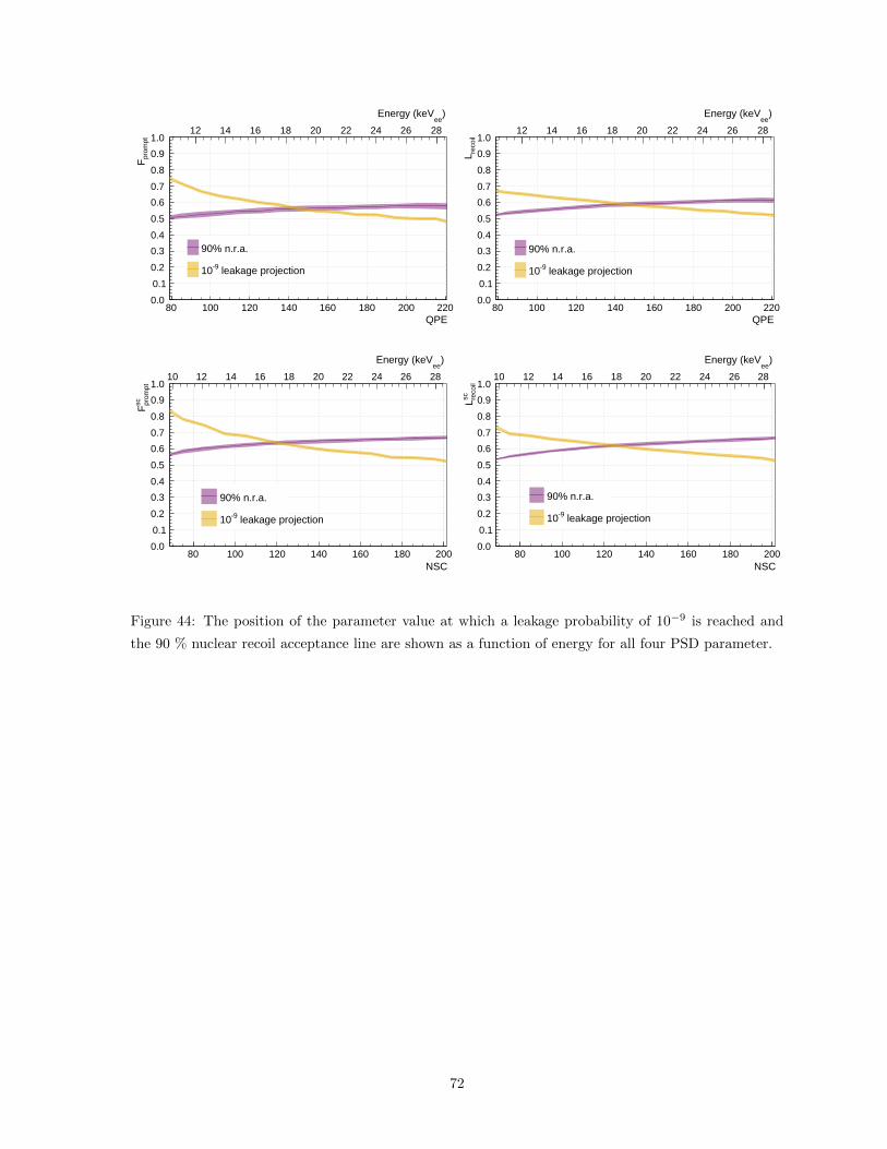
QPE80 100 120 140 160 180 200 220
prom
ptF
0.0
0.1
0.2
0.3
0.4
0.5
0.6
0.7
0.8
0.9
1.0
90% n.r.a.
leakage projection-910
)ee
Energy (keV
12 14 16 18 20 22 24 26 28
QPE80 100 120 140 160 180 200 220
reco
ilL
0.0
0.1
0.2
0.3
0.4
0.5
0.6
0.7
0.8
0.9
1.0
90% n.r.a.
leakage projection-910
)ee
Energy (keV
12 14 16 18 20 22 24 26 28
NSC80 100 120 140 160 180 200
prom
ptsc
F
0.0
0.1
0.2
0.3
0.4
0.5
0.6
0.7
0.8
0.9
1.0
90% n.r.a.
leakage projection-910
)ee
Energy (keV
10 12 14 16 18 20 22 24 26 28
NSC80 100 120 140 160 180 200
reco
ilsc L
0.0
0.1
0.2
0.3
0.4
0.5
0.6
0.7
0.8
0.9
1.0
90% n.r.a.
leakage projection-910
)ee
Energy (keV
10 12 14 16 18 20 22 24 26 28
Figure 44: The position of the parameter value at which a leakage probability of 10−9 is reached and
the 90 % nuclear recoil acceptance line are shown as a function of energy for all four PSD parameter.
72

References
[1] P.F. Smith. Dark matter detection. Physics Reports, 1990.
[2] D. Clowe. A direct empirical proof of the exsitence of dark matter. The Astrophysical Journal,
2006.
[3] Planck Collaboration. Planck 2015 results. i. overview of products and scientific results. Astronomy
and Astrophysics, 2015.
[4] K. Freese. Limits on stellar objects as the dark matter of our halo: Nonbaryonic dark matter seems
to be required. arXiv:astro-ph/9904401, 1999.
[5] Richard J. Gaitskell. Direct detection of dark matter. Annual Review of Nuclear and Particle
Science, 54(1):315–359, Dec 2004.
[6] M. Aaboud, G. Aad, B. Abbott, J. Abdallah, O. Abdinov, B. Abeloos, S. H. Abidi, O. S. AbouZeid,
N. L. Abraham, and et al. Search for dark matter at√s = 13 tev in final states containing an
energetic photon and large missing transverse momentum with the atlas detector. The European
Physical Journal C, 77(6), Jun 2017.
[7] IceCube Collaboration. Search for annihilating dark matter in the sun with 3 years of icecube data.
European Physical Journal, 2017.
[8] D. Hooper. Dark matter annihilation in the galactic center as seen by the fermi gamma ray space
telescope. Physics Letters B, 2011.
[9] Kluck. Search for low-mass dark matter with the cresst experiment. arXiv:1711.01285 [astro-ph.IM],
2017.
[10] C. Amole. Dark matter search results from the pico-60 c3f8 bubble chamber. Physical Review
Letters, 2017.
[11] DarkSide Collaboration. Darkside-50 532-day dark matter search with low-radioactivity argon.
arXiv:1802.07198, 2018.
[12] P.-A. Amaudruz. Measurement of the scintillation time spectra and pulse-shape discrimination of
low-energy beta and nuclear recoils in liquid argon with deap-1.pdf. Astroparticle Physics, 2016.
[13] C. E. Aalseth. Darkside-20k: A 20 tonne two-phase lar tpc for direct dark matter detection at lngs.
arXiv:1707.08145 [physics.ins-det], 2017.
[14] R. W. Schnee. Introduction to dark matter experiments. 2011.
[15] P. Benetti. Measurement of the specific activity of 39ar in natural argon. Nucl. Instrum. Methods
A, 2008.
[16] Sonnenschein. Measurement of ar39 in argon.
73
[17] T. Pollmann. Pulse shape discrimination studies in a liquid argon scintillation detector. Master’s
thesis, Max-Planck-Institut fuer Kernphysik, 2007.
[18] Akira Hitachi. Effect of ionization density on time dependence of luminescence from liquid argon
and xenon. Physical Review B, 1983.
[19] C. Amsler. Luminescence quenching of the triplet excimer state by air traces in gaseous argon.
JINST 3 P02001, 2008.
[20] M Miyajima, T Takahashi, S Konno, T Hamada, S Kubota, H Shibamura, and T Doke. Average
energy expended per ion pair in liquid argon. Phys. Rev. A, 9(3):1438–1443, 1974.
[21] A. Hitachi. Luminescence quenching in liquid argon under charged-particle impact: Relative scin-
tillation yield at different linear energy transfers. Physical Review B, 1992.
[22] C. Regenfus. Study of nuclear recoils in liquid argon with monoenergetic neutrons. Journal of
Physics: Conference Series 375, 2012.
[23] H. Cao. Measurement of scintillation and ionization yield and scintillation pulse shape from nuclear
recoils in liquid argon. Physical Review D, 2015.
[24] W. H. Lippincott, K. J. Coakley, D. Gastler, A. Hime, E. Kearns, D. N. McKinsey, J. A. Nikkel,
and L. C. Stonehill. Scintillation time dependence and pulse shape discrimination in liquid argon.
Physical Review C, 78(3), Sep 2008.
[25] T. Heindl. The scintillation of liquid argon. A Letters Journal Exploring the Frontiers of Physics,
2010.
[26] T. Doke. Absolute scintillation yields in liquid argon and xenon for various particles. Jpn. J. Appl.
Phys., 2002.
[27] R. Acciarri. Effects of nitrogen contamination in liquid argon. JINST, 2010.
[28] B.J.P. Jones. A measurement of the absorption of liquid argon scintillation light by dissolved
nitrogen at the part-per-million level. JINST, 2013.
[29] R Acciarri, M Antonello, B Baibussinov, M Baldo-Ceolin, P Benetti, F Calaprice, E Calligarich,
M Cambiaghi, N Canci, F Carbonara, and et al. Oxygen contamination in liquid argon: com-
bined effects on ionization electron charge and scintillation light. Journal of Instrumentation,
5(05):P05003–P05003, May 2010.
[30] DEAP Collaboration. The deap-3600 dark matter search experiment. Astroparticle Physics, 2017.
[31] Franksweb. http://www.frankswebspace.org.uk/scienceandmaths/physics/physicsgce/d1-5.htm.
[32] The DEAP Collaboration. In-situ characterization methods for the hamamatsu 5912 photomultiplier
tubes used in the deap-3600 experiment. JINST, 2017.
[33] H.O. Meyer. Dark rate of a photomultiplier at cryogenic temperatures.
74
[34] K. J. Ma. Time and amplitude of afterpulse measured with a large size photomultiplier tube.
Nuclear Instruments and Methods A, 2009.
[35] J.E.McMillan. Neutron shielding for particle astrophysics experiments. arXiv:physics/0510186,
2008.
[36] D. Mei. Evaluation of (α, n) induced neutrons as a background for dark matter experiments.
Astroparticle Physics, 2009.
[37] Provided by Bjoern Lehnert, DEAP Collaboration.
[38] E. Segreto. Evidence of delayed light emission of tetraphenyl-butadiene excited by liquid-argon
scintillation light. Physical Review C, 91(3), Mar 2015.
[39] C. J. Stanford. Alphas and surface backgrounds in liquid argon dark matter detectors. Master’s
thesis, Princeton University, 2017.
[40] R.J. Holmes. Use of Nuclear Techniques Use of Nuclear Techniques in the Mineral Industry. Aus-
tralian Atomic Energy Commission Reseach Establishment Lucas Heights, 1982.
[41] Provided by Jocelyn Monroe, DEAP Collaboration.
[42] Bryce Marchick. Internal analysis. University of Alberta.
[43] DEAP Collaboration. First results from the deap-3600 dark matter search with argon at snolab.
arXiv:1707.08042v2, 2017.
[44] DEAP Collaboration. Measurement of the scintillation time spectra and pulse-shape discrimination
of low-energy betas and nuclear recoils in liquid argon with deap-1. Astroparticle Phyiscs, 2016.
[45] E. Gatti. A new linear method of discrimination between elemantary particles in scintillation
counters.
[46] J. Neyman. On the problem of the most efficient tests of statistical hypotheses. Philosophical
Transactions of the Royal Society A: Mathematical, Physical and Engineering Sciences., 1933.
[47] M. Akashi-Ronquest. Improving photoelectron counting and particle identification in scintillation
detectors with bayesian techniques. Astroparticle Physics, 2014.
[48] Provided by Joseph Walding, DEAP Collaboration.
[49] E. Wilson. Probable inference, the law of succession, and statistical inference. Journal of the
American Statistical Association, 22(158), 1927.
[50] P.-A. Soderstrom. Digital pulse-shape discrimination of fast neutrons and γ rays. arXiv:0805.0692v1,
2008.
[51] T. Bayes. An essay towards solving a problem in the doctrine of chances. by the late rev. mr. bayes,
communicated by mr. price, in a letter to john canton, m. a. and f. r. s. 1763.
[52] Provided by Alistair Butcher, DEAP Collaboration.
75

[53] G. Verghese A. Oppenheim. Signals, Systems and Inference, volume 1 edition. Pearson, 2015.
[54] Jan-Henrik Schmidt-Dencker. Stability of the prompt fraction discriminator in the deap-3600 dark
matter experiment. Master’s thesis, TU Munchen, 2018.
76

Glossary
PMT trace , or event trace: PMT signal as a function of time in a single event
Pulse shape , or average pulse shape: sum of PMT traces over many events across the PMT array
keVee unit for the detector signal intensity in terms of the energy in keV of an electronic recoil which
would cause the same intensity
Q Integrated charge normalized by the PMT’s single-photoelectron charge
nnsc Estimate for the number of photons and dark hits in a pulse based on a Bayesian analysis. Unless
otherwise specified, the MMSE (Minimum mean square error) estimator is used
Fprompt Prompt-window-based discriminator using normalized charge (QPE) with a 88 ns prompt
window and 10 µs late window
Lrecoil Likelihood-based discriminator using normalized charge (QPE) as defined in equation 26. Un-
less otherwise specified, photon weights based on model PDFs as shown in figure 20are used.
F scprompt Prompt-window-based discriminator using nnsc with a 88 ns prompt window and 10 µs late
window. Unless otherwise specified, the MMSE estimate is used.
Lscrecoil Likelihood-based discriminator using nnsc. Unless otherwise specified, photon weights based on
model PDFs as shown in figure 20 and the MMSE estimate are used.
77

Acknowledgements
I have gotten very lucky to find a supervisor in Tina who is not only very knowledgeable about physics
and computers, but also took the time to share her wisdom. I could not have asked for better support.
Also, thank you for integrating me very well into the rest of the collaboration on the other side of the
Atlantic, which gave me the chance to meet and work with many other great scientists. I congratulate
the members of the DEAP collaboration for building a fantastic detector.
I also would like to thank Prof. Schonert for entrusting me with this topic and his generosity in allowing
me to visit two collaboration meetings. I also thank my ’roommates’ in the student’s office for being
very fun companions over the past twelve months.
78