Background Aerosol in the United States:Natural Sources and Transboundary Pollution

Naresh Kumar, Ph.D.

EPRI, Palo Alto, CA

Presented at

MANE-VU/MARAMA 2004 Science Meeting January 28, 2004

Baltimore, MD

2

Outline

• “Natural Visibility” as defined by EPA for implementation of Regional Haze Rule

• Study by Dr. Daniel Jacob and his group at Harvard

• Results from the above study– Taken from presentation given by Dr. Jacob at the RPO

meeting in November 2003

• Future work

3

Issues with EPA’s Definition of “Natural Visibility” Conditions

• Based on Trijonis (1990)– Trijonis used best information available at that time and

provided uncertainty bounds of 2-3 on his estimates

– Lot more information available since then

– Incumbent upon scientific community to use new information along with more analysis to come up with better estimates of natural levels

• Should transboundary pollution be included in definition of 2064 endpoint?– U.S. has no control over overseas emissions

– Transboundary impact likely to go up

– This issue will become even more important in second and successive implementation periods

4

Issues with EPA’s Definition of “Natural Visibility” Conditions (Contd.)

• OCM/OC ratio– Currently, IMPROVE uses a factor of 1.4 to go from Organic

Carbon measurements to Organic Carbon Mass

– Turpin and Lim (2001) suggest a factor of 2.1 for aged aerosols

– This will have significant effect for the 2064 endpoint as OC is the largest component

• IMPROVE equation ignores sea-salt– Important for coastal sites

– Sea-salt starts absorbing water at lower RH than does ammonium sulfate, but both behave similarly between RH of 60-90 percent

5

Issues with EPA’s Definition of “Natural Visibility” Conditions (Contd.)

• Fire and dust events– These events occur mostly in spring and summer, so their

impact on “natural levels” of soil, EC and OC during those periods may be disproportionately higher

– The natural value of 0.5 g/m3 proposed by Trijonis should account for some of the impact from wildfires on annual basis, but need to determine impact by season

6

Issues with EPA’s Definition of “Natural Visibility” Conditions (Contd.)

• Current approach for estimating natural visibility for 20% worst days– 20% Worst (dv) = Annual Average (dv) + 1.28 σ

– σ = 2 dv (sites in West) and 3 dv (sites in East)

• Problems with this approach:

– 1.28 corresponds to 90th percentile for a “normal” distribution, but average of 20% worst days occurs at 92nd percentile giving a factor of 1.4

– Work done by Sonoma Technology, Inc. (STI), using actual data scaled to “natural levels”, suggests using a factor of 1.5 and σ of 3.0 for West and 3.5 for East

7

Effect of STI’s Approach on 20% Worst Natural Conditions

 

 

Class I Site EPA Default Approach (dv)

STI Approach (dv)

Increase (dv)

Acadia 11.48 13.09 1.61

Big Bend 6.99 8.84 1.85

Boundary Waters 11.21 12.36 1.15

Grand Canyon 6.97 8.81 1.84

Great Smoky 11.51 12.72 1.21

Mount Rainier 7.85 9.87 2.02

The natural condition values (for 20% worst days) estimated by the STI approach are 1.2 to 2.0 dv greater than those determined by EPA’s default method

8

Work done by Dr. Jacob and Co-workers

• Use of a global chemistry model to estimate natural and background levels of aerosols to answer the following questions:

– How good are the “default estimated natural PM concentrations” proposed by EPA as 2064 endpoint for application of the Regional Haze Rule?

– To what extent does transboundary pollution compromise achievability of natural PM concentrations?

9

2004-2018 Emission Reductions for the RHRare Strongly Sensitive to Choice of 2064 Endpoint

Conceptual calculation for mean western U.S. conditions, assuming linear relationship between emissions and bext

Desired trend in visibility

Required % decrease of U.S. anthropogenic emissions

Phase 1

30%

48%

, ,10ln10

ext natural ext anthropb bdv

10

Strategy for Quantifying Background PM Concentrations in United States

Quantify natural aerosol

concentrations

Quantify transboundary

pollution

Start from best a priori estimates of natural and anthropogenic PM

sources

Simulate PM concentrations with GEOS-CHEM global model

Evaluate with observations from IMPROVE, CASTNET, other networks

Improvedemissionestimates

Conduct sensitivity simulations

11

GEOS-CHEM Global Chemical Transport Model(http://www-as.harvard.edu/chemistry/trop/geos)

• Driven by NASA/GEOS-3 assimilated meteorological data with 2ox2.5o horizontal resolution, 48 levels in vertical

• Carbonaceous aerosol simulation (OC, EC) for 1998Park, R.J., D.J. Jacob, M. Chin, and R.V. Martin, Sources of carbonaceous aerosols over the

United States: implications for natural visibility, J. Geophys. Res.., 108, 4355, 2003.

• Coupled oxidant –sulfate-nitrate-ammonium simulation for 2001 (also 1998)Park, R.J., D.J. Jacob, et al., Natural and transboundary influences on ammonium-sulfate-nitrate

aerosols in the United States: implications for visibility, J. Geophys. Res., manuscript submitted

12

Carbonaceous Aerosol SimulationBest a priori sources (1998)

ORGANIC CARBON (OC) ELEMENTAL CARBON (EC)

GLOBAL

UNITEDSTATES

130 Tg yr-1 22 Tg yr-1

2.7 Tg yr-1 0.66 Tg yr-1

13

Biomass Burning Emissions In GEOS-CHEM:Climatology from Duncan, Logan, et al. [JGR 2002] scaled to 1998using TOMS and ATSR satellite data

Inter-annual variability derived from TOMS Aerosol Index [Duncan et al., 2002] 1998 fires from ATSR satellite data:

• Apr-May fires in Mexico•Jul-Sep fires in U.S/Canada

14

Seasonal Variation of OC and ECConstrain OC/EC sources using simulation of monthly mean IMPROVE observations and model tracers of individual source types.

IMPROVE

modelmodel tracers(additive)

biomass burningvegetationfossil fuelbiofuel

15

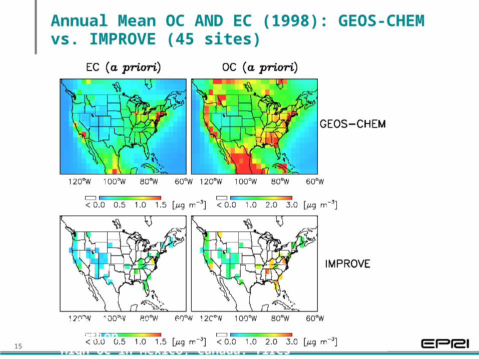
Annual Mean OC AND EC (1998): GEOS-CHEM vs. IMPROVE (45 sites)

• High OC in southeast U.S.: vegetation• High OC in Mexico, Canada: fires

16

Least-squares Fit of Model to Observations Generates Optimized a Posteriori Sources

Fossil fuel 15% Biofuel 65% Biomass burning 17% Biogenic 11%

17

Carbonaceous Aerosol in the U.S.:Contributions from Natural Sources and Transboundary Pollution

Annual regional means from GEOS-CHEM standard and sensitivity simulations

OC (g m-3 as OMC)

West East

EC (g m-3)

West East

Baseline (1998) 2.0 3.2 0.30 0.68

Zero anthropogenic emissions in U.S.

– GEOS-CHEM (w/ climatological fires)

– EPA default values1.3

0.5

1.2

1.4

0.06

0.02

0.04

0.02

Contributions from transboundary anthropogenic sources

Canada and Mexico

Asia0.05

0.013

0.05

0.007

0.02

0.005

0.02

0.003

•We find that EPA default natural concentrations are too low by factors of 2-3 except for OC in eastern U.S. – quantifying fire influences is critical

•Transboundary pollution influences are relatively small except for EC from Canada/Mexico

18

H2SO4-HNO3-NH3-H2O Aerosol simulationGEOS-CHEM emissions (2001)

GLOBAL UNITED STATES

Sulfur,Tg S yr-1

Ammonia,Tg N yr-1

NOx,Tg N yr-1

78 8.3

55 2.8

43 7.4

19

Annual Mean Sulfate (2001): GEOS-CHEM vs. IMPROVE (141 sites)

20

Sulfate at IMPROVE, CASTNET, NADP (deposition) Sites:model vs. observed for different seasons

High correlation, no significant model bias except NADP summer

21

Annual Mean Ammonium (2001): GEOS-CHEM vs. CASTNET (79 sites)

(no ammonium data at IMPROVE sites)

22

Annual Mean Nitrate (2001): GEOS-CHEM vs. CASTNET (79 sites)

23

Ammonium and Nitrate at CASTNET and IMPROVE Sites:model vs. observed for different seasons

Ammonium Nitrate Nitrate

• High bias for NH4+ in fall:

error in seasonal variation of livestock emissions

• High bias for NO3-, esp. in

summer/fall, results from bias on [SO4

2-]-2[NH4+]

24

Sulfate-Nitrate-Ammonium Aerosol in the U.S.: Contributions from Natural Sources and Transboundary Pollution

Annual regional means from GEOS-CHEM standard and sensitivity simulations

Ammonium sulfate (g m-3)

West East

Ammonium Nitrate (g m-3)

West East

Baseline (2001) 1.52 4.11 1.53 3.26

Zero anthropogenic emissions in U.S.

– GEOS-CHEM

– EPA default values0.43

0.11

0.38

0.23

0.27

0.1

0.37

0.1

Contributions from transboundary anthropogenic sources

Canada and Mexico

Asia0.15

0.13

0.14

0.12

0.20

-0.02

0.25

-0.02

•Achievability of EPA default estimates is compromised by transboundary pollution influences

•Transboundary pollution influence from Asia is comparable in magnitude to that from Canada + Mexico

25

Background and natural levels using the GEOS-CHEM model compared to EPA’s default estimates of natural levels

 

Class I site

Ammonium Sulfate (g/m3) Organic Carbon Mass (g/m3)

EPA Default

 Natural level using

GEOS-CHEM

Background level using

GEOS-CHEM

EPA Default

Natural level using

GEOS-CHEM

Background level using

GEOS-CHEM

Acadia 0.23 0.13 0.39 1.4 0.95 1.01

Big Bend 0.11 0.13 0.54 0.47 1.44 1.50

Boundary Waters 0.23 0.11 0.51 1.4 1.26 1.32

Grand Canyon 0.11 0.12 0.49 0.47 0.87 0.93

Great Smoky 0.23 0.09 0.34 1.4 1.37 1.43

Mount Rainier 0.11 0.16 0.39 0.47 2.94 2.99

GEOS-CHEM OCM concentrations for sites in the West higher by a factor of 2 to 3 relative to the EPA default approach

The incorporation of transboundary emissions increases sulfate by 50% to 400% in class I areas relative to the EPA default approach

26

Model Evaluation with Asian Outflow Observations of Sulfate from Trace-p Aircraft Campaign (Mar-Apr 2001)

model

obs

110 E 120 E 130 E 140 E 150 E 160 E

Longitude

0 N

10 N

20 N

30 N

40 N

50 N

Lat

itu

de

DC-8 FlightsP-3B Flights

Observations from Jordan et al. [[JGR 2003]

27

Intercontinental Transport of Asian and North American Anthropogenic Sulfate

As determined from GEOS-CHEM 2001 sensitivity simulations with these sources shut off

Asiananthropogenicsulfate

N. Americananthropogenicsulfate

28

Future Work proposed by Dr. Jacob

• Correct known model flaws and increase model resolution – Overestimate of OC in the northwest

– Overestimate of ammonium in fall

– Increasing the resolution to 1ox1o should improve spatial resolution of coastal and topographical effects

• Provide model results in form most pertinent to the RHR – Calculation of natural and background levels for 20% worst

days

– Extract the baseline and natural PM concentrations at individual IMPROVE sites rather than just providing numbers for the east and the west

29

Future Work (Contd.)

• Improve confidence in baseline PM estimates and provide uncertainty ranges – Evaluation of soil simulation

– Better estimates of fire emissions

• Assess the impact of global changes in climate and emissions on baseline PM concentrations in the U.S. – Conduct 2050 simulation to examine (separately and in

concert) the effects of climate change and the effects of changes in emissions

– Estimate natural concentrations of PM at all IMPROVE sites for 2050 conditions

30

Final Thoughts

• RPOs, EPA, industry should leverage resources to better define the 2064 endpoint for RHR

• Global models are the best tools at present to synthesize all the data and provide estimates for that endpoint

• Data analysis and global modeling groups need to work together in this effort

• Global models can also provide boundary conditions to the regional models that would be used for developing implementation plans