backgammon articles · backgammon articles main page rules play sites software matches articles...
TRANSCRIPT
Backgammon Articles
Main Page Rules Play Sites Software Matches Articles
BACKGROUND LEARNING FACE-TO-FACE STRATEGY TECHNICAL COMPUTERS
R.G.B Archive Glossary Web Sites Motif Plays Backgammon Humor
Comments:[email protected]
Backgammon Articles
ProbabilityLuck versus Skill
Match PlayRatings
Probability
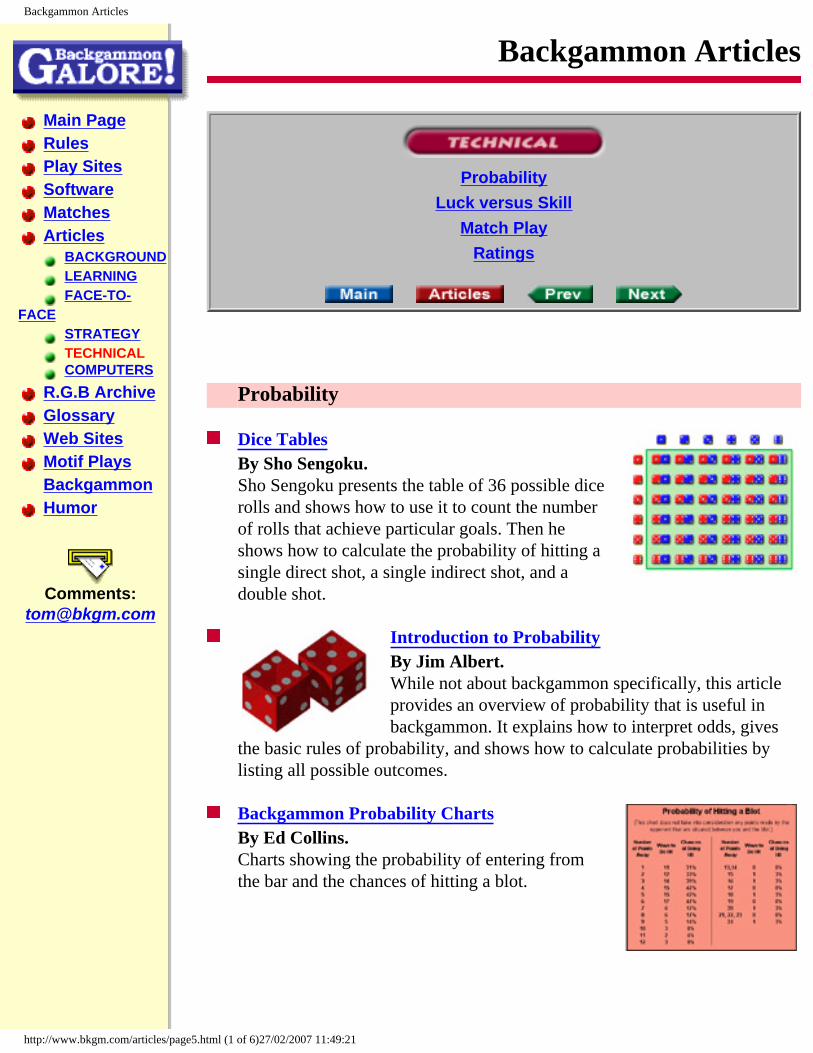
Dice Tables By Sho Sengoku. Sho Sengoku presents the table of 36 possible dice rolls and shows how to use it to count the number of rolls that achieve particular goals. Then he shows how to calculate the probability of hitting a single direct shot, a single indirect shot, and a double shot.
Introduction to Probability By Jim Albert. While not about backgammon specifically, this article provides an overview of probability that is useful in backgammon. It explains how to interpret odds, gives
the basic rules of probability, and shows how to calculate probabilities by listing all possible outcomes.
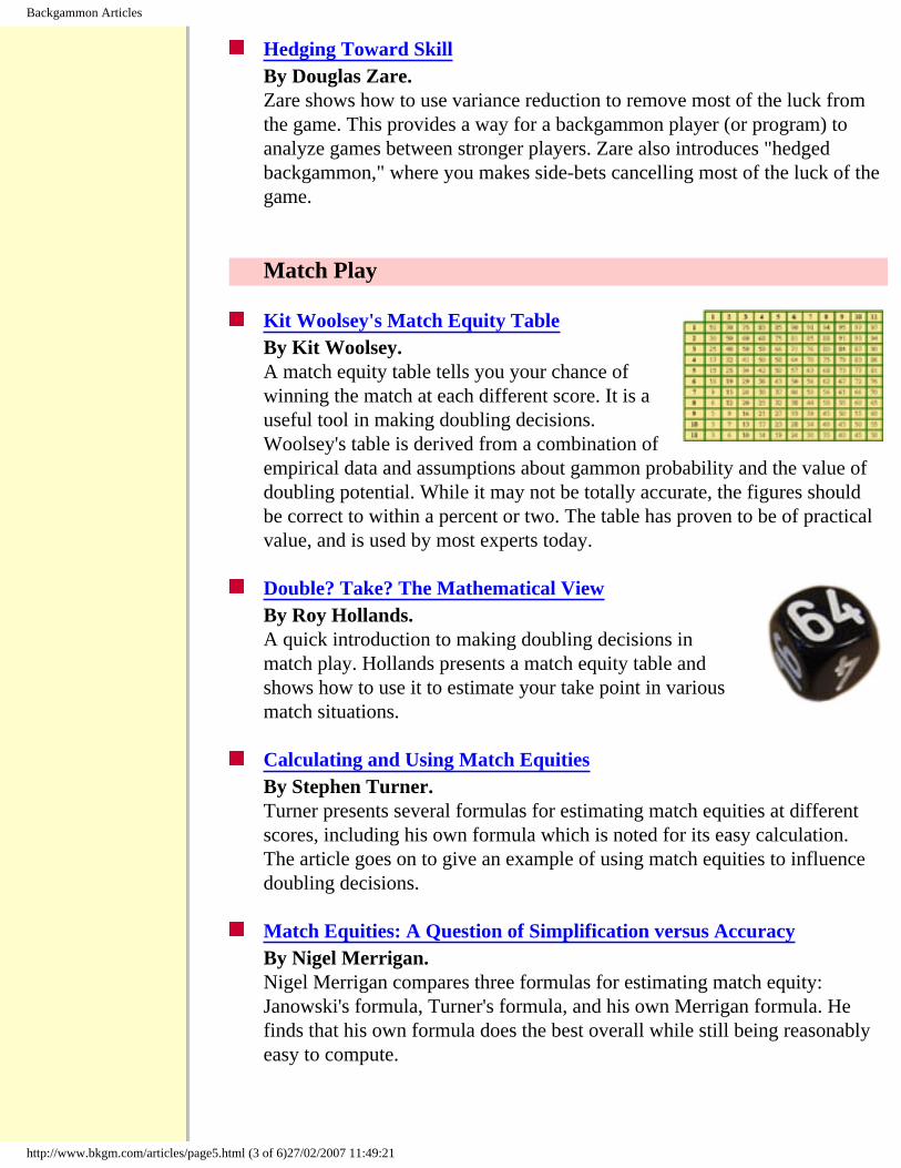
Backgammon Probability Charts By Ed Collins. Charts showing the probability of entering from the bar and the chances of hitting a blot.
http://www.bkgm.com/articles/page5.html (1 of 6)27/02/2007 11:49:21
Backgammon Articles
Dice Rolls and Probability in Backgammon By Paul Stephens. Understanding the true probabilities of dice rolls can greatly improve your tactical play, by letting you accurately assess the risk of leaving blots, and the chances of hitting and covering points.
Arithmetic techniques Sho Sengoku. Handy techniques for calculating terms that commonly come up in backgammon.
Probability and Statistics Posts Articles on probability and statistics in backgammon. Collected postings from the rec.games.backgammon newsgroup.
Luck versus Skill
A Backgammon Gamble Pays Off From the September 1982 issue of Games Magazine. Is backgammon a game of skill or chance? In 1982, a U.S. court answered that question in a decision that may affect backgammon players and promoters throughout the country.
A Measure of Luck By Douglas Zare. Can we measure luck in backgammon? What criteria should a measure of luck satisfy? Zare defines how to measure luck in backgammon and gives some interesting properties of luck.
Luck-versus-Skill Postings Articles about the role of luck and skill in backgammon. Collected postings from the rec.games.backgammon newsgroup.
http://www.bkgm.com/articles/page5.html (2 of 6)27/02/2007 11:49:21
Backgammon Articles
Hedging Toward Skill By Douglas Zare. Zare shows how to use variance reduction to remove most of the luck from the game. This provides a way for a backgammon player (or program) to analyze games between stronger players. Zare also introduces "hedged backgammon," where you makes side-bets cancelling most of the luck of the game.
Match Play
Kit Woolsey's Match Equity Table By Kit Woolsey. A match equity table tells you your chance of winning the match at each different score. It is a useful tool in making doubling decisions. Woolsey's table is derived from a combination of empirical data and assumptions about gammon probability and the value of doubling potential. While it may not be totally accurate, the figures should be correct to within a percent or two. The table has proven to be of practical value, and is used by most experts today.
Double? Take? The Mathematical View By Roy Hollands. A quick introduction to making doubling decisions in match play. Hollands presents a match equity table and shows how to use it to estimate your take point in various match situations.
Calculating and Using Match Equities By Stephen Turner. Turner presents several formulas for estimating match equities at different scores, including his own formula which is noted for its easy calculation. The article goes on to give an example of using match equities to influence doubling decisions.
Match Equities: A Question of Simplification versus Accuracy By Nigel Merrigan. Nigel Merrigan compares three formulas for estimating match equity: Janowski's formula, Turner's formula, and his own Merrigan formula. He finds that his own formula does the best overall while still being reasonably easy to compute.
http://www.bkgm.com/articles/page5.html (3 of 6)27/02/2007 11:49:21
Backgammon Articles
Graphical Match Equity Charts By Sho Sengoku. Using these charts, you can visualize important characteristics of the possible scores in a match.
How to Compute a Match Equity Table By Tom Keith. This article describes how a match equity table can be derived mathematically if you assume a constant gammon rate and efficient cube usage. Lots of diagrams show the process step by step.
Match Equities
Various match equity tables and formulas for estimating match equities collected from the rec.games.backgammon newsgroup.
Match Play Doubling Strategy By Tom Keith. In tournament play, where matches are played to a specified number of points, proper doubling strategy is different than when games are played for money. This article presents a number of the considerations a player must make when handling the cube in match play.
Abnormal Checker Plays in Matches By Wai Mun Yoon. One of the problems in match play is that correct checker play can depend on the match situation. An example is avoiding high volatility situations where a free-drop condition exists. Armed with the neural-net program Jellyfish and Woolsey's match equity table, Wai Mun Yoon sets out to discover some general rules to help the aspiring intermediate decide when to make a money-averse plays.
Match Play Articles about doubling strategy in match play. Collected postings from the rec.games.backgammon newsgroup.
http://www.bkgm.com/articles/page5.html (4 of 6)27/02/2007 11:49:21
Backgammon Articles
And the Trailer Doubles ... By Anthony Patz. Anthony Patz shows that when both players are two points away from winning the match, it can pay to double even when you are the underdog in the current game.
Match Play at 2-away/2-away Articles posted to the rec.games.backgammon newsgroup about the correct doubling strategy when both players both have two points to go in the match.
Ratings
The FIBS Rating System By Kevin Bastian. How do ratings on FIBS work? This article explains the rating formula and shows how the length of the match, each player's experience, and the difference in the players' ratings affect your rating when you win or lose a match. A similar ratings system is used on many other backgammon play sites.
The Rating System on the MicrosoftGaming Zone By Hank Youngerman. How do ratings work? What factors go into the ratings formula? What factors don't matter? What's the best way to increase my rating? Can ratings be manipulated?
Is the Elo Rating System a Good Fit to Backgammon Matches? By Gary Wong. The ratings formula on many backgammon servers is based on the work Arpad Elo did with chess ratings. How well does the Elo system work in backgammon? And how well does the FIBS implementation of Elo's formula work for describing the distribution of results for matches of different lengths?
http://www.bkgm.com/articles/page5.html (5 of 6)27/02/2007 11:49:21
Backgammon Articles
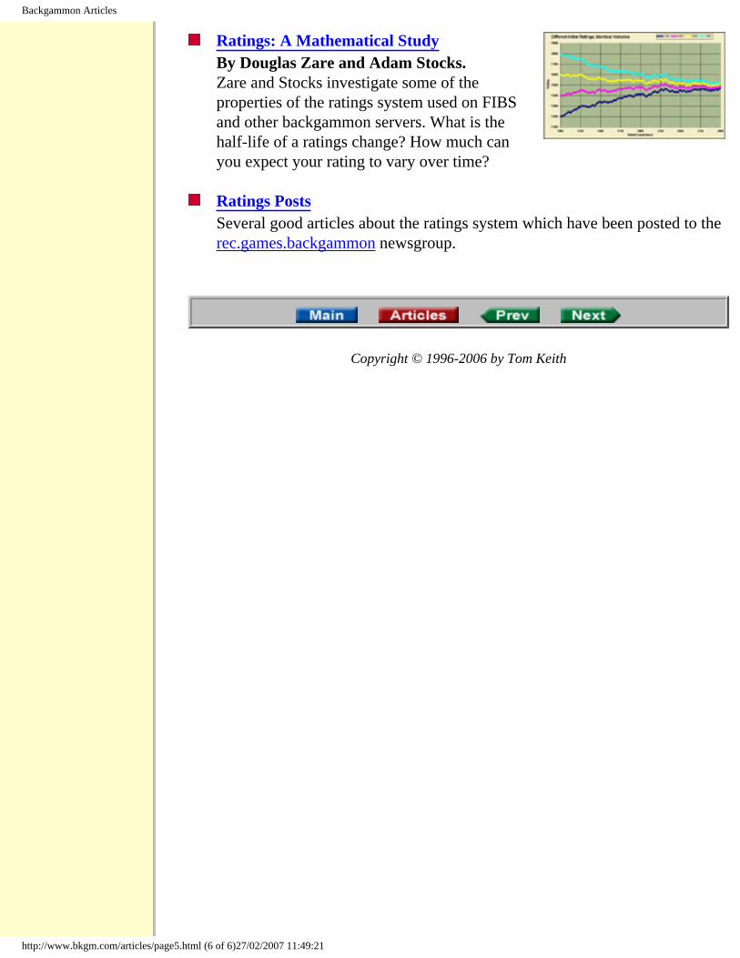
Ratings: A Mathematical Study By Douglas Zare and Adam Stocks. Zare and Stocks investigate some of the properties of the ratings system used on FIBS and other backgammon servers. What is the half-life of a ratings change? How much can you expect your rating to vary over time?
Ratings Posts Several good articles about the ratings system which have been posted to the rec.games.backgammon newsgroup.
Copyright © 1996-2006 by Tom Keith
http://www.bkgm.com/articles/page5.html (6 of 6)27/02/2007 11:49:21
Dice table
Dice tables
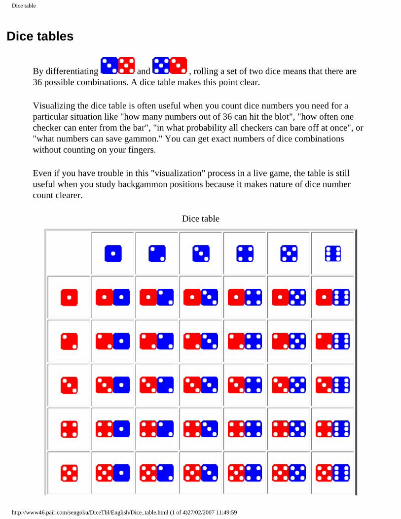
By differentiating and , rolling a set of two dice means that there are 36 possible combinations. A dice table makes this point clear.
Visualizing the dice table is often useful when you count dice numbers you need for a particular situation like "how many numbers out of 36 can hit the blot", "how often one checker can enter from the bar", "in what probability all checkers can bare off at once", or "what numbers can save gammon." You can get exact numbers of dice combinations without counting on your fingers.
Even if you have trouble in this "visualization" process in a live game, the table is still useful when you study backgammon positions because it makes nature of dice number count clearer.
Dice table
http://www46.pair.com/sengoku/DiceTbl/English/Dice_table.html (1 of 4)27/02/2007 11:49:59
Dice table
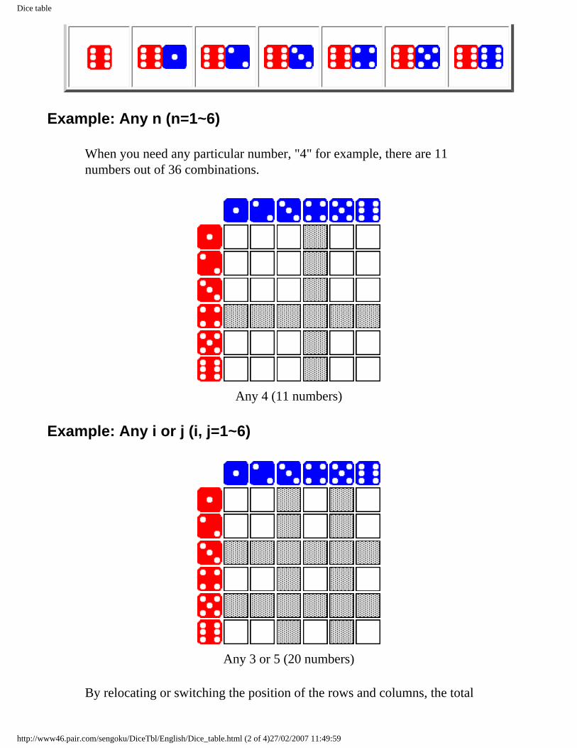
Example: Any n (n=1~6)
When you need any particular number, "4" for example, there are 11 numbers out of 36 combinations.
Any 4 (11 numbers)
Example: Any i or j (i, j=1~6)
Any 3 or 5 (20 numbers)
By relocating or switching the position of the rows and columns, the total
http://www46.pair.com/sengoku/DiceTbl/English/Dice_table.html (2 of 4)27/02/2007 11:49:59
Dice table
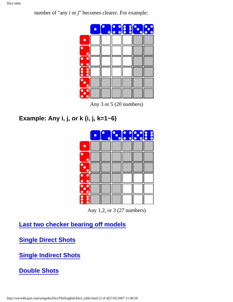
number of "any i or j" becomes clearer. For example:
Any 3 or 5 (20 numbers)
Example: Any i, j, or k (i, j, k=1~6)
Any 1,2, or 3 (27 numbers)
Last two checker bearing off models
Single Direct Shots
Single Indirect Shots
Double Shots
http://www46.pair.com/sengoku/DiceTbl/English/Dice_table.html (3 of 4)27/02/2007 11:49:59

Dice table
Created by Sho Sengoku
<<Prev Next>> Site top Dice table top
http://www46.pair.com/sengoku/DiceTbl/English/Dice_table.html (4 of 4)27/02/2007 11:49:59
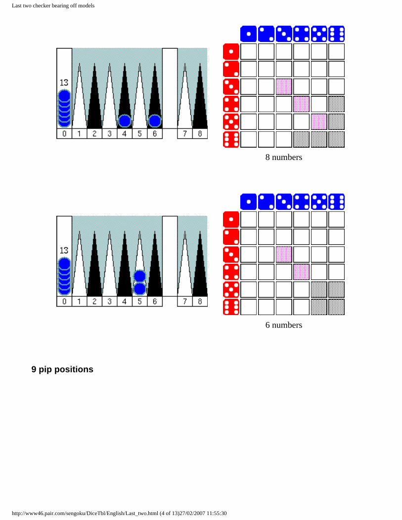
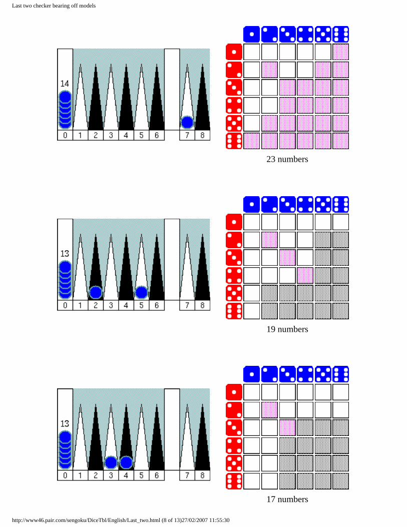
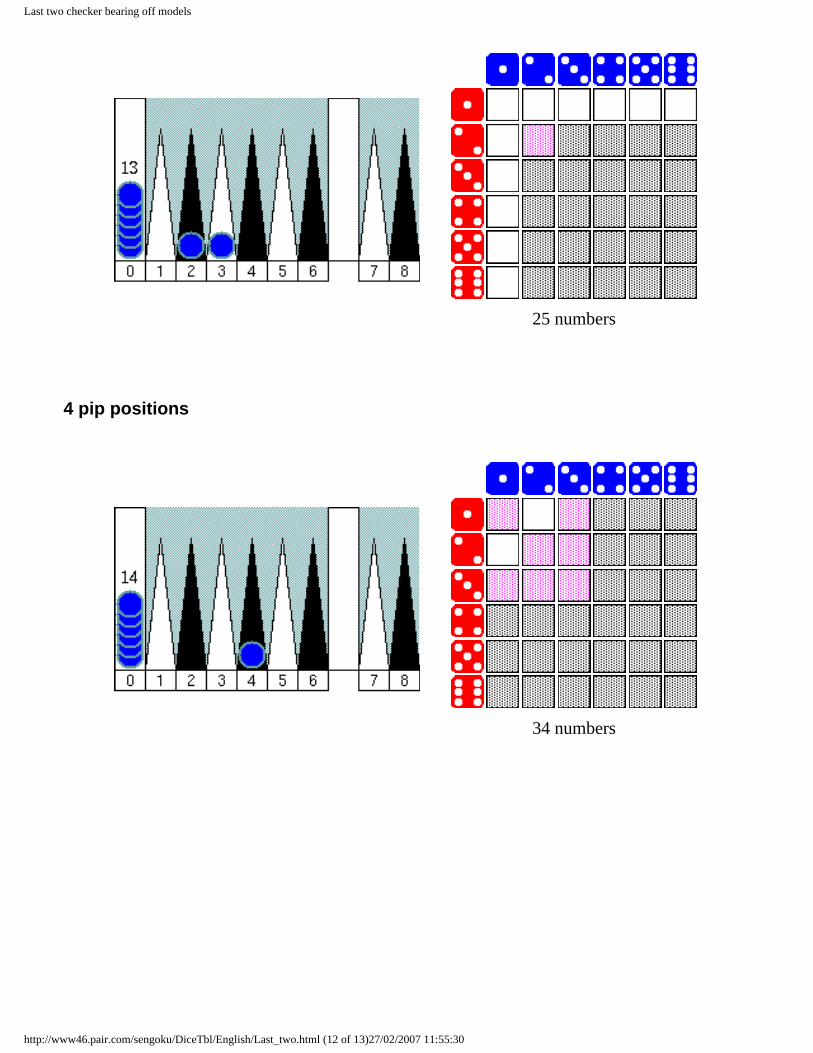
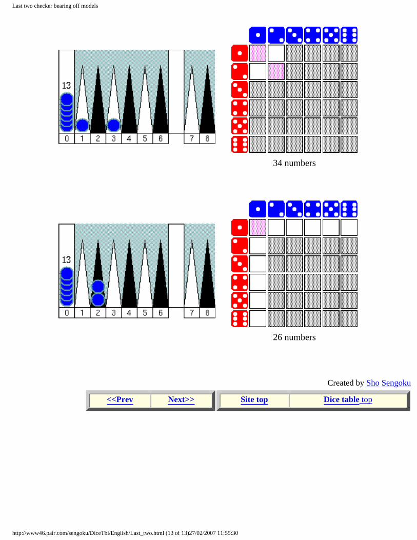
Last two checker bearing off models
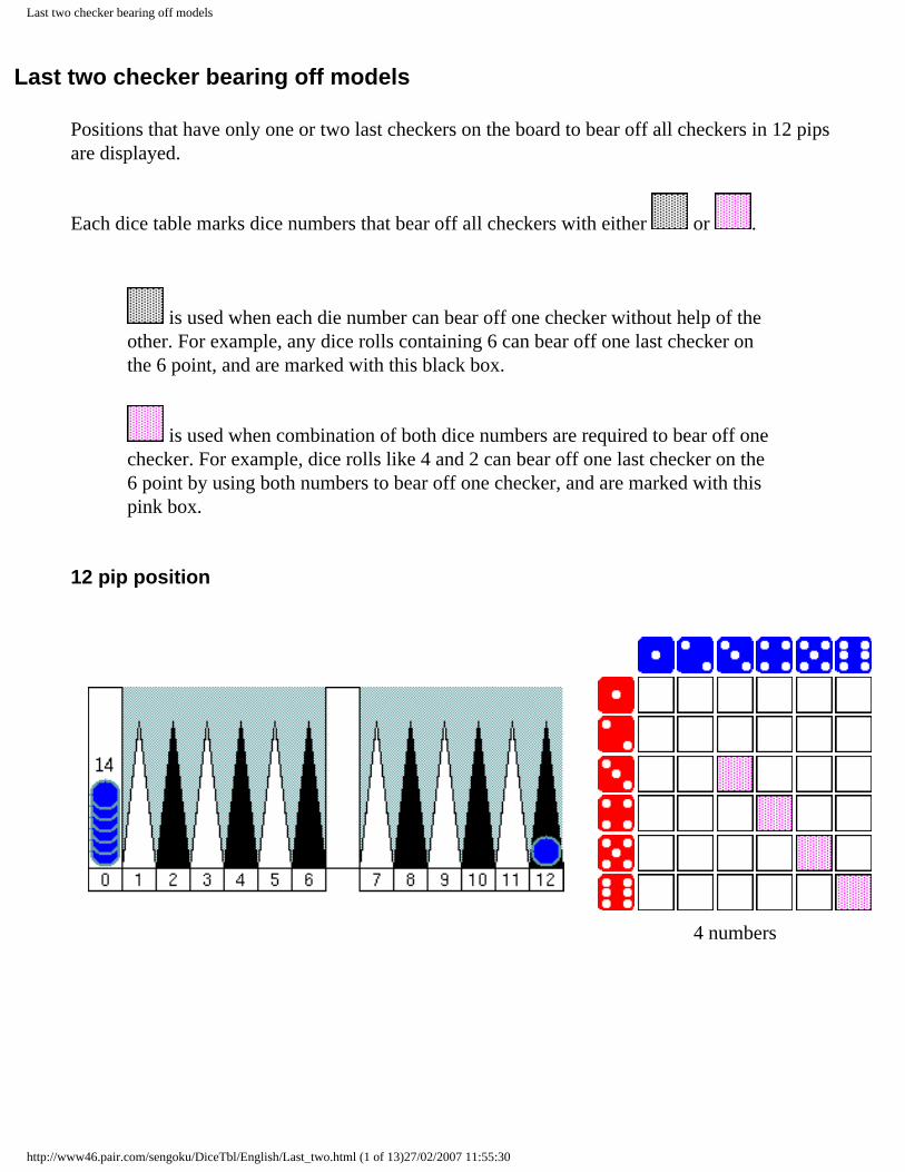
Last two checker bearing off models
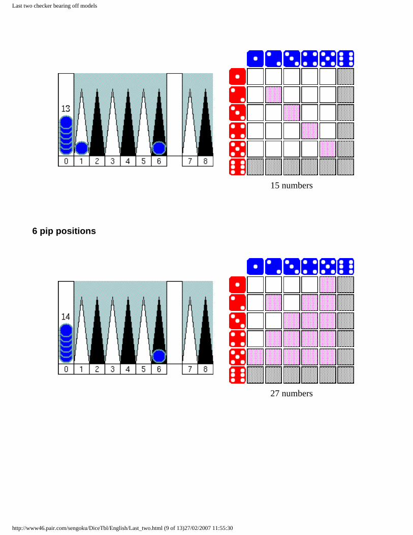
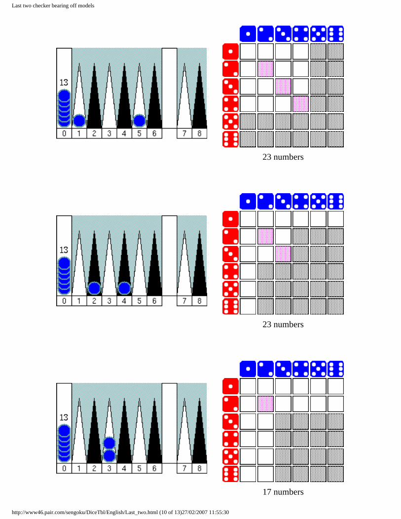
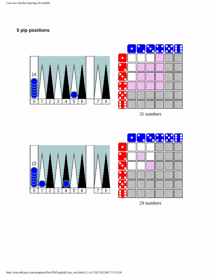
Positions that have only one or two last checkers on the board to bear off all checkers in 12 pips are displayed.
Each dice table marks dice numbers that bear off all checkers with either or .
is used when each die number can bear off one checker without help of the other. For example, any dice rolls containing 6 can bear off one last checker on the 6 point, and are marked with this black box.
is used when combination of both dice numbers are required to bear off one checker. For example, dice rolls like 4 and 2 can bear off one last checker on the 6 point by using both numbers to bear off one checker, and are marked with this pink box.
12 pip position
4 numbers
http://www46.pair.com/sengoku/DiceTbl/English/Last_two.html (1 of 13)27/02/2007 11:55:30
Last two checker bearing off models
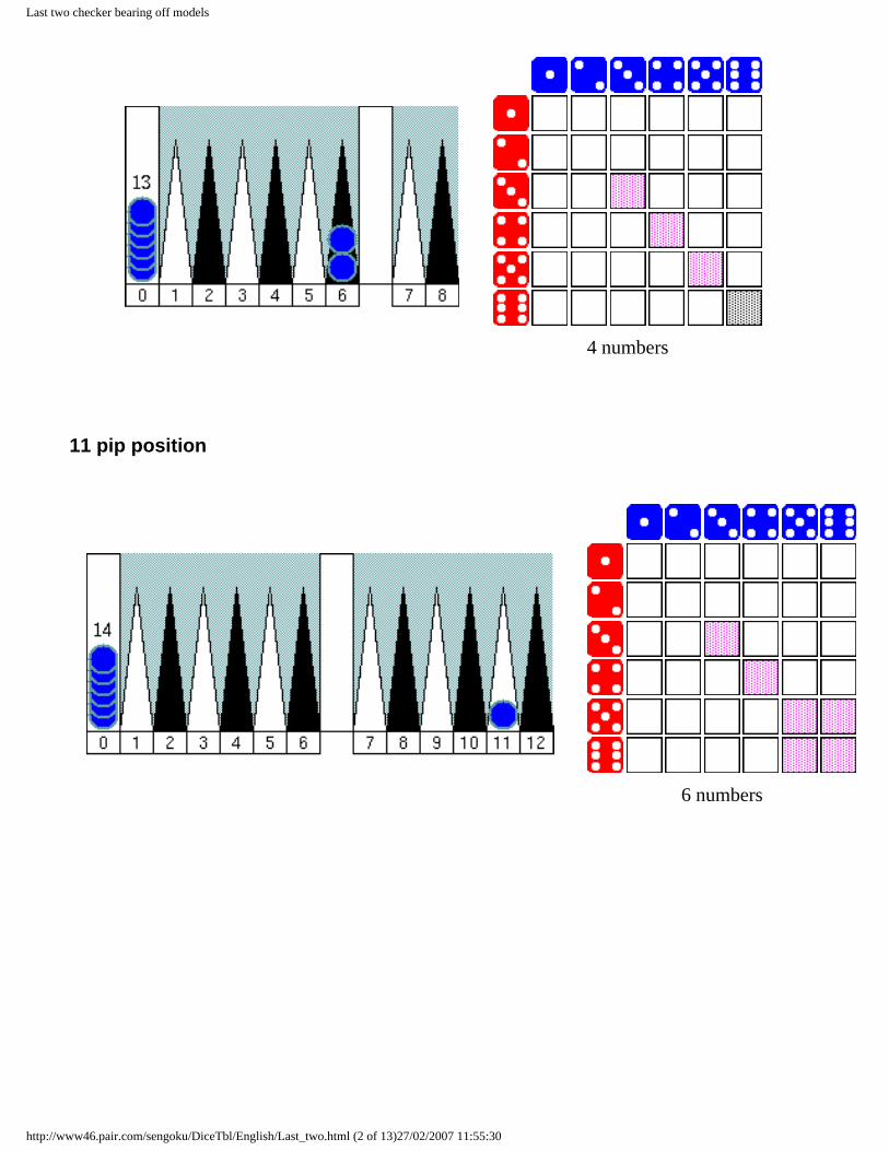
4 numbers
11 pip position
6 numbers
http://www46.pair.com/sengoku/DiceTbl/English/Last_two.html (2 of 13)27/02/2007 11:55:30
Last two checker bearing off models
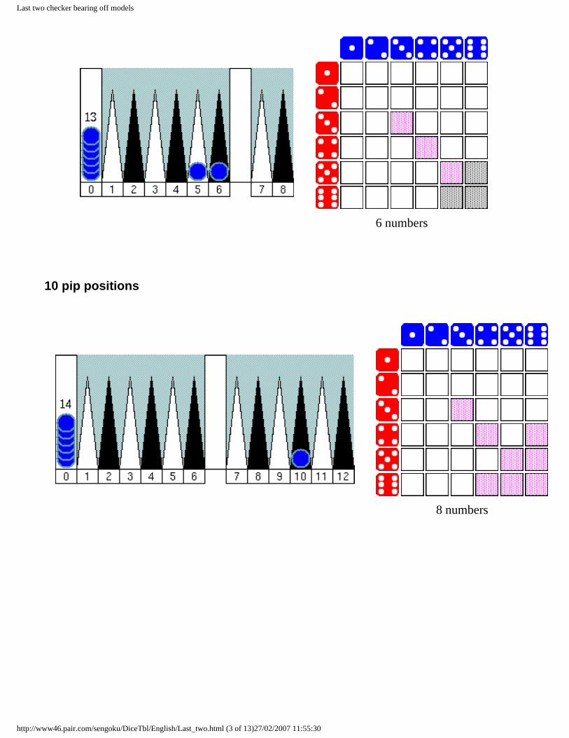
6 numbers
10 pip positions
8 numbers
http://www46.pair.com/sengoku/DiceTbl/English/Last_two.html (3 of 13)27/02/2007 11:55:30
Last two checker bearing off models
8 numbers
6 numbers
9 pip positions
http://www46.pair.com/sengoku/DiceTbl/English/Last_two.html (4 of 13)27/02/2007 11:55:30
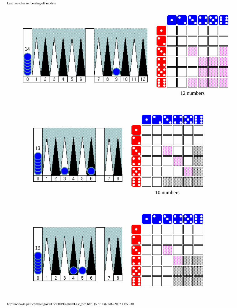
Last two checker bearing off models
12 numbers
10 numbers
http://www46.pair.com/sengoku/DiceTbl/English/Last_two.html (5 of 13)27/02/2007 11:55:30
Last two checker bearing off models
10 numbers
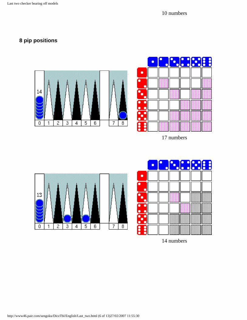
8 pip positions
17 numbers
14 numbers
http://www46.pair.com/sengoku/DiceTbl/English/Last_two.html (6 of 13)27/02/2007 11:55:30
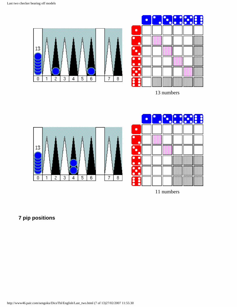
Last two checker bearing off models
13 numbers
11 numbers
7 pip positions
http://www46.pair.com/sengoku/DiceTbl/English/Last_two.html (7 of 13)27/02/2007 11:55:30
Last two checker bearing off models
23 numbers
19 numbers
17 numbers
http://www46.pair.com/sengoku/DiceTbl/English/Last_two.html (8 of 13)27/02/2007 11:55:30
Last two checker bearing off models
15 numbers
6 pip positions
27 numbers
http://www46.pair.com/sengoku/DiceTbl/English/Last_two.html (9 of 13)27/02/2007 11:55:30
Last two checker bearing off models
23 numbers
23 numbers
17 numbers
http://www46.pair.com/sengoku/DiceTbl/English/Last_two.html (10 of 13)27/02/2007 11:55:30
Last two checker bearing off models
5 pip positions
31 numbers
29 numbers
http://www46.pair.com/sengoku/DiceTbl/English/Last_two.html (11 of 13)27/02/2007 11:55:30
Last two checker bearing off models
25 numbers
4 pip positions
34 numbers
http://www46.pair.com/sengoku/DiceTbl/English/Last_two.html (12 of 13)27/02/2007 11:55:30
Last two checker bearing off models
34 numbers
26 numbers
Created by Sho Sengoku
<<Prev Next>> Site top Dice table top
http://www46.pair.com/sengoku/DiceTbl/English/Last_two.html (13 of 13)27/02/2007 11:55:30
Single Direct Shots
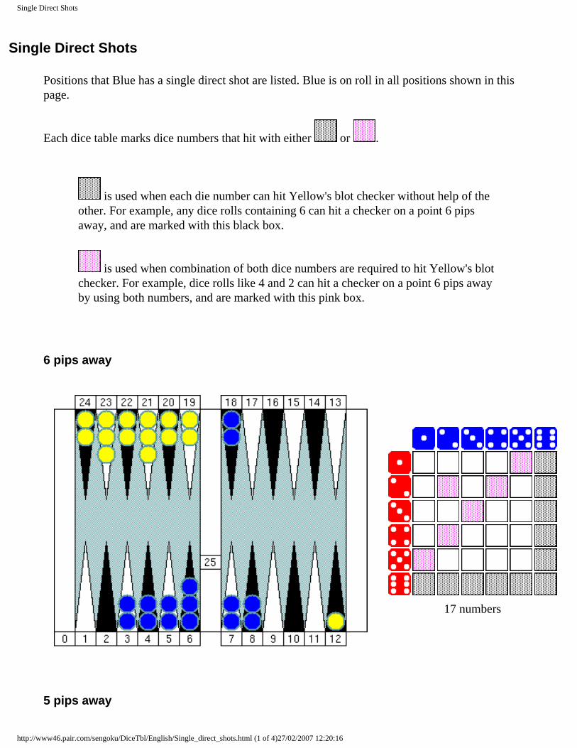
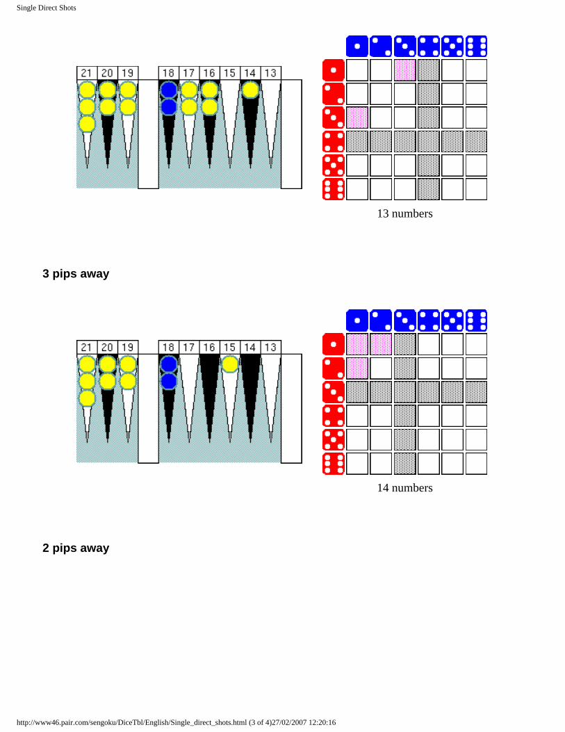
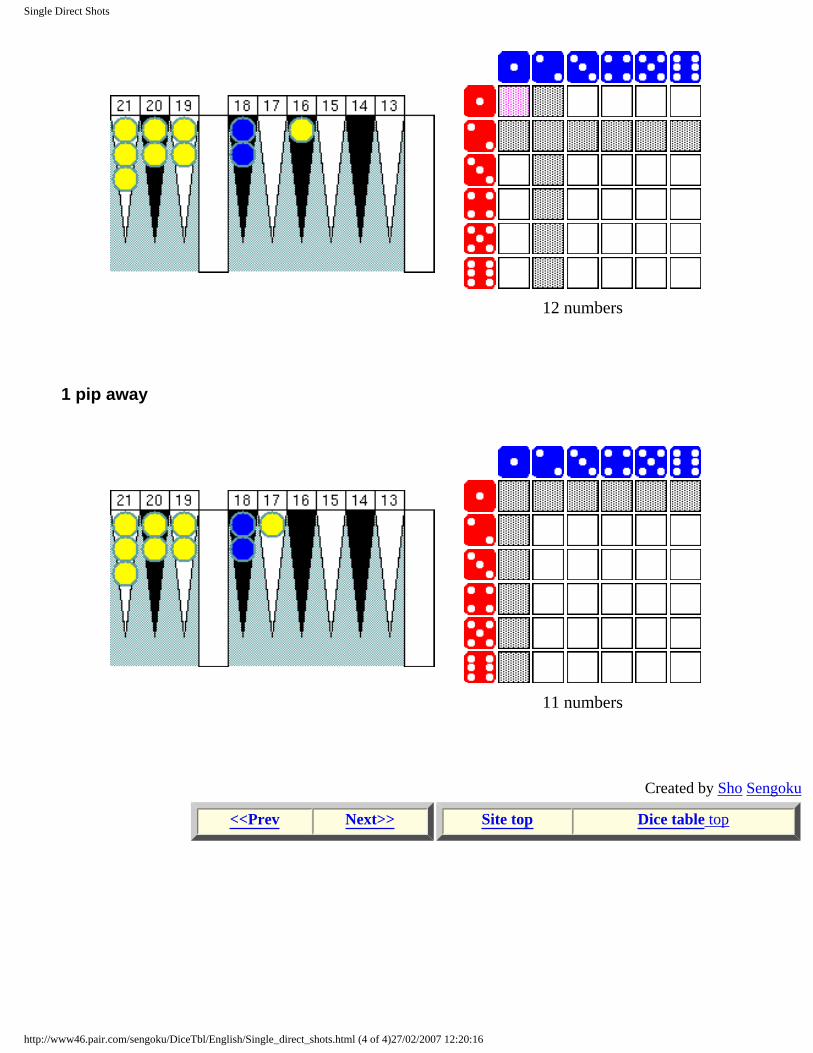
Single Direct Shots
Positions that Blue has a single direct shot are listed. Blue is on roll in all positions shown in this page.
Each dice table marks dice numbers that hit with either or .
is used when each die number can hit Yellow's blot checker without help of the other. For example, any dice rolls containing 6 can hit a checker on a point 6 pips away, and are marked with this black box.
is used when combination of both dice numbers are required to hit Yellow's blot checker. For example, dice rolls like 4 and 2 can hit a checker on a point 6 pips away by using both numbers, and are marked with this pink box.
6 pips away
17 numbers
5 pips away
http://www46.pair.com/sengoku/DiceTbl/English/Single_direct_shots.html (1 of 4)27/02/2007 12:20:16
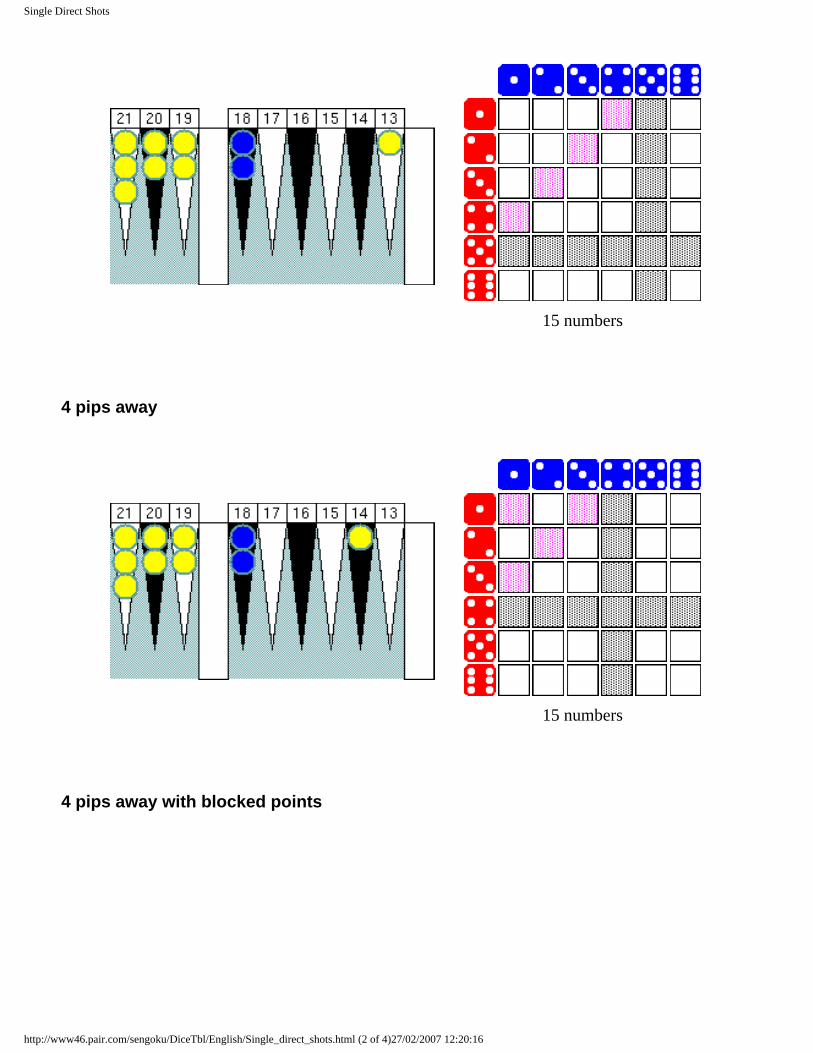
Single Direct Shots
15 numbers
4 pips away
15 numbers
4 pips away with blocked points
http://www46.pair.com/sengoku/DiceTbl/English/Single_direct_shots.html (2 of 4)27/02/2007 12:20:16
Single Direct Shots
13 numbers
3 pips away
14 numbers
2 pips away
http://www46.pair.com/sengoku/DiceTbl/English/Single_direct_shots.html (3 of 4)27/02/2007 12:20:16
Single Direct Shots
12 numbers
1 pip away
11 numbers
Created by Sho Sengoku
<<Prev Next>> Site top Dice table top
http://www46.pair.com/sengoku/DiceTbl/English/Single_direct_shots.html (4 of 4)27/02/2007 12:20:16
Sigle Indirect Shots
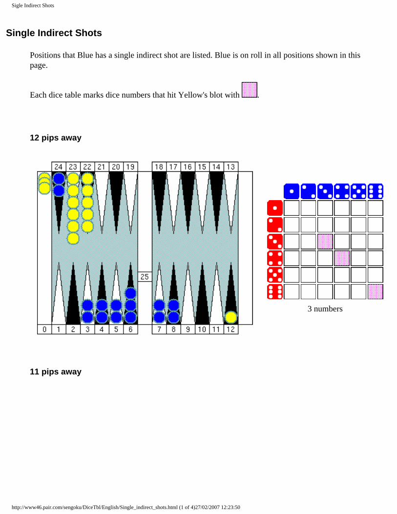
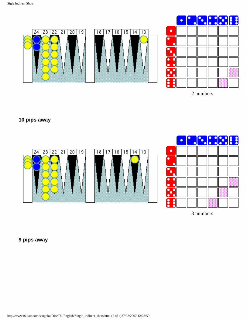
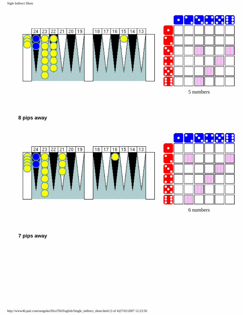
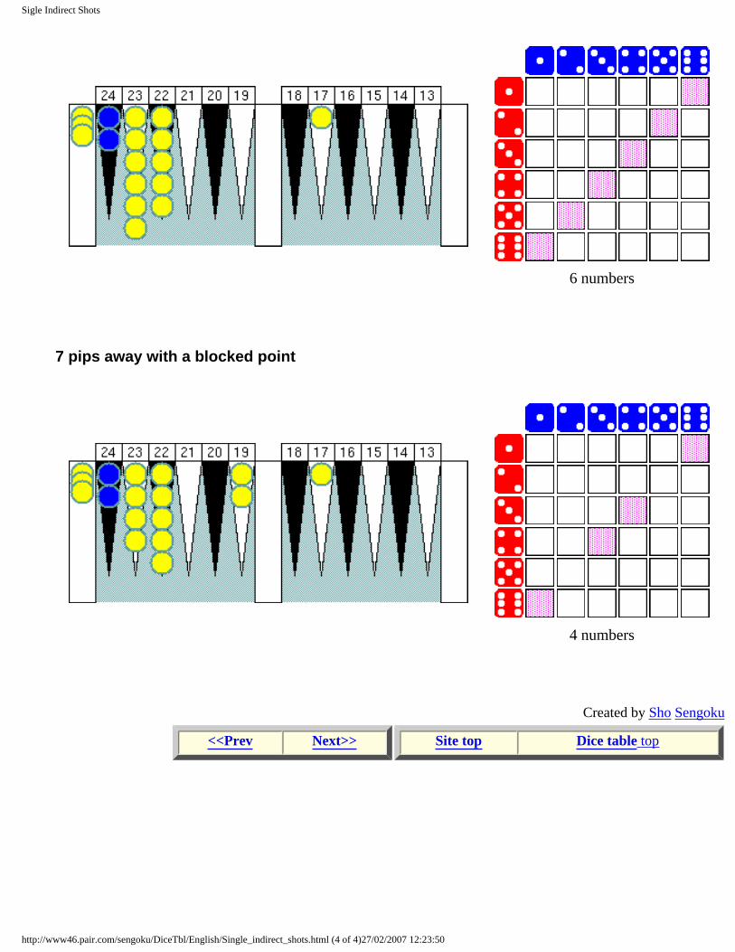
Single Indirect Shots
Positions that Blue has a single indirect shot are listed. Blue is on roll in all positions shown in this page.
Each dice table marks dice numbers that hit Yellow's blot with .
12 pips away
3 numbers
11 pips away
http://www46.pair.com/sengoku/DiceTbl/English/Single_indirect_shots.html (1 of 4)27/02/2007 12:23:50
Sigle Indirect Shots
2 numbers
10 pips away
3 numbers
9 pips away
http://www46.pair.com/sengoku/DiceTbl/English/Single_indirect_shots.html (2 of 4)27/02/2007 12:23:50
Sigle Indirect Shots
5 numbers
8 pips away
6 numbers
7 pips away
http://www46.pair.com/sengoku/DiceTbl/English/Single_indirect_shots.html (3 of 4)27/02/2007 12:23:50
Sigle Indirect Shots
6 numbers
7 pips away with a blocked point
4 numbers
Created by Sho Sengoku
<<Prev Next>> Site top Dice table top
http://www46.pair.com/sengoku/DiceTbl/English/Single_indirect_shots.html (4 of 4)27/02/2007 12:23:50
Double Shots
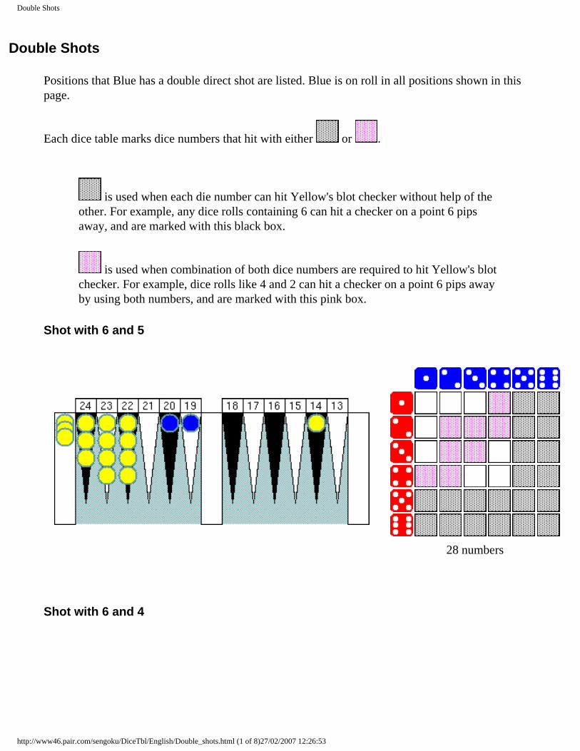
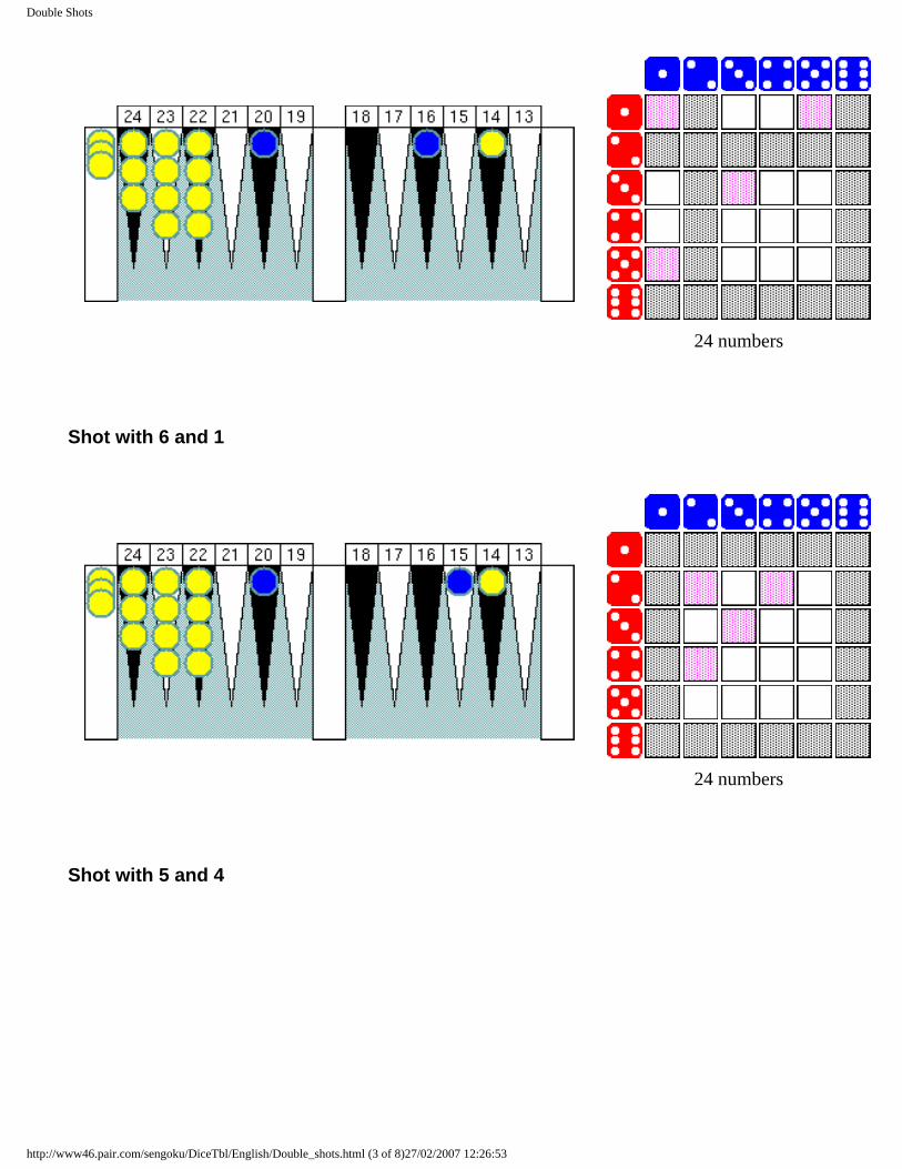
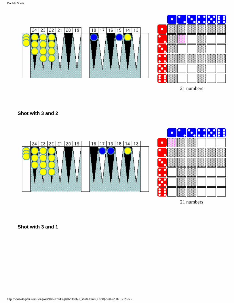
Double Shots
Positions that Blue has a double direct shot are listed. Blue is on roll in all positions shown in this page.
Each dice table marks dice numbers that hit with either or .
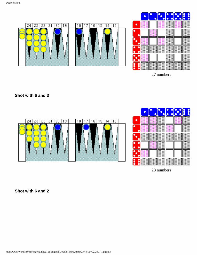
is used when each die number can hit Yellow's blot checker without help of the other. For example, any dice rolls containing 6 can hit a checker on a point 6 pips away, and are marked with this black box.
is used when combination of both dice numbers are required to hit Yellow's blot checker. For example, dice rolls like 4 and 2 can hit a checker on a point 6 pips away by using both numbers, and are marked with this pink box.
Shot with 6 and 5
28 numbers
Shot with 6 and 4
http://www46.pair.com/sengoku/DiceTbl/English/Double_shots.html (1 of 8)27/02/2007 12:26:53
Double Shots
27 numbers
Shot with 6 and 3
28 numbers
Shot with 6 and 2
http://www46.pair.com/sengoku/DiceTbl/English/Double_shots.html (2 of 8)27/02/2007 12:26:53
Double Shots
24 numbers
Shot with 6 and 1
24 numbers
Shot with 5 and 4
http://www46.pair.com/sengoku/DiceTbl/English/Double_shots.html (3 of 8)27/02/2007 12:26:53
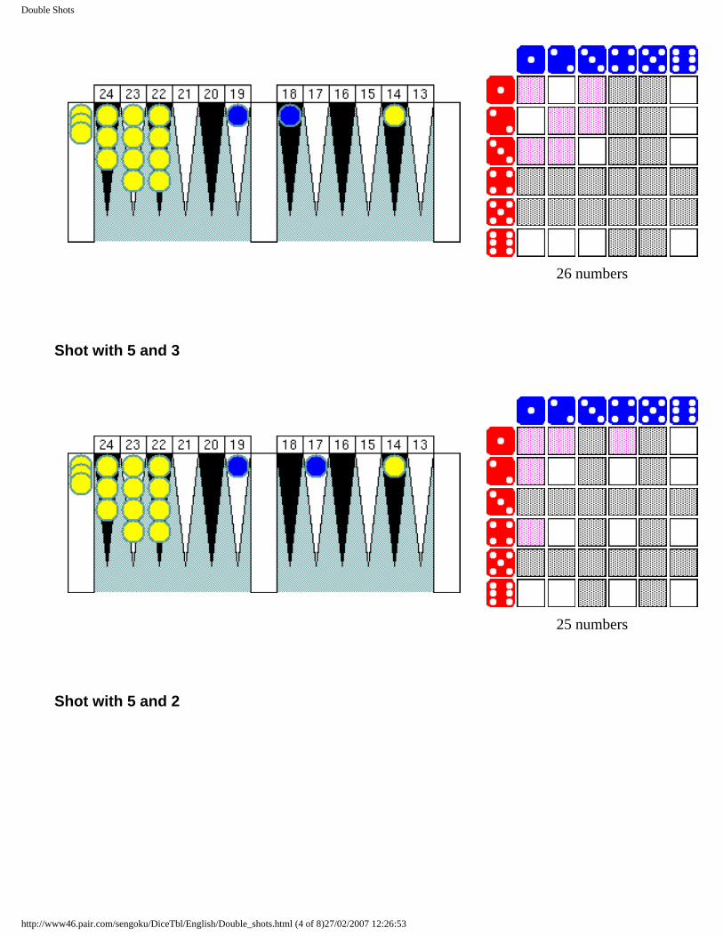
Double Shots
26 numbers
Shot with 5 and 3
25 numbers
Shot with 5 and 2
http://www46.pair.com/sengoku/DiceTbl/English/Double_shots.html (4 of 8)27/02/2007 12:26:53
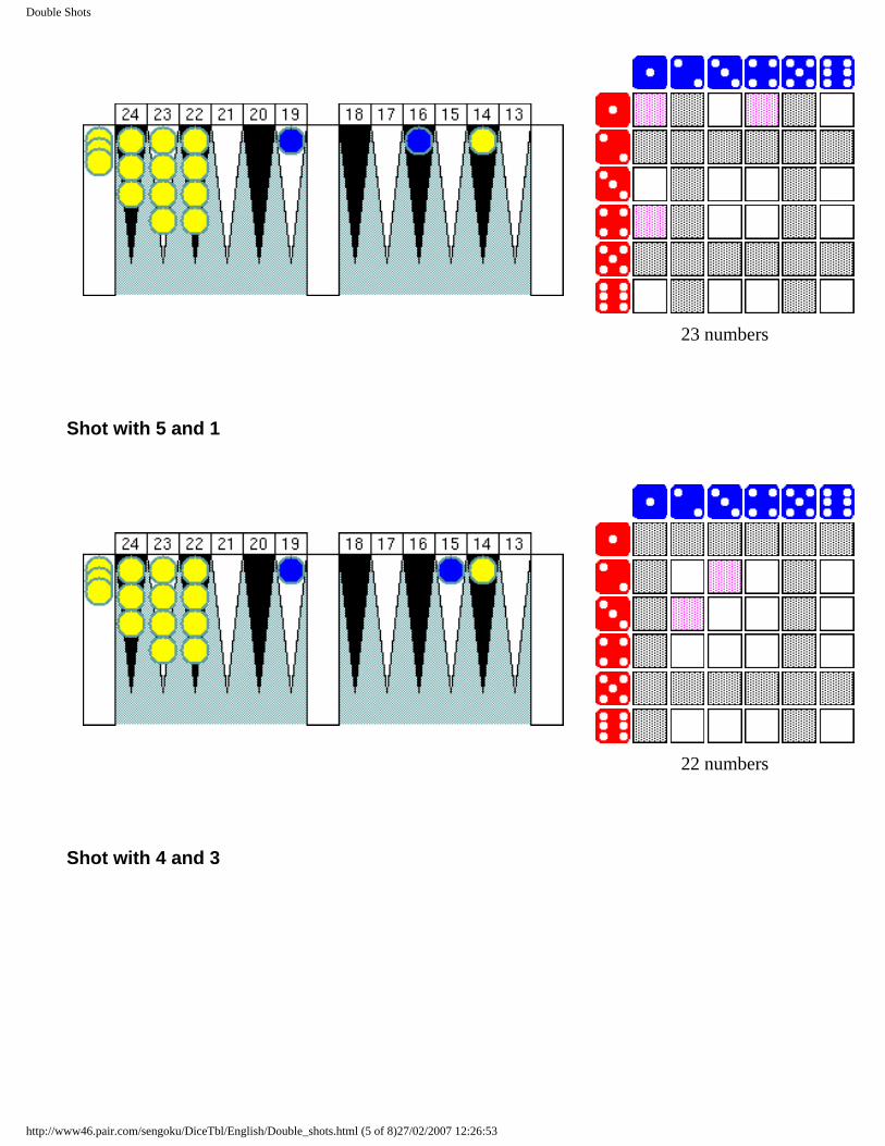
Double Shots
23 numbers
Shot with 5 and 1
22 numbers
Shot with 4 and 3
http://www46.pair.com/sengoku/DiceTbl/English/Double_shots.html (5 of 8)27/02/2007 12:26:53
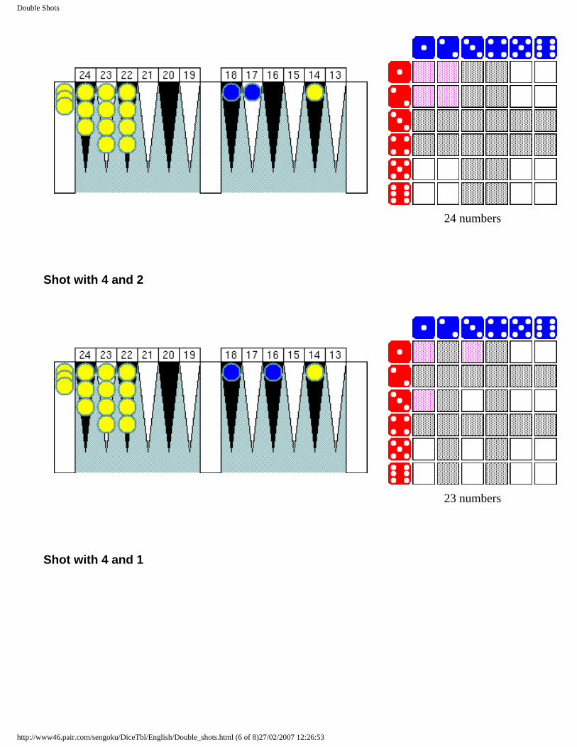
Double Shots
24 numbers
Shot with 4 and 2
23 numbers
Shot with 4 and 1
http://www46.pair.com/sengoku/DiceTbl/English/Double_shots.html (6 of 8)27/02/2007 12:26:53
Double Shots
21 numbers
Shot with 3 and 2
21 numbers
Shot with 3 and 1
http://www46.pair.com/sengoku/DiceTbl/English/Double_shots.html (7 of 8)27/02/2007 12:26:53
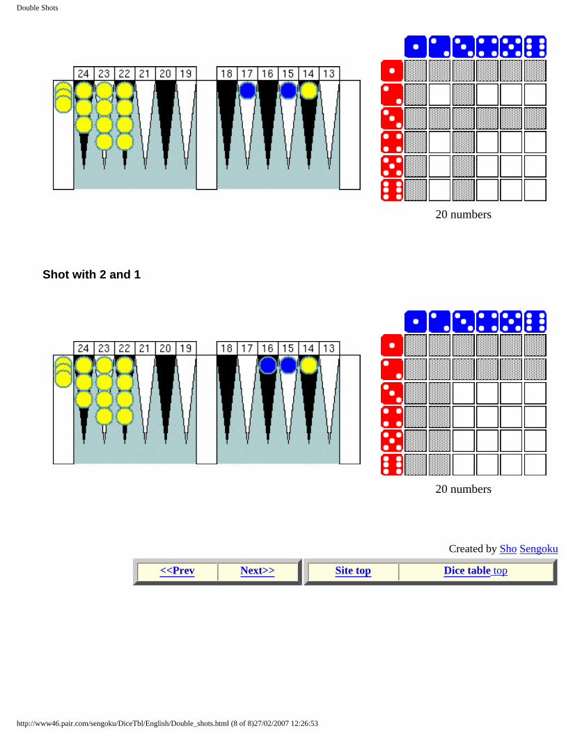
Double Shots
20 numbers
Shot with 2 and 1
20 numbers
Created by Sho Sengoku
<<Prev Next>> Site top Dice table top
http://www46.pair.com/sengoku/DiceTbl/English/Double_shots.html (8 of 8)27/02/2007 12:26:53
http://www-math.bgsu.edu/~albert/m115/probability/outline.html
AN INTRODUCTION TO PROBABILITY
1. What is a probability?
❍ the relative frequency view
❍ the subjective view
2. Measuring probabilities by means of a calibration experiment
3. Interpreting odds
4. Listing all possible outcomes (the sample space)
5. Basic probability rules
6. Equally likely outcomes
7. Constructing a probability table by listing outcomes.
8. Constructing a probability table by simulation
9. Probabilities of "or" and "not" events.
10. An average value of a probability distribution
11. Understanding a two-way table of probabilities
PROBABILITY ACTIVITIES
http://www-math.bgsu.edu/~albert/m115/probability/outline.html (1 of 2)27/02/2007 12:29:57
http://www-math.bgsu.edu/~albert/m115/probability/outline.html
Page Author: Jim Albert (c) [email protected] Document: http://www-math.bgsu.edu/~albert/m115/probability/outline.htmlLast Modified: November 24, 1996
http://www-math.bgsu.edu/~albert/m115/probability/outline.html (2 of 2)27/02/2007 12:29:57
http://www-math.bgsu.edu/~albert/m115/probability/interp.html
INTERPRETING PROBABILITIES
What is a probability? What does it mean to say that a probability of a fair coin is one half, or that the chances I pass this class are 80 percent, or that the probability that the Steelers win the Super Bowl this season is .1?
First, think of some event where the outcome is uncertain. Examples of such outcomes would be the roll of a die, the amount of rain that we get tomorrow, the state of the economy in one month, or who will be the President of the United States in the year 2001. In each case, we don't know for sure what will happen. For example, we don't know exactly how much rain we will get tomorrow.
A probability is a numerical measure of the likelihood of the event. It is a number that we attach to an event, say the event that we'll get over an inch of rain tomorrow, which reflects the likelihood that we will get this much rain.
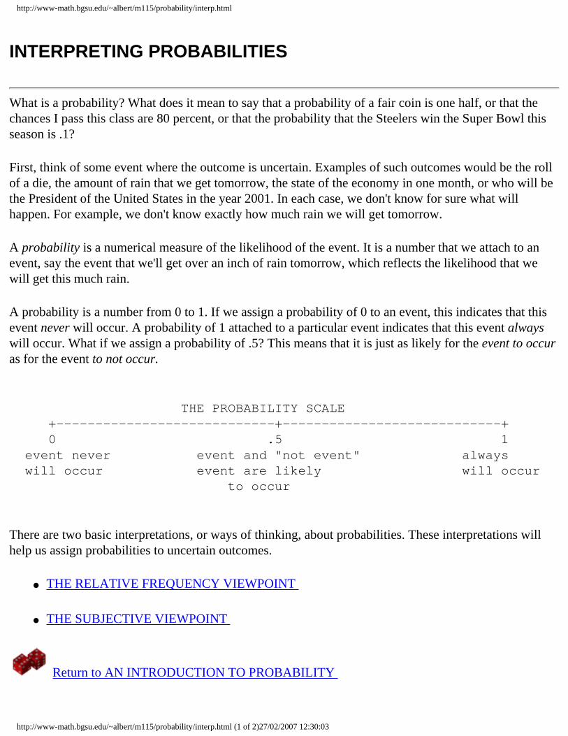
A probability is a number from 0 to 1. If we assign a probability of 0 to an event, this indicates that this event never will occur. A probability of 1 attached to a particular event indicates that this event always will occur. What if we assign a probability of .5? This means that it is just as likely for the event to occur as for the event to not occur.
THE PROBABILITY SCALE +----------------------------+----------------------------+ 0 .5 1 event never event and "not event" always will occur event are likely will occur to occur
There are two basic interpretations, or ways of thinking, about probabilities. These interpretations will help us assign probabilities to uncertain outcomes.
● THE RELATIVE FREQUENCY VIEWPOINT
● THE SUBJECTIVE VIEWPOINT
Return to AN INTRODUCTION TO PROBABILITY
http://www-math.bgsu.edu/~albert/m115/probability/interp.html (1 of 2)27/02/2007 12:30:03

http://www-math.bgsu.edu/~albert/m115/probability/interp.html
Page Author: Jim Albert (© 1996)[email protected] Document: http://www-math.bgsu.edu/~albert/m115/probability/interp.htmlLast Modified: November 18, 1996
http://www-math.bgsu.edu/~albert/m115/probability/interp.html (2 of 2)27/02/2007 12:30:03
http://www-math.bgsu.edu/~albert/m115/probability/relfreq.html
THE RELATIVE FREQUENCY INTERPRETATION OF PROBABILITY
We are interested in learning about the probability of some event in some process. For example, our process could be rolling two dice, and we are interested in the probability in the event that the sum of the numbers on the dice is equal to 6.
Suppose that we can perform this process repeatedly under similar conditions. In our example, suppose that we can roll the two dice many times, where we are careful to roll the dice in the same manner each time.
I did this dice experiment 50 times. Each time I recorded the sum of the two dice and got the following outcomes:
4 10 6 7 5 10 4 6 5 6 11 11 3 3 6 7 10 10 4 4 7 8 8 7 7 4 10 11 3 8 6 10 9 4 8 4 3 8 7 3 7 5 4 11 9 5 5 5 8 5
To approximate the probability that the sum is equal to 6, I count the number of 6's in my experiments (5) and divide by the total number of experiments (50). That is, the probability of observing a 6 is roughly the relative frequency of 6's.
# of 6's PROBABILITY (SUM IS 6) is approximately ----------- # of tosses
5 = ---- = .1 50
In general, the probability of an event can be approximated by the relative frequency , or proportion of times that the event occurs.
http://www-math.bgsu.edu/~albert/m115/probability/relfreq.html (1 of 2)27/02/2007 12:35:42
http://www-math.bgsu.edu/~albert/m115/probability/relfreq.html
# of times event occurs PROBABILITY (EVENT) is approximately ----------------------- # of experiments
Comments about this definition of probability:
1. The observed relative frequency is just an approximation to the true probability of an event. However, if we were able to perform our process more and more times, the relative frequency will eventually approach the actual probability. We could demonstrate this for the dice example. If we tossed the two dice 100 times, 200 times, 300 times, and so on, we would observe that the proportion of 6's would eventually settle down to the true probability of .139.
Click here for a demonstration of this idea using computer dice rolling.
2. This interpretation of probability rests on the important assumption that our process or experiment can be repeated many times under similar circumstances. In the case where this assumption is inappropriate, the subjective interpretation of probability is useful.
Return to AN INTRODUCTION TO PROBABILITY
Page Author: Jim Albert (© 1996)[email protected] Document: http://www-math.bgsu.edu/~albert/m115/probability/relfreq.htmlLast Modified: November 24, 1996
http://www-math.bgsu.edu/~albert/m115/probability/relfreq.html (2 of 2)27/02/2007 12:35:42
http://www-math.bgsu.edu/~albert/m115/probability/dice.html
DEMONSTRATION OF THE RELATIVE FREQUENCY NOTION OF PROBABILITY
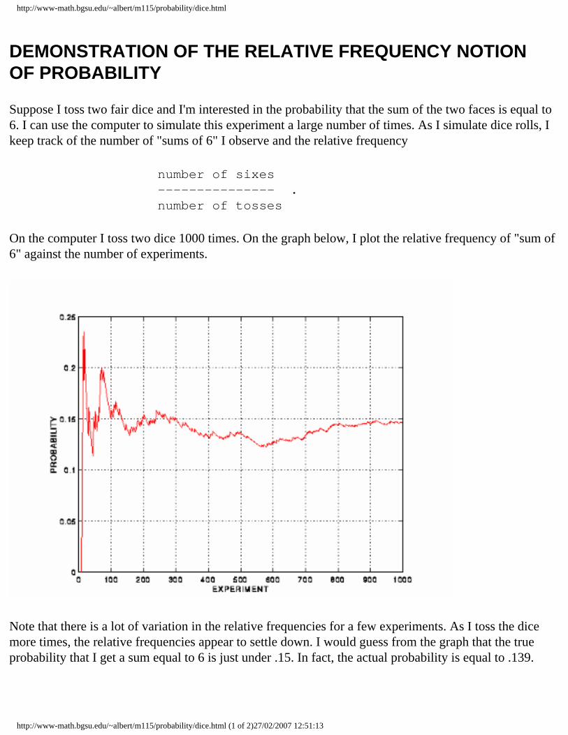
Suppose I toss two fair dice and I'm interested in the probability that the sum of the two faces is equal to 6. I can use the computer to simulate this experiment a large number of times. As I simulate dice rolls, I keep track of the number of "sums of 6" I observe and the relative frequency
number of sixes --------------- . number of tosses
On the computer I toss two dice 1000 times. On the graph below, I plot the relative frequency of "sum of 6" against the number of experiments.
Note that there is a lot of variation in the relative frequencies for a few experiments. As I toss the dice more times, the relative frequencies appear to settle down. I would guess from the graph that the true probability that I get a sum equal to 6 is just under .15. In fact, the actual probability is equal to .139.
http://www-math.bgsu.edu/~albert/m115/probability/dice.html (1 of 2)27/02/2007 12:51:13

http://www-math.bgsu.edu/~albert/m115/probability/dice.html
Return to AN INTRODUCTION TO PROBABILITY
Page Author: Jim Albert (© 1996)[email protected] Document: http://www-math.bgsu.edu/~albert/m115/probability/dice.htmlLast modified: November 24, 1996
http://www-math.bgsu.edu/~albert/m115/probability/dice.html (2 of 2)27/02/2007 12:51:13
http://www-math.bgsu.edu/~albert/m115/probability/subject.html
THE SUBJECTIVE INTERPRETATION OF PROBABILITY
The relative frequency notion of probability is useful when the process of interest, say tossing a coin, can be repeated many times under similar conditions. But we wish to deal with uncertainty of events from processes that will occur a single time. For example, you are likely interested in the probability that you will get an A in this class. You will take this class only one time; even if you retake the class next semester, you won't be taking it under the same conditions as this semester. You'll have a different instructor, a different set of courses, and possibly different work conditions. Similarly, suppose you are interested in the probability that BGSU wins the MAC championship in football next year. There will be only a single football season in question, so it doesn't make sense to talk about the proportion of times BGSU would win the championship under similar conditions.
In the case where the process will happen only one time, how do we view probabilities? Return to our example in which you are interested in the event "get an A in this class". You assign a number to this event (a probability) which reflects your personal belief in the likelihood of this event happening. If you are doing well in this class and you think that an A is a certainty, then you would assign a probability of 1 to this event. If you are experiencing difficulties in the class, you might think "getting an A" is close to an impossibility and so you would assign a probability close to 0. What if you don't know what grade you will get? In this case, you would assign a number to this event between 0 and 1. The use of a calibration experiment is helpful for getting a good measurement at your probability.
Comments about the subjective interpretation of probability:
● A subjective probability reflects a person's opinion about the likelihood of an event. If our event is "Joe will get an A in this class", then my opinion about the likelihood of this event is probably different from Joe's opinion about this event. Probabilities are personal and they will differ between people.
● Can I assign any numbers to events? The numbers you assign must be proper probabilities. That is, they must satisfy some basic rules that all probabilities obey. Also, they should reflect your opinion about the likelihood of the events.
● Assigning subjective probabilities to events seems hard. Yes, it is hard to assign numbers to events, especially when you are uncertain whether the event will occur or not. We will learn more about assigning probabilities by comparing the likelihoods of different events.
Return to AN INTRODUCTION TO PROBABILITY
http://www-math.bgsu.edu/~albert/m115/probability/subject.html (1 of 2)27/02/2007 12:54:31

http://www-math.bgsu.edu/~albert/m115/probability/subject.html
Page Author: Jim Albert (© 1996)[email protected] Document: http://www-math.bgsu.edu/~albert/m115/probability/subject.htmlLast Modified: November 18, 1996
http://www-math.bgsu.edu/~albert/m115/probability/subject.html (2 of 2)27/02/2007 12:54:31
http://www-math.bgsu.edu/~albert/m115/probability/calibration.html
MEASURING PROBABILITIES USING A CALIBRATION EXPERIMENT
Probabilities are generally hard to measure. It is easy to measure probabilities of events that are extremely rare or events that are extremely likely to occur. For example, your probability that the moon is made of green cheese (a rare event) is probably close to 0 and your probability that the sun will rise tomorrow (a sure event) is likely 1. But consider your probability for the event "There will be a white Christmas this year". You can remember years in the past where there was snow on the ground on Christmas. Also you can recall past years with no snow on the ground. So the probability of this event is greater than 0 and less than 1. But how do you obtain the exact probability?
To measure someone's height we need a measuring instrument such as a ruler. Similarly, we need a measuring device for probabilities. This measuring device that we use is called a calibration experiment . This is an experiment which is simple enough so that probabilities of outcomes are easy to specify. In addition, these stated probabilities are objective; you and I would assign the same probabilities to outcomes of this experiment.
The calibration experiment that we use is called a chips-in-bowl experiment. Suppose we have a bowl with a certain number of red chips and white chips. We draw one chip from the bowl at random and we're interested in
Probability(red chip is drawn)
This probability depends on the number of chips in the bowl. If, for example, the bowl contains 1 red chip and 9 white chips, then the probability of choosing a red is 1 out of 10 or 1/10 = .1. If the bowl contains 3 red and 7 chips, then the probability of red is 3/10 = .3. If the bowl contains only red chips (say 10 red and 0 white), then the probability of red is 1. At the other extreme, the probability of red in a bowl with 0 red and 5 white is 0/5 = 0.
Let's return to our event "There will be a white Christmas this year". To help assess its probability, we compare two bets -- one with our event and the second with the event "draw a red chip" from the calibration experiment. This is best illustrated by example. Consider the following two bets:
● BET 1: You get $100 if there is a white Christmas and nothing if there is not a white Christmas.
● BET 2: You get $100 if you draw red in a bowl of 5 red and 5 white and nothing otherwise.
Which bet do you prefer? If you prefer BET 1, then you think that your event of a white Christmas is more likely than the event of drawing red in a bowl with 5 red, 5 white. Since the probability of a red is
http://www-math.bgsu.edu/~albert/m115/probability/calibration.html (1 of 2)27/02/2007 12:59:22
http://www-math.bgsu.edu/~albert/m115/probability/calibration.html
5/10 = .5, this means that your probability of a white Christmas exceeds .5. If you prefer BET 2, then by similar logic, your probability of a white Christmas is smaller than .5.
Say you prefer BET 1 and you know that your probability is larger than .5, or between .5 and 1. To get a better estimate at your probability, you make another comparison of bets, where the second bet has a different number of red and white chips.
Next you compare the two bets
● BET 1: You get $100 if there is a white Christmas and nothing if there is not a white Christmas.
● BET 2: You get $100 if you draw red in a bowl of 7 red and 3 white and nothing otherwise.
Suppose that you prefer BET 2. Since the probability of red in a bowl of 7 red and 3 white is 7/10 = .7, this means that your probability of a white Christmas must be smaller than .7.
We've now made two judgements between bets. The first judgement told us that our probability of white Christmas was greater than .5 and the second judgement told us that our probability was smaller than .7. What is our probability? We don't know the exact value yet, but we know that it must fall between .5 and.7. We can represent our probability by an interval of values on a number line.
OUR PROBABILITY OF WHITE CHRISTMAS LIES IN HERE:
********* +----+----+----+----+----+----+----+----+----+----+ 0 .1 .2 .3 .4 .5 .6 .7 .8 .9 1
What if we wanted to get a more accurate estimate at our probability? We need to make more comparison between bets. For example, we could compare two bets, where the first bet used our event and the second used the event "draw red" from a bowl of chips with 6 red and 4 white. After a number of these comparisons, we can get a pretty accurate estimate at our probability.
Return to AN INTRODUCTION TO PROBABILITY
Page Author: Jim Albert (© 1996) [email protected] Document: http://www-math.bgsu.edu/~albert/m115/probability/calibration.htmlLast Modified: November 24, 1996
http://www-math.bgsu.edu/~albert/m115/probability/calibration.html (2 of 2)27/02/2007 12:59:22
http://www-math.bgsu.edu/~albert/m115/probability/odds.html
INTERPRETING ODDS
Often probabilities are stated in the media in terms of odds. For example, the following is a paragraph from Roxy Roxborough's Odds and Ends column in USA Today .
EYE OF THE TIGER: Sensational PGA tour rookie Tiger Woods has been installed an early 9-5 favorite to win the most cash at the Skins Game at the Rancho La Quinta Golf Course in La Quinta, Calif., Nov. 30-Dec. 1. The charismatic Woods will have to contend with Fred Couples, the close 2-1 second choice, as well as the still dangerous Tom Watson, 3-1, and power stroker John Daly, 9-2.
We read that Tiger Woods is the favorite to win this golf tournament at a 9-5 odds. What does this mean?
An odds of an event is the ratio of the probability that the event will not occur to the probability that the event will occur . In our example, the event is "Tiger Woods will win". We read that the odds of this event are 9 to 5 or 9/5. This means that
Probability (Tiger Woods will not win) 9 -------------------------------------- = --- Probability (Tiger Wodds will win) 5
This means that it is more likely for Woods to lose the tournament than win the tournament.
How can we convert odds to probabilities? There is a simple recipe. If the odds of an event are stated as A to B (or A-B or A/B), then the probability of the event is
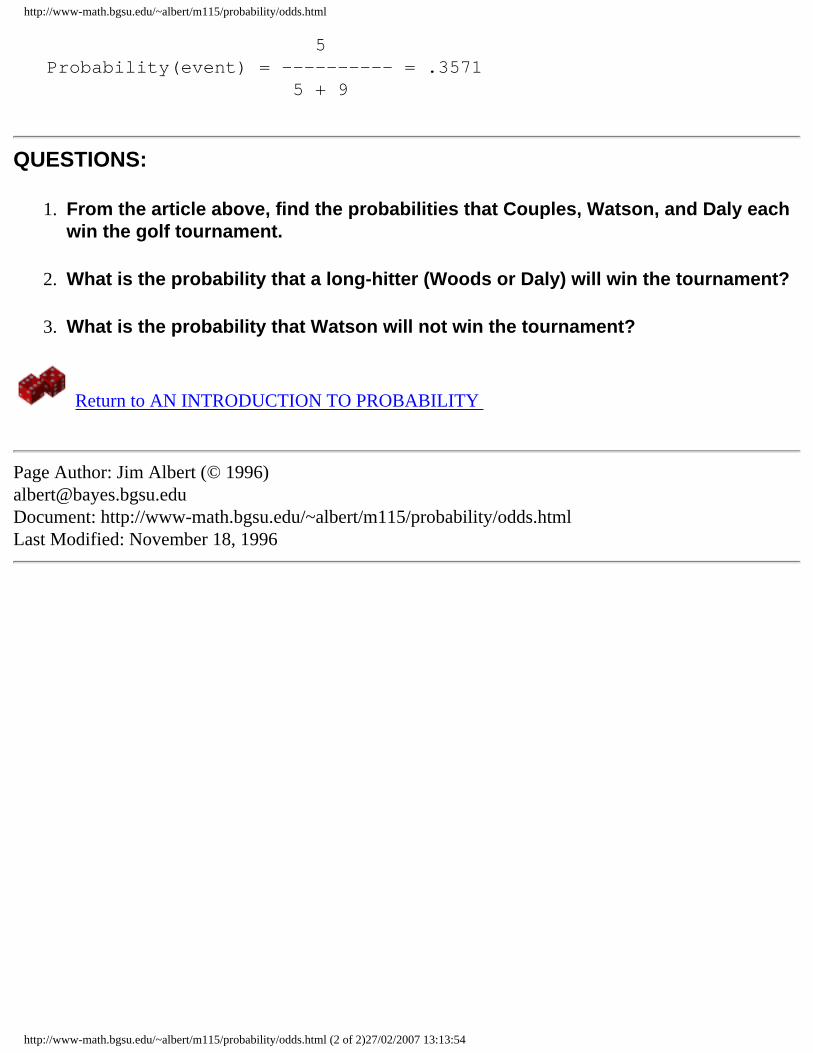
B Probability(event) = ---------- B + A
So, for example, if the odds of Woods winning are 9-5 or 9/5, then the probability of Woods winning is
http://www-math.bgsu.edu/~albert/m115/probability/odds.html (1 of 2)27/02/2007 13:13:54
http://www-math.bgsu.edu/~albert/m115/probability/odds.html
5 Probability(event) = ---------- = .3571 5 + 9
QUESTIONS:
1. From the article above, find the probabilities that Couples, Watson, and Daly each win the golf tournament.
2. What is the probability that a long-hitter (Woods or Daly) will win the tournament?
3. What is the probability that Watson will not win the tournament?
Return to AN INTRODUCTION TO PROBABILITY
Page Author: Jim Albert (© 1996)[email protected] Document: http://www-math.bgsu.edu/~albert/m115/probability/odds.htmlLast Modified: November 18, 1996
http://www-math.bgsu.edu/~albert/m115/probability/odds.html (2 of 2)27/02/2007 13:13:54
http://www-math.bgsu.edu/~albert/m115/probability/sample_space.html
LISTING ALL POSSIBLE OUTCOMES (THE SAMPLE SPACE)
Suppose that we will observe some process or experiment in which the outcome is not known in advance. For example, suppose we plan to roll two dice and we're interested in the sum of the two numbers appearing on the top faces. Before we can talk about probabilities of various sums, say 3 or 7, we have to understand what outcomes are possible in this experiment.
If we roll two dice, each die could show 1, 2, 3, 4, 5, 6. So the sum of the two faces could be any whole number from 2 to 12. We call this set of possible outcomes in the random experiment the sample space . Here the sample space can be written as
Sample space = {2, 3, 4, 5, 6, 7, 8, 9, 10, 11, 12}
Let's consider the set of all possible outcomes for other basic random experiments. Suppose we plan to toss a coin 3 times and the outcome of interest is the number of heads. The sample space in this case is the different numbers of heads you could get if you toss a coin three times. Here you could get 0 heads, 1 heads, 2 heads or 3 heads, so we write the sample space as
Sample space = {0, 1, 2, 3}
Don't forget to include the outcome 0 -- if we toss a coin three times and get all tails, then the number of heads is equal to 0.
The concept of a sample space is also relevant for experiments where the outcomes are non-numerical. Suppose I draw a card from a standard deck of playing cards. If I'm interested in the suit of the card, there are four possible outcomes and the sample space is
Sample space = {Spade, Heart, Diamond, Club}
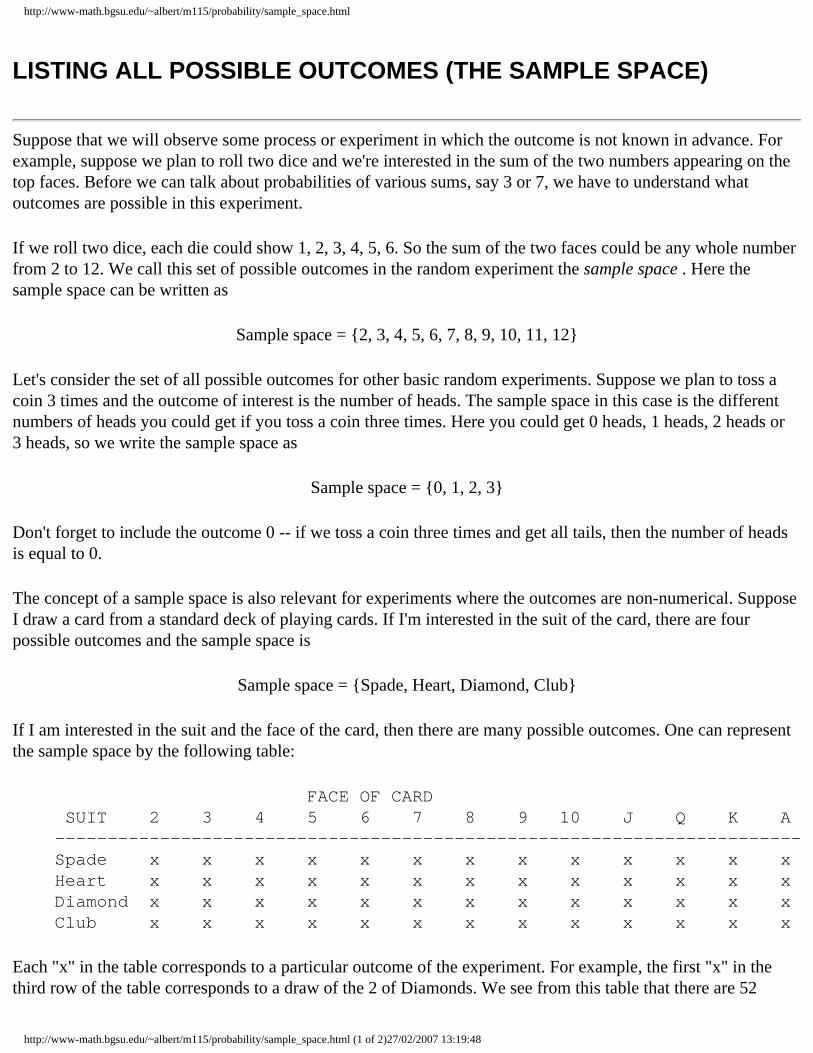
If I am interested in the suit and the face of the card, then there are many possible outcomes. One can represent the sample space by the following table:
FACE OF CARD SUIT 2 3 4 5 6 7 8 9 10 J Q K A ----------------------------------------------------------------------- Spade x x x x x x x x x x x x x Heart x x x x x x x x x x x x x Diamond x x x x x x x x x x x x x Club x x x x x x x x x x x x x
Each "x" in the table corresponds to a particular outcome of the experiment. For example, the first "x" in the third row of the table corresponds to a draw of the 2 of Diamonds. We see from this table that there are 52
http://www-math.bgsu.edu/~albert/m115/probability/sample_space.html (1 of 2)27/02/2007 13:19:48

http://www-math.bgsu.edu/~albert/m115/probability/sample_space.html
possible outcomes.
Once we understand what the collection of all possible outcomes looks like, we can think about assigning probabilities to the different outcomes. But be careful -- incorrect probability assignments can be made because in mistakes in specifying the entire sample space.
Return to AN INTRODUCTION TO PROBABILITY
Page Author: Jim Albert (©1996) [email protected] Document: http://www-math.bgsu.edu/~albert/m115/probability/sample_space.html Last Modified: January 21 1998
http://www-math.bgsu.edu/~albert/m115/probability/sample_space.html (2 of 2)27/02/2007 13:19:48
http://www-math.bgsu.edu/~albert/m115/probability/prob_rules.html
PROBABILITY RULES
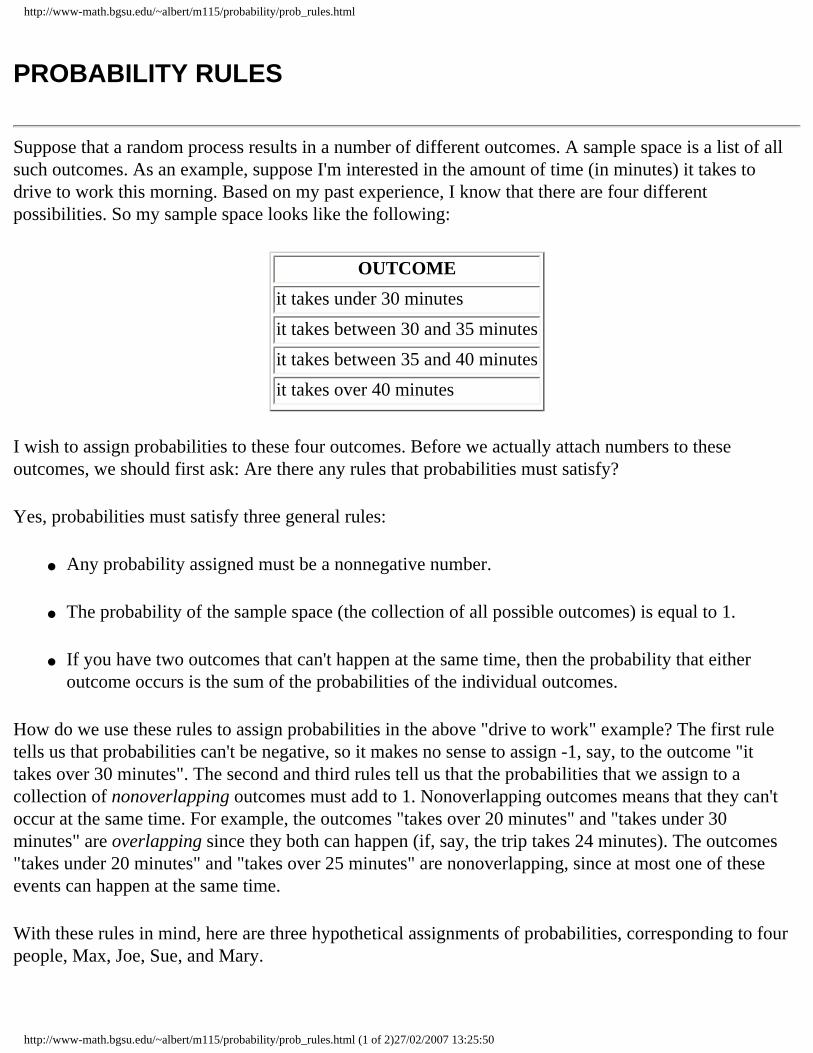
Suppose that a random process results in a number of different outcomes. A sample space is a list of all such outcomes. As an example, suppose I'm interested in the amount of time (in minutes) it takes to drive to work this morning. Based on my past experience, I know that there are four different possibilities. So my sample space looks like the following:
OUTCOME
it takes under 30 minutes
it takes between 30 and 35 minutes
it takes between 35 and 40 minutes
it takes over 40 minutes
I wish to assign probabilities to these four outcomes. Before we actually attach numbers to these outcomes, we should first ask: Are there any rules that probabilities must satisfy?
Yes, probabilities must satisfy three general rules:
● Any probability assigned must be a nonnegative number.
● The probability of the sample space (the collection of all possible outcomes) is equal to 1.
● If you have two outcomes that can't happen at the same time, then the probability that either outcome occurs is the sum of the probabilities of the individual outcomes.
How do we use these rules to assign probabilities in the above "drive to work" example? The first rule tells us that probabilities can't be negative, so it makes no sense to assign -1, say, to the outcome "it takes over 30 minutes". The second and third rules tell us that the probabilities that we assign to a collection of nonoverlapping outcomes must add to 1. Nonoverlapping outcomes means that they can't occur at the same time. For example, the outcomes "takes over 20 minutes" and "takes under 30 minutes" are overlapping since they both can happen (if, say, the trip takes 24 minutes). The outcomes "takes under 20 minutes" and "takes over 25 minutes" are nonoverlapping, since at most one of these events can happen at the same time.
With these rules in mind, here are three hypothetical assignments of probabilities, corresponding to four people, Max, Joe, Sue, and Mary.
http://www-math.bgsu.edu/~albert/m115/probability/prob_rules.html (1 of 2)27/02/2007 13:25:50
http://www-math.bgsu.edu/~albert/m115/probability/prob_rules.html
FOUR SETS OF PROBABILITIES
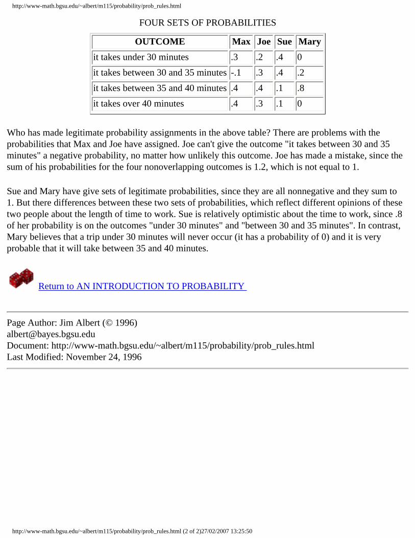
OUTCOME Max Joe Sue Mary
it takes under 30 minutes .3 .2 .4 0
it takes between 30 and 35 minutes -.1 .3 .4 .2
it takes between 35 and 40 minutes .4 .4 .1 .8
it takes over 40 minutes .4 .3 .1 0
Who has made legitimate probability assignments in the above table? There are problems with the probabilities that Max and Joe have assigned. Joe can't give the outcome "it takes between 30 and 35 minutes" a negative probability, no matter how unlikely this outcome. Joe has made a mistake, since the sum of his probabilities for the four nonoverlapping outcomes is 1.2, which is not equal to 1.
Sue and Mary have give sets of legitimate probabilities, since they are all nonnegative and they sum to 1. But there differences between these two sets of probabilities, which reflect different opinions of these two people about the length of time to work. Sue is relatively optimistic about the time to work, since .8 of her probability is on the outcomes "under 30 minutes" and "between 30 and 35 minutes". In contrast, Mary believes that a trip under 30 minutes will never occur (it has a probability of 0) and it is very probable that it will take between 35 and 40 minutes.
Return to AN INTRODUCTION TO PROBABILITY
Page Author: Jim Albert (© 1996) [email protected] Document: http://www-math.bgsu.edu/~albert/m115/probability/prob_rules.html Last Modified: November 24, 1996
http://www-math.bgsu.edu/~albert/m115/probability/prob_rules.html (2 of 2)27/02/2007 13:25:50
http://www-math.bgsu.edu/~albert/m115/probability/equally_likely.html
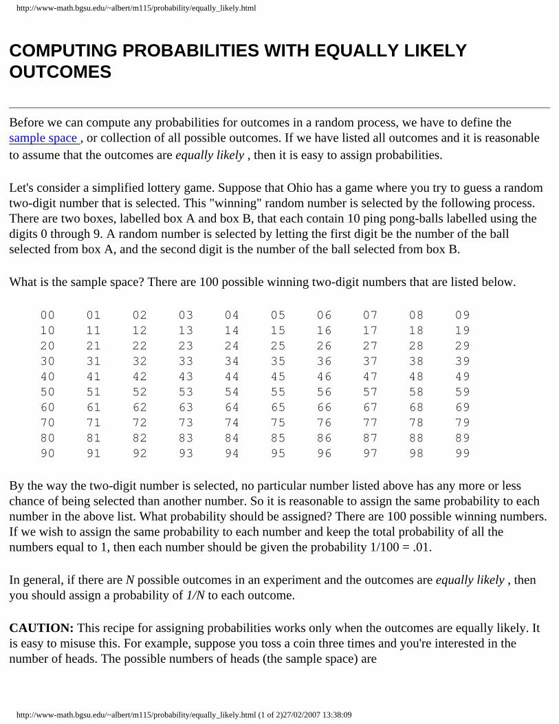
COMPUTING PROBABILITIES WITH EQUALLY LIKELY OUTCOMES
Before we can compute any probabilities for outcomes in a random process, we have to define the sample space , or collection of all possible outcomes. If we have listed all outcomes and it is reasonable to assume that the outcomes are equally likely , then it is easy to assign probabilities.
Let's consider a simplified lottery game. Suppose that Ohio has a game where you try to guess a random two-digit number that is selected. This "winning" random number is selected by the following process. There are two boxes, labelled box A and box B, that each contain 10 ping pong-balls labelled using the digits 0 through 9. A random number is selected by letting the first digit be the number of the ball selected from box A, and the second digit is the number of the ball selected from box B.
What is the sample space? There are 100 possible winning two-digit numbers that are listed below.
00 01 02 03 04 05 06 07 08 09 10 11 12 13 14 15 16 17 18 19 20 21 22 23 24 25 26 27 28 29 30 31 32 33 34 35 36 37 38 39 40 41 42 43 44 45 46 47 48 49 50 51 52 53 54 55 56 57 58 59 60 61 62 63 64 65 66 67 68 69 70 71 72 73 74 75 76 77 78 79 80 81 82 83 84 85 86 87 88 89 90 91 92 93 94 95 96 97 98 99
By the way the two-digit number is selected, no particular number listed above has any more or less chance of being selected than another number. So it is reasonable to assign the same probability to each number in the above list. What probability should be assigned? There are 100 possible winning numbers. If we wish to assign the same probability to each number and keep the total probability of all the numbers equal to 1, then each number should be given the probability 1/100 = .01.
In general, if there are N possible outcomes in an experiment and the outcomes are equally likely , then you should assign a probability of 1/N to each outcome.
CAUTION: This recipe for assigning probabilities works only when the outcomes are equally likely. It is easy to misuse this. For example, suppose you toss a coin three times and you're interested in the number of heads. The possible numbers of heads (the sample space) are
http://www-math.bgsu.edu/~albert/m115/probability/equally_likely.html (1 of 2)27/02/2007 13:38:09
http://www-math.bgsu.edu/~albert/m115/probability/equally_likely.html
0 head, 1 head, 2 heads, 3 heads
There are four outcomes in this case. But it is incorrect to assume that the probabilities of each outcome is 1/4 = .25. These four outcomes are not equally likely. In fact, the probability of 1 head is three times the probability of 3 heads.
Return to AN INTRODUCTION TO PROBABILITY
Page Author: Jim Albert (© 1996)[email protected] Document: http://www-math.bgsu.edu/~albert/m115/probability/equally_likely.htmlLast Modified: November 18, 1996
http://www-math.bgsu.edu/~albert/m115/probability/equally_likely.html (2 of 2)27/02/2007 13:38:09
http://www-math.bgsu.edu/~albert/m115/probability/prob_list.html
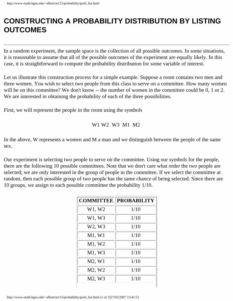
CONSTRUCTING A PROBABILITY DISTRIBUTION BY LISTING OUTCOMES
In a random experiment, the sample space is the collection of all possible outcomes. In some situations, it is reasonable to assume that all of the possible outcomes of the experiment are equally likely. In this case, it is straightforward to compute the probability distribution for some variable of interest.
Let us illustrate this construction process for a simple example. Suppose a room contains two men and three women. You wish to select two people from this class to serve on a committee. How many women will be on this committee? We don't know -- the number of women in the committee could be 0, 1 or 2. We are interested in obtaining the probability of each of the three possibilities.
First, we will represent the people in the room using the symbols
W1 W2 W3 M1 M2
In the above, W represents a women and M a man and we distinguish between the people of the same sex.
Our experiment is selecting two people to serve on the committee. Using our symbols for the people, there are the following 10 possible committees. Note that we don't care what order the two people are selected; we are only interested in the group of people in the committee. If we select the committee at random, then each possible group of two people has the same chance of being selected. Since there are 10 groups, we assign to each possible committee the probability 1/10.
COMMITTEE PROBABILITY
W1, W2 1/10
W1, W3 1/10
W2, W3 1/10
M1, W1 1/10
M1, W2 1/10
M1, W3 1/10
M2, W1 1/10
M2, W2 1/10
M2, W3 1/10
http://www-math.bgsu.edu/~albert/m115/probability/prob_list.html (1 of 3)27/02/2007 13:41:51
http://www-math.bgsu.edu/~albert/m115/probability/prob_list.html
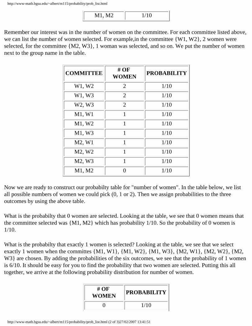
M1, M2 1/10
Remember our interest was in the number of women on the committee. For each committee listed above, we can list the number of women selected. For example,in the committee {W1, W2}, 2 women were selected, for the committee {M2, W3}, 1 woman was selected, and so on. We put the number of women next to the group name in the table.
COMMITTEE # OF
WOMEN PROBABILITY
W1, W2 2 1/10
W1, W3 2 1/10
W2, W3 2 1/10
M1, W1 1 1/10
M1, W2 1 1/10
M1, W3 1 1/10
M2, W1 1 1/10
M2, W2 1 1/10
M2, W3 1 1/10
M1, M2 0 1/10
Now we are ready to construct our probabilty table for "number of women". In the table below, we list all possible numbers of women we could pick (0, 1 or 2). Then we assign probabilities to the three outcomes by using the above table.
What is the probabilty that 0 women are selected. Looking at the table, we see that 0 women means that the committee selected was {M1, M2} which has probability 1/10. So the probability of 0 women is 1/10.
What is the probabilty that exactly 1 women is selected? Looking at the table, we see that we select exactly 1 women when the committes {M1, W1}, {M1, W2}, {M1, W3}, {M2, W1}, {M2, W2}, {M2, W3} are chosen. By adding the probabilities of the six outcomes, we see that the probability of 1 women is 6/10. It should be easy for you to find the probability that two women are selected. Putting this all together, we arrive at the following probability distribution for number of women.
# OF WOMEN
PROBABILITY
0 1/10
http://www-math.bgsu.edu/~albert/m115/probability/prob_list.html (2 of 3)27/02/2007 13:41:51

http://www-math.bgsu.edu/~albert/m115/probability/prob_list.html
1 6/10
2 3/10
Return to AN INTRODUCTION TO PROBABILITY
Page Author: Jim Albert (© 1996) [email protected] Document: http://www-math.bgsu.edu/~albert/m115/probability/prob_list.html Last Modified: November 24, 1996
http://www-math.bgsu.edu/~albert/m115/probability/prob_list.html (3 of 3)27/02/2007 13:41:51
http://www-math.bgsu.edu/~albert/m115/probability/prob_simulate.html
CONSTRUCTING A PROBABILITY DISTRIBUTION BY SIMULATION
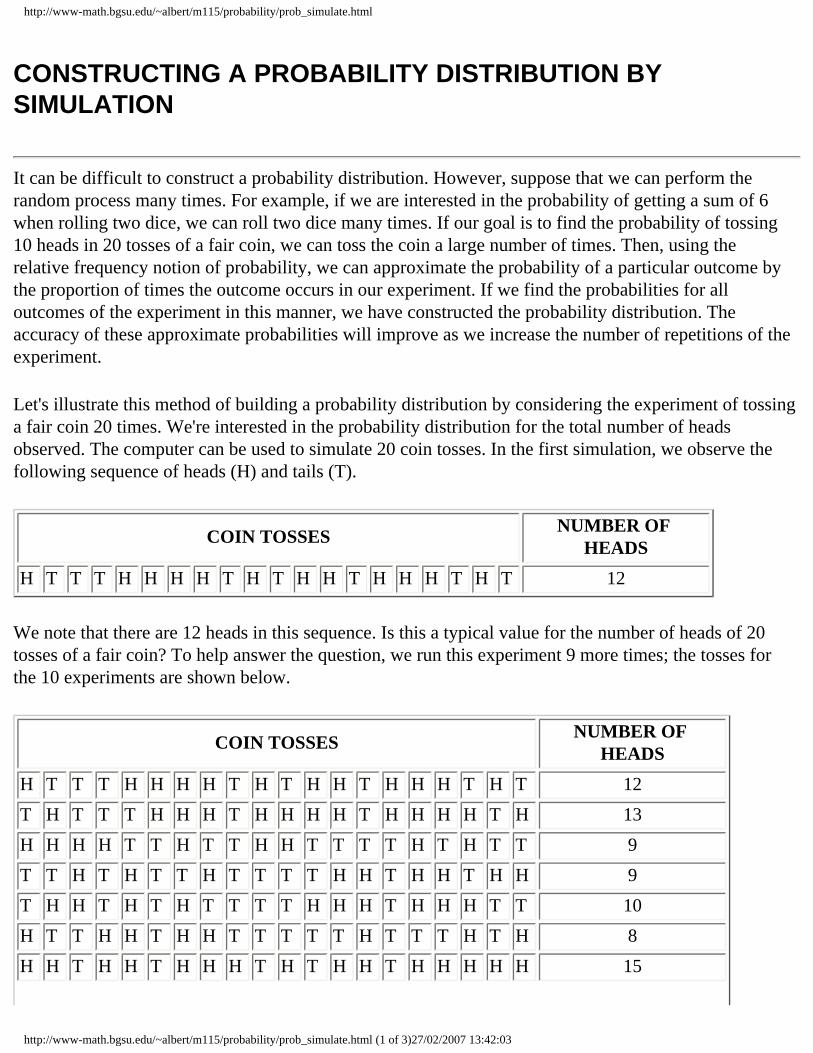
It can be difficult to construct a probability distribution. However, suppose that we can perform the random process many times. For example, if we are interested in the probability of getting a sum of 6 when rolling two dice, we can roll two dice many times. If our goal is to find the probability of tossing 10 heads in 20 tosses of a fair coin, we can toss the coin a large number of times. Then, using the relative frequency notion of probability, we can approximate the probability of a particular outcome by the proportion of times the outcome occurs in our experiment. If we find the probabilities for all outcomes of the experiment in this manner, we have constructed the probability distribution. The accuracy of these approximate probabilities will improve as we increase the number of repetitions of the experiment.
Let's illustrate this method of building a probability distribution by considering the experiment of tossing a fair coin 20 times. We're interested in the probability distribution for the total number of heads observed. The computer can be used to simulate 20 coin tosses. In the first simulation, we observe the following sequence of heads (H) and tails (T).
COIN TOSSES NUMBER OF
HEADS
H T T T H H H H T H T H H T H H H T H T 12
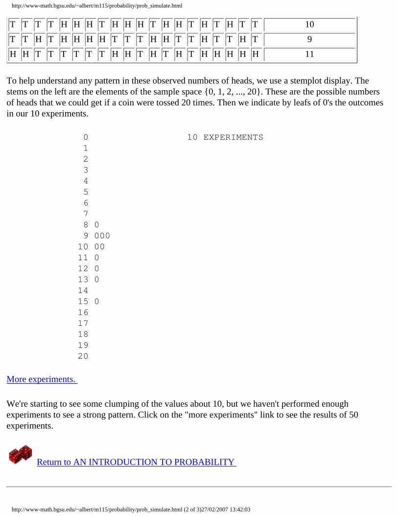
We note that there are 12 heads in this sequence. Is this a typical value for the number of heads of 20 tosses of a fair coin? To help answer the question, we run this experiment 9 more times; the tosses for the 10 experiments are shown below.
COIN TOSSES NUMBER OF
HEADS
H T T T H H H H T H T H H T H H H T H T 12
T H T T T H H H T H H H H T H H H H T H 13
H H H H T T H T T H H T T T T H T H T T 9
T T H T H T T H T T T T H H T H H T H H 9
T H H T H T H T T T T H H H T H H H T T 10
H T T H H T H H T T T T T H T T T H T H 8
H H T H H T H H H T H T H H T H H H H H 15
http://www-math.bgsu.edu/~albert/m115/probability/prob_simulate.html (1 of 3)27/02/2007 13:42:03
http://www-math.bgsu.edu/~albert/m115/probability/prob_simulate.html
T T T T H H H T H H H T H H T H T H T T 10
T T H T H H H H T T T H H T T H T T H T 9
H H T T T T T T H H T H T H T H H H H H 11
To help understand any pattern in these observed numbers of heads, we use a stemplot display. The stems on the left are the elements of the sample space {0, 1, 2, ..., 20}. These are the possible numbers of heads that we could get if a coin were tossed 20 times. Then we indicate by leafs of 0's the outcomes in our 10 experiments.
0 10 EXPERIMENTS 1 2 3 4 5 6 7 8 0 9 000 10 00 11 0 12 0 13 0 14 15 0 16 17 18 19 20
More experiments.
We're starting to see some clumping of the values about 10, but we haven't performed enough experiments to see a strong pattern. Click on the "more experiments" link to see the results of 50 experiments.
Return to AN INTRODUCTION TO PROBABILITY
http://www-math.bgsu.edu/~albert/m115/probability/prob_simulate.html (2 of 3)27/02/2007 13:42:03

http://www-math.bgsu.edu/~albert/m115/probability/prob_simulate.html
Page Author: Jim Albert (© 1996) [email protected] Document: http://www-math.bgsu.edu/~albert/m115/probability/prob_simulate.html Last Modified: November 24, 1996
http://www-math.bgsu.edu/~albert/m115/probability/prob_simulate.html (3 of 3)27/02/2007 13:42:03
http://www-math.bgsu.edu/~albert/m115/probability/add_probs.html
PROBABILITIES OF "OR" AND "NOT" EVENTS
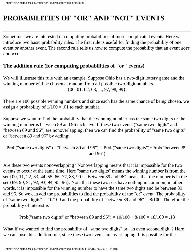
Sometimes we are interested in computing probabilities of more complicated events. Here we introduce two basic probability rules. The first rule is useful for finding the probability of one event or another event. The second rule tells us how to compute the probability that an event does not occur.
The addition rule (for computing probabilities of "or" events)
We will illustrate this rule with an example. Suppose Ohio has a two-digit lottery game and the winning number will be chosen at random from all possible two-digit numbers
{00, 01, 02, 03, ..., 97, 98, 99}.
There are 100 possible winning numbers and since each has the same chance of being chosen, we assign a probability of 1/100 = .01 to each number.
Suppose we want to find the probability that the winning number has the same two digits or the winning number is between 89 and 96 inclusive. If these two events ("same two digits" and "between 89 and 96") are nonoverlapping, then we can find the probability of "same two digits" or "between 89 and 96" by adding:
Prob("same two digits" or "between 89 and 96") = Prob("same two digits")+Prob("between 89 and 96")
Are these two events nonoverlapping? Nonoverlapping means that it is impossible for the two events to occur at the same time. Here "same two digits" means the winning number is from the set {00, 11, 22, 33, 44, 55, 66, 77, 88, 99}. "Between 89 and 96" means that the number is in the set {89, 90, 91, 92, 93, 94, 95, 96}. Note that these two sets have nothing in common; in other words, it is impossible for the winning number to have the same two digits and be between 89 and 96. So we can add the probabilities to find the probability of the "or" event. The probability of "same two digits" is 10/100 and the probability of "between 89 and 96" is 8/100. Therefore the probability of interest is
Prob("same two digits" or "between 89 and 96") = 10/100 + 8/100 = 18/100 = .18
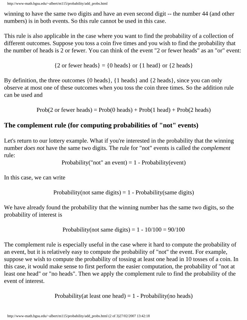
What if we wanted to find the probability of "same two digits" or "an even second digit"? Here we can't use this addition rule, since these two events are overlapping. It is possible for the
http://www-math.bgsu.edu/~albert/m115/probability/add_probs.html (1 of 3)27/02/2007 13:42:18
http://www-math.bgsu.edu/~albert/m115/probability/add_probs.html
winning to have the same two digits and have an even second digit -- the number 44 (and other numbers) is in both events. So this rule cannot be used in this case.
This rule is also applicable in the case where you want to find the probability of a collection of different outcomes. Suppose you toss a coin five times and you wish to find the probability that the number of heads is 2 or fewer. You can think of the event "2 or fewer heads" as an "or" event:
{2 or fewer heads} = {0 heads} or {1 head} or {2 heads}
By definition, the three outcomes {0 heads}, {1 heads} and {2 heads}, since you can only observe at most one of these outcomes when you toss the coin three times. So the addition rule can be used and
Prob(2 or fewer heads) = Prob(0 heads) + Prob(1 head) + Prob(2 heads)
The complement rule (for computing probabilities of "not" events)
Let's return to our lottery example. What if you're interested in the probability that the winning number does not have the same two digits. The rule for "not" events is called the complement rule:
Probability("not" an event) = 1 - Probability(event)
In this case, we can write
Probability(not same digits) = 1 - Probability(same digits)
We have already found the probability that the winning number has the same two digits, so the probability of interest is
Probability(not same digits) = 1 - 10/100 = 90/100
The complement rule is especially useful in the case where it hard to compute the probability of an event, but it is relatively easy to compute the probability of "not" the event. For example, suppose we wish to compute the probability of tossing at least one head in 10 tosses of a coin. In this case, it would make sense to first perform the easier computation, the probability of "not at least one head" or "no heads". Then we apply the complement rule to find the probability of the event of interest.
Probability(at least one head) = 1 - Probability(no heads)
http://www-math.bgsu.edu/~albert/m115/probability/add_probs.html (2 of 3)27/02/2007 13:42:18

http://www-math.bgsu.edu/~albert/m115/probability/add_probs.html
Return to AN INTRODUCTION TO PROBABILITY
Page Author: Jim Albert (© 2005) [email protected] Document: http://www-math.bgsu.edu/~albert/m115/probability/add_probs.html Last Modified: February 18, 2005
http://www-math.bgsu.edu/~albert/m115/probability/add_probs.html (3 of 3)27/02/2007 13:42:18
http://www-math.bgsu.edu/~albert/m115/probability/average_value.html
AN AVERAGE VALUE FOR A PROBABILITY DISTRIBUTION
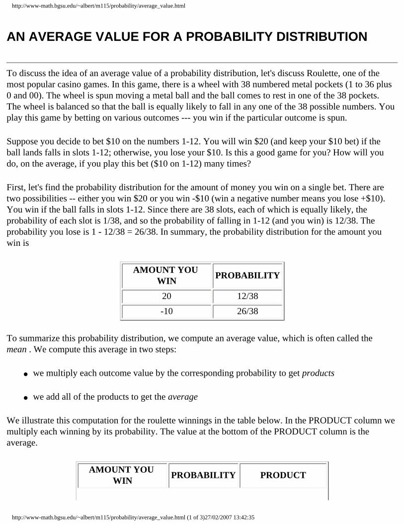
To discuss the idea of an average value of a probability distribution, let's discuss Roulette, one of the most popular casino games. In this game, there is a wheel with 38 numbered metal pockets (1 to 36 plus 0 and 00). The wheel is spun moving a metal ball and the ball comes to rest in one of the 38 pockets. The wheel is balanced so that the ball is equally likely to fall in any one of the 38 possible numbers. You play this game by betting on various outcomes --- you win if the particular outcome is spun.
Suppose you decide to bet $10 on the numbers 1-12. You will win $20 (and keep your $10 bet) if the ball lands falls in slots 1-12; otherwise, you lose your $10. Is this a good game for you? How will you do, on the average, if you play this bet ($10 on 1-12) many times?
First, let's find the probability distribution for the amount of money you win on a single bet. There are two possibilities -- either you win $20 or you win -$10 (win a negative number means you lose +$10). You win if the ball falls in slots 1-12. Since there are 38 slots, each of which is equally likely, the probability of each slot is 1/38, and so the probability of falling in 1-12 (and you win) is 12/38. The probability you lose is 1 - 12/38 = 26/38. In summary, the probability distribution for the amount you win is
AMOUNT YOU WIN
PROBABILITY
20 12/38
-10 26/38
To summarize this probability distribution, we compute an average value, which is often called the mean . We compute this average in two steps:
● we multiply each outcome value by the corresponding probability to get products
● we add all of the products to get the average
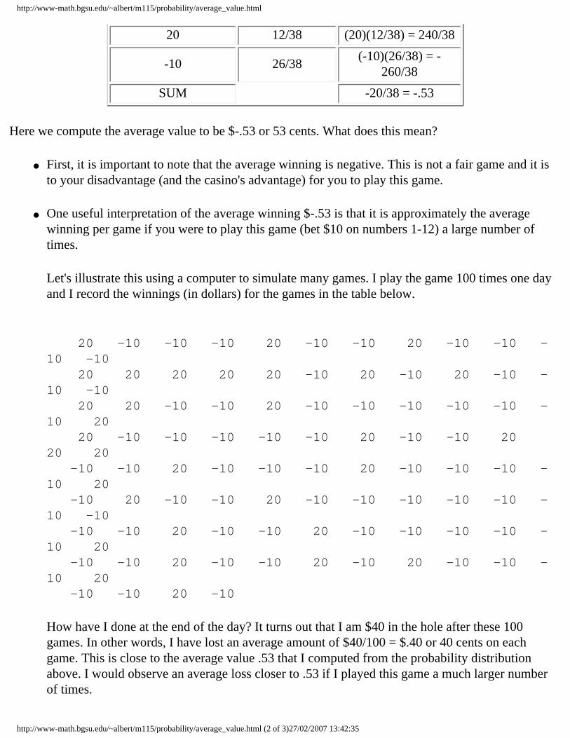
We illustrate this computation for the roulette winnings in the table below. In the PRODUCT column we multiply each winning by its probability. The value at the bottom of the PRODUCT column is the average.
AMOUNT YOU WIN
PROBABILITY PRODUCT
http://www-math.bgsu.edu/~albert/m115/probability/average_value.html (1 of 3)27/02/2007 13:42:35
http://www-math.bgsu.edu/~albert/m115/probability/average_value.html
20 12/38 (20)(12/38) = 240/38
-10 26/38 (-10)(26/38) = -
260/38
SUM -20/38 = -.53
Here we compute the average value to be $-.53 or 53 cents. What does this mean?
● First, it is important to note that the average winning is negative. This is not a fair game and it is to your disadvantage (and the casino's advantage) for you to play this game.
● One useful interpretation of the average winning $-.53 is that it is approximately the average winning per game if you were to play this game (bet $10 on numbers 1-12) a large number of times.
Let's illustrate this using a computer to simulate many games. I play the game 100 times one day and I record the winnings (in dollars) for the games in the table below.
20 -10 -10 -10 20 -10 -10 20 -10 -10 -10 -10 20 20 20 20 20 -10 20 -10 20 -10 -10 -10 20 20 -10 -10 20 -10 -10 -10 -10 -10 -10 20 20 -10 -10 -10 -10 -10 20 -10 -10 20 20 20 -10 -10 20 -10 -10 -10 20 -10 -10 -10 -10 20 -10 20 -10 -10 20 -10 -10 -10 -10 -10 -10 -10 -10 -10 20 -10 -10 20 -10 -10 -10 -10 -10 20 -10 -10 20 -10 -10 20 -10 20 -10 -10 -10 20 -10 -10 20 -10
How have I done at the end of the day? It turns out that I am $40 in the hole after these 100 games. In other words, I have lost an average amount of $40/100 = $.40 or 40 cents on each game. This is close to the average value .53 that I computed from the probability distribution above. I would observe an average loss closer to .53 if I played this game a much larger number of times.
http://www-math.bgsu.edu/~albert/m115/probability/average_value.html (2 of 3)27/02/2007 13:42:35
http://www-math.bgsu.edu/~albert/m115/probability/average_value.html
Return to AN INTRODUCTION TO PROBABILITY
Page Author: Jim Albert (© 1996) [email protected] Document: http://www-math.bgsu.edu/~albert/m115/probability/average_value.html Last Modified: November 24, 1996
http://www-math.bgsu.edu/~albert/m115/probability/average_value.html (3 of 3)27/02/2007 13:42:35
http://www-math.bgsu.edu/~albert/m115/probability/two_way_prob.html
UNDERSTANDING A TWO-WAY TABLE OF PROBABILITIES
Suppose we have a random process where an outcome is observed and two things are measured. For example, suppose we toss a fair coin three times and we observe the sequence
H T H
where H is a head and T a tail. Suppose we record
● the number of heads ● the number of runs in the sequence
In the three tosses above, we observe 2 heads and 3 runs in the sequence.
We are interested in talking about probabilities involving both measurements "number of heads" and "number of runs". These are described as joint probabilities , since they reflect the outcomes of two variables.
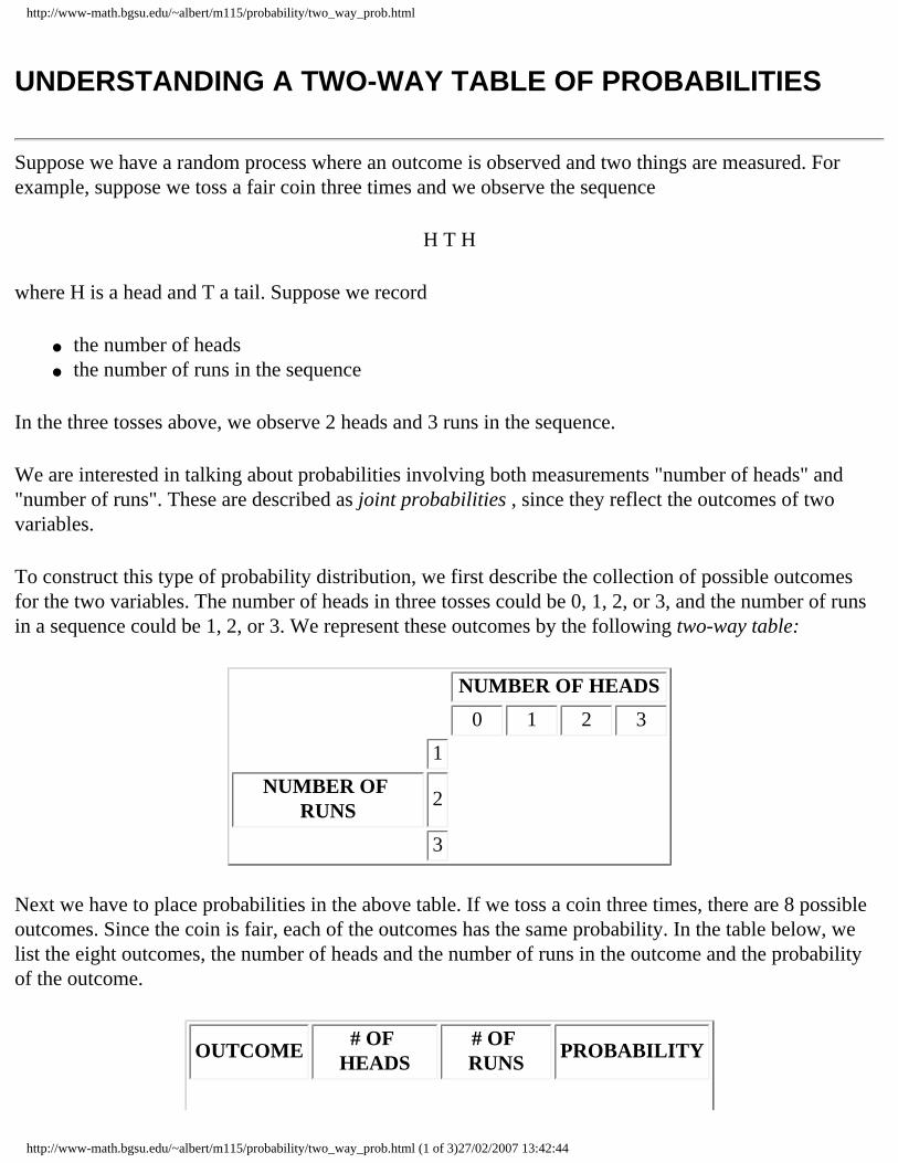
To construct this type of probability distribution, we first describe the collection of possible outcomes for the two variables. The number of heads in three tosses could be 0, 1, 2, or 3, and the number of runs in a sequence could be 1, 2, or 3. We represent these outcomes by the following two-way table:
NUMBER OF HEADS
0 1 2 3
1
NUMBER OF RUNS
2
3
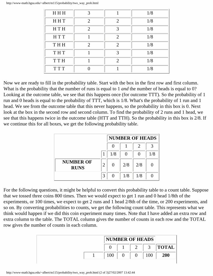
Next we have to place probabilities in the above table. If we toss a coin three times, there are 8 possible outcomes. Since the coin is fair, each of the outcomes has the same probability. In the table below, we list the eight outcomes, the number of heads and the number of runs in the outcome and the probability of the outcome.
OUTCOME # OF
HEADS # OF RUNS
PROBABILITY
http://www-math.bgsu.edu/~albert/m115/probability/two_way_prob.html (1 of 3)27/02/2007 13:42:44
http://www-math.bgsu.edu/~albert/m115/probability/two_way_prob.html
H H H 3 1 1/8
H H T 2 2 1/8
H T H 2 3 1/8
H T T 1 2 1/8
T H H 2 2 1/8
T H T 1 3 1/8
T T H 1 2 1/8
T T T 0 1 1/8
Now we are ready to fill in the probability table. Start with the box in the first row and first column. What is the probability that the number of runs is equal to 1 and the number of heads is equal to 0? Looking at the outcome table, we see that this happens once (for outcome TTT). So the probability of 1 run and 0 heads is equal to the probability of TTT, which is 1/8. What's the probability of 1 run and 1 head. We see from the outcome table that this never happens, so the probability in this box is 0. Next look at the box in the second row and second column. To find the probability of 2 runs and 1 head, we see that this happens twice in the outcome table (HTT and TTH). So the probability in this box is 2/8. If we continue this for all boxes, we get the following probability table.
NUMBER OF HEADS
0 1 2 3
1 1/8 0 0 1/8
NUMBER OF RUNS
2 0 2/8 2/8 0
3 0 1/8 1/8 0
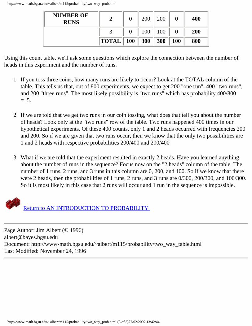
For the following questions, it might be helpful to convert this probability table to a count table. Suppose that we tossed three coins 800 times. Then we would expect to get 1 run and 0 head 1/8th of the experiments, or 100 times, we expect to get 2 runs and 1 head 2/8th of the time, or 200 experiments, and so on. By converting probabilities to counts, we get the following count table. This represents what we think would happen if we did this coin experiment many times. Note that I have added an extra row and extra column to the table. The TOTAL column gives the number of counts in each row and the TOTAL row gives the number of counts in each column.
NUMBER OF HEADS
0 1 2 3 TOTAL
1 100 0 0 100 200
http://www-math.bgsu.edu/~albert/m115/probability/two_way_prob.html (2 of 3)27/02/2007 13:42:44
http://www-math.bgsu.edu/~albert/m115/probability/two_way_prob.html
NUMBER OF RUNS
2 0 200 200 0 400
3 0 100 100 0 200
TOTAL 100 300 300 100 800
Using this count table, we'll ask some questions which explore the connection between the number of heads in this experiment and the number of runs.
1. If you toss three coins, how many runs are likely to occur? Look at the TOTAL column of the table. This tells us that, out of 800 experiments, we expect to get 200 "one run", 400 "two runs", and 200 "three runs". The most likely possibility is "two runs" which has probability 400/800 = .5.
2. If we are told that we get two runs in our coin tossing, what does that tell you about the number of heads? Look only at the "two runs" row of the table. Two runs happened 400 times in our hypothetical experiments. Of these 400 counts, only 1 and 2 heads occurred with frequencies 200 and 200. So if we are given that two runs occur, then we know that the only two possibilities are 1 and 2 heads with respective probabilities 200/400 and 200/400
3. What if we are told that the experiment resulted in exactly 2 heads. Have you learned anything about the number of runs in the sequence? Focus now on the "2 heads" column of the table. The number of 1 runs, 2 runs, and 3 runs in this column are 0, 200, and 100. So if we know that there were 2 heads, then the probabilities of 1 runs, 2 runs, and 3 runs are 0/300, 200/300, and 100/300. So it is most likely in this case that 2 runs will occur and 1 run in the sequence is impossible.
Return to AN INTRODUCTION TO PROBABILITY
Page Author: Jim Albert (© 1996) [email protected] Document: http://www-math.bgsu.edu/~albert/m115/probability/two_way_table.html Last Modified: November 24, 1996
http://www-math.bgsu.edu/~albert/m115/probability/two_way_prob.html (3 of 3)27/02/2007 13:42:44
http://www-math.bgsu.edu/~albert/m115/probability/list_activities.html
PROBABILITY ACTIVITIES
● Some questions about probability
● Is it a boy or a girl? CONCEPT: relative frequency view of probability
● What's Roberto Alomar's batting average? CONCEPT: relative frequency view of probability
● Probability phrases CONCEPT: subjective view of probability
● When was John Tyler born? CONCEPT: subjective view of probability
● How large is Pennsylvania? CONCEPT: subjective view of probability
● Assigning numbers to words CONCEPT: subjective view of probability
● Using chip-in-bowl experiments to help measure probabilities CONCEPTS: subjective view of probability , calibration experiment
● Who's going to be the 1997 NBA champion? CONCEPT: odds
● Tossing coins 1000 COIN TOSSES
http://www-math.bgsu.edu/~albert/m115/probability/list_activities.html (1 of 2)27/02/2007 13:42:53
http://www-math.bgsu.edu/~albert/m115/probability/list_activities.html
CONCEPT: constructing a probability table by simulation
● Ratings of Disney movies CONCEPTS: average value of a probability distribution , graphing probabilities
● The Minnesota cash lotto game CONCEPTS: odds , average value of a probability distribution
● Mothers and babies CONCEPTS: constructing a probability table by simulation , equally likely outcomes , listing all possible outcomes , Constructing a probability table by listing outcomes
● The collector's problem CONCEPTS: constructing a probability table by simulation , average value of a probability distribution
● Birthmonths CONCEPT: constructing a probability table by simulation
● Playoffs CONCEPT: constructing a probability table by simulation
● Rolling dice CONCEPTS: two-way table of probabilities , graphing probabilities
● Voting behavior in the Presidential Election CONCEPTS: two-way table of probabilities , graphing probabilities
● Playing yahtzee CONCEPT: two-way table of probabilities
AN INTRODUCTION TO PROBABILITY
Page Author: Jim Albert (© 1996) [email protected] Document: http://www-math.bgsu.edu/~albert/m115/probability/list_activities.html Last Modified: November 24, 1996
http://www-math.bgsu.edu/~albert/m115/probability/list_activities.html (2 of 2)27/02/2007 13:42:53