b747 cnb locus - cornell university · pdf filetion to the equations of motion for a flight...
TRANSCRIPT
Chapter 5
Dynamic Stability
These notes provide a brief background for the response of linear systems, with applica-tion to the equations of motion for a flight vehicle. The description is meant to providethe basic background in linear algebra for understanding modern tools for analyzing theresponse of linear systems, and provide examples of their application to flight vehicledynamics. Examples for both longitudinal and lateral/directional motions are provided,and simple, lower-order approximations to the various modes are used to elucidate theroles of relevant aerodynamic properties of the vehicle.
5.1 Mathematical Background
5.1.1 An Introductory Example
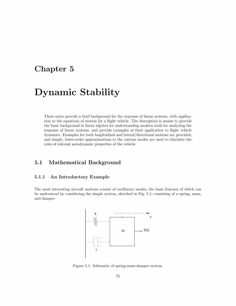
The most interesting aircraft motions consist of oscillatory modes, the basic features of which canbe understood by considering the simple system, sketched in Fig. 5.1, consisting of a spring, mass,and damper.
m F(t)
k
c
x
Figure 5.1: Schematic of spring-mass-damper system.
75

76 CHAPTER 5. DYNAMIC STABILITY
The dynamics of this system are described by the second-order ordinary differential equation
md2x
dt2+ c
dx
dt+ kx = F (t) (5.1)
where m is the mass of the system, c is the damping parameter, and k is the spring constant ofthe restoring force. We generally are interested in both the free response of the system to an initialperturbation (with F (t) = 0), and the forced response to time-varying F (t). The free response isrelevant to the question of stability – i.e., the response to an infinitesimal perturbation from anequilibrium state of the system, while the forced response is relevant to control response.
The free response is the solution to the homogeneous equation, which can be written
d2x
dt2+( c
m
) dx
dt+
(
k
m
)
x = 0 (5.2)
Solutions of this equation are generally of the form
x = Aeλt (5.3)
where A is a constant determined by the initial perturbation. Substitution of Eq. (5.3) into thedifferential equation yields the characteristic equation
λ2 +( c
m
)
λ+
(
k
m
)
= 0 (5.4)
which has roots
λ = − c
2m±√
( c
2m
)2
−(
k
m
)
(5.5)
The nature of the response depends on whether the second term in the above expression is real orimaginary, and therefore depends on the relative magnitudes of the damping parameter c and thespring constant k. We can re-write the characteristic equation in terms of a variable defined by theratio of the two terms in the square root
(
c2m
)2
(
km
) =c2
4mk≡ ζ2 (5.6)
and a variable explicitly depending on the spring constant k, which we will choose (for reasons thatwill become obvious later) to be
k
m≡ ω2
n (5.7)
In terms of these new variables, the original Eq. (5.2) can be written as
d2x
dt2+ 2ζωn
dx
dt+ ω2
nx = 0 (5.8)
The corresponding characteristic equation takes the form
λ2 + 2ζωnλ+ ω2n = 0 (5.9)
and its roots can now be written in the suggestive forms
λ =
−ζωn ± ωn
√
ζ2 − 1 for ζ > 1
−ζωn for ζ = 1
−ζωn ± iωn
√
1 − ζ2 for ζ < 1
(5.10)
5.1. MATHEMATICAL BACKGROUND 77
Overdamped System
For cases in which ζ > 1, the characteristic equation has two (distinct) real roots, and the solutiontakes the form
x = a1eλ1t + a2e
λ2t (5.11)
where
λ1 = −ωn
(
ζ +√
ζ2 − 1)
λ2 = −ωn
(
ζ −√
ζ2 − 1) (5.12)
The constants a1 and a2 are determined from the initial conditions
x(0) = a1 + a2
x(0) = a1λ1 + a2λ2
(5.13)
or, in matrix form,(
1 1λ1 λ2
)(
a1
a2
)
=
(
x(0)x(0)
)
(5.14)
Since the determinant of the coefficient matrix in these equations is equal to λ2 −λ1, the coefficientmatrix is non-singular so long as the characteristic values λ1 and λ2 are distinct – which is guaranteedby Eqs. (5.12) when ζ > 1. Thus, for the overdamped system (ζ > 1), the solution is completelydetermined by the initial values of x and x, and consists of a linear combination of two decayingexponentials.
The reciprocal of the undamped natural frequency ωn forms a natural time scale for this problem,so if we introduce the dimensionless time
t = ωnt (5.15)
then Eq. (5.8) can be written
d2x
dt2+ 2ζ
dx
dt+ x = 0 (5.16)
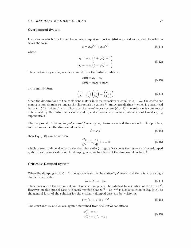
which is seen to depend only on the damping ratio ζ. Figure 5.2 shows the response of overdampedsystems for various values of the damping ratio as functions of the dimensionless time t.
Critically Damped System
When the damping ratio ζ = 1, the system is said to be critically damped , and there is only a singlecharacteristic value
λ1 = λ2 = −ωn (5.17)
Thus, only one of the two initial conditions can, in general, be satisfied by a solution of the form eλt.However, in this special case it is easily verified that teλt = te−ωnt is also a solution of Eq. (5.8), sothe general form of the solution for the critically damped case can be written as
x = (a1 + a2t) e−ωnt (5.18)
The constants a1 and a2 are again determined from the initial conditions
x(0) = a1
x(0) = a1λ1 + a2
(5.19)
78 CHAPTER 5. DYNAMIC STABILITY
0 2 4 6 8 10 12 14 16 18 20−0.2
0
0.2
0.4
0.6
0.8
1
Normalized time, ωn t
Dis
plac
emen
t, x
ζ = 1
ζ = 2
ζ = 5
ζ = 10
0 2 4 6 8 10 12 14 16 18 20−0.1
0
0.1
0.2
0.3
0.4
Normalized time, ωn t
Dis
plac
emen
t, x
ζ = 1
ζ = 2
ζ = 5
ζ = 10
(a) x(0) = 1.0 (b) x(0) = 1.0
Figure 5.2: Overdamped response of spring-mass-damper system. (a) Displacement perturbation:x(0) = 1.0; x(0) = 0. (b) Velocity perturbation: x(0) = 1.0; x(0) = 0.
or, in matrix form,(
1 0λ1 1
)(
a1
a2
)
=
(
x(0)x(0)
)
(5.20)
Since the determinant of the coefficient matrix in these equations is always equal to unity, thecoefficient matrix is non-singular. Thus, for the critically damped system (ζ = 1), the solution isagain completely determined by the initial values of x and x, and consists of a linear combinationof a decaying exponential and a term proportional to te−ωnt. For any positive value of ωn theexponential decays more rapidly than any positive power of t, so the solution again decays, nearly
exponentially.
Figures 5.2 and 5.3 include the limiting case of critically damped response for Eq. (5.16).
Underdamped System
When the damping ratio ζ < 1, the system is said to be underdamped , and the roots of the charac-teristic equation consist of the complex conjugate pair
λ1 = ωn
(
−ζ + i√
1 − ζ2)
λ2 = ωn
(
−ζ − i√
1 − ζ2) (5.21)
Thus, the general form of the solution can be written
x = e−ζωnt[
a1 cos(
ωn
√
1 − ζ2t)
+ a2 sin(
ωn
√
1 − ζ2t)]
(5.22)
The constants a1 and a2 are again determined from the initial conditions
x(0) = a1
x(0) = −ζωna1 + ωn
√
1 − ζ2a2
(5.23)
or, in matrix form,(
1 0
−ζωn ωn
√
1 − ζ2
)(
a1
a2
)
=
(
x(0)x(0)
)
(5.24)

5.1. MATHEMATICAL BACKGROUND 79
0 2 4 6 8 10 12 14 16 18 20−1
−0.8
−0.6
−0.4
−0.2
0
0.2
0.4
0.6
0.8
1
Normalized time, ωn t
Dis
plac
emen
t, x
ζ = 0.1
ζ = 0.3
ζ = 0.6
ζ = 1
0 2 4 6 8 10 12 14 16 18 20−1
−0.8
−0.6
−0.4
−0.2
0
0.2
0.4
0.6
0.8
1
Normalized time, ωn t
Dis
plac
emen
t, x
ζ = 0.1
ζ = 0.3
ζ = 0.6
ζ = 1
(a) x(0) = 1.0 (b) x(0) = 1.0
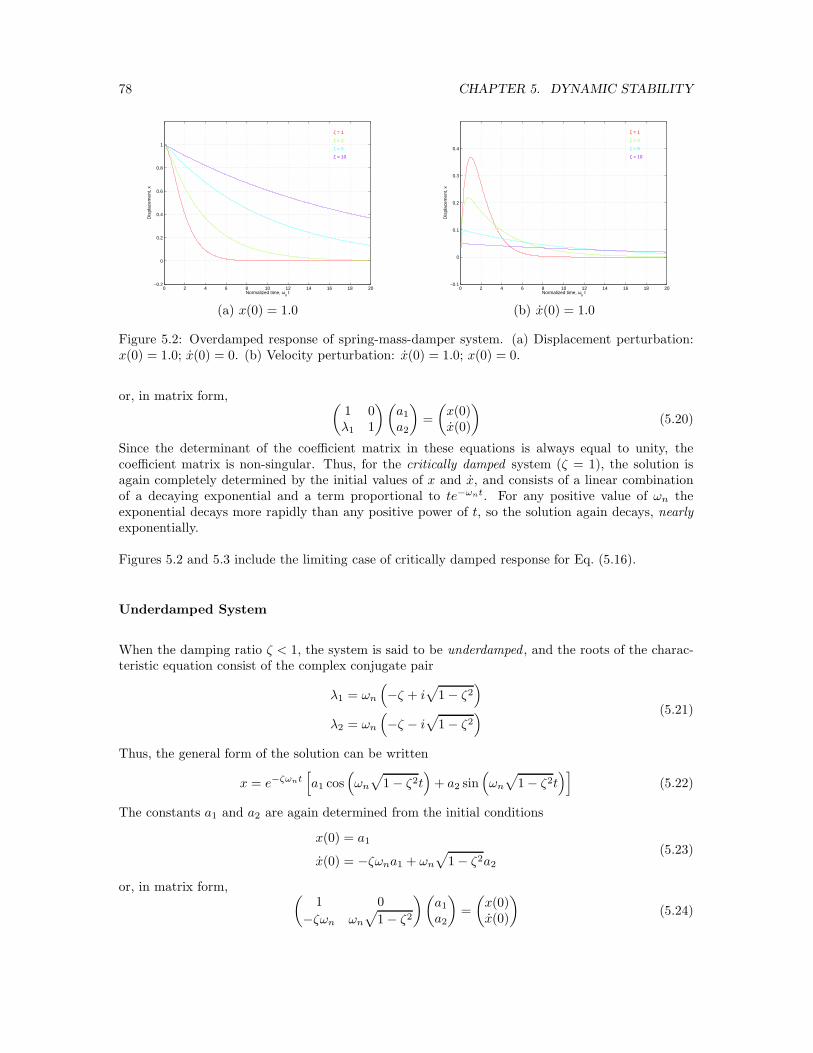
Figure 5.3: Underdamped response of spring-mass-damper system. (a) Displacement perturbation:x(0) = 1.0; x(0) = 0. (b) Velocity perturbation: x(0) = 1.0; x(0) = 0.
Since the determinant of the coefficient matrix in these equations is equal to ωn
√
1 − ζ2, the systemis non-singular when ζ < 1, and the solution is completely determined by the initial values of x andx. Figure 5.3 shows the response of the underdamped system Eq. (5.16) for various values of thedamping ratio, again as a function of the dimensionless time t.
As is seen from Eq. (5.22), the solution consists of an exponentially decaying sinusoidal motion.This motion is characterized by its period and the rate at which the oscillations are damped. Theperiod is given by
T =2π
ωn
√
1 − ζ2(5.25)
and the time to damp to 1/n times the initial amplitude is given by1
t1/n =lnn
ωnζ(5.26)
For these oscillatory motions, the damping frequently is characterized by the number of cycles todamp to 1/n times the initial amplitude, which is given by
N1/n =t1/n
T=
lnn
2π
√
1 − ζ2
ζ(5.27)
Note that this latter quantity is independent of the undamped natural frequency; i.e., it dependsonly on the damping ratio ζ.
5.1.2 Systems of First-order Equations
Although the equation describing the spring-mass-damper system of the previous section was solvedin its original form, as a single second-order ordinary differential equation, it is useful for later
1The most commonly used values of n are 2 and 10, corresponding to the times to damp to 1/2 the initial amplitudeand 1/10 the initial amplitude, respectively.

80 CHAPTER 5. DYNAMIC STABILITY
generalization to re-write it as a system of coupled first-order differential equations by defining
x1 = x
x2 =dx
dt
(5.28)
Equation (5.8) can then be written as
d
dt
(
x1
x2
)
=
(
0 1−ω2
n −2ζωn
)(
x1
x2
)
+
(
01m
)
F (t) (5.29)
which has the general formx = Ax + Bη (5.30)
where x = (x1, x2)T , the dot represents a time derivative, and η(t) = F (t) will be identified as the
control input.
The free response is then governed by the system of equations
x = Ax (5.31)
and substitution of the general formx = xie
λit (5.32)
into Eqs. (5.31) requires(A − λiI)xi = 0 (5.33)
Thus, the free response of the system in seen to be completely determined by the eigenstructure (i.e.,the eigenvalues and eigenvectors) of the plant matrix A. The vector xi is seen to be the eigenvectorassociated with the eigenvalue λi of the matrix A and, when the eigenvalues are unique, the generalsolution can be expressed as a linear combination of the form
x =
2∑
i=1
aixieλit (5.34)
where the constants ai are determined by the initial conditions. The modal matrix Q of A is definedas the matrix whose columns are the eigenvectors of A
Q =(
x1 x2
)
(5.35)
so the initial values of the vector x are given by
x(0) =
2∑
i=1
aixi = Qa (5.36)
where the elements of the vectora = {a1, a2}T
correspond to the coefficients in the modal expansion of the solution in the form of Eq. (5.34). Whenthe eigenvalues are complex, they must appear in complex conjugate pairs, and the correspondingeigenvectors also are complex conjugates, so the solution corresponding to a complex conjugate pairof eigenvalues again corresponds to an exponentially damped harmonic oscillation.
While the above analysis corresponds to the second-order system treated previously, the advantage ofviewing is as a system of first-order equations is that, once we have shifted our viewpoint the analysis
5.2. LONGITUDINAL MOTIONS 81
carries through for a system of any order. In particular, the simplest complete linear analyses of eitherlongitudinal or lateral/directional dynamics will lead to fourth-order systems – i.e., to systems offour coupled first-order differential equations. In practice, most of the required operations involvingeigenvalues and eigenvectors can be accomplished easily using numerical software packages, such asMatlab
5.2 Longitudinal Motions
In this section, we develop the small-disturbance equations for longitudinal motions in standardstate-variable form. Recall that the linearized equations describing small longitudinal perturbationsfrom a longitudinal equilibrium state can be written
[
d
dt−Xu
]
u+ g0 cosΘ0θ −Xww = Xδeδe +XδT
δT
−Zuu+
[
(1 − Zw)d
dt− Zw
]
w − [u0 + Zq] q + g0 sin Θ0θ = Zδeδe + ZδT
δT
−Muu−[
Mwd
dt+Mw
]
w +
[
d
dt−Mq
]
q = Mδeδe +MδT
δT
(5.37)
If we introduce the longitudinal state variable vector
x = [u w q θ]T
(5.38)
and the longitudinal control vectorη = [δe δT ]T (5.39)
these equations are equivalent to the system of first-order equations
Inx = Anx + Bnη (5.40)
where x represents the time derivative of the state vector x, and the matrices appearing in thisequation are
An =
Xu Xw 0 −g0 cosΘ0
Zu Zw u0 + Zq −g0 sin Θ0
Mu Mw Mq 00 0 1 0
In =
1 0 0 00 1 − Zw 0 00 −Mw 1 00 0 0 1
, Bn =
XδeXδT
ZδeZδT
MδeMδT
0 0
(5.41)
It is not difficult to show that the inverse of In is
I−1n =
1 0 0 00 1
1−Zw0 0
0 Mw
1−Zw1 0
0 0 0 1
(5.42)
so premultiplying Eq. (5.40) by I−1n gives the standard form
x = Ax + Bη (5.43)

82 CHAPTER 5. DYNAMIC STABILITY
where
A =
Xu Xw 0 −g0 cosΘ0Zu
1−Zw
Zw
1−Zw
u0+Zq
1−Zw
−g0 sin Θ0
1−Zw
Mu + MwZu
1−ZwMw + MwZw
1−ZwMq +
(u0+Zq)Mw
1−Zw
−Mwg0 sin Θ0
1−Zw
0 0 1 0
B =
XδeXδT
Zδe
1−Zw
ZδT
1−Zw
Mδe+
MwZδe
1−ZwMδT
+MwZδT
1−Zw
0 0
(5.44)
Note that
Zw =QSc
2mu20
CZα = − 1
2µCLα (5.45)
and
Zq =QSc
2mu0CZq = −u0
2µCLq (5.46)
Since the aircraft mass parameter µ is typically large (on the order of 100), it is common to neglectZw with respect to unity and to neglect Zq relative to u0, in which case the matrices A and B canbe approximated as
A =
Xu Xw 0 −g0 cosΘ0
Zu Zw u0 −g0 sin Θ0
Mu +MwZu Mw +MwZw Mq + u0Mw −Mwg0 sin Θ0
0 0 1 0
B =
XδeXδT
ZδeZδT
Mδe+MwZδe
MδT+MwZδT
0 0
(5.47)
This is the approximate form of the linearized equations for longitudinal motions as they appear inmany texts (see, e.g., Eqs. (4.53) and (4.54) in [3]2).
The various dimensional stability derivatives appearing in Eqs. (5.44) and (5.47) are related to theirdimensionless aerodynamic coefficient counterparts in Table 5.1; these data were also presented inTable 4.1 in the previous chapter.
5.2.1 Modes of Typical Aircraft
The natural response of most aircraft to longitudinal perturbations typically consists of two under-damped oscillatory modes having rather different time scales. One of the modes has a relativelyshort period and is usually quite heavily damped; this is called the short period mode. The othermode has a much longer period and is rather lightly damped; this is called the phugoid mode.
We illustrate this response using the stability derivatives for the Boeing 747 aircraft at its Mach 0.25power approach configuration at standard sea-level conditions. The aircraft properties and flight
2The equations in [3] also assume level flight, or Θ0 = 0.
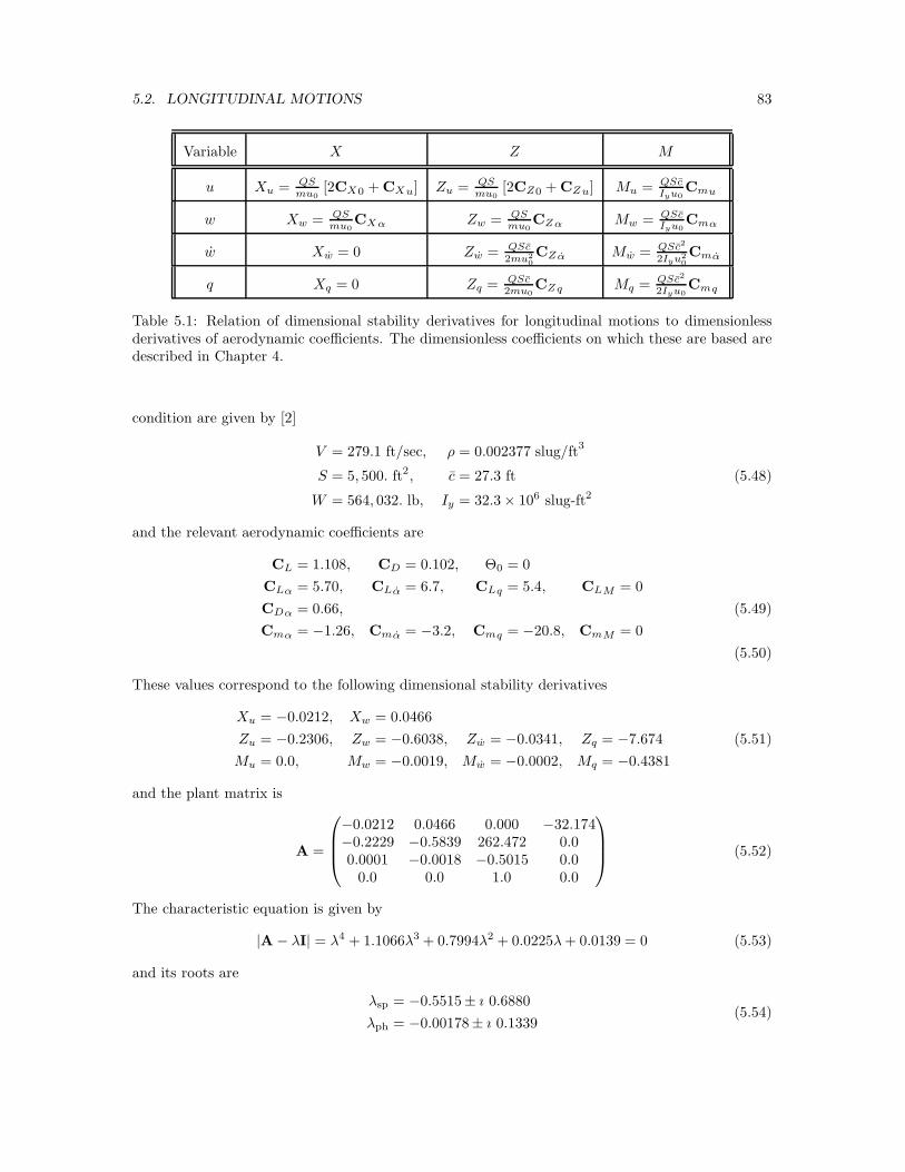
5.2. LONGITUDINAL MOTIONS 83
Variable X Z M
u Xu = QSmu0
[2CX0 + CXu] Zu = QSmu0
[2CZ0 + CZu] Mu = QScIyu0
Cmu
w Xw = QSmu0
CXα Zw = QSmu0
CZα Mw = QScIyu0
Cmα
w Xw = 0 Zw = QSc2mu2
0
CZα Mw = QSc2
2Iyu20
Cmα
q Xq = 0 Zq = QSc2mu0
CZq Mq = QSc2
2Iyu0Cmq
Table 5.1: Relation of dimensional stability derivatives for longitudinal motions to dimensionlessderivatives of aerodynamic coefficients. The dimensionless coefficients on which these are based aredescribed in Chapter 4.
condition are given by [2]
V = 279.1 ft/sec, ρ = 0.002377 slug/ft3
S = 5, 500. ft2, c = 27.3 ft (5.48)
W = 564, 032. lb, Iy = 32.3 × 10⁶ slug-ft2
and the relevant aerodynamic coefficients are
CL = 1.108, CD = 0.102, Θ0 = 0
CLα = 5.70, CLα = 6.7, CLq = 5.4, CLM = 0
CDα = 0.66, (5.49)
Cmα = −1.26, Cmα = −3.2, Cmq = −20.8, CmM = 0
(5.50)
These values correspond to the following dimensional stability derivatives
Xu = −0.0212, Xw = 0.0466
Zu = −0.2306, Zw = −0.6038, Zw = −0.0341, Zq = −7.674 (5.51)
Mu = 0.0, Mw = −0.0019, Mw = −0.0002, Mq = −0.4381
and the plant matrix is
A =
−0.0212 0.0466 0.000 −32.174−0.2229 −0.5839 262.472 0.00.0001 −0.0018 −0.5015 0.0
0.0 0.0 1.0 0.0
(5.52)
The characteristic equation is given by
|A − λI| = λ4 + 1.1066λ3 + 0.7994λ2 + 0.0225λ+ 0.0139 = 0 (5.53)
and its roots are
λsp = −0.5515± ı 0.6880
λph = −0.00178± ı 0.1339(5.54)

84 CHAPTER 5. DYNAMIC STABILITY
0 1 2 3 4 5 6 7 8 9 10−2
−1.5
−1
−0.5
0
0.5
1
1.5
2
Time, sec
Sta
te V
aria
ble
Speed, u/u
0
Angle of attackPitch ratePitch angle
0 20 40 60 80 100 120 140 160 180 200
−1
−0.8
−0.6
−0.4
−0.2
0
0.2
0.4
0.6
0.8
1
Time, sec
Sta
te V
aria
ble
Speed, u/u
0
Angle of attackPitch ratePitch angle
(a) Short period (b) Phugoid
Figure 5.4: Response of Boeing 747 aircraft to longitudinal perturbations. (a) Short period response;(b) Phugoid response.
where, as suggested by the subscripts, the first pair of roots corresponds to the short period mode,and the second pair corresponds to the phugoid mode. The damping ratios of the two modes arethus given by
ζsp =
√
√
√
√
1
1 +(
ηξ
)2
sp
=
√
1
1 +(
0.68800.5515
)2 = 0.6255
ζph =
√
√
√
√
1
1 +(
ηξ
)2
ph
=
√
1
1 +(
0.13390.00178
)2 = 0.0133
(5.55)
where ξ and η are the real and imaginary parts of the respective roots, and the undamped naturalfrequencies of the two modes are
ωnsp=
−ξspζsp
=0.5515
0.6255= 0.882 sec−1
ωnph=
−ξph
ζph=
0.00178
0.0133= 0.134 sec−1
(5.56)
The periods of the two modes are given by
Tsp =2π
ωnsp
√
1 − ζ2sp
= 9.13 sec (5.57)
and
Tph =2π
ωnph
√
1 − ζ2ph
= 46.9 sec (5.58)
respectively.
Figure 5.4 illustrates the short period and phugoid responses for the Boeing 747 under these condi-tions. These show the time histories of the state variables following an initial perturbation that ischosen to excite only the (a) short period mode or the (b) phugoid mode, respectively.

5.2. LONGITUDINAL MOTIONS 85
It should be noted that the dimensionless velocity perturbations u/u0 and α = w/u0 are plottedin these figures, in order to allow comparisons with the other state variables. The plant matrixcan be modified to reflect this choice of state variables as follows. The elements of the first twocolumns of the original plant matrix should be multiplied by u0, then the entire plant matrix shouldbe premultiplied by the diagonal matrix having elements diag(1/u0, 1/u0, 1, 1). The combination ofthese two steps is equivalent to dividing the elements in the upper right two-by-two block of theplant matrix A by u0, and multiplying the elements in the lower left two-by-two block by u0. Theresulting scaled plant matrix is then given by
A =
−0.0212 0.0466 0.000 −0.1153−0.2229 −0.5839 0.9404 0.00.0150 −0.5031 −0.5015 0.0
0.0 0.0 1.0 0.0
(5.59)
Note that, after this re-scaling, the magnitudes of the elements in the upper-right and lower-left twoby two blocks of the plant matrix are more nearly the same order as the other terms (than theywere in the original form).
It is seen in the figures that the short period mode is, indeed, rather heavily damped, while thephugoid mode is very lightly damped. In spite of the light damping of the phugoid, it generally doesnot cause problems for the pilot because its time scale is long enough that minor control inputs cancompensate for the excitation of this mode by disturbances.
The relative magnitudes and phases of the perturbations in state variables for the two modes canbe seen from the phasor diagrams for the various modes. These are plots in the complex plane ofthe components of the mode eigenvector corresponding to each of the state variables. The phasorplots for the short period and phugoid modes for this example are shown in Fig. 5.5. It is seen thatthe airspeed variation in the short period mode is, indeed, negligibly small, and the pitch angle θlags the pitch rate q by substantially more than 90 degrees (due to the relatively large damping).The phugoid is seen to consist primarily of perturbations in airspeed and pitch angle. Although it isdifficult to see on the scale of Fig. 5.5 (b), the pitch angle θ lags the pitch rate q by almost exactly90 degrees for the phugoid (since the motion is so lightly damped it is nearly harmonic).
An arbitrary initial perturbation will generally excite both the short period and phugoid modes.This is illustrated in Fig. 5.6, which plots the time histories of the state variables following an initialperturbation in angle of attack. Figure 5.6 (a) shows the early stages of the response (on a time
Re
q
Im
w/u0
θ
q
w/u0 Re
Im
u/u0
θ
(a) Short period (b) Phugoid
Figure 5.5: Phasor diagrams for longitudinal modes of the Boeing 747 aircraft in powered approachat M = 0.25. Perturbation in normalized speed u/u0 is too small to be seen in short period mode.

86 CHAPTER 5. DYNAMIC STABILITY
0 1 2 3 4 5 6 7 8 9 10
−1.5
−1
−0.5
0
0.5
1
1.5
Time, sec
Sta
te V
aria
ble
Speed, u/u
0
Angle of attackPitch ratePitch angle
0 10 20 30 40 50 60 70 80 90 100
−1.5
−1
−0.5
0
0.5
1
1.5
Time, sec
Sta
te V
aria
ble
Speed, u/u
0
Angle of attackPitch ratePitch angle
(a) Short period (b) Phugoid
Figure 5.6: Response of Boeing 747 aircraft to unit perturbation in angle of attack. (a) Time scalechosen to emphasize short period response; (b) Time scale chosen to emphasize phugoid response.
scale appropriate for the short period mode), while Fig. 5.6 (b) shows the response on a time scaleappropriate for describing the phugoid mode.
The pitch- and angle-of-attack-damping are important for damping the short period mode, whileits frequency is determined primarily by the pitch stiffness. The period of the phugoid mode isnearly independent of vehicle parameters, and is very nearly inversely proportional to airspeed. Thedamping ratio for the phugoid is approximately proportional to the ratio CD/CL, which is smallfor efficient aircraft. These properties can be seen from the approximate analyses of the two modespresented in the following two sections.
5.2.2 Approximation to Short Period Mode
The short period mode typically occurs so quickly that it proceeds at essentially constant vehiclespeed. A useful approximation for the mode can thus be developed by setting u = 0 and solving
(1 − Zw) w = Zww + (u0 + Zq) q
−Mww + q = Mww +Mqq(5.60)
which can be written in state-space form as
d
dt
(
wq
)
=
(
Zw
1−Zw
u0+Zq
1−Zw
Mw + MwZw
1−ZwMq +Mw
u0+Zq
1−Zw
)
(
wq
)
(5.61)
SinceZq
u0=
QSc
2mu20
CZq = −ηVHat
µ(5.62)
where µ, the aircraft relative mass parameter, is usually large (on the order of one hundred), it isconsistent with the level of our approximation to neglect Zq relative to u0. Also, we note that
Zw =QSc
2mu20
CZα = −ηVHat
µ
dǫ
dα(5.63)
5.2. LONGITUDINAL MOTIONS 87
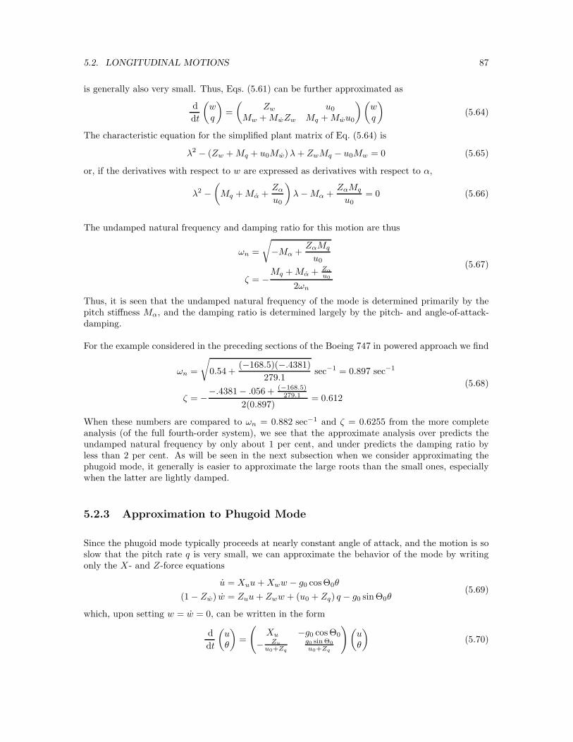
is generally also very small. Thus, Eqs. (5.61) can be further approximated as
d
dt
(
wq
)
=
(
Zw u0
Mw +MwZw Mq +Mwu0
)(
wq
)
(5.64)
The characteristic equation for the simplified plant matrix of Eq. (5.64) is
λ2 − (Zw +Mq + u0Mw)λ+ ZwMq − u0Mw = 0 (5.65)
or, if the derivatives with respect to w are expressed as derivatives with respect to α,
λ2 −(
Mq +Mα +Zα
u0
)
λ−Mα +ZαMq
u0= 0 (5.66)
The undamped natural frequency and damping ratio for this motion are thus
ωn =
√
−Mα +ZαMq
u0
ζ = −Mq +Mα + Zα
u0
2ωn
(5.67)
Thus, it is seen that the undamped natural frequency of the mode is determined primarily by thepitch stiffness Mα, and the damping ratio is determined largely by the pitch- and angle-of-attack-damping.
For the example considered in the preceding sections of the Boeing 747 in powered approach we find
ωn =
√
0.54 +(−168.5)(−.4381)
279.1sec−1 = 0.897 sec−1
ζ = −−.4381− .056 + (−168.5)279.1
2(0.897)= 0.612
(5.68)
When these numbers are compared to ωn = 0.882 sec−1 and ζ = 0.6255 from the more completeanalysis (of the full fourth-order system), we see that the approximate analysis over predicts theundamped natural frequency by only about 1 per cent, and under predicts the damping ratio byless than 2 per cent. As will be seen in the next subsection when we consider approximating thephugoid mode, it generally is easier to approximate the large roots than the small ones, especiallywhen the latter are lightly damped.
5.2.3 Approximation to Phugoid Mode
Since the phugoid mode typically proceeds at nearly constant angle of attack, and the motion is soslow that the pitch rate q is very small, we can approximate the behavior of the mode by writingonly the X- and Z-force equations
u = Xuu+Xww − g0 cosΘ0θ
(1 − Zw) w = Zuu+ Zww + (u0 + Zq) q − g0 sin Θ0θ(5.69)
which, upon setting w = w = 0, can be written in the form
d
dt
(
uθ
)
=
(
Xu −g0 cosΘ0
− Zu
u0+Zq
g0 sin Θ0
u0+Zq
)
(
uθ
)
(5.70)

88 CHAPTER 5. DYNAMIC STABILITY
Since, as has been seen in Eq. (5.62), Zq is typically very small relative to the speed u0, it is consistentwith our neglect of q and w also to neglect Zq relative to u0. Also, we will consider only the case oflevel flight for the initial equilibrium, so Θ0 = 0, and Eq. (5.70) becomes
d
dt
(
uθ
)
=
(
Xu −g0−Zu
u00
)(
uθ
)
(5.71)
The characteristic equation for the simplified plant matrix of Eq. (5.71) is
λ2 −Xuλ− g0u0Zu = 0 (5.72)
The undamped natural frequency and damping ratio for this motion are thus
ωn =
√
− g0u0Zu
ζ =−Xu
2ωn
(5.73)
It is useful to express these results in terms of dimensionless aerodynamic coefficients. Recall that
Zu = − QS
mu0[2CL0 + MCLM] (5.74)
and, for the case of a constant-thrust propulsive system,
Xu = − QS
mu0[2CD0 + MCDM] (5.75)
so, if we further neglect compressibility effects, we have
ωn =√
2g0u0
ζ =1√2
CD0
CL0
(5.76)
Thus, according to this approximation, the undamped natural frequency of the phugoid is a functiononly of the flight velocity, and the damping ratio is proportional to the drag-to-lift ratio. Since thelatter quantity is small for an efficient flight vehicle, this explains why the phugoid typically is verylightly damped.
For the example of the Boeing 747 in powered approach we find
ωn =√
232.174 ft/sec
2
279.1 ft/sec= 0.163 sec−1
ζ =1√2
0.102
1.108= 0.0651
(5.77)
When these numbers are compared to ωn = 0.134 sec−1 and ζ = 0.0133 from the more completeanalysis (of the full fourth-order system), we see that the approximate analysis over predicts theundamped natural frequency by about 20 per cent, and over predicts the damping ratio by a factor ofalmost 5. Nevertheless, this simplified analysis gives insight into the important parameters governingthe mode.
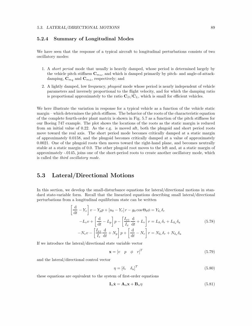
5.3. LATERAL/DIRECTIONAL MOTIONS 89
5.2.4 Summary of Longitudinal Modes
We have seen that the response of a typical aircraft to longitudinal perturbations consists of twooscillatory modes:
1. A short period mode that usually is heavily damped, whose period is determined largely bythe vehicle pitch stiffness Cmα, and which is damped primarily by pitch- and angle-of-attack-damping, Cmq and Cmα, respectively; and
2. A lightly damped, low frequency, phugoid mode whose period is nearly independent of vehicleparameters and inversely proportional to the flight velocity, and for which the damping ratiois proportional approximately to the ratio CD/CL, which is small for efficient vehicles.
We here illustrate the variation in response for a typical vehicle as a function of the vehicle staticmargin – which determines the pitch stiffness. The behavior of the roots of the characteristic equationof the complete fourth-order plant matrix is shown in Fig. 5.7 as a function of the pitch stiffness forour Boeing 747 example. The plot shows the locations of the roots as the static margin is reducedfrom an initial value of 0.22. As the c.g. is moved aft, both the phugoid and short period rootsmove toward the real axis. The short period mode becomes critically damped at a static marginof approximately 0.0158, and the phugoid becomes critically damped at a value of approximately0.0021. One of the phugoid roots then moves toward the right-hand plane, and becomes neutrallystable at a static margin of 0.0. The other phugoid root moves to the left and, at a static margin ofapproximately -.0145, joins one of the short-period roots to create another oscillatory mode, whichis called the third oscillatory mode.
5.3 Lateral/Directional Motions
In this section, we develop the small-disturbance equations for lateral/directional motions in stan-dard state-variable form. Recall that the linearized equations describing small lateral/directionalperturbations from a longitudinal equilibrium state can be written
[
d
dt− Yv
]
v − Ypp+ [u0 − Yr] r − g0 cosΘ0φ = Yδrδr
−Lvv +
[
d
dt− Lp
]
p−[
Ixz
Ix
d
dt+ Lr
]
r = Lδrδr + Lδa
δa
−Nvv −[
Ixz
Iz
d
dt+Np
]
p+
[
d
dt−Nr
]
r = Nδrδr +Nδa
δa
(5.78)
If we introduce the lateral/directional state variable vector
x = [v p φ r]T (5.79)
and the lateral/directional control vector
η = [δr δa]T
(5.80)
these equations are equivalent to the system of first-order equations
Inx = Anx + Bnη (5.81)
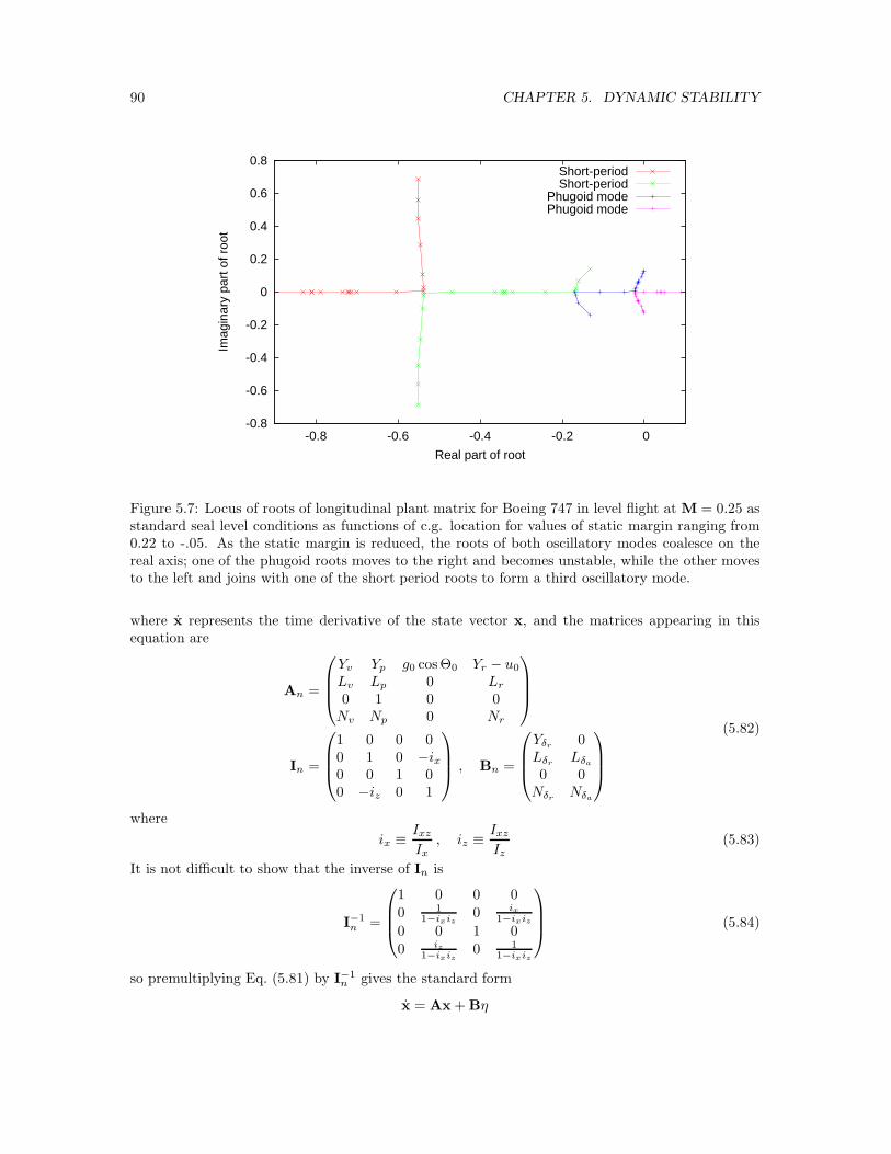
90 CHAPTER 5. DYNAMIC STABILITY
-0.8
-0.6
-0.4
-0.2
0
0.2
0.4
0.6
0.8
-0.8 -0.6 -0.4 -0.2 0
Imag
inar
y pa
rt o
f roo
t
Real part of root
Short-periodShort-period
Phugoid modePhugoid mode
Figure 5.7: Locus of roots of longitudinal plant matrix for Boeing 747 in level flight at M = 0.25 asstandard seal level conditions as functions of c.g. location for values of static margin ranging from0.22 to -.05. As the static margin is reduced, the roots of both oscillatory modes coalesce on thereal axis; one of the phugoid roots moves to the right and becomes unstable, while the other movesto the left and joins with one of the short period roots to form a third oscillatory mode.
where x represents the time derivative of the state vector x, and the matrices appearing in thisequation are
An =
Yv Yp g0 cosΘ0 Yr − u0
Lv Lp 0 Lr
0 1 0 0Nv Np 0 Nr
In =
1 0 0 00 1 0 −ix0 0 1 00 −iz 0 1
, Bn =
Yδr0
LδrLδa
0 0Nδr
Nδa
(5.82)
where
ix ≡ Ixz
Ix, iz ≡ Ixz
Iz(5.83)
It is not difficult to show that the inverse of In is
I−1n =
1 0 0 00 1
1−ixiz0 ix
1−ixiz
0 0 1 00 iz
1−ixiz0 1
1−ixiz
(5.84)
so premultiplying Eq. (5.81) by I−1n gives the standard form
x = Ax + Bη
5.3. LATERAL/DIRECTIONAL MOTIONS 91
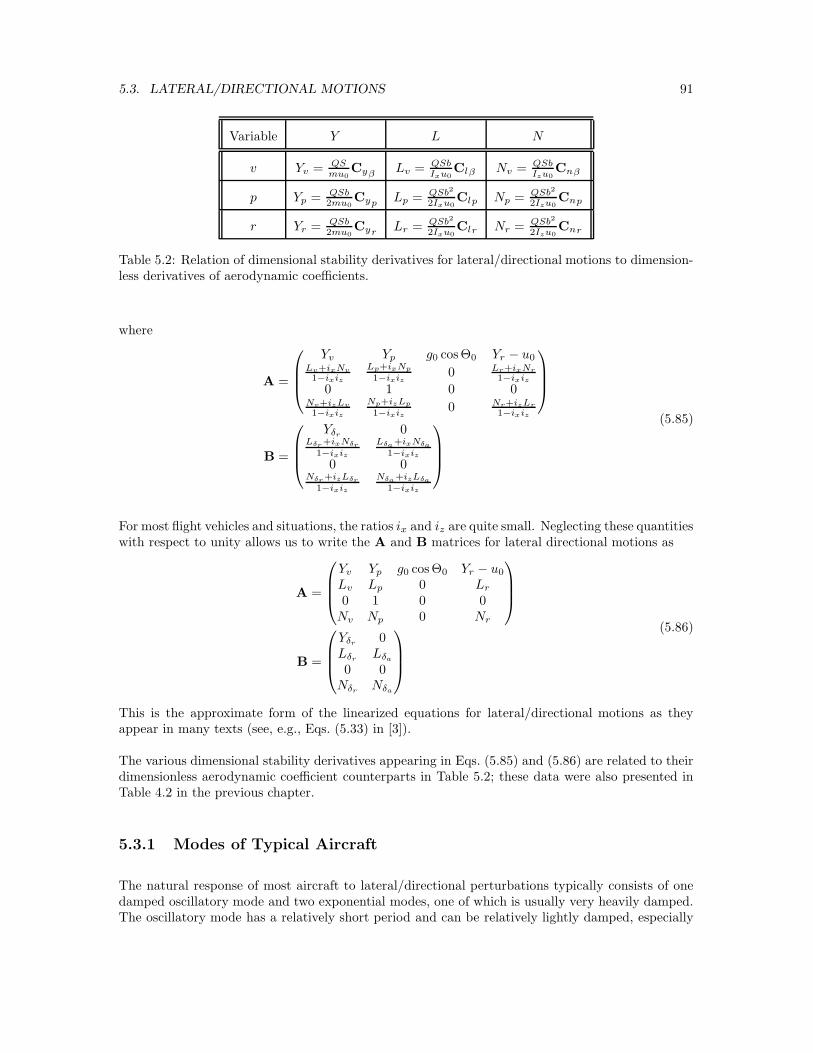
Variable Y L N
v Yv = QSmu0
Cyβ Lv = QSbIxu0
Clβ Nv = QSbIzu0
Cnβ
p Yp = QSb2mu0
Cyp Lp = QSb2
2Ixu0Clp Np = QSb2
2Izu0Cnp
r Yr = QSb2mu0
Cyr Lr = QSb2
2Ixu0Clr Nr = QSb2
2Izu0Cnr
Table 5.2: Relation of dimensional stability derivatives for lateral/directional motions to dimension-less derivatives of aerodynamic coefficients.
where
A =
Yv Yp g0 cosΘ0 Yr − u0Lv+ixNv
1−ixiz
Lp+ixNp
1−ixiz0 Lr+ixNr
1−ixiz
0 1 0 0Nv+izLv
1−ixiz
Np+izLp
1−ixiz0 Nr+izLr
1−ixiz
B =
Yδr0
Lδr +ixNδr
1−ixiz
Lδa+ixNδa
1−ixiz
0 0Nδr +izLδr
1−ixiz
Nδa+izLδa
1−ixiz
(5.85)
For most flight vehicles and situations, the ratios ix and iz are quite small. Neglecting these quantitieswith respect to unity allows us to write the A and B matrices for lateral directional motions as
A =
Yv Yp g0 cosΘ0 Yr − u0
Lv Lp 0 Lr
0 1 0 0Nv Np 0 Nr
B =
Yδr0
LδrLδa
0 0Nδr
Nδa
(5.86)
This is the approximate form of the linearized equations for lateral/directional motions as theyappear in many texts (see, e.g., Eqs. (5.33) in [3]).
The various dimensional stability derivatives appearing in Eqs. (5.85) and (5.86) are related to theirdimensionless aerodynamic coefficient counterparts in Table 5.2; these data were also presented inTable 4.2 in the previous chapter.
5.3.1 Modes of Typical Aircraft
The natural response of most aircraft to lateral/directional perturbations typically consists of onedamped oscillatory mode and two exponential modes, one of which is usually very heavily damped.The oscillatory mode has a relatively short period and can be relatively lightly damped, especially

92 CHAPTER 5. DYNAMIC STABILITY
for swept-wing aircraft; this is called the Dutch Roll mode, as the response consists of a combinedrolling, sideslipping, yawing motion reminiscent of a (Dutch) speed-skater. One of the exponentialmodes is very heavily damped, and represents the response of the aircraft primarily in roll; it iscalled the rolling mode. The second exponential mode, called the spiral mode, can be either stableor unstable, but usually has a long enough time constant that it presents no difficulty for pilotedvehicles, even when it is unstable.3
We illustrate this response again using the stability derivatives for the Boeing 747 aircraft at its Mach0.25 powered approach configuration at standard sea-level conditions. This is the same vehicle andtrim condition used to illustrate typical longitudinal behavior, and the basic aircraft properties andflight condition are given in Eq. (5.48). In addition, for the lateral/directional response we need thefollowing vehicle parameters
W = 564, 032. lbf, b = 195.7 ft
Ix = 14.3 × 10⁶ slug ft2, Iz = 45.3 × 10⁶ slug ft2, Ixz = −2.23× 10⁶ slug ft2 (5.87)
and the aerodynamic derivatives
Cyβ = −.96 Cyp = 0.0 Cyr = 0.0
Clβ = −.221 Clp = −.45 Clr = 0.101 (5.88)
Cnβ = 0.15 Cnp = −.121 Cnr = −.30
These values correspond to the following dimensional stability derivatives
Yv = −0.0999, Yp = 0.0, Yr = 0.0
Lv = −0.0055, Lp = −1.0994, Lr = 0.2468 (5.89)
Nv = 0.0012, Np = −.0933, Nr = −.2314
and the dimensionless product of inertia factors are
ix = −.1559, iz = −.0492 (5.90)
Using these values, the plant matrix is found to be
A =
−0.0999 0.0000 32.174 −279.10−0.0057 −1.0932 0.0 0.2850
0.0 1.0 0.0 0.00.0015 −.0395 0.0 −.2454
(5.91)
The characteristic equation is given by
|A − λI| = λ4 + 1.4385λ3 + 0.8222λ2 + 0.7232λ+ 0.0319 = 0 (5.92)
and its roots are
λDR = −.08066± ı 0.7433
λroll = −1.2308
λspiral = −.04641
(5.93)
3This is true at least when flying under visual flight rules and a horizontal reference is clearly visible. Underinstrument flight rules pilots must learn to trust the artificial horizon indicator to avoid entering an unstable spiral.
5.3. LATERAL/DIRECTIONAL MOTIONS 93
where, as suggested by the subscripts, the first pair of roots corresponds to the Dutch Roll mode,and the real roots corresponds to the rolling and spiral modes, respectively.
The damping ratio of the Dutch Roll mode is thus given by
ζDR =
√
√
√
√
1
1 +(
ηξ
)2
DR
=
√
1
1 +(
0.74330.08066
)2 = 0.1079 (5.94)
and the undamped natural frequency of the mode is
ωnDR=
−ξDR
ζDR=
0.08066
0.1079= 0.7477 sec−1 (5.95)
The period of the Dutch Roll mode is then given by
TDR =2π
ωn
√
1 − ζ2=
2π
0.7477√
1 − 0.10792= 8.45 sec (5.96)
and the number of cycles to damp to half amplitude is
N1/2DR
=ln 2
2π
√
1 − ζ2
ζ=
ln 2
2π
√1 − 0.10792
0.1079= 1.016 (5.97)
Thus, the period of the Dutch Roll mode is seen to be on the same order as that of the longitudinalshort period mode, but is much more lightly damped.
The times to damp to half amplitude for the rolling and spiral modes are seen to be
t1/2roll=
ln 2
−ξroll=
ln 2
1.2308= 0.563 sec (5.98)
and
t1/2spiral
=ln 2
−ξspiral=
ln 2
0.04641= 14.93 sec (5.99)
respectively.
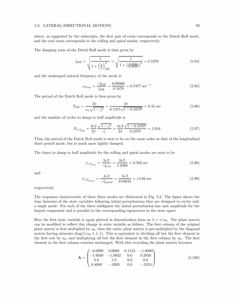
The responses characteristic of these three modes are illustrated in Fig. 5.8. The figure shows thetime histories of the state variables following initial perturbations that are designed to excite onlya single mode. For each of the three subfigures the initial perturbation has unit amplitude for thelargest component and is parallel to the corresponding eigenvector in the state space.
Here the first state variable is again plotted in dimensionless form as β = v/u0. The plant matrixcan be modified to reflect this change in state variable as follows. The first column of the originalplant matrix is first multiplied by u0, then the entire plant matrix is pre-multiplied by the diagonalmatrix having elements diag(1/u0, 1, 1, 1). This is equivalent to dividing all but the first element inthe first row by u0, and multiplying all but the first element in the first column by u0. The firstelement in the first column remains unchanged. With this re-scaling the plant matrix becomes
A =
−0.0999 0.0000 0.1153 −1.0000−1.6038 −1.0932 0.0 0.2850
0.0 1.0 0.0 0.00.4089 −.0395 0.0 −.2454
(5.100)

94 CHAPTER 5. DYNAMIC STABILITY
0 1 2 3 4 5 6 7 8 9 10
−1
−0.8
−0.6
−0.4
−0.2
0
0.2
0.4
0.6
0.8
1
Time, sec
Sta
te V
aria
ble
SideslipRoll rateRoll angleYaw rate
0 10 20 30 40 50 60 70 80 90 100−0.2
0
0.2
0.4
0.6
0.8
1
Time, sec
Sta
te V
aria
ble
SideslipRoll rateRoll angleYaw rate
0 2 4 6 8 10 12 14 16 18 20−1.5
−1
−0.5
0
0.5
1
1.5
Time, sec
Sta
te V
aria
ble
SideslipRoll rateRoll angleYaw rate
(a) Rolling mode (b) Spiral mode (c) Dutch Roll
Figure 5.8: Response of Boeing 747 aircraft to unit perturbation in eigenvectors corresponding tothe three lateral/directional modes of the vehicle. (a) Rolling mode; (b) Spiral mode; and (c) DutchRoll mode.
0 2 4 6 8 10 12 14 16 18 20−0.4
−0.2
0
0.2
0.4
0.6
0.8
1
1.2
Time, sec
Sta
te V
aria
ble
SideslipRoll rateRoll angleYaw rate
Figure 5.9: Response of Boeing 747 aircraft to unit perturbation in roll rate. Powered approach atM = 0.25 under standard sea-level conditions.
Note that, after this re-scaling, the magnitudes of the elements in the first row and first column ofthe plant matrix are more nearly the same order as the other terms (than they were in the originalform).
It is seen that the rolling mode consists of almost pure rolling motion (with a very small amountof sideslip). The spiral mode consists of mostly coordinated roll and yaw. And for the the DutchRoll mode, all the state variables participate, so the motion is characterized by coordinated rolling,sideslipping, and yawing motions.
An arbitrary initial perturbation will generally excite all three modes. This is illustrated in Fig. 5.9which plots the time histories of the state variables following an initial perturbation in roll rate. Theroll rate is seen to be quickly damped, leaving a slowly decaying spiral mode (appearing primarilyin the roll angle), with the oscillatory Dutch Roll mode superimposed.
The phasor plots for the rolling and spiral modes are relatively uninteresting, since these correspondto real roots. The eigenvector amplitudes, however, show that the rolling mode is dominated byperturbations in bank angle φ and roll rate p, with a very small amount of sideslip and negligibleyaw rate. The spiral mode is dominated by changes in bank angle. Since the motion is so slow,the roll rate is quite small, and the yaw rate is almost 2.5 times the roll rate, so we would expectsignificant changes in heading, as well as bank angle. The phasor diagram for the Dutch Roll mode
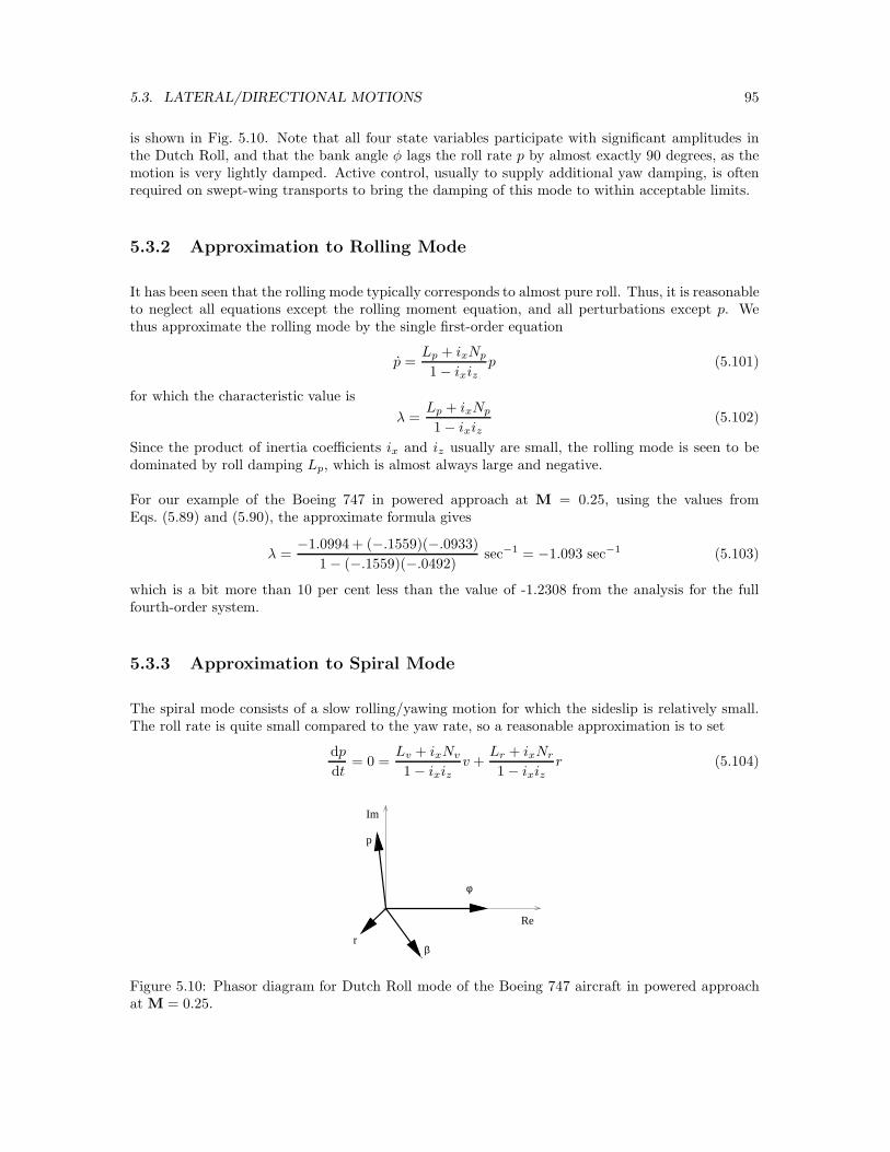
5.3. LATERAL/DIRECTIONAL MOTIONS 95
is shown in Fig. 5.10. Note that all four state variables participate with significant amplitudes inthe Dutch Roll, and that the bank angle φ lags the roll rate p by almost exactly 90 degrees, as themotion is very lightly damped. Active control, usually to supply additional yaw damping, is oftenrequired on swept-wing transports to bring the damping of this mode to within acceptable limits.
5.3.2 Approximation to Rolling Mode
It has been seen that the rolling mode typically corresponds to almost pure roll. Thus, it is reasonableto neglect all equations except the rolling moment equation, and all perturbations except p. Wethus approximate the rolling mode by the single first-order equation
p =Lp + ixNp
1 − ixizp (5.101)
for which the characteristic value is
λ =Lp + ixNp
1 − ixiz(5.102)
Since the product of inertia coefficients ix and iz usually are small, the rolling mode is seen to bedominated by roll damping Lp, which is almost always large and negative.
For our example of the Boeing 747 in powered approach at M = 0.25, using the values fromEqs. (5.89) and (5.90), the approximate formula gives
λ =−1.0994 + (−.1559)(−.0933)
1 − (−.1559)(−.0492)sec−1 = −1.093 sec−1 (5.103)
which is a bit more than 10 per cent less than the value of -1.2308 from the analysis for the fullfourth-order system.
5.3.3 Approximation to Spiral Mode
The spiral mode consists of a slow rolling/yawing motion for which the sideslip is relatively small.The roll rate is quite small compared to the yaw rate, so a reasonable approximation is to set
dp
dt= 0 =
Lv + ixNv
1 − ixizv +
Lr + ixNr
1 − ixizr (5.104)
φ
β
Im
Re
p
r
Figure 5.10: Phasor diagram for Dutch Roll mode of the Boeing 747 aircraft in powered approachat M = 0.25.

96 CHAPTER 5. DYNAMIC STABILITY
whence
v ≈ −Lr + ixNr
Lv + ixNvr (5.105)
Since ix and iz are generally very small, this can be approximated as
v ≈ −Lr
Lvr (5.106)
The yaw equationdr
dt=Nv + izLv
1 − ixizv +
Nr + izLr
1 − ixizr (5.107)
upon substitution of Eq. (5.106) and neglect of the product of inertia terms can then be written
dr
dt=
(
Nr −LrNv
Lv
)
r (5.108)
so the root of the characteristic equation for the spiral mode is
λ = Nr −LrNv
Lv(5.109)
Thus, it is seen that, according to this approximation, the spiral mode is stabilized by yaw dampingNr. Also, since stable dihedral effect corresponds to negative Lv and weathercock stability Nv androll due to yaw rate Lr are always positive, the second term in Eq. (5.109) is destabilizing; thusincreasing weathercock destabilizes the spiral mode while increasing dihedral effect stabilizes it.4
For our example of the Boeing 747 in powered approach at M = 0.25, using the values fromEqs. (5.89) and (5.90), the approximate formula gives
λ = −.2314− 0.2468
−.0055(0.0012) = −.178 (5.110)
which is almost four times the value of -.0464 from the analysis of the full fourth-order system. Thisis consistent with the usual difficulty in approximating small roots, but Eq. (5.109) still gives usefulqualitative information about the effects of weathercock and dihedral stability on the spiral mode.
5.3.4 Approximation to Dutch Roll Mode
The Dutch Roll mode is particularly difficult to approximate because it usually involves significantperturbations in all four state variables. The most useful approximations require neglecting eitherthe roll component or simplifying the sideslip component by assuming the vehicle c.g. travels in astraight line. This latter approximation means that ψ = −β, or
r = − v
u0(5.111)
The roll and yaw moment equations (neglecting the product of inertia terms ix and iz) can then bewritten as
d
dt
(
pr
)
=
(
Lv Lp Lr
Nv Np Nr
)
vpr
(5.112)
4Even if the spiral mode is unstable, its time constant usually is long enough that the pilot has no trouble counteringit. Unpiloted aircraft, however, must have a stable spiral mode, which accounts for the excessive dihedral usuallyfound on free-flight model aircraft.
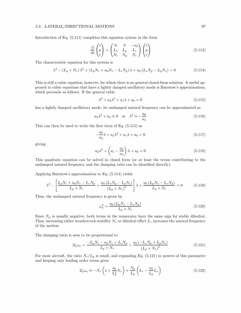
5.3. LATERAL/DIRECTIONAL MOTIONS 97
Introduction of Eq. (5.111) completes this equation system in the form
d
dt
vpr
=
0 0 −u0
Lv Lp Lr
Nv Np Nr
vpr
(5.113)
The characteristic equation for this system is
λ3 − (Lp +Nr)λ2 + (LpNr + u0Nv − LrNp)λ+ u0 (LvNp − LpNv) = 0 (5.114)
This is still a cubic equation, however, for which there is no general closed-form solution. A useful ap-proach to cubic equations that have a lightly damped oscillatory mode is Bairstow’s approximation,which proceeds as follows. If the general cubic
λ3 + a2λ2 + a1λ+ a0 = 0 (5.115)
has a lightly damped oscillatory mode, its undamped natural frequency can be approximated as
a2λ2 + a0 ≈ 0 or λ2 ≈ −a0
a2(5.116)
This can then be used to write the first term of Eq. (5.115) as
−a0
a2λ+ a2λ
2 + a1λ+ a0 = 0 (5.117)
giving
a2λ2 +
(
a1 −a0
a2
)
λ+ a0 = 0 (5.118)
This quadratic equation can be solved in closed form (or at least the terms contributing to theundamped natural frequency and the damping ratio can be identified directly).
Applying Bairstow’s approximation to Eq. (5.114) yields
λ2 −[
LpNr + u0Nv − LrNp
Lp +Nr+u0 (LvNp − LpNv)
(Lp +Nr)2
]
λ+u0 (LpNv − LvNp)
Lp +Nr= 0 (5.119)
Thus, the undamped natural frequency is given by
ω2n =
u0 (LpNv − LvNp)
Lp +Nr(5.120)
Since Np is usually negative, both terms in the numerator have the same sign for stable dihedral.Thus, increasing either weathercock stability Nv or dihedral effect Lv increases the natural frequencyof the motion.
The damping ratio is seen to be proportional to
2ζωn =−LpNr − u0Nv + LrNp
Lp +Nr+u0 (−LvNp + LpNv)
(Lp +Nr)2 (5.121)
For most aircraft, the ratio Nr/Lp is small, and expanding Eq. (5.121) in powers of this parameterand keeping only leading order terms gives
2ζωn ≈ −Nr
(
1 +u0
L2p
Nv
)
+Np
Lp
(
Lr −u0
LpLv
)
(5.122)
98 CHAPTER 5. DYNAMIC STABILITY
Yaw damping is thus seen to contribute to positive ζ and be stabilizing, and weathercock stabilityNv augments this effect. Since both Np and Lp usually are negative, however, the dihedral effect Lv
is seen to destabilize the Dutch Roll mode.5
For our example of the Boeing 747 in powered approach at M = 0.25, using the values fromEqs. (5.89) and (5.90), the approximate formulas give
ωn =
[
(279.1) [(−1.0994)(0.0012)− (−.0055)(−.0933)]
−1.0994− .2314sec−2
]1/2
= 0.620 sec−1 (5.123)
and
ζ = −(−1.0994)(−.2314)−(.2468)(−.0933)+(279.1)(0.0012)
−1.0994−.2314 + (279.1) (−.0055)(−.0933)−(−1.0994)(0.0012)(−1.0994−.2314)2
2(0.620)
= 0.138
(5.124)
The approximation for the undamped natural frequency is only about 15 per cent less than theexact value of 0.748, but the exact damping ratio of 0.1079 is over predicted by almost 30 per cent.Nevertheless, the approximate Eq. (5.122) gives useful qualitative information about the effect ofdihedral and weathercock on the damping of the mode.
5.3.5 Summary of Lateral/Directional Modes
We have seen that the response of a typical aircraft to lateral/directional perturbations consists oftwo exponential modes and one oscillatory mode:
1. A rolling mode that usually is heavily damped, whose time to damp to half amplitude isdetermined largely by the roll damping Lp;
2. A spiral mode that usually is only lightly damped, or may even be unstable. Dihedral effect isan important stabilizing influence, while weathercock stability is destabilizing, for this mode;and
3. A lightly damped oscillatory, intermediate frequency Dutch Roll mode, which consists of acoordinated yawing, rolling, sideslipping motion. For this mode, dihedral effect is generallydestabilizing, while weathercock stability is stabilizing.
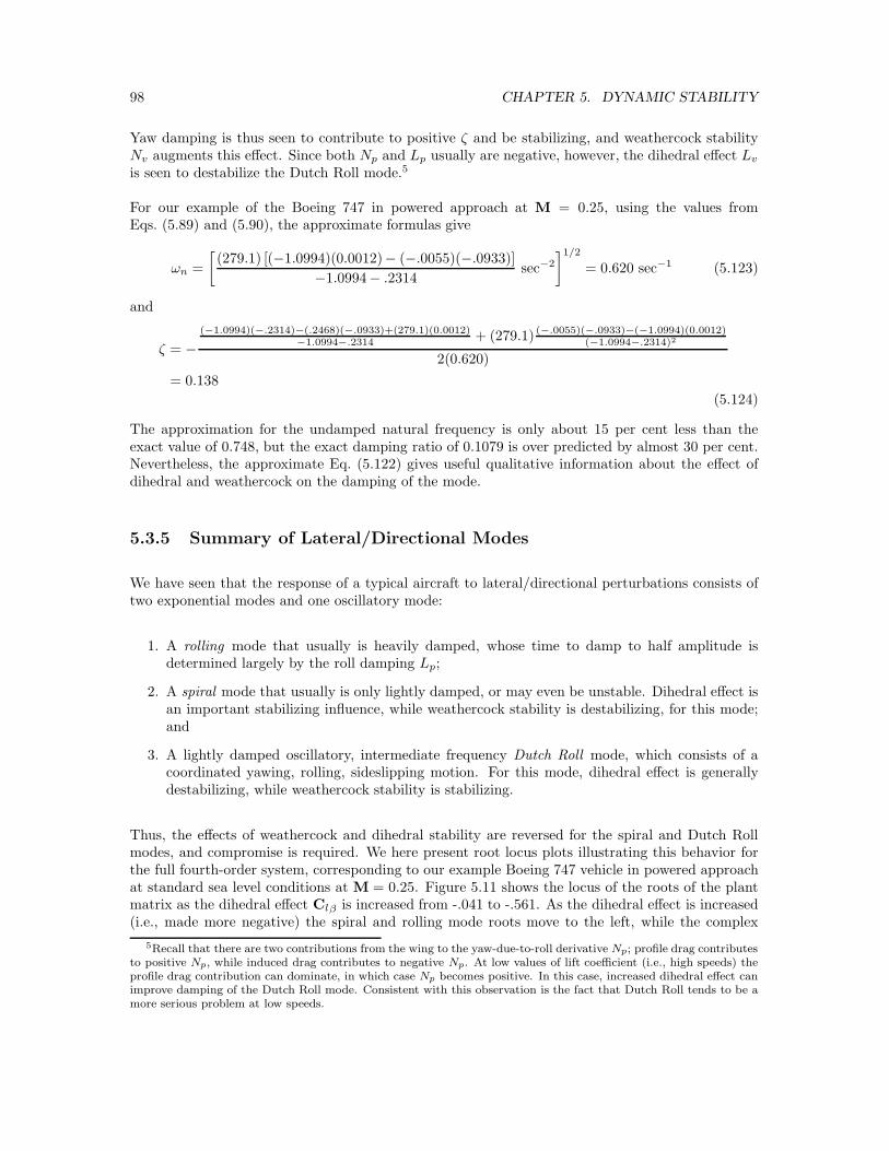
Thus, the effects of weathercock and dihedral stability are reversed for the spiral and Dutch Rollmodes, and compromise is required. We here present root locus plots illustrating this behavior forthe full fourth-order system, corresponding to our example Boeing 747 vehicle in powered approachat standard sea level conditions at M = 0.25. Figure 5.11 shows the locus of the roots of the plantmatrix as the dihedral effect Clβ is increased from -.041 to -.561. As the dihedral effect is increased(i.e., made more negative) the spiral and rolling mode roots move to the left, while the complex
5Recall that there are two contributions from the wing to the yaw-due-to-roll derivative Np; profile drag contributesto positive Np, while induced drag contributes to negative Np. At low values of lift coefficient (i.e., high speeds) theprofile drag contribution can dominate, in which case Np becomes positive. In this case, increased dihedral effect canimprove damping of the Dutch Roll mode. Consistent with this observation is the fact that Dutch Roll tends to be amore serious problem at low speeds.
5.3. LATERAL/DIRECTIONAL MOTIONS 99
-1
-0.5
0
0.5
1
-1.4 -1.2 -1 -0.8 -0.6 -0.4 -0.2 0
Imag
inar
y pa
rt o
f roo
t
Real part of root
Rolling modeDutch Roll Dutch Roll
Spiral mode
Figure 5.11: Locus of roots of plant matrix for Boeing 747 aircraft in powered approach at M = 0.25under standard sea-level conditions. Dihedral effect is varied from -.041 to -.561 in steps of -.04, whileall other stability derivatives are held fixed at their nominal values. Rolling and spiral modes becomeincreasingly stable as dihedral effect is increased; spiral mode becomes stable at approximatelyClβ = −.051. Dutch Roll mode becomes less stable as dihedral effect is increased and becomesunstable at approximately Clβ = −.532.
pair corresponding to the Dutch Roll mode moves to the right. Consistent with our approximateanalysis, increasing the dihedral effect is seen to increase the natural frequency of the Dutch Rollmode.
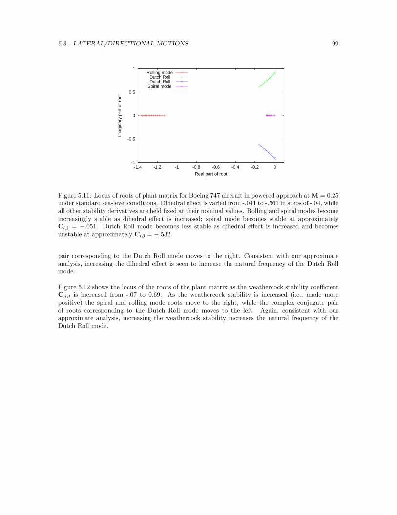
Figure 5.12 shows the locus of the roots of the plant matrix as the weathercock stability coefficientCnβ is increased from -.07 to 0.69. As the weathercock stability is increased (i.e., made morepositive) the spiral and rolling mode roots move to the right, while the complex conjugate pairof roots corresponding to the Dutch Roll mode moves to the left. Again, consistent with ourapproximate analysis, increasing the weathercock stability increases the natural frequency of theDutch Roll mode.
100 CHAPTER 5. DYNAMIC STABILITY
-1
-0.5
0
0.5
1
-1.2 -1 -0.8 -0.6 -0.4 -0.2 0
Imag
inar
y pa
rt o
f roo
t
Real part of root
Rolling modeDutch Roll Dutch Roll
Spiral mode
Figure 5.12: Locus of roots of plant matrix for Boeing 747 aircraft in powered approach at M = 0.25under standard sea-level conditions. Weathercock stability is varied from -.07 to 0.69 in steps of0.04, while all other stability derivatives are held fixed at their nominal values. Rolling and spiralmodes become less stable as weathercock stability is increased; spiral mode becomes unstable atapproximately Cnβ = 0.6567. Dutch roll mode becomes increasingly stable as weathercock stabilityis increased, but is unstable for less than about Cnβ = −.032.
5.4. STABILITY CHARACTERISTICS OF THE BOEING 747 101
5.4 Stability Characteristics of the Boeing 747
5.4.1 Longitudinal Stability Characteristics
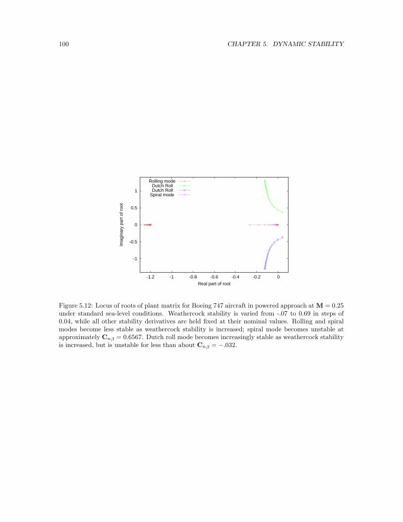
In this section we summarize the longitudinal mass distribution and aerodynamic stability charac-teristics of a large, jet transport aircraft, the Boeing 747, at selected flight conditions. Data aresummarized from the report by Heffley et al. [2]. Values for aerodynamic coefficients were scaleddirectly from plots of these variables, except for the derivatives CLq
and CLαfor which no data are
provided. These values were computed from the values of the corresponding dimensional stabilityderivatives Zq and Zw, which are provided in tabular form, with the sign of Zw changed to correcta seemingly obvious error.
Condition numbers correspond to those in the report; Conditions 5-10 are for a clean aircraft,Condition 2 corresponds to a powered approach with gear up and 20◦ flaps. Angles of attack arewith respect to the fuselage reference line.
Condition 2 5 7 9 10
h (ft) SL 20,000 20,000 40,000 40,000M∞ 0.25 0.500 0.800 0.800 0.900
α (degrees) 5.70 6.80 0.0 4.60 2.40W (lbf) 564,032. 636,636. 636,636. 636,636. 636,636.
Iy (slug-ft2) 32.3 × 10⁶ 33.1 × 10⁶ 33.1 × 10⁶ 33.1 × 10⁶ 33.1 × 10⁶
CL 1.11 0.680 0.266 0.660 0.521CD 0.102 0.0393 0.0174 0.0415 0.0415CLα
5.70 4.67 4.24 4.92 5.57CDα 0.66 0.366 0.084 0.425 0.527Cmα
-1.26 -1.146 -.629 -1.033 -1.613CLα
6.7 6.53 5.99 5.91 5.53Cmα
-3.2 -3.35 -5.40 -6.41 -8.82CLq
5.40 5.13 5.01 6.00 6.94Cmq
-20.8 -20.7 -20.5 -24.0 -25.1CLM
0.0 -.0875 0.105 0.205 -.278CDM
0.0 0.0 0.008 0.0275 0.242CmM
0.0 0.121 -.116 0.166 -.114CLδe
0.338 0.356 0.270 0.367 0.300Cmδe
-1.34 -1.43 -1.06 -1.45 -1.20
Table 5.3: Longitudinal mass properties and aerodynamic stability derivatives for the Boeing 747 atselected flight conditions.

102 CHAPTER 5. DYNAMIC STABILITY
5.4.2 Lateral/Directional Stability Characteristics
In this section we summarize the lateral/directional mass distribution and aerodynamic stabilitycharacteristics of a large, jet transport aircraft, the Boeing 747, at selected flight conditions. Dataare summarized from the report by Heffley et al. [2]. Values for aerodynamic coefficients were scaleddirectly from plots of these variables.
Condition numbers correspond to those in the report; Conditions 5-10 are for a clean aircraft,Condition 2 corresponds to a powered approach with gear up and 20◦ flaps. Moments and productsof inertia are with respect to stability axes for the given flight condition. Angles of attack are withrespect to the fuselage reference line.
Condition 2 5 7 9 10
h (ft) SL 20,000 20,000 40,000 40,000M∞ 0.25 0.500 0.800 0.800 0.900
α (degrees) 5.70 6.80 0.0 4.60 2.40W (lbf) 564,032. 636,636. 636,636. 636,636. 636,636.
Ix (slug-ft2) 14.3 × 10⁶ 18.4 × 10⁶ 18.2 × 10⁶ 18.2 × 10⁶ 18.2 × 10⁶
Iz (slug-ft2) 45.3 × 10⁶ 49.5 × 10⁶ 49.7 × 10⁶ 49.7 × 10⁶ 49.7 × 10⁶
Ixz (slug-ft2) −2.23 × 10⁶ −2.76× 10⁶ 0.97 × 10⁶ −1.56 × 10⁶ −.35 × 106
Cyβ-.96 -.90 -.81 -.88 -.92
Clβ -.221 -.193 -.164 -.277 -.095Cnβ
0.150 0.147 0.179 0.195 0.207Clp -.45 -.323 -.315 -.334 -.296Cnp
-.121 -.0687 0.0028 -.0415 0.0230Clr 0.101 0.212 0.0979 0.300 0.193Cnr
-.30 -.278 -.265 -.327 -.333Clδa
0.0461 0.0129 0.0120 0.0137 0.0139Cnδa
0.0064 0.0015 0.0008 0.0002 -.0027Cyδr
0.175 0.1448 0.0841 0.1157 0.0620Clδr
0.007 0.0039 0.0090 0.0070 0.0052Cnδr
-.109 -.1081 -.0988 -.1256 -.0914
Table 5.4: Lateral/Directional mass properties and aerodynamic stability derivatives for the Boeing747 at selected flight conditions.

Bibliography
[1] Bernard Etkin & Lloyd Duff Reid, Dynamics of Flight, Stability and Control, McGraw-Hill, Third Edition, 1996.
[2] R. K. Heffley & W. F. Jewell, Aircraft Handling Qualities Data, NASA CR-2144, December1972.
[3] Robert C. Nelson, Aircraft Stability and Automatic Control, McGraw-Hill, Second edi-tion, 1998.
[4] Louis V. Schmidt, Introduction to Aircraft Flight Dynamics, AIAA Education Series,1998.
103