What you should learn● Sketch graphs of equations

by point plotting.

● Graph equations using a

graphing utility.

● Use graphs of equations to solve

real-life problems.

Why you should learn itThe graph of an equation can help

you see relationships between

real-life quantities. For example,

in Exercise 66 on page B20, a graph

can be used to estimate the life

expectancies of children born in the

years 1948 and 2020.

The Graph of an EquationNews magazines often show graphs comparing the rate of inflation, the federal deficit,or the unemployment rate to the time of year. Businesses use graphs to report monthlysales statistics. Such graphs provide geometric pictures of the way one quantity changeswith respect to another. Frequently, the relationship between two quantities is expressedas an equation. This appendix introduces the basic procedure for determining the geometric picture associated with an equation.

For an equation in the variables and a point is a solution point when substitution of for and for satisfies the equation. Most equations have infinitelymany solution points. For example, the equation

has solution points

and so on. The set of all solution points of an equation is the graph of the equation.

Example 1 Determining Solution Points

Determine whether (a) and (b) lie on the graph of

Solution

a. Write original equation.

Substitute 2 for and 13 for

is a solution. ✓

The point does lie on the graph of because it is a solution pointof the equation.

b. Write original equation.

Substitute for and for

is not a solution.

The point does not lie on the graph of because it is not asolution point of the equation.

Now try Exercise 7.

The basic technique used for sketching the graph of an equation is the point-plottingmethod.

y � 10x � 7��1, �3�

��1, �3� �3 � �17

y.�3x�1 �3 �?

10��1� � 7

y � 10x � 7

y � 10x � 7�2, 13�

�2, 13� 13 � 13

y.x 13 �?

10�2� � 7

y � 10x � 7

y � 10x � 7.

��1, �3��2, 13�

�0, 5�, �1, 2�, �2, �1�, �3, �4�

3x � y � 5

ybxa�a, b�y,x

B12 Appendix B Review of Graphs, Equations, and Inequalities

B.2 Graphs of Equations

Sketching the Graph of an Equation by Point Plotting

1. If possible, rewrite the equation so that one of the variables is isolated on one side of the equation.

2. Make a table of values showing several solution points.

3. Plot these points on a rectangular coordinate system.

4. Connect the points with a smooth curve or line.

Appendix B.2 Graphs of Equations B13

Example 2 Sketching a Graph by Point Plotting

Use point plotting and graph paper to sketch the graph of

SolutionIn this case you can isolate the variable

Solve equation for

Using negative and positive values of and you can obtain the following tableof values (solution points).

Next, plot the solution points and connect them, as shown in Figure B.15. It appears thatthe graph is a straight line. You will study lines extensively in Section 1.1.

Now try Exercise 11.

The points at which a graph touches or crosses an axis are called the intercepts ofthe graph. For instance, in Example 2 the point

-intercept

is the -intercept of the graph because the graph crosses the -axis at that point. Thepoint

-intercept

is the -intercept of the graph because the graph crosses the -axis at that point.

Example 3 Sketching a Graph by Point Plotting

Use point plotting and graph paper to sketch the graph of

SolutionBecause the equation is already solved for make a table of values by choosing severalconvenient values of and calculating the corresponding values of

Next, plot the solution points, as shown in Figure B.16(a). Finally, connect the pointswith a smooth curve, as shown in Figure B.16(b). This graph is called a parabola. Youwill study parabolas in Section 2.1.

Now try Exercise 13.

In this text, you will study two basic ways to create graphs: by hand and using agraphing utility. For instance, the graphs in Figures B.15 and B.16 were sketched by hand,and the graph in Figure B.19 (on the next page) was created using a graphing utility.

y.xy,

y � x2 � 2.

xx

x�2, 0�

yy

y�0, 6�

x � 0,x,

y.y � 6 � 3x

y.

3x � y � 6.

x �1 0 1 2 3

y � 6 � 3x 9 6 3 0 �3

Solution point ��1, 9� �0, 6� �1, 3� �2, 0� �3, �3�

x �2 �1 0 1 2 3

y � x2 � 2 2 �1 �2 �1 2 7

Solution point ��2, 2� ��1, �1� �0, �2� �1, �1� �2, 2� �3, 7�

Figure B.15

(a)

(b)Figure B.16

B14 Appendix B Review of Graphs, Equations, and Inequalities

Using a Graphing UtilityOne of the disadvantages of the point-plotting method is that to get a good idea aboutthe shape of a graph, you need to plot many points. With only a few points, you couldmisrepresent the graph of an equation. For instance, consider the equation

When you plot the points and as shown inFigure B.17(a), you might think that the graph of the equation is a line. This is not correct. By plotting several more points and connecting the points with a smooth curve,you can see that the actual graph is not a line, as shown in Figure B.17(b).

(a) (b)Figure B.17

From this, you can see that the point-plotting method leaves you with a dilemma.This method can be very inaccurate when only a few points are plotted, and it is very time-consuming to plot a dozen (or more) points. Technology can help solve this dilemma. Plotting several (even several hundred) points on a rectangular coordinatesystem is something that a computer or calculator can do easily. For instance, you canenter the equation in a graphing utility (see Figure B.18) toobtain the graph shown in Figure B.19.

Figure B.18 Figure B.19

5−5

−10

10

y = x(x4 − 10x2 + 39)130

y �130x�x4 � 10x2 � 39�

�3, 3�,�1, 1�,�0, 0�,��1, �1�,��3, �3�,

y �1

30 x�x4 � 10x2 � 39�.

Using a Graphing Utility to Graph an Equation

To graph an equation involving and on a graphing utility, do the following.

1. Rewrite the equation so that is isolated on the left side.

2. Enter the equation in the graphing utility.

3. Determine a viewing window that shows all important features of the graph.

4. Graph the equation.

y

yx

Technology TipMany graphing utilitiesare capable of creatinga table of values such

as the following, which showssome points of the graph inFigure B.17(b). For instructionson how to use the table feature,see Appendix A; for specifickeystrokes, go to this textbook’sCompanion Website.

Technology TipBy choosing differentviewing windows for agraph, it is possible to

obtain very different impressionsof the graph’s shape. Forinstance, Figure B.20 shows adifferent viewing window forthe graph of the equation inFigure B.19. Note how FigureB.20 does not show all of theimportant features of the graph as does Figure B.19. Forinstructions on how to set up aviewing window, see AppendixA; for specific keystrokes, go tothis textbook’s CompanionWebsite.

Figure B.20

2−2

−2

2

y = x(x4 − 10x2 + 39)130

Appendix B.2 Graphs of Equations B15

Example 4 Using a Graphing Utility to Graph an Equation

To graph

enter the equation in a graphing utility. Then use a standard viewing window (seeFigure B.21) to obtain the graph shown in Figure B.22.

Figure B.21 Figure B.22

Now try Exercise 43.

Example 5 Using a Graphing Utility to Graph a Circle

Use a graphing utility to graph

SolutionThe graph of is a circle whose center is the origin and whose radius is 3.To graph the equation, begin by solving the equation for

Write original equation.

Subtract from each side.

Take the square root of each side.

Remember that when you take the square root of a variable expression, you mustaccount for both the positive and negative solutions. The graph of is theupper semicircle. The graph of is the lower semicircle. Enter bothequations in your graphing utility and generate the resulting graphs. In Figure B.23,note that for a standard viewing window, the two graphs do not appear to form a circle.You can overcome this problem by using a square setting, in which the horizontal and vertical tick marks have equal spacing, as shown in Figure B.24. On many graphing utilities, a square setting can be obtained by using a to ratio of 2 to 3. For instance,in Figure B.24, the to ratio is

Figure B.23 Figure B.24

Now try Exercise 57.

−4

−6 6

4

−10

−10 10

10

Ymax � Ymin

Xmax � Xmin�

4 � ��4�6 � ��6�

�8

12�

2

3.

xyxy

y � ��9 � x2y � �9 � x2

y � ±�9 � x2

x2 y2 � 9 � x2

x2 � y2 � 9

y.x2 � y2 � 9

x2 � y2 � 9.

10

−10

−10 10

y = − + 2xx3

2

y � �x3

2� 2x

Technology TipThe standard viewingwindow on manygraphing utilities does

not give a true geometric perspective because the screen isrectangular, which distorts theimage. That is, perpendicularlines will not appear to be perpendicular and circles willnot appear to be circular. Toovercome this, you can use asquare setting, as demonstratedin Example 5.

Technology TipNotice that when you graph a circle bygraphing two separate

equations for your graphingutility may not connect the twosemicircles. This is becausesome graphing utilities are limited in their resolution. So,in this text, a blue curve isplaced behind the graphing utility’s display to indicatewhere the graph should appear.

y,

B16 Appendix B Review of Graphs, Equations, and Inequalities

ApplicationsThroughout this course, you will learn that there are many ways to approach a problem.Two of the three common approaches are illustrated in Example 6.

An Algebraic Approach: Use the rules of algebra.

A Graphical Approach: Draw and use a graph.

A Numerical Approach: Construct and use a table.

You should develop the habit of using at least two approaches to solve every problemin order to build your intuition and to check that your answer is reasonable.

The following two applications show how to develop mathematical models to represent real-world situations. You will see that both a graphing utility and algebra canbe used to understand and solve the problems posed.

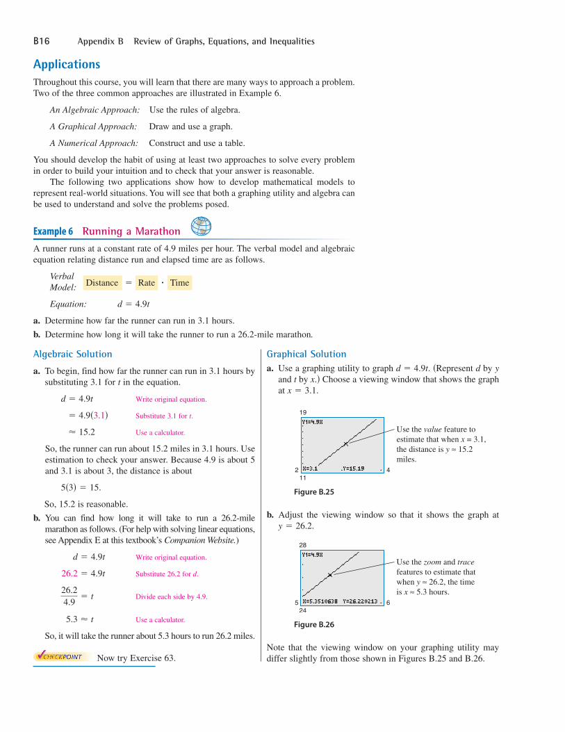
Example 6 Running a Marathon

A runner runs at a constant rate of 4.9 miles per hour. The verbal model and algebraicequation relating distance run and elapsed time are as follows.

Equation:

a. Determine how far the runner can run in 3.1 hours.

b. Determine how long it will take the runner to run a 26.2-mile marathon.

d � 4.9t

Time�Rate�DistanceVerbalModel:

Algebraic Solution

a. To begin, find how far the runner can run in 3.1 hours bysubstituting 3.1 for in the equation.

Write original equation.

Substitute 3.1 for

Use a calculator.

So, the runner can run about 15.2 miles in 3.1 hours. Useestimation to check your answer. Because 4.9 is about 5and 3.1 is about 3, the distance is about

So, 15.2 is reasonable.

b. You can find how long it will take to run a 26.2-milemarathon as follows. (For help with solving linear equations,see Appendix E at this textbook’s Companion Website.)

Write original equation.

Substitute 26.2 for

Divide each side by 4.9.

Use a calculator.

So, it will take the runner about 5.3 hours to run 26.2 miles.

Now try Exercise 63.

5.3 � t

26.24.9

� t

d. 26.2 � 4.9t

d � 4.9t

5�3� � 15.

� 15.2

t. � 4.9�3.1�

d � 4.9t

t

Graphical Solutiona. Use a graphing utility to graph Represent by

and by Choose a viewing window that shows the graphat

Figure B.25

b. Adjust the viewing window so that it shows the graph at

Figure B.26

Note that the viewing window on your graphing utility may differ slightly from those shown in Figures B.25 and B.26.

245 6

28

Use the zoom and tracefeatures to estimate thatwhen y ≈ 26.2, the timeis x ≈ 5.3 hours.

y � 26.2.

112 4

19

Use the value feature toestimate that when x = 3.1,the distance is y ≈ 15.2miles.

x � 3.1.x.�t

yd�d � 4.9t.

Appendix B.2 Graphs of Equations B17

Example 7 Monthly Wage

You receive a monthly salary of $2000 plus a commission of 10% of sales. The verbalmodel and algebraic equation relating the wages, the salary, and the commission are asfollows.

Equation:

a. Sales are $1480 in August. What are your wages for that month?

b. You receive $2225 for September. What are your sales for that month?

Remember to use a different approach to check that your answer is reasonable. Forinstance, to check the numerical solution to Example 7, use a graphical approach asshown above or use an algebraic approach as follows.

a. Substitute 1480 for in the original equation and solve for

b. Substitute 2225 for in the original equation and solve for

x � $22502225 � 2000 � 0.1x

x.y

y � 2000 � 0.1�1480� � $2148

y.x

y � 2000 � 0.1x

Commission on sales�Salary�WagesVerbalModel:

Numerical Solutiona. Enter in a graphing utility. Then use

the table feature of the graphing utility to create a table.Start the table at with a table step of 10.

b. Adjust the table to start at with a table step of100.

You can improve the estimate by starting the table atwith a table step of 10.

Now try Exercise 65.

From the table, youcan see that wages of$2225 result fromsales of $2250.

x � 2200

From the table, youcan see that wages of$2225 result fromsales between $2200and $2300.

x � 2000

When x = 1480, thewages are y = $2148.

x � 1400

y � 2000 � 0.1x

Graphical Solutiona. Use a graphing utility to graph Choose a

viewing window that shows the graph at

b. Use the graphing utility to find the value along the axis(sales) that corresponds to a value of 2225 (wages). Adjustthe viewing window so that it shows the graph at

15001000 3350

3050

Use the zoom and tracefeatures to estimate thatwhen y = 2225, the salesare x = $2250.

y � 2225.y-

x-

10000 2000

3000

Use the value featureto estimate that whenx = 1480, the wagesare y = $2148.

x � 1480.y � 2000 � 0.1x.

B18 Appendix B Review of Graphs, Equations, and Inequalities

B.2 Exercises For instructions on how to use a graphing utility, see Appendix A.

Determining Solution Points In Exercises 5–10,determine whether each point lies on the graph of theequation.

Equation Points

5. (a) (b)

6. (a) (b)

7. (a) (b)

8. (a) (b)

9. (a) (b)

10. (a) (b)

Sketching a Graph by Point Plotting In Exercises 11–14,complete the table. Use the resulting solution points tosketch the graph of the equation. Use a graphing utilityto verify the graph.

11.

12.

13.

14.

Matching an Equation with Its Graph In Exercises15–18, match the equation with its graph. [The graphsare labeled (a), (b), (c), and (d).]

(a) (b)

(c) (d)

15. 16.17. 18.

Sketching the Graph of an Equation In Exercises 19–32,sketch the graph of the equation.

19. 20.

21. 22.

23. 24.

25. 26.

27. 28.

29. 30.

31. 32. x � y 2 � 4x � y2 � 1

y � 4 � �x�y � �x � 2�y � �1 � xy � �x � 3

y � x3 � 3y � x3 � 2

y � �x2 � 4xy � x2 � 3x

y � x2 � 1y � 2 � x2

y � 2x � 3y � �4x � 1

y � �x� � 3y � �9 � x2

y � 4 � x2y � 2�x

−6

−3

6

5

−6

−4

6

4

−2

−1

10

7

−6

−5

6

3

6x � 2y � �2x2

2x � y � x2

8x � 4y � 24

3x � 2y � 2

��3, 9��2, �163 �y �

13 x3 � 2x2

��4, 2��3, �2�x2 � y 2 � 20

�1, �1��1, 2�2x � y � 3 � 0

�1.2, 3.2��1, 5�y � 4 � �x � 2���2, 8��2, 0�y � x2 � 3x � 2

�12, 4��0, 2�y � �x � 4

Vocabulary and Concept CheckIn Exercises 1 and 2, fill in the blank.

1. For an equation in and if substitution of for and for satisfies the equation, then the point is a _______ .

2. The set of all solution points of an equation is the _______ of the equation.

3. Name three common approaches you can use to solve problems mathematically.

4. List the steps for sketching the graph of an equation by point plotting.

Procedures and Problem Solving

�a, b�ybxay,x

x �2 023 1 2

y

Solution point

x �1 0 1 2 3

y

Solution point

x �3 �1 0 2 3

y

Solution point

x �4 �3 �2 0 1

y

Solution point

Appendix B.2 Graphs of Equations B19

Using a Graphing Utility to Graph an Equation InExercises 33–46, use a graphing utility to graph theequation. Use a standard viewing window. Approximateany - or -intercepts of the graph.

33. 34.

35. 36.

37. 38.

39.

40.

41.

42.

43.

44.

45.

46.

Describing the Viewing Window of a Graphing Utility InExercises 47 and 48, describe the viewing window of thegraph shown.

47. 48.

Verifying a Rule of Algebra In Exercises 49–52, explainhow to use a graphing utility to verify that Identify the rule of algebra that is illustrated.

49. 50.

51. 52.

Using a Graphing Utility to Graph an Equation InExercises 53–56, use a graphing utility to graph theequation. Use the trace feature of the graphing utility toapproximate the unknown coordinate of each solutionpoint accurate to two decimal places. (Hint: You mayneed to use the zoom feature of the graphing utility toobtain the required accuracy.)

53. 54.

(a) (a)

(b) (b)

55. 56.

(a) (a)

(b) (b)

Using a Graphing Utility to Graph a Circle In Exercises57–60, solve for and use a graphing utility to graph eachof the resulting equations in the same viewing window.(Adjust the viewing window so that the circle appearscircular.)

57. 58.

59.

60.

Determining Solution Points In Exercises 61 and 62,determine which point lies on the graph of the circle.(There may be more than one correct answer.)

61.

(a) (b)

(c) (d)

62.

(a) (b)

(c) (d) ��1, 3 � 2�6 ��1, �1��0, 0���2, 3�

�x � 2�2 � �y � 3�2 � 25

�0, 2 � 2�6 ��5, �1���2, 6��1, 3�

�x � 1�2 � �y � 2�2 � 25

�x � 3�2 � �y � 1�2 � 25

�x � 1�2 � �y � 2�2 � 9

x2 � y2 � 36x2 � y2 � 16

y

�x, 1.5��x, �4��2, y���0.5, y�

y � �x2 � 6x � 5�y � x5 � 5x

�x, 20��x, 3��2.25, y��3, y�

y � x3�x � 3�y � �5 � x

y2 � 1y2 � 2�x2 � 1�

y1 � �x � 3� �1

x � 3y1 �

1

5�10�x2 � 1��

y2 �32x � 1y2 �

14x2 � 2

y1 �12x � �x � 1�y1 �

14�x2 � 8�

y1 � y2.

y � �x � 2 � 1y � �10x � 50

x3 � y � 1

y � 4x � x2�x � 4�2y � x2 � 8 � 2x

x2 � y � 4x � 3

y � 3�x � 1

y � 3�x � 8

y � �6 � x��x

y � x�x � 3

y �6

xy �

2x

x � 1

y �23x � 1y � 3 �

12 x

y � x � 1y � x � 7

yx

63. MODELING DATAA manufacturing plant purchases a new moldingmachine for $225,000. The depreciated value (decreasedvalue) after years is for

(a) Use the constraints of the model and a graphingutility to graph the equation using an appropriateviewing window.

(b) Use the value feature or the zoom and tracefeatures of the graphing utility to determine thevalue of when Verify your answer algebraically.

(c) Use the value feature or the zoom and tracefeatures of the graphing utility to determine the value of when Verify your answer algebraically.

t � 2.35.y

t � 5.8.y

0 � t � 8.y � 225,000 � 20,000t,ty

64. MODELING DATAYou buy a personal watercraft for $8100. The depreciated value after years is for

(a) Use the constraints of the model and a graphingutility to graph the equation using an appropriateviewing window.

(b) Use the zoom and trace features of the graphing utility to determine the value of when

Verify your answer algebraically.

(c) Use the value feature or the zoom and trace featuresof the graphing utility to determine the value of when Verify your answer algebraically.t � 5.5.

y

y � 5545.25.t

0 � t � 6.y � 8100 � 929t,ty

B20 Appendix B Review of Graphs, Equations, and Inequalities

66. (p. B12) The table showsthe life expectancy of a child (at birth) in the UnitedStates for each of the selected years from 1930 through2000. (Source: U.S. National Center for HealthStatistics)

A model that represents the data is given by

where is the time in years, with corresponding to1930.

(a) Use a graphing utility to graph the data from the tableabove and the model in the same viewing window.How well does the model fit the data? Explain.

(b) Find the -intercept of the graph of the model. Whatdoes it represent in the context of the problem?

(c) Use the zoom and trace features of the graphing utility to determine the year when the life expectancywas 73.2. Verify your answer algebraically.

(d) Determine the life expectancy in 1948 both graphically and algebraically.

(e) Use the model to estimate the life expectancy of achild born in 2020.

ConclusionsTrue or False? In Exercises 67 and 68, determine whetherthe statement is true or false. Justify your answer.

67. A parabola can have only one -intercept.

68. The graph of a linear equation can have either no -intercepts or only one -intercept.

69. Writing Your employer offers you a choice of wagescales: a monthly salary of $3000 plus commission of7% of sales or a salary of $3400 plus a 5% commission.Write a short paragraph discussing how you wouldchoose your option. At what sales level would theoptions yield the same salary?

70. Finance You open a savings account and deposit$200. Every week you withdraw $50. The account balance after weeks is for

(a) Use point plotting and graph paper to sketch thegraph of

(b) Use a graphing utility to graph

(c) Explain how to find an appropriate viewing window for the graph of the equation.

(d) Find the -intercept of the graph of the model. Whatdoes it represent in the context of the problem?

y

y � �50t � 200.

y � �50t � 200.

0 � t � 4.y � �50t � 200,ty

xx

x

y

t � 0t

0 � t � 70y �59.617 � 1.18t

1 � 0.012t,

y

The table shows the median (middle) sales prices (inthousands of dollars) of new one-family homes in thesouthern United States from 2000 through 2008.(Sources: U.S. Census Bureau; U.S. Department ofHousing and Urban Development)

A model that represents the data is given by

where represents the year, with correspondingto 2000.

(a) Use the model and the table feature of a graphingutility to find the median sales prices from 2000through 2008. How well does the model fit thedata? Explain.

(b) Use the graphing utility to graph the data from thetable and the model in the same viewing window.How well does the model fit the data? Explain.

(c) Use the model to estimate the median sales pricesin 2012 and 2014. Do the values seem reasonable?Explain.

(d) Use the zoom and trace features of the graphing utility to determine during which year(s) the median sales price was approximately $150,000.

t � 0t0 � t � 8,y � �0.4221t3 � 4.690t2 � 3.47t � 150.9,

y

65. MODELING DATA

Year Median sales price, y

2000 148.02001 155.42002 163.42003 168.12004 181.12005 197.32006 208.22007 217.72008 203.7

Year Life expectancy, y

1930 59.71940 62.91950 68.21960 69.71970 70.81980 73.71990 75.42000 77.0