Page 1/22

Longitudinal variations of noontime thermosphericwinds in response to IMF Bz temporal oscillations:broken mean circulation and standing featureKedeng Zhang  ( Ninghe_zkd@whu.edu.cn )

wuhan University https://orcid.org/0000-0003-2423-7419Hui Wang 

Wuhan University https://orcid.org/0000-0001-8459-5213Wenbin Wang 

High Altitude Observatory, National Center for Atmospheric ResearchJing Liu 

High Altitude Observatory, National Center for Atmospheric ResearchJie Gao 

Wuhan University

Research article

Keywords: Periodic oscillation of IMF Bz, Modeling and forecasting, thermospheric winds, Standingfeature, longitudinal differences

Posted Date: January 18th, 2021

DOI: https://doi.org/10.21203/rs.3.rs-46709/v4

License: This work is licensed under a Creative Commons Attribution 4.0 International License.  Read Full License

Page 2/22

AbstractBy using the coupled magnetosphere-thermosphere-ionosphere model, we explore the longitudinal/UTdependences of the dayside neutral wind in response to the 60 min periodic oscillation of theinterplanetary magnetic �eld (IMF) Bz. The southward propagation of the traveling atmosphericdisturbances (TADs) in meridional wind stands at about 20º MLat, which is related to the geomagnetic�eld con�guration, neutral temperature, and electron density changes. The meridional wind travelscontinuously from high to low latitude in the western southern hemisphere, with several sudden changesin the wave phase along the propagation direction. The broken mean circulation that is induced by theinteraction between TADs and simultaneous responses of the meridional winds driven by oscillating solarwind conditions is induced by the stronger roles of the ion drag than the pressure gradient. Note here thatthe mean circulation is the background meridional winds in the base case with the IMF Bz setting to zeroin the CMIT model. The ion drag shows obvious longitudinal differences associated with the penetrationof the ionospheric electric �eld during the oscillation of IMF Bz. 

IntroductionThe energy carried by the solar wind can be deposited into the Earth’s upper thermosphere at highlatitudes, and produce longitudinally extended disturbances (Bruinsma et al., 2007, 2009; Liu et al.,2018b). These waves then propagate away from the source region to other regions of the coupledIonosphere-Thermosphere (IT) system. These waves are named as traveling atmospheric disturbances(TADs), which are a key factor in understanding the variability of the IT system. Exploring the possiblemechanisms of TADs is critical in the modeling and forecasting of near-Earth upper atmosphereenvironment. 

In the past decades, TADs during disturbed periods have attracted much attention (e.g., Bruinsma &Forbes, 2007; Liu and Lühr, 2005; Liu et al., 2010, 2014, 2018b; Oliveira et al., 2017; Otsuka et al., 2004;Shiokawa et al., 2003; Sutton et al., 2009; Thome et al., 1964; Zhang et al., 2019). Previous studies havereported that the storm time energetic particle precipitation and Joule heating (Rodríguez-Zuluaga et al.,2016), the gravity waves (Liu et al., 2014), and the sunset terminator (Beer, 1973) are critical in thegeneration of TADs. The storm time energy deposition can signi�cantly increase the neutral temperatureat high latitudes, changing the global circulation and triggering the TADs via the pressure gradient force.The upward propagating gravity waves, which are ubiquitous in the mesosphere and lower thermosphere,and atmospheric waves that are associated with the sunset terminator, can deposite energy andmomentum at higher altitudes. This energy deposition also plays a role in the neutral temperaturechanges in the thermosphere, and cause TADs. 

As reported by Dungey (1961), the geomagnetic storms can be induced by the interaction between theIMF Bz in southward and the geomagnetic �eld. During disturbed periods, a large amount of energy andmomentum carried by the solar wind is deposited into the Earth’s upper atmosphere, changing the globalcirculation and producing TADs. TADs have been studied using meridional winds, neutral temperature,

Page 3/22

composition (O/N2), and air mass density data (e.g., Bruinsma and Forbes, 2007; Bruinsma et al., 2009;Fujiwara et al., 2006; Lei et al., 2008). Typically, TADs propagate with velocities of 400-1000 (100-300)m/s, periods of 0.5-3 (0.25-1) hour, and wavelength of thousands (hundreds) of kilometers in large-scales(medium-scales) (e.g., Bruinsma and Forbes, 2009; Hocke and Schlegel, 1996). 

Liu and Lühr (2005) found that during storm times the enhancement of the thermospheric air massdensity in the noontime showed two different features (see the upper panel of Figure 3 in Liu and Lühr,2005). One was the enhancement in the density at 0º~40º geomagnetic latitudes (MLat), whichoriginated from the TAD propagating from the auroral region to low latitudes at around 20 UT on 30October 2003. The other was the almost instant enhancement in the density from aurora to middlelatitudes at about 20:00 UT on 30 October 2003. These two features overlapped at 20:00 UT and 40ºMLat, forming broken mean circulation. This broken feature and its possible mechanisms have rarelybeen studied in the literature, which is one of the focus of the study. 

Another interesting topic is raised by Sharma et al. (2011). They reported a longitudinal variation of thestorm time O/N2 enhancement during the geomagnetic storm of 15 May 2005: it was stronger at Yibal(22.18º Geographic latitude (GLat), 56.11º Geographic longitude (GLon)) than at Kunming (25.03º GLat,102.79º GLon) and Udaipur (24.67º GLat, 74.69º GLon). This longitudinal variation was attributed to theair upwelling due to the equatorward meridional wind (Sharma et al., 2011). One remaining question isthen whether TADs in the meridional wind also show notable longitudinal variations? Based onobservations from all-sky airglow imagers, Otsuka et al. (2004) investigated the geomagnetic conjugacyof the medium-scale traveling ionospheric disturbances (TID). The conjugacy structures came from thepolarization electric �eld that maps along geomagnetic �eld lines and moves the F region plasmaupward/downward, producing the trans-hemispheric structures of plasma perturbations in the Northernand Southern Hemispheres. TID can be treated as the ionospheric counterpart of TAD always with phaseand time delay compared to TAD. Thus, the hemispheric conjugacy of the TAD is worthy of investigation.

While the TADs in thermospheric winds during storm time have been established in the literature, theexact longitudinal and hemispheric changes of the meridional wind responses to temporal oscillations ofIMF Bz is still poorly understood, due to the fact that the thermospheric winds are balanced among manydrivers (i.e., pressure gradient, ion drag, Coriolis force). The thermospheric winds are important factors inthe understanding of changes in the ionosphere-thermosphere coupling system. In addition, the periodicoscillations of IMF Bz are a common phenomenon seen in the solar wind, which can produce periodicoscillations in the energy and momentum deposition in the upper atmosphere and TADs (e.g., Liu et al.,2018a; Zhang et al., 2019). The TAD and simultaneous responses in meridional winds driven byoscillating solar wind conditions are different phenomena, and it is not unusual that different phenomenaoccur simultaneously in thermosphere. As shown in Figure 1c in our result and upper panel of Figure 3 inLiu and Lühr, 2005, those two features interacted with each other. Because the simultaneous response ofmass density, as indicated by the vertical arrow, also has a character of interhemispheric asymmetry thatit occurs at earlier time in the Southern Hemisphere than that in the Northern Hemisphere. Note here thatthe ionospheric parameters are modulated by the prompt penetrating electric �eld immediately in global

Page 4/22

scale. Thus, there should be no signi�cant time delay between different hemispheres. The TAD mightaccount for the time differences, via the processes of pushing neutrals to lower latitudes with time delaywith respect to latitudes. To summarize, it is a physical interesting and true phenomenon, and deserves tobe furtherly explored. This physical interesting phenomenon has never caught any attentions in theliterature, and reported at �rst time. In order to simplify the description in the following, it is named as“broken mean circulation” in our work. Taking the abovementioned description into consideration, thepresent work is to study the longitudinal and hemispheric patterns of the meridional wind changes at a�xed local time, which show some interesting signals of the broken mean circulation, standing feature,and the related longitudinal and hemispheric variations during the period of the oscillating IMF Bz.Furthermore, these thermospheric wind changes have not caught so much attention in the literature. Thepossible drivers for the noontime wind changes are revealed, including the possible effects of thegeomagnetic topology. Electron density, plasma motion, and neutral temperature changes are alsoexamined. 

MethodsCHAMP Data

The orbit of the CHAllenging Minisatellite Payload (CHAMP) satellite was near-polar (87.3º inclination)(Reigber et al., 2002). The orbital period of CHAMP was about 93 min. The initial orbital altitude was 460km in 2000, then decreased to about 400 km in 2005 and about 300 km in 2008 due to atmospheric drag.The neutral air density data is deduced from the measurements by the accelerometer on board theCHAMP (Doornbos E., 2012). In this work, the observed mass density data at geographic latitudes of-60º~60º are processed according to the orbit-by-orbit method, similar to the method using in Häusler etal. (2007). The mass density in previous orbit are removed to represent the mass density disturbances incurrent orbit.

 CMIT Model

The Coupled Magnetosphere Ionosphere Thermosphere (CMIT) model consists of two parts. One is theThermosphere Ionosphere Electrodynamic General Circulation Model (TIEGCM) v1.95, the other is theLyon–Fedder–Mobarry (LFM) global magnetohydrodynamic magnetospheric model (Wang et al., 2004;Wiltberger et al., 2004). When investigating the coupling in the MIT system, the model outputs haveachieved good agreements with observations and other model outputs, con�rming the reliability andstability of CMIT (e.g., Cnossen & Richmond, 2013; Liu et al., 2018a; Wang et al., 2008). The TIEGCM is athree-dimensional, time-dependent model of the coupled IT system. The drivers of TIEGCM are shown asfollow: the particle precipitation and high-latitude electric �elds (Heelis et al., 1982), solar extremeultraviolet and ultraviolet spectral �uxes (Richards et al., 1994), the upward-propagating atmospherictides (Hagan & Forbes., 2002, 2003). Note here that the atmospheric tides, including migrating andnonmigrating tides, are either speci�ed by the global scale wave model or derived from the Sounding ofthe Atmosphere using Broadband Emission Radiometry (SABER) and TIDI observations. The TIEGCM has

Page 5/22

a horizontal resolution of 2.5º GLat × 2.5º GLon, and a vertical resolution of quarter-scale height with 57levels. The model extends from ~97 km to ~600 km in the vertical direction, with the upper boundarydepending on the solar activity. As revealed by Lyon et al. (2004), the drivers of LFM Magnetospheremodel are the solar wind and IMF data, and the boundary of LFM extends from -300 RE to 2RE. The RE isthe Earth’s radius. In the coupled MIT system, the modeled ionospheric conductivity from TIEGCM isimposed into the LFM, and the simulated auroral particle precipitation and high-latitude electric �eldsfrom the LFM are used to drive the TIEGCM. 

In this study, the changes in the IT system due to the effects of IMF Bz oscillation are explored byperforming two CMIT simulations. One is the 60-min case that Bz varies with a maximum amplitude of10 nT (from -10 nT to 10 nT) and a sine function of a period of 60 min, the other is the CMIT base runwith a constant Bz value of 0 nT. The hemispheric power, joule heating, and partial precipitation oscillateas well (Figures not shown). The auroral oval (size and locations) change in a similar way to the particleprecipitation. The electric �eld penetration also oscillates with a similar amplitude as observed (Figuresnot shown, Wei et al., 2008). As reported by Wei et al. (2008), the penetrating electric �eld oscillates withthe variations of IMF Bz. The maximum amplitude of the penetrating electric �elds at Jicamarca (11.9ºSGLAT, 76.8ºW GLON) is ~1 mv/m in their case. In our simulations, the maximum PPEF is ~3 mv/m(Figure not shown), which might be overestimated (Merkin et al., 2005; Wang et al., 2008). As shown inthe previous work of Zhang et al. (2019), the disturbed wind in the oscillation period of 60 minutes in IMFBz is strongest when compared to the other two cases with an oscillation period of 10 and 30 minutes.Thus, in the present work, we will focus on the 60-min case. In addition, the other input solar windconditions for CMIT are solar wind density (5 cm-3), velocity (400 km/s), IMF Bx and By (both are 0 nT).To show the thermospheric responses to IMF oscillation, the background winds giving in CMIT base runare removed. 

ResultsBroken Mean Circulation

Figure 1a is the UT variation of IMF Bz on Nov 11, 2003, which oscillated between northward andsouthward directions with periods from tens of minutes to several hours. The IMF data comes from theACE spacecraft at L1 (Lagrange point) point downloaded from the OMNI website(https://omniweb.gsfc.nasa.gov/). The observed Bz variations on Nov 11, 2003 have temporaloscillations, with similar period and magnitude as modeled ones. Figure 1b shows the neutral densities at~12 LT observed by CHAMP on Nov 11, 2003 at middle and low latitudes. Note here that the neutraldensity during quiet times (Nov. 8, 2003, Kp = 1.8) is removed as the background. The x-axis in Figure 1balso denotes the latitudes of CHAMP orbits. The disturbances in neutral density are the spatial variationof CHAMP observations. Due to the lack of meridional winds observed by CHAMP, the neutral densitiesare used to represent TADs. In Figure 1b, the disturbed neutral density shows two different features (orbit1 denotes the background mass density under quiet condition). One is the disturbed density occurring atalmost the same time at -60º~-30º geographic latitudes (GLat) at 05 UT on Nov. 11, 2003 (see orbit 2).

Page 6/22

The density changes at -60º~-30º geographic latitudes (GLat) are much stronger at orbit 2 than that atother orbits. Note that the CHAMP satellite has a speed of 7.6 km/s, which is much faster than thepropagation of TADs. Thus, the density changes at orbit 2 can be regarded as a response withoutsigni�cant time delay at latitudes. The other is the propagation of the density disturbance from -30º GLatto -10º GLat in ~2 hours, with a phase speed of ~300 m/s (magenta arrows in Figure 1b). The densitychanges at orbit 3 and -30º~-10º GLat are enhanced, which could be propagated from high latitudes asobserved at orbit 2. These two features demonstrate the broken mean circulation as shown in Figures 1band 1c. Figure 1c is the universal time changes of neutral mass density observed by CHAMP, as reportedin Figure 3 of Liu and Lühr (2005). The broken mean circulation structure is indicated by the black arrows.The TADs in neutral density propagates equatorward from ~60° GLat at 17 UT to 20° GLat at 20 UT. Inaddition, the neutral density at -60° ~ 20° GLat seems to be enhanced at almost the same time. However,an interhemispheric asymmetry of the UT of the simultaneous response peaks occurs, which is attributedto the interaction between TAD and simultaneous responses in the Northern Hemisphere. This interactionpromotes the later UT in the Northern Hemisphere than that in the Southern Hemisphere. As known to all,the �ow of neutrals forms the thermospheric winds. Thus, the temporal and spatial variations of zonalwinds represent the zonal motion of neutrals, while the meridional winds denote the equatorward orpoleward �ow of neutrals. For the lack of meridional wind observations from satellite, the TADs andsimultaneous responses in meridional winds can be observed in the mass density in an indirect andsimilar style. Moreover, during the storm period (29-31 Oct, 2003), the electron density also exhibited anevident combined feature of traveling ionospheric disturbances (TIDs) and the simultaneous responses(Figure 1d). The electron density at 40º ~ 70º (-40º ~ -60º) GLat in the Northern (Southern) Hemisphereincreases at almost the same time, as indicated by the vertical black arrows. Then, the enhancementtravelled to low latitudes in ~4 hours (the sloped black arrows).

The broken mean circulation is the combined characters of the traveling atmospheric disturbances andsimultaneous changes in meridional winds. The broken mean circulation is shown in the observed neutraldensity. To disclose this phenomenon, two idealized numerical experiments are performed by using theCMIT model. The reason why idealized cases are used in the following study instead of the realistic case,is that the external driving (e.g., geomagnetic activity) are signi�cantly variant in the realistic case. In theidealized case, we can hold the external condition unchanged and only change IMF condition. Figure 2shows the geographic latitude and longitude variations of the modeled meridional winds (Figures 2a and2b) and their disturbances (Figure 2c) at 12 LT. Here positive value stands for northward direction. At a�xed local time, one longitude corresponds to one universal time. Thus, the plot gives the temporal andlongitudinal variations of wind changes in global scale. In Figure 2a, there do not exist signi�canttemporal oscillations in the background meridional winds. In Figure 2b, the meridional winds showoutstanding periodic variations as that of IMF Bz. The equatorward propagation of TADs in meridionalwinds seems to be much stronger at above 20° MLat than that at the equator of 0° ~ 20° MLat (the areaclosed by black and red lines). Thus, to clearly shown the wind disturbances, a differential analysisbetween modeled meridional winds in Figures 2a and 2b has been carried out, which has been shown inFigure 2c. At ~100º GLon, the notable TADs in a phase speed of ~462 m/s are generated in both

Page 7/22

hemispheres and propagate from high to low latitudes, which are shown by red and black arrows. In theSouthern Hemisphere, the TADs occurring at -30º~120º GLon propagate to lower latitudes, with severalsudden changes in the wave phase along the propagation direction. This change in wave phase tends tooccur at higher latitudes with UT, for instance, from (-40º GLat, 90º GLon) to (-50º GLat, 30º GLon). At120º~180º GLon, the magnitude of TADs which is the deviation from the background value is weaker (~8m/s) than that at other longitudes, but shows similar broken structures as that at -30º~120º GLon. Thebroken mean circulation, an interaction between TADs and the simultaneous response of neutral winds, isfound in previous observations (Figure 3 of Liu and Lühr., 2005). Liu and Lühr (2005) only showed theneutral density variations derived from CHAMP observations during the storm period in November, 2003,but did not mention the broken men circulation. The broken mean circulation does not catch so muchattention in the literature, which is a major new �nding in our work. Furthermore, as our previous workdisclosed (Zhang et al., 2019), the CMIT model can be used in this work to investigate the ideal cases ofIMF Bz oscillations and to understand the physical mechanisms. In our study, the broken meancirculation is well reproduced in our simulations, but not at the same latitudes and events. We understandthat the approach is qualitative rather than quantitative. However, this does not con�ict to achieve themajor conclusion and has little in�uence on the reliability of our conclusions.

 

 Standing Features in Meridional Winds

In the Northern Hemisphere (Figure 2c), the TADs in meridional winds can be found at longitudes of -60º~ 120º GLon due to pressure gradient. The magnitude of TADs at -60º ~ 0º GLon is stronger (~30 m/s)than that at 0º ~ 120º GLon (~20 m/s). However, those notable equatorward TADs stand around 20ºMLat (black line). At 120º ~ 300º GLon (120º ~ 180º and -180º ~ -60º), the periodic wind disturbanceoriginating from high latitudes does not have any notable time delay with respect to latitudes, which arecaused by the ion drag. Similar to TADs at -60º ~ 120º GLon, these instances wind responses also standat around 20º MLat. We will use the model to further investigate the physical mechanism of thesestanding features. 

One can notice that the meridional wind changes that show signi�cant hemispheric asymmetry andlongitudinal differences, including TADs and simultaneous responses without signi�cant time delay withrespect to latitudes, are unexpected and seldom investigated during the temporal oscillations of IMF Bz.The broken mean circulation occurs in the Southern Hemisphere, while uninterrupted TADs and standingfeatures appear in the Northern Hemisphere. The longitudinal differences and hemispheric asymmetrywill be further explored in the discussion section. 

DiscussionAs disclosed by previous work, the thermospheric winds are determined by a balance between severalforcing (Wang and Lühr, 2016). For instance, the pressure gradient, ion drag, viscosity, Coriolis, andmomentum advection. Similar to Hsu et al. (2016), we perform a term analysis of these forcing in

Page 8/22

meridional momentum equation. The term analysis here means that the acceleration changes in zonalwinds due to different terms (i.e., pressure gradient, ion drag, Coriolis force), which are responsible for thethermospheric wind disturbances, are separated and investigated in singular. In this work, only the iondrag and pressure gradient are shown, because they are dominant over the other drivers. 

Broken Mean Circulation

Figure 3 shows the differences in forcing terms of meridional winds between the CMIT 60-min oscillationcase and the background run. Figure 3a shows the differential total accelerations in the meridional wind,where broken mean circulation appears at -30º~180º GLon in the Southern Hemisphere. Several suddenchanges in the wave phase along the propagation direction can be also found in the accelerationchanges, which can be used to interpret the interaction between TAD and simultaneous responses. Acomparison between Figures 3a and 3b (acceleration due to pressure gradient), 3c (acceleration due toion drag) shows that the broken mean circulation result from the combined roles of ion drag and pressuregradient. These are associated with both penetration electric �elds and the energy input from the solarwind to the upper thermosphere (Dungey, 1961). Wherever the ion drag overwhelms the pressure gradient,the TADs propagate equatorward with several sudden changes in the wave phase along the propagationdirection. Under the northward IMF condition, when the ion drag is weaker than the pressure gradient, theuninterrupted TADs become obvious. As disclosed in the literature, the ion drag is associated with twofactors: the electron density and the relative motion between ions and neutrals (Richmond, 1995). Duringnorthward Bz, the daytime prompt penetration electric �eld (PPEF) is westward (Peymirat et al., 2000).Then, the ionospheric plasma is driven downward along the magnetic �eld line, causing the densitydecrease. This is the potential driver of the weaker ion drag under northward Bz condition.

The pressure gradient is the reason for the propagation of wind disturbances from high to low latitudes,which is related to the enhanced Joule heating and related neutral temperature. Under the southward IMFBz condition, the energy carried in the solar wind can be fully and directly deposited into the upperatmosphere due to the dayside magnetic reconnection (Liu et al., 2018a). Due to the nightsidereconnection, the energy is also released into the upper thermosphere from the magneto-tail (Liu et al.,2018a). The energy carried by solar wind accumulates in the magneto-tail, and then under the effects ofthe solar wind variability or magnetosphere internal processes, it is suddenly released. Both processescontribute to the enhanced Joule heating and neutral temperature in the polar region (as shown in Figure4d). 

The ion drag is vital for the development of the broken mean circulation, which is related to both iondensity and velocity. The former is related to the vertical transport caused by both E×B drift and neutralwinds, and the latter is related to E×B ion drift (Richmond, 1995). During the rapid temporal change ofIMF, the prompt penetration electric �elds (PPEF) from the high to the low latitudes occurs (Nishida,1968). It is well-known that PPEF is induced by an imbalance between Region 1 (R1) and Region 2 (R2)�eld-aligned currents (FACs) at high latitudes. The under-shielding can appear when R1 FACs have astronger amplitude than R2 FACs under southward IMF Bz, and overshielding can occur when R1 FACs

Page 9/22

have a weaker amplitude than R2 FACs. As disclosed in previous works, PPEF produces the changes ofionospheric plasma density and vertical ion drift at different latitudes at the same time, because it occursinstantaneously in global scale (e.g., Liu et al., 2004; Rodríguez‐Zuluaga et al., 2016; Yizengaw et al.,2004). 

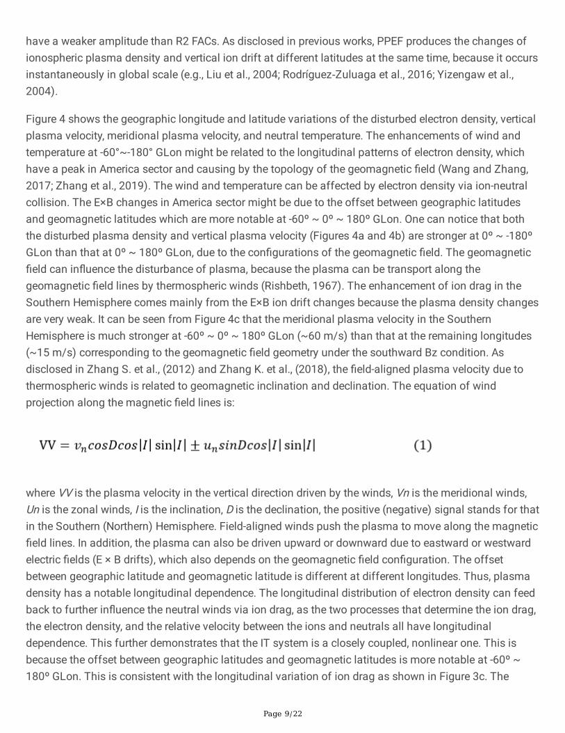
Figure 4 shows the geographic longitude and latitude variations of the disturbed electron density, verticalplasma velocity, meridional plasma velocity, and neutral temperature. The enhancements of wind andtemperature at -60°~-180° GLon might be related to the longitudinal patterns of electron density, whichhave a peak in America sector and causing by the topology of the geomagnetic �eld (Wang and Zhang,2017; Zhang et al., 2019). The wind and temperature can be affected by electron density via ion-neutralcollision. The E×B changes in America sector might be due to the offset between geographic latitudesand geomagnetic latitudes which are more notable at -60º ~ 0º ~ 180º GLon. One can notice that boththe disturbed plasma density and vertical plasma velocity (Figures 4a and 4b) are stronger at 0º ~ -180ºGLon than that at 0º ~ 180º GLon, due to the con�gurations of the geomagnetic �eld. The geomagnetic�eld can in�uence the disturbance of plasma, because the plasma can be transport along thegeomagnetic �eld lines by thermospheric winds (Rishbeth, 1967). The enhancement of ion drag in theSouthern Hemisphere comes mainly from the E×B ion drift changes because the plasma density changesare very weak. It can be seen from Figure 4c that the meridional plasma velocity in the SouthernHemisphere is much stronger at -60º ~ 0º ~ 180º GLon (~60 m/s) than that at the remaining longitudes(~15 m/s) corresponding to the geomagnetic �eld geometry under the southward Bz condition. Asdisclosed in Zhang S. et al., (2012) and Zhang K. et al., (2018), the �eld-aligned plasma velocity due tothermospheric winds is related to geomagnetic inclination and declination. The equation of windprojection along the magnetic �eld lines is:

where VV is the plasma velocity in the vertical direction driven by the winds, Vn is the meridional winds,Un is the zonal winds, I is the inclination, D is the declination, the positive (negative) signal stands for thatin the Southern (Northern) Hemisphere. Field-aligned winds push the plasma to move along the magnetic�eld lines. In addition, the plasma can also be driven upward or downward due to eastward or westwardelectric �elds (E × B drifts), which also depends on the geomagnetic �eld con�guration. The offsetbetween geographic latitude and geomagnetic latitude is different at different longitudes. Thus, plasmadensity has a notable longitudinal dependence. The longitudinal distribution of electron density can feedback to further in�uence the neutral winds via ion drag, as the two processes that determine the ion drag,the electron density, and the relative velocity between the ions and neutrals all have longitudinaldependence. This further demonstrates that the IT system is a closely coupled, nonlinear one. This isbecause the offset between geographic latitudes and geomagnetic latitudes is more notable at -60º ~180º GLon. This is consistent with the longitudinal variation of ion drag as shown in Figure 3c. The

Page 10/22

longitudinal variation of the ion drag related to the E×B drift can explain the longitudinal variation of thebroken mean circulation. 

There also exists a signi�cant hemispheric asymmetry in the broken mean circulation, caused by thecombined roles of pressure gradient and ion drag. In the longitude sector (-60º ~ 0º ~ 180º GLon), boththe effects of pressure gradient and ion drag are strong enough and cannot overwhelm each other in theSouthern Hemisphere. As shown in Figure 4a, the electron density enhancements are more than 3 × 1011

m-3 at geomagnetic latitudes above 20º MLat in the Northern Hemisphere, which are signi�cantlystronger than those in the Southern Hemisphere (1 × 1011 m-3). Thus, the ion drag effects, which areproportional to the plasma density, show the corresponding patterns. In addition, the plasma densitychanges in the Northern Hemisphere are much larger at 0º ~ -180º GLon (~5 × 1011 m-3) than those at 0º~ 180º GLon (~3 × 1011 m-3), thus the ion drag effects are also stronger in the 0º ~ -180º GLon sector.Note here that in Figure 3b, the pressure gradient that is associated with temperature disturbances underthe temporal oscillations of IMF Bz conditions has similar magnitudes in the two hemispheres, and doesnot show outstanding longitudinal patterns as that in the ion drag effects. Then, the role of ion dragoverpowers the pressure gradient at this sector and is overwhelmed at the remaining longitudes. 

Standing signature

As shown in Figure 2c, the TADs of meridional winds stand at ~20º MLat. A similar standing feature canbe found in the plasma density (Figure 4a) and neutral temperature (Figure 4d). As shown in Figure 3, thestanding feature in the meridional wind is due to the combined roles of ion drag and pressure gradient.

As disclosed in the literature (e.g., Breig, 1987; Fejer et al., 1999), the E×B drifts, ambipolar diffusion,thermospheric neutral winds, and chemistry are vital in the variations of ionospheric electron density atmiddle and low latitudes. Daytime PPEF is eastward for the undershielding and westward for theovershielding (Peymirat et al., 2000). Then, the ionospheric plasma is driven upward/downward along thedirection transverse to the magnetic �eld line, causing the density enhancement/decrease that isdependent on the longitudes in the LT-�xed map, as shown in Figure 4a. The plasma density enhances atalmost all longitudes at ~20º MLat (black curve line, Figure 4a) in the Northern Hemisphere. This couldbe related to the standing feature of TADs (Figure 2c). The density enhances signi�cantly at MLat above20º MLat, introducing strong ion drag effects to the equatorward propagation TADs in meridional winds.Thus, the meridional winds are slowed down in this sector, with a pattern of standing feature. The plasmamoves to high altitudes at the equator, then decrease to low altitudes along the magnetic �eld line for theambipolar diffusion, summer-winter thermospheric winds, and gravity force, producing the notableequatorial ion anomaly (EIA) structures that are signi�cant at ~20º MLat (black curve line, Figure 4a). At~20º MLat, the density changes are stronger at 120º ~ 300º GLon (120º ~ 180º and -180º ~ -60º) thanthose at remaining longitudes due to the geomagnetic �eld topology, consistent with the results of Immeland Mannucci (2013) and Greer and Ridley (2017). Because ionospheric plasma can move along thegeomagnetic �eld lines by ambipolar diffusion and neutral winds. The plasma can also be transportedupward/downward under the effects of eastward/westward electric �elds (E×B drifts). The

Page 11/22

equatorward/poleward winds can move the plasma along the magnetic �eld lines (upward/downward)due to the wind projection as shown in equation (1), producing density changes. The transportation ofplasma due to the winds has a close relationship with the geomagnetic con�guration. For instance, whenthe declination is negative (positive), the eastward winds can move the plasma to a higher (lower)altitude, causing an enhancement (decrease) of electron density. In the Northern (Southern) Hemisphere,there are two (one) zones of negative declination and two (one) zones of positive declination. Thus, theelectron densities with the modi�cation of geomagnetic �eld morphology can have large longitudinalvariations. Thus, the effects of ion drag overpower the pressure gradient and prevent the propagating ofTADs at 120º ~ 300º GLon (120º ~ 180º and -180º ~ -60º), which is a key factor in the standing featurein meridional winds at these longitudes. 

At -60º ~ 120º GLon, the effect of the pressure gradient on the meridional wind dominates over the iondrag when the electron density is weak (Figure 3a). Note here that the temperature seems to be enhancedmore at latitudes above 20º MLat than that at 0º ~ 20º MLat, indicated by the black curve line (Figure4d). Thus, the standing feature at this longitudinal sector seems to be related to the neutral temperaturechanges, which exhibit a similar structure. At this longitude sector, the offset between the geomagneticand geographic latitudes is more notable, correspondingly the neutral temperature change can be larger.Because the electron density changes are noticeable in this longitude sector, and thus the correspondingneutral temperature change due to the plasma collisional heating, which is the dominant heatingmechanism for the neutrals in the upper thermosphere, is large (Zhang et al., 2018). 

In addition, the standing feature appears only in the Northern Hemisphere, showing a signi�canthemispheric asymmetry. This asymmetry is closely related to the electron density changes under thetemporal oscillations of IMF Bz conditions. At ~300 km, the electron density (Figure 4a) changes aremuch larger in the Northern Hemisphere than those in the opposite hemisphere, owing to the meridionalwind transportation. In Figure 2c, the meridional wind changes are equatorward at MLat above 20º, andnorthward at MLat less than 20º. The equatorward winds can transfer plasma from high to low latitudesalong the magnetic �eld lines, whereas, the northward winds at low latitudes can push plasma fromSouthern to Northern Hemisphere. The density changes in the Northern Hemisphere are greater than 3 ×1011 m-3 at geomagnetic latitudes along and above 20º MLat, whereas those are ~1 × 1011 m-3 at theconjugated latitudes in the Southern Hemisphere. The stronger the plasma density changes are, the largerin�uences of ion drag on the meridional winds are (Figures 3a and 3c). Thus, the equatorwardpropagation of TADs in the Northern Hemisphere stands at ~20º MLat, and does not appear in theSouthern Hemisphere.

ConclusionUsing coupled magnetosphere-thermosphere-ionosphere model results, the hemispheric and longitudinaldifferences of the meridional wind changes during oscillating interplanetary magnetic �eld Bz at 60-minare explored in this work. The main results are shown below.

Page 12/22

1) The broken mean circulation only exists at 0º~180º geographic longitude (GLon) in the SouthernHemisphere, which is due to the combined roles of the pressure gradient and ion drag forces.

2) The standing features in TADs of meridional winds are found at ~20º magnetic latitude (MLat), whichare induced by the geomagnetic �eld con�gurations, neutral temperature, and electron density changes.

List Of AbbreviationsInterplanetary magnetic �eld (IMF).

Magnetic latitude (MLat).

Travelling atmospheric disturbances (TADs).

Ionosphere-Thermosphere (IT).

Traveling ionospheric disturbances (TID).

CHAllenging Minisatellite Payload (CHAMP).

Coupled Magnetosphere Ionosphere Thermosphere (CMIT).

Thermosphere Ionosphere Electrodynamic General Circulation Model (TIEGCM).

Lyon–Fedder–Mobarry (LFM).

Geographic latitudes (GLat).

Geographic longitude (GLon).

Region 1 (R1).

Region 2 (R2).

Field-aligned currents (FACs).

Equatorial ion anomaly (EIA).

DeclarationsAvailability of data and materials

The IMF data comes from OMNI website (https://omniweb.gsfc.

nasa.gov/). The CHAMP thermospheric data is from the website (ftp://isdcftp.gfz-potsdam.de/champ/).The CHAMP neutral density can be downloaded from the website (http://thermosphere.tudelft.nl/). The

Page 13/22

model outputs are stored in the NCAR High Performance Storage System(https://www2.cisl.ucar.edu/resources/storage-and-�le-systems/hpss).

Competing interest

  The authors declare that they have no competing interests.

Funding

  The National Center for Atmospheric Research is sponsored by the National Science Foundation. We arereally grateful for the sponsor from the National Nature Science Foundation of China (NO. 41974182,41674153, 41431073, 41521062 and 42004135), and the Spark Project at Wuhan University(2042020gf0024).

Authors' contributions

Kedeng Zhang, Hui Wang, Wenbin Wang, Jing Liu made contributes to the theoretic interpretation ofresults and drafted the manuscript. Kedeng Zhang and Jie Gao made contributions on the dataprocessing and model work. 

          Acknowledgments

             The operational support of the CHAMP mission by the German Aerospace Center (DLR) aregratefully acknowledged. 

ReferencesBlanc, M., & Richmond, A. D. (1980). The ionospheric disturbance dynamo. Journal of GeophysicalResearch: Space Physics, 85(A4), 1669-1686.

Breig, E. L. (1987). Thermospheric ion and neutral composition and chemistry. Reviews of Geophysics,25(3), 455-470.

Bruinsma, S. L., & Forbes, J. M. (2007). Global observation of traveling atmospheric disturbances (TADs)in the thermosphere. Geophysical Research Letters, 34(14).

Bruinsma, S. L., & Forbes, J. M. (2009). Properties of traveling atmospheric disturbances (TADs) inferredfrom CHAMP accelerometer observations. Advances in Space Research, 43(3), 369-376.

Cnossen, I., and A.D. Richmond (2012). How changes in the tilt angle of the geomagnetic dipole affect thecoupled magnetosphere-ionosphere-thermosphere system, J. Geophys. Res., 117, A10317, doi:10.1029/2012JA018056.

Doornbos, E. (2012). Thermospheric density and wind determination from satellite dynamics. SpringerScience & Business Media.

Page 14/22

Dungey, J. W. (1961). Interplanetary magnetic �eld and the auroral zones. Physical Review Letters, 6(2),47.

Fejer, B. G., Scherliess, L., & De Paula, E. R. (1999). Effects of the vertical plasma drift velocity on thegeneration and evolution of equatorial spread F. Journal of Geophysical Research: Space Physics,104(A9), 19859-19869.

Fejer, B. G., Jensen, J. W., & Su, S. Y. (2008). Seasonal and longitudinal dependence of equatorialdisturbance vertical plasma drifts. Geophysical Research Letters, 35(20).

Forbes, J. M., G. Lu, S. Bruinsma, S. Nerem, and X. Zhang (2005), Thermosphere density variations due tothe 15–24 April 2002 solar events from CHAMP/STAR accelerometer measurements, J. Geophys. Res.,110, A12S27, doi:10.1029/2004JA010856.

Greer, K. R., Immel, T., & Ridley, A. (2017). On the variation in the ionospheric response to geomagneticstorms with time of onset. Journal of Geophysical Research: Space Physics, 122(4), 4512-4525.

Hagan, M. E., and Forbes, J. M. (2002). Migrating and nonmigrating diurnal tides in the middle and upperatmosphere excited by tropospheric latent heat release. Journal of Geophysical Research: Atmospheres,107(D24).

Hagan, M. E., & Forbes, J. M. (2003). Migrating and nonmigrating semidiurnal tides in the upperatmosphere excited by tropospheric latent heat release. Journal of Geophysical Research: Space Physics,108(A2).

Häusler, K., Lühr, H., Rentz, S., and Köhler, W. (2007). A statistical analysis of longitudinal dependences ofupper thermospheric zonal winds at dip equator latitudes derived from CHAMP. Journal of atmosphericand solar-terrestrial physics, 69(12), 1419-1430.

Häusler, K., and Lühr, H. (2009). Nonmigrating tidal signals in the upper thermospheric zonal wind atequatorial latitudes as observed by CHAMP. Ann. Geophys, 27(7), 2643-2652.

Häusler, K., Lühr, H., Hagan, M. E., Maute, A., and Roble, R. G. (2010). Comparison of CHAMP and TIME‐GCM nonmigrating tidal signals in the thermospheric zonal wind. Journal of Geophysical Research:Atmospheres, 115(D1).

Heelis, R. A., Lowell, J. K., and Spiro, R. W. (1982). A model of the high‐latitude ionospheric convectionpattern. Journal of Geophysical Research: Space Physics, 87(A8), 6339-6345.

Hsu, V. W.,J.P.Thayer, W. Wang,and A. Burns (2016), New insights into the complex interplay between dragforces and its thermospheric consequences, J. Geophys. Res. Space Physics, 121, 10,417–10,430,doi:10.1002/2016JA023058.

Page 15/22

Immel, T. J., and A. J. Mannucci (2013), Ionospheric redistribution during geomagnetic storms, J.Geophys. Res. Space Physics, 118, 7928–7939, doi:10.1002/2013JA018919.

Lei, J., Wang, W., Burns, A. G., Solomon, S. C., Richmond, A. D., Wiltberger, M., ... & Reinisch, B. W. (2008).Observations and simulations of the ionospheric and thermospheric response to the December 2006geomagnetic storm: Initial phase. Journal of Geophysical Research: Space Physics, 113(A1).

Li, G., Ning, B., Hu, L., Liu, L., Yue, X., Wan, W., ... & Xu, J. S. (2010). Longitudinal development of low‐latitude ionospheric irregularities during the geomagnetic storms of July 2004. Journal of GeophysicalResearch: Space Physics, 115(A4).

Liu, H., and H. Lühr (2005), Strong disturbance of the upper thermospheric density due to magneticstorms: CHAMP observations, J. Geophys. Res., 110, A09S29, doi:10.1029/2004JA010908.

Liu, J., Zhao, B., & Liu, L. (2010, March). Time delay and duration of ionospheric total electron contentresponses to geomagnetic disturbances. Annales Geophysicae (09927689) 28, no. 3 (2010).

Liu, J., Liu, L., Nakamura, T., Zhao, B., Ning, B., & Yoshikawa, A. (2014). A case study of ionospheric stormeffects during long‐lasting southward IMF Bz‐driven geomagnetic storm. Journal of GeophysicalResearch: Space Physics, 119(9), 7716-7731.

Liu, J., Wang, W., Zhang, B., Huang, C., & Lin, D. (2018a). Temporal Variation of Solar Wind in ControllingSolar Wind‐Magnetosphere‐Ionosphere Energy Budget. Journal of Geophysical Research: Space Physics,123(7), 5862-5869.

Liu, J., Wang, W., Burns, A., Oppenheim, M., & Dimant, Y. (2018b). Faster traveling atmospheredisturbances caused by polar ionosphere turbulence heating. Journal of Geophysical Research: SpacePhysics, 123(3), 2181-2191.

Lyon, J. G., Fedder, J. A., & Mobarry, C. M. (2004). The Lyon–Fedder–Mobarry (LFM) global MHDmagnetospheric simulation code. Journal of Atmospheric and Solar-Terrestrial Physics, 66(15), 1333-1350.

Maute, A., Richmond, A. D., & Roble, R. G. (2012). Sources of low-latitude ionospheric E × B drifts and theirvariability. Journal of Geophysical Research, 117, A06312. https://doi.org/10.1029/2011JA017502

Merkin, V. G., Milikh, G., Papadopoulos, K., Lyon, J., Dimant, Y. S., Sharma, A. S., ... & Wiltberger, M. (2005).Effect of anomalous electron heating on the transpolar potential in the LFM global MHDmodel. Geophysical research letters, 32(22).

Nishida, A. (1968). Coherence of geomagnetic DP 2 �uctuations with interplanetary magnetic variations.Journal of Geophysical Research, 73(17), 5549-5559.

Page 16/22

Oberheide, J., Forbes, J. M., Häusler, K., Wu, Q., and Bruinsma, S. L. (2009). Tropospheric tides from 80 to400 km: Propagation, interannual variability, and solar cycle effects. Journal of Geophysical Research:Atmospheres, 114(D1).

Oliveira, D. M., Zesta, E., Schuck, P. W., & Sutton, E. K. (2017). Thermosphere global time response togeomagnetic storms caused by coronal mass ejections. Journal of Geophysical Research: SpacePhysics, 122, 10,762–10,782. https://doi.org/10.1002/2017JA024006.

Otsuka, Y., Shiokawa, K., Ogawa, T., & Wilkinson, P. (2004). Geomagnetic conjugate observations ofmedium‐scale traveling ionospheric disturbances at midlatitude using all‐sky airglow imagers.Geophysical research letters, 31(15).

Peymirat, C., Richmond, A. D., & Kobea, A. T. (2000). Electrodynamic coupling of high and low latitudes:Simulations of shielding/overshielding effects. Journal of Geophysical Research: Space Physics,105(A10), 22991-23003.

Reigber, C., Lühr, H., and Schwintzer, P. (2002). CHAMP mission status. Advances in Space Research,30(2), 129-134.

Richards, P. G., Fennelly, J. A., and Torr, D. G. (1994). EUVAC: A solar EUV �ux model for aeronomiccalculations. Journal of Geophysical Research: Space Physics, 99(A5), 8981-8992.

Richmond, A. D., Ridley, E. C., and Roble, R. G. (1992). A thermosphere/ionosphere general circulationmodel with coupled electrodynamics. Geophysical Research Letters, 19(6), 601-604.

Richmond, A. D. (1995), Ionospheric electrodynamics, in Handbook of Ionospheric Electrodynamics, vol. II,pp. 249–290, CRC Press, Boca Raton, Fla

Ridley, A. J. (2005). A new formulation for the ionospheric cross polar cap potential including saturationeffects. In Annales Geophysicae (Vol. 23, No. 11, pp. 3533-3547).

Rishbeth, H. (1967). The effect of winds on the ionospheric F2-peak. Journal of Atmospheric andTerrestrial Physics, 29(3), 225–238. https://doi.org/10.1016/0021-9169(67)90192-4.

Rodríguez‐Zuluaga, J., Radicella, S. M., Nava, B., Amory‐Mazaudier, C., Mora‐Páez, H., & Alazo‐Cuartas, K.(2016). Distinct responses of the low‐latitude ionosphere to CME and HSSWS: The role of the IMF Bzoscillation frequency. Journal of Geophysical Research: Space Physics, 121(11).

Sahai, Y., Fagundes, P. R., Becker-Guedes, F., Abalde, J. R., Crowley, G., Pi, X., ... & Bittencourt, J. A. (2004,September). Longitudinal differences observed in the ionospheric F-region during the major geomagneticstorm of 31 March 2001. In Annales Geophysicae (Vol. 22, No. 9, pp. 3221-3229).

Sharma, S., Galav, P., Dashora, N., & Pandey, R. (2011, June). Longitudinal study of the ionosphericresponse to the geomagnetic storm of 15 May 2005 and manifestation of TADs. In Annales Geophysicae

Page 17/22

(Vol. 29, No. 6, pp. 1063-1070). Copernicus GmbH.

Shiokawa, K., Ihara, C., Otsuka, Y., & Ogawa, T. (2003). Statistical study of nighttime medium‐scaletraveling ionospheric disturbances using midlatitude airglow images. Journal of Geophysical Research:Space Physics, 108(A1).

Sutton, E. K., Nerem, R. S., & Forbes, J. M. (2007). Density and winds in the thermosphere deduced fromaccelerometer data. Journal of Spacecraft and Rockets, 44(6), 1210-1219.

Sutton, E. K., Forbes, J. M., & Knipp, D. J. (2009). Rapid response of the thermosphere to variations inJoule heating. Journal of Geophysical Research: Space Physics, 114(A4).

Thome, G. D. (1964). Incoherent scatter observations of traveling ionospheric disturbances. Journal ofGeophysical Research, 69(19), 4047-4049.

Wang, H., and Lühr, H. (2016). Longitudinal variation in zonal winds at subauroral regions: Possiblemechanisms. Journal of Geophysical Research: Space Physics, 121(1), 745-763.

Wang, H., and Zhang, K. (2017). Longitudinal structure in electron density at mid-latitudes: upward-propagating tidal effects. Earth, Planets and Space, 69(1), 11.

Wang, W., Wiltberger, M., Burns, A. G., Solomon, S. C., Killeen, T. L., Maruyama, N., & Lyon, J. G. (2004).Initial results from the coupled magnetosphere–ionosphere–thermosphere model: thermosphere–ionosphere responses. Journal of atmospheric and solar-terrestrial physics, 66(15), 1425-1441.

Wang, W., Lei, J., Burns, A. G., Wiltberger, M., Richmond, A. D., Solomon, S. C., ... & Anderson, D. N. (2008).Ionospheric electric �eld variations during a geomagnetic storm simulated by a coupled magnetosphereionosphere thermosphere (CMIT) model. Geophysical Research Letters, 35(18).

Wei, Y., M. Hong, W. Wan, A. Du, J. Lei, B. Zhao, W. Wang, Z. Ren, and X. Yue (2008), Unusually longlasting multiple penetration of interplanetary electric �eld to equatorial ionosphere under oscillating IMFBz, Geophys. Res. Lett., 35, L02102, doi:10.1029/2007GL032305.

Wiltberger, M., Wang, W., Burns, A. G., Solomon, S. C., Lyon, J. G., & Goodrich, C. C. (2004). Initial resultsfrom the coupled magnetosphere ionosphere thermosphere model: Magnetospheric and ionosphericresponses. Journal of atmospheric and solar-terrestrial physics, 66(15), 1411-1423.

Xiong, C., H. Lühr, and B.G. Fejer (2015), Global features of the disturbance winds during storm timededuced from CHAMP observations, J. Geophys. Res. Space Physics, 120, 5137–5150,doi:10.1002/2015JA021302.

Xiong, C., Lühr, H., & Fejer, B. G. (2016). The response of equatorial electrojet, vertical plasma drift, andthermospheric zonal wind to enhanced solar wind input. Journal of Geophysical Research: SpacePhysics, 121(6), 5653-5663.

Page 18/22

Yizengaw, E., Essex, E. A., & Birsa, R. (2004, September). The Southern Hemisphere and equatorial regionionization response for a 22 September 1999 severe magnetic storm. Annales Geophysicae, 22 (8), 2765-2773.

Zhang, K., Wang, W., Wang, H., Dang, T., Liu, J., & Wu, Q. (2018). The Longitudinal Variations of UpperThermospheric Zonal Winds Observed by the CHAMP Satellite at Low and Midlatitudes. Journal ofGeophysical Research: Space Physics, 123(11), 9652-9668.

Zhang, K., Liu, J., Wang, W., & Wang, H. (2019). The effects of IMF Bz periodic oscillations onthermospheric meridional winds. Journal of Geophysical Research: Space Physics.

Zhang, S.-R., J. C. Foster, J. M. Holt, P. J. Erickson, and A. J. Coster (2012), Magnetic declination and zonalwind effects on longitudinal differences of ionospheric electron density at midlatitudes, J. Geophys. Res.,117, A08329, doi:10.1029/2012JA017954.

Figures

Page 19/22

Figure 1

(a) The universal time (UT) oscillations of IMF Bz on Nov 11, 2003. (b) The geographic latitude variationsof neutral density changes observed by CHAMP satellite on Nov 11, 2003. The background neutraldensity during the quiet time (Nov. 8) has been removed. The average UT for three CHAMP orbits was~03 UT, ~05 UT, and ~06 UT. The local time of the CHAMP orbit is ~12 LT. The magenta arrows show theequatorward propagation of TADs in neutral density. (c) The universal Time changes of neutral densityobserved by CHAMP are the same as that reported in Figure 3 of Liu and Lühr, (2005). The black arrowsoverplotted are the combined effects of the traveling atmospheric disturbances and simultaneous

Page 20/22

responses in neutral density on 29-31 Oct, 2003. (d) The same as Figure 1c, but for the electron densityobserved by CHAMP. The black arrows overplotted are the combined effects of the traveling ionosphericdisturbances and simultaneous responses in electron density on 29-31 Oct, 2003.

Figure 2

The geographic longitude and latitude variations of thermospheric meridional (VN) winds in the basecase (a), in the 60-min case (b), and the wind responses (c) to the temporal oscillations of IMF Bz in the60-min case at 12 LT. The background winds in the CMIT base case have been removed from that in the60-min case to show the wind responses. The red and black lines overplotted are the geomagnetic

Page 21/22

equator and 20º MLAT, respectively. The positive in meridional winds is northward. The speed is given inm/s. The pressure level is 2.875 (~315 km), which is de�ned as ln(P0/P), where P0=5 × 10-5 Pa. The redand black arrows show the equatorward propagation of TADs in meridional winds.

Figure 3

Differences of forcing terms of meridional winds between CMIT 60-min oscillation case and the base run.The top to bottom panels are the acceleration changes due to all forcing, the pressure gradient, and iondrag, respectively. The acceleration is given in cm/s2. The pressure level is 2.875 (~315 km).

Page 22/22

Figure 4

Similar to Figure 2, but for (a) electron density (NE), (b) vertical plasma velocity (WI E×B), (c) meridionalplasma velocity (VI E×B), and (d) neutral temperature (TN) responses. The density is given in 1010 m-3.The plasma velocity is given in m/s. The temperature is given in K. The pressure level is 2.875 (~315 km).

Supplementary Files

This is a list of supplementary �les associated with this preprint. Click to download.

graphicalabstractimage.png