b r a c e - carnegie mellon school of computer...
TRANSCRIPT

Inference and Learning inGM
Eric Xing
Lecture 18, November 10, 2015
Machine Learning
10-701, Fall 2015
Reading: Chap. 8, C.B book
b r a c e
1© Eric Xing @ CMU, 2006-2015

Inference and Learning We now have compact representations of probability
distributions: BN
A BN M describes a unique probability distribution P
Typical tasks:
Task 1: How do we answer queries about P?
We use inference as a name for the process of computing answers to such queries
Task 2: How do we estimate a plausible model M from data D?
i. We use learning as a name for the process of obtaining point estimate of M.
ii. But for Bayesian, they seek p(M |D), which is actually an inference problem.
iii. When not all variables are observable, even computing point estimate of M need to do inference to impute the missing data.
2© Eric Xing @ CMU, 2006-2015

Approaches to inference Exact inference algorithms
The elimination algorithm Belief propagation The junction tree algorithms (but will not cover in detail here)
Approximate inference techniques
Variational algorithms Stochastic simulation / sampling methods Markov chain Monte Carlo methods
3© Eric Xing @ CMU, 2006-2015

A food web:
Query: P(h)
By chain decomposition, we get
Marginalization and Elimination
g f e d c b a
hgfedcbaPhP ),,,,,,,()(
B A
DC
E F
G H
a naïve summation needs to enumerate over an exponential number of terms
What is the probability that hawks are leaving given that the grass condition is poor?
),|()|()|(),|()|()|()()( fehPegPafPdcePadPbcPbPaPg f e d c b a
4© Eric Xing @ CMU, 2006-2015

Query: P(A |h) Need to eliminate: B,C,D,E,F,G,H
Initial factors:
Choose an elimination order: H,G,F,E,D,C,B
Step 1: Conditioning (fix the evidence node (i.e., h) on its observed value (i.e., )):
This step is isomorphic to a marginalization step:
B A
DC
E F
G H
),|()|()|(),|()|()|()()( fehPegPafPdcePadPbcPbPaP
),|~(),( fehhpfemh h~
h
h hhfehpfem )~(),|(),(
B A
DC
E F
G
Variable Elimination
5© Eric Xing @ CMU, 2006-2015

Query: P(B |h) Need to eliminate: B,C,D,E,F,G
Initial factors:
Step 2: Eliminate G compute
B A
DC
E F
G H),()|()|(),|()|()|()()(
),|()|()|(),|()|()|()()(femegPafPdcePadPbcPbPaP
fehPegPafPdcePadPbcPbPaP
h
1)|()( g
g egpemB A
DC
E F),()|(),|()|()|()()(
),()()|(),|()|()|()()(
femafPdcePadPbcPbPaP
fememafPdcePadPbcPbPaP
h
hg
Example: Variable Elimination
6© Eric Xing @ CMU, 2006-2015

Query: P(B |h) Need to eliminate: B,C,D,E,F
Initial factors:
Step 3: Eliminate F compute
B A
DC
E F
G H
Example: Variable Elimination
),()|(),|()|()|()()(),()|()|(),|()|()|()()(
),|()|()|(),|()|()|()()(
femafPdcePadPbcPbPaPfemegPafPdcePadPbcPbPaP
fehPegPafPdcePadPbcPbPaP
h
h
f
hf femafpaem ),()|(),(
),(),|()|()|()()( eamdcePadPbcPbPaP f
B A
DC
E
7© Eric Xing @ CMU, 2006-2015

B A
DC
E
Query: P(B |h) Need to eliminate: B,C,D,E
Initial factors:
Step 4: Eliminate E compute
B A
DC
E F
G H
Example: Variable Elimination
),(),|()|()|()()(),()|(),|()|()|()()(
),()|()|(),|()|()|()()(),|()|()|(),|()|()|()()(
eamdcePadPbcPbPaPfemafPdcePadPbcPbPaP
femegPafPdcePadPbcPbPaPfehPegPafPdcePadPbcPbPaP
f
h
h
e
fe eamdcepdcam ),(),|(),,(
),,()|()|()()( dcamadPbcPbPaP e
B A
DC
8© Eric Xing @ CMU, 2006-2015

Query: P(B |h) Need to eliminate: B,C,D
Initial factors:
Step 5: Eliminate D compute
B A
DC
E F
G H
Example: Variable Elimination
),,()|()|()()(
),(),|()|()|()()(),()|(),|()|()|()()(
),()|()|(),|()|()|()()(),|()|()|(),|()|()|()()(
dcamadPbcPbPaP
eamdcePadPbcPbPaPfemafPdcePadPbcPbPaP
femegPafPdcePadPbcPbPaPfehPegPafPdcePadPbcPbPaP
e
f
h
h
d
ed dcamadpcam ),,()|(),(
),()|()()( camdcPbPaP d
B A
C
9© Eric Xing @ CMU, 2006-2015

Query: P(B |h) Need to eliminate: B,C
Initial factors:
Step 6: Eliminate C compute
B A
DC
E F
G H
Example: Variable Elimination
),()|()()( camdcPbPaP d
c
dc cambcpbam ),()|(),(
),()|()()(),,()|()|()()(
),(),|()|()|()()(),()|(),|()|()|()()(
),()|()|(),|()|()|()()(),|()|()|(),|()|()|()()(
camdcPbPaPdcamadPdcPbPaP
eamdcePadPdcPbPaPfemafPdcePadPdcPbPaP
femegPafPdcePadPdcPbPaPfehPegPafPdcePadPdcPbPaP
d
e
f
h
h
B A
10© Eric Xing @ CMU, 2006-2015

Query: P(B |h) Need to eliminate: B
Initial factors:
Step 7: Eliminate B compute
B A
DC
E F
G H
Example: Variable Elimination
),()()(),()|()()(
),,()|()|()()(
),(),|()|()|()()(),()|(),|()|()|()()(
),()|()|(),|()|()|()()(),|()|()|(),|()|()|()()(
bambPaPcamdcPbPaP
dcamadPdcPbPaP
eamdcePadPdcPbPaPfemafPdcePadPdcPbPaP
femegPafPdcePadPdcPbPaPfehPegPafPdcePadPdcPbPaP
c
d
e
f
h
h
b
cb bambpam ),()()(
)()( amaP b
A
11© Eric Xing @ CMU, 2006-2015

Query: P(B |h) Need to eliminate: B
Initial factors:
Step 8: Wrap-up
B A
DC
E F
G H
Example: Variable Elimination
)()(),()()(
),()|()()(),,()|()|()()(
),(),|()|()|()()(),()|(),|()|()|()()(
),()|()|(),|()|()|()()(),|()|()|(),|()|()|()()(
amaPbambPaP
camdcPbPaPdcamadPdcPbPaP
eamdcePadPdcPbPaPfemafPdcePadPdcPbPaP
femegPafPdcePadPdcPbPaPfehPegPafPdcePadPdcPbPaP
b
c
d
e
f
h
h
, )()()~,( amaphap b
ab
b
amapamaphaP
)()()()()~|(
a
b amaphp )()()~(
12© Eric Xing @ CMU, 2006-2015

Suppose in one elimination step we compute
This requires multiplications
─ For each value of x, y1, …, yk, we do k multiplications
additions
─ For each value of y1, …, yk , we do |Val(X)| additions
Complexity is exponential in number of variables in the intermediate factor
x
kxkx yyxmyym ),,,('),,( 11
k
icikx i
xmyyxm1
1 ),(),,,(' y
i
CiXk )Val()Val( Y
i
CiX )Val()Val( Y
Complexity of variable elimination
13© Eric Xing @ CMU, 2006-2015
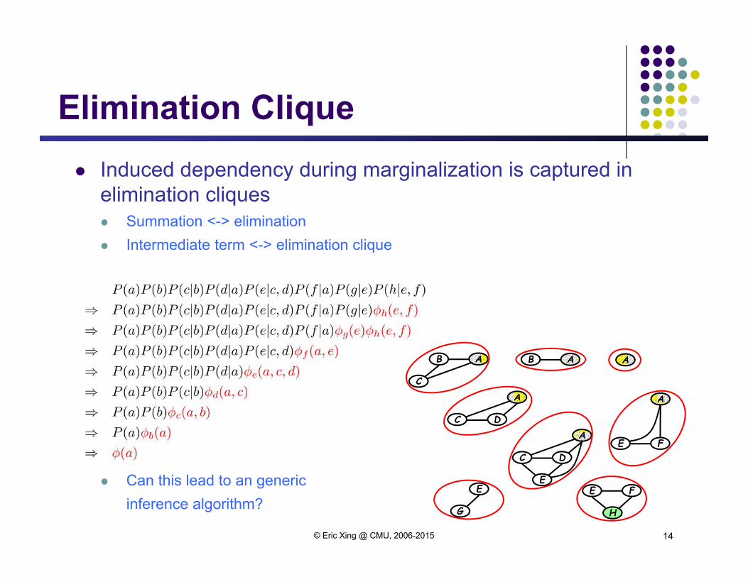
Induced dependency during marginalization is captured in elimination cliques Summation <-> elimination Intermediate term <-> elimination clique
Can this lead to an generic inference algorithm?
Elimination Clique
E F
H
A
E F
B A
C
E
G
A
DC
E
A
DC
B A A
14© Eric Xing @ CMU, 2006-2015

Elimination message passing on a clique tree
Messages can be reused
E F
H
A
E F
B A
C
E
G
A
DC
E
A
DC
B A A
hmgm
emfm
bmcm
dm
From Elimination to Message Passing
e
fg
e
eamemdcepdcam
),()(),|(),,(
15© Eric Xing @ CMU, 2006-2015

E F
H
A
E F
B A
C
E
G
A
DC
E
A
DC
B A A
cm bm
gm
em
dmfm
hm
From Elimination to Message Passing
Elimination message passing on a clique tree Another query ...
Messages mf and mh are reused, others need to be recomputed
16© Eric Xing @ CMU, 2006-2015

From elimination to message passing Recall ELIMINATION algorithm:
Choose an ordering Z in which query node f is the final node Place all potentials on an active list Eliminate node i by removing all potentials containing i, take sum/product over xi. Place the resultant factor back on the list
For a TREE graph: Choose query node f as the root of the tree View tree as a directed tree with edges pointing towards from f Elimination ordering based on depth-first traversal Elimination of each node can be considered as
message-passing (or Belief Propagation) directly along tree branches, rather than on some transformed graphs
thus, we can use the tree itself as a data-structure to do general inference!!
17© Eric Xing @ CMU, 2006-2015

f
i
j
k l
Message passing for trees
Let mij(xi) denote the factor resulting from eliminating variables from bellow up to i, which is a function of xi:
This is reminiscent of a message sent from j to i.
mij(xi) represents a "belief" of xi from xj!
18© Eric Xing @ CMU, 2006-2015

Elimination on trees is equivalent to message passing along tree branches!
f
i
j
k l19© Eric Xing @ CMU, 2006-2015

m24(X 4)
X1
X2
X3X4
The message passing protocol: A two-pass algorithm:
m21(X 1)
m32(X 2) m42(X 2)
m12(X 2)
m23(X 3)20© Eric Xing @ CMU, 2006-2015

Belief Propagation (SP-algorithm): Sequential implementation
21© Eric Xing @ CMU, 2006-2015

Inference on general GM Now, what if the GM is not a tree-like graph?
Can we still directly run message message-passing protocol along its edges?
For non-trees, we do not have the guarantee that message-passing will be consistent!
Then what? Construct a graph data-structure from P that has a tree structure, and run message-passing
on it!
Junction tree algorithm
22© Eric Xing @ CMU, 2006-2015

Summary: Exact Inference The simple Eliminate algorithm captures the key algorithmic
Operation underlying probabilistic inference:--- That of taking a sum over product of potential functions
The computational complexity of the Eliminate algorithm can be reduced to purely graph-theoretic considerations.
This graph interpretation will also provide hints about how to design improved inference algorithms
What can we say about the overall computational complexity of the algorithm? In particular, how can we control the "size" of the summands that appear in the sequence of summation operation.
23© Eric Xing @ CMU, 2006-2015

Approaches to inference Exact inference algorithms
The elimination algorithm Belief propagation The junction tree algorithms (but will not cover in detail here)
Approximate inference techniques
Variational algorithms Stochastic simulation / sampling methods Markov chain Monte Carlo methods
24© Eric Xing @ CMU, 2006-2015

Monte Carlo methods Draw random samples from the desired distribution
Yield a stochastic representation of a complex distribution marginals and other expections can be approximated using sample-based
averages
Asymptotically exact and easy to apply to arbitrary models
Challenges: how to draw samples from a given dist. (not all distributions can be trivially
sampled)?
how to make better use of the samples (not all sample are useful, or eqally useful, see an example later)?
how to know we've sampled enough?
© Eric Xing @ CMU, 2006-2015
N
t
txfN
xf1
1 )()]([ )(E

Example: naive sampling Construct samples according to probabilities given in a BN.
© Eric Xing @ CMU, 2006-2015
Alarm example: (Choose the right sampling sequence)1) Sampling:P(B)=<0.001, 0.999> suppose it is false, B0. Same for E0. P(A|B0, E0)=<0.001, 0.999> suppose it is false... 2) Frequency counting: In the samples right, P(J|A0)=P(J,A0)/P(A0)=<1/9, 8/9>.
E0 B0 A0 M0 J0
E0 B0 A0 M0 J0
E0 B0 A0 M0 J1
E0 B0 A0 M0 J0
E0 B0 A0 M0 J0
E0 B0 A0 M0 J0
E1 B0 A1 M1 J1
E0 B0 A0 M0 J0
E0 B0 A0 M0 J0
E0 B0 A0 M0 J0
E0 B0 A0 M0 J0
E0 B0 A0 M0 J0
E0 B0 A0 M0 J1
E0 B0 A0 M0 J0
E0 B0 A0 M0 J0
E0 B0 A0 M0 J0
E1 B0 A1 M1 J1
E0 B0 A0 M0 J0
E0 B0 A0 M0 J0
E0 B0 A0 M0 J0

Example: naive sampling Construct samples according to probabilities given in a BN.
© Eric Xing @ CMU, 2006-2015
Alarm example: (Choose the right sampling sequence)
3) what if we want to compute P(J|A1) ? we have only one sample ...P(J|A1)=P(J,A1)/P(A1)=<0, 1>.
4) what if we want to compute P(J|B1) ? No such sample available!P(J|A1)=P(J,B1)/P(B1) can not be defined.
For a model with hundreds or more variables, rare events will be very hard to garner evough samples even after a long time or sampling ...
E0 B0 A0 M0 J0
E0 B0 A0 M0 J0
E0 B0 A0 M0 J1
E0 B0 A0 M0 J0
E0 B0 A0 M0 J0
E0 B0 A0 M0 J0
E1 B0 A1 M1 J1
E0 B0 A0 M0 J0
E0 B0 A0 M0 J0
E0 B0 A0 M0 J0

Markov chain Monte Carlo (MCMC) Construct a Markov chain whose stationary distribution is the
target density = P(X|e). Run for T samples (burn-in time) until the chain
converges/mixes/reaches stationary distribution. Then collect M (correlated) samples xm . Key issues:
Designing proposals so that the chain mixes rapidly. Diagnosing convergence.
© Eric Xing @ CMU, 2006-2015

Markov Chains Definition:
Given an n-dimensional state space Random vector X = (x1,…,xn) x(t) = x at time-step t x(t) transitions to x(t+1) with prob
P(x(t+1) | x(t),…,x(1)) = T(x(t+1) | x(t)) = T(x(t) x(t+1))
Homogenous: chain determined by state x(0), fixed transition kernel Q (rows sum to 1)
Equilibrium: (x) is a stationary (equilibrium) distribution if (x') = x(x) Q(xx').
i.e., is a left eigenvector of the transition matrix T = TQ.
© Eric Xing @ CMU, 2006-2015
05050307007500250
305020305020..
....
......X1 X2
X3
0.25 0.7
0.50.50.75 0.3

Gibbs sampling The transition matrix updates each node one at a time using
the following proposal:
It is efficient since only depends on the values in Xi’s Markov blanket
© Eric Xing @ CMU, 2006-2015
)|'(),'(),( iiiiii xpxx xxxQ
)|( 'iixp x

Gibbs sampling Gibbs sampling is an MCMC algorithm that is especially
appropriate for inference in graphical models.
The procedue we have variable set X={x1, x2, x3,... xN} for a GM
at each step one of the variables Xi is selected (at random or according to some fixed sequences), denote the remaining variables as X-i , and its current value as x-i
(t-1)
Using the "alarm network" as an example, say at time t we choose XE, and we denote the current value assignments of the remaining variables, X-E , obtained from previous samples, as
the conditonal distribution p(Xi| x-i(t-1)) is computed
a value xi(t) is sampled from this distribution
the sample xi(t) replaces the previous sampled value of Xi in X.
i.e., © Eric Xing @ CMU, 2006-2015
)()()()()( ,,, 11111 t
Mt
Jt
At
BtE xxxxx
)()()( tE
tE
t xxx
1

Markov Blanket
© Eric Xing @ CMU, 2006-2015
Markov Blanket in BN A variable is independent from
others, given its parents, children and children‘s parents (d-separation).
MB in MRF A variable is independent all its
non-neighbors, given all its direct neighbors.
p(Xi| X-i)= p(Xi| MB(Xi))
Gibbs sampling Every step, choose one variable
and sample it by P(X|MB(X)) based on previous sample.

Gibbs sampling of the alarm network
© Eric Xing @ CMU, 2006-2015
To calculate P(J|B1,M1) Choose (B1,E0,A1,M1,J1) as a
start Evidences are B1, M1, variables
are A, E, J. Choose next variable as A Sample A by
P(A|MB(A))=P(A|B1, E0, M1, J1) suppose to be false.
(B1, E0, A0, M1, J1) Choose next random variable
as E, sample E~P(E|B1,A0) ...MB(A)={B, E, J, M}
MB(E)={A, B}

Example
© Eric Xing @ CMU, 2006-2015

Example:
© Eric Xing @ CMU, 2006-2015

Example
© Eric Xing @ CMU, 2006-2015

ExampleP(J1 | B1,M1) = 0.90P(J1 | E1,M0) = 0.14P(E1 | J1) = 0.01P(E1 | M1) = 0.04P(E1 | M1,J1) = 0.17
© Eric Xing @ CMU, 2006-2015

The of simulation Run several chains Start at over-dispersed
points Monitor the log lik. Monitor the serial
correlations Monitor acceptance ratios
Re-parameterize (to get approx. indep.)
Re-block (Gibbs) Collapse (int. over other
pars.) Run with troubled pars.
fixed at reasonable vals.
© Eric Xing @ CMU, 2006-2015

The goal:
Given set of independent samples (assignments of random variables), find the best (the most likely?) Bayesian Network (both DAG and CPDs)
(B,E,A,C,R)=(T,F,F,T,F)(B,E,A,C,R)=(T,F,T,T,F)……..
(B,E,A,C,R)=(F,T,T,T,F)
E
R
B
A
C
0.9 0.1
e
be
0.2 0.8
0.01 0.990.9 0.1
bebb
e
BE P(A | E,B)
E
R
B
A
C
Learning Graphical Models
39© Eric Xing @ CMU, 2006-2015

Learning Graphical Models (cont.) Scenarios:
completely observed GMs directed undirected
partially observed GMs directed undirected (an open research topic)
Estimation principles: Maximal likelihood estimation (MLE) Bayesian estimation Maximal conditional likelihood Maximal "Margin"
We use learning as a name for the process of estimating the parameters, and in some cases, the topology of the network, from data.
40© Eric Xing @ CMU, 2006-2015

MLE for general BN parameters If we assume the parameters for each CPD are globally
independent, and all nodes are fully observed, then the log-likelihood function decomposes into a sum of local terms, one per node:
i ninin
n iinin ii
xpxpDpD ),|(log),|(log)|(log);( ,,,, xxl
X2=1
X2=0
X5=0
X5=1
41© Eric Xing @ CMU, 2006-2015

Consider the distribution defined by the directed acyclic GM:
This is exactly like learning four separate small BNs, each of which consists of a node and its parents.
Example: decomposable likelihood of a directed model
),,|(),|(),|()|()|( 432431321211 xxxpxxpxxpxpxp
X1
X4
X2 X3
X4
X2 X3
X1X1
X2
X1
X3
42© Eric Xing @ CMU, 2006-2015

E.g.: MLE for BNs with tabular CPDs Assume each CPD is represented as a table (multinomial)
where
Note that in case of multiple parents, will have a composite state, and the CPD will be a high-dimensional table
The sufficient statistics are counts of family configurations
The log-likelihood is
Using a Lagrange multiplier to enforce , we get:
)|(def
kXjXpiiijk
iX
nkn
jinijk ixxn ,,
def
kji
ijkijkkji
nijk nD ijk
,,,,
loglog);( l
1j ijk
kjikij
ijkMLijk n
n
,','
43© Eric Xing @ CMU, 2006-2015

Definition of HMM Transition probabilities between
any two states
or
Start probabilities
Emission probabilities associated with each state
or in general:
A AA Ax2 x3x1 xT
y2 y3y1 yT...
... ,)|( , jiit
jt ayyp 11 1
.,,,,lMultinomia~)|( ,,, I iaaayyp Miiiitt 211 1
.,,,lMultinomia~)( Myp 211
.,,,,lMultinomia~)|( ,,, I ibbbyxp Kiiiitt 211
.,|f~)|( I iyxp iitt 1
44© Eric Xing @ CMU, 2006-2015

Supervised ML estimation Given x = x1…xN for which the true state path y = y1…yN is
known,
Define:Aij = # times state transition ij occurs in yBik = # times state i in y emits k in x
We can show that the maximum likelihood parameters are:
If y is continuous, we can treat as NTobservations of, e.g., a Gaussian, and apply learning rules for Gaussian …
' ',
,,
)(#)(#
j ij
ij
n
T
titn
jtnn
T
titnML
ij AA
yyy
ijia
2 1
2 1
' ',
,,
)(#)(#
k ik
ik
n
T
titn
ktnn
T
titnML
ik BB
yxy
ikib
1
1
NnTtyx tntn :,::, ,, 11
n
T
ttntn
T
ttntnn xxpyypypp
1,,
21,,1, )|()|()(log),(log),;( yxyxθl
45© Eric Xing @ CMU, 2006-2015

Consider the distribution defined by the directed acyclic GM:
Need to compute p(xH|xV) inference
What if some nodes are not observed?
),,|(),|(),|()|()|( 132431311211 xxxpxxpxxpxpxp
X1
X4
X2 X3
46© Eric Xing @ CMU, 2006-2015

MLE for BNs with tabular CPDs Assume each CPD is represented as a table (multinomial)
where
Note that in case of multiple parents, will have a composite state, and the CPD will be a high-dimensional table
The sufficient statistics are counts of family configurations
The log-likelihood is
Using a Lagrange multiplier to enforce , we get:
)|(def
kXjXpiiijk
iX
nkn
jinijk ixxn ,,
def
kji
ijkijkkji
nijk nD ijk
,,,,
loglog);( l
1j ijk
kjikij
ijkMLijk n
n
,','
47© Eric Xing @ CMU, 2006-2015

Summary
A GMM describes a unique probability distribution P
Typical tasks:
Task 1: How do we answer queries about P?
We use inference as a name for the process of computing answers to such queries
Task 2: How do we estimate a plausible model M from data D?
i. We use learning as a name for the process of obtaining point estimate of M.
ii. But for Bayesian, they seek p(M |D), which is actually an inference problem.
iii. When not all variables are observable, even computing point estimate of M need to do inference to impute the missing data.
48© Eric Xing @ CMU, 2006-2015