axiomatic and economic approaches to international comparisons · 15 axiomatic and economic...
TRANSCRIPT

This PDF is a selection from an out-of-print volume from the National Bureauof Economic Research
Volume Title: International and Interarea Comparisons of Income, Output,and Prices
Volume Author/Editor: Alan Heston and Robert E. Lipsey, editors
Volume Publisher: University of Chicago Press
Volume ISBN: 0-226-33110-5
Volume URL: http://www.nber.org/books/hest99-1
Publication Date: January 1999
Chapter Title: Axiomatic and Economic Approaches to International Comparisons
Chapter Author: W. Erwin Diewert
Chapter URL: http://www.nber.org/chapters/c8385
Chapter pages in book: (p. 13 - 107)

1 Axiomatic and Economic Approaches to International Comparisons W. Erwin Diewert
For a variety of reasons, it is useful to be able to make accurate comparisons of the relative consumption or real output between countries or between re- gions within a country; for example, aid flows or interregional transfer pay- ments may depend on these multilateral comparisons. Normal bilateral index number theory cannot be applied in this multilateral context because bilateral comparisons are inherently dependent on the choice of a base country and the resulting rankings of countries are not invariant to the choice of the base coun- try. Moreover, it is usually politically unacceptable to have a single country or region play an asymmetrical role in making multilateral comparisons.
The problem of making bilateral index number comparisons has been inten- sively studied for about a century. From the viewpoints of both the economic and the test approaches to bilateral index number theory, a consensus has emerged that the Fisher (1922) ideal price and quantity indexes are probably the best functional forms for index number formulas (see Diewert 1992; and Balk 1995a).’ However, there is no comparable consensus on what is the ap- propriate method for making symmetric multilateral index number compari- sons, that is, comparisons that do not depend on the asymmetrical choice of a base country. Part of the reason for this lack of consensus is that the test or axiomatic approach to multilateral index number theory is not as well devel-
W. Erwin Diewert is professor of economics at the University of British Columbia and a re- search associate of the National Bureau of Economic Research.
This research was supported by a SSHRC grant. The author thanks Bert Balk, Irwin Collier, and Alice Nakamura for helpful suggestions and Tina Corsi for typing a difficult manuscript.
1 . Balk (1995a, 87) argues that the Fisher and the Sat0 (1976)-Vartia (1974,1976) price indexes are both the best from the viewpoint of the test or axiomatic approach to index number theory. However, the Sato-Vartia price and quantity indexes are not superlative and hence are not “best” from the perspective of the economic approach. In addition, Reinsdorf and Dorfman (1995) have shown that the Sato-Vartia indexes do not satisfy the monotonicity axioms that the Fisher in- dexes satisfy.
13

14 W. Erwin Diewert
oped as the bilateral theory. In the last decade, Diewert (1986, 1988), Balk (1989, 1996), and Armstrong (1995) have made a start on developing axiom- atic approaches to multilateral comparisons.* In section 1.1 below, the present paper draws on this literature by suggesting a list of twelve desirable properties or tests for multilateral methods. In sections 1.3-1.12, I evaluate ten different multilateral methods from the perspective of this test approach to multilateral comparisons. I find that none of these methods satisfies all the suggested tests. Thus, it is necessary to make choices about the relative importance of the vari- ous tests.
In section 1.2 below, I suggest a multilateral generalization of the economic approach to making bilateral comparisons. In analogy to the bilateral case (see Diewert 1976), I say that a multilateral system is superlative if it is exact for a flexible linearly homogeneous aggregator function. In sections 1.3-1.12, I de- termine whether the ten multilateral methods studied in this paper are also su- perlative.
Section 1.13 discusses some of the trade-offs between the various methods, and section 1.14 concludes.
Appendix A contains proofs of various propositions, and appendix B tables numerical results for the ten multilateral methods for a three-country, two-com- modity artificial data set.
1.1 Multilateral Axioms or Tests
Suppose that the outputs, inputs, or real consumption expenditures of K countries3 in a bloc of countries are to be compared. Suppose also that there are N homogeneous commodities consumed (or produced) in the K countries during the time periods under consideration and that the price and quantity of commodity n in country k are p f > 0 and y t 2 0, respectively, for n = 1, . . . , N and k = 1, . . . , K.4 Denote the country k price and quantity vector by p = [p:, . . . , p i ] T >> 0, and y k = b:, . . . , y i I r > ON, respectively.s I assume that
2. The study of symmetric multilateral indexes dates back to Walsh (1901, 398-431), Fisher (1922, 297-308), and Gini (1924, 1931). Early research suggesting desirable properties or tests for multilateral indexes includes Drechsler (1973, 18-21), Gerardi (1982, 395-98). Hill (1982, 50), and Hill (1984, 130-32).
3. The “countries” could be different regions or producer establishments. The list of commodi- ties consumed (or produced) by the “countries” must be the same.
4. I interpret yk as the total amount of commodity n consumed (or produced) in country k during the relevant time period and p i as the corresponding average price or unit value. If commodity n is not consumed (or produced) in country k during the period under consideration, then p : > 0 is interpreted as the Hicksian (1940, 114) reservation price that would just induce the consumer to purchase zero units of good n (or just induce the producer to supply zero units of good n). This is the convention on the positivity of prices and quantities used by Armstrong (1995).
5 . Notation: y 2 O,(J >> 0,) means that each component of the N-dimensional column vector y is nonnegative (strictly positive), y > 0, means y 2 0, but y # 0,. and p’y = p . y = Cr=’=,pnyn denotes the inner product of the vectors p and y. The transpose of the column vector y is yr.

15 Axiomatic and Economic Approaches to International Comparisons
all prices are positive and are measured in common units and a common num- eraire currency. I also assume that the aggregate bloc quantity vector is strictly positive; that is, Cf=lyk >> 0,. Finally, denote the N X K matrix of country prices by P = [ p ’ , . . . , p”] and the N X K matrix of country quantities by
The share of bloc consumption (or output or input) for country k, Sk, will depend in general on the matrix of prices P and the matrix of quantities Z Thus, Sk will be a function of the components of P and I: say, Sk(P, Y ) for k = 1, . . . , K. I assume that the domain of definition for these functions is the set of strictly positive country price vectors p > > 0, and nonnegative but nonzero quantity vectors y k > 0, for k = 1, . . . , K with CkK_lyk >> 0,. In the remainder of this paper, I shall call a specific set of functions defined on the above domain of definition, {S’(P, Y ) , . . . , SAP, Y ) } , a multilateral system of bloc share functions or a multilateral method for making international comparisons of aggregate quantities.
Y = [ y ’ , . . * , y K ] .
If there are only two units being compared, then define
QW, p 2 , Y ’ , Y ’ ) = W p ’ , p 2 , Y ’ , y2 ) lS ’ (p ’ , p 2 , Y ’ , Y’>
as the ratio of “country” 2’s share of “output” to “country” 1’s share. The re- sulting function Q(pl, p’, y’ , y’) can be interpreted as a bilateral quantity index. I view a multilateral system as a generalization of bilateral index number the- ory to cover the situation where the number of units being compared is greater than two. In the remainder of this paper, I assume that the number of countries in the bloc is K 2 3 (unless I explicitly assume that K = 2). If there is only one commodity, then there is no index number problem; that is, we will have Sk(P, Y ) = yf/XFl y’, for k = 1, . . . , K . Thus, I also assume that the number of commodities is N 2 2.
In the axiomatic approach to bilateral index number theory (see Walsh 1901, 1921; Fisher 1911, 1922; Eichhorn and Voeller 1976; Diewert 1992, 214-23; Diewert 1993b, 33-34; and Balk 1995a), the function Q(p’, p2, y ’ , y2 ) is hy- pothesized to satisfy various axioms or tests. I shall follow an analogous ap- proach to multilateral index number theory by placing various tests or axioms on the multilateral system of share functions Sk( P, Y ) .
Before I list my multilateral axioms, consider the following example of a multilateral system:
This system of multilateral share functions is the exchange rate system, where country k‘s share of bloc consumption (or output or input) is simply its share of total bloc value and all values are computed using a common numeraire cur- rency.

16 W. Erwin Diewert
I now list twelve desirable properties for multilateral systems. I regard the
The first multilateral axiom is the following:
T1: SHARE TEST: There exist K continuous, positive functions S'fP, Y ) , k = 1, . . . , K, such that C,"_,Sk(P, Y ) = 1 for all P, Y in the domain of definition described above.
first seven properties as being more essential.
It is obvious that share functions must sum to unity. The share test outlined above also added the requirements that each share function be continuous and positive. The test T1 (without the positivity requirement) was proposed in Die- wert (1986, 36) and Diewert (1988,76).
To motivate the second test, suppose that each country's share of bloc output is the same for every commodity, say, p, for country k. Then it seems reason- able to ask that Sk(P, Y ) = p, for each k.
T2: PROPORTIONAL QUANTITIES TEST: Suppose that y k = P,y for k = 1,
This test is a multilateral counterpart to Leontief's (1936) aggregation theorem. The next test is a counterpart to Hicks's (1946, 312-13) aggregation theo-
rem: if each country's price vector pk is proportional to a common positive price vector p , then this p can be used to determine country k's share of bloc output as p * yklZjK=g * yj.
. . . ) Kwith p, > 0 andCf==,P, = 1. Then Sk(P, Y ) = &fork = 1, . . . , K.
T3: PROPORTIONAL PRICES TEST: Suppose that p" = a k p for k = 1, . . . , K with ak > 0 for some p >> 0,. Then Sk(P, Y ) = p * y Vp CjK=,yj for k = 1 , . . . , K.
Thus, if either prices or quantities are proportional across countries, then tests T2 and T3 determine what the country-share functions Sk(P, Y ) must be. The tests T2 and T3 can be interpreted as multilateral counterparts to identity tests for bilateral price and quantity indexes.
The next three tests are invariance or symmetry tests.
OF MEASUREMENT): Let S,, > 0 for n = 1, . . . , N, and let S denpte !he N X N diagonal matrix with the 6, on the main diagonal. Then Sk(SP, 8-lY) = Sk(P, Y ) fork = 1, . . . , K .
The test T4 requires that the system of share functions be invariant to changes in the units of measurement for the N commodities. In the multilateral context, this test was proposed in Diewert (1986,38) and Diewert (1988,78). In the bi- lateral context, this test was proposed in Jevons (1884, 23), Pierson (1896, 131), Fisher (1911,411), andFisher (1922,420).
T4: COMMENSURABILITY TEST (INVARIANCE TO CHANGFS IN THE UNITS
T5: COMMODITY REVERSAL TEST (INVARIANCE TO THE ORDERING OF
COMMODITIES): Let II denote an N X N permutation matrix. Then S' (IIP, I IY) = Sk(P, Y ) for k = 1,. . . , K.

17 Axiomatic and Economic Approaches to International Comparisons
This test implies that a country's share of bloc output remains unchanged if the ordering of the N commodities is unchanged. This test was first proposed in the bilateral context in Fisher (1922,63) and in the multilateral context in Die- wert (1986, 39) and (1988,79).
T6: MULTILATERAL COUNTRY REVERSAL TEST (SYMMETRICAL TREAT- MENT OF COUNTRIES): Let S(P, Y)' = [S'(P, Y ) , . . . , SK(P, Y ) ] denote the row vector of country-share functions, and let II* denote a K X K permuta- tion matrix. Then S(PII*, YII*)' = S(P, Y)TI* .
Thus, if the ordering of the countries is changed or permuted, then the resulting system of share functions is equal to the same permutation of the original share functions. The test T6 means that no country can play an asymmetrical role in the definition of the country-share functions. This property of a multilateral sys- tem was termed base-country invariance by Kravis et al. (1975). When multi- lateral indexes are used by multinational agencies such as the European Union, the OECD, or the World Bank, it is considered vital that the multilateral system satisfy T6. This property can be viewed as a fairness test: each country must be treated in an evenhanded, symmetrical manner.
The next test imposes the requirement that scale differences in the price levels of each country (or the use of different monetary units in each country) do not affect the country shares of bloc output.
T7: MONETARY UNITS TEST: Let ak > 0 for k = 1, . . . , K . Then S k ( a l p l ,
Mathematically, T7 is a homogeneity of degree zero in prices property, a prop- erty that is usually imposed on quantity indexes in bilateral index number the- ory. In the multilateral context, Gerardi (1982, 398), Diewert (1986, 38), and Diewert (1988, 78) proposed this test.
The test T7 is a homogeneity in prices test. The next test is a homogeneity in quantities test.
T8: HOMOGENEITY IN QUANTITIES TEST: For i = 1, . . . , K , Xz > 0, j # i , j = 1, . . . , K , we have S(P, y l , . . . , y'-l, Xy', y'+l, . . . , yK)/SJ(P, y l , . . . ,
. . . , aKpK, Y ) = Sk(p' , . . . , p K , Y ) fork = I , . . . , K.
y1-1, Xty', y'+l, . . . , y") = X,S'(P, Y)/SJ(P, Y ) .
Mathematically, T8 says that the output share of country i relative to country j , SISJ, is linearly homogeneous in the components of the country i quantity vec- tor y ' . This property is usually imposed on bilateral quantity indexes. In the multilateral context, this test was suggested in Gerardi (1982, 397), Diewert (1986, 37), and Diewert (1988,77).
The next test imposes the following very reasonable property: as any com- ponent of country k's quantity vector y k increases, country k's share of bloc out- put should also increase.
T9: MONOTONICITY TEST: Sk(P, y l , . . . , y k , . . . , y " ) is increasing in the components of the vector y k for k = 1, . . . , K .
18 W. Erwin Diewert
Although T9 has not been proposed before in the multilateral context, it has been proposed in the context of bilateral index number theory (see Eichhorn and Voeller 1976,23; and Vogt 1980, 70).
The next two tests can be viewed as consistency in aggregation tests or coun- try-weighting tests.
T10: COUNTRY-PARTITIONING TEST: Let A be a strict subset of the in- dexes { 1, 2, . . . , K } with at least two members. Suppose that p' = a,pa for a, > 0, p" >> ON, and that y' = p,y" for p, > 0, y" >> ON, for i E A with 'c,,,p, = 1. Denote the subset of { 1,2, . . . , K } that does not belong to A by B, and denote the matrices of country price and quantity vectors that do not belong to A by Pb and Yb, respectively. Then, (i) for i E A, j E A, s'(P, Y ) / P(P, Y ) = p,/p,, and, (ii) for i E B, S*(P, Y ) = s'*(pa, Pb, yo , Yb), where Sk*(p", Pb, ya , Yb) is the system of share functions obtained by adding the bloc A aggregate price and quantity vectors pa and y" to the bloc B price and quantity matrices Pb and Yb.
Thus, if the aggregate quantity vector for bloc A, yo, were distributed propor- tionally among its bloc members and each bloc A member's price vector were proportional to the price vector pa, then part i of T10 requires that the bloc A share functions reflect their proportional allocations of outputs, and part ii of T10 requires that the non-bloc A share functions yield the same numerical values if bloc A were aggregated up into a single country (or, conversely, the non-bloc A share functions yield the same values if a single bloc A country is proportionally partitioned into smaller units). Note that T10 requires that K 2 3 and that the system of share functions be defined for varying numbers of countries. Test T10 can be viewed as a generalization of Diewert's (see Diewert 1986, 40; Diewert 1988, 79) country-partitioning test. For precursors of this type of test, see Hill (1982,50) and Kravis, Summers, and Heston (1982,408). Note that the countries in bloc A satisfy the conditions for both Hicks and Leontief aggregation; that is, both prices and quantities are proportional for bloc A countries. Under these rather strong conditions, it seems very reason- able to ask that the system of share functions behave in the manner indicated by parts i and ii of T10.
The following test also uses combined Hicks and Leontief aggregation, but it applies these aggregation conditions to countries in blocs A and B:
T11: BILATERAL CONSISTENCY IN AGGREGATION TEST: Let A and B be nonempty disjoint partitions of the country indexes { 1,2, . . . , K } . Suppose that p' = &,pa, y' = plya , a, > 0, p, > 0, p a >> ON, and y a >> ON for i E A with E,,,p, = 1 and that p~ = y,pb, y~ = aJyb, y, > 0, aJ > 0, p b >> ON, and yb >> ON for j E B with &B8, = 1. Then &,,SJ(P, Y)/z,, , s'(P, Y ) = Q,(p", pb , ya , yb), where Q, is the Fisher (1922) ideal quantity index de- fined by
(2) QF(p", p h , yo , y h ) [ p a . y b p b . y b / p a . y a p b . ~ ~ 1 ' ' ~ .

19 Axiomatic and Economic Approaches to International Comparisons
In this test, the set of countries is split up into two blocs of countries, A and B. Within each bloc, price and quantity vectors are proportional. Hence, if we aggregate country shares over blocs and divide the sum of the bloc B shares by the sum of the bloc A shares, we should get the same answer that the “best” bilateral index number formula Q(p“, pb , y“ , y b ) would give, where the bloc A and B aggregate price and quantity vectors p a , p b , y“, y b are used as arguments in the bilateral index number formula. I chose Q to equal QF since the Fisher ideal bilateral quantity index satisfies more “reasonable” bilateral tests than its competitors (see Diewert 1992, 214-23). Of course, it is possible to modify test T11 by replacing the Fisher ideal index Q, by an alternative “best” bilateral index number formula. However, the basic idea of test T11 seems very reason- able: a good multilateral method should collapse down to a good bilateral method if all price and quantity vectors are proportional within blocs A and B.
The test T11 is related to Diewert’s (see Diewert 1986, 41; Diewert 1988, 81) strong dependence on a bilateral formula test. That test required that the limit of Sj(P, y)/Si(P, Y ) equal a bilateral quantity index Q(pi, pj, y i , y j ) as all quantity vectors y k (except y i and y j ) tended to 0,. However, I regard the present bilateral consistency in aggregation test as a more satisfactory test since some multilateral methods will not be well defined as quantity vectors tend to zero.
I regard all the tests presented above as being very reasonable and desirable for a multilateral method. Unfortunately, none of the ten multilateral methods that I study in this paper satisfies all these tests.
Before considering economic approaches to multilateral comparisons, I con- sider one additional test that practitioners regard as desirable.
I define an additive multilateral system of share functions Sk(P, Y ) , k = 1, . . . , K, as follows: there exist N once continuously differentiable positive func- tions of 2NK variables, g,(& Y ) , n = 1, . . . , N, such that
(3) S‘(f‘, Y ) = gg. (P , n=l Y ) y : , / i g , ( P , m=l Y ) ~ Y ’ , , j=1 k = I , . . . , K ,
where the functions g, have the following property:
(4) g,(p, p ,..., p , Y ) = p ” , n = L . . . , N
for all p >> 0, and Y in the domain of definition, where p = [ p , , . . . , p,IT is a common price vector across all countries.
Property (3) is the main defining property of an additive system: it says that each country’s share is determined by valuing its consumption components (or outputs or inputs) using the common “international” prices g,(P, Y ) , . . . , g,(P, Y ) , which in principle can depend on the entire matrices of country prices and quantities, P = [ p ’ , . . . , p“] and Y = [ y ’ , . . . , y”] . Property (4) restricts the class of admissible “international” prices in a very sensible way: if all the coun-

20 W. Erwin Diewert
try prices are equal and p’ = p 2 = . . . = p K = p , then the “international” prices collapse down to these common national prices.
With the definition given above in mind, I can state the last test:
T12: ADDITIVITY TEST: The multilateral system is additive.
An additive multilateral system has the tremendously attractive feature of being user-friendly: if analysts want to compare the relative performance of countries over subsets of commodities, they can do so using the “international” prices g,(P, Y ) to weight y t for each country k and for n belonging to the subset of commodities to be compared. There is no need to compute a separate set of country parities for each subset of commodities to be compared. Moreover, each commodity component will correctly aggregate up to bloc consumption (or output or input) valued at the international prices g,(P, Y ) .
Unfortunately, although additive multilateral methods are very convenient, they are not consistent with the economic approach to multilateral systems, as we shall see.
I now turn to a description of an economic approach to making interna- tional comparisons.
1.2 An Economic Approach to Multilateral Index Numbers
The axiomatic approach to multilateral systems of index numbers does not make use of the assumption of optimizing behavior on the part of economic agents. Thus, the country price and quantity vectors, p k and y k , were treated as vectors of independent variables in the previous section. In this section, I fol- low the example of Diewert (1996, 19-25) and assume optimizing behavior on the part of economic agents in each country. Under this assumption, prices and quantities cannot be regarded as independent variables: given prices, quantities are determined (and vice versa).
I shall make the very strong assumption that a common linearly homoge- neous aggregator functionfexists across countries. This is the assumption that was used by Diewert (1976, 117) in his definition of a superlative bilateral index number formula. Thus, in this section, I am looking for a multilateral counterpart to the bilateral concept of superlativeness. In the consumer con- text,6 I assume that each household in each country maximizes the increasing, concave, and linearly homogeneous utility function f(y) subject to its budget constraint. Aggregating over households in country k, we find that the country k quantity vector y k is a solution to
6. In the producer context, I assume either (i) that each producer in country k minimizes input costp* . y subject to a production function constraintf( y) = f( y*), wherefis increasing, linearly homogeneous, and concave, or (ii) that each producer in country k maximizes revenue pk . y subject to the constraintf( y ) = f( y*), wherefis an increasing, linearly homogeneous, and convex factor requirements function. In case ii, c ( p ) defined by (6) is to be interpreted as a unit revenue function (see Diewert 1974; Diewert 1976, 125).

21 Axiomatic and Economic Approaches to International Comparisons
( 5 ) max,(f(y) : p k . y = pk . yk}, k = 1 ,..., K.
Define the increasing, linearly homogeneous, and concave unit cost function that is dual tofby
(6) c ( p ) = minyIp. Y : f(y> 2 1; Y 2 ON},
where p >> 0, is a positive vector of commodity prices. If all consumers in country k face the same pricespk and yk is the total consumption vector for coun- try k, then we have
(7) p k . yk = c(pk)f(yk), k = 1 ,..., K.
Define the country k aggregate utility level of uk and the country k unit cost or unit expenditure ek as follows:
(8) uk = f (yk) , ek 3 c ( p k ) , k = 1 ,..., K .
If the unit cost function c is differentiable, then, by Shephard's (1953, 11) lemma, country k quantities y k can be defined in terms of country k prices pk and country k aggregate utility uk as follows:
(9) yk = Vc(pk)uk, k = 1 ,..., K,
where Vc(pk) = [c , (pk) , . . . , cN(pk)lTis the vector of first-order partial deriva- tives of c evaluated at pk.
On the other hand, if the utility function f is differentiable, then, by Wold's (1944,69-71) lemma, country k prices pk can be defined in terms of country k quantities yk and the country k unit expenditure level ek as follows (see Diewert 1993a, 117):
(10) p k = Vf(yk)ek, k = 1 ,..., K,
where V'yk) = [f,(yk), . . . ,f,(yk)]'is the vector of first-order partial deriva- tives off evaluated at y k .
Under the assumption outlined above of optimizing behavior on the part of economic agents for a linearly homogeneous aggregator functionf, it is natural to ask that my system of multilateral share functions Sk(P, Y ) have the follow- ing exactness property:
(11) S i ( P , Y ) / S ' ( P , Y ) = f(y')/f(yj), 1 I i, j I K.
Thus, under the assumption of homogeneous utility maximization in all coun- tries, it is natural to require that the ratio of the consumption shares for coun- tries i and j , F(P, Y)/Sj(P, Y ) , be equal to the aggregate real consumption ratio for the two countries,f(y')/'yj), for all countries i andj.
The preliminary definition of exactness (1 1) does not indicate whether I am regarding prices or quantities as independent variables. Thus, more precisely, I say that the multilateral system Sk(P, Y ) , k = 1, . . . , K , is exact for the drxer-

22 W. Erwin Diewert
entiable homogeneous aggregator function f if for all y k > 0, and ek > 0 for k = 1 , . . . , Kwe have
S ' W (y ' ) e , , . . . , V f (y")e,, Y ' , . . . , Y "I S O " ( y ' k , , . . . , Vf(y")e , , Y' , . . . , y"1 (12)
= f ( y ' ) / f ( y ' ) , 1 5 i < j 5 K.
In the definition of exactness given above, I assume optimizing behavior, with prices pk in the share functions Sk(P, Y ) being replaced by the inverse demand functions Vfl yk)ek (see [lo] above). Thus, the weakly positive country quantity vectors y k > 0, and the positive country unit expenditure levels ek > 0, k = 1, . . . , K, are regarded as the independent variables in the system of functional equations defined by (12).
The definition of exactness given above assumes that each country's system of inverse demand functions (10) exists. Turning now to the dual case where I assume that each country's system of Hicksian demand functions ( 9 ) exists, I say that the multilateral system Sk(P, Y ) , k = 1, . . . , K , is exact for the difer- entiable unit cost function c8 if for all p k >> 0, and uk > 0 for k = 1, . . . , K we have
In the definition of exactness given above, I am assuming optimizing behavior, with quantities y k in the share functions Sk(P, Y ) being replaced by the Hicksian demand functions Vc(pk)uk (see [9] above). Thus, the strictly positive country price vectors p k >> 0, and the positive country utility levels uk > 0 are re- garded as the independent variables in the system of functional equations de- fined by (13).
In analogy with the economic approach to bilateral index number theory, we would like a given multilateral system of share functions Sk(P, Y ) to be exact for a flexible functional form for either (i) the homogeneous aggregator func- tion f that appears in (12) or (ii) the unit cost function c that appears in (13). This exactness property for a multilateral system is a minimal property (from the viewpoint of economic theory) that the system should possess. If this prop- erty is not satisfied, then the multilateral system is consistent only with aggreg- ator functions that substantially restrict substitution possibilities between com- modities. If the multilateral system SYP, Y ) does have the exactness property outlined above for either case i or case ii, I say that the multilateral system is superlative. This is a straightforward generalization of the idea of a superlative
7. The aggregator functionfis restricted to be linearly homogeneous, strictly increasing (Vf[ y ] >> ON for y > ON), and concave in the consumer context and in the cost-minimizing producer context but convex in the revenue-maximizing producer context.
8. The unit cost function c is restricted to he linearly homogeneous, weakly increasing ( V c [ p ] > ON for p >> ON), and concave in the consumer context and in the cost-minimizing producer context but convex in the revenue-maximizing producer context.

23 Axiomatic and Economic Approaches to International Comparisons
bilateral (see Diewert 1976, 117, 134) index number formula to the multilat- eral context.
In the following ten sections, I shall evaluate many of the commonly used multilateral systems with respect to the twelve tests listed in section 1.1. I shall also determine whether each multilateral system is superlative.
1.3 The Exchange Rate Method
The first multilateral method that I consider is the simplest: all country prices are converted into a common currency (the country price vectors p k have already incorporated this conversion to a numeraire currency), and the share function for country k, Sk(P, Y ) , is defined to be its nominal share of bloc output, p k . yk/C:gJ yJ (eqq. [l] in sec. 1.1 above).
PROPOSITION 1: The exchange rate method passes tests T1, T4, T5, T6, T8, and T9 and fails the remaining six tests. The exchange rate method is not exact for any aggregator function or any unit cost function and hence is not a superlative method.
Proposition 1 shows that the exchange rate method has very poor axiomatic and economic properties. However, owing to its simplicity and minimal data requirements (it requires only domestic value information plus exchange rate information), it is probably the most commonly used method for making multi- lateral comparisons.
Proofi Roofs of all propositions can be found in appendix A.
I turn now to a class of additive methods.
1.4 Symmetric Mean Average Price Methods
Recall the definition of an additive multilateral method defined by (3) and (4) above. In this section, I shall assume that the weighting functions g,(P, Y ) are averages of country prices for commodity n, p:, . . . , p f, for n = 1, . . . , N . Specifically, I assume that
(14) g,,(P, Y ) = m(pk, p : , . . . , p $ > , n = 1,. . . , N ,
where m is a homogeneous symmetric mean.9 Two special cases for m are the arithmetic and geometric means, defined by (15) and (16), respectively:
9. I follow Diewert (1993c, 361) and define a homogeneous symmetric mean rn(n,, . . . , x,) to be a continuous, symmetric increasing, and positively linearly homogeneous function that has the mean value property m(A, A, . . . , A) = A.

24 W. Erwin Diewert
The geometric average price multilateral system defined by (3) and (16) was originally suggested by Walsh (1901,38 1,398) (his double-weighting method), noted by Gini (1924, 106), and implemented by Gerardi (1982,387). It turns out that this method satisfies more tests than other symmetric mean average price methods.
PROPOSITION 2: The general symmetric mean average price multilateral method defined by (3) and (14) (but excluding [ 161) satisfies all tests except the monetary units test T7 and the two country-weighting tests T10 and T l l . The geometric average price method defined by (3) and (16) satisfies all tests except T10 and T l l . Symmetric mean average price methods are exact only for the linear aggregator functionfdefined by (17) below and the linear unit cost function c defined by (1 8) below. Hence, these methods are not super- 1 ative . A linear aggregator function f is defined as
where the parameters a,, are positive. A linear unit cost function c (dual to a Leontief no substitution aggregator function) is defined as
where the parameters bn are positive. From proposition 2, we see that the geometric average price method is quite
a good one from the axiomatic perspective: the method fails only the two con- sistency in aggregation tests T10 and T l l . However, from the economic per- spective, the Gerardi-Walsh geometric average price method is not satisfactory: it is consistent only with aggregator functions that exhibit perfect substitutabil- ity (see [ 171 above) or complete nonsubstitutability (see [18] above).
Instead of using average prices to define additive quantity indexes, average quantities could be used to define additive price indexes (or purchasing power parities, as they are called in the multilateral literature). I turn now to the con- sideration of this third class of multilateral methods.
1.5 Symmetric Mean Average Quantity Methods
For this class of methods, I first define country k's price level P k as follows:
where rn is a homogeneous symmetric mean. If I define 7" m(yfi, . . . , y f ) as an average over countries of commodity n, then we see that country k's price level Pk is simply the value of the average basket F1, , . . , 7,]' = 7 evaluated using the prices of country k,[ pf , . . . , pi];]' pk.

25 Axiomatic and Economic Approaches to International Comparisons
Once the price levels Pk have been defined, the corresponding country k quan- tity 1evels'O Qk can be defined residually using the following equations:
that is, aggregate price times quantity for country k should equal the value of country k consumption (or production or input), p k . y k . Finally, given the quan- tity levels Qk, they can be normalized into shares Sk:
= [pk ' y k / p k ' y] L, C p ' ' y ' / p ' ' y],
where (22) follows by substituting (19) and (20) into (21). Recall that 7 is the average quantity vector that has the nth component equal to 7, = m( y:, . . . , y f ) .
As in the previous section, two special cases for the homogeneous symmet- ric mean m that appeared in (19) are of interest: the arithmetic and geometric means defined by (23) and (24):
(23) K
F,, = M y , , . . . , y f ) = C(l/K)yl ; , n = 1 ,..., N , k=l
Walsh (1901, 431) called the multilateral method defined by (22) and (23) Scrope S method with arithmetic weights, while Fisher (1922, 307) called it the broadened base system, and Gini (1931, 8) called it the standard popula- tion method. Walsh (1901, 398) called the multilateral method defined by (22) and (24) Scrope S further emended method with geometric weights. This index was later independently advocated by Gerardi (1982, 389).
The following proposition shows that average quantity methods satisfy fewer multilateral tests than average price methods but that they have equivalent ex- actness properties.
PROPOSITION 3: A symmetric mean average quantity multilateral method defined by (22) and 7, = m( y:, . . . , y l ) , n = 1, . . . , N , where m is a general homogeneous symmetric mean (excluding the two special cases [23] and [24]), satisfies tests Tl-T7 and fails tests T8 and T10-T12. The geometric weights method defined by (22) and (24) passes tests Tl-T8 and fails tests T9-Tl2. The arithmetic weights method defined by (22) and (23) passes tests Tl-T7 and T9 and fails tests T8 and T10-T12. Symmetric mean aver- age quantity methods are exact for only the linear aggregator function f de- fined by (17) and the linear unit cost function c defined by (1 8). Hence, these methods are not superlative.
10. The terms price level and quantity level are taken from Eichhom (1978, 141).

26 W. Erwin Diewert
Note that proposition 3 does not determine whether the monotonicity test T9 holds for a general homogeneous symmetric mean: I was able to determine only that the linear mean method defined by (23) satisfies T9 and that the geo- metric mean method defined by (24) does not satisfy T9.
Comparing propositions 2 and 3, we see that the Gerardi-Walsh geometric average price method defined by (3) and (16) dominates all the methods defined in this section and the previous one, failing only the two country-weighting tests T10 and Tl l .
I turn now to a more complex average price method.
1.6 The Geary-Khamis Average Price Method
The basic equations defining the Geary-Khamis" method can be set out as follows. Define an average price for commodity n by
71, = C y",/cy', [ p : l P k ] ] , n = 1 ,..., N, k I l [ ,:I ]
where the country k price level or purchasing power parity P k is defined as
(26) P k = p k . y k / " . y k , k = 1 ,..., K ,
where T = [n1, . . . , is the vector of Geary-Khamis bloc average prices. Note that T,, is a weighted average of the purchasing power parity-adjusted country prices p f l P k for commodity n, where the country k weight is equal to its share of the total quantity of commodity n, y",/cj",,y',. Once the nTT, and P k have been determined by (25) and (26), the country k quantity levels Qk and shares S k can be determined using equations (20) and (21).
If we substitute equations (26) into (25), the equations that define the Geary- Khamis share functions can be simplified into the following system of equa- tions:
[Z, - C]T = on, y ' " = 1,
(29) S k = " . y k , k = l , ..., K ,
where I,,, is the N X N identity matrix, y = cf=; lyk >> ON is the strictly positive bloc total quantity vector, and the strictly positive N X N matrix C is defined by
where Bk is the country k positive price vector p k >> ON diagonalized into a matrix, and 9 is the total quantity vector y = Zf=lyk diagonalized into a matrix.
11. Geary (1958) defined the method, and Khamis (1970,1972) showed that the defining equa- tions have a positive solution.

27 Axiomatic and Economic Approaches to International Comparisons
Using (30), note that yTC = y? Thus, the positive vector y is a left eigenvec- tor of the positive matrix C that corresponds to a unit eigenvalue. Hence, by Perron (1907,46)-Frobenius (1909, 514),’* A = 1 is the maximal eigenvalue of C, and C also has a strictly positive right eigenvector IT that corresponds to this maximal eigenvalue; that is, we have the existence of IT >> 0, such that CIT = IT, which is (27). This positive right eigenvector can then be normalized to satisfy (28). From (29), we see that the Geary-Khamis method satisfies the additivity test T12.
The following proposition shows that the Geary-Khamis (GK) multilateral system does rather well from the viewpoint of the axiomatic approach but not so well from the viewpoint of the economic approach.
PROPOSITION 4: The Geary-Khamis multilateral system of share functions defined by (27)-(30) satisfies all the multilateral tests except T8 (homogene- ity in quantities), T9 (monotonicity in quantities), and T11 (bilateral consis- tency in aggregation). However, the Geary-Khamis method does satisfy a reasonable modification of T1 1. The method is exact only for the linear ag- gregator functionfdefined by (17) and the linear unit cost function c defined by (18). Hence, the method is not superlative.
Proponents of the GK system might argue that the method‘s failure with respect to test TI1 is perhaps exaggerated since, instead of ending up with a bilateral Fisher quantity index Q, under the conditions of test T11, we end up with the bilateral GK quantity index QGK; that is, under the conditions of test T11, we obtain
where the GK bilateral price index P,, is defined by13
(32) eK(Pa9 P b , Ya7 Y b ) g h ( y : 7 n=l y : ) P b / g h ( y : 9 Wl=l Y : ) P : ,
and where h(x, z) = 2xz/[x + z] is the harmonic mean of x and z, [(1/2)x-’ + (1/2)z-I]-I, if both x and z are positive. However, from the viewpoint of the test approach to bilateral index number theory, the Fisher price and quantity indexes pass considerably more tests than the Geary-Khamis price and quan- tity indexes. The Fisher bilateral price index satisfies all twenty of the tests listed in Diewert (1992, 214-21),14 while the Geary-Khamis bilateral price in- dex fails six of these tests: PT7 (homogeneity of degree zero in current-period quantities), PT8 (homogeneity of degree zero in base-period quantities), PT13 (price reversal or price weights symmetry), PT16 (the Paasche and Laspeyres bounding test), PT19 (monotonicity in base-period quantities), and PT20
12. More accessible references are Debreu and Herstein (1953,598) and Karlin (1959,246-56). 13. Geary (1958, 98) first exhibited this formula for the case K = 2. 14. For additional tests, see Martini (1992) and Balk (1995a).

28 W. Erwin Diewert
(monotonicity in current-period quantities). The failure of bilateral test IT13 is not important, but the failure of the other tests is troubling.
From the viewpoint of the economic approach to index number theory, the Geary-Khamis method is definitely inferior to the multilateral systems that will be discussed in sections 1.9-1.12 below. Note that, even in the two-country case ( K = 2), the GK method is exact only for the linear aggregator function (17) and the linear unit cost function (18). Thus, the method is consistent only with perfect substitutability or with perfect nonsubstitutability.
1.7 Van Yzeren's Unweighted Average Price Method
In this method, a vector of bloc average prices p* is defined in a manner similar to the definition of the Geary-Khamis average price vector 1~ (recall [25] above) except that the price vector of each country p k divided by its pur- chasing power parity or price level P k is weighted equally. Van Yzeren (1956, 13) originally called this method the homogeneous group method. He later called it (Van Ijzeren 1983, 40) a price-combining method or an unweighted international price method. The equations defining this method are (33)-(36) below:
K
p* = ( Y ~ p k I P k , k=1
(33)
(34) P k p k . y k / p * . y k , k = 1 ,..., K ,
(35) Sk = p * . y k , k = l , ..., K ,
K
C S k = 1, k=l
(36)
where a is a positive number. If we substitute (34) into (33) and (35) into (36), we find that the vector of bloc average prices p* and the scalar (Y must satisfy the following two equations:
(37) p* = u[&pk . y k ) - ' p * y * ' ] p * = (Ycp*, k=l
where C = [c,] with c, = Cf==lpfyr/pk * y k , and y = Xf=lyk is the bloc total quantity vector as usual. Since y k > 0, and p k >> 0, for each k with Xf='yk >> 0, C is a matrix with positive elements. Hence, (Y = 1/X > 0, where X is the largest positive eigenvalue of C, and p* >> 0, is a normalization of the corresponding strictly positive right eigenvector of C (recall the Perron- Frobenius theorem). Thus, if the number of goods N is equal to two, it is pos- sible to work out an explicit algebraic formula for the Sk .
It is possible to express the defining equations for this method in a different

29 Axiomatic and Economic Approaches to International Comparisons
manner, one that will give some additional insight. Substitute (34) into (33), and premultiply the resulting (33) by y" for i = 1, . . . , K. Using (33 , the resulting K equations become
S ' = a c ( p J . y J ) - ' p J . y 'SJ , K
i = 1,. . . , K . J-1
(39)
After defining the vector of shares s = [S', . . . , SKIT, equations (39) can be rewritten using matrix notation as
(40) s = a D s ,
where the ijth element of the K X K matrix D is defined as d, = p J . y'lpJ . yJ > 0 for i, j = 1, . . . , K. Since D is positive, take a = 1/X, where X is the maximal positive eigenvalue of D, and s is a normalization of the correspond- ing strictly positive right eigenvector of D.15 The definition of s and (Y using equations (36) and (40) is the way Van Yzeren (1956, 13) originally defined his homogeneous group method. I have used the techniques of Van Ijzeren (1983,40-41) to show that (36) and (40) are equivalent to (33)-(36).
Before I summarize the properties of Van Yzeren's unweighted homoge- neous group method in proposition 5 below, it will be useful to note that the fol- lowing flexible functional forms are exact16 for the Fisher ideal quantity index Q, defined above by (2):
(41) f ( y ) = ( Y ~ A ~ ) " ~ , A = A',
(42) c ( p ) = ( P ~ B ~ ) " ~ , B = BT.
The f defined by (41) is the square root quadratic aggregator function, and the cost function defined by (42) is the square root quadratic unit cost function. If either of the matrices A or B has an inverse, then A = B-I.
PROPOSITION 5: Van Yzeren's unweighted average price method defined by (36) and (40) satisfies all the multilateral tests except T9 (monotonicity) and the two consistency in aggregation tests T10 and T11. For K 2 3, this method is exact only for the linear aggregator function defined by (17) and the linear unit cost function defined by (1 8). However, for the two-country case (K = 2) , this method is exact for thefdefined by (41) and the c defined by (42). Finally, in the K = 2 case, S2/Sl = Q,(p', p2 , y l , y 2 ) , where Q, is the Fisher ideal quantity index defined by (2).
Proposition 5 shows that this average price method suffers from the same limitation possessed by the average price methods studied in sections 1.4 and 1.6 above: when K 2 2, these methods are consistent only with perfect substi- tutability or zero substitutability.
Note that Van Yzeren's unweighted average price method (which fails T9-
15. Given s = IS', . . . , S"]' and 01 = 1/X, the vector of international prices p* can be defined
16. For proofs and references to the literature, see Diewert (1976, 116, 133-34). asp* = aC:=,(pk . y')-'pkSk. It should be noted that the 4, are Afriat's (1967) cross-coefficients.

30 W. Erwin Diewert
T11) is dominated by the Gerardi-Walsh geometric mean average price method (which fails only T10 and T l l ) discussed in section 1.4 above.
I turn now to an analysis of the average quantity counterpart to the present method.
1.8 Van Yzeren's Unweighted Average Basket Method
In this method, a vector of bloc average quantities y* is defined in a manner that is analogous to the definition of the average prices p* in the previous sec- tion, except that the roles of prices and quantities are interchanged. Van Yzeren (1956, 6-14) originally called this method the heterogeneous group method, and he later (Van Ijzeren 1983,40-44) called it an unweighted basket combin- ing method.
(43) K
y* = aZy"S' , k=l
(44) P k = p k . y*, k = 1, ..., K >
(45) P k S k = p k . y k , k = 1 ,..., K ,
K
Z S k = 1. k=l
(46)
If we substitute (44) and (45) into (43) and (46), we find that the vector of bloc average quantities y* and the scalara must satisfy the following N + 1 equations:
(47) y" = a[.&pk ' y y y k p k q y * = aCTy*, k=l
K
1 = C p k . yk/pk . y*, k=l
where C = [c,] with c, = Cf=,pfy;/pk * y k is the same matrix that appeared earlier in (37). We can satisfy (47) by choosing a = 1/h, where h is the maxi- mum positive eigenvalue of the positive matrix C, and by choosing y* to be a normalization of the corresponding positive left eigenvector of C (or positive right eigenvector of C'). The normalization of the eigenvector is determined by (48). As in the previous section, if the number of commodities N is equal to two, then it is possible to work out an explicit formula for the Sk.
As in the previous section, it is useful to transform the equations given above into a more useful form. For i = 1, . . . , K , premultiply both sides of (43) by pi: Using (44) and (45), the resulting system of equations can be written as
Define the vector s-' be written in matrix form as
[(S1)-' , (S2)-', . . . ,(SK)-l]T Then equations (49) can

31 Axiomatic and Economic Approaches to International Comparisons
where DT is the transpose of the matrix D defined in the previous section below (40). Thus, as in the previous section, we can take a = 1/A, where A is the maximum positive eigenvalue of the positive matrix D, and, in this section, we let s-' be proportional to the positive left eigenvector of D that corresponds to A, the factor of proportionality being determined by (46).
Van Yzeren (1956, 25) initially defined his heterogeneous group method using a version of (50), except that the S k in (50) were replaced by the parities P k using equations (45). Later, Van Ijzeren (1983,40) derived the average bas- ket interpretation of this method that was defined by (43)-(46) above.
PROPOSITION 6: Van Yzeren's unweighted average basket method defined by (46) and (50) satisfies all the multilateral tests except the monotonicity test T9, the two consistency in aggregation tests T10 and T11, and the addi- tivity test T12. For K 2 3, the method is exact only for the linear aggregator function defined by (17) and the linear unit cost function defined by (18). However, for the two-country case ( K = 2) , the method is exact for thef defined by (41) and the c defined by (42), and, in this case, S2/S' = Q, is the Fisher ideal quantity index defined by ( 2 ) .
Proposition 6 shows that Van Yzeren's average basket method suffers from the same limitation that applied to all the methods studied in sections 1.4-1.7 above: if K 3 3, these methods are consistent only with perfect substitutability or zero substitutability.
The average basket method (which fails T9-T12) is dominated by Van Yzer- en's average price method (which fails T9-T11) and the Gerardi-Walsh method (which fails only T10-T11).
The multilateral methods of Van Yzeren presented in this section and the previous one are generalizations of the bilateral Fisher ideal quantity index in the sense that these methods reduce to the Fisher index when there are only two countries. However, these methods are not very satisfactory generalizations in the three-or-more-country case because these methods are not exact for the flexible functional forms defined by (41) and (42). The multilateral methods that will be discussed in the following four sections do not suffer from this inflexibility: the methods that follow are all exact for thefdefined by (41) and the c defined by (42) and hence are superlative. Moreover, all the multilateral methods that follow can be viewed as methods that attempt to harmonize the inconsistent comparisons that are generated by using a bilateral quantity index Q in the multilateral context.
1.9 The Gini-EKS System
I turn now to an examination of a multilateral method that uses a bilateral price or quantity index, P(p ' , pj , yi, y j ) or Q(p' , p', y', y'), as the basic building

32 W. Erwin Diewert
block. For the remainder of the paper, I assume that the bilateral price and quantity indexes satisfyI7
(51) P ( p ' , p', yi, y')Q(p', p', yi, y') = p' . y'/p' . yi .
Thus, if P is given, then the corresponding Q can be defined via (51), and vice versa.
Suppose that the bilateral quantity index Q satisfies Fisher's (1922, 413) circuhrity test;18 that is, for every set of three price and quantity vectors, we have
(52) Q b ' , P'. ql, q ')QW, p 3 , q2, q 3 ) = Q W , p 3 , 4, q3) .
I shall show why circularity is a useful property in the context of making multi- lateral comparisons shortly.
It is obvious that a bilateral quantity index Q can be used to generate a multilateral system of share functions provided that we are willing asymmetri- cally to single out one country to play the role of base country. For example, suppose that we have a bilateral Q and that we choose country 1 to be the base country. Then the share of country k, Sk say, relative to the share of country 1, S, say, can be defined as follows:19
(53) Sk/Sl = Q(p', p k , yl, yk) , k = 1 ,..., K .
Equations (53) and the normalizing equation
(54) K
CSk = 1 k=l
will determine the multilateral shares using country 1 as the base.20 The problem with the multilateral star method defined by (53) and (54) is
that, in general, the method will not satisfy test T6; that is, the method will not be independent of the choice of base country. However, if the bilateral quantity index Q satisfies the circularity test (52), then the star system would be inde- pendent of the base country. I demonstrate this assertion as follows. Consider the multilateral shares S,* that are generated by Q using country 2 as the base:
(55) S: lS: = Q(pz, p k , y2, y'), k = 1 ,..., K .
Now, assume that Q satisfies circularity (52), and premultiply both sides of (55) by the constant S2/Sl = Q(pl, p z , yl, y'):
17. Frisch (1930,399) called (51) the product test. The concept of the test is taken from Fisher
18. The concept of the test is taken from Westergaard (1890,218-19). 19. I assume that Q satisfies the identity test Q(p ' , p'. y, y) = 1. In secs. 1.9-1.12, I denote the
share and price levels of country k by S, and P,, respectively, instead of using the previous notation S' and P'. This is done because reciprocals S;' and powers S: of the S, will appear in the defining equations for these methods.
(1911,418).
20. This is what Kravis (1984, 10) calls the star system with country 1 as the star.
33 Axiomatic and Economic Approaches to International Comparisons
[S ' /S ' l [S~/S~l = QW, P', Y ' , y')Q(p', P', Y', y k )
= Q(P' , pk, Y ' , y k ) using(52)
= Sk/S, using (53).
Thus, the S, are proportional to the S:, and hence, after using the normalization (54), they must be identical.
Unfortunately, if the bilateral index Q satisfies the circularity test for all price and quantity vectors, then Eichhom (1976), Eichhorn (1978, 162-69), and Balk (1995a, 75-77) show that Q does not satisfy many other reasonable bilateral tests. In fact, Eichhom's methods may be used to prove the following result.
PROPOSITION 7: Suppose that the bilateral quantity index Q satisfies the circularity test (52) and the following bilateral tests: BT1 (positivity), BT3 (identity), BT5 (proportionality in current-period quantities), BTlO (com- mensurability), and BT12 (monotonicity in current-period quantities). Then Q ( p ' , p 2 , y l , y') = IIf=_,( yi/y;)"n, where the a, are positive constants sum- ming to unity.
The bilateral tests BT1-BT13 will be defined later in this section. Proposition 7 merely illustrates that Irving Fisher's (1922, 274) intuition was correct: if a bilateral quantity index2' satisfies the circular test plus a few other reasonable tests, then the index must have constant price weights," which leads to nonsen- sical result^.'^ Thus, as a practical matter, we cannot appeal to circularity to make the star system a symmetrical method.
Returning to the asymmetrical star system defined by (53) and (54), if in- stead of country 1 we use country i as the base, then the share of country k using i as a base, Sf), can be defined using the bilateral quantity index Q as follows:
Fisher (1922, 305) was perhaps the first to realize that the asymmetrical multi- lateral methods defined by (56) could be made to satisfy the symmetrical treat- ment of countries tests T6 by taking the arithmetic mean of the shares defined by (56); that is, the Fisher blended share" for country k, Sc, can be defined by equations (57):
21. Fisher (1922, 274-76) was writing about price indexes, but his arguments also apply to
22. We require only BT1 and BT3 to get the constant price weights representation (A36) in
23. The Cobb-Douglas price weights bilateral quantity index defined in proposition 7 fails the
24. Fisher (1922, 305) actually averaged price indexes (using each time period as the base)
quantity indexes.
app. A.
crucial bilateral test BT4.
rather than quantity indexes.

34 W. Erwin Diewert
Instead of using an arithmetic average of the St' defined by (56), Gini (see Gini 1924, 110; Gini 1931, 12) proposed using a geometric average. Thus, the Gini share of bloc aggregate quantity for country k turns out to be proportional to [ Q W , pk, Y ' , y k ) . . . Q(pK,pk, y K , yk)1("? that is,
(58 )
where OL is chosen so that the S,G sum to one. In general, Gini (1931, 10) re- quired only that his bilateral index number formulazJ satisfy the time reversal test, that is, that Q(p', p ' , y2, y ' ) = l/Q(pl, p 2 , y' , y'). In his empirical work, Gini (1931, 13-24) used the Fisher ideal formula. Finally, Gini (1931, 10) called his multilateral method the circuZur weight system. Gini's method, using the Fisher ideal formula, was later independently proposed by Elteto and Koves (1964) and Szulc (1964) and is known as the EKS system.
Elteto and Koves and Szulc actually derived their multilateral system (58) by a different route, which I shall now explain. Let P, be the country k price level that corresponds to country k's multilateral share S,. As usual, I impose the following restriction on the P, and S,:
( I I K )
Sf = a[fiQ(pi, i=L p', Y ' , Y ' ) ] , k = L . . . , K ,
(59) P,Sk = p k . y k , k = 1 ,..., K .
Now pick bilateral price and quantity indexes, P and Q, that satisfy the product test (51). The country price levels P, are determined by solving the following least squares problem:
where (61) follows from the line above if Q satisfies the time reversal test. Thus, if the bilateral quantity index Q satisfies the time reversal test, finding the optimal price levels Pk that solve the least squares problem (60) is equivalent to
25. Gini (1924, 1931) was concerned only with making multilateral price comparisons, but his analysis can be adapted to the quantity comparison situation as I have indicated.

35 Axiomatic and Economic Approaches to International Comparisons
finding the optimal country shares S, that solve the least squares problem (6 1). Note that the objective function in (60) is homogeneous of degree zero in the P, and that the objective function in (61) is homogeneous of degree zero in the S,. Hence, a normalization on the P, or the S, is required to determine their absolute levels. As usual, I choose the normalization (54).
Differentiating the objective function in (61) with respect to S, leads to the following equations for k = 1, . . . , K
K K
Ins, - ( l /K)X lnSj = (1/2K)X lnQ(pj, pk, yj, y k ) j= l j = 1
(62) K
- (1/2K)x lnQ(pk, p’ , yk, Y ’ ) . z=1
If Q satisfies the time reversal test,26 then equations (62) simplify to2’
l i K
(63) S, / [ S , . . . = [fiQ(pJ, ,=I pk, yJ, Y’)] , k = I,..., K.
Using the normalization (54), it can be seen that the shares defined by (63) and (54) are identical to the Gini shares defined by (58) and (54).
Elteto and Koves (1964) and Szulc (1964) used the least squares problem (60) with P equal to the Fisher ideal bilateral price index P, to derive the EKS purchasing power parities P,. Van Ijzeren (1987, 62-65) showed that one also obtained the EKS P, and S, if the Fisher, Paasche, or Laspeyres price index was used as the P in (60) or if the Fisher, Paasche, or Laspeyres quantity index was used as the Q in (61).28 I shall call the system of shares defined by (54) and (58) for a general bilateral Q satisfying the time reversal test the Gini system. When Q is set equal to the bilateral Fisher ideal quantity index Q,, I call the system defined by (54) and (58) the Gini-EKS system.
In order to determine the axiomatic properties of the Gini system, I shall assume that the bilateral quantity index satisfies the following thirteen bilat- eral
26. If Q does not satisfy the time reversal test, then use the Walsh (1921) rectification procedure, and obtain the solution ray to (61) by replacing Q(p’, pk. yJ, y*) in (63) by
Q*(P’, p * . y’. y k ) = [Q(p’, pk. y’. y’)/Q(p*. p’. y’, y’)l“’.
27. The solution ray defined by (63) does indeed solve (61) since the objective function is bounded from below by zero and unbounded from above and there is only one ray of critical points.
28. It should be noted that the equality between (60) and (61) is taken from Van Ijzeren (1987, 62-63), except that Van Ijzeren restricted himself to the use of Fisher, Paasche, and Laspeyres price and quantity indexes.
29. For historical references to the originators of the corresponding tests for price indexes, see Diewert (1992,214-21). For the bilateral tests, I assume thatp’ >> 0 , p z >> ON, y’ >> ON, and yz >> 0,.

36 W. Erwin Diewert
BT1: POSITIVITY: Q ( p l , p 2 , y l , y') > 0.
BT2: CONTINUITY: Q is a continuous function of its arguments.
BT3: IDENTITY: Q(p ' , p 2 , y, y ) = 1.
BT4: CONSTANT PRICES: Q ( p , p , yl, y') = p y2/p - y' .
BT5: PROPORTIONALITY IN CURRENT-PERIOD QUANTITIES: Q ( p l , p 2 , y l , Ay') = AQ(p ' , p 2 , y l , y2 ) for all A > 0.
BT6: INVERSE PROPORTIONALITY IN BASE-PERIOD QUANTITIES: Q ( p I , p 2 , Ay', y') = A-'Q(pl, p 2 , y ' , y') for all A > 0.
BT7: HOMOGENEITY IN CURRENT-PERIOD PRICES: Q ( p l , Xp2, y l , y') = Q ( p ' , p 2 , y' , y') for all A > 0.
BT8: HOMOGENEITY IN BASE-PERIOD PRICES: Q(Apl, p 2 , y l , y') = Q ( p l , p 2 , y ' , y') for all A > 0.
BT9: COMMODITY REVERSAL: Q(l lp l , ITp2, IIyl, l l y2 ) = Q(p1,p2, yl, y2) ,
where II is an N X N permutation matrix.
BT11: TIME REVERSAL: Q(p',p' , y2, y ' ) = l/Q(p1,p2, y l , y').
BT12: MONOTONICITY IN CURRENT-PERIOD QUANTITIES: Q ( p ' , p2 , y ' , Y') < Q(p ' , P', Y ' , Y ) ify2 < Y.
BT13: MONOTONICITY IN BASE-PERIOD QUANTITIES: Q ( p ' , p 2 , y ' , y2) > QW, p', Y, y2> i fy ' < Y.
It should be noted (see Diewert 1992, 221) that the Fisher ideal quantity index Q, satisfies all thirteen bilateral tests.
PROPOSITION 8: Let the bilateral quantity index Q satisfy tests BT1-BT13. Then the Gini multilateral system defined by (54) and (58) satisfies all the multilateral tests except T10, T11, and T12. However, the Gini system satis- fies a modified version of T11, where Q, is replaced by Q. If Q equals the Fisher ideal quantity index QF, then the Gini-EKS system passes all the mul- tilateral tests except the consistency in aggregation test T10 and the addi- tivity test T12. In addition, the Gini-EKS multilateral system is exact for the aggregator function defined by (41) and the unit cost function defined by (42).

37 Axiomatic and Economic Approaches to International Comparisons
Proposition 8 shows that the Gini-EKS system has desirable properties from both the economic point of view (since it is superlative) and the test point of view (since it fails only two tests).
As a useful application of the first part of proposition 8, note that the Walsh (1901, 105) quantity index Q, defined as
satisfies all the bilateral tests BT1-BT13. Hence, applying proposition 8, the Gini multilateral system defined by (54) and (58), where Q = Q,, satisfies all the multilateral tests except T10, T11, and T12. Moreover, if we modify test T11 by replacing Q, with Q,, this modified test T11 will be satisfied by the Gini-Walsh multilateral system. Finally, Diewert (1976, 130-34) showed that the generalized Leontief unit cost function defined by3’’
(65)
where b, = bji, is exact for (64). In a manner analogous to the proof of proposi- tion 8, we can show that the c defined by (65) is exact for the system of func- tional equations (13) when the country shares are defined by (54) and (58) with Q = Q, Thus, the Gini multilateral methods that use either the Fisher or the Walsh quantity indexes, Q, or Q, as the bilateral Q in (58) have entirely similar axiomatic and economic properties; both are superlative multilateral methods.
I now turn to another superlative multilateral method with good axiomatic properties.
N N
‘(PI 9 * * ’ 9 P N ) c c bjjp:/2p:./2, i=l j=1
1.10 The Own Share System
Given a bilateral quantity index Q, if we pick a base country i, we can calcu- late the quantity aggregate for country k relative to i by Q(pi. pk, y’, y k ) . If we sum these numbers over k, we obtain total bloc output or consumption relative to the base country i. Hence, country i’s share of bloc output, using country i as the base, is the reciprocal of this sum, s’*, defined as
where the last equality in (66) follows if Q satisfies the time reversal test. Un- fortunately, unless Q satisfies the circularity test, the “shares” defined by (66)
30. This unit cost function was originally defined in Diewert (1971), where it was shown to be a flexible functional form. It is the special case of the quadratic mean of order r unit cost function that occurs when r = 1 (see Diewert 1976, 130).

38 W. Erwin Diewert
will not in general sum to unity. Hence, we must normalize the s’* so that they sum to one. Thus, the own share multilateral system is defined by (54) and the following K equations:
The own share system was introduced in Diewert (1986) and Diewert (1988, 69). The preliminary “share” s’* defined by (66) defines country i’s share of world product (or consumption or input) in the metric of country i. Since, in general, these metrics are not quite compatible, these shares are adjusted to sum to unity using (67) and (54).
It can be shown (see Diewert 1986,28; and Diewert 1988,69) that the own shares defined by (67) and (54) will be numerically close to the Gini shares defined by (58) and (54) (if the same Q is used in [58] and [67]) since equations (67) can be replaced by the following equivalent system of equations:
In (58), a geometric mean of the numbers Q(pl, pi, y ’ , y ’ ) , . . . , Q(pK, pi, yK, y ‘ ) is taken, while, in (68), a harmonic mean is taken. Since a geometric mean will usually closely approximate a harmonic mean, it is evident that the Gini shares will usually be numerically close to the own shares.
The following proposition shows that the axiomatic and economic proper- ties of the own share system are almost identical to the axiomatic and eco- nomic properties of the Gini system.
PROPOSITION 9: Let the bilateral quantity index Q satisfy tests BT1-BT13. Then the own share system defined by (54) and (67) fails the multilateral linear homogeneity test T8 and the additivity test T12. Test T11 is satisfied if Q equals Q,, the Fisher ideal quantity index, and, in general, a modified test T11 is satisfied where the Q, in the statement of the test is replaced by the bilateral Q. All remaining multilateral tests are satisfied. If Q equals QF, then the own share system is exact for the homogeneous quadratic aggrega- tor functionfdefined by (41) and for the homogeneous quadratic unit cost function c defined by (42).
Proposition 9 shows that the Fisher own share system (where Q = Q,) is superlative and has desirable axiomatic properties. Its properties are identical to the Gini-EKS system studied in the previous section, with the exception of tests T8 and T10: the Fisher own share system satisfies the country-partitioning test T10 and fails the homogeneity in quantities test T8, and vice versa for the Gini-EKS system. Both methods fail the additivity test T12. Thus, if the linear homogeneity property T8 were thought to be more important than the country- weighting property T10, then the Gini-EKS system should be favored over the Fisher own share system, and vice versa.

39 Axiomatic and Economic Approaches to International Comparisons
As a corollary to proposition 9, note that the Walsh index Q, defined by (64) satisfies the bilateral tests BT1-BT13. Hence, the Walsh own share system (where Q = Q, in [67]) passes all the multilateral tests except T8, T11, and T12. Moreover, a modified test TI1 (where Q, is replaced by Q , in the state- ment of the test) is satisfied. Finally, it can be shown that the generalized Leon- tief unit cost function defined by (65) is exact for the system of functional equations (13) where the country shares are defined by (54) and (67) with Q = Q, Hence, the Walsh own share system is also a superlative method.
1.11 Generalizations of Van Yzeren's Unweighted Balanced Method
In this section, I consider generalizations of Van Yzeren's (1956, 25) un- weighted balanced multilateral method. In the following section, I consider generalizations of his weighted balanced method.
Let P( p j , p k , yj, y k , be a bilateral price index, and consider the following mini- mization problem:
Note the similarity of (69) to the minimization problem (60) that generated the Gini price levels.
Since the multilateral methods defined in this section and in section 1.9 above are both generated by solving minimization problems, both methods are examples of what Diewert (1981, 179) called neostutistical approaches to mul- tilateral comparisons.
The first-order necessary conditions for the minimization problem (69) re- duce to
K K
I: P ( p i , p k , y i r y k ) q l P k = I: P ( p j , p i , y j , y i ) P , / q . , 1, . . . , K . k=l j=l
Note that the objective function in (69) is homogeneous of degree zero in the P , , . . . , Pr Thus, a normalization on the Pk can be imposed without changing the minimum. Van Yzeren (1956, 25-26)31 initially defined the bilateral price index P(pj , p k , y J , y k ) to be the Laspeyres price index32 and proved that the minimum to (69) exists and is characterized by a unique positive solution ray to the first-order conditions (70).33 Van Yzeren's proofs of existence and unique- ness go through for the more general model with a general bilateral P provided that the P(pj , p k , yj, y k ) are all positive.
31. See also Van Ijzeren (1983,44), Van Ijzeren (1987,60-61), and Balk (1989), who provided
32. Gerardi (1974) let P(pj, p*, yj, y*) = p k . yk/pj . y k , the Paasche price index. Van Ijzeren
33. Note that, if we sum equations (70) over i , we get an identity; hence, any one of the equations
an excellent exposition of the balanced method and derived some new properties for it.
(1987,61) later let P be the Laspeyres, Paasche, and Fisher price indexes.
(70) can be dropped. A normalization on the P, will make a positive solution to (70) unique.

40 W. Erwin Diewert
The minimization problem (69) involving the price levels Pk can be con- verted into a minimization problem involving the Sk if we use equations (59) to eliminate the Pk in (69). If we then eliminate the P ( p J , pk, y’, y k ) using the product test (5 l), the minimization problem (69) becomes
where (71) follows from the line above if Q satisfies the bilateral time reversal test BT11. The first-order conditions for (71) reduce to
K K
(72) C Q ( p i , p J , y i , y J ) S i / S j = E Q ( p k , p i , y k , y i ) S k / ~ . , i = 1, . . ., K . J = I k= l
As was the case with equations (70), equations (72) are dependent, and any one of them can be dropped. Following Van Yzeren’s (1956,25-26) proof again, and assuming that the Q(pj, pk, yj , y k ) are all positive, we obtain a unique positive solution ray to (72). To obtain a unique solution to (72), add the usual normalization
(73) K
CS, = 1. k=l
Following the example of Van Yzeren (1956, 19), I suggest a practical method for finding the solution to (72) and (73). First, note that equations (72) can be rewritten as follows: for i = 1, . , . , K ,
Temporarily set S, = 1, and drop the first equation from (74). Insert positive starting values for S,, . . . , SK into the right-hand sides of equations 2-K in (74), and obtain new values for S,, . . . , S,. Insert these new values into the right-hand sides of equations (74), and keep iterating until the Si converge. The final vector [ l , S;, . . . , $ 1 can then be normalized to sum to unity.34
Before we discuss the axiomatic properties of the multilateral method de- fined by (72) and (73), it is useful to note what happens if the circularity test (52) is satisfied by Q for the observed data set. At the beginning of section 1.9 above, I showed that all the star system shares would coincide in this case. If the common system of shares were denoted by S$, . . . , S:, we would have Q(pi, pj , y i , y j ) = S,?/ST for all i and j . Thus, if the bilateral index Q satisfies
34. If this procedure does not converge, then use Van Yzeren’s (1956, 17) slightly more compli- cated procedure. Van Yzeren (1956,27-29) proves convergence of this latter iterative scheme.

41 Axiomatic and Economic Approaches to International Comparisons
circularity for the observed data, then it can be seen that the base-country in- variant shares ST, . . . , Sg will satisfy equations (72) and hence that these shares will also be the unweighted balanced method shares.35
PROPOSITION 10: Let the once differentiable bilateral quantity index Q satisfy tests BT1-BT13. Then the unweighted Van Yzeren balanced system with this Q defined by (72) and (73) fails the multilateral tests T10 and T12. Test T11 is satisfied if Q = Q,, the Fisher ideal quantity index, and, in general, a modified test T11 is satisfied where the Q, in the statement of the test is replaced by Q. The remaining multilateral tests are satisfied. If Q equals the Laspeyres, Paasche, or Fisher ideal quantity index, then the corre- sponding unweighted balanced system is exact for the homogeneous qua- dratic aggregator function f defined by (41) and for the homogeneous qua- dratic unit cost function c defined by (42). Moreover, each of these three versions of the unweighted balanced method satisfies all the multilateral tests except the country-partitioning test T10 and the additivity test T12.
Proposition 10 shows that the following multilateral methods are all superla- tive: (i) Van Yzeren’s (1956, 15-20) original unweighted balanced method that set Q = QL, where QL is the Laspeyres quantity index (which corresponds via [51] to the Paasche price index); (ii) Gerardi’s (1974) modified unweighted balanced method that set Q = Q p , where Q, is the Paasche quantity index (which corresponds to the Laspeyres price index); and (iii) Van Ijzeren’s (1987, 61) Fisher ideal balanced method that set Q = Q,, where Q, is the Fisher ideal quantity index (which corresponds via [51] to the Fisher ideal price index). Moreover, these three methods all have the same axiomatic properties, failing only tests T10 and T12.
Since the Walsh bilateral quantity index Q, satisfies tests BT1-BT13, prop- osition 10 shows that the unweighted balanced method that sets Q = Q, in (72) also satisfies all the multilateral tests except T10, T11, and T12. However, the modified version of T11 where Q, is replaced by Q, is satisfied. Moreover, it is straightforward to show that this Walsh unweighted balanced method is exact for the flexible unit cost function defined by (65) and hence that this multilateral method is also superlative.
It is possible to follow the example of Balk (1989, 310-11) and show that the shares generated by the unweighted balanced method with an arbitrary bi- lateral Q (recall [72] above) will be numerically close to the shares generated by the Gini system (recall [58] above). First, note that, if we multiply both sides of (72) by 1/K, we obtain arithmetic means of K numbers on each side of (72). These arithmetic means can usually be closely approximated by geo- metric means. Hence, the equations (72) are approximately equivalent to
35. If Q empirically satisfies circularity, then the base invariant shares 5’7, . . . , 5’: will also satisfy eqq. (58) and (67); i.e., the Gini system, the own share system, the unweighted balanced system, and the weighted balanced system (to be studied in the next section) all collapse to the same system of shares.

42 W. Erwin Diewert
K K
I I K
(76) S:= a Z [ ~ Q ( p * , p i , y * , y i ) / ~ Q ( p i , p i , y i , y ~ ) ] k=l j= l , i = 1 ,..., K ,
where CY = [IIf=,Sk]l/K. If Q satisfies the time reversal test BT11, then equations (76) further simplify to equations (58), the defining equations for the Gini shares with a general Q. Finally, note that, if the bilateral Q in (76) is either the Laspeyres index Q, or the Paasche index Q,, then the resulting equations (76) are equivalent to equations (58) with the bilateral Q in (58) set equal to the Fisher ideal quantity index Q,. This last observation helps explain Van Ijzeren’s (1987, 63) observation that the unweighted balanced method shares are numerically close no matter whether Q,, Q p , or Q, is used as the bilateral Q in equations (72) and (76).36
The argument in the previous paragraph showed that the Fisher unweighted balanced method, where Q = Q, in (72), will generate shares that are numeri- cally close to the Gini-EKS shares, where Q = Q, in (58). Propositions 8 and 10 above also show that these two multilateral methods have identical axiom- aticproperties (they both fail the country-partitioning test T10 and the additiv- ity test T12) and that they have identical economic properties (they are both exact for the homogeneous quadratic functional forms defined by [41] and [42] above).
In the following section, I shall study another class of multilateral methods derived originally by Van Ijzeren (1983, 45). The method studied in section 1.12 below turns out to have axiomatic and economic properties identical to those of the own share system studied in section 1.10 above.
1.12 Generalizations of Van Yzeren’s Weighted Balanced Method
Following Van Yzeren (1956, 25) (who chose the bilateral Q to be Q , , the Laspeyres quantity index), I introduce the following weighted minimization problem (7 1):
K K
min,,....,SK X X w j w k Q ( p k 7 Y * , y j )S ,ISj ,=I k=l
version Of the
where the positive weights wj are given numbers that somehow reflect the rela- tive size or importance of the countries. The first-order necessary conditions for this minimization problem reduce to (77) for i = 1, . . . , K:
36. Van Ijzeren (1987, 63-64) made a different theoretical argument showing why the three variants of the unweighted balanced method will be numerically close.

43 Axiomatic and Economic Approaches to International Comparisons
(77)
If the bilateral Q satisfies BT1 and we add the normalization (73) to (77), then the arguments of Van Yzeren (1956,25-26) can be adapted to show that there is a unique positive set of shares S,(P, x w), . . . , SK(P, I: w ) that solve (73) and (77). Note that the solution shares now depend on the vector of coun- try weights w = (w,, . . . , wK)' as well as the matrix of country prices P and the matrix of country quantities Y At this point, note that Balk's (1989, 1996) axiomatic treatment of multilateral index numbers works with this weighted system of share functions, S,(P, I: w), . . . , SJP, x w), rather than the un- weighted shares, S,(P, Y), . . . , S,(P, Y), that have been studied in the present paper. I will not pursue Balk's axiomatic treatment since it adds an extra layer of complication in determining exactly what weights w should be used. More- over, my axiomatic treatment of the multilateral case seems to be the simplest extension of the bilateral axiomatic approach.
I now follow Van Ijzeren (see Van Ijzeren 1983,45; and Van Ijzeren 1987, 65) and set wj = Sj for j = 1, . . . , K in (77).37 This leads to the following system of equations:
(78) g Q ( p ' , p j , y' , yj)ST = f : Q ( p k , p i , y k , y ' ) S : , i = 1 ,..., K .
Equations (78) and the normalizing equation (73) define the Van Ijzeren weighted balanced shares with a general bilateral Q. Summing equations (78) over all i leads to an identity, so only K - 1 of the K equations in (78) are inde- pendent.
In order to establish the existence of a positive unique solution to equations (73) and (78),3s define the ikth element of the matrix A by
(79) uik = Q(pk , p i , y k , y ' ) C Q ( p ' , pj , y' , y j ) , 1 I i, k I K .
It can be seen that equations (78) are equivalent to the following system of equations, where xT = [xl, . . . , xKl = [S:, . . . , Sil:
(80) Ax = x.
I assume that Q satisfies BT1 and hence that A has positive elements. Define the vector v = [v,, . . . , vJ, where vj = XE,Q(pi, pj, y', y j ) for i = 1, . . . , K. Using this definition for v and (79), we have
j=l k=l
I ,II
37. Van Ijzeren (1983, 45-46) chose the bilateral quantity index Q to be either the Laspeyres
38. The method of proof is an adaptation of Van Ijzeren's (1987, 65) and Balk's (1996, 204) quantity index QL, the Paasche quantity index Q p , or the Fisher ideal quantity index Q,.
method of proof.

44 W. Erwin Diewert
(81) v T = vTA.
Equation (81) shows that the positive vector v is a Zeji eigenvector of the posi- tive matrix A that corresponds to a unit eigenvalue. Hence, by the Perron (1907)-Frobenius (1909) theorem, the maximal positive eigenvalue of A is one, and there exists a corresponding strictly positive right eigenvector x that satis- fies (80). Once x is determined, the corresponding Sj satisfying (73) and (78) can be defined by
(82)
The numerical calculation of the weighted balanced shares can readily be accomplished if we make use of the theory of positive matrices. Let us drop the last equation in equations (80) and set the last component of the x vector equal to one. Define the top-left K - 1 X K - 1 block of the K X K matrix A as the positive matrix 6, define the first K - 1 components of the K- dimensional column vector x as 2, and define the top-right K - 1 X 1 block of A as the positive vector a". Setting xR = 1, the first K - 1 equations in (80) may be rewritten as
(83)
where ZK-l is a K - 1 X K - 1 identity matrix. Using a result taken from Frobenius (1908, 473), the maximal positive eigenvalue of 6 is strictly less than the maximal positive eigenvalue of A, which is one. Thus, the inverse of ZK-l - A has the following convergent matrix power series representation:
x = [zK,l - A]-%,
(84) - 21-1 = + A + 2 + ...)
and, hence, using the positivity of 6, [ZK-l - A1-I is a matrix with strictly positive elements. Thus, using the positivity of a", the 2 defined by (83) has positive components. Equations (83), xN = 1, and equations (82) can be used to define numerically the weighted balanced shares Si using a general bilateral Q satisfying BT1 .39
The following proposition lists the axiomatic and economic properties of the multilateral method defined by (73) and (78).
PROPOSITION 11: Let the once differentiable bilateral quantity index Q satisfy tests BT1-BT13. Then the weighted balanced method with the gen- eral bilateral Q defined by (73) and (78) fails the multilateral homogeneity in quantities test T8 and the additivity test T12. Test T11 is satisfied if Q = QF, the Fisher ideal quantity index, and, in general, a modified test T11 is satisfied where the Q, in the statement of the test is replaced by the Q sat-
39. Note that it is much easier to calculate the weighted balanced shares with a general Q than it is to calculate the unweighted balanced shares where a closed-form solution does not seem to exist.

45 Axiomatic and Economic Approaches to International Comparisons
isfying the bilateral tests BT1-BT13. The remaining multilateral tests are satisfied. If the bilateral quantity index Q in (78) equals the Laspeyres, Paasche, or Fisher ideal quantity index, then the resulting Van Ijzeren (1983, 45) weighted balanced systems are exact for the homogeneous quadratic functions f and c defined by (41) and (42), and, hence, each of these systems is superlative. Moreover, each of these three versions of the weighted bal- anced method satisfies all the multilateral tests except T8 and T12.
Proposition 11 shows that the Van Ijzeren (1983,45-46) weighted balanced methods that used the Laspeyres, Paasche, and Fisher quantity indexes as the bilateral quantity index are all superlative multilateral systems; that is, they are exact for the flexible functional forms defined by (41) and (42). Moreover, these three weighted balanced methods all have excellent axiomatic properties, failing only tests T8 and T12.
Since the Walsh bilateral quantity index satisfies tests BTl-BT13, proposi- tion 11 implies that the weighted balanced method that uses Q , in (78) will satisfy all the multilateral tests except T8, T11, and T12. Moreover, this Walsh weighted balanced method will satisfy the modified version of test T11 where Q, is replaced by Q,. It can be shown that this method is exact for the flexible unit cost function defined by (65) and hence that the Walsh weighted balanced method is also superlative.
Adapting the method used by Balk (1989, 310-ll), it is possible to show that the shares generated by the weighted balanced method using the bilateral quantity index Q (see eqq. [78] above) will usually be numerically close to the shares generated by the Gini system using the same bilateral Q (see eqq. [58] above). Multiply both sides of equations (78) by 1/K, and note that we have an arithmetic mean of K numbers on each side of each equation in (78). Approxi- mating these arithmetic means by geometric means leads to the following sys- tem of equations:
K K
(85) n [ Q ( p i , p j , yi, Y ~ ) S ? ] I ’ ~ = n [ Q ( p k , p i , yk, yi)S:]l’K, i = 1 , . . . , K. j=l k=l
Equations (85) simplify to equations (76), and, if Q satisfies the time reversal test, equations (76) further simplify to equations (58), the defining equations for the Gini system shares. Thus, if the arithmetic means are close to the corre- sponding geometric means in (85), the Gini shares using a bilateral Q that sat- isfies BTll will be close to the corresponding weighted balanced shares using the same bilateral Q.
Recall that, if the geometric means in (75) are close to the corresponding arithmetic means, then the Gini shares using a Q that satisfies BTll will be close to the corresponding unweighted balanced shares using the same bilateral Q. Finally, recall that, if the harmonic means in (68) are close to the corre- sponding geometric means, then the own shares using Q will be close to the cor- responding Gini shares using the same Q. Under normal conditions, these arith-

46 W. Erwin Diewert
metic, geometric, and harmonic means will closely approximate each other, so the Gini shares, own shares, unweighted balanced shares, and weighted bal- anced shares using the same bilateral Q should closely approximate each other.
In sections 1.9 and 1.11 above, I showed that the Gini-EKS system and the unweighted balanced method with Q = Q, had identical axiomatic properties (both failed tests T10 and T12) and economic properties (both were exact for the same flexible functional forms defined by 1411 and [42] above). Proposi- tions 9 and 11 show that the own share system with Q = Q, and the weighted balanced system with Q = Q, have identical axiomatic properties (both fail tests T8 and T12) and economic properties (both are exact for the flexible functional forms defined by 1411 and 1421 above).
1.13 What Are the Trade-offs?
We have considered in some detail the axiomatic and economic properties of ten methods for making multilateral comparison^.^^ From the axiomatic perspective, we find that the methods described in sections 1.3, 1.5, 1.7, and 1.8 are dominated by other methods. The undominated methods are (i) the Gerardi-Walsh geometric average price method defined in section 1.4 by equa- tions (3) and (16), which fails only T10 and T11; (ii) the Geary-Khamis method defined in section 1.6, which fails only T8, T9, and T11 (but satisfies a modified version of T11); (iii) the Gini system defined in section 1.9, which fails only T10 and T12; (iv) the unweighted balanced system defined in section 1.11, which also fails only T10 and T12; (v) the own share system defined in section 1 .lo, which fails only T8 and T12; and (vi) the weighted balanced sys- tem defined in section 1.12, which also fails only T8 and T12.
From the economic perspective, we found that the four methods described in sections 1.9-1.12 were superior to the remaining six methods: the Gini- EKS system, the weighted and unweighted balanced systems with the bilateral quantity index Q chosen to be the Fisher ideal index Q,, and the own share system with Q = Q, were all superlative methods; that is, they were exact for the flexible functional forms defined by (41) and (42). The other six methods were either not exact for any aggregator function or consistent only for pre- ference functions or production functions that exhibited either perfect substi- tutability (a linear aggregator function) or zero substitutability (a Leontief ag- gregator function or a linear unit cost function).
Examining the four superlative methods defined in sections 1.9-1.12, we found that, if various harmonic and arithmetic means are close to the corre- sponding geometric means, the shares for these four methods will be numeri- cally close to each other if the same bilateral Q is used in each method. Assum-
40. Other notable multilateral methods that I have not studied (owing to limitations of space and time) include methods developed by Ikl6 (1972) (see also Dikhanov 1994). Van Ijzeren (1983,45), Van Ijzeren (1987, 64-67), Diewert (1986, 1988), Kurabayashi and Sakuma (1990), Hill (1995), and Balk (1996).

47 Axiomatic and Economic Approaches to International Comparisons
ing that the bilateral quantity index used in each of these four methods is the Fisher ideal quantity index, propositions 8-1 1 showed that it was not possible for any of these superlative methods to satisfy test T8 (linear homogeneity in quantities) and test T10 (country partitioning) simultaneously: the Gini-EKS system and the unweighted balanced method satisfied T8 but not T10, while the own share and the weighted balanced methods satisfied T10 but not TK4’
How should we resolve the conflict between T8 and TlO? There is no com- pletely scientific answer to this question, but consider the following opinions. First, Peter Hill (1982,50) noted that a major advantage of the Geary-Khamis method, which satisfies T10, over the Walsh-Gerardi method, which does not, is that the former method would not change very much if a large country were split up into several small countries: “Thus, the contribution of the United States to the determination of the average international price would tend to be the same whether or not the United States were treated as a single country or fifty or more separate states.” In a similar vein, Kravis, Summers, and Heston (1982,408) make the following comment on the Walsh-Gerardi method: “The Gerardi method would assign the same weight to Luxembourg and Belgium prices as to German and Netherlands prices in a comparison involving the four countries. However, if Belgium and Luxembourg become one country their average prices would have a combined weight of one. The comparison between Germany and Netherlands would differ according to whether Luxembourg and Belgium were treated as two countries or one.” Finally, Van Ijzeren (1987, 67) summarizes his discussion of whether a weighted method (which satisfies test T10) should be used as follows: “Hence, theory rejects non-weighting. Surely, common sense does too!”
I tend to agree with these authors on the importance of weighting: it seems reasonable that the chosen multilateral method should reflect the fact that, if big countries are broken up into a bunch of smaller countries, comparisons be- tween the unpartitioned countries should remain the same. This is the essence of the country-partitioning test T10. Thus, it seems to me to be more important to satisfy T10 rather than T8.
Propositions 9 and 11 show that the Fisher own share system and the Fisher weighted balanced method have identical axiomatic and economic properties: both are superlative, and both fail the linear homogeneity test T8 and the addi- tivity test T12 but pass the other tests, including T10. Moreover, I have pro- vided theoretical arguments to show that they will normally closely approx- imate each other numeri~ally.~~ Which of these two methods should be used in practice? Balk (1989, 310) provides a theoretical argument (which I find unconvincing) for prefemng the weighted balanced method over the own share method. However, a major advantage of the own share method is its relative
41. This equivalent performance of the own share and the weighted balanced methods was also
42. This close numerical approximation property is verified for the numerical example described obtained by Balk (1989,310) for his set of axioms.
in app. B.

48 W. Erwin Diewert
simplicity. Statistical agencies can readily explain the essence of the method to the public as follows: each country’s preliminary share of “world” output or consumption is determined by making bilateral index number comparisons (using the best available index number formula) with all other countries. These preliminary shares are then scaled (if necessary) to sum to one. It is very diffi- cult to explain the mechanics of the weighted balanced method in an equally simple fashion.
In some situations, it may not be important for the multilateral method to satisfy the country-partitioning test T10. For example, the multilateral method might be required to determine the relative price levels (or purchasing power parities) in a number of cities where an international organization or multina- tional firm has employees so that salaries can be set in an equitable manner. In this case, it will probably be more important to satisfy the linear homogeneity test T8 rather than test T10. In this situation, it will be important to use a superlative method, which will recognize the realities of consumer substitu- tion. In this situation, I would recommend the use of the Gini-EKS system or the unweighted balanced method with Q = Q, since these methods are superla- tive and fail only tests T10 and T12. In section 1.11, I indicated that these two methods will normally numerically approximate each other quite Which of these two methods should be used in empirical applications? On grounds of simplicity, I would favor the Gini-EKS system over the unweighted balanced system. In the former case, there is at least a closed-form formula for the country shares, while, in the latter case, iterative methods must be used in order to determine the country shares. Thus, it will be more difficult for international agencies or multinational firms to explain the mechanics of the unweighted balanced method to their employees.
Having discussed the trade-offs between test T8 and test T10 in the context of the four superlative multilateral methods analyzed in this paper, I now turn to a discussion of the trade-offs between superlativeness and additivity. For the ten multilateral methods studied in this paper, it is impossible to satisfy both properties simultaneously if the number of countries K exceeds tw0.4~ I will now indicate why the quest for an additive superlative method will be futile in general in the many-country case (i.e., when K 2 3).
Consider the two-good, three-country case. Suppose that we are in the con- sumer context, that the preferences of each country over combinations of the two goods can be represented by the same utility function, and that the ob- served consumption vector Cyf, y;) for each country k is on the same indiffer- ence curve. Suppose further that relative prices p i l p f differ dramatically
43. This theoretical approximation result is verified for the numerical example described in app. B.
44. If K = 2, proposition 5 shows that Van Yzeren’s unweighted average price method is a superlative additive system. Another example of a superlative additive method when K = 2 is the Walsh-Gerardi system defined by (3) and (16). In this case, S2/S’ = Qw(pl, p2 , y’, yz), where Qw is the Walsh (1901,552) quantity index defined by (64) above.

49 Axiomatic and Economic Approaches to International Comparisons
0 D E F
Fig. 1.1 Additive multilateral methods and substitution effects
across the three countries. The situation is depicted in figure 1.1. The points A, B, and C represent the consumption vectors ( y i , y;) , (fl, y;), and ( y;, y:) for countries 1,2, and 3, respectively. Since the consumption vectors are all on the same indifference curve, a multilateral method based on the economic ap- proach should make the country shares of world consumption equal; that is, an economic-based multilateral method should yield S' = S2 = S 3 . Depending on how well the flexible functional form associated with a superlative multilateral method approximates the indifference curve in figure 1.1, a superlative multi- lateral method should lead to approximately equal shares for the three coun- tries. The set of consumption vectors that an additive method will regard as being equal can be represented as a straight line with a negative slope in figure 1.1. If we take the prices of country 2 as the world average prices associated with an additive multilateral method, it can be seen that the share of country 1 will be proportional to the distance OE, that the share of country 2 will be proportional to OD (too small), and that the share of country 3 will be propor- tional to OF (too big). As the reader can see, there is no choice of price weights that will generate a straight line that will pass through each of the points A, B, and C simultaneously. Thus, additive methods, which implicitly assume that indifference curves are linear, are inherently biased if indifference curves are nonlinear.
Figure 1.1 can also be used to demonstrate the general impossibility of find- ing an additive superlative multilateral method if the number of countries K 2
3 and the number of commodities N 2 2: if N > 2 and K 2 3, then let the last N - 2 components of the country consumption vectors y ' , y2, . . . , y K be identi- cal, and let the first two components of y ' , y 2 , and y 3 be the points A, B, and C

50 W. Erwin Diewert
in figure 1.1, so that the utility of y’, y 2 , and y 3 is identical. Since there is still no straight line that will pass through the points A, B, and C, the general impossi- bility result follows.
Figure 1.1 also illustrates the Gerschenkron effect: in the consumer theory context, countries whose price vectors are far from the “international” or world average prices used in an additive method will have quantity shares that are biased Marris (1984, 52) has a diagram similar to my figure 1.1 to illustrate the bias associated with additive methods in the consumer theory context. It can be seen that these biases are simply quantity index counterparts to the usual substitution biases encountered in the theory of the consumer price index.46 However, the biases will usually be much larger in the multilateral context than in the intertemporal context since relative prices and quantities will be much more variable in the former context.
As an aside, R. J. Hill (1995, 73) noted that the average basket methods studied in section 1.5 above will suffer from a reverse Gerschenkron bias: in the consumer theory context, countries whose quantity vectors are far from the average basket quantities will have quantity shares Sk that are biased down- ward, and this bias is reversed in the producer theory context.
The bottom line on the discussion presented above is that the quest for an additive multilateral method with good economic properties (i.e., a lack of sub- stitution bias) is a doomed venture: nonlinear preferences and production func- tions cannot be adequately approximated by linear functions. Put another way, if technology and preference functions were always linear, there would be no index number problem, and hundreds of papers and monographs on the subject would be superfluous! Thus, from the viewpoint of the economic approach to index number theory (which assumes optimizing behavior on the part of eco- nomic agents), it is not reasonable to ask that the multilateral method satisfy the additivity test, T12.
I conclude this section by reinterpreting the quest for additivity. Suppose that we want an additive method, not to provide accurate economic relative shares for K countries in a bloc, but simply to value the country quantity vec- tors yl , . . . , yK at a common set of “representative” prices IT = IT^, T*, . . . , T,,,]T. The question is, How should we choose these “representative” or “reason- able” international prices? There appear to be two main alternatives: one pro- posed by Balk (1989,299), and one proposed by Hill (1982,59).
Suppose that, in defining the international price vector IT, we are allowed to use the country shares Sk and country purchasing power parities or price levels Pk, k = 1, . . . , K , that are generated by the investigator’s “best” multilateral
45. For statements of this effect, see Gini (1931, 14). Drechsler (1973,26), Gerardi (1982,383), Hill (1982, 54), Hill (1984, 128), Kravis (1984, 8-9), Marris (1984, 52), and Hill (1995, chap. 4). In the producer theory context, the indifference curve through A, B , and C is replaced with a pro- duction possibilities curve that has the opposite curvature. Hence, the biases are reversed in the producer theory context.
46. Gini (1931, 14) had a clear understanding of substitution bias in the context of consumer price indexes.

51 Axiomatic and Economic Approaches to International Comparisons
method. Balk (1989, 299), drawing on the work of Van Ijzeren (1983, 1987), defined his vector of international prices T as the following country-share- weighted average of the country price vectors pk deflated by their purchasing power parities:
K
T = C S ‘ ( p k / P k ) . k=l
On the other hand, the generalized Hill (1982,59) international prices T,, IZ =
1, . . . , N , can be defined by equations (25) above, except that the Geary- Khamis price levels Pk that appeared in those equations should be replaced by the analyst’s “best” multilateral price levels. Hill (see Hill 1982, 50; and Hill 1984, 129) explained why the T ~ ’ S defined by (25) are natural ones to use to define international average prices: these prices are the natural extension to the multilateral context of the prices used in the national accounts of a single coun- try. In a single country, the average price used for a commodity is its unit value, that is, its total value divided by its total quantity.47 It can be seen that the IT,,
defined by (25) are precisely of this character, except that the country prices p% are replaced by the purchasing power parity-adjusted prices p:/Pk. However, Hill did not emphasize the fact that it is not necessary to use the Geary-Khamis Pk in (25): the Pk generated by any multilateral method could be used.
To summarize the discussion presented above, I followed the example of Balk (1989, 310) and suggested that it is not necessary that the multilateral method satisfy the additivity test: the country shares S k and the country price levels Pk generated by the “best” multilateral method can be used in equations (25) or (86) to generate “representative” international prices or unit values IT^ that can be used by analysts in applications where it is important that commod- ity flows across countries in the bloc be valued at constant prices.48
1.14 Conclusion
In section 1.1, I developed a “new”49 system of axioms or desirable proper- ties for multilateral index numbers. Tests Tl-T9 are adaptations of bilateral index number tests to the multilateral context. Tests T10 and T11 are genuine multilateral properties that do not have bilateral counterparts. I have included the additivity test T12 in my list of axioms because so many analysts find this property very useful in empirical applications. However, in the previous sec- tion, I concluded that the additivity test was not at all desirable from the view- point of the economic approach to index number theory since additive methods cannot deal adequately with nonlinear preference and technology functions.
47. For further references to the use of unit values to aggregate commodities over time and place, see Diewert (1995,28) and Balk (1995b). 48. Of course, the resulting constant international “dollar” country aggregate values T . y k will
not generally be proportional to the country shares Sk generated by the “best” multilateral method. 49. Actually, only tests T2, T3, T9, T10, and T11 are new, and some of these tests are straightfor-
ward modifications of existing tests.

52 W. Erwin Diewert
Thus, axioms T1-T11 are a very reasonable set of properties that can be used to assess the usefulness of a multilateral system of index numbers.
In section 1.2, I pursued the economic approach to index number compari- sons. In particular, I adapted the exact and superlative index number methodol- ogy developed for bilateral index numbers to the multilateral context. If a mul- tilateral system is superlative, then it is consistent with optimizing behavior on the part of economic agents where the common preference or technology func- tion can provide a second-order approximation to an arbitrary differentiable linearly homogeneous function. Thus, a superlative method will tend to mini- mize various substitution biases that nonsuperlative methods will possess. Su- perlativeness is a minimal property from the viewpoint of the economic ap- proach to index numbers that a multilateral system should possess.
In sections 1.3-1.12, I evaluated ten leading multilateral methods from the economic and axiomatic perspectives. From the axiomatic perspective, six methods satisfied more axioms than the remaining methods. These best meth- ods were the Gerardi-Walsh geometric average price method, defined in sec- tion 1.4 (which fails T10 and T11); the Geary-Khamis method, defined in sec- tion 1.6 (which fails T8, T9, and T11); the Gini system and the unweighted balanced system, defined in sections 1.9 and 1.10 (which fail T10 and T12); and the own share and weighted balanced systems, defined in sections 1.10 and 1.12 (which fail T8 and T12). From the economic perspective, the four methods defined in sections 1.9-1.12 were the best.
To see that the ten multilateral methods studied in this paper can generate a very wide range of outcomes, the reader should view the results of a three- country, two-commodity artificial empirical example in appendix B.
If the multilateral method is required to determine purchasing power parities in the K locations so that satisfaction of the country-partitioning test T10 is not important in this context, then, in section 1.13, I concluded that either the Gini- EKS system or the unweighted balanced method (using the bilateral Fisher ideal quantity index) was probably best for this purpose. Between these two methods, I have a slight preference for the Gini-EKS method owing to its rela- tive simplicity.
On the other hand, if the multilateral method is required to rank the relative outputs or real consumption expenditures between the K countries (or prov- inces or states), then, since satisfaction of test T10 is important in this context, I concluded (in sec. 1.13) that the own share or the weighted balanced method (using the bilateral Fisher ideal quantity index) was probably best for this pur- pose. Between these two methods, I have a slight preference for the own share system owing to its relative s impli~i ty .~~
Finally, it is appropriate to end this paper by noting the pioneering contribu- tions of Van Yzeren (1956) (also Van Ijzeren 1983; 1987): of the ten methods studied in this paper, he was the originator of four of them.
50. However, since I introduced this method, the reader should be aware of a potential bias problem in this recommendation.

53 Axiomatic and Economic Approaches to International Comparisons
Appendix A Proofs of Propositions
In most cases, verifying whether a multilateral method satisfies a given test is a straightforward calculation. Hence, many proofs will be omitted.
Proof of Proposition 1
of Y k, T9: To verify monotonicity, differentiate Sk with respect to the components
since pk >> 0, and 0 < Sk(P, Y ) < 1. T11: Under the conditions of T l l , we find that
f QAP”, pb , Y”, Y ’ ) .
Exactness Properties
The system of functional equations (12) becomes
e lVf(Y’) .Y’ leJVf(Y’> . Y J = f ( y Y f ( y J ) ,
or
e,leJ = 1.
Hence, there is no differentiable linearly homogeneous f that satisfies (12). The system of functional equations (13) becomes
p ‘ . V c ( p ‘ ) u t / p J . Vc(pJ)u , = u, /u , ,
or
e,lej = 1 since c ( p i ) = e i .
Hence, there is no differentiable unit cost function c that satisfies (13).

54 W. Erwin Diewert
Proof of Proposition 2
. . . , K T 3 : L e t p > > 0 , , a , > 0 , a n d p k = a , p f o r k = 1 , . . . , K.Thenfork= 1,
using the linear homogeneity of m
unless
(Al) m ( a , p : , . . . , aKpfi0 = +(a,, . . ., a K ) m ( ~ i , * . 1 , P , K )
for some function 4. Using the properties of m, we can deduce that + must be continuous, strictly increasing, positive for positive ak with +(l, . . . ,1) = 1. Equation (Al) is one of Pexider's functional equations, and, by a result in Eichhorn (1978,67), there exist positive constants C, PI, . . . , p, such that
m(x, ,..., x,) = Cxp ... x p , +(al ,..., 01") = a? ... ap,".
Since m is symmetric all the p, must be equal to a positive constant. Since m is positively linearly homogeneous, each p, must equal 1/K. Finally, the mean property for m implies C = 1. Thus,
m(x ],..., x,) = n x , .
Hence, the symmetric mean multilateral system will satisfy T7 only if m is defined by (A2), which is the geometric average price method defined by (3) and (16). T9: VykSk(P, Y ) = [ p - y ] - ' [ l - Sk(P, Y ) ] p >> ON, where y = Cf=,yk andp
= [ m ( p : , . . . , P ? ) , . . . , m<pk, . . . , p:)lT. TIO: Part i is satisfied but not part ii.
('42) [k:l ]""

55 Axiomatic and Economic Approaches to International Comparisons
T l l : CjEBSj(P, Y)/C,J'(P, Y ) is not independent of the a, and yj and hence is not a function of only pa, pb, ya, and 9.
Exactness Properties
Assuming (3) and (14), Diewert (1996,255-56) showed that the only differ- entiable linearly homogeneous solution to (12) is the f defined by (17) and that the only differentiable solution to (13) is the unit cost function c defined by (18).
Proof of Proposition 3
To ensure that the Sk defined by (22) are well defined, I assume that all quantity vectors are strictly positive; that is, I assume that y' >> ON for k = 1, 2 , . . . , K.
T8: Substituting (22) and (23) into the equations defining the test leads to the following system of equations that m must satisfy: for X i > 0, pi >> ON, p j >> ON, yk >> 0,for k = 1 , . . . , Kand 1 5 i # j 5 K:
N N
C p',m<yt,, . . . Y:)
C plm(yl9. . . 9 YF)
"=I C p',m(y )l, . . . ,h, yb ,..., y f )
C p lm(y t , . . . , X j Y l 9 . . .,YF)
- (A3) "il -
?-=I r=l
Cross-multiplying terms in (A3), collecting terms in p i p : , and choosing a grid of p i and p' vectors imply that equations (A3) will hold only if the following system of equations holds for all hi > 0, i = 1, . . . , K and n, r = 1, . . . , A?
Repeated use of (A4) for i = 1, . . . , K implies that the following equation must hold:
Let (y,!, . . . , yf) = (y l , . . . , y,), (y:, . . . , y 3 = (zl, . . . , z,) >> OK, and (XI , . . . , XK) = (z~l, . . . , z;'). Making these substitutions into (A5) and using m(1,) = 1 transform (A5) into:
(A6) m(z;'y,, z;Iyz,. . . , z-,'y,> = m(y,, Y,, . . . y,)/m(z,, z , , . . . , z,).
Define g(x,, x,, . . . , xK) = l/m(x;l, x;', . . . , xi1). Letting x, = z i l for k = 1, . . . , K, and using the definition of g, (A6) becomes the following functional equation:

56 W. Erwin Diewert
which must hold for all x > > 0, and y >> 0,. Now apply a result taken from Eichhorn (1978, 67) to (A7), use the assumption that rn is a homogeneous mean, and conclude that rn must be defined by (24) in order that (A7) hold. It is straightforward to show that, if m is defined by (24), then test T8 holds. Hence, a symmetric mean average quantity method will satisfy T8 if and only if the homogeneous symmetric mean rn is the geometric mean defined
T9: Consider first the arithmetic mean case where Sk is defined by (22) and (23). A straightforward calculation shows that, fo r j = 2, . . . , K and z > ON, we have
by (24).
The inequalities (A8) imply that S,(P, y' , y 2 , . . . , y") is increasing in the com- ponents of yl. We can similarly show that Sk(P, Y ) is increasing in the compo- nents of yk for any k.
Now consider the geometric mean case where S k is defined by (22) and (24). Let K = 2 and N = 2, and calculate the derivative of S'(P, Y)IS2(P, Y ) with respect to y:. It is possible to find positive vectors p', p2, y', y2 that make this derivative negative. Hence, the geometric weights method fails the monoton- icity test T9.
TIO: Part i holds, but part ii does not. T11: CjE,Sj(P, Y)/C,,,S'(P, Y ) is not independent of the pi and Sj and hence
is not a function of only pa, pb, ya, and yb.
Exactness Properties
Diewert (1996, 257) showed that, for this method, the only differentiable linearly homogeneous solution to (12) is thefdefined by (17) and that the only differentiable solution to (13) is the unit cost function defined by (1 8).
Proof of Proposition 4
TI: The Perron-Frobenius theorem implies that the maximal eigenvalue ei- genvector of the positive matrix C, subject to the normalization (28), is unique and thus that the components of v will be continuous functions of the elements of C and hence of the elements of P and Z
T3: Letp >> ON, ak > 0, andpk = akpfor k = 1, . . . , K. Definey = z.f, yk. We need to show that Sk = p * yk/p * y fork = 1, . . . , K. Hence, we need show only that v = p/p * y satisfies (27) or, equivalently, that Cp = p. We have

57 Axiomatic and Economic Approaches to International Comparisons
= j - l j p
= p .
T7: The matrix C defined by (30) remains invariant if p k is replaced by a k p k fork = 1, . . . , K.
T8: For this test to pass when K = 2, we require P,, defined by (32) to be homogeneous of degree zero in the components of y a , which is not true.
T9: When K = 2, we require that S2/S1 be increasing in the components of y2. In this case, we obtain an explicit function of p ' , p2 , y l , y2 for S 2 / S (see the right-hand side of [31] with a = 1 and b = 2), and, by differentiating this function with respect to a component of y2, we can verify that monotonicity fails.
TlOi: Letp" >> O,,p* = q p a , ciI > 0, y" > ON, y' = P,ya, p, > 0 for i E A with x,EA P, = 1. For i E A and j E A, we have
S ' (P , Y)IS'(P, Y ) = Tr ' Y ' / T . y J = T ' P , Y " l T . P,Y" = P,/P,.
TlOii: If we premultiply (27) by the diagonal matrix j , the resulting system of equations becomes:
r
or r
or

58 W. Erwin Diewert
If we premultiply (A10) by j - l , we obtain [I, - C*]IT = ON, where C* is the matrix that corresponds to the aggregated (over countries in the subbloc A) model. Hence, if IT satisfies (A9) and (28), it will also satisfy (A10) and (28).
TII: Under the restrictions for this test, the system (27) or, equivalently, the system (A9) reduces to
[ j i " + j b - ( p a . y")-lbayaynT - ( p b . yb)- l f ibybybT]~~ = ON,
or
(A1 1) [ j a + jb]-"(p" . y y p y o y a r + ( p b . y b ) - ' @ b y b y b T ] . r r = r .
Define the vectors of expenditure shares for subblocs A and B by sn = Bayu/ pa * y" and sb = cbyb/pb yb , respectively, and the quantity shares of "world" output for the two blocsA and B by 4" = [ j " + j b ] ~ l y u and qb = [j' + ylb]-Iyb, respectively. Note that q" + qb = l,, a vector of ones. Now premultiply both sides of (A1 1) by y"? Rearranging terms in the resulting equation, we find that
IT . y b / I T . y " = [l - s a . q"] /sb . q b
= [ s n . 1, - s 2 . q " ] / s b . qb sinces" . 1, = 1
= s a . q b / s b . q" sincel, - q" = qb (A 12)
= { p ~ T j a [ j a + jb ] - lyb /pbTjb[ ja + jb ] - lya}
x {pb . y b / p a . yo)
= p b ' Y b / P a ' Y a P G K ( P a 7 pb7 ya9 yb)9
where P,, is the bilateral Geary-Khamis price index defined by (32). Since the left-hand side of (A12) is CjEBSj/CiEASi, we see that test TI1 fails: we do not obtain the bilateral Fisher ideal quantity index on the right-hand side of (A12).
Exactness Properties
We first consider the two-country case, K = 2. In this case, when we have differentiable demand functions, using (A12), equations (1 3) reduce to the fol- lowing single equation:
p 2 . y 2 / p l . y l p G K ( p ' > p 2 , y l? y 2 ) = u 2 / u 1 7
or
or
or

59 Axiomatic and Economic Approaches to International Comparisons
N
c P ~ c , ( P 1 ) c , ( P 2 ) ~ 1 ~ 2 ~ r ~ “ ( ~ 1 ) ~ 1 + Cn(P2>U2I c(p’)
c p ~ ~ m ( p 1 ) ~ m ( P 2 ) ~ l ~ 2 ~ r ~ m ~ ~ 1 ) ~ l + Cm(P’)U,1 c(pl)
- - (A13) -
m=l
The left-hand side of (A13) is independent of u, and u2 only if c,(p’) = c,(p2) for n = 1,2, . . . , N for all price vectors p 1 and p2; that is, the first-order partial derivatives of the unit cost function c ( p ) must be constant in order for (13) to hold. Hence, in the case of differentiable demand functions and only two coun- tries, the unit cost function must be linear.
Now consider the two-country case with differentiable inverse demand func- tions. In this case, equations (12) reduce to the following single equation:
f(Y2)e2/f(Y’)elP,,rVf(Y1)el, Vf(y’)e,, Y1, Y’I = f(Y’)/f(Y’),
or
or
(A14) y’T[j’ + j’]-ljI[Vf(y’) - Vf(y’)] = 0.
For n = 1, 2, . . . , N , set y 1 = in, the nth unit vector, and substitute into (A14). We find that we must havef,( y’) = f,(i,) for all y2 for n = 1, . . . , N . Hence, the first-order partial derivatives off are constant, and the only solution to (12) is the linearfdefined by (17) in the two-country case.
Now consider the case where K 2 3. In the case of differentiable demand functions, using (8) and (29), equations (13) reduce to
(A15) 7r . vc(pi)ui/7r . vc(p’>uj = U i / U j ,
or
7r . [Vc(pi) - Vc(pj)] = 0 for1 S i, j 5 K
Recall that the equations that define 7r are (27) and (28). Using (8), and letting A denote the operation of diagonalizing a vector into a matrix, (27) is equiva- lent to
(A16) {iVP(pm)um m=l -
To show that (A16) implies that Vc(pi) = Vc(pJ) for all p i andpj (and hence that c must be defined by [lg]), we need show only that, by varyingpk (where k is not equal to i or j ) , we can find N linearly independent 7rk that satisfy (A15). By examining (A16), we see that this can be done. If we let all the u, in (A16) be close to zero except for uk, then (A16) is approximately equivalent to the following system of equations:

60 W. Erwin Diewert
or
nn = pln . V c ( p k ) > / c ( p k ) , n = 1 ,..., N .
Hence, n is proportional to p k , and, by choosing N linearly independent p k vectors, we can obtain N linearly independent nk vectors.
For the case of differentiable inverse demand functions when K 2 3, a proof of exactness in Diewert (1996, 257) can be adapted to the present situation to show that the differentiable linearly homogeneous aggregator function f must be the linear one defined by (17).
Proof of Proposition 5
TI: By the Perron-Frobenius theorem, the maximum eigenvalue right eigen- vector s of the positive matrix D, subject to the normalization (36), is strictly positive and unique. Thus, s will be a continuous function of the elements of D and hence of the components of P and Z T2: Under the assumptions for this test, equations (39) become
J
S’ = a z ( p i / p j ) S j fori = 1, ..., K j=1
Thus, a = 1/K, Sk = pk fork = 1, . . . , K, satisfy (36) and (39). T3: Letp >> ON, ak > 0, p k = akp fork = 1, . . . , K. Equations (39) become
K
S’ = ax ( a j p . y i / a j p . y j ) S j for i = 1,. . . , K j=l
or
Hence, a = 1/K and Sk = p * yk/p - y will satisfy (36) and (39). T4: From equations (36) and (39), s and a are determined by the elements of
the matrix D. Since these elements are invariant to changes in the units of measurement, so are the elements of s.
T5: Since the elements of D remain unchanged if we change the ordering of the commodities, the elements of s will also remain unchanged.
T6: By examining equations (39), we see that changing the ordering of the countries simply changes the ordering of the elements of s and that the maxi- mum positive eigenvalue of D remains unchanged by a simultaneous permuta- tion of its rows and columns.
29: For K = 2, equations (39) can be rewritten as follows:
1 = a[l + (p’ . y ’ / p 2 . y 2 ) ( S ’ / S ’ ) ] ,

61 Axiomatic and Economic Approaches to International Comparisons
S2/S ' = a [ ( p ' . p 2 / p ' . y ' ) + ( S 2 / S 1 ) l .
Eliminating a from these two equations leads to the following single equation:
S2/S' = [ p ' . y2p2 . yZ/p ' . y 'p2 . y ' ] ' /2 Q,(P' , P', Y ' , Y ' ) .
Note that S2/S' = Q,(p', p 2 , y ' , y 2 ) is increasing in the components of y 2 and decreasing in the components of y' . Thus, for K = 2, monotonicity is satisfied.
However, for K 2 3, monotonicity is not satisfied in general. The K + 1 equations that define the K-dimensional vector of shares s and the maximum positive eigenvalue A of D are (recall [36] and [40] with A = lla)
(A171 [ D - X Z J S = OK, 1, . s = 1,
where do = p j * yi/pj * yJ for i, j = 1, . . . , K. Note that dii = 1 for all i. When K = 3, X is the maximal root of the determinantal equation I D - XZ, I = 0. Define x = 1 - A, and this determinantal equation becomes
x 3 - [d12d21 + 4Id13 + d32d2,Ix + [d12d,3d31 + d13d21d321 = O *
We need to find the smallest real root of this equation. In order to find an explicit solution, consider the case where d,, = d2, = 0. In this case, we find that A = 1 + [d,2d2,]'n. Substitute this value for A into (A17) when K = 3 to determine the components of s = [S', S2, S3]*:
with D = (d2,)'nd,2 + (d,2)"2d2, + (d,Jnd,, + (d2,)'nd,, > 0. By substituting du = p J . yi /pJ . yj into (A18) and differentiating S, with respect to the compo- nents of y', it can be verified that S' is not always increasing in the components of y' .
T10: Part i is satisfied, but part ii is not. T11: Substitute the assumptions of the test into equations (39). Then, for i
E A, (39) reduces to (A19), and, for j E B, (39) reduces to (A20):
Now let S = p i p for i E A and Sj = yjSb forj E B. Substituting these equations into (A19) and (A20), we find that each equation in (A19) reduces to (A21) and that each equation in (A20) reduces to the single equation (A22):

62 W. Erwin Diewert
(A21) S" = a(#A)(p" . y"/p" . y")S" + a ( # B ) ( p b . y " / p b ' y b ) S b ,
(A22) S b = a(#A)(p" . y b / p " . y")S" + a(#B)(pb . y b / p b . y b ) S b ,
where #A is the number of countries in A, and #B is the number of countries in B. Eliminating a from (A21) and (A22), we obtain the following single equation in Sb/s":
(A23) p ( p b . y " / p b . yb)Q' + (1 - p)Q - ( p " . y b / p " . y") = 0 ,
where p = #B/#A and Q = Sb/s". If #A = #B and hence p = 1, the Q solution to (A23) reduces to Q = Q,(p', p b , y a , yb) = Sb/s". However, in general, the number of countries in each subbloc A and B is not restricted to be the same, so, in general, test T11 fails.
Exactness Properties
When K = 2, in the proof of T9, we established a result taken from Van Yzeren (1956,15); namely, S 2 / S = QF(p1,p2, yl, y'), the Fisher quantity index. Thus, (41) and (42) are exact for this method when K = 2.
For K 2 3, replace SJ/Si with f( yJ)lf( y ' ) and p J with Vf( y')ej in equations (39). Letting A = l/a, the transformed equations (39) become, using y k . Vf( Y k, = f( Y k ) 9
Y
or
k
c y i . Vf(yk)/f(yi) = A, i = 1, . . ., K. K = l
Let j # i, and subtract equationj in (A24) from equation i. We obtain the following system of equations for i # j :
Iff is the linear aggregator function defined by (17), it is easy to verify that thisfsatisfies (A25) (and [A241 with A = K) . For K 2 3, I now show that this is the only solution to (A25).
Letfbe linearly homogeneous, increasing, and once continuously differenti- able, and letfsatisfy (A25). Suppose that the first-order partial derivatives off are not all constant. Then we can find two strictly positive vectors y(') and y@) such that Vf,( y")) and Vfly'')) are linearly independent, nonnegative, and nonzero vectors. Pick commodities r and s such that the vectors [ f , (y ( ' ) ) , f,( y('))] and [ f,( y")), f,( Y'~))] are linearly independent. Fix i and j with i # j, and choose yt = y', for all n except when n = r or n = s. For the r and s components of y' and y J , choose yl, y j, y:, yS such thatf( y') = f( y') and

63 Axiomatic and Economic Approaches to International Comparisons
Substitute these choices for y' and yj into (A25) to obtain
Since K I 3, there exists a country k not equal to i or j . For such a k, replace y k in (A27) by y(') and then y(,). Rewrite the resulting two equations as
(A281 x , , z , + X l Z Z S = 0 , X , , Z , + X , , Z , = 0 .
Note that the vectors [x l l , x,,] and [xzl, x,,] are equal to the linearly independent vectors [ J( y(I)), f,( y'l))] and [ f,( y(,)), f,( Y ( ~ ) ) ] plus a common vector. Since the first-order partial derivatives are continuous, we can perturb y(') and y(,) slightly if necessary to ensure the linear independence of [xI1, xi*] and [x2*, x2,]. The linear independence of these two vectors and (A28) implies that z, = 0 and z, = 0, which contradicts (A26). Thus, the supposition that the first-order partial derivatives off are not all constant leads to a contradiction.
I now determine what unit cost functions c are consistent with equations (39). Substituting (9) and (13) into (39) and letting A = l/a leads to the follow- ing system of functional equations:
K
c [ p k . V ~ ( p ~ ) y / c ( p ~ ) > u , ] [ u , / ~ ~ ] = A for i = 1,. . . , K , k=l
or
(A291
Let j # i , and subtract equation j in (A29) from equation i. We obtain the following system of equations for 1 5 i # j # K
0430)
K
c p k . V c ( p i ) / c ( p k ) = A fori = 1, ..., K k=l
i [ p ' T / c ( p ' ) l [ V c ( p ' ) - V c ( p ' ) ] = 0. k=l
Since K 2 3, there exists an m not equal to i or j . Choose Np" vectors, say p"", n = 1, . . . , N, such that the vectors p"/c(p") + Z ~ = l , k + , [ p k / c ( p k ) ] , n = 1, . . . , N, are linearly independent. Substitute these p"" into (A30), and we de- duce that Vc( pi) = Vc( p j ) for all p i and p'. Hence, the first-order partial deriv- atives of c must be constants. Using the fact that c must be linearly homoge- neous, we further deduce that c must be the linear unit cost function defined by (18).

64 W. Erwin Diewert
Proof of Proposition 6
TI: By the Perron-Frobenius theorem, the maximum eigenvalue left eigen- vector, [@I)-', . . . ,(SK)-IIT, of the positive matrix D, subject to the normaliza- tion (46), is strictly positive and unique. Thus, [(S')-I, . . . ,(SK)-I] and hence [S', . . . , SKI will be continuous functions of the elements of D and hence of the components of P and Z T2: Let y k = pky, y >> ON, pk > 0 fork = 1, . . . , K with Cfzlpk = 1.
Equations (49) become
K
(S')-' = az"pk/p,](Sk)-', i = 1 ,..., K. k=l
Thus, a = 1/K, Sk = pk satisfy (46) and (49). T3: Let p >> On, ak > O,pk = a k p fork = 1, . . . , K. Equations (49) become
( s y = a i [ o c , p . y k / a , p . y t ] ( ~ k ) - l , i = I , . . . , K, k=l
or
K
p . y ' / S ' = 0 1 z p . y k / S k , i = 1 ,..., K. k=l
Hence, 01 = 1/K and S k = p * y k / p * Cj"='yJ will satisfy (46) and (49). T4-T6: Similar to the proofs of T4-T6 in proposition 5. T9: For K = 2, equations (49) can be written as follows:
1 = a[l + ( p ' . y ' / p ' . y ' ) ( S L / S 2 ) 1 ,
= a [ ( p ' . y l / p ' . y') + (S'/S')l. s1/s2
Eliminating a from these two equations leads to S 2 / S = Q,(p', p', y ' , y'). Thus, in the two-country case, Van Yzeren's unweighted average basket method leads to the Fisher ideal quantity index, which satisfies monotonicity in quantities. However, for K 2 3, we can proceed as in the proof of T9 for proposition 5 and demonstrate that monotonicity does not always hold.
TIO: Part i is satisfied, but part ii is not. TII: The proof is analogous to the proof of T11 in proposition 5. If the
number of countries in the subbloc A is equal to the number of countries in the subbloc B, then CjEBSj/CiqASi = Q,(pR, pb, y a , y"), but, in general, this equal- ity does not hold.
Exactness Properties
quantity index (see the proof of proposition 5 above).
the transformed equations (49) become
For K = 2, the exactness properties are the usual ones for the Fisher ideal
For K 2 3, replace F/Sj byf( y')/fi y') and p j by Vf( yj)ej. Letting X = l/a,
65 Axiomatic and Economic Approaches to International Comparisons
or
(A3 1 ) K
c y k . V f ( y i ) / f ( y k ) = X, i = 1 ,..., K. k=l
Let j # i, and subtract equation j in (A31) from equation i. We obtain the following system of functional equations for i # j :
K
(A32) c [ y k r / f ( y k ) ] [ V f ( y ' ) - V f ( y j ) ] = 0, 1 I i # j I K . k=l
This is the same system of functional equations as (A30) except thatfreplaces c and y replaces p k . Thus, the only differentiable linearly homogeneous solu- tion to (A31) is the linear aggregator function defined by (17).
Similarly, substituting (9) and (13) into (49) and letting A = l/a leads to the following system of functional equations:
K
c [ p ' . Vc(pk)uk/c(p')u~][uj/uk] = A , i = 1, ..., K, k=l
or
Let j # i, and subtract equation j in (A33) from equation i. We obtain
(A34) c V c ( p k ) . [ [ p ' / c ( p ' ) ] - [ p ' / c ( p ' ) ] } = 0 , i I i # j I K.
The system (A34) is identical to (A25) except that c replacesfandp' replaces yk . Thus, as usual, we deduce that the only linearly homogeneous solution to (A34) is the Leontief unit cost function defined by (18).
K
k=l
Proof of Proposition 7
I restrict the domain of definition to strictly positive quantity vectors. Using the positivity test BT1 and the circularity test (52), we have, following Eich- horn (1978,67),
(A351 QW, p 2 , Y ' , Y'> = Qb0, p 2 , yo , y 2 Y Q ( p 0 , pl, yo , Y ' )
= h(p2, y 2 Y h ( p 1 , Y 1 ) ,
where I fixed po and yo and defined h(p , y) = Q(po, p , yo, y). Now let y 1 = y2 = y in (A35), and, applying the identity test BT3, we find that h(p l , y ) = h(p2, y ) for allp' >> 0 andp2 >> 0, which means that h ( p , y ) is independent of p . Defining m( y ) = h( l,, y ) , (A35) becomes

66 W. Erwin Diewert
(A36) QW, p 2 , Y', y2> = m(y'Ym(y').
Now apply commensurability test BTlO to (A36) with 6, = y: for n = 1, . . . , N , We obtain
(A371 m(Y')lm(Y'> = "yy:, . * , (Y',>-'Y;l/m(l,>.
Define g(x,, . . . , x,) = m(l,)/m(x;l, . . . , xi1), and (A37) becomes the func- tional equation (A7), with N replacing K . Note that the monotonicity in quanti- ties test BT12 implies that m and g are strictly increasing functions. Hence, we may apply Eichhorn's (1978, 66-68) theorem (noting that g[l,] = 1) and conclude that
(A381
Setting y1 = y2 = 1, in (A37) and using BT3 implies that [m(l,)]* = 1. Using BT1, m(1,) = 1, and, hence, the p in (A38) must equal one. The monotonicity test BT12 implies that each a, is positive, and the linear homogeneity test BT5 implies that the a,, sum to one.
m(y,, . . . , y,) = P Y f ' . . . yt".
Proof of Proposition 8
TI: Using (58) , BT1, and BT2, it is evident that T1 is satisfied. T2: Let y >> ON, p, > 0, yk = P,yfor k = 1 , . . . , K with c:=,p, = 1. Then
Q(pi, pk9 yi9 Y,) = Q(pi9 pk9 Piu9 P,Y) = (pk /p i )Q(p i , p k , y, y) usingBT5andBT6
= p,/pi usingBT3.
Substituting the above into (58), we obtain Sf = p,a/[p, . . . p,]'" for k = 1, . . . , K. Thus, a = [p, . . . pK] l /K , and Sf = p,, as required.
T3: Let p > > ON, a, > 0, p k = a,p for k = 1, . . . , K . Then
Q(pi9 pk, Y', yk) = Q ( ~ P , a ,p , Y', yk)
= Q(p, p , yi, yk) usingBT7andBT8
= p . y k / p . yi usingBT4.
Substituting the above into (58), we obtain
= ap . yk/[p . yl .. . p + yK]'lK fork = l , . . ., K .
Thus, Sf is proportional top - yt, and T3 is satisfied. T4: This test follows using (58) and BTlO.

67 Axiomatic and Economic Approaches to International Comparisons
T5: This test follows using (58) and BT9. T6: This test follows from the symmetrical nature of (58). T7: Let ak > 0 for k = 1, . . . , K . Consider equations (58) when p k is re-
placed by akpk for k = 1, . . . , K
l K S F ( ~ W , P ' , . . ., a K P K , y ) = a [ f i Q ( a i p i , i=l a k p k , Yi , y k )
1 / K
= a [ f i Q(p i , p k , y i , y k ) ] using BT7 and BT8 i=l
= SF(p' , ..., pK, Y ) .
T8: Let X > 0, and use (58) to obtain a formula for the following share ratio:
Sf(P, X Y ' , y 2 , . . . , y")/S,G(P, Xy', y z , .. ., y K >
- [QW, P I , X Y ' , h y ' ) f i Q ( p i , i=2 P I , yi, X Y ' ) ]
[QW, p 2 . X Y ' , y 2 ) f i Q ( p j , j=2 p 2 . Y J , Y')]
1 /X
I l K -
1 I K
= [.-'fi Q(p i , p' , y i , y l ) / X-lfi Q ( p J , p 2 , y', y z)] using BT5 and BT6 i=l j=1
= x S p ( P , y ' , y 2 I . . . , y")/S,G(P,yl,y2 )... , y " ) .
The proof for the other share ratios follows in an analogous manner. T9: Using (58) , BT3, BT12, and BT13, we see that, if any component of y k
increases, Sz/a increases, and the other SF/a decrease. Hence, using (54), S,G will increase as any component of y k increases.
TlOi: Under the hypotheses of the test, fork E A, we have, using (58),
r y I / K
I I K
= P k a [ g Q(P',P",Y', Y'),/UPi] IEA UsingBT3.
Therefore, for i E A, j E A, we have SF/SF = Pi/P,. Hence, part i of T10 passes. However, part ii fails.
TlI: Under the conditions of the test, for i E A, using (58) , we have

68 W. Erwin Diewert
aPi 1nP;ln S;Q(pb, pu , yb , y " ) ] using BT3 and BT5-BT8 k s A me6
r i r 1
where #B is the number of countries in the set of countries B. Forj E B, we have
1 / K
asj [ n P ; I Q ( p a , pb , ya , y b ) n S;I] using BT3 and BT5-BT8 1EA m e B
6,a [E PI'] [ Q a;'] Q(P", P bt Y Y
Exactness Properties of the Gini-EKS System
f o r l S i Z j S K , Using (58) with Q = Q, the system of functional equations (12) becomes,
Iffis the homogeneous quadratic defined by (41), then it is known (for refer- ences to the literature, see Diewert [1976, 1161) that
(A42) Q F [ V f ( y k ) e k , V f ( y ' ) e j , y k , y ' ] = f ( y ' ) / f ( y k ) for all i and k .
Substituting (A42) into (A41) leads to the identity

69 Axiomatic and Economic Approaches to International Comparisons
Hence, the Gini-EKS system is exact for thefdefined by (41) and hence is a superlative system.
A similar proof shows that the unit cost function c ( p ) = (pTBp)1'2 defined by (42) satisfies the system of functional equations (13) when the country shares are defined by (58) and Q = Q, The counterpart to (A42) that we re- quire is
(A43) QF[pk , p i , Vc (pk)uk , V c ( p ' ) u i ] = ui /uk for all i and k .
To establish (A43), use a result in Diewert (1976, 133-34) with I = 2.
Proof of Proposition 9
TI: Using (67), BTI, and BT2, it is evident that T1 is satisfied. T2: Using BT3, BT5, and BT6, and substituting into (67), we obtain
Thus, OL = 1, and S = Pi, as required. T3: Using BT4, BT7, and BT8, and substituting into (67), we obtain
Thus, S is proportional t o p * y i , and T3 is satisfied. T4: This follows from (67) and BT10. T5: This follows from (67) and BT9. T6: This is obvious from the symmetry of (67). 2'7: Use BT7 and BT8 to establish this property. T9: Using (67), BT3, BT12, and BT13, we see that, if any component of y'
increases, Si/a increases, and the other Sjla decrease. Hence, s' will increase as any component of y' increases.
TlOi: Using (67), for i E A, we have
- I
= Pia[l + E Q ( p k , p", y k , y") - ' ] using BT3 and CPk = 1. kcB LEA

70 W. Erwin Diewert
Therefore, for i and j belonging to A, we have S'ISJ = pi/@,, which establishes part i.
TlOii: To establish part ii, let i E B. Using (67),
-1
S i = a [ i Q ( p k , k=l pi, yk, y ')-l]
using BT6 and BT8
using Cpk = 1 L E A
= as'**
TII: Making the assumptions for T11, and using (67), for i E A we have
I S' = a C Q ( p k , p i , y k , yi)-l [ k:l
Similarly, for j E B we have

71 Axiomatic and Economic Approaches to International Comparisons ~~~~~~~ ~
C S ' ( R Y ) / Z S ' ( P , ,€A Y ) J ~ B
= [1 + Q(pb9 p a , yb , y" ) - ' I / [ l + Q(p", pb , y R , yb)-'1
= [1 + QW, p b , Y', y b ) l / [ l + Q(p", pb , y" , yb)-'1 usingBT11
= Q(P", pb , Y", y b )
since (1 + p)/(1 + p-l) = p, where p = Q(p", pb, yo , yb).
Exactness Properties of the Fisher Own Share System
Using (67) with Q = Q,, the system of functional equations (12) becomes for 1 5 i # j 5 K
-1
Z Q , [ V f ( y ' ) e k , V f ( y ' ) e , , y k , ~ ' 1 - l
C Q,[vf(r"'>e,, V f ( y j ) e , , Y'", yj1-I { k:l \-l = f ( Y ' Y f ( Y 9 .
{ rn:l Substituting (A42) into the equations given above leads to the following tern of equations for 1 5 i # j 5 K:
sys-
which is a system of identities. Hence, the f defined by (41) is exact for the Gini-EKS system.
Turning now to the system of functional equations (13), substituting (67) into these equations with Q = Q, leads to the following system of equations for 1 5 i # j 5 K:
Substituting (A43) into the equations given above leads to the system of iden- tities
Hence, the c defined by (42) is exact for the Gini-EKS system.
Proof of Proposition 10
TI: The proof of existence and continuity of the share functions is somewhat involved. Consider the minimization problem (71). If we set S, = 1 and solve

72 W. Erwin Diewert
the resulting minimization problem in S,, . . . , SK-l, we can normalize the so- lution to satisfy (73). Denote the objective function in (71) with SK = l by AS,, . . . , SK-,). Denote Q(pj, p k , yJ, y k ) by Qjk for 1 I j , k I K. Note that BT1 implies that Q, > 0. The first-order necessary conditions for my SK = 1 modification of (71) are
The arguments of Van Yzeren (1956, 25-26) can be adapted to show that a unique positive ST, . . . , S,*-l solution to (A46) exists. I now show that the matrix of second-order partial derivatives off evaluated at the solution, V’f (S$, . * * , S* K- 1 ) = Rj(S?, . . . , S:-l)], is positive definite. Differentiating the left-hand side of (A46) with respect to Sj, we obtain the following expressions for the second-order partial derivatives off:
(A47) Ji(Sl, . ..,S,-,) = 2 [Q,,S,/S?] + 2QKi/S?, i = 1 ,..., K - 1 .
(A48) f,(S, ,..., SK-,) = -[Q,/S;l - [Qj,/ST], 1 5 i # j 5 K - 1 .
Use the ith equation in (A46) to solve for ~f:~.k+iQkiS~/S~2, and substitute the resulting expression into the right-hand side of (A47). Using the resulting equation and equations (A48) evaluated at Sr, . . . , S,*-l, we find that
K-I
&=l,kti
K-1
(A49) Cf,(S:,.. . , S2)ST = QiK + QKi/S:’ > 0 , i = l , . . ., K - 1 , j = 1
where the inequalities in (A49) follow from the positivity of the Q,. The positi- vity of the Q, also implies via (A47) thatii(ST, . . . , S:-,) > 0 for i = 1, . . . , K - 1 and thatJ;,(ST, . . . , S:-J < 0 for 1 5 i # j 5 K - 1. Since the Sj* are all positive, the inequalities (A49) imply that the matrix Vy(ST, . . . , S,*-,) is dominant diagonal (for a definition, see Gale and Nikaido [ 1965, 841). Note also that V2f(ST, . . . , S,*-,) has positive main diagonal elements and negative off-diagonal elements and hence is what Gale and Nikaido (1965, 86) call a Leontieftype matrix. Thus, the matrix V*flST, . . . , S,*-,) is a dominant diago- nal Leontief-type matrix, and, by the result noted by Gale and Nikaido (1965, 86), this matrix is a P-matrix; that is, all its principle submatrices have positive determinants. In particular, the determinant of Vzf(ST, . . . , is positive, and hence the inverse matrix [Vzf(ST, . . . , S,*-l)]-l exists. (For later reference, by another result in Gale and Nikaido [1965, 861, all the elements in this in- verse matrix are positive.) Since the Q, = Q(pi, pj, y’, yj) are once continuously differentiable functions of their arguments by assumption, and using the fact that [V2f(S$, . , . , S,*-l)]-l exists, we can apply the implicit function theorem (see Rudin 1953, 177-82) to the system of equations (A46) to obtain the conti- nuity (and once continuous differentiability) of the solution functions ST(P, Y ) with respect to the elements of the matrices P and I.:

73 Axiomatic and Economic Approaches to International Comparisons
i"2: Substituting the assumptions of the test into (72) and using BT3, BT5, and BT6 yields the following system of equations:
Obviously, the unique solution to this system of equations that also satisfies the normalization (73) is Sk = p k for k = 1, . . . , K.
T3: Substituting the assumptions of the test into (72) and using BT4, BT7, and BT8 yields the following system of equations:
K K
C ( p . y ' / p . y ' ) ( S , / S , ) = z ( p . y ' / p . y k ) ( S k / S , ) , i = 1, ..., K . ]=I k=l
Obviously, the solution ray to this system of equations is Sk = ctp * y k , k = 1, . . . , K, ci > 0. Using the normalization (73) picks a unique point on this solu- tion ray and demonstrates that test T3 is satisfied.
T4: This test follows from (72) and BT10. T5: This test follows from (72) and BT9. T6: This test follows from the symmetrical nature of equations (72) and (73). T7: This test follows using B Y and BT8. T8: Let S$, . . . , S: be the solution to (72) and (73) when we have price
vectors p k and quantity vectors y k for k = 1, . . . , K. For A > 0, change y' into Ay'. Using BT5 and BT6, it is easy to show that AS$, S,*, . . . , Sz will satisfy equations (72) with y' replaced everywhere by Ayl (the A factors cancel out, leaving the original system of equations). An analogous property holds if y 2 is replaced by Ay* etc. T9: Consider the minimization problem (71) when we set SK = 1. Denote
the remaining shares as ST(P, Y ) , . . . , S:-,(P, Y). Using the results established in the proof of T1, and differentiating equations (A46) with respect to the com- ponents of y K , we obtain the following formula for the derivatives of the SF with respect to the components of y K for i = 1,2, . . . , K - 1:
VyKSI*(P9 Y) = C e T [ V 2 f ( S f , . . . , ~ * , ~ , ) l - ' ~ l [ - V y K Q ( ~ l , p K , Y ] , y K > K-l
]=I
+ < S ~ > - ' V , K Q ( ~ K I P I , y K , ~ 9 1 ,
where e, is the ith unit vector of dimension K - 1. From the proof of T1, the K - 1 X K - 1 matrix [V2f(S$, . . . , S,*-,)]-' has all elements positive. Using BT12, the vector of derivatives V&(p', pK, y', y K ) is nonnegative and positive almost everywhere. Using BT13, the vector of derivatives V+Q(pK, pr, y K , y ' ) is nonpositive and negative almost everywhere. Hence, the vector of deriva- tives VFS,*(P, Y) is nonpositive and negative almost everywhere. Thus, S,* (P, Y) is decreasing in the components of y K for i = 1,2, . . . , K - 1. Switching now to the model that uses the normalization (73), we see that the results pre- sented above imply that SK(P, Y) is increasing in the components of y". Using

74 W. Erwin Diewert
the symmetry of equations (72) and (73), this suffices to establish that each Sk(P, Y ) is increasing in the components of y k for k = 1, . . . , K .
TlOi: Under the assumptions for the test, for i E A equations (72) become
C ( P k / p i ) ( $ I S k ) + CPL'Q(P"9 P k , Y", Yk)$/Sk k s A ksB
where I have used BT3 and BT5-BT8. For k E A , set Sk = PJ,. Then the equations given above become for i E A
= ( # A ) + Z Q ( p k , P", y k , y " ) S , / S , .
Note that equations (A50) do not depend on i . Thus, there is only one indepen- dent equation in (A50). Forj E B, equations (72) become (assuming that S, =
P,S, for k E A )
( # A > Q ( p j , P", y j , y">SjlS, + Z Q ( p f , pk, y j , y k ) S j / S k (A5 1)
k s B
ksB
= (#A)Q(P", P', y a , J")S , /S j + C Q ( P k 9 Pj , y k , y')Sk/Sj.
Equation (A50) and equations (A51) for j E B along with the normalizing equation S, + xkEBSk = 1 can be solved for S, and Sj for j E B. Once S, has been determined, we have S; = P,S, for i E A , and part i of T10 holds.
TlOii: However, equations (A51) show that part ii of T10 does not hold; note that the factor #A = the number of countries in the subbloc A . T11: Substitute the assumptions of test T11 into equations (72). For i E A ,
let S; = pisa, and, for j E B, let Sj = SjSb. For i E A , each of these equations in (72) reduces to
(A521
ksB
( # A ) + (#B>Q(P", Pb, Y a , yb)S, /Sb
= ( # A ) + ( # B ) Q ( p b , p a , y b , y n ) S b / S a ,
where we have used BT3 and BT5-BT8. Forj E B, each of these equations in (72) reduces to
(-453) (#A)Q(Pb7 Pa , y b . y")SbISa + ( # B )
= (#A)Q(P", pb, y a y yb )S , /Sb + ( # B ) .
Both of the equations (A52) and (A53) simplify to

75 Axiomatic and Economic Approaches to International Comparisons
where (A54) follows from the line above if Q satisfies the bilateral time rever- sal test BT11. Note that this is the only part of the proof where test BTll is used. If Q is equal to either the Paasche Q, or the Laspeyres Q, quantity index, then it can be verified that these two indexes satisfy all the bilateral tests except BT11. However, if either Q = Q, or Q = Q, is inserted into (A54), we find that SJS, = Q,(pa, pb , y", yb) , the Fisher ideal index. Thus, if Q = QL or Q,, all multilateral tests except T10 and T12 are satisfied.
Exactness Properties of the Unweighted Balanced Method
ing equations for i = 1, . . . , K For Q = QF, substituting (lo), (12), and (A42) into (72) leads to the follow-
i [f(Y'>/f(Y'>l[f(Y')/f(Yj)l = E [ f ( Y ' Y f ( Y k ) l [ f ( Y k Y f ( Y i ) l ? j=l k=l
which is a system of identities. Hence, the homogeneous quadratic f defined by (41) is exact for this method. Similarly, for Q = Q,, substituting (9), (13), and (A42) into (72) leads to the following equations for i = 1 , . . . , K
which is a system of identities. Hence, the homogeneous quadratic unit cost function defined by (42) is also exact for the unweighted balanced method when Q = Q,.
For Q = Q,(pi, p j , y i , y J ) = p i * yj/pi * y i , the Laspeyres quantity index, equations (72) become
K K
Z ( p i . y ' / p ' . Y ' ) ( S i / S j ) = C ( p k . y i / p k . Y k ) ( S k / S i ) , j=1 k=l
i = 1, ..., K . (A551
Substituting (10) and (12) into (A53 and lettingfbe defined by (41) lead to the following system of equations:
K K
(A56) C [ y " A y ' / f ( y ' ) f ( y j > ] = C [ y k ' A y i / f ( y i ) f ( y k ) > l , i = 1 , . . . , K , j = l k=l
where I have used Vf( y') = Ayi/'yi). SinceA =AT, it can be verified that (A56) is a system of identities.
Substituting (9) and (1 3) into (A55), letting c be defined by (42), and using Vc(p') = Bpi/c(pi) lead to
K K
j=l k=l (A57) ~ [ p i ' B p j / c ( p i ) c ( p j ) ] = C [ p " ' B p ' / c ( p ' ) / c ( p ' ) ] , i = 1, . . . , K .
Using B = BT, it can be verified that (A57) is a system of identities. The use of Q = Q, in (72) where Q,(pi, pJ , y i , y ~ ) = p J - yJ/pj - y i ) corre-

76 W. Erwin Diewert
sponds to Gerardi's (1974) version of the unweighted balanced method (see also Van Ijzeren 1983, 45-46). Hence, the identities (A56) and (A57) show that this version of the unweighted balanced method is exact for the homoge- neous quadratic aggregator function defined by (41) and is also exact for the homogeneous quadratic unit cost function defined by (42). Hence, when Q = Q, , the unweighted balanced method is superlative.
Suppose now that Q = Q, where Q,(pi, pj, y', yj) = p i . yj/p' . y' is the Laspeyres bilateral quantity index. This corresponds to Van Yzeren's (1956, 15-20) original unweighted balanced method (see also Van Ijzeren 1983,44- 45; Van Ijzeren 1987, 59-61). In a manner similar to the derivation of equa- tions (A55)-(A57) above, I can show that the homogeneous quadraticfand c defined by (41) and (42) are also exact for this Q = Q, version of the un- weighted balanced method. Hence, Van Yzeren's original unweighted balanced method is also superlative.
Proof of Proposition 11
TI: I have already established the existence and positivity of the Si using only BT1. It remains to establish the continuity of the S,(P, Y ) . Using (79), BT1, and BT2, the elements in the matrix A will be continuous functions of the elements in the matrices P and I! Using a theorem of Frobenius's (1908, 473), the determinant I - A I > 0 and therefore the x" defined by (83) will be continuous in the elements of A. Thus, using x, = 1 and (82), the continuity of the S,(P, Y ) in the elements of P and Y follows. T2: Substituting the conditions of the test into (78) and using BT3, BT5,
and BT6 yield the following system of equations:
K K
C ( p , / p , ) S t = x((pi/p,)S:, i = 1,. . ., K . j=1 k=l
Substituting Si = pi into these equations yields a system of identities.
and BT8 yield T3: Substituting the conditions of the test into (78) and using BT4, B Y ,
k ( p . y j / p . y i ) ~ ; = k ( p . y i / p . y k ) ~ : , i = 1,. . . , K . ,=I k=l
Setting Si = ap . y' for i = 1, . . . , K solves these equations. T4: This test follows using equations (78) and BT10. T5: This test follows using (78) and BT9. T6: This test follows from the symmetrical nature of equations (73) and (78). 2 7 : This test follows using BT7 and BT8. T8: This test fails in general unless the bilateral quantity index Q satisfies
circularity. But proposition 7 shows that circularity is not consistent with the satisfaction of tests BT1-BT13. Thus, under my hypotheses on Q, test T8 fails.

77 Axiomatic and Economic Approaches to International Comparisons
T9: By the symmetry of the method, we need only set xN = 1 and show that the xl, . . . , x,,-~ that satisfy (83) are decreasing functions of the components of the country K quantity vector f. Define thejth column of the A matrix with row K deleted by for j = 1, 2, . . . , K . Note that A,, = H where a" appears in (83). Differentiating equations (83) with respect to the elements of y K yields the following formula for the K - 1 X N matrix of derivatives of the elements of 2 with respect to the elements of yK:
From (84), the elements of [ZK-l - A1-I are all positive. Differentiating the elements of the A matrix using definitions (79) and the monotonicity properties of Q, BT12, and BT13, the matrices of derivatives V+&, are nonpositive and negative almost everywhere for j = 1, . . . , K. Using these facts plus the positi- vity of the xl, (A58) implies that VyK2 is nonpositive and negative almost every- where. Thus, the x,(P, Y ) for i = 1, . . . , K - 1 are decreasing in the compo- nents of y K .
TIO: Let p a >> ON, y" >> ON, a, > 0, p, > 0, p' = q p a , y ' = P,y" for i E A with C,,,P, = 1. For i E A, equations (78) become, using BT3 and BT5-BT8,
For k E A, let S, = P,S,. Using CjsAPj = 1 and BT3, these equations become for i E A
Note that equations (A59) do not depend on i, so there is only one independent equation in (A59). For i E B, equations (78) become, using BT5-BT8 and S, = p,Sa fork E A,
= Q W , p i , Y O , y')S;+ E Q ( p k , pi, y k . y')S:.
Equations (A59) and (A60) along with the equation S, + Z,,,S, = 1 can be solved for positive S, and S, for k E B. Once S, has been determined, we set Si = pis, for i E A, and part i of T10 holds. Examination of (A59) and (A60) shows that part ii also holds.
TII: Substitute the assumptions of T11 into equations (78). For i E A, let
k E B

78 W. Erwin Diewert
Si = pis,, and, for j E B, let Sj = ajSb. For i E A, using BT3 and BT5-BT8, each of these equations in (78) reduces to
(A611 S : + Q(P", p b , Y", y b > s : = S : + Q(pb , p a , yb , ~"1s : . For i E B, each of these equations in (78) reduces to
(A621 Q(pb , p a , yb , y " ) S ; + S; = Q(p", p b , Y " , y b V : + S : .
Each of the equations (A61) and (A62) simplifies to
(A63) C Sj/ C Si = Sb/Sa j d l EA
= [Q(pa ,pb , ya , y b ) l Q ( p b , p a r y b , y")ll"
6464) = QW, pb , Y " , y b ) ,
where (A64) follows from (A63) if Q satisfies the time reversal test BT11. This is the only place in the proof of proposition 11 where I use property BT11. Using (A63), if Q = Q, or Q = Q p , we find that SJS, = Q,(p", p b , y", yb) . As in the proof of proposition 10, note that Q, and Q p satisfy all the bilateral tests except BTl 1. Hence, if Q = Q, or Q = Q,, then the resulting weighted bal- anced methods satisfy all the multilateral tests except T8 and T12.
Exactness Properties of the Weighted Balanced Method
ing system of equations for i = 1, . . . , K: For Q = QF, substituting (lo), (12), and (A42) into (78) leads to the follow-
5 [ f ( Y J > / f ( Y ' ) l = 5 [f(Y')/f(Y"I[f(Y"~f(Y')l~ j= l k=l
= i [ f ( Y " / f ( Y ' ) l , k=l
which is a system of identities. Hence, the homogeneous quadratic f de- fined by (41) is exact for this method. Similarly, for Q = QF, substituting (9), (13), and (A43) into (78) leads to the following system of equations for i =
1 , . . . , K K K K
C [ U j / U , ] = ~ [ U , / U k ] [ U k / U , ] ' = C . [ U , / U ' ] , j=1 k=l k=l
which is a system of identities. Hence, the homogeneous quadratic unit cost function c defined by (42) is also exact for this method.
For Q = Q,, the Laspeyres quantity index, equations (78) become
K K
(A65) C [ p ' . y J / p ' . y ' ] = C [ p k . y ' / p k . yk] [Sk /S i I z , i = 1,. . . , K . j=l k=l
Substituting (10) and (12) into (A65) and lettingfbe defined by (41) lead to the following system:
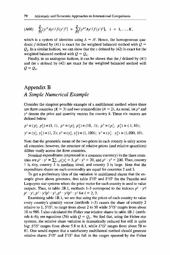
79 Axiomatic and Economic Approaches to International Comparisons
K K
j=1 k=l (A66) z[yiTAyjlf(yi)2] = z[ykTAyi/f(yi)2] , i = 1 , . . . , K ,
which is a system of identities using A = AT. Hence, the homogeneous qua- draticfdefined by (41) is exact for the weighted balanced method with Q = Q,. In a similar fashion, we can show that the c defined by (42) is exact for the weighted balanced method with Q = Q,.
Finally, in an analogous fashion, it can be shown that the f defined by (41) and the c defined by (42) are exact for the weighted balanced method with Q = Q,.
Appendix B A Simple Numerical Example
Consider the simplest possible example of a multilateral method where there are three countries (K = 3) and two commodities (N = 2). As usual, let pk and y' denote the price and quantity vectors for country k. These six vectors are defined below:
p' a (p;, p i ) I ( 1 , 1); p2 I ( p ? , p;) = (10, . l ) ; p3 = (p;, p i ) = (.1, 10);
yl = (yt, y;) = (1, 2); y2 = (y?, y;) = (1,100); y3 = (y?, y;) = (1,000,10).
Note that the geometric mean of the two prices in each country is unity across all countries; however, the structure of relative prices (and relative quantities) differs vastly across the three countries.
Nominal expenditures (expressed in a common currency) in the three coun- tries arepl * y1 = Xi=,p;yf, = 3, p2 * y2 = 20, andp3 y3 = 200. Thus, country 1 is tiny, country 2 is medium sized, and country 3 is large. Note that the expenditure shares on each commodity are equal for countries 2 and 3.
To get a preliminary idea of the variation in multilateral shares that the ex- ample given above generates, first table S2/S1 and S3/S for the Paasche and Laspeyres star systems where the price vector for each country is used to value outputs. Thus, in table lB.l, methods 1-3 correspond to the indexes p1 * y i / p1 * y', p2 * yi/p2 1 yl, p3 * yi/p3 * y1 for i = 2 , 3 .
Examining table 1B. 1, we see that using the prices of each country to value every country's quantity vector (methods 1-3) causes the share of country 2 relative to 1, WSl, to range from about 2 to 50 while S3/S ranges from about 10 to 980. I also calculated the Fisher star relative shares in table lB.l (meth- ods 4-6); see equations (56) with Q = QF. We find that, using the Fisher star systems, the relative share variation is dramatically reduced but still is quite big: S2/S ranges from about 5.8 to 8.1, while S3/S ranges from about 58 to 81. One would expect that a satisfactory multilateral method should generate relative shares S2/S1 and S3/S1 that fall in the ranges spanned by the Fisher

80 W. Erwin Diewert
stars-namely, 5.8-8.1 and 58-81, respectively. The Fisher blended shares de- fined by (57) are listed as method 7 in table lB.l.
In table 1B.2, I listed the exchange rate and average price and average quan- tity methods that were defined in sections 1.3-1.8 of the main text of this paper. Method 8 is the exchange rate method (see eqq. [l]). This method does rather well in this artificial model, probably because the geometric mean of prices in each country is identical. Hence, there are no grossly overvalued or under- valued country exchange rates. One would not expect this good performance to carry over to examples where some countries had grossly overvalued ex- change rates.
Turning now to the average price methods defined in section 1.4, we find that the arithmetic and geometric mean price methods defined by (15) and (1 6) generate equal average prices. Hence, both these methods are equivalent to method 1 in table 1B. 1, where the equal prices of country 1 were used to value quantities in each country.
Method 9 is the Walsh (1901,43 1)-Fisher (1922,307) arithmetic mean aver- age quantity method defined by (22) and (23), while method 10 the Walsh (1901, 398)-Gerardi (1982, 398) geometric mean average quantity method defined by (22) and (24). The arithmetic mean quantity vector turns out to be [334, 37.31, while the geometric mean quantity vector is [lo, 12.61. Thus, methods 9 and 10 generate quite different relative shares in table 1B.2.
The Geary (1958)-Khamis (1970) average prices method defined in section 1.6 is method 11. The vector of international prices (times 1,000) turns out to be [.4974, 4.47831, which is closest to the structure of relative prices in the large country, country 3. This method seems to lead to a tremendous overevalu- ation of the share of country 2; S 2 W for the GK method is 47.42157.35 = 33, which seems too large.
Van Yzeren’s (1956, 13) unweighted average price method defined in section 1.7 is the next method we consider. The international price vector [pT, p?] defined by (33) turns out to be [ l , 13, so, again, this method reduces to method 1. Van Yzeren’s (1956, 6-14) unweighted average quantity method defined in section 1.8 is method 12. The vector of average quantities defined by (43) for this method turns out to be [ yT, y:] = [.99342, 13. This method leads to a share for country 1 that is too large.
Table 1B.3 lists the superlative methods discussed in sections 1.9-1.12 with the bilateral Q equal to QF, the Fisher ideal quantity index.
The effects of weighting are evident in table 1B.3. The two superlative meth- ods that satisfy the country-partitioning test T10 (methods 15 and 16) have shares that are relatively close to the big country’s Fisher star shares (method 6), while the two superlative methods that do not satisfy T10 (methods 13 and 14) have shares that are very close to the arithmetic average of the Fisher star shares (method 7, a democratically weighted method).
The numerical example given above shows that the choice of a multilateral method is very important from an empirical point of view-more important

Table 1B.1 Paasche and Laspeyres Star and Fisher Star Systems
Method 1 Method 2 Method 3 Method 4 Method 5 Method 6 Method 7 (country 1 prices) (country 2 prices) (country 3 prices) (Fisher star 1) (Fisher star 2) (Fisher star 3) (blended Fisher)
SZIS' 33.67 1.96 49.76 8.12 8.12 5.79 7.25 S W 336.67 980.49 9.95 57.88 81.25 57.88 64.12
Table 1B.2 Exchange Rate and Average Price and Quantity Methods
Method 9 Method 10 Method 12 Method 8 (arithmetic mean (geometric mean Method 11 (Van Yzeren
(exchange rate) average quantities) average quantities) (Geary-Khamis) average quantities)
SZIS' 6.67 .74 1.49 47.42 1.32 S3IS' 66.67 60.86 11.86 51.35 13.16

82 W. Erwin Diewert
Table 1B.3 Superlative Methods Using the Fisher Bilateral Index
Method 13 Method 14 Method 15 Method 16 (Gini-EKS) (unweighted balanced) (own share) (weighted balanced)
S2ISl 7.2563 7.2563 6.024 6.001 S’/S1 64.8062 64.8062 59.970 59.697
than the choice of a bilateral index number formula in the time-series context because the variation in relative prices and quantities will usually be much greater in the multilateral context. Even when choosing between superlative multilateral methods, we see that there can be substantial differences between methods 13 and 14 (which pass the linear homogeneity test T8) and methods 15 and 16 (which pass the country-partitioning test T10).
If the quantity vector for country 1 is changed to y, = (’yi, yk) = (1, l) , then the expenditure shares on each commodity will equal 1/2 in each country. Hence, for this new data set, the data are consistent with economic agents maximizing the utility function f( yI, y,) = y:”y;” subject to country budget constraints. This functional form is a special case of (41) and (65) (with a,, = u2, = 0 and uI2 = 1/2), and, hence, the Fisher and Walsh bilateral quantity indexes defined by (2) and (64) will empirically pass the circularity test (52). (The direct and indirect Persons [ 1928, 21-22]-Tornqvist [ 19361 quantity in- dexes Q, and Q, defined in Diewert [1976, 120-211 will also pass the circular- ity test for this data set since Cobb-Douglas utility functions are exact for these functional forms as well.) For this modified data set, the entries in table lB.l for the Fisher star methods, methods 4-6, all reduce to S2/S1 = 10 and S3/S1 =
100. In this case, all the superlative methods listed in table 1B.3 also have S 2 / S = 10 and S3/S1 = 100. Thus, it is deviations from circularity of the bilat- eral index number formula that cause the superlative methods to yield different numerical results. As an aside, for this circular data set, it should be noted that the Geary-Khamis relative shares are S 2 / S = 90.13 and S3/S1 = 108.73. Thus, the share of country 2 still seems to be too large in this case. To further illus- trate that Geary-Khamis indexes can be quite different from Fisher ideal in- dexes, consider table 1B.4, where the Geary-Khamis bilateral index number formula (31) was used to form star system shares. The results using countries 1-3, respectively, as the base country are tabled in columns 1-3 and are com- pared with the common Fisher star shares in column 4.
I now return to the original noncircular data set and calculate the four super- lative indexes when I use the bilateral Walsh quantity index Q, defined by (64) in place of the bilateral Fisher quantity index Q, defined by (2).
In table 1B.5, I list the Walsh star shares S2/S1 and S3/S’ using countries 1-3 as the base (see eqq. [56], which define the star shares), which are methods 17-19. I also list the corresponding Fisher-Walsh blended shares defined by (57), where Q = Q , (method 20).

83 Axiomatic and Economic Approaches to International Comparisons
Table 1B.4 Geary-Khamis Star Shares versus Fisher Shares Using the Circular Data
Geary-Khamis 1 Geary-Khamis 2 Geary-Khamis 3 Fisher
S2IS' 2.92 S3IS' 20.76
2.92 3.50
17.34 10 20.76 100
Table 1B.5 Walsh Star Shares and Walsh Blended Shares
Method 17 Method 18 Method 19 Method 20 (Walsh star 1) (Walsh star 2) (Walsh star 3) (blended shares)
SVS' 9.167 9.167 5.238 7.603 SVS' 52.381 91.667 52.381 61.381
Table 1B.6 Superlative Methods Using the Walsh Bilateral Index
Method 21 Method 22 Method 23 Method 24 (Gini-Walsh) (unweighted balanced) (own share) (weighted balanced)
S2ISl 1.6067 7.6067 5.630 5.572 S'IS' 63.1227 63.1228 55.892 55.195
Comparing table 1B.5 with table lB.l, it can be seen that the Walsh star shares are less variable than the country price star shares (methods 1-3) but that the Walsh star shares (methods 17-19) are more variable than the Fisher star shares (methods 4-6). Thus, the Walsh star relative shares, S2/S', range from about 5.2 to 9.2 (while the corresponding Fisher variation was from 5.8 to 8.1), and the Walsh relative shares, S3/S', range from about 52 to 92 (while the corresponding Fisher variation was from 58 to 81). Since the Fisher indexes satisfy circularity better than the Walsh indexes, one would expect that the variation in the four Walsh superlative indexes will be greater than the variation in the four Fisher superlative indexes. This expectation is verified by the results of table 1B.6.
Comparing table 1B.6 with table 1B.3, we see some similarities: the demo- cratically weighted Gini-Walsh and Walsh unweighted balanced methods (methods 21 and 22) closely approximate each other, while the plutocratically weighted Walsh own share and Walsh weighted balanced methods (methods 23 and 24) also approximate each other reasonably closely. However, the spread between the methods that satisfy the linear homogeneity test T8 (methods 21 and 22) and the methods that satisfy the country-partitioning test T10 (methods 23 and 24) is much wider in table 1B.6 than it was in table 1B.3, where the more nearly circular Fisher bilateral indexes were used as the basic building blocks. In table 1B.6, note that the shares corresponding to the plutocratic meth-

84 W. Erwin Diewert ~~
Table 1B.7 International Prices Using Own Share Price Levels and GK Prices
Balk’s Method Hill’s Method Geary-Khamis
%IT, 8.895 9.028 9.003
ods 23 and 24 are closer to the shares of the big country star shares (method 19), whereas the shares corresponding to the equally weighted methods 21 and 22 are very close to the arithmetic average of the Walsh star shares (method 20).
The fact that, empirically, the Fisher bilateral indexes satisfy the circularity test more closely than the Walsh indexes reinforces the case for prefemng the Fisher index over its bilateral competitors. In addition to being superlative and satisfying more reasonable tests than its competitors, the Fisher ideal quantity index is the only superlative index that is consistent with (bilateral) revealed preference theory (see Diewert 1976,137). Thus, I prefer the Fisher superlative methods listed in table 1B.3 over the Walsh superlative methods listed in ta- ble 1B.6.
I conclude this appendix by calculating the international prices that were suggested at the end of section 1.13 for the noncircular data set.
Balk’s suggested vector of international prices r = (rI, r2) was defined by (86), and the generalized Hill prices were defined by (25), where the price levels (or purchasing power parities) Pk and the country shares Sk that appear in these equations were defined by the analyst’s “best” multilateral method. In table 1B.7, I used the Fisher own share Pk and Sk (see method 15 in table 1B.3) in equations (86) and (25) to calculate the Balk and Hill international prices. Both these international price relatives rJr1 are close to the Geary-Khamis international price relative, r2hI = 9.004. Recall that the structure of relative prices in the three countries is pilp; = 1, pyp: = .01, and p:/p: = 100 for countries 1-3, respectively. Thus, the international price ratios in table 1B.7 all tend to lean toward the structure of relative prices in the big country, country 3. Note that, if I used the Balk or Hill international prices to value the quantity vectors in each country, the resulting country shares of world consumption at these constant prices would be very close to the Geary-Khamis shares (see method 11 in table 1B.2), and these shares are very different from the shares generated by the suggested best methods listed in table 1B.3.
The numerical example suggests that additive multilateral methods should not be used if the structure of relative prices is very different across countries. In this case, no single international price vector can adequately represent the prices faced by producers or consumers in each country. In order to model adequately the very large substitution effects that are likely to be present in this situation, an economic approach based on the use of superlative indexes should be used.

85 Axiomatic and Economic Approaches to International Comparisons
References
Afriat, S. N. 1967. The construction of utility functions from expenditure data. Interna-
Armstrong, K. G. 1995. Multilateral approaches to the theory of international compari-
Balk, B. M. 1989. On Van Ijzeren’s approach to international comparisons and its prop-
. 1995a. Axiomatic price index theory: A survey. International Statistical Re-
. 199%. On the use of unit value indices as consumer price subindices. Voor-
. 1996. A comparison of ten methods for multilateral international price and
Debreu, G., and I. N. Herstein. 1953. Nonnegative square matrices. Econometrica
Diewert, W. E. 1971. An application of the Shephard duality theorem: A generalized
. 1974. Functional forms for revenue and factor requirements functions. Interna-
. 1976. Exact and superlative index numbers. Journal of Econometrics 4:
. 198 1. The economic theory of index numbers: A survey. In Essays in the theory and measurement of consumer behavior in honour of Sir Richard Stone, ed. A. Dea- ton. London: Cambridge University Press.
. 1986. Microeconomic approaches to the theory of international comparisons. Technical Working Paper no. 53. Cambridge, Mass.: National Bureau of Economic Research.
. 1988. Test approaches to international comparisons. In Measurement in eco- nomics, ed. W. Eichhorn. Heidelberg: Physica.
. 1992. Fisher ideal output, input and productivity indexes revisited. Journal of Productivity Analysis 3:211-48.
. 1993a. Duality approaches to microeconomic theory. In Essays in index num- ber theory, vol. 1, ed. W. E. Diewert and A. 0. Nakamura. Amsterdam: North- Holland.
. 1993b. The early history of price index research. In Essays in index number theory, vol. 1, ed. W. E. Diewert and A. 0. Nakamura. Amsterdam: North-Holland.
. 1993c. Symmetric means and choice under uncertainty. In Essays in index number theory, vol. 1, ed. W. E. Diewert and A. 0. Nakamura. Amsterdam: North- Holland.
. 1995. Axiomatic and economic approaches to elementary price indexes. Dis- cussion Paper no. 95-01. University of British Columbia, Department of Economics.
. 1996. Price and volume measures in the system of national accounts. In The new system of national accounts, ed. J. W. Kendrick. Boston: Kluwer Academic.
Dikhanov, Y. 1994. Sensitivity of PPP-based income estimates to choice of aggregation procedures. Paper presented at the conference of the International Association for Research in Income and Wealth, St. Andrews, New Brunswick, August.
Drechsler, L. 1973. Weighting of index numbers in multilateral international compari- sons. Review of Income and Wealth, ser. 19 (March): 17-47.
Eichhorn, W. 1976. Fisher’s tests revisited. Econometrica 44:247-56.
Eichhorn, W., and J. Voeller. 1976. Theory of the price index. Berlin: Springer.
tional Economic Review 8:67-77.
sons. Ph.D. diss., University of British Columbia.
erties. Statistische Hefte 30:295-315.
view 63:69-93.
burg: Statistics Netherlands, Division of Research and Development, 14 March.
volume comparisons. Journal of Oficial Statistics 12: 199-222.
21 1597-607.
Leontief production function. Journal of Political Economy 79:48 1-507.
tional Economic Review 15: 119-30.
115-45.
. 1978. Functional equations in economics. London: Addison-Wesley.

86 W. Erwin Diewert
Elteto, O., and P. Koves. 1964. On a problem of index number computation relating to
Fisher, I. 191 1. The purchasing power of money. London: Macmillan.
Frisch, R. 1930. Necessary and sufficient conditions regarding the form of an index number which shall meet certain of Fisher’s tests. American Statistical Association Journal 25:397-406.
Frobenius, G. 1908. Uber Matrizen aus positiven Elementen. Sitzungsberichte der kiinig- lichpreussischen Akademie der Wissenschafen, pt. 1:471-76. Berlin: Royal Prussian Academy of Sciences.
. 1909. Uber Matrizen aus positiven Elementen 11. Sitzungsberichte der kiinig- lichpreussischen Akademie der Wissenschafen, pt. 1:s 14-1 8. Berlin: Royal Prussian Academy of Sciences.
Gale, D., and H. Nikaido. 1965. The Jacobian matrix and the global univalence of map- pings. Muthematische Annalen 159:81-93.
Geary, R. G. 1958. A note on comparisons of exchange rates and purchasing power between countries. Journal of the Royal Statistical Society A 121 :97-99.
Gerardi, D. 1974. Sul problema della comparazione dei poteri d’acquisto delle valute. Serie papers. Instituto di Statistica dell’universita di Padova, August.
. 1982. Selected problems of inter-country comparisons on the basis of the expe- rience of the EEC. Review of Income and Wealth, ser. 28:381-405.
Gini, C. 1924. Quelques considCrations au sujet de la construction des nombres indices des prix et des questions analogues. Metron 4, no. 1:3-162.
international comparisons. Statisztikai Szemle 42507-1 8.
. 1922. The making of index numbers. Boston: Houghton Mifflin.
. 1931. On the circular test of index numbers. Metron 9, no. 9:3-24.
. 1946. Value and capital. 2d ed. Oxford: Clarendon. Hicks, J. R. 1940. The valuation of the social income. Economica 7:105-40.
Hill, R. J. 1995. Purchasing power parity methods of making international compari-
Hill, T. P. 1982. Multilateral measurements ofpurchasingpower and real GDl? Luxem-
. 1984. Introduction: The Special Conference on Purchasing Power Parities. Re-
IklC, D. M. 1972. A new approach to the index number problem. Quarterly Journal of
Jevons, W. S. 1884. Investigations in currency and finance. London: Macmillan. Karlin, S. 1959. Mathematical methods and theory in games, programming and eco-
nomics. Vol. 1. Reading, Mass.: Addison-Wesley. Khamis, S. H. 1970. Properties and conditions for the existence of a new type of index
number. Sankhya B32:8 1-98. . 1972. A new system of index numbers for national and international purposes.
Journal of the Royal Statistical Society A135:96-121. Kravis, I. B. 1984. Comparative studies of national incomes and prices. Journal of Eco-
nomic Literature 22: 1-39. Kravis, I. B., Z. Kenessey, A. Heston, and R. Summers. 1975. A system of international
comparisons of gross product andpurchasingpowel: Baltimore: Johns Hopkins Uni- versity Press.
Kravis, I. B., R. Summers, and A. Heston. 1982. Comments on “Selected problems of intercountry comparisons on the basis of the experience of the EEC.” Review of In- come and Wealth, ser. 28:407-10.
Kurabayashi, Y., and I. Sakuma. 1990. Studies in international comparisons of real products and prices. Hitotsubashi University, Institute of Economic Research, Eco- nomic Research Series no. 28. Tokyo: Kinokuniya.
Leontief, W. 1936. Composite commodities and the problem of index numbers. Econo- metrica 4139-59.
sons. Ph.D. diss., University of British Columbia.
bourg: Eurostat.
view of Income and Wealth, ser. 30:125-33.
Economics 86:188-211.

87 Axiomatic and Economic Approaches to International Comparisons
Marris, R. 1984. Comparing the incomes of nations: A critique of the international
Martini, M. 1992. A general function of axiomatic index numbers. Journal of the Italian
Perron, 0. 1907. Grundlagen fur eine Theorie des Jacobischen Kettenbruchalgorith-
Persons, W. M. 1928. The construction of index numbers. Cambridge, Mass.: Riverside. Pierson, N. G. 1896. Further considerations on index-numbers. Economic Journal 6:
Reinsdorf, M. B., and A. H. Dorfman. 1995. The Sato-Vartia index and the monoton-
Rudin, W. 1953. Principles of mathematical analysis. New York: McGraw-Hill. Sato, K. 1976. The ideal log-change index number. Review of Economics and Statis-
Shephard, R. W. 1953. Cost and production functions. Princeton, N.J.: Princeton Uni-
Szulc, B. 1964. Indices for multiregional comparisons. Przeglad Statystyczny 3:239-54. Tomqvist, L. 1936. The Bank of Finland’s consumption price index. Bank of Finland
Van Yzeren, J. 1956. Three methods of comparing the purchasing power of currencies.
Van Ijzeren, J. 1983. Index numbers for binary and multilateral comparison. Statistical
Van Ijzeren, J. 1987. Bias in international index numbers: A mathematical elucidation.
Vartia, Y. 0. 1974. Relative changes and economic indices. Licenciate thesis, Depart-
. 1976. Ideal log-change index numbers. Scandinavian Journal of Statistics 3:
Vogt, A. 1980. Der Zeit und der Faktorumkehrtests als “Finders of Tests.” Statistiche
Walsh, C. M. 1901. The measurement of general exchange value. New York Mac-
. 1921. Discussion of the best form of index number. Journal of the American
comparison project. Journal of Economic Literature 22, no. 1 :40-57.
Statistical Society 3:359-76.
mus. Mathematiscke Annalen 64: 1-76.
127-3 1.
icity axiom. Washington, D.C.: U.S. Bureau of Labor Statistics.
tics 58:223-28.
versity Press.
Monthly Bulletin 10: 1-8.
Statistical Studies no. 7. The Hague: Netherlands Central Bureau of Statistics.
Studies no. 34. The Hague: Netherlands Central Bureau of Statistics.
Eindhoven: Dissertatiedrukkerij Wibro.
ment of Statistics, University of Helsinki.
121-26.
Hefte 21:66-71.
millan.
Statistical Association 17537-44. Westergaard, H. 1890. Die Grundziige der Theorie der Stutistik. Jena: Fischer. Wold, H. 1944. A synthesis of pure demand analysis, part 111. Skandinavisk Aktuarietid-
skrift 27:69-120.
Comment Irwin L. Collier Jr.
Erwin Diewert has produced another magnificent paper. One could say that this work is genuinely Fisheresque, both in its comprehensiveness and in its dogged pursuit of relevant detail. All that is missing is a sprinkling of the homely touches that distinguish Irving Fisher’s work on index numbers and economics in general, for example, a comparison of the precision of quantify-
Irwin L. Collier Jr. is professor of economics at the Freie Universitat Berlin.

88 W. Erwin Diewert
ing the purchasing power of money with the precision of measuring the height of the Washington Monument. Instead, Diewert packs his results modestly in the streamlined style of present-day economic theory He takes us farther faster so that we may have more time to do what we have to do once we get there, assuming that we knew where we wanted to go in the first place. It is the discussant’s job to help the hurried traveler distinguish a few landmarks in the blur of Diewert’s forward motion.’
Ten classes of multilateral index number methods are rigorously examined, and four of the methods actually succeed in winning the Diewert seal of ap- proval on a combination of axiomatic merits and economic flexibility. This is the immediate contribution of this paper to the debate on multilateral index number methods. Since there will be undoubtedly future contenders for the title of best multilateral method, the lasting value of Diewert’s paper will be found in the testing procedures implemented as well as their careful documen- tation by Diewert in his appendix A. These proofs will help future index for- mula inventors and users judge for themselves.
The axiomatic method is similar to the Ten Commandments approach to virtue. Good people honor their fathers and mothers and do not covet their neighbors’ goods, and good index numbers do not change their values simply because we change our units of measurement from pounds to ounces (T4) or our price measurements from dollars to cents (T7). Diewert’s tablets in fact list eleven tests, but most of his followers will probably regard them as ten com- mandments plus a normalization condition (thou shalt have output shares that add up to unity, Tl).
There are several reasons why composing lists of index number axioms is both a satisfying and a worthwhile task in economic measurement.
One important reason is that we are practical only once we become specific in these matters. An axiom that “the index number should not be misleading” is as worthless as a commandment that “thou shalt not be evil.” “Nobody is special” (T6) and “no commodity is special” (T5) are the sort of axioms that should indeed receive immediate and unanimous agreement and ones where a violation is immediately demonstrated whenever the simple act of swapping i , j country superscripts or commodity subscripts leads to a change in a country’s relative performance. Of course, a potential danger in getting specific is that our list of tests can begin to grow and approach the length of a checklist for a space shuttle liftoff.
This leads to another reason why this approach is both satisfying and worth- while. The act of whittling down a list of axioms involves distinguishing those axioms that are in some sense fundamental from those that can be derived from subsets of the fundamental axioms. Here, the point is not checking whether a
1. Actually, Diewert himself provides his passengers an excellent aid for orientation with his simple numerical example that works through an artificial three-country, two-good case. The impa- tient reader who has jumped this far forward should mark those pages to consult during a detailed reading of Diewert’s paper.

89 Axiomatic and Economic Approaches to International Comparisons
particular formula complies with the tests but instead analyzing the interaction of the tests among themselves. This aspect of the axiomatic approach to inter- national comparisons is not touched on in this particular paper.2
Index number formulas and tests are like people and commandments; one need not look very far to find seemingly simple rules in conflict with each other. Since it is natural for economists to think in terms of choice between competing goods, this is hardly the stuff of tragedy. In section 1.13, Diewert proves that he is a wise judge, much as appendix A reveals him to be a strict judge.
The choice of an index number formula for a multilateral comparison is analogous to the problems of designing a voting procedure for multicandidate/ issue elections, a system to rank competing athletic teams in a league, or a method to aggregate the opinions of independent expert^.^ There is an essential difference in that most of these other problems seek nothing more than an ordinal ranking (A gets the gold medal, B the silver, and C the bronze), whereas the business of multilateral comparisons of real income and product loses most, if not all, of its charm should it fail to deliver an answer to the question just how much closer B is to A than C. It is hardly coincidental that the axiomatic method plays a prominent role in all these areas.
Useful in thinking about such problems is the presumed existence of some underlying latent variable of real consumption or production (the concern of this volume) or of performance/ability/political strength (such as when a uni- versity department votes to rank job candidates). Here is where the economic approach to international comparisons enters the picture. Working backward from the actual latent index of real consumption, one easily calculates a con- sistent matrix of bilateral comparisons. We adopt the convention of assigning the column country in each binary comparison the role of base country (the de- nominator of the ratio). To illustrate, suppose that the true shares of world out- put are those given in the lean-truth vector in table lC. l . One can immediately verify that each column of the fat-truth matrix is the lean-truth vector divided by one of the country values. Some of the values are completely uninformative; the diagonal of ones will be found for all fat-truth matrices. Furthermore, there is a redundancy between elements located above and below the diagonal. Obvi- ously, the lean-truth vector can be calculated from any single row or column of the fat-truth matrix.
One very good reason for thinking about the truth in terms of a matrix of binary comparisons is that the analyst is often given something related to the true matrix of binary comparisons. Many (although not all!) of the methods of multilateral comparison attempt to find the lean-truth vector hiding inside a fat matrix of actual binary comparisons. Returning to the related problems just
2. For an example of this sort of work, see Eichhorn and Voeller (1990). 3. For an entry point into this literature, one can consult David (1988) as well as the papers in
Fligner and Verducci (1993)-in particular the paper by Stem (1993)-that give a statistical twist. Young (1995) offers a very readable survey of voting mechanisms.

90 W. Erwin Diewert
Country 1 .10 Country 2 .30 Country 3 .60
Table lC.l A True Multilateral Vector Generates a Single True Matrix of Bilateral Comparisons
Country 1 1 .oo .33 .17 Country 2 3.00 1.00 .50 Country 3 6.00 2.00 1 .oo
Lean-Truth Vector
Fat-Truth Matrixa ~~
Country 1 Country 2 Country 3
Table 1C.2 Empirical Bilateral Comparisons Generate Multiple Multilateral Vectors
Fisher Quantity Index
Country Country Country 1 2 3
Country 1 1.000 .121 .017 Country 2 8.125 1.000 ,100 Country 3 57.879 10.000 1 .ooo
Three Versions of the Truth
First Second Third “Truth” “Truth” “Truth
Country 1 1.000 1.000 1.000 Country 2 8.125 8.125 5.788 Country 3 57.879 81.248 57.879
mentioned, in the public choice literature, such matrix entries could be the actual outcomes of head-to-head elections, or, in the problem of ranking indi- vidual chess players, these could be the outcomes of games between pairs of players at a tournament. As we see from the matrix of Fisher quantity indexes taken from Diewert’s example (see table 1C.2), each of the Fisher columns is consistent only with a different lean-truth vector. This is precisely the sort of discrepancy that led Irving Fisher to reach for his statistical blender (Diewert’s method 7).
There are plenty of bilateral index formulas that one might have chosen, and one is not necessarily limited to any one matrix of binary comparisons. Thus, it was entirely appropriate for Diewert to think about the appropriate choice of binary indexes for many of the multilateral methods. One should also note that one might choose to work with less information than a complete bilateral comparison matrix or that one might work with the entire set of underlying price and quantity data. An interesting structural characteristic of the differing multilateral methods is the degree of disaggregation in the underlying data that is required for their calculation. The four methods favored in the end by Die- wert are all generated directly from a matrix of binary comparisons. In con- trast, the well-known Geary-Khamis system, a method that did not make it into Diewert’s final four, requires a finer disaggregation of the expenditure and quantity data.
With an eye to the aggregation requirements in a computational sense, I now look at the ten classes of multilateral methods examined by Diewert. This will

91 Axiomatic and Economic Approaches to International Comparisons
involve traveling a slightly different route, one that takes us from the minimum to the maximum disaggregation of the underlying price and quantity data. The minimum disaggregation method is also the method that Diewert chose to eval- uate first.
The data requirements for the exchange rate method are so minimal that one need not actually compare anything to set up shop-a list of nominal expendi- tures, along with a list of exchange rates, is enough to become a comparisons consultant. Sure, one must divide nominal expenditures in one country by nominal expenditures in another to obtain a kind of binary comparison. No pain, no gain. But the reason that Laspeyres and Paasche started us all wor- rying about index numbers is the fact that ratios of nominal values confound price with quantity changes. Diewert is able to keep a straight face testing “probably the most commonly used method for making multilateral compari- sons.” The man is a professional. It is appropriate to include under this method all attempts to unlock nominal expenditures with a single price, such as the Economist’s tongue-in-cheek (maybe) Big-Mac-Index.
The next set of indexes constitutes the so-called star systems, which are simply single columns (normalized to sum to unity) plucked from the Las- peyres, Fisher, Geary-Khamis (bilaterals), or Walsh quantity index matrices. One column from any of these matrices represents a considerable information advance compared to the exchange rate method since a revaluation of market baskets actually takes place. On the other hand, it is quite obvious that other columns need never be calculated once the role of the star country has been cast. In table lC.2, the three columns on the right correspond to Fisher star 1-3 in Diewert’s numerical example. Any one column is distinguished from the other columns by the asymmetrical treatment given the country chosen as the base country in the binary comparisons. In the first column, all countries are compared to country 1, in the second column to country 2, and in the third column to country 3. One significant reason for the Eastern European origins of the EKS method in multilateral international comparisons was a political desire to have a reason for knocking the Soviet Union out of its key role as base country in all CMEA (Council for Mutual Economic Assistance) comparisons, making things a little more mutual, at least in a statistical sense.
The three columns on the right of table 1C.2 represent three different points on the unit simplex, the geometric representation of the normalization of world output equal to 100 percent. In figure lC.l , three such points are plotted (that have been drawn to correspond to different underlying data in the interests of visual clarity). Since there is no objective reason to favor one base country over another, one can see why Irving Fisher would have thought of (implicitly) finding that point on the unit simplex that was closest to the three points of the Fisher star system. An unweighted arithmetic averaging of the coordinates of the original three points is what Diewert has listed as method 7 in his appendix B. The first thing to note is that the blended Fisher index requires knowledge

92 W. Erwin Diewert
s3
Fig. lC.l different base countries
Points on the unit simplex are normalized Fisher quantity indexes for
of the entire Fisher quantity index matrix, making it really the first of the multi- lateral methods we meet that exploits all the information from a bilateral com- parisons matrix. Hence, while it is logical in one sense to place the blended Fisher in a table next to the stars that generated it, it turns out (as Diewert indeed notes) to be numerically a next-door neighbor to the unweighted super- lative indexes (Gini-EKS and unweighted balanced) in his table 1B.3. This proximity, along with the fact that the blended Fisher index is the outcome of an explicit minimization problem (i.e., minimizing the sum of squared dis- tances from the three stars on the simplex), would have made it an outstanding candidate for an axiomatic and economic testing by Diewert. Instead, it is left as an interesting exercise for the reader.
However, before moving on to consider other formulas that blend an entire matrix of binary comparisons into a single multilateral index, there are two relatively primitive methods discussed by Diewert that start by blending the price or quantity data before any comparisons are attempted. This is a rela- tively unimaginative way to eliminate the inconsistency between individual binary comparisons calculated with only one or two of the K different columns from the N X K matrices of prices and quantities. In table 1C.3, one can di- rectly compare the i , jth elements of the bilateral quantity comparisons from the multilateral symmetric means methods with their respective Laspeyres bi- lateral comparisons. In the first row, the average price method is compared to the corresponding Laspeyres quantity index, and, in the second row, the aver- age quantity method index is compared with the Laspeyres quantity index ob- tained by deflating nominal expenditures with a Paasche price index.
In the first row of table 1C.3, one can see that the prices used in the Las- peyres matrix (which differ for each columnj) have been replaced by an aver-

93 Axiomatic and Economic Approaches to International Comparisons
Table 1C.3 Average Price and Average Quantity Methods Compared to Laspeyres Bilateral Indexes and the Geary-Khamis Multilateral Index
Bilateral Laspeyres Quantity Index
N c PLY:,
c P’,Yi
P>
“=I V
“=I
N c YLP’, ?iL
p J . Y J c Y’P: ” ~ I
Symmetric Means Methods
n
Using average c rn(P,JY:,
c rn(P,)YL
? ? = I prices n
n = l
N
Using average c rn(YJP:, P‘ . Y‘ n = l quantities
P’ ’ Y’ 2 m(yn)p: . ,=I
Geary-Khamis Method
age of K country prices. Similarly, the quantities used in the (inverse of the) Paasche price index in the second row have been replaced by an average of K country q~antit ies.~ Diewert rightly remarks that the Geary-Khamis method is a “more complex average price method,” and his discussion of the Geary- Khamis method immediately follows his own discussion of the symmetric means methods. In my opinion, the far greater complexity of the Geary- Khamis international prices puts the GK method into an entirely different class. The so-called international prices used to value the country quantities (in the first row of table 1C.3) are functions, not just of p , (a single column of the p matrix), but of the entire p and y matrices together.
Returning to our lean-truth vector from a fat-truth matrix extraction prob- lem, the first two methods based on a complete matrix of binary comparisons that Diewert analyzes are Van Yzeren’s unweighted average price (UAP) and unweighted average basket (UAB) methods. Diewert notes a certain similarity between the UAP and the Geary-Khamis definition of average bloc prices. However, from the standpoint of price and quantity disaggregation, the differ- ence is really what counts. The fact that the UAP method does not employ quantity weights in averaging the (purchasing power parity-deflated) individ- ual country prices is the reason that one is able to work at the level of the matrix of binary comparisons. This can be seen immediately in Diewert’s use- ful reformulation of the UAP (eqq. [39], [40]) and UAB (eqq. [49], [50]) sys- tems. Although not explicitly identified as such, the D matrix in Diewert’s re- formulation is nothing other than the matrix of Laspeyres quantity indexes:
D {(p’ . y’ ) - ’ (p’ . y’)}.
4. It will be recalled that the exchange rate method required the N-vector of nominal expenditures and the N-vector of exchange rates. The average price method requires the original N X K matrix of quantities, y, and an N-vector of average prices. The average quantity method requires the original N X K matrix of prices, p , an N-vector of average quantities, and the N-vector of nominal expendi- tures.

94 W. Erwin Diewert
An appropriately normalized eigenvector from D is shown by Diewert to be the UAP multilateral quantity index. He also proves that an eigenvector from the matrix transpose of D can be used to calculate the multilateral quantity index for the UAB method. Thus, two of the Van Yzeren methods appear to offer an alternative to the statistical approach of a Fisher blending of the col- umns of a matrix of binary comparisons. However, it is hardly obvious to this Perron-Frobenius-challenged reader which economic or even statistical truth the positive eigenvector pulled from a Laspeyres matrix of bilateral compari- sons (or its transpose) is actually trying to tell us. Diewert shows that it is not an exact truth for the flexible functional forms defined by his equations (41) and (42).
One of the puzzles in Diewert’s appendix B are the identical values in table 1B.3 calculated using the Gini-EKS formula (eq. [63]) and Van Yzeren’s un- weighted balanced method (UBM) (eq. [74]). Since Gini’s priority is indisput- able, one should abbreviate this to GEKS. Anyone who goes to the trouble of checking these calculations will find that the agreement continues for many more digits than shown in the table. This is not simply an artifact of the particu- lar numbers chosen for the example. Diewert attributes this “similarity” to an approximation of arithmetic means by geometric means. There is in fact a better argument for treating GEKS and UBM as a single method, at least for economic data from this world. One should not be too surprised that they have identical axiomatic and “economic” properties-they are “approxi- mately” identical twins.
The source of the near identity of the methods can be seen once we write the minimization problems behind the respective formulas in such a way as to reveal the particular loss functions that turn out not to be so very different at all. First, restate the minimization problems as found in Diewert’s paper:
(UBM[711) mins, , S K ZZQW, p J , yk, y J ) S k l S J , K K
’ j=1 k=l
The UBM minimization problem can be easily rewritten to highlight a distinct family resemblance to the GEKS:
(71‘)
Instead of the conventional quadratic loss function used in (61), Van Yzeren’s UBM uses an asymmetric loss function, the exponential. However, the asym- metry is apparent only as long as the underlying bilateral index numbers satisfy the country reversal test, as do the Fisher bilateral indexes. If we rewrite (7 1 ’) by grouping the (k , j ) terms with their ( j , k ) partner terms and exploit the country reversal test, we obtain
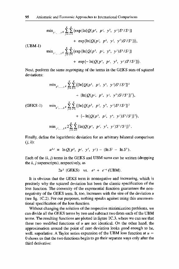
95 Axiomatic and Economic Approaches to International Comparisons
Finally, define the logarithmic deviation for an arbitrary bilateral comparison ( j , k):
uk,l = lnQ(pk, p ’ , y k , y ’ ) - (Ins’ - Insk ) .
Each of the ( k , j ) terms in the GEKS and UBM sums can be written (dropping the k, j superscripts), respectively, as
2u2 (GEKS) vs. e” + e-‘ (UBM).
It is obvious that the GEKS term is nonnegative and increasing, which is precisely why the squared deviation has been the classic specification of the loss function. The convexity of the exponential function guarantees the non- negativity of the GEKS term. It, too, increases with the size of the deviation u (see fig. 1C.2). For our purposes, nothing speaks against using this unconven- tional specification of the loss function.
Without changing the solution of the respective minimization problems, we can divide all the GEKS terms by two and subtract two from each of the UBM terms. The resulting functions are plotted in figure 1C.3, where we can see that these two modified functions of u are not identical. On the other hand, the approximation around the point of zero deviation looks good enough to be, well, superlative. A Taylor series expansion of the UBM loss function at u =
0 shows us that the two functions begin to go their separate ways only after the third derivative:
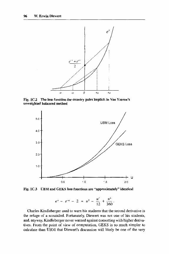
96 W. Erwin Diewert
Fig. 1C.2 The loss function for country pairs implicit in Van Yzeren’s unweighted balanced method
4.0
0.5 1 .o 1.5 2 0
Fig. 1C.3 UBM and GEKS loss functions are “approximately” identical
u4 u6
12 360 eu + e-u - 2 3 u2 + - i- -.
Charles Kindleberger used to warn his students that the second derivative is the refuge of a scoundrel. Fortunately, Diewert was not one of his students, and, anyway, Kindleberger never warned against consorting with higher deriva- tives. From the point of view of computation, GEKS is so much simpler to calculate than UBM that Diewert’s discussion will likely be one of the very

97 Axiomatic and Economic Approaches to International Comparisons
last sightings of this Rube Goldberg model index number, a nice example of overengineering (of course nondeliberate) in empirical economics.
Having just reunited one pair of twins found in Diewert’s paper, one will perhaps be less surprised that there happens to be a pair of half siblings living separate lives in this paper as well. It turns out that Diewert’s own share method (DOS) and the weighted balanced method (WBM) of Van Yzeren are linked by a common loss function, although one must challenge the legitimacy of the latter’s claim in mathematical court. The two methods can be motivated by considering the problem of minimizing the weighted sum of the expression that we have just encountered in the UBM method:
Suppose that one believes that it would be appropriate to use the yet-to-be- estimated shares as the weights in the minimization problem, wi = Si.5 Diewert tells us that Van Yzeren makes this substitution, but only after deriving the first-order conditions that are used to define his WBM. The reason for WBM’s illegitimacy (in a mathematical sense) is that one may not derive the first-order conditions for (7 1) with respect to the S parameters as though the weights were constant and then ex post substitute the S’s into the first-order conditions for the weights to calculate the index. The easy way to demonstrate that (71) was not minimized this way is to take the figures from Diewert’s example for WBM in his table 1B.3 and plug them directly into (71). The numerical value is 1.2356. The S parameters obtained from the DOS method in Diewert’s table 1B.3 give a lower value, 0.9999. As seen in Diewert’s tables 1B.3 and 1B.6, the WBM numbers are nonetheless quite close to those from the DOS method.
Now suppose that we decide instead to try to be right for the right reasons and substitute the weights into (71) from the start. This simplifies the minimi- zation problem enormously:
where the last summation is the column sum of the underlying binary index matrix, and things are beginning to look suspiciously like the DOS method.
To enforce the normalization, rewrite the problem as the minimization of the Langrangian expression:
After deriving the ith first-order condition, solve for the quantity index:
5. The appropriateness of these weights is by no means obvious.
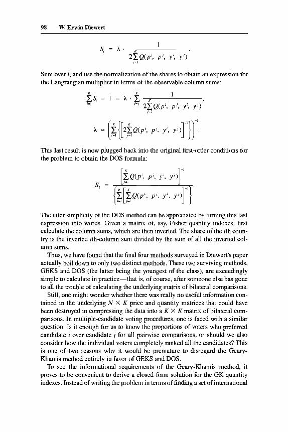
98 W. Erwin Diewert
Sum over i, and use the normalization of the shares to obtain an expression for the Langrangian multiplier in terms of the observable column sums:
This last result is now plugged back into the original first-order conditions for the problem to obtain the DOS formula:
si =
The utter simplicity of the DOS method can be appreciated by turning this last expression into words. Given a matrix of, say, Fisher quantity indexes, first calculate the column sums, which are then inverted. The share of the ith coun- try is the inverted ith-column sum divided by the sum of all the inverted col- umn sums.
Thus, we have found that the final four methods surveyed in Diewert's paper actually boil down to only two distinct methods. These two surviving methods, GEKS and DOS (the latter being the youngest of the class), are exceedingly simple to calculate in practice-that is, of course, after someone else has gone to all the trouble of calculating the underlying matrix of bilateral comparisons.
Still, one might wonder whether there was really no useful information con- tained in the underlying N X K price and quantity matrices that could have been destroyed in compressing the data into a K X K matrix of bilateral com- parisons. In multiple-candidate voting procedures, one is faced with a similar question: Is it enough for us to know the proportions of voters who preferred candidate i over candidate j for all painvise comparisons, or should we also consider how the individual voters completely ranked all the candidates? This is one of two reasons why it would be premature to disregard the Geary- Khamis method entirely in favor of GEKS and DOS.
To see the informational requirements of the Geary-Khamis method, it proves to be convenient to derive a closed-form solution for the GK quantity indexes. Instead of writing the problem in terms of finding a set of international

99 Axiomatic and Economic Approaches to International Comparisons
prices and purchasing power parities (PPPs), modify the method so that inter- national expenditures and country quantity indexes become the variables that are determined by the system of Geary-Khamis equations.
Start with the familiar N Geary-Khamis international price equations:
The trained eye immediately spots the weighted averages of PPP-adjusted country prices, where the weight of the kth term is equal to the kth country's share of the aggregate quantity of good n. Summations of goods across coun- tries are designated by dropping the country superscript:
K
Y" = CYl. k=l
However, instead of proceeding to define K PPP equations for the unknown Pk terms in equation (25), as is usually done, we may easily transform these international price equations into international expenditure equations. Multi- ply each side of the N equations in (25) with the corresponding total quantities of the countries in the comparison, thereby eliminating that term from the de- nominator of the right-hand side of (25). Next, divide and multiply each of the k terms of the sum by total expenditure in the kth country, and rearrange to obtain a new weighted average:
where the quantity index for country k is defined by deflating nominal expendi- tures with the PPP index (cf. Diewert's eq. [20]). International expenditures on the nth good in the Geary-Khamis system are defined to be the weighted aver- age of the budget shares (the weights have become the weighted!) of the N goods in the K countries, w:, where country quantity indexes, Sk, have been used as weights. It is important to note that we treat the product T,Y, as an unknown variable in this system of equations. To calculate international prices later, one only need divide the derived international expenditures by the appro- priate y,.
The second modification of the traditional Geary-Khamis system is to re- arrange equation (26) to obtain K equations for the country quantity indexes, Sk, expressed as weighted averages of each country's respective shares of world quantities, vi:

100 W. Erwin Diewert
Writing (25' ) and (26') in matrix notation, one can see the raw material out of which Geary-Khamis indexes are manufactured: an N X K matrix of country budget shares (columns sum to unity) and a K X N matrix of the structure of world consumption by countries (columns likewise sum to unity):
Defining the matrices W = [ w l ] , V = [vk], z = [ ~ r ~ y , ] , s = [ P I , the alternate Geary-Khamis multilateral system can be compactly written as
(GK-1) z = ws, s = V T Z .
Substituting the country real consumption (output) equations (s) into the inter- national expenditure equations (z) , we obtain
z = w v T z , which can be written
(GK-2) 0, = [ I , - wv'lz.
One might stop at the first of the last two equations and think of z as an eigenvector of the matrix WV', or one might look at the second equation and wish that there were something other than a zero vector on the left-hand side so that the matrix expression in brackets could be inverted and solved for z .
However, the matrix expression in brackets is not invertible since the matrix difference I , - WVT can easily be seen to be singular, which is definitely for the good since, otherwise, the international expenditure vector z would really have to stand for the zero vector.
To demonstrate the singularity of I , - WV', consider an element i , j of WVT,
w, = [ w : ,..., w f ; ] , theithrowof W ,
v: = [v:,. . . , v:]', thejth column of V T ,
K
[wv'],,, = w,v; = Cw";. k=l

101 Axiomatic and Economic Approaches to International Comparisons
Summing over i, we obtain the sum of the elements of thejth column:
The sum of each column of the identity matrix is likewise equal to unity. Thus, the sum of each of the columns of IN - WVT is zero (i,e., 1 - 1 = 0), and therefore the sum of any K - 1 rows is equal to the negative of the remaining row. Therefore, the matrix IN - WVT is singular.
Fortunately, the singularity of a matrix is a rather special circumstance, much as the zero point on the number line is pretty special. This means that fairly minor changes to the matrix WVT can destroy its singularity, and that would allow us to invert the new matrix in the process of solving the matrix equation for z. The trick here is to add a normalization condition on the s vector that will also help us eliminate the problem of having a zero vector on the left- hand side of (GK-2).
A convenient normalization is to set the value of world quantities equal to some constant. Like Diewert, I normalize the value of world output to be equal to unity:
I l d
a constraint that can be written in matrix form,
where c = [l 0 . . . OITis an N X 1 vector, and
R = 1 !. ::: ;] is an N x N matrix.
... ...
Now we add the constraint matrix equation to the original matrix equation,
(GK-3) c = [ZN - WVT + R]z .
By adding a one to each element of the first row of the original singular matrix, the sum of any column of IN - WVT + R is now unity, thus eliminating the original dependency among the rows. This will be enough to get nonsingularity into the bracketed expression in (GK-3), and we can solve (GK-3) for the inter- national expenditure vector z:
(GK-4) z = [ I N - WVT + R]-'c.

102 W. Erwin Diewert
This result can now be substituted back into the second equation of (GK-1) for the Geary-Khamis multilateral country quantity indexes:
(GK-5) s = V [ Z N - W V T + R]- 'c .
To calculate the GK international prices, construct the K X K diagonal matrix
Now, premultiplying the world expenditure solution for GK international prices as well:
0 (IlYJ]
vector, we obtain a closed-form
(GK-6) Tr = j - l z = j-I[Z, - W V T + Rl-lc.
Up to this point, we have seen so many expressions for multilateral index numbers computed directly from a matrix of bilateral comparisons that it might go unnoticed that the GK method indeed requires a fully disaggregated data set, in the form of an N X K matrix of budget shares by good and by country (W) and a K X N matrix of quantity shares by country and good (V). This is not just a multilateral method resting on a foundation of aggregate bilateral comparisons but rather a genuinely multilateral method from the ground up.
While there can be no fundamental mathematical claim for preferring (GK- 4) and (GK-5) over Diewert's modifications of GK in his equations (27)-(30), or the reverse for that matter, it is a safe bet that more people could correctly program (GK-5) in a shorter period of time than could program a solution to the GK equations by any other method, including that used by Diewert in his paper. Diewert rightly points out that a strength of GEKS and DOS methods is their relative ease of computation. The closed-form expression (GK-5) dem- onstrates that a GK quantity index can be a simple one-liner itself, computa- tionally speaking.
Besides the disaggregated nature of the price and quantity data required for implementing the GK method in international comparisons, there is a second distinguishing characteristic for this method that has the potential to enrich the discussion of multilateral methods. I learned of this second characteristic of the GK method only during a conversation with D. S. Prasada Rae+
RAO'S OBSERVATION: Suppose that we assume that each country has simple Cobb-Douglas preferences but that tastes differ between countries; that is, different budget shares are observed. The international prices gener- ated by the GK method are Walrasian exchange equilibrium prices.
6. He was referring to his working paper (Rao 1985).

103 Axiomatic and Economic Approaches to International Comparisons
Before demonstrating this proposition and considering further implications, it is important to provide an answer to the “so what?’ question. There is an ambiguity in Diewert’s paper about whether he is dealing with an economic theory of index numbers or the economic theory of index numbers. He is not alone. It is surely an interesting question whether the bilateral comparisons from a computed quantity index are exact for a particular specification of an underlying aggregator function. Indeed, it is a fascinating question of the qual- ity of the approximation that a particular specification might offer to an arbi- trary aggregator function. But do these questions really exhaust the economic interpretation of our index numbers? I believe that Rao’s observation points us in yet another promising direction. For international and historical comparisons we are pushing the methodological envelope when we insist on playing the game solely under the assumption of identical preferences. Perhaps it is better to structure our comparisons to generate a set of mutually agreed-on prices (this happens all the time in markets where fundamental differences in tastes help compel the search for mutually agreeable valuations). The point is, one hopes, established: because of the enormous economic content in methods that rely on “virtual markets” to provide valuations for comparisons, the economic the- ory of multilateral index numbers could be profitably expanded beyond the exact-and-flexible core of the current economic theory of index numbers.’
I turn now to a demonstration of Rao’s observation. Budget shares will remain constant in all countries even after virtual trading
has been completed since all countries were assumed to have simple Cobb- Douglas preferences. Once the international (Walrasian exchange) prices are determined, we have
N
,=I w;cTrjy; = Tr,y;,
where the budget shares on the left-hand side are the initial, observed NK bud- get shares. Summing over the K countries for each of the N goods, we obtain N international expenditure equations:
K N
k=l J = 1
The new budget constraint in each of the K countries is equal to the old budget constraint plus an adjustment term for the change in the value of the original endowment:
7. The concept virtualprices, which was introduced by Erwin Rothbarth (1941), is quite different from the GK international prices. The former are shadow prices, reflecting subjective trade-offs, rather than valuations determined in a market process.

104 W. Erwin Diewert
(GK-6)
The denominator of this last expression is the Geary-Khamis purchasing power parity index for the kth country (cf. Diewert's eq. [26]). Now, writing the Geary-Khamis PPP index as Pk and rearranging, we immediately see that the Walrasian exchange equilibrium prices indeed correspond to the Geary- Khamis international prices (cf. Diewert's eq. [25]):
K k k
k=l pk y, P" Y, -
With this particular economic interpretation embodied in the GK quantity index, it now becomes understandable why small countries have been found generally to look "better" in GK multilateral comparisons. Big countries would dominate the determination of international prices in such a Walrasian exchange world, and one of the principles of international trade is that small countries stand to gain most since they are typically in a position to exploit relatively larger differences between the structure of their domestic prices and that of interna- tional prices. Thus, we may conclude that the fundamental weakness of the Geary-Khamis quantity index is that the revaluation of each country's market basket implicitly adds in gains from trade that have never taken place! In his example, Diewert comments that country 2 seems too large (his table 1B.2, method 11). This now comes as no surprise since country 2's relative price structure is indeed the farthest from the GK international price structure (one hundred to one as opposed to the international price relation of one to nine).
The discussion presented above points to an obvious remedy for this particu- lar shortcoming of the GK method. One could save the GK international prices and use geometric mean price indexes (exact for the underlying Cobb-Douglas preferences) to deflate nominal expenditures (cf. Rao and Salazar-Carrillo 1990).
Begin with a Cobb-Douglas indirect utility function and the relevant data from the kth country:
N N
U[pk/(pk . yk)] = Cwi[ln(pk . y k ) - Inp:] = h ( p k . yk) - Zw: l n p f .
This is the level of utility that we wish to hold constant and equal to the indirect utility function at U(n/Sk). Thus, we need to solve the following equation:
n=l "=I

105 Axiomatic and Economic Approaches to International Comparisons
Exponentiating each side of the equation, and solving for Sk, we obtain
When GK international prices are used to calculate geometric mean PPPs in Diewert's appendix B example, we obtain S21S' = 4.62 and S31S' = 46.22, bringing the relative shares of countries 2 and 3 with respect to each other into complete agreement with those calculated by the DOS method and WBM. The results for country 1 are clearly distinct from Diewert's preferred four as re- ported in his table 1B.3, but it is not nearly the discrepancy we observed be- tween the classic GK results reported in his table 1B.2 (47.42 and 57.35) and those of the "superlative" methods.
The cost to our analysis of acknowledging different preferences between countries is that we have lost our common money metric. However, people from different countries have little problem thinking about other countries' incomes, just as most of us find the salaries of our colleagues interesting eco- nomic information, even knowing the enormous differences in tastes and effi- ciency as utility producers that make it impossible to say how much less happy our colleagues would be living on our salaries than on their own. Most of us talk as though we have a very good idea of what living on our colleague's salary would mean to us. The point here is not to argue for the wholesale abandon- ment of one of the assumptions that helps distinguish Homo economist from other social scientists but to recognize that the economic theory of index num- bers is not necessarily pinned to the identical preferences assumption.
Having provided the reader with a field manual to help distinguish the differ- ent multilateral methods tested by Diewert according to the degree of informa- tional disaggregation, and, I hope, having broadened at least in a few readers' minds the notion of what belongs in the economic theory of index numbers, I close my comment with one important empirical reminder.
There are really only two empirical results in economics that have passed the tests of both time and cross-national comparisons: Engel's law and the Gerschenkron-Gilbert-Kravis effect.* The assumption of linearly homoge- neous utility functions is an extremely polite way of ignoring Engel's law, un- derstood here in a general sense to mean that significant differences exist in
8. The second relation is the subject of van Ark, Monnikhof, and T i m e r (chap. 12 in this volume).

106 W. Erwin Diewert
income elasticities between certain expenditure groups, for example, basic foodstuffs and foreign holidays. In the interest of sufficiently flexible specifi- cations to capture all possible substitution effects, Diewert has assumed that all income elasticities are equal to unity in judging the “economic” quality of ten classes of multilateral methods. One recalls that Erwin Diewert did tease an important theorem out of the nonhomothetic case in his classic 1976 paper on exact and superlative index numbers, showing that, in one sense, a Tornq- vist price index is exact for a nonhomothetic translog utility function. This is the sort of result in a multilateral context that readers of this paper might still hope to see in their lifetimes. But, until then, users must beware: when GEKS and DOS are good, they are simply superlative, but, when they are bad, they break Engel’s law.
Appendix Obtaining a Closed-Form Solution for WBM
The system of i equations for WBM is
where the left-hand side is the sum of the elements in the ith column of the matrix of binary indexes Q times the square of the ith country’s quantity index, and the right-hand side is the sum of the products of the elements of the ith row of the matrix Q with the corresponding squares of the country quantity indexes.
K
s;= C k=l
K
where the elements of the newly defined matrix A are the elements of the ma- trix of binary indexes Q divided by the respective column sums; that is, the columns of A have been normalized to add up to unity. Now, writing the vector of squares of the country quantity indexes as x, we can write Diewert’s equation (80) in slightly modified form:
(80’) ( A - Z,)X = 0,.
But now the matrix premultiplying the x vector is singular (its columns sum to zero, just as was the case for the Geary-Khamis method). Using the normaliza- tion matrix R and normalization vector c defined as

107 Axiomatic and Economic Approaches to International Comparisons
0 ... ... 0
c = [l 0 -. . OIT, a K x 1 vector,
, a K x Kmatrix,
and
R =
1 1 ... 11
01 0 ... ...
we can directly compute the vector of squared WBM quantity indexes with the formula
x = (A - I , + R)-'c?
To get a closed-form solution of this, first normalize the unknown x vector to sum to unity; then, after taking the square roots of the x vector, normalize the resulting raw WBM quantity indexes to sum to unity.
References
David, H. A. 1988. The method ofpaired comparisons. 2d ed. London: Charles Griffin. Diewert, W. Erwin. 1976. Exact and superlative index numbers. Journal of Economet-
rics 4: 115-45. Eichhorn, Wolfgang, and Joachim Voeller. 1990. Axiomatic foundation of price indexes
and purchasing power parities. In Price level measurement, ed. W. E. Diewert. Am- sterdam: North-Holland.
Fligner, Michael A., and Joseph S. Verducci, eds. 1993. Probability models and statisti- cal analyses for ranking data. New York: Springer.
Rao, D. S. Prasada. 1985. A Walrasian exchange equilibrium interpretation of the Geary-Khamis international prices. Working Paper in Econometrics and Applied Sta- tistics no. 20. University of New England, Department of Econometrics.
Rao, D. S. Prasada, and Jorge Salazar-Carrillo. 1990. A generalized Konus system of index numbers for multilateral comparisons. In Comparisons ofprices and real prod- ucts in Latin America, ed. J. Salazar-Carrillo and D. s. Prasada Rao. Amsterdam:
Rothbarth, Erwin. 1941. The measurement of changes in real income under conditions
Stem, H. 1993. Probability models on rankings and the electoral process. In Fligner
Young, H. P. 1995. Optimal voting rules. Journal of Economic Perspectives 9, no. 1:
North-Holland.
of rationing. Review of Economic Studies 8 (February): 100-107.
and Verducci (1993).
5 1-64.
9. The mathematical intuition of this step can be found in the analogous step used to derive the closed form of the Geary-Khamis index (see eq. GK-3 above).