1

NOAA NESDIS

CENTER for SATELLITE APPLICATIONS and RESEARCH

ALGORITHM THEORETICAL BASIS DOCUMENT

AWG Cloud Height Algorithm (ACHA)

Andrew Heidinger, NOAA/NESDIS/STAR

2 Version 3.0

December 14, 2015

3 TABLE OF CONTENTS

1   INTRODUCTION

1.1   Purpose of This Document 1.2   Who Should Use This Document 1.3   Inside Each Section 1.4   Related Documents 1.5   Revision History

2   OBSERVING SYSTEM OVERVIEW 2.1   Products Generated 2.2   Instrument Characteristics

3   ALGORITHM DESCRIPTION 3.1   Algorithm Overview 3.2   Processing Outline 3.3   Algorithm Input

3.3.1   Primary Sensor Data 3.3.2   Ancillary Data 3.3.3   Derived Data

3.4   Theoretical Description 3.4.1   Physics of the Problem

3.4.1.1   Motivation for ACHA Channel Selection 3.4.1.2   Radiative Transfer Equation 3.4.1.3   Cloud Microphysical Assumptions

3.4.2   Mathematical Description 3.4.2.1 Mode 8 Mathematical Description

3.4.2.2   Estimation of Prior Values and their Uncertainty 3.4.2.3   Estimation of Forward Model Uncertainty 3.4.2.4   Estimation of Quality Flags and Errors 3.4.2.5   Impact of Local Radiative Center Pixels 3.4.2.6   Treatment of Multi-layer Clouds 3.4.2.7   Pixel Processing Order with the ACHA 3.4.2.8   Computation of Cloud Height and Cloud Pressure 3.4.2.9   Computation of Cloud Layer 3.4.2.10 Handing approaches when CO2 absorption channels are unavailable 3.4.2.11 IR Cloud Optical Properties

3.4.3   Algorithm Output 3.4.3.1   Output 3.4.3.2   Intermediate data 3.4.3.3   Product Quality Flag 3.4.3.4   Processing Information Flag 3.4.3.5   Metadata

4   TEST DATASETS AND OUTPUTS 4.1   Proxy Input Datasets

4.1.1   MODIS Data 4.1.2              CALIPSO Data

4 4.2   Output from Simulated/Proxy Inputs Datasets

4.2.1   Precisions and Accuracy Estimates 4.2.1.1   MODIS Analysis 4.2.1.2   CALIPSO Analysis

4.2.1.2.1   Validation of Cloud Top Height 4.2.1.2.2   Validation of Cloud Top Temperature 4.2.1.2.3   Validation of Cloud Top Pressure 4.2.1.2.4   Validation of Cloud Layer 4.2.1.2.5 Validation of IR Cloud Optical Properties

4.2.2   Error Budget 5   PRACTICAL CONSIDERATIONS

5.1   Numerical Computation Considerations 5.2   Programming and Procedural Considerations 5.3   Quality Assessment and Diagnostics 5.4   Exception Handling 5.5   Algorithm Validation

6   ASSUMPTIONS AND LIMITATIONS 6.1   Performance 6.2   Assumed Sensor Performance 6.3   Pre-Planned Product Improvements

6.3.1   Optimization for Atmospheric Motion Vectors 6.3.2   Implementation of Channel Bias Corrections 6.3.3   Use of 10.4 µm Channel

7   REFERENCES

5 LIST OF FIGURES

Figure 1 High level flowchart of the ACHA illustrating the main processing sections...16 Figure 2 A false color image constructed from 11 – 12µm BTD (Red), 4 – 11µm BTD (Green) and 11 µm BT reversed (Blue). Data are taken from AQUA/MODIS and CALIPSO/CALIOP on August 10, 2006 from 20:35 to 20:40 UTC. The red line is the CALIPSO track. In this color combination, cirrus clouds appear white but as the optical thickness increases, the ice clouds appear as light blue/cyan. Low-level water clouds appear as dark blue, and mid-level water clouds tend to have a red/orange color………21 Figure 3 The 532 nm total backscatter from CALIOP along the red line shown in Figure 2. The grey line in the center image is the Tropopause………………………………….21 Figure 4 Cloud-top pressure solution space provided by the ACHA channel set for the ice clouds along the CALIPSO track for August 10, 2006 20:35 – 20:40 UTC. The grey lines represent the solution space provided by the selected GOES-R ABI channels. The black symbols provide the CALIOP cloud boundaries for the highest cloud layer. The blue points represent the location of the optimal cloud-top pressure solutions with this channel set. For clarity, only every fifth optimal cloud-top pressure solution is plotted.22 Figure 5 Same as Figure 4 computed for the VIIRS channel set (3.75, 8.5, 11 and 12 µm). Red points show the MODIS (MYD06) results for reference…………………………...23 Figure 6 Comparison of the variation of β values for 11 and 12 µm against those for 12 and 8.5 µm. The cloud of points represents those computed using CALIPSO observations collocated with MODIS. The lines represent predictions based on the Yang et. al scattering database…………………………………………………………………25 Figure 7 Computed variation and linear-fit of the 11 and 13.3 µm β values to those computed using 11 and 12 µm. β is a fundamental measure of the spectral variation of cloud emissivity, and this curve is used in the forward model in the retrieval. The data shown are based on a radiometric consistent empirical model. For water clouds, Mie theory predicts a = -0.217 and b = 1.250………………………………………………...26 Figure 8 Variation of the 11 and 12 µm β values as a function of the ice crystal radius for both the Empirical model and Aggregate Column model. This relation is used in the retrieval to produce an estimate of cloud particle size from the final retrieved β values..27 Figure 9 Histogram showing differences between ACHA and CALIPSO cloud top height, using two ice models. One day of MODIS 5km data (06/30/2010) are run at mode 5 to simulate VIIRS output…………………………………………………………………...27 Figure 10 Schematic illustration of multi-layer clouds…………………………………..34 Figure 11 Illustration of a cloud located in a temperature inversion. (Figure provided by Bob Holz of UW/SSEC)…………………………………………………………………36 Figure 12 Illustration of CALIPSO data used in this study. Top image shows a 2D backscatter profile. Bottom image shows the detected cloud layers overlaid onto the backscatter image. Cloud layers are colored magenta. (Image courtesy of Michael Pavolonis, NOAA)……………………………………………………………………….41 Figure 13 Example ACHA output of cloud-top temperature derived from MODIS proxy data for VIIRS (top) and MODIS (bottom) on January 1, 2013………………………....42 Figure 14 Example ACHA output of cloud-top pressure derived from MODIS proxy data for VIIRS (top) and MODIS (bottom) on January 1, 2013………………………………43

6 Figure 15 Example ACHA output of cloud-top height derived from MODIS proxy data for VIIRS (top) and MODIS (bottom) on January 1, 2013………………………………44 Figure 16 Example ACHA output of cloud layer derived from MODIS proxy data for VIIRS (top) and MODIS (bottom) on January 1, 2013………………………………….45 Figure 17 Example ACHA output of 11 µm cloud emissivity derived from MODIS proxy data for VIIRS (top) and MODIS (bottom) on January 1, 2013…………………..46 Figure 18 Comparison of phase-matched cloud-top height for ACHA derived from MODIS proxy data against MYD06 Collection 6 (C6) products. Left shows VIIRS (mode 5) and right shows MODIS (mode 8)…………………………………………….48 Figure 19 Relative distribution of points used in the validation of the ACHA applied to MODIS data for data observed during simultaneous MODIS and CALIPSO periods on January 1, 2013…………………………………………………………………………..49 Figure 20 Distribution of cloud-top height mean bias (accuracy) as a function of cloud height and cloud emissivity as derived from CALIPSO data for MODIS observations. Bias is defined as ACHA – CALIPSO. Left shows for VIIRS and right for MODIS…...50 Figure 21 Distribution of cloud-top temperature mean bias (accuracy) as a function of cloud height and cloud emissivity as derived from CALIPSO data for MODIS observations. Bias is defined as ACHA – CALIPSO. Left shows for VIIRS and right for MODIS…………………………………………………………………………………...51 Figure 22 Comparison of the cloud optical depth retrievals. Top panel compares to the CALIPSO/CALIOP, middle panel compares to the C6 MYD06 retrievals, and bottom panel compares to CALIPSO/IIR………………………………………………………..53 Figure 23 Comparison of the cloud effective radius retrievals. Top panels compare to the C6 MYD06 retrieval, and bottom panel compare to CALIPSO/IIR…………………….54

7 LIST OF TABLES

Table 1. Requirements from GOES-R F&PS version 2.2 for Cloud Top Parameters (Temperature, Pressure and Height). Specifications apply to clouds with 11 µm emissivities > 0.80……………………………………………………………………….12 Table 2. Channel numbers and wavelengths for the ABI Cloud Height Algorithm (ACHA). Symbols (i,j,k) refer to Equations 10-23………………………………………13 Table 3: ACHA Modes Supported by Sensor……………………………………………13 Table 4: The a priori (first guess) retrieval values used in the ACHA retrieval…………32 Table 5: Values of uncertainty for the forward model used in the ACHA retrieval……..33 Table 6. Preliminary estimate of error budget for ACHA……………………………….55

8 LIST OF ACRONYMS

1DVAR - one-dimensional variational ABI - Advanced Baseline Imager AHI - Advanced Himawari Imager AIADD - Algorithm Interface and Ancillary Data Description AIT - Algorithm Integration Team ATBD - algorithm theoretical basis document A-Train - Afternoon Train (Aqua, CALIPSO, CloudSat, etc.) AVHRR - Advanced Very High Resolution Radiometer AWG - Algorithm Working Group BT - Brightness Temperature BTD - Brightness Temperature Difference CALIPSO - Cloud-Aerosol Lidar and Infrared Pathfinder Satellite CIMSS - Cooperative Institute for Meteorological Satellite Studies CLAVR-x - Clouds from the Advanced Very High Resolution Radiometer (AVHRR) Extended CRTM - Community Radiative Transfer Model (CRTM), currently under development. ECWMF - European Centre for Medium-Range Weather Forecasts EOS - Earth Observing System EUMETSAT- European Organization for the Exploitation of Meteorological Satellites F&PS - Function and Performance Specification GFS - Global Forecast System GOES - Geostationary Operational Environmental Satellite GOES-RRR – GOES-R Risk Reduction IR - Infrared IRW - IR Window ISCCP - International Satellite Cloud Climatology Project JPSS - Joint Polar Satellite System MODIS - Moderate Resolution Imaging Spectroradiometer MSG - Meteosat Second Generation NASA - National Aeronautics and Space Administration NESDIS - National Environmental Satellite, Data, and Information Service NOAA - National Oceanic and Atmospheric Administration NWP - Numerical Weather Prediction PFAAST - Pressure layer Fast Algorithm for Atmospheric Transmittances PLOD - Pressure Layer Optical Dept POES - Polar Orbiting Environmental Satellite RTM - radiative transfer model SEVIRI - Spinning Enhanced Visible and Infrared Imager S-NPP - Suomi National Polar-orbiting Partnership SSEC - Space Science and Engineering Center STAR - Center for Satellite Applications and Research VIIRS - Visible Infrared Imager Radiometer Suite UW - University of Wisconsin at Madison

9 ABSTRACT

This document describes the algorithm for GOES-R ABI Cloud Height Algorithm (ACHA). ACHA has been made flexible to run various sensors including MODIS and VIIRS. The ACHA generates the cloud-top height, cloud-top temperature, cloud-top pressure and cloud layer products. The ACHA uses only infrared observations in order to provide products that are consistent for day, night and terminator conditions. The ACHA uses analytical model of infrared radiative transfer imbedded into an optimal estimation retrieval methodology. Cloud-top pressure and cloud-top height are derived from the cloud-top temperature product and the atmospheric temperature profile provided by Numerical Weather Prediction (NWP) data. Cloud layer is derived solely from the cloud-top pressure product. The ACHA uses the spectral information provided by the GOES-R ABI to derive cloud-top height information simultaneously with cloud microphysical information. Currently, the ACHA employs the 11, 12 and 13.3 µm observations. This information allows the ACHA to avoid making assumptions on cloud microphysics in the retrieval of cloud height. As a consequence, ACHA also generates the intermediate products of 11 µm cloud emissivity and an 11/12 µm microphysical index. This document will describe the required inputs, the theoretical foundation of the algorithms, the sources and magnitudes of the errors involved, practical considerations for implementation, and the assumptions and limitations associated with the product, as well as provide a high level description of the physical basis for estimating height of tops of clouds observed by the ABI. The results from running the ACHA on MODIS, which served as a proxy for VIIRS, validated against the CALIOP LIDAR as well as a comparison to the MODIS MYD06 Cloud height product are also shown.

10 1 INTRODUCTION

1.1 Purpose of This Document The primary purpose of this ATBD is to establish guidelines for producing the cloud-top height, cloud-top temperature and cloud-top pressure from the ABI flown on the GOES-R series of NOAA geostationary meteorological satellites. This document will describe the required inputs, the theoretical foundation of the algorithms, the sources and magnitudes of the errors involved, practical considerations for implementation, and the assumptions and limitations associated with the product, as well as provide a high level description of the physical basis for estimating height of tops of clouds observed by the ABI. Unless otherwise stated, the determination of cloud-top height always implies the simultaneous determination of temperature and pressure. The cloud-top height is made available to all subsequent algorithms which require knowledge of the vertical extent of the clouds. The cloud-top height also plays a critical role in determining the cloud cover and layers product.

1.2 Who Should Use This Document The intended users of this document are those interested in understanding the physical basis of the algorithms and how to use the output of this algorithm to optimize the cloud height output for a particular application. This document also provides information useful to anyone maintaining or modifying the original algorithm.

1.3 Inside Each Section This document is broken down into the following main sections: ● System Overview: provides relevant details of the ABI and provides a brief

description of the products generated by the algorithm. ● Algorithm Description: provides a detailed description of the algorithm

including its physical basis, its input and its output. ● Assumptions and Limitations: provides an overview of the current limitations of

the approach and notes plans for overcoming these limitations with further algorithm development.

1.4 Related Documents This document currently does not relate to any other document outside of the specifications of the GOES-R F&PS and to the references given throughout.

1.5 Revision History Initial Version 2.0 of this document was created by Dr. Andrew Heidinger of NOAA/NESDIS and its intent was to accompany the delivery of the version 4 algorithm to the GOES-R AWG AIT. This document was then revised following the document

11 guidelines provided by the GOES-R Algorithm Application Group (AWG) before the version 0.5 delivery. Version 1.0 of the document includes some new results from the algorithm Critical Design Review (CDR) and the Test Readiness Review (TRR), as well as the algorithm 80% readiness document. Version 3.0 is created by Dr. Yue Li to reflect the following changes: 1) combination of sounder and imager data for a better estimation of first guess values and uncertainties; 2) revision to ACHA mode numbers to make it consistent with current science codes; 3) introduction to a new fusion 13.3 µm channel when this channel is unavailable from satellite sensor; 4) adding description of off-diagonal component for forward model error covariance matrix; 5) add discussion of infrared retrieved cloud optical properties; 6) rewrite the validation parts for VIIRS. Some outdated and/or inconsistent information in this document is also updated.

12 2 OBSERVING SYSTEM OVERVIEW

This section describes the products generated by the ABI Cloud Height Algorithm (ACHA) and its associated sensor requirements.

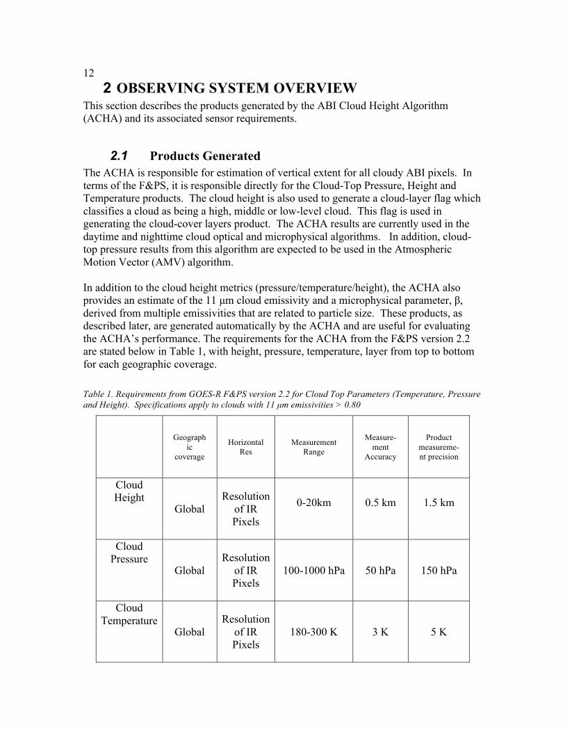
2.1 Products Generated The ACHA is responsible for estimation of vertical extent for all cloudy ABI pixels. In terms of the F&PS, it is responsible directly for the Cloud-Top Pressure, Height and Temperature products. The cloud height is also used to generate a cloud-layer flag which classifies a cloud as being a high, middle or low-level cloud. This flag is used in generating the cloud-cover layers product. The ACHA results are currently used in the daytime and nighttime cloud optical and microphysical algorithms. In addition, cloud-top pressure results from this algorithm are expected to be used in the Atmospheric Motion Vector (AMV) algorithm. In addition to the cloud height metrics (pressure/temperature/height), the ACHA also provides an estimate of the 11 µm cloud emissivity and a microphysical parameter, β, derived from multiple emissivities that are related to particle size. These products, as described later, are generated automatically by the ACHA and are useful for evaluating the ACHA’s performance. The requirements for the ACHA from the F&PS version 2.2 are stated below in Table 1, with height, pressure, temperature, layer from top to bottom for each geographic coverage. Table 1. Requirements from GOES-R F&PS version 2.2 for Cloud Top Parameters (Temperature, Pressure and Height). Specifications apply to clouds with 11 µm emissivities > 0.80

Geograph

ic coverage

Horizontal Res

Measurement Range

Measure-ment

Accuracy

Product measureme-nt precision

Cloud Height

Global Resolution

of IR Pixels

0-20km

0.5 km

1.5 km

Cloud Pressure

Global Resolution

of IR Pixels

100-1000 hPa 50 hPa 150 hPa

Cloud Temperature

Global Resolution

of IR Pixels

180-300 K 3 K 5 K

13 Furthermore, the GOES-R Series Ground Segment (GS) Project Functional and Performance Specification (F&PS) qualifies these requirements for cloudy regions with emissivities greater than 0.8 .

2.2 Instrument Characteristics The ACHA will operate on each pixel determined to be cloudy or probably cloud by the Cloud Mask. Table 2 summarizes the current channels used by the ACHA for the 9 modes it supports. Table 2. Channel numbers and wavelengths for the ABI Cloud Height Algorithm (ACHA). Symbols (i,j,k) refer to Equations 10-23.

MODIS Chan. #

AVHRR Chan#

VIIRS Chan #

Wavelength (µm)

ACHA Mode 1 2 3 4 5 6 7 8 9

27 n/a n/a 7.0 j k k 29 n/a 14 8.5 k 31 4 15 11.2 i i i i i i i i i 32 5 16 12.3 j j j j j 33 n/a n/a 13.3 j j k k

Note: Mode 9 is also used when fusion channel is available (See 3.4.2.10)

Table 3. ACHA Modes Supported by Sensor. (* = default mode)

Sensor Acha Modes Supported

AVHRR/1 1*

AVHRR/2 1,3*

AVHRR/3 1,3*

GOES I/M, MTSAT, COMS,FY-2 1,2,3,6*

GOES N/P 1,2,4,7*

GOES-R, AHI 1,2,3,4,5,6,7,8*

MODIS 1,2,3,4,5,6,7,8*

MSG/SEVIRI 1,2,3,4,6,7,8*

VIIRS 1,3,5*

AVHRR+HIRS, VIIRS+CrIS 9*

14 In general, the ACHA relies on the infrared observations to avoid discontinuities associated with the transition from day to night. ACHA performance is sensitive to imagery artifacts or instrument noise. Most important is our ability to accurately model the clear-sky values of the infrared absorption channels. The ability to perform the physical retrievals outlined in this document requires an accurate forward model, accurate ancillary data and well-characterized spectral response functions.

15 3 ALGORITHM DESCRIPTION

3.1 Algorithm Overview The ACHA serves a critical role in the GOES-R ABI processing system. It provides a fundamental cloud property but also provides information needed by other cloud and non-cloud algorithms. As such, latency was a large concern in developing the ACHA. The current version of the ACHA algorithm draws on the following heritage algorithms: ● The CLAVR-x split-window cloud height from NESDIS, and ● The MODIS CO2 cloud height algorithm developed by the UW/CIMSS. ● The GOES-R AWG 11/12/13.3 µm algorithm.

The ACHA derives the following cloud products (* = delivered as cloud CDR to NCDC): ● Cloud-top temperature*, ● Cloud-top pressure*, ● Cloud-top height*, and ● Quality flags*, ● Cloud 11 µm emissivity, ● Cloud microphysical index (β), ● Cloud optical depth, ● Cloud particle size, ● Cloud physical base height, ● Cloud physical top height

Section 3.4 describes the full set of outputs from the ACHA algorithm.

3.2 Processing Outline The processing outline of the ACHA is summarized in Figure 1. The current ACHA is implemented with the NOAA/NESDIS/STAR GOES-R AIT processing framework (FRAMEWORK). FRAMEWORK routines are used to provide all of the observations and ancillary data. The ACHA is designed to run on segments of data where a segment is comprised of multiple scan lines.

16

Figure 1 High level flowchart of the ACHA illustrating the main processing sections.

17 3.3 Algorithm Input

This section describes the input needed to process the ACHA. In its current configuration, the ACHA runs on segments comprised of 200 scan lines. While this is the ideal number of scan-lines per segment the ACHA algorithm should be run on, the algorithm does benefit from running on larger number of scan-lines. The ACHA must be run on arrays of pixels because spatial uniformity of the observations is necessary to the algorithm. In addition, the final algorithm design will include separate loops over those pixels in the segment determined to be local radiative centers (LRC), those pixels determined by the cloud typing algorithm to be single-layer clouds and those pixels determined to multi-layer clouds. The calculation of the LRC, which is done by the gradient filter, is described in the AIADD. The following sections describe the actual input needed to run the ACHA.

3.3.1 Primary Sensor Data The list below contains the primary sensor data used by the ACHA. By primary sensor data, we mean information that is derived solely from the ABI observations and geolocation information.

● Calibrated radiances for channels 14. ● Calibrated brightness temperatures for channels 14, 15 and 16. ● Cosine of sensor viewing zenith angle ● Satellite zenith angle ● Space mask ● Bad pixel mask for channels 14, 15, and 16

3.3.2 Ancillary Data The following lists the ancillary data required to run the ACHA. A more detailed description is provided in the AIADD. By ancillary data, we mean data that require information not included in the ABI observations or geolocation data. ● Surface elevation

● Surface Type

● NWP level associated with the surface

● NWP level associated with the tropopause

● NWP tropopause temperature

● Profiles of height, pressure and temperature from the NWP

● Inversion level profile from NWP

18 ● Surface temperature and pressure from NWP

● Viewing Zenith Angle bin

● NWP Line and element indices

● Clear-sky transmission, and radiance profiles for channels 14, 15 and 16

from the RTM

● Blackbody radiance profiles for channels 14, 15 and 16 from the RTM

● Clear-sky estimates of channel 14, 15 and 16 radiances from the RTM

3.3.3 Derived Data The following lists and briefly describes the data that are required by the ACHA that is provided by other algorithms. ● Cloud Mask

A cloud mask is required to determine which pixels are cloudy and which are not, which in turn determines which pixels are processed. This information is provided by the ABI Cloud Mask (ACM) algorithm. Details on the ACM are provided in the ACM ATBD.

● Cloud Type/Phase A cloud type and phase are required to determine which a priori information for the forward model are used. It is assumed that both the cloud type and phase are inputs to the ACHA algorithm. These products are provided by the ABI Cloud Type/Phase Algorithm. Information on the ABI Cloud Type/Phase is provided in the ABI Type/Phase ATBD.

● Local Radiative Centers

Given channel 14 (11µm) observed bright temperature, the local radiative center (LRC) is defined as the pixel location, in the direction of the gradient vector, upon which the gradient reverses. Practically, this starts with a 3 by 3 array surrounding a pixel, switches the center to the local maxima/minima in the array and initiate a new search. The gradient filter routine is required as an input to the ACHA. The original method to compute the gradient function is described in Pavolonis (2009) and in the AIADD. Some changes have been made to be used in ACHA. The required inputs to the gradient filter are:

o Calibrated brightness temperature at 11µm BT11, o The line and element size of the segment being processed, o The maximum search steps for local maxima/minima, o The upper and lower boundary values that the gradient must fall in

between to initiate the search,

19 o A flag for defining how the gradient reverses, i.e., when encountering a

local maximum (1) or minimum (-1), o A binary mask for the segment of cloudy pixels that have non-missing

BT11 for the segment, o The minimum and maximum valid BT11 values (220K and 290K

respectively).

The outputs from the gradient filter are the line and element of the LRC.

● Derived channel 14 top of troposphere emissivity The ACHA requires knowledge of the channel 14 emissivity of a cloud assuming that its top coincides with the tropopause. This calculation is done by using the measured channel 14 radiance, clear sky channel 14 radiance from the RTM, space mask, latitude/longitude cell index from the NWP, tropopause index from the NWP, viewing zenith angle bin index, and channel 14 µm blackbody radiance.

● Standard deviation of the channel 14 brightness temperature over a 3x3 pixel array.

● Standard deviation of the channel 14 – channel 15 brightness temperature difference over a 3x3 pixel array.

● Standard deviation of the channel 14 – channel 16 brightness temperature difference over a 3x3 pixel array.

3.4 Theoretical Description As described below, the ACHA represents an innovative approach that uses multiple IR channels within algorithm that provides results that are consistent for all viewing conditions. This approach combines multiple window channel observations with a single absorption channel observations to allow for estimation of cloud height without large assumptions on cloud microphysics for the first time from a geostationary imager. The remainder of this section provides the physical basis for the chosen approach.

3.4.1 Physics of the Problem The ACHA uses the infrared observations from the ABI to extract the desired information on cloud height. Infrared observations are impacted not only by the height of the cloud, but also its emissivity and how the emissivity varies with wavelength (a behavior that is tied to cloud microphysics). In addition, the emissions from the surface and the atmosphere can also be major contributors to the observed signal. Lastly, clouds often exhibit complex vertical structures that violate the assumptions of the single layer plane parallel models (leading to erroneous retrievals). The job of the ACHA is to exploit as much of the information provided by the ABI as possible with appropriate,

20 computationally efficient and accurate methods to derive the various cloud height products.

3.4.1.1 Motivation for ACHA Channel Selection The ACHA represents a merger of current operational cloud height algorithms run by NESDIS on the Polar Orbiting Environmental Satellite (POES) and GOES imagers. The current GOES-NOP cloud height algorithm applies the CO2 slicing method to the 11 and 13.3 µm observations. This method is referred to as the CO2/IRW approach. CO2 slicing was developed to estimate cloud-top pressures using multiple channels typically within the 14 µm CO2 absorption band. For example, the MODIS MOD06 algorithm (Menzel et al., 2006) employs four CO2 bands, and the GOES Sounder approach also employs four bands. CO2 slicing benefits from the microphysical simplicity provided by the spectral uniformity of the cloud emissivity across the 14 µm band. The GOES-NOP method suffers from two weaknesses relative to the MOD06 method. First, the assumption of spectral uniformity of cloud emissivity is not valid when applied to the 11 and 13.3 µm observations. Second, the 13.3 µm channel does not provide sufficient atmospheric opacity to provide the desired sensitivity to cloud height for optically thin high cloud (i.e., cirrus). For optically thick clouds, CO2 slicing methods rely simply on the 11 µm observation for estimating the cloud height. In contrast to the CO2/IRW approach used for GOES-NOP, the method employed operationally for the POES imager (AVHRR) uses a split-window approach based on the 11 and 12 µm observations. Unlike the 13.3 µm band, the 11 and 12 µm bands are in spectral windows and offer little sensitivity to cloud height for optically thin cirrus. As described in Heidinger and Pavolonis (2009), the split-window approach does provide accurate measurements of cloud emissivity and its spectral variation. Unlike the GOES-NOP imager or the POES Imager, the ABI provides the 13.3 µm CO2 channels coupled with multiple longwave IR windows (10.4, 11 and 12 µm). The ABI therefore provides an opportunity to combine the sensitivity to cloud height offered by a CO2 channel with the sensitivity to cloud microphysics offered by window channels and to improve upon the performance of the cloud height products derived from the current operational imagers. To demonstrate the benefits of the ACHA CO2/Split-Window algorithm, the sensitivity to cloud pressure offered by the channels used in the ACHA was compared to other channel sets using co-located MODIS and CALIPSO observations. These results where taken from Heidinger et al. (2010). Figure 2 shows a false color image from AQUA/MODIS for a cirrus scene observed on August 10, 2006 over the Indian Ocean. The red line in Figure 2 shows the location of the CALIPSO track. This scene is characterized by a predominantly single cirrus cloud of varying optical thickness with thicker regions on the left-side of the figure. An image of the 532 nm CALIPSO data for the trajectory shown in Figure 2 is shown in Figure 3.

21

Figure 2 A false color image constructed from 11 – 12µm BTD (Red), 4 – 11µm BTD (Green) and 11 µm BT reversed (Blue). Data are taken from AQUA/MODIS and CALIPSO/CALIOP on August 10, 2006 from 20:35 to 20:40 UTC. The red line is the CALIPSO track. In this color combination, cirrus clouds appear white but as the optical thickness increases, the ice clouds appear as light blue/cyan. Low-level water clouds appear as dark blue, and mid-level water clouds tend to have a red/orange color.

Figure 3 The 532 nm total backscatter from CALIOP along the red line shown in Figure 2. The grey line in the centre image is the Tropopause. In the work of Heidinger et al. (2009), an analysis was applied to the above data to study the impact on the cloud-top pressure solution space offered by various channel combinations commonly used on operational imagers. The term solution space refers to the vertical region in the atmospheric column where a cloud can exist and match the observations of the channels used in the algorithm. As described in Heidinger et al. (2009) this analysis was accomplished specifically by computing the emissivity profiles for each channel and determining the levels at which the emissivities were all valid and where the spectral variation of the emissivities was consistent with the chosen scattering

22 model. It is important to note that this analysis was not a comparison of algorithms, but a study of the impact of the pixel spectral information on the possible range of solutions. Figure 4 shows the resulting computation of the cloud-top pressure solution space spanned by the ACHA CO2/Split-Window algorithm (channels 14, 15 & 16). The grey area represents the region of the atmosphere where the MODIS observations of those channels were matched to within 0.5K. The blue points represent the cloud-top pressures where the cloud matched the MODIS observation most closely. In contrast, Figure 5 shows the same computation when using the VIIRS cloud-top height algorithm’s channel set. As described by Heidinger et al. (2009), the large improvement in the sensitivity to cloud top pressure seen in ACHA versus the VIIRS algorithm is due to the presence of the CO2 absorption channel. Because VIIRS offers only IR window channels, its ability to estimate the height of cirrus clouds with confidence is limited.

Figure 4 Cloud-top pressure solution space provided by the ACHA channel set for the ice clouds along the CALIPSO track for August 10, 2006 20:35 – 20:40 UTC. The grey lines represent the solution space provided by the selected GOES-R ABI channels. The black symbols provide the CALIOP cloud boundaries for the highest cloud layer. The blue points represent the location of the optimal cloud-top pressure solutions with this channel set. For clarity, only every fifth optimal cloud-top pressure solution is plotted.

23

Figure 5 Same as Figure 4 computed for the VIIRS channel set (3.75, 8.5, 11 and 12 µm). Red points show the MODIS (MYD06) results for reference.

3.4.1.2 Radiative Transfer Equation The radiative transfer equation (1) employed here is given as

(Eq. 1)

where Robs is the observed top-of-atmosphere radiance, Tc is the cloud temperature, B() represents the Planck Function and Rclr is the clear-sky radiance (both measured at the top of the atmosphere). Rac is the above-cloud emission; tac is the above-cloud transmission along the path from the satellite sensor to the cloud pixel. Finally, the cloud emissivity is represented by ec. All quantities in Eq. 1 are a function of wavelength, λ, and are computed separately for each channel. As described later, the 11 µm cloud emissivity is directly retrieved by the ACHA. The 12 and 13.3 µm cloud emissivities are not retrieved but they are utilized during the retrieval process. To account for the variation of ec with each channel, the β parameter is evoked. For any two-channel pair (1,2), the value of β can be constructed using the following relationship:

(Eq. 2)

24 Using this relationship, the cloud emissivities at 12 and 13 um can be derived from the cloud emissivity value at 11 µm as follows:

(Eq. 3)

(Eq. 4) For the remainder of this document, the value of ec will refer to the cloud emissivity at 11 µm and β will refer to the β(11/12µm) value unless stated otherwise. β is a convenient parameter because it also provides a direct link to cloud microphysics which is discussed in the next section. While the above radiative transfer equation is simple in that it assumes no scattering and that the cloud can be treated as a single layer, it does allow for semi-analytic derivations of the observations to the controlling parameters (i.e., cloud temperature). This behavior is critical because it allows for an efficient retrieval without the need for large lookup tables.

3.4.1.3 Cloud Microphysical Assumptions One of the strengths of the ACHA is that it allows cloud microphysics to vary during the retrieval process which should improve the cloud height estimates (Heidinger et al., 2009). Cloud microphysics is included in the retrieval through the spectral variation of the β parameters. The variation of β between different channel pairs is a function of particle size and ice crystal habit. For example, Parol et al. (1991) showed that β can be related to the scattering properties using the following relationship where ω is the single scattering albedo, g is the asymmetry parameter and σext is the extinction coefficient:

(Eq. 5) This relationship between β and the scattering properties will allow the ACHA to estimate cloud particle size from the retrieved β values. While the scattering properties for water clouds are well modeled by Mie theory, the scattering properties of ice clouds are less certain. To define a relationship between the β values for ice clouds, assumptions have to be made about the ice crystals. In the ACHA, we use the ice scattering models provided by Professor Ping Yang at Texas A&M University (Yang et al., 2005). In this database, ice models are separated by habits. To pick a habit, β values were computed using MODIS observations collocated with CALIPSO. We then compared how the observed β values corresponded with those computed from the scattering. The results indicated that aggregates modeled the

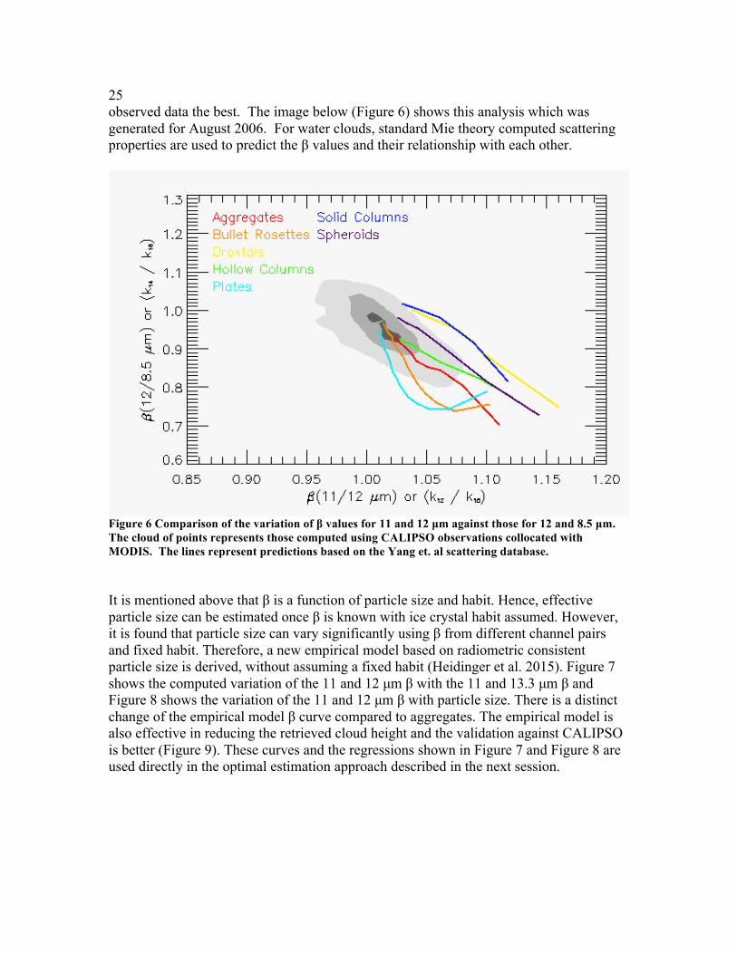
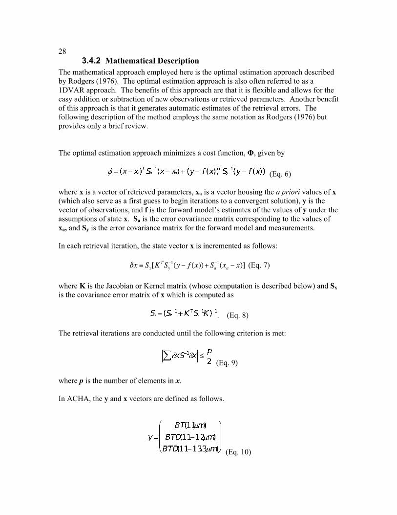
25 observed data the best. The image below (Figure 6) shows this analysis which was generated for August 2006. For water clouds, standard Mie theory computed scattering properties are used to predict the β values and their relationship with each other.

Figure 6 Comparison of the variation of β values for 11 and 12 µm against those for 12 and 8.5 µm. The cloud of points represents those computed using CALIPSO observations collocated with MODIS. The lines represent predictions based on the Yang et. al scattering database. It is mentioned above that β is a function of particle size and habit. Hence, effective particle size can be estimated once β is known with ice crystal habit assumed. However, it is found that particle size can vary significantly using β from different channel pairs and fixed habit. Therefore, a new empirical model based on radiometric consistent particle size is derived, without assuming a fixed habit (Heidinger et al. 2015). Figure 7 shows the computed variation of the 11 and 12 µm β with the 11 and 13.3 µm β and Figure 8 shows the variation of the 11 and 12 µm β with particle size. There is a distinct change of the empirical model β curve compared to aggregates. The empirical model is also effective in reducing the retrieved cloud height and the validation against CALIPSO is better (Figure 9). These curves and the regressions shown in Figure 7 and Figure 8 are used directly in the optimal estimation approach described in the next session.

26

Figure 7 Computed variation and linear-fit of the 11 and 13.3 µm β values to those computed using 11 and 12 µm. β is a fundamental measure of the spectral variation of cloud emissivity, and this curve is used in the forward model in the retrieval. The data shown are based on a radiometric consistent empirical model. For water clouds, Mie theory predicts a = -0.728 and b = 1.743.

27

Figure 8 Variation of the 11 and 12 µm β values as a function of the ice crystal radius for both the Empirical model and Aggregate Column model. This relation is used in the retrieval to produce an estimate of cloud particle size from the final retrieved β values.

Figure 9 Histogram showing differences between ACHA and CALIPSO cloud top height, using two ice models. One day of MODIS 5km data (06/30/2010) are run at mode 5 to simulate VIIRS output.

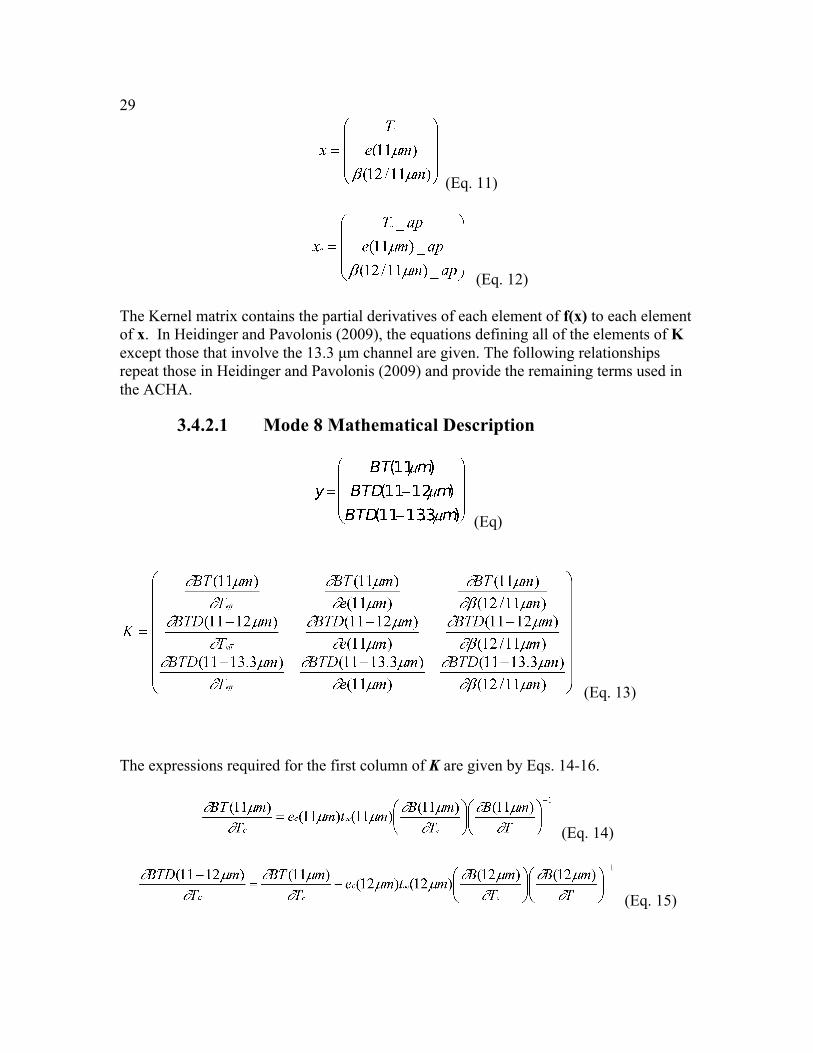
28 3.4.2 Mathematical Description

The mathematical approach employed here is the optimal estimation approach described by Rodgers (1976). The optimal estimation approach is also often referred to as a 1DVAR approach. The benefits of this approach are that it is flexible and allows for the easy addition or subtraction of new observations or retrieved parameters. Another benefit of this approach is that it generates automatic estimates of the retrieval errors. The following description of the method employs the same notation as Rodgers (1976) but provides only a brief review. The optimal estimation approach minimizes a cost function, Φ, given by

(Eq. 6)

where x is a vector of retrieved parameters, xa is a vector housing the a priori values of x (which also serve as a first guess to begin iterations to a convergent solution), y is the vector of observations, and f is the forward model’s estimates of the values of y under the assumptions of state x. Sa is the error covariance matrix corresponding to the values of xa, and Sy is the error covariance matrix for the forward model and measurements.

In each retrieval iteration, the state vector x is incremented as follows:

δx = Sx[K

TSy−1(y− f (x))+ Sa

−1(xa − x)] (Eq. 7) where K is the Jacobian or Kernel matrix (whose computation is described below) and Sx is the covariance error matrix of x which is computed as

. (Eq. 8)

The retrieval iterations are conducted until the following criterion is met:

(Eq. 9) where p is the number of elements in x. In ACHA, the y and x vectors are defined as follows.

(Eq. 10)

29

(Eq. 11)

(Eq. 12)

The Kernel matrix contains the partial derivatives of each element of f(x) to each element of x. In Heidinger and Pavolonis (2009), the equations defining all of the elements of K except those that involve the 13.3 µm channel are given. The following relationships repeat those in Heidinger and Pavolonis (2009) and provide the remaining terms used in the ACHA.

3.4.2.1 Mode 8 Mathematical Description

(Eq)

(Eq. 13)

The expressions required for the first column of K are given by Eqs. 14-16.

(Eq. 14)

(Eq. 15)

30

(Eq. 16)

The expressions for the second column of K are given by Eqs. 17-19.

(Eq. 17)

(Eq. 18)

(Eq. 19)

Finally, the derivative of each forward model simulation with respect to β(12/11µm) is given by the following equations:

(Eq. 20)

(Eq. 21)

(Eq. 22)

31

The values of are computed using the regression shown in Figure 7. For water clouds, the same form of a regression shown in Figure 7 is used except that the a-coefficient is -0.728 and the b-coefficient is 1.743.

3.4.2.2 Estimation of Prior Values and their Uncertainty The proper implementation of ACHA requires meaningful estimates of a priori values housed in xa and their uncertainties housed in Sa. Sa is a two-dimensional matrix with each dimension being the size of xa. For the ACHA, we assume Sa is a diagonal matrix with each element being the assumed variance of each element of xa as illustrated below.

(Eq. 23)

In the ACHA, we currently use the a priori estimate of xa and Sa based on phase and 11µm properties, as well as from calipso values as reported by Heidinger and Pavolonis (2009). For water typed clouds, the a priori values of Tc use 11 µm brightness temperature at the LRC, and emissivities are computed from an a priori estimate of optical thickness and satellite zenith angle: εc_ ap(water) =1.0− exp(−τ _ ap_water /mu) (Eq. 24) where a value of 3.0 is use for τ _ ap(water) , and mu is cosine of satellite zenith angle. Fixed values of 10 K and 0.1 are used for the values of σ 2

. For ice type clouds, the a priori values and σ 2 of Tc and emissivity are computed as follows: Tc_ ap(ice) = εc_weight *BT11_ LRC + (1.0−εc_weight)*(T _ tropo+Tc_offset _ cirrus)σ 2 (Tc)_ ap(ice) = εc_weight *Tc_uncer _opaque+ (1.0−εc_weight)*Tc_uncer _ cirrusεc_ ap(ice) = εc_weightσ 2 (εc)_ ap(ice) = 0.4

(Eq. 25)

where εc_weight is the 11 µm emssivity at tropopause, T_tropo is the temperature at tropopause, and the values for Tc_offset_cirrus, Tc_uncer_opaque and Tc_uncer_cirrus are 15K, 10K and 20K.

32 The a priori values of β are taken from scattering theory and are set to 1.06 for ice-phase clouds and 1.3 for water-phase clouds. The standard deviation of β is assumed to be 0.2 based on the distributions of Heidinger and Pavolonis (2009). Table 4 provides the current a priori and uncertainty values used in ACHA. Table 4: The a priori (first guess) retrieval values used in the ACHA retrieval.

Cloud Type Tc σ2(Tc) ε σ2 (ε) β σ2 (β) Fog BT11_LRC 10 K εc_ ap(water) 0.1 1.3 0.2 Water BT11_LRC 10 K εc_ ap(water) 0.1 1.3 0.2 Supercooled BT11_LRC 10 K εc_ ap(water) 0.1 1.3 0.2 Mixed BT11_LRC 10 K εc_ ap(water) 0.1 1.3 0.2 Thick Ice Tc_ap(ice) σ 2 (Tc)_ ap(ice)

εc_ ap(ice) 0.4 1.06 0.2

Cirrus Tc_ap(ice) σ 2 (Tc)_ ap(ice)

εc_ ap(ice) 0.4 1.06 0.2

Multi-layer Tc_ap(ice) σ 2 (Tc)_ ap(ice)

εc_ ap(ice) 0.4 1.06 0.2

3.4.2.3 Estimation of Forward Model Uncertainty This section describes the estimation of the elements of Sy which contain the uncertainty expressed as a variance of the forward model estimates. Sy is assumed be a symmetric matrix. Both diagonal and off-diagonal components are computed. Assumed to be symmetric, Sy can be expressed as follows:

Sy =

σ BT (11µm)2 σ covBT (11,12µm)

2 σ covBT (11,13µm)2

σ covBT (11,12µm)2 σ BTD(11−12µm)

2 σ covBT (12,13µm)2

σ covBT (11,13µm)2 σ covBT (1213µm)

2 σ BTD(11−133µm)2

"

#

$$$$

%

&

''''

(Eq. 26)

The diagonal variance terms are computed by summing up three components:

σ diag

2 =σ instr2 +[1− ec (11µm)]

2σ clr2 +σ hetero

2 (Eq. 27) The first component (σ2

instr) represents instrument noise and calibration uncertainties. The second component represents uncertainties caused by the clear-sky radiative transfer (σclear). σclear is assumed to decrease linearly with increasing ec. For opaque clouds, the uncertainties associated with clear-sky radiative transfer are assumed to be negligible.

33 Due to the large variation in NWP biases on land and ocean, separate land and ocean uncertainties are assumed. The third component (σhetero) is the term that accounts for the larger uncertainty of the forward model in regions of large spatial heterogeneity. Currently, the ACHA uses the standard deviation of each element of y computed over a 3x3 pixel array as the value of σhetero. The off diagonal variance terms are expressed in a simpler way: σ off −diag

2 = [1− ec (11µm)]2σ clr

2 (11,12 /13µm) (Eq. 28)

3.4.2.4 Estimation of Quality Flags and Errors One of the benefits of the 1DVAR approach is the diagnostic terms it generates automatically. If the values of Sa, Sy and K are properly constructed, the values of Sx should provide an estimate of the uncertainties of the retrieved parameters, x. The diagonal term of Sx provides the uncertainty expressed as a variance of each parameter. While these estimates are useful, the current ACHA also generates a 4-level quality flag. The integer quality flags are determined by the relative values of the diagonal terms of Sx and Sa. If the estimated uncertainty in a element of x is less than one third of the prescribed uncertainty of the corresponding element of xa, a parameter quality indicator, which is not the product quality flag described in section 3.4.3.3, of 3 is assigned. Similarly a parameter quality indicator of 2 is assigned for pixels where the estimated uncertainty of x lies between one third and two thirds of the uncertainty of the corresponding element of xa. Values with higher uncertainties are given a parameter quality indicator of 1. Retrievals that do not converge are given a parameter quality indicator of 0. A description of the parameter quality indicator is in section 3.4.3.2.

3.4.2.5 Impact of Local Radiative Center Pixels As discussed above, the first pass through the retrieval occurs for those pixels determined to be local radiative centers which physically correspond to local maxima in cloud opacity. The full pixel processing order is described below. The objective is to first apply the retrieval to the more opaque pixels and to use this information for the less opaque pixels. In the ACHA, the a priori value of Tc for pixels that have local radiative centers identified for them are assumed to be the values of Tc estimated for the local radiative centers. The uncertainty values of the forward model remain those given in Table 5. Table 5: Values of uncertainty for the forward model used in the ACHA retrieval.

Element of f σinstr σclear (Ocean) σclear (Land) T(11um) 1.0 1.5 5.0

BTD(11 – 12µm) 1.0 0.5 1.0 BTD(11 – 13µm) 2.0 4.0 4.0

34 3.4.2.6 Treatment of Multi-layer Clouds

For pixels determined to be multi-layer clouds, the lower boundary condition is assumed to be a lower cloud and not the surface of the earth. With this assumption, the forward model remains unchanged when treating multi-layer clouds. As discussed by Heidinger and Pavolonis (2009), the mean height of water clouds determined from MODIS is 2 km above the surface. Therefore, for all multi-layer pixels, the lower boundary condition is assumed to be an opaque cloud situated 2 km above the surface of the earth. The same equations apply except that the clear-sky observations are recomputed to reflect the change in the lower boundary condition. It is a goal for future versions of this algorithm to dynamically compute the height/temperature of the lower cloud layer in multi-layer situations. In the ACHA, information about the height of the surrounding low clouds is used to estimate the height of low clouds underneath higher clouds in detected multi-layer situations. Figure 10 provides a visual aid for understanding this process. In this example, assume that the ABI pixel observed above Low Cloud #3 is correctly identified as a multi-layer cloud by the ABI cloud typing algorithm. Also, assume that Low Clouds #1 and #5 are correctly identified as low clouds and have successful cloud height solutions from the ACHA. The ACHA uses the height information for Low Clouds #1 and #5 to estimate the height of Low Cloud #3 instead of assuming a fixed height of all low clouds detected below high clouds. This computation is accomplished by taking the mean of all low cloud pressures that surround the multi-layer cloud pixel within a NxN box. Currently, the size of the box (N) is set to 11. If no low cloud results are found within the NxN box, a default value of the cloud pressure is used. This default value is 200 hPa lower than the surface pressure. The application of this logic requires that the low cloud information be available before processing the multi-layer pixels. This logic is described in the next section.

Figure 10 Schematic illustration of multi-layer clouds.

35 3.4.2.7 Pixel Processing Order with the ACHA

As stated above, applying the multi-layer logic and applying local-radiative center logic require that some pixels be processed before others. In this section, we describe this logic. The pixel processing order in the ACHA is as follows:

1. Single-layer Radiative Centers, 2. Non-local radiative center water clouds, 3. Multi-layer clouds, and 4. All remaining unprocessed cloudy pixels.

Pixels that are single-layer radiative centers can be done first since they rely not on the results of other pixels. Pixels that are single-layer water clouds can then be processed because they would be influenced by the pixels that are single layers and radiative centers. Single-layer ice pixels cannot be processed yet since they may require knowledge of the multi-layer results if their LRC computation points to a multi-layer pixel. The next pixels that can be processed are the multi-layer pixels. After this computation, all remaining pixels can be processed.

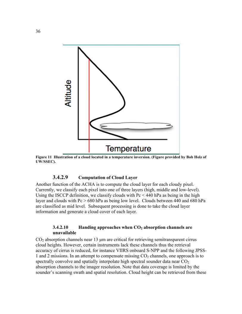
3.4.2.8 Computation of Cloud Height and Cloud Pressure Once Tc is computed, the NWP temperature profiles are used to interpolate the values of cloud-top pressure, Pc, and cloud-top height, Zc. Two separate methods are applied depending on whether the cloud is in an inversion or not. An inversion is defined as a region in the atmosphere where the temperature increases with height. Figure 11 provides an illustration of an inversion. When a cloud temperature is found to reside outside of an inversion, a simple linear interpolation is used to estimate cloud-top pressure and height. In the presence of inversions, the monotonic relationship between temperature and pressure/height disappears and a single value of cloud temperature can correspond to multiple pressure or height values. Atmospheric inversions are common at low levels over the ocean. This issue plagues all infrared cloud height algorithms including those employed by the MODIS and GOES sounder teams. The presence of low-level inversions is determined by analysis of the NWP temperature profile. Currently, if any layer below 700 hPa and 50 hPa above the surface is found to be warmer than the layer below it, the clouds are assumed to reside in an inversion as illustrated in Figure 11. In this case, the cloud height is estimated by dividing the difference (DeltaT) between the cloud temperature and the surface temperature by a predefined lapse rate. Currently, the lapse rate is assumed to be a polynomial function of DeltaT. The vertical resolution of NWP profiles is not sufficient to use them directly in the presence of inversions. This procedure is only implemented over water surfaces and for water-phase clouds. It is important to note that this issue requires further study. The Cloud Application Team is working with the AMV team and other cloud remote sensing groups to determine an optimal strategy when inversions are present.

36

Figure 11 Illustration of a cloud located in a temperature inversion. (Figure provided by Bob Holz of UW/SSEC).

3.4.2.9 Computation of Cloud Layer Another function of the ACHA is to compute the cloud layer for each cloudy pixel. Currently, we classify each pixel into one of three layers (high, middle and low-level). Using the ISCCP definition, we classify clouds with Pc < 440 hPa as being in the high layer and clouds with Pc > 680 hPa as being low level. Clouds between 440 and 680 hPa are classified as mid level. Subsequent processing is done to take the cloud layer information and generate a cloud cover of each layer.

3.4.2.10 Handing approaches when CO2 absorption channels are unavailable

CO2 absorption channels near 13 µm are critical for retrieving semitransparent cirrus cloud heights. However, certain instruments lack these channels thus the retrieval accuracy of cirrus is reduced, for instance VIIRS onboard S-NPP and the following JPSS-1 and 2 missions. In an attempt to compensate missing CO2 channels, one approach is to spectrally convolve and spatially interpolate high spectral sounder data near CO2 absorption channels to the imager resolution. Note that data coverage is limited by the sounder’s scanning swath and spatial resolution. Cloud height can be retrieved from these

37 data, such as from the CO2 slicing method, which at a coarser spatial resolution yet provide a valuable additional priori value for cirrus clouds. Revisions are made to the a priori value of cloud temperature and the associated background error variance matrix element to reflect the information from the sounder: x0 (1) = [x0s (1) / Sas (1,1)+ x0i (1) / Sai (1,1)] / (1 / Sas (1,1)+1/ Sai (1,1))Sa (1,1) = [1 / Sas (1,1)+1/ Sai (1,1)]

−1 (Eq. 29)

where x0s and x0i stand for the a-priori values from sounder and imager, respectively, and similarly for Sa . This approach benefits from both the sounder’s spectral information and imager’s high spatial resolution. Meanwhile, it preserves the integrity of the OE approach without fundamental modifications. The other approach is called the “FUSION” method. Unlike the previous approach, this generates a 13.3 µm BT based on a statistical reconstruction method (Cross et al. 2013) with no gaps. This is treated as mode 9 in ACHA option, separate from mode 8 when 13.3 µm is regularly available from the imager.

3.4.2.11 IR Cloud Optical Properties ACHA generates IR based optical properties, including cloud optical depth and effective particle size. The IR based retrieval are very sensitive to thin optical depth and small particle size compared to daytime solar reflectance based bispectral method. Plus, it provides consistent day and night retrievals. As discussed in 3.4.1.3, the microphysical parameter β and particle size can be parameterized by a polynomial relationship. Since β is an ACHA output, particle size can be obtained from pre-computed coefficients. Subsequently, scattering properties in Eq. (5) can be determined from particle size using similar polynomial relationship. The next step is to estimate optical depth. The absorption optical depth τabs can be estimated from cloud emissivity ec:

𝜏!"# =  −𝜇  𝑙𝑛 1− 𝑒! (Eq. 30) where µ is the cosine of the viewing zenith angle. The full optical depth at visible wavelength is derived by

τ vis =σ vis

σ 11µm

τ abs1−ω11µmg11µm

(Eq. 31)

38 3.4.3 Algorithm Output

3.4.3.1 Output The output of the ACHA provides the following ABI cloud products listed in the F&PS: ● Cloud-top temperature, ● Cloud-top pressure, ● Cloud-top height, and ● Cloud cover layer.

All of these products are derived at the pixel level for all cloudy pixels. Example images of the above products are provided in Section 4.2.

3.4.3.2 Intermediate data The ACHA derives the following intermediate products that are not included in F&PS, but are used in other algorithms, such as the atmospheric motion vector (AMV) algorithm: ● Error estimates, ● Cloud 11 µm emissivity, and ● Cloud microphysical index (β). ● Cloud base height ● IR retrieved cloud optical depth ● IR retrieved cloud particle size ● Optimal estimation cost function ● Parameter Quality Indicator

The Parameter Quality Indicator is a discretized and normalized version of the error estimates. It is not a substitute for the product quality flag (see below). A detailed description of the parameter quality indicator is provided in section 3.4.2.4.

3.4.3.3 Product Quality Flag In addition to the algorithm output, a pixel level product quality flag will be assigned. The possible values are as follows:

Flag Value Description 0 No retrieval attempted 1 Retrieval attempted and failed 2 Marginally successful retrieval 3 Fully successful retrieval

39 3.4.3.4 Processing Information Flag

In addition to the algorithm output and quality flags, processing information, or how the algorithm was processed, will be output for each pixel. If the bit is 0, then the answer is no, and if the bit is 1, the answer is yes.

Bit Description 1 Cloud Height Attempted 2 Bias Correction Employed 3 Ice cloud retrieval 4 Local Radiative Center Processing Used 5 Multi-layer Retrieval 6 Lower Cloud Interpolation used 7 Boundary Layer Inversion Assumed 8 NWP Profile Inversion Assumed

3.4.3.5 Metadata In addition to the algorithm output, the following will be output to the file as metadata for each file: ● Mean, Min, Max and standard deviation of cloud top temperature; ● Mean, Min, Max and standard deviation of cloud top pressure; ● Mean, Min, Max and standard deviation of cloud top height; ● Number of QA flag values ; ● For each QA flag value, the following information is required:

o Number of retrievals with the QA flag value, o Definition of QA flag, o Total number of detected cloud pixels, and o Terminator mark or determination.

40 4 Test Datasets and Outputs

4.1 Proxy Input Datasets S-NPP VIIRS data are available at the time of writing this ATBD. However, MODIS data are used instead as proxy data for two reasons. First, MODIS is recognized as a successful project, so validating again MODIS MYD06 product is critical to test ACHA performance across sensors. MODIS has the needed channel information (8.5, 11 and 12 µm) for ACHA run on VIIRS mode. By using MODIS as proxy data, the convenience of direct comparisons among MYD06, ACHA MODIS and ACHA VIIRS are possible without making collocation. Second, by using 5-km reduced resolution MODIS data, compared to 750m moderate resolution S-NPP VIIRS data, the retrievals and comparisons can be done in a relative fast way without compromising data integrity. As described below, the data used to test the ACHA are from Aqua MODIS observations on January 1, 2013 collocated with CALIPSO data. ACHA is run on mode 8, which is the default mode for MODIS. Additionally, run on mode 5 is conducted to mimic the VIIRS sensor as discussed in Table 3. The rest of this section describes the proxy and validation datasets used in assessing the performance of the ACHA.

4.1.1 MODIS Data MODIS provides 36 spectral channels with a spatial resolution of 250 m (band 1-2), 500 m (band 3-7) and 1000 m (band 8-36). MODIS provides an adequate source of proxy data for testing and developing the ACHA. One day Aqua 5-km resolution MODIS level 2 data from January 1, 2013 were generated from two ACHA modes and collocated information with CALIPSO is saved, and global subset level2b data in 0.1 degree resolution are also generated. The Aqua MODIS data were provided by the UW/SSEC Data Center and processed for the datasets specified in section 4.1.

4.1.2 CALIPSO Data With the launch of CALIPSO and CloudSat into the NASA EOS A-Train in April 2006, the ability to conduct global satellite cloud product validation increased significantly. Currently, CALIPSO cloud layer results are being used to validate the cloud height product of the ACHA. The CALIPSO data used here are the 1 km cloud layer results. Fig. 12 shows an example of CALIPSO profiles used in this study.

41

Figure 12 Illustration of CALIPSO data used in this study. Top image shows a 2D backscatter profile. Bottom image shows the detected cloud layers overlaid onto the backscatter image. Cloud layers are colored magenta. (Image courtesy of Michael Pavolonis, NOAA)

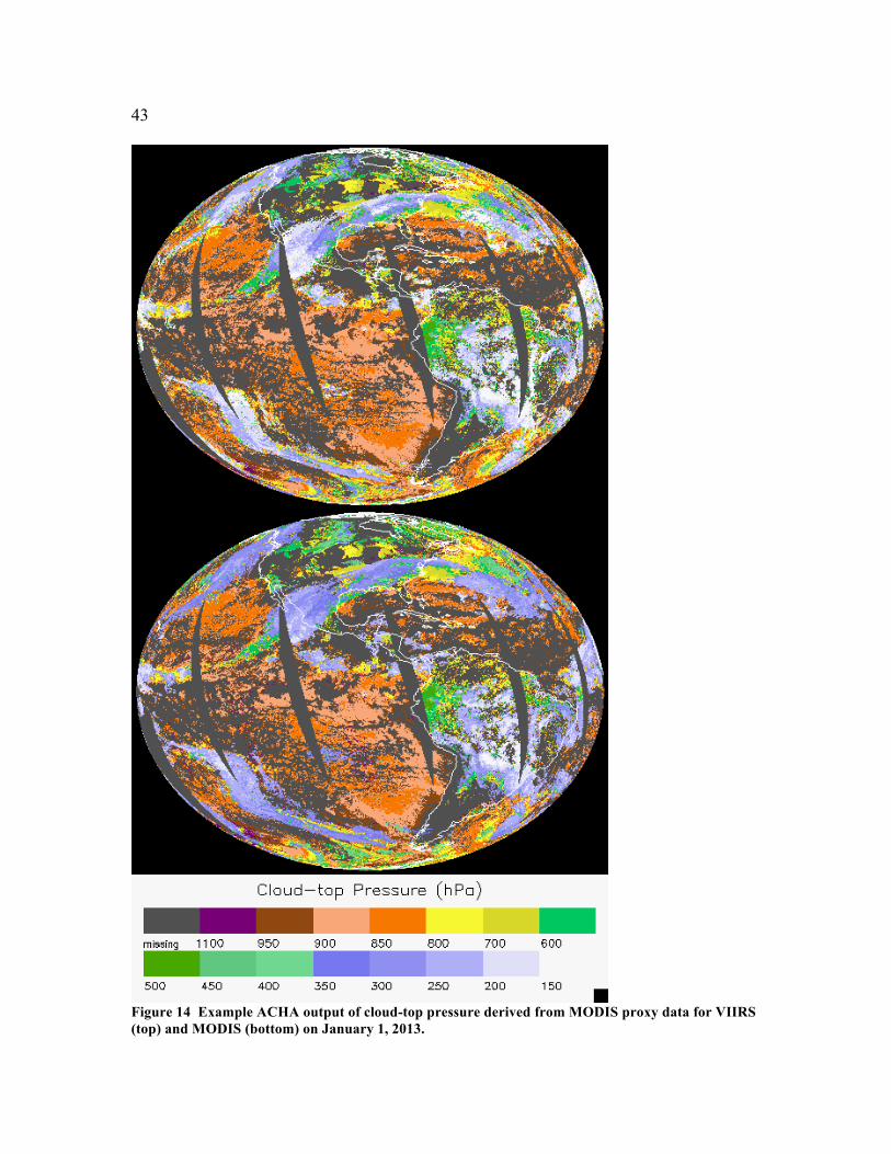
4.2 Output from Simulated/Proxy Inputs Datasets The ACHA result was generated using the MODIS data from the dataset specified in section 4.1. During both the TRR and subsequent tests, comparisons between the online and offline (Cloud AWG) output of the ACHA, when the same inputs were used, showed an exact match of the height, temperature and pressure outputs. These tests were conducted under different conditions using the same input for both the online and offline tests. Figures 13-17 shown below illustrate the ACHA cloud-top temperature, pressure, height, cloud layer and cloud emissivity. These images correspond to global ascending tracks on January 1, 2013 and top and bottom images correspond to VIIRS and MODIS ACHA modes respectively.

42

Figure 13 Example ACHA output of cloud-top temperature derived from MODIS proxy data for VIIRS (top) and MODIS (bottom) on January 1, 2013.

43

Figure 14 Example ACHA output of cloud-top pressure derived from MODIS proxy data for VIIRS (top) and MODIS (bottom) on January 1, 2013.

44

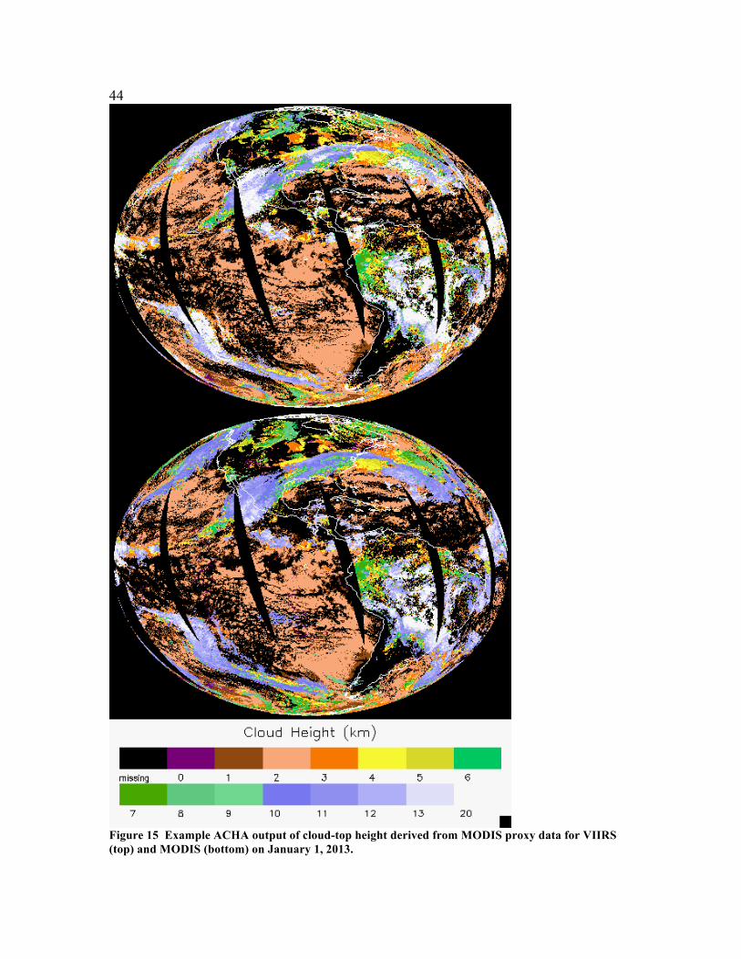
Figure 15 Example ACHA output of cloud-top height derived from MODIS proxy data for VIIRS (top) and MODIS (bottom) on January 1, 2013.

45

Figure 16 Example ACHA output of cloud layer derived from MODIS proxy data for VIIRS (top) and MODIS (bottom) on January 1, 2013.

46

Figure 17 Example ACHA output of 11 µm cloud emissivity derived from MODIS proxy data for VIIRS (top) and MODIS (bottom) on January 1, 2013.

47 4.2.1 Precisions and Accuracy Estimates

To estimate the precision and accuracy of the ACHA, CALIPSO data from NASA EOS A-Train are used. This new data source provides unprecedented information on a global scale. While surface based sites provide similar information, the limited sampling they offer requires years of analysis to generate the amount of collocated data provided by CALIPSO in a short time period.

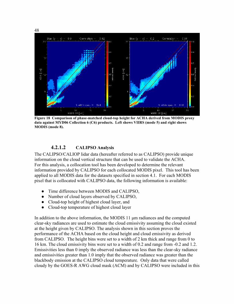
4.2.1.1 MODIS Analysis The MODIS cloud height products (MYD06) have proven to be a useful and accurate source of information to the cloud remote sensing community. The MYD06 cloud height algorithm employs the longwave CO2 channels in a CO2 slicing approach to estimate the cloud-top pressure and cloud effective cloud amount. More details on this algorithm are available in the MODIS MYD06 ATBD (Menzel et al., 2006). The MODIS MYD06 ATBD quotes the cloud-top pressure accuracy to be roughly 50 mb, which is under the GOES-R ABI specification of 100 mb. Given the wide use of the MYD06 product set, a comparison between the ACHA and MYD06 is warranted. While the MYD06 product set does provide the direct measure of cloud height provided by CALIPSO, it does complement the verification by providing qualitative comparisons over a larger domain. Given the availability of the longwave CO2 channels on MODIS, we expect MYD06 to provide superior results especially for semitransparent cirrus. It is also assumed that cloud products should only agree when the cloud detection and phase results agree. An example of this comparison is shown in Figure 18. In this figure, the global ascending track cloud-top height data in 0.1 degree resolution for January 1, 2013 as shown above are compared on a phase-matched basis. The left panels shows the comparison for ACHA VIIRS against MYD06 and right for ACHA MODIS. The results indicate that the height differences between ACHA and MYD06 are less than 1km and the correlations are above 0.9. Although comparing two passive satellite measurements cannot be thought of as validation, the bias and precision estimates of the ACHA relative to MODIS indicate the AWG algorithm is performing well. The cloud-top height comparison also shows that the ACHA algorithm is meeting specification relative to MODIS for this scene.

48

Figure 18 Comparison of phase-matched cloud-top height for ACHA derived from MODIS proxy data against MYD06 Collection 6 (C6) products. Left shows VIIRS (mode 5) and right shows MODIS (mode 8).

4.2.1.2 CALIPSO Analysis The CALIPSO/CALIOP lidar data (hereafter referred to as CALIPSO) provide unique information on the cloud vertical structure that can be used to validate the ACHA. For this analysis, a collocation tool has been developed to determine the relevant information provided by CALIPSO for each collocated MODIS pixel. This tool has been applied to all MODIS data for the datasets specified in section 4.1. For each MODIS pixel that is collocated with CALIPSO data, the following information is available: ● Time difference between MODIS and CALIPSO, ● Number of cloud layers observed by CALIPSO, ● Cloud-top height of highest cloud layer, and ● Cloud-top temperature of highest cloud layer

In addition to the above information, the MODIS 11 µm radiances and the computed clear-sky radiances are used to estimate the cloud emissivity assuming the cloud existed at the height given by CALIPSO. The analysis shown in this section proves the performance of the ACHA based on the cloud height and cloud emissivity as derived from CALIPSO. The height bins were set to a width of 2 km thick and range from 0 to 16 km. The cloud emissivity bins were set to a width of 0.2 and range from -0.2 and 1.2. Emissivities less than 0 imply the observed radiance was less than the clear-sky radiance and emissivities greater than 1.0 imply that the observed radiance was greater than the blackbody emission at the CALIPSO cloud temperature. Only data that were called cloudy by the GOES-R AWG cloud mask (ACM) and by CALIPSO were included in this

49 analysis. Figure 19 shows the relative distribution of pixels in Zc-ec space for this analysis. Any cells that are colored dark did not have enough points for analysis.

Figure 19 Relative distribution of points used in the validation of the ACHA applied to MODIS data for data observed during simultaneous MODIS and CALIPSO periods on January 1, 2013.

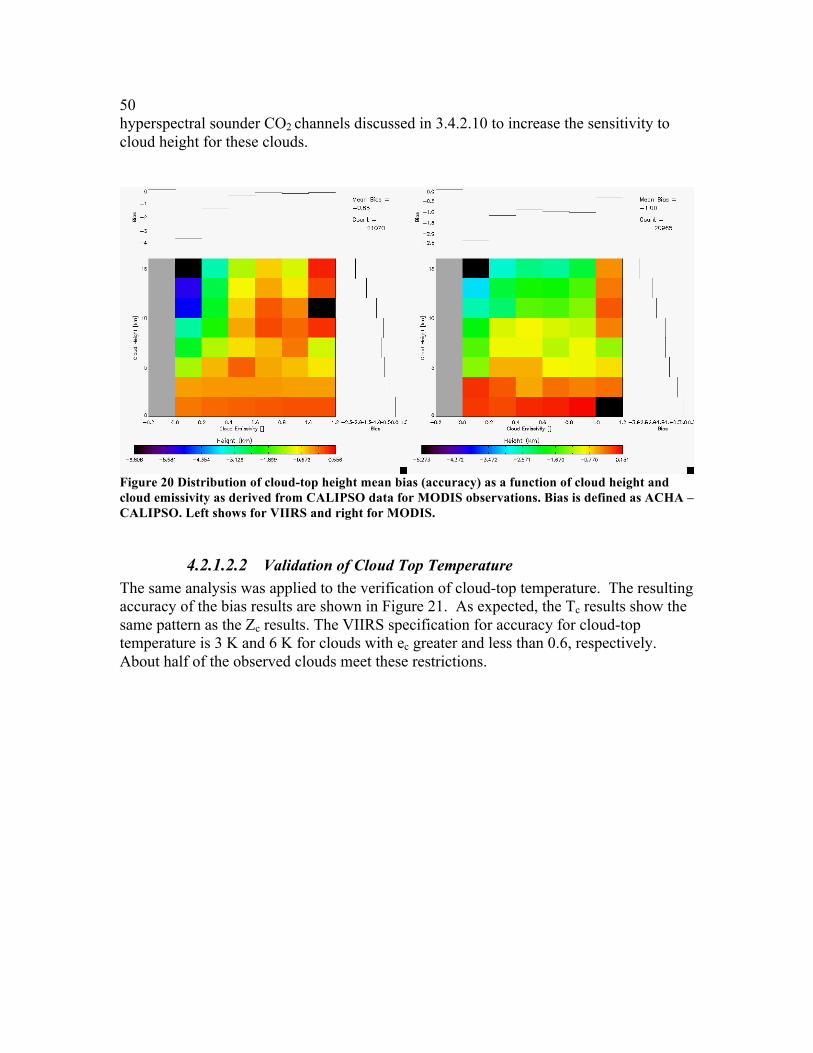
4.2.1.2.1 Validation of Cloud Top Height For each Zc – ec bin, the mean bias in the ACHA – CALIPSO results was compiled. The mean bias is the accuracy. The resulting distributions of the mean of the bias is shown in Figure 20 for both VIIRS and MODIS. The VIIRS specification for accuracy is 1 km for clouds with ec > 0.6 and 2 km when ec < 0.6. While the accuracy is below this value for nearly all stated cloudiness stratifications, there is exception for VIIRS high clouds, in particular optical thin cirrus. This is primarily due to missing LW CO2 absorption channels. Work is being done to improve in this area as well and involves incorporating radiance biases to improve our ability to reproduce the cirrus observations and use of the

50 hyperspectral sounder CO2 channels discussed in 3.4.2.10 to increase the sensitivity to cloud height for these clouds.

Figure 20 Distribution of cloud-top height mean bias (accuracy) as a function of cloud height and cloud emissivity as derived from CALIPSO data for MODIS observations. Bias is defined as ACHA – CALIPSO. Left shows for VIIRS and right for MODIS.

4.2.1.2.2 Validation of Cloud Top Temperature The same analysis was applied to the verification of cloud-top temperature. The resulting accuracy of the bias results are shown in Figure 21. As expected, the Tc results show the same pattern as the Zc results. The VIIRS specification for accuracy for cloud-top temperature is 3 K and 6 K for clouds with ec greater and less than 0.6, respectively. About half of the observed clouds meet these restrictions.

51

Figure 21 Distribution of cloud-top temperature mean bias (accuracy) as a function of cloud height and cloud emissivity as derived from CALIPSO data for MODIS observations. Bias is defined as ACHA – CALIPSO. Left shows for VIIRS and right for MODIS.

4.2.1.2.3 Validation of Cloud Top Pressure The current suite of CALIPSO products does not include pressure as a product. We are modifying our tools to estimate cloud pressure from the cloud height products in the CALIPSO product suite. However, the cloud-top pressure errors are highly correlated to the cloud-top height errors shown above. The comparisons to MODIS confirm this correlation.

4.2.1.2.4 Validation of Cloud Layer The cloud layer product has been defined as a flag that indicates where a cloud-top falls into 3 discrete vertical layers in the atmosphere. These layers are defined as follows: ● Low: pressures between the surface and 680 hPa, ● Mid: pressures between 680 and 44 hPa, and ● High: pressures lower than 440 hPa.

These layers are the standard layers used in many cloud product systems such as those used in the International Satellite Cloud Climatology (ISCCP). Cloud amounts in these layers have often been used for verifying cloud parameterization in NWP forecasts. As mentioned above, CALIPSO does not generate a standard cloud-top pressure product so direct validation of the cloud layer product using CALIPSO is not possible. However, CALIPSO does generate a product whereby the low layer is defined as clouds with top

52 heights less than 3.25 km, the mid layer is defined as clouds with tops between 3.25 and 6.5 km and the high layer is defined as cloud with tops higher than 6.5 km. These height layers roughly correspond to the pressure layers used to define the VIIRS product. At preparation of this ATBD for VIIRS, there is no direct comparison of VIIRS layers and CALIPSO. However, we previously conducted a comparison based on simulated ABI cloud product. Using the CALIPSO layer height definitions, a height-based layer can be derived from the ABI cloud-top heights. In addition, the CALIPSO cloud-top heights of the highest layer can be computed into height-based layer flags. When the CALIPSO and ABI height-based cloud layer flags are compared, a POD value of 91.4 % is computed. The data used in this comparison are the 10-week of SEVIRI runs to simulate ABI. This level of agreement indicates the ABI cloud layer product meets its accuracy specification of 80%. At this time, there is no precision specification placed on this product.

4.2.1.2.5 Validation of IR Cloud Optical Properties IR retrieved Cloud optical properties have also been validated against different data sources, as shown in Figures 22 and 23 below. An additional validation source from CALIPSO/IIR is included. Note that IR cloud product shown here is not from direct ACHA output. Instead, it is computed from MYD06 emissivity product and physically and quantitatively similar as variables from ACHA. The figures are adapted from Heidinger et al. (2015). The results indicate that both cloud optical depth and effective particle size are consistent with existing validation datasets. Therefore, these ACHA product can serve as a reliable dataset for thin cirrus study at both day and night conditions.

53

Figure 22 Comparison of the cloud optical depth retrievals. Top panel compares to the CALIPSO/CALIOP, middle panel compares to the C6 MYD06 retrievals, and bottom panel compares to CALIPSO/IIR.

54

Figure 23 Comparison of the cloud effective radius retrievals. Top panels compare to the C6 MYD06 retrieval, and bottom panel compare to CALIPSO/IIR.

4.2.2 Error Budget Using the validation described above, the following table provides our preliminary estimate of an error budget. The “Bias Estimate” column values most closely match our interpretation of the F&PS accuracy specifications. To match the F&PS, these numbers were generated for low-level clouds with emissivities greater than 0.8. Cloud pressure errors were estimated assuming 1000m = 100 hPa which is a good approximation at low levels.

55 Table 6. Preliminary estimate of error budget for ACHA.

Product Accuracy and Precison

Specification (VIIRS)

Bias Estimate

Standard Deviation Estimate

Cloud-top Temperature 3K when τ ≥ 1, 6K when τ < 1 0.95 K 3.65 K

Cloud-top Height 1km when τ ≥ 1, 2km when τ < 1 0.41 km 0.75 km

Cloud-top Pressure

τ ≥ 1: 100mb for [0,3km], 75mb for [3,7km], 50mb

for > 7km

-22.6 hPa 47.0 hPa

As Table 6 shows, the ACHA meets the 100% VIIRS requirements for precision and accuracy. It is important to identify the three main drivers of the ACHA error budget.

1. Lack of Knowledge of Low-level Inversions. The current F&PS specifications demand accurate performance of cloud height for low-level clouds. Even if the instrument and retrievals are perfect and an accurate cloud-top temperature is estimated, the unknown effects of inversions can result in cloud heights failing to meet specification.

2. Characterization of Missing CO2 Channel. Our ability to place cirrus properly is in large part determined by our ability to model the observations within CO2 absorption bands. By including sounder (CrIS) information, we have shown success in better placing cirrus cloud heights. With these information, the ability to perform well in the presence of cirrus clouds is in jeopardy.

3. Multi-layer clouds. While the AWG cloud type algorithm does include a multi-layer detection, our knowledge of the properties of that lower cloud is limited.

The Cloud Application Team will continue to be involved in developments that impact the above error sources.

5 PRACTICAL CONSIDERATIONS

5.1 Numerical Computation Considerations The ACHA employs an optimal estimation approach. Therefore, it requires inversions of matrices that can, under severe scenarios, become ill-conditioned. Currently, these events are detected and treated as failed retrievals.

56 5.2 Programming and Procedural Considerations

The ACHA makes heavy use of clear-sky RTM calculations. The current system computes the clear-sky RTM at low spatial resolution and with enough angular resolution to capture sub-grid variation to path-length changes. This approach is important for latency consideration as the latency requirements could not be met if the clear-sky RTM were computed for each pixel.

5.3 Quality Assessment and Diagnostics The optimal estimation framework provides automatic diagnostic metrics and estimates of the retrieval error. It is recommended that the optimal estimation covariance matrices be visualized and analyzed on a regular basis. In addition, the CALIPSO analysis described above should be done regularly.

5.4 Exception Handling The ACHA includes checking the validity of each channel before applying the appropriate test. The ACHA also expects the main processing FRAMEWORK to flag any pixels with missing geolocation or viewing geometry information. The ACHA does check for conditions where the ACHA cannot be performed. These conditions include saturated channels or missing RTM values. In these cases, the appropriate flag is set to indicate that no cloud temperature, pressure and height are produced for that pixel. In addition, a fill value is stored for the cloud temperature, pressure and height at these pixels.

5.5 Algorithm Validation It is recommended that the CALIPSO analysis described earlier be adopted as the main validation tool. If CALIPSO type observations are not available, use of surface-based lidars and radars, such as provided by the Atmospheric Radiation Measurement (ARM) program, is recommended.

6 ASSUMPTIONS AND LIMITATIONS The following sections describe the current limitations and assumptions in the current version of the ACHA.

6.1 Performance Assumptions have been made in developing and estimating the performance of the ACHA. The following list contains the current assumptions and proposed mitigation strategies.

57 1. NWP data of comparable or superior quality to the current 6 hourly GFS forecasts

are available. (Use longer range GFS forecasts or switch to another NWP source – ECMWF.)

2. RTM calculations are available for each pixel. (Use reduced vertical or spatial resolution in driving the RTM.)

3. All of the static ancillary data are available at the pixel level. (Reduce the spatial resolution of the surface type, land/sea mask and or coast mask.)

4. The processing system allows for processing of multiple pixels at once for use of spatial texture information. (No mitigation possible)

For a given pixel, should any channel not be available, the ACHA algorithm will not be performed on that particular pixel.

6.2 Assumed Sensor Performance It is assumed that the ABI sensor will meet its current specifications. However, the ACHA will be dependent on the following instrumental characteristic: ● Unknown spectral shifts in some channels will cause biases in the clear-sky RTM

calculations that may impact the performance of the ACHA.

6.3 Pre-Planned Product Improvements While development of the baseline ACHA continues, we expect in the coming years to focus on the issues noted below.

6.3.1 Optimization for Atmospheric Motion Vectors The AMV team is critically dependant on the performance of this algorithm. In addition, the AMV team has a long heritage of making its own internal estimates of cloud-top height. Therefore, it is important that the CAT and AMV teams work together, particularly on the issue of atmospheric inversions.

6.3.2 Implementation of Channel Bias Corrections The MYD06 development team has found that bias corrections are critical for the proper use of infrared channels for cloud height estimation. Currently, we utilize no bias corrections in ACHA. In addition, we plan to implement a mechanism to account for the large surface biases in NWP data.

6.3.3 Use of 10.4 µm Channel (for ABI) The 10.4 µm channel is new to the world of satellite imagers. We expect to incorporate this channel into the ACHA to improve our cloud microphysical retrievals. We expect the GOES-R Risk Reduction projects to demonstrate its use before implementation into the operational algorithm.

58 7 REFERENCES

Cross J., I. Gladkova, W. P. Menzel, A. Heidinger and M. D. Grossberg. Statistical estimation of a 13.3-um Visible Infrared Imaging Radiometer Suite channel using multisensory data fusion. J. Appl. Remote Sens. 7 (1), 2013, 073473, doi: 10.1117/1.JRS.7.073473 Heidinger, A. K.; Pavolonis, M. J.; Holz, R. E.; Baum, Bryan A. and Berthier, S.. Using CALIPSO to explore the sensitivity to cirrus height in the infrared observations from NPOESS/VIIRS and GOES-R/ABI. Journal of Geophysical Research, Volume 115, 2010, Doi:10.1029/2009JD012152, 2010 Heidinger, Andrew K. and Pavolonis, Michael J.. Gazing at cirrus clouds for 25 years through a split window, part 1: Methodology. Journal of Applied Meteorology and Climatology, Volume 48, Issue 6, 2009, pp.110-1116 Heidinger, Andrew K., Y. Li, B. A. Bryan, R. E. Holz, S. Platnick and P. Yang (2015). Retrieval of Cirrus Cloud Optical Depth under Day and Night Conditions from MODIS Collection 6 Cloud Property Data. Remote Sensing, 7(6), 7257-7271 Hannon, S. L. L. Strow, and W. W. McMillan, 1996: Atmospheric infrared fast transmittance models: A comparison of two approaches, Proceedings of SPIE, 2830, 94-105.

Hansen, M., R. DeFries, J.R.G. Townshend, and R. Sohlberg (1998), UMD Global Land Cover Classification, 1 Kilometer, 1.0, Department of Geography, University of Maryland, College Park, Maryland, 1981-1994.

W. P. Menzel, R. A. Frey, B. A. Baum, and H. Zhang, “Cloud Top Properties and Cloud Phase - Algorithm Theoretical Basis Document. Products: 06-L2, 08-D3, 08-E3, 08-M3,” NASA Goddard Space Flight Center, Tech. Rep. ATBD Reference Number: ATBD-MOD-05, 2006. Seemann, S.W., E. E. Borbas, R. O. Knuteson, G. R. Stephenson, H.-L. Huang, 2007: Development of a Global Infrared Land Surface Emissivity Database for Application to Clear Sky Sounding Retrievals from Multi-spectral Satellite Radiance Measurements. Journal of Applied Meteorology and Climatology, Accepted April 2007. Rodgers, C.D., 1976: Retrieval of atmospheric temperature and composition from remote measurements of thermal radiation. Rev. Geophys. Space Phys., 60, 609-624. GOES-R Series Ground Segment (GS) Project Functional and Performance Specification (F&PS) [G417-R-FPS-0089]

59 GOES-R ABI Cloud Mask Algorithm Theoretical Basis Document GOES-R ABI Cloud Type/Phase Algorithm Theoretical Basis Document GOES-R Level 1 Requirements Document (L1RD) GOES-R Series Mission Requirements Document (MRD) [P417-R-MRD-0070] GOES-R Acronym and Glossary (P417-R-LIST-0142) Yang, P., H. Wei, H.-L. Huang, B. A. Baum, Y. X. Hu, G. W. Kattawar, M. I. Mishchenko, and Q. Fu, 2005: Scattering and absorption property database for nonspherical ice particles in the near- through far-infrared spectral region, Appl. Opt., 44, 5512–5523.