avr223 digital filters with avr

8/7/2019 AVR223 Digital Filters with AVR

http://slidepdf.com/reader/full/avr223-digital-filters-with-avr 1/18

8-bit Microcontrollers

Application Note

Rev. 2527B-AVR-07/08

AVR223: Digital Filters with AVR

Features

• Implementation of Digital Filters

• Coefficient and Data scaling

• Fast Implementation of 4th

Order FIR Filter

• Fast Implementation of 2nd

Order IIR Filter

• Methods for Optimization

1 Introduction

Applications involving processing of signals from external analog sources/sensorsusually require some kind of digital filtering. For extremely high filter performance,Digital Signal Processors (DSP) are usually chosen, but in many cases these aretoo expensive to use. In these cases, 8- and 16-bit Microcontrollers (MCU) comeinto the picture. They are inexpensive, efficient, and have all the required I/Ofeatures and communication modules that DSP seldom have.

The Atmel AVR microcontrollers are excellent for signal processing applicationsdue to their powerful architecture, strong instruction set and built-in multi-channel10-bit Analog to Digital Converter (ADC). The megaAVR

® series further have a

hardware multiplier, which is important in signal processing applications.

This document focuses on the use of the AVR hardware multiplier, the use of thegeneral purpose registers for accumulator functionality, how to scale coefficientswhen implementing algorithms on fixed point architectures, and possible ways tooptimize a filter implementation. Two example implementations are included.

Although digital filter theory is not the focus of this application note, some basicsare covered. A list of suggested, more in-depth literature on digital filter theory isenclosed last in this document.



2 AVR2232527B-AVR-07/08

[ ] [ ]∑∑ −⋅=−⋅N M

jnxbinya

[ ] [ ] ( ) [ ]∑∑==

−⋅−+−⋅=M

i

i

N

j

j inyajnxbny10

[ ] [ ]

jN

j

j

iM

i

i

N

j

j

M

i

i

zbzX zazY

jnxbinyaZ

−

=

−

=

==

⋅⋅=⋅⋅

=⎭⎬⎫

⎩⎨⎧

−⋅=−⋅

∑∑

∑∑

00

00

)()(

2 General Digital Filters

All digital, linear, time-invariant (LTI) filters can be described by a difference equationon the form shown in Equation 1. The output signal is denoted by y[n] and the inputsignal by x[n] .

Equation 1: General Difference Equation for Digital Filters.

== j

j

i

i

00

A filter is uniquely defined by its order and coefficients, ai and bj .. The order of a filteris defined as the largest of M and N , denoting the longest delay used in thecalculations. Note that the coefficients are usually scaled so that a

0 equals 1. The

output of the filter may then be calculated as shown in Equation 2.

Equation 2: Difference Equation for Filter Output.

If x[n] is an impulse (1 for n = 0 and 0 for n ≠ 0), the output is called the filter’s impulseresponse: h[n] .

A filter may be classified as one of two types from the value of M :

• Finite Impulse Response (FIR), for M = 0

• Infinite Impulse Reponse (IIR), for M ≠ 0

The difference between these two types of filters is the feedback: For IIR filters theoutput samples are calculated recursively, i.e., from previous output in addition to theinput samples. The term Finite/Infinite then describes the length of the filter’s impulseresponse (disregarding quantization effects in a real implementation). Note that an IIRfilter with N = 0 is a special case of filters, called “all-pole”. For further information onthese two classes of filters, refer to the suggested literature list at the end of thisdocument.

Often, digital filters are described in the Z-domain, a complex frequency domain. TheZ-transform of Equation 1 is shown in Equation 3.

Equation 3: Z-transform of the General Digital Filter.

The transfer function, H(z), for a filter is usually supplied as it tends to give a compactrepresentation and allows for easy frequency analysis. The transfer function is



AVR223

defined as the ratio between output and input of a filter in the Z-domain, as shown inEquation 4. Note that the transfer function is the Z-transform of the filter’s impulseresponse, h[n] .

Equation 4: Transfer Function of General Digital Filter.

∑∑=

−

=

− ⋅+⋅M

i

i

i

M

i

i

i zazazX

10

1)(

∑∑=

−

=

− ⋅

=

⋅

==

N

j

j

j

N

j

j

jzbzb

zY zH

00)()(

As can be seen, the numerator describes the feed-forward part and the denominatordescribes the feedback part of the filter function. For more information on the Z-domain, refer to the suggested literature at the end of this document.

For the purposes of implementing a filter from a given transfer function, it is sufficientto know that z in the Z-domain represents a delay element, and that the exponentdefines the delay length in units of samples. Figure 2-1 illustrates this with a generaldigital filter in Direct Form 1 representation.

3

2527B-AVR-07/08



4 AVR223

Figure 2-1: Direct Form I Representation of a General Digital Filter.

3 Filter Implementation Considerations

When implementing a filter on a given MCU architecture, several issues must beconsidered. For example:

• The resolution (number of bits) of input and output will affect the maximumallowable filter gain and throughput.

•The resolution of filter coefficients will affect the frequency response andthroughput.

• The filter order will affect the throughput.

• Fractional filter coefficients require some thought when used with an integermultiplier.

These and other implementation issues are discussed in this section.

In addition, a quick description of the AVR hardware multiplier and virtual accumulatoris in order, since knowledge about these is important for understanding the filteringcode.

2527B-AVR-07/08



AVR223

5

2527B-AVR-07/08

3.1 The AVR Hardware Multiplier

Since the AVR is an 8-bit architecture, the hardware multiplier is an 8-bit by 8-bit =16-bit multiplier. The multiplier is in this application note invoked using three differentinstructions: MUL, MULS and MULSU. These instructions are unsigned, signed andsigned-times-unsigned multiplications, respectively.

The filter algorithm is a sum of products. The first product is calculated using a“simple” multiplication (MUL) between two N-bit values, providing a 2N-bit result. Themultiplication is performed with one byte from each of the multiplicands at a time, andthe result is stored in the 2N-bit “accumulator”. The next products are calculated andadded to the accumulator, a so-called multiply-and-accumulate operation (MAC).

The example filters in this application note make use of two different multiplicationoperations:

muls16x16_24

• mac16x16_24

These are signed 16-bit by 16-bit operations with a 24-bit result. (The result is lessthan 32-bit because the input samples and coefficients in the exampleimplementations do not use the entire 16-bit range.)

Note that the AVR also have instructions for fractional multiplications, but these arenot used in this application note. For more information about these and othermultiplication instructions, refer to the application note “AVR201: Using the AVRHardware Multiplier”.

3.2 The AVR Virtual Accumulator

The AVR does not have a dedicated accumulator – instead, the AVR allows anynumber of the 32 8-bit General Purpose Input/Output (GPIO) registers to form a

“virtual accumulator”. Throughout this document the virtual accumulator will simply bereferred to as “accumulator”, although it is more flexible than ordinary accumulatorsused in other architectures.

As an example, if a 24-bit accumulator is required by the AVR to MUL two 12-bitvalues, three 8-bit GP Registers are combined into a 24-bit accumulator. If a MACrequires a 40-bit accumulator, five 8-bit registers are combined to form theaccumulator. Using this flexibility of the accumulator ensures that no parts of theresult or sub-result need to be moved back and forth during the MAC operating, whichwould have been required if the accumulator size was fixed to 32-bit or less.

The flexibility of the AVR accumulator is an important tool for avoiding overflow inFixed Point (FP) algorithms, which is discussed next.

3.3 Overflow of Fixed Point Values

Overflow may occur at two places in the filter algorithm; in the sub-results of thealgorithm and in the output of the filter.

3.3.1 Avoiding Overflow in Sub-Results

The reasons that overflow may occur in the sub-results of the filtering algorithm are:

• Multiplication of two values with resolution N1 and N2 can produce a (N1+N2)-bitresult.



6 AVR223

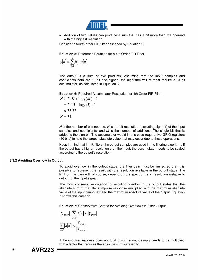
• Addition of two values can produce a sum that has 1 bit more than the operandwith the highest resolution.

2527B-AVR-07/08

[ ] [ ]∑ ⋅=4

j nxbny

34

32.33

1)5(log152

1)(log2

2

2

=

≈

++⋅=

Consider a fourth order FIR filter described by Equation 5.

Equation 5: Difference Equation for a 4th Order FIR Filter.

=0j

The output is a sum of five products. Assuming that the input samples andcoefficients both are 16-bit and signed, the algorithm will at most require a 34-bitaccumulator, as calculated in Equation 6.

Equation 6: Required Accumulator Resolution for 4th Order FIR Filter.

+⋅≥ +

N

M K N

N is the number of bits needed, K is the bit resolution (excluding sign bit) of the inputsamples and coefficients, and M is the number of additions. The single bit that isadded is the sign bit. The accumulator would in this case require five GPIO registers(40 bits) to hold the largest absolute value that may occur due to these operations.

Keep in mind that in IIR filters, the output samples are used in the filtering algorithm. If

the output has a higher resolution than the input, the accumulator needs to be scaledaccording to the output’s resolution.

3.3.2 Avoiding Overflow in Output

To avoid overflow in the output stage, the filter gain must be limited so that it ispossible to represent the result with the resolution available in the output stage. Thelimit on the gain will, of course, depend on the spectrum and resolution (relative tooutput) of the input signal.

The most conservative criterion for avoiding overflow in the output states that theabsolute sum of the filter’s impulse response multiplied with the maximum absolutevalue of the input cannot exceed the maximum absolute value of the output. Equation

7 shows this criterion.

Equation 7: Conservative Criteria for Avoiding Overflows in Filter Output.

[ ]

[ ]MAX

MAX

n

MAX

n

MAX

X

Y nh

Y nhX

≤

≤⋅

∑

∑∞

=

∞

=

0

0

If the impulse response does not fulfill this criterion, it simply needs to be multiplied

with a factor that reduces the absolute sum sufficiently.



AVR223

Keep in mind that for signed integers, the maximum value of the positive range is 1smaller than the absolute maximum value of the negative range. Assuming the inputis M-bit and the output is N-bit, Equation 8 shows the criterion for the worst-casescenario.

Equation 8: "Worst-Case" Conservative Criterion for Signed Integers.

7

2527B-AVR-07/08

[ ]∑ −

− −≤

1

1

2

12M

N

nh

Although fulfillment of this criterion guarantees that no overflow will ever occur, thedrawback is a substantial reduction of the filter gain. The characteristics of the inputsignal may be so that this criterion is overly pessimistic.

Another common criterion, which is better for narrowband signals (such as a sine),states that the absolute maximum gain of the filter multiplied with the absolute

maximum value of the input cannot exceed the absolute maximum value of theoutput. Equation 9 shows this criterion.

Equation 9: Criterion for Avoiding Overflow with Narrowband Signals.

MAX

MAX

H

MAX MAX H

X

Y H

Y H X

≤

≤⋅

)(max

)(max

)(

)(

ω

ω

ω

ω

This is the criterion used for the filter implementations in this application note: With

the same resolution in input and output, the filters should not exceed unity (0 dB)gain.

Note that the limit on the gain depends on the characteristics of the input signal, sosome experimentation may be necessary to find an optimal limit.

3.4 Scaling of Coefficients

Another important issue is the representation of the filter coefficients on Fixed Point(FP) architectures. FP representation does not necessarily mean that the values mustbe integers: As mentioned, fractional FP multiplication is also available. However, inthis application note only integer multiplications are used, and thus the focus is oninteger representations.

Naturally, to most accurately represent a number, one should use as many bits aspossible. For the purpose of using fractional filter coefficients in integermultiplications, this issue boils down to scaling all the coefficients by the largestcommon factor that does not cause any overflows in their representation. This scalingalso applies to the a0 coefficient, so a downscaling of the output is necessary to getthe correct value (especially for IIR filters). Division is not implemented in hardware,so the scaling factor should be on the form 2

ksince division and multiplication by

factors of 2 may easily be done with bitshifts. The principle of coefficient scaling andsubsequent downscaling of the result is shown in Equation 10.



8 AVR2232527B-AVR-07/08

[ ] [ ]

[ ] ( ) [ ] ( ) [ ] k inyajnxbny

jnxbinya

M

i

i

k N

j

j

k

N

j

j

k M

i

i

k

>>⎟⎟⎠

⎞⎜⎜⎝

⎛ −⋅⋅−+−⋅⋅=

−⋅=−⋅

∑∑

∑∑

==

==

10

00

22

22

Equation 10: Scaling of Filter Coefficients and Downscaling of Result.

Note that the sign bit must be preserved when downscaling. This is easily done withthe ASR instruction (arithmetic shift right).

As an example, consider the filter coefficients bj = {0.9001, -0.6500, 0.3000}. If 16-bitsigned integer representation is to be used, the scaled coefficients must have valuesin the range [-2

15…2

15-1] = [-32768…32767]. Naturally, the coefficient with the largest

absolute value will be the one limiting the maximum scaling factor. In this case, the

largest possible scaling factor without any overflow is 2

15

. Rounding of the scaledcoefficients results in the values {29494, -21299, 9830} and the approximate(downscaled) absolute rounding errors {1.5·10

-5, 6.1·10

-6, 1.2·10

-5}.

Optimization of the downscaling is possible if the factor k is above a multiple of 8. Ifthis is the case, the program may simply “ignore” bytes of the result. An example isillustrated in Figure 3-1, where a 32-bit result should be downscaled by 218. This isaccomplished by bit shifting the 16 Most Significant Bits (MSB) two times.

Figure 3-1: Optimized Downscaling (Grey Blocks are Unused Bits).

16-bit

6 bits 10 bits

8 bits8 bits

28 bits4 bits

x·218

32-bit

Filter input

6 bits 10 bits

Filter output

Accumulator

ACC >> 2

16-bit

3.4.1 Effect of Downscaling

One may wonder why one adds bits to avoid overflow in the sub-results, thenbasically “throws them away” to fit the result into a specified resolution. Theexplanation is that the bits are needed for precision during calculations, the filter hasunity gain, and the output should be interpreted as an integer.

For filters with unity gain, the coefficients will be fractional, i.e., less than one, andthus the multiplications will add bits that actually represent fractional values. Thesummations will, however, add bits that represent higher significance. But due to theunity gain of the filter, these bits will never be used in the result: The output of thefilter will not get an absolute value higher than that of the input, thus allowing theoutput to be represented with the same integer range as the input.



AVR223

9

2527B-AVR-07/08

The downscaling simply removes the fractional part of the result, leaving just theinteger part in the wanted resolution. Clearly, this also means that the precision isreduced. This is of consequence to IIR filters, since they have feedback. If the effectof this precision loss is a problem, it may be reduced in two ways:

• Maximize filter gain, so the output uses the entire, available range.

• Increase both the resolution of the output and the filter gain.

Of the two, only the latter can affect code size and throughput since a largeraccumulator may be required.

3.4.2 Reduced Resolution for Increased Throughput

To speed up the filtering algorithm, it may be desirable to reduce the resolution of thecoefficients and/or input samples so that the size of the accumulator can be reduced.A smaller accumulator means that the algorithm requires fewer operations permultiplication of filter coefficient and sample. However, two issues need to be takeninto consideration before doing this:

• Reduction of input sample resolution means that noise is introduced in the system,which is generally undesirable.

• Reduction of filter coefficient resolution means that the desired filter response maybecome harder to achieve.

For other ways to increase throughput, see “Optimization of Filter Implementations”on page 16.

4 Filter Implementations

The example filters in this application note were developed and compiled using theIAR EWAVR compiler version 5.03A.

The filter coefficients were calculated using software made for this purpose. There isa plethora of software that can do this, ranging from costly mathematical programssuch as Matlab™, to freely available Java applets on the web. A list of web sites thatdeal with the topic of calculating filter coefficients are provided in the literature listenclosed last in this application note. An alternative is to calculate the coefficients the“hard” way: By hand. Methods for calculating the filter coefficients (and investigatingstability of these filters) are described in [1] and [2].

Two filters are implemented; A fourth order High Pass (HP) FIR filter, and a secondorder Band Pass (BP) IIR filter. For both implementations, 10-bit signed inputsamples are used. The FIR filter uses 13-bit signed coefficients, while the IIR filteruses 12-bit signed coefficients. This is ensures that a maximum accumulator size of24 bits is needed.

The filters are implemented in assembly for efficiency reasons. The implementationsare made in such a way that the filter function can be called from C. Prior to callingthe filter functions, it is required that the filter nodes (memory of the delay elements)are initialized – otherwise the startup conditions of the filters are unknown. For bothfilters, a C code example that initializes and calls the filter function is provided.

All parameters required for filtering are passed at run time, so the filter function maybe reused to implement more than one filter without the need for additional codespace. This may be utilized for cascade coupling of filters: Often, multiple secondorder filters are used to form higher order filters by feeding the output of one filter intothe input of the next filter in the cascade. However, since the output from each filter in



10 AVR223

the cascade is downscaled before being fed into the next filter, the final output mightnot be as expected. This is because precision is lost in between filters. Naturally, theeffect of this becomes more pronounced with increased cascade lengths.

The implementations focus on fast execution of the filters, since a high throughput inthe filters is of great importance. See “Optimization of Filter” on page 16 forsuggestions on ways to reduce code size, increase throughput further, and reducememory usage.

4.1 Fourth Order FIR Filter

For the purpose of demonstrating the cascading technique, this filter is implementedby using two second order HP filters. Both filters were made with the windowingtechnique, described in [1], using a Hamming window. The filter parameters areshown in Table 4-1. Figure 4-1 shows the magnitude response of both filtersseparately, and in cascade.

Table 4-1: Second Order FIR Filter Parameters.

Filter Order Cutoff Coefficients (b0, b1, b2) Scaling

Scaled Coefficients

(b0, b1, b2)

No. 1 2 0.4 -0.0373, 0.9253, -0.0373 212

-153, 3790, -153

No. 2 2 0.6 -0.0540, 0.8920, -0.0540 212

-222, 3653, -222

Figure 4-1: Magnitude Response of FIR Filters.

The filter routines are implemented in assembly to make them efficient. However, thefilter parameters and the filter nodes need to be initialized prior to calling the filteringfunction. The initialization is done in C. A struct containing the filter coefficients andthe filter nodes are defined for each of the filters. The structs are defined as follows:

2527B-AVR-07/08



AVR223

11

2527B-AVR-07/08

struct FIR_filter{

int filterNodes [FILTER_ORDER]; //Filter nodes memory

//Filter coefficients memory

int filterCoefficients[FILTER_ORDER+1];

} filter04 = {0,0, B10, B11, B12}, //Init filter No. 1

filter06 = {0,0, B20, B21, B22}; //Init filter No. 2

The filterNodes array is used as a FIFO buffer, holding previous input samples.The filterCoefficients array is used for the feedforward coefficients of the filter.Once the filter is initialized the filter function can be called. The filter function isdefined as follows:

int FIR2(struct FIR_filter *myFilter, int newSample);

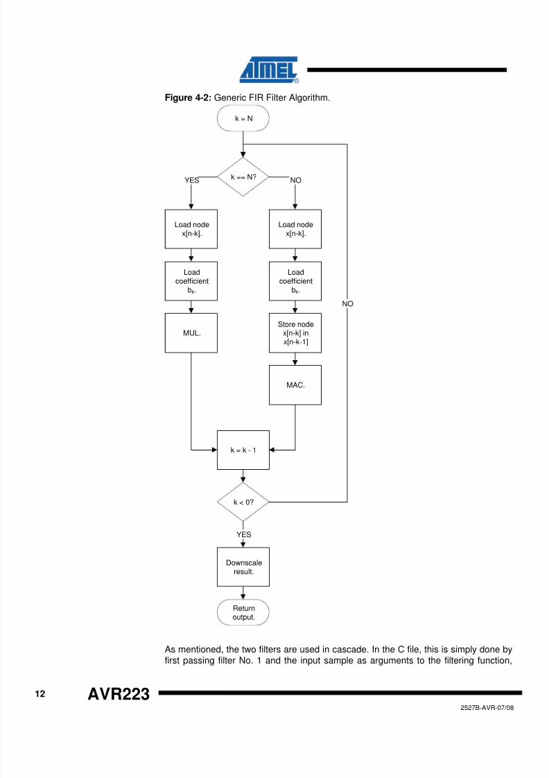
First, the function copies the pointer to the filter struct into the Z-register, since thismay be used for indirect addressing of data, i.e., for pointer operations. Then the coreof the algorithm is ready to be run. The samples (nodes) are loaded and multiplied(MUL) with the corresponding coefficients. The products are added in the 24-bit wideaccumulator. When all samples and coefficients are multiplied-and-accumulated(MAC), the result is downscaled and returned. This can be seen from the flow chart inFigure 4-2, which is a general description of the flow in a FIR filter algorithm.

Note that although the flow chart in Figure 4-2 shows the algorithm as if it wasimplemented using loops, the algorithm is actually implemented as straight-line code.The loop is used simply to improve readability.



12 AVR223

Figure 4-2: Generic FIR Filter Algorithm.

2527B-AVR-07/08

k == N?

Load nodex[n-k].

Load nodex[n-k].

Loadcoefficient

bk.

Loadcoefficient

bk.

MUL.Store node

x[n-k] inx[n-k-1]

MAC.

k = k - 1

k < 0?

Downscaleresult.

k = N

YES NO

YES

NO

Returnoutput.

As mentioned, the two filters are used in cascade. In the C file, this is simply done byfirst passing filter No. 1 and the input sample as arguments to the filtering function,



AVR223

13

2527B-AVR-07/08

then passing filter No. 2 and the output of the first filter as arguments to the samefunction.

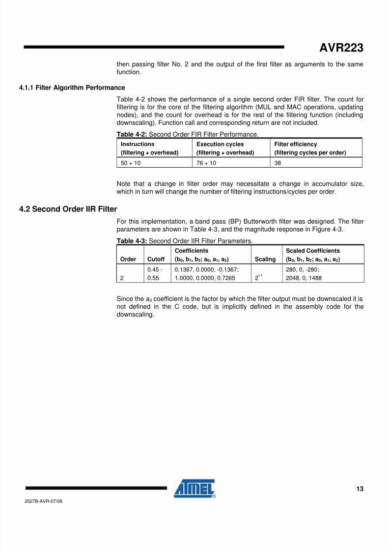
4.1.1 Filter Algorithm Performance

Table 4-2 shows the performance of a single second order FIR filter. The count forfiltering is for the core of the filtering algorithm (MUL and MAC operations, updatingnodes), and the count for overhead is for the rest of the filtering function (includingdownscaling). Function call and corresponding return are not included.

Table 4-2: Second Order FIR Filter Performance.

Instructions

(filtering + overhead)

Execution cycles


Filter efficiency

(filtering cycles per order)

50 + 10 76 + 10 38

Note that a change in filter order may necessitate a change in accumulator size,

which in turn will change the number of filtering instructions/cycles per order.

4.2 Second Order IIR Filter

For this implementation, a band pass (BP) Butterworth filter was designed. The filterparameters are shown in Table 4-3, and the magnitude response in Figure 4-3.

Table 4-3: Second Order IIR Filter Parameters.

Order Cutoff

Coefficients

(b0, b1, b2; a0, a1, a2) Scaling

Scaled Coefficients

(b0, b1, b2; a0, a1, a2)

2

0.45 -

0.55

0.1367, 0.0000, -0.1367;

1.0000, 0.0000, 0.7265 211

280, 0, -280;

2048, 0, 1488

Since the a0 coefficient is the factor by which the filter output must be downscaled it isnot defined in the C code, but is implicitly defined in the assembly code for thedownscaling.



Figure 4-3: Magnitude Response of Fourth Order IIR Filter.

A struct containing the filter coefficients and the filter nodes are defined for the filter.The filter should be initialized before the filter function is called. The struct is definedas follows:

struct IIR_filter{

int filterNodesX[FILTER_ORDER]; //filter nodes, stores x(n-k)

int filterNodesY[FILTER_ORDER]; //filter nodes, stores y(n-k)

//filter feedforward coefficients

int filterCoefficientsB[FILTER_ORDER+1];

//filter feedback coefficients

int filterCoefficientsA[FILTER_ORDER];

} filter04_06 = {0,0,0,0, B0, B1, B2, A1, A2}; //Init filter

The filterNodesX and filterNodesY arrays are used as FIFO buffers, holding

previous input and output samples respectively. The filterCoefficientsB and filterCoefficientsA arrays are used for the feed-forward and feedbackcoefficients of the filter respectively. Once the filter is initialized the filter function canbe called. The filter function is defined as follows:

int IIR2(struct IIR_filter *myFilter, int newSample);

The function first copies the pointer to the filter struct into the Z-register, since this canbe used for indirect addressing of data, i.e., for pointer operations. Then the core ofthe algorithm is ready to be run. The samples (data) are loaded and multiplied withthe matching coefficients. The products are added in the 24-bit wide accumulator.

14 AVR2232527B-AVR-07/08



AVR223

When all data and coefficients are Multiplied-and-Accumulated (MAC) and the filternode FIFO buffers are updated, the result is finally scaled down and returned. Notethat the result in the accumulator is downscaled before it is stored in the y[n-1] FIFObuffer element. A data flow chart is shown in Figure 4-4.

Figure 4-4: Generic IIR Filter Algorithm.

k == N?

Load nodex[n-k]. Load nodex[n-k].

Load

coefficientbk.

Load

coefficientbk.

MUL.Store node

x[n-k] in

x[n-k-1]

MAC.

k = k - 1

k < 0?

YES NO

YES

NO

k = N

k = N

Load nodey[n-k].

Load

coefficientak.

MAC.

k = k - 1

k < 1?

Downscaleresult.

Store nodey[n] iny[n-1].

Returnoutput.

YES

Store nodey[n-k] in

y[n-k-1].

NO

15

2527B-AVR-07/08



16 AVR2232527B-AVR-07/08

The flow chart in Figure 4-4 shows the algorithm as if it was implemented using loops,this is only to increase the readability of the flow chart. The algorithm is implementedusing straight-line code.

4.2.1 Filter Algorithm Performance

Table 4-4 shows the performance of the second order IIR filter. The count for filteringis for the core of the filtering algorithm (MUL and MAC operations, updating nodes),and the count for overhead is for the rest of the filtering function (includingdownscaling). Function call and corresponding return are not included.

Table 4-4: Fourth Order IIR Filter Performance.

Instructions


Execution Cycles


Filter Efficiency

(filtering cycles per order)

86 + 8 132 + 8 66

Note that a change in filter order may necessitate a change in accumulator size,which in turn will change the number of filtering instructions/cycles per order.

5 Optimization of Filter Implementations

The filters implemented in this application note were made efficient, but still easy toadapt to different filters. Because of this, they are sub-optimal. Below are suggestedways to optimize filters with regards to code size and/or throughput.

5.1 Improving Both Code Size and Throughput

One way to improve both code size and throughput is to ensure that only meaningful

calculations are performed. The assembly code for the filters implemented in thisapplication note is made so that it will work with any set of filter coefficients. However,the second order IIR example filter has two zero-coefficients. Multiplication andsubsequent accumulation with zero-coefficients may, of course, be omitted as it willnot contribute to the output. This way, the code size is reduced and throughputincreased.

5.2 Reducing Code Size

A reduction of code size may be achieved by implementing the MAC operation as afunction call, instead of as a macro. However, this will impact the throughput sinceeach function call and corresponding return will consume additional cycles.

Another way to reduce the code size is to implement high-order filters as cascades oflower order filters, as demonstrated in the fourth order FIR example filter. Though, asmentioned earlier, this will reduce the precision of the filter due to the downscaling inbetween each filter in the cascade. Also, optimizing by omitting MAC operations withzero-coefficients may not be possible in such implementations.

5.3 Reducing Memory Usage

The filter coefficients have in both example implementations simply been put inSRAM. A simple way to reduce memory usage is to put the coefficients in FLASH andfetch when needed. This will potentially almost halve the memory usage for the filterparameters, since there are almost as many coefficients as there are filter nodes

(previous input/output samples).



AVR223

17

2527B-AVR-07/08

6 References

[1] “Discrete-Time signal processing”, A. V. Oppenheimer & R. W. Schafer. Prentice-

Hall International Inc. 1989. ISBN 0-13-216771-9[2] “Introduction to Signal Processing”, S. J. Orfanidis, Prentice Hall International Inc.,1996. ISBN 0-13-240334-X

[3] FIR filter design, http://www.iowegian.com/scopefir.htm

[4] FIR filter design,http://www.dsptutor.freeuk.com/FIRFilterDesign/FIRFiltDes102.html

[5] FIR filter design,http://www.dsptutor.freeuk.com/KaiserFilterDesign/KaiserFilterDesign.html

[6] IIR filter design, http://www.apogeeddx.com/BQD_Appnote.PDF

[7] IIR filter design, http://moshier.ne.mediaone.net/ellfdoc.html

[8] FIR and IIR filter design, http://www-users.cs.york.ac.uk/~fisher/mkfilter/

[9] FIR and IIR filter design, http://www.nauticom.net/www/jdtaft/papers.htm



Disclaimer

Headquarters International

Atmel Corporation 2325 Orchard Parkway San Jose, CA 95131 USA Tel: 1(408) 441-0311 Fax: 1(408) 487-2600

Atmel Asia Room 1219 Chinachem Golden Plaza 77 Mody Road Tsimshatsui East Kowloon Hong Kong Tel: (852) 2721-9778 Fax: (852) 2722-1369

Product Contact

Atmel Europe Le Krebs 8, Rue Jean-Pierre Timbaud BP 309 78054 Saint-Quentin-en-Yvelines Cedex France Tel: (33) 1-30-60-70-00 Fax: (33) 1-30-60-71-11

Atmel Japan 9F, Tonetsu Shinkawa Bldg. 1-24-8 Shinkawa Chuo-ku, Tokyo 104-0033 Japan Tel: (81) 3-3523-3551 Fax: (81) 3-3523-7581

Web Site www.atmel.com

Technical Support [email protected]

Sales Contact www.atmel.com/contacts

Literature Request

www.atmel.com/literature

Disclaimer: The information in this document is provided in connection with Atmel products. No license, express or implied, by estoppel or otherwise, to anyintellectual property right is granted by this document or in connection with the sale of Atmel products. EXCEPT AS SET FORTH IN ATMEL’S TERMS ANDCONDITIONS OF SALE LOCATED ON ATMEL’S WEB SITE, ATMEL ASSUMES NO LIABILITY WHATSOEVER AND DISCLAIMS ANY EXPRESS, IMPLIEDOR STATUTORY WARRANTY RELATING TO ITS PRODUCTS INCLUDING, BUT NOT LIMITED TO, THE IMPLIED WARRANTY OF MERCHANTABILITY,FITNESS FOR A PARTICULAR PURPOSE, OR NON-INFRINGEMENT. IN NO EVENT SHALL ATMEL BE LIABLE FOR ANY DIRECT, INDIRECT,CONSEQUENTIAL, PUNITIVE, SPECIAL OR INCIDENTAL DAMAGES (INCLUDING, WITHOUT LIMITATION, DAMAGES FOR LOSS OF PROFITS,BUSINESS INTERRUPTION, OR LOSS OF INFORMATION) ARISING OUT OF THE USE OR INABILITY TO USE THIS DOCUMENT, EVEN IF ATMEL HASBEEN ADVISED OF THE POSSIBILITY OF SUCH DAMAGES. Atmel makes no representations or warranties with respect to the accuracy or completeness of thecontents of this document and reserves the right to make changes to specifications and product descriptions at any time without notice. Atmel does not make anycommitment to update the information contained herein. Unless specifically provided otherwise, Atmel products are not suitable for, and shall not be used in,automotive applications. Atmel’s products are not intended, authorized, or warranted for use as components in applications intended to support or sustain life.

© 2008 Atmel Corporation. All rights reserved. Atmel®, logo and combinations thereof, AVR® and others, are the registered trademarks or

trademarks of Atmel Corporation or its subsidiaries. Other terms and product names may be trademarks of others.

avr223 digital filters with avr

Documents