1

Avisoft-SASLab Pro version 5.2

Sound Analysis and Synthesis Laboratory for Microsoft Windows XP / Vista / 7 / 8 / 8.1 / 10 Avisoft Bioacoustics e.K. Schönfließer Str. 83 16548 Glienicke/Nordbahn GERMANY www.avisoft.com support avisoft.com

2

LICENSE AGREEMENT This is a legal agreement between Avisoft Bioacoustics and the buyer. By operating this software, the buyer accepts the terms of this agreement. 1. Avisoft Bioacoustics (the „Vendor“) grants to the Buyer a non-exclusive license to operate the provided software (the „Software“) on ONE computer at a time. 2. The Software is the exclusive property of the Vendor. The Software and all documentation are copyright Avisoft Bioacoustics, all rights reserved. 3. The Software is warranted to perform substantially in accordance with the operating manual for a period of 24 months from the date of shipment. 4. EXCEPT AS SET FORTH IN THE EXPRESS WARRANTY ABOVE, THE SOFTWARE IS PROVIDED WITH NO OTHER WARRANTIES, EXPRESS OR IMPLIED. THE VENDOR EXCLUDES ALL IMPLIED WARRANTIES, INCLUDING, BUT NOT LIMITED TO, IMPLIED WARRANTIES OF MERCHANTIBILITY AND FITNESS FOR A PARTICULAR PURPOSE. 5. The Vendor’s entire liability and the Buyer’s exclusive remedy shall be, at the Vendor’s SOLE DISCRETION, either (1) return of the Software and refund of purchase price or (2) repair or replacement of the Software. 6. THE VENDOR WILL NOT BE LIABLE FOR ANY SPECIAL, INDIRECT, OR CONSEQUENTIAL DAMAGES HEREUNDER, INCLUDING, BUT NOT LIMITED TO, LOSS OF PROFITS, LOSS OF USE, OR LOSS OF DATA OR INFORMATION OF ANY KIND, ARISING OUT OF THE USE OF OR INABILITY TO USE THE SOFTWARE IN NO EVENT SHALL THE VENDOR BE LIABLE FOR ANY AMOUNT IN EXCESS OF THE PURCHASE PRICE. 7. This agreement is the complete and exclusive agreement between the Vendor and the Buyer concerning the Software.

3

CONTENTS

INTRODUCTION ................................................................... 18

HARD- & SOFTWARE REQUIREMENTS ............................ 18

INSTALLATION PROCEDURE ............................................. 19

PROGRAM DESCRIPTION ................................................... 20

Getting started ...................................................................................................... 20

THE MAIN WINDOW ............................................................. 22

File .......................................................................................................................... 22

Open ............................................................................................................. 22 Browse… .......................................................................................................... 22 File Open Settings… ......................................................................................... 23 Close ................................................................................................................. 25 Save ................................................................................................................... 25

Save As... ................................................................................................ 26 Rename ............................................................................................................. 26 Rename by text module / Define text module > ................................................ 26

Record .................................................................................................. 27

Real Time Spectrogram .......................................................................... 27

4

Sound card settings ................................................................................. 28

Playback ............................................................................................. 29 Playback settings… .......................................................................................... 29 Heterodyned playback mode… ........................................................................ 30 Play through RECORDER USGH / UltraSoundGate Player ........................... 30 Route UltraSoundGate DIO track (LTC) to the right playback channel .......... 31 Configuration > ................................................................................................ 31 Open... .............................................................................................................. 31 Save .................................................................................................................. 31 Save As... .......................................................................................................... 31 Reset ................................................................................................................. 31 Save mode on exit > ......................................................................................... 32 Save current configuration automatically ......................................................... 32 Prompt .............................................................................................................. 32 Open mode on start > ....................................................................................... 32 Open last configuration automatically .............................................................. 32 Launch Open dialog ......................................................................................... 32 DDE Command Interface ................................................................................. 33 Specials > ......................................................................................................... 33 Previous file...................................................................................................... 33 Next file ............................................................................................................ 33 Previous/Next file command settings… ........................................................... 34 Auto Browse ..................................................................................................... 34 Delete File ........................................................................................................ 34 Re-assembling settings… ................................................................................. 34 Import-Format .................................................................................................. 35 File properties ................................................................................................... 36 Add channel(s) from file .................................................................................. 36 Add silent channel ............................................................................................ 37 Remove channels .............................................................................................. 37 Add neighbour channels automatically ............................................................ 37 Swap channels .................................................................................................. 37 Insert .wav file .................................................................................................. 37 Append .wav file .............................................................................................. 37 Join .wav files ................................................................................................... 37 Join .wav files from a playlist........................................................................... 37 UltraDoundGate DIO ....................................................................................... 38 Shred into numbered files... .............................................................................. 39 Envelope ........................................................................................................... 39 Save Envelope Curve ....................................................................................... 39 Copy Envelope Curve ...................................................................................... 39 Envelope Curve Export Parameters .................................................................. 39

5

Launch separate Curve Window ....................................................................... 40 Real Time Spectrum .......................................................................................... 40 Don’t work on copies of opened .wav files ....................................................... 40 Georeference .wav files ..................................................................................... 40 Edit title ............................................................................................................. 43 New Instance ..................................................................................................... 43

Marking time sections .......................................................................................... 43

Analyze .................................................................................................................. 44

Create spectrogram .................................................................................. 44

Spectrogram-Parameters ......................................................................... 44

Spectrogram Overview ............................................................................ 49

Overview Parameters .............................................................................. 50 Apply spectrogram window parameters ............................................................ 51 Normalize Envelope Curve ............................................................................... 51 Show Y axis grid ............................................................................................... 51 Frequency cursor ............................................................................................... 51 Step waveform display mode ............................................................................ 51 Fast Envelope Curve display ............................................................................. 51 Time axis format ............................................................................................... 51 One-dimensional transformations ..................................................................... 53 Time signal ........................................................................................................ 53 Amplitude spectrum .......................................................................................... 53 Power spectrum (logarithmic) ........................................................................... 54 Power spectrum (averaged) ............................................................................... 54 Power spectrum (spectrum level units) ............................................................. 54 Power spectrum (level units, averaged) ............................................................ 54 Octave Analysis ................................................................................................ 55 Third-Octave Analysis ...................................................................................... 55 Autocorrelation ................................................................................................. 55 Cepstrum ........................................................................................................... 55 Cross-correlation (stereo) .................................................................................. 55 Cross-correlation (2 files) ................................................................................. 56 Transfer function (2 stereo channels) ................................................................ 56 Frequency response, sine sweep mono.............................................................. 56 Frequency response, sine sweep stereo ............................................................. 57 Histogram .......................................................................................................... 57 XY Plot ............................................................................................................. 57 XYZ Plot ........................................................................................................... 57

6

Impulse Density Histogram .............................................................................. 57 Impulse Rate ..................................................................................................... 58 Lorenz plot ....................................................................................................... 58 Envelope (analytic signal) ................................................................................ 59 Instantaneous frequency ................................................................................... 59 Zero-crossing analysis ...................................................................................... 59 Root mean square (linear) / (logarithmic) ........................................................ 59 Envelope ........................................................................................................... 60 Gate function .................................................................................................... 60 Gate function (signal/silence duration)............................................................. 60 Gate function (interpulse interval) .................................................................... 60 Pulse Train Analysis ......................................................................................... 61 Settings… ......................................................................................................... 62 Specials > ......................................................................................................... 72 Copy energy of marked section ........................................................................ 72 Copy RMS of marked section .......................................................................... 72 Copy peak-to-peak of marked section .............................................................. 72 Time-delay-of-arrival (TDOA) measurements ................................................. 72 Detect waveform events and create section labels ........................................... 73 Detect and classify waveform events ............................................................... 73 Scan for template spectrogram patterns............................................................ 74

Edit ........................................................................................................................ 76

Undo ....................................................................................................... 76

Redo ....................................................................................................... 76

Copy ........................................................................................................ 76

Paste ........................................................................................................ 76

Cut .......................................................................................................... 76 Trim .................................................................................................................. 76 Change Volume ................................................................................................ 76 Delete ............................................................................................................... 78 Delete with taper .............................................................................................. 78 Insert silence ..................................................................................................... 78 Insert silent margins ......................................................................................... 78 Mix ................................................................................................................... 78 Reverse ............................................................................................................. 78

Info about Clipboard .............................................................................. 78 Compress > ....................................................................................................... 80

7

Remove silent sections ...................................................................................... 80 Settings .............................................................................................................. 80 Remove gaps between section labels ................................................................ 80 Remove gaps between (section) labels and keep labels .................................... 81 Expanded view (restored time structure) ........................................................... 81 Save segments into numbered .wav files ........................................................... 81 Synthesizer > ..................................................................................................... 81 Synthesizer (dialog-based)... ............................................................................. 81

Synthesizer (graphically)... ..................................................................... 81 Insert white noise… .......................................................................................... 82 Insert pink noise… ............................................................................................ 82 Insert time code / pulse train / single pulse… ................................................... 82 Filter > ............................................................................................................... 82 IIR Time Domain Filter .................................................................................... 82

FIR Time Domain Filter ......................................................................... 84 Frequency Domain Transformations (FFT) ...................................................... 87 Noise Reduction ................................................................................................ 89 Format > ............................................................................................................ 90 Stereo->Mono ................................................................................................... 90 8<-->16Bit Conversion ..................................................................................... 90 Change Fileheader Sampling Frequency / Time Expansion ............................. 90 Sampling frequency conversion... ..................................................................... 90 Restore the original time scale of a time-expanded recording .......................... 91 Time/Pitch Conversion… .................................................................................. 91

Tools ....................................................................................................................... 93

Zoom ...................................................................................................... 93

Unzoom .................................................................................................. 93 Zoom Previous .................................................................................................. 93 ZoomIn .............................................................................................................. 93 ZoomOut ........................................................................................................... 93 Remove Marker ................................................................................................. 93 Set Marker Duration .......................................................................................... 93 Copy Measurement values t1, t2 ....................................................................... 94 Cursor linkage between Instances… ................................................................. 94 Labels > ............................................................................................................. 94 Insert label ......................................................................................................... 94 Insert section label............................................................................................. 94 Insert section label from marker ........................................................................ 94 Create section labels from waveform events ..................................................... 94

8

Create labels from UltraSoundGate DI ............................................................ 96 Georeference labels / .wav files ........................................................................ 97 Delete all labels ................................................................................................ 98 Filter labels ....................................................................................................... 99 (Re-)Number labels .......................................................................................... 99 Label settings... ................................................................................................. 99 Import section labels from .txt file… ............................................................... 99 Import time-frequency labels from .txt file… .................................................. 99 Export labels into .txt file… ........................................................................... 100 Label statistics… ............................................................................................ 100 Export label data ............................................................................................. 100 Save labeled sections into numbered .wav files ............................................. 101 Save labeled sections into a single .wav file…............................................... 101 Save labeled sections of same class into single .wav files… .......................... 101 Classify labeled sections ................................................................................ 101 Detect and Classify waveform events ............................................................ 106 Classify Element Sequences ........................................................................... 106 Section label grid... ......................................................................................... 108 DDE parameters / Log-file... .......................................................................... 108 Touch Screen Optimizations .......................................................................... 108 Calibration ...................................................................................................... 110 Batch processing ............................................................................................ 114 Real-time processing ...................................................................................... 121

Metadata ............................................................................................................. 123 dXML database records > .............................................................................. 123 mXML measurements > ................................................................................. 125 View XML RIFF chunks > ............................................................................ 126 Select XML viewer... ..................................................................................... 126 bext (BWF) Metadata... > ............................................................................. 127 Edit ................................................................................................................. 127 Batch Edit ....................................................................................................... 127 Create Metadatabase... .................................................................................... 127 On new sound file > ....................................................................................... 134 Spectrogram ................................................................................................... 134 One-dimensional transformation .................................................................... 134 Pulse Train Analysis ....................................................................................... 134 Remove silent sections ................................................................................... 134 On program start > ......................................................................................... 134 Real-time spectrograph ................................................................................... 134 Graphic synthesizer ........................................................................................ 134 Launch Real-time spectrum display ............................................................... 134 Launch Real-time processing tool .................................................................. 134 Open last sound file ........................................................................................ 134

9

Keyboard Shortcuts and Popup Menu ............................................................. 134

THE SPECTROGRAM WINDOW ........................................ 135

File ........................................................................................................................ 135

Print Spectrogram ................................................................................. 135

Copy Spectrogram ................................................................................. 135

Save Spectrogram Image ....................................................................... 135 Copy entire Spectrogram Image ...................................................................... 135 Save entire Spectrogram Image ....................................................................... 135

Export-Parameters ................................................................................. 136 Data Export > .................................................................................................. 139 Copy measured value ...................................................................................... 139 Copy t1, t2 ....................................................................................................... 139 Copy energy of marked section ....................................................................... 139 DDE Parameters / Log File ............................................................................. 139 Copy ASCII Spectrum .................................................................................... 142 Copy ASCII Spectrogram ............................................................................... 142 Save ASCII/Binary Spectrogram .................................................................... 142 Copy ASCII-Frequency versus time ............................................................... 142 Copy Envelope into curve-window ................................................................. 142 Copy Spectrum into curve-window ................................................................. 142 Mean Spectrum of entire spectrogram ............................................................ 143 Max spectrum of entire element ...................................................................... 143 Copy Spectrogram into 3D curve-window ...................................................... 143 Power Spectrum .............................................................................................. 143

Display ................................................................................................................. 143

Display-Parameters... ........................................................................... 143 Grid ................................................................................................................. 143 Cut-Off Frequency .......................................................................................... 143

Additional Spectrogram Information .................................................... 144 Show the Spectrogram parameters of this spectrogram .................................. 145 Level Display Mode ........................................................................................ 146 Absolute Time Scaling .................................................................................... 146 Limit measurement decimal places to spectrogram resolution ....................... 146 Create Color Table .......................................................................................... 146

10

Hide buttons and numeric display area ........................................................... 147 Hide main window ......................................................................................... 147

Tools .................................................................................................................... 148

Playback .......................................................................................... 148 Playback settings… ........................................................................................ 148 Heterodyned playback mode… ...................................................................... 148 Enlarge Image ................................................................................................ 148 Reduce Image ................................................................................................. 148 Zoom out time axis ......................................................................................... 148 Scroll > ........................................................................................................... 149 Left, right, begin, end ..................................................................................... 149 Auto Scroll ..................................................................................................... 149 Image Filter: Average, Median ....................................................................... 149 Scan frequency contour and amplitude envelope ........................................... 149 Remove erased spectrogram sections from waveform ................................... 153 Cursors> ......................................................................................................... 154

How to use the measurement cursors ............................................................... 154 Marker mode .................................................................................................. 154

Cursor modes ................................ 155 Insert bound frequency cursor ........................................................................ 156 Insert frequency cursor ................................................................................... 156 Insert harmonic frequency cursor ................................................................... 156 Remove Marker .............................................................................................. 156 Remove Cursors ............................................................................................. 156 Erase marked section ...................................................................................... 156 (Move reticule cursor by one pixel) / left, right, up, down ............................. 156 Copy cursor value ........................................................................................... 156 Copy the marker to the main window ............................................................ 157 Cursor linkage between Instances .................................................................. 157 Display amplitude at reticule cursor cross ...................................................... 157 Magic reticule cursor ...................................................................................... 158 Labels > .......................................................................................................... 161

Labeling .............................................................................................................. 161 Insert label ...................................................................................................... 162 Insert section label .......................................................................................... 162 Insert section label from marker ..................................................................... 162 Section label grid... ......................................................................................... 162 Label settings... ............................................................................................... 162 Label statistics… ............................................................................................ 164

11

Export label data… ......................................................................................... 165

Automatic parameter measurements > ............................................................. 165

Classification ....................................................................................................... 184

Classification Settings ......................................................................................... 185 add class .......................................................................................................... 185 rename ............................................................................................................. 185 delete ............................................................................................................... 185 Location .......................................................................................................... 185 Copy settings ................................................................................................... 186 Reset ................................................................................................................ 186

Configuring the classification option ................................................................ 187

Automatic Parameter Measurements Statistics ............................................... 188 Numeric display .............................................................................................. 188 Minimum, Maximum, Mean, Median, Standard deviation ............................. 188 Relative on time (for duration only) ................................................................ 188 The relative on time corresponds to the sum of the element durations divided by

the total duration of the spectrogram (the option “Compute parameters from

entire spectrogram must be activated”). .......................................................... 188 Histogram of one parameter ............................................................................ 188 Update ............................................................................................................. 189 Copy parameter measurement values .............................................................. 189 Copy parameter measurement values for entire file ........................................ 189 Copy parameter measurement values in transposed order .............................. 189 Copy parameter measurement headings .......................................................... 189 Save detected elements into numbered .wav files ........................................... 189 Remove gaps between detected elements ....................................................... 190 Copy detected elements into section labels ..................................................... 190 Copy peak frequencies into labels ................................................................... 191 Keyboard Shortcuts and Popup Menu ............................................................. 191

WavFile ................................................................................................................ 191 Open... ............................................................................................................. 191 Browse ............................................................................................................ 192 Rename ........................................................................................................... 192 Rename by text module ................................................................................... 192 Import Format ................................................................................................. 192 Spectrogram parameters... ............................................................................... 192 Copy : .............................................................................................................. 192 Save As… ....................................................................................................... 192

12

New instance .................................................................................................. 192 Save configuration .......................................................................................... 192

Automatic Parameter Measurements display window ................................... 192 Setup ............................................................................................................... 193 Classification settings... .................................................................................. 193 Statistics settings.... ........................................................................................ 193 Compute parameters from entire spectrogram ............................................... 194 Export ............................................................................................................. 194 Copy parameter measurement values ............................................................. 194 Copy parameter measurement values for entire file ....................................... 194 Copy parameter measurement values in transposed order.............................. 194 Copy parameter measurement headings ......................................................... 194 Copy the time stamp of the selected element ................................................. 194 Copy class sequence ....................................................................................... 194 Copy class frequency ...................................................................................... 194 Save detected elements into numbered .wav files... ....................................... 195 Remove gaps between detected elements from sound file... .......................... 195 Copy detected elements into section labels .................................................... 195 DDE Parameters / Log-File. ........................................................................... 195 View ............................................................................................................... 195

Automatic Response ........................................................................................... 195 Methods of measurement value export ........................................................... 199

Spectrogram output ........................................................................................... 200

THE REAL-TIME SPECTRUM DISPLAY ........................... 201

THE CURVE WINDOW ....................................................... 201

File ....................................................................................................................... 202

Print ..................................................................................................... 202

Save ..................................................................................................... 202

Copy ..................................................................................................... 202

Export Parameters ................................................................................ 202 Data export > .................................................................................................. 204 Save ASCII file .............................................................................................. 204

13

Copy ASCII file ...................................................................................... 204 Add x axis increments ..................................................................................... 204 Save as .WAV file… ....................................................................................... 204 Copy WAV file ............................................................................................... 204 Save as .ft file… .............................................................................................. 204 Save as .flf file… ............................................................................................ 205 Copy cursor values .......................................................................................... 205 DDE Parameters / Log File ............................................................................. 205

Start real-time spectrum ........................................................................ 205

Stop real-time spectrum ........................................................................ 205 Real-time spectrum setup ................................................................................ 205 Sound card settings ......................................................................................... 205 Display ............................................................................................................ 206

Zoom ..................................................................................................... 206

Unzoom ................................................................................................. 206 Unzoom with zero ........................................................................................... 206

Zoom previous ..................................................................................... 206 Display range .................................................................................................. 206 Grid ................................................................................................................. 206 Steps ................................................................................................................ 207 3D Options... ................................................................................................... 207 Spectral Characteristics ................................................................................... 208 Pulse Train Analysis... .................................................................................... 210

Tools ..................................................................................................................... 211 Insert bound cursor .......................................................................................... 211 Insert free horizontal cursor ............................................................................ 211 Remove cursor ................................................................................................ 211 Harmonic cursor .............................................................................................. 211 Cursor linkage between Instances… ............................................................... 211 Insert label ....................................................................................................... 211 Insert section label........................................................................................... 211 Label settings... ............................................................................................... 211 Generate section labels .................................................................................... 211 Keyboard Shortcuts and Popup Menu ............................................................. 212

Edit ....................................................................................................................... 212 Smooth ............................................................................................................ 212 Power spectrum ............................................................................................... 212 Normalize to maximum ................................................................................... 212

14

The Real Time Spectrograph Window ................................................. 213 File.................................................................................................................. 214 Record ............................................................................................................ 214 Automatic Recording... .................................................................................. 215 Automatic Response Setup.. ........................................................................... 216

Reset overflow flag ................................................................................. 216 Freeze display (toggle) ................................................................................... 216 Trigger ............................................................................................................ 216 Threshold ........................................................................................................ 216 Frequency domain .......................................................................................... 216 Hold time ........................................................................................................ 216 Minimum duration .......................................................................................... 216 File name ........................................................................................................ 217 Reset ............................................................................................................... 217 Save all events into a single file ..................................................................... 217 Buffer Size... ................................................................................................... 217 Envelope ......................................................................................................... 218 Scroll-Mode .................................................................................................... 218 Sound Card Settings... .................................................................................... 218 Export-Parameters... ....................................................................................... 218 Keyboard Shortcuts and Popup Menu ............................................................ 218

SYNTHESIZER (DIALOG-BASED) .................................... 219

GRAPHIC SYNTHESIZER .................................................. 223

File ....................................................................................................................... 224 New ................................................................................................................ 224

Open... .................................................................................................. 224

Save ..................................................................................................... 224 Save as... ......................................................................................................... 225

Setup .................................................................................................. 225 Sine generator ................................................................................................. 225 Noise generator .............................................................................................. 226 Pulse train generator ....................................................................................... 227

Play ................................................................................................... 227

15

Insert .................................................................................................... 227 Insert into clipboard ........................................................................................ 227 Save into WAV file ......................................................................................... 228 Sampling rate settings… ................................................................................. 228 Open last arrangement on start ........................................................................ 228

Tools ..................................................................................................................... 228

Zoom .................................................................................................... 228

Unzoom ............................................................................................... 228 Unzoom with zero ........................................................................................... 228 View ................................................................................................................ 228 Grid ................................................................................................................. 228

Next element ......................................................................................... 228

Next point .............................................................................................. 228

Previous point ........................................................................................ 229

Previous element ................................................................................... 229

Delete point ........................................................................................... 229

Delete element ....................................................................................... 229

Lock time-axis ....................................................................................... 229

Lock Y-axis ........................................................................................... 229 Scan harmonics from spectrogram based on fundamental .............................. 229 Scaling ............................................................................................................. 230 Copy contour… ............................................................................................... 231

Edit ....................................................................................................................... 231 Copy ................................................................................................................ 231 Paste ................................................................................................................ 231 Cut ................................................................................................................... 231 Delete .............................................................................................................. 231 Append ............................................................................................................ 231 Remove marker ............................................................................................... 231 Disable marker ................................................................................................ 232

16

View ..................................................................................................................... 232 Display Spectrogram ...................................................................................... 232 Display Instantaneous frequency / Zero crossing analysis ............................. 232 Fundamental Frequency, Overall Amplitude, Rel. amplitude, ... ................... 232 Example of AM .............................................................................................. 233 Example of FM ............................................................................................... 233

GUIDELINES FOR MAKING CORRECT SPECTROGRAMS ............................................................................................ 234

Over-modulation ................................................................................................ 234

Aliasing ............................................................................................................... 234

THE AVISOFT-CORRELATOR .......................................... 235

How to use the Avisoft-CORRELATOR ......................................................... 235 Select the files to be compared ....................................................................... 235 Start the correlation process / Defining the correlation parameters ................ 236 Exporting the correlation matrix .................................................................... 237 Averaging of aligned spectrograms ................................................................ 237

The correlation algorithm ................................................................................. 239

Discussion of the correlation method ............................................................... 239

TUTORIAL .......................................................................... 241

Measuring sound parameters from the spectrogram manually ..................... 243 Labels ............................................................................................................. 246

Measuring sound parameters from the spectrogram automatically ............. 248 automatic (single threshold) ........................................................................... 249 automatic (two thresholds) ............................................................................. 252 automatic (three thresholds) ........................................................................... 254 interactively (section labels) ........................................................................... 256 automatic (whistle tracking) ........................................................................... 257

Basic Analysis of rat or mouse USV's .............................................................. 259

17

FURTHER READING .......................................................... 263

INDEX .................................................................................. 264

18

Introduction

The Avisoft-SASLab Pro software is a powerful spectrograph, synthesizer and

versatile signal analyzer for evaluating audio signals.

The signals sampled by a sound card are displayed as an envelope curve inside the

main window of the application. Optionally, there can be displayed an overview

spectrogram. The time data can be edited by different functions. After marking a

signal section, a spectrogram can be generated using the current spectrogram

parameter. This spectrogram is displayed in an extra window. Here several display

parameters (colors, threshold for black & white display, gradation) of the

spectrogram can be changed. The spectrogram can be exported into the Windows-

clipboard according to the previous defined export parameters. The spectrogram

can also be saved as BMP-or TIFF- graphics files. These exported spectrograms

can be read by different Windows-applications (Write, WinWord, Paintbrush,

PageMaker...). There they can be supplied with text information and can be

printed. For quantitative analysis the spectrogram can be measured by a set of

different cursors. The real time display makes it easy to check long sound

sequences.

The following introduction into the analysis of acoustic signals is addressed to

beginners, who want to become familiar with the foundations. The very special

mathematical details are suppressed for better understanding. Those, who want to

learn more about these details, should study the specialized literature about

telecommunications and digital signal processing.

Hard- & Software Requirements

To run the software, a Windows PC with at least 32 MB of RAM and about 10 MB

of free hard-disk space is required. For recording audio signals, a sound card

compatible to Windows should be installed. See the user's guide of the sound card

for installation instructions.

19

Installation procedure

To install the software, run the installation program either from the supplied USB

flash drive (subfolder SASLab Pro / setup.exe) or the Avisoft Bioacoustics

website (www.avisoft.com/downloads.htm or www.avisoft.com/SASLab Pro.exe).

The supplied Hardlock/HL key, which is required to run the software, should not

be connected to the computer before the software installation has finished.

A special Hardlock device driver (HaspUserSetup.exe) must be installed to enable

the Hardlock recognition. Usually, this driver is installed automatically when the

installation is started from the Avisoft Bioacoustics software installation media. A

separate Hardlock driver installation program can be found on the installation CD

or USB flash drive or at www.avisoft.com.

Free software updates that provide bug fixes and improved functionality are

available from www.avisoft.com.

20

Program description

The software is divided into three different windows. After starting the program

the main window appears. Here you can record audio data or load audio files,

which are displayed immediately as an envelope curve and optionally as an

overview spectrogram. Subsections of the whole file can be displayed

spectrographically in a separate spectrogram window. The real time spectrograph

window allows displaying of spectrograms in real-time.

Getting started

The following topics describe the spectrogram generation procedure.

Sound card adjustment : Selection of sampling frequency (see page 28)

Adjusting the recording level through the software supplied with the sound card

(menu option ”File”/”Recording Level Control...”).

Data acquisition: Start recording "File/Record" (see page 27), Stop

recording with . Alternatively the Real-Time-Spectrograph (Menu

"File/Real Time Spectrogram" ) can be used for pre-trigger data acquisition

(see page 213).

Select the section to be analyzed spectrographically by clicking on the desired

start point and dragging to the end point inside the envelope curve display. The

current selection can be verified by playing that section through the sound card

.

Adjusting the spectrogram parameter in the menu "Analyze/Spectrogram

parameters..." (see page 44).

Generate spectrogram (see page 44).

Select display-parameter inside the spectrogram window Display/ Display-

Parameter...) (see page 143).

In very long spectrograms the visible section can be selected using the

horizontal scroll bar at the bottom of the window. Please note, that the window

size can be changed by dragging the left and right window margins.

21

Adjusting the export-parameters for printing the spectrogram (menu

File/Export-Parameters...) (see page 136).

Print spectrogram directly using the menu "File/Print Spectrogram"

or:

Copy the spectrogram into the clipboard (menu File/Copy Spectrogram) .

Insert the spectrogram into a word processor or graphic editor application.

There you can input a documentation text before printing.

22

The main window

The main window supplies all functions necessary for recording, playing, editing

and displaying of time data (audible sound signals). The spectrogram generation is

parameterized and started here.

File

Open

The File/Open dialog allows to load previously saved sound files. It is also

possible to open sound files in other formats than WAV:

Avisoft-DOS (*.DAT) File format of the old DOS-based Avisoft-

SONAGRAPH.

NeXT/SUN (*.AU; *.SND) Standard sound file format on UNIX workstations.

Apple AIFF (*.AIF; *.SND) Standard sound file format on Apple-Macintosh.

User-defined (*.*) Other sound file formats which have been previously

defined in the menu "File/Import-Format...".

Alternatively sound files can be loaded by Drag&Drop technique. You have first to

start the Windows file manager. Then click at the desired file and drag the mouse

cursor to the Avisoft-SASLab window while the left mouse bottom is pressed.

Releasing the mouse bottom above Avisoft-SASLab will load this file.

Browse… This modeless dialog box allows quick navigation through sound files. All files

located in the specified Folder will be listed including date and titles read from the

23

.wav file chunks. The “…” button may be used to choose a file from a different

folder. A file can be opened by selecting the file from the list and clicking at the

Open button. Double-clicking at the desired file will both open that file and close

the dialog box. If the option auto open is activated, the selected files will be

opened automatically. The < and > buttons will open the previous or next file in

the list. The Play button will play back the selected file. In large file numbers

(more than 200), the Update button must be pressed to display the

created/modified dates and titles from the .WAV file chunks. Alternatively, one of

the currently visible files in the list can be selected to show these details. The

creation date is displayed only for files created by Avisoft-RECORDER version

2.4b or higher. For all other files, the date of the last modification (file date) will be

shown.

If the option compress is activated, the silent sections within the sound files will

be removed (see Remove silent sections, page 80). The button compress settings…

launches a dialog box that allows to set-up the parameters for the compression.

File Open Settings…

This dialog box provides a few settings that influence how (fast) sound files will be

opened and displayed in the main window of Avisoft-SASLab Pro. These options

will certainly determine the efficiency when opening large sound files.

temp directory This edit box defines the directory used for saving temporary

files. By default (when this edit field is empty), the temporary files will be saved in

the directory <username>/Documents/Avisoft Bioacoustics/Configurations/SASLab.

Processing of large sound files can be significantly accelerated by using a RAM

disk for the temporary files (then enter the drive name of the RAM disk here). Note

that the size of RAM disk must be large enough to hold all temporary files. As a

rule of thumb, the size should be at least twice the size of the original sound file.

When using a RAM disk, it is also recommended to disable the following option

do not create a temporary copy (SASLab Pro would then automatically copy each

soundfile into the RAM disk).

do not create a temporary copy (limited undo !) If activated, all editing actions will apply directly to the original sound file. This

will accelerate opening large sound files (because there is no additional copy

process required). So, use this option for viewing large sound files. Opening sound

files that are subject to editing might be risky because all actions will immediately

be applied to the original file (and not only after executing File/Save).

24

do not allow any editing This option disables all editing commands. Activate this option if you want to

prevent any modification to a sound file. This option is automatically activated

when checking the above option ‘do not create a temporary copy…’.)

limit the initial view to the first xxx seconds When opening very large sound files, the computer might require a significant

amount of time for displaying the waveform of the entire file. This option allows to

limit that delay by displaying only the first subsection of the entire file.

convert from stereo to mono If activated, this option will automatically convert a stereo files to mono. Use the

Settings… button to select the desired settings.

sampling frequency conversion This option will automatically resample the sound file. Use the Settings… button

to select the desired sample rate.

remove silent sections (breaks) This option will automatically remove the silent breaks within the sound file to be

opened. The silent sections are identified by an amplitude threshold comparison.

Use the Settings… button to set-up the threshold and other parameters. Note that

this option cannot be combined with the option re-assemble consecutive files.

change volume This option executes the command “Edit”/”Change volume…” Use the Settings…

button to select the desired action.

Main window envelope display options normalize envelope display See page 51. fast envelope display mode (amplitude samples only) If activated, the envelope display will be based on a limited number of samples

only. So, activating this option will speed-up displaying large sound files.

However, this kind of under-sampling may lead to incorrect displays. If a complete

and correct envelope display is required (for no missing sound events), this option

should not be activated.

fast spectrogram display mode If activated, the overview spectrogram display will be based on a limited number

of samples only, which will speed-up displaying large sound files. Sound events

occurring between those samples will then be ignored and not displayed.

25

Optimize waveform and spectral envelope overviews This option will keep the waveform and spectrographic envelopes in the RAM in

order to accelerate the main window overview displays on large files.

save envelopes to disk (*.env) : If activated, the internally calculated

envelopes will be saved to disk (with the same filename as the underlying .wav

file, but with the extension . env), which will accelerate the subsequent file open

procedures on large files. The .env files can also be created in advance by using the

batch command Create envelope (.env) sidecar file.

evelope resolution (FFT frames) : The settings from 8 to 1024 determine the

resolution of the internally stored envelope data set. Small values will create a

larger and more detailed data set, while larger values will reduce its size and may

therefore lead to a longer delay when the overview display shows a medium zoom

stage.

Numbered event files created by Avisoft-RECORDER These options do only apply to sound files recorded with Avisoft-RECORDER.

add neighbour channels See page 37.

display voice notes This option will display any voice note .wav files that might accompany the

primary sound file. Left-clicking at the red rectangular labels will play them back.

The voice note files are common .wav files whose file names consist of the name

of the primary .wav file plus the special extension “_notexxx” that identifies them

as voice note files.

re-assemble consecutive files Use the Settings button to set-up this option. See page 34. Note that this option

cannot be combined with the option remove silent sections (breaks).

The Fast! button sets all options in such a way that the File Open command is

executed as fast as possible.

Close The currently loaded sound file is closed.

Save Saves the currently opened sound file under the current name.

26

Save As... Saves the currently loaded sound file under a new file name. If there is a marked

section then you have to decide whether only the marked section or the whole file

should be saved. Besides the standard *.WAV format you can save files in *.AU,

*.SND, *.AIF or ASCII format.

Rename This command allows to rename the currently opened sound file. There a number

of options that can accelerate processing large quantities of numbered files:

Keep original name string : If activated, this option will keep the original

name string and insert the newly entered string as a prefix only. This mode of

operation is recommended for processing numbered sound files that were recorded

with the Avisoft-RECORDER software or other third-party recording equipment.

The related option Remove existing prefix will remove any prefixes that might

already exist and replace them by the new one rather than leaving the old ones.

prefix | suffix : If the option Keep original name string is activated, this list

box allows to define whether the new name string is added as a prefix or suffix.

Hide this dialog box : If the rename command is launched through the menu

Rename by text module, this option will reject this dialog box in order to reduce

the number of keystrokes or mouse clicks.

Automatically proceed to the next numbered file : If activated, the

software will automatically open the next numbered file once the rename command

has been completed.

Create LOG file entry : This option will create a LOG file entry or send the log

information to Excel . Use the LOG file/DDE settings button to define the log

file name and format and the optional DDE export.

A preview of the new filename is displayed at the bottom of the dialog box. The

rename command will also rename any related .kml or .gpx files (having the same

file name).

Rename by text module / Define text module > The Rename dialog box can alternatively be launched from the related menu Rename by text module / Define text module, which will paste pre-defined

text modules (such a species names for instance). The associated keyboard

shortcuts (by default F1...F12) can further accelerate the renaming procedure. The

text modules can be defined by selecting one of the 12 sub menu items, entering

the desired text string and then clicking at the Define as text module! button. The

Option “Rename by text module / Define text module”/”Hide dialog box” must be deactivated in order to access this dialog box. The defined text

27

modules are also available through the Text modules menu or the combo-box of

the Rename dialog box.

The option Show text modules on touch panel will additionally show the

defined text modules on a separate, resizable touch panel window suited for using

the rename functionality on touch screens.

In case the number of the text modules should be larger than 12, it is possible to

add additional ones from the sub menu File / Rename by text module / Define text module / External text file. The command Select external file…

allows to select an external text file that contains the desired additional text

modules. The individual text modules in this file should be separated by CR/LF

(<new line>) control characters. If the option Use external file : xxxx is

activated, these strings will be appended to the Text modules menus of the

File/Rename and the Insert Label commands.

If the option Paste text module into the first dXML field (instead of renaming) is activated and the dXML dialog box is launched, the text modules

will be pasted into the first dXML field and rename functionality is bypassed.

Record The Record command transfers sounds into the computer. A sound card or an

equivalent sound interface with MME driver must have been installed.

Use the command "File/Sound Card Settings..." to select the sampling

frequency, the number of used bits for digitizing and the maximum recording time.

The sampling frequency should be accommodated to the signals to be recorded.

The recording process is started by the command "File/Record" or by pressing the

record button . A real-time spectrogram display window will appear, while

the recording process is running. Recording can be canceled before the regular end

(defined in Sound Card Settings) by pressing the stop button . Then, the

entire file will be displayed in the main window as a waveform display. The color

of the envelope turns to red if the soundcard was over-modulated. In this case you

should reduce the recording level and repeat the recording process to prevent

distortion of the recorded signals.

Real Time Spectrogram This menu option activates the Real Time Spectrograph window. (see page 213)

28

Sound card settings

This menu option allows adjusting the sound card settings. The sampling

frequency, the number of bits and the maximum recording time can be selected. . If

the option “Duration of Recording” is activated, each recording will be stopped

after the specified duration has elapsed. Otherwise the recording process must be

stopped manually (it will also stop after 2GB of recorded data).

The sampling frequency should be accommodated to the signals to be analyzed.

The sampling frequency should be at least twice the maximum frequency in the

signal to be recorded. All signals above the Nyquist frequency will be removed, if

there is an anti-aliasing filter on the sound card. If there is no anti-aliasing filter the

signals above Nyquist frequency will cause distortion in the digitized signal and

wrong spectrograms. Today all soundcards have an onboard anti-aliasing filter due

to the type of analog-to-digital converter (sigma-delta).

Note, that the sampling frequency influences also the frequency resolution that can

be obtained in spectrograms. Frequency resolution increases with decreased

sampling frequency.

If the option ”Perform Sampling Frequency conversion” is activated, the original

sound file produced by the soundcard at the sampling frequency selected above is

re-sampled after recording has finished using the parameters set in the menu

”Edit”/”Sampling Frequency Conversion...”. That option allows to quickly

generating sound files with sampling rates, not supported by the soundcard itself.

When the Sound-card settings dialog box is launched from the real-time

spectrogram, an additional combo-box, titled Down-sampling is displayed. This

option allows further decreasing the sampling rates supplied by the soundcard.

That may be useful for the analysis of low frequency signals.

The edit field Overload if sample>= determines, which sample amplitude will

activate the overload detecting mechanism.

The option record from the RECORDER software ring buffer allows to

record from devices that are not supported by SASLab Pro, such as the Avisoft

UltraSoundGate or National Instruments DAQ cards. To enable that mode of

operation, the corresponding RECORDER software ring buffer file must be

selected either by the ring.wav button or by drag and drop into the Sound Card Settings dialog box. On the RECORDER software, the ring buffer must have

29

been setup from the command Monitoring/Ring buffer… and the monitoring

must be running.

Playback

The menu "File/Playback" and the button allow playing back the marked

section through the sound card. If there is no marked section, the whole visible data

are played. Playback can be stopped be pressing the stop button .

Playback settings… This dialog box provides a few options for playing waveforms through the

computer soundcard.

other rate: If this option is checked, the sound file will be played at the selected alternative

sample rate. This would either slow-down or speed-up the playback. Selecting a

lower sample rate can make originally inaudible ultrasounds audible.

scroll: If this option is checked, the playback will continue to the end of the file and will

not stop at the end of the currently visible section.

loop: If activated, the sound will be played in a loop until the stop button is clicked.

undersampl: If this option is checked, the soundfile will be undersampled at the selected ratio.

This option can be used to make originally inaudible ultrasounds audible, while the

playback speed is not changed.

Default! The Default button sets all playback settings to their defaults.

device: Select here the desired audio playback device if you have more than one playback

devices installed on your computer. The first option “default audio playback

device” lets Windows chose the specific device.

multichannel mode: If the currently opened soundfile has more than one channel, this list box allows

selecting which channels should be played. The following options are available:

30

N of N : All channels will be played separately. This is the normal playback mode,

which will play a stereo file in stereo. Note that his might not be possible if there

are more than two channels.

1 of N : Only one of the available channels will be played. The desired channel

number can be selected from the list box at the bottom of the dialog box. This

mode of operation corresponds to the individual playback buttons at the right

margin of the waveform displays of the SASLab Pro main window.

2 of N : Only two of the available channels will be played as a stereo stream. The

two desired channel numbers can be selected from the list boxes at the bottom of

the dialog box.

SUM : The sum of all available channels will be played through a single mono

stream.

SUM mix : Same as above except that the weight of each channel can be adjusted

on mixer-style control bars.

Heterodyned playback mode… The Heterodyned Playback dialog box allows to playback (full spectrum)

ultrasound recordings that have been sampled at high sample rates just like on a

heterodyne bat detector in order to make the ultrasounds audible to the human ear.

Once the option enable heterodyned playback has been activated, all

subsequent playbacks will be performed with the heterodyne settings selected in

this dialog box.

gain : Because the limited bandwidth of the heterodyne method often reduces the

playback sound level, it is possible here to boost soft sounds by increasing the gain

setting.

bandwidth : Select here the bandwidth of the heterodyne bandpass filter. A

common setting would be ± 3 or 4 kHz.

center frequency : Adjusts the desired center frequency (tuning frequency) of

the heterodyne engine. The frequency can alternatively be tuned by the horizontal

slider at the bottom of the window or (when the cursor option has been activated)

by the frequency cursors of both the main and spectrogram window.

Advanced playback options >

Play through RECORDER USGH / UltraSoundGate Player If activated, this option will play the soundfile (in parallel to the selected Windows

audio playback device on the command File/Playback settings…) also through the

Avisoft-RECORDER (USGH) software, which allows to play sound files through

31

Avisoft UltraSoundGate Player or National Instruments DAQ devices. In order to

get this work, the playback device must have been selected and configured from

the RECORDER software command Play/Device… The playback through the

RECORDER software will then be controlled via its DDE command interface,

which means that the RECORDER software must have been launched

(RECORDER USGH will be launched automatically in case the RECORDER

software does not respond to the initial DDE command).

Route UltraSoundGate DIO track (LTC) to the right playback channel If activated, an UltraSoundGate DIO track containing linear time code (LTC) will

be routed to the right channel of the playback device, which will enable

synchronization with suited video playback equipment.

On multichannel .wav files, the channel containing the time code must be selected

from the command Analyze/Time axis format… (activate the option “absolute

clock time” and select “SMPTE time code on USG DI (LSB)”). In addition to that,

one of the following “multichannel mode” (mono output) options must be selected

from the command File/Playback settings…: :”1 of N”, “SUM” or “SUM mix” (“N

of N” and “2 of N” will not function because these options already use both output

channels).

Configuration > These menu options support fast switching between different parameter settings.

The different settings are saved in separate configuration files (*.ini). The name of

the current configuration file is displayed at the caption of the main window. By

default, the configuration files (*.ini) reside in the folder

<user>/Documents/Avisoft Bioacoustics/Configurations/SASLab.

Open... Loads a previously saved configuration.

Save Saves the current configuration.

Save As... Saves the current configuration under a new file name (*.ini).

Reset Resets the configuration to the default settings.

32

Save mode on exit >

Save current configuration automatically When this option is checked, the current configuration will be saved automatically

each time the software is closed down.

Prompt When this option is checked, the current configuration can optionally be saved

each time the software is closed down.

Open mode on start >

Open last configuration automatically When this option is checked, the last configuration used will be opened

automatically each time Avisoft-SASLab is started.

Launch Open dialog A file open dialog asking for the configuration to be used will be displayed each

time Avisoft-SASLab is started.

There are three command line parameters for SASLAB32.EXE that override the

configuration file modes described above. Note, that the keywords must be written

in uppercase letters.

/INI= The configuration file name (*.INI) specified behind this keyword will be used

instead of that specified by the ‘Open mode on start’ settings.

Example: C:\SASLAB\SASLAB32.EXE /INI=narrow.ini

/CFG= The save and open modes for configuration files are saved in an additional higher

order configuration file. The standard file AVISOFT.CFG can be overridden by

this command line parameter. This allows you to prepare different open and save

modes.

Example: C:\SASLAB\SASLAB32.EXE /CFG=AVISOFT2.CFG

Another possible command line parameter is the file name of a sound file, which

should be opened on program start. There is no special keyword required for this

mode.

Example: C:\SASLAB\SASLAB32.EXE demo.wav

33

DDE Command Interface The SASLab software accepts the following DDE commands (XTYP_EXECUTE):

openfile filename : opens the specified .wav file (command File/Open…)

close : executes the command File/Close

next : executes the command File/Specials/Next file

prev : executes the command File/Specials/Previous file

exit : executes the command File/Exit

config filename : loads an ini. configuration file (command

File/Configuration/Open…)

batchprocess pathname: executes the command Tools/Batch processing…

The completion of the batch process is indicated by creating a file named

“finished.txt” in the specified path.

The application name is “SASLAB” and the topic name is always “main”.

Here is a sample using the CMCDDE command line application

(http://www.istri.fr/spip/zip/CMCDDE.zip): CMCDDE.EXE SASLAB main "openfile C:\soundfile.wav"

Sample batch files employing the above CMCDDE command lime program can be

found on the software installation media (folder Thirdparty/DDE/SASLab) or

online at http://www.avisoft.com/DDE/SASLab/SASLab_DDE.zip

The software also accepts similar XTYP_POKE DDE transfers. The available

items are as follows:

Item Data Corresponding command

openfile <filename> File/Open…

Specials > This sub menu contains special purpose commands for advanced actions.

Previous file Opens the previous file according to the selection on the command Previous/Next file command settings…

Next file Opens the next file according to the selection on the command Previous/Next file command settings…

34

Previous/Next file command settings… Use this command to select the desired file order on the commands Previous/Next

file. The available options are:

filename number : The consecutive number in the filenames will be used.

creation date : The file system creation date will be used.

modification date : The file system modification date will be used.

alphabetic order : The alphabetic order of the filename will be used.

The option on the previous file command move to end of file will display

the most recent part of the file after executing the previous file command.

The option keep the current zoom interval will keep the temporal resolution

of the current waveform and spectrogram display (showing only a subsection of the

entire file). Otherwise, the previous / next file will be displayed completely and the

previous zoom interval will be ignored. The smooth file browsing while scrolling option will automatically invoke the previous or next file command

once either the start or end of the file has been reached during a scrolling action.

Auto Browse This tool executes the command File/Specials/Next file at the specified interval. Click at the Start button to start the slide show and click at Stop to stop it. The

create spectrogram option corresponds to the command Actions/On new soundfile/Create Spectrogram, which will automatically create a spectrogram of

each file. The auto scroll option will additionally launch the spectrogram

window command Auto Scroll (Tools/Scroll/auto scroll), which allows to move

through the entire spectrogram.

Delete File Deletes the currently loaded numbered file and re-names the following files. This

command is only available for numbered sound files (Txxxxx.WAV).

Re-assembling settings… This dialog box allows re-assembling the numbered event files generated by

Avisoft-RECORDER (version 2.4 or later). The event files contain sample-precise

time-stamps that will be used to re-construct the original temporal structure of

successive events. All events that are closer than the specified time parameter will

be packed into one single continuous file. This allows precise measurements of

inter-event -intervals. The option inflate breaks will insert the corresponding

number of samples between the single event files. If this option is not activated, the

breaks between the event files will be marked by short vertical red ticks on the top

of the waveform display (or the spectrogram in the spectrogram window). In that

35

case, the measurement cursors take the missing breaks into account and provide

temporal measurements that correspond to the original time structure. If there are

larger breaks between the event files (that would produce large amounts of data), it

is strongly recommended to disable the option inflate breaks. The command

Edit/Compress/’Expanded view (restored time structure)’ would still allow to

insert the removed breaks (silence) into the waveform.

Import-Format Besides the standard WAVE-format any ASCII- or binary sound file can be read.

Because the information about the format of foreign sound files cannot be taken

from the file-header, it is necessary to define this manually. This is done in the

menu "Import Format".

Format Format of the samples:

Binary : Twos complement

Binary : Offset format

ASCII

Binary : Float 32 bit

Arrangement of bytes in 16 bit data:

Intel : 1st Byte is Low-Byte, 2nd Byte is High-Byte (standard on IBM-PC)

Motorola : 1st Byte is High-Byte, 2nd Byte is Low-Byte (standard on Apple

Macintosh)

Range

Measurement range of the ASCII file. This value is used to transform the ASCII

data into binary format. This value should represent the maximum of the samples

in the ASCII file in order to maintain a good resolution of the WAVE-file.

Number of Bits

The number of bits of the samples in the sound file is expected.

Mode

Mono : The sound file to be read is mono.

Stereo : The sound file to be read is stereo. Both channels are entered.

1 of N : The sound file to be read consists of several channels. Only one

channel is entered.

Number of channels [n] The number of channels present in the sound file is expected.

(only valid on"1 of N")

36

Channel [1..n] The index of the channel to be entered is expected. (only valid on "1 of N")

Header-Length [Bytes] Sound files usually start with a header, which contains information about the saved

data. In order to skip this header its length has to be specified here. If a "Start-

String" (see below) has been defined, this value is interpreted as an offset related to

the position of the start-string.

Start-String In some file formats, the beginning of the data section is marked by a special

keyword, if the header-length is variable. By specifying the keyword the position

of this word is searched in the file. The value of the "Header-Length" is added to

this position. If the data is followed the keyword immediately, the "header-Length

has to be set to zero.

Sampling frequency

The sampling frequency of the sound file to be read is expected (Unit [Hz]).

After the sound file format has been defined, the file can be loaded in the menu

"Open...". There the file format "User-defined Import Format (*.*)" has to be

selected.

File properties Shows file properties and statistics of the currently loaded file.

Add channel(s) from file Adds one or more channels from a *.WAV file to the currently opened file. The

duration of the resulting multi-channel file will be set to the minimum duration of

both files. So, the longer one will be cut to the size of the shorter one. Please note,

that *.WAV files with more than two channels are unusual and playback of such

files is not possible. Other sound-processing applications may have problems to

read these files. This option was implemented in order to enable time of arrival

measurements between more than two channels.

In case the two .wav files contain SMPTE or LANC time on one of the

UltraSoundGate DI tracks, it is possible to align the two files based on this time

code information. In order to get this work, the "absolute clock time” option and

the “SMPTE" or "LANC time code on USG DI (LSB)” list box entry on the

command "Analyze/Time axis format" must be selected. The time code

information must be located on the same channel number in both files.

37

The Add channel(s) from file command can be alternatively invoked by drag&drop

while the Ctrl key is being pressed.

Add silent channel Adds a new silent channel. Use command File/Specials/Swap channels to move the

newly added channel.

Remove channels Removes one or more channels from a multichannel file. The channels that you

want to keep in the new file must be checked.

Add neighbour channels automatically If this option is checked, other neighbor channels generated by the Avisoft-

RECORDER software will be added automatically each time one of these files is

opened. This option is intended for analyzing multichannel (in sync) recordings

consisting of several mono files with identical filenames located in neighbored

directories.

Swap channels Swaps left and right channel in stereo files.

Insert .wav file Inserts a .wav file at the current inserting point.

Append .wav file Appends a .wav file to the end of the file.

Join .wav files This command will join several .wav files into a single file. The launched File

Open dialog box allows to select multiple files by pressing the shift key. The order

of the source files in the resulting file will be determined by the order at which the

files have been selected (the current order is shown in reversed order in the File

Name edit box). The resulting soundfile will contain labels that indicate the

starting points of the original source files. The resulting sound file (that is

temporarily named “joined.wav”) must be saved from the File/Save As…

command.

Join .wav files from a playlist This command will join several .wav files that are listed in a playlist file (.TXT

files created by Avisoft-RECORDER or common M3U files) into a single .wav

file. The launched File Open dialog box allows to select a playlist (.txt or .m3u).

The resulting soundfile will contain labels that indicate the starting points of the

38

original source files. The resulting sound file (that is temporarily named

“joined.wav”) must be saved from the File/Save As… command.

UltraDoundGate DIO

The UltraSoundGate DIO commands support editing the least significant bit of the

16 bit audio samples. This low-active bit is available at the digital TTL output jack

on the Avisoft-UltraSoundGate Player. That control channel can be used for

control applications, that require switching external devices synchronous to the

sound output.

Reset : Resets the DIO bit on the currently marked section.

Set : Sets the DIO bit on the currently marked section

Set from section labels : Sets the DIO bit for all section labels.

Invert : Inverts the DIO bit on the currently marked section.

If no section is marked, the commands will apply to the entire file.

Insert time code / pulse train / single pulse… This command allows synthesizing more complex pulse trains for synchronization

purposes. The available options are as follows:

mode : SMPTE Linear Time Code : Linear time code compatible with the corresponding

industry standard.

LANC (RS232) Time Code : Time code encoded as RS232 9600 boud serial

protocol according to the SONY LANC (Control P) interface protocol.

Pulse Train: Simple pulse train with a specific interval and duty cycle.

Single Start Pulse: A single pulse of the specified duration will be inserted at the

start of the file.

The channel listbox selects the channel into which the signal should be

synthesized. The frames/s listbox selects the desired frame rate. The start time

field defines the desired start time expressed in hh:mm:ss:ff. If the option relative

to marker is activated, the start time will be assigned to the start of the current

marker cursor. The user bits field allows to define user data that will be

embedded into the time code. The ASCII option will interpret the entered string as

8 bit ASCII characters. Otherwise, it is interpreted as a 32 bit integer number

(hexadecimal coding can be specified by the 0x suffix).

Display DIO state : If this option is activated, the DIO state will be displayed at

the bottom of the waveform display.

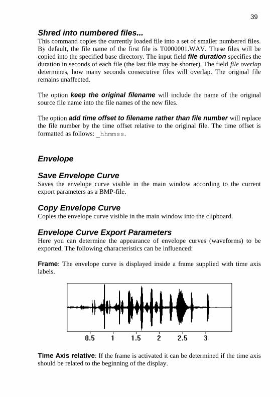
39

Shred into numbered files... This command copies the currently loaded file into a set of smaller numbered files.

By default, the file name of the first file is T0000001.WAV. These files will be

copied into the specified base directory. The input field file duration specifies the

duration in seconds of each file (the last file may be shorter). The field file overlap

determines, how many seconds consecutive files will overlap. The original file

remains unaffected.

The option keep the original filename will include the name of the original

source file name into the file names of the new files.

The option add time offset to filename rather than file number will replace

the file number by the time offset relative to the original file. The time offset is

formatted as follows: _hhmmss.

Envelope

Save Envelope Curve Saves the envelope curve visible in the main window according to the current

export parameters as a BMP-file.

Copy Envelope Curve Copies the envelope curve visible in the main window into the clipboard.

Envelope Curve Export Parameters Here you can determine the appearance of envelope curves (waveforms) to be

exported. The following characteristics can be influenced:

Frame: The envelope curve is displayed inside a frame supplied with time axis

labels.

Time Axis relative: If the frame is activated it can be determined if the time axis

should be related to the beginning of the display.

40

Time Scale: If no frame is activated you can enable a time scale below the

envelope curve.

High Resolution: The envelope curve is exported with higher resolution

compared to the screen display.

Launch separate Curve Window This command launches a separate curve window for more detailed measurements

and advanced export facilities.

Real Time Spectrum This menu option activates the Real Time Spectrum window. (see page 201)

Don’t work on copies of opened .wav files If this option is activated, all editing operations will be made on the original file

(not on a copy of it). This will accelerate opening large files. However, because

editing is applied to the original file, care must be taken not to cause unwanted

modifications to the sound file. With this option activated, the command File/Save

is not required. For files other than .wav, this option has no effect.

Georeference .wav files This command allows to link .wav sound files (that have been recorded in the field

by using a solid-state or hard disk recorder) to the geographic coordinates acquired

by a GPS receiver. This is done by comparing the time-stamp information stored in

the sound files with the tracklog or waypoint data collected by the GPS receiver.

The tracklog and waypoint data must be provided in the universal GPS exchange

format (.gpx) or the NMEA format (.txt). Most handheld GPS receivers (for

instance Garmin, Magellan or Holux GPS data logger) provide software tools for

exporting their track data into such .gpx files. The results of the geo-location

procedure are saved as waypoints or tracks into a .gpx or .kml file, which can be

displayed for instance on Google Earth. The names of the waypoints and tracks

refer the corresponding sound files. This enables a quick overview on the locations

at which the individual sound files have been recorded.

41

For a successful georeferencing procedure it is necessary that the internal clock of

the recorder is set precisely to the GPS time and that the GPS receiver is set to the

automatic tracklog mode. Alternatively, waypoints could be saved manually at

each location at the time of recording.

Input

.wav file directory: Enter or select (through the … button) here the directory that contains the recorded

.wav files. The directory can alternatively be selected by dragging one of its files

into the dialog box.

.wav file time stamp options use the date created / date modified as time stamp if there is no BWF (bext chunk) OriginationDate This option allows to select the time stamp source that should be used for the

analysis if there if there is no time stamp in the file BWF .wav file header. lf the

selected .wav files still reside on the original digital media (the CF or SD card of

the recorder), then you might use both options. However, if the files have been

moved to another media (computer harddisk), the date created usually represents

the date at which the files were copied. So, you have to use the date modified

option in this case. The software will automatically take the file duration into

account, so that the file start time can still be estimated properly.

recorder time zone: Enter here the local time zone offset (+ daylight saving time offset) of the recorder

clock in order to match the recorder time to the GPS UTC time. In case the file

system of the recorder already takes the time zone offset into account, select the

zero offset option “GMT”.

Time stamp correction: In case the recorder time has not been set properly or if the local time of the

recorder does not match the GPS time, it can be corrected here. The entered hours,

minutes and seconds are added to the ,wav file time stamp before they are

compared with the GPS log. It is therefore allowed to enter negative values.

Time stamp tolerance: The time stamp tolerance defines the maximum time interval that is accepted

between the sound file time stamp and the nearest tracklog entry. Files with time

stamps that do not meet this criterion will be ignored.

42

use the custom Avisoft Bioacoustics .wav file GPS chunk If activated, the GPS coordinates will be read from the custom GPS chunk in the

.wav file header. Use this option for .wav files that have been recorded with

Avisoft-RECORDER software.

GPS Waypoint / Tracklog File (.gpx, .kml, tcx or NMEA .txt) Select here the tracklog file from which the time stamps and GPS coordinates

should be taken. Supported file formats are the GPS exchange format (.gpx),

Google Earth (.kml with MultiTrack entries), Gamin Trainings Center (.tcx) and

NMEA 0183 formatted text log files (.txt). The NMEA option currently supports

only the $GPRMC sentence. The tracklog file can alternatively be selected by

dragging it into this dialog box.

Output

GPS Waypoint / Track File Enter here the destination .gpx or .kml file name into which the geo-referencing

results should be written. The desired file format (.gpx or .kml) can also be

selected from the corresponding list box.

create individual log files for each .wav file If this option is activated, an individual log file will be created for each .wav file.

Except of the file type extension, the file and path names of the log files will be the

same as the corresponding .wav files.

create track if distance > xxx m If the position changes while recording a sound file by more than this limit, a track

representing the path of the moving recorder will be added to the .gpx file.

add additional waypoints at xxxx sec intervals This option will create additional waypoints along the above track in order to

simplify the orientation within the .wav file.

Add additional HTML links to the .wav files This option (only available with .kml output files) will add direct HREF links

pointing to the .wav files. The original pathname of these links can be replaced by

a user-defined path (or an URL pointing to a website).

write GPS stamp into .wav file header (GPS chunk and bext Desc) This option will save the determined GPS coordinates (and GPS time) also into the

header of each .wav file. The information is saved both into the application-

specific ‘GPS ‘ chunk (that can only be read by the Avisoft-SASLab Pro software)

and the Description field of the BWAV bext chunk. If there is already a

43

description, the GPS information will be appended. If the .wav file does not

already include a bext chunk, then it will be appended to the end of the file.

launch GIS application If activated, the program will run the specified GIS (Geographic Information

System) application with the resulting .gpx/.kml file as a command line argument.

One possible program would be GoogleEarth, which can (in the current version

5.1) however only open .kml files as a command line argument. .gpx files must be

instead opened separately.

Default! This button sets all parameters to their defaults.

If the program cannot find any tracklog entry that matches the calculated UTC time

stamp of a particular .wav file, then a log file is launched that lists the UTC .wav

file time stamp (calculated from the original .wav file time stamp, the selected

recorder time zone and the time stamp correction) and the type of time

stamp used (‘crea’ = date created taken from the file system, ‘modi’ = date

modified taken from the file system, ‘bext’ = origination date taken from the BWF

(bext) file header). This information can help to properly adjust the time zone and

time stamp correction settings.

Edit title Launches an edit box for inputting a title for the sound file. This title will be saved

into the .wav file header and may be displayed on the spectrogram images.

New Instance A new instance of Avisoft-SASLab Pro is launched. Multiple instances of the

program can be used to process several sound files simultaneously.

Marking time sections A subsection of the loaded sound file can be marked by clicking at the desired start

point and dragging the cursor to the end point. Once a section has marked, this

marker can be resized by dragging the margins of the section. The whole marker

can be shifted by clicking inside the marked section and dragging it away.

Removing of the marker can be done by the menu ”Tools”/”Remove Marker”.

The parameters of the marker (t1: begin, t2: end, dt: duration) are displayed in the

unit seconds on the right of the window.

44

Analyze

Create spectrogram

The optional spectrogram overview display in the main window is only intended

for better navigation through the sound file. For this reason there is an extra

window for spectrogram display. Inside this spectrogram window spectrograms

can be exported to other applications or spectrogram structures can be measured by

different cursors.

After marking the desired section for spectrogram display you can start

spectrogram computation by the menu "Analyze/Create Spectrogram". If no

section is marked, a spectrogram of the entire sound file is generated. Note that this

procedure may take a very long time, depending on the file size and the parameters

selected. The parameters for spectrogram generation can be defined in the menu

"Analyze/Spectrogram-Parameter".

Spectrogram-Parameters

The spectrogram parameters determine the resolution in

time and frequency axis. The frequency resolution

(corresponding to the filter bandwidth of analogue

spectrographs) is determined by the sampling

frequency, the FFT length, the frame size and the

window type. The bandwidth of a spectrogram should

be adapted to the signals to be analyzed. The inverse of

the bandwidth determines the temporal sensitivity of the

spectrogram.

The following parameters can be influenced:

Frequency Resolution

FFT Length One half of the selected value corresponds to the spectrogram height. High values

result in high frequency resolution and low time resolution. For normal

applications an FFT length of 256 points should be used. The usage of 1024 points

is only useful if a high-resolution display driver (1024*768) is installed.

45

Frame size The frame size determines the percentage of the FFT

length that is actually used for the spectrum

computation (zero-padding). Low values will result

in a higher time resolution. This is accompanied by

lower frequency resolution. A frame size of 100% is

recommended for normal applications.

Window The evaluation window determines the suppression

of the unwanted spectrum distortion (so called “side

lobes” that are associated with the analysis of stationary signals) and the analysis

bandwidth. The available window types are Rectangle, Hamming, Hann,

Blackman, Bartlett (triangle), FlatTop, KaiserBessel and Gauss. The FlatTop or

Hamming windows provide the best results in most cases. The FlatTop window

provides a “flat top” band-pass filter characteristic that is ideal for taking precise

magnitude measurements.

Rectangle

Hamming

Hann

2 4 6 8 10

V

00.20.40.60.81.0

ms

2 4 6 8 10

V

00.20.40.60.81.0

ms

2 4 6 8 10

V

00.20.40.60.81.0

ms

frame size = 100%

FFT length

frame size = 75%

frame size = 50%

zero padding

46

Blackman

Bartlett

FlatTop

Kaiser-Bessel

Gauss 3.0

Bandwidth The bandwidth depends on all three parameters (FFT length, Frame size, Window)

and the sampling frequency of the sound file. In contrast to the resolution, the

bandwidth is the true physical filter bandwidth, which is usually larger than the

resolution.

Resolution The frequency resolution depends on the FFT length and the sampling frequency of

the sound file. In contrast to the bandwidth, the frequency resolution corresponds

to the height of one pixel of the spectrogram (frequency bin width = sample rate /

FFT length).

2 4 6 8 10

V

00.20.40.60.81.0

ms

2 4 6 8 10

V

00.20.40.60.81.0

ms

2 4 6 8 10

V

00.20.40.60.81.0

ms

2 4 6 8 10

V

00.20.40.60.81.0

ms

2 4 6 8 10

V

00.20.40.60.81.0

ms

47

LPC The LPC option activates an additional Linear Prediction Coding procedure that is

applied to the waveform before calculating the spectrogram. The LPC analysis

option creates a smooth spectral envelope that indicates the major energy peaks. In

primate vocalization analysis, it can help to track the formant characteristic. The

number of the prediction coefficients determines the accuracy of the resulting

smooth spectral envelope. The implemented LPC algorithm is based on the least-

square estimation technique by using autocorrelation. peak-to-peak amplitude This option determines the broad-band peak-to-peak amplitude within the FFT

frame and outputs this amplitude at the frequency bin that corresponds to the peak

frequency of the FFT spectrum. All other frequency bind of the spectrum will be

set to zero. Use this option to measure the amplitudes of very short pulses that

would otherwise be averaged out (rejected) by the FFT.

Temporal Resolution Overlap The spectrogram is generated by repeatedly computing of spectra of a sliding

window through the time data. The overlap is the step width between two neighbor

spectra. Rising overlap values result in higher time resolutions. An overlap of 50%

is recommended for most applications. Note that high values for overlap do not

increase the visible information in the spectrogram if the frame size is not reduced

in an equivalent way. The relation between frame size and overlap is displayed

graphically on the top of the window.

2

4

kHz

bandwidth

frequency resolution

temporalresolution

dimensions of a singlespectrogram pixel

1/bandwidth

48

1/Bandwidth This is the reciprocal of the bandwidth or time constant.

Resolution The temporal resolution is the width of a pixel of the spectrogram. The true

physical time constant may be different (depending on the selected parameters)

from this resolution.

fix When this option is activated and the FFT length parameter is modified, the

Overlap parameter will be altered automatically in order to keep the temporal

resolution fixed.

peak freq. interpol. The peak frequency detection in the spectrogram window is based on a maximum

search on the spectra. In order to increase the precision of the peak frequencies

beyond the spectrogram resolution, an interpolation algorithm is used. This

parameter determines the number of points used for interpolation. The option none

will inhibit the interpolation, which means, that the peak frequency resolution is

equal to the spectrogram resolution. The option auto will select the optimal number

of interpolation points for a given bandwidth.

take channel # In multi-channel files, this option determines, from which channel the spectrogram

will be generated. In stereo files the left channel is channel # 1.

Post-processing

The following optional post-processing procedures are applied to the spectrogram

generated using the parameters selected above. They do not increase the frequency

or temporal resolution. The enlarge and smooth option can be used to improve the

appearance of printed spectrograms.

enlarge image by

The spectrogram image is enlarged by the specified factor. This option is

equivalent to the menu ”Tools”/”Enlarge image” in the spectrogram window.

smooth image

The spectrogram image is smoothed. This option is equivalent to the menu

”Tools”/”Image Filter: Average” in the spectrogram window.

enable waveform editing This option enables the use of the spectrogram window command Tools/Remove

erased spectrogram sections from waveform.

49

Window This button will show a detailed graphical display of the selected Evaluation

Window.

Selectivity

This button will show a detailed graphical display of the frequency selectivity of

the selected Evaluation Window.

Threads This list box determines the number of threads that are being used for calculating

the spectrogram both on the main and the spectrogram window. When running the

software on a multicore processor, the selected number of threads should be at least

equal the number of cores (or processor threads) in order to speed-up the

calculations. Depending on the capabilities of the specific computer (such as the

hard drive data transfer rate for instance), multithreading can also be slower than

the single-thread mode. In that case, a thread number of 1 should be selected.

wait If more than one thread has been selected and this option is not activated, the

spectrogram window will be launched before the spectrogram has been completed,

which can accelerate the workflow. However, this may also lead to problems in

conjunction with the Automatic Parameter Measurements tool.

init When the above wait option is not activated, the ini option will indicate the

uncompleted parts of the spectrograms by well-defined pattern. This initialization

will however consume additional time.

Apply Use this button to re-calculate the spectrogram using the current settings without

closing the dialog box. This may accelerate the process of finding the best

parameter settings.

Default Sets the standard values for each parameter.

Spectrogram Overview For better navigation through the loaded sound file a spectrogram can be displayed

below the envelope curve display in the main window. This spectrogram can be

activated by the menu "Analyze/Overview" or the button. Note that displaying the

spectrogram needs more time for redrawing the window than without it.

50

Overview Parameters

The menu "Analyze/Overview-Parameter" can be used for selecting the display

parameter of the overview spectrogram. It can be chosen between black&white and

color display. In black&white display mode the threshold for spectrogram display

can be adjusted. In color mode the intensity of the spectrogram can be adjusted.

This is done by inputting a numerical value between zero and hundred or by

shifting the vertical scroll bar. In color mode you can select different color tables

and gradation tables.

The frequency resolution of the spectrogram can be defined by the following

parameters:

FFT Length (One half of this value corresponds to the spectrogram height.),

Frame Size (Defines the percentage of the FFT Length that is actually filled

with the waveform data.),

Evaluation Window (Determines the suppression of spectrum distortion.

Hamming window is the best choice in most cases.).

These parameters influence also the time resolution of the spectrogram. Higher

frequency resolution is accompanied with lower time resolution. Time resolution is

also influenced by the current window size and the zoom adjustment.

The combo-box titled y-scale enlargement allows enlarging the y-dimension of the

spectrogram.

In large sound files displayed at a low temporal resolution, the default fast mode

option will only display selected sample spectra out of the large file (with regular

gaps between them), which means that short sounds may be hidden on the

spectrographic overview display. If this option is unchecked, a continuous

spectrogram is internally calculated (which may be time-consuming) and the

spectral envelope will be displayed on the screen. To accelerate this kind of

spectral envelope display, the option “Optimize waveform and spectral envelope

overviews” on the File Open Dialog box can be activated.

The float FFT option will calculate the spectrogram using floating point

arithmetic, which provides more accurate spectrograms with a better signal-to-

noise ratio.

In multichannel files, the Show Channels section allows to select the individual

channels that should be displayed on the overview window. Channels that are not

selected will be hidden.

51

Apply spectrogram window parameters Applies the spectrogram parameter settings (including FFT overlap) made for the

spectrogram window to the main window overview display.

Normalize Envelope Curve This menu option controls the scaling of the envelope curve displayed in the main

window. If this option is checked the envelope curve is fitted into the display

window. This allows better observation of soft sound signals. Please note, that the

sound file itself will not be influenced.

Show Y axis grid This option enables a Y axis grid and the associated labels.

Frequency cursor This option activates a horizontal frequency cursor for measuring frequencies.

Step waveform display mode This option enables the step display mode on the (high temporal resolution)

graphic representation of the waveform:

activated:

not activated:

Fast Envelope Curve display Toggles between fast and correct envelope curve display. If this option is checked,

the display is completed faster. However, in large files under-sampling may occur.

Time axis format The Time Axis Format dialog box allows to define the format of the time axis:

show sample index instead of time units : If this option is activated, the x

axis will show the sample index instead of time units [s].

hh:mm:ss.sssss :This option activates the clock time display mode

(hh:mm:ss.sssss) instead of the continuous display mode in seconds (ssss.sssss).

52

absolute clock time : In the clock time display mode (hh:mm:ss.sssss

activated), this option adds the absolute time of day time to the time scale. There

are a number of options for getting this absolute time-of-day offset:

time file created : The time offset is taken from the file systems date creation

entry.

time file modified : The time offset is taken from the file systems date modified

entry. Note that the absolute precision of the time offset will be limited by the

available resolution of the file created/modified time and the properties of the

recording device.

Broadcast WAVE bext origination time : The time offset is taken from the

Broadcast WAVE bext chunk (origination time entry).

Broadcast WAVE bext timecode : The time offset is taken from the Broadcast

WAVE bext chunk (time reference or timecode).

RECORDER software time stamp : The time offset is taken from the custom

.wav file header entry created by the Avisoft RECORDER software. This option

ensures a sample-precise time scale within a single monitoring session.

LANC time code on USG DI (LSB) : The time offset is taken from a serial

LANC time code signal that is stored on the USG DI track of the .wav file

(recorded by using one of the UltraSoundGate units). This mode of operation

requires that the LANC time code provided by a camcorder has been recorded into

one of the DIN inputs of the UltraSoundGate. This setup allows to precisely

synchronize the .wav file with video recordings. The LANC signal is provided by a

number of SONY camcorders on their LANC socket (which is usually a 2.5mm

stereo TRS connector or in newer models a 10-pin A/V terminal jack). Note that

not all models actually provide valid time stamps on their A/V jack. This signal can

be fed into the UltraSoundGate DI input by using a custom-made interface cable

that has a 3-pole 2.5 mm TRS plug at one end (with the ring pin left unconnected )

and a 2-pole 2.5 mm TS plug at the other end. Such a cable is available from

Avisoft Bioacoustics.

SMPTE timecode on an analog channel, SMPTE timecode on USG DI (LSB) The time offset it taken from a SMTPE timecode signal that is stored either

on an analog channel or on an USG DI track. A suited SMPTE to USG DIN

adapter cable is available from Avisoft Bioacoustics.

clock reference pulses on USG DI (LSB) : The time offset is calculated from

the number of reference pulses on the USG DI track. It is assumed that the interval

53

of the external reference pulses is equal to one of the following values (allowing a

deviation of +-10% relative to the internal sample clock):

1s, 500ms, 250ms, 100ms, 50ms, 25ms, 10ms, 5ms, 2.5ms, 1ms

The detected interval will be displayed (expressed in pulses / sec) in this dialog box

once the OK button has been clicked. The option rising slope will use the rising

slope (low-high transition) instead of the default falling slope (high-low transition)

as the reference point.

Song Meter time stamp : The time offset is taken from the custom .wav file

header entry (sub-chunk “wamd”) created by Song Meter © recorders of Wildlife

Acoustics, Inc.

channel : This list box defines .wav file channel from which he LANC or SMPTE

time code signal is taken.

ADC pipeline delay : Some analog-to-digital converters (such as those in the

UltraSoundGate product family) introduce a pipeline delay relative to the digital

inputs, which can be compensated here. The edit field allows entering the pipeline

delay expressed in the number of samples. In the UltraSoundGate hardware, the

delay is usually 20 samples.

One-dimensional transformations This menu supports additional display options and transformation types of the

marked sound file section. The results of these transformations will be displayed in

a separate curve window. The following functions are available:

Time signal The fine structure of the time signal is displayed. This display allows in contrast to

the envelope display inside the main window a high-resolution observation and

measuring of time signals.

Amplitude spectrum The magnitude spectrum (y-unit [V]) of the marked section is computed. The

resolution of the spectrum is proportional to the length of the marked section. (long

term spectrum)

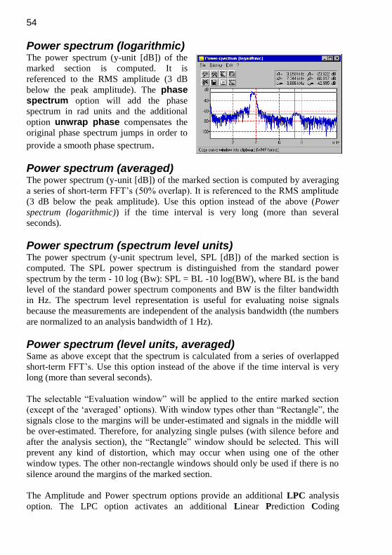
54

Power spectrum (logarithmic) The power spectrum (y-unit [dB]) of the

marked section is computed. It is

referenced to the RMS amplitude (3 dB

below the peak amplitude). The phase spectrum option will add the phase

spectrum in rad units and the additional

option unwrap phase compensates the

original phase spectrum jumps in order to

provide a smooth phase spectrum.

Power spectrum (averaged) The power spectrum (y-unit [dB]) of the marked section is computed by averaging

a series of short-term FFT’s (50% overlap). It is referenced to the RMS amplitude

(3 dB below the peak amplitude). Use this option instead of the above (Power

spectrum (logarithmic)) if the time interval is very long (more than several

seconds).

Power spectrum (spectrum level units) The power spectrum (y-unit spectrum level, SPL [dB]) of the marked section is

computed. The SPL power spectrum is distinguished from the standard power

spectrum by the term - 10 log (Bw): SPL = BL -10 log(BW), where BL is the band

level of the standard power spectrum components and BW is the filter bandwidth

in Hz. The spectrum level representation is useful for evaluating noise signals

because the measurements are independent of the analysis bandwidth (the numbers

are normalized to an analysis bandwidth of 1 Hz).

Power spectrum (level units, averaged) Same as above except that the spectrum is calculated from a series of overlapped

short-term FFT’s. Use this option instead of the above if the time interval is very

long (more than several seconds).

The selectable “Evaluation window” will be applied to the entire marked section

(except of the ‘averaged’ options). With window types other than “Rectangle”, the

signals close to the margins will be under-estimated and signals in the middle will

be over-estimated. Therefore, for analyzing single pulses (with silence before and

after the analysis section), the “Rectangle” window should be selected. This will

prevent any kind of distortion, which may occur when using one of the other

window types. The other non-rectangle windows should only be used if there is no

silence around the margins of the marked section.

The Amplitude and Power spectrum options provide an additional LPC analysis

option. The LPC option activates an additional Linear Prediction Coding

55

procedure that is applied to the waveform before calculating the spectrogram. The

LPC analysis option creates a smooth spectral envelope that indicates the major

energy peaks. In primate vocalization analysis, it can help to track the formant

characteristic. The number of the prediction coefficients determines the accuracy

of the resulting smooth spectral envelope. The implemented LPC algorithm is

based on the least-square estimation technique by using autocorrelation.

Octave Analysis The octave spectrum (y-unit [dB]) of the marked section is computed by using a set

of (FIR) octave filters complying with the ANSI S1.11-2004 standard. The output

of the filters is linearly averaged and represents the mean RMS level. The min center frequency [Hz] list box defines the lowest octave filter. The maximum

filter center frequency is determined by the sample rate of the sound file. The

option include total band power adds the RMS level of the unfiltered signal to

the end of the octave spectrum.

Third-Octave Analysis The third-octave spectrum (y-unit [dB]) of the marked section is computed by

using a set of (FIR) 1/3 octave filters complying with the ANSI S1.11-2004

standard. The output of the filters is linearly averaged and represents the mean

RMS level. The min center frequency [Hz] list box defines the lowest third-

octave filter. The maximum filter center frequency is determined by the sample

rate of the sound file. The option include total band power adds the RMS level

of the unfiltered signal to the end of the third-octave spectrum.

Autocorrelation The autocorrelation function (ACF) of the marked section is computed. The ACF

supports the recognition of periodical or correlated components in a signal.

Cepstrum The Cepstrum of the marked section is computed. The Cepstrum is computed by

determination of the inverse FFT of the logarithm of the power spectrum. Cepstral

analysis supports the separation of several multiplied signal components (for

instance in human speech).

Cross-correlation (stereo) The cross correlation (CCF) between the left and right channel of the marked

section of a stereo signal is computed. The CCF can be used for recognition of

correlations between two channels. By using of two separated microphones the

time delay of a noise signal can be determined by searching the maximum of the

CCF.

56

Cross-correlation (2 files) The cross correlation (CCF) between the marked section and the contents of the

clipboard is computed. This requires, that the clipboard has been loaded with the

signal to be compared (Menu EDIT/COPY). This kind of CCF can be used for

observation of similarities between two sound files.

Transfer function (2 stereo channels) This menu allows the determination of the frequency response of a system using

Fourier transformation. The system input has to be supplied with a white noise

signal. The left channel of the sound card has to be connected with the system

input. The right channel has to be connected with the system output. After data

acquisition is finished (a few seconds are sufficient) and a section has been marked

the computation of the transfer function is started. Note, that the marked block

must be longer than the selected FFT size. If the marked section is longer, than

several frequency responses are averaged. This will increase the precision, but the

computing time is rising. This computation method of the frequency response

delivers exact results only at those frequencies, where the magnitude of the input

signal is high enough. For this reason, those spectral lines of the frequency

response that don't exceed a threshold within the input spectrum are suppressed in

the display window. This threshold can be changed by the slider on the right of the

display window. This method of displaying allows using test signals, which don't

have a continuous spectrum. You could use a rectangle signal, where you can

obtain valid values only at the frequencies f0, 3f0, 5f0, ... .

Because of the algorithm used ( |G(f)|=|Sxy(f)|/|Sxx(f)| ) the frequency response is

precise even if there are noise sources within the system.

Frequency response, sine sweep mono This command computes the frequency response of a system from a sine sweep

test signal passing the system. It is assumed, that the test signal (sine wave with

varying frequency and constant amplitude) is fed into the input of the system

without distortion. The sine sweep altered by the system is then analyzed by

consecutive short-time FFT’s. The maximum amplitude and the frequency of that

maximum are extracted from each block. The result is a frequency response plot

showing amplitude against frequency. The plot is normalized relative to the

maximum amplitude. The ‘Evaluation window’ determines the precision of

amplitude measurements. The FlatTop window is recommended for optimal

results. The FFT size determines the precision of frequency measurements. High

values provide more precise frequency values. However, high values will reduce

the number of amplitude samples (each FFT block supplies one amplitude sample),

which requires longer and slower frequency modulated test signals. An FFT size of

512 in conjunction with a test signal sweeping from 0 to the Nyquist frequency

within 20 seconds is recommended. The sine sweep test signal can be generated

using the command Edit/Synthesizer/dialogue.

57

The Increment listbox defines the frequency axis sampling method. The default

option adaptive will create a sample for each of the FFT spectra, while the other

frequency options will output only provide a limited number of samples depending

on the selection.

Frequency response, sine sweep stereo This command computes the frequency response of a system from a sine sweep

test signal passing the system. In contrast to the command above, the test signal is

sampled at both input and output of the system (using left and right channel of a

soundcard). The amplitude samples taken from the output are divided by those

taken from the input. This method eliminates eventual precision degradation

caused by nonlinear test signals (varying amplitude depending on frequency).

Therefore this command should also be used, if it is impossible to feed the test

signal into the input of the system without frequency response distortion. In case

the amplitude of the test signal is decreased by the system dramatically, an

additional amplifier might be necessary. For parameter settings see the command

Frequency response, sine sweep mono, described above.

Histogram The histogram of the samples occurred inside the marked section is computed. The

number of classes can be defined in dependence of the sound file resolution (bit-

count). The histogram display can be used for the evaluation of the quality of the

analog to digital converter.

XY Plot The amplitudes of two channels are plotted against each other.

XYZ Plot The amplitudes of three channels are plotted against each other

Impulse Density Histogram The time intervals between short signal impulses are displayed in a histogram. The

detection of the signal impulses is done by a threshold comparison of the envelope

of the time signal. For the adaptation of the algorithm to the signal to be analyzed

several parameters can be adjusted:

Threshold: The threshold is defined as a percentage of the maximum of the envelope. If the

envelope exceeds the threshold, an impulse is recognized.

Delay: Because the signal impulses have certain duration and the multiple recognition of

the same impulse is undesired, a delay time is required. When the beginning of an

58

impulse has been recognized, no further impulse is recognized for the delay-time,

even if the threshold is exceeded. The delay should be a little bit longer than the

maximum impulse-width in order to prevent multiple recognition’s of the same

impulse. Note, that close impulses cannot be recognized if the delay is too long!

Resolution: The resolution determines the time raster for the acquisition of the impulse density

histogram.

Impulse Rate The time intervals between short signal impulses are displayed. The detection of

the signal impulses is done by a threshold comparison of the time signal. For the

adaptation of the algorithm to the signal to by analyzed several parameters can be

adjusted:

Threshold: The threshold is defined in percent of the maximum of the envelope. If the time

signal exceeds the threshold, an impulse is recognized (slope based).

Delay: Because the signal impulses have certain durations and the multiple recognition of

the same impulse is undesired, a delay time is required. When the beginning of an

impulse has been recognized, no further impulse is recognized for the delay-time,

even if the threshold is exceeded. The delay should be a little bit longer than the

maximum impulse-width to prevent multiple recognitions of the same impulse.

Note, that close impulses cannot be recognized if the delay is too long!

Lorenz plot The Lorenz plot (also called phase space display) displays the time intervals

between three consecutive pulses in a 3D display. This kind of display may be

useful for evaluating the randomness of pulse intervals. In constant pulse rates the

Lorenz plot will display all pulses at the same location. In constantly rising or

falling pulse rates, the pulses will be displayed along a straight line in 3D space. If

the pulses are more randomly spaced, the consecutive pulses will be displayed at

larger distances from each other within a larger cloud in the 3D space. The

algorithm for the impulse interval measurement is the same as described for the

Impulse Rate function above.

59

Envelope (analytic signal) The envelope of the marked section is computed. This is done by the analytical

signal method using Hilbert transformation. This method allows a more precise

result as the envelope display in the main window.

Instantaneous frequency The instantaneous frequency of the marked section is computed using the

analytical signal method with Hilbert transformation and differentiating filter. The

duration of the marked section is limited to 65536 samples.

For isolation of separated signal sections the instantaneous frequency is displayed

only if the envelope of the signal exceeds a certain value. This threshold is defined

in percent of the maximum value of the whole envelope. The scroll bar on the right

of the curve window allows the adjustment of the threshold.

Especially for analyzing of fast changing sine-signals this method is advantageous

compared to a spectrographic representation.

Zero-crossing analysis A zero-crossing analysis of the marked section is carried out. The duration of the

marked section is not limited. The parameter Resolution determines the temporal

resolution of the output curve. The combo-box Average over allows selecting the

method of averaging. By selecting the first entry (which corresponds to the

Resolution edit field), the zero-crossing measurement will be averaged over that

time. By selecting one of the following entries (x cycles), the measurement will be

carried out over the specified number of cycles. In that case an appropriate

Resolution values should be chosen, so that temporal details will not be lost.

The implemented zero-crossing algorithm uses linear interpolation to increase the

frequency resolution.

For isolation of separated signal sections the zero-crossing analysis is displayed

only if the envelope of the signal exceeds a certain value. This threshold is defined

in percent of the maximum value of the whole envelope. The scroll bar on the right

of the curve window allows the adjustment of the threshold.

Root mean square (linear) / (logarithmic) The root mean square of the marked section is computed. The desired averaging

time can be defined in the edit field "Averaging time". You can select the standard

values FAST (125ms) or SLOW (1000ms) using the push buttons F and S. The

option field "exp." determines if the averaging should be done exponentially

(recursive) with the specified averaging time as time constant or arithmetically

over the averaging time. The root mean square can be displayed linear or

60

logarithmic. For sound level measurements in dB the logarithmic root mean square

should be used.

Envelope The amplitude envelope of the marked section is computed. This is done by the

following algorithm: The envelope follows the rectified waveform when its

amplitude increases. When the input level falls, the envelope decays with the

specified time constant, which will bridge valleys of the signal. The time constant

should be adapted to the signal to be analyzed.

Gate function This function can be used to analyze the temporal pattern of sounds. The amplitude

envelope (see function above) is compared to a threshold level. The gate function

will be 1 where the amplitude envelope exceeds the threshold, and it will be zero

elsewhere. The threshold is specified in percent of the maximum amplitude

(measurement range). In order to tolerate short amplitude gaps or noise bursts, the

gate function output will only change when the internal state of the gate function is

stable for a predefined minimum time interval (the Delay parameter). For proper

operation, the Delay parameter must be smaller than the minimum total duration of

the pulses. The Delay parameter will also influence the time resolution of the gate

function.

Gate function (signal/silence duration) This function is similar to the gate function above. The only difference is the

format of the output. In contrast to the above gate function that represents the

output as a time-continuous sequence of ones and zeroes, this option returns the

durations of the signal events and the preceding silent periods. The y-values (pulse

durations) are positive for signal events, and negative for silent periods between

signal events. So the output is an alternating sequence of positive event durations

and negative inter-event durations, where the x-axis represents the index of the

events.

Gate function (interpulse interval) This function is similar to the Gate function (signal/silence duration), except that it

provides the total time intervals between the beginnings of consecutive pulses

(interpulse interval). This function is comparable to the Impulse rate function that

uses a simple amplitude threshold instead of the more complex gate operation for

measuring the interpulse intervals.

61

Pulse Train Analysis

The Pulse Train Analysis option allows measuring the temporal parameters of

waveforms automatically. That includes both simple counting of sound pulses or

calls and even more complex measurements as interpulse intervals and pulse group

analysis. There are various envelope tracking and pulse recognition algorithms that

can be selected depending on the type of signals to be analyzed.

Basically, the Pulse Train Analysis procedure consists of the following stages:

1. Generating the envelope of the waveform,

2. Pulse detection,

3. Post filtering (optionally rejecting gaps and short pulses)

4. Pulse counting, Measuring interpulse intervals, durations, amplitudes and

time stamps

5. Group analysis for identifying pulse groups that are separated from each

other by larger intervals.

The Pulse Group Analysis function is usually launched from the main window

command ‘Analysis’/’Pulse Train Analysis…’. The analysis can be limited to a

subsection the entire sound file by marking a section before executing the Pulse

Group Analysis command.

Alternatively, the Pulse Train Analysis suite can be activated from the Curve

window when it already displays an envelope (Display/Pulse Train Analysis…).

Depending on the quality of the sound recordings it might be necessary to high-

pass filter the waveform before applying the Pulse Train Analysis (main window

command Edit/Filter/Time Domain IIR Filter…). This procedure would remove

irrelevant low-frequency noise that might otherwise prevent a proper envelope

analysis. Similarly, it is possible to run the Pulse Train Analysis directly on a

spectrogram slice taken from the spectrogram window (first activate

Display/Additional Spectrogram Information/Time axis/’Single frequency’ or

‘Frequency Interval’ and then transfer the frequency slice into the curve window

by double-clicking at the graph or via File/Data Export/’Copy Envelope into Curve

window’.

The envelope of the currently loaded sound file and the detected sound pulses will

be displayed in a separate Curve window. Additionally, a Pulse Train Analysis

panel is launched. It allows adjusting the analysis settings and displays the results

numerically. For the successful application of the Pulse Train Analysis feature it is

essential that the analysis parameters (time constant, threshold, …) and the analysis

methods have been selected properly. Usually, it is required to optimize the

settings interactively until the desired behavior is reached.

62

Settings…

This dialog box allows selecting the available pulse train analysis methods and the

desired measurements.

Methods

Envelope This list box offers the available envelope calculation methods. Any quantitative

analysis of waveforms requires some kind of amplitude envelope detection. For the

temporal analysis of waveform patterns, it is usually not required to look at single

oscillations on the original waveforms. So, it is appropriate to trace the outline of a

waveform only. There are several approaches for computing the envelope or a

meaningful approximation of the variation of long-term amplitude of a waveform.

Rectification + exponential decay The original waveform is first rectified (all negative samples will be inverted). The

resulting envelope follows the rectified waveform as long as the amplitude is

rising. If the amplitude of the rectified waveform decreases (negative slopes), the

most recent peak amplitude decays exponentially at a pre-defined time constant

(peak-hold mechanism). In this way, the small instantaneous amplitudes between

consecutive waves will be bridged.

Rectification + exponential decay + decimation This option is identical to the above option, except that the sample rate of the

resulting envelope will be reduced (decimation). The amount of decimation is

selected according to the time constant of the envelope computation. The final

resolution of the decimated envelope is displayed on the main Pulse Train Analysis

panel. The additional decimation decreases the temporal resolution of the final

measurements but accelerates the processing and displaying of the envelope, which

is certainly important while processing large files.

RMS + decimation The root mean square of the waveform is computed block wise (averaging over a

discrete number of samples without overlap). The inherent decimation corresponds

to the ‘time constant’ parameter. In contrast to the option ‘Rectification +

exponential decay’, this computational method does not include a peak-hold

mechanism. Consequently, short amplitude peaks will be averaged out. Therefore,

the RMS method is suited in situations where short peaks need to be rejected or are

out of interest.

RMS exponential moving average+ decimation The root mean square of the waveform is computed in a moving average mode.

The resulting envelope is decimated according to the selected time constant. . In

63

contrast to the option ‘Rectification + exponential decay’, this computational

method also does not include a peak-hold mechanism.

Original waveform (no manipulation) The original and unmodified soundfile is used for the peak search.

The Envelope method can only be selected when the Pulse Train Analysis

command has been launched directly from the main window waveform display.

The other entry points already operate on existing envelopes. The properties of

these envelopes must be set before entering the Pulse Train Analysis command

(e.g. by selecting appropriate Spectrogram Parameters if the Pulse Train Analysis

is applied to a spectral slice of a spectrogram).

Pulse detection

There are two basic methods for detecting pulses in the amplitude envelope:

Gate Function The gate function simply compares the envelope with a pre-defined, fixed

threshold. The absolute threshold level will heavily influence the number and

durations of the recognized pulses. This method is recommended for analyzing

signals that exhibit only minor amplitude variations.

Peak Search with Hysteresis Additionally to the absolute threshold, this method is based on a relative peak

detection algorithm that identifies local peaks in the envelope signal. A peak is

recognized when its peak amplitude exceeds the minimum amplitude that precedes

this peak by a predefined factor. In this way, it is possible to detect both soft and

louder peaks that could not be detected by a simple absolute threshold comparison

(Gate function). Most sound recordings contain some reverberation (short-term

echoes). That reverberation can prevent the safe separation of the single sound

pulses with varying amplitudes in simple gate function analysis set-ups. Therefore,

this method is recommended for analyzing signals that exhibit larger amplitude

variations. It is certainly useful for analyzing signals with varying amplitudes that

are additionally influenced by reverberation.

64

Measurements

The Measurements section allows selecting the measurements that should be taken.

Time : Absolute time stamp of the pulse.

Time relative to group start : In the group analysis mode, the relative time

stamp of each pulse is referenced to the first pulse of the group.

Duration : The duration is determined by the threshold settings. It is measured

from the point where the signal exceeds the threshold to the point where the signal

falls below the threshold level.

Interval : Interpulse interval between pulses, measured from the start of the

preceding pulse to the start of the current pulse.

Amplitude : The peak amplitude of the pulse. The dB option will output result in

dB units.

Peak frequency / Bandwidth / Wiener Entropy : An FFT analysis is applied

to the detected pulse in order to determine the peak (or dominant) frequency,

bandwidth or Wiener entropy. The ‘Setup…’ button launches a dialog box that

defines the spectral analysis settings:

The FFT size determines the maximum duration of the analysis frame. The

resulting Frame duration and the resulting Frequency resolution of the

currently selected FFT size is displayed.

The weighting Window is applied to the analysis frame prior to calculating the

FFT spectrum. Depending on the structure of the pulses, the specific window type

may influence the peak frequency results. The Rectangle window will not

influence the temporal structure (the location of the pulse within the analysis frame

does not matter). The other weighting functions emphasize the middle of the

analysis frame, which may distort the frequency spectrum. In case the pulses have

a distinct start and end and the analysis frame fully covers the pulses, then the

Rectangle window is recommended. In case the analysis frame is shorter than the

pulse (pulses longer than the FFT size), then one of the other weighting functions

will provide more reliable results.

65

The option ‘limit the analysis frame to the detected pulse duration’ activates a zero-padding mode. If activated and if the pulse is shorter than the

selected FFT size, then the FFT spectrum will be computed only from the detected

pulse duration. Otherwise, the actual duration of the pulse is ignored and the

spectrum is computed from the full (FFT size) frame that is centered on the

detected pulse. This option does only have an effect as long as the durations of the

pulses are determined (‘Gate function’ or ‘Peak search with Hysteresis with the

‘Duration’ activated). In case the duration is not available, spectrum will always be

computed from the full FFT size. In that case, it is also recommended to adjust the

FFT size to the durations of the pulses.

The Bandwidth Settings define the threshold for the bandwidth calculation

and the way how the bandwidth is determined. If the total option is activated, the

bandwidth will cover all peaks that exceed the threshold. Otherwise, the bandwidth

will only cover the maximum peak exceeding the threshold.

Add filename : The name of the current sound file. The related option to each row will add the filename to every row – otherwise it will only be added to the

first (pulse) row. The option with path will include the entire pathname.

Group Analysis The group analysis option allows assigning close pulses to single groups.

Time : Absolute time stamp of the group (= time stamp of the first pulse in the

group).

Pulses / Group : Number of pulses in the group.

Pulses / Sec : Pulse rate within the group (number of pulses per second).

Duration : Duration of the group (from the start of the first pulse to the end of the

last pulse).

Interval : Interpulse interval between groups, measured from the start of the

preceding group to the start of the current group.

Amplitude : The peak amplitude of the group (the maximum peak within the

group).

use section labels as groups: If this option is checked, the groups will be

defined by section labels (instead of the group time setting).

Overall Measurements

Pulse count : The total number of pulses.

Pulse rate : The total pulse rate (pulses per second) measured from the start of

the first pulse to the start of the last pulse.

Group count : The total number of groups.

66

Group rate : The total group rate (groups per second) measured from the start of

the first group to the start of the last group.

On time (absolute in sec) : The total duration of all pulses.

On time (relative in %) The total duration of all pulses divided by the time

interval from the start of the first pulse to the start of the last pulse.

referenced to the entire waveform : If this option is activated, the On time

(relative in %), Pulse rate and Group rate will be referenced to the duration of the

entire waveform (instead of the duration from the first to the last pulse).

Apply an upper amplitude limit : If activated, pulses whose peak amplitude

exceed a user-defined limit will be ignored.

Show pulse numbers If this option is activated, their number will identify the recognized pulses on the

envelope display.

Take channel # This list box selects the sound file channel on which the Pulse Train Analysis is

done.

DDE / LOG This button launches the DDE Parameters / Log File dialog box. These settings are

used for exporting the measurement results via the Copy buttons.

Default This button will reset all settings to their defaults.

time constant When the Pulse Train Analysis is launched from the main window, the envelope of

the marked section is computed automatically. The time constant for that envelope

computation can be entered here (unit milliseconds). Click at the Update button for

re-computing the envelope with the newly entered time constant. The envelope

computation method can be selected from the Settings dialog box. The value of the

time constant (and the envelope computation method) will heavily influence the

pulse train analysis results. So, that value should be adapted to the kind of signals

to be analyzed. Generally, waveforms with low pulse rates and long pulses should

be processed with larger time constants. Shorter pulses or higher pulse rates require

shorter time constants.

threshold The pulse detection is based on a threshold comparison on the envelope.

Depending on the selected pulse detection method (Settings dialog), this threshold

67

controls the pulse recognition. In the ‘Gate Function’ method, a pulse is detected

once the envelope exceeds the threshold level. In the ‘Peak search with Hysteresis’

method, any peaks that do not exceed the threshold level will be ignored (the actual

peak detection is controlled by the hysteresis parameter). The threshold level can

also be entered visually by dragging its graphic representation on the envelope

curve display. The rel. option will specify the threshold level relative (expressed in

dB) to the peak of the entire envelope curve. Use this option to compensate for

varying signal amplitudes.

hysteresis If the pulse detection method ‘Peak search with Hysteresis’ has been selected, then

the hysteresis parameter controls the peak detection (in conjunction with the

threshold parameter). The underlying algorithm searches for local peaks in the

envelope. A peak is recognized when its peak amplitude exceeds the minimum

amplitude that precedes this peak by a predefined factor. This factor that is

expressed in dB (the hysteresis parameter) should be adjusted in such a way that

the relevant peaks are still recognized, while smaller irrelevant noise peaks are

ignored. As a rule of thumb, the hysteresis parameter should be set to a value

slightly lower than the signal to noise ratio of the recording (where the

reverberation is also considered as noise). In most cases a hysteresis between 10

and 20 dB is appropriate. Please note that the pulse detection results are influenced

both by the hysteresis and the time constant of the envelope generation.

start/end threshold If the pulse detection method ‘Peak search with Hysteresis’ and the measurement

option ‘Duration’ have been selected, the start/end threshold controls the pulse

duration and time stamp measurements. This relative threshold is referenced to the

peak amplitude of each pulse. Therefore, lower values (e.g. –20 dB) will provide

longer durations than higher values (e.g. –10 dB). For internal reasons, the absolute

value of the start/end threshold parameter must be smaller than the hysteresis

68

parameter. Therefore, the start/end threshold parameter will be decreased

automatically when the hysteresis parameter becomes smaller than the start/end

threshold.

group time If the Group Analysis option has been activated from the Settings dialog, then this

group hold time parameter determines which pulses are grouped together. All

pulses that are closer than the group time parameter will be associated to a single

group. So, this parameter should be set to a value that is significantly larger than

the longest break between the pulses that should be assigned to a single group. The

group time is expected in milliseconds and applies to the time intervals between

the start of a pulse and the end of the preceding pulse. If there is no information on

the duration (method ‘Peak search with Hysteresis’ and the Duration option not

activated), then the start and end of a pulse is the same and the group time simply

applies to the inter-pulse interval.

Post filter The post filter allows to further improving the reliability of the pulse detection

mechanism. Short gaps within a sound burst can be rejected so that originally two

close pulses are treated as a single element. Similarly, single short pulses can be

rejected.

enable This check box enables the Post Filter. Certainly in conjunction with the pulse

detection method ‘Peak search with Hysteresis’, there are several parameter

settings that all influence the final pulse detection. Therefore, it is recommended to

disable the post filter until the threshold and hysteresis parameters have been

adjusted properly.

hold time The hold time controls the rejection of short gaps. Any gap shorter than the hold

time will be rejected.

pulse detection without hold time

69

pulse detection with a post filter hold time set to 16 msec

min dur. The minimum duration parameter controls the rejection of short single pulses.

Pulses shorter than the min dur. parameter will be rejected.

The hold time and min dur. entries require to confirm the modification made by

clicking at the Update! button in order to re-compute the results.

Close This button abandons the Pulse Train Analysis.

Update! This button reads the current entries from the parameter edit boxes and updates the

pulse train analysis results.

Pulse analysis results

The results of the pulse train analysis are displayed in the list box on the left. Only

those Measurements that have been selected from the Settings dialog will be listed

here.

Copy This button copies the contents of the pulse list into the Windows clipboard. The

ASCII-formatted table can then be pasted into another application (e.g. Excel).

Optionally, the data will be transferred via DDE or written into a LOG file. The

required settings can be made from the DDE / LOG button on the Settings dialog

box.

Save This button saves the list into an ASCII file.

Head The column titles of the list will be copied into the clipboard. This may help

identify the various entries in the list.

70

Label

The Create Labels dialog allows creating labels for either pulses or pulse groups.

These labels can for instance be used for a subsequent spectral analysis step within

the spectrogram window (Automatic Parameter Measurements with the ‘Element

separation’ set to ‘interactively (section labels)’).

Label text The Label text section lists all available measurements that can be copied to the

text label.

Layer The Layer list box defines the layer of the section labels.

Delete previous labels If this option is activated, all previously existing labels will be deleted.

Default This button sets all parameters to their defaults.

Overall measurements : Pulses

The Overall Measurements selected from the Settings dialog are displayed on the

right of the pulse list.

Copy The Copy button located at the top of the Pulses section will copy the above

overall measurements into the clipboard.

Group analysis results The results of the group analysis are displayed in the list box below the pulse list.

Only those Group Analysis Measurements that have been selected from the

Settings dialog will be listed here.

Copy This button copies the contents of the group list into the Windows clipboard. The

ASCII-formatted table can then be pasted into another application (e.g. Excel).

Optionally, the data will be transferred via DDE or written into a LOG file. The

required settings can be made from the DDE / LOG button on the Settings dialog

box.

Save This button saves the list into an ASCII file.

71

Head The column titles of the list will be copied into the clipboard. This may help

identify the various entries in the list.

Label This button creates a label for each recognized group. See Create Labels for

details.

Overall measurements : Groups

The Overall Measurements selected from the Settings dialog are displayed on the

right of the groups list.

Copy The Copy button located at the top of the Groups section will copy the above

overall group measurements into the clipboard.

72

Specials > Copy energy of marked section Copies the energy of the marked section into the clipboard. The energy is the sum

(integral) of the squared amplitudes multiplied by the sampling time. The unit is 1

V*V*s

Copy RMS of marked section Copies the RMS of the marked section into the clipboard. The RMS is the root

mean square. The unit is 1 Volt.

Copy peak-to-peak of marked section Copies the peak-to-peak amplitude of the marked section into the clipboard. The

unit is 1 Volt.

Time-delay-of-arrival (TDOA) measurements

It is possible to determine the position of a sound source (e.g. an animal) by means

of an array of microphones (passive acoustic location). The time differences at

which the sound signals arrive at these microphones can be computed by cross-

correlation. If the positions of the microphones are known, the position of the

sound-source can then be calculated by using a set of hyperbolic equations.

The command Copy single TDOA from marked section computes the delay

of a signal that is present in all channels by using a cross correlation technique.

Only the marked section will be used for the cross-correlation. The marked section

should cover the signal to be measured in all channels. Otherwise, the algorithm

will provide wrong results. The multi-channel sound file necessary for two- or

three-dimensional location can be created from several mono or stereo wav-files by

the Add channel(s) from file command in the “File” menu. Alternatively, multi-

channel files can be imported from external non-wav files acquired by other data

acquisition devices (see Import-Format for details).

The maximum of the cross-correlation function is searched and its position is taken

as the delay between each pair of channels.

The results of the time delay determination between all channels will be copied

into the clipboard and can be additionally transferred via DDE into a spreadsheet

application like Excel. The delays are represented as floating point numbers (unit 1

second) in the ASCII format. Tabulators separate the single values. If there are

more than two channels, the sequence of the values is as follows:

(1-2) (1-3) (2-3) (3 channels: first value is the delay between channel 1 and 2, the

second value is the delay between 1 and 3 and third value is the delay between 2

73

and 3. The first value (2-1) will be positive, if the signal arrives first in channel 1

and then in channel 2.

(1-2) (1-3) (1-4) (2-3) (2-4) (3-4) (4 channels),

(1-2) (1-3) (1-4) (1-5) (2-3) (2-4) (2-5) (3-4) (3-5) (4-5) (5 channels, and so on)

The command Copy multiple TDOA’s from section labels does the same as

Copy single TDOA from marked section, except that the computations will

be made for all section labels instead of the marked section. CR control characters

will separate the results for each label.

The option Add time stamps will add a time stamp to each TDOA data set. This

will allow to track both path and speed of the sound source. The time stamp

represents the middle of the time interval from which the TDOA has been

computed. When the following option Add duration is activated, the time stamp

represents the start of the time interval.

The option Add duration will add the duration of the underlying waveform

section from which the TDOA has been computed.

The option Add amplitudes will add the peak-to-peak amplitudes of the

underlying waveform sections from which the TDOA has been computed (order:

channel1, channel2, …).

The option Add label will add the text labels of the associated section labels from

which the TDOA have been computed. This entry will be empty for the command

Copy single TDOA from marked section.

The option Take positive CCF maximum only will search for the positive

maximum of the cross correlation function. If this option is not activated, it will

search for the maximum on the absolute magnitude values, which means that also a

negative peak can be determined as the position of the maximum correlation.

Detect waveform events and create section labels See Create section labels from waveform events, page 94.

Detect and classify waveform events

See Create section labels from waveform events, page 94 and Classify labeled

sections, page 101.

74

Scan for template spectrogram patterns

This classification command allows to identify certain spectrogram patterns by

using a spectrogram cross-correlation algorithm. The entire sound file is

continuously compared with a user-defined set of template spectrograms. The

comparison is done by computing a two-dimensional spectrogram cross-correlation

function (CCF). A subsequent peak search on the resulting CCF trace provides the

time stamps of the occurrence of the template patterns within the soundfile. The

name of the template spectrogram that provides the maximum correlation

coefficient (the highest degree of similarity) within a user-defined time interval

(masking interval) is considered as the class membership of the unknown event.

The template spectrograms that have previously been saved from the spectrogram

window command “File”/”Save Spectrogram (ASCII/Binary)…” as .son files can

be selected from the Select button or simply by drag-and-drop. The launched File

Open dialog allows to select several files at once (by using the <Shift> or <Crtl>

keys). All template spectrograms must reside in the same folder. The templates

must have been created with corresponding spectrogram parameters (same FFT

length, frame size, overlap and sample rate). Also, the sample rate of the sound file

to be examined must correspond to the sample rate at which the template

spectrograms have been created.

In order to reject low-frequency noise that might disturb the correlation procedure,

a high-pass cutoff frequency can be specified. All spectrogram components

below that frequency will be ignored. Accordingly, the low-pass cutoff frequency

setting will exclude any signal components above the specified frequency.

For tolerating slight frequency deviations between the templates and the unknown

sounds, a max frequency deviation can be specified. Depending on the frequency

resolution of the template spectrograms and the specified maximum deviation, the

cross-correlation will be repeated for various frequency shifts. The maximum

correlation coefficient is taken as the similarity score. The cross-correlation

algorithm is similar to that of the Avisoft-CORRELATOR application (see the

online help or the manual of that application of details).

The identification threshold controls the peak search on the CCF traces.

This threshold is applied directly to the cross-correlation coefficients. Sound events

that cause CCF coefficients below that threshold will be ignored. Once a peak

exceeds the threshold, it will be taken as a potential sound event of the associated

class. If you have selected more than one template spectrogram, the algorithm also

searches for peaks on the other template channels that occur shortly before and

after the original peak. If there are higher peaks on the other template channels

75

within the masking interval, the sound event will be assigned to the class that

provides the highest peak.

Slight deviations between the template spectrograms and the sound event under

question might prevent the proper recognition of its class memberships. Adding

more templates that cover as much variations as possible can compensate this

problem (at the expense of computing time). In order to get unified class names for

all variations, the filenames of the spectrogram templates (.son) that should belong

to the same class must start with identical names. The unified class names must be

separated from the rest of the filename by either a dot (.) or an underscore (_). The

following set of templates would create two classes only (e1 and e2). e1_v1 and

e1_v2 represent variations that refer to the same class.

e1_v1.son

e1_v2.son

e2_v1.son

e2_v2.con

If the option Mark detected events by labels is activated, the results of the

classification procedure will be stored into labels that are displayed on the

waveform and spectrogram displays. The option Create section labels (instead of single-point labels) will generate section labels instead of the

standard single point labels. The durations of these sections will be determined by

the durations of the associated template spectrograms. The margin parameter will

additionally dilate the section labels by the specified time interval.

The desired section label layer to which the labels should be assigned can be

selected from this list box.

The option Filter Classification Results allows to pick out a single class out of the

classified sound events (by ignoring all events that have been assigned to other

classes). The take class list box selects the desired class. The option replace label

texts with index will assign an incrementing index to the filtered events.

The Default button will set all parameters to their default settings.

The classification procedure is initiated by clicking at the Start button. A new

classification report window will appear (see page 105).

76

Edit

The menu "Edit" supplies different functions for editing the loaded sound file.

These functions can be used to remove undesired disturbance signals or to generate

artificial songs for playback experiments. These functions use a program specific

clipboard that is not identical with the Windows-clipboard.

Undo Returns to the file as it was before the last modification.

Redo Repeats the last command (except File/Open, File/Record, ...).

Copy The marked section is copied into the clipboard.

Paste The marked section is replaced by the contents of the clipboard.

Cut The marked section is removed and copied into the clipboard.

Trim The samples outside the marked section will be removed. If there is no marked

section all samples outside the visible section will be removed.

Change Volume The volume of either the marked section (apply to marker) or the labeled sections

(apply to label) is changed. The following operations are supported:

constant The marked section is changed by a constant value. The edit-box "a=" allows to

input the desired value. A factor of 2 will amplify the signal by 6dB. A factor of

0.1 will decrease the volume by 20dB. Use the dB option for directly entering dB

values.

77

In the edit box ton/off you can specify the duration of the soft transition on the

edges of the marked section. The shape of this transition can be selected in the list-

box behind (linear, sine 1/2, sine 1/4)

Normalize

The marked section will be normalized to the desired percentage of the dynamic

range. As a result the maximum of the marked section will be equal to the specified

value. In order to remove bias offset from the signal, the option ”Remove offset”

should be checked. Otherwise, bias offset, which can be caused by poor

soundcards, may distort the normalize operation.

This normalizing function can be used in order to generate comparable

spectrograms from recordings with different recording levels. FadeIn Inside the marked section the amplitude is altered continuously from zero to 100%.

The shape of tapering can be selected in the list box behind (linear, sine 1/2, sine

1/4).

FadeOut Inside the marked section the amplitude is altered continuously from 100% to zero.

The shape of tapering can be selected in the list box behind (linear, sine 1/2, sine

1/4).

(Amplitude modulation / Multiplication with) a-t ASCII-file The marked section is multiplied by the selected amplitude envelope ASCII-file

(extension ".at"). The Edit button below allows editing the selected amplitude

envelope file graphically. A new envelope can be created by specifying a new file

name (extension .at). In the appearing curve window, the envelope can be edited by

mouse drawing. Existing points can be moved by left clicking and dragging them

to a new location. A point can be removed by right clicking on it. The entire shape

can be removed by the menu option Edit/Reset Shape of the curve window.

New points are inserted by left clicking at the lines between points. In order to

enter the modifications made in the curve window, the shape must be saved by the

Save button of the Change volume dialog box.

WAV-file The marked section is multiplied by the selected WAV-file (extension ".wav").

Clipboard The marked section is multiplied by the contents of the clipboard (WAV-file).

78

Modulation freq. The marked section is multiplied by a sine shaped modulation frequency (carrier =

fc) of the specified frequency. Each frequency component (fs) of the sound file will

be split into two different frequency components with half amplitude: fc+fs, fc-fs.

Limit to

The marked section is limited to a predefined level. The option "sine" instead of

"linear" supplies a soft transition into saturation.

Divide If this option is active, the marked section will be divided by the file (instead of

multiplication). This allows carrying out normalizing operations.

Delete The marked section is deleted.

Delete with taper The marked section is deleted with a soft transition at the margins. The transition

interval (t on/off) can be defined from the command Change volume...

Insert silence A silent block is inserted at the current inserting position. The length of the

inserted block is determined by the length of the marked section.

Insert silent margins Silent sections of the specified duration will be inserted at the start and the end of

the file.

Mix The content of the clipboard is added to the signal at the current inserting position.

Take care that the signals to be added are small enough that no overflow can occur.

Reverse The samples of the marked section will be reversed.

Info about Clipboard This menu delivers information about the contents of the clipboard.

79

Single sample points can be edited by the mouse. To do this you have zoom into

the file until the single samples become visible. When moving the mouse cursor

across the horizontal lines representing the single samples the mouse cursor will

change into a vertical double arrow. By shifting that lines up or down the samples

can be edited.

80

Compress >

Remove silent sections Settings This command will remove the silent section from a sound file. Those parts of the

file those are softer than a predefined threshold will be removed from the file.

Though, the original temporal structure of the sound file is saved along with the

waveforms, which still allows measuring the original time structure. Red ticks at

the top of the waveform and spectrogram displays indicate the removed silent

sections.

The settings for this command can be made from Edit/Compress/Settings…

The sound event detection is based on a simple threshold comparison on the

rectified waveform. Silent sections that last longer than the hold time or those are

at least twice the margin will be removed. Additionally, a user-defined margin can

further dilate the preserved sections around the significant sound events. See

Create section labels from waveform events (see page 94) for details on how to

adjust these parameters (internally, the software first creates section labels for the

detected sound events and subsequently removes the gaps between those labels).

It is possible to execute this command automatically on each file that is opened in

Avisoft SASLab Pro. To enable this mode of operation, activate the option

Actions/On new sound file/Remove silent sections. A corresponding option is also

available in the Browse command (see page 22).

Back ground noise (e.g. wind noise) might prevent a proper element separation.

Therefore, it might be useful to first remove the noise (e.g. by high-pass filtering).

Remove gaps between section labels

This command will remove the gaps between the currently existing section labels.

The original time structure will be saved in the .wav file header for later re-

construction by the option Expanded view. The resulting cutting locations are

shown by short vertical marks at the top of the waveform and spectrogram display.

The command is only available for uncompressed or expanded files. Section label

input can be easily done by left clicking at the waveform / spectrogram, while the

shift key is pressed. Subsequent switching between a compressed and un-

compressed view is possible by the option Expanded view.

81

A similar, but automatic command for sound file compression is the spectrogram

window command Automatic Parameter Measurements / Remove gaps between

detected elements from sound file…

In compressed files, where inter-call sections have been removed, exact time

measurements between the single sound pieces are still possible. Therefore this

compressed view may be certainly useful for analyzing signals with large silent

inter-call sections (e.g. bat echolocation signals).

Remove gaps between (section) labels and keep labels This command is similar to the above, but will retain all the labels. The appearing

dialog box allows to add an additional margin before and after each label. In

contrast to the command ‘Remove gaps between section labels’, it is also possible

to use normal single point labels.

Expanded view (restored time structure) This option toggles between compressed and expanded view in files, which have

previously been compressed by the commands Edit Remove gaps between section

labels, Remove silent sections Remove gaps between detected elements from sound

file.... Even in the compressed view mode (Expanded view option is not checked),

temporal measurements based on the original time structure (before compression)

are still possible both in the main and spectrogram window. The original temporal

information can be deleted by the command Delete time compressing information

from file.

Save segments into numbered .wav files This command saves each segment of a compressed .wav file into separate

numbered .wav files. The destination folder can be entered either directly into the

Destination directory field or via the Select Directory button.(…).

Synthesizer >

Synthesizer (dialog-based)... See page 219.

Synthesizer (graphically)... See page 223.

82

Insert white noise… This command inserts a white noise signal at the current cursor position with the

duration specified in the ‘Set Duration’ dialog box.

Insert pink noise… This command inserts a filtered noise signal at the current cursor position with the

duration specified in the ‘Set Duration’ dialog box. After specifying the desired

duration, a ‘Frequency Domain Transformation (FFT)’ dialog box is launched,

which allows to define the spectral characteristics of the noise signal. The default

option ‘Lowpass’ and ‘1/f’ will create pink noise, whose 1/f shape starts at the

specified corner frequency (ft). Alternatively, the (white) noise signal can be

bandpass filtered (Bandpass option).

Insert time code / pulse train / single pulse… See page 38.

Filter >

IIR Time Domain Filter This menu allows filtering of the loaded sound file in time domain. Undesired

disturbance signals can be removed. In contrast to FIR-filters, IIR-filters have an

infinite impulse response because of their feedback structure. This causes a non-

linear phase response. Different frequency components will be delayed differently.

This is a remarkable drawback compared to the FIR-filters if best fidelity of the

filtered signals is required. The advantage of IIR-filters is, that the execution time

is shorter than in FIR-filters. You can choose between different types of filters:

Highpass Removes signals below cut-off frequency.

Lowpass Removes signals above cut-off frequency.

Notchfilter Removes signals with the specified center frequency.

User-defined The user defined IIR-Filter allows the realization of any filter response. The IIR-

Filter consists of a free selectable number of biquads. The coefficients have to be

defined in a "*.flt"-file. This file is divided into different sections. The section

[main] contains the entry "order=" which determines the filter-order. The

maximum order is 28. Note that only even numbers are valid because of the

83

biquad-structure. The entry "sampling_frequency=" determines the sampling

frequency to be used with the following coefficients.

The next sections contain the filter-coefficients. All coefficients one biquad are

listed within the sections [BIQUADx].

The ASCII-file for definition of the filter has the following structure: (see also the

file demo.flt)

[main]

order=6

sampling_frequency=20.0

description=

[BIQUAD1]

a1=1.0

a2=-1.514

a3=0.5141

b1=-0.4303

b2=0.3788

[BIQUAD2]

a1=1.0

a2=1.1206

a3=0.2770

b1=-1.1663

b2=0.4186

[BIQUAD3]

a1=1.0

a2=0.0804

a3=0.4838

b2=0.0876

b1=0.5802

Half Band Decimation Filter Halves the sampling frequency with the required anti-aliasing filtering.

The filter order of highpass, lowpass and band rejection filter can be selected. The

8-th order filters have a narrower transition between pass band and rejection band.

The filter type can be selected for high pass and low pass filters. The following

characteristics can be selected: Chebyshef, Butterworth, Bessel and Critical

Absorbation.

Impulse Response This button shows the impulse response of the current filter settings in a separated

curve window.

84

Step Response This button shows the step response of the current filter settings in a separated

curve window.

Frequency Response This button shows the frequency response of the current filter settings in a

separated curve window.

The cutoff frequencies can also be specified by the measuring cursors of the

spectrogram or the curve window. To do this the filter-dialogue must be opened

and the measuring cursors in the spectrogram or curve window have to be

positioned to the desired location. The numeric value of the cursor is entered

automatically into the filter dialogue.

FIR Time Domain Filter This dialog allows filtering of the entire WAVE file using a Finite Impulse

Response (FIR) filter. In contrast to IIR-filters, FIR-filters have a finite impulse

response because of their non-feedback structure. This causes a linear phase

response. Different frequency components will be delayed equally. This is a

remarkable advantage over IIR-filters if best fidelity of the filtered signals is

required. The disadvantage of FIR-filters is, that the execution time is longer than

in IIR-filters. The following filter types are available:

Highpass Removes the signal components below the specified cut-off frequency.

Lowpass Removes the signal components above the specified cut-off frequency.

Bandpass Transmits the signal components between the specified lower and upper cut-off

frequency.

Bandstop Removes the signal components between the specified lower and upper cut-off

frequency.

User-defined This option allows the selection of a predefined frequency response for FIR-

filtering. The desired frequency response has to be defined in a "*.flf" -file. In this

ASCII-file an unlimited number of coordinate pairs [frequency Hz] [factor] defines

the desired frequency response. The frequency is specified in Hertz. The

85

corresponding amplification is a value between zero and one. The generation of

this file can be done advantageous in spreadsheet software because the graphical

display is supported in a very simple way.

The ASCII-file containing the definition of the frequency response has the

following structure (see also the file demo.flf):

100 0,1

200 0,3

500 0,3

2000 0,8

4000 0,1

6000 0

20000 0

Alternatively, the attenuation can also be defined in dB units (the software will

interpret the data set as logarithmic dB values as soon as there is at least one

negative number or the maximum is not larger than 0.0).

The Edit button below allows editing the selected frequency response file

graphically. A new frequency response can be created by specifying a new file

name (extension .flf). In the appearing curve window the shape can be edited by

mouse drawing. Existing points can be moved by left clicking and dragging them

to a new location. A point can be removed by right clicking on it. The entire shape

can be removed by the menu option Edit/Reset Shape of the curve window.

New points are inserted by left clicking at the lines between points. In order to

enter the modifications made in the curve window, the shape must be saved by the

Save button of the Time Domain Filter (FIR) dialog box. The resulting frequency

response is displayed then in the curve window.

Number of Taps Here you can specify the number of coefficients (taps) used for the filter

development. Many taps will give higher spectral selectivity. This means that the

width of the transition between pass- and stop band becomes smaller. This is

accompanied by a longer computing time.

Window Type The FIR filter coefficients can be multiplied by a window function that is

selectable here. This will reduce the ripple of the frequency response in both pass-

band and stop-band. This is accompanied by a reduction of the spectral selectivity.

Coefficients This list-box allows selecting user-defined FIR coefficients. These coefficients

have to be saved before in a WAVE-sound file with the extension *.FIR. The file

must be in 16-bit mono format. The maximum sample count (number of taps) of

86

this file is 2048. These coefficients represent the impulse response of the desired

filter. Therefore this file could be generated by recording of the impulse response

of a real system that is stimulated by a single impulse. In this case it may be

necessary to re-scale the sound file to get the desired gain. The factor 1.0 is

represented by the integer value 32767 in the *.FIR-file. The Coefficients must be

inside the range from -1.0 to 1.0 (binary -32768 to 32767). In case the coefficients

have been computed by an other filter development tool, they first have to be saved

in an ASCII-file which can be imported into the Avisoft-SASLab using it's ASCII-

import function (File/Import-Format). After data import of the ASCII file you have

to save it with the extension *.FIR. Then you can select the *.FIR-file in this

Coefficients list-box.

zero phase This option performs zero-phase digital filtering by processing the data in both the

forward and reverse directions. Note that the filter is applied twice, which means

that the magnitude of the original filter transfer function will be squared.

keep DIO state If activated, this option will preserve the DIO information (related to the

UltraSoundGate hardware) that is located in the least significant bit of each

sample. It should only be activated when the UltraSoundGate DIO track is being

used.

take channel # In multichannel files, this option determines, which channel will be filtered. In

stereo files the left channel is channel # 1.

all channels In multichannel files, this option will filter all channels at once.

Impulse Response This button shows the impulse response of the current filter settings in a separated

curve window.

Frequency Response This button shows the frequency response of the current filter settings in a

separated curve window.

The cut-off frequencies can also be specified by the measuring cursors of the

spectrogram or the curve window. To do this the filter-dialogue must be opened

and the measuring cursors in the spectrogram or curve window have to be

positioned to the desired location. The numeric value of the cursor is entered

automatically into the filter dialogue.

87

Frequency Domain Transformations (FFT) This menu allows filtering of subsections of the loaded sound file in the frequency

domain using FFT-technique. Before applying the filter, it is necessary to mark the

desired section of the sound file to be filtered. The marked section is first

transformed into the frequency domain. Filtering is done by multiplying the

spectrum by the transfer function and then calculating the inverse Fourier

transformation. The behavior of this filter type (in conjunction with phase

response) is comparable to the FIR-filters.

Frequency Shift The marked section is shifted in frequency by the specified value. Positive values

result in increasing of the frequency, while negative values decrease the frequency.

Note that this is an additive frequency shift. If there are harmonics of the

fundamental in the signal, they will not be multiples of the fundamental after

transformation.

Highpass

The marked section is high-pass filtered using the specified cut-off frequency. All

signal components below the cut-off frequency will be removed.

Lowpass

The marked section is low-pass filtered using the specified cut-off frequency. All

signal components above the cut-off frequency will be removed. The option 1/f will instead activate a special low-pass characteristic that applies an attenuation of

3 dB / octave (10 dB / decade) starting at the entered cut-off frequency. This option

can be used to convert white noise (created via Edit/Synthesizer) into pink noise.

Bandpass

The marked section is band-pass filtered using the specified cut-off frequencies.

All signal components below the lower cut-off frequency and above the higher cut-

off frequency will be removed.

Bandrejection Filter

All signal components between the specified lower cut-off frequency and the

higher cut-off frequency will be removed.

transition interval This parameter determines the width of the transition interval between the pass-

and stop band of the filter. Steep transitions can cause undesired ringing

(oscillations at the corner frequencies). It is therefore recommended to enter a

value larger than zero because smother transitions will attenuate these ringing

artifacts.

88

User-defined This option allows to select a predefined frequency response for filtering the

marked section.

The desired frequency response has to be defined in a "*.flf" -file. In this ASCII-

file an unlimited number of coordinate pairs [frequency Hz] [factor] defines the

desired frequency response. The frequency is specified in Hertz. The

corresponding amplification is a value between zero and one. The generation of

this file can be done advantageous in spreadsheet software because the graphical

display is supported in a very simple way.

The ASCII-file containing the definition of the frequency response has the

following structure (see also the file demo.flf):

100 0,1

200 0,3

500 0,3

1000 0,3

2000 0,8

3000 1

3500 1

4000 0,1

6000 0

20000 0

Alternatively, the attenuation can also be defined in dB units (the software will

interpret the data set as logarithmic dB values as soon as there is at least one

negative number or the maximum is not larger than 0.0).

The Edit button below allows editing the selected frequency response file

graphically. A new frequency response can be created by specifying a new file

name (extension .flf). In the appearing curve window the shape can be edited by

mouse drawing. Existing points can be moved by left clicking and dragging them

to a new location. A point can be removed by right clicking on it. The entire shape

can be removed by the menu option Edit/Reset Shape of the curve window.

New points are inserted by left clicking at the lines between points. In order to

enter the modifications made in the curve window, the shape must be saved by the

Save button of the Frequency Domain Transformation dialog box.

Phase Scrambling The phase of the original signal will be replaced by a random phase. The resulting

signal will exhibit the original (average) power spectrum, but its waveform will be

a random noise signal.

The cut-off frequencies can also be specified by the measuring cursors of the

spectrogram or the curve window. To do this the filter-dialogue must be opened

and the measuring cursors in the spectrogram or curve window have to be

positioned to the desired location. The numeric value of the cursor is entered

automatically into the filter dialog box.

89

Noise Reduction The Noise Reduction command removes noise below a user-defined threshold in

the frequency domain. The sound file is converted step by step into the frequency

domain (with the specified FFT length), where all frequency components below

the threshold specified under remove noise below will be reduced by the

amount specified under reduce noise by. The threshold remove noise below

should be adapted to the level of the noise floor of the recording to be processed.

Try several settings for optimal performance. Too low thresholds may not remove

the noise floor completely. Too high thresholds will also remove parts of the

signal.

The precision value determines the quality of the resulting sound file. Low

values (below 4) will cause spikes at the margins of the FFT blocks. Large values

will increase the processing time.

Please note, that this noise reduction algorithm will only improve the subjective

quality of recordings. The true signal-to-noise ratio will not be in increased, which

means that soft signals close to the noise floor will be removed too. So, it is

strongly recommended to take care that the noise floor is kept as small as possible

during recording (using low-noise microphones and amplifiers, microphone wind

shields, short distance between sound source and microphone, ...).

90

Format > Stereo->Mono Stereo or multi-channel sound files are converted to a mono file. The take channel # list box determines which channel is copied into the resulting mono

file. If the add channels option is checked, all channels will be mixed together.

If the subtract channels option is checked, the right channel will be subtracted

from the left channel.

8<-->16Bit Conversion This option executes a file-format conversion from 8 to 16 Bits if the source file is

an 8-Bit file. A 16 to 8 Bit conversion is done if the source file is in 16-Bit format.

In order to exploit the limited dynamic range of an 8-bit file, the source file is

normalized and any offset is removed.

Change Fileheader Sampling Frequency / Time Expansion This menu allows changing the sampling frequency stored in the sound file.

Additionally a time expansion factor can be specified. This factor is multiplied

with the sampling frequency of the sound file for display scaling. This is useful for

the analysis of bat ultrasound calls recorded by a bat detector or a high-speed

recorder (time expansion technique). Because a sound-card can only process

sounds up to 22kHz you have to slow down the playback speed of the ultrasound

signals, so that they will be transformed to the frequency range of the sound card.

If you have slowed down the playback speed by the factor 10 you have to check

the 10:1 option. Please note, that the time expansion factor does not influence the

playback speed of the sound file.

The resulting sampling frequency, which is used for scaling of the time and

frequency axis of spectrograms, spectra and waveforms are shown at the bottom of

the dialog box.

Sampling frequency conversion... This menu allows changing the sampling frequency of the sound file. In contrast to

the Change file sampling frequency option, this option will resample the data

stored in the sound file. In other words, the pitch of the signals in the file will be

unaffected. Please note, that not all sampling frequencies listed in the ‘to’ combo

box are supported by all soundcards. You may also input any other value not listed

in that box. Both down- and up-sampling are supported. In down-sampling

antialiasing filtering may be necessary. Check the ‘Perform Antialiasing Filtering’

checkbox if (time-consuming) low pass filtering is required. The ‘Accuracy‘ box

determines the quality of the re-sampling process. Low values will result in fast

execution, but may cause some distortion. High values will produce high quality

91

re-sampling at lower speed. Every time the Accuracy value has changed (and at the

first time you use the Sampling frequency conversion option), an additional setup

procedure will be executed within several seconds.

The option ‘keep DIO state’ will preserve the DIO information (related to the

UltraSoundGate hardware) that is located in the least significant bit of each

sample. It should only be activated when the UltraSoundGate DIO track is being

used.

The execution speed of the down-sampling procedure (current sampling frequency

is higher than the desired rate) depends on the ratio between the current and desired

sampling frequency. If that ratio is integer (e.g. 44.1 to 22.05), the down-sampling

procedure will be very fast. In all other cases a special time-consuming re-

sampling procedure will be executed.

Restore the original time scale of a time-expanded recording This command can be used to restore the original time and frequency scale of time-

expanded recordings that were made with time-expansion bat detectors. The

sample rate attribute of the of the sound file header will be multiplied by the

entered Time expansion factor and permanently saved back into the file header.

If the option Perform subsequent Sample Rate Conversion is activated, the

sound file will be finally re-sampled to a new sample rate (specified in the field

labeled to:) in order to adjust it according to the requirements of specific playback

devices for instance.

If the output signal of the time expansion bat detector was recorded onto a digital

audio recorder at a sample rate of 44.1 kHz and the time expansion factor of the bat

detector was 10:1, the resulting sample rate would be 441000 Hz (which is

displayed on the field Convert from:). If it is desired to play the resulting file

through a playback device that does not support this unusual sample rate (such as

the UltraSoundGate Player products), it can be re-sampled for instance to 300000

or 500000 Hz.

Time/Pitch Conversion… This menu allows to change the speed and pitch of the sound file The data stored in

the sound file will be re-sampled without changing the sampling frequency. The

time scale is multiplied by the specified time scale factor. In other words, the file

size (duration) is multiplied by this factor. If the factor is greater than 1.0, the file

will be time-expanded (pitch decreased). If the factor is less than 1.0, the file will

92

be reduced (pitch increased). In down-sampling (factor<1.0) antialiasing filtering

may be necessary. Check the ‘Perform Antialiasing Filtering’ checkbox if (more

time-consuming) low pass filtering is required. The ‘Accuracy‘ box determines the

quality of the re-sampling process. Low values will result in fast execution, but

may cause some distortion. High values will produce high quality re-sampling at

lower speed. Every time the Accuracy value has changed (and at the first time you

use the Time/Pitch conversion option), an additional setup procedure will be

executed within several seconds.

93

Tools

Zoom After loading a sound file or after finishing recording, the whole sound file is

displayed inside the main window as an envelope curve (waveform). To zoom into

a section of the file you can use this option. After activating this menu the cursor

changes into a vertical arrow. Now you can point to the start point of the desired

section and drag the cursor to the desired end point. After releasing the mouse

bottom this section is displayed over the whole window.

Alternatively, zooming can be done by double-clicking at a previously marked

section.

The section visible in the window can be moved through the file by clicking on the

scroll bar at the bottom of the window. To display the whole file again, choose the

menu "Tools/Unzoom" or the button . The previous view can be retrieved by

the menu "Tools/ZoomPrevious".

Unzoom The whole sound file is displayed inside the main window.

Zoom Previous This option retrieves the most recent views of the sound file.

ZoomIn Zooms into the waveform by factor two.

ZoomOut Zooms out of the waveform by factor two.

Remove Marker This option removes the current marker.

Set Marker Duration This menu allows adjusting the marker duration in the main windows by hand. The

duration is expected in the edit field "dt" in seconds. This option should be used if

a precisely defined marker duration is required. This could be useful if you need

several spectrograms with equal lengths.

94

Copy Measurement values t1, t2 Copies the time measurement values t1 and t2 into the clipboard. Additionally the

data set can be transferred to other Windows applications by DDE (Dynamic Data

Exchange) or it can be stored into an ASCII-log-file. This has to be specified with

the menu "File/DDE Parameters / Log-File.

Cursor linkage between Instances… This dialog allows to define cursor linkages between different instances of the

SASLab Pro software. See page 157 for details.

Labels >

Insert label See page 162.

Insert section label See page 162.

Insert section label from marker See page 162.

Create section labels from waveform events This command locates sound events within the waveform representation and

creates section labels for each detected event. The event detection is based on a

simple threshold comparison on the rectified waveform.

The threshold value can be edited from the threshold edit field, which is expected

in absolute units (V or Pa). The corresponding relative threshold (referenced to full

scale) is displayed in brackets. The threshold should be set to a level significantly

higher than the noise floor. The Pulse Train Analsysis command can be used to

select the threshold graphically on the envelope display (the Pulse Train Analysis

threshold is identical to this threshold).

The hold time and margin parameters determine how the section labels are

arranged. Successive events (threshold exceeding) that are closer spaced than the

hold time or margin parameter will be assigned to the same label. Entering a

margin value greater than zero can further dilate the labels. While the hold time

parameter should always be larger than zero (at least larger than a period of the

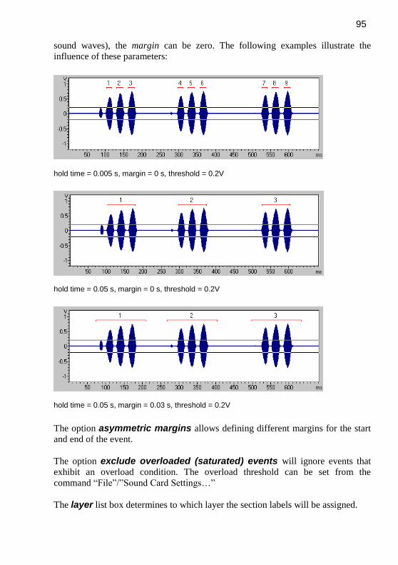
95

sound waves), the margin can be zero. The following examples illustrate the

influence of these parameters:

hold time = 0.005 s, margin = 0 s, threshold = 0.2V

hold time = 0.05 s, margin = 0 s, threshold = 0.2V

hold time = 0.05 s, margin = 0.03 s, threshold = 0.2V

The option asymmetric margins allows defining different margins for the start

and end of the event.

The option exclude overloaded (saturated) events will ignore events that

exhibit an overload condition. The overload threshold can be set from the

command “File”/”Sound Card Settings…”

The layer list box determines to which layer the section labels will be assigned.

96

If the label offset # option is activated, the starting number that will be assigned

to the first detected event can be entered. Otherwise, the first detected element will

receive the number “1”.

If the delete all previous labels option is activated, then all labels that already

exist will be deleted. Otherwise, the labels will be added to the existing ones.

The take channel # list box selects the channel from which the events are

detected.

Create labels from UltraSoundGate DI The UltraSoundGate hardware provides a digital input channel, which is located in

the least bit (bit 0) of the 16-bit PCM word. This command allows creating labels

derived from that digital input channel. The signal fed into the digital input is

assumed to be active-low.

Label placement : It can be selected one of the following locations: start of pulse : The label is placed at the start of the pulse (falling edge of the

low-active signal).

end of pulse : The label is placed at the end of the pulse (rising edge of the low-

active signal).

section : A section label representing the entire low-active pulse is created. section inverted : A section label representing the entire high-active pulse is

created.

pulse interval > In case the digital signal represents the state of a mechanic

switch, this time parameter can prevent recognizing faulty pulses (mechanic

switches sometimes produce several close-spaced pulses when being pressed). If

this is not a problem, this parameter can be set to zero. Otherwise, this parameter

should be set to a value that is smaller than the expected pulse rate (for manual

switches 10 ms would be appropriate).

Label text string : The specified string is assigned to the text label.

index : The index of the label (starting with one) is appended.

duration : The duration (for sections) or time stamp of the label is used as label

text.

delete all previous labels : If this option is activated, all existing labels will be

deleted.

take channel# : In multi-channel files, this list-box allows to select the channel

from which the digital signal is taken.

97

Create sidecar .txt file instead of labels : If activated, this option will instead

save the results in a separate .txt file.

Georeference labels / .wav files This command looks up the geographic coordinates of the labels that have been

added to a sound file that was recorded by the Avisoft-RECORDER software. In

field survey applications, it is for instance possible to display the identified species

on a map.

If there are no labels stored in the .wav file, the program can instead use different

identifiers that apply to the entire .wav file. The available options can be selected

from the list box titled “if there are no labels use xxx as identifier”:

filname prefix: The program searches for filename prefixes (separated by space

or underline characters such as ‘Ppip T0001.wav’) that have been created for

instance by using the command File/Rename and will use these strings as species

references.

dXML field: A specific dXML data field (for instance “species”) is being used as

an identifier for the waypoints to be created. The corresponding name of the dXML

field must then be entered.

Fixed string: A fixed user-defined string is being used as identifier for the

waypoints.

This option can be used for batch processing of (short) stationary files.

The GPS time stamp information that is saved in the recorded .wav files is used to

look up the geographic coordinates from a .gpx or NMEA tracklog file (note that

.kml tracklog files no not work because they do not contain the required time

stamps). Alternatively, the UTC start time of the sound file can be entered

manually. The results containing the label name, the associated coordinates and the

time stamp can be saved into a .gpx, .kml, .shp or .txt file.

Input GPS Waypoint / Tracklog File (.gpx, .kml, tcx or NMEA .txt) Select here the tracklog file from which the time stamps and GPS coordinates

should be taken. Supported file formats are the GPS exchange format (.gpx),

Google Earth (.kml with MultiTrack entries), Gamin Trainings Center (.tcx) and

NMEA 0183 formatted text log files (.txt). This would be normally the continuous

tracklog file created by the RECORDER software (Options / GPS Settings… >

‘continuous tracklog while monitoring’).

98

individual .gpx file for each .wav file (or no tracklog file) If the RECORDER software was configured to create individual log files for each

.wav file and the ‘.wav file tracklog’ option was activated, it is possible to use the

tracklog information from these individual files by activating this option.

Stationary sound files (that were recorded at a fixed place) do not require a

separate tracklog file because the fixed GPS coordinates will be taken directly from

the .wav file header (activate the option individual .gpx file for each .wav file (or

no tracklog file) in this case).

.wav file UTC start time This edit field should display the UTC start time that is stored in the file header of

the .wav file. This information is saved by the RECORDER software, version 3.4,

dated 14 January 2009 or later. If the UTC start time stamp is not available, it is

also possible to enter that time manually (format: ‘yyyy-mm-ddThh:mm:ssZ’).

Output Waypoint File Enter here the destination .gpx, .kml, .shp or .txt file name into which the results

should be written. The .gpx, .kml and .shp format options comply with the industry

standard and can be viewed in various GIS applications. The .txt format is a simple

TAB-delimited ASCII table that contains the label names, the time stamps and the

geographic coordinates.

This command can also be executed on several sound files at once by using the

associated batch command option (Tools/Batch processing…).

export the full pathname of the .wav files If this option is activated, the complete local pathnames of the .wav files will be

added to the resulting output file (only available with .kml files).

add HTML links pointing to the .wav files This edit field allows to replace the original (local) pathname of the .wav files in

the resulting .kml file by a user-defined URL, which can simplify publishing

results on Google Maps for instance. Note that the pathnames could also be

replaced afterwards in a word processor application.

launch GIS application If activated, the program will run the specified GIS (Geographic Information

System) application with the resulting .gpx/.kml file as a command line argument.

One possible program would be GoogleEarth, which can (in the current version

5.1) however only open .kml files as a command line argument. .gpx files must be

instead opened separately.

Delete all labels This command will delete all labels.

99

Filter labels The Filter labels command allows removing labels based on their label text strings.

There are generally to ways for selecting the labels to be removed which can be

selected from the combo box at the top of the dialog box::

keep the selected labels : This option will keep the labels that have been

selected on the list box below.

remove the selected labels : This option will delete the labels that have been

selected on the list box below.

Click at OK to execute the removal of the labels. In order to be able to undo the

filter operation, the wav file should be saved before this command is executed.

(Re-)Number labels Sorts the labels by time and replaces the label text by a running number.

Label settings... See page 162.

Import section labels from .txt file… Imports section labels from a common .txt file. The expected format of the .txt file

is as follows:

Start [s] end [s] optional label text

-------------------------------------------------------------------------------------- 43.2364 43.2473

63.1097 3.1193 section a

65.02916 5.0387

--------------------------------------------------------------------------------------

Import time-frequency labels from .txt file… Imports time-frequency labels from a common .txt file. The expected format of the

.txt file is as follows:

Time [s] frequency [Hz] optional label text 43.2364 4000

63.1097 5000 start

65.0291 6000

----------------------------------------------------

100

Export labels into .txt file… Exports (section) labels into a common .txt file. The format of the resulting .txt file

is compatible with the above commands Import section labels from .txt file… and

Import time-frequency labels from .txt file…

Label statistics… See page 164.

Export label data

There are two export Format options:

binary time series This option exports the labels as ASCII-formatted binary time series either via the

clipboard (Copy button) or as a text file (Save… button). The temporal resolution

of the time series can be specified in the corresponding edit field. The resulting

sample frequency is displayed below. The labeled sections are represented as “1”.

The remaining segments between them are “0”. CR/LF characters separate the

subsequent binary samples.

time / frequency stamps The time and frequency stamps of the labels will be exported as an ASCII table.

The individual label coordinates are separated by tabulators.

Insert CR/LF : In order to separate related measurements (belonging to a syllable

or song), it is possible to insert new line control characters (CR/LF) depending on

the selected option:

if label text equal to ‘.’ If there is a dot (period) in a label text, a CR/LF will be inserted and the next label

will be on the next row. In this way it is possible to group subsequent labels (e.g.

for exporting frequency contours of subsequent sound elements). The spectrogram

window command Tools/Automatic Parameter measurements/Copy peak

frequencies into labels will create the dot delimiters for the last sample of each

element automatically.

after each label A new line will be inserted after each label.

if label text is not empty A new line will be inserted if there is any label text

101

if interval > threshold A new line will be inserted if the time interval between the current and the

preceding label is larger than the specified threshold.

Add label text If activated, the label text string will be exported as well.

Save labeled sections into numbered .wav files This command saves each of the currently selected label sections of the sound file

into separate numbered .wav files. The destination folder for the files to be saved

can be entered either directly into the Destination directory field or via the Select

Directory button.(…). The option “Add the filename of the original .wav file”

will include the filename of the original .wav file as a filename prefix for the

numbered .wav file output. Use the option “Add the label texts to the filenames” in order to retain the label text information. The option “Reject file numbers” will exclude the default running number from the filename. If you use

that option make sure that the all label texts are unique (otherwise, files will be

overwritten). The “Digits” list box determines the number of digits used for

formatting the file number. Make sure that there are sufficient digits for covering

the maximum number of labels. The “Margin” value specifies the margin that is

added at both start and end of each section label.

Save labeled sections into a single .wav file…

This command saves the concatenation of the selected sections of the sound file

(selected by section labels) as a new (single) .wav file.

Save labeled sections of same class into single .wav files…

This command saves the concatenation of the selected sections of the sound file

(selected by section labels) as a new (single) .wav files. Each label class (defined

by the label text) will be saved into a separate file. In case the destination files

already exist, the new data will be appended to the existing ones.

Classify labeled sections

Labeled elements can be classified either by means of a spectrogram cross-

correlation procedure (option Spectrogram Templates) or by means of a

102

frequency contour comparison that employs a least mean square criterion (option

Frequency Contour Templates).

Spectrogram Templates

This classification option allows identifying syllables by using spectrogram cross-

correlation. A user-defined set of template spectrograms is compared with each of

the labeled sections in a soundfile (the sound event labeling can be done either

manually or automatically (see page 94). The comparison is done by a two-

dimensional spectrogram cross-correlation. The name of the template spectrogram

that provides the maximum correlation coefficient (the highest degree of similarity)

is considered as the class membership of the unknown syllable. An additional

threshold comparison on the cross correlation coefficient allows to increase the

reliability of the results. If none of the template spectrograms provides a

correlation coefficient that is larger than that user-defined threshold, the sound

event will be labeled as unidentified.

The template spectrograms that have previously been saved from the spectrogram

window command “File”/”Save Spectrogram (ASCII/Binary)…” as .son files can

be selected from the Select button or simply by drag-and-drop. The launched File

Open dialog allows to select several files at once (by using the <Shift> or <Crtl>

keys). All template spectrograms must reside in the same folder. The templates

must have been created with corresponding spectrogram parameters (same FFT

length, frame size, overlap, samplerate). Also, the sample rate of the sound file to

be examined must correspond to the sample rate at which the template

spectrograms have been created. If the option use all template files in the selected folder is activated, all the .son files in the selected folder will be used as

templates.

In order to reject low-frequency noise that might disturb the correlation procedure,

a high-pass cutoff frequency can be specified. All spectrogram components

below that frequency will be ignored. Accordingly, the low-pass cutoff frequency setting will exclude any signal components above the specified

frequency.

For tolerating slight frequency deviations between the templates and the unknown

sounds, a max frequency deviation can be specified. Depending on the

frequency resolution of the template spectrograms and the specified maximum

deviation, the cross-correlation will be repeated for various frequency shifts. The

maximum correlation coefficient is taken as the similarity score. The cross-

correlation algorithm is similar to that of the Avisoft-CORRELATOR application

(see page 235).

103

The identification threshold determines the rejection of poor identification

results. This threshold is applied directly to the cross-correlation coefficients. Any

sound event that only provides coefficients below that threshold will be regarded as

unidentified (“?”). Higher thresholds will provide more reliable classification

results. However, slight deviations between the template and the sound under

question might also prevent the proper recognition of class memberships. Adding

more templates that cover as much variations as possible can compensate this

problem. In order to get unified class names for all variations, the filenames of the

spectrogram templates (.son) that should belong to the same class must start with

identical names. The unified class names must be separated from the rest of the

filename by either a dot (.) or an underscore (_). The following set of templates

would create two classes only (e1 and e2). e1_v1 and e1_v2 represent variations

that refer to the same class.

e1_v1.son

e1_v2.son

e2_v1.son

e2_v2.con

The option create automatic classes will perform a cluster analysis in such a

way that new templates are being created automatically each time the identification

threshold is not exceeded with the current set of templates. In this mode of

operation, it is not required (but it is still possible) to define template files

manually because they can all be created automatically. The template files will

then be saved by default into the Avisoft Bioacoustics documents folder or

alternatively into the manually specified folder (simply drag the desired folder into

the Classification Settings dialog box). The button Delete old c*.son files will

delete any automatically created .son template files that are present in the current

template folder.

The results of the classification procedure can be assigned directly to the

underlying section labels. The option replace label texts with class names is

responsible for these assignments. The section labels of unidentified (?) elements

can be removed by activating the option remove unidentified sections. The

option keep text of unidentified labels will preserve the original label text in

case it could not be identified (otherwise the label will receive the ‘?’ character).

The option ignore labels with text string (except ‘?’ and numbers) will

exclude those labeled sections that already have a text string with at least one letter

in it (only labels with text strings such as ‘?’, ’1’ or ‘189’ will be processed and

labels with strings such as ‘e1’ or ‘species a’ will be excluded from the

classification procedure.

104

Due to the frame-based generation of the spectrograms, there will be (depending

on the selected FFT length) short missing intervals at the beginning and end of

each label. This effect can be compensated by activating the option compensate for FFT window size, which will extend the boundaries of the created

spectrogram (by shifting the start and end positions appropriately). The related

zero padding option will set these margins (FFT length / 2) to zero in order to

prevent potential overlapping with adjacent sounds.

In case multiple templates have been defined for each class, the option classify based on averaged correlation values will perform the classification based

on the maximum average correlation coefficient of all templates belonging to each

class.

The option max duration difference between template and section label allows to limit the template comparison to templates having a duration similar to

the duration of the section label to be examined. This can help prevent miss-

classifications due to high correlation values between long complex sound

elements that would otherwise produce high correlation values when compared to

short and less complex templates. The maximum duration difference threshold

[unit ms] should be selected according to the typical durations. In order to make it

work, it is necessary that the total duration of each template spectrogram reflects

the duration of the sound element in it (there should be uniform margins) and that

the section labels to be examined exhibit margins similar to those in the templates.

The section label layer list box determines which labels will be used for the

classification procedure.

Frequency Contour Templates

This classification method compares the frequency contours of the labeled sections

with template frequency contours. The similarity between the labeled sections and

the templates is determined by calculating least mean squares. The frequency

contour templates are defined by .ft files that can be created by the Graphic

Synthesizer module (the command File/Save As… saves .ft files that are part of

an arrangement (.ARR)). The frequency contours itself can be created either

manually in the Graphic Synthesizer by mouse-drawing or they can be derived

from spectrograms (spectrogram window command Tools/Scan frequency contour an and amplitude envelope…). The frequency contours of the labeled

sections are determined by searching the peak frequencies on the spectrogram,

which means that this kind of classification will only work for whistle-like

vocalizations that exhibit clear frequency contours. The advantages of this method

are that the calculation of the similarity score is fast and that the time scale can be

varied by applying the time warping option.

105

The final classification is done by calculating the root mean square of the

frequency differences between the two contours. This means that the marked

section receives the class name of the template that provides the minimum overall

frequency deviation. In case the durations of the template and the detected call

differ by more than a predefined percentage (as specified in the +- xxx % field on

the section titled “duration”), then this detected call will be skipped. The option

“normalize duration” aligns the time scales of the templates before the

similarity score is calculated. The option “time warping” will repeat the

correlation at different time scales.

The option Filter Classification Results allows to pick out a single class out of

the classified labels (by deleting all section labels that have been assigned to other

classes). The take class list box selects the desired class. The option replace label texts with index will assign the running index to the filtered labels. The

labeled sections that

The Default button will set all parameters to their default settings.

The classification procedure is initiated by clicking at the Start button. A new

classification window will appear:

Classification Report

The Classification Report panel indicates the progress and the results of the

classification procedure. The report table lists the calculated correlation

coefficients, the assigned class names and time stamps of each section label. The

running classification can be prematurely canceled by clicking at the Cancel button.

Revise thresholds (only available on the command “Scan for template

spectrogram patterns”) allows to repeat the final classification with a modified

identification threshold and masking interval without executing the time-

consuming cross correlation procedure again.

Show CCF traces (only available on the command “Scan for template

spectrogram patterns”) displays the cross-correlation traces of the template

comparisons.

106

The class / cnt table lists the total number of events that have been assigned to

each class. The buttons Save stat and Copy stat export the class / cnt

information.

The buttons Save table and Copy table export the detailed classification report

table.

Use the batch command (Tools/Batch processing…) for processing several sound

files at once.

Detect and Classify waveform events This command combines the two commands Create section labels from waveform events (see page 94) and Classify labeled sections (see page 101).

Classify Element Sequences

The Element Sequence Classifier facilitates identifying user-defined label

(element) patterns. The list box at the top of the dialog box represents the defined

sequence classes. Each sequence class is identified by its class name. The label

sequence is defined by enumerating the individual label texts (separated by space

characters) in the sequence field.

class name : Enter here the name of the class.

delete : Removes the selected class.

new : Adds a new class.

107

< : Moves to the previous class.

> : Moves to the next class.

sequence : Enter here the label texts in the desired order. The individual labels

must be separated by space characters.

It is possible to insert optional interval and/or break limits between the labels that

override the corresponding limits defined in the general settings section. The

optional temporal limits must be separated by space characters and must have the

following format:

i>ddd.dd

i<ddd.dd

b>ddd.dd

b<ddd.dd

The unit of the duration parameter ddd.dd is milliseconds.

For example the sequence string “class1 b>100 b<200 class2

class3” defines a sequence of 3 elements class1, class2 and class3. The

duration of the break between class1 and class2 should be larger than 100 ms and

shorter than 200ms. The break between class2 and class3 is as defined on the

general settings > break between elements.

loop : The loop option defines a sequence that repeats itself several times.

Reset : Removes all class definitions and returns to the default class definition file

seq_classes.scs.

.

general settings : The general setting section defines additional constraints on

the defined class by limiting the range of a number of parameters. Leaving the

corresponding edit fields empty will ignore the parameter.

element interval : The duration from the start of the previous label to the start of

the current label. These interval limits can be overridden by the i>ddd.dd and

i<ddd.dd options as described above.

break between elements : The duration from the end of the previous label to

the start of the current label. Use the upper limit of this parameter in order to

separate consecutive groups of elements (strophes). These break limits can be

overridden by the b>ddd.dd and b<ddd.dd options as described above.

108

total number of elements : The total number of labels in the entire sequence.

These limits only apply if the loop option has been activated.

total group duration : The duration from the start of the first label to the end of

the last label of the sequence.

average element rate : The number of elements per seconds on the entire

sequence.

copy! : Copies the settings from the currently selected class to all other classes.

default! : Resets the select class settings and sets the maximum break between elements to 500 ms in order to separate consecutive strophes.

reset! : Resets the select class settings.

delete the original labels : If activated, the original labels (single point labels or

section labels on layer 1) will be deleted. It is recommended to disable this option

while optimizing the settings.

Start / OK : Clicking at the Start button will execute the classification procedure.

The identified sequences will be marked by section labels on layer 2 (or layer 1 in

case the above option “delete the original labels” is activated) and will be

enumerated in the listbox at the bottom of the dialog box.

Cancel / Close : Terminates the dialog box.

SaveAs… : Saves the element sequence class definition in a new .scs

configuration file.

Open… : Opens a previously saved .scs file. Alternatively, existing .scs files can

be opened by drag&drop.

This command can be executed also in a batch process (Tools / Batch processing… > Classify Element Sequences).

Section label grid... See page 162.

DDE parameters / Log-file... See page 139.

Touch Screen Optimizations

This dialog box allows adjusting a number of settings that improve the operation of

the graphic interface of the software on a touch screen. Note that this dialog box

can also be launched on the SASLab start screen with the Avisoft logo by left-

clicking (or touching) the area with the frame.

109

apply these settings If activated, the following settings will be applied. Otherwise, the graphic interface

will work in the conventional mode for mouse-based control. Use this option to

quickly switch between touch and mouse control.

button size : Selects the desired enlargement of the buttons.

snap distance : Selects the snap distance for managing cursors

push scrolling : Enables the push scrolling mode that continues scrolling after

releasing the touch screen (or mouse button) depending on the speed of the push

movement and the selected friction setting. A friction setting of 0 will scroll

endlessly until the end of the file is reached or the user stops the scrolling by

touching or left-clicking at the display. Higher friction values will continuously

slow down the speed down to zero. The update rate determines how often the

display is being updated. High rates (25 fps) will provide a smoother scrolling but

at the same time create a higher processor load.

scroll mode : Activates the scroll mode at which the entire waveform and

spectrogram display area can be used to scroll (pan) through the sound file.

Otherwise, that area will be sensitive to inserting markers and moving cursors.

display large scroll mode / control buttons : Launches large buttons for

controlling the touch screen functionality (scroll mode and optionally the shift and

right-click emulation).

emulate shift key / right-click : Displays buttons for emulating the shift key

and right-click mouse control functionality on the SASLab software when the

Scroll Mode is not activated:

The Shift Key button represents the shift key on the keyboard, which allows

inserting labels that would normally require to press the shift key on the keyboard.

The Right-Click option will translate a left-click (a touch) into a right-click in

oder to facilitate entering label texts for instance.

auto reset : The auto reset option determines the behavior of the shift key and

right-click emulation. If activated, both the shift key and right-click buttons will be

deactivated once an action has been executed. That way, the shift key and right-

click emulation will only be applied temporarily for the next touch. Otherweise,

these options will remain active until the corresponding keys are deactivated

manually.

110

previous/next file command functionality : If activated, the scroll mode will

move to the previous or next file (according to the settings defined

File>Specials>Previous/Next file command settings…) once (in a zoomed view)

either the start or the end of the WAB file has been reached and the user tries to

move further. If the entire file is being displayed, the command will be executed

once the touch screen is released near the margins of the program window (similar

to the common tablet gesture).

When using the software on a tablet PC with touch screen (without a stylus) it is

generally recommend to enlarge the text and the items from the Windows Control

Panel > Display. Similarly, the file icons on the Explorer window and File Open

dialog box should also be enlarged (“Medium” or “Large Icons”).

Calibration

The Calibration dialog box allows calibrating a sound file or the recording

equipment for absolute or voltage level or sound level measurements.

The calibration is basically achieved by determining the absolute measurement

range (full-scale range) of the recording equipment at a certain gain setting. The

full-scale range is defined as the maximum level of a sine wave that can be

recorded without clipping.

In case the absolute full-scale range is

already known, it can be entered directly

into the corresponding edit field and no

further action would be required. If this

is not the case, the measurement range

must be determined by recording a

reference signal whose absolute level is

known.

Depending on the available information

on the full-scale range and the

microphone (or hydrophone) sensitivity

and the purpose of the measurements,

one can select the desired calibration

method from the Method list box at the

top of the dialog box. The following

options are available:

111

No calibration (re 0 dB FS) This option represents the uncalibrated state, where all measurements within in the

SASLab Pro software are referenced to a default voltage level of 1V on linear

measurement scales and 0 dBFS on logarithmic measurement scales. This means

that all dB measurements will be negative values. A full-scale sine signal

corresponds to a level of -3dBFS and a full-scale square signal would correspond

to a level of 0 dBFS. This is the default setting for applications that do not require

absolute sound level measurements.

Voltage level measurements This option is intended for absolute voltage level measurements. The full-scale

range can be entered in various units that can be selected from the associated list

box (see below). The gain field allows to specify any additional gain of the

recording equipment. The effective range including the specified gain is displayed

behind the gain selection field. If the full-scale range is unknown, it can be

determined by recording a reference signal whose voltage level is known (see

section Reference Signal).

SPL with calibrated phone This option is intended for absolute sound pressure level (SPL) measurements,

where the sensitivity of the microphone (mV/Pa) or hydrophone (dB re 1V/µPa) is

known. In order to determine the full-scale SPL, it is required to know the full-

scale input voltage range of the recording equipment, which can be entered in

various units that can be selected from the associated list box (see below). The gain

field allows to specify any additional gain of the recording equipment. The

effective range including the specified gain is displayed behind the gain selection

field. If the full-scale range is unknown, it can be determined by recording a

reference signal whose voltage level is known (see section Reference Signal). SPL measurements require to select the correct reference SPL, which is 20 µPa

for measurements in air and 1 µPa in water.

The microphone sensitivity is expected in mV/Pa and the hydrophone sensitivity must be entered in dB re 1V/µPa.

The full-scale SPL that results from the entered full-scale input voltage range, gain

and phone sensitivity will be displayed at the bottom of the dialog box.

SPL with reference sound This option is intended for sound pressure level (SPL) measurements were a

known reference sound source is available or where the full-scale range of the

recording equipment [expressed in Pa or dB(SPL)] is already known. The gain

field allows to specify any additional gain of the recording equipment. The

effective range including the specified gain is displayed behind the gain selection

field. If the full-scale SPL range is unknown, it can be determined by selecting a

reference signal whose sound pressure level is known. For doing this, the recorded

112

reference signal must be selected on the SASLab Pro main window by using the

marker cursor (see also section Reference Signal).

full-scale range The full-scale range corresponds to the voltage or sound pressure level that just

does not cause clipping on the sound file. It is also referred to as measurement

range.

/ gain [dB] The gain field allows to specify additional gain settings that have been selected on

the recording hardware.

Voltage level measurement units Absolute voltages can be specified in various units:

Vp : peak voltage

Vpp : peak-to-peak voltage

Vrms : root mean square voltage

dBV : logarithmic expression of the above root mean square voltage, referenced to

a voltage level of 1Vrms.

dBu : logarithmic expression of the root mean square voltage, referenced to a rms

voltage level of 0.775 Vrms.

For a sine wave signal, the different units can be converted as follows:

1 Vrms = 1.414 Vp = 2.828 Vpp = 0 dBV = 2.2 dBu

In multichannel files, it is possible to calibrate each channel individually by

selecting the individual channels from the channel # list box and specifying the

associated full-scale ranges. If it is not required to calibrate each channel separately

(in case all channels were uniform), the calibration executed on one channel can be

automatically transferred to all other channels by activating the option “Apply the calibration of this channel to all other channels”.

If the “option apply the calibration of this channel to all other channels” is activated, the specified calibration will be applied to all channels of

the sound file. Otherwise, the individual channels can be calibrated individually.

Reference Signal This section allows to determine the full-scale range based on a reference signal

that has already been recorded into a sound file. To execute this kind of calibration,

the previously recorded reference signal must be selected on the SASLab Pro main

113

window by using the marker cursor and the level of that signal must be specified in

the level field.

The calibration method “SPL with reference sound” allows to specify the SPL

of the reference signal either in Pa or dB(SPL). The SPL is usually being measured

by the “root mean square” (rms) method. For special applications, the option

“allow peak level measurements” will allow to select also the peak or peak-to-

peak amplitude methods for that.

The other calibration methods require to enter a reference voltage level. The

measurement method for this reference voltage can be one of the following: peak (Vp), peak-to-peak (Vpp) or root mean square (rms). The rms option allows

to specify the rms voltage level either in Vrms, dBV or dBu units. After specifying

the reference signal and selecting the reference signal within the sound file, the

Calibrate! button must be clicked in order to finally calculate the full-scale range

based on the entered reference level and the relative marked reference signal in the

.wav file. As a result, the full-scale range at the top of the dialog box will be

updated. Note that the Calibrate! button will always reset the gain setting to 0dB.

The button Calibrate all channels! will perform the calibration procedure

(individually) for all channels at once. This requires however that the reference

signal has been recorded simultaneously onto all channels (the marked section

must on all channels contain the reference signal).

Update! The Update button can be used to update the full-scale range and SPL displays

after the gain or microphone/hydrophone sensitivity has been modified.

114

Batch processing

Batch processing allows executing a function on several sound-files at once. The

following functions are available:

Print multiple line spectrogram A spectrogram is generated and printed as a multiple line image.

Print single line spectrogram A spectrogram is generated and printed as a single line image.

Save multiple line spectrogram A spectrogram is generated and saved as a multiple line image. The filenames of

the graphics files will be derived from the names of the sound files. The extension

.WAV will be replaced by .WMF, .TIF and .BMP.

Save single line spectrogram A spectrogram is generated and saved as a single line image. The filenames of the

graphics files will be derived from the names of the sound files. The extension

.WAV will be replaced by .WMF, .TIF and .BMP.

IIR-filter Each sound file will be filtered using the parameters defined in the menu

Edit”/”Filter”/” Time domain IIR filter”. The original sound files will be replaced

by the output of the filtering process.

FIR-filter Each sound file will be filtered using the parameters defined in the menu

”Edit”/”Filter”/”Time domain FIR filter”. The original sound files will be replaced

by the output of the filtering process.

Frequency Domain Transformation Each sound file will be filtered using the parameters defined in the menu

”Edit”/”Filter”/” Frequency Domain Transformation…”. The original sound files

will be replaced by the output of the filtering process.

Save one-dimensional transformation (WMF) The function selected in the menu ”Analyze”/”One-dimensional transformation”

will be executed on the sound files. The results will be saved as a WMF-graphics

file. The filenames of the graphics files will be derived from the names of the

sound files. The extension .WAV will be replaced by .WMF.

115

Save one-dimensional transformation (ASCII) The function selected in the menu ”Analyze”/”One-dimensional transformation”

will be executed on the sound files. The results will be saved into separate ASCII

files The filenames of the ASCII files will be derived from the names of the sound

files. The extension .WAV will be replaced by .TXT.

Save one-dimensional transformations into a single ASCII file The function selected in the menu ”Analyze”/”One-dimensional transformation”

will be executed on the selected sound files and the data will be saved in a single

ASCII file. In case one of the spectral functions has been selected and the Spectral

Characteristics tool is activated, then these spectral characteristics measurements

will be saved rather than the underlying spectral data set.

The resulting text file will be saved into the same directory as the selected sound

files and it’s filename will be derived from the name of the selected one-

dimensional transformation (e.g. “Envelope.txt”). If the option “Tools” /

”DDEParameters / LOG file” : “Enable Dynamic Data Exchange” has been

activated and an Excel worksheet is open, the results will also be transferred into

that Excel worksheet.

Save mean spectra into a single ASCII file A spectrogram will be calculated by using the parameters selected from

“Analyze”/”Spectrogram Parameters…” and the mean spectrum of the entire

spectrogram (sound file) will be saved into a single ASCII file. This file will be

saved into the same directory as the selected sound files and it’s filename will be

“mean spectra.txt”. If the option “Tools” / ”DDE Parameters / LOG-file” :

“Enable Dynamic Data Exchange” has been activated and an Excel worksheet is

open, the results will also be transferred into that Excel worksheet.

Save ASCII/Binary spectrogram A spectrogram is generated and saved as ASCII or binary file. The filenames of the

files will be derived from the names of the sound files. The extension .WAV will

be replaced by .TXT or .SON.

Sampling Frequency Conversion Each sound file will be converted using the settings made in the command

”Edit”/”Format”/”Sampling Frequency Conversion...”. The source sound files will

be replaced by the output this process.

Restore the original time scale of time-expanded recordings Each sound file will be converted using the settings made in the command

”Edit”/”Format”/”Restore the original time scale of a time-expanded recording…”.

The source sound files will be replaced by the output this process.

116

8<-->16 Bit Conversion Each sound file will be converted from 8 to 16 if the source file is 8 bit. 16-bit files

will be converted to 8 bits. The source sound files will be replaced by the output

this process.

Stereo->Mono Each sound file will be converted into a mono file. The conversion will be done

according to the settings made in the corresponding command Edit/Format/Stereo-

>Mono. The source sound files will be replaced by the output this process.

Automatic parameter measurements A spectrogram is generated from each sound file and the measurements defined in

the spectrogram window menu “Tools”/”Automatic parameter measurements

setup...” will be made. The results will be saved in a LOG file or will be transferred

by DDE as specified on the menu item “File”/”DDE Parameters / Log file...”.

Automatic parameter measurements; save elements as labels Same as above, except that the detected elements will also be saved as section

labels into the original .wav files.

Automatic parameter measurements; remove gaps A spectrogram is generated from each sound file and the element separation of the Automated Parameter Measurements tool is carried out. The gaps between the detected elements will then be removed from the wav file (similar to the APM window command Export/Remove gaps between detected elements from sound file…).

Sound file format conversion The selected sound files will be saved in the format specified in the ”File”/”Save

As” dialog box. The original files will not be overwritten or deleted

Change Volume The selected sound files will be modified according to the current settings in the

“Edit”/”Change Volume..” dialog box. The original files will be replaced by their

modified versions.

Shred into numbered .wav files The selected sound files will be shredded into numbered .wav files according to the

settings made in the “File”/”Specials”/”Shred into numbered .wav files…”. The

original .wav files will remain unaffected.

117

Remove silent sections The silent sections within the selected sound files will be removed according to the

settings made under “Edit”/”Compress”/”Settings”. The original files will be

replaced by their compressed versions.

Save events into numbered .wav files The sound events within the selected sound files will be copied into numbered

.wav files. The (threshold-based) event detection is executed according to the

settings made under “Edit”/”Compress”/”Settings”. The original .wav files will

remain unaffected.

Save labeled sections into numbered .wav files The labeled sections of the selected sound files will be copied into numbered .wav

files. The margin parameter specified under Tools/Labels/’Save labeled sections

into numbered .wav files…’ will be used. The original .wav files will remain

unaffected.

Pulse Train Analysis A Pulse Train Analysis is performed for each file (according to the settings made

in Analysis/Pulse Train Analysis). The detected pulses and pulse groups will be

saved into ASCII files. The ASCII file names are a combination of the original

sound file name and the strings _pulses.txt and _groups.txt.

Split multichannel files into mono files (into the same folder) The selected multichannel files (sound files containing more than one channel) will

be split into mono files. The original multichannel files will remain unaffected. The

file names of the newly created mono files will consist of the name of the original

file and the channel number (filename.wav filename_0.wav ;

filename_1.wav; filename_2.wav; …)

Split multichannel files into mono files (into separate folder) The selected multichannel files (sound files containing more than one channel) will

be split into mono files. The original multichannel files will remain unaffected. The

resulting mono files will be saved into the newly created folders channel1,

channel2, channel3… The filenames of the created mono files will be identical to

the names of the original multichannel files.

Classify labeled sections The labeled sections of the selected sound files will be classified according to the

settings made in “Tools”/”Labels”/”Classify labeled sections…”. Additionally, the

classification report table will be saved as an ASCII file (filename.txt). The

118

ASCII file filename_stat.txt reports the number of events that have been

assigned to each class.

Classify .wav or .son files (show results in a single table) The selected .wav or .son files will be classified (by using a spectrogram image

cross correlation technique) according to the settings made in the Classification

Settings dialog box that will be launched after clicking at the Start button on the

Batch processing dialog box. The classification results can be exported by means

of the Copy table or Save table buttons on the Classification Report window.

Detect and classify sound events The sound events in the selected sound files will be detected and classified

according to the settings made in “Analyze/Specials/Detect and classify waveform

events…”. The classification report table will be saved as an ASCII file

(filename.txt). The ASCII file filename_stat.txt reports the number

of events that have been assigned to each class.

Detect, classify and save sound events This command is similar to the above command Detect and classify sound events,

except that it will additionally save the detected events into numbered .wav files.

This command might be used for scanning large numbers of long sound files for

certain vocalizations.

Scan for template spectrogram patterns and save This command is similar to the above command Scan for template spectrogram

patterns, except that it will additionally save the detected events into numbered

.wav files. This command might be used for scanning large numbers of long sound

files for certain vocalizations.

Template Cross Correlation on short files This command is similar to the above command Scan for template spectrogram

patterns, except that it is prepared for classifying short .wav or .son files containing

only a single call. That way, the maximum cross-correlation coefficient across the

entire .wav file is being determined against each template file and listed in a

compact results table.

119

Noise reduction filter The selected sound files will be noise-filtered according to the settings made in the

command Edit/Filter/Noise Reduction… The original sound files will be replaced

by output of the noise gate filter.

Georeference labels / .wav files The labels (or filename prefixes) of the selected files will be georeferenced

according to the settings made in the command Tools/Labels/Georeference

labels… The results will be written into a single .gpx, .kml, .shp or .txt file.

Sort files using APM classes The selected sound files will be sorted into class-specific subfolders that are

determined by using the classification option of the Automatic Parameter

Measurements tool.

Sort files using template spectrograms (triggered CCF) The selected sound files will be sorted into class-specific subfolders that are

determined by using the command ‘Analyze’/’Specials’/’Detect and classify

waveform events…’

Sort files using template spectrograms (continuous CCF) The selected sound files will be sorted into class-specific subfolders that are

determined by using the command ‘Analyze’/’Specials’/’Scan for template

spectrogram patterns…’

Modify BWF (bext chunk) metadata Modifies the bext chunks of the selected .wav files. If there is already a bext chunk

in a file, then the new data can either be appended to the existing data (option

“append”) or it can replace the existing data (option “overwrite”).

Save application-specific (dXML chunk) metadata Saves uniform dXML records into the selected .wav files.

Create virtual Metadatabase Collects various metadata items of the selected .wav files into a XML-formatted

metabase.

Insert silent margins Silent sections of the specified duration will be inserted at the start and the end of

each file.

120

Scan frequency contour and amplitude envelope Scans the frequency contour and amplitude envelope as setup in the corresponding

spectrogram window command on the Tools menu and saves the resulting .at and

.ft files.

Create envelope (*.env) sidecar files Creates .env sidecar files according to the selected Overview Display Parameters

and the envelope resolution (FFT frames) setting on the command File/File Open

Settings…

Create section labels from waveform events Executes the command Tools/Labels/Create section labels from waveform

events… in a batch process.

Insert USG DIO Time Code / Pulse Train / Single Pulse Executes the command “File”/”Specials”/”UltraSoundGate DIO”/”Insert time code

/ pulse train / single pulse…” in a batch process.

Classify Element Sequences Executes the command “”Tools/Labels/Classify Element Sequences… in a batch

process.

All functions use the parameters and options selected in the associated dialog

boxes of the underlying commands.

process all files in the selected folder If this option is activated, the batch procedure will process all files that reside in

the selected folder and have the specified extension.

include first-level subfolders If activated, sound files that are located in first-level subfolders will also be

processed.

include all subfolders If activated, sound files that are located in the specified folder any subfolders will

be processed.

launch setup dialog boxes If activated, the setup dialog boxes for the selected function will be launched

before the batch process is started. Uncheck this option in order to bypass these

dialog boxes if you don’t need to adjust anything.

121

Files… The Files… button launches the file selection dialog box, which supports multiple

selections by using the Ctrl key. Alternatively, it is possible to drag and drop the

desired files into the Batch processing dialog box.

Folder… If the option ‘process all .wav files in the selected folder’ has been activated,

the Folder… button allows to select the desired folder. Alternatively, it is possible

to drag and drop at least one file of the desired folder into the Batch processing

dialog box.

The currently selected files will be listed in the Batch processing dialog box.

Start The Start button starts the batch process.

Once the batch process is running, the procedure can be cancelled prematurely by

clicking at the Cancel Batch Processing button.

Real-time processing The real-time processing tool allows processing newly recorded .wav files once

they have been closed by the recording software (Avisoft-RECORDER for

instance). The commands that can be executed in real-time are the same as those

available on the Batch processing tool. The software will permanently look for

new files in the specified folder. That folder cane be selected from the Folder...

button or by dragging it from the Windows Explorer window into the Real-time

processing panel.

Click at the Setup button to configure the selected command and then at Start to

finally start the real-time process. The Pause button will inhibit the real-time

processing temporarily until the Continue button is pressed. The Cancel button

will terminate the process and close the Real-time processing panel. The list on

the bottom of the window will report the processed files along with a few

benchmarks.

The real-time processing tool can be launched automatically on the SASLab Pro

program start by activating the option Actions/On program start/Launch Real-time

processing tool, making it possible to setup an unattended automated processing

system.

122

The real-time processing option “Classify short .wav or .son files (show results in a

single table)” allows generating class-specific responses by executing user-defined

batch (.bat) files. In order to make this work, it is necessary to create a .bat file for

each class that should generate a response. The filenames of the .bat files must

match the names of the classes and must reside in the same folder as the .son

template files. The .bat filename for the class “?” must be “undefined.bat”.

123

Metadata dXML database records >

This submenu allows to define and edit user-defined metadata that will be

embedded into the currently opened .wav file. At first, the database structure must

be defined from the command dXML database records > Define database

structure... The individual dXML data records of a set of .wav files can be merged

into a virtual metabase at any later time (on-the-fly). This concept makes sure that

the integrity of the metadatabase is always inherently preserved.

Edit... This command launches the dXML metadata record edit box according to the

previously defined data base structure (command Define database structure...).

The entered data will be saved along with the .wav file when the command

File/Save is executed or when the .wav file is being closed. If the option “multiple

records” has been activated on the Define database structure... command, then it is

possible to add additional records by clicking at the new button. The individual

records are then displayed in table and can be edited by navigating to the

corresponding row by using the < and > buttons or by clicking at the desired row.

The delete button will remove the selected record. Modified fields will be saved

automatically when a new record is launched or manually be clicking at the Enter

button. The Text modules menu provides predefined text modules that have been

defined from the main window command File > Rename by text module / Define text module. If the main window option File > Rename by text module / Define text module > Paste text module into the first dXML field (instead of renaming) is activated, the text modules accessed from the

main window will automatically pasted into the first dXML field.

Batch Edit... The Batch Edit command allows to save a uniform dXML data to a number of

.wav files at once. This is done by launching the corresponding Batch processing

dialog box. Select here the desired .wav files and then enter the data record(s).

Define database structure... This dialog box defines the user-defined dXML data fields. Each data field is

represented as a individual row.

field name: Each data field must be given a unique field name, which cannot

include special characters such as < or >.

124

type: A field can have one of the following data type attributes: text, bool, integer, float, date or time. The format of these data types is as follows:

text : abc123

bool : 0, 1

int : 123

float : 1.23

date: yyyy-mm-dd

time: yyyy-mm-dd hh:mm:ss

The date and time data types will automatically enumerate the current date/time

and file creation/modification date in their corresponding combo boxes.

size: Defines the maximum size of the text, integer and float types.

valid entries or pick list: When the file type text is selected, this edit field

allows to define a set of strings that are allowed to enter or that will appear as a

pick list. The individual strings must be separated by commas (“,”). A list of valid

strings (such as species names) can be imported by clicking at the imp button.

validation: If activated, only the specified list of strings will be accepted.

Otherwise, the defined list of strings will be displayed as a pick list. In case there

are no strings defined in the valid entries or pick list field and the validation

option is activated, the data base field cannot be empty (null).

imp : Imports a list of strings from a text file into the valid entries or pick list

field. The individual string the in the .txt file must be separated by CR/LF control

characters. The external .ext file can also be read by drag&drop (the cursor must be

placed into the desired field before).

lock : If activated, this option will lock the corresponding input field (it will be

grayed). Use this option to prevent unintentional modifications on the specific

field.

A new field can be inserted by clicking at the Add button and the selected filed

can be removed by the Remove button. The selected field (marked by the check

box in the row titled select) can be moved by using the up and dn buttons.

The OK button will save the defined data base structure into a separate .xml file

(whose name is displayed at the bottom of the dialog box). The Open button

allows to open one of the previously saved .xml database structure files. The

SaveAs button will save the database structure under a new filename. The Reset

button will reset all fields.

125

display show . If activated, the dXML edit field will always be launched automatically.

lock: If activated, it is not possible to edit the dXML data in order to prevent

undesired modifications. This global lock option will affect all data fields

regardless whether the individual field-specific lock options are activated or not.

multiple records : If activated, it is possible to enter more than one data record

for each .wav file.

history show: If activated, this option will memorize all entered data and it will be

possible to select these previous data from a pick list.

reset: Resets the history data.

XML View... Launches the selected XML viewer application (command Metadata> Select XML

viewer...) and displays the dXML data record(s) within that application.

Copy This command copies the current XML-formatted dXML data set into the

clipboard. It can then be pasted from the corresponding Paste command in SASLab

Pro or it can be imported into another XML application such as the Microsoft

XML Notepad.

Paste This command will paste a XML-formatted dXML data set from the clipboard.

Remove This command will completely remove the dXML chunk from the currently

opened .wav file.

mXML measurements >

This submenu provides commands for managing measurement data that are

embedded into the .wav file. This measurement logging functionality can be

activated from the command Metadata > mXML measurements > Enable mXML

data logging or from Tools > DDE Parameters, Log File… If activated, the

measurements will be saved into an application-specific RIFF chunk titled

“mXML” each time when a measurement copy command is executed. The logged

measurement data can be viewed and edited from the command Metadata >

126

mXML measurements > View entries… In addition to that, the individual mXML

datasets of a bunch of .wav files can be collected and queried from the command

Metadata > Create Metadatabase… Enable mXML data logging This option enable the mXML data logging mode. If activated, the measurement

data will be saved into the application-specific mXML RIFF chunk, each time an

copy measurement command is executed.

View entries… The mXML Overview window displays the mXML measurement data. There are

two list boxes. The list box on the top shows all mXML data records, indicating the

type of measurement data and the date, when the measurements were taken. The

other box at the bottom shows the content of the currently selected data record.

Selection Copy: Copies the selected ASCII-formatted (TAB-delimited) data record into the

clipboard.

Delete : Deletes the selected XML-formatted data record.

Copy Copies the XML-formatted mXML data into the clipboard. These data can then for

instance be pasted into the Microsoft XML Notepad.

Remove This command will completely remove the mXML RIFF chunk from the .wav file.

Save As… Saves the mXML data into a .xml file.

XML View… Launches the selected XML viewer application (command Metadata> Select XML

viewer...) and displays the mXML data record(s) within that application.

View XML RIFF chunks > Allows to view any .wav file RIFF chunk that contains the substring “XML” in its

RIFF identifier (such as “iXML” for instance).

Select XML viewer... Selects the application for the above View XML RIFF chunks command. A suited

application would be the free “XML Notepad” application by Microsoft

127

(http://www.microsoft.com/downloads/details.aspx?familyid=72d6aa49-787d-4118-ba5f-

4f30fe913628&displaylang=en), an internet browser application or Microsoft Excel.

bext (BWF) Metadata... > This menu provides tools for editing embedded (bext RIFF chunk) metadata

complying with the Broadcast Wave Format standard.

Edit This dialog box allows to view and edit the metadata information that is stored in

the ‘bext’ chunk of the Broadcast Wave Format (BWF) wave file format. If the

currently opened file does not already contain a bext chunk, this command allows

to add additional metadata information to the .wav file.

The OK button reads the modified metadata information from the dialog box, but

still does not update the underlying .wav file. The modified metadata information

can be saved from the command File/Save.

The Reset button will reset (delete) the bext metadata information. The Save file

button saves the currently opened .wav file along with the edited metadata (it

combines the OK button function with from the command File/Save).

The format of the BWF metadata fields that can be edited is as follows:

Description: 256 characters

Originator: 64 characters

Originator Ref: 32 characters

Origination Date: 10 characters, must be entered as “yyyy-mm-dd” Origination Time: 8 characters, must be entered as “hh-mm-ss” Coding Hist: Unlimited number of characters

Batch Edit The batch edit command is similar to the above Edit command, but it is applied to

a set of .wav files by using the corresponding Batch processing command option.

Create Metadatabase...

This command can collect the individual dXML, mXML and other file-specific

metadata information from the selected individual sound files into a single XML

table. This is done by using the corresponding Batch processing option.

128

When the Create Metadatabase command is executed at the first time or if the

related command Define and create virtual Metadatabase… is executed, a

dialog box titled Virtual Metabase setup is launched, which allows to select the

desired metabase data fields. In addition to that, there are a number of options for

creating sidecar files (sidecar files contain related information on the individual

.wav files. Their filename is identical to name of the original .wav file, except that

they have a different extension, such as .gpx or .xml).

Select metabase fields

filename with full path : If activated, the full pathname of the .wav file is taken.

Otherwise, only th efilename without the path will be saved.

filename prefixes : Prefixes preceding the actual filename string (separated by

space characters) will be enumerated.

sample rate : Sample rate of the sound file in Hz. bit-depth: Number of bits in each sample (usually 8, 16 or 24 bits)

number of channels duration: Duration of the soundfile in seconds

creation date: Creation date of the sound file taken from the file system of the

operating system.

modification date: Modifification date of the sound file taken from the file

system of the operating system.

bext origination date: Origination date taken from the bext RIFF chunk of a

BWF file.

RECORDER creation date: Creation date taken from the TIME chunk created

by the Avisoft-RECORDER software.

GPS coordinates: The latitude, longitude and elevation taken from the GPS

chunk created by the Avisoft-RECORDER software. The coordinates are

expressed in the WSG 84 format.

GPS UTC time stamp: The UTC date and time taken from the GPS chunk

created by the Avisoft-RECORDER software.

dXML database fields: The dXML data fields entered in the RECORDER or

SASLab Pro software.

mXML measurements: The mXML measurement data logged by the SASLab

Pro software.

number of labels: The number of labels in the sound file.

label list: Complete list of all labels in the sound file.

iXML RIFF chunk: The complete iXML RIFF chunk of a BWF file.

129

bext RIFF chunk (BWF): The bext chunk fields of a BWF file.

Create sidecar files coordinates (*.gpx) coordinates (*.kml) dXML (*_dxml.xml) mXML (*_mxml.xml) labels (*.lbl) labels (*_labels.xml) iXML RIFF chunk (*ixml.xml)

Output XML output filename (…) : Enter here the filename of the resulting matebase

.xml file or us ethe … button to select the desired path..

Create flat XML structure: If activated, a flat XML structure with a reduced

level of hierachy will be created.

Launch XML viewer application: If activated, the selected XML viewer

application will launched to display the resulting metabase .xml file.

XML viewer application (…): Select here XML viewer application. A suite

application woul dbe for instance the Microsoft XML Notepad, an internet brower

or Microsoft Excel.

The creation of the metabase can be started by clicking at the OK button.

The resulting metabase will be displayed in a table titled Metabase: Metabase expand: If activated, potential multiple entries (more than one record per file) will

be displayed.

Open file: Opens the currenty selected .wav file in the SASLab Pro main window.

browse: If activated, the currently selected file will be automatically opened in

the SASLab Pro main window.

GIS exp…: Exports selected metabase data fields into a .gpx or .kml file or the

entire metabase into a shapefile. This button is only available if there are

geographic coordinates in the metabase.

Copy: Copies the metabase table into the clipboard (as a TAB-delimited ASCII

table).

Query: Query command for filtering the metabase.

130

Folder…: Use this button to create a metabase of another folder using the

previous settings. Alternatively, the desired folder can be dragged into the

Metabase dialog box.

Update! : Updates the metabase using the previous settings.

Open xml: Opens the underlying .xml metabase file in the specified XML viewer

application.

Phenology: Generates phenology histogram data (number of .wav files on a day

versus time of day table) based on the date attribute of the .wav files in the

metadatabase.

Metabase GPX / KML / SHP Export

The Metabase GPX / KML / SHP (GIS) Export tool allows exporting selected data

fields of the metabase table into a .gpx or .kml file or the entire matabase into a

shapefile.

Waypoint data name : Select here the metabase field that should be assigned to the <name> tag

of the .gpx file.

comment: Select here the metabase field that should be assigned to the <cmt> tag

of the .gpx file.

description : Select here the metabase field that should be assigned to the <desc>

tag of the .gpx file. This option is only available on the .gpx format.

Icons based on : Select here the .kml name or description field in order to

assign different icons for each string. If there has been defined a picklist on the

dXML tool for the corresponding dXML field, the order (color) of the icons will be

fixed. In this way it is for instance possible to create maps with different icons for

each species. This option is only available on the .kml format.

Select the empty line in case the specific .gpx/.kml tag should not be created. In

case there are multiple data records associated to a single .wav file (such as

multiple species names for instance), make sure to activate the “expand” option

on the Metabase window in order to create waypoint for each of these additional

data records.

Waypoint File: Enter here the name of the .gpx / .kml / .shp waypoint file to be

created. Use the … button to browse to a specific folder.

Add links to the .wav files: If activated, direct links (full path) to the .wav files

will be added to each waypoint.

Launch GIS application: If activated the created .gpx will be opened by the

specified GIS application (using a command line parameter) that has been selected

below. Note that only .kml files can be opened this way in GoogleEarth.

131

Click at OK to create the waypoint file.

Phenology histogram export The Phenology tool allows exporting phenology histogram data (number of .wav

files on a day versus time of day table) based on a date field of the metadatabase. It

is therefore requited to add at least one of the date fields (creation date,

modification date, bext origination date, RECORDER creation date or GPS UTC

time stamp) to the metadatabase (Metadata > Define and create virtual Metatadatabase… > Virtual Metabase setup).

Once all the selected .wav files have been added to the metabase (which can take a

few minutes depending on the number of files) click at the Phenology button on

the bottom of the Metabase window. The Phenology Histogram Export dialog box allows adjusting the settings of the tool:

Interval: Selects the duration of the time interval during which the number of .wav

files will be accumulated.

Date format: Defines the format of the date field of the exported ASCII table.

limit the time of day from/to: If activated, this option will limit the output to

the selected time of day interval. If the from: clock time is later than the to: time,

the analysis will be carried out continuously throughout the night time (and the

.wav files occurring after midnight will still be assigned to the day before). If this

option is not activated, the analysis will be performed from 0:00 to 23:59.

limit the season from/to: If activated, this option will limit the analysis to the

selected months of the year. All days (rows) of the selected season will be added

continuously to the output file regardless if there are any .wav files at a day or not.

If this option is not activated, the output file will contain only those days (rows) at

which at least one .wav file was recorded.

Output File / …: Enter here the filename of the .txt file into which the output file

should be saved.

copy into clipboard: If activated , the output file will be copied into the Windows

clipboard rather than saving into a file on disk. Once the analysis has finished, the

results can be pasted (for instance in Excel) from the clipboard.

Use the Query command on the Metabase window in order to filter the database

for individual species or instance.

132

Metabase Query

The metabase query command allows to filter the metabase file for specific field

entries. Various filter criterions can be defined for each metabase field. If more

than one field has been set up with a filter criterion, then all these criterions must

be satisfied in order to select the corresponding database record. The results will be

saved in a new .xml file. The entered query filter settings can be saved for later

use.

To define a filter criterion for a specific metabase field, navigate to the field (row)

on the overview table and then select the filter criterion from the list box at the top

of the dialog box. The available options are as follows:

* don’t care (= no filter)

= equal The field contents must exactly match the defined filter criterion. It is possble to

enumertae several different strings that are separated by commas. Use the imp

button to import an external text file containing the desired strings (separated by

CR/LF control characters). Alternatively, the .text can be loaded by drag&drop into

the dialog box.

< smaller than The value of the metabase field must be smaller than the specified filter criterion.

< greater than The value of the metabase field must be greater than the specified filter criterion.

>< inside interval The value of the metabase field must be inside the specified filter interval.

<> outside interval The value of the metabase field must be outside the specified filter interval.

If the field does not contain integer or float numbers, the comparison is done

lexicographically.

null (field empty) The metabase field must be empty.

not null (field not empty) The metabase field must not be empty (containing at least one character).

Open… : Opens a previously saved query settings file.

Save… Saves the current query settings under.

133

SaveAs… Saves the current query settings under a new name.

Reset: Resets the query settings to no filter (“don’t care” for all fields).

XML output filename (…): Defines the filename of the resulting filtered .xml

metabase file.

The query procedure is started by clickinmg at the OK button. The content of the

resulting output file is displayed in a new window titled “Metabase Query”,

which is quite similar to the original Metabase window. The buttons in the

section “process .wav” files allow to copy, delete or rename the .wav files

that have been returned by the query command.

Metabase query… This command first creates a metabase and excecutes a query

according to the prevrious settings.

Save changes without prompting If activated, this option rejects the default

prompt that would normally appear if the metadata have been modified, which can

accelerate the process of adding metadata to a series of .wav files.

134

Actions On new sound file >

Spectrogram If this option is checked, the spectrogram is created automatically each time a new

file is opened (Create Spectrogram).

One-dimensional transformation If this option is checked, the one-dimensional transformation is created

automatically each time a new file is opened (One-dimensional Transformation).

Pulse Train Analysis If this option is checked, a Pulse Train Analysis is carried out (see page 60).

Remove silent sections If this option is checked, the silent sections will be removed from the soundfile

(see page 80).

On program start > The following options will start the corresponding components when Avisoft-

SASLab Pro is started:

Real-time spectrograph Graphic synthesizer Launch Real-time spectrum display Launch Real-time processing tool Open last sound file

Keyboard Shortcuts and Popup Menu This command allows defining the keyboard shortcuts for all menu commands of

the selected window. Additionally, each command can be added to the popup

menu, which is activated by right clicking on the window. To modify a keyboard

shortcut, first select the command on the list and then activate the desired shortcut

on the bottom of the dialog box. In order to simplify the access to frequently used

commands, it is recommended to use appropriate shortcuts or popup menu entries

for these commands.

135

The Spectrogram Window

File

Print Spectrogram The currently visible spectrogram is printed directly. The hardcopy is done in

landscape format. If you need more flexibility, you should use one of the following

menu options to insert the spectrogram into other Windows applications where the

spectrogram can be resized and additional textual information can be added. See

chapter Spectrogram output on page 200 for more details.

Copy Spectrogram The currently visible spectrogram is copied into the clipboard. If there is a marked

section only this section is copied. The current Export-Parameters defined in the

menu option "File/Export-Parameters" determine the appearance of copied

spectrograms. If the spectrogram is longer than the visible section on the screen,

the menu "File/Copy entire Spectrogram" can be used to copy not only the visible

section.

Save Spectrogram Image The spectrogram is saved as a graphics file. If there is a marked section, only this

section will be saved. The current Export-Parameters determine the format of the

saved spectrograms. The spectrogram can be saved either as .WMF, .BMP (DIB)

or .TIF format. The WMF format (Windows-Metafile) should be preferred because

of the higher quality of the true-type font labels.

Depending on the size (length) of the spectrogram, it will be saved either as a

single line spectrogram or a multiple line (and multiple page) spectrogram.

Alternatively, the commands File/Save Spectrograms Image… and Save entire

Spectrogram Image… can be used in order to determine the specific output format

regardless of the current spectrogram length.

Copy entire Spectrogram Image The entire spectrogram (not only the marked or visible section) is copied into the

clipboard. The current Export-Parameters determines the appearance of copied

spectrograms. The spectrogram is copied in WMF and BMP (DIB) format.

Save entire Spectrogram Image The entire spectrogram (not only the marked or visible section) is saved. The

current Export Parameters determine the appearance of saved spectrograms. The

136

spectrogram can be saved either as .WMF, .BMP (DIB) or .TIF format. The WMF

format (Windows-Metafile) should be preferred because of the higher quality of

the true-type font labels. If the spectrogram is very long, the Export Parameters

option create multiple (page) files should be activated.

Export-Parameters

Exporting of spectrograms using the menus "File/Save Spectrogram" or

"File/Copy Spectrogram" can be influenced by setting different export

parameters in the menu "File/Export Parameter".

The following options can be changed:

Frequency Axis

Enable scale: Enables the frequency axis scale.

display margin values: The zero is displayed at the frequency axis.

display unit [kHz]: The Unit of the frequency axis is displayed.

display axis title: The axis title will be shown (as defined behind). line spectrum: If the single/mean (power) spectrum is activated from Additional

Spectrogram Information and this option is activated, the spectrum is represented

as a set of separated spectral lines. Otherwise, the spectrum is plotted as a

continuous curve. The width parameter determines the line width of the spectrum

and waveform displays for .wmf formatted images. If a solid (filled) spectrum is

desired, increase the width parameter should be increased until the desired result is

achieved.

graduation mark length: Relative length of the graduation markers in percent

of the standard length. This value should be increased if the spectrogram image is

to be stretched in vertical direction or condensed in horizontal direction. This can

prevent, that the frequency markers appear to short relative to the time markers

after stretching. This option has no effect in BMP and TIFF format (only WMF).

The distance between graduation markers can either be set to a static

value or it can be set automatically, when the option automatic is selected. The

automatic scaling can be influenced by selecting an appropriate percent value of

the standard distance.

left margin: Relative size of the left margin. Increase this parameter if you want

to change the aspect ratio of the pasted .wmf spectrogram image. This will prevent

cutting the frequency axis labels.

limit range from ... to ... kHz: The normal frequency range of a spectrogram

goes from zero to one half of the sampling frequency of the underlying sound file.

137

The frequency range that can be specified here will limit that range for the

spectrogram output.

Time Axis Enable scale: Enables the time axis scale.

Absolute Time Axis: The absolute time axis scaling is maintained when

exporting a marked section of the spectrogram. Activate this option if you want to

export a long spectrogram in smaller pieces. If this option is disabled the time axis

starts always with zero.

display unit [s]: The unit of the time axis is displayed.

display axis title: The axis title will be shown (as defined behind). extra yardstick: An extra yardstick (time scale) is displayed inside the

spectrogram. This is especially useful for very short spectrograms, when space is

limited for the standard time scale at the bottom of the spectrogram.

zoom out: If activated, the ‘Tools’/‘zoom out time axis’ settings will also be used

for the exported spectrograms. If this option is not activated, the spectrogram will

be exported in its original format without applying the zoom out settings.

graduation mark length: Relative length of the graduation markers in percent

of the standard length. This option has no effect in BMP and TIFF format (only

WMF).

The distance between graduation markers can either be set to a static

value or it can be set automatically, when the option automatic is selected. The

automatic scaling can be influenced by selecting an appropriate percent value of

the standard distance. This value should be increased if the spectrogram image is to

be jolted in horizontal direction. This can prevent, that the time markers and the

numbers belonging to them appear to close, especially in very long spectrograms

enable envelope curve amplitude scale: Enables the envelope curve

(waveform) amplitude scale. This option is only available when the “Time Axis” /

“Envelope Curve” option has been activated from the command

“Display”/”Additional Spectrogram Information…”.

high res. ticks: If this option is checked, additional small graduation markers

without labels will be displayed.

line width: Relative width of the spectrogram frame and the graduation markers

in percent of the standard width.

help line width: Relative line width of the grid, labels and the high res. ticks.

character size: Relative character size in percent of the standard size.

show dB scale: The color mapping of the spectrogram magnitude will be

displayed.

138

no closed frame (only x and y axis): If this option is checked, the

spectrogram will have only x and y axis and the closed frame is omitted.

display frequency cursors: If this option is activated, the currently active

frequency cursors (except reticule cursors) will be displayed on the exported

spectrogram.

Prompt for caption: If this option is checked, a caption text input box will occur

before the spectrogram is saved or copied into the clipboard. The specified text will

then be added to the spectrogram image.

Title alignment: Position of the sound file title at the top of the display. Possible

options are left, center, right and disabled if the current title should not appear. The

sound file title can be specified from the label settings dialog box (see page 161).

Add filename to title: If this option is checked and the title alignment is not

disabled, the filename of the sound file will be displayed at the top of the

spectrogram.

Add spectrogram parameters to title: If this option is checked and the title

alignment is not disabled, the spectrogram parameter settings will be displayed at

the top of the spectrogram.

Scaling in Printing and Saving

automatic: The spectrogram size is set automatically using the full-page size. As

a result the spectrogram size depends on the length of the spectrogram.

maximum line count per page: When the spectrogram is printed using the

menu ”File”/”Print entire spectrogram” / ”several lines” and the option automatic

has been selected, the specified value limits the maximum number of spectrogram

lines printed on one page. Depending on the specified value and the amount of

data, the spectrogram will be printed on more than one page.

static height: The spectrogram size is set to the specified spectrogram height independently of the spectrogram length. Depending on the specified value and the

amount of data, the spectrogram will be printed on more than one page.

static width: When the spectrogram is printed using the menu ”File”/”Print entire

spectrogram” / ”several lines” and the option static width is selected, each line of

the multiple line spectrogram is set to the duration specified in the spectrogram width (time/line). Depending on the specified value and the amount of data, the

spectrogram will be printed on more than one page.

File Settings (for saving spectrogram images as .wmf, .tif or .bmp files)

139

This section applies to the command ‘File’/’Save Entire Spectrogram Image’/’several lines…’. If the option create multiple (page) files is

activated, the software will output more than one file if necessary. It is

recommended to activate this option for saving long spectrograms (otherwise, the

resulting spectrograms would be very large with tiny rows or the software might

even crash due to the large file sizes. The multiple output files are identified by the

additional filename extension “_pageXX”. The dimensions of the files are

determined by the settings defined in the above section Scaling in Printing and

Saving.

Default: This button returns to the default parameters.

Data Export >

Copy measured value Copies the last measured value (frequency, time or duration) in ASCII-format into

the clipboard.

Copy t1, t2 Copies the start and end time [s] of the marked section into the clipboard.

Copy energy of marked section Copies the energy [V*V*s] of the marked section into the clipboard. If the Large

rectangular eraser cursor is activated, the energy is computed for the marked

frequency range only.

DDE Parameters / Log File This dialog allows defining, whether the measurement values should also be

transferred via DDE (Dynamic Data Exchange) to other applications or saved into

an ASCII-log-file during copying into the clipboard.

Enable Dynamic Data Exchange If this option is enabled, the measurement values will also be transferred to another

application during copying the data into the clipboard. This would be very

effective, if the DDE-server (the application receiving the data) is a spreadsheet

software like Excel, because there aren't necessary any further activities by the user

to complete the transactions. Tables of measurement values are generated

automatically within the spreadsheet.

Application

140

This is the name of the Windows-application, receiving the data (for instance

"Excel").

Topic

This is the name of the window or file, the data should be allocated to (for instance

"Table1" or Table1.xls“ in Excel). For Excel, it is not necessary to specify a Topic

name (delete the topic name string). The data will then be written into the default

table.

Item

This is the name of the data element the data should be transmitted to. (for instance

"R1C1" - Row No 1, Column No 1- in Excel) If data are transferred to a

spreadsheet, here the address of the first location on the sheet should be specified.

In Excel the syntax of the cell address is RyyCxx, where yy is the row number and

xx is the column number. "R2C1" would address the cell at the second row at the

first column. In other language versions of Excel the abbreviations for row ”R” and

column ”C” have to be replaced by the corresponding translations. (German: Z1S1,

Spanish: F1C1). Use the Reset button to reset both the row and column to

position 1.

New line after x records

In most cases of statistical analysis it is necessary to arrange the collected data in a

table. Each row would characterize a single element of the whole amount of data

records. The single data records are separated by a carriage return and a line feed.

The value expected in this edit field determines how many data entries will be

arranged in a single line.

If you had to do a statistical analysis of a large number of bird song syllables you

could do the following steps. It is assumed that two syllables of each song have to

be analyzed.

Activate a cross-hair (reticule) cursor.

Configure the DDE parameters using the menu "DDE Parameters / Log File":

Item (start address) R1C1, new line after 4 records.

Start Excel or another spreadsheet running under Windows.

Click at the start- and end-points of the two relevant elements of the first song.

The coordinates of each point will be transferred to the spreadsheet

automatically. The cells R1C1 to R1C12 will be filled. Click at the start- and

end-points of the second song. These coordinates will be arranged under the

first entry (R2C1 to R2C12). A comment could be assigned to each song in

column 13 behind the data set.

141

This mechanism of automatic data arrangement will only work if the first cell-

address has been specified in the edit field "Item" according to the instructions

mentioned above.

If the receiving application is Excel, it is important to make sure that the DDE data

receiving mechanism is enabled. There is a dialog box called "Options" or

"Settings". The option "Ignore other applications" in the "General" section should

not be activated. In addition to that, the “R1C1 reference style” option for formulas

should be activated. The precise names of these options depend on the specific

version of Excel.

The edit field "new line after ... records" should be set to zero if no automatic cell-

address increment is required.

Write measurement values into log file If this option is active, copying of measurement values (through one of the copy

commands) will be accompanied by writing these values also into a log file.

File format This list box defines the file format of the log file. The following formats are

available:

ASCII table (.txt) : TAB-delimited text file without column titles

HTML table (.htm) : HTML-formatted table without column titles

XML table (.xml) : XML-formatted table including column titles

SQL script (.sql) : Script file that contains SQL commands (CREATE TABLE,

INSERT INTO tablename VALUES) for creating a table in SQL.

The SQL command CREATE TABLE that defines the table structure is only saved

if the specified log file does not already exist. So, if the structure of the

measurement data has changed, the name of the log file should be changed or the

old file should be deleted in other to force the CREATE TABLE statement.

File name This field specifies the name of the log file, which will receive the measurement

values.

Comment (only available for the .txt and .htm format options)

This field allows inserting a comment into the log file. Each comment will be

stored in a new line . See also page 195.

Write measurement values into mXML RIFF chunk This option will additionally save the measurement data into an application-

specific mXML RIFF chunk of the .wav file each time when measurement copy

command is executed. The logged measurement data can be viewed and edited

142

from the command Metadata>mXML measurements>View entries… or they can

be collected from the command Metadata>Create Metadatabase…

Copy ASCII Spectrum The spectrum visible on the left of the spectrogram is copied in ASCII-format into

the clipboard. The intensities of frequency lines are normalized. The single values

are separated by tabulator stops. At the end of the line is the frequency distance

between two lines in the unit Hertz. This line is terminated by Carriage Return and

Line Feed (CR/LF). This allows statistical analyzing of spectra in spreadsheet

programs like Excel.

Copy ASCII Spectrogram The currently visible spectrogram is copied into the clipboard in ASCII format. If

there is a marked section only this section is copied. Note that large spectrograms

can't be read from the clipboard by some applications. In this case use the file save

option to export spectrogram data.

Save ASCII/Binary Spectrogram The currently visible spectrogram is saved into an ASCII or binary file, depending

on the file type selected. If there is a marked section only this section is saved.

Every line in the ASCII file corresponds to one spectrum. The first value of each

row is the intensity of the lowest frequency.

Copy ASCII-Frequency versus time In case of active additional Spectrogram information (Maximum, Median,

Quartiles) this function allows to copy the frequency versus time into the clipboard

in ASCII format. The time [seconds] of each frequency sample [Hz] is listed in the

first column. When the Maximum option is activated, the amplitude [dB] at the

maximum is listed in the third column. This format supports a XY-display in

spreadsheet applications.

Copy Envelope into curve-window If the envelope display above the spectrogram is enabled it can be copied into a

separate curve-window. This can be done also by double-clicking at on the

envelope image.

Copy Spectrum into curve-window If a spectrum display is enabled it can be copied into a separate curve-window.

This can be done also by double-clicking at on the spectrum image on the left of

the spectrogram.

143

Mean Spectrum of entire spectrogram The mean (averaged) spectrum of the entire spectrogram (not only the visible

section) is copied into a separated curve window.

Max spectrum of entire element The parameters are derived from the maximum spectrum (peakhold mode) of the

entire element.

Copy Spectrogram into 3D curve-window The marked section of the spectrogram is displayed as a 3D graph. This command

can be executed alternatively by double-clicking on the marked section. Please

keep the size of the spectrogram (FFT size and duration) as small as possible.

Large amounts of data will dramatically slow down the 3D display.

Power Spectrum If this option is checked the power spectrum is copied instead of the magnitude

spectrum when the function above is executed.

Display

Display-Parameters...

The menu option controls the display parameter of the spectrogram.

It can be chosen between black&white and color display by checking the Color

checkbox. In black&white display the threshold for spectrogram display can be

adjusted. In color mode the intensity of the spectrogram can be adjusted. Both is

done by shifting the vertical scroll bar. In color mode you can select different color

and contrast tables.

The option autogain sets the intensity automatically depending on the maximum

amplitude of the currently visible section of the spectrogram. This ensures, that

always the full color range is used for the spectrogram dynamic range.

Grid A grid is enabled inside the spectrogram.

Cut-Off Frequency In recordings made under free field conditions, undesired low frequency

disturbance signals might occur. If the signal to be observed is higher than the

disturbances, these undesired signals could be hidden by input of the desired cut-

144

off frequency. All signals below this frequency will be removed from the

Spectrogram. Note that this does not influence the time signal. If you want to

remove low frequencies from the time signal, use the menu "Edit/Time Signal

Filter” in the main window.

There is also a low-pass option in order to hide high frequency sound components

from the spectrogram. The Default! button will disable all filters.

Additional Spectrogram Information

Besides the spectrogram display there can be displayed some additional

information about the signal visible on the spectrogram.

This information can be divided into information along the time axis and

information along the frequency axis.:

Time Axis

Envelope Curve: The envelope curve of the signal is displayed above the

spectrogram.

Single Frequency: The intensity of a single frequency along the time axis

defined by a free frequency cursor is displayed above the spectrogram. The free

frequency cursor can be activated by clicking inside the area between the bottom of

the status line and top of the spectrogram. Then you can drag the cursor to the

desired position in the spectrogram.

Frequency Interval: The intensity of a frequency interval along the time axis

defined by two free frequency cursors is displayed above the spectrogram. The free

frequency cursors can be activated by clicking inside the area between the bottom

of the status line and top of the spectrogram. Then you can drag the cursor to the

desired positions on the spectrogram.

Disabled: Disables any additional information along the time axis.

Size: Relative vertical size of the curve.

Frequency Axis

Single Spectrum: The spectrum at the left margin of the marked section is

displayed.

Mean Spectrum: The mean spectrum of the marked section is displayed.

145

Max Spectrum: The maximum amplitudes over all spectra of the marked section

are displayed.

Disabled: Disables any additional information along the frequency axis.

The check boxes "Normalized" determine whether the displayed additional

spectrogram information should be normalized or not. This allows observation of

small signals without scaling problems. If normalized display is disabled, the

displayed range is determined by the edit box "Scaling". There you can input

values between 0.1 and 100.

The option total will calculate the mean or max spectra always from the entire

spectrogram (not only from the currently visible or marked section).

Spectrogram

Maximum: The maximum of the instantaneous spectra will be determined. Solid

lines will visualize the progress of the maximum.

Mean frequency (50%): The mean frequencies of the instantaneous spectra will

be determined. Solid lines will visualize the progress of the mean frequency. This

kind of display is useful for the evaluation of noisy signals.

Quartiles (25%, 50%, 75%): The quartiles of the instantaneous spectra will be

determined. Solid lines will visualize the progress of each quartile. The

instantaneous spectra will be integrated and divided into four equal parts. The three

frequencies dividing the magnitude spectrum into four parts are called quartiles.

This kind of display is very useful for the evaluation of noisy signals. The distance

between the lower (25%) and upper quartile (75%) is a measure of the pureness of

sounds. The evidence of the quartiles can often be improved by averaging the

spectrogram using the function Tools/Image Filter: Average

The solid lines of the additional information Maximum, Mean frequency and

Quartiles will be drawn only at those points where the maximum of the

instantaneous spectrum exceeds a certain threshold. This threshold depends on the

threshold of the spectrogram display that can be changed using the scroll bar in the

dialog "Display/Display Parameter"

Disabled: Disables any additional information inside the spectrogram.

Hide Spectrogram: If this option is activated the spectrogram itself will not be

displayed. This may improve the readability of the Maximum, Mean frequency and

the Quartiles.

Show the Spectrogram parameters of this spectrogram

146

This dialog box shows the spectrogram parameters that were used to create the

currently displayed spectrogram.

Level Display Mode This dialog box selects the sound level display mode on the spectrogram display.

The available options are as follows:

Peak Level : The sound level is referenced to the peak amplitude (values are 3dB

higher than the RMS level).

RMS Level : The sound level is referenced to the RMS amplitude (values are 3

dB lower than the Peak Level).

Spectrum Level : The sound level is displayed in spectrum level units (= RMS

Level -10 log(BW)). The spectrum level representation is useful for evaluating

noise signals because the measurements are independent of the analysis bandwidth

(the numbers are normalized to an analysis bandwidth of 1 Hz). Do not use this

option for evaluating sinusoidal sounds (use the RMS Level instead).

Absolute Time Scaling If absolute time scaling is enabled, the time axis in the spectrogram window is

displayed absolutely, relative to the top of the sound file in the main window.

Limit measurement decimal places to spectrogram resolution This option will adopt the number of decimal places in all measurement values to

the resolution of the spectrogram. This option is activated by default and could be

unchecked in order to disable this kind of rounding.

Create Color Table The delivered color tables for spectrogram display can be changed or new color

tables can be generated.

In the occurring dialog box first appear the 16 colors used in the current

spectrogram display under the headline "User-defined Colors". These colors can be

modified by clicking on the color to be changed and selecting the desired color on

the right. After the color editing has finished you have to decide whether the

changed color table should be saved in a new file. If this option was selected the

new color table will appear in the selection box under the menu "Display/Display

Parameter".

147

Hide buttons and numeric display area If this option is checked, the buttons and the numeric display area on the top of the

spectrogram window are hidden. This option is useful for evaluating several

spectrograms simultaneously, when space on the desktop is limited.

Hide main window If this option is checked, the main window is hidden. This option is useful for

evaluating several spectrograms simultaneously, while the editing functions from

the main window are not needed. WAV files can be opened from the menu

WavFile.

148

Tools

Undo last modification This command will undo the most recent

modification of the spectrogram (erasing, image filtering).

Playback The marked section is played back through the sound card.

Playback settings… This dialog box provides a few options for playing waveforms through the

computer soundcard.

other sample rate: If this option is checked, the soundfile will be played at the

selected alternative sample rate. This would either slow-down or speed-up the

playback.

Default! The Default button sets all playback settings to their defaults.

device: Select here the desired audio playback device if you have more than one

playback devices installed on your computer. The first option “default audio

playback device” lets Windows chose the specific device.

Heterodyned playback mode… See page 30.

Enlarge Image The spectrogram image is enlarged by the factor of 2, 4, 8 or 16. Enlarging and

subsequent image filtering can by useful to improve the image quality.

Reduce ImageThis option allows reversing the Enlarge Image command.

Zoom out time axis Zooms out the time axis of the spectrogram display. In large spectrograms this

option allows to see a larger section of the file. The internal resolution of the

spectrogram (for export commands or Automatic Parameter Measurements) is

unaffected.

149

Scroll > Left, right, begin, end These commands move the spectrogram window view if the spectrogram is longer

than the display window and are only intended for use with the associated

keyboard shortcuts.

Auto Scroll The Auto Scroll command supports reviewing long spectrograms without

repeatedly clicking at the scroll bar. The spectrogram window is moved repeatedly

by the specified increment.

increment: The increment defines the spectrogram window displacement for each

move, expressed in percent of the window (page) duration. So, a value of 100%

would correspond to a full page and a value of 10% would move the view only by

1/10th

of a page .

interval: The interval defines the timer interval at which the increments should

take place. Small intervals will lead to a faster movement.

The Default button will restore the default settings (90% and 1 s). The Start button starts the automatic scrolling process. The label of this button will change to

Stop once it has been started. The scrolling can stopped either by clicking at this

Stop button or by clicking at the Pan area below the spectrogram display.

Image Filter: Average, Median For improving of spectrogram images a mean value or median filter can be applied

to the spectrogram. This allows removing of noise from the spectrograms. Note

that distortion of spectrogram structures can occur as a result of filtering.

Scan frequency contour and amplitude envelope

The frequency contour and optionally the amplitude envelope are scanned from the

marked section of the spectrogram. The resulting contour will be displayed in the

Graphic Synthesizer window (see page 223).

This command can either be used for measurement purposes or for re-synthesis.

Element separation The frequency contour will be scanned from sound events that can be identified in

various ways (either by threshold comparisons or interactively through section

labels). The separation mechanism is identical to that of the Automatic Parameter

Measurements command. See Element separation (page 167) for details.

There are three options for the temporal properties of the frequency contour:

150

Adaptive intervals If this option is selected, the minimum possible number of sample points is used to

satisfy the max deviation parameters listed below.

max. deviation A(t): This value determines the accuracy of the

amplitude trace. It is expressed in percent of the maximum magnitude of the entire

spectrogram. Larger values will produce fewer samples in the amplitude plot,

which may simplify any further editing of the elements. In order to get maximum

fidelity it is recommended to set this value to zero.

max. deviation F(t): This list box determines the accuracy of the

fundamental frequency trace. The topmost value, which is equal to the frequency

resolution of the spectrogram, will realize the maximum possible accuracy. Larger

values will produce fewer samples in the fundamental frequency plot, which may

simplify any further editing of the elements. In order to get maximum fidelity it is

recommended to use the topmost value if no editing is required.

regular intervals (relative) The detected elements will be divided into a fixed number of intervals. This means

that the absolute time intervals will vary depending on the duration of each

element. This option might be for instance useful for comparing the frequency

contours of signature whistles. The fixed number of frequency samples would

enable a more straightforward statistical analysis (e.g. cross correlation).

regular intervals (absolute) The sample points will be taken at fixed time intervals.

sampling time: This edit field specifies the absolute distance between

consecutive sample points in milliseconds. The minimum interval is limited by the

temporal resolution of the spectrogram.

statistics: The peak frequency samples taken from the spectrogram can

be fed (by clicking at the “Calc. Stat.” button) into an statistical analysis module

that provides the following options:

Histogram: The relative distribution of the peak frequency samples will

be displayed in a separate curve window.

Frequency change: The frequency changes within the detected elements

will be displayed in a two-dimensional scatterplot. The x-axis represents the peak

frequency at t. The y-axis represents the associated peak frequency at the next time

slot (t + delta t). Delta t corresponds to the selected sampling time.

Calc. Stat. This button will calculate and display the selected statistics.

151

extract fundamental If this option is activated, the fundamental frequency course is extracted from the

spectrogram even if the fundamental has not the maximum amplitude. The

underlying algorithm is based on a harmonic peak search on the spectra of the

spectrogram. The Threshold parameter determines the peaks that will be included

into the analysis. Low values (e.g. -20dB) will include low amplitude peaks, which

may not always desired because some of these low peaks are perhaps no

harmonics. The Hysteresis parameter influences the separation of neighbored

peaks. The valleys between neighbored peaks must exceed the specified

Hysteresis parameter (e.g 10dB) if these two peaks should be interpreted as

separate harmonics. Due to noise on the spectrogram, it may also be necessary to

correct the automatically detected fundamental frequency manually.

Under some circumstances it might happen that the fundamental frequency

detection algorithm is disturbed by noise, which can then lead to an underestimated

fundamental frequency. This effect can be reduced by specifying a lower limit for

the fundamental frequency (usually one knows the lowest expected frequency).

peak frequency interpolation : The peak frequency detection on the

spectrogram is based on a maximum search on the spectra. In order to increase the

precision of the peak frequencies beyond the spectrogram resolution, an

interpolation algorithm is used. This parameter determines the number of points

used for the interpolation. The option none will inhibit the interpolation, which

means that the peak frequency resolution is equal to the spectrogram resolution.

The option auto will select the optimal number of interpolation points for a given

bandwidth.

scan amplitude envelope This option will add the amplitude envelope. In order to get precise amplitude

measurements, it is strongly recommended to use the FlatTop window setting on

the Spectrogram Parameters dialog box!

scan entire spectrogram If this option is activated, the entire spectrogram (not only the visible or marked

section) will scanned.

automatic update If this option is activated, the frequency contour scan will be updated each time the

user has modified an element separation threshold via one of the spin buttons or the

spectrogram selection has been modified. Activate this option to accelerate the

process of finding the optimal settings.

152

export frequency contour This section allows to export the scanned frequency contour as an ASCII table to

other applications The sound elements are separated by carriage return / line feed

(new line) control characters. In case the frequency contour has not been detected

properly, it is possible to edit the contour manually within the Graphic Synthesizer

window before finally exporting the data. Copy

Copies the contour into the clipboard.

Save Saves the contour into a .TXT file.

column If this option is activated, the samples will be arranged in a single column (each

sample in a new row). Otherwise, the samples of an element will be arranged in a

single row.

time This option adds the time stamp to each frequency sample.

The frequency contour and amplitude envelope can alternatively taken from the

*.ft (frequency) and *.at (amplitude) ASCII files that are created each time

the current arrangement is saved (command File/Save).

Update! This button will re-calculate the frequency contour with the current settings. The

frequency contour will be displayed both on the spectrogram in the spectrogram

window and on the separate Graphic Synthesizer window.

OK The OK button will display the frequency contour in a separate Graphic

Synthesizer window. The Scan Frequency Contour window is closed. Use the

Update! button for optimizing the settings (the results will be displayed graphically

in the spectrogram window)

153

Remove erased spectrogram sections from waveform

This command will filter out or attenuate the previously erased spectrogram

sections from the underlying waveform file. To enable this functionality it is

required to activate the option ‘enable waveform editing’ on the Spectrogram

Parameters dialog box.

First use one of the two eraser cursors to erase undesired signals from the

spectrogram display. The subsequent execution of this command will then remove

or attenuate these signals also from the .wav file.

There are several settings that influence the specific behavior of the filter

operation:

Frequency domain tapering The transition interval determines how soft the transition between the pass and

stop band will be. Small intervals may add undesired distortions in the time domain

(ringing).

Time domain tapering (time-consuming) If this option is activated, the tapering operation will also be applied along the time

axis, which can reduce artifacts that would otherwise be caused by cutting sound

elements along the time axis. Note that this option activates a very time-consuming

transformation procedure. So, it should only be activated if sounds have been cut

along the time axis.

The transition interval will determine how fast the transition between

unaffected and erased sections will be on the waveform. Short intervals may add

undesired distortions in the frequency domain (broad-band clicks).

The attenuation field determines how much the erased spectrogram sections

should be attenuated on the waveform. The -100dB option will remove the sounds

completely (except if the transition intervals are large compared to the size of the

erased sections).

The option keep DIO state will retain the content of the least significant bit of

each waveform sample that would otherwise be corrupted. Check this option when

you use the DIO track functionality of the UltraSoundGate hardware.

Executing this command may take some time, depending on the sample rate, FFT

size and duration of the spectrogram. Therefore, it is recommended to limit the

spectrogram to the sections that should be edited.

154

Cursors>

How to use the measurement cursors

The spectrogram window delivers two different types of measurement cursors:

Marker mode: Different markers can be activated at the same time. Markers can

be positioned by clicking and dragging.

Reticule cursor mode: The mouse cursor changes into a single reticule while

moving through the area of the spectrogram image.

Marker mode

One part of the spectrogram can be marked by clicking on the desired start point

and dragging the cursor to the end point. Once a section has been marked this

marker can be resized by dragging the margins of the section. The whole marker

can be shifted by clicking inside the marked section and dragging it away. The

marker can be removed by the menu "Tools/Remove Marker". The parameters of

the marker (t1: begin, t2: end, dt: duration) are displayed in the unit seconds on the

right of the window. This allows easy measuring of signal duration‘s.

For precise determination of signal frequencies there are two types of frequency

cursors available.

Frequency cursor

Up to four free moveable cursors can be activated by clicking inside the area

between the bottom of the status line and the top of the spectrogram. Then you can

drag the cursor into the spectrogram. The cursor can be removed by dragging it

back to the top of the spectrogram.

Harmonic frequency cursor

In order to support the determination of the fundamental frequency a special

harmonic cursor can be activated in the standard marker mode. This is done by

clicking inside the area between the bottom of the upper status line and the top of

the spectrogram while the Shift key is pressed. That cursor marks all harmonics of

the fundamental cursor frequency. The harmonic cursor can be shifted by dragging

any of its harmonics.

Bound frequency cursor Up to two bound cursors can be activated by clicking inside the area between the

left margin of the window and the left margin of the spectrogram. Then you can

drag the cursor into the spectrogram. This cursor can be moved only along the

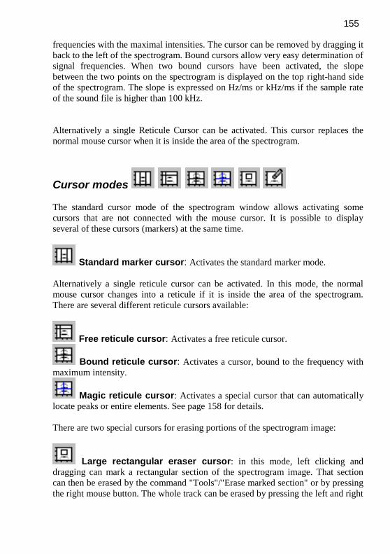
155

frequencies with the maximal intensities. The cursor can be removed by dragging it

back to the left of the spectrogram. Bound cursors allow very easy determination of

signal frequencies. When two bound cursors have been activated, the slope

between the two points on the spectrogram is displayed on the top right-hand side

of the spectrogram. The slope is expressed on Hz/ms or kHz/ms if the sample rate

of the sound file is higher than 100 kHz.

Alternatively a single Reticule Cursor can be activated. This cursor replaces the

normal mouse cursor when it is inside the area of the spectrogram.

Cursor modes The standard cursor mode of the spectrogram window allows activating some

cursors that are not connected with the mouse cursor. It is possible to display

several of these cursors (markers) at the same time.

Standard marker cursor: Activates the standard marker mode.

Alternatively a single reticule cursor can be activated. In this mode, the normal

mouse cursor changes into a reticule if it is inside the area of the spectrogram.

There are several different reticule cursors available:

Free reticule cursor: Activates a free reticule cursor.

Bound reticule cursor: Activates a cursor, bound to the frequency with

maximum intensity.

Magic reticule cursor: Activates a special cursor that can automatically

locate peaks or entire elements. See page 158 for details.

There are two special cursors for erasing portions of the spectrogram image:

Large rectangular eraser cursor: in this mode, left clicking and

dragging can mark a rectangular section of the spectrogram image. That section

can then be erased by the command "Tools"/"Erase marked section" or by pressing

the right mouse button. The whole track can be erased by pressing the left and right

156

mouse button while moving the cursor. Use this eraser mode for deleting larger

rectangular regions.

Standard eraser cursor: The mouse cursor will change into an eraser.

The shape of the eraser can be selected from the appearing tool set (

). The area under the cursor will be deleted once the left mouse

button is pressed. The undo button will undo the most recent erasing action. Use this eraser mode for deleting small or filigree regions.

The following three commands add specific frequency cursors in the standard

marker mode:

Insert bound frequency cursor Inserts a bound frequency cursors that moves along the peak frequency.

Insert frequency cursor Inserts a free-moveable frequency cursor.

Insert harmonic frequency cursor Inserts a harmonic frequency cursor.

Remove Marker The current marker in the spectrogram window is removed.

Remove Cursors Removes all cursors from the spectrogram window.

Erase marked section Erases the currently marked section of the spectrogram. Use this command to

remove unwanted sounds from the spectrogram image.

(Move reticule cursor by one pixel) / left, right, up, down These commands are accessible through keyboard shortcuts (e.g. arrow keys) only,

which have been defined from Tools/Keyboard Shortcuts and Popup Menu...

Copy cursor value Copies the current cursor measurement values into the clipboard (or transfers them

by DDE).

157

Copy the marker to the main window Copies the current marker of the spectrogram window to the main window

Cursor linkage between Instances In order to enable quantitative comparisons between different sound files, the

measurement cursors of several program instances can be linked. For this purpose,

several instances of the SASLab Pro software can be operated at the same time

(e.g. by the command File/”New Instance”).

When the desired dialog items are selected and several instances of SASLab Pro

are running, the corresponding cursors will move simultaneously in all instances,

where this cursor linkage has been activated.

Main window Marker duration The duration’s of the marked sections will be aligned between

instances.

Spectrogram window Frequency cursors The frequency cursors of the spectrogram window will be

aligned.

Marker duration The duration’s of the marked sections in the spectrogram

window will be aligned.

Spectrogram contrast The spectrogram contrast will be aligned.

Curve window X and Y Cursors The X and Y axis cursors will be aligned. Please note, that the

type of the one-dimensional transformations should be similar between instances.

Copy these settings to all other instances This option will automatically

copy the selections made to all other instances of the SASLab Pro software.

Display amplitude at reticule cursor cross If this option is activated, the amplitude [dB] at the cursor position is displayed on

the spectrogram image close to the cursor cross (for reticule cursors only).

158

Magic reticule cursor

The magic cursor mode supports searching local frequency peaks interactively.

Additionally, entire elements may be detected and their parameters (duration,

min, max frequency) can be measured automatically.

The magic cursor mode is activated by the command Tools/Cursors/Magic

reticule cursor or by the corresponding button . When the magic cursor is

placed over a narrow-band signal structure (e.g. a pure-tone whistle or a clearly

separated harmonic component), the peak (the frequency at maximum energy)

will be located automatically.

The parameter settings, that influence the behavior of this cursor, can be setup

from Tools/Cursors/Magic cursor setup… or the button .

Magic Cursor Setup

This dialog box defines the behavior of the magic reticule cursor.

snap distance : This value determines the distance between the current vertical

cursor position and a real peak in the spectrogram, at which the cursor would

then snap automatically. This distance is expected in pixels. The resulting

frequency interval is shown behind this edit field. If you need to investigate

single close-spaced frequency bands, this parameter should be set smaller than

the distance between these frequency bands. Larger values will make it easier to

locate peaks, because it is then not required to place the cursor so close to the

peak.

threshold : This absolute threshold limits the automatic peak detection

mechanism to regions, which exceed a certain amplitude. This threshold is

expected in dB relative to the full scale (0 dB corresponds to a full-scale or

maximum-amplitude signal). When setting this threshold to a low value (e.g. –40

dB) the magic cursor will be able to locate also low peaks. However, especially

in noisy recordings, this would lead to peaks within in the noise floor that are out

of interest. Therefore, it might be better to use a higher threshold. Higher

thresholds may of course prevent locating smaller peaks.

Locate and measure entire elements It this option is activated, the magic cursor will not only find the peak frequency

(and amplitude) at the current (horizontal) cursor position. Additionally, the

peak-search will be extended to the preceding and succeeding peaks around the

current horizontal cursor position.

159

By defining appropriate thresholds, this mechanism also allows to locate and

measure entire elements. The start and end of each element to be recognized is

derived from the amplitude across each potential element. The algorithm starts at

the maximum peak amplitude of the element and searches those points, where the

amplitude goes below a pre-defined threshold (start/end threshold). The resulting

points are assumed to be the start and end of each element. The corresponding

frequency measurements (f start, f end, f max, f min) are also taken from that

section.

This automatic recognition process will only work satisfying, if the signals to be

measured are relatively clearly structured and if they do not contain too much

noise or reverberation. The parameter settings made (snap distance, threshold,

start/end threshold) will also dramatically influence the success for a given class

of signals.

start/end threshold : This threshold determines the begin and end of the

automatically recognized elements. In contrast to the other threshold (described

at first), this one is related to the maximum peak amplitude of each element.

Therefore, 0 dB would correspond to the absolute amplitude of each peak and not

to a full-scale signal. Larger values (e.g. –10 dB) would lead to shorter element

duration estimates. Lower values (e.g. –20 dB) would provide longer elements.

exported measurements The following measurements can be exported by clicking the left mouse button.

The activated parameters will be copied into the clipboard (and optionally

transferred via DDE or saved into a LOG file if the appropriate setting are made

from File/Data Export/DDE Parameters / Log-File.

t start (absolute) : The absolute start time of the element in seconds.

t max (absolute) : The absolute time of the peak amplitude of the entire

element in seconds.

duration : The duration of the element in seconds.

peak amplitude : The peak amplitude of the entire element in dB (relative to

full-scale).

peak frequency : The frequency at the point of the maximum amplitude of the

entire element in Hz.

f start : The frequency at the start of the element in Hz.

f end : The frequency at the end of the element in Hz.

f max : The maximum peak frequency over the entire element in Hz.

f min : The minimum peak frequency over the entire element in Hz.

Please note, that the start and end of the elements are derived from the

spectrogram, which slightly over-estimates the duration of sound structures. This

over-estimation is caused by the smearing effect of the FFT window. This effect

160

will become significant in larger overlap settings. The amount of over-estimation

equals about half the duration of the FFT window (0.5 * FFT length / sampling

rate). It also depends on the window type and the frame size.

Copy headings This button copies an ASCII description of the currently activated measurements,

which may help in identifying the exported measurements.

mark detected element with a double cross If this option is activated, the recognized elements will be marked with two

vertical and horizontal thread-crosses showing both start/end and the

maximum/minimum frequencies. Otherwise, the element is marked with an

enclosing rectangle.

peak freq. Interpol. The peak frequency detection in the spectrogram is based on a maximum search

on the spectra. In order to increase the precision of the peak frequencies beyond

the spectrogram resolution, an interpolation algorithm is used. This parameter

determines the number of points used for interpolation. The option none will

inhibit the interpolation, which means, that the peak frequency resolution is equal

to the spectrogram resolution. The option auto will select the optimal number of

interpolation points for a given bandwidth. This interpolation will not be applied

to f start, f end, f max and f min (only to peak frequency).

161

Labels >

Labeling

The labeling feature allows adding labels to sound files. A label consists of a short

text (max 30 characters), a time stamp and a frequency stamp. Special section

labels have two time stamps (start and end of section) and no frequency stamp.

Labels are stored either directly into .wav file header or into separate data bank

files. The file format of these data bank files is the ASCII file format with *.LBL

extension. The data fields (coordinates and label text) are separated by tabulator

stop characters. Data sets (single labels) are separated by CR/LF. This file format

supports easy import into other applications like spreadsheets for further statistic

investigation. Therefore labels can also be used for measuring and data logging

purposes.

There are several display format options for labels:

Standard labels (time/frequency)

Alignment of the label text: left | center | right Style of label: text only | arrow | arrow & frame

Section labels (start/end time)

Vertical location of the label: layer1 | layer2 | layer3 | total The different layers allow to input overlapped or hierarchic labels. The total option

will draw large section boundaries occupying the total vertical display space.

In order to accelerate entering frequently-used text strings, it is possible to define

text modules from the main window command File/Rename by text module / Define text module that will also appear on the Text modules menu of the

Label dialog box (which can be accessed from the keyboard by pressing the Alt

and then the up/down arrow keys).

Existing labels can be edited by right clicking at the label. In the appearing dialog

box the label text, style and coordinates can be modified. The Copy button can be

used to copy the coordinates into the clipboard. In section labels the Play button

allows to playback the sound file section.

The proceed to next option will change the function of the OK button in such a

way that the Label edit box is not closed and instead its focus is set to the Next label, which can accelerate naming or renaming a whole set of labels. When the

focus of the Label edit box is switched to the next label, the corresponding

spectrogram view will also be moved to that next label. In addition to that, the edit

box will automatically proceed to the next label once one of the user-defined Text modules has been picked from the menu bar.

162

Labels can be moved by left clicking at the label and dragging while the left mouse

button is pressed. Section labels can also be resized by left clicking.

Right-clicking at a label while the Shift key is pressed will delete the label

immediately.

Insert label Inserts a standard label at the cursor position (time and frequency in the

spectrogram window; time only in the main and curve window). If the label is

inserted in the main or curve window, the frequency coordinate of the label is set to

-1.0, which means, that the frequency is not specified.

Insert section label Inserts a section label at the cursor position (time and frequency in the spectrogram

window; time only in the main and curve window). In contrast to the standard

label, a section label marks a time section by its start and end time coordinates.

Insert section label from marker Inserts a section label at the current marked section. In contrast to the standard

label, a section label marks a time section by its start and end time coordinates.

Section label grid... This dialog box allows activating an additional time-axis grid for each section

label. There are two grid options:

fixed interval duration : The distance between the grid ticks will be equal to the

specified time parameter. This option may be useful in order to get a more precise

visual impression of the section durations.

fixed interval count : There will be a fixed number of grid ticks for each

section, independently of the section duration. The specified number of ticks will

divide the section label into equally spaced sub-sections. This option may be used,

if investigations have to be made at time-standardized locations (e.g. for

characterizing whale signature whistles).

The two options can’t be combined. To disable the section grid at all, none of the

two options must be checked.

Label settings... This dialog box shows the current label settings and allows managing label files.

file name

Labels and titles are saved in separate *.LBL files. The file name of the currently

selected *.LBL file is displayed here.

163

lock labels If this option is checked, the existing labels cannot be moved or edited. Activating

this option may be useful to prevent unwanted modifications of labels.

auto save This listbox allows selecting the desired save/load option for labels and titles, when

a new sound file is opened or saved.

no saving: The labels are not saved and loaded automatically.

into extra .lbl file: If this option is selected, the corresponding *.lbl files are

loaded or saved automatically when a sound file is loaded or saved. When a sound

file is saved, the labels and the title are saved in a *.LBL file with the same file

name (except extension) and path as the sound file. When that sound file is opened

again, the corresponding *:LBL is opened automatically. This feature allows

simple label file assignment to diverse sound files.

Into .wav files: This option saves and loads the labels directly into/from the

current .wav file.

title This edit field allows inputting a title or a headline for the entire label file. That

title can be printed together with waveforms and spectrograms (see Export-

Parameters).

hide text If this option is checked, the label texts will be hidden. Activating this option may

be useful in situations, where many labels would overlap each other.

The large list box in the middle of the dialog box lists all labels with their

coordinates (time, frequency), label texts and formats. Single or several labels at

once can be edited from the bottom line. To do this first select the desired lines in

the list and make the modifications in the bottom line. Use the Enter button to enter

the changes into the list.

Display Moves the display area of the window, from which the Label settings dialog box

was launched, to the marked label. Alternatively, the label can be displayed by

double-clicking at the desired label on the list box.

Open... Opens an existent label file.

Save Saves the current labels under the currently selected file name.

164

Save As... Saves the current labels into a new file.

Copy

Copies the currently selected labels into the clipboard.

Select all Selects all labels in the list.

Select… Launches a dialog box that allows selecting the labels on the list by their label text

strings.

Sort by : time, text, layer Sorts the labels by time and replaces the label text by a running number. If the

dialog box option “label offset #” is checked, the renumbering procedure will start

with the specified number rather than 1.

Delete

Deletes the currently selected labels.

Enter

Enters the modifications made in the bottom line. Alternatively the Enter key of the

keyboard can be used.

Label statistics…

This dialog box displays some statistics on the temporal properties of the labels.

Min, max and mean of the intervals between the labels are calculated from all kind

of labels (both single-point and section labels), while the durations and the breaks

can only be determined for section labels. The break is measured from the end to

the start of the next section label. The measurements on section labels will only be

valid as long as they do not overlap. The measurements table can be exported

either via the clipboard (Copy button) or via a text file (Save button).

165

Additionally, a few more detailed diagrams can be selected from the diagram list

box:

histogram of intervals

histogram of durations histogram of breaks pulse density versus time This option counts the number of labels (both single-point and section labels) that

occur within each time frame (frame size = resolution).

duty cycle versus time This option determines the duty cycles (the normalized “on” time) for each time

frame (frame size = resolution). For instance, if there were a single section label

that lasts for 20 ms and falls entirely into a single time frame (resolution = 100

ms), then the duty cycle would be 20% in the time interval where the label is. All

other intervals were zero. In order to get smooth results, the resolution value

should be significantly larger than the durations of the labels. The duty cycle can

only be determined for section labels (single-point labels have no duration that

could be analyzed).

Use the >> button to display the selected diagram (OK will instead close the dialog

box and also launch the selected diagram).

The resolution edit box determines the temporal resolution of the diagrams.

Export label data… See page 101.

Automatic parameter measurements >

In the spectrogram window it is possible to measure time and frequency parameters

automatically. The spectrogram is scanned and single calls or song elements are

separated. That element detection is done by threshold comparison and a hold-time

mechanism. Then various parameters at certain locations within each of the

detected elements are determined. These locations can be start, end, center or the

point of maximum amplitude. At these locations peak frequency, amplitude at peak

frequency, bandwidth, quartiles or number of harmonics (peaks) can be

determined. Additionally, these frequency parameters may be derived from the

average spectrum of the entire element. All measured parameters will be displayed

166

graphically within the spectrogram. This allows tracking the operation of the

automatic parameter measurements and simplifies the process of finding the best

settings (thresholds and hold time). Optionally the measured parameters can be

displayed in a separated text window.

The settings for these measurements are defined on the command

”Tools”/”Automatic parameter measurements setup...” : Enable automatic measurements: Check this option to enable the automatic

parameter measurement.

Compute parameters from entire spectrogram: If this option is activated,

the measurements will be computed from the entire spectrogram file. Otherwise,

only the currently visible or marked section will be analyzed. When this option is

activated, it is necessary to use the OK or Update! button for updating the

measurement results after modifying the settings.

Automatic update: If this option is activated, the parameter measurement

display will be updated each time the spectrogram window is redrawn. Otherwise

the measurements are only displayed and updated when the OK or the Update! button is pressed. Note that the complete automatic update is suppressed if the

above option Compute parameters from entire spectrogram is activated.

Update Pressing this button will recalculate and update the Automatic Parameter

Measurements displays without leaving the setup dialog box. Use this button to

quickly check the current settings.

Copy results Copies the measurements into the clipboard (see also Copy

parameter measurement values ).

Add filename This option adds the name of the underlying soundfile to the report

table.

Show numeric results If this option is checked, the results will be displayed in

a separated display window.

Statistics Enable If this option is activated, statistics on the automatic parameter measurements will

be shown according to the settings made in the Automatic Parameter

Measurements Statistics dialog box. See page 188

167

Settings... This button launches the Automatic Parameter Measurements Statistics dialog box.

See page 188. Element separation

Element separation (segmentation) can either be accomplished by an automatic

threshold or spectral property based element detecting algorithm or manually by

marking the desired elements by section labels

automatic (single threshold) Select this option, if simple automatic threshold-

based element separation is desired. There is only one single threshold for both

element separation and element start/end locations. This option is useful, when the

single elements have similar amplitudes.

automatic (two thresholds) Select this option, if automatic threshold-based

element separation is desired and the single elements have different amplitudes. An

additional start/end threshold is used to determine both start and end of the

element detected by the primary Threshold. The option monotonic decreasing will accept only monotonously decreasing frequency courses in an

element, which can help rejecting echoes in bat calls.

automatic (three thresholds) This option is very similar to the above two thresholds option, except that two separate thresholds are being used for detecting

the start and the end of each element. This option might be useful for detecting bat

echolocation sweeps that start softly at high frequencies and end with a

reverberation tail. Due to strong reverberation tails, the two thresholds option

may prevent to detect the start of the calls precisely. The three thresholds mode

can be adjusted in such a way (a low threshold for the start and a higher threshold

for the end) that reverberated calls can be detected more accurately.

Threshold: If this threshold is exceeded, the start of a new element is registered.

When the signal goes below that threshold for at least the Hold time, the end of

that element is registered. In order to find the best threshold settings for the two or

three thresholds mode, the single threshold mode should be selected first. This

would allow to find an optimal setting for this primary threshold. The threshold is

correct, once all elements are recognized regardless whether the start and end

points are correct. The secondary start/end threshold can then be found after

switching into the two thresholds mode. The show threshold option allows

adjusting the threshold graphically by dragging its visual representation.

start/end threshold: This additional threshold is only valid for the two-

thresholds element separation mode. In this mode, for each element exceeding the

primary Threshold, the maximum amplitude is determined. The start and end of

the element are those points, where the amplitude goes below the start/end

threshold relative to the element maximum (for at least the hold-time). In this way,

168

the start and end of elements with different amplitudes will be recognized more

precisely. The threshold should be set to about –20 .. -10 dB, depending on the

structure of the elements. In recordings with high background noise, this secondary

threshold should not be set too low. The + and – buttons can be used to find the

best threshold setting incrementally.

relative to maximum: If this option is checked, the threshold comparison is

referenced to the most intensive point of the spectrogram. Otherwise, the threshold

value is interpreted as an absolute value related to full scale (0dB corresponds to

full scale = 1V peak amplitude).

show threshold: This option activates a graphic representation of the element

separation threshold, which helps to adjust the threshold.

total energy: If this option is activated, the threshold comparison is based on the

root mean square (total energy) of the spectra. Otherwise the peak amplitudes of

the spectra are compared. The total energy option should be activated for analyzing

multi-harmonic or noisy sounds because the peak amplitude is often too low for a

save element recognition.

Interactively (section labels) Select this option, if manual element separation

by section labels is desired. In this case each element to be measured must be

marked by a section label (command ‘Tools’/’Labels’/’Insert section label’). This

type of element separation may be useful for noisy signals, where automatic

detection is not satisfying. However, in many cases it may be useful to first use the

automatic separation and applying the command ‘Copy detected elements into

section labels’. These automatically scanned labels could then be modified

manually to match those elements, where the automatic process failed. The option

number labels automatically will replace the label titles by the number of the

corresponding element. If the spectrogram is printed later, these numbers will

appear on the printout as references.

automatic (whistle tracking) This element separation method is useful for

detecting soft whistle-like sounds in noisy sound recordings (certainly for

analyzing USV’s by laboratory mice and rats). The implemented algorithm

searches for steady signals having a relatively stable (peak) frequency course

without rapid frequency modulations. The amount of frequency modulation that

should be tolerated can be selected from the edit field max change. It is the

tolerated maximum change of the peak frequency between two consecutive time

bins on the spectrogram, expressed as the number of pixels on the spectrogram

(frequency bins). This setting therefore depends on the currently selected

spectrogram parameters (FFT length and overlap) and should be set to a value

between 1 and 4 pixels (depending on the time and frequency resolution of the

spectrogram). For best results, this parameter should be set to the smallest possible

value that still recognizes all the elements to be detected. The “whistles” button in

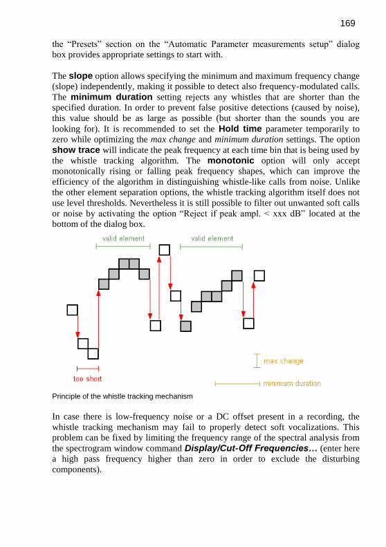
169

the “Presets” section on the “Automatic Parameter measurements setup” dialog

box provides appropriate settings to start with.

The slope option allows specifying the minimum and maximum frequency change

(slope) independently, making it possible to detect also frequency-modulated calls.

The minimum duration setting rejects any whistles that are shorter than the

specified duration. In order to prevent false positive detections (caused by noise),

this value should be as large as possible (but shorter than the sounds you are

looking for). It is recommended to set the Hold time parameter temporarily to

zero while optimizing the max change and minimum duration settings. The option

show trace will indicate the peak frequency at each time bin that is being used by

the whistle tracking algorithm. The monotonic option will only accept

monotonically rising or falling peak frequency shapes, which can improve the

efficiency of the algorithm in distinguishing whistle-like calls from noise. Unlike

the other element separation options, the whistle tracking algorithm itself does not

use level thresholds. Nevertheless it is still possible to filter out unwanted soft calls

or noise by activating the option “Reject if peak ampl. < xxx dB” located at the

bottom of the dialog box.

Principle of the whistle tracking mechanism

In case there is low-frequency noise or a DC offset present in a recording, the

whistle tracking mechanism may fail to properly detect soft vocalizations. This

problem can be fixed by limiting the frequency range of the spectral analysis from

the spectrogram window command Display/Cut-Off Frequencies… (enter here

a high pass frequency higher than zero in order to exclude the disturbing

components).

170

automatic (spectral entropy) This element separation method employs the

Wiener Entropy that can be used to detect tonal vocalizations in noisy recordings.

The Wiener Entropy (spectral flatness) is calculated by dividing the geometric

mean of the spectrum by the arithmetic mean of the spectrum and ranges

theoretically from 0 (pure tone signal) to 1 (white noise). An element is detected

each time when the entropy falls below the defined max entropy threshold. In

order to exclude unwanted short noise signals the min duration threshold on the

Post filter on elements section can be used (set the max entropy threshold to

1). Use the show trace option to visualize the trace of the entropy.

automatic (spectral bandwidth) This element separation method employs a

spectral bandwidth parameter that can be used to detect tonal vocalizations in noisy

recordings. The spectral bandwidth parameter is calculated by counting the most

intense number of frequency bins of the spectrum that represent a user-defined

fraction of the total energy of the spectrum. An element is detected each time when

the spectral bandwidth falls below the defined maximum number of frequency bins threshold. Note that the frequency bins threshold will be affected

by the analysis bandwidth of the FFT that is determined by the FFT size and the

windows type. In order to exclude unwanted short noise signals the min duration

threshold on the Post filter on elements section can be used (set the max entropy threshold to 1). Use the show trace option to visualize the trace of the

spectral bandwidth.

The edit> button creates section labels from the automatically detected elements

and switches to the interactive element separation mode. In this way it is possible

to edit the automatically detected elements, making it possible to label undetected

elements by pressing the Shift key and left-clicking at the desired start point in the

upper third of the spectrogram and dragging the mouse cursor to the end point. The

section labels can be resized and shifted by the mouse cursor or deleted by right-

clicking at them.

Hold time: In order to prevent cutting up of integral elements, a hold time can be

specified. If the amplitude of the spectrogram goes below the threshold for less

than this hold time, no new element is assumed. That option allows treating

complex elements with short silent sections as integral units. This parameter should

be set carefully in order to get a save element detection.

In order to exclude low frequency disturbance signals, an appropriate cut-off

frequency can be specified in the menu Display/lower Cut-Off Frequency.

171

Post filter on elements enable This option activates two additional filter criterions that can reject

unwanted sound elements that are shorter than the specified limit and/or that have a

broad frequency spectrum. This filter is certainly useful for eliminating short

(broad-band) cracks caused by the activity (movement) of caged animals. Note that

this option should be disabled during the process of optimizing the element

separation (adjusting thresholds and hold time), because this filter might

additionally disguise the operation of the primary element separation/detection

mechanism.

min duration: Elements shorter than this limit will be rejected.

max entropy: Elements whose minimum entropy is higher than this limit (weak

tonal structure) will be rejected. Tonal (whistle-like sounds) usually have a low

entropy (<0.3), while broad-band (noisy) sounds have higher entropies (>0.4). In

the process of optimizing the entropy threshold settings, it might be useful to

temporarily activate the Spectrum-based parameter entropy at Min param. of

entire element to get an idea of the entropy properties of both the wanted and

unwanted sounds.

Temporal parameters The temporal parameters are derived

from the spectrogram.

Duration of element: The duration

of each element from start to end is

measured.

Interval: The time duration from the

start of the preceding to the start of

the current element is measured.

Break: The silent interval from the

end of the preceding to the start of the

current element is measured.

Distance from start to max: The

distance from start to the location of

the maximum amplitude is measured.

Start/end time: The start and end time of each element is taken.

The additional option absolute will add the absolute time offset to the start/end

time. This absolute time offset is referenced to the start of the underlying sound

file. If the sound files have been recorded by Avisoft-RECORDER, then the time

offset is referenced to the start of the monitoring. In this way it is possible to get a

consistent time scale over subsequent (numbered) files.

Date The real-time date and time at the start of the element is copied into the

results listing. This information is derived from the file creation date.

more… > constant frequency (CF) section duration: The duration of the

constant frequency (CF) section of bat calls is measured. In order to get it work,

the location of the CF section (start, middle or end) within the bat call must

172

be selected and the frequency change threshold that should identify a CF

section must be specified.

Sub-elements The sub-element detection facility supports counting and measuring of elements

within phrases (groups of closely spaced elements), that are clearly separated in

time. This option will only work if the intervals between the consecutive sub-

elements are shorter than the intervals between the high-order elements (phrases).

The sub-element detection is based on a second hold-time, which has to be set to a

value shorter than the interval between sub-elements. The element separation hold-

time has to be set to a value longer than these sub-element intervals and shorter

than the interval between the high-order elements.

1 and 2 are the high-order elements (phrases) and 1:1, 1:2, 1:3 and 2:1, 2:2 are the

sub-elements. In this example the element separation hold-time was set to 0.1 s and

the sub-element hold-time to 0.01s.

Number of elements : The number of sub-elements within an element (phrase).

Element rate : The average rate of sub-elements within an element (phases). The

unit of the element rate is 1 second.

Hold time: This hold-time should be set to a value smaller than the intervals

between the consecutive (sub-) elements.

Note that the sub-elements option is not available with the element separation

method “automatic (whistle tracking)”. Use here instead the group analysis tool

(“Group. Anal.”).

Waveform parameters The waveform parameters are derived from the .wav file waveform and are

computed from the entire element.

rms : The root mean square either in 1 Volt or dB units in case the dB option is

activated.

energy : The energy of the element in 1 Volt2*sec units.

173

peak-to-peak ampl. :The peak-to-peak amplitude in 1 Volt units.

Group Anal. The group analysis option provides measurements on the

temporal (meta) structure of subsequent sound elements

that form groups (or phrases) that are separated by

significant breaks. In contrast to the Sub-elements option,

this option also provides detailed measurements on the

elements that form the group.

enable This option activates the group analysis mode.

The edit field ms defines the group hold time in milliseconds. Sound elements that

are closer than this duration will be grouped together. So, this group hold time

parameter should be larger than the longest break between the elements within the

groups and smaller than the silent breaks between the groups to be analyzed.

Settings… This button launches the Group Analysis Settings dialog that selects

the parameters to be measured:

Group Properties duration of group interval between groups (measured between consecutive group starts)

absolute time of group start and end element count (total number of element / group)

group index (running group number)

min/max parameters of all group elements If the “Min/Max param. of

entire element” options in the section “Location of measurements” have been

activated, this option will determine these parameters also over all elements in each

group.

Element Properties element index (running element number within the group)

relative time stamp (time interval from the group start to the start of the current

element)

separate groups by CR/LF characters : This option inserts an empty row

after each group (in the exported table).

Spectrum-based parameters The spectrum-based parameters are derived directly from the spectra of the

spectrogram.

174

Peak frequency: The frequency of the maximum amplitude of the spectrum.

Interpolation The peak frequency detection in the spectrogram window is based

on a maximum search on the spectra. In order to increase the precision of the peak

frequencies beyond the spectrogram resolution, an interpolation algorithm is used.

This parameter determines the number of points used for interpolation. The option

none will inhibit the interpolation, which means, that the peak frequency resolution

is equal to the spectrogram resolution. The option auto will select the optimal

number of interpolation points for a given bandwidth.

175

Fundamental frequency: This fundamental frequency detection option is based

on a peak search on the spectra of the spectrogram. The implemented algorithm

will detect the fundamental, even if the fundamental itself or single harmonics are

very weak or not present. In contrast to the Peak frequency option, which

returns the frequency at maximum amplitude, this option is immune against

varying amplitudes of harmonics in complex harmonic signals. See the description

of Number of peaks above and Frequencies of peaks for details on the

peak detection mechanism. Threshold and hysteresis for peak detection for the

fundamental frequency are the same as for the peak frequency search. Therefore,

these parameters can be edited from there. In complex (noisy) signals it may be

useful to first setup the peak detection algorithm using the Number of peaks above option. If all the peaks are detected properly, that option can be disabled

and the Fundamental frequency option can be activated.

Under some circumstances it might happen that the fundamental frequency

detection algorithm is disturbed by noise, which can then lead to an underestimated

fundamental frequency. This effect can be reduced by specifying a lower limit for

the fundamental frequency (usually one knows the lowest expected frequency).

The lower limit can be entered into the edit box labeled “>”

A fundamental frequency result of 0 Hz indicates that the detection algorithm

could not identify a valid harmonic structure (the detected peaks are not multiples

of a potential fundamental). In that case try to modify the peak search Hysteresis or

erase the noise components that might prevent a proper processing.

The option ACF activates the alternative autocorrelation method for the

fundamental frequency determination. Note that the autocorrelation method will

only work satisfying for low fundamentals (in relation to the sample rate). The

results will become more and more imprecise at higher frequencies.

Peak amplitude: The amplitude at the peak frequency (maximum of the

spectrum = peak amplitude).

Min frequency: That frequency, where the amplitude goes first below the

threshold (when we move from the maximum down to low frequencies), if the total

option is not activated. If the total option is activated, it is the frequency, where the

amplitude goes last below the threshold. See also illustrations below.

Max frequency: That frequency, where the amplitude goes first below the

threshold (when we move from the maximum up to high frequencies), if the total

option is not activated. If the total option is activated, it is the frequency, where the

amplitude goes last below the threshold. See also illustrations below.

total: This option determines the way how min, max and bandwidth is calculated.

If the total option is activated, the bandwidth will cover all peaks that exceed the

176

threshold. Otherwise, the bandwidth will only cover the maximum peak exceeding

the threshold.

Min and Max frequency detection with the total option activated.

Min and Max frequency detection with the total option not activated.

Bandwidth: Difference between Max frequency and Min frequency.

Threshold: This threshold is used for the bandwidth, min and max frequency

calculation. The threshold is referenced to the peak amplitude. An additional

threshold can be activated from the associated checkbox below the primary

threshold edit field:

Quartiles: These parameters characterize the distribution of energy across the

spectrum. The spectrum will be integrated and divided into four equal parts. The

three frequencies dividing the magnitude spectrum into four parts are called

quartiles:

Quartile 25%: below this frequency is 25% of the total energy.

Quartile 50%: The mean frequency of the spectrum. Below this frequency is 50%

of the total energy.

Quartile 75%: Below this frequency is 75% of the total energy

The distance between quartile 75% and quartile 25% is a measure of the pureness

of the sound.

177

Entropy: The Wiener entropy parameter allows to quantify the randomness (or

pureness) of sounds. It is the ratio of the geometric mean to the arithmetic mean of

the spectrum. This parameter is (theoretically) zero for pure-tone signals and one

for random noise. Because of the properties of the short-time FFT (its analysis

bandwidth is always greater than zero), the value will not be exactly zero for a pure

tone signal. The absolute results will depend on FFT length, frame size and

window type. Therefore, the entropy parameter should only be used for

comparisons among spectrograms generated using the same spectrogram parameter

settings.

Harmonic-to-noise ratio: The harmonic-to-noise (HNR) parameter quantifies

the ratio of harmonic to nonharmonic energy. The noise floor of the spectrum is

estimated by calculating the moving average of the spectrum. The maximum

distance between the original spectrum and the filtered spectrum (expressed in dB)

is taken as the HNR measure. The width of the averaging window can be defined

by entering the number of frequency bins. Note that the HNR estimation is

affected by the FFT size, the evaluation window type and the number of the

averaging frequency bins.

Number of peaks above dB: The number of peaks (harmonics) exceeding

this threshold is counted. The threshold is related to the maximum peak.

Frequencies of peaks: The frequency of each peak is determined.

Amplitudes of peaks: The amplitudes of each peak are determined.

max peak entries: This value limits the maximum number of peaks in the output

file. This value should be set to the expected number of peaks.

Hysteresis for peak detection: This value is used for peak detection. Only

peaks that are higher than the preceding valley plus this hysteresis will be detected

as peaks.

178

uniform parameters for all locations If this option is activated, the selected “Spectrum-based parameters” will be taken

at all selected “Locations of measurements”. Otherwise, the spectrum-based

parameters can be defined separately for each location, which would allow to

exclude unwanted combinations of certain parameters and locations. The list box

“Location” allows to navigate through the various locations.

Locations of measurements

The parameters listed above can be computed at different locations within the

element:

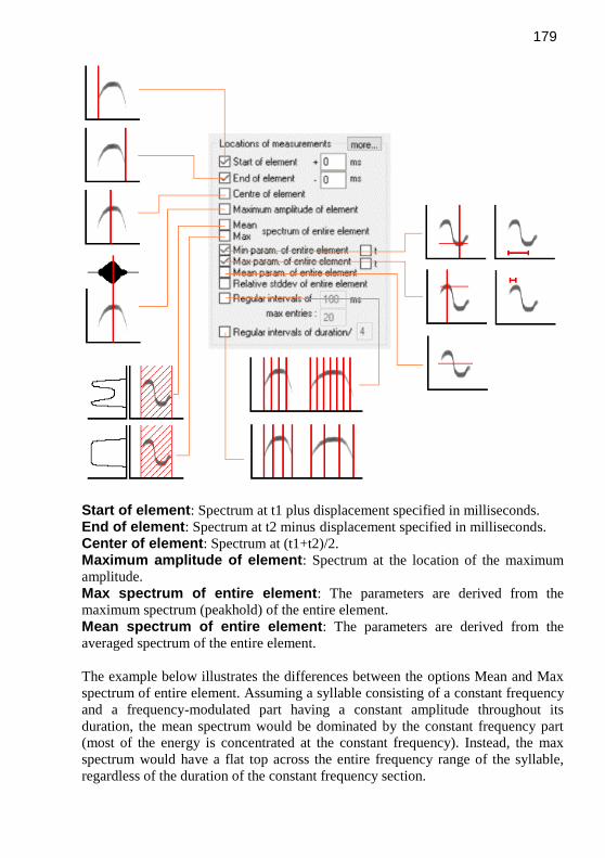
179

Start of element: Spectrum at t1 plus displacement specified in milliseconds.

End of element: Spectrum at t2 minus displacement specified in milliseconds.

Center of element: Spectrum at (t1+t2)/2.

Maximum amplitude of element: Spectrum at the location of the maximum

amplitude.

Max spectrum of entire element: The parameters are derived from the

maximum spectrum (peakhold) of the entire element.

Mean spectrum of entire element: The parameters are derived from the

averaged spectrum of the entire element.

The example below illustrates the differences between the options Mean and Max

spectrum of entire element. Assuming a syllable consisting of a constant frequency

and a frequency-modulated part having a constant amplitude throughout its

duration, the mean spectrum would be dominated by the constant frequency part

(most of the energy is concentrated at the constant frequency). Instead, the max

spectrum would have a flat top across the entire frequency range of the syllable,

regardless of the duration of the constant frequency section.

180

Min param. of entire element: The parameters are internally computed for all

instantaneous spectra between the start and the end of each element. The minimum

of the measurement values throughout all these spectra is determined. For instance,

when applied to the peak frequency, the "min param of entire element" will return

the lowest peak frequency within each element. Similarly, when applied to the

entropy, it will return the lowest entropy that occurred between the start and end of

each element. The option t will additionally measure the location of the minimum

within the element.

Max param. of entire element: The parameters are internally computed for all

instantaneous spectra between the start and the end of each element. The maximum

of the measurement values throughout all these spectra is determined. For instance,

when applied to the peak frequency, the "max param of entire element" will return

the highest peak frequency within each element. Similarly, when applied to the

entropy, it will return the maximum entropy that occurred between the start and

end of each element. The option t will additionally measure the location of the

maximum within the element.

Mean param. of entire element: The parameters are internally computed for

all instantaneous spectra between the start and the end of each element. The mean

value of all these individual measurement values is calculated and put out.

Mean param. of entire element applied to the Peak frequency

181

Relative stddev of entire element: The parameters are internally computed

for all spectra between the start and the end of each element and the relative

standard deviation ( = standard deviation / mean value) of these parameters is

calculated. This parameter can be used for instance for quantifying frequency or

amplitude modulation.

Regular intervals of: The parameters are computed repeatedly at regular

intervals within each element. The interval is specified in milliseconds. The time

resolution of the spectrogram must be adapted to the desired measurement interval.

The maximum number of samples within each element will be limited to the

specified max entries.

Regular intervals of duration / n: The parameters are computed repeatedly at

regular intervals within each element. The number of measurements taken per

element is specified here. This means, that the time interval will depend on the

duration of each element.

more… : This button launches a separate dialog box for selecting additional

parameters:

Time derivative of entire element This section provides parameters that are

based on the time derivative of the spectrum-based parameters. Currently, only the

Peak frequency and the Fundamental freq. are supported.

sum : The sum (integral) of the time derivative over the entire element is

calculated (corresponds to the frequency change from the start to the end).

mean : The mean of the time derivative over the entire element is calculated. If

the option calculate slope (kHz/ms) is checked, this measure represents the

average slope of the element expressed in kHz/ms.

min : The minimum of the time derivative over the entire element is calculated. If

the option use absolute values is checked, the minimum absolute value is

determined. Otherwise, the largest negative (descending) change will be provided.

If the option calculate slope (kHz/ms) is checked, the change is expressed in

kHz and referenced to a time interval of 1.0 ms (unit kHz/ms). The option t provides the time offset where the minimum was detected (expressed in seconds

relative to the start of the element) and the option f similarly provides the

corresponding frequency.

max : The maximum of the time derivative over the entire element is calculated. If

the option use absolute values is checked, the maximum absolute value is

182

determined. Otherwise, the largest positive (ascending) change will be provided. If

the option calculate slope (kHz/ms) is checked, the change is expressed in kHz

and referenced to a time interval of 1.0 ms (unit kHz/ms). The option t provides the

time offset where the maximum was detected (expressed in seconds relative to the

start of the element) and the option f similarly provides the corresponding

frequency.

use absolute values : If activated, the min and max will be calculated from

the absolute values of the time derivative.

calculate slope (kHz/ms) : If activated, the mean, min and max are expressed

in kHz and referenced to a time period of 1.0 ms (the frequency change between

the spectrogram time bins is divided by the time interval between those two bins).

distance for calculating differences : xxx time bins : This setting

determines the distance between the spectrogram time bins from which the

frequency change is calculated. Due to the limited frequency resolution of the

spectrogram, it is sometimes (depending on the FFT length and overlap settings)

required to increase this distance in order to get meaningful results for signals that

exhibit a slow frequency change. Note that a large distance value will prevent to

calculate the time derivative at the margins of the element. If one is interested in

the amount of frequency change in rapid frequency jumps, the distance should be

set sufficiently high and the option calculate slope (kHz/ms) must be deactivated

in order to measure the frequency difference properly. second time derivative: This section allows to analyze the second time

derivative in order to localize reversal points within the frequency contour. The

mechanism is similar to the first time derivative described above.

limit the analysis to the final xx % of the element: If activated, the time

derivative analysis will be limited to the selected final percentage of each element.

In conjunction with the max f option and the 40% setting, it is possible to measure

the “characteristic frequency” (frequency of the call at its lowest slope toward the

end of the call), which is commonly used for identifying bat species.

show time derivative plots : This option displays the time derivative function

from which the above parameters are calculated.

Reject if peak ampl. < … dB When this option is activated, the spectrum-based

parameters will be rejected at those locations where the peak amplitude of the

corresponding spectrum is lower than the specified threshold. If the rejection

threshold has been adjusted properly, this option can certainly improve the

183

reliability of the parameters peak freq(minentire) and peak freq(maxentire) in

sound elements that exhibit short silent breaks (which would otherwise cause

wrong results).

The unit of all time-parameters is seconds. The unit of the frequency parameters is

Hz.

Exclude rejected elements from results table If activated, the elements

rejected by the above option will be excluded completely from the results table.

Otherwise, they will still appear on that list.

Derived element-based parameters

In order to extend the classification facilities it is possible to derive more complex

parameters from the original measurements for each detected element. A common

task is to compare peak frequencies at different locations (start and end), which

allows distinguishing between upward and downward frequency modulated

elements.

Up to two derived parameters can be activated (derived parameter #1 and #2).

The derived parameters are computed from the difference of two parameters. The

parameter selected on the second line is either subtracted from (-), divided by (/) or

added (+) to the one specified on the first line. The + option will additionally

divide the result by two in order to provide the mean value.

If the option divide by duration is activated, the difference of the two

parameters is divided by the duration of the element. This may be useful if you are

interested in measuring the rising velocity [Hz/s] of frequency-modulated elements

(select the peak freq parameter and start versus end location).

If the option absolute value is activated, the absolute value of the difference will

be taken. The name edit field defines the name of the derived parameter that is

displayed on the results table.

Note that several combinations of parameters and locations will not make sense

(e.g. subtracting time parameters from frequency or class parameters). So it is up to

the user to select meaningful combinations.

Show graphic results: If this option is activated, the results of the spectral

measurements will be displayed on the spectrogram. add filename : If activated, the name of the current sound file will be added to

the results list. The related option each row will add the filename to every row –

184

otherwise it will only be added to the first (element) row. The option with path

will include the entire pathname.

Presets whistles : selects appropriate default settings for pure-tone, whistle-like

vocalizations

barks : selects appropriate default settings for noisy barks

Classification

Enable If this option is activated, a classification of detected will be made according to the

settings made in the Classification Settings dialog box. See page 184.

Settings... This button launches the Classification Settings dialog box. See page 184.

Response This button launches the Automatic Response Settings dialog box. See page 195.

Classification

Based on the measured parameters, the detected sound elements can also be

classified automatically. For this purpose, a set of element classes can be defined.

There are two classification methods available: Axis-parallel thresholds A class is represented by one parameter interval for each of the activated

parameters. If a detected element satisfies all the parameter criterions of one of

these classes, this element will be associated to that particular class.

Linear discriminant analysis For each pre-defined class a linear discrimination function score is computed:

Si = ci + wi1*x1 + wi2*x2 + ... + wim*xm

In this formula, the subscript i denotes the respective class; the subscripts 1, 2, ...,

m denote the m parameters; ci is a constant for the i'th group, wij is the weight for

the j'th parameters in the computation of the classification score for the i'th group;

xj is the observed value for the respective case for the j'th variable. Si is the

resultant classification score. The maximum classification score Si will determine

the class associated to the element.

185

Both classification mechanisms may be used for note type classification or species

discrimination. The number of elements associated to each class can be counted

automatically for statistics purposes.

Classification Settings

This dialog box allows defining the classes for the classification process.

Class : This combo box selects the class to be defined. Each class is identified by its name

listed in this field.

add class Use this button to add a new class to the configuration. The title of a class can have

up to 30 characters.

rename Use this button to rename the selected class.

delete Use this button to remove the selected class from the configuration.

Location This combo box selects the location of measurements to be edited. The list contains

all locations activated in the Automatic Parameter Measurements setup dialog box

(except Regular intervals of, which is not available for classification)

The parameter list below the Location combo box shows all activated parameters

(except Interpulse interval, Absolute time, Frequencies of peaks and Amplitude of

peaks, which are not available for classification).

For the axis-parallel thresholds method:

The edit fields below from and to define the value range limits, which should be

specified for each class and each location. The unit and scale of these values is the

same as in the numeric Automatic Parameter Measurements display window (1s,

1Hz or 1dB). If you don’t enter any value into a field, the associated parameter

comparison will be ignored (don’t care). If there is more than one parameter

activated, all of the specified criterions must be satisfied to sort an element into this

class (logic AND combination). If you need an OR combination, an additional

class with the same title could be created.

186

For the discriminant function mode:

The edit fields below weight define the weights for each parameter in the

classification function.

Copy settings This button copies the current classification settings for all classes into the

clipboard (in TAB-delimited ASCII format). This settings listing could be pasted

from a spreadsheet application to see an overview of the entire settings.

Save This button saves the current classification settings for all classes into a *.cls file

(TAB-delimited ASCII format).

Open Opens a previously saved *.cls file. If there are parameters in the loaded file, which

are not active in the current settings of the Automatic Parameter Measurements,

these parameters will be activated automatically. The *.cls files could be edited

manually (e.g. in Excel). However, the headline on the first row should not be

altered. The HT delimiters between the data fields must be preserved. Additional

rows may be added. The Open command can also be invoked by drag&drop.

Import This command is equivalent to the Open command, except that the parameters,

stored in the *.cls file, will not be activated automatically. In other words, the

Import command only takes those parameters from the file that have already

activated in the current configuration. The Import command can also be invoked

by drag&drop while the shift key is pressed.

The Save and Open/Import commands may be useful for efficient handling of

different classification settings. Please note, that the classification settings are also

saved into the SASLab configuration file (*.ini). Therefore, switching between

classification settings could also be done by using different configuration files.

Reset Resets the parameter limits for all classes and locations.

187

Configuring the classification option

First enable the Enable classification option in the Automatic Parameter Measurements settings dialog box and launch the Classification settings

dialog box by the Settings button.

1. Select the desired classification method (axis-parallel thresholds or

linear discriminant function)

2. Add the title for the new class by clicking at the add class button.

3. Select the Location, for which you want to input the value range limits

(if you have activated more than one location in the Automatic Parameter

Measurements dialog box).

4. Input the classification parameters:

For the axis-parallel thresholds method:

Input the lower (from) and upper (to) limits for each parameter at all locations. If

one limit is out of interest (don’t care), leave the corresponding field(s) empty.

Repeat this procedure (goto 2, add class button) until you have defined all

classes you need.

For the linear discriminant function method:

Input the constant and the weights for each parameter at all locations for the

discriminant function. When specifying a threshold, the samples will only be

classified to one of the pre-defined classes when the classification score Si exceeds

this thresholds. Leave this edit field empty if no threshold exclusion is desired.

When the option use min(abs(score)) is activated, the classification criterion is

the smallest absolute value of the classification scores (instead of the maximum).

This option may be useful for situations, where the standard linear discriminant

approach with looking for the maximum score does not work. Assuming you need

to classify elements based on a single parameter (e.g. the dominant frequency) into

more than two classes. When setting the constant to the group centroid (the mean

dominant frequency of each class) and the weight to –1.0, the samples will be

classified successfully (you would get similar results when using the axis-parallel

thresholds option with appropriate interval settings, but the discriminant function

method will be easier to setup).

5. Repeat this procedure (goto 2., add class button) until you have defined all

classes you need.

The specified limits (or the constants and the weights for the discriminant

functions) can be edited later by selecting the corresponding Class and Location

entries. For complex settings use the Copy settings button to see an overview

188

display of all classes and locations by pasting this overview into a spreadsheet.

Additionally, the classification limits of each class can be seen on the 3D-

Scatterplot view, which can be activated from the statistics setup dialog box.

Please note, that the classification settings will be lost, once the parameter or

location selections in the Automatic Parameter Measurements setup have changed.

Automatic Parameter Measurements Statistics

This dialog box allows selecting the statistics display for the activated parameters

of the Automatic Parameter Measurements facility.

Numeric display The overall statistic values selected in this section will be displayed for each

parameter at each location over all detected elements. The numeric display will

appear on the top of the Automatic Parameter Measurements display window.

The following statistics are available:

Minimum, Maximum, Mean, Median, Standard deviation Relative on time (for duration only) The relative on time corresponds to the sum of the element durations divided by

the total duration of the spectrogram (the option “Compute parameters from entire

spectrogram must be activated”).

Histogram of one parameter This section allows choosing one parameter and a single location, from which a

graphic histogram display is generated.

Enable Check this option to enable the histogram display. Note, that the

Statistics/Enable option in the Automatic Parameter Measurements must be

activated also.

Parameter : This list-box selects the parameter to be displayed.

Location : Selects the location (within each element) from which the selected

parameter should be displayed.

Resolution This edit-box defines the x-axis resolution (width of the classes) of

the histogram. The unit of this value is 1 s for all temporal parameters and 1 Hz for

all frequency parameters. This value has no meaning for the class parameter.

189

2D-Scatterplot of two parameters A two-dimensional scatterplot of two parameters/locations is generated.

3D-Scatterplot of three parameters A three-dimensional scatterplot of three parameters/locations is generated. This

display is a powerful tool for quickly exploring dependencies between parameters.

3D orientation is supported by animated or mouse controlled modification of the

viewing perspective. The perspective can be changed manually by left clicking and

dragging. The animated perspective view can be activated by right clicking on the

graph.

Update Updates the Automatic Parameter Measurements results.

Copy parameter measurement values Copies the parameter measurement values of the marked or visible section into the

clipboard. Optionally these values will be transferred by DDE or will be written

into a LOG file (File/DDE Parameters / Log-File).

Copy parameter measurement values for entire file Copies the parameter measurement values of the entire spectrogram (spectrogram

(not only the visible section) into the clipboard. Optionally these values will be

transferred by DDE or will be written into a LOG file (File/DDE Parameters / Log

File, see page 139).

Copy parameter measurement values in transposed order Copies the parameter measurement values that are currently visible on the numeric

display window in transposed order (rows and columns reversed) into the

clipboard.

Copy parameter measurement headings Copies the headings for the currently activated parameters into the clipboard. This

supports navigation through the exported measurement values. Optionally these

headings will be transferred by DDE or will be written into a LOG file (File/DDE

Parameters / Log-File).

Save detected elements into numbered .wav files This command will save each detected element into a separated numbered .wav

file. The file name format is Txxxxxxxx.WAV.

190

Destination base directory : This edit-field specifies the base directory, where

the numbered .wav files will be saved.

Filter : This list-box determines, how and which events will be saved.

The option all classes will save all events into the specified directory, regardless

of any class attributes.

The following options are only available, if the classification facility is activated:

The option sort by class will save the elements sorted by their class attributes

into separated sub-directories relative to the specified base-directory. The sub-

directory names will be derived from the class names (only the first 8 characters

will be used).

The following options only ..., representing the defined classes, will only save

those elements, which are associated with these classes.

File margins : It is possible to add a short margin before and after the detected

element before it is saved into the .wav file. The duration of that margin is

specified in units of 1 s.

Remove gaps between detected elements This command will remove the gaps between the detected elements from the sound

file. The resulting new sound file (displayed in the main window) will only contain

the detected elements. Please note that the original sound file displayed in the main

window will be replaced by the resulting file.

Filter : This list-box determines, which events will be preserved

The option all classes will preserve all events, regardless of any class attributes.

The following options only ..., representing the defined classes, will only preserve

those elements, which are associated with these classes. This option is only

available, if the classification facility is activated.

margins : It is possible to add a short margin before and after the detected

element before the gaps are removed. The duration of that margin is specified in

units of 1 s.

Insert break marks If this option is activated, a short click will be inserted

between the preserved elements. This will allow you to identify the original bounds

of the original elements.

Copy detected elements into section labels This command will generate a section label from each detected element.

191

Filter : This list-box determines, which events will be copied to the label list.

The option all classes will copy all events, regardless of any class attributes.

The following options only ..., representing the defined classes, will only copy

those elements, which are associated with these classes. This option is only

available, if the classification facility is activated.

File margins : It is possible to add a short margin before and after the detected

element before it is copied to the label list. The duration of that margin is specified

in units of 1 s.

Label text This section determines the label texts of the generated labels.

index The label text will contain the consecutively index of elements.

class name The label text will contain the name of the element class (if there are

any).

delete all previous labels If this option is checked, the previously defined

labels will be deleted.

Copy peak frequencies into labels Labels indicating the peak frequencies at the selected Location of measurements

will be created. The last label of each element will be marked with a dot (period) in

the label text. This enables the subsequent grouped export of labels

(Tools/Labels/Export label data…). In this way, it is for instance possible to

export frequency contours that have been edited manually (the created labels can

be moved prior to exporting them).

Keyboard Shortcuts and Popup Menu This command allows defining keyboard shortcuts for all menu commands of the

selected window. Additionally, each command can be added to the popup menu,

which is activated by right clicking on the window. To modify a keyboard shortcut,

first select the command on the list and then activate the desired shortcut on the

bottom of the dialog box. In order to simplify the access to frequently used

commands, it is recommended to use appropriate shortcuts or popup menu entries

for these commands.

WavFile

This menu supplies functions that are also available from the main window.

Open... Opens a new sound file.

192

Browse Rename Rename by text module These commands are duplicates of the corresponding main window commands on

the File menu.

Import Format Sets the import format for the Open command (See 35).

Spectrogram parameters... Sets the spectrogram parameters (See page 44).

Copy : Copies the currently visible or marked section of the .wav file into the clipboard.

Save As… Saves the currently visible or marked section of the .wav file into a new .wav file.

New instance Starts a new instance of Avisoft-SASLab Pro.

Save configuration Saves the current configuration (parameter settings) into the currently active

configuration file (*.ini).

Automatic Parameter Measurements display window The results of automatic parameter measurement can be shown in a separated

display window. That window can be enabled in the setup dialog with the Show

results in numeric format option.

All parameters selected in the setup dialog will be displayed in a table. The

measurement values of each element are separated by vertical lines. The element

number is displayed in the first column. The second column indicates the location

of the following frequency parameters within each element.

Double-clicking at a list entry will move the spectrogram view to this element.

193

Setup

The Automatic parameter measurements setup dialog is launched

Classification settings... See page 184.

Statistics settings.... See page 188.

194

Compute parameters from entire spectrogram If this option is checked, the automatic parameter measurements will be executed

on the entire spectrogram file (not only on the marked or visible section). The

element numbering is independent from the visible or marked section and will start

at the first element of the spectrogram file. Otherwise the parameter measurements

will only be executed on the marked or visible section of the spectrogram file.

Element numbering will start at the first element of the marked or visible section.

Export Copy parameter measurement values Copies the parameter measurement values of the marked or visible section into the

clipboard. Optionally these values will be transferred by DDE or will be written

into a LOG file (DDE Parameters / Log-File).

Copy parameter measurement values for entire file Copies the parameter measurement values of entire spectrogram (not only the

visible section) into the clipboard. Optionally these values will be transferred by

DDE or will be written into a LOG file (DDE Parameters / Log-File.

Copy parameter measurement values in transposed order Copies the parameter measurement values that are currently visible on the numeric

display window in transposed order (rows and columns reversed) into the

clipboard.

Copy parameter measurement headings Copies the headings for the currently activated parameters into the clipboard. This

supports navigation through the exported measurement values. Optionally these

headings will be transferred by DDE or will be written into a LOG file (

DDE Parameters / Log-File).

Copy the time stamp of the selected element Copies the time stamp of the selected element into the clipboard.

Copy class sequence Copies the names of the detected classes into the clipboard (in ASCII format).

Example: A B B A C C C B

Copy class frequency The number of elements associated to each class is counted. The result is copied

into the clipboard (in ASCII format).

Example:

195

A 2

B 3

C 3

n= 8

Save detected elements into numbered .wav files... See page 189.

Remove gaps between detected elements from sound file... See page 190.

Copy detected elements into section labels See page 190.

DDE Parameters / Log-File. Launches the DDE parameters dialog box. See page 139.

View Show the selected element on the spectrogram window This command

moves the spectrogram window view to the element that is currently selected on

the list.

Synchronize the numeric and the spectrographic view. This option

connects the scroll bars of the numeric and the spectrographic display views.

Automatic Response

The Automatic Recording option of the Real-Time Spectrograph and the

Automatic Parameter Measurement / Classification option can be combined in

order to immediately generate an Automatic Response to acoustic events

depending on the recognized class of event. Responses can be either simple

playbacks of pre-recorded .wav files or more complex modified echoes of the

original sound event. This feature enables sophisticated playback experiments for

investigating animal communication.

The Automatic Response Settings dialog box allows defining the desired response

for each class:

196

The listbox on the top of the dialog box lists all available classes. Additionally

there are entries for unrecognized elements ‘?’ and wildcard ‘*’ responses. To

specify the response for a class select the corresponding line on the list and select

the type of action from the Action listbox. If the action specified for the wildcard

* class is not no response, this action will override any other actions specified on

the other classes. Some actions require to input a filename or another text string as

parameter.

The following response actions are available:

no response : No response will be generated.

play .wav file : The specified wav file will be played back.

run another program : The specified program will be executed. This option

could be used to run customized programs in order to realize special responses (by

remote- controlling external systems via IO interfaces: e.g. triggering a feeding

automat for learning experiments or switching light on or off). If the option

Append file name is activated, the file name of the underlying .wav file is added

as a command line argument. The option Append channel number will add the

channel number to the command line enabling multi-channel operation.

DDE transaction XTYP_POKE : DDE transaction XTYP_EXECUTE : A command or data string is sent to another application through Dynamic Data

Exchange. SASLab acts as a DDE client with the wType parameter set to

XTYP_POKE or XTYP_EXECUTE. The DDE parameters for this transaction are

defined on the parameter field (instead of a filename) as follows: Application; Topic; Item; Data/Command string

The semicolons act as delimiters between the DDE parameters. Please note, that

the DDE parameters for this response action are completely defined on the

parameter field. The separated DDE Parameters / Log File dialog is used for

measurement data export only. The DDE transaction facility allows the user to

program more individual responses (e.g. by a Visual Basic program receiving these

DDE commands). If the option Append file name is activated, the file name of

the underlying .wav file is added to the data/command string. The option Append channel number will add the channel number to the data/command string

enabling multi-channel operation.

echo The original sound event will be played back.

echo, Reverse The reversed event will be played back.

197

echo, Change Volume The original sound event is modified according to the

settings made in the Edit/Change Volume command.

echo, FIR filter The original sound event is filtered according to the settings

made in the Edit/Filter/Time domain FIR-Filter command.

echo, IIR filter The original sound event is filtered according to the settings made

in the Edit/Filter/Time domain IIR-Filter command.

echo, FFT filter The original sound event is modified according to the settings

made in the Edit/Filter/Frequency Domain Transformation command.

echo, Time/Pitch Conversion The original sound event is pitch converted

according to the settings made in the Edit/Format/TimePitch Conversion

command.

resynthesis, Scale The spectrogram is first scanned for the fundamental

frequency and amplitude envelope according to the setting made under the

Synthesizer command Tools/Scan Spectrogram (f0, a0). The fundamental

frequency and amplitude envelope will then be modified according to the settings

made under the ToolslScale command. This feature allows modifying the

fundamental frequency without changing the temporal properties or modifying the

speed without changing the fundamental frequency.

resynthesis, add parameter from .ARR file The spectrogram is first scanned

for the fundamental frequency and amplitude envelope according to the setting

made under the Synthesizer command Tools/Scan Spectrogram (f0, a0). The

synthesizer parameters (amplitudes of harmonics or amplitude and frequency

modulation) stored in the specified .arr file will then be added to the arrangement.

This feature allows adding harmonics or modulations to whistles.

increment RECORDER file number The current .wav file number of Avisoft-

RECORDER is incremented. This option allows filtering the events saved by the

RECORDER. For this mechanism it is required, that the Increment option of the

RECORDER configuration is not activated. Additionally, the Autotransfer to SASLab and Wait for Avisoft-SASLab options must be activated. With the

appropriate classification settings in SASLab Pro, the RECORDER will then only

save those events, which contain at least one element of the associated class.

The select file button can be used to search for the parameter files.

The echo and resynthesis actions require, that the original sound event is loaded

into the main window. Therefore, the Automatic Recording option Autotransfer

198

event waveform must be activated for these actions. For all other actions it is

sufficient to activate the Autotransfer event spectrogram option.

Delay The response is delayed by the specified duration.

Repeat x times The responses are repeated according to this entry.

Append file name If this option is activated, the complete .wav file name will be

appended to the actions run another program and DDE transaction XTYP_POKE /

XTYP_EXECUTE . The format is as follows:

/file=xxxx

example: “ /file=C:/RECORDER/CHANNEL1/T0000001.WAV”

Append channel number If this option is activated, the channel number of the

.wav file will be appended to the actions run another program and DDE

transaction XTYP_POKE / XTYP_EXECUTE . The channel number is extracted

from the path name of the .wav file. The path name must include the string

“channel” followed by the channel number. For example, channel number one

should have the string “channel1” in its path name.

The format is as follows:

/channel=x

example: “ /channel=1”

Send acknowledge to Avisoft RECORDER If Avisoft-RECORDER is used

as recording front end, it may be useful to establish some kind of handshaking

between RECORDER and SASLab. Otherwise endless loop situations may occur,

because played responses can trigger the RECORDER again. Therefore this option

should be activated, when Avisoft-RECORDER is used. Additionally, within the

RECORDER configuration dialog the option Wait for Avisoft SASLab must be

activated. Using Avisoft-RECORDER as recording front-end has several

advantages over Automatic Recording option of the SASLab Real-time

spectrogram. You will have much more control over the critical event detection

(pre-trigger and graphic adjustment of trigger conditions).

Play response through Avisoft RECORDER If this option is activated, all

playback responses will be routed via the Avisoft RECORDER software. This

would enable ultrasonic playback by using a high-speed data acquisition / playback

board.

Enable Automatic Response Enables the Automatic Response mode.

Additionally, the real-time spectrograph command Record/Automatic

Recording/Autotransfer Event spectrogram or waveform, the main window option

Actions/On new sound file/Create Spectrogram and the Enable automatic

199

measurements option from the Automatic parameter measurements setup must be

activated in order to make the complete response process working.

When the Automatic Response mode is activated, the measurements will be

automatically be exported (copied into clipboard, transferred via DDE or written

into a LOG file) Use the DDE/LOG button to activate DDE or LOG file data

export. This may be useful for protocol purposes during long-term monitoring.

Prepare By pressing this button, all settings necessary for setting-up the

Automatic Response option feature will be made at once.

Methods of measurement value export

Avisoft-SASLab Pro offers several ways for exporting measurement values for

subsequent statistical analysis:

Clipboard A single data-record is copied into the clipboard. To save this record you have to

switch to a different application where the data can be inserted. To prevent the

time-consuming redrawing of application windows you should arrange the

windows so that they do not overlap. Because the user has full control over the data

transfer, this export mode is the most flexible one. However, some additional user

interaction is required.

mXML .wav file RIFF chunk When the measurement data are copied into the clipboard, the data can at the same

time also be saved into an application-specific “mXML” RIFF chunk of the .wav

file. To enable this mode of operation, the corresponding option must be activated

either from the “DDE Parameters / Log File Settings” dialog box or from

“Metadata”/”mXML measuerements”/”Enable mXML data logging”.

Log-file The data sets will be stored into an ASCII-file. This is done when measurement

values are copied into the clipboard and the log-file option in the "DDE Parameters / Log File" dialog is activated. Using a log-file has the disadvantage

that the structure of the delivered data is fixed (each data-set in a new line) and that

there is no immediate visual response of the data transfer.

DDE-transfer The highest degree of flexibility, processing speed and simplicity can be achieved

by using the DDE-transfer (Dynamic Data Exchange). The data are transferred

automatically without any further actions by the user. If the DDE-server (the

200

application receiving the data) is a spread-sheet (for instance Excel), a structured

data arrangement can be generated by specifying the desired number of records per

line. See also DDE Parameters / Log File at page 139 .

Labels Another useful opportunity for collecting measurement values is the labeling

functionality. The advantage of this method is, that the logged coordinates can be

reviewed and if necessary corrected. Additionally comments (the label texts) can

be assigned to each measurement. See also page 161.

Spectrogram output

The spectrograms visible on the screen can be printed in different ways. At first

you can print directly by the menu File/Print Spectrogram. More flexibility can be

achieved by copying the spectrograms to the clipboard or by saving spectrograms

into graphics files. These images can then be inserted into different Windows

applications (word processor, graphics application) where they can be resized and

supplied with textual description. Another advantage is, that several spectrograms

can be placed on a single page.

The quality of the printed spectrograms depends on the kind of printer used and the

settings of the printer driver. Most standard printers cannot display true grayscales.

One pixel can be either black or white. No values between these two colors can be

displayed. In order to support grayscale output the printer driver software emulates

different levels of gray by dithering. This means that the software produces a

matrix of small points for every image element. The density or size of these points

determines the gray level to be displayed. Because the resolution of most

inexpensive printers is limited (300dpi = 300 points per inch), the dithering (the

single points within the matrix) can be recognized by the human eye, which is

some times undesired. Most printer drivers allow changing the parameters of the

dithering algorithm to optimize the obtained spectrogram prints. If you want, that

dithering is not so coarse you can select the fine adjustment. This results in smaller

points but in a reduced accuracy of the gray levels. In order to achieve the

maximum spectrogram print quality you should always use the whole paper size

for the image (landscape format). For a publication this large printout would be

reduced in size that causes that the dithering does not disturb the impression of the

final representation.

To overcome the dithering problem a better printer with higher resolution (600dpi

or more) or a thermo transfer printer or a color sublimation printer could be used.

The latter printers do not use dithering, because they can display true colors or gray

levels which results in a very good printing quality.

201

In binary black&white spectrogram prints the coarse raster of the single pixels is

undesired. This effect can be reduced by selecting a higher frequency resolution

(512 or 1024 points FFT) and a higher temporal resolution (overlap of 87.5,

93.75%). Because high time resolution causes a longer spectrogram image with

more spectra per time interval you have to use the menu File/Copy entire

spectrogram or Save entire spectrogram. After inserting this long image into a

word processor or a graphics application you can change the aspect ratio so that the

image height will be increased.

The menu function Tools/Enlarge Image can be used to multiply the single pixels.

Then the menu Tools/Image Filter: Average is used to soften the edges of the

enlarged pixels.

The real-time spectrum display The real-time spectrum display is activated from the main window menu

”File”/”Real-time spectrum...”. The curve window with some additional options is

launched.

The real time display is started by the menu option ”File”/”Start real time

spectrum” or by the button. The menu option ”File”/”Real time spectrum

setup” allows to set the FFT length, window type and whether the amplitude

should be displayed in logarithmic or linear scale.

The curve window

The curve window is activated from the `Analyze’/’One-dimensional

transformation’ menu option in the main window. Measuring cursors can be

activated by left-clicking at the left or upper margins and dragging them into to the

diagram.

202

File

Print Prints the visible contents of the curve window. The parameters defined in the

menu Export Parameters will be considered. Optionally a caption can be input.

Save Saves the visible contents of the curve window into a WMF-graphics-file.

Copy Copies the contents of the curve window into the clipboard (WMF-format).

Export Parameters This dialogue allows setting the parameters for printing, saving and copying into

the clipboard:

There are three different export-formatting modes:

203

Single line (automatic scaling): The curve is displayed in a single line.

This mode corresponds to the display on the screen.

Multiple lines (automatic scaling): The curve display is divided into

several lines. The number of lines is specified in the edit field behind. Large line

counts will increase the x-resolution (temporal resolution in waveforms), while the

y-resolution is decreased, because the entire curve is always fitted onto one single

page.

Multiple lines and pages (static scaling): Both x and y resolution

is specified in the edit fields height and width. The height is expected in

millimeters. The width is expected in seconds per line (or Hz per line in spectrum

display). Depending on these specifications and the size (duration) of the curve, the

display is spread over several lines and pages. If the curve is exported through the

clipboard or by .WMF file, only the first page is exported. Output of all pages is

only possible by direct printing.

Display peripheral graduation markers: If this option is checked,

the graduation marks located at the margins of the coordinate system will be

displayed. Otherwise these graduation marks will be hidden.

No closed frame (only x and y axis): If this option is checked, a

closed frame will be drawn around the curve. Otherwise only the x- and y-axis will

be displayed.

Hide coordinate system: If this option is checked, no coordinate system

will be drawn. Only a small x-scale and the curve itself will be displayed. This

kind of display may be useful for signals where the y-scale is out of interest (e.g.

waveforms of grasshoppers and frog vocalizations).

Hide y-axis: This option will hide the y-axis. Use this option when the y-axis

scaling is out of interest.

Aspect ratio and scaling like screen: The aspect ratio and the

distribution of graduation markers of the exported graph will be the same as in the

screen display. If this option is not checked, the aspect ratio and the distribution of

graduation markers are adapted to the paper format in order to fill the entire page.

This option will only be applied, if the Single line option is activated.

Curve width: Relative line width of the curve.

Frame width: Relative line width of the coordinate system frame.

204

Grid width: Relative line width of the optionally grid.

Character size: Relative character size of the labels.

The distance between graduation markers can either be set to a static

value or it can be set automatically, when the option automatic is selected. The

automatic scaling can be influenced by selecting an appropriate percent value of

the standard distance.

Title alignment: Position of the sound file title at the top of the display. Possible

options are left, center, right and disabled if the current title should not appear. The

sound file title can be specified from the label settings dialog box (see page 161).

Default: Returns to the default settings.

Data export > Save ASCII file Saves the curve window data into an ASCII-file.

Copy ASCII file Copies the curve window data into the clipboard (ASCII-format)

Add x axis increments This option will add the x-axis increments to the ASCII data in the two above

commands.

Save as .WAV file… Saves the curve window data into a .wav file.

Copy WAV file Copies the curve window data into the clipboard (WAV-Format).

Save as .ft file… Saves the curve window data into an ASCII amplitude envelope file (*.at) that can

be used for subsequent synthesis purposes (for instance on the command

Edit/Change volume…).

205

Save as .flf file… Saves the curve window data into an ASCII spectrum file (*.flf) that can be used

for subsequent synthesis purposes (for instance on the command Edit/Filter/Time

Domain FIR Filter… or Edit/Filter/Frequency Transformation…).

Copy cursor values The most recent values measured by the cross hair cursors will be copied into the

clipboard. Additionally the measured values can be transferred to other Windows-

applications by DDE (Dynamic Data Exchange) or they can be stored into an

ASCII-log-file. This has to be specified with the following menu "File/DDE

Parameters / Log File".

DDE Parameters / Log File See page 139.

The following menu options are only available in the real-time spectrum display

mode, which can be activated from the main window menu option ”File”/”Real-

time spectrum”.

Start real-time spectrum Start the real-time spectrum display.

Stop real-time spectrum Stop the real-time display.

Real-time spectrum setup The following parameters can be adjusted:

FFT length: The FFT length determines the frequency resolution of the spectrum,

which is equal to the sampling frequency divided by the FFT length.

Window type: The window type determines the suppression of spectral leakage

and the effective frequency resolution.

Logarithmic power spectrum: If this option is checked, the spectrum will be

displayed as a logarithmic power spectrum in dB.

Sound card settings This dialog box allows setting the sampling frequency and bit-depth. If there is

more than one sound card installed, the desired device can be selected. The other

parameters (”Duration of recording” and ”Perform sampling-frequency

conversion”) do not influence the real-time spectrum display.

206

Display

Zoom A part of the curve is displayed in higher resolution.

Unzoom The whole curve is displayed.

Unzoom with zero The whole curve including the zero-line is displayed.

Zoom previous The last view of the curve is retrieved.

Display range This dialog box allows the manual adjustment of the visible section of the dates.

You can fed in the left or right margin of the section to be selected into the edit

boxes "Xmin=" and "Xmax=". You can fed in the top or bottom margin of the

section to be selected into the edit boxes "Ymin=" and "Ymax=".

The axis title edit fields allow to edit the axis titles, which will be displayed on

exported graphs, when the Show axis titles option of the Curve Window Export

Parameters dialog box is activated.

For 3D graphs there are additional fields for the Z axis and two fields for defining

the horizontal and vertical viewpoint direction.

The option keep will preserve the current display range for the following signal. If

this option is not activated, the display range of a following One-dimensional

transformation command will be reset to the default values.

The dB value defined under limit rezoom will limit the display range of

logarithmic data to the specified value, when the re-zoom command is executed.

This prevents re-zooming to very small (e.g. -100 dB) ranges, even if there are

such small values on the data set.

This dialog box can be activated also by double-clicking on the curve display.

Grid A grid is displayed inside the curve window.

207

Steps If this option is activated, the samples of the curve are connected by horizontal and

vertical lines. The length of the horizontal line represents the discrete spacing

between the samples. If this option is not checked, the samples will be connected

by straight lines.

3D Options... 3D options are only available for XYZ plots. The 3D Display Options dialog

box allows customizing the 3D graph. Right clicking at the graph can launch this

dialog box. The diverse display options should be chosen in order to get the best

representation of the 3D data on the 2D screen.

Coordinate System Show labels Show grid Show Y-Z and Y-X planes Samples Connect sample points Connects consecutive sample points with lines.

Reject hidden lines If this option is activated, any lines theoretically not visible on the 3D surface from

the current point of view will be hidden. Otherwise also the „hidden“ lines will be

displayed. Activating this option will slow down the display speed.

Show sample projections Shows a perpendicular projection of each sample to all three planes

(Y-X, Y-Z, X-Z)

Connect samples with X-Z plane This option will draw a perpendicular line from the sample to the X-Z plane.

Colorize Y axis Colorize X axis Colorize Z axis Activating one of the Colorize options will display the sample points in different

colors depending on the value of the corresponding coordinate. The display range

is divided into 16 equally spaced color sections. The list box behind allows

choosing the desired color table.

208

Show sample numbers This option shows the number (index) of each sample. This option is useful for

identifying samples on scatter plots. Don’t use this option for 3D spectrographs or

other extensive data sets.

View... This button launches the Display Range dialog box.

Animation... This button launches the 3D Animation dialog box:

For better orientation on the pseudo three-dimensional plot, the viewpoint

perspective can be animated automatically. This dialog box allows controlling the

range and speed of animation.

Vertical viewpoint direction Defines the animation parameters for the vertical view direction.

Horizontal viewpoint direction Defines the animation parameters for the horizontal view direction.

period Defines the duration of one complete cycle.

range Defines the amplitude of viewpoint modification. An angle smaller than 180

degree will swing the graph in the corresponding direction. Input 180 degree for a

total rotation with skip.

Press Ok to start the animation. The animation mode can be cancelled by pressing

the Cancel button of the 3D Animation dialog box or simply by an Esc keystroke.

Spectral Characteristics This menu activates a separated window

for displaying of some characteristics of

magnitude- and power-spectra.

The following characteristics will be

displayed:

Maximum: The maximum magnitude- or

power-amplitude of the spectrum.

at Frequency: The frequency of the

maximum.

209

The following three measurement values characterize the distribution of energy

across the spectrum. The spectrum will be integrated and divided into four equal

parts. The three frequencies dividing the magnitude spectrum into four parts are

called quartiles.

lower Quartile (25%): Below this frequency is 25% of the total energy.

Mean Frequency(50%): The mean frequency of the spectrum. Below this

frequency is 50% of the total energy.

upper Quartile (75%): Below this frequency is 75% of the total energy.

The distance between the lower (25%) and upper (75%) is a measure of the

pureness of sounds

Energy below xxxxx Hz: The faction (expressed in %) of the total energy that is

allocated below the specified frequency.

Threshold: The contents of this edit field determines the threshold for the

computation of the following cut-off frequencies. Note, that this value has different

meanings for magnitude and power spectra.

min Frequency: max Frequency: These frequencies show, where the amplitude falls short of the

maximum of the spectrum minus the threshold.

Bandwidth: This is the difference between max and min Frequency.

If the total option is checked, the min and max search is started from the left (for

min) and the right (for max) margin of the curve window. Otherwise the min and

max search is started from the maximum.

Min and Max frequency detection with the total option activated.

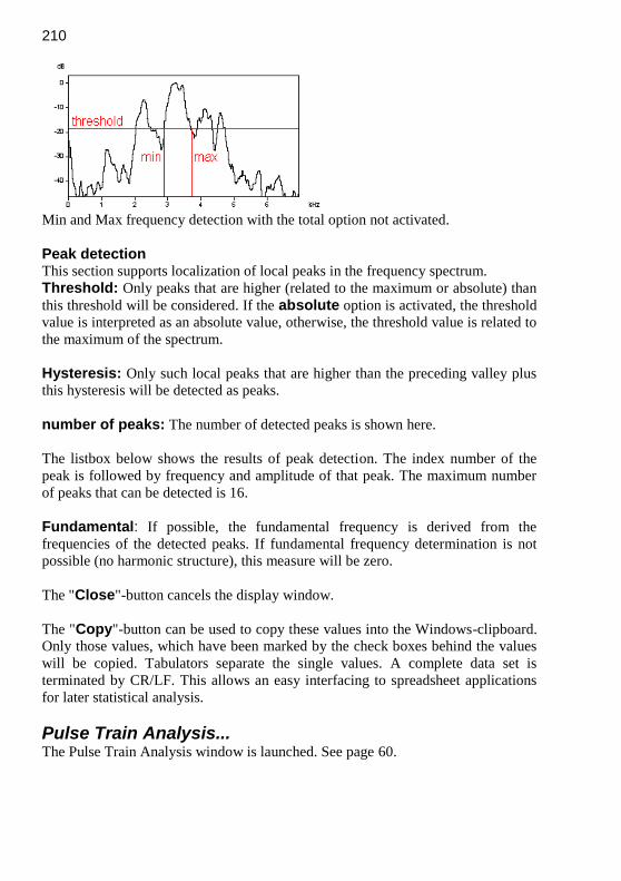
210

Min and Max frequency detection with the total option not activated.

Peak detection This section supports localization of local peaks in the frequency spectrum.

Threshold: Only peaks that are higher (related to the maximum or absolute) than

this threshold will be considered. If the absolute option is activated, the threshold

value is interpreted as an absolute value, otherwise, the threshold value is related to

the maximum of the spectrum.

Hysteresis: Only such local peaks that are higher than the preceding valley plus

this hysteresis will be detected as peaks.

number of peaks: The number of detected peaks is shown here.

The listbox below shows the results of peak detection. The index number of the

peak is followed by frequency and amplitude of that peak. The maximum number

of peaks that can be detected is 16.

Fundamental: If possible, the fundamental frequency is derived from the

frequencies of the detected peaks. If fundamental frequency determination is not

possible (no harmonic structure), this measure will be zero.

The "Close"-button cancels the display window.

The "Copy"-button can be used to copy these values into the Windows-clipboard.

Only those values, which have been marked by the check boxes behind the values

will be copied. Tabulators separate the single values. A complete data set is

terminated by CR/LF. This allows an easy interfacing to spreadsheet applications

for later statistical analysis.

Pulse Train Analysis... The Pulse Train Analysis window is launched. See page 60.

211

Tools

Insert bound cursor Inserts a vertical measuring cursor that moves along the curve. Two of these can be

activated in order to measure differences.

Insert free horizontal cursor Inserts a free moveable horizontal measuring cursor. Two of these can be activated

in order to measure differences.

Remove cursor Removes the measuring cursors.

Harmonic cursor When this option is checked, the measuring cursors will have a harmonic style. In

that mode of operation, the cursor also shows multiples of the fundamental cursor

frequency. This supports measuring the fundamental frequencies of complex

harmonic sounds. Each of the cursor harmonics can be dragged by mouse, which

allows precise fundamental frequency measurements.

The following three label commands are only available for displays versus

time [s].

Cursor linkage between Instances… This dialog allows to define cursor linkages between different instances of the

SASLab Pro software. See page 157 for details.

Insert label See page 162.

Insert section label See page 162.

Label settings... See page 162.

Generate section labels This command will generate section labels from the current gate function

measurements. This command is only available for the “Gate function

(signal/silence duration)”.

212

Keyboard Shortcuts and Popup Menu This command allows defining the keyboard shortcuts for all menu commands of

the selected window. Additionally, each command can be added to the popup

menu, which is activated by right clicking on the window. To modify a keyboard

shortcut, first select the command on the list and then activate the desired shortcut

on the bottom of the dialog box. In order to simplify the access to frequently used

commands, it is recommended to use appropriate shortcuts or popup menu entries

for these commands.

Edit

Smooth The data record is averaged (moving average). The number of consecutive samples

specified in the Average over list box are accumulated and divided by that number.

The corresponding bandwidth of the averaging process is displayed under

corresponds to.

Power spectrum If the displayed data record is an amplitude spectrum, it can be converted into a

power spectrum by this menu option.

Normalize to maximum The displayed data record is normalized to its maximum. The maximum is scaled

to 1 Volt. If the data record is a power spectrum the maximum is scaled to 0 dB.

For measuring the data record, two reticule cursors can be activated. This is done

by clicking into the region at the left of the Y-axis followed by dragging the mouse

cursor to the desired X-position of the data record.

213

The Real Time Spectrograph Window

The real time spectrograph allows Spectrogram display during recording. The

recorded signals delivered by the tape recorder are visualized simultaneously to

human perception on the screen. This window can be activated from the main

window command File/Real Time Spectrogram

The Real time display is started by the menu "Record"/"Start" or the button

. The real time display can be stopped by the menu "Record"/"Stop" or by the

button . The menu "Record"/Pause" or the button can be used to

interrupt the real time display.

Simultaneous to the display of the spectrogram the last recorded time data are

stored in a special data buffer. The buffer size can be adjusted under the menu

"Parameter"/"Buffer Size" . In case of recognizing an interesting sequence the data

stored inside the buffer can be transferred to the main window with the menu

"Record"/"Transfer to Main Window" or the button . These data are displayed

immediately inside the main window. This function allows easy selection of

interesting sequences from long tape recordings for spectrographic analysis.

214

The menu "Parameter"/"Spectrogram-Parameter..." or the button allows

adjusting of Spectrogram-Parameters for real-time display. The display contrast

can also be adjusted by the buttons and .

The window size can be adjusted in order to obtain an optimal screen usage.

For save detection of over-modulation, the button will turn into , once an

over-modulation is detected. Press that button to reset the over-modulation status

flag.

Frequency and time measurements can be made using the cross cursor on the

spectrogram image. For measuring durations click at the start point and drag the

mouse cursor to the end point. The associated results will be displayed at the top of

the window. If you cannot see the results, enlarge the horizontal size of the

window.

File Transfer buffer into main window (and optionally save into file): The

content of the buffer is transferred into the main window.

Save into numbered .wav file and increment : If this option is activated, the

content of the buffer will be saved into a self-incrementing numbered .wav file

each time, the “Transfer buffer…” command is executed. The files will be written

into the Avisoft program directory. The file number can be reset from the menu

Record/Automatic Recording/Reset. Before resetting, the existing files should be

renamed or moved to another folder to prevent overwriting.

Print Spectrogram: The content of the data buffer (not only the visible signal) is

printed.

Save Spectrogram: The content of the data buffer (not only the visible signal) is

saved in a graphics file.

Copy Spectrogram: The content of the data buffer (not only the visible signal)

is copied to the clipboard in spectrographic representation.

Record Start: Starts real-time spectrogram display.

Stream into WAV file: If this option is activated, all sound data displayed in the

real-time spectrograph window will continuously be written into a WAV file. At

the beginning of each recording session (when the record button is pressed) a

SaveAs dialog box is launched to define the file name under which the data will be

saved.

Auto start mode: If this option is activated, recording is started each time the

real-time spectrograph is launched.

215

Start (read from file): Starts real time display with data taken from a *.wav file.

The sound will be played back through the soundcard while the spectrogram is

displayed. A File-Open dialog will be launched when this menu option was chosen.

Alternatively, this display mode can be started by dragging a *.wav-file from the

file-manager into the real-time spectrogram window.

Stop: Cancels real-time display.

Pause: Interrupts real-time display.

Automatic Recording... During real-time spectrogram display it is possible to save acoustic events

automatically. Automatic recording is a triggered data acquisition. Each time the

input signal exceeds a predefined threshold within a given frequency domain, a

new T*.WAV file is generated, and the input signal will be stored for a predefined

hold time in that file. If the threshold is exceeded again within that hold time, the

recording will be extended until there is no further threshold exceeding detected.

This technique ensures, that only one single file is generated from one complex

acoustic event, even if there are short silent sections in it. Alternatively, all events

can be stored into a single .wav file.

This dialogue box allows setting the parameters for this mode of operation.

Automatic event recording into .wav file This check box enables the automatic recording mode. Even if this option is

disabled, the trigger status (“TRG”) will be displayed on the top of the real-time

spectrogram window, which is useful for the adjustment of the trigger.

Autotransfer event waveform If this option is activated, each detected event is transferred automatically into the

main window. This option supports real-time classification, if additionally the main

window option Actions/On new sound file/Create spectrogram is activated.

Autotransfer event spectrogram If this option is activated, each detected event is transferred automatically into the

spectrogram window (as a spectrogram only). This option supports real-time

classification. In contrast to the above option Autotransfer event waveform, the

spectrogram option does not require to recalculate the spectrogram, which may

accelerate the classification process.

Enable automatic recording

This check box enables the automatic recording mode. Even if this option is

disabled, the trigger status (”TRG”) will be displayed on the top of the real-time

spectrogram window, which is useful for the adjustment of the trigger.

216

Automatic Response Setup.. See page 195.

Reset overflow flag Use this command to reset the overflow flag.

Freeze display (toggle)

This command freezes the current display for observation. The recording process

will not be affected. This command should be executed by a keyboard shortcut

(Esc) in order not to delete the current display. Executing this command again will

continue the running display.

Trigger Threshold The threshold for triggering is expected in percent of the measurement range (full

scale). Low values will make the system more sensitive for soft signals. The

threshold should be selected carefully. If that value is too small, you will get a lot

of undesired recordings caused by other soft disturbances. If the value is too large,

you may loose recordings you are interested in because the signal level was below

the threshold. To adjust the threshold, you should try different settings while

automatic recording is disabled. A recognized trigger event is indicated by the

string ”TRG” on the top of the real-time spectrogram window.

Frequency domain The comparison with the threshold is done only with that part of the input signal,

which is within the specified frequency domain. This frequency selectivity helps to

distinguish between the signals you are interested in and other disturbances. Please

note, that the internal frequency resolution is derived from the FFT length of the

spectrogram display. In other words, only frequency differences visible on the

spectrogram can be distinguished by the trigger.

Hold time Each time the threshold is exceeded, a file with at least that duration (hold time)

will be generated. If a new trigger event occurs within that hold time, the recording

will be continued until there is no further trigger event detected. The hold time

should be set as small as possible in order to keep the recording files short.

Minimum duration In order to prevent saving of undesired short events (spikes), the minimum

duration of a trigger event can be specified here. In case the event is shorter than

this value, the file is skipped and will be overwritten by the next one (The file

217

number will not be incremented after closing the file.). The default value is zero,

which means that all events, even the shortest, will be saved.

File name The file name of the next recording file is displayed here. The file name consists of

a leading ”T” followed by a serial number and the extension *.WAV. The serial

number is incremented after each recording. If the option Save all events into a

single file is activated, this edit field allows editing the .wav file name for storing

the events.

The files will be saved into the directory, which was used for the last save

operation (by default the Avisoft directory).

Reset This button resets the internal file counter to one. The name of the next file will

then be T0001.WAV. As a result the old files will be overwritten.

Save all events into a single file If this option is activated, the events will be stored into a single .wav file (instead

of saving into numbered files). The file name under which the events will be saved

has to be specified in the edit field File name. Each new event will be appended to

the existing file. The option Insert break marks will insert a short full-scale pulse

into the .wav file after each event. This allows identifying the single events in later

analysis.

Buffer Size... This dialog box allows determination of the "Buffer size" for saving of most recent

recorded data. The size is expected in kBytes. The buffer size determines the

duration of recorded data depending on the sampling frequency and the data format

(8 or 16 bit, mono or stereo). You should select a buffer size that is as small as

possible for analyzing of data. This will prevent memory conflicts with other

applications.

The "Refreshing time" determines how often the real-time spectrogram display is

updated. This value is expected in percent of the default time. Small values will

give more frequent updates of the display. Depending on the performance of your

computer you can select smaller values. Doing so may raise the risk to lose

samples. So you should try the best value for your computer configuration that

allows recording without gaps.

The option "Enable USG DI trigger" activates the digital input of the Avisoft-

UltraSoundGate for transferring the buffer contents into the main window. If

activated, an active-low signal at the DI will execute the command Transfer buffer

into Main Window. This option should not be activated when using other

218

soundcards than the Avisoft-UltraSoundGate. Doing so would sporadically activate

that command.

With the option "Enable Joystick button #1 / USG button" activated, the buffer

contents will be transferred into the main window by pressing button #1 of a

joystick (or the TRIGGER button an a UltraSoundGate device).

The Default button sets the default values for these parameters.

Envelope If this option is active, the envelope of the signal will be displayed above the

spectrogram. Note that this can slow down the display speed. The color of the

envelope turns to red if the soundcard is over-modulated. In this case you should

reduce the recording level to prevent distortion of the recorded signal.

Scroll-Mode The Spectrogram will be scrolled from right to left in the single-line Spectrogram

display if this option is checked.

Sound Card Settings... See page 28.

Additionally a temporal overlap between 0 and 87.5 % is available. Sound card

sampling frequency and down-sampling is also available from this dialog box. The

down-sampling option allows to further decrease the sampling rates supplied by

the soundcard. That may be useful for the analysis of low frequency signals.

Export-Parameters... See page 136.

Keyboard Shortcuts and Popup Menu This command allows defining the keyboard shortcuts for all menu commands of

the selected window. Additionally, each command can be added to the popup

menu, which is activated by right clicking on the window. To modify a keyboard

shortcut, first select the command on the list and then activate the desired shortcut

on the bottom of the dialog box. In order to simplify the access to frequently used

commands, it is recommended to use appropriate shortcuts or popup menu entries

for these commands.

219

Synthesizer (dialog-based)

The dialogue-oriented synthesizer is suited for the generation of simple single

sound elements. A large number of parameters can be edited numerically. The

parameters are divided into two categories: frequency and amplitude.

Frequency / FM f0 (Fundamental frequency) This is the start frequency at the beginning of the

element.

df (Frequency change) Amount of frequency change over the entire element

duration. If a constant frequency signal is desired, this parameter must be set to 0

Hz.

f(t) (Frequency evolution) Shape of the frequency change df over the entire

element duration dt. The following shapes are available:

Linear: f = f0+df*t/dt

220

Square: f = f0+df*(t/dt)

square2: f = f0+df*(1-(1-t/dt) )

cosine: f = f0+df*cos(t/dt)

sine: f = f0+df*sin(t/dt)

File: f = .ft ASCII file (1 column: time, 2 column:

frequency in Hz or kHz)

If the option "File" is selected, the frequency evolution is taken from the ASCII-

file (*.ft) selected in the list box "user-defined frequency evolution". In this

case the entries f0 and df will be ignored.

Frequency modulation In this section a frequency modulation can be specified.

The following options are possible:

none (no frequency modulation),

Sine (sine shaped frequency modulation),

Triangle. (triangular shaped frequency modulation)

fm (Modulation frequency) At height modulation frequencies this value

corresponds to the distance between the sidebands resulting from FM. At low

modulation frequencies the inverse of this value corresponds to the period time of

the frequency change visible in the spectrogram display.

phi (Phase of the modulation signal) This value determines the first value of the FM. It has only at low modulation frequencies a significant effect. df (Modulation bandwidth) This parameter determines the amount of the

frequency change.

Amplitude / AM A (Amplitude, volume) Absolute amplitude of the fundamental frequency in

Volts (1V corresponds to full scale)

O (Offset) Offset voltage, which is added to the sine signal. (1V corresponds to

full scale)

0.5 1.0 1.5 2.0 2.5 3.0 3.5 4.0 4.5 s

2468

10

kHz

linear square

square2

cosinesine

221

User-defined envelope (a,t-ASCII-file) The selected file (*.at) is used to

generate the amplitude (envelope) of the synthesized signal. t on/off () Duration of fade-in and fade-out at the begin and end of the element.

Fading prevents perceptible noise when the sine generator is switched on or off.

The list box behind allows selecting the shape of fading: linear, sine 1/2 (1/2 sine

period) and sine 1/4 (1/4 sine period).

A0 Relative amplitude of the fundamental frequency compared to the absolute

amplitude of the fundamental A in dB

A1 Relative amplitude of the first harmonic compared to the absolute amplitude of

the fundamental A in dB A2 Relative amplitude of the second harmonic compared to the absolute amplitude

of the fundamental A in dB A7 Relative amplitude of the seventh harmonic compared to the absolute

amplitude of the fundamental A in dB

0 dB means that the harmonics has the amplitude defined in A. -20 dB will

generate a harmonic with 1/10th of the amplitude defined in A. Those harmonics

that are not desired must have a value below -96dB. Alternatively the edit field can

be cleared. If a true sine signal without harmonics is desired, all edit fields from A1

to A7 must be empty and A0 should be set to 0dB.

Amplitude modulation This section allows specifying an amplitude modulation. The following options are

available:

none,

Amplitude: Normal amplitude modulation with conservation of the carrier

frequency (fundamental).

Ring: special amplitude modulation with rejection of the carrier frequency

(fundamental).

fm (Modulation frequency) The modulation frequency corresponds to the distance of the sidebands from the

fundamental frequency.

m (Modulation depth) 0% is no AM, 100% is maximum AM. dt (Tone duration) This is the duration of the signal to be synthesized. The preset value represents the

duration of the marker in the main window.

222

noise Adds white noise with the specified amplitude to the signal (1V corresponds to full

scale). Set this value to zero if no noise is desired. If pure noise is required set the

amplitude of the sine generator (A in section Amplitude /AM) to zero.

Default This button resets all parameters. As a result a pure 1 kHz sine signal at 0.5 V is

entered.

Insert The signal is synthesized and is copied into the main window at the current insert

point.

Clipboard

The signal is synthesized and is copied into the clipboard.

Sampling rate settings… This dialog box allows defining the sampling rate of newly created sound files. The

option ‘in the Sound Card Settings’ will take the currently selected sampling

frequency from the main window menu File/’Sound Card Settings…’. The

alternative option ‘here’ will take the sampling frequency specified in the combo

box behind. Note that the sampling rate settings will only be applied if there is

currently no sound file loaded. Use the main window command File/Close to close

the currently loaded file.

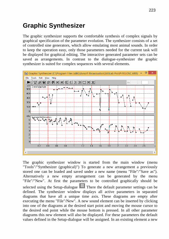
223

Graphic Synthesizer

The graphic synthesizer supports the comfortable synthesis of complex signals by

graphical specification of the parameter evolution. The synthesizer consists of a set

of controlled sine generators, which allow emulating most animal sounds. In order

to keep the operation easy, only those parameters needed for the current task will

be displayed for graphical editing. The interactive generated parameter sets can be

saved as arrangements. In contrast to the dialogue-synthesizer the graphic

synthesizer is suited for complex sequences with several elements.

The graphic synthesizer window is started from the main window (menu

"Tools"/"Synthesizer (graphical)") To generate a new arrangement a previously

stored one can be loaded and saved under a new name (menu "File"/"Save as").

Alternatively a new empty arrangement can be generated by the menu

"File"/"New". At first the parameters to be controlled graphically should be

selected using the Setup-dialogue There the default parameter settings can be

defined. The synthesizer window displays all active parameters in separated

diagrams that have all a unique time axis. These diagrams are empty after

executing the menu "File"/New". A new sound element can be inserted by clicking

into one of the diagrams at the desired start point and moving the mouse cursor to

the desired end point while the mouse bottom is pressed. In all other parameter

diagrams this new element will also be displayed. For these parameters the default

values defined in the Setup-dialogue will be assigned. In an existing element a new

224

point can be inserted by clicking at the element. Existing points can be moved by

the mouse. Entire elements can be moved by the mouse while the Shift key is

pressed. Single points can also by edited numerically. To do this the reticule

marker must be positioned onto the point to be edited. This can be done by mouse

or by using the menu options (Next element , Next point , Previous point

, Previous element ) The edit-fields are located on the top of the window.

The editing commands (menu Edit) allow editing several elements at once. A

section marker can be activated by left-clicking while the Shift key is pressed. This

marker allows to move the selected elements (while the Shift key is pressed). The

Edit commands will work on the selected sections. The current marker can

temporarily be disabled for editing the elements behind the marker (Edit/Disable

marker).

For accurate drawing it is possible to zoom into the graphs ( or menu

"Tools"/"Zoom" and "Tools"/"View..." or by double clicking on the Y-axis). These

techniques are very similar to other graphics applications.

The current state of the arrangement can by played back anytime by the menu

"File"/Play" . The synthesized arrangement can be inserted into the main

window using the menu "File"/"Insert". .

File

New A new (empty) arrangement is generated.

Open... A previously saved arrangement file (.ARR) is loaded. Alternatively, .ARR files

can also be opened by drag & drop into either the SASLab Pro main window or

into the Graphic Synthesizer window.

Save The current arrangement is saved under the current name.

225

Save as... The current arrangement is saved under a new name. The arrangement is saved in

several files. The main file *.arr contains general information on the parameters

used. Depending on the active parameters additional ASCII-files containing the

data points are written. Each of these files consists of two columns. The first

column represents the time in seconds, the second one represents the Y-values of

the parameters in Hz, V, dB or %. These ASCII-files can be easily imported into

spreadsheet applications (Excel) The extensions of the files depends on the type of

parameter (ft, at, a1t, a2t, ... , a7t, fmt, fht, amt, aht; see Setup)

Setup This dialogue allows selecting the active parameters to be edited graphically. The

preset values of the parameters can be entered. Additionally the fadein and fadeout

parameters can be chosen.

In this dialogue all synthesizer parameters are listed. The checkboxes on the left

determine, whether the parameter should appear in the synthesizer window for

graphical editing or not. The edit fields behind the parameter name allow

specifying the preset values of each parameter. This value is taken when a new

element is inserted, regardless whether the parameter is activated for graphical

editing (checked) or not.

The synthesizer consists of three components: sine, noise and pulse train generator.

Sine generator Fundamental frequency Fundamental frequency in Hertz (Extension of the ASCII-parameter-file: ".ft")

Overall Amplitude Absolute overall amplitude in Volts. (full scale: 1V) (Extension of the ASCII-

parameter-file: ".at")

Relative amplitudes of harmonics [dB] This section allows to activate and enter the default relative amplitudes of the

fundamental and the harmonics. The amplitude values are expected in dB

referenced to the Overall amplitude. The extensions of the ASCII-parameter-

files are ".a0t” for the fundamental (F0), ".a1t" for the second harmonic, ".a2t" for

the third harmonic and so on.

226

FM-frequency Frequency-modulation frequency (Extension of the ASCII-parameter-file: ".fmt")

Frequency change of FM Amount of frequency change. This parameter must be set to 0 Hz if no FM is

desired. (Extension of the ASCII-parameter-file: ".fht")

AM-Frequency Amplitude-modulation frequency (Extension of the ASCII-parameter-file: ".amt")

Modulation depth of AM Amount of amplitude modulation. This parameter must be set to 0% if no AM is

desired. (Extension of the ASCII-parameter-file: ".aht")

t on/off Duration of fade-in and fade-out at the start and end of each element. Fading

prevents perceptible noise when the sine generator is switched on or off. The list

box behind allows selecting the shape of fading: linear, sine 1/2 (1/2 sine period)

and sine 1/4 (1/4 sine period).

Averaging time for parameter smoothing The time interval specified here determines the duration of a linear (FIR) filter that

is applied to all parameter curves before the signal is finally synthesized, which

will allows to produce more natural synthetic signals. A time interval of 0 s will

completely inhibit this kind of smoothing. The maximum interval that can be

realized is 1024 samples.

Anti-aliasing filtering If this option is checked, signal components above the Nyquist frequency (half of

the sample rate) will be rejected.

Noise generator The noise generator produces amplitude-modulated white noise signals.

Noise amplitude Amplitude of additional white noise in Volts. (full scale: 1V) (Extension of the

ASCII-parameter-file: ".nt") This noise generator is independent from the sine

generator. In other words, the parameters of the sine generator as Overall

Amplitude and t on/off will not influence the noise generator. If only noise without

harmonic components is desired, set the Overall Amplitude of the sine generator to

zero.

227

Pulse train generator The pulse train generator supports the generation of amplitude modulated pulse

trains with pulse rates varying over time. The single pulse is supplied as a .wav file

in 16-bit mono format. This pulse train generator is independent from the sine and

noise generator. In other words, the parameters of the sine generator as Overall

Amplitude and t on/off will not influence the noise generator. If only pulse train

generation is desired, set the Overall Amplitude of the sine generator and the Noise

amplitude of the noise generator to zero.

Pulse train amplitude envelope Amplitude of the pulse train (full scale: 1V) (Extension of the ASCII-parameter-

file: ".pta")

Pulse rate Pulse rate in Hz (Extension of the ASCII-parameter-file: ".ptr"). The pulse rate is

limited by the duration of the pulse file. The maximum overlap between

consecutive pulses is 93.75%. Exceeding this overlap will produce unpredictable

results. So the maximum pulse rate is fp=16/pulse_duration (fp in Hz and pulse

duration in seconds).

Pulse file... This button launches a dialog box to select the .wav file containing the pulse to be

used in pulse train synthesis. That .wav file must be in 16 bit mono format.

Default This button resets all parameter entries.

Play The current arrangement is synthesized and played back through the soundcard.

Insert The current arrangement will be synthesized and inserted into the main window.

Insertion takes place at the current insertion position (left margin of the marker).

Insert into clipboard The current arrangement will be synthesized and copied into the clipboard.

228

Save into WAV file The current arrangement will be synthesized and saved into a WAV file. The

sampling rate for this file can be set from File/Sampling rate settings…

Sampling rate settings… This dialog box allows defining the sampling rate of newly generated sound files.

The option ‘in the Sound Card Settings’ will take the currently selected sampling

frequency from the main window menu File/’Sound Card Settings…’. The

alternative option ‘here’ will take the sampling frequency specified in the combo

box behind.

Open last arrangement on start If this option is activated, the previous arrangement used at the last session will be

loaded each time the Graphic Synthesizer is started.

Tools

Zoom A rectangular section of the current view will be magnified. The mouse cursor

changes into an up-arrow that allows selecting the desired section.

Unzoom The entire signal is displayed.

Unzoom with zero The entire signal including the zero line is displayed.

View The visible section of whole signal is adjusted manually.

Grid A grid is inserted or removed.

Next element The marker is moved to the next element.

Next point The marker is moved to the next point.

229

Previous point The marker is moved to the previous point.

Previous element The marker is moved to the previous element.

Delete point The marked point will be deleted. Alternatively, a point can be deleted by right-

clicking at the point and selecting the appearing popup menu entry.

Delete element The marked element will be deleted. Alternatively, an element can be deleted by

right-clicking at the element and selecting the appearing popup menu entry.

Lock time-axis Disables editing of the time coordinates. This option should be activated, if the Y-

coordinates of an existing element have to be edited, while the time-coordinates

must be maintained.

Lock Y-axis Disables editing of the Y-coordinates. This option should be activated, if the time-

coordinates of an existing element have to be edited, while the Y-coordinates must

be maintained (time-shifting of elements).

Scan harmonics from spectrogram based on fundamental

The amplitudes of the harmonics are extracted from the spectrogram that is visible

in the Spectrogram window (use the option View/Display spectrogram to show

that spectrogram). The fundamental frequency curve must have been specified

before by manual drawing in the Fundamental frequency section or by the Scan frequency contour spectrogram function. If the signal to be scanned has many

harmonics it may be useful to manually trace a higher harmonic instead of the

fundamental itself. The menu option Scaling can then be used to multiply the

frequency scale by a factor (e.g. 0.25 if the 4th harmonic was traced) in order to get

more precise fundamental frequencies.

230

The accuracy of the scanning procedure is influenced by the quality of the

spectrogram, it’s resolution and the precision of the fundamental frequency curve

supplied. The precision of the fundamental frequency curve is especially important

for high order harmonics. For scanning the 7th harmonic, the specified

fundamental frequency is multiplied by 7 and the amplitude at that frequency

position in the spectrogram is taken as the amplitude of the 7th harmonic.

number of harmonics to scan: This list box determines the number of

harmonics, which will be traced. This value can be any integer between 0 and 7.

Zero means, that only the fundamental itself is scanned.

max. deviation A(t): This value determines the accuracy of the amplitude trace.

It is expressed in percent of the maximum magnitude of the entire spectrogram.

Larger values will produce fewer samples in the amplitude plot, which may

simplify any further editing of the elements. In order to get maximum fidelity it is

recommended to set this value to zero.

Scaling

This option allows to rescale the time and y parameters of the current arrangement.

Time and y parameters can be adjusted independently. Additionally, it is possible

to completely remove the modulation (e.g. AM or FM) from single parameters. If a

section marker has been activated, only the selected elements will be modified.

multiply time axis by The time scale of all parameters is multiplied by this

factor. Values greater than one will stretch the entire arrangement in time. Values

between zero and one will compress the time axis.

Parameter (y axis) This listbox allows to choose the y parameter to be modified.

multiply by The selected parameter is multiplied by this factor (applies to all

elements).

add This value (unit Hz, V or dB) is added to the selected parameter (applies to all

elements). This value can be positive or negative.

normalize The selected parameter is normalized in such a way that its maximum

value is set to the specified value. In case the overall option is not checked, the

normalization will be done individually for each element.

remove modulation The modulation present in the selected parameter will be

removed from each element. The resulting constant parameter will represent the

average of the original (modulated) parameter within each element.

231

Single elements can be modified separately by right-clicking at the desired

parameter of an element and selecting the popup menu item “Element Scaling”.

Copy contour…

The copy contour command allows to copy the contour of one parameter to

another. For instance, it would be possible to move the course of the overall

amplitude to the noise amplitude in order to create a synthetic noise signal that has

the same amplitude modulation contour as previously scanned natural whistle.

Edit

The Edit commands allow moving or manipulating several elements at once. The

elements to be processed have first to be selected by using the section marker. That

marker can be activated by left-clicking while the Shift key is pressed. The time

coordinates and the duration of this marker is displayed on the top of the

Synthesizer window.

Copy Copies the selected elements into an internal clipboard.

Paste Inserts the content of the clipboard at the selected position.

Cut Cuts the selected elements and copies them into the clipboard.

Delete Deletes the selected elements without moving the following elements.

Append Appends the content of the clipboard behind the last element.

Remove marker Removes the marker.

232

Disable marker This option temporarily disables the current marker. If this option is activated, the

elements hidden by the marker can be edited while the position of the marker is

still visible (for orientation).

View

Display Spectrogram If this option is checked, the spectrogram of the Spectrogram window will be

displayed as a background image. This can be useful when the synthetic signal

should be derived from the spectrographic representation of a natural signal.

Display Instantaneous frequency / Zero crossing analysis If this option is checked, the instantaneous frequency (or zero crossing analysis)

plot from the One-dimensional Transformation window will be displayed as a

background image. This can be useful when the synthetic signal should be derived

from the frequency course of a natural signal.

Fundamental Frequency, Overall Amplitude, Rel. amplitude, ... In this menu section all active parameters are listed. Those parameters visible in

the synthesizer window are checked. Each parameter can temporarily hidden by

un-checking the parameter in order to get more space for the other parameters.

Alternatively, the parameters can be hidden by clicking on the parameter title on

the graphs.

233

Example of AM The example below shows the spectrogram of a synthesized signal with AM-

frequency sweeping from 10 to 1000Hz. All other parameters are constant

(Fundamental frequency = 5kHz, Modulation depth of AM = 100%)

Example of FM The example below shows the spectrogram of a synthesized signal with FM-

frequency sweeping from 10 to 1000Hz. All other parameters are constant

(Fundamental frequency = 5kHz, Frequency change of FM = 3kHz)

234

Guidelines for making correct spectrograms

Over-modulation

Take care that the record level of the sound card

is adjusted correctly. If the signal exceeds the

dynamic range of the sound card, signal

distortion will occur. This over-modulation is

audible while playing back the recorded signal.

On the spectrogram additional harmonic

frequency components that are not part of the

original signal can be seen.

Note that over-modulation can also happen

during recording the sounds with your tape

recorder.

Aliasing

A basic demand in digital signal processing is, that the sampling frequency must be

at least twice the maximal frequency of the signal to be sampled. Most sound-cards

have an onboard anti-aliasing filter (due to the type of analog-to-digital converter,

which is usually a Sigma-Delta type) that suppresses all signal frequencies above

one half of the sampling frequency. If there is no anti-aliasing filter all signal

frequencies above one half of the sampling frequency will be transformed to lower

frequencies. In

A sine sweep signal from 1 to 9 kHz sampled with 16 kHz.

The end of sweep with 9 kHz occurs at 7 kHz in the spectrogram!

235

The Avisoft-CORRELATOR

The Avisoft-CORRELATOR supports the

computation of sound-similarity-matrixes of

spectrograms made by the Avisoft-SASLab Pro.

This enables you to check the similarities of

several spectrograms. All selected spectrograms

are compared each other. Each comparison is

done by sliding the two spectrograms past each

other along the time axis. An additional sliding in

frequency can be specified if small frequency

deviations of the signals should be ignored. The

correlation coefficients are computed for all time-

(and frequency-) offsets. The peak value of the correlation coefficients is saved in a

correlation matrix. Another application of the CORRELATOR is time and

frequency aligned averaging of spectrograms.

How to use the Avisoft-CORRELATOR The Avisoft-CORRELATOR is a separate application that is installed along with

the SASLab Pro software. It can be found at All apps > Avisoft Bioacoustics > Avisoft-CORRELATOR. The executable file corr32.exe is located in the folder

C:/Program Files (x86)/Avisoft Bioacoustics/SASLab Pro.

The spectrograms have to be saved in ASCII or Binary format using the

"File"/”Data Export”/"Save ASCII/Binary Spectrogram" option of the Avisoft-

SASLab spectrogram window. The ASCII-files must be saved with the extension

".txt". Binary spectrograms must have the extension .SON. All spectrograms to be

correlated should have the same sampling frequency and the same spectrogram

parameters. All spectrograms must be saved in a unique path.

After finishing the ASCII/Binary spectrogram

generation in Avisoft-SASLab Pro, you can start

the Avisoft-CORRELATOR. The following

steps have to be done:

Select the files to be compared First you have to specify the spectrogram files to

be correlated. This is done by the menu

‘File’/’Select...’.

236

In the edit box ‘Path:’ it is required to specify the path, where the spectrogram (or

waveforms, envelopes or spectra) files are located. ASCII spectrogram files must

have the extension *.txt. Binary spectrograms should have the extension *.son. The

desired file format (*.TXT or *.SON) must be selected from the File format list

box.

The list box titled Type of data allows to select the type of data that should be

correlated:

Spectrograms (.son, .txt) (default)

Waveforms or Envelopes (.wav for .txt)

Spectra (.txt)

The files that should be correlated must be selected from the

By clicking on the files listed in the file listbox you can select. Press the button

‘OK’ when you have finished the selection. As a result of the file selection an

empty similarity-matrix will be displayed.

Start the correlation process / Defining the correlation parameters

Then you can start the correlation process by the

menu "Analyze/"Start...". After the software has

tested the selected files the "Correlation-

Parameters" dialog box is displayed.

Here you have to specify the sampling frequency

of the sound files the spectrograms have been created from, because this

information is not part of the ASCII-spectrogram-files.

In order to remove low frequency disturbance signals, which would distort the

correlation coefficients, you can specify the desired cut-off-frequency. All

components of the spectrogram below the specified cut-off-frequency will be

ignored.

If the signals to be correlated slightly differ in frequency no similarity would be

found unless a tolerating frequency deviation is specified. In this case the two

spectrograms to be correlated will be slid additionally along the frequency axis in

order to find the true peak similarity. The number of correlation’s necessary to

realize this tolerating behavior is displayed behind the line "resulting number of

correlations". Note that this will cause a multiplication of computing time! After

237

pressing the "OK"-button the similarity matrix is computed. This can take a very

long amount of time depending on the sizes of the spectrograms and the specified

correlation parameters.

You can cancel the correlation process before ending by pressing the "Cancel"-

button at the top of the window.

The correlation can be repeated with the same files and different correlation

parameters by resetting the correlation matrix (menu "Analyze/"Reset") and

starting the correlation again using different parameters (menu "Analyze/"Start...").

Exporting the correlation matrix

The matrix of correlation coefficients displayed on the screen can be copied into

the Windows clipboard by using the command "File"/"Copy Matrix". The matrix

can also be saved (Save Matrix) or printed (Print Matrix). This allows the export of

the matrix into other applications such as spreadsheet or statistical analysis

programs.

Averaging of aligned spectrograms The CORRELATOR can also be used to average several aligned spectrograms.

This is done in two steps:

Calculating the shift between the spectrograms to be averaged.

Averaging of the spectrograms using the previously calculated shifts.

To enable this mode of operation, activate the menu option ‘Analyze’/’Aligning

mode’. Then proceed as described at Selecting the files to be processed. The

command Analyze/Start will then compute the shifts between the selected files.

The correlation coefficient, the X and Y shift (in pixel units) will be displayed for

each file. Then use the command ‘File’/’Average and Save aligned spectrograms’

to execute the averaging. You will be prompted for a file name for the averaged

spectrogram (*.son).

Alternatively the command ‘File’/’Select, Align, Average and Save

spectrograms...’ can be used to execute the entire process at once.

The resulting averaged spectrogram will have the same dimension as the last

spectrogram in the list of selected source spectrograms. Any longer spectrograms

on the list will be cropped to that size.

238

The averaged spectrogram (*.son) can be viewed in Avisoft-SASLab Pro using the

main window command ‘Analyze’/’Open Spectrogram...’ or ‘File’/’Open

Spectrogram...’ from the spectrogram window.

239

The correlation algorithm

The peak correlation coefficient displayed in the correlation matrix is defined as

follows:

The two spectrograms are shifted incrementally past each other along the time axis.

For every offset position the correlation coefficient is computed according to the

following formula:

x x y

bxy

y

axy

x y

bxyaxy

XY

mbma

mbma

22 )(*)(

))(*)((

Where ma and mb are the mean values of the spectrograms. axy and bxy are the

intensities of the spectrogram points at the locations x,y.

The correlation coefficient is a value ranging from -1 to +1. A one means that the

two spectrograms are identical. A zero means that there is no similarity between

the spectrograms. Values below zero occur when the two spectrograms are inverse.

The peak value of the correlation coefficients of all shift-offsets between the two

spectrograms is saved in the correlation matrix.

Discussion of the correlation method

If you use the Avisoft-CORRELATOR you should always keep in mind that the

numerical correlation method used in the Avisoft-CORRELATOR delivers only

correlation coefficients computed by a stupid mathematical algorithm. This

algorithm cannot recognize complicated spectrogram structures like a human could

do it.

For this reason the correlation method is suited for the following kinds of

spectrograms only:

The spectrogram should contain only one syllable. If there would be more than

one syllable, the correlator would recognize similarities only if the distance

between the syllables is exactly identical.

240

The spectrograms should be generated using small FFT lengths or (and) small

frame-sizes to reduce the frequency resolution. High frequency resolution would

prevent good results if there are any differences in frequency of two evidently

similar spectrograms.

In many cases it is recommended to use parametric methods instead of this

correlation method. For the parametric method such parameters as frequency and

duration can be taken from the spectrogram using the measuring cursors or the

Automatic Parameter Measurements facility of Avisoft-SASLab.

241

Tutorial Opening sound files from a CompactFlash or Harddisk recorder

The new CompactFlash and Harddisk recorders (e.g. Marantz PMD670, PMD660,

Fostex FR-2, Edirol R-09, Sound Devices 722) change the way how to transfer

sound recordings into the PC for analysis. Because these recorders already save the

sound recordings as common sound files (.WAV, (*.MP3)), the transfer (upload)

of the recordings is very simple.

Once the recorder has been connected to the PC via its digital interface (either USB

or FireWire), the recorder will appear on the PC as a standard mobile mass storage

device (like any other external harddisk). So, there is no difference whether the

sound files physically reside on the recorder or on the PC. However, in order to

speed-up the sound analysis, it is recommended to copy (upload) the files first onto

the computer harddisk (certainly a slow USB 1.1 interface might be too slow for a

smooth work flow). Besides of this transfer speed issue, the sound file upload is

also strongly recommended for archiving the recordings onto more cost-effective

storage media (CD, DVD, external harddrives).

A separate Card Reader interface would be useful for downloading the data from

the CF cards in case you are using a recorder with a slow USB 1.1 interface.

Avisoft-SASLab Pro provides various ways to open these .WAV files efficiently

(either the original files directly from the recorder or the mirrored files from the

harddisk):

Main Window

Command File/Open...

Command File/Browse...

Drag&Drop from the Windows file

manager window

Command File/Specials/'Next file';

'previous file' (default keyboard shortcuts Strg+N and Strg+P or the

buttons < and >)

242

Spectrogram Window

These commands will load the WAV file and automatically create a spectrogram of

the entire file.

Command WavFile/Open...

Drag&Drop from the Windows file manager window

Command WavFile/'Next file'; 'previous file' (default keyboard shortcuts

Strg+N and Strg+B or the buttons < and >)

Real Time Spectrograph Window

The WAV files opened here will be played back continuously (while the real-time

spectrogram is displayed). So, this option is useful for scanning longer files. Use

the command File/'Transfer buffer into main window' to pick out a sub-section out

of the original large file. The Real Time Spectrograph Window is launched from

the main window command File/'Real Time Spectrogram...'.

Command Record/Start (input from file)...

Drag&Drop from the Windows file manager window

Note that MP3 files are not supported by Avisoft-SASLab Pro due to the potential

artifacts introduced by the lossy compression algorithm. For processing such

compressed files it is necessary to convert them into uncompressed .wav files. This

can be done for instance by using the free Lame/RazorLame decoder.

CompactFlash and Harddisk recorder usually allow to select the sample rate. The

sample rate should be adopted to the frequency range of the sounds that you want

to analyze (the sample rate should be at least about 250 % of the maximum signal

frequency you are interested in). If you are unsure, then you should select a higher

sample rate (at the expense of larger file sizes).

243

Measuring sound parameters from the spectrogram manually

There are several ways to measure sound parameters from the spectrogram:

The ‘Standard marker cursor’ allows

to measure duration’s by left-

clicking and dragging. The

associated values are displayed at

the right top corner of the

spectrogram window. The current

duration value can be exported as an

ASCII string by File/Data

export/Copy measured value or

Copy t1, t1. Alternatively simply

click at the top right cursor value

frame. The ASCII string is copied

into the clipboard and can be pasted

from other applications.

Additionally, the single values can

be automatically transferred into an

Excel spreadsheet. This can be

configured from File/Data

export/’DDE- Parameters / Log

file…’

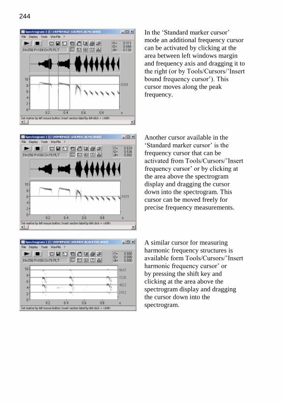
244

In the ‘Standard marker cursor’

mode an additional frequency cursor

can be activated by clicking at the

area between left windows margin

and frequency axis and dragging it to

the right (or by Tools/Cursors/’Insert

bound frequency cursor’). This

cursor moves along the peak

frequency.

Another cursor available in the

‘Standard marker cursor’ is the

frequency cursor that can be

activated from Tools/Cursors/’Insert

frequency cursor’ or by clicking at

the area above the spectrogram

display and dragging the cursor

down into the spectrogram. This

cursor can be moved freely for

precise frequency measurements.

A similar cursor for measuring

harmonic frequency structures is

available form Tools/Cursors/’Insert

harmonic frequency cursor’ or

by pressing the shift key and

clicking at the area above the

spectrogram display and dragging

the cursor down into the

spectrogram.

245

The ‘Free reticule cursor’ is a thread

cross cursor replacing the mouse

cursor. In this mode time, frequency

and amplitude can be measured.

Left-clicking will export the current

values. The ‘Bound reticule cursor’

is the same, except that the

frequency thread moves along the

peak frequency (the current vertical

mouse cursor position is ignored).

The ‘Magic reticule cursor’ allows

to track frequency contours in

complex (harmonic) sounds. With

the option “locate and measure

entire elements” activated, several

sound parameters as duration,

max/min and start/end frequency

can be measured quickly by placing

the mouse cursor over the element

to be analyzed.

246

Labels

Labels can be placed anywhere on

the spectrogram. A short label text

can be annotated to either a single

point at a certain time/frequency

location or to a time section (section

label). Single point labels are

annotated from Tools/Labels/’Insert

labels’. Alternatively, his can be

done right –clicking and selecting

the associated popup menu item.

The coordinates of these labels can

be exported from

Tools/Labels/’Label settings…’ by

the button ‘Copy’. This will copy

the selected labels as an ASCII table

into the clipboard, which can

subsequently be pasted into an Excel

spread sheet for instance.

Section labels can be used to create

a specific grid for logging data at

regular intervals with the ‘Free

reticule cursor’. The cursor then

snaps automatically into the

temporal grid. This grid option can

be activated from

Tools/Labels/’Section labels grid…’

This may be especially useful for

signals where automatic methods

are not possible.

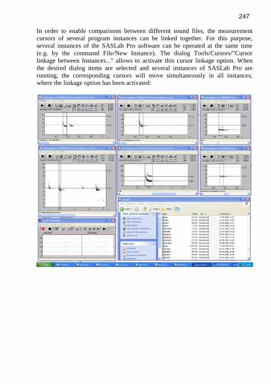
247

In order to enable comparisons between different sound files, the measurement

cursors of several program instances can be linked together. For this purpose,

several instances of the SASLab Pro software can be operated at the same time

(e.g. by the command File/New Instance). The dialog Tools/Cursors/"Cursor

linkage between Instances..." allows to activate this cursor linkage option. When

the desired dialog items are selected and several instances of SASLab Pro are

running, the corresponding cursors will move simultaneously in all instances,

where the linkage option has been activated:

248

Measuring sound parameters from the spectrogram automatically

The success of the automatic measurements will heavily depend on the type of

sounds, the quality of sound recordings and the configuration settings made under

Tools/Automatic parameter measurements/’setup…’. The first and most essential

step in configuring this tool is to establish a safe element separation. There are four

options in the ‘Element separation’ section:

Figure 1: The Automatic Parameter Measurements setup dialog.

automatic (single threshold) Use this option for sound files, where all

elements nearly have the same amplitude.

automatic (two thresholds) This option is suited for sound files containing

elements with varying amplitudes.

automatic (three thresholds) Use this option for sound files containing

elements with varying amplitudes that require separate thresholds for detecting the

start an end of each element

interactively (section labels )This option is appropriate for sounds where the

automatic element separation is not possible.

automatic (whistle tracking) This option is suited for detecting soft whistles in

noisy sound recordings.

249

automatic (single threshold)

The single threshold is used for both detecting the elements and the determination

of the start and end point of each element:

Figure 2a: Single threshold element separation (option "relative to maximum" not

activated).

Figure 2b: Single threshold element separation (option "relative to maximum"

activated).

The point where the amplitude exceeds the threshold is assumed to be the start of

an element. Similarly, the point, where the amplitude goes first below the threshold

is the end point of the element.

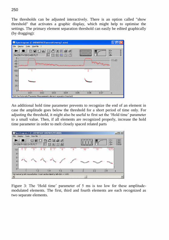
250

The thresholds can be adjusted interactively. There is an option called "show

threshold" that activates a graphic display, which might help to optimise the

settings. The primary element separation threshold can easily be edited graphically

(by dragging):

An additional hold time parameter prevents to recognize the end of an element in

case the amplitude goes below the threshold for a short period of time only. For

adjusting the threshold, it might also be useful to first set the ‘Hold time’ parameter

to a small value. Then, if all elements are recognized properly, increase the hold

time parameter in order to melt closely spaced related parts

Figure 3: The ‘Hold time’ parameter of 5 ms is too low for these amplitude-

modulated elements. The first, third and fourth elements are each recognized as

two separate elements.

251

Figure 4: Increasing the ‘Hold time’ parameter to 50 ms provides satisfying results.

Figure 5: Larger amplitude differences lead to poor start and end point locations. In

such cases use the ‘two thresholds’ option described below.

252

automatic (two thresholds)

The first threshold is used for element detection only. The second start/end

threshold is used to determine start and end points. The specified relative start/end

threshold is used to calculate an internal individual absolute threshold for each

detected element:

Figure 6: Two thresholds element separation: The first absolute threshold for the

element detection is shown as a continuous horizontal line. The short lines depict

the second relative start/end threshold that is referenced to the maximum of each

detected element. In this way, the automatically recognized element borders are

independent from the absolute element amplitudes. This is especially important for

vocalizations with high dynamic ranges (both loud and soft elements) or in

recording situations with varying distances between the animal and microphone

(e.g. flying bats). Adjusting the two parameters should be done in the following

sequence: First use the ‘automatic (single threshold)’ mode to adjust the first

absolute threshold for element detection. Modify this value until all elements are

recognized safely. At this stage it does not matter, whether the element borders are

recognized correctly. It is only important that there is a number displayed above

each element:

Figure 6: Adjusting the absolute element detection threshold. Then switch back to

the ’automatic (two threshold)’ mode to adjust the second relative ‘start/end

253

threshold’. Start with high values (e. g. –5dB) and decrease the relative threshold

(down to – 10 … - 20 dB), depending on the structure of your signals.

Alternatively, adjusting the two thresholds can be done without switching into the

single threshold mode. Then first set the ‘start/end threshold’ to 0 dB to find the

correct absolute element detection threshold.

Figure 8: The relative start/end threshold of –17dB is too low. The reverberation

noise between the elements prevents proper element separation at this low

threshold.

Figure 8: Correctly recognized elements (using a start/end threshold of –11 dB),

despite of the varying element amplitudes.

254

automatic (three thresholds)

This option is similar to the above two thresholds option, except that there are two

separate thresholds for the localization of the start and the end of each element.

This is certainly useful for sounds influenced by reverberation.

255

If there is too much noise that prevents the automatic recognition, you might try to

remove that noise. If the noise does not overlap with the sounds of interest, then a

simple high- or low-pass filter might help. It is possible to hide low frequencies on

the spectrogram window from the command Display/'lower Cut-Off Frequency...'

In case the noise overlaps with the sound elements, then it would be possible to

remove that noise manually by using the command Tools/Cursors/'Standard eraser

cursor':

Figure 10: Noise prevents the proper element detection

Figure 11: Manually erasing the noise provides the desired result

Another option for rejecting broad-band noise is the Entropy option in the 'Post

filter' section. The whistle tracking option described later might also help to handle

noisy recordings.

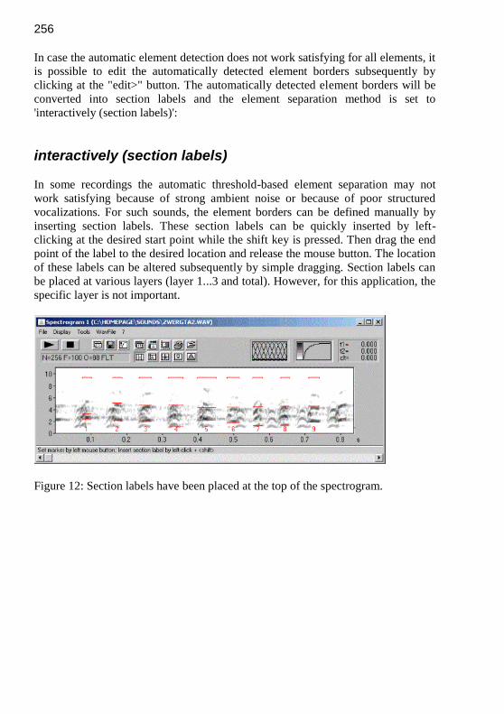
256

In case the automatic element detection does not work satisfying for all elements, it

is possible to edit the automatically detected element borders subsequently by

clicking at the "edit>" button. The automatically detected element borders will be

converted into section labels and the element separation method is set to

'interactively (section labels)':

interactively (section labels)

In some recordings the automatic threshold-based element separation may not

work satisfying because of strong ambient noise or because of poor structured

vocalizations. For such sounds, the element borders can be defined manually by

inserting section labels. These section labels can be quickly inserted by left-

clicking at the desired start point while the shift key is pressed. Then drag the end

point of the label to the desired location and release the mouse button. The location

of these labels can be altered subsequently by simple dragging. Section labels can

be placed at various layers (layer 1...3 and total). However, for this application, the

specific layer is not important.

Figure 12: Section labels have been placed at the top of the spectrogram.

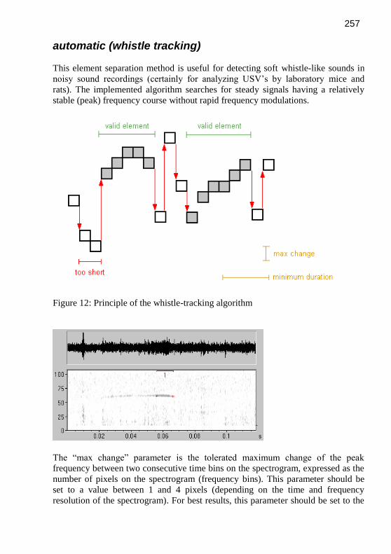
257

automatic (whistle tracking)

This element separation method is useful for detecting soft whistle-like sounds in

noisy sound recordings (certainly for analyzing USV’s by laboratory mice and

rats). The implemented algorithm searches for steady signals having a relatively

stable (peak) frequency course without rapid frequency modulations.

Figure 12: Principle of the whistle-tracking algorithm

The “max change” parameter is the tolerated maximum change of the peak

frequency between two consecutive time bins on the spectrogram, expressed as the

number of pixels on the spectrogram (frequency bins). This parameter should be

set to a value between 1 and 4 pixels (depending on the time and frequency

resolution of the spectrogram). For best results, this parameter should be set to the

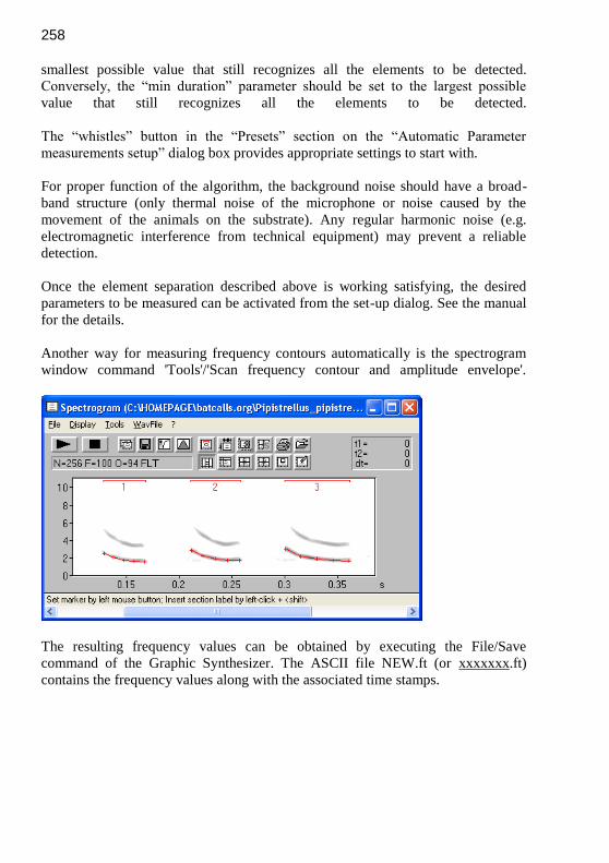
258

smallest possible value that still recognizes all the elements to be detected.

Conversely, the “min duration” parameter should be set to the largest possible

value that still recognizes all the elements to be detected.

The “whistles” button in the “Presets” section on the “Automatic Parameter

measurements setup” dialog box provides appropriate settings to start with.

For proper function of the algorithm, the background noise should have a broad-

band structure (only thermal noise of the microphone or noise caused by the

movement of the animals on the substrate). Any regular harmonic noise (e.g.

electromagnetic interference from technical equipment) may prevent a reliable

detection.

Once the element separation described above is working satisfying, the desired

parameters to be measured can be activated from the set-up dialog. See the manual

for the details.

Another way for measuring frequency contours automatically is the spectrogram

window command 'Tools'/'Scan frequency contour and amplitude envelope'.

The resulting frequency values can be obtained by executing the File/Save

command of the Graphic Synthesizer. The ASCII file NEW.ft (or xxxxxxx.ft)

contains the frequency values along with the associated time stamps.

259

Basic Analysis of rat or mouse USV's

This section describes the most common type of analysis on rat or mouse USV’s in

behavioural and psychopharmacological studies. Such studies often require

relatively simple descriptive statistics parameters such as the total number of calls

within the observation interval, the mean call duration and the relative 'on' time

(the sum of call duration's referenced to the observation interval).

1. Adjusting the spectrogram parameters from the main window

command 'Analyze'/'Spectrogram Parameters...' .

These settings will influence the time and frequency resolution of the spectrogram:

It is recommended to keep the FFT size and the overlap as small as possible, which

will lead to a faster processing speed. However, if you are interested in the fine

structure of the calls, the overlap (for a higher temporal resolution) or the FFT size

(for a higher frequency resolution) can be increased. The window type (FlatTop or

Hamming) will also influence both frequency and time resolution.

260

2. Creating a spectrogram of the entire observation interval (e.g. 1 or 10

minutes) by clicking at the OK button (for subsequent analyses, you can

immediately create a spectrogram from 'Analyze'/'Create Spectrogram...'.

3. Setting up the Automatic Parameter Measurements from the

spectrogram window command 'Tools'/'Automatic parameter

measurements'/'Automatic parameter measurements setup...' . Click at the Presets

button whistles in order to retrieve suited settings for detecting USV’s.

261

It is crucial to adjust the 'Element separation' properly in order to detect all USV's

safely. The "whistles" preset button on the right-hand side of the dialog box can be

used to retrieve typical settings for the analysis of rat and mice USV's. Details on

how to optimise the element (call) detection can be found in the tutorial on

Measuring sound parameters from the spectrogram automatically (see page 248).

In order to improve the detection of soft USV’s in recordings that contain either

significant DC offsets or high levels of low-frequency noise, it is recommended to

define a high-pass filter from the spectrogram window command Display/Cut-Off Frequencies. This is done automatically when the above mentioned whistles

button has been clicked.

In some cases it might happen that not all USV's are recognized properly. In that

case it would still be possible to edit the automatically detected calls manually.

This can be done by clicking at the edit> button next to the Element separation

list box on the Automatic Parameter Measurements setup dialog box, which

will convert the detected elements into section labels. These section labels can be

edited and deleted by mouse (drag the labels or right-click at them to delete the

label by clicking at the Delete button on the Label editing popup dialog box).

New labels for undetected calls can be added by left-clicking and dragging.

262

The descriptive statistics can be activated from the Statistics Settings button on the

Automatic parameter measurements dialog box:

The results of the automated measurements will then be displayed in a separate

window. These results can be copied from the command 'Export'/'Copy parameter

measurements values' and 'Export'/'Copy parameter measurements statistics' into

another application such as Excel.

For presentation purposes it is sometimes desired to create a slowed-down version

of the original USV recordings that can be heard by humans. This can be

accomplished as follows:

1. Launch the drop-down menu Edit > Format > Change Fileheader Sampling

Frequency / Time expansion…

2. Select here a low sample rate (fs), such as 22050 or 11025 Hz.

3. Save the modified file from File > Save As…

263

Further Reading

BRADBURY, J.W.; S.L. VEHRENCAMP: Principles of animal communication.

Sinauer Associates, Massachusetts, 1998. ISBN 0-87893-100-7.

BRUDZYNSKI, S. (editor): Handbook of Mammalian Vocalization, Volume 19:

An Integrative Neuroscience Approach. Academic Press, 2009. ISBN 978-0-12-

374593-4.

CATCHPOLE, C.K.; SLATER, P.J.B.: Bird Song: Biological themes and

variations. Cambridge University Press, 1995. ISBN 0-521-41799-6.

DROSOPOULOS, S.; M.F. CLARIDGE (ed): Insect sounds and communication:

physiology, behaviour, ecology and evolution. Taylor & Francis, 2006. ISBN 0-

8493-2060-7.

HOPP,S.L.; M.J. OWREN; C.S. EVANS (ed): Animal Acoustic Communication.

Springer-Verlag Berlin/Heidelberg 1998. ISBN 3-540-53353-2.

GERHARDT, C.; F. HUBER: Acoustic Communication in Insects and Anurans:

Common Problems and Diverse Solutions. Univ of Chicago Press 2002. ISBN

0226288331.

264

Index

8<-->16 Bit Conversion, 90 Add channels from file, 36 Additional Spectrogram Information,

144 Aliasing, 234 Analyze, 44 Autocorrelation, 55 Automatic parameter measurements,

165 Automatic parameter measurements,

192 Automatic recording, 215 Band Rejection Filter, 82 Bandpass, 87 Bandrejection Filter, 87 Bandwidth, 46, 209 Batch processing, 114 bext (BWF) Metadata, 127 Browse, 22 Buffer Size, 217 Calibration, 110 Cepstrum, 55 Change Volume, 76 Classification, 101, 184 Color Table, 146 Compress, 80 Configuration, 31 Copy, 76, 202 Copy ASCII-file, 204 Copy contour, 231 Copy cursor values, 205 Copy Envelope, 142 Copy Envelope Curve, 39 Copy measured value, 139 Copy Spectrogram Image, 135 Copy Spectrogram Image, entire,

135 Copy Spectrogram, ASCII-format,

142 Copy Spectrum, 142 Copy Spectrum, ASCII-format, 142 correlation algorithm, 239 correlation method, 239 CORRELATOR, 235

Create section labels from waveform events, 94

Create spectrogram, 44 Crosscorrelation, 55, 56 Cursor linkage between Instances,

157 Curve window, 201 Cut, 76 Data acquisition, 27 Data export, 139 DDE, 108, 205 DDE-Parameters, 139 Decimation Filter, 83 Delete, 78 Detect and classify waveform events,

73 Display, 143, 206 Display range, 206 Display-Parameter, 143 dXML database records, 123 Edit, 76, 212 element separation, 167 Energy, 72, 139 Enlarge Image, 148 Envelope, 59, 60, 218 Envelope Curve, 144 Envelope Curve Export Parameter,

39 Export label data, 100 Export-Parameters, 136 FadeIn, 77 FadeOut, 77 FFT-Length, 44 File, 22, 135, 202 File delete, 34 File Open Settings, 23 File properties, 36 File, next, 33 File, previous, 33 fileheader sampling frequency, 90 Filter, 82 FIR filter, 84 Frame, 45 Frequency Axis, 144

265

Frequency Domain Transformations, 87

Frequency Interval, 144 Frequency Shift, 87 Georeference labels, 97 Getting started, 20 Grid, 143, 206 Hard- & Software Requirements, 18 Heterodyned playback, 30 Hide buttons..., 146 Hide main window, 147 high Cut-Off-Frequency, 209 Highpass, 82, 87 Histogram, 57 Image Filter, 149 Import Format, 35 Impuls Density Histogram, 57 Info about Clipboard, 78 Insert silence, 78 Installation procedure, 19 Instantaneous frequency, 59 Introduction, 18 label settngs, 162 Labeling, 161 Labels, 94, 190, 211 Limit to, 78 Log-File, 139, 205 low Cut-Off-Frequency, 209 Lowpass, 82, 87 LPC analysis, 47, 54 Magic retucule cursor, 158 Magnitude spectrum, 53 main window, 22 Marker mode, 154 Marking of time sections, 43 Max Spectrum, 144 Maximum, 145, 208 Mean frequency, 145 Mean Frequency, 209 Mean Spectrum, 142, 144 measurement cursors, 154 measurment value export, 199 Metabase query, 132 Metadata, 123 Metadatabase, 127 Mix, 78 mXML measurements, 125 Normalize, 77 Normalize Envelope Curve, 51

Normalize to maximum, 212 Octave Analysis, 55 One dimensional transformations, 53 Open, 22 Overlap, 47 Overmodulation, 234 Overview-Parameter, 50 passive acoustic location, 72 Paste, 76 Peak-to-peak amplitude, 72 Play through RECORDER USGH /

UltraSoundGate Player, 30 Playback, 29, 148 Playback settings, 29 post filter on elements, 171 Power spectrum, 54 Power Spectrum, 143, 212 Print, 202 Print Spectrogram Image, 135 Program description, 20 pulse, 61 Pulse Train Analysis, 134 pulse train generator, 227 Quartiles, 145, 209 Real Time Spectrogram, 27 Real Time Spectrograph Window,

213 Real Time Spectrum, 40 Real-time processing, 121 Real-time spectrum, 201 Re-assembling, 34 Record, 27 Reduce Image, 148 Remove channels, 37 Remove Cursor, 156 Remove Marker, 93, 156 Rename sound file, 26 Resampling, 90 Resolution, 46 Restore the original time scale, 91 Reverse, 78 RMS, 72 Root mean square, 59 Route UltraSoundGate DIO track

(LTC) to the right playback channel, 31

Sampling frequency conversion, 90 Save, 202 Save ASCII-file, 204

266

Save Envelope Curve, 39 Save sound file, 25, 26 Save Spectrogram Image, 135 Save Spectrogram Image, entire,

135 Save Spectrogram, ASCII/Binary-

format, 142 Scan for template spectrogram

patterns, 74 Scroll-Mode, 218 Single Frequency, 144 Single Spectrum, 144 Smooth, 212 Sound card settings, 28 sound level measurements, 60 sound-similarity-matrix, 235 Spectral Characteristics, 208 Spectrogram, 145 Spectrogram output, 200 Spectrogram Window, 135 Spectrogram-Overview, 49 Spectrogram-Parameters, 44 Statistics, 188 Steps, 207 Stereo->Mono, 90

Synthesizer, 81 dialogue, 219 graphically, 223

Third-Octave Analysis, 55 Time Axis, 144 Time Domain Filter, 82 Time signal, 53 Time/Pitch Conversion, 91 Time/Pitch Conversion, 91 Tools, 93, 148, 211 Touch Screen Options, 108 Trigger, 216 Trim, 76 Unzoom, 93, 206 Unzoom with zero, 206 User defined filter, 82, 88 Window, 45 Zero-crossing analysis, 59 Zoom, 93, 206 Zoom In, 93 Zoom Out, 93 Zoom out time axis, 148 Zoom previous, 206 Zoom Previous, 93

www.avisoft.com/downloads