avionics systems development for small unmanned aircraft ... · unmanned aircraft are becoming...
TRANSCRIPT
Avionics Systems Development for Small
Unmanned Aircraft
by
Vladislav Gavrilets
Submitted to the Department of Aeronautics and Astronauticsin partial fulfillment of the requirements for the degree of
Master of Science in Aeronautics and Astronautics
at the
R ,SSACHUSETTS INSTITUTE OF TECHNOLOGY
June 1998
@ Massachusetts Institute of Technology 1998. All rights reserved.
A uthor ................... .......... ............Department of Aeronautics and Astronautics
May 22, 1998
Certified by ......................... . ... \ John J. Deyst
Professor of Aeronautics and AstronauticsThesis Supervisor
Accepted by ......................S1 Jaime Peraire
Chairman, Department Committee on Graduate Students
JUL Os)81"8
LIBRARIES

Avionics Systems Development for Small Unmanned
Aircraft
by
Vladislav Gavrilets
Submitted to the Department of Aeronautics and Astronauticson May 22, 1998, in partial fulfillment of the
requirements for the degree ofMaster of Science in Aeronautics and Astronautics
Abstract
The avionics systems for two small unmanned aerial vehicles (UAVs) are consideredfrom the point of view of hardware selection, navigation and control algorithm design,and software development. Some common challenges for many small UAV systemsare addressed, including gust disturbance rejection at low speeds, control power, andsystems integration. A rapid prototyping simulation framework which grew out ofthese efforts is described. A number of navigation, attitude determination and controlalgorithms are suggested for use in specific applications.
Thesis Supervisor: John J. DeystTitle: Professor of Aeronautics and Astronautics

Acknowledgments
The work described in this thesis was a result of team effort. Here I would like to
thank people who contributed to both projects described in the thesis, and otherwise
provided support during my two years at MIT.
I would like to thank my advisor Professor John J. Deyst for giving me the op-
portunity to work on an open-ended, challenging and rewarding project. Under his
guidance I was able to get real world engineering experience.
Professor Mark Drela greatly contributed to the aerodynamic modeling and anal-
ysis of the WASP flyer. Professor James Paduano helped with the analysis and
design of the control augmentation system. I greatly appreciate Professor David L.
Trumper's help with the vibration isolation problem. The value of the knowledge I
acquired from all the above members of MIT faculty through classes and consultations
is very hard to overestimate.
Draper Lab engineers Brent Appleby and John Plump provided simulation frame-
work for the WASP project. Studying the experience of the DSAAV team, lead by
Paul DeBitetto, provided an excellent source of empirical data and design guidelines.
I would like to thank Tan Trinh, Torrey Radcliffe, Jean-Marc Hauss, Cory Hallam,
Josh Bernstein and other students who worked on the WASP team in 1996-98.
My thanks to MIT Aerial Robotics team. Confidence and expertise of Scott
Rasmussen and Jeremy Brown made this very complicated project a reality.
I would like to thank graduate students at the MIT IC&E lab. Stimulating dis-
cussions with Jerry, Emilio, Eric and Arkadiy frequently helped me find a way to
solve a problem.
Sergei, Jim and Akan were very supportive friends and roommates during my two
years at MIT.
My special thanks to my family in Bishkek, Kyrgyzstan, for their caring letters,
and sincere support in my endeavours.

Contents
1 Introduction
1.1 Background and Motivation . .................
1.1.1 Applications for Unmanned Aircraft
1.1.2 Avionics Challenges Specific to Small UAVs .....
1.2 Thesis Overview .........................
2 Avionics Architecture for a Small Unmanned Helicopter
2.1 Aerial Robotics Competition . . . . . . . . . . . . . . ..
2.2 Hardware Architecture ...................
2.2.1 Driving Requirements . . . . . . . . . . . . . . . .
2.2.2 Overview of Subsystems . . . . . . . . . . . . . . .
2.2.3 Selection Criteria for Navigation Sensors . . . . . .
2.3 Guidance, Navigation and Control Algorithms . . . . . .
2.3.1 Algorithm Reuse . . ..................
2.3.2 Extended Kalman Filter Design for Navigation of
Helicopter . ......................
2.4 Software Architecture and Reuse . .............
3 Gun-Launched Surveillance Aircraft
3.1 Wide Area Surveillance Projectile . . . . . . . . . . . . . .
3.1.1 Project Background and Goals . . . . . . . . . ...
3.1.2 Overall Design ....................
3.1.3 Testing Approach ...................
The
19
. . . . . . 19
..... . 20
. . . . . . 20
. . . . . . 21
. . . . . . 25
.. . . . 29
.. . . . 29
1998
39
39
39
40
41

3.2 Hardware Architecture for the Operational Vehicle
3.3 Hardware Architecture for the Flight Test Vehicle
3.3.1 Requirements and Constraints .......
3.3.2 Subsystems . ................
3.4 Software Design for the Prototype Vehicle .
3.4.1 Functionality . ...............
3.4.2 Implementation Issues . ..........
3.5 Model and Simulation Development ........
3.5.1 Approach to modeling . ..........
3.5.2 Geometric and Inertial Properties of WASP
3.5.3 Equations of Motion . ...........
3.5.4 Aerodynamic Forces and Moments .
3.5.5 Engine Model . ...............
3.5.6 Actuator Models ..............
3.5.7 Sensor Models . ...............
3.5.8 Gust Models . ................
3.5.9 Trim Analysis and Linearization ......
(FTV)
and FTV
3.5.10 Dynamics of Operational and Prototype Vehicle .
3.6 Control System Design . ...................
3.6.1 Goals and Challenges . ................
3.6.2 Prototype Vehicle Command Augmentation System
3.7 Navigation and Attitude Determination Systems ......
3.7.1 Gravity Aiding with Strapdown Sensors ......
3.7.2 Velocity Matching . ..................
3.7.3 Navigation System for Operational Vehicle .....
(CAS
4 Conclusion
A Nonlinear Model in Simulink
A.1 Block Hierarchy ..............................
A.2 C-MEX vs M files .............................
A.3 Animated Pilot-in-the-Loop Simulation . ................
A.4 Suggested Framework for Hardware-in-the-Loop Simulation ......
B Additional Data for Navigation Filter
B.1 Linear Propagation Matrix..............
B.2 Measurement Matrices ............. .
B.3 Conversion of Measurements to Center of Gravity
B.3.1 Accelerometer Measurements . . . . . . .
B.3.2 GPS measurements .............
B.3.3 Altitude measurements . . . . . . . . . . .
B.4 Field Heading ....................
95
.. .... .... 95
.. .... ... . 96
. . . . . . . . . . 97
. . . . . . . . . . 97
.. .... .... 98
. . . . . . . . . 98
.. .... .... 98

10

List of Figures
2-1 Robocopter on test field in Orlando, FLa . ............... 20
2-2 Signal flow diagram for the 1997 helicopter . .............. 24
2-3 Flow chart for onboard software ................... .. 37
3-1 Deployed WASP flyer ................... ...... . 41
3-2 Signal flow for operational WASP . ............... . . . . 44
3-3 Signal flow for prototype Vehicle . . ................ .. . . 48
3-4 Software diagram for FTV ............. ......... 49
3-5 Engine thrust and roling torque for WASP and FTV. . ......... 60
3-6 Shaping filter for gust inputs . .................. .... 63
3-7 Open loop WASP and FTV longitudinal dynamics . .......... 65
3-8 WASP and FTV open loop lateral dynamics . ............. 66
3-9 Short period phasor diagram . .................. .... 68
3-10 Phugoid phasor diagram ................... ...... 69
3-11 Root locus for inner pitch rate loop with lead, Kq = 0.06 ....... 70
3-12 Root locus for nz/6e(s) transfer function with lag, Knz = 0.015 . . .. 72
3-13 Open loop, closed loop and loop transmission for q(s)/qcmd(S) transfer
function ................ . ............... 72
3-14 Pitch rate pulse response with CAS-on . ................ 73
3-15 Vertical gust response with CAS-on . .................. 73
3-16 Pitch CA S . . . . . . . . . . . . . . . . . . . . . . . . . . . . . . .. . 74
3-17 Dutch roll phasor diagram for the FTV . ................ 75
3-18 Root locus for r(s)/6,(s) transfer function, Kr = 1.3 .......... 75

3-19 Lateral SAS .. . . . . . . . . . . . . . . . . . . . . . . . . . . . .. . 76
3-20 Differential stabilizer pulse response . .................. 77
3-21 Attitude determination system with gravity aiding . .......... 79
3-22 Gravity aiding algorithm performance . ................. 81
A-1 Simulation. Level 1: I/O ......................... 90
A-2 Simulation. Level 2: sensors and actuators . .............. 90
A-3 Simulation. Level 3: equations of motion . ............... 91
A-4 Hardware-in-the-loop simulation ................... .. 93

List of Tables
3.1 Power Requirements For Prototype Vehicle . ............. 47
3.2 IMU Models ............. ... .............. 62
3.3 WASP and FTV Trim Conditions .................... 64

14

Chapter 1
Introduction
1.1 Background and Motivation
1.1.1 Applications for Unmanned Aircraft
Unmanned aircraft are becoming increasingly important for both civilian and military
applications. A number of situations exist in which human presence onboard the
aircraft is either not necessary, too dangerous, or expensive.
Remotely piloted vehicles have been used for military purposes since the 1940s.
Recent advances in sensors, communications, propulsion, flight dynamics and control
algorithms have greatly increased the levels of autonomy that can be given to these
vehicles. One can think of unmanned autonomous aircraft as a blend of two dreams
of designers: the old dream of making flying machines, and the new dream of building
smart robots.
The history of unmanned aircraft started with the Israeli Aircraft Industries decoy
aircraft, used to confuse enemy anti-aircraft radars in 1972. A number of tactical
surveillance aircraft from different countries followed. Currently, large long-endurance
aircraft are being developed for reconnaissance, for atmospheric research and for aerial
photography. There are a number of proposals for an unmanned tactical aircraft
(UTA), which may replace manned combat aerial vehicles in the future.
There are also a number of applications for small unmanned aircraft, which are

the size of a hobby remote control (RC) aircraft and smaller. These include the micro
UAV - a palm size surveillance aircraft that provides situation awareness for a soldier.
Other applications include: traffic monitoring, search, and surveillance in the areas
that are dangerous or difficult to access.
It is currently estimated [9] that there will be a $3.9 billion market for 7,900
UAVs in the next five years. The demand for unmanned aircraft will grow with the
improvements in technology and, hence, reliability, of UAVs.
1.1.2 Avionics Challenges Specific to Small UAVs
There are a number of factors that are crucial for small unmanned aircraft. They
can be loosely broken down into four categories: propulsion, light-weight structures,
aerodynamic performance, and avionics system design and integration. The last of
these includes sensors, communications, algorithms and software problems, which are
considered here in application to two small UAVs.
Small aircraft fly at low Reynolds numbers, and thus it is difficult to achieve high
lift to drag ratios. A number of efficient computational fluid dynamics (CFD) tools
were developed that study flow behavior at this regime. Flying qualities of small
aircraft are usually a serious issue due to lack of control power and vulnerability
to gusts. The lack of control power arises mainly because of volume and weight
constraints for control surfaces. Many designs need stability augmentation systems,
and this requires high bandwidth sensor data. The flying qualities problem is coupled
with the problem of avionics system design. Combining physical insights gained from
new aerodynamic modeling techniques with modern control and estimation theory,
can significantly aid in the design of adequate control systems using limited sensor
data.
Experience has shown that the design and integration of avionics systems is one
of the most complicated aspects of unmanned aircraft design. This is a problem
with stringent constraints on size, weight and power consumption. The limited space
available makes vibration from propulsion systems and electromagnetic interference
adverse to sensor performance. Cost is a determining factor, because many small

vehicles are designed to be disposable. However, the choice of sensors, interfaces and
software development practices can have a significant impact on cost. Proper use of
rapid prototyping tools for software engineering and algorithm design can significantly
reduce development time.
1.2 Thesis Overview
The objectives of this thesis are to summarize the development of avionics systems
and some navigation and control algorithms used for two small UAVs, and to state
lessons learned in the process. The field of small UAVs is very new, and the goal of
this effort is to add to the common knowledge base in the area.
Specifically, Chapter 2 describes in detail the avionics system and navigation al-
gorithms for a small unmanned helicopter. The helicopter was built as an entry in
the International Aerial Robotics Competition by an MIT student team. The design
of the system is based on designs made in previous years by MIT/Draper Laboratory
teams, with certain changes aimed at improving performance. The thesis attempts to
structure the process of hardware selection and system integration for a small UAV.
Chapter 3 describes an avionics system, model development, control and attitude
determination algorithms, as well as a simulation framework for another small UAV.
This vehicle is a gun launched aircraft, which is used to provide surveillance informa-
tion using onboard sensors. This work has been done as a part of the MIT/Draper
Technology Development Partnership Project.

18

Chapter 2
Avionics Architecture for a Small
Unmanned Helicopter
2.1 Aerial Robotics Competition
The small unmanned helicopter system, described in this chapter, was developed as
the MIT entry in the 1997 International Aerial Robotics Competition. This contest
dates back to 1991. The rules of the contest change from year to year, becoming ever
more challenging. However the main goal is to develop autonomous aerial robots,
capable of performing complex missions without human intervention. In 1997 the
competition goal was to develop a fully autonomous VTOL aircraft, that could per-
form search and removal of hazardous objects from a designated region. The vehicle
had to take off and land autonomously, find the locations of black barrels marked
with "radioactive" and "biohazardous" signs, and find and retrieve a small orange
metal disc. The 1997 MIT team took second place in the contest with the helicopter
based platform, shown in Figure 2-1.
The team demonstrated a fully integrated hardware system, communication, teleme-
try and navigation capability. The 1997 design was based on the winning design of
the Draper Laboratory/MIT team of 1996. The lessons from the 1997 effort are being
used in ongoing design of the 1998 MIT entry.

Figure 2-1: Robocopter on test field in Orlando, FLa
2.2 Hardware Architecture
2.2.1 Driving Requirements
The choice of hardware for an aircraft is determined by its mission requirements.
These are derived from high-level goal(s), which in this case is to score the highest
number of points in the competition. The important derived requirements are:
* an image detection and recognition system for specified targets
* navigation accuracy of 0.3 m Spherical Error Probable (SEP)
* attitude and heading accuracy of less than 3 degrees
* stable hover and forward flight
* autonomous takeoff and landing
* guidance system allowing for vision system inputs

e telemetry and monitoring system
* redundant safety system
2.2.2 Overview of Subsystems
Aerial Vehicle
The aerial platform chosen for the system was a Japanese TSK Blackstar helicopter.
The TSK is a small 15 lb empty weight, 9 lb payolad, hobby helicopter, powered by
a 2-cycle internal combustion engine. The payload capability of TSK was found to
be marginal for the mission, and in 1998 a larger helicopter from the Bergen Machine
Tool company was chosen.
Navigation Sensors
The navigation sensors included an inertial measurement unit, differential GPS, mag-
netic flux compass and sonar altimeter. The design of the sensor subsystem is covered
in detail in the next section.
Vision System
The onboard vision system consisted of the Cognachrome vision board connected
to an RGB (red-green-blue) CCD camera. The board had custom software that was
trained to recognize specific colors. Since disc retrieval was a major contributor in the
scoring system, the vision system was designed specifically for finding and tracking
orange color.
Power System
The power system used high efficiency switching regulators. Rechargeable NiCd bat-
teries were used to supply electrical power.

Remote Control and Safety System
Safety of the system, for the contestants and spectators, was assured by an auto-
matic/manual switch, that would allow a remote pilot to take over the computer con-
trol in case of emergency. This switch was also used for test flights in manual mode
when the navigation and telemetry systems were being tested. The auto/manual
switch is one of the functions of the remote control receiver interface. The interface
is a custom designed hardware element, developed by Draper Laboratory. It is based
on a field programmable gate array (FPGA), and is wired to a Pulse Position Mod-
ulation (PPM) receiver. The interface provides two other important functions. It
writes pilot inputs to the onboard computer via a standard RS-232C serial proto-
col, and reads control system commands from the computer, and converts them to
servo commands. An important feature of the interface is its ability to operate in a
pass-through mode, in which pilot commands are passed through the computer to the
servos. This allows tuning independent control loops separately. In this case the pilot
controls some channels, and computer controls the others. A separate RC receiver
with its own battery is used to choke the engine in emergency situations.
Onboard Processing
The onboard computing power is provided by a 486DX2 50 MHz CPU with 8 Mb
RAM and two RS-232C serial ports. The CPU is part of a PC104 stack with an ISA
bus. The PC-104 is a standard format for hardware cards, ranging from CPUs to
power supplies to low-cost GPS receivers. The cards are 90x96x26 mm, and can be
attached to either a common PC-104 bus or the ISA bus. Other cards in the stack
included a card with 4 RS-232C serial ports and an Ethernet card with the so called
boot ROM. The latter is used to boot the CPU from a ground computer and upload
the operating system (OS) and onboard executable code. The use of a hard drive
for OS storage and data gathering on a small helicopter is unreliable because the
vibration level is very high.
Several improvements to the stack hardware are suggested. The system would be

easier to use if PC104 videocard was used. This would allow the use of a monitor
with the CPU to get a direct access to the onboard program without using a ground
station display. Another improvement would be to use a PC104 standard power
supply, which provides internal regulation for all cards in the stack. This prevents
occasional CPU rebooting during spikes in the onboard power lines.
Communications Link
A two way communication link is provided by Proxim Proxlink radio modems, oper-
ating in the 900 Mhz frequency range. The modems have a range of several hundred
feet. They have a serial interface with internal checking for lost packets of data. The
modems are used for uploading differential GPS corrections, for uplink of guidance
commands and operator requests, and for downlink of telemetry information.
Ground Station
The ground station consists of a base GPS receiver, Pentium 100 MHz laptop with 8
Mb RAM and a radio modem.
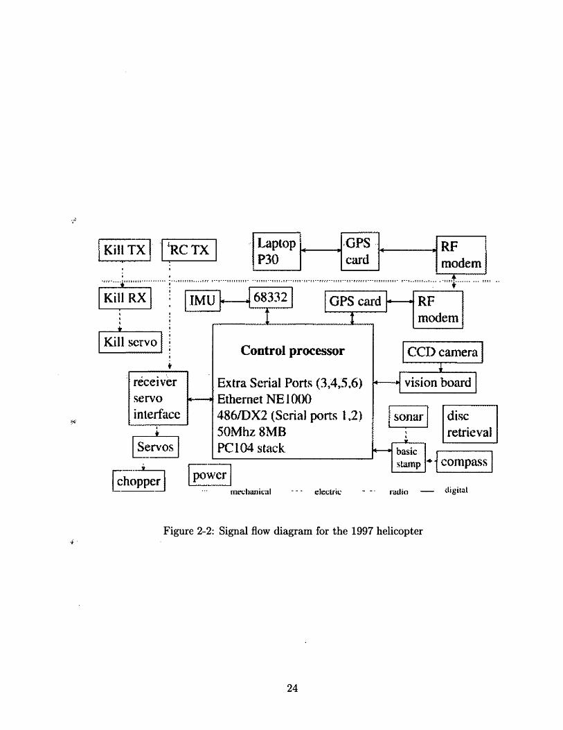
Signal Flow Diagram
The signal flow diagram is given in Fig 2-2. The important feature of the architecture
is use of only serial interfaces by the CPU. Each sensor requiring a more complicated
interface, is sampled by a lower level processor. The IMU is sampled by a fixed point
Motorola 68332 processor. The sensor interface was non-serial digital, and required
an external clock rate signal at 1 MHz, which would be impossible to provide with
the CPU. Basic Stamp was used to sample sonar altimeter and magnetic compass.
Basic stamp is a chip which can be programmed with a simple set of commands in
the Basic programming language. This architecture can be called distributed. It has
an advantage with respect to a centralized architecture, that uses the CPU to sample
sensors directly, because the CPU computing power is not required to perform input
sampling.
Kill TXI RC TX
L iLL Z~J I ~'Y
receiverservo Linterface
Servos
chopper
68332..LL._
power. rn chanival --- electric
GPS card - RFe
CCD camera
-- vision board
Isonar disc."retrieval
asicsstamp * compass
S rado -- igital
Figure 2-2: Signal flow diagram for the 1997 helicopter
Control processor
Extra Serial Ports (3,4,5,6)Ethernet NE 10()486/DX2 (Serial ports 1,2)50Mhz 8MBPC 104 stack
.. ...•i . ........... . .!. . . . . .. . . . . .. . . . .
Kill RX • IMU
Kill Srv IIKill .v

Both ground based and onboard GPS receivers have two serial ports, and uplink
and downlink commands are passed through from one port to another to insure the
line
laptop <- >GPS <->modem <- >modem <- >GPS < - >CPU
2.2.3 Selection Criteria for Navigation Sensors
The designer of an avionics system must go through a set of trade offs in the selection
process. The main considerations, common for all sensors are:
* performance requirements
* power requirements
* weight
* size, shape and volume
* cost
* ability to operate in the environment onboard an aerial vehicle
* ease of interfacing
The performance requirements for the sensors are derived from the attitude deter-
mination and navigation accuracy requirements. The designer must determine that
all of the important variables, including sensor drifts or biases, are observable from
the chosen set of measurements. The sensor set should have bandwidth at least a
decade above the vehicle dynamics. The correctly tuned estimation algorithm adjusts
its bandwidth to take information from each sensor at the frequency range where the
sensor performance is the best. The preliminary requirements on accuracy of sensors
are derived from measurement equations. For example a 5 mg accelerometer bias,
when used to correct low frequency gyro drifts, will result in a low frequency error in
estimation of local vertical of .005(180/7r) a 0.3 degrees. In more complicated cases,

the design of the estimation algorithm has to be performed and covariance simulation
run to determine the impact of errors. In the case considered in this chapter, the
set of navigation sensors consisted of the inertial measurement unit, GPS receiver
with base station for differential corrections, a sonar altimeter, and a magnetic flux
compass.
Inertial Measurement Unit (IMU)
The strapdown IMU provides high-bandwidth measurements of the vehicle inertial
angular rate and acceleration resolved into body axes. These measurements are used
for the inner loops of the control system, and for the time propagation of the naviga-
tion equations. The IMU is the heart of navigation system, and care must be taken
in making its selection. A detailed study of IMU use in unmanned helicopters is
given in [35]. Designs without an IMU were used in the past by Stanford University
teams, which relied on multiple antenna high update rate GPS receivers for attitude
information. The advantages of using an inertial measurement unit are a much higher
bandwidth, higher reliability and integrity. Other sensors, such as GPS receiver can
be used to compensate for IMU drifts, and to provide terrain information, in case
of sonar altimeter. For application to small aircraft, with short mission times, the
main performance characteristics of the IMU are bandwidth, short term bias stability,
scale factor errors, and noise. The performance tables for several inertial measurement
units are given in Table 3.2.
The noise level can be attenuated by choosing an A/D board with a larger number
of quantization bits, shielding analog lines from EM interference, and mechanically
isolating the sensor from high-frequency vibrations. A very important consideration
is the full scales for both gyros and accelerometers. The full scales should not only be
higher than the maximum accelerations and angular rates induced by vehicle dynam-
ics, but also exceed the residual vibration level, not damped by the mechanical filters.
The vibration level in a small aircraft can be as high as 10-100 g's, at frequencies as
low as 20 Hz. The main sources are engine vibrations and rotor misalignment. The
IMU should be put on flexures to reduce vibrations. An ingenious design of flexures

was suggested by Draper '96 team - the flexures were folded mousepads, which in
effect creates a second order low-pass filter. The vibration sources, like an engine,
should be isolated with anti-vibration mounts. In the example of vibration induced
by engine piston, the mount can be rigid in directions perpendicular to piston motion,
and very flexible in the direction parallel to it. If the residual vibration level does not
saturate the sensors, analog filters with roll off frequencies above vehicle dynamics can
be used. A higher sampling rate is beneficial to avoid aliasing of high frequency noise
from vibrations into the relatively low frequency region of the rigid body dynamics.
GPS receiver
A GPS receiver provides excellent low frequency position and velocity information,
especially in the horizontal plane. The receiver measures distances to the GPS satel-
lites, and then finds its position in earth-fixed coordinates by triangulation, using
accurate knowledge of satellite positions. Two sets of range measurements are used:
the time interval the signal travelled from satellite to the receiver (called pseudor-
ange), and the fractional number of the signal wavelengths (called carrier phase, or
integrated Doppler). The second measurement is obtained by integrating the Doppler
shift due to satellite motion, and contains the initial value of the integral (ambigu-
ity), which has to be determined. This value is an integer, and algorithms exist for
its resolution. The common error sources for GPS are the selective availability (SA),
which is a pseudo random noise signal introduced by US government, multipath (a
receiver mistakenly uses a reflected signal instead of the true signal), ionosphere and
troposphere delays. Using correction signals from a second GPS receiver, placed at a
known location, allows the elimination of SA and reduces the ionosphere and tropo-
sphere delays, provided the receivers are located close to each other. This technique
is called differential GPS, or DGPS. Also, receivers that use two standard frequencies
can correct for ionospheric delay, because it is frequency dependent. Choke rings
should be used for ground station antennas to avoid multipath errors and geodesic
tripods help as well.
The performance-based selection criteria for GPS receivers are the accuracy and
integrity (i.e. the continuity of the signal tracking without dropouts or failures).
Accuracy is provided by using DGPS, carrier phase measurements with integer am-
biguity resolution, and dual frequency receivers. Integrity depends on the receiver
technology used to keep track of satellites, and the number of satellites tracked by
the receiver. GPS/GLONASS receivers, for example, can provide better integrity
than GPS-only receivers because of the increased number of satellites available at
any point in the world. The satellite lock can be poor due to both antenna vibra-
tion and receiver vibration. The latter affects the performance of the oscillator, that
provides frequency reference for the receiver components. Loss of GPS track leads to
significant performance degradation of navigation solutions, and the IMU should be
good enough to keep the system operational until reacquisition. In the case of this
unmanned helicopter, the safety pilot should have several seconds to notice that GPS
track is lost and take over the control of the vehicle [19]. Longer reacquisition times
directly result in tighter requirements on IMU performance. The sampling rate of a
GPS receiver can be important if it is used without an IMU.
GPS technology leads to a significant reduction in the cost of avionics systems,
because the IMU drift requirements become much less stringent in GPS/INS systems
compared to a stand-alone INS. At the current state of technology, improvement in
IMU performance is very costly compared to improvement in GPS performance.
Surveys of available GPS receivers are published annually in [33].
Sonar Altimeter
The sonar gives high bandwidth altitude information by sending acoustic signal pulses
and measuring the signal return time. This information is used during landing. Se-
lection criteria are accuracy and bandwidth.
Magnetic Compass
A compass provides low frequency heading information by measuring the direction to
the local magnetic north. The criteria are accuracy and availability of tilt compen-
sation.
Non-performance based criteria
Great care should be taken in selecting avionics sensors for small UAVs based on
power requirements, size, and weight. The issue of power requirements for the IMU
and CPU was not given proper attention in 1997, and this led to increased battery
weight, a complicated power board design and extensive weight reduction of the
vehicle structure. The power requirements should be kept to as few voltage levels
as possible to avoid unnecessary power regulation. This is becoming increasingly
feasible, since most electronics tend to use a few standard voltages (e.g. ±5, ±12 V).
A detailed electronic system design for a small helicopter is given in [35].
Convenient sensor interfaces are vitally important. The time spent on develop-
ment of device drivers and analog prefilter circuitry directly results in program costs.
The simplest interface is a serial port. It is, at the same time, often inflexible because
it restricts sampling rate and does not allow analog prefiltering. The sampling rate
problem is likely to be mitigated with faster electronics. The sensor bandwidth and
internal prefiltering can usually be specified by the customer. In addition to saving
development time, another great advantage of a serial interfaces is its adaptability
for hardware-in-the-loop simulation. Reproducing analog outputs from a digital sim-
ulation can often be costly, in comparison to purchasing additional serial cards for
the simulation computer. An integrated simulation framework is suggested in Ap-
pendix A.
2.3 Guidance, Navigation and Control Algorithms
2.3.1 Algorithm Reuse
The 1997 and 1998 MIT teams used the same sensor configuration as MIT/Draper
Laboratory DSAAV (Draper Small Autonomous Aerial Vehicle) used in 1996. In
1997, the performance of the sensors was close to that of 1996 sensors, and the MIT
team completely reused the MIT/Draper '96 team algorithms for guidance, naviga-
tion and control (GN&C). The control logic employed in the 1996 design used a set of

proportional, integral and derivative (PID) inner control loops, and waypoints were
used for outer loop guidance. These algorithms were a result of 2 years of experiments
with autonomous helicopters, and proved to be robust, flexible and tunable in flight.
In 1997, the navigation algorithm, based on an extended Kalman filter (EKF), was
tuned by changing the measurement and driving noise covariance matrices. Naviga-
tion and control were run on board, and the guidance algorithm was run in a ground
station computer. The description of GN&C algorithms used in MIT/Draper 1996
helicopter system is given in [19].
In 1998 the sensor performance has changed considerably: the IMU, GPS and
compass were significantly different. The '98 Crossbow IMU had much larger biases
than the '96 Motion Pak and '97 GEC Marconi units. On the other hand, a Novatel
RT-2 receiver showed considerable improvement in performance with respect to RT-
20 due to higher reliablility of in-flight ambiguity resolution. Also, a TCMVR-20
magnetic flux compass from Precision Navigation gave better heading angle estimate
and provided direct measurements of roll and pitch angles. Thus, the need to update
'96 EKF has emerged and the detailed design of a new EKF for use in 1998 MIT
helicopter is given in the next section.
2.3.2 Extended Kalman Filter Design for Navigation of The
1998 Helicopter
Selection of States
The navigation computations are performed using two reference frames: a local north-
east-down (NED) frame, with the center of coordinate system chosen at the location of
the GPS base station, and an aircraft body frame with its origin at the aircraft center
of mass, X axis forward and Z axis down. The DSAAV navigation algorithm [19] used
11 states. Three more states, corresponding to gyro biases were added to account for
poorer IMU performance. The resulting state vector is
X= XL YL ZL UB VB WB q0 q1 q2 q3 g9 71 2 3] (2.1)

where XL, YL, ZL are vehicle positions relative to the ground station in NED frame,
UB, VB, WB are body axis velocity vector components; qo, q1, q2, q3 are a quaternion
representation of attitude, g is a gravity acceleration estimate, y1, 72, 73 are gyro bias
states. Gravity acceleration state implicitly accounts for accelerometer biases and thus
improves the attitude estimate [29]. The quaternion is a minimal representation of
attitude which is free of singularities. However, there is a recurring need to normalize
the quaternions after each time propagation or measurement update step:
q (2.2)
where= [qoq1 q2 q 3], and 1 12 =j q-.
Time Propagation Equations
Between measurement updates the state estimate is propagated using the nonlinear
differential equation:
S= f ( d, , a) (2.3)
where Z are the rate gyro measurements and a are the accelerometer measurements.
The inertial sensors are precalibrated before flight to account for biases. The inertial
unit should be given a 20 to 40 minute warm up time to avoid transient temperature
dependent bias and scale factor changes, at which point the calibration procedure
could be started. Estimates of body rates and accelerations are formed from sensor
outputs in flight:
WB = WIMU X SF w - Wbias
aB - aIMU X SFa - abias
where SF, and SFa are gyro and accelerometer biases. Accelerometer measurements
must be transferred to c.g. location to correct for the IMU moment arm (Appendix B).
Define the following vector arrays PL = [XL YL ZL, VB = [UB VB WB], q = [q0 q1 q2
qa], g = [0 0 g], 7 = [71 72 73]. Define a coordinate transformation matrix:
q0 + q - q- q3 2 (qlq 2 - qoq3 ) 2 (qlq3 + qoq2)
C 2 (q1 q2 + qoq 3) q2 - q2 + q2 - q3 2 (q2q3 + qoq1)
2 (qiq 3 - qoq 2 ) 2 (q2 q3 - q0oq) q - q - q + q 2
Define 3D and 4D skew-symmetric matrices for 3D vectors:
Q4 =
Then nonlin
0
-WY
Wz
We
0
Wz
-Wy
Wy
-Wz
0
Wx
Wz
WY
-Wx
0
1 4 =
0
-YX
-YZ
7YX
0
7z
-%y
0 -W z W 0 -- Y
-3 = WZ 0 -wx F3 = YZ 0
-wy Wx 0 -/y 7x
ear propagation equations can be written as:
PL
VB
_C B
= + C1g - (Q3 - F3 ) UB
2 (Q4 - r4)2(2.7)
g= 0
7= 0
These equations can be numerically integrated at the IMU sampling rate using a first
or second order integration routine. The IMU sampling rate of 25 Hz proved to be
sufficient using a first order integration routine.
The nonlinear propagation equations can be linearized, with the Jacobian matrix
A (, x, , =)19X
(2.8)
This matrix is used to propagate the error covariance matrix between measurement
(2.4)
7Yz
0
Yy
-z
0
7x
0
(2.5)
(2.6)
updates:
P = A(, )P + PAT(2, 0) + Q (2.9)
where Q is the process noise intensity matrix, which is used to model errors of inertial
sensors. Typically the Q matrix is chosen to be diagonal. The suggested initial guess
for main diagonal values is derived from sensor covariances:
Qd l[ 2 2 I x4 2 1 ] (2.10)
where Oa, a9 are the estimated accelerometer and gyro noise rms values, and cab,
agb are bias stability rms values, and 7 is the sampling rate of inertial sensors. The
scaling by 1/T is needed to account for the fact that the equations are integrated
numerically with time step 7 [14]. The a parameters can be used to tune the system
for maximum performance.
A first order integration of equations 2.9 proved to be satisfactory. The continu-
ous propagation equations can be discretized, and a discrete version of propagation
equations can be used [14]. The Jacobian matrix A is a sparse matrix, given in
Appendix B.
Measurement equations
At the instances of time when the updates of DGPS, sonar altimeter or compass occur,
the measurement update equations are used. Let h(x) be the nonlinear measurement
function of state, and let
H Oh(x) (2.11)
Then the EKF measurement update equations are given by [14]
K = PHT [HPHT + R]
2+ = - + K [z - h(i)] (2.12)
P+ = P- KHP

where K is the filter gain, R is the measurement noise covariance matrix, and z
is the measurement. In some instances the inversion of the symmetric matrix in
equation 2.12 may become close to singular, so the computer may not have a sufficient
number of bits (16 would be marginal) to assure positive eigenvalue. In this case the
computations are unstable, so the square root implementation of the KF should be
used [14].
DGPS is used to correct low-frequency drifts in position, velocity and attitude
estimates. The sampling rate of the RT-2 receiver is 4 Hz. DGPS provides anntenna
position and velocity information in the local NED frame. This data must be trans-
ferred to the vehicle c.g. location (Appendix B). The linearized equations for GPS
measurements are:
Hp= [ 3x3 03x3 03x4 03x1 03x3 (2.13)
H= [ O3x3 C Hvq 03x1 03x3 ] (2.14)
The block Hvq is given in Appendix B. Standard deviations of position and
velocity measurement are provided as outputs from the GPS receiver. These estimates
take into account the current state of the internal receiver KF, whether ambiguities
are resolved, the number of satellites etc. These values are used to determine the
measurement noise covariance. Under normal operating conditions, when the estimate
has converged, the standard deviation of horizontal position measurement error is
up = 0.02 m, and horizontal velocity measurement error standard deviation is av =
0.003 m/s for RT-2 receiver. Vertical position and velocity error standard deviations
maybe 3-4 times larger than horizontal. In the data sheets for RT-2 receiver the
specified time to convergence after GPS acquisition is around 12 min if at least 6
satellites are available, thus the receiver should be started during the IMU warm-up.
DGPS provides altitude information relative to the location of the base receiver.
To take into account terrain information during landing, the sonar altimeter is used.
Sampling rate for the sonar is chosen to be 5 Hz. The altimeter measurement updates

are used only if the measured altitude is between 0.5 m and 6 m. The altimeter
sends a pulse and shuts down so that it does not mistakenly take the emitted signal
for the reflected one. This explains the lower limit on sonar measurements. Sonar
measurements are also transferred to c.g. location (Appendix B). The standard
deviaton of sonar measurement error increases with altitude, at low altitude it is orh
10 cm due to grass and other surface non-uniformity. The linearized measurement
equation is:
Hh [ 0 0 1 01x3 01x4 Ox 01x3 ] (2.15)
For the case of a non-maneuvering vehicle, the heading angle is unobservable in
the GPS velocity measurements (see Section 3.7.2). Magnetic compass updates are
used to correct low-frequency drifts of the heading angle estimate. A sampling rate
of 1 sec is sufficient. The TCMVR-20 compass also provides roll and pitch angle
estimates. These are used inside the compass to correct heading information for tilt.
However, if CPU time allows, these measurements can be used in the EKF as well.
The compass measurement is corrected for magnetic variation, i.e. local direction to
magnetic North with respect to true North. The accuracy for compass measurement
is cr p 2 degrees. The linearized measurement equation for heading measurement is
He = [ 01x 01x3 Hq 01 01X3 ] (2.16)
where Hoq is given in Appendix B.
2.4 Software Architecture and Reuse
A major part of the onboard and ground station software from the 1996 system
was reused. Both ground station and onboard software were implemented in the
C programming language under the QNX operating system (OS). The QNX OS is
a multitasking operating system, allowing several independent processes to be run
simultaneously.
In retrospect, the decision to reuse the software was not justified. A summary of
the major functions of the '97 software is presented and the reasons why it was hard to
reuse the '96 software are given in the following paragraph. Ways to improve software
design for an unmanned helicopter are suggested as well. Detailed descriptions of the
'96 onboard and ground station software is given in [19].
The three major functions of the onboard software were navigation, control and
communication. The ground station functions include mission planning, waypoint
guidance, processing of vision information, communication, and the operator inter-
face. The vision processing code takes information from the Cognachrome vision
board, indicating the location of orange pixels in the camera field of view. It decides
whether there is a disc, and estimates the disc coordinates based on the current state
of the helicopter. The mission planner adds this location as a new entry into waypoint
list. The guidance logic converts the waypoint list into low-level position, velocity and
heading commands for the onboard control loops. Implementing the guidance logic in
the ground station introduces a delay, and it is recommended that it be incorporated
onboard the vehicle.
Figure 2-3 illustrates a high level flow chart for the onboard software. The onboard
processor communicates with the external devices via serial ports, using non-blocking
I/O. This means that the main program will not hang up in case the device being
sampled fails. This is an important safety feature. However, it would be logical to
use the multitasking capability of QNX OS to have separate processes for interfacing
with devices, for control and navigation logic, and for communication. This would
allow better timing for the processes, and easier debugging due to higher modularity.
A good rule for software engineering is to keep different functions in separate files,
otherwise the code becomes very hard to debug. With the exception of interfaces,
all code that implemented the flow chart above was contained in a single file, which
made this software difficult to reuse.
A simple example of the multitasking design approach to the onboard software
for unmanned aircraft is given in Section 3.4.
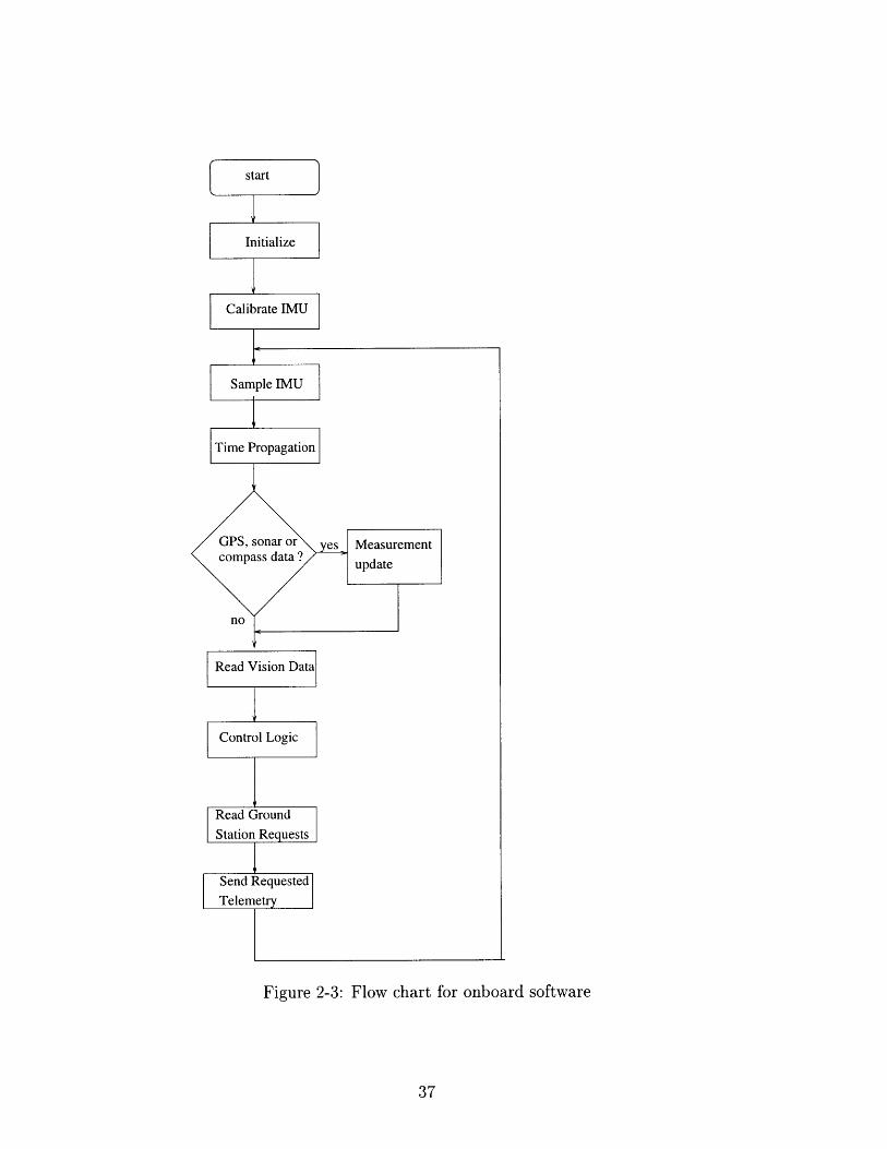
Figure 2-3: Flow chart for onboard software
37

38
Chapter 3
Gun-Launched Surveillance
Aircraft
3.1 Wide Area Surveillance Projectile
3.1.1 Project Background and Goals
The avionics system development for an autonomous surveillance aircraft is pre-
sented in this chapter. The effort described here was done under the sponsorship
of Draper Laboratory as a part of the MIT/Draper Technology Development Part-
nership Project. The major goal of the project was to develop entrepreneurship and
innovation in engineering students. The primary requirement was to create an inno-
vative product that would meet a major US national need.
During the fall term of 1996 a team of students, MIT faculty, and engineers from
Draper Laboratory proposed several ideas, all related to aerospace. The group per-
formed market assessments and preliminary technical evaluations of the concepts,
and finally selected the Wide Area Surveillance Projectile (WASP) concept. WASP
is a small gun launched aircraft, designed to meet a need for fast-response surveil-
lance capability. A set of requirements for the vehicle was determined with potential
customers (Navy, Army, Defence Airborne Reconnaissance Office) and the sponsor
(Draper Laboratory). The requirements were further adjusted as the design pro-

gressed, and final estimates of the required performance are:
* 15,000 g launch environment
* 15 min. loiter time
* 15 km range
* 250 m radius of camera field-of-view, still frame or video image
* fit inside a 5" shell diameter
* 2-way datalink capability
* GPS-based waypoint guidance
In a typical scenario, WASP is launched from a 5" Navy gun, reaches its destination
point (15 km range, and altitude of 500 m), is deployed from its shell, and starts
sending still images or a videostream, and positioning information of designated points
to a ground station. A ground operator designates new waypoints for the vehicle and
commands its search pattern. Recognition of points of interest is performed by the
operator, and positions of points of interest are determined using a combination of
onboard navigation and camera pointing information.
3.1.2 Overall Design
This section provides a brief description of the overall vehicle design. A detailed
discussion of the structural design, deployment mechanisms and aerodynamic design
are given in [20] and [6].
The flyer is stowed inside a 5" fin-stabilized artillery shell, derived from a re-
designed illuminating round. At a predetermined time after gun launch an onboard
timer triggers separation of the shell base, and a parachute is deployed. The parachute
decelerates the vehicle to a sufficiently low dynamic pressure to allow deployment of
the wings, tail surfaces and a propeller. The vehicle is powered by a 2-stroke internal
combustion engine, which is started by a preloaded spring device. A drawing of the
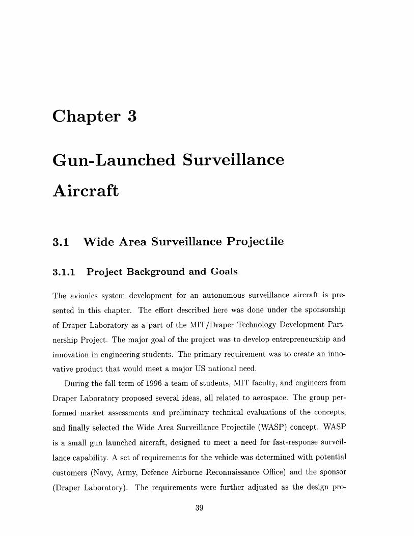
Figure 3-1: Deployed WASP flyer
flyer is given in Figure 3-1. There are two static vertical fins, one on the bottom and
one on top of the vehicle; and two downward pointing control surfaces, in a vee-tail
configuration, which provide lateral-directional and longitudinal control. The fins
were added to improve lateral-directional weathercock stability. The wings have a
nominal dihedral angle of 3 degrees.
The onboard avionics system includes a tightly coupled GPS/INS system, a 2 way
datalink and a charge-couple display (CCD) camera. A detailed description of the
avionics is given in Section 3.2.
3.1.3 Testing Approach
To demonstrate the key capabilities of the proposed system, two prototypes were
developed: a high-g vehicle and a flight test vehicle (FTV). The requirements for
the high-g vehicle were to demonstrate the survival of the airframe and shell in the
gun environment, and to show operation of the deployment mechanisms. The high-g
vehicle does not have any avionics onboard. Micromechanical high-g-qualified avionics
systems for use in smart munitions programs are currently under development in
Draper Laboratory, but are not available for the WASP flight tests because of the
high cost. The WASP design relies on the future availability of these systems.
The other prototype, the FTV, was designed to demonstrate flying qualities and
aerodynamic performance of the deployed flyer. The preliminary stability analysis of
the WASP flyer showed that the flying qualities will present a challenge for the design
of a stability augmentation system. This is due to minimal lateral control authority
because there are no ailerons and small control surface area, and a near-stall incidence
angle of the wings.
The FTV is a scaled up test version of the operational flyer, equipped with off-the-
shelf avionics. It is not launched from a gun but rather deployed from a conventional
ultralight aircraft. It has a remote control receiver with an interface to the onboard
computer, and can be flown by a remote pilot with a control augmentation system.
The parameters of the prototype vehicle were chosen to match important stability
characteristics of the WASP (Section 3.5.10). The "scaling-up" approach, used in
the project to achieve dynamics similarity of the vehicles, can be a useful tool for
development of a small unmanned aircraft, it provides a relatively low-cost and high-
fidelity solution to testing and data gathering.
3.2 Hardware Architecture for the Operational
Vehicle
A set of specifications for the WASP avionics systems was derived from the perceived
customer requirements, stated in Section 3.1.1.
* digital flight control system
* GPS/INS navigation and control
* onboard imaging system
* 2-way encrypted datalink

All avionics must survive 15,000 g. The Draper Laboratory developed high g-
qualified integrated INS/GPS navigation system for Extended Range Guided Mu-
nitions (ERGM) program and another follow on advanced technology demonstrator
(ATD) program, which will provide the technology for the core avionics for the WASP.
Both the ERGM and ATD systems use a micromechanical inertial sensor assembly
(MMISA), and a DSP-based GPS receiver. The flight control computer is also a
g-hardened DSP chip. The fact that these systems are being developed at Draper
Laboratory was a major advantage in pursuing the gun-launched surveillance aircraft
concept, because of the ready access the team has had to information and advice from
Draper engineers.
A CCD camera will be used as an imaging sensor. A high-g CCD camera is
being developed by Xybion Corporation. Two COTS CCD cameras (Black & White
Pro-Video CVC-50PH, Black & White Watec WAT-660) survived air-gun testing at
15,000 g's. Thus there will potentially be a choice for a high-g qualified imaging
sensor.
Separate C-band receiver and transmitter are suggested for the two-way datalink.
A message forming encryption chip, that takes telemetry information from the flight
control computer and video information from the CCD camera will relay data to the
ground via the downlink transmitter.
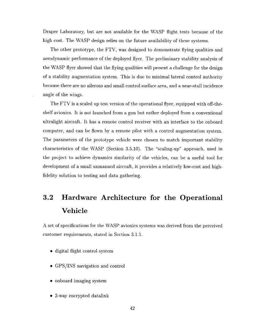
The signal flow diagram for the operational WASP is presented in Figure 3-2.
3.3 Hardware Architecture for the Flight Test
Vehicle (FTV)
3.3.1 Requirements and Constraints
The initial set of requirements for a prototype vehicle included a demonstration of au-
tonomous flight, with a minimal requirement to demonstrate that the vehicle can be
flown by a remote control pilot, with the help of an onboard stability and control aug-
mentation system. Although the FTV uses off-the-shelf electronics its aerodynamic
Signals- electrcal- - - radio
..... ...... mechancal
Rght upik uplik plnkINS Control recver trmn er
Computer
Downlink downlink dowlinkConpumtr mtnsinmlner C.nt u er
Figure 3-2: Signal flow for operational WASP
shape is kept as close as possible to the deployed configuration of the operational ve-
hicle. FTV is not required to demonstrate deployment mechanisms. The same servo
gears and a similar 2 cycle internal combustion engine are used in the FTV. Also, both
the FTV and the operational WASP do not have landing gear. The FTV deployment
is done from a remotely piloted, powered, ultra-light aircraft; under command from a
ground based operator. The retrieval is done by deploying a parachute from the base
of the FTV. A digital control system allows tuning of control algorithms in flight and
gathering flight test data.
The vehicle was a x1.28 scaled up copy of the operational WASP. The volume
constraint was very important for FTV. The allocation of weights inside the FTV was
done to keep the dynamics of the flyer similar to that of the operational WASP. The
vibrations induced by the engine piston motion and propeller unbalance are important
factors in development of the FTV.
3.3.2 Subsystems
Sensors
The inertial measurement unit was chosen to provide high-bandwidth information
for the stability augmentation system and attitude information for the autopilot. To
meet the requirement for autonomous flight, the Systron-Donner Motion Pak was
chosen. The main performance characteristics of the unit are given in Table 3.2. Mo-
tion Pak has analog outputs and requires an A/D card onboard the aircraft to provide
an interface to the onboard computer. A mistake was made during the selection of
accelerometer full scale ranges: they were chosen to match vehicle dynamics only. As
was mentioned in the Section 2.2, it is necessary to choose the full scale of accelerom-
eters higher than the vibration level that can be experienced in the vehicle. Because
the sensitivity was chosen to be quite high, relative to the vibration created by the
engine, the team had to design special anti-vibration mounts to reduce vibration level
below .1 g peak-to-peak. These mounts were used to isolate the engine from the nose
cone, and the nose cone from the fuselage. However, in spite of the anti-vibration
mounts a 100 Hz vibration component, from propeller unbalance, still remained a
problem. To fix it, the IMU was mounted on a series of folded rubber sheets. This
effectively creates a flexure that acts a fourth order lowpass filter, and guarantees a
-80 dB/decade slope at high frequencies. Finally, when saturation of IMU was no
longer a problem an active analog low pass filter, with 8 hz bandwidth, was used to
filter out residual high frequency vibration. The sampling rate was increased from 50
hz to 100 hz to avoid aliasing.
To achieve autonomous operation, differential GPS was chosen to correct for IMU
drifts and provide heading information indirectly. Section 3.7.2 describes an attitude
and heading estimation algorithm that uses IMU data and GPS velocity information.
The G12 GPS receiver provides 1 m SEP position accuracy and .01 m/sec velocity
accuracy in the differential mode. It has a 2 second reacquisition time. The inertial
system has sufficient performance to provide adequate navigation during short GPS
dropouts.
Communication
Radio modems were chosen to provide two way communication links over a 1 mile
range. The modems have serial interfaces, and they are either directly attached to
the CPU, or their outputs go through the GPS receiver serial ports.
Computer Stack
A PC-104 stack, described in Section 2.2, was used as the communication bus for
the onboard electronics. The stack included a 486DXi 100 MHz CPU from Ampro
Computers, a 12 bit A/D card from WinSystems, a power supply from Tri-M engi-
neering and ethernet card with boot ROM from Florida DataMation. The 100 MHz
processor speed gives a significant advantage in onboard computing power and allows
IMU output sampling at more than 100 Hz. By comparison, the 50 MHz processor
used in the unmanned helicopter project, described in Chapter 2, could not handle
more than a 25 Hz sampling rate, resulting in marginal performance.
The VGA PC104 video card was used in table top testing for troubleshooting of
the stack electronics. As mentioned in Section 2.2, it allows one to connect the CPU
to a monitor and look at the program outputs directly, not via Ethernet link with
ground station computer.
Remote Control Unit
Standard model aircraft remote control servos were chosen to drive the differential
stabilizers. The torque requirements, weight and size were the main drivers in the
choice of the servos. The Futaba PPM receiver and interface, as described in Sec-
tion 2.2, were used to deliver pilot commands to the computer, and for computer
commands to the servos.
Retrieval Mechanism
A parachute deployment, to allow safe retrieval of the FTV, is commanded by an RC
servo via computer or pilot command.
Power System
During the process of choosing components special attention was given to minimizing
the number of voltage levels used, and the total power requirements as well, so as to
minimize battery weight. The complete design of the power system is given in [17].

Table 3.1 lists power requirements for the subsystems.
Component Power (W) Voltage (V) Tolerance (%)
GPS receiver 1.40 5 5GPS antenna 0.75 5-15 N/A
IMU 3.50 15 203.50 -15 20
CPU 4.90 5 5Ethernet 2.00 5 5
Serial Ports 2.00 5 5A/D 0.05 5 5
0.12 12 50.12 -12 5
Modem 1.00 5 5Total 19.64
Battery Efficiency x 1.2Conversion Efficiency x 1.33Total Power Required 31.34
Table 3.1: Power Requirements For Prototype Vehicle
The RC receiver and FPGA draw power from a separate battery. The cards in
the PC-104 stack are powered by a PC-104 power supply, which draws voltage in a
10-20 V range from the main battery. The GPS antenna is powered by the receiver.
Figure 3-3 shows the signal flow for the FTV.
3.4 Software Design for the Prototype Vehicle
3.4.1 Functionality
A good software design is essential for system integrity and safety. For example,
the prototype vehicle retrieval mechanism is a parachute, and the deployment of the
parachute is commanded via the CPU. If the parachute is not deployed the vehicle will
be destroyed, and could pose a hazard to people or the environment. An effective and
well documented software design increases productivity of the software development,
reduces the chances of unpredicted software behavior, and can save considerable de-
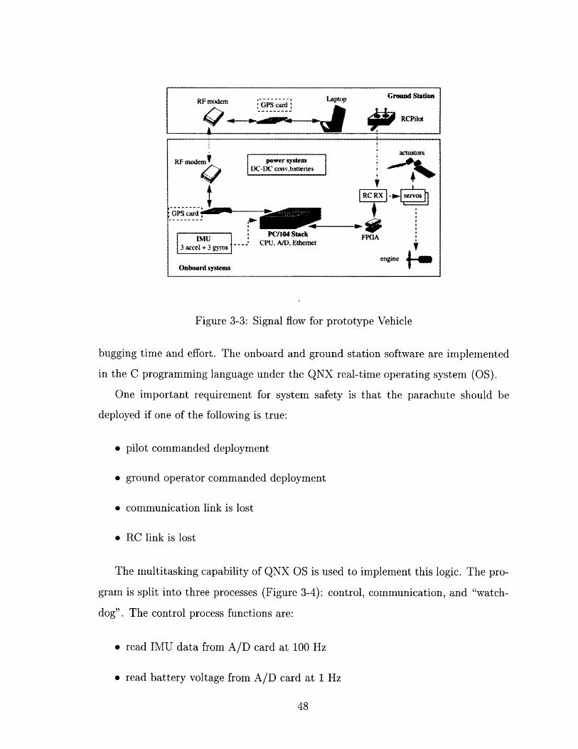
Figure 3-3: Signal flow for prototype Vehicle
bugging time and effort. The onboard and ground station software are implemented
in the C programming language under the QNX real-time operating system (OS).
One important requirement for system safety is that the parachute should be
deployed if one of the following is true:
* pilot commanded deployment
* ground operator commanded deployment
* communication link is lost
* RC link is lost
The multitasking capability of QNX OS is used to implement this logic. The pro-
gram is split into three processes (Figure 3-4): control, communication, and "watch-
dog". The control process functions are:
* read IMU data from A/D card at 100 Hz
* read battery voltage from A/D card at 1 Hz
RF modem power system ua
DC-DC convbatteries
RC RX ' AD
IMU M 4StackAI ... CPU, A/D, hefmet
engineOnboard systems
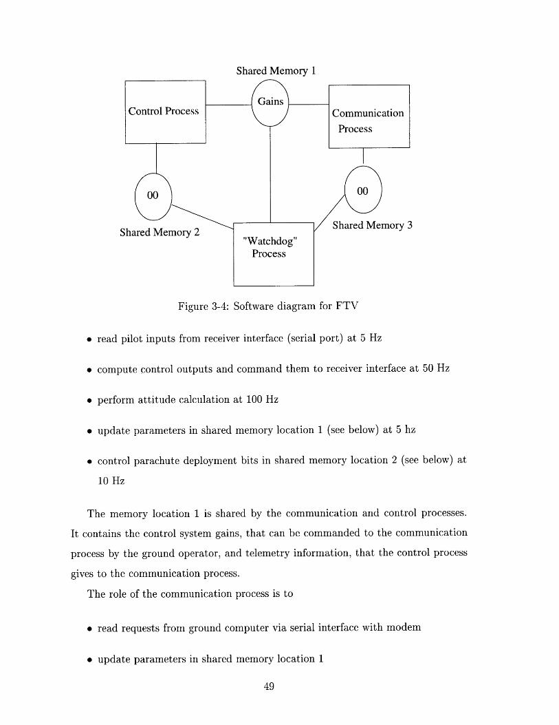
Shared Memory 1
Shared Memory 2Shared Memory 3
Figure 3-4: Software diagram for FTV
* read pilot inputs from receiver interface (serial port) at 5 Hz
* compute control outputs and command them to receiver interface at 50 Hz
* perform attitude calculation at 100 Hz
* update parameters in shared memory location 1 (see below) at 5 hz
* control parachute deployment bits in shared memory location 2 (see below) at
10 Hz
The memory location 1 is shared by the communication and control processes.
It contains the control system gains, that can be commanded to the communication
process by the ground operator, and telemetry information, that the control process
gives to the communication process.
The role of the communication process is to
* read requests from ground computer via serial interface with modem
* update parameters in shared memory location 1

* write requested and default telemetry to modem port
* update chute deployment bits in shared memory location 3
The watchdog process has access to shared memory locations 2 and 3. Both
contain only 2 bits. The first bit is the command from the other process sharing
location to deploy the parachute. The command can come from the pilot through
the control process, or from the ground operator through the communication process.
The second bit in each location is a health bit. The watchdog process resets both
health bits to 0 each time it runs. The other process sets it back to 1. In the event that
the health bit remains 0 more than a certain threshold time, the watchdog process
deploys the chute.
3.4.2 Implementation Issues
Shared Memory
The use of shared memory can pose a serious danger if not handled properly. Each
process, before reading from or writing to a shared memory location, must lock the
location, and unlock it after update is made. If this is not done, a race condition
may occur in which one process may read data while it is being changed by another
process. Thus, the value of the data can be completely erroneous. The FTV shared
memory is implemented using "shmemopen" and "mmap" functions of the Watcom
C compiler.
Timing
The timing can be done using "signals", which have the same meaning in QNX as in
UNIX, or by "proxies", which are QNX versions of interrupt. Each of these requires
a per-process timer. The timer is periodically reloaded, and when it expires, it sends
either a proxy or a signal, which triggers the run of the process.
In this design, all functions inside a process are run at multiples of the time period
the process itself is run. Thus simple counters can be used to trigger the lower rate
functions. The timer is created by the "create_timer()" routine.
Creation of Processes
Processes are created by the "fork" routine. For example, the "watchdog" is a parent
process, it creates a copy of itself using "fork". Then this copy is substituted with
the child process, which is either the communication process or the control process.
The watchdog timer is chosen to be a parent process for both of the other processes
because it should have access to shared memory locations with each of the processes.
3.5 Model and Simulation Development
3.5.1 Approach to modeling
This section describes the development of a common simulation framework for both
vehicles, provides a discussion of the linearized dynamics, and a description of the
stability and control augmentation system design.
It was decided to create a 6 degree of freedom (DOF) nonlinear simulation of both
flyers, find nominal trim conditions, and linearize numerically around the trim con-
ditions to obtain linear lateral-directional and longitudinal vehicle dynamic models.
The following features were incorporated into the simulation:
* 6 degree of freedom rigid body equations of motion
* aerodynamic forces and moments
* simplified engine thrust and torque model
* non-linear actuator models
* non-linear sensor models
* wind gust models
A description of these items is provided in the following subsections. The next sub-
section gives inertial and geometric properties for both vehicles.
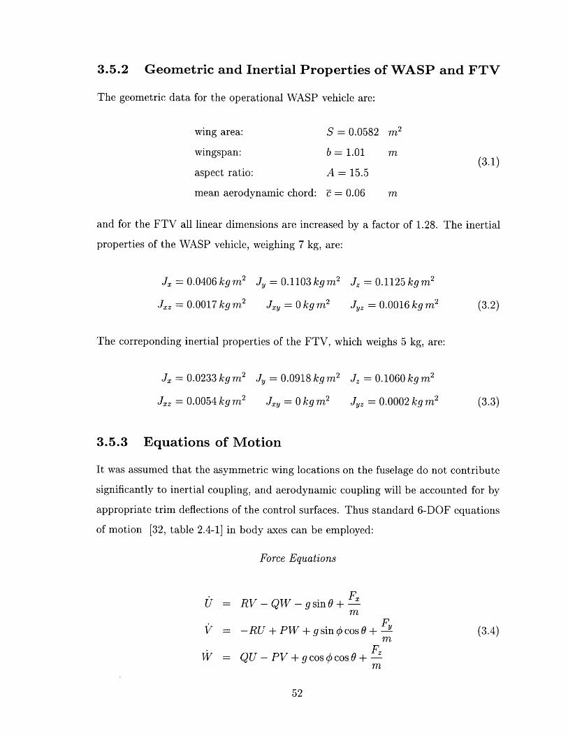
3.5.2 Geometric and Inertial Properties of WASP and FTV
The geometric data for the operational WASP vehicle are:
wing area:
wingspan:
aspect ratio:
mean aerodynamic chord:
S = 0.0582
b = 1.01
A =15.5
= 0.06
and for the FTV all linear dimensions are increased by a factor of 1.28. The inertial
properties of the WASP vehicle, weighing 7 kg, are:
J = 0.0406 kg m 2
JAX = 0.0017 kg m 2
J, = 0.1103 kg m 2
Jxy = 0 kg m 2
J, = 0.1125 kg m 2
yz = 0.0016 kg m 2
The correponding inertial properties of the FTV, which weighs 5 kg, are:
Jx = 0.0233 kg m 2
JXz = 0.0054 kg m 2
J, = 0.0918 kg m 2
Jy = 0 kg m 2
Jz = 0.1060 kg m 2
Jyz = 0.0002 kg m 2
3.5.3 Equations of Motion
It was assumed that the asymmetric wing locations on the fuselage do not contribute
significantly to inertial coupling, and aerodynamic coupling will be accounted for by
appropriate trim deflections of the control surfaces. Thus standard 6-DOF equations
of motion [32, table 2.4-1] in body axes can be employed:
Force Equations
FRV-QW-gsinOU = RV -QW-gsinO+ x
V = -RU+PW+gsinocosO+ "2m
S= QU- PV + gcoso cos +m
(3.4)
(3.1)
(3.2)
(3.3)
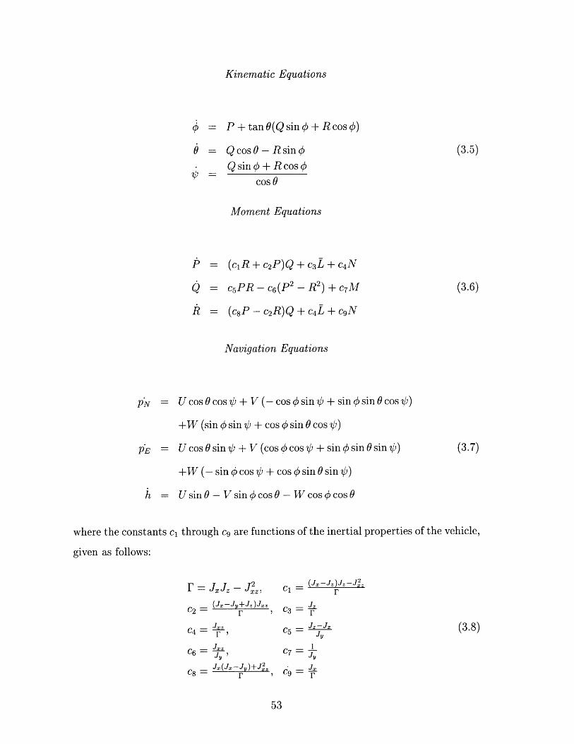
Kinematic Equations
= P+tanO(Qsin +Rcos )
0 = QcosO-Rsin
Q sin ¢ + R cos ¢cos 0
Moment Equations
P = (cR + c 2P)Q +c 3L+ c 4N
Q = c5PR-c 6 (P 2 -R 2 ) +c 7M
R= (c8 P - c2R)Q+ C4L + c9N
Navigation Equations
PN = U cos 0 cos + V (- cos 0 sin 4 + sin sin 0 cos )
+W (sin q sin 4 + cos q sin 0 cos 4)
p E = U cos 0 sin + V (cos cos V + q$s sin 0 sin ')
(3.5)
(3.6)
(3.7)
+W (- sin q cos 4p + cos ¢ sin 0 sin 4)
= UsinO - VsinqcosO - WcosbcosO
where the constants cl through c9 are functions of the inertial properties of the vehicle,
given as follows:
C4 = JJ - J
Fc2
c4 ,
J. 2C6 -jy
Jx(Jx-J )+J zcs - r
Cl (Jx-Jz)Jz-Jr
JzC3 -r
C5 =Jy
1C7 Jy
C --ix
(3.8)
3.5.4 Aerodynamic Forces and Moments
Non-dimensional aerodynamic coefficients were estimated using a variety of tools.
The complete set of coefficients was broken down into 4 subsets:
* constant force and moment coefficients calculated using potential flow theory
* control derivatives
* drag coefficients
* forces and moments that depend non-linearly on angle of attack
Both the operational WASP and FTV fly at a low subsonic Mach number (M < 0.15),
and the flight altitude does not change significantly during operation. Thus, as long as
the aircraft does not stall, the only parameter that affects the aerodynamic coefficients
is center of gravity (cg) location. The cg changes with time, as fuel is burned, and
its change of location primarily affects the pitching moment due to angle of attack
coefficient - C,,. The center of gravity changes from 20.3 cm forward of the back end,
with a full fuel tank, to 20.0 cm forward of the back end, with an empty fuel tank.
This change represents 5 percent of the mean aerodynamic chord and it is accounted
for in the simulation. Also, it is reasonable to assume that both FTV and WASP have
the same values of aerodynamic coefficients, because Mach number is not a relevant
parameter at M < 0.15, and drag derivatives do not affect stability.
Coefficients calculated using potential flow theory
These coefficients were estimated using the Athena Vortex Lattice program (AVL).
The value for C,, given here is at the most aft cg location, and it is calculated
at each timestep of the simulation, using the current estimate of the fuel weight.
The simulation equations are integrated with a variable time step, determined by
Simulink to better represent continuous dynamics. It is assumed that the fuel weight
is changing according to the following ODE:

-KfuetT ifx > 0
S0 otherwise
where T is a throttle setting in Watts and
Kfuel = Wfuel (3.9)Tmaxtexp
where Wfuel is initial fuel weight, Tmax is maximum throttle setting, and texp is time
(in seconds) it takes to burn a full tank of fuel at full throttle. The c.g. location of
the vehicle, due to fuel burn, is determined from the following equation:
Xvf =mvXvmfXf (3.10)m, + mf
where m, - weight of the vehicle without fuel, Xv - c.g. of empty vehicle, mf - fuel
weight, Xf - fuel tank c.g. The change in Cmn is given by:
mf(xf - X,)S= (m C- X) CL (3.11)
(m, + mf)?
The remaining coefficients are all assumed to be constant and their values are as
follows:
Longitudinal Coefficients
CL = 6.261 CLq = 9.866
Cm = -0.163 Cm, = -13.188
Lateral Coefficients
Cy, = -1.007 CI, = -0.085 Cn = 0.015
Cy= -0.119 C1, = -0.729 Cn, = -0.162
CY, = 0.488 Ci, = 0.420 Cn, = -0.083

The accuracies of these estimates are consistent with currently available methods for
predicting stability derivatives based on both purely analytical methods and numeri-
cal finite element calculations, where appropriate. For example, the value of lift curve
slope CL, = 6.261, obtained with a vortex lattice method, is probably an overesti-
mate, since this slope is not likely to be so close to 27r, for a three-dimensional vehicle.
However, the value for the static margin cL, obtained using an estimation formula,
was verified independently with wind tunnel tests and gave very close results. For
most aircraft configurations, the vortex-lattice method tends to give stability deriva-
tives within 15 percent of their true values. However, the AVL representation of
WASP contains a crude model of the fuselage, which is represented by two intersect-
ing plates rather than a body of revolution. A number of these kind of approximations
were made, which should be verified by wind tunnel and flight testing.
Control derivatives
The control derivatives were estimated using two independent methods. Analytical
values, based on traditional vehicle models, were compared with AVL values computed
for various surface defelctions. It was found that both methods produce consistent re-
sults for the longitudinal control derivatives. There was less consistency for the lateral
directional derivatives. The smaller values, obtained with the analytical techniques,
implied poorer flying qualities (smaller values of control derivatives correspond to
lower control power), and these values were used in the simulation.
Cm, = 1.27 CL, h = 0.5591
CY h = -0.1 C,'h = 0.009 Cn, = 0.01
Here longitudinal derivatives correspond to symmetric deflection of the differential
stabilizer, in which case the stabilizer acts like an elevator, and lateral derivatives
correspond to antisymmetric deflection, in which case the stabilizer acts like a rudder.

Drag derivatives
Drag was estimated both analytically and in the wind tunnel. The analytical predic-
tion tended to overestimate drag, and wind tunnel data are given here for drag at zero
angle of attack: CD = 0.0881. The induced drag formula is used for computation
at each timestep, because induced drag depends on lift coefficient, which varies with
angle of attack.
Coefficients with non-linear dependence on angle of attack
At each timestep during the simulation, angle of attack a, angle of sideslip /, as well
as projections of angular rates onto aircraft stability axes are computed. After the
lift coefficient is computed, its value is used to compute induced drag. The induced
drag component stems from empennage drag, induced drag on the wings, and induced
drag on fuselage. Induced drag on wings is given by
CDL L2rA (3.12)
where e = 0.8 - efficiency factor, A = 15.5 - aspect ratio, CL - lift coefficient, given
by equation 3.17. Induced drag on fuselage is calculated as
CDL = 2a2 S b s + CDc a3Spus (3.13)fus S S
where Sbfs = 0.0125 m 2 - fuselage base area, and Sp,, = 0.0672 m 2 - fuselage
planform area, r = 0.65 - ratio of the drag of a finite cylinder to the drag of an infinite
cylinder, CD - experimental steady state crossflow drag. To determine induced drag
on the tail it is necessary to obtain lift generated by the tail:
tr + ZiCLh = CLh ( + 2 ), (3.14)
where CLah = 4.71 - empennage lift slope, ir and il - right and left stabilizer deflections
(positive down), so (i, + it)/2 = 6e - effective elevator action. The induced drag on
the tail is:C St cos 6
CDL h - (3.15)Lemph = rAhehS
where St = 0.0119 m 2 - tail area, 6 t = 35 deg - tail anhedral, Ah = 3.89 - tail aspect
ratio, eh = 0.7 - tail planform efficiency factor.
Dimensional Forces and Moments
At each simulation timestep, aerodynamic forces and moments are computed using
standard dimensionalizing formulae. First, angular rates are transformed to stability
axes:
Ps = Pcosa+ Rsina
Q = Q (3.16)
Rs = -Psina+Rcos a
The lift coefficient is obtained as:
CL = CLo + CL - CL ,h (i $ Et) CL if CL < CL(3.17)CL 2Vr (3.17)CLmx otherwise
where CLo = 1.4726 - zero angle of attack lift coefficient, CL'h = 0.5591 - tail lift
curve slope, Vr - current velocity, ct - downwash angle, assumed to be constant at 0.1
deg. CLmax = 1.91 - maximum lift coefficient used for crude modeling of stall. The
lift force is obtained from Fz = -CLqS.
The total drag coefficient is:
CD = CDO + CDL + CDLfs + CDLe,,ph (3.18)
The aerodynamic force in the X-direction in stability axes is Fx = -CDqS.
The aerodynamic force coefficient in the Y direction is:
SPb Rb t (3.19)Cy = CY + CY2, + Cy T2 + C - (3.19)

and the Y-axis force is Fy = CyqS.
Then the forces are transformed from stability axes into body axes:
Fxb = Fx cos a - F, sin a
Fyb = Fy (3.20)
Fzb = Fzsin a + Fzcos a
Similar equations are developed for aerodynamic moments: The rolling moment
coefficient is:Psb Rb
C1 = CO + C , + C R,2 Vcr 2 Vc
+ C, ( 2 ) (3.21)
Rolling moment in stability axes is Ls - CqqSb.
The pitching moment coeffcient is given by:
C L+ QC s ccm = Cmo + --- CL + cmq2CL, 2 V2r
+ Cmh ( + it2 )
where Cm0 = -0.0688 - pitching moment coefficient at zero lift, zero stabilizer deflec-
tion. The aerodynamic pitching moment in stability axis: Ms = Cm-S-.
The yawing moment equation is:
PsbCn = Cn,3/ + Cn P2
' 2Vcr
Rsb+ Cfr 2V + Cn,h ( 2 )
The aerodynamic yawing moment in stability axis: Ns = Cn-qSb.
Then the moments are transformed from stability axes to body axes:
Lb = Lscosa-Nssin a
Mb = M
Nb = L sin a + Nscos a
(3.22)
(3.23)
(3.24)

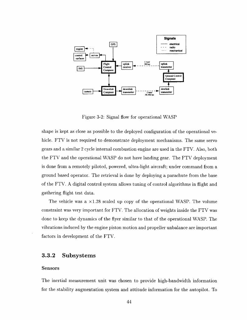
WASP engine FTV engine
15 , 20
z 10 Z 10
5 0
600 40 40040 2 400 30 200
velocity, m/s 20 0 power, watts velocity, m/s 20 0 power, watts
0.4 " 0.4
E 0.3-
-0.2E0.2 C
0.1 060 40
40 0 4004 30 200velocity, m/s 20 0 power, watts velocity, m/s 20 0 power, watts
Figure 3-5: Engine thrust and roling torque for WASP and FTV.
3.5.5 Engine Model
A simplified propeller model was built using a computer program called Xrotor, avail-
able on Athena (MIT computer network), which employs a potential flow calculation
method. Aircraft velocity and power setting are given as inputs to the program, and
thrust and rolling torque are produced as outputs. This is a fairly crude model for the
engine, but it will suffice for longitudinal stability analysis, because the only mode
affected by powerplant properties is a slow phugoid mode, which is not crucial for fly-
ing qualities. The WASP and FTV engine models are given here as two dimensional
tables which are illustrated in Figure 3-5.
3.5.6 Actuator Models
Simple actuator models, based on slew rate data for standard radio control model
servos were assumed for both vehicles. Each of the differential stabilizers was modeled
as follows:
* first order low pass filter with bandwidth of 15 rad/sec

. rate limit of 200 deg/sec
* deflection limits of ±10 degrees
The bandwidth of 15 rad/sec was chosen according to
full rangeactuator bandwidth 0 1.5 (3.25)
slew rate
3.5.7 Sensor Models
The position of the inertial measurement unit was determined for each vehicle, and
accelerometer measurement equations were defined. For stability augmentation pur-
poses, the important sensor properties are bandwidth, non-linearities, and noise. For
attitude determination and navigation, biases are also important. The following prop-
erties were modeled for both systems: first-order anti-aliasing filter, noise, saturation
at full scale and short term biases. The sources of noise are A/D board quantization,
EM noise in wires and inherent sensor noise, all of which is modeled as band-limited
white noise. Short term bias is usually modeled as a first order Markov process with
a large time constant. In cases when the time constant for bias stability is much
larger than mission time, a random constant model is assumed. Short term bias is a
residual bias after pre-calibration. If it is not specified in manufacturer specifications,
it must be measured. Three sets of sensors were modeled:
* micromechanical inertial sensor assembly (MMISA), projected for use in WASP
* Systron-Donner Motion Pak, used in FTV
* Crossbow DMU-6, used in FTV
Biase and noise 1 a rms value estimates for these units are given in table 3.2.
Other important considerations for sensor selection are highlighted in Section 2.2.

Error Units Crossbow I Motion Pak MMISAgyro bias deg/sec 0.01 0.004 0.003
gyro noise deg/sec 0.1 0.1 0.1accel bias mg 5 1 1
accel noise mg 5 1 1
Table 3.2: IMU Models
3.5.8 Gust Models
Stochastic gust models were taken from [5]. The gust models take into account
the dependence of the probability of gust occurrence on altitude. The estimate of
probability of encountering gusty air at sea level, given in [5], is 80%. The root mean
square gust velocity is assumed to be normally distributed with standard deviation
a = 2.3. Gust levels of 1 a were assumed for the model. Forward, vertical, and lateral
velocity gusts in aircraft body axis, as well as rolling gust were modeled as first and
second order Markov processes. The gust model shaping filters take into account
altitude, wing span and airspeed. These models were based on larger aircraft, and
their validity for a small aircraft as WASP or FTV is uncertain. The frequency
content of rolling gusts seems to be exaggerated according to this model. Thus, the
same shaping filter was used for rolling gusts and side velocity gusts. Shaping filters
for gusts are given in Fig 3-6.
3.5.9 Trim Analysis and Linearization
The non-linear 6-DOF simulation of the aircraft dynamics was built using Simulink
S-functions, and standard Simulink blocks. A detailed description of the simulation
is given in Appendix A. It was assumed that the aircraft does not enter steep turns
(bank angle of less than 30 degrees), and it is sufficient to consider linearization around
steady level flight trim condition. Thus, only the longitudinal equations had to be
trimmed. A trim routine was developed using Matlab optimization toolbox function
'fmins'. The 11 - 112 norm of the scaled vector of derivatives of longitudinal states was
chosen as a cost function. The results were verified by running the simulation with

Longitudinal gusts shaping filters Lateral gusts shaping filters0 0
-10 M -10
-202-30
S-30-300 ) -40
- Forward gust 2-40 - Sidegust-50 - Vertical gust - Roll gust
-60 -50
10-2 10- 102 10
-2 100 102
0 .0
O -20 \ -20D (D \
~40 -- 40
0)-60 \ -60
CO1Z -80 - -80
S-100 -100
-120 -12010-2 100 102 10
- 2 100 102
(o, rad/sec o, rad/sec
Figure 3-6: Shaping filter for gust inputs
trim inputs, and observing steady trim output states. Initial conditions for the state
space blocks representing actuator bandwidth were chosen to be actuator trim states
to avoid transients.
It was found that tuning Simulink internal 'trim' function is a lengthy and un-
reliable method. The reason is that 'trim' function uses a constrained optimization
method, which is a numerically sensitive procedure. Incorporating constraints im-
plicitly and using a non-constrained optimization method like 'fmins' leads to better
convergence.
Steady state level flight trim points were found for several cg locations for both
vehicles. The trim values for most forward and most aft cg locations are given in
Table 3.3.
The FTV center of gravity is inside its fuel tank, so the FTV cg excursion is quite
small. For both vehicles, actuator deflection does not exceed 6 degrees, and control
surfaces stall occurs at 11 degrees. The wing incidence angle is 7 degrees, which is
only 4 degrees below stall. This high incidence angle of the wings was chosen to keep
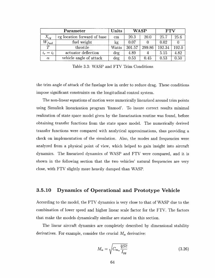
Parameter Units WASP FTVXcg cg location forward of base cm 20.3 20.0 25.7 25.6
Wfuel fuel weight kg 0.07 0 0.02 0T throttle Watts 301.57 299.86 192.34 192.0
Zr = il actuator deflection deg 4.89 4 5.15 4.82a vehicle angle of attack deg 0.53 0.45 0.53 0.50
Table 3.3: WASP and FTV Trim Conditions
the trim angle of attack of the fuselage low in order to reduce drag. These conditions
impose significant constraints on the longitudinal control system.
The non-linear equations of motion were numerically linearized around trim points
using Simulink linearization program 'linmod'. To insure correct results minimal
realization of state space model given by the linearization routine was found, before
obtaining transfer functions from the state space model. The numerically derived
transfer functions were compared with analytical approximations, thus providing a
check on implementation of the simulation. Also, the modes and frequencies were
analyzed from a physical point of view, which helped to gain insight into aircraft
dynamics. The linearized dynamics of WASP and FTV were compared, and it is
shown in the following section that the two vehicles' natural frequencies are very
close, with FTV slightly more heavily damped than WASP.
3.5.10 Dynamics of Operational and Prototype Vehicle
According to the model, the FTV dynamics is very close to that of WASP due to the
combination of lower speed and higher linear scale factor for the FTV. The factors
that make the models dynamically similar are stated in this section.
The linear aircraft dynamics are completely described by dimensional stability
derivatives. For example, consider the crucial M, derivative:
M C = CmI (3.26)

Elevator to angle of attack transfer function, a(s)/se(s)
m o - --- FTV
S-20-
-40
-6010
- 2 10
1 100 101 102
Elevator to pitch rate transfer function, q(s)r/e(s)
- 0
2-20
-4010
- 10 10
0 101 10
2
co, rad/sec
Figure 3-7: Open loop WASP and FTV longitudinal dynamics
The ratio of M0 for the WASP and for the FTV is
MWASP vWASP /3YYFTVI / WASP 37.5 (1/1.28)30.092/0.11 = 0.95
MFTV - VFTV 24.8(3.27)
where i, is an inverse of scale-up factor for FTV. Thus inertia tensor elements provide
some freedom in tuning the dynamics of FTV by appropriately distributing some of
its mass. Figure 3-7 shows the comparison of longitudinal WASP and FTV dynamics
for the most forward cg location in both vehicles. It can be seen that short period
frequencies are closely matched while the phugoid frequency of FTV is larger since
it flies slower, which is consistent with the phugoid approximation. Both transfer
functions are minimum-phase, thus magnitude plots convey all pertinent information.
The FTV dutch roll and spiral modes are close to those of WASP, because of the
same kind of scaling reasons described above for the longitudinal dynamics. The roll
subsidence pole, however, is significantly faster for FTV, because the FTV's wings
are made of carbon fiber, and are considerably lighter than the WASP wings, which
are aluminum. Rolling inertia of WASP is three times larger than for the FTV. The
important modes for lateral stability are dutch roll and spiral, thus FTV fulfills its
purpose of simulating WASP dynamics in terms of these modes. Figure 3-8 shows

Rudder to sideslip angle P(s)/Sr(s) Rudder to yaw rate r(s)/,r(s)
0 100
-50 0 I
5-oo -oo
M-150 a-200 200
.0 .- 300a -250
-300 -400
-350 -500102 100 102 o102 100 10
(o, rad/sec o), rad/sec
Figure 3-8: WASP and FTV open loop lateral dynamics
transfer functions from rudder (i.e. differential stabilizer deflection) to yaw rate and
sideslip angle for WASP and FTV. The discrepancy in the phase plot of r(s)/Sr(s)
transfer function is a numerical artifact, caused by 360 degrees phase wraparound.
3.6 Control System Design
3.6.1 Goals and Challenges
Gust disturbance versus inertial attitude stiffness
For a small aircraft control system the major challenge is design to accomodate gust
disturbances. Vertical and side gusts are only an order of magnitude smaller than
the speed of the vehicle, thus a and 4 responses to gusts are severe. To make a
gust rejection control system, the natural ability of aircraft to turn itself into the
wind (weathercock stability) must be augmented. Thus, the goal is to keep aircraft
attitude, with respect to wind axes, constant. For surveillance purposes it is desirable
to keep aircraft attitude with respect to inertial space fixed. These goals obviously
contradict each other, and a reasonable trade off must be achieved. The first priority
for any aircraft is a stable flight, so it may be necessary to use an actively controlled
gimbal system to stabilize the camera.
Surface allocation
For both WASP and FTV, large angle of attack responses to vertical gust inputs
are prohibitive, because they cause the vehicles to fly in a near-stall regime. FTV
is designed to fly slower and is more vulnerable to gusts than WASP. The vehicles
do not have ailerons, thus there are only two independent control effectors to con-
trol longitudinal, lateral and directional control variables. It is natural to decouple
the longitudinal channel from lateral and directional by considering only symmetric
and antisymmetric actuator inputs. Thus, "elevator" and "rudder" commands are
calculated and then allocated to physical surfaces:
6e = 2zr+ 6T r- (3.28)2 2
3.6.2 Prototype Vehicle Command Augmentation System
(CAS)
Longitudinal CAS
The choice of a longitudinal control variable depends on the pilot's perception of the
vehicle's motion, i.e. the variable that the pilot observes. The prototype vehicle is
a remotely piloted aircraft, and the pilot observes the vehicle from the ground. It is
assumed that the pilot observes flight path angle, which for a small angle of attack is
close to pitch attitude. Unless the vehicle is very agile, the pilot prefers to command
the rate of the state, not the state itself. For a highly maneuverable RC aircraft,
a pilot might prefer controlling pitch attitude directly. FTV is a sluggish aircraft,
thus pitch rate was chosen as the longitudinal control variable. Another reason for
this choice is turn entry, for which the appropriate non-zero pitch rate should be
commanded.
Phasor diagrams for the short period and phugoid mode of WASP are shown in
Figure 3-9 and Figure 3-10. These diagrams correspond to the trim condition with

Short period, on = 2.5 r = 0.46
08-
06
0.4
02
0
-0 2
-0 4
-0.6
-0 8
-1
-1 -08 -0.6 -04 -02 0 02 0.4 0.6 08 1
Figure 3-9: Short period phasor diagram
the fuel tank full. In the longitudinal phasor diagrams, the component corresponding
to forward velocity was divided by the trim value Uo to have non-dimensional scaling,
so as to be consistent with other variables. As can be seen, the modes are consistent
with traditional trends for aircraft: the short period dynamics are concentrated in
pitch rate q, angle of attack a, and pitch angle 0, with almost no effect on forward
velocity. Similarly, the phugoid dynamics are exhibited in pitch, forward velocity and
pitch rate, with almost no contribution to angle of attack.
The light damping (( = 0.26) of the short period mode can be accounted for by
the small tail area and short moment arm between c.g. and tail surfaces. The natural
frequencies of phugoid and short period are separated by less than a decade. This can
be explained using phugoid and short period approximations. The phugoid frequency
can be approximated as
W2Cm CL (3.29)\2 Cm1qCLa + 2mCma/(pS)
For WASP, which is a slow and heavy vehicle, the second term in the denominator,
containing mass, dominates, and the following approximation can be used:

Phugold, (on = 0.51 = 0.064
08-
06
0.4
02 -
0-
-0 2
-0.4
-0.6
-0 8
-1
-1 -08 -0.6 -04 -02 0 02 04 06 08 1
Figure 3-10: Phugoid phasor diagram
wn = = PSCL (3.30)m
Substituting for lift coefficient at level flight CL = m/(qS), yields a simple approxi-
mation for phugoid frequency:
wn = g (3.31)
VT
For the nominal FTV model, Equation 3.31 yields a phugoid frequency of 0.5 rad/sec.
This approximation shows that phugoid frequency depends mainly on airspeed. On
the other hand, natural frequency for short period approximation is
ns, = - M, (3.32)
The M, term dominates in the above expression for WASP and it can be further
simplified to
M , C S (3.33)
Since vehicle velocity VT is relatively small, and pitching inertia Iy, is relatively
69
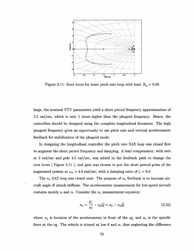
S ... .. ... .. .... .":" ; ~ ..... "........ ..'. ........... :
2 . .. ....... ....... ....... "... .. ..... .
-3 ." . -" : ":
-3 -2.5 -2 -1.5 -1 -05 0Real Axis
Figure 3-11: Root locus for inner pitch rate loop with lead, Kq = 0.06
large, the nominal FTV parameters yield a short period frequency approximation of
2.5 rad/sec, which is only 5 times higher than the phugoid frequency. Hence, the
controllers should be designed using the complete longitudinal dynamics. The high
phugoid frequency gives an opportunity to use pitch rate and vertical accelerometer
feedback for stabilization of the phugoid mode.
In designing the longitudinal controller the pitch rate SAS loop was closed first
to augment the short period frequency and damping. A lead compensator, with zero
at 3 rad/sec and pole 4.5 rad/sec, was added in the feedback path to change the
root locus ( Figure 3-11 ), and gain was chosen to put the short period poles of the
augmented system at w,, = 4.0 rad/sec, with a damping ratio of ( = 0.8.
The n, SAS loop was closed next. The purpose of nz feedback is to increase air-
craft angle of attack stiffness. The accelerometer measurement for low-speed aircraft
contains mostly u and a. Consider the nz measurement equation:
nz = z- _xaQ az - aQ (3.34)m
where Xa is location of the accelerometer in front of the cg, and a, is the specific
force at the cg. The vehicle is trimed at low 0 and a, thus neglecting the difference
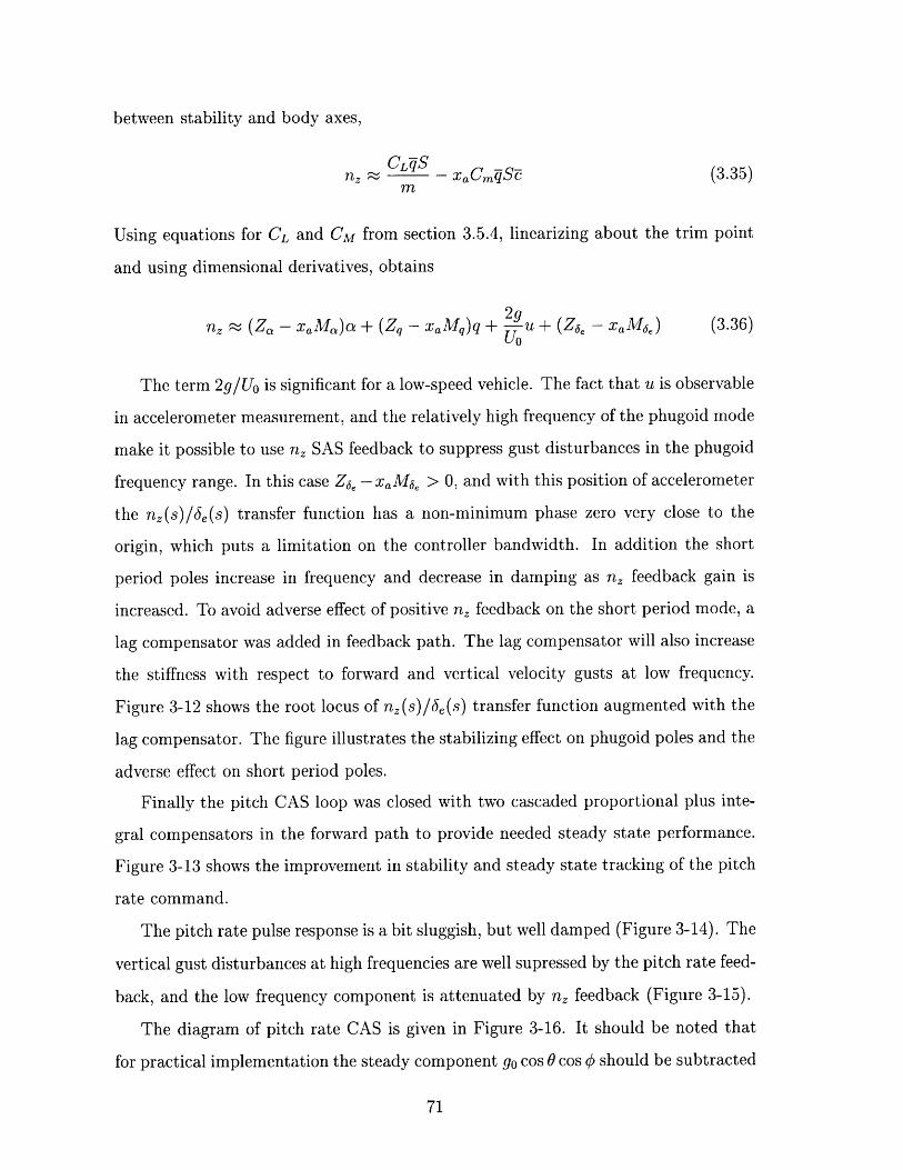
between stability and body axes,
n z , - xCm-qS- (3.35)m
Using equations for CL and CM from section 3.5.4, linearizing about the trim point
and using dimensional derivatives, obtains
nz e (Z - xaMo)a + (Zq - xaMq)q + 2u + (Z 6e - xaM3 e) (3.36)
The term 2g/Uo is significant for a low-speed vehicle. The fact that u is observable
in accelerometer measurement, and the relatively high frequency of the phugoid mode
make it possible to use nz SAS feedback to suppress gust disturbances in the phugoid
frequency range. In this case ZJ - XaMe > 0, and with this position of accelerometer
the nz(s)/ 6 e(s) transfer function has a non-minimum phase zero very close to the
origin, which puts a limitation on the controller bandwidth. In addition the short
period poles increase in frequency and decrease in damping as nz feedback gain is
increased. To avoid adverse effect of positive nz feedback on the short period mode, a
lag compensator was added in feedback path. The lag compensator will also increase
the stiffness with respect to forward and vertical velocity gusts at low frequency.
Figure 3-12 shows the root locus of nz(s)/6e(s) transfer function augmented with the
lag compensator. The figure illustrates the stabilizing effect on phugoid poles and the
adverse effect on short period poles.
Finally the pitch CAS loop was closed with two cascaded proportional plus inte-
gral compensators in the forward path to provide needed steady state performance.
Figure 3-13 shows the improvement in stability and steady state tracking of the pitch
rate command.
The pitch rate pulse response is a bit sluggish, but well damped (Figure 3-14). The
vertical gust disturbances at high frequencies are well supressed by the pitch rate feed-
back, and the low frequency component is attenuated by nz feedback (Figure 3-15).
The diagram of pitch rate CAS is given in Figure 3-16. It should be noted that
for practical implementation the steady component go cos 0 cos q should be subtracted

3 04
032
0 0 .0 0 ea. .i
Flti
-3 -0.4 ". "' " :
-6 -4 -2 0 -0.6 -0.4 -0.2 0Real Axis Real Axis
Figure 3-12: Root locus for nz/1e(s) transfer function with lag, Knz = 0.015
q(s)/qc(s)
-10 '2 -.2.00!i . ..... ... .. ... ..... i i i i
-200 Closed loopS .... .... .--- Loop transmission
-- - Open loop-400......
. . . ......
-00010
-2 10 10 10, 1(
f, radIsec
Figure 3-13: Open loop, closed loop and loop transmission for q(s)/qcmd(s) transferfunction
72

2 4
15 3
S1 "2
05 1
0 00 2 4 6 8 10 0 2 4 6 8 10
15 025
02
(015
S6 01
0 005
-05 00 2 4 6 8 10 0 2 4 6 8 10
time, sec time, sec
Figure 3-14: Pitch rate pulse response with CAS-on
1
0
d -2 1
-3 lit
-4 U Po
-5 -1
2 04 2
-30246810 -042468100 2 4 6 8 10 0 2 4 6 8 10
time, sec time, sec
Figure 3-15: Vertical gust response with CAS-on
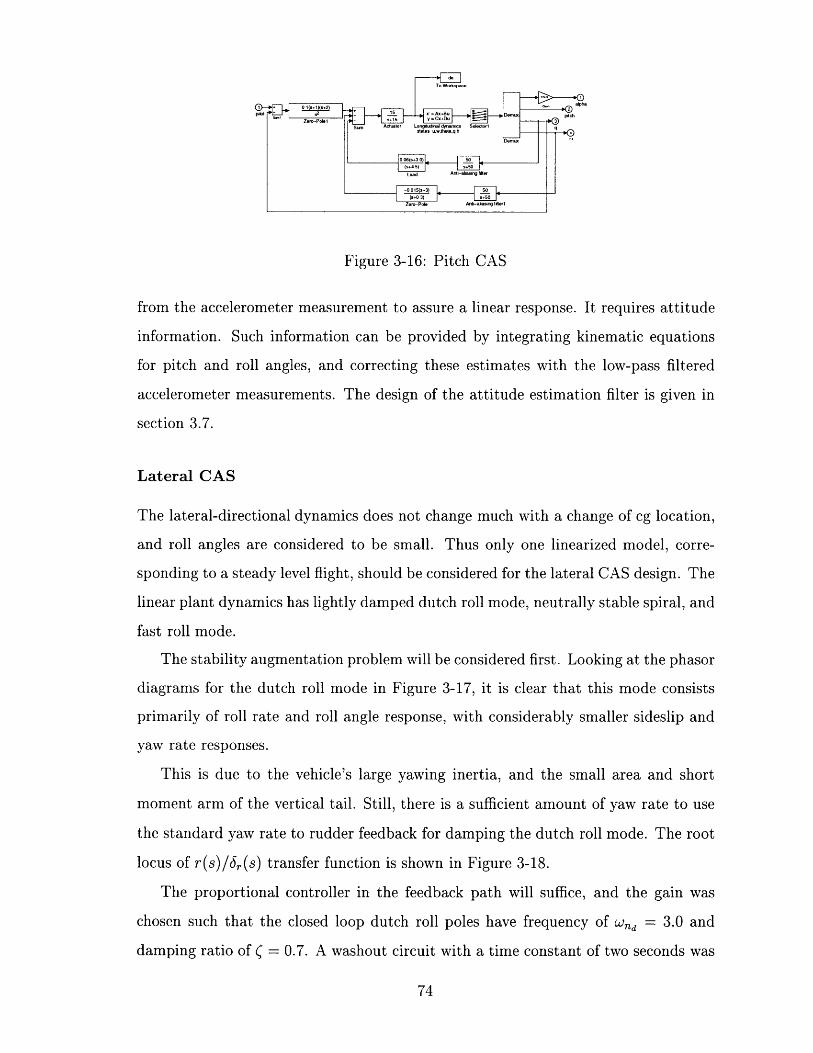
Figure 3-16: Pitch CAS
from the accelerometer measurement to assure a linear response. It requires attitude
information. Such information can be provided by integrating kinematic equations
for pitch and roll angles, and correcting these estimates with the low-pass filtered
accelerometer measurements. The design of the attitude estimation filter is given in
section 3.7.
Lateral CAS
The lateral-directional dynamics does not change much with a change of cg location,
and roll angles are considered to be small. Thus only one linearized model, corre-
sponding to a steady level flight, should be considered for the lateral CAS design. The
linear plant dynamics has lightly damped dutch roll mode, neutrally stable spiral, and
fast roll mode.
The stability augmentation problem will be considered first. Looking at the phasor
diagrams for the dutch roll mode in Figure 3-17, it is clear that this mode consists
primarily of roll rate and roll angle response, with considerably smaller sideslip and
yaw rate responses.
This is due to the vehicle's large yawing inertia, and the small area and short
moment arm of the vertical tail. Still, there is a sufficient amount of yaw rate to use
the standard yaw rate to rudder feedback for damping the dutch roll mode. The root
locus of r(s)/6r(s) transfer function is shown in Figure 3-18.
The proportional controller in the feedback path will suffice, and the gain was
chosen such that the closed loop dutch roll poles have frequency of Wnd = 3.0 and
damping ratio of ( = 0.7. A washout circuit with a time constant of two seconds was

Dutch roll, o n = 3.9 r = 0.18
R
.. .I .
-1 -0.8 -0.6 -0.4 -0.2 0 02 0.4 0.6 0.8 1
Figure 3-17: Dutch roll phasor diagram for the FTV
4 -
C r. f-1
-3-
-4.5 -4 -3.5 -3 -2.5 -2 -1.5 -1 -0.5 0Real Axis
Figure 3-18: Root locus for r(s)/6,(s) transfer function, K, = 1.3
75
...... ......
. . . .... ......
. ..... . ...
. ......... .
... ..............
I II
i
I I
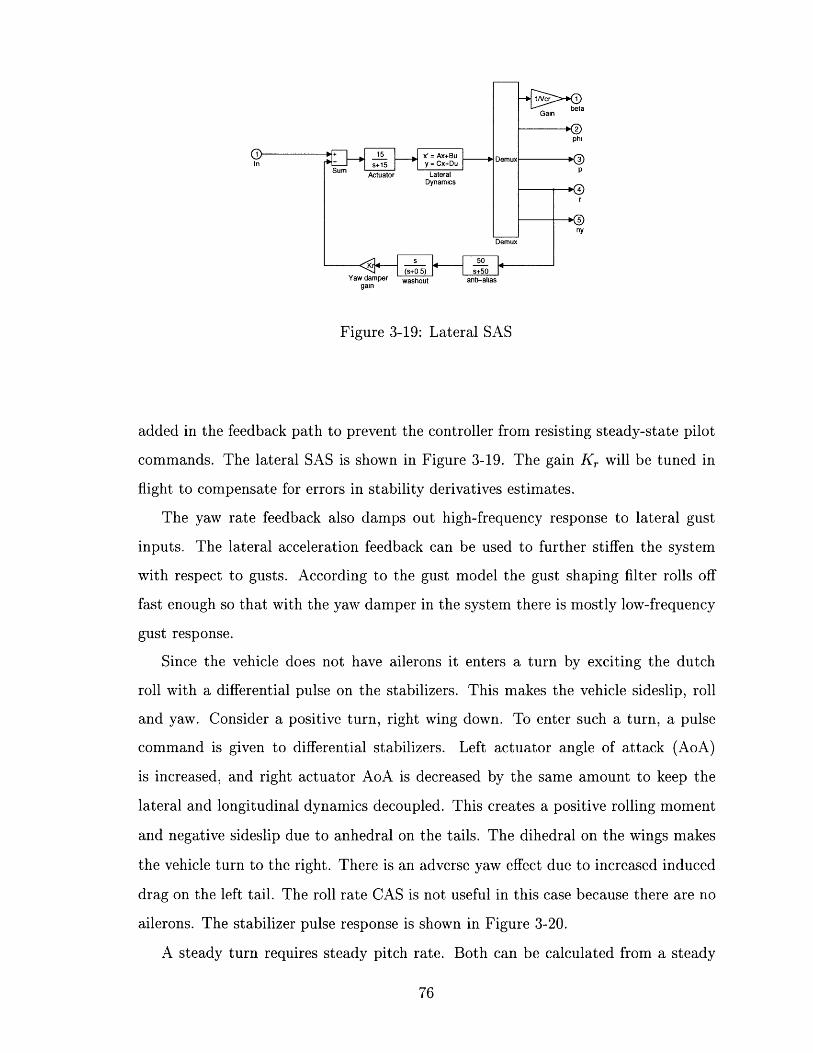
gain
Figure 3-19: Lateral SAS
added in the feedback path to prevent the controller from resisting steady-state pilot
commands. The lateral SAS is shown in Figure 3-19. The gain Kr will be tuned in
flight to compensate for errors in stability derivatives estimates.
The yaw rate feedback also damps out high-frequency response to lateral gust
inputs. The lateral acceleration feedback can be used to further stiffen the system
with respect to gusts. According to the gust model the gust shaping filter rolls off
fast enough so that with the yaw damper in the system there is mostly low-frequency
gust response.
Since the vehicle does not have ailerons it enters a turn by exciting the dutch
roll with a differential pulse on the stabilizers. This makes the vehicle sideslip, roll
and yaw. Consider a positive turn, right wing down. To enter such a turn, a pulse
command is given to differential stabilizers. Left actuator angle of attack (AoA)
is increased, and right actuator AoA is decreased by the same amount to keep the
lateral and longitudinal dynamics decoupled. This creates a positive rolling moment
and negative sideslip due to anhedral on the tails. The dihedral on the wings makes
the vehicle turn to the right. There is an adverse yaw effect due to increased induced
drag on the left tail. The roll rate CAS is not useful in this case because there are no
ailerons. The stabilizer pulse response is shown in Figure 3-20.
A steady turn requires steady pitch rate. Both can be calculated from a steady

2
0
0
C-0.02
0 2 4 6time, sec
20
10
5
8 10 0
8 10
,10
5
02 4 6
time, sec8 10
Figure 3-20: Differential stabilizer pulse response
state load factor, or roll angle ( [28, vol. 1, page 226]):
VT
n = L/W = 1/cos
Q = gtanosin _ g n -
VT VT
turn rate
load factor
pitch rate
yaw rate
The roll angle is available from the attitude determination system (Section 3.7). This
estimate should be low pass filtered, and the corresponding pitch rate fed as an input
into the pitch rate command channel. The low pass filter time constant should be
chosen in such a way that the roll angle (5) crossfeed does not affect stability, and
at the same time the turn entry is fast enough. This constant can also be tuned in
flight.
-z'0 2 4 6 8 11
20
10
0-
8 102 4 6
2 4 60 2 4 6 8 10
(3.37)
a.
n
tm3
r so. . .
0
3.7 Navigation and Attitude Determination Sys-
tems
3.7.1 Gravity Aiding with Strapdown Sensors
Gravity aiding is an attitude determination method that employs angular rate and
translational acceleration information from a strapdown IMU. Most small UAVs are
equipped with strapdown, as opposed to gimballed, IMUs. The gravity aiding ap-
proach was used for the prototype vehicle. When the IMU is used in a stand alone
mode the gravity aiding is the only way to provide attitude information needed for
autopilots. Other applications may include a backup vertical determination system,
which is run in parallel with a master system, and provides accurate attitude infor-
mation for flight stabilization in case of failures of other sensors. For example an
unmanned helicopter considered in Chapter 2 has an extended Kalman filter (EKF)
as a master filter, which uses GPS, IMU, compass and sonar measurements. In case of
loss of GPS track, the attitude estimate will diverge unless frequency characteristics
of sensor models are taken into account in EKF design. The system may temporarily
switch to a gravity aiding estimator, engage pitch attitude hold and bank angle hold
autopilots, and maintain steady level or hovering flight until GPS is reacquired.
The approach uses the same idea as a vertical gyro in a regular aircraft, in which
a restoring torque, proportional to accelerometer measurements, is used to correct
the low frequency gyro drifts. In case of a strapdown unit, the role of the vertical
gyro is played by a set of three rate gyros with orthogonal axes. The angular rate
measurements are used in the attitude kinematic equations to solve for Euler angles.
This provides high-bandwidth attitude information. The gyros have drifts, and the
low pass filtered accelerometer measurements are used to correct for them. The low
pass filter time constant should be big enough to filter out the vehicle dynamics from
accelerometer measurements.
Frequency and time domain design approaches for the gravity aiding attitude
reference system are considered in [4]. The time domain design is based on an EKF.
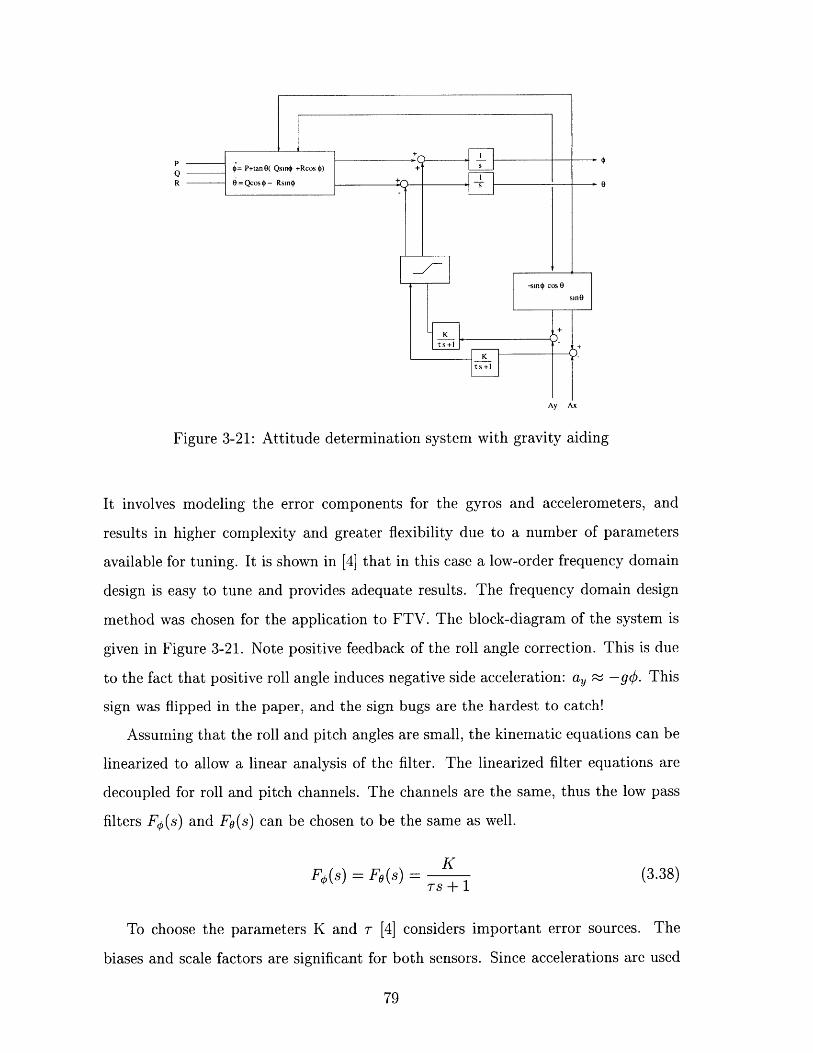
= P+tan ( Qsin +Rcos ) + s
R -- e6 = Qcos - RsinO
-sm cos 0
_/--smn
IS+1
Ay Ax
Figure 3-21: Attitude determination system with gravity aiding
It involves modeling the error components for the gyros and accelerometers, and
results in higher complexity and greater flexibility due to a number of parameters
available for tuning. It is shown in [4] that in this case a low-order frequency domain
design is easy to tune and provides adequate results. The frequency domain design
method was chosen for the application to FTV. The block-diagram of the system is
given in Figure 3-21. Note positive feedback of the roll angle correction. This is due
to the fact that positive roll angle induces negative side acceleration: a, _ -go. This
sign was flipped in the paper, and the sign bugs are the hardest to catch!
Assuming that the roll and pitch angles are small, the kinematic equations can be
linearized to allow a linear analysis of the filter. The linearized filter equations are
decoupled for roll and pitch channels. The channels are the same, thus the low pass
filters Fp(s) and Fo(s) can be chosen to be the same as well.
FO (s) = Fo(s) = K (3.38)TS +1
To choose the parameters K and r [4] considers important error sources. The
biases and scale factors are significant for both sensors. Since accelerations are used
only to correct for a very slowly varying gyro bias, the vehicle dynamics in the ac-
celerometer measurements is also an error source for this application. The white
noise was also added to both sets of sensors. Detailed account of error modeling for
the IMU is given in Section 3.5.7. From the linearized model analysis, the suggested
values for the low pass filter parameters are:
1T = 1 (3.39)
KK = o (3.40)
where Eg is assumed gyro bias value, and 60, is the specified target value for the steady
state pitch angle error due to o0. There is no steady state error due to initial error.
The values T and K were optimized with respect to steady state performance. This
design also guarantees -40 dB/decade slope for the transfer function from acceleration
to pitch estimate error, thus rejecting high frequency accelerometer errors. Effectively,
there is a usual trade off between high frequency noise rejection and bias rejection.
For the Crossbow IMU used in FTV the short term (100 sec) bias stability was
estimated at 0.01 deg/sec. The accelerometer bias is on the order of 5 mg, which
results in 0.3 degrees attitude error. Thus, designing for a steady state error due to
gyro bias 60, = 0.3 deg the low pass filter cutoff frequency is 0.03 rad/sec, which is
two decades below the aircraft short period frequency. This should give a sufficient
attenuation of vehicle dynamics. In case the aircraft undergoes a steady turn or
acquires significantly non-zero steady pitch attitude, the algorithm will lead to steady
state estimation error. To account for it, the amount of accelerometer feedback should
be limited to 1-2 degrees. This is analogous to the erection cutoff mechanism in a
vertical gyro, where there is a limit on the restoring torque.
The aircraft response to pulse commands in both channels was simulated, and
Figure 3-22 shows that the estimator tracks high frequency dynamics due to pulse
inputs, and the accelerometers correct long term drifts due to gyro biases. This is
conspicuously seen in the pitch response in this case.

1 0-- True angleI- Estimate
5-
00 10 20 30 40 50 60 70 80 90 100
4
2
1 . . ..
0
0 10 20 30 40 50 60 70 80 90 100time, sec
Figure 3-22: Gravity aiding algorithm performance
3.7.2 Velocity Matching
GPS information can also be used for attitude determination. The idea of the velocity
matching algorithm is to compare INS computed velocity with the velocity measured
by GPS, and extract attitude information from the comparison. The method can
be employed in the operational WASP system for an in-flight attitude and heading
angles determination.
The velocity matching method uses linearized error equations, thus initial rough
estimate of vehicle's attitude is needed. To provide this estimate, GPS-only algorithm
for attitude determination is used. Assume that the aircraft angle of attack and angle
of sideslip are small, then the heading and pitch angle can be determined from GPS
velocity information, which gives information on flight path angle. Single antenna
GPS receiver was used for roll angle determination in [21]. The algorithm is based on
the derivation of inertial acceleration of the vehicle from the GPS velocity information
by using the third-order Kalman filters. This GPS-only alignment technique will
provide up to several degrees accuracy in all axes in less than 5 sec. Then GPS
velocity matching can be used to assure fine alignment.
Design guidelines for velocity matching method are given in [34]. Non-linear INS
equations are initialized with GPS-derived position, velocity and attitude. Velocity
and attitude satisfy:
" = Cnfb - [2w!' + w n ] x vX + g (3.41)n (3.41)
=b Cb nb
where
v - vehicle velocity with respect to Earth in NED frame
Cbn - transformation matrix from body frame to NED frame
fb - accelerometer measurements
iw - Earth angular rate in NED frame
wn - NED frame angular rate relative to Earth-fixed axis in NED frame
At a nominal WASP velocity of 50 m/s, 11 [2w~ + wn ] x v n |< 0.3 mg. This is below
accelerometer bias, thus these terms can be omitted. Then the linearized INS error
equations are used to design a Kalman filter. It is important to model the gyro biases
as states of Kalman filter. This "tells" the filter that the low frequency information
from the gyros is biased, and the filter should assign more weight to the GPS and
accelerometer measurements at low frequencies. In this sense the KF is similar to
the kind of complementary filter approach employed in design of the gravity aiding
algorithm of Section 3.7.1. Dynamic driving noise due to accelerometer and gyro high-
frequency errors should be modeled as well. This noise is relatively small compared
to the high frequency noise of GPS, but the introduction of the dynamic driving
noise eliminates possible singularity in the covariance matrix. For applications where
pre-calibration of the accelerometers is impossible, such as aerial deployment after
gun launch, the accelerometer bias states should be included in the filter to achieve
in-flight calibration. The biases are modeled as first order Markov processes with a
large time constant. If the time constant for the bias term is much larger than the
mission time, they can be modeled as random constants.
The filter design is given below. Let Cb be a transformation matrix from local
NED frame into body frame, so that for any vector : (n = Cb. Define Cn
[I - I] Cbn - current estimate of transformation matrix. I is a small angle rotation
matrix:
0 -6y 6P
-y 0 -6
-6I 6a 0
where 6a, 6S, 6y attitude errors. The linearized error equations for attitude states
are:
= - win, x - Cbnb - Cbng (3.42)
where0 - attitude error
wn - NED frame rate
wb - gyro biases
(9 - gyro noise
Because the vehicle is moving slowly, wn f1 14 deg/hr, which is below the
MMISA sensor drifts, angular rate of the NED frame can be neglected. The ac-
celerometers and GPS will be the primary sensors providing the low-frequency atti-
tude information. Thus the attitude error equation can be reduced to:
= -CbnWb (3.43)
The error equations for velocity states are:
6iv = fn x P + Cbnab + Cb a (3.44)
where
fn - accelerometer measurements resolved in NED frame
ab - accelerometer biases
6v - north and east velocity errors in NED frame
a - accelerometer noise
The equations for bias states are
db= 0 b=0 (3.45)
Thus, Kalman filter states are:
6 [ = I 6 a 60 67 6V, 6Vn Wbx Wby Wbz abx aby abz
The dynamic equations are 3.43, 3.44 and 3.45, which should be represented in
a matrix form for KF solution. A diagonal 11 x 11 covariance matrix, for dynamic
driving noise, should be built using specifications for gyro noise and accelerometer
noise.
The measurement equations are
VeINS - VeGPS 6Vne Ti
VINS - VGPS vn) T]
where q is the GPS velocity measurement noise. The noise covariance is R = or 2x2.
For P(Y) code, a. = 0.01 m/s. An initial error covariance matrix is determined
by ambiguity in initial estimates of corresponding states. Then a continuous time
KF model is discretized and split into measurement update and time propagation
equations. The simulation shows that the pitch and roll angle estimate convergence
is dependent primarily on the accelerometer biases. To estimate the yaw angle, the
aircraft has to make a lateral-directional maneuver to excite error dynamics, so that
it becomes observable in the inertial velocity measurements. To make this point clear,
consider scalar form of 3.44.
6 VN = - fD/ 3 + fE57 + abN (3.46)
6 VE = fDa - fN 6 7 + abE
If the aircraft is flying straight and level, the apparent acceleration vector is aligned
with down axis in NED frame: fE = 0 and fN = 0, hence -y becomes unobservable
in the velocity measurement. To make heading error observable, a lateral-directional
maneuver is needed. In the example, given in [34], a .1 g weave maneuver with 10
deg/hr gyro bias and 2 mg accelerometer bias results in subdegree level accuracy in
all three axis. The gust disturbances may be sufficient to excite error dynamics, then
no maneuver is needed to guarantee convergence.
3.7.3 Navigation System for Operational Vehicle
A standard EKF for navigation is suggested, using the IMU as a master sensor and
GPS position and velocity information for measurement updates. Depending on the
quality of micromechanical inertial sensors, various error sources should be modeled.
As it currently exists, scale factor errors and short term biases should be modeled
for both gyros and accelerometers. A standard tightly coupled INS/GPS system
was used as a single source of navigation and attitude information in several guided
munitions programs in Draper Laboratory. The unmanned helicopters developed at
Draper Laboratory and MIT also use EKF, using additional sensors. The detailed
design of an EKF for the unmanned helicopter navigation and attitude determination
is considered in Section 2.3.

86

Chapter 4
Conclusion
In the process of development of the avionics systems for two small unmanned aircraft,
many lessons in system integration, modeling, simulation and algorithms were learned.
These will be used in future designs of unmanned aircraft.
In hardware, the improvements in performance and cost can be achieved by fore-
seeing the common problems for small UAVs in the preliminary design phase, and
by using the experience gained to mitigate the adverse effects. These include sensor
degradation due to vibration, electromagnetic (EM) noise, effects of EM interference
on ranges of remote control and communication links.
Fast computers and data acquisition systems allow better modelling of errors in
estimation filters. This places less stringent requirements on sensor performance. A
set of attitude determination and navigation algorithms have been tested in simulation
and in the field, and important sensor errors were identified or predicted.
A model for a low speed gun-launched surveillance aircraft was developed and
analyzed. A control augmentation system for a prototype vehicle was designed and
tested with the pilot-in-the-loop simulation. A classical design approach was taken to
develop an intuitive feeling for a physically sound choice of the control variables and
feedbacks. The problem of gust disturbance rejection for a low speed vehicle can be
effectively addressed by using the modern control methods, along with the knowledge
gained from the model analysis and classical design. A reasonable choice would be to
use a design approach that allows frequency weighting of desired outputs, and simul-

taneously incorporates ambiguity in the estimates of aircraft parameters, especially
the lateral-directional control and damping derivatives. New software packages for
real p synthesis [22], [12] allow to account for available information on gust frequency
content and uncertainty in aerodynamic derivatives. This tool also allows one to ob-
tain boundaries for performance, which will provide limitations on product use. This
determines whether the UAV can be used in a certain application. The algorithm
performance is degraded with the increasing number of uncertain parameters, thus
the careful analysis of the model helps identify the most important ones.
The field of small UAVs is growing rapidly, and the work on these two projects
during the past two years has been challenging. A great number of improvements
can be made in these systems, and new designs will contribute to the exciting area
of unmanned aircraft.
Appendix A
Nonlinear Model in Simulink
A.1 Block Hierarchy
The model is built using a hierarchy of Subsystem blocks. At the lowest level there are
two S-functions 'aero.m' and 'eqmotlO.m' which contain computation of aerodynamic
forces and moments, and aircraft 6-DOF equations of motion correspondingly, and
an engine model Subsystem block. At the higher level of hierarchy the actuator block
provides inputs to the aircraft block, and sensor block takes inputs from the a/c block.
There are two sets of these blocks. One is a fully linear (except non-hard actuator
deflection limiters) and analog, which is used for the linearization. The other includes
the sensor and actuator non-linearities, sensor noise and quantization. At the highest
level are the trim inputs, pilot inputs and control augmentation system. All three
levels in this hierarchy are presented in Figures A-1 - A-3.
The simulation is initialized from Matlab workspace. The simulation parameters
are passed to Simulink blocks and S-functions automatically. The inputs to the
simulation are defined in workspace. The simulation is run using 'sim' command
with a vector of inputs and a time vector.

WASP Simulation Framework
Figure A-1: Simulation. Level 1: I/O
Nonlinear WASP Model
elevator cmdght stab
rudder crmd left stab!-
throttle cmd throttle
Actuators
U
Vright stabilizer W
phi
theta
psi
left stabilizer P
Q
R
H
fxthrottle
ly
tz
waspl0
Selector
Accel X
Accel Y
AccelZ
fxty fz P RRoll gyro
Pitch gyro
Yaw gyrc
Sensors
Selector Xout
Selectori To Workspace
Clock To Workspacel
Figure A-2: Simulation. Level 2: sensors and actuators
90
OutMux
Mux1
Inl
In2
In3

10-state WASP dynamic model for trim analysis
Figure A-3: Simulation. Level 3: equations of motion
A.2 C-MEX vs M files
The user-defined S-function blocks can be written as either M-files or so called C-MEX
files. The C-MEX files are just the C language source code files, written according
to certain simple rules. Using the M-file S-functions is slow compared to the C-MEX
S-functions. Even for a relatively low-order simulation like WASP's, it is worth using
the C-MEX functions. If one is going to use the Simulink simulation with animation
output or with human operator external input, then C-MEX implementation is a
must.
A.3 Animated Pilot-in-the-Loop Simulation
In the development of the prototype vehicle two versions of animated simulation were
used extensively for control system design and for pilot training. For the design of
control system, the Simulink based simulation was converted to C-MEX files, and
connected to simplified animation program and to the RC receiver interface. The
animation was based on OpenGL graphics package, it featured the rigid body vehicle

dynamics, terrain with a grid and the vehicle shadow when altitude is low. This is a
minimum requirement for a realistic pilot perception. The animation program takes
vehicle attitude and position as inputs. It can be also used for post flight analysis of
the flight using recorded data. The receiver interface, described in Section 2.2 commu-
nicated with the host computer via serial interface to provide pilot commands. This
setup allows rapid prototyping of control systems, using standard Simulink libraries.
The animation of the WASP vehicle was done in Draper Laboratory, the interfaces
between Simulink and the animation and the receiver interface were provided by
Emilio Frazzoli, a graduate student at MIT.
For pilot training a Silicon Graphics workstation-based simulation with realistic
terrain and detailed graphics of the vehicle was used. This tool is written in C-
language, and uses SGI Graphic Libraries for animation. The same receiver interface
was used for pilot command inputs.
A.4 Suggested Framework for Hardware-in-the-
Loop Simulation
Adding hardware-in-the-loop capability to the simulation greatly reduces time for
debugging the real time code. Using the onboard CPU in the simulation with exactly
the same interfaces and timing can be easily done, if all the onboard I/O is easy to
emulate. A possible simulation framework for the FTV is given in Figure A-4.
This framework can be extended for any other sensors having serial outputs. In
case the sensor I/O is analog, the emulation of the interface and timing may become
quite complicated (it is routinely done in the industry for large scale products). For
rapid prototyping with COTS elements the use of this architecture will allow designers
to concentrate on the research, and spend less time on device drivers and debugging
the real-time software.
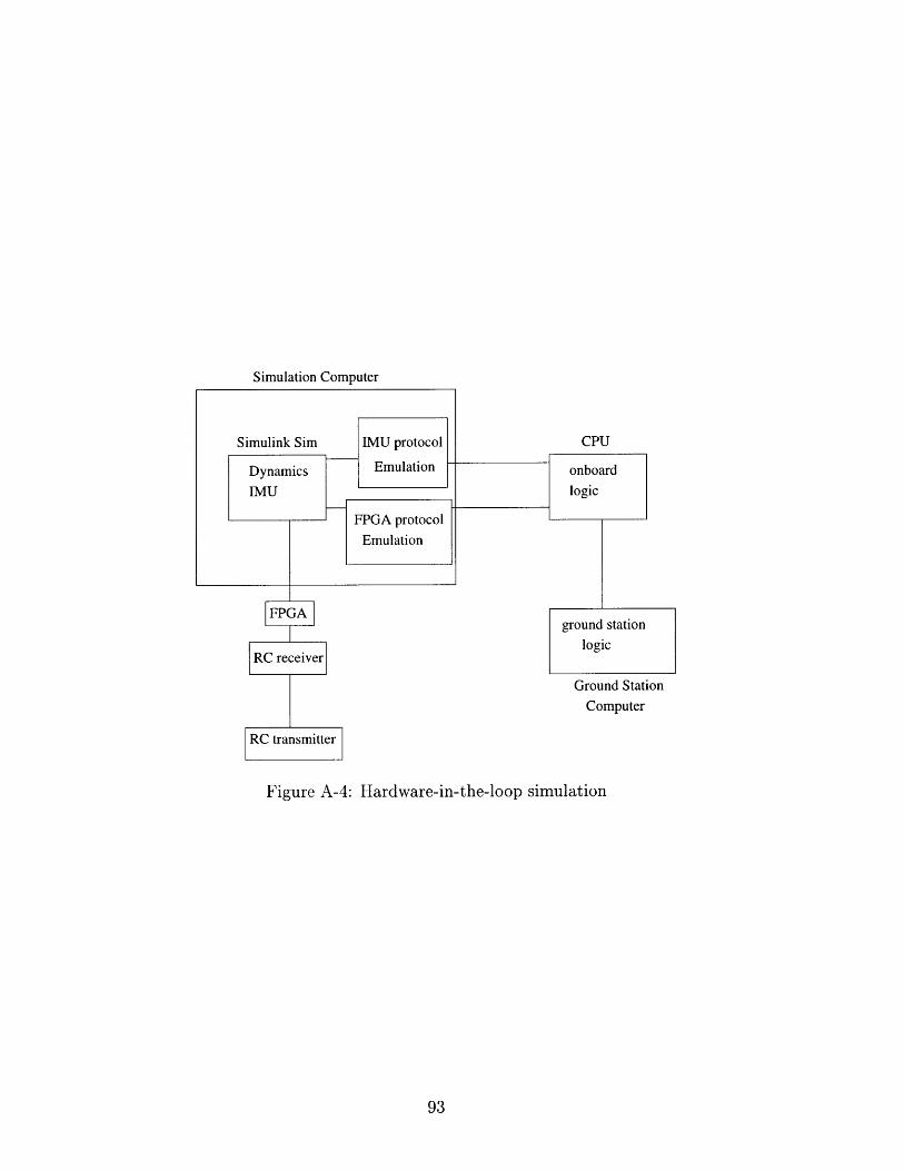
Simulation Computer
CPU
Ground Station
Computer
Figure A-4: Hardware-in-the-loop simulation

94

Appendix B
Additional Data for Navigation
Filter
B.1 Linear Propagation Matrix
Jacobian matrix from equation 2.8 can be represented in the following block way:
0 APV Apq O 0
0 AV Avq A,, Avy
0 0 Aqq 0 Aq,
0 0 0 0 0
0 0 0 0 0
where zeros stand for the zero matrices of corresponding dimensions.
partial derivatives of right hand side of equation 2.8, we shall arrive at:
Computing
(B.2)
(B.3)A,, = - 3 + ,F3
Aqq = -2 (4 - F4)
(B.1)
(B.4)
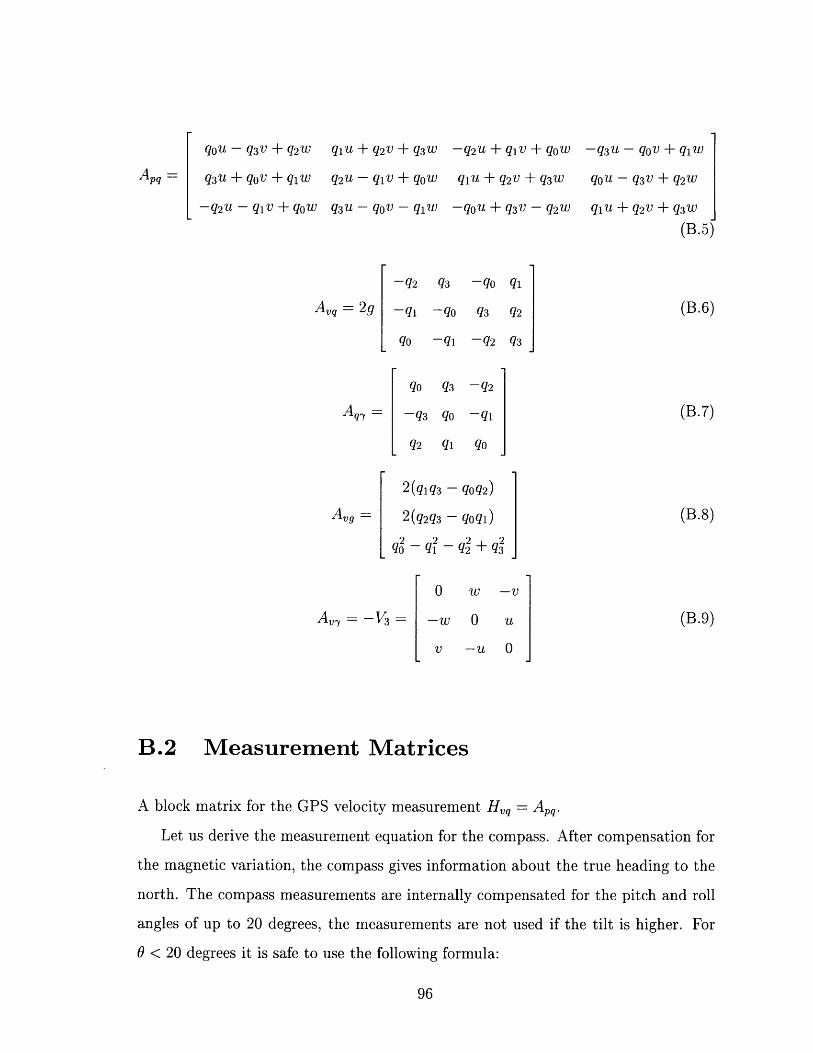
qo u - q3 v + q2 w
Apq = q3u + q0ov + qw
-q 2u - q1v + qow
qlu + q2 v + q3 w
q2 u - q1v + qo w
q3 u - q0 v - qlw
q3
-qo
-ql
-q 2 u + q1v + qow
qlu + q2 v + q3 w
-q0u + q3v - q2 w
-q 3 u - qov + ql
qou - q3 v + q2 w
q1u + q2v + q3w
(B.5)
-qo
q3
-q2
Avq = 2g (B.6)
A
q0 q3 -q 2
Aq,= -q 3 qo -q 1
q2 q1 q0
2(qiq3 - qoq 2)
vg = 2(q 2q3 - qOq1)
q2 - q2 _ q2 + q 2
0 w -
= -V 3 = -w 0
v -u
(B.7)
(B.8)
-v
-t
)
(B.9)
B.2 Measurement Matrices
A block matrix for the GPS velocity measurement Hvq = Apq,.
Let us derive the measurement equation for the compass. After compensation for
the magnetic variation, the compass gives information about the true heading to the
north. The compass measurements are internally compensated for the pitch and roll
angles of up to 20 degrees, the measurements are not used if the tilt is higher. For
0 < 20 degrees it is safe to use the following formula:
A,,v
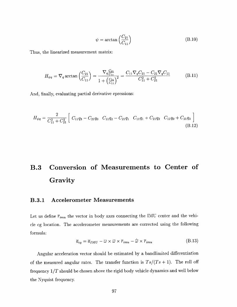
4 = arctan
Thus, the linearized measurement matrix:
C21 (B.1O)
(C 21He q Vq arctan Yc1 11 + C2)2
C1-
Cll VqC21 - C 2 1 VqCll
C11 + C 21
And, finally, evaluating partial derivative epressions:
2H, = C1 + 2
11 + C2 1
C11q3 - C 21q0 Cllql + C 21 q2C1 1 qo + C21q 3
(B.12)
B.3 Conversion of Measurements to Center of
Gravity
B.3.1 Accelerometer Measurements
Let us define imu the vector in body axes connecting the IMU center and the vehi-
cle cg location. The accelerometer measurements are corrected using the following
formula:
cg = Qf MU - a X Wj X Tim - U) X Timu (B.13)
Angular acceleration vector should be estimated by a bandlimited differentiation
of the measured angular rates. The transfer function is Ts/(Ts + 1). The roll off
frequency 1/T should be chosen above the rigid body vehicle dynamics and well below
the Nyquist frequency.
(B.11)
Cllq2 - C21q1
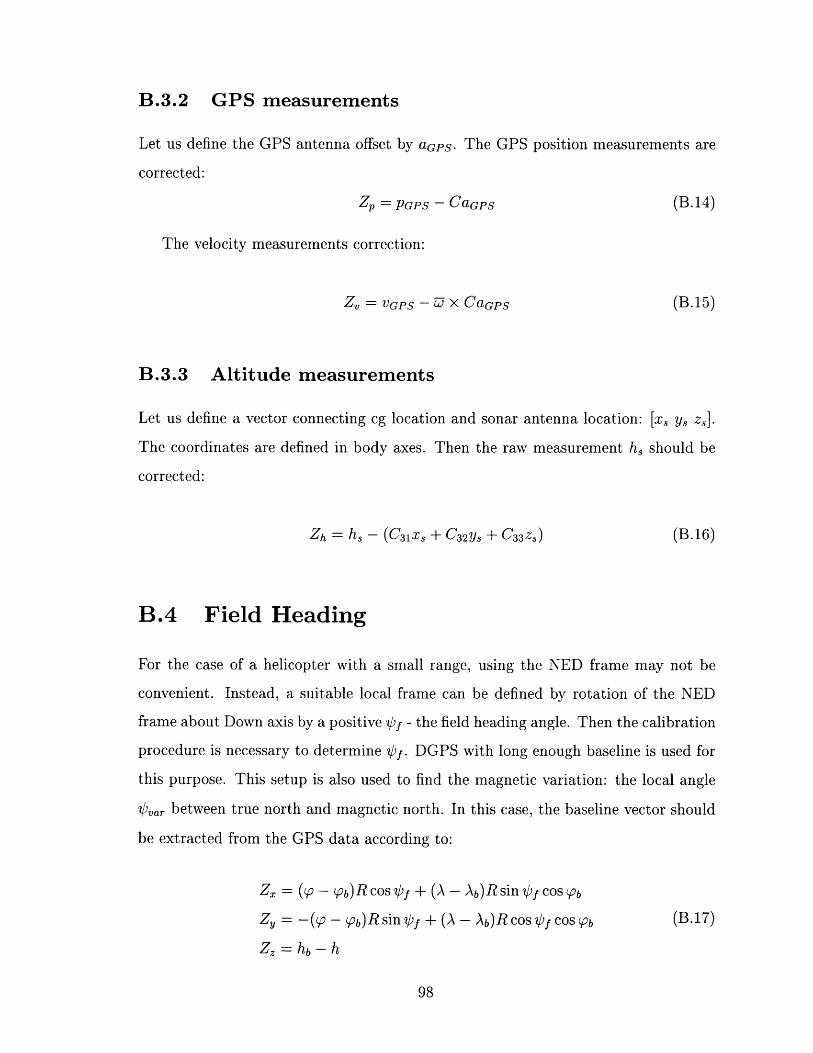
B.3.2 GPS measurements
Let us define the GPS antenna offset by aGps. The GPS position measurements are
corrected:
Zp = PGPS - CaGPS (B.14)
The velocity measurements correction:
Zv = vGPS - Z X CaGPS (B.15)
B.3.3 Altitude measurements
Let us define a vector connecting cg location and sonar antenna location: [xs ys zs].
The coordinates are defined in body axes. Then the raw measurement hs should be
corrected:
Zh = hs - (C31xs + C 32Ys + C 33zs) (B.16)
B.4 Field Heading
For the case of a helicopter with a small range, using the NED frame may not be
convenient. Instead, a suitable local frame can be defined by rotation of the NED
frame about Down axis by a positive of - the field heading angle. Then the calibration
procedure is necessary to determine of. DGPS with long enough baseline is used for
this purpose. This setup is also used to find the magnetic variation: the local angle
lvar between true north and magnetic north. In this case, the baseline vector should
be extracted from the GPS data according to:
Z = (- (Pb)R COS f + (A - Ab)R sin 'O cos pb
Z = -(Op- pb)R sin f + (A - Ab)R cos f cos pb (B.17)
Zz= hb- h

where o, A, h - latitude, longitude and altitude of the rover receiver, Pb, Ab, hb -
latitude, longitude and altitude of 'the base receiver, located at the origin of the local
frame, R - Earth radius. The values of the position and velocity covariances are then
corrected to account for of rotation.
The raw compass measurement is corrected in the following way:
Z = V - Of - Ova (B.18)

100

Bibliography
[1] Inertial Sensor Technology Trends. Guidance Technology Center, Draper Labo-
ratory, Cambridge, MA, January 1997.
[2] John D. Anderson. Fundamentals of Aerodynamics. McGraw-Hill, Inc., 1991.
[3] Michael Athans. 6.245 - Multivariable Control Systems. Lecture Notes, MIT,
1997.
[4] I.Y. Bar-Itzhack and I. Ziv. Frequency and Time Domain Designs of a Strapdown
Vertical Determination System. Guidance and Control, 1986.
[5] Arthur E. Bryson. Control of Spacecraft and Aircraft. Princeton University Press,
1993.
[6] Thierry Casiez. Compact, High-g, High Efficiency Folding Wing for a Cannon-
Launched Reconnaissance Vehicle. Master's thesis, MIT, 1998.
[7] Paul DeBitetto. Red Team Review of the Draper Small Autonomous Aerial
Vehicle. Technical report, Draper Laboratory, Cambridge, MA, May 1996.
[8] John J. Deyst. 16.840 - Real-Time Aerospace Systems. Lecture Notes, MIT,
1997.
[9] Peter Donaldson. Unmanned Vehicles Handbook. The Shephard Press, 1993-97.
[10] John R. Dowdle and Karl W. Flueckiger. An Integrated GPS/Micro-Mechanical
IMU for 5" Navy Projectiles . Guidance and Control, 1996.
101
[11] Marc Drela. 16.110 - Flight Vehicle Aerodynamics. Lecture Notes, MIT, 1997.
[12] P. M. Young et. al. Computing Bounds for the Mixed-p Problem. Intern. Journal
of Robust and Nonlinear Control, 5:573-590, 1995.
[13] Michael C. Francis. The UTA: Redefining The Air Combat System . Aerospace
America, May 1998.
[14] A. Gelb. Applied Optimal Estimation. The Analytical Sciences Corp., 1974.
[15] L.A. Gould, W.R. Markey, J.K. Roberge, and D.L. Trumper. Control Systems
Theory. unpublished, 1994.
[16] D. Gustafson and D. Lucia. Autonomous Local Vertical Determination For
Guided Artillery Shells. Presented at the ION 52nd Annual Meeting, 1996.
[17] Jean-Marc Hauss. Design of an Unmanned Aerial Vehicle. Master's thesis, MIT,
1998.
[18] Paul Horowitz and Winfield Hill. The Art of Electronics. Cambridge University
Press, 1989.
[19] Eric N. Johnson, Paul A. Debitetto, Christian A. Trott, and Michael C. Bosse.
The Draper Small Autonomous Aerial Vehicle Technical Description. Technical
report, Draper Laboratory, Cambridge, MA, 1996.
[20] Sebastien Katch. Concept Development, Mechanical Design, Manufacturing and
Experimental Testing for a Cannon Launch Reconnaissance Vehicle. Master's
thesis, MIT, 1998.
[21] Richard P. Kornfeld, R. John Hansman, and John J. Deyst. Single Antenna GPS
Based Aircraft Attitude Determination. Institute of Navigation, 1998.
[22] L. Lublin. The use of additional actuators to enhance performance robustness.
PhD thesis, MIT, 1996.
102
[23] Duane McRuer, Irving Ashkenas, and Dunstan Graham. Aircraft Dynamics and
Automatic Control. Princeton university Press, 1972.
[24] Alan V. Oppenheim and Ronald W. Schafer. Discrete-time Signal Processing.
Prentice Hall, 1989.
[25] James Paduano. 16.334 - Advanced Flight Control Systems. Lecture Notes, MIT,
1998.
[26] Richard E. Phillips and George T. Schmidt. GPS/INS Integration.
MSP Lecture Series LS-207, 1996.
[27] QNX Operating System. System Architecture.
[28] Jan Roskam. Airplane Flight Dynamics and Automatic Flight Controls. DAR-
corporation, 1995.
[29] Christopher P. Sanders, Paul A. DeBitetto, and Eric Feron. Hierarchical Control
of Small Autonomous Helicopters. Submitted to Journal of Guidance and Control,
1998.
[30] George T. Schmidt. High Integrity Global Navigation Systems. Guidance Tech-
nology Center, Draper Laboratory, Cambridge, MA, January 1997.
[31] George M. Siouris. Aerospace Avionics Systems: A Modern Synthesis. Academic
Press, Inc., 1993.
[32] Brian L. Stevens and Frank L. Lewis. Aircraft Control and Simulation.
Wiley and Sons, Inc., 1992.
[33] Survey of GPS Receivers. GPS World, 1997.
[34] David H. Titterton and John L. Weston. Strapdown Inertial Navigation Tech-
nology. Lavenham Press, Lavenham, United Kingdom, 1997.
[35] Christian A. Trott. Electronics Design For An Autonomous Helicopter. Master's
thesis, MIT, 1998.
103
A GARD
John

[36] David L. Trumper. 2.171 - Digital Control Systems Analysis and Design. Lecture
Notes, MIT, 1997.
[37] David L. Trumper. 2.737 - Mechatronics. Lecture Notes, MIT, 1997.
[38] P. M. Young. Robustness and Parametric and Dynamic Uncertainty. PhD thesis,
Stanford University, 1993.
104