availability modeling of computing systems with virtual...
TRANSCRIPT

Ryerson UniversityDigital Commons @ Ryerson
Theses and dissertations
1-1-2012
Availability Modeling of Computing Systems withVirtual ArchitecturesRicardo PaharsinghRyerson University
Follow this and additional works at: http://digitalcommons.ryerson.ca/dissertationsPart of the Electrical and Computer Engineering Commons
This Thesis is brought to you for free and open access by Digital Commons @ Ryerson. It has been accepted for inclusion in Theses and dissertations byan authorized administrator of Digital Commons @ Ryerson. For more information, please contact [email protected].
Recommended CitationPaharsingh, Ricardo, "Availability Modeling of Computing Systems with Virtual Architectures" (2012). Theses and dissertations. Paper1464.

AVAILABILITY MODELING OF COMPUTING SYSTEMS WITH VIRTUAL
ARCHITECTURES
by
Ricardo Paharsingh
Master of Philosophy
in the Program of Physics,
The University of the West Indies Mona 2003
Bachelor of Science
in the Program of Electronics and Computer Science,
The University of the West Indies Mona 1999
A thesis
presented to Ryerson University
in partial fulfillment of the
requirements for the degree of
Master of Applied Science
in the Program of
Electrical and Computer Engineering
Toronto, Ontario, Canada, 2012
© Ricardo Paharsingh 2012

ii
AUTHOR'S DECLARATION
I hereby declare that I am the sole author of this thesis. This is a true copy of the thesis, including any required final
revisions, as accepted by my examiners.
I authorize Ryerson University to lend this thesis to other institutions or individuals for the purpose of scholarly
research.
I further authorize Ryerson University to reproduce this thesis by photocopying or by other means, in total or in part,
at the request of other institutions or individuals for the purpose of scholarly research.
I understand that my thesis may be made electronically available to the public.
RICARDO PAHARSINGH

iii
AVAILABILITY MODELING OF COMPUTING SYSTEMS WITH VIRTUAL
ARCHITECTURES
Ricardo Paharsingh
Master of Applied Science (M.A.Sc.)
Electrical and Computer Engineering
Ryerson University, 2012
ABSTRACT
Cloud computing services are built on the premise of high availability. These services are
sold to customers who are expecting a reduced cost particularly in the area of failures and
maintenance. At the Infrastructure as a Service (IaaS) layer resources is sold to customers as
virtual machines (VMs) with CPU and memory specifications. Both these resources are not
necessarily guaranteed. This is because virtual machines can share the same hardware resources.
If resources aren't allocated properly, one virtual machine for example, may use up too much
CPU power reducing the processing power available to other virtual machines. This can result in
response time failures. In this research a framework is developed that integrates hardware,
software and response time failures. Response time failures occur when a request is made to a
server and does not complete on time. The framework allows the cloud purchaser to test the
system under stressed conditions, allocating more or less virtual machines to determine the
availability of the system. The framework also allows the cloud provider to separately evaluate
the availability of the hardware and other software systems.
Keywords - Cloud Computing, Virtualization, Availability Modelling, Response Time
Failures, Markov Chains, Fault Trees

iv
ACKNOWLEDGMENTS
I would like to thank my supervisor, Dr. Olivia Das for her invaluable advice and
commitment throughout this research. I would like to express my sincerest gratitude for all the
efforts that she has made including opportunities such as gaining industry experience through the
NSERC engage grant. I would also like to thank the members of my committee, Prof. Farah
Mohammadi, Prof. Kaamran Raahemifar and Prof. Vadim Geurkov for investing their valuable
time and providing their expert advice.
I would also like to thank Prof. Vadim Geurkov who has been an excellent mentor. Prof.
Geurkov was kind to act as my supervisor while Dr. Das was on sabbatical and made it possible
for me to gain valuable industry experience at Breqlabs, through the Connect Canada grant. I
would like to express my appreciation to Dr. Martin Labrecque (CEO, Breqlabs) for his guidance
and understanding as I often had to balance my schedules. A very special thanks to Prof.
Raahemifar who is always there for his students as a mentor, volunteering his time and
experience.
Words cannot express my appreciation to all my friends and family who were there for me. I
am definitely in debt to all my friends especially Raquel Diab, Sara Manifar, and Hesam
Nekouei. I would also like to thank India Paharsingh for assisting with reviewing this thesis. In
addition I must thank my friends, Leonardo Clarke and John Lumnsden who were there when I
needed help the most, during that event of somewhat astronomical proportions that happened to
me.

v
DEDICATION
~MMMMMD
.ZMMMD$77
. IMMMMMMMM
ZMMMMMMMMZ=. .
. MMMMMMMMMMMMMI~..
.MMMMMMMMMMMMMMMMMD7+ .
.=7MMMMMMMMMMMMMMMMMMMMND$777$8M8?~=:~8MO$7IIIIII??+??~
I7$OMMMMMMMMMMMMMMMMMMMMMMMMMMMMMMMMMMMMMMMMMMMMMMMMMMMMMDI,
. ..:~I$7$ZMMMMMMMMMMMMMMMMMMMMMMMMMMMMMMMMMMMMMMMMMMMMMMMMMMMMMMMM.
~7$7D :MMMMMMMMMMMMMMOONMMMMMMMMMMMMMMMMMMMMMMMMMMMMMMMMMMMMMMMMMMMMMMMMMMMMMMMMMM+.
,MMMMMMOOMMMMMMMMMMMMMMMMMNNMMMMMMMMMMMMMMMMMMMMMMMMMMMMMMMMMMMMMMMMMMMMMMMMM8MMMMMMMMMD
,MMMMMMMMMMMMMMMMMMMMMMMMMMOOO8MMMMMMMMMMMMMMMMMMMMMMMMMMMMMMMMMMMMMMMMMMMMMMMMMMMMMMMMMMMM+.
. .7MMMMMMMMMMMMMMMMMMMMMMMMMMMMDOZZZ8DNMMMMMMMMMMMMMMMMMMMMMMMMMMMMMMMMMMMMMMMMMMMMMMMMMMMMMMMMMM7,
. 8MMMMMMMMMMMMMMMMMMMMMMMMMMMMMN8OOOOO88DNMMMMMMMMMMMMMMMMMMMMMMMMMMMMMMMMMMMMMMMMMMMMMMMMMMMMMMMMM?, .
. 7MMMMMMMMMMMMMMMMMMMMMMMMMMMMMMMMMMMMDDDNMMMMMMMMMMMMMMMMMMMMMMMNMMMMMMMMMMMMMMMMMMMMMMMMMMMMMMMMMMMMN:
. .?NMMMMMMMMMMMMMMMMMMMMMMMNMMMMMMMMMMMMMMDDDMMMMMMMMMMMMMMMMMMMMMMMMMMMMMMMMMMMMMMMMMMMMMMMMMMMMMMMMMMMMM?.
. ~MMO8OMMMMMMMMMMMMMMMMMMMMMMMMMMMMMMMMMMMMMMMMMNNMMMMMMMMMMMMMMMNNMMNDDMMMMMMMMMMMMMMMMMMMMMMMMMMMMMMMMMMMMMMMM?. .
. =DMMMMMMMMMMMMMMMMMMMMMMMMDNMMMMMMMMMMMMMMMMMMMMMMNNMMMMMMMMMNMMMMMNNMNNDMMMMMMMMMMMMMMMMMMMMMMMMMMMMMMMMMMMMMMMMM+.
MMMMMMMMMMMMMMMNNNMMMMMMNDDNNMMMMMMMMMMMMMMMMMMNNMNDDNMMMMMMMMMMMMMNNMMNDNNNMMMMMMMMMMMMMMNMMMMMMMMMMMMMMMMMMMMMMMMI.
. . MMMMMMMMMMMMMMNNDNMMMMMMNDDNMMMMMMMMMMMMMMMMMMMNNMNNDNNMMMMMMMMMMMMMNMMNDNNNNMMMMMMMMMMMMMNNNNMMMMMMMMMMMMMMMMMMMMM$:
,MMMMMMMMMMND88DNNMMMMMMMMMMMMMMMMMMMMMMMMMMMMMMNNND8DMMMMMMMMMNNNNNNNMMMNNNMNMMMMMMMMMMMMMMMMMMMMMMMMMMMMMMMMMMMMMM8~.
. ,MMMMMMMMMMMN8O8DNMMMMMMMMMMMMMMMMMMMMMMMMMMMMMMMND88DMMMMMMMMMMMNNDNMMMNDNMMMMMMMMMMMMMMMMMMMMMMMMMMMMMMMMMMMMMMMMMM:
?MMMMMMN8NMMNNMMMMMMMMMMMMMMMMMMMMMMMMMMMMMNMMMMMMDO8MMMMNNMMNNNMMMMNNMMMDDNMNDNNMMMMNNMMMMMMMMMMMMMMMMMMMMMMMMMMMMMM:
.$MMMMMNNDNMMMMMMMMMMMMMMMMMMMMMMMMMMMMMMMMNNDDNMM8OODDDDDNMMMNDNDNNNNMMNNNNDDD88DMMMMMMNNMMMMMMMMMMMNNMMMMMMMMMMMMMMM,
,$MMMMMMMMMMMMMMMMMMMMMMMMMMMMMMMMMMMMMMMMMMMN8OOOOOO8DNDNMNNNNNNMMNNNNNMNNNMMND88MMMNDDMMMMMNNNNNMMNNNNMMMMMMMMMMMMMMM
,8MMMMMNNNNMMMMMMMMMMMMMMMMMMMMMMMMMMMMMMMMMMMMMD88OOO8DNMMMMMNNNDNMMMMMMNNNDNMNDD88DMMD88DMMNNNNNDNMNNNMMMMMMMMMMMMMMMM8 .
.MMOO8888DNNMMMMMMMMMMMMMMMMMMMMMMMMMMMMMMMMMMMMMNNNMNDNMMMMNDDDDDDNNNDDDDNMNNNNDDDD8DDDND8DMMMMNNMMNNNDDNMMMMMMMMMMMMMMMM=. .
:MZO8NMMMMMMMMMMMMMMMMMMMMMMMMMMMMMMMMMMMMMMMMMMMMMMMMMMMMMMND888DNNNNDDDNNMMMMNNNNMNDDNDDDDMMMMNNMMNNDDDNMMMMMMMMMMMMMMMMD?:
7MMMMMMMMMMMMMMMMMMMMMMMMMMMMMMMMMMMMMMMMMMMMMMMMMMMMMMMMMMMMMMNNNDDDNNNMMMMMMMNMMMMMMMMNMMMMMMMDDNMMMNNDNMMMMMMMMMMMMMMMMMMI:
:MMMMMMMMMMMMMMMMMMMMMMMMMMMMMMMMMMMMMMMMMMNMMMMMMMMMMMMMMMMMMMMMMMNNNMMNNMMMMMNNNMMMNMMMMMNNMMMMMDDNMNNMMMMMMMMMMMMMMMMMMMMMO+
. . 7MMMMMMMMNNNMMMMMMMMMMMMMMMMMMMMMMMMMMMOZ$$$$$ZZZNMMMMMMMMMMMMMMMMMMMMMMMMMMMMMMNMMMMNDDDDNMNNNDDDDDDDD8DDNNNMMMMMMMMMMMMMMMMMMI
. .MMMMMMMMMNNNMMMMMMMMMMMMMMMMMMMMMMMM8Z77IIIIII777$ZMNDO8MMMMMMMMMMMMMMMMMMMMMMMMMNMMNNDDDDNMNDDNNDDDDDD8DNMMMMMMMMMMMMMMMMMMMMM$
.. . MMMMMMMMMNDDNMNNMMMMMMMMMMMMMMMMM8$III?????+????????II77$$$ZMMMMMMMMMMMMMMMMMMMMMMMNDDNMMNNMMNDDNNMDDD88DDDDMMMMMNMMMMMMMMMMMMMMM.
MMMMMMMMMMMMMNDDNMMMMMMMMMMMO$III???+++++++==+++++++???II777ZNMMMMMMMMMMMMMMMMMMNNNNNNMNNNNMMMMMMMNDDDDDMMMMMMMMMMMMMMMMMMMMMMMMM,
MMMMMMMMMMMMMMMMMMMMMMMMMMZ7???+++++============++++++???III$OMMMMMMMMMMMMMMMMMMNNNNMMMMNDDMMMMMMMMDDDD8DMMMMNNNMNMMMMMMMMMMMMMMMI:.
MMMMMMMMMMMMMMMMMMMMMMMMMMN?+++======~~~~~~~~~~=====+++++???II7$ZMMMMMMMMMMMMMMMMMMDDMMMNNNMMMMMMMMMMNDDNDDND8888DNNNMMMMMMMMMMMMMM+:
.MMMMMMMMMMMMMMMMMMMMMMMMMMZI+======~~~~~~~~~~~~~~=====+++++???III77ZONMMMMMMMMMMMMMMNNNMNMNMMDDMMMMMMMMMMNNNNND8888DNMMMMMMMMMMMMMMM?:
:MMMMMMMMMMMMMMMMMMMMMMMMMM$?+====~~~~~:::::::::~~~~~~====++++????II7$$ZZZZZZODMN8MMMMMMMNMMMMDDDDDD8888888888888888DNMMMMMMMMMMMMMMMMI:
:MMMMMMMMMMMMMMMMMMMMMMMMM$?+=~~~~~~~::::::::::::::~~~~~===++++????II7777$$$$ZZZOOO8DNNNNNNDDDNDDD88888888OO88888888NMMMMMMMMMMMMMMMMMZ=.
. .MMMMMMMMMMMMMMMMMMMMMMMMM?==~~~~~::::::::::::::::::~~~~====+++?????I7777777$$$ZZZODDDDDDDDDDDDDDDD88888OOOO88888DNMMMMMMMMMMMMMMMMMMMM+.
.MMMMMMMMMMMMMMMMMMMMMMMM$==~~~~~:::::::::::::::::::::~~====+++?????III777777$$$ZZO8NDDDNDDDDDDNNDD8888888O88888NMMMMMMMMMMMMMMMMMMMMMMI,
.MMMMMMMMMMMMMMMMMMMMMMMZ?==~~~~:::::::::::::::::::::::~~===+++?????IIII77777$$$ZZZODDNNNDDNNNNNNNDDD88DD888DDDNMND8NMMMMMMMMMMMMMMMMMMI,
,MMMMMMMMMMMMMMMMMMMMMMM7+==~~~:::::::::::::::::::::::::~~==++??IIIII7II7777$$$$ZZZOO8DNNNDNNNNNDDDDD88DDD88DDNN8888NMMMMMMMMMMMMMMMMMM7,
MMMMMMMMMMMMMMMMMMMMMMZ?+==~~~::::::::::::::::,::::::::~~==+++?77$777II777$$$$$$ZZOO88DNMNNNMMMNNDD888DDD8DDDD88DDNMMMMMMMMMMMMMMMMMMM$,
. ~MMMMMMMMMMMMMMMMMMMMMI+==~~~~:::::::::::::::::::::::::~~==++?I77777III777$$ZZZO8MMMMMMMMMMMMMMMMNDDDNMDDDD8888MMMMMMMMMMMMMMMMMMMMMMM8:
8MMMMMMMMMMMMMMMMMMM?+==~~~:::::::::::::::::::::::::~~~===++????IIII777$$ZO88ONDDDDMMMMMNMMMMMMMNNNNND88888DMMMMNNMMMMMMMMMMMMMMMMMMM+
. MMMMMMMMMMMMMMMMMM$?==~~~~::::~::::::~~::::::::::::~=~===++?I???III77$8MMMD8D888DDMMMMMMMMMMMMMMMMMDD888DDNNMMMNMMMMMMMMMMMMMMMMMMMM+.
..$MMZ$$ZMMMMMMMMMMI+==~~~~::::::~::::~~:::::::::::~~~~===++?????III778MMMMMMNDDDDDMMMMMMMMMMMMMMMMMNDDDDDNNMMMMMMMMMNMMMMMMMMMMMMMM$~
.7ZMMMMMMO?===~~~:::::::::::::::::::::::::::~~~==+++????III77ZMMMNDDNMMMMDMMMMMMMMMNNNNMMMMMNNDDDNNNMNDNNNNNNNMMMMMMMMMMMMMI
+IOMMM7+==~~:::::::::,,:,::::::::::::::::~~~~==++?????II77ZOMMNDMMMMMMDNNDNNNNMMNNNMNMMMMMNNDNNNMNDNNNNNNNMMMMMMMMMMMMMM?.
$MMMI==~~~:::::,,,,,,,,,,,::,:::,:::::::~~~==++????I77$$O8NMMNMMMMDDDDDDDDNMMMMMMMMMMMMMMNNNNMMNDDNMMMMMMMMMMMMMMMMMMM?.
MMMMI+=~~~~::::,,,,,,,,,,,,,,,,:,,::::::~~==++???III$ZOOMMMMMMMMMMMNNNNNNMNNNNMMMMMMMMMMMMNMMMNNMMMMMMMMMMMMMMMMMMMMMM?.
MMMM$I?==~~~~::::::,,,,,,,,,,,:::::::::~~==++?I7$OMMMMMMMMMMMMMMMMMMMNNNNDDDDDMMMNNMMMMMMMMMMNMMMMMMMMMMMMMMMMMMMMMMMM?.
.7MMMMMZ$Z88MMDZ?=:~:::,,,,,,::::::~~~~=+?I$MMMMMMMMMMMMMMMMMMMMMMMMMMMMMNNNNNMMMNNNMMMMMMMMMMNMMMMMMMMNMMMMMMMMMMMMMMMI,
OMMMMMMMMMMMMMMMZ=~~:::::::::~~~~~~===+7MMMMMMMMMMMMMMMMMMMMMMMMMMMMMMMMMMMMMMMNDDNNMMNMMMMMMMMMMMMMMMNMMMMMMMMMMMMMMM7:
. MMMMMMMMMMMMMMMMMMI+==~:::~~=+++++?I7NMMMMMMMMMMMMMMMMMMMMMMMMMMMMMMMMMMMMMMMMDDDDNMMNNNMMMMNNMMMMMMMMMMMMMMMMMMMMMMMM$~
.. MMMMMMMMMMMMMMMMMMMN$?=~~~=+$8MMMMMMMMMMMMMMMMMMMMMO$$$$ZZZZOO8DDNMNNMMMMMMMMNMDNDDDNDDDNMMMNNMMMMMMMMMMMMMMMMMMMMMMMM8+.
MMZ+==~~=+??IZMMMMMMM8+=~~=?8MMMMMMMMMMMMMMMMMM7I?????II777$OOOO8NMMMMMNMMMMMMDDDNDD888DDMMMMMMMMMMMMMMMMMMMMMMMMMMMMMMI,
MMMO======+??7ZOMMMMMM+=~~=+IOMMMMMMMMMMMMMMO7I++++?II7$ZOO888DDNMMMMMNNMMMMMM888D888888DMMMMMMMMMMMMMMMMMMMMMMMMMMMMMM$:
. DMMN==+$M???+?I$DMMMMMI=~~~=?7MMMMMMMMMMMMMOZI?++=?7DNMMMMMMMMMMMMMMMMNNMMMNMMDD88888888DMMMMMMMMMMMMMMMMMMMMMMMMMMMMMMN:
. . ,MMM=IMMNMMMMMMMMMMMMMM+~~~=?7MMMMMMMMMMMMM$II+MMMMMMMMMMMMMMMMMMMMMMMMMMMMMNMMN88888O888NMMMMMMMMMMMMMMMMMMMMMMMMMMMMMM=
. . =MM77MMMMMMMMMMMMMMMM?=~~~=?7MMMMMMMMMMM8ZMMMMMMMMMMMMMMMMMMMMMMMMMMMMMMMDDDDMNOO88OO8888NMMMNNNMMMNDNMMMMMMMMMMMMMMMMMI
.. . . NMMMMMMMMMMMMMMM7???=~~~=+?7MMMMMMMMMMNONMMMMZMMMMMMMMMMMMMMMMMMMMMMMMMD888OOOOOOOOOOO88DMMMNMMMMMMMMMMMMMMMMMMMMMMMMMN
. ,MMMMMMMI??MMMMM?~~+?=~~~=+I7MMMMMMMMMMMMMMM88~=?MMMMMOODNNMMMMMMMMMMMMD8OOOOOOOOOOOOOOO88MMMMMMNMMMMNMMMMMMMMMMMMMMMMMM, .
. IMM$IDMMMI=~ID8?~7MMM~~~~+?7OMMMMMMMMMMMMMMMMMMMD$III$7ZONMMMMMMMMMMM888OOZZOOOOOOOOOOO888MMMMMMMMMMNNMMMMMMMMMMMMMMMMMM,. .
. 8MMI??7MMM?=~~=~OMMMM~~~=+I$NMMMMMMMMMMMMM8MMMMMMMMOZ$$MMMMMMMMMMMMM888OOZZZZOOOOOOOOOO88DMMMMMMMMMMNNMMMMMMMMMMMMMMMMMM.,
. ,MMM+==++MMMMMMMMMMMMM~~==I$MMMMMMMMMMMMMMM7+I8NDDMMMMMMMMMMMMMMMOOZZZZZZZZZZZZZOOOOOOOOO8DMMMMMMMMMMNMMMMMMMMMMMMMMMMMMMZ,...,8M~
MMM8=~~====+I777I?$MMM~==+ZMMMMMMMMMMMMMMMMM$?=~~==+?7DMDDDZ$$$$$$$$$$$$ZZ88NDZZOOOOOOOOO8DMMMMMMMMMMMMNMMMMMMMMMMMMMMMMMMMDI,,$MM?.
NMM$=~~~~~~~~~~::~MMMZ==+?MMMMMMMMMMMNDDNMMMD$?=~~~~=+++??IIII77777777$$$ONDND8OOOOOOOOO88DMMMMMMMMMMMNNMMMMMMMMMMMMMMMMMMMM., :MMM=.
NMMN=~~~~~~~~::::MMMD===+IMMMMMMMMMMMND8OOZ7I??++==~~===+???IIIIII77777$$OODDD88OOOOOO888DDMMMMMMMMMNNNNMMMMMMMMMMMMMMMMMM$..,.:MMMO.
. NMMN~~~~~~~::::?MMM8=~==+IMMMMMMMMMMMMDDOZ7I?????++=====+++?IIIIIIII777$$NDDDDD888888888DDDMMMMMMMMNNNNNMMMMMMMMMMMMMMMMMM$:,,:,8MMM.
MMM7~:~:::::::$MMD=~~~==+?ZMMMMMMMMMMMMMDZ7???++?++?====+++????IIIIII77$$8DDNND8DDD888DDDDDMMMMMMNN88DDMMMMMMMMMMMMMMMMMMMM=...,$MMM.
MMM=~~:::::::OMMM~~:::==+?$OMMMMMMMMMMMMMZ7??+++++??+===++++???IIIII777$$8DNNNDDDDDDDDDNNDNMMMMMMMND8DDNMMMMMMMMMMMMMMMN8MMM8==,7MMM.
MMD=~~:::::::MMM$~~:::=+?IDMMMMDOZ8MMMMMMM$??+++++++====++++????IIII77$$Z8NNNNDNNDDDDDNNNNMMMMMMNDNNNDDMMMMMMMMMNMMMMMMMNDMMMMMMMMMM..
MMO=~~:::::::MMM~~~~~~=?7MMMMM8O$II7OMMMMMMI++==========++++????III77$$ZOMMMNNNNNDDDDNNNNNMMMMMNDDNNNNNMMMMMMMMMNNMMMMMMMMMMMMMMMM~..
MM7~:::::::::MMMM?~~~~+7MMMMMMMMM8I?IOMMMMM8?++=========++++????II777$$ZDMMMMNMNNNDDNNNMMMMMMMMNNNMMMNNMMMMMMMMMMMMMMMMMMMMMMMMMM..
MMI~~::::::::+MMMMMZ=++8MMMMMMMMMMOII$MMMMMD?=========++++++???III777$Z8MMMMMMMNNNDNNNMMMMMMMMMNMNMMMMMNNNMMMMMNMMMMMMMMMMMMMMM.. .
MMI~~:::::::::$MMMMD=??NMMMMMMMMMMZ7I$MMMMM7+========+++++++???III777ZZ8MMMMMMMNNNDNNNMMMMMMMMMNNNMMMNNDDDDNMMMMMMMMMMMMMMMMMZ,...
MM7~~::::::::,:8MMZ====?MMMMMMMMMM8ZZNMMMMM+=~~~~~===++++++????II777$ZZNMMMMMMMNNNNNNNMMMMMMMMMNNNNNNNNNNNDDMMMMMMMMMMMMMMMMMZ7Z8.
MM8$~::::::::,,~DMMM?==~=+??I7MMMMMMMMMMZI?=~~~~~====++++++???III77$$ODDDMMMMMMNMMNNMMMMMMMMMMNNNNMMMMMNNDNMMMMMMMMMMMMMMMMMMMMMMM,
MMMN~~:::::::::::MMMD~~~~~==+?MMMMM8Z$7I?++==~~~~===++++++???IIII7$ZOOO8DMMMMMMMMMNNMMMMMMMMMMMMMMMMMMNDMMMMMMMMMMMMMMMMMMMMMMMMMM,
MMMO~~~~~::::::::ZMMM=~~~~~~~+MMMMMO$7I??++=========++++????IIII777$$O88DMMMMMMMMNNMMMMMMMMMMMMMMMMMDD88DMMMDDNNMMMMMMMMMMMDZ++8D.
MMMZ~~~~~~~::::::IMMM?~~~~~~~=IMMMMM8$7??+++++====++++??????IIII777$Z88DNMMMMMMMMNMMMMMMMMMMMMMMMMMDD8O8D888DDNMMMMMMMMMMZ= .,
MMMM=~~~~~~~~~~~~+DMO?+~~~~~=+I8MMMMMMZ7I??+++++++++???????IIII777$Z88DDNMMMMMMMNNMMMMMMMMNNNNMMNNDD8888DDDDMMMMMMMMMM8+, . . .
.8MMN=~~~~~~~~~~~=8N8$===?=~~=+IOMMMMMMMM8$I???+++++??????IIIII777$$ZO8DNNMMMMMMNNMMMMMMMMMMMMMMMMNNMMMMMMMMMMMMMMMMMI~
=MMM?=~~~~~~~==+?++?=~~~~:~~=+?I$MMMMMMMMMM$7II?????IIIIIIII77777$$ZODDNMMMMMMMMMMMMMNNNMMMMMMMNMMMMMMMMMMMMMMMMMMMM
=DMN+=~~~~~=?NMM?+++=~~~~===+?II7ODDMMMMMMMM8Z$77II777IIIII7777$ZO88DNMMMMMNNMMMMNNNNNNDDDMMMNNNNNMMMMMMMMMMMMMMMM
=MM$===~~+IMMMMI?+++++==?ZDMDO$$NMNMMMMMMMMMMMMMMZ$$Z$777777$$ZOO88NNMMMMMMMMMMNDDDDDDDDDMMMNNNNMMMMMMMMMMMMMMM? .
~MM8===~=?MMMMMZII$OODDDNMMMMMMMMMMMMMMMMMMMMMMMMMNNMM$77777$$$ZOO8NMMMMMMMMMMNDDDDDDDDDNMMNNNNNMMMMMMMMMMMMMM~
.ZMN+====MMMMMMMMMMMMMMMMMMMMMMMMMMMMMMMMMMMMMMMMMMMMMD$77777$$ZO8DNMMDNDMMMNDDDDDDDNDDDNMNNNNMMMMMMMMMMMMMMM~
.8N?==~=OMMMMMMN?=~~::~~~::=++++?I7$MMMM8O8OMMMMMMMMMNZ777$$$$ZODDNNDOMMMMNDDDDDDDDNNNNNNNMMMMMMMMMMMMMMMMZ .
.DM8+=~=?MMZ?+===~~::::MMMMN===++?77$$$7OMMM7$OMMMMMM8$$$77$$$Z8DDDD8NMMNNDDDDDDDDDDDNNNMMMMMMMMMMMMMMMMMO.
. DMM7==~=++=?MM$~~=::::=+I7?++?7ZZNMMMMMMMMOII7$MMMMD$$$$7$$$$O8888DMMMNDDDDDDDDDDDDDDNNNMNNNMMMMMMMMMMMMM. .
+MMM+====~~~7MMMMDDMMMMMMMMMMMMMMMMMMMMM8????II7MMNZ$$$$$$$$ZOO88MMMMD8888888DDDDDDDDNNNNNNNMMMMMMMMMMMM, .
8MMM+~~~~~~~?DMMMMMMMMMMMMMMMMMMMMM$??++?????II7$$$$$$$$$ZZO88DNMMND888888888DDDDDNNDDDNNNNNMMMMMMMMMMM .
ZMMM+~~~~~~~~+7OI++?$7DMMM$I?+++++++?++++???II77$$$$$$ZZOO8DNMMNDD8OOOOO88888DDNDDDDDNNNNMMMMMMMMMMMM,
,NMN==~~~~~~~~~====+++?O8$?++===+++++++?????I77$ZZZZZOO8DNMMMN88OOOOOO88888DDDDDDDDDMNNNMMMMMMMMMMM
.+MMD++~~~~~~~~==~~~~==+++++=++++++???+???III$OOOOOOO8MMMMNDD8OOOOOO88888DDD8888DDNMNMMMMMNMMMMMMM~
.MMMM?~~~~~~~~~~~::~~~====+++++??+?????III77ZOO8DNMMMMMMN8888OOOOO888888D88888DNNMNMMMNNNMMMMMMM?
,8MM8+~~~~~~~:::::::~====+?788I??????II7777ZNMMMMMMMNDD88888OZOOO8888888O88DDNNNNNNNNNNNMMMMMM+
=NMM$~~~~~~~::::::~~===+??DMMII??I?II77$ONMMMMMMMMND88888OOZOOO88888888888DDNNNNMMNNDDDNNMMMM~
,8MM7~~~~~~~:::~~~~==++IDMMMZ$777$ZDMMMMMMMMMMMND888888OOOOOOO888888888DDDNNMMMMNDDDDDNMMMMMZ
MMM+=+==~~~~~====++?IMMMMMMMMMMMMMMMMMMMMMMMMMMND888OOOOOOO8888888DDDNNNNMMMMMMNNNNNMMMMMM7
MMM8=77?=====++??I77OMMMMMMMMMMMMMMMMMMMMMMMMMN888888888888888888DDNNNNNNMMMMMNNNNMMMMMMM8$,
+MMM8OO$7????I7ODMMN8NNMMMMMMMMMMMMMMMMMMMNNNDD888888888888888DDDNNNNNNNMNNMMMNNMMMMMMMMMMNO$,
IMMNMMM8DDDNDNMMMNMMMMMMMMMMMMMMMMMMMMMMMMMMNMMNNNDDDD88DDDDDDDDDDNNNNNDDNNNNNNMMMMMMMMMMMMM8.
.:, ?MMMMMMMMMMMMMMMMMMMMMMMMMMMMMMMMMMMMMNNNDDDDDDDDDDDDNNNNNNNNNNNMMNNNNNMMMMMMMMMMMMMMMMMN.
. 7MMMMMMMMMMMMMMMMMMMMMMMMMMMMMMMMNNNDDDDNDDDDDDDNNMMMMMMMMMMMMMMNNNMMMMMMMMMMMMMMMMMMMMM$
,=+OMMMMMMMMMMMMMMMMMMMMMMMMMMMMNNNDNNNNNNDDDDNNNNMMMMMMMMMMMMMMNMMMMMMMMMMMMMMMMMMMMMMM7.
. ~=+?OMMMMMMMMMMMMMMMMMMMMMMMMMMMMMMMMNNMMMMMMMMMMMMMMMMMMMMMMMMMMNNMMMMMMMMMMMMMMMMMMM=
:=?+??7$ZZMMMMMMMMMMMMMMMMMMMMMMMMMMMMMMMMMMMMMMMMMMMMMMMMMMMMMMMMMMMMMMMMMMMMMMMMMMMM?.
. .++++?I$ZDMMMMMMMMMMMMMMMMMMMMMMMMMMMMMMMMMMMMMMMMMMMMMMMMMMMMMMMMMMMMMMMMMMMMMMMMMMMM? . .
. .~====++?7MMMMMMMMMMMMMMMMMMMMMMMMMMMMMMMMMMMMMMMMMMMMMMMMMMMMMMMMMMMMMMMMM8OZZODMMMMMM?=.
.,,. . .~~~=====+??I7ONMMMMMMMMMMMMMMMMMMMMMMMMMMMMMMMMMMMMMMMMMMMMMMMMMMMMMMMMMO7IIII777$DMMMMM$+.
.. . . :~~~~~~~~~~===++??I7$$ZZDMMMMMMMMMMMMMMMMMMMMMM888MMMMMMMMMMMMMMMMMMMMMMO7I?????I7I7$$$DMMMMM .
. ,:::~=~~~~~~~~~~====++???I7$O8MMMMMMMMMMMMMMMN8OZZZZOOO8DNDNMMMMMMMMMMMMM$I?++++?I7777$$$$OMMMMMMMN . .
.:,,,~~=~~~~~~~~~~~~===+++?II$ZO8NMMMMMMMMMM8OZ$77$$$$$$$O8NNMMMMMMMMMMMMM+++++++?I7$$ZNMM87I77I??$DMMO~. .
. . ~:,,,,~~==~~~~~~~~~~~~===++?II7ZO8MMMMNNNMMMN$77III777III7ZOO8MMMMMMMMMMM$=======+?7MMMMMMMM7I++=====IMMMM8?,.
~,,,,,,,:+=====~~~~~~~~~~==+++I7ZZODMMMMMMMMMMZ7IIIIIIIIIIII$OD8MMMMMMMMMM?~:======+IMMMMMMMMN?====~~~=?7MMMMMMM?.
.~,,,,,,,,:++~====~~~~~~~~~==+?IOZZOOMMMMMMMMMMZ7II????????III$ZO8MMMMMMMMM~:::======+IMMMMMMMZ?==~~~====7MMMMMMMMMMM= .
,=,,,,,,,,,,,==~~~~~~~~~~~~~==+?IOMMMMMMMMMMMMMMZ7I????+???????I$$ZOMMMMMMMI~~~:~==~~==?7MMMMMMM+=~~~~~~=$MMMMMMMMMMMMMMD8:
+:,,,,,,,:~:,,:~~~::::~~~~~~~=+?DMMMMMMMMMMMMMMM$I??+++++++++???I7$ZOMMMMM$~:::::~=~~~==+7MMMMMM?=~:::::=MMMMMMMMMMMMMMMM7IID,
. ??,,,,,,,,,:=~,,,==::::~~~~~~~==ZMMMMMMMMMMMMMMMMDI?+++++++++++???I7$8MMMMMM:,,:,::~~~~~==+IMMMMMM+~::::::~+MMMN7IIIIII++====?7MMD7.
. . I?:,,,,,,,,,:=~,,,~=~~:::~~~~~~=+MMMMMMMMM8Z8NMMMMO??++++++=+++++??7$$DMMMMM?,:,,::~~~~~~==+?8MMMMM+:::,,::::~===========~===+IDMMMMD,.
. . =$:,,,,,,,,,,,:=~,,,::~~:::~~~~~~==$MMMMNNNNOZZ$Z8O$7?+++++====++++?I$MMMMMM?:,:,,,::~=~~~~~==+IMMMMM+~::,,,,,,::::::~~~~~~~~=++?7MMMMMMM+.
.IZZ,,,,,,,,,,,,,:==:,,,=:::::~~~~~~~=I?77IZ$777777III??+++++=====+++?78MMMMM7~,,:,,,,:~=+~~~~~~~=+MMMMM7~:,,,,,,,:::::::::~~~==+I7$ZZ$8MMMMMM~.. .
. . .DI:,,,,,,,,,,,,,,:~~:,,,::::::::~~~~~~==++????????????++++++=====+++?IMMMMMMD,,:::,,,,:~~?7=~~~~~~=ZMMMMM+~,,,,,,,,:::::::::~=?ZDMMMM$$7$ZMMMMMMM+. . .
OZ=,,,,,,,,,,,,,,,,,:+??,,,~+=:::::~~~~~~~====++++?????++++++++====++++?MMMMMD=:,:::,,,,:~=?8NO=~:::~~+OMMMMM=:,,,,,,,,:::,,,::~8MMMMMMMMD8ZDZ$ZZMMMMO+,. . .
. +Z~:,,,,,,,,,,,,,,,,,,,:I$I,,,:+=~:::::~~~~~~~======++++?++++++++=====++?OMMMMM~,,,:::,,,,,:=DMMM$~~:::::~=IMMMMO:,,,,,,,,,,,,,,:~+MMMMMMMMMNZI?+===++?OMMM8+.
. ?MNI~,:,,,,,,,,,,,,,,,,,,,,,=7I,,,,I+=~~::~~~~~~~~~~=====++???????+======+7OMMMMM?:,,:::,,,,,,::NMMMM+~::::::~~=+MMMM:,,,,,,,,,,,,,::=NMMMMMMMD+=~~==~~~~~~~+?8MMMM?,
.. NNOZOMMM8:,,,,,,,,,,,,,,,,,,,,,,,,,,=$7,,,,MMZ7~~~~~~~~~~~~~===++???IIII?+===+++++8MMMM+::,::::,,,,,,::~MMMM$=~:::::::~~=MMMM:,,,,,,,,,,,,::=DMMMMMMI=~::::~~~~~~~~~=IZNMMMMM?..
. :MMNONZ?=~:::::,,,,,,,,,,,,,,,,,,,,,,,,,,,,,,~77,,,,?MM7?~~~~~~~~~~===+??III7777I?+===++++?MMMM+:,,,:::,,,,,,::~$MMMM+~~~:::::::~~MMMM:,,,,,,,,,,,,:=8MMMMMM=~:::::::::~~~~~~~=$MMNMMMMMMD
MMMMMI~::,,,,,,,,,,,,,,,,,,,,,,,,,,,,,,,,,,,,,,,,~$Z:,,,:8MM7~~~~~~~~~~===II777$$777I?=====7Z$NMM=::,,::::,,,,,,,:~+MMMMM~~~:::::::::~ZMM?:,,,,,,,,,,::~7MMMMMZ=~::::::::::::::::~~~~~~~~=+$DM=~~.
$O=~:,,,,,,,,,,,,,,,,,,,,,,,,,::,,,:,,,::,,,,,,,,,:=??::,,::MMM?~~~~~~~~~~~==?I77777I?++=====+IZ$=::,,:::::,,,,,,::~=DMMMMI~~~::::::::~~~++~:::,,,,,,:::~+MMMMM?=~:::::::::::::::::::::::~~::::~~~~:.
:+==~:,,,,,,,,,,,,,,,,,,,,,,,,,,,,,,,,,,,,,,,,,,,,,,=++==:,,:~$MM=~~~~~~~~~====+I7II$8+++7I+?===+$=~~:,,:::~~,,,,,,::~~+MMM7+~~~::::::::~~~~~~::,,,,,,,::~~=?MMM?=~~:::::::::::::::::::::::::::::::~~~~
I dedicate this thesis to Carmen Paharsingh who almost lost her life while trying to save mine.

vi
CONTENTS
ABSTRACT ................................................................................................................................... iii
ACKNOWLEDGMENTS ............................................................................................................. iv
DEDICATION ................................................................................................................................ v
LIST OF TABLES .......................................................................................................................... x
LIST OF FIGURES ....................................................................................................................... xi
CHAPTER 1 ................................................................................................................................... 1
INTRODUCTION .......................................................................................................................... 1
Section 1.1 Introduction .................................................................................................................. 1
Section 1.2 Availability Models & Modeling Techniques .............................................................. 2
Section 1.2.1 Combinatorial Models ............................................................................................... 4
Series-Parallel Reliability block diagrams ...................................................................................... 4
Reliability Graphs ........................................................................................................................... 5
Fault Trees ...................................................................................................................................... 5
Non independence ........................................................................................................................... 6
Section 1.2.2 State-Space Models ................................................................................................... 6
Markov Chains ................................................................................................................................ 7
Petri-nets ......................................................................................................................................... 8
Section 1.2.3 Hybrid/Hierarchical Models ..................................................................................... 8
Section 1.3 Motivation .................................................................................................................... 9
Section 1.4 Contributions .............................................................................................................. 10
Section 1.5 Thesis Organization ................................................................................................... 12

vii
CHAPTER 2 ................................................................................................................................. 13
BACKGROUND: VIRTUAL SYSTEMS AND RELATED RESEARCH ................................. 13
Section 2.1 Introduction ................................................................................................................ 13
Section 2.2 Virtualization ............................................................................................................. 14
Full Virtualization ......................................................................................................................... 14
Para-Virtualization ........................................................................................................................ 15
Section 2.3 Cloud Computing ....................................................................................................... 16
Section 2.4 Types of Failures ........................................................................................................ 17
Hardware Failures ......................................................................................................................... 17
Software Failures .......................................................................................................................... 18
Response Time Failures ................................................................................................................ 18
Section 2.5 Related Research ........................................................................................................ 19
Model without Response Time Failures or Virtual Systems ....................................................... 20
Models for Virtual Systems with no Response Time Failures ...................................................... 21
Models for Response Time Failures without Virtual systems ..................................................... 22
Section 2.6 Conclusion ................................................................................................................. 23
CHAPTER 3 ................................................................................................................................. 26
BACKGROUND: MODELS AND RELATED RESEARCH ..................................................... 26
Section 3.1 Introduction ................................................................................................................ 26
Section 3.2 Markov Chains ........................................................................................................... 27
Definitions [30] ............................................................................................................................. 27
Discrete Time Markov Chains [30] .............................................................................................. 29
Steady State Probability [30] ........................................................................................................ 29
Discrete Markov Chain example ................................................................................................... 30
viii
Continuous time Markov Chains [30] ........................................................................................... 31
Continuous time Markov Chain example 1 ................................................................................. 32
Continuous time Markov Chain example 2 ................................................................................. 36
Section 3.3 Fault Trees .................................................................................................................. 39
Section 3.4 Queuing Networks ..................................................................................................... 44
Queuing Station [33] ..................................................................................................................... 44
Kendall’s Notation [33] ................................................................................................................ 45
Network of Queues [33] ................................................................................................................ 46
Solving Queuing Networks [33] ................................................................................................... 46
Traffic equations: .......................................................................................................................... 46
Methods of calculating response times distribution for open Networks [33] ............................... 48
M/M/1 Queues .............................................................................................................................. 49
M/M/ ............................................................................................................................................. 50
M/M/m Queues ............................................................................................................................. 51
Section 3.5 Conclusion ................................................................................................................. 54
CHAPTER 4 ................................................................................................................................. 56
THE MODELING TECHNIQUE ................................................................................................. 56
Section 4.1 Introduction ................................................................................................................ 56
Modeling Steps ............................................................................................................................. 57
Demonstration System .................................................................................................................. 59
Section 4.2 Generating the Fault Tree Models............................................................................. 59
Step : 1 Define what constitutes a full system failure ................................................................... 60
Steps 2 & 3: Determine the configurations that the system can be in without experiencing a full
system failure and generate the Fault Trees .................................................................................. 60

ix
Steps 4: For each component at the leaf of the Fault Tree construct a Markov Chain to compute
the steady state availability measures. .......................................................................................... 66
Section 4.3 Queuing Network Models .......................................................................................... 68
Steps 5: Construct Queuing Network models for each configuration to determine the probability
that requests are completed by a certain time. .............................................................................. 68
Section 4.4 Queuing Network Models to Markov Chains ............................................................ 71
Steps 6: Convert each Queuing Network model to Markov Chains. ............................................ 71
Section 4.5 Combining the Data from Fault Tree and Queuing Network Models ....................... 76
Steps 7: Combine the results from the Queuing Network Models with their corresponding
Hardware and Software models to obtain the availability of the system. ..................................... 76
Evaluation without including response times ............................................................................... 77
Evaluation including response times ............................................................................................. 77
Section 4.6 Conclusion ................................................................................................................. 77
CHAPTER 5 ................................................................................................................................. 79
CONCLUSION AND FUTURE WORK ..................................................................................... 79
Section 5.1 Summary of the Modeling Technique ....................................................................... 79
Section 5.2 Conclusion ................................................................................................................. 79
System Availability ....................................................................................................................... 79
Downtimes: ................................................................................................................................... 81
Without response time .................................................................................................................. 81
With response time ........................................................................................................................ 81
Section 5.3 Future Work ............................................................................................................... 83
BIBLIOGRAPHY ........................................................................................................................ 84
ABBREVIATIONS ..................................................................................................................... 89

x
LIST OF TABLES
TABLE 3. 1 ................................................................................................................................... 28
TABLE 4. 1: Rates for the Markov Chain of Figure 4.8. The rates are for 4 different systems:
Application APP, VM, OS and the VMM. ................................................................................... 67
TABLE 4. 2:Column 2: Fault Tree availability for each case. Column 3: Probability that
requests is completed in the Queuing Network. The total request arrival rate λ, the constant W
from eq. 1 & the probability that requests are completed, Xc are also given. ............................... 74
TABLE 4. 3: Arrival rates for each Queuing Network & related Markov Chain. ........................ 76
TABLE 5. 1: Comparative Table showing a summary of the results obtained from chapters 4
and 5. ............................................................................................................................................. 80
xi
LIST OF FIGURES
Figure 1. 1: A diagrammatic representation of Cloud Systems. ................................................... 1
Figure 1. 2: Block diagram representing the different types of Availability models .................... 3
Figure 1. 3: Block diagram representing the different types of Combinatorial models .............. 4
Figure 1. 4: Block diagram representing the three types of homogeneous Markov models ......... 6
Figure 2. 1: A bare-metal virtualization system common in cloud computing environments ...... 13
Figure 2. 2: An example of OS Hosted virtualization ................................................................... 15
Figure 2. 3: An example system demonstrating Cloud Computing .............................................. 18
Figure 3. 1: A Discrete time Markov Chain, representing a server that is functioning in state A
and has failed in state B ................................................................................................................ 26
Figure 3. 2: A Continuous time Markov Chain, representing a server that is functioning in state
A and has failed in state B. The server fails at a rate of 'λ' and is repaired at a rate of 'µ' .......... 33
Figure 3. 3: A Continuous time Markov Chain with absorbing state C. The Markov Chain
represents a two component redundant system. In state A, both components are UP, in State B
one component is UP and in state C all components have failed. ................................................. 36
Figure 3. 4: A fault Tree demonstrating two parallel computers. Each computer consists of one
processor and three memories ....................................................................................................... 39
Figure 3. 5: A representation of a single Queue. Requests arrive at a rate of 0 and are processed
at a rate of µ, they then leave the Queue at a rate of 1. ............................................................... 44
Figure 3. 6: A diagrammatic representation of a open Queuing Network. Requests arrive at a rate
of 0 and are fully serviced with probability Xc. .......................................................................... 47
Figure 3.7: Markov Chain for a M/M/1 Queue ............................................................................. 48
Figure 3. 8: Simplified Markov Chains for the M/M/1 and M/M/∞ Queues .............................. 49
Figure 3.9: Simplified Markov Chain for the M/M/m Queue. ...................................................... 50
Figure 3.10: Partial Markov Chain solution for the Queuing Network of Figure 3.6. Only
database 1 and the web server are represented. ............................................................................. 52
Figure 3. 11: Complete Markov Chain solution for the Queuing Network of Figure 3.6. ............ 53

xii
Figure 4. 1: Hardware and software virtual system for demonstrating the modeling technique .. 56
Figure 4. 2: Fault Tree for the hardware and software system represented by case 1. ................. 59
Figure 4. 3: Fault Tree for the hardware and software system represented by case 2a. ................ 62
Figure 4. 4: Fault Tree for the hardware and software system represented by case 3A. .............. 63
Figure 4. 5: Fault Tree for the hardware and software system represented by case 4A. .............. 64
Figure 4. 6: Fault Tree for the hardware and software system represented by case 4A. .............. 65
Figure 4.7: Fault Tree for generating Hardware A or B probabilities .......................................... 66
Figure 4.8: Markov Chain for modeling the software systems. The respective rates are given in
Table 4.1 ....................................................................................................................................... 67
Figure 4.9: Case 1: Both applications and both Databases are UP ............................................... 68
Figure 4. 10: Cases 2A or 2B: Only one application is UP, running on VM1 or VM3. Both
databases are UP ........................................................................................................................... 70
Figure 4. 11: Case 3A or 3B: Both applications are UP. Only one database is UP, running on
VM2 or VM4 ................................................................................................................................ 71
Figure 4. 12: Cases 4A OR 4B OR 4C OR 4D: Only one application is UP, running on VM1 or
VM3. One database is UP running on VM2 or VM4 ................................................................... 72
Figure 4.13: Markov Chain solution for the Queuing Network of Figure 4.9. D1 and D2 are
duplicated for ease of reading but are single states each. ............................................................. 73
Figure 4. 14: ‘A’ represents Cases 2A or 2B: Only one application is UP, Both databases are UP.
‘B’ represents Cases 4A OR 4B OR 4C OR 4D: Only one application is UP. Only one database
is UP. ............................................................................................................................................. 75
Figure 4. 15: Case 3A or 3B: Both applications are UP. Only one database is UP, running on
VM3 or VM4. D1 and D2 are duplicated for ease of reading but are single states each ............. 75

1
Section 1.1 INTRODUCTION
The main objective of this research is to investigate and create a novel availability model for
hardware, software and response time failures in Virtual [11] and Cloud systems [12]. Most
models focus on hardware and software Failures in virtual systems. With the advent of utility
computing (Cloud Computing), computations take place on distant servers on a pay per usage
CHAPTER 1
INTRODUCTION
Figure 1. 1: A diagrammatic representation of Cloud Systems.
Virtual and
Software
Systems
Virtual and
Software
Systems
Virtual and
Software
Systems
Communication
Hardware Systems Virtual Cloud layer

2
basis, utilizing virtual resources. These servers normally have to communicate with each other to
service a particular request. If servers are not able to respond in time then this could result in a
perceived failed transaction. Failure to respond on time can be caused by a number of factors
which includes inadequate processing power due to resource sharing. Since servers need to
communicate with each other and real resources are shared virtually, response time failures are a
very important variable in modeling these systems. Response time failures are therefore
imperative in creating an accurate model that will enable the user to extract useful data about the
system, before purchasing or designing it. When designing a virtual system, the main factors
that will affect response time failures are:
1. The number of virtual processors,
2. The number of virtual machines that are allocated to service a type of request and
3. The incoming request rates.
In Figure 1.1, these factors occur in the cloud layer where the virtual and software systems
are located. As shown in Figure 1.1, the cloud layer operates on the lower hardware layer.
Failures at this hardware level can also affect response time failures since it will propagate to the
cloud layer. Although hardware and software Failures can happen independently of each other,
response time failures can depend on failures in both of these systems.
Creating an integrated availability model for hardware, software and response time failures
require combining complex modeling techniques which will be examined throughout the
remainder of this thesis. Section 1.2 will briefly introduce the main types of availability models
and the reasons for choosing a particular modeling technique in order to model Virtual systems
and Cloud Computing. The motivations for this research are discussed in Section 1.3. The
contributions of this research are presented in Section 1.4. In Section 1.5 an overview of the
organization of this thesis is given.
Section 1.2 AVAILABILITY MODELS & MODELING TECHNIQUES
The instantaneous or point Availability of a system is denoted as A(t). It is defined as the
probability that the system is working at the instant t, regardless of the number of times it has
3
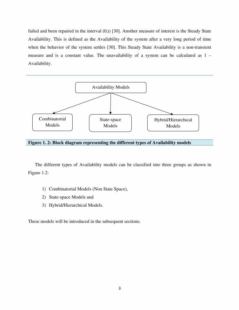
failed and been repaired in the interval (0,t) [30]. Another measure of interest is the Steady State
Availability. This is defined as the Availability of the system after a very long period of time
when the behavior of the system settles [30]. This Steady State Availability is a non-transient
measure and is a constant value. The unavailability of a system can be calculated as 1 –
Availability.
The different types of Availability models can be classified into three groups as shown in
Figure 1.2:
1) Combinatorial Models (Non State Space),
2) State-space Models and
3) Hybrid/Hierarchical Models.
These models will be introduced in the subsequent sections.
Figure 1. 2: Block diagram representing the different types of Availability models
Availability Models
Combinatorial
Models
State-space
Models
Hybrid/Hierarchical
Models
4
Section 1.2.1 COMBINATORIAL MODELS
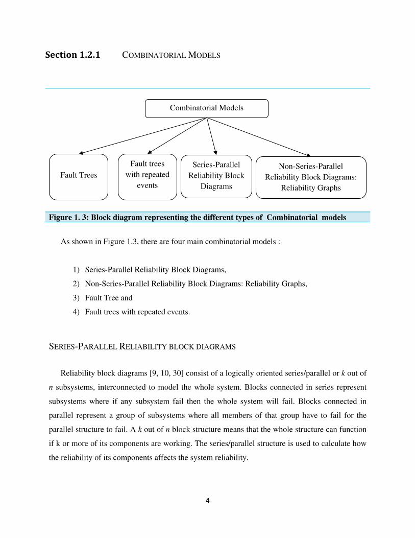
As shown in Figure 1.3, there are four main combinatorial models :
1) Series-Parallel Reliability Block Diagrams,
2) Non-Series-Parallel Reliability Block Diagrams: Reliability Graphs,
3) Fault Tree and
4) Fault trees with repeated events.
SERIES-PARALLEL RELIABILITY BLOCK DIAGRAMS
Reliability block diagrams [9, 10, 30] consist of a logically oriented series/parallel or k out of
n subsystems, interconnected to model the whole system. Blocks connected in series represent
subsystems where if any subsystem fail then the whole system will fail. Blocks connected in
parallel represent a group of subsystems where all members of that group have to fail for the
parallel structure to fail. A k out of n block structure means that the whole structure can function
if k or more of its components are working. The series/parallel structure is used to calculate how
the reliability of its components affects the system reliability.
Figure 1. 3: Block diagram representing the different types of Combinatorial models
Combinatorial Models
Fault trees
with repeated
events
Series-Parallel
Reliability Block
Diagrams
Non-Series-Parallel
Reliability Block Diagrams:
Reliability Graphs
Fault Trees

5
In a block diagram model, each component can have a failure rate, a failure probability, a
failure distribution function or the unavailability associated with it. Each subsystem is assumed
to operate independently of each other.
RELIABILITY GRAPHS
Reliability Graphs [30] are constructed using a set of nodes and edges. The edges represent
subsystems that can fail and are interconnected by nodes to model the entire system. There are
two unique nodes called a source and a sink. A source has only outgoing edges to other
subsystems. A sink has only incoming edges from other subsystems. A system modeled by a
Reliability Graph conceptually fails if there is no path from source to sink. Like Reliability Block
diagrams, the edges can be assigned a failure rate, a failure probability, a failure distribution
function or the unavailability associated with it. Again each subsystem is assumed to operate
independently of each other.
FAULT TREES
Fault trees [9, 10, 30] use a logical tree like structure to model system failure and captures all
the individual component events that can cause a system to fail. The Fault Tree represents,
pictorially the combination of events that can cause the system to fail. A failure event at the top
level of the Fault Tree is reduced to events at lower levels by means of logic gates. Each lower
level event can be further reduced until basic events are reached which require no further
reduction.
Each logic gate has inputs and outputs. Logic gates are connected so that the inputs can be
either a basic event or the output of another gate. An OR gate, for example, will output a logic
‘1’ if and only if one or more of its inputs are logic ‘1’. A AND gate will output a logic ‘1’ if and
only if all of its inputs are logic ‘1’. A k out of n gate will output a logic ‘1’ if k or more of its
inputs are ‘1’. For each Fault Tree the top most gate will have a single output called the top level
event which represents a system failure. The basic Fault Tree assumes also assumes that each

6
system operates independently of each other. A more detailed description of Fault Trees is given
in Chapter 3.
NON INDEPENDENCE
The combinatorial models described above assume that subsystems operate independently of
each other. There are cases in which subsystems are repeated in the overall model and are not
independent. For example, consider a system with two CPUs sharing the same memory module.
This shared memory would be considered as a repeated event. A repeated event cannot be
modeled as two independent systems. Some methods for solving Reliability Graphs and Fault
Trees with repeated events are [30]:
• Factoring or conditioning and
• SDP (sum of disjoint products)
Section 1.2.2 STATE-SPACE MODELS
In order to model complicated interactions, sequences and dependencies among systems or
components, more complicated state space models can be used. Two dominant examples of these
Figure 1. 4: Block diagram representing the three types of homogeneous Markov models
Markovian Models
Continuous-time
Markov chains
Markov reward
models
Discrete-time
Markov chains

7
models are Markov Chains and Stochastic Petri-nets [30, 33]. Stochastic Petri nets can be used
for easier specification, generation and solution of an underlying Markov model. In Figure 1.4,
homogeneous Markov models are divided into three groups, Discrete, Continuous and reward
models. Non-Markovian models include the Semi-Markov and Markov regenerative processes as
shown in Figure 1.5.
MARKOV CHAINS
Generally, a homogeneous Markov Chain consists of a number of states that the systems can
exist in and arcs that allow the system to transition from one state to the next. Understanding the
behavior of a system requires evaluating the states in the Markov Chain. Since the Markov
Chains attempt to represent all the relevant states in the system, a state space explosion can
occur. This can result in a huge model which is computationally expensive and difficult to
interpret. For example, a model with N components may require 2N states. The transitions in a
Markov Chain can be defined by probabilities or rates for discrete and continuous systems
respectively. A key requirement of homogeneous continuous time Markov Chains is that the
sojourn time (the time spent in a state) must be exponentially distributed.
Markov Chains that use reward models associate a reward function with each state. The
reward obtained per unit time spent in a particular state can be calculated. The reward associated
with a state denotes the performance level given by the system while in that state.
Non-Markovian model is the Semi-Markov process. Recall that a continuous time
homogeneous Markov chain requires the sojourn time to be exponentially distributed. For a semi
Markov process, this restriction no longer exists and the sojourn time can be any distribution
function. A more detailed description of Discrete and Continuous Time Markov Chains is given
in Chapter 3.

8
PETRI-NETS
A Petri-net is constructed with places, transitions, and arcs. Places may contain tokens and
transitions determine how many tokens or when tokens are transferred from one place to the
next. As an example a place can represent a particular state of the system and transferring tokens
to other places represents how active that is. For example, in a traffic light system, each color
light can be represented by a place. To indicate that a light is on, a token can enter that
previously empty place. When the token leaves, that place is empty again, meaning that the light
is off. For Stochastic Petri Nets, the transitions can be timed events, given by rates. These rates
are associated with each transition and determine the rate at which tokens are moved are from
one place to another. Stochastic Petri Nets can be converted back to Markov Chains. Petri-nets
can also result in a state space explosion problem.
Section 1.2.3 HYBRID/HIERARCHICAL MODELS
Hybrid/Hierarchical Models [30] combines two or more models. Inputs are obtained from
one and fed into the other until a top level system is defined. Combinatorial models, such as
Fault Trees are not good at modeling sequencing events. Nevertheless, they are very good at
modeling parts of the system that are not sequenced, furthermore they do not suffer from a state
space explosion problem. An example of a Hybrid/Hierarchical model is Fault Tree – Markov
model. The Fault Tree is used to model the top level description of the system and Markov
Chains are used to capture any sequence dependent and interacting components. Availability
measures are calculated from the Markov Chains and used as inputs to the Fault Trees to
calculate the overall Availability of the system.
In this research Fault Trees have been used to provide a top level model of the system while
Markov Chains are used to model the subsystems that require sequencing and/or interaction with
each other. In doing so the state explosion problem is significantly reduced, the top level
description is easily understood from the Fault Tree logic and calculating the availability is less
computationally intensive than a full state space model.
9
Section 1.3 MOTIVATION
This work was motivated by the lack of a modeling method that has been applied to virtual
systems and cloud computing in a way that incorporates hardware, software and response time
failures. One very important aspect of this research is that it examines and integrates the effects
of response time failures. Response time failures occur when a job issued to the system does not
complete on time and the system is viewed by the user as failed. A simple example is a user
waiting for a web page to load and receives a time out response. The user may assume that the
web server has failed when in fact the software and hardware systems of the web server are still
fully functional. In this case the server’s performance may be inadequate in servicing all its
requests at that time resulting in a time out response. A traditional hardware and software
availability model would still report that the system had not failed and is still highly available
because it did not consider response time failures. A detailed description of the previous research
is given in Chapter 2 and a brief description will be given here. Previous works have considered:
1) A single availability model for the hardware system,
2) A single availability model for the software system,
3) A unified availability model for hardware & software Failures in virtual systems,
4) A single availability model for response time without hardware or software Failures,
5) A single availability model for hardware & software Failures, merged with response
time failures that only occur due to limited buffer size. In this case response time
failures that are due to virtual processing and failed resources were not considered.
In cloud computing, buffer sizes are very large and response time failures very rarely occur
due to inadequate buffer sizes. Response time failures will generally occur when there isn’t
adequate processing power. This is particularly important when processing power is shared by
many different virtual systems, applications and users. In virtual systems, processing power at
the hardware level is shared among the virtual CPUs. In modeling virtual systems, variables such
as the Virtual CPU speed, the number of Virtual CPUs and the number of Virtual Machines,
must also be taken into consideration. This has not been done in the previous works on virtual or
cloud systems.

10
Additionally, cloud systems often communicate with each other in order to complete a task.
For example a web server may need to access a database server in a different cluster. Present
models of virtual systems do not include this type of communication and how they affect
response time failures.
Cloud systems are designed to be highly available. This is because they are designed with
multiple redundancies or replicas providing the same services. This can also increase throughput,
directly affecting response times. Even though some replicas will fail, traditionally the system is
considered to be still highly available because other replicas are still up and providing the
required service. In reality failed replicas can reduce performance if they were being used to
increase parallel processing. Such a system will have jobs taking longer to complete, directly
affecting the response time of the system. It is therefore important to model failed replicas and
their effect on the response time. From a user point of view if a job or request does not complete
on time the system is considered to have failed. This requirement has not been incorporated into
availability models for virtual and cloud systems.
Section 1.4 CONTRIBUTIONS
The models and measures used in this research already exist. The novelty of the contributions
is based on combining these models and measures to calculate the availability in a way that has
not been done for virtual systems. The main contributions are as follows:
An integrated model was developed for virtual systems that combine hardware, software and
response time failures, encapsulating the following features:
• Include layered communication between computing systems in the model:
− Layered communication multiple servers that need to communicate with each
other in order to fulfil a given request. For example, a user request sent to a web-

11
server, may require that web-server to communicate with a database server in
order to obtain data to fulfil the user request.
• Incorporate relevant virtual machine variables that directly affect response failures:
− Number of Virtual machines & CPUs, Virtual CPU speed.
• Unique Response Time models that correspond to each unique hardware/software
configuration.
− A system can experience failures at any time. When modules in the system fail, the
hardware or software configuration changes. For example, consider a system
with two databases. Two databases that are fully functional would be one
configuration. If one database fails then the new configuration would only have
one database. Two databases would be able to service more requests than a
single one.
Each configuration directly affects the performance of the system. The
performance is in turn determined by its response time model. Each response time
model corresponds to a hardware and software configuration. It is therefore
important to design the modeling system to combine each response time model
with its unique hardware and software configuration.
The research in this thesis started with the article written by Paharsingh et. al. [24]. In [24] a
model for the triple modular redundancy (TMR) system that exploits virtualization was
developed. This TMR system, reduced the number of actual hardware systems from three to two.
With only two hardware units, the availability was approximately the same as a traditional TMR
system with three hardware units. The models used in [24] for the virtual system combined Fault
Trees and Markov Chains. These modeling techniques were later modified to combine the
hardware and software models with response time models and presented by Paharsingh [25]. The
inclusion of the response time models was necessitated by the need to extend the analysis to
larger virtual system such as clouds.

12
Section 1.5 THESIS ORGANIZATION
This thesis will is organized as follows: A review of virtual system and cloud computing is
given in Chapter 2. Chapter 2 examines relevant research that has been done in assessing the
availability of virtual and cloud computing systems. The models used in this research are
explained in details in Chapter 3. These models are Markov Chains, Fault Trees and Queuing
Networks [30]. Chapter 4 demonstrates the modeling technique on a small cluster and provide a
discussion of results. In Chapter 5 the conclusion and future work are discussed.
13
CHAPTER 2
BACKGROUND: VIRTUAL SYSTEMS AND RELATED RESEARCH
Section 2.1 INTRODUCTION
An introduction to Virtual Systems, including Cloud Computing and the modeling techniques
developed in assessing availability is discussed in this chapter. In Section 2.2 Virtualization and
the relevant technologies in Virtualization are explained. Cloud Computing and the different
layers in the cloud stack model are presented in Section 2.3. In Section 2.4 hardware, software
and response time failures are discussed as they relate to virtual systems such as clouds. The
most relevant research in this field is examined in Section 2.5 followed by conclusion in Section
2.6.
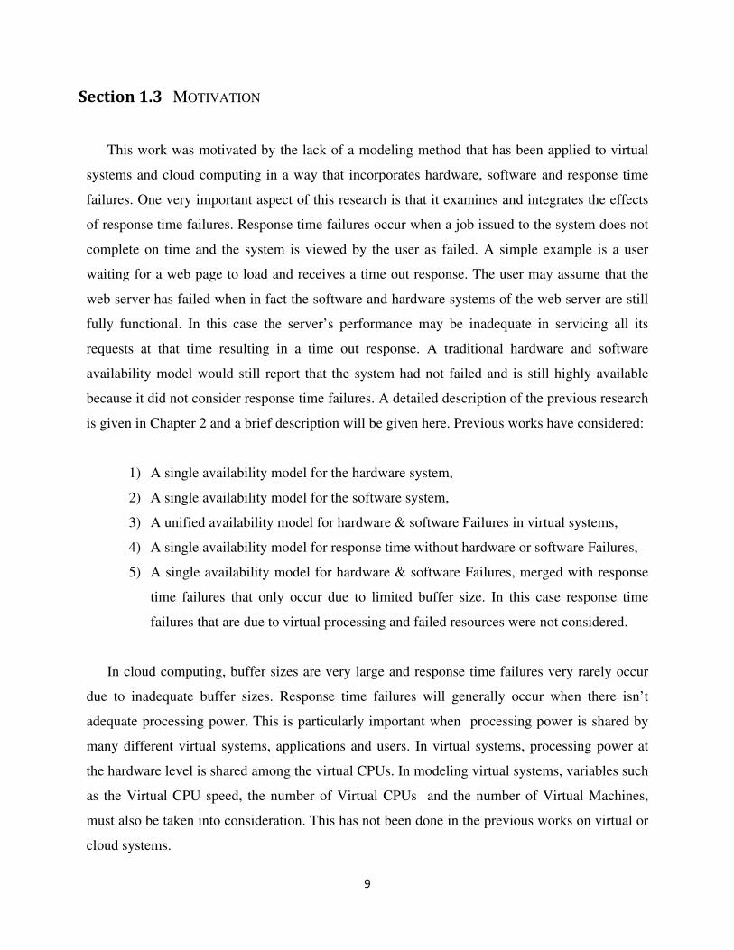
Figure 2. 1: A bare-metal virtualization system common in cloud computing environments

14
Section 2.2 VIRTUALIZATION
Virtualization of a computer hardware system is the software implementation of that system,
mapped to real hardware. The software implementation includes Processors, Memory, I/O
Devices and Bios that are mapped to a real hardware system [7]. This software implementation
of the hardware system is usually referred as the Virtual Machine. Two main categories of
Virtualization are: Full Virtualization and Para-Virtualization [39].
FULL VIRTUALIZATION
With full Virtualization, the guest OS is not aware of that it is running on virtual hardware.
The guest OS can be migrated to another virtual machine or native hardware without any
modification to the OS. This results in fast migration. The Virtual machine is completely isolated
from the underlying hardware. The three main methods of full Virtualization are: Bare Metal, OS
Hosted and Kernel Embedded.
In Bare-metal systems, the Virtualization layer runs directly on the host's hardware and
independently of a general purpose operating System. This Virtualization layer is called the
hyperadvisor or Virtual Machine Monitor (VMM). The VMM is responsible for managing the
Virtual Machines installed on it and for efficiently sharing hardware resources with those Virtual
Machines. As shown in Figure 2.1, the VMM encapsulates and manages the hardware system/s.
The Virtual Machine/s (VMs) is/are running on top of the VMM and the OS and Applications,
depicted as application services are running on the VMs. Each VM hosts a single OS. Examples
of Bare Metal systems are VMware ESXi [36] and Xen based systems [1].
In OS Hosted Virtualization the VMM operates on top of the Operating System rather than
directly on the hardware system. The system is shown in Figure 2.2. All the layers above the
VMM remain the same as in Bare Metal systems. Some examples of OS Hosted Virtualization
systems are VMware Server [37], Oracle’s VirtualBox [23], and VMware Workstation [38].

15
Figure 2. 2: An example of OS Hosted virtualization
Kernel Embedded Virtualization is similar to OS hosted Virtualization in that the VMM is
still hosted by the OS. The major difference is that the VMM is embedded in the OS kernel. The
main advantage of this system over OS hosted is that it offers improved performance. An
example of Kernel Embedded Virtualization is the Linux Kernel-based Virtual Machine also
known as KVM.
PARA-VIRTUALIZATION
In order to speed up the Virtualization process, the guest OS is made aware of the VMM. The
guest OS is modified so that it can communicate directly with the VMM. For a Full
Virtualization system, the guest OS has to communicate with the VM. The VM then has to
communicate with the VMM as shown in Figures 2.1 and 2.2. A Para-Virtualization (also
referred to as an OS Assisted Virtualization System) reduces the communication overhead by
allowing the guest OS to communicate directly with the VMM for some instructions. This
method reduces some overhead and allows a Para-virtualized system to execute with increased
speed. Xian based systems are examples of Para-Virtualization. The main disadvantage of Para-
16
Virtualization is that only a modified OS can be hosted. This presents problems during
migration.
Section 2.3 CLOUD COMPUTING
Buyya et al. [7] defined Cloud Computing as: “Cloud is a parallel and distributed computing
system consisting of a collection of interconnected and virtualised computers that are
dynamically provisioned and presented as one or more unified computing resources based on
service-level agreements (SLA) established through negotiation between the service provider and
consumers.” Vaquero et al. [7] described Cloud Computing as: “Clouds are a large pool of
easily usable and accessible virtualized resources (such as hardware, development platforms
and/or services). These resources can be dynamically reconfigured to adjust to a variable load
(scale), allowing also for an optimum resource utilization. This pool of resources is typically
exploited by a pay-per-use model in which guarantees are offered by the Infrastructure Provider
by means of customized Service Level Agreements.”
Essentially Cloud Computing represents a large computing resource, built on the
Virtualization of hardware systems. Virtual resources can be sold to customers as services. These
services [44] can be categorized as: Infrastructure as a Service (IaaS), Software as a Service
(SaaS) and Platform as a Service.
IaaS offers virtual hardware systems or virtual machines. A customer can purchase a virtual
hardware system in terms of CPU and Memory specifications. Amazon [3] offers this type of
cloud computing service. A virtual machine can be created and destroyed, turned on or off as
required and can host many different types of operating systems. In most cases the virtual
machines come preloaded with an OS of choice.
The Google App-engine [26] is an example of PaaS. The Google App-engine provides an
environment for the development scalable web applications without worrying about setting up
hardware resources as in the case of IaaS. The PaaS layer operates above the IaaS layer and
customers can develop applications and have them hosted at this layer.

17
The SaaS layer of the cloud stack occurs above the PaaS layer and offers software to
customers as a service. Rather than paying for licenses and installing software locally on a
personal computer, customers can access these applications online through web portals.
Microsoft [21] and Google [13] offers applications online for word processing and spreadsheets,
that can be accessed through a web browser.
Section 2.4 TYPES OF FAILURES
HARDWARE FAILURES
The cloud system is summarized in Figure 2.1. The hardware systems at the bottom of the
figure are managed by the VMM. This configuration represents a Bare Bone virtualized system
as explained in Section 2.2. A single hardware system can fail if any of its components fail such
as processor or power supply. In real systems, failures of these components are highly masked by
incorporating enough redundancy so that the probability of a failure is very low. For example a
typical server may have dual power supplies and multiple storage units configured using RAID.
Normally these redundant parts are hot swappable, i.e. if one fails it can be removed and
replaced without shutting down the system.
Even with redundancies, failures still occur. Since the cloud architecture is built on top of the
hardware systems, a hardware failure can take down the whole system. It is therefore essential to
model hardware failure in such a way that, the model allows the designer to increase and
decrease redundancy.

18
Figure 2. 3: An example system demonstrating Cloud Computing
SOFTWARE FAILURES
In Figure 2.3, the VMM, VMs and all application servers (OS and applications) are
considered to be software systems. A software failure can occur if any of these systems fail. A
failure at a lower level can induce failures at upper levels that are dependent. For example, if the
VMM on the left side of Figure 2.3 fails, all VMs and Application Services above it will also
fail.
RESPONSE TIME FAILURES
User perceived or response time failures occur when a user is expecting results at a certain
time and the system fails to meet that deadline. In Figure 2.3 requests are entering the system at
the top where the application servers attempt to fulfil these requests. In fulfilling these requests,
sub-requests are sent down to the VM, VMM and finally to the hardware system. Response time
failures can therefore be triggered by both software and hardware failure. In virtual systems such
as the cloud, these failures manifest at the IaaS [12, 35] and above layers. They can also be
triggered by inadequate processing power. When this happens due to inadequate processing

19
resources, it can be triggered by the user not purchasing enough VMs, the number of Virtual
CPUs or the cloud provider not allocating enough processing power to the VMs. The latter case
can also be due to too many VMs migrated to the same server. In modeling the availability of
these systems, it is absolutely necessary to combine hardware, software and response time
failure.
As mentioned in Chapter 1, in modeling response time failure, it is also important to consider
systems that require communicating with multiple servers in order to service a request. For
example, a web-server may need to access a database server. In Figure 2.3 this is represented by
requests entering the application servers on the left of the diagram, after partially servicing the
request, a database access is required from the application servers on the right of the figure.
When the database request is completed, the result is sent back to the servers on the left. On
entering the server on the left, additional processing takes place at which the request may be
fully completed and leave the system as a serviced request.
Section 2.5 RELATED RESEARCH
Models exist for the three failures of interest (software, hardware and response time). These
models include: Reliability Block Diagrams (RBDs), Fault Trees, Markov Chains, Petri-Nets,
Reliability Graphs, Layered Queuing Networks (LQN), Queuing Networks (QN) [6, 9, 10, 20,
30, 33] and a few others. LQNs and QNs are normally used for performance modeling with a
few authors demonstrating their applicability to response time failure. An integrated model that
encapsulates problems unique to the cloud and virtual systems that are dependent on shared
processing power did not exist during this research. This research combines both Markov Chains
(MCs) and Fault Trees (FTs) to model virtual systems. Many analysis methods exist for cloud
and virtual systems. Some examples are, cost analysis [11, 16, 17, 34, 42], software rejuvenation
models [18, 22, 29, 32] and models for hardware, software or response time failures. In later
cases, these can be further defined in terms of performance and availability analysis. In this
Section articles related to modeling availability in cloud computing will be presented.

20
In solving a particular problem, the modeling techniques presented in these articles may
incorporate any of the following: Virtual Machines, hardware, software or response time failures.
These articles represent significant work in specific areas for specific systems and provide
accurate solutions within the domain of the problem/s being analyzed. When shifted into the
domain of the research presented in this thesis, they provide some parts of the complete solution.
In that light they should not be interpreted and are not presented as inadequate work. Since this
research requires an analysis of Virtual Systems and response time failures, the articles are
organized as follows: Models without response time failures or Virtual Systems, Models for
Virtual Systems with no response time failures and Models for response time failures without
Virtual Systems.
MODEL WITHOUT RESPONSE TIME FAILURES OR VIRTUAL SYSTEMS
An approach to modeling complex behavior is to use a hybrid system, consisting of two or
more classes of models, such as combinatorial and state space. Smith et. al. [31] developed
accurate availability models for IBMs blade server systems to evaluate the availability of
different hardware architectures. The models developed, targeted hardware and software
systems. In order to avoid computationally intensive models that are fully state based, the authors
used a practical two level hierarchical approach. This approach integrated, combinatorial models
and state space models. Each subsystem in the servers is modeled using Markov Chains while
the entire system is modeled as a Static Fault Tree. The Markov Chains provide the inputs to the
Static Fault Trees, thereby reducing the size of the model as compared to a fully state based
system.
While the Static Fault Trees can easily represent the logical availability structure for the
entire system, they are not natively efficient at modeling dynamic behavior. Dynamic Fault Trees
can model the dynamic behavior but they are usually converted to Markov Chains in order to
solve them. The authors have therefore used Markov Chains rather than Dynamic Fault Trees.
21
MODELS FOR VIRTUAL SYSTEMS WITH NO RESPONSE TIME FAILURES
Kim et.al. [15] modeled a server based hardware and software system that supports
virtualization. The Markov-Fault-Tree system that was used is similar in concept to the method
used by Smith et. al. [31]. The Fault Trees were used to model the top level behavior of the
system. They used Markov Chains along with a fine grain approach that models every significant
component of the hardware systems such as Power Supply, Ethernet, CPU, etc. The Markov
Chains essentially modeled hardware dependencies along with failures and repairs. The failures
and repairs of virtual machines and software subsystems were also modeled as Markov Chains.
The Markov Chains were solved and used as inputs to the Fault Trees.
Paharsingh et. al. [24] developed a triple modular redundancy (TMR) system that exploits
virtualization, reducing the number of hardware systems from three to two. With only two
hardware units, the availability was approximately the same as a traditional TMR system with
three hardware units. Additionally, the proposed system is more immune to software failures
than the traditional TRM system. The model combined Fault Trees and Markov Chains using
similar techniques as Smith et. al. [31].
Wei et. al. [41] proposed a model for the analysis of virtual clusters. Their model is
essentially a hybrid method which combines both combinatorial and state space models. The
combinatorial model is a RBD model which models the system as a whole. The state space
model is a Markov Chain which models the internal blocks of the RBD model. Essentially, the
RBD model is designed so that, individual clusters with ‘m’ servers (per cluster) are connected in
series. For each cluster, the ‘m’ servers are connected in parallel. The Markov Chains are used
to model the combined availability of the VM, VMM and the hardware system within each
server.
Che et. al. [8] designed an availability model for modeling Cluster Nodes built on virtual
machines. The models are built entirely from Markov Chains and focuses mainly on the different
states that the virtual machine can exist in. According to Che et. al. [8], a virtual cluster node can
be in five states: Normal, Unsteady, Rejuvenation, Switchover and failure.

22
• In Normal mode, the virtual cluster node is fully functional.
• When in an Unsteady state, the virtual cluster node is still available but operates
with a decreased performance.
• In order to operate efficiently, the virtual cluster node needs to move back from
Unsteady to Normal mode as soon as possible. During this transition, the system
is considered to be in a Rejuvenation state.
• If the node is in an Unsteady state and faults are unrecoverable, then a Switchover
occurs changing the system to a standby node.
• If the virtual cluster node completely stops working then it ends in a failure state.
The reliability of virtual systems running on specific servers was modeled by Ramasamy et.
al. [28]. The modeling technique used was entirely combinatorial, expressed as an RBD diagram.
For example, the hardware system, VMM and each set of VMs are all connected in series. The
set of VMs providing the same service is connected in parallel. All systems are assumed to
operate independently of each other.
MODELS FOR RESPONSE TIME FAILURES WITHOUT VIRTUAL SYSTEMS
Kaniche et. al [14] in principle, uses similar concepts to Smith et. al. [31], for modeling
hardware and software failures. Additionally, the authors outlined a system for combining
availability measures from various models. The mathematical equations that they had used to
combine the outputs of the models could also have been derived from Reliability Block
Diagrams (RBDs) or Fault-Trees without repeated events. Repeated events are used to represent
components that influence multiple sections of the overall system. Their research incorporated
response time failures that are due to inadequate buffer sizes. The response time of a server was
estimated using a M/M/1/K Queue (please see Kendall’s notation, Chapter 3) which has one
server and a buffer size of K. The probability of an arriving request getting lost is computed
using derived formulas which take the buffer size into account. The authors answer the important
question, as to how a limited buffer size will affect response time failures.

23
The focus of Mainkar's research [19] was on response time failures that are due to server
processing power. Availability is modeled as the probability that at any time a required minimum
fraction of the transactions is finished within a given deadline. This definition is dependent on
server processing times and request arrival rates. It assumes that server buffer sizes are large
enough to accommodate the incoming requests. The author presented two methods for modeling
the system. The first method was Stochastic Reward Net, and resulted in a very large model as
expected. The second technique used an approximation method and modeled the server as an
M/M/c Queue. The M/M/c Queue was solved by deriving an approximation formula based on
the Hypo-exponential and Erlang distributions.
Wang et. al. [40] developed a modeling system that consisted of Markov Chains, User
Interaction Graphs and Stochastic Reward Nets. The authors had focussed their research on
finding the user perceived availability. This availability was calculated based on whether or not
the system is functioning and services the user request at the time when the user makes that
request. It doesn’t matter if the system had failed when the user isn’t making a request. Wang et.
al. [40] describes user perceived availability as, “During a user interaction (session) with the
system, the user issues multiple requests at different time points for different system resources.
The unavailability of requested resource will cause the request to fail. The service availability is
the probability that all requests are successfully satisfied during the user session”.
An estimation method was presented for calculating the response time distribution for server
based system without hardware or software failures, by Zheng et.al. [43]. Their web server
example was modeled using LQNS. The mean response time and variance were obtained from
the simulator and plugged into the gamma distribution equation. The authors demonstrated that
the estimation is accurate particularly for probabilities > 0.9.
Section 2.6 CONCLUSION
Evaluating the availability in Virtual and Cloud systems can be very useful in understanding
how various system configurations will affect the downtime. This data can be used to design
24
more robust and cost effective systems. In virtual systems where users are allowed to purchase
virtual machines and build their system of servers, modeling the correct virtual machine
variables can be very important. These variables include the number of virtual CPUs per server,
the speed of each virtual CPU and the number of virtual machines. Another important
characteristic in cloud systems is the necessity for servers to communicate with other servers.
Including this into the availability would be very useful since if one or more servers fail to
communicate, requests are not likely to be serviced.
Combining hardware and software failures with response time failures are imperative since
users will perceive poor response times as failures. Models for virtual and cloud systems can
easily become huge and computationally expensive. The likelihood of this happening
significantly increases if the models are entirely state based. An analysis of the relevant articles
on virtual systems reveal that the modeling techniques usually involve a hybrid modeling system
such as combining combinatorial with state based. In fact this is often true when modeling large
systems on a whole. Additionally the relevant research articles on response time failures have
demonstrated the significance of incorporating queuing networks.
In order to reduce the size of the model and avoid the state space explosion problem a hybrid
modeling technique will be used to develop the modeling system for this research. The hybrid
model uses Markov Chains and Fault Trees to model hardware and software failures. Response
time failures are modeled using Queuing Networks. Although these Queuing Networks are
solved by converting them to Markov Chains, a method of reducing the size of the Chains will be
used. This method is based on work done by Trivedi [33] for M/M/ , M/M/1 and M/M/c
Queues. For M/M/c queues it is similar in principle to the method used in Mainkar's research
[19].
Also unique to this research is the modeling of different hardware and software
configurations. The configuration of every computing system changes when a subsystem fails.
These changes occur simply because the system has less functional components and can operate
with decreased performance or none at all. Decreased performance can result in a decrease in

25
response times. In Chapter 3 the theory and research done in developing Markov Chains, Fault
Trees and Queuing Networks will be presented.

26
Section 3.1 INTRODUCTION
The techniques used in this research to model virtual systems are discussed in this chapter.
The models used are Markov Chains, Fault Trees and Queuing Networks. These models are
combined with chapter 4 to enable the analysis of virtual and cloud systems for availability. Fault
Trees are used to specify the top level architecture of the virtual system and Markov Chains are
used as inputs to the Fault Trees. The Markov Chains model dynamic dependencies that cannot
be captured by Fault Trees. The Queuing Network model will be used to find the response time
CHAPTER 3
BACKGROUND: MODELS AND RELATED RESEARCH
Figure 3. 1: A Discrete time Markov Chain, representing a server that
is functioning in state A and has failed in state B
A B

27
probability for requests completing by a certain time. The discussion will start by introducing
both discrete and continuous time Markov Chains. Solving continuous time Markov Chains are
necessary for computing steady state and transient availability. These two availability measures
are of relevance to this research and will be demonstrated in section 3.2. Fault Trees will be
examined in section 3.3, demonstrating how probabilities can be calculated. In section 3.4
Queuing Networks are introduced as they relate to this research. An efficient and simplified
method is presented that allows the calculations of transient response times for the Queuing
Networks. In Section 3.5 a review and conclusion of this chapter are presented.
Section 3.2 MARKOV CHAINS
Markov Chains were invented in 1906 by a Russian mathematician named Andrei Markov
and has since been extensively used in engineering. A Markov Chain can be thought of as a state
diagram with some mathematical restrictions. The representation of a system is modelled by
defining all the relevant states that the system can be in. These states are connected by arcs. Each
arc is used to represent a transition from one state to the next. The arc can be the probability of
moving into the next state or the rate at which the system will move into the next state.
DEFINITIONS [30]
1. Define a random variable as a function that maps each element of a sample space
to a real number. The usual symbol for a random variable is X. For example, assume an
experiment is carried out with a single coin which is flicked twice each time. There are four
possibilities: HH, HT, TH, and TT. Let X represent the number of heads from each trial.
There can be 0, 1, or 2 heads.
28
The probabilities associated with each possible value of X is given in table 3.1. The
probability of getting 0 heads is 0.25; 1 head, 0.50; and 2 heads, 0.25. Table 3.1 is an
example of a probability distribution for a discrete random variable.
Table 3. 1 The probability for the number of Head from
tossing a coin twice
Number of heads, x Probability, P(x)
0 0.25
1 0.50
2 0.25
A probability distribution, can be used to understand the behavior of a system. For
example, the probability of getting 1 head is P(X = 1). This is read as the probability that
the random variable X = 1. Hence, P(X = 1) = 0.50.
2. Define a stochastic process as a family of random variables X(t) on a sample
space.
3. Define states as the values assumed by X(t)
4. Let the set of all states be defined as the state space
If X(t) is a discrete stochastic process, the let Pr(X(tn) = j) be interpreted as the probability
that the process is in state j at the time tn. X(t) is a Markov Chain provided that, for times t1 < t2 <
....tn, the conditional probability of being in any state j is:
Pr{ X(tn) = j | X(tn-1) = in-1, X(tn-2) = in-2, ....... , X(t0) = i0} = Pr{ X(tn) = j | X(tn-1) = in-1} (3.1)

29
The above equation implies that a Markov Chain after a transition may depend on the state
immediately before and not on any states before that [30].
DISCRETE TIME MARKOV CHAINS [30]
1. Define as a matrix containing the probabilities of being in each state of the system
at discrete instant ‘n’.
2. Define ‘P’ as the system probability matrix which contains the probability of
transitioning from one state to the next. An important property of the P matrix is that it
rows must sum to 1.
For a homogenous Discrete Time Markov Chains, equation 3.2 gives the transient probability
matrix, . The matrix is calculated, given the previous probability matrix
and the system probability matrix of the Markov Chain P. Equation 3.2 will be
demonstrated later.
(3.2)
If the initial probability of being in each state is known, equation 3.3 can be used to
calculate the transient probabilities of the system.
(3.3)
STEADY STATE PROBABILITY [30]
If , the probabilities approach a steady state. Solving for in equation 3.4 gives
the steady state probability matrix for the system of states.

30
(3.4)
DISCRETE MARKOV CHAIN EXAMPLE
This example [30] will demonstrate how to apply equation 3.3 & 3.4. Figure 3.1 represents a
Markov Chain for a system with one CPU. In State ‘A’ the System has one CPU working and is
functional. In state ‘B’ the system has no CPU working and has failed. Moving from state ‘B’ to
‘A’ represents a repair function while ‘A’ to ‘B’ represents a failure.
Each transition is represented by the probability of moving from one state to the next or
remaining in the same state. For example, the probability of moving from state A to state B is
0.7. The Markov Chain has to be converted to a probability matrix (P) in order to carry out
mathematical operations on it. Equation 3.5 gives the probability matrix for the system.
, Probability matrix = P. (3.5)
To demonstrate how equation 3.3 works, let’s assume that . This means that
the initial probability that the system is in state A is 0.8 and the probability that the system is in
State B is 0.2.
=> =
=
This means that the probability that the system is UP in state ‘A’ after the first discrete instant
0.26, likewise the probability of the system being down is 0.74.

31
Steady State Calculations
From equation 3.4 we have,
=> 0.3 +
0.7 +
Also, => + = 1
Solving gives
= [0.125 0.875]
This means that the probability that the system is UP in state ‘A’ after a very long time is 0.125,
this is also the long term or steady state availability of the system.
CONTINUOUS TIME MARKOV CHAINS [30]
A homogeneous continuous time Markov Chain must also satisfy equation 3.1 and transitions
from one state to the next are rates rather than probabilities. There are many measures that can be
obtained evaluating these Markov Chains. This discussion will focus on the relevant techniques
and measures used in this research. The measures of interest include calculating the transient and
32
steady state availabilities for the Chain. Markov Chains with absorbing states are particularly
important when solving Queuing Networks. In this case finding the transient probability of being
in an absorbing state will be important, Queuing Networks will be discussed in section 3.4. The
formulas for evaluating these Markov Chains and the evaluation methods will be demonstrated
using examples.
If Q is the rate matrix then similar to discrete time Markov Chains,
(3.6)
Equation 3.6 is very similar to equation 3.2. An important property of this Q matrix is that the
rows must sum to 0. The steady state equations are given by the following:
(3.7)
(3.8)
CONTINUOUS TIME MARKOV CHAIN EXAMPLE 1
This example [30] will demonstrate how to find the transient equations and steady state
availability for a basic continuous time Markov Chain. Figure 3.2 is the Markov Chain for a
basic server system with two states A and B. Similar to the previous example when the server is
in state A the server is considered to be fully functional. When in state B, the server has failed.
The server transitions from state A to B at a failure rate of . If the server is in state B it can be
repaired at a rate of after which it will re-enter state A.

33
Figure 3. 2: A Continuous time Markov Chain, representing a server that is functioning
in state A and has failed in state B. The server fails at a rate of and is repaired at a
rate of
The rate matrix, Q is derived in a similar way as the discrete time Markov Chain. In this case
the rows must sum to zero. For this reason, is present in the matrix for AA. Likewise is
present for BB in the matrix.
With reference to equation 3.6, let
Now from equation 3.6 ,
[ ] =
,
A B
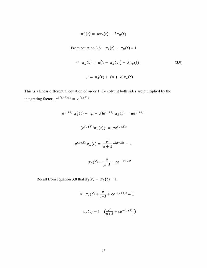
34
From equation 3.8 = 1
� (3.9)
This is a linear differential equation of order 1. To solve it both sides are multiplied by the
integrating factor:
=
Recall from equation 3.8 that = 1.
�
1 –

35
Since the system will be in state A at time 0, the probability of being in state A at t = 0 is:
�
c = 1 - =
� =
To compute the steady state probability of being in state 1, is evaluated as t goes to
infinity.
=
The of being in state B = , can be found in a similar way.
Note that the steady state probability could have also been calculated by using equations 3.7
and 3.8. Equation 3.7 has already been applied to generate equation 3.9. The next step is to apply
equation 3.8 by setting equation 3.9 equal to 0.
�
�

36
CONTINUOUS TIME MARKOV CHAIN EXAMPLE 2
In the previous example, it was demonstrated how to obtain the transient equation for a
particular state in a two state Markov Chain. This example demonstrates [33] how to find the
transient equation for a Markov Chain with an absorbing state. In this example the analysis in
principle is the same, in that the differential equations are obtained for each state. The
differential equation representing the state being analyzed is then solved for the transient
equation. This technique can be applied to other Markov Chains with each chain producing
different equations.
Figure 3.3 demonstrates a Markov Chain with an absorbing state C. The system represents a
two component redundant system. In state A both components are UP and can fail at a rate of 2
taking it to state B with only component UP. From state B, the failed component can be repaired
by the running component at a rate of which would take the system back to state A. Also
from state B the only one functioning component can also fail at a rate of taking the
system to the absorbing state C where the system remains because there are no
functioning components to repair it.
Figure 3. 3: A Continuous time Markov Chain with absorbing state C. The Markov
Chain represents a two component redundant system. In state A, both components are
UP, in State B one component is UP and in state C all components have failed.
A B
C

37
The technique follows the same principle as in the earlier example with the exception that in
this case only transient probabilities are important. The steady state probability of being in the
absorbing state will be 1 when ‘t’ approaches infinity.
The rate matrix is given by:
With reference to equation 3.6, let
=
To find the probability of being in state C at time ‘t’, a solution for is necessary. Taking
the Laplace transform of the differential equations will give the following:
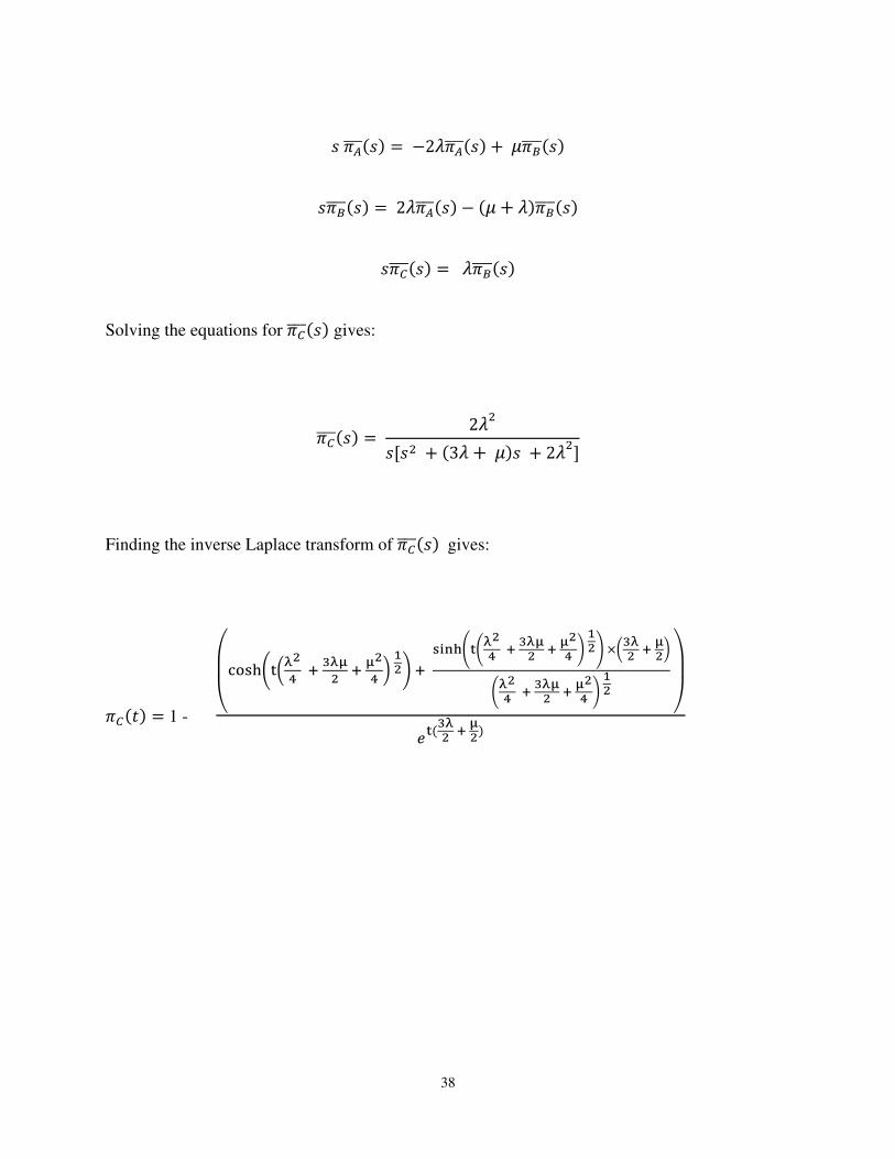
38
Solving the equations for gives:
Finding the inverse Laplace transform of gives:
1 -
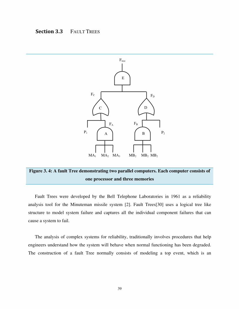
39
Section 3.3 FAULT TREES
Figure 3. 4: A fault Tree demonstrating two parallel computers. Each computer consists of
one processor and three memories
Fault Trees were developed by the Bell Telephone Laboratories in 1961 as a reliability
analysis tool for the Minuteman missile system [2]. Fault Trees[30] uses a logical tree like
structure to model system failure and captures all the individual component failures that can
cause a system to fail.
The analysis of complex systems for reliability, traditionally involves procedures that help
engineers understand how the system will behave when normal functioning has been degraded.
The construction of a fault Tree normally consists of modeling a top event, which is an
Ftree
E
C D
FA FB
FC FD
P1 P2
MA1 MA2 MA3 MB2 MB2 MB2
A B

40
identification of a system failure. This top level event is connected to one or more internal
system events through a system of gates, such as AND, OR and k-out-of-n. Although not in the
original specification, some FT tools will allow the inclusion of the NOT gate and related (e.g.
XOR) gates. Internal system events are basically failures of individual components or the effects
of external factors on the system or a combination.
The top event representing a failure is logically interpreted as the output of a single logic
gate. A logic level ”0” is used for operating and “1” for failure. A two input OR gate, for
example, can represent a system with two components connected to its inputs. A failure occurs if
both inputs fail or either inputs fail. A AND gate can represent parallel components for example,
components that have backups. A two input AND gate will represent a failure if and only if both
components at its input fail. A k out of n gate will indicate a failure if k or more of its inputs fail.
The design of the Fault Tree is done in two parts: Logical analysis, and a Probabilistic
analysis. The logical analysis is done by reducing the logical expression represented by the fault
Tree into minimal sets of logic expressions. This minimal set is the smallest possible
combination of failures required to cause a full system failure. The minimization can be done
with Karnaugh maps or Boolean algebra. The Probabilistic analysis is done by calculating the
probability of failure given the probability of each of the basic events occurring.
Traditional Fault Trees lack the accuracy required to model dynamic failure behavior in
particular those with a fault recovery process. One possible way to solve this problem is to divide
the system into several dynamic or static modules. The dynamic modules can be solved with
Markov Chains.

41
k-out-of-n gate,
Identically distributed inputs
k-out-of-n gate,
Non-identically distributed
inputs
(3.10)
Equation 3.10 [30] gives the expression for calculating the probability of failure, for each
gate [30]. In the case of AND, OR & k-out-of-n gate (Identically distributed inputs) ‘i’ indexes
the inputs for each gate. For the k-out-of-n gate (Non-identically distributed inputs) ‘j’ also
indexes the input of this gate. To find the overall failure equation, for a system with
many gates, , are computed for each gate and used as inputs for the
other gates that they are connected to. If the tree contains repeated events, then it can be solved
by factoring or by finding the Sum of Disjoint Products (SDP). For example, consider a system
with two CPUs sharing the same memory module. This shared memory would be considered as a
repeated event.
If factoring is used, the Fault Tree is divided into two separate Trees. One where the shared
memory module has failed and the other where the shared module has not failed. To compute the
overall distribution function, for the system, multiply the result for each case by the
probability that the case will happen, then add the products. If SDP is used, the Boolean equation
that describes the system failure is first derived. This equation is then made disjoint and equation
3.10 is applied to the new Fault Tree equation.
An Example of a FT is given in fig. 3.4. It represents a system with two computers running in
parallel. The first system consists of a single processor P1 with three memories MA1, MA2 and

42
MA3. Similarly, the second computer consists of a single processor P2 with three memories MB1,
MB2 and MB3. For each system, all the memories must fail for the computer to fail, hence the
memories are represented by a AND configuration. The processor or the all of its memories must
fail for a computer to fail, hence the processor and its memories are represented by an OR
configuration. The entire system is considered to fail if both of the computers fail, which is why
the top level AND gate is considered to fail if both of the computers connected to it fail.
Assuming that the failure rate of each memory and processor are exponential, then equation
3.11 gives the probability of failure at time t given the failure rate λ for each individual
component. To find equation 3.11 is fed into the leaves of the Tree for P1, MA1, MA2,
MA3, P2,MB1, MB2 and MB3 and the outputs, (See fig 3.4) for each gate is calculated
according to equation 3.10. This is then fed into the next respective gate and equation 3.10 re-
applied, until is obtained from the top most gate. Another approach is to find the
simplified Boolean equation for the tree and apply equation 3.10 accordingly to obtain .
F(t)0 = 1 – e-λt
(3.11)
For the Fault Tree in Figure 3.4, is calculated as follows:
AND Gate A: FM1(t) * FM2(t) * FM3(t) = FA
AND Gate B: FM1(t) * FM2(t) * FM3(t) = FB
OR Gate C: (1 – FP1(t)) * (1 - FA) = FC
OR Gate D: (1 – FP2(t)) * (1 - FB) = FD
43
AND Gate E: (FC) * ( FD) = Ftree
The fault Tree equation for the system:
Ftree = (FC) * ( FD)
Substituting for FC and FD gives:
= ((1 – FP1(t)) * (1 – (FM1(t) * FM2(t) * FM3(t)))) * ((1 – FP2(t)) * (1 – (FM1(t) * FM2(t) * FM3(t))))
To find the reliability of the system equation 3.11 is substituted for FP1(t), FP2(t), FM1(t), FM2(t)
and FM3(t), using the individual failure rate ‘λ’ for each component.
To find the Steady State unavailability of the system the steady state unavailability
substituted for FP1(t), FP2(t), FM1(t), FM2(t) and FM3(t). If P1, MA1, MA2, MA3, P2,MB1, MB2 and
MB3 are represented by Markov Chains, the steady state unavailability is found by summing the
steady state probabilities for all states where is system is down.
The steady state unavailability (SSU), now represents a single numerical probability rather
than an exponential function as in equation 3.11. This is because steady state values are constant.
In this research that numerical value is obtained from the Markov Chains representing the input
systems at the leaf level. F(t) is computed for each gate and equation 3.10 is then applied to
obtain a numerical value for . This final numerical value gives the system SSU. The
Steady State Availability = 1 – SSU.

44
Section 3.4 QUEUING NETWORKS
In 1909 Agner Krarup Erlang, published the first paper on Queuing theory. Queuing theory
has developed immensely since then and a lot of work has been done in computer science,
mathematics and engineering. A complete discussion is beyond the intention and extent of this
thesis, only the areas relevant to this research will be presented with a brief introduction to other
areas.
QUEUING STATION [33]
The basic unit of a Queuing Network is a Queuing station. A Queuing station is shown in
Figure 3.5. It consists of a buffer and a processor/server. The buffer can be infinite or finite and
the server segment can consist of one or more identical servers. Jobs can enter the buffer at a
rate indicated by in Figure 3.5 and are serviced by the server/processor at a rate of µ. Serviced
jobs will leave the system at a rate of . Which job is taken from the buffer and processed
depends on the Queuing discipline. Some common Queuing disciplines are [5]:
• FCFS (First-Come-First-Served): The jobs are served in the order of their arrival.
Figure 3. 5: A representation of a single Queue. Requests arrive at a rate of 0
and are processed at a rate of µ, they then leave the Queue at a rate of 1.
µ
Buffer
Server

45
• LCFS (Last-Come-First-Served): The job that arrived last is served next.
• RR (Round Robin): If the servicing of a job is not completed at the end of a time slice
of specified length, the job is pre-empted and returns to the Queue, which is served
according to FCFS. This action is repeated until the job service is completed.
KENDALL’S NOTATION [33]
Kendall’s notation [5], is used to describe the characteristics of the Queues. The notation
follows the following format: A/B/m/K/N/D.
• A gives the distribution of the arrival times i.e. shown in Figure 3.4,
• B gives the distribution of the service times i.e. µ shown in Figure 3.4,
• m is the number of servers,
• K is the is the buffer size,
• N is the size of the population from which requests are taken and
• D is the Queuing discipline.
Quite often the shorter notation is used: A/B/m. When K and N are omitted they are assumed to
be infinite. If no Queuing discipline is given, then it is assumed to be FCFS. A and B are
replaced by the following symbols in defining the Queue:
• M Exponential distribution (memory-less property),
• Ek, Erlang distribution with k phases,
• Hk Hyperexponential distribution with k phases,
• Ck Cox distribution with k phases,
• D Deterministic distribution, i.e., the inter-arrival time or service time is constant,
• G General distribution and
• GI General distribution with independent inter-arrival times
M/M/1, M/M/m and M/M/ Queues are used extensively in this research.

46
NETWORK OF QUEUES [33]
A Queuing Network consists of a number of Queuing stations interconnected to represent a
system. A Queuing Network can be open or closed. The Queuing Network shown in Figure 3.6
demonstrates an open Queuing Network. The system models a Web server connected to two
Database servers.
Requests enter the system at a rate of ‘λ’ and are first processed by the web server. Requests
can leave the web-server and are completed with probability Xc, or they can enter Database A
with probability X1 for additional processing. Similar jobs can also enter Database 2 with
probability X2 for additional processing. The rates at which requests enter Databases A and B
are λd1 and λd2 respectively. After processing at the Database servers, they re-enter the web-
server for further processing. In a closed Queuing Network, no requests would enter from the
outside. To convert Figure 3.6 to a closed Network, λ would be removed.
SOLVING QUEUING NETWORKS [33]
TRAFFIC EQUATIONS:
Normally, to solve a Queuing Network, it is necessary to know what the individual arrival
rates of requests are. In Figure 3.6, these arrival rates are λ, λ0, λd1, and λd2. The equations for
solving these rates are known as the traffic equations. Equation 3.12 and 3.13 gives the formula
for the traffic equation for open Queuing Networks and closed Queuing Networks respectively.
(3.12)

47
(3.13)
= The rate at which requests are entering the Queuing system,
= The rate at which requests are entering the ith
Queue, N = The number of Queues in the Queuing Network,
= The rate at which requests are entering the jth
Queue i.e. the Queue that precedes the ith
Queue, = The probability that requests will go from the j
th Queue to the i
th Queue.
Using equations 3.12, the traffic equations for the Queuing Network of Figure 3.6 can be derived
as follows:
Also since the probabilities must sum to
Figure 3. 6: A diagrammatic representation of a open Queuing Network.
Requests arrive at a rate of 0 and are fully serviced with probability Xc.
Database Server A
λ
µ1
µ2
µ3
Web Server
Database Server B

48
Given the arrival rate λ of requests into the system and probabilities, all the other λs can be
calculated.
METHODS OF CALCULATING RESPONSE TIMES DISTRIBUTION FOR OPEN NETWORKS
[33]
This research incorporates open Queuing Networks. Examples of Queues that can be solved
with Markov Chains for transient and steady state behavior are M/M/1, M/M/m and M/M/
Queues. Figure 3.7 demonstrates the Markov Chain for a M/M/1 Queue, although this is a simple
Queue the Markov Chain is large. Each state represents the number of requests in the Queue. As
requests enter the Queue at a rate of , the Markov Chain transitions to the next state with, one
more request in the Queue. As requests are processed at a rate of , the Markov transitions to the
previous state with one less request in the Queue. The Markov Chain will increase significantly
in complexity when a number of those M/M/1 Queuing stations are connected to form a Queuing
Network. This method of solution for all three queues will often become infeasible for large
systems due to the state space explosion problem.
Certain classes of Queue can be expressed in product form [5, 33] and solved for steady
state measures much faster, without a state space representation. For these Queues the solution
for the steady-state probabilities can be expressed as a product of factors. Transient measures and
Figure 3.7: Markov Chain for a M/M/1 Queue
λ
0
µ
λ
1
µ
λ
2
µ
N
µ
N+1
λ λ
µ

49
not steady state measures are required for this research. For this research, the probability of a
request completing by a certain time will be required. Therefore an alternate method will be
discussed that reduces the size of the Markov Chains.
Accurate methods for evaluating the transient response time behavior of M/M/1, M/M/m and
M/M/ Queues will be investigated. This method will exploit the known transient equations for
the response time behavior for these Queues in constructing simpler Markov Chains. Trividi et.
al. [33] demonstrated that in finding the probability of a request completing by a certain time,
M/M/1 and M/M/ Queues can be expressed as a two state Markov Chain. M/M/m Queues can
be modelled with only three states. In Figure 3.8, the Markov Chains for the M/M/1 and M/M/
Queues are demonstrated while the three state Markov Chain for the M/M/m Queue is given in
Figure 3.9.
M/M/1 QUEUES [33]: The response time of this system is exponentially distributed, and can
be expressed as shown in equation 3.14. From this equation the mean response time for a M/M/1
Queue = . As shown in Figure 3.8, the M/M/1 Queue for the purposes of evaluating the
response time, has an IN state where request are entering and an OUT state where requests are
completed.
R(t) = 1 - (3.14)
Figure 3. 8: Simplified Markov Chains for the M/M/1 and M/M/ Queues
M/M/1 M/M/
IN
IN
OUT
OUT
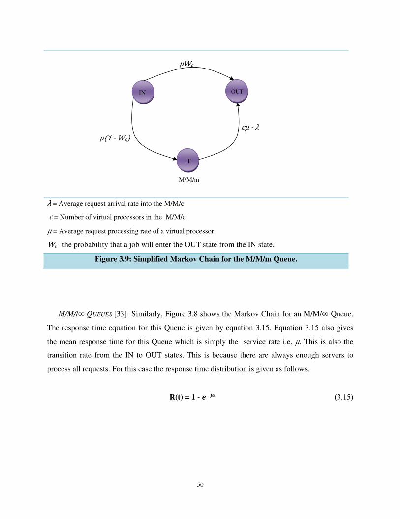
50
M/M// QUEUES [33]: Similarly, Figure 3.8 shows the Markov Chain for an M/M/ Queue.
The response time equation for this Queue is given by equation 3.15. Equation 3.15 also gives
the mean response time for this Queue which is simply the service rate i.e. . This is also the
transition rate from the IN to OUT states. This is because there are always enough servers to
process all requests. For this case the response time distribution is given as follows.
R(t) = 1 - (3.15)
= Average request arrival rate into the M/M/c
= Number of virtual processors in the M/M/c
= Average request processing rate of a virtual processor
= the probability that a job will enter the OUT state from the IN state.
Figure 3.9: Simplified Markov Chain for the M/M/m Queue.
IN
T
OUT
M/M/m

51
M/M/M QUEUES [33]: As shown in Figure 3.9, the M/M/m Queue can be modelled with three
states. As before, requests enter the IN state and as they complete processing, they enter the
OUT state. The T state represents a transient phase where requests can enter before completing.
This Markov Chain is derived from the response time equation [33] for the M/M/m Queue given
in equation 3.16.
R(t) = (3.16)
= Average request arrival rate into the M/M/c
= Number of virtual processors in the M/M/c
= Average request processing rate of a virtual processor
Equation 3.16 can be divided into two parts. An exponential part and a hypo-exponential part.
The exponential part is given by and the hypo-exponential part by
. Wc represents the probability of jobs
processed by the exponential part and intuitively, 1- Wc is the probability that jobs are processed
by the hypo-exponential part. Additionally it can be shown that from the exponential part, the
mean processing rate is µ. The hypo-exponential part has two sections, the first section also has a
mean processing rate of µ and the last section has a mean processing rate of, . c is the
number of servers/processors.
�
�
�
�
�

52
Based on equation 3.16 the transition rates of Figure 3.9 can be explained as follows: There is
a probability of Wc that requests entering the system will be completely processed at a rate of µ
and leave the system through the OUT state. Also there is a probability of that requests
entering the system will enter a transient T state at a rate of From this state they will be
completely services at a rate of and leave the system through the OUT state. The value
for [33] is calculated as shown in equation 3.4. Combining this probability with its respective
rate gives the actual transition rates. From IN to OUT, the transition rate is . Similarly, from
IN to T, the transition rate is .
The Markov Chains for the M/M/1, M/M/m and M/M/ Queues can be expressed in simpler
form as shown in Figures 3.8 and 3.9. These Markov Chains can be used as building blocks to
model much larger systems. As an example consider the Queuing Network of Figure 3.6. To
construct the Markov Chain assume that the web server is an M/M/m Queue, the database
servers are M/M/1 Queues and requests are entering the system from an M/M/ Queue.
Figure 3.10: Partial Markov Chain solution for the Queuing Network of Figure 3.6.
Only database 1 and the web server are represented.
d1 1
c 1 1
c 1 c
IN
OUT
OUT
T M/M/1
M/M/m
1 d1
c
c

53
The Markov Chain in Figure 3.10 shows how the M/M/m Queue (web server) is connected
to one of the M/M/1 Queue (database server), the other database server will be connected later.
The purple square to the right, represents the M/M/m Queue and the green rectangle represents
the M/M/1 Queue. The connections are dependent on the Queuing diagram of Figure 3.6 and the
Markov Chains for the M/M/1 and M/M/m Queues.
The M/M/1 Queue shares an IN state with the M/M/m Queue. Requests entering the M/M/m
Queue can either be completed with probability or enter the database at a rate of
. Notice that these rates differ from those shown in Figure 3.9. 1 and respectively has
Figure 3. 11: Complete Markov Chain solution for the Queuing Network of Figure 3.6.
IN
OUT
OUT
T
OUT

54
been added to the rates because these are the probabilities that a request will enter database 1 or
be completed as dictated by Figure 3.6.
Also according to Figure 3.6, requests processed at the database server will re-enter the
M/M/m Queus for further processing. This will happen at a rate of as shown in Figure 3.8.
The transient state T is also connected to the database. This is because a request that enters the
transient state for processing may end up requiring a database access before it can complete.
Based on Figure 3.8, requests will leave the transient state at a rate of . Also based on
Figure 3.6 the probability of entering database 1 is . Combining and gives the
actual rate at which requests are leaving the transient state of Figure 3.10, which is .
In Figure 3.11, database 2 is added using the same technique as before. An orange state has
also been added to account for the incoming request at a rate of , to the web server Queue. This
orange state model an M/M/ Queue and the service rate = processing rate i.e. . Figure
3.11 represents the complete Markov Chain for the Queuing Network shown in Figure 3.6.
Section 3.5 CONCLUSION
The three models of interest were described along with methods of calculating the
availability. Later in chapter 4 Markov Chains and fault Trees will be used to model both the
hardware and software systems in this research. Methods for solving continuous time Markov
Chains for both steady state and transient availabilities were demonstrated. Fault Trees were also
examined and techniques for calculating the availabilities were presented.
It was also shown how to significantly reduce the size of the Markov Chains for the M/M/1,
M/M/ M/M/m Queues. These Markov Chains were implemented with only two and three
states respectively and then used as building blocks to represent a large Queuing Network,

55
reducing the state space explosion problem. The method presented in Section 3.2, can then be
used to solve these Markov Chains for the transient probability that requests are completed by a
certain time. This is done by finding the response time equation for the absorbing state of the
Markov Chain. In chapter 4, three models will be combined in order to evaluate the availability
of virtual systems. This will be demonstrated by examining a small virtual cluster. The theory
and techniques presented in this chapter can be used to solve the combined model. For large
systems it will not be feasible to do this by hand and a computer program will be necessary. The
program used to solve the models in Chapter 4 is SHARPE [30].
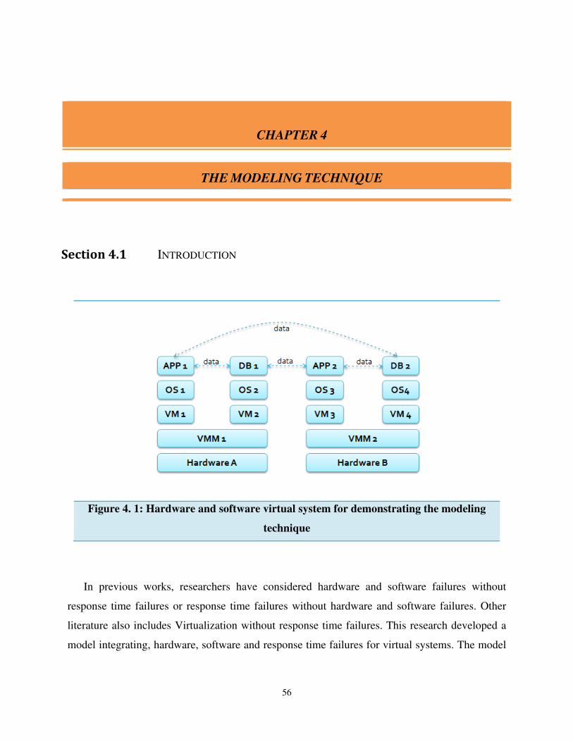
56
Section 4.1 INTRODUCTION
In previous works, researchers have considered hardware and software failures without
response time failures or response time failures without hardware and software failures. Other
literature also includes Virtualization without response time failures. This research developed a
model integrating, hardware, software and response time failures for virtual systems. The model
CHAPTER 4
THE MODELING TECHNIQUE
Figure 4. 1: Hardware and software virtual system for demonstrating the modeling
technique
57
incorporates failures due to inadequate processing power and multiple servers that need to
communicate with each other.
The modeling system will consist of two models: One of modeling response time failures
(sections 4.3 & 4.4) and the second for modeling hardware and software failures (section 4.2).
Both models are combined in section 4.5. Although the response time models are implemented
independently of the Fault Tree models the calculations do not assume independence. As will be
explained in the modeling steps, for every hardware and software configuration in the Fault Tree
model there is a corresponding response time model. Hence there is no assumption of
independence between these two models. Methods for finding the availability of the Fault Tree
and Markov Chain models were demonstrated in chapter 3. When evaluating larger systems, it is
more efficient to use a computer program to derive steady state and transient availabilities. The
program used in this chapter is SHARPE [30].
MODELING STEPS
A virtual system consists of many hardware and software systems working together. These
systems are normally constructed with redundancies, with each set of redundant component
performing the same job.
The modeling technique is completed by implementing the following steps:
1. Define what constitutes a full system failure.
− What is the minimum number of subsystems, required to be up for the system not to fail?
2. For a system with redundancies, determine the configurations that the system can be in
without experiencing a full system failure:
− For example consider a system with two virtual machines that are replicas of each
other: VM1, VM2.
58
− Define a full system failure as occurring only if all replicas fail.
− Possible configurations are:
o Both VM1 and VM2 are up,
o VM1is up and VM2 down,
o VM1 is down and VM2 is up.
3. For each configuration, construct a Fault Tree.
− This top level Fault Tree will be used to determine the probability of being in that
configuration.
4. For each component at the leaf of the Fault Tree construct a Markov Chain to compute
the steady state availability measures.
These measures are used as inputs into the Fault Tree leaves.
5. Construct Queuing Network models for each configuration to determine the probability
that requests are completed by a certain time.
Each configuration can have failed replicas and could therefore process requests at a
reduce rate. This can directly affect user perceived failures.
6. Convert each Queuing Network model to Markov Chains.
These Markov Chains are used to compute the probability that requests are completed by
a certain time.
7. Combine the results from the Queuing Network Models with their corresponding
hardware and software models to obtain the availability of the system.

59
This will be done by combining the probability of being in each configuration (step 3)
with the probability of request completing by a certain time (step 6).
DEMONSTRATION SYSTEM
Figure 4.1 describes the demonstration system which represents a small cluster at the IaaS
layer of the cloud. Application 1 (APP1) and Application 2 (APP2) both service server requests
from the same set. Some of these requests will require database access. All database accesses are
fulfilled by Database 1 (DB1) or Database 2 (DB2). The system of Figure 4.1 is implemented on
two hardware systems, Hardware A and Hardware B. Hardware A hosts Virtual Machine 1
(VM1), Operating System 1 (OS1), Application 1 (APP1) and Virtual Machine 2 (VM2),
Operating System 2 (OS2), Database 1 (DB1). Virtual Machine Monitor 1 (VMM1) manages
Hardware A resources. The setup is identical for the Hardware B system. In the next section the
modeling steps will be applied to the demonstration system.
Section 4.2 GENERATING THE FAULT TREE MODELS
T = (APP1.OS1.VM1.VMM1.HA). (APP2.OS3.VM3.VMM2.HB) . (DB1.OS2.VM2.VMM1.HA) . (DB2.OS4.VM4.VMM2.HB)
Figure 4. 2: Fault Tree for the hardware and software system represented by case 1.

60
STEP : 1 DEFINE WHAT CONSTITUTES A FULL SYSTEM FAILURE
The system of Figure 4.1 has two identical Application Servers and two identical Database
Servers. Define a full system failure as a failure that occurs when there isn’t at least one
application server together with one database server running.
STEPS 2 & 3: DETERMINE THE CONFIGURATIONS THAT THE SYSTEM CAN BE IN WITHOUT
EXPERIENCING A FULL SYSTEM FAILURE AND GENERATE THE FAULT TREES
Depending on the number of component failures, the system of Figure 4.1 can exist in nine
configurations where the system is still functional. For example, configuration 1 can be: All
components are fully functional. Configuration 2 can be: Only one application server is UP along
with the two databases. The Fault Tree models are used to compute the probability of being in
these types of configurations. Nine configurations or cases are examined.
Case 1:
Application 1 is UP, Application 2 is UP, Database 1 is UP, Database 2 is UP, Hardware A and
Hardware B are UP. The following shorter notation will be used hereafter:
(APP1 = UP, APP2 = UP, DB1 = UP, DB2 = UP, HA = UP, HB = UP)
APP1 = UP => APP1 AND OS1 AND VM1 AND VMM1 AND HA are all UP
APP2 = UP => APP2 AND OS3 AND VM3 AND VMM2 AND HB are all UP
DB1 = UP => DB1 AND OS2 AND VM2 AND VMM1 AND HA are all UP
DB2 = UP => DB2 AND OS4 AND VM4 AND VMM2 AND HB are all UP
Based on the above description, the equation, T which represents the Boolean equation for
the Fault Tree is given below.

61
T = (APP1.OS1.VM1.VMM1.HA) . (APP2.OS3.VM3.VMM2.HB) .
(DB1.OS2.VM2.VMM1.HA) . (DB2.OS4.VM4.VMM2.HB)
Note that a ‘.’ Is used to represent an AND gate and will later represent an OR gate by a ‘+’.
In Figure 4.2, the Fault Tree is given in case 1. This Fault Tree consists of multiple AND gates
and could be simplified to a single AND gate. The multiple AND gate structure is used for
demonstration purposes because it is easier to interpret the system architecture from that tree.
Case 2A:
Application 1 is UP, Application 2 is Down, Database 1 is UP, Database 2 is UP, Hardware A
and Hardware B are UP.
(APP1 = UP, APP2 =DOWN, DB1 = UP, DB2 = UP)
Boolean equation:
T = (APP1.OS1.VM1.VMM1.HA) . .
(DB1.OS2.VM2.VMM1.HA) . (DB2.OS4.VM4.VMM2.HB)
Note that APP2 can be down because OS3 fail OR VM3 fails OR APP2 fails. A failure in
VMM1 or HA could also trigger APP2 to fail but DB2 must be UP. Consequently VMM1 or HA
cannot fail in this case. Hence we derive the equation, . The FT for case
2A is demonstrated in Figure 4.3.
Case 2B:
(APP1 = DOWN, APP2 =UP, DB1 = UP, DB2 = UP)

62
T = . (APP2.OS3.VM3.VMM2.HB) .
(DB1.OS2.VM2.VMM1.HA) . (DB2.OS4.VM4.VMM2.HB)
The FT for case 2B is similar to case 2A.
Case 3A:
(APP1 = UP, APP2 =UP, DB1 = UP, DB2 = DOWN)
T = (APP1.OS1.VM1.VMM1.HA) .APP2.OS3.VM3.VMM2.HB) .
(DB1.OS2.VM2.VMM1.HA) .
The FT for case 2A is demonstrated in Figure 4.4.
T = (APP1.OS1.VM1.VMM1.HA) . (������������ +������� +���������) . (DB1.OS2.VM2.VMM1.HA) . (DB2.OS4.VM4.VMM2.HB)
Figure 4. 3: Fault Tree for the hardware and software system represented by case 2a.

63
Case 3B:
(APP1 = UP, APP2 =UP, DB1 = DOWN, DB2 = UP )
T = (APP1.OS1.VM1.VMM1.HA).(APP2.OS3.VM3.VMM2.HB) .
. (DB2.OS4.VM4.VMM2.HB)
The FT for case 3B is similar to case 3A.
Case 4A:
(APP1 = UP, )
T = (APP1.OS1.VM1.VMM1.HA) .APP2.OS3.VM3.VMM2.HB) . (DB1.OS2.VM2.VMM1.HA) . (��������� +�������� +����������)
Figure 4. 4: Fault Tree for the hardware and software system represented by case 3A.

64
T = (APP1.OS1.VM1.VMM1.HA) . .
(DB1.OS2.VM2.VMM1.HA).
The FT for case 4A is similar is shown in Figure 4.5.
Case 4B:
(APP1 = UP, , D1 = DOWN, )
T = (APP1.OS1.VM1.VMM1.HA) . . .
(DB2.OS4.VM4.VMM2.HB)
The FT for case 4B is similar is shown in Figure 4.6.
T = (APP1.OS1.VM1.VMM1.HA) . (������������ +������� +��������� + ������������� +������) . (DB1.OS2.VM2.VMM1.HA). (��������� +�������� +���������� +������������� + ������)
Figure 4. 5: Fault Tree for the hardware and software system represented by case 4A.

65
Case 4C:
(APP1 = DOWN, )
T = . (APP2.OS3.VM3.VMM2.HB) .
(DB1.OS2.VM2.VMM1.HA) .
The FT for case 4C is similar to case 4B.
Case 4D:
(APP1 = DOWN, )
T = . (APP2.OS3.VM3.VMM2.HB)
. . (DB2.OS4.VM4.VMM2.HB)
The FT for case 4D is similar to case 4A.
T = (APP1.OS1.VM1.VMM1.HA) . (������������ +������� +���������) . (��������� +�������� +����������) . (DB2.OS4.VM4.VMM2.HB)
Figure 4. 6: Fault Tree for the hardware and software system represented by case 4A.

66
The Boolean equations for the following groups of cases are very similar. Cases 2A & 2B,
3A & 3B, 4A &4D and 4B & 4C. Since components, such as APP1, APP2 are replicas of each
other, these groups of equations produce the same results.
STEPS 4: FOR EACH COMPONENT AT THE LEAF OF THE FAULT TREE CONSTRUCT A MARKOV
CHAIN TO COMPUTE THE STEADY STATE AVAILABILITY MEASURES.
The leaves of the Fault Trees, which are represented as the variables in the Fault Tree
equations will now be examined. HA & HB leaves, are implemented as shown in Figure 4.7. The
leaves of the Figure 4.7 gate are implemented as Markov Chains as described in [15]. The
Markov Chains for Power supply (POW), Data Storage (Hdd), Memory (MEM),Processor
(CPU) and Network system (NET) are given in [15] in figures 5, 8, 4, 3 and 6 respectively.
The same type of Markov Chain for APP, DB, OS, VM and VMM is used in this research.
This Markov Chain was adapted from [15] and shown in Figure 4.8 of this thesis. The rates for
each system (APP, DB, OS, VM and VMM) are given in Table 4.1.
The steady state probability of being UP or DOWN for the leaves of the Fault Trees (ex.
APP1, DB1, OS1, VM1, VMM1, HA) are derived from the Markov Chains for that leaf. For a
barred leaf, example, the probability of being DOWN (steady state unavailability) is fed
Figure 4.7: Fault Tree for generating Hardware A or B probabilities
OR
POW Hdd MEM CPU NET
HA or HB

67
into the gate. For a non-barred leaf, example, APP1, the probability of being UP (steady state
unavailability) is fed into the gate. Assume that both APPs, both DBs, all OSs, all VMs, all
VMMs and both hardware systems are all replicas and behave the same way, sharing the same
rates.
The Markov Chain of Figure 4.8 represents the systems, APP, DB, OS, VM and VMM with
their respective rates shown in Table 4.1. The chain starts in the UP state and can go down (DN)
at a rate of λy. From the DN state the system can be rebooted and returns to the UP state at a rate
of byβy. It can fail to reboot and remain down (DW state). From the DW state a repair person is
called at a rate of αy and the system goes to the repair state RP. From the RP state it is repaired at
a rate of µy and returns to the UP state.
TABLE 4. 1: Rates for the Markov Chain of Figure 4.8. The rates are for 4 different systems: Application
APP, VM, OS and the VMM.
Symbol VM APP/DB OS VMM
1/λY : mean time for failure 2880 hrs 336 hrs 1440 hrs 2880 hrs
1/δY : mean time for failure detection
30 sec 30 sec 30 sec 30 sec
1/µY: mean time for repair 30 min 30 min 1 hr 1 hr
1/βY: mean time to restart
5 min 5 min 5 min 5 min
1/αY: mean time to for repair person arrival 30 min 30 min 30 min 30 min
1/bY: Probability that restart is successful 0.9 0.9 0.9 0.9

68
Section 4.3 QUEUING NETWORK MODELS
STEPS 5: CONSTRUCT QUEUING NETWORK MODELS FOR EACH CONFIGURATION TO DETERMINE
THE PROBABILITY THAT REQUESTS ARE COMPLETED BY A CERTAIN TIME.
Case 1: Both applications and both databases are up. This configuration is demonstrated by
the Queuing Network in Figure 4.9. Requests enter the system at a rate of λ and are distributed
among VM1 and VM3. After processing by VM1 and VM3, some requests will be fully serviced
and complete with probability, Xc or enter VM2 (A database request) with probability X1 or VM4
(A database request) with probability X2. After leaving the databases these requests will re-enter
VM1 or VM3.
The rates at which requests enter VM1, VM3, VM2 AND VM4 are given by λ1, λ2, λd1 and
λd2 respectively. These variables are solved by deriving the simultaneous traffic equations for the
Queuing Network as demonstrated in chapter 3. The traffic equations for Case 1 are given by:
1 = Xc + X1 + X2
Figure 4.8: Case 1: Both applications and both Databases are UP
Application 1 on VM1
Database 1 on VM2
λ
µ1
µ2
µ1
Application 2 on VM3
µ3
Database 2 on VM3

69
λ1 = λ /2 + (λd1 + λd2)/2 ,
λ2 = λ /2 + (λd1 + λd2)/2
λd1 = X1(λ1 + λ2) ,
λd2 = X2(λ1 + λ2)
Case 2A or 2B: One application is UP and both Databases are UP. The Queuing Network for
this system is given in Figure 4.10. These cases have the same Queuing Network and the
performance model. The traffic equations for Case 2A or 2B are given by:
1 = Xc + X1 + X2
λ1 = λ + (λd1 + λd2)
λd1 = X1(λ1),
λd2 = X2(λ1)
Case3A or 3B: Both applications are UP and only one database is UP. These cases share the
same Queuing Network and the performance model. The Queuing Network for this system is
given in Figure 4.11. The traffic equations for Case 3A or 3B are given by:
1 = Xc + X1
λ1 = λ /2 + λd1/2 ,
λ2 = λ /2 + λd1/2 ,
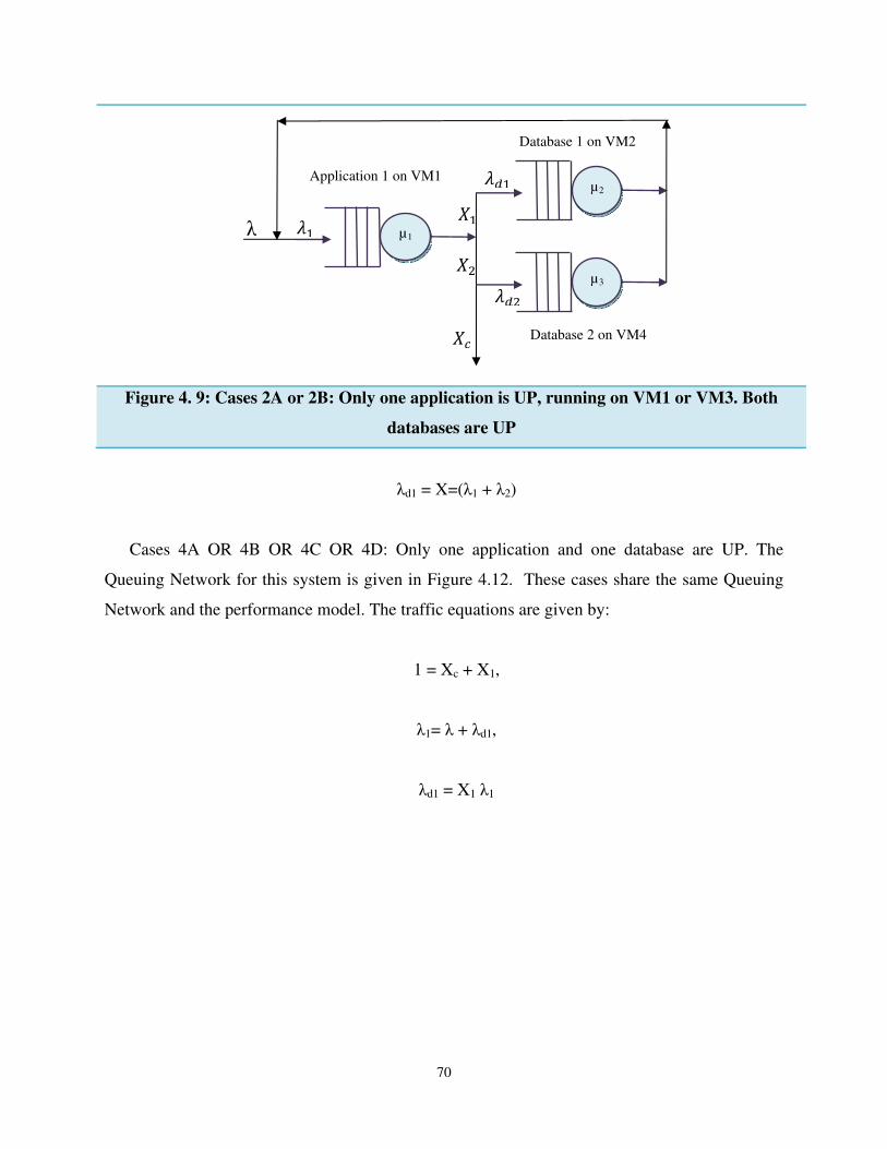
70
Figure 4. 9: Cases 2A or 2B: Only one application is UP, running on VM1 or VM3. Both
databases are UP
λd1 = X=(λ1 + λ2)
Cases 4A OR 4B OR 4C OR 4D: Only one application and one database are UP. The
Queuing Network for this system is given in Figure 4.12. These cases share the same Queuing
Network and the performance model. The traffic equations are given by:
1 = Xc + X1,
λ1= λ + λd1,
λd1 = X1 λ1
Database 1 on VM2
λ
µ1
µ2
µ3
Application 1 on VM1
Database 2 on VM4
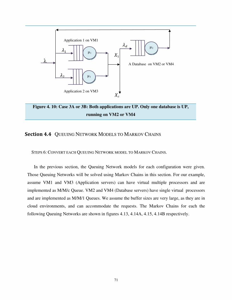
71
Section 4.4 QUEUING NETWORK MODELS TO MARKOV CHAINS
STEPS 6: CONVERT EACH QUEUING NETWORK MODEL TO MARKOV CHAINS.
In the previous section, the Queuing Network models for each configuration were given.
Those Queuing Networks will be solved using Markov Chains in this section. For our example,
assume VM1 and VM3 (Application servers) can have virtual multiple processors and are
implemented as M/M/c Queue. VM2 and VM4 (Database servers) have single virtual processors
and are implemented as M/M/1 Queues. We assume the buffer sizes are very large, as they are in
cloud environments, and can accommodate the requests. The Markov Chains for each the
following Queuing Networks are shown in figures 4.13, 4.14A, 4.15, 4.14B respectively.
Figure 4. 10: Case 3A or 3B: Both applications are UP. Only one database is UP,
running on VM2 or VM4
Application 1 on VM1
A Database on VM2 or VM4
λ
µ1
µ2
µ1
Application 2 on VM3

72
Figure 4. 11: Cases 4A OR 4B OR 4C OR 4D: Only one application is UP, running on
VM1 or VM3. One database is UP running on VM2 or VM4
They are all constructed in a similar way as demonstrated in chapter 3. A detailed explanation of
the more complicated case 1 (Figure 4.13) will be given. From chapter 3, an M/M/m Queue can
be represented by three states. Therefore VM1 and VM3 are implemented with three states. For
VM1 the three states in Figure 4.13 are VM1_1, VM1_2 and the C state. The C state is an
absorbing state that is used to calculate the probability of a request completing. For each Markov
Chain the following variables are defined:
• C1 and C2 = number of virtual CPUs, for VM1 &VM3,
• U1, U2, Ud1, Ud2 = Processing speed of each virtual CPU for VM1, VM3, VM2, &
VM4 respectively,
• Wc= Constant calculated from equation 3.16,
• λ1, λ2, λd1, λd2, X1, X2 and Xc are calculated from the traffic equations in the previous
section.
Application 1 on VM1
A Database on VM2 or VM4
λ
µ1
µ2
An application on VM1 or VM3
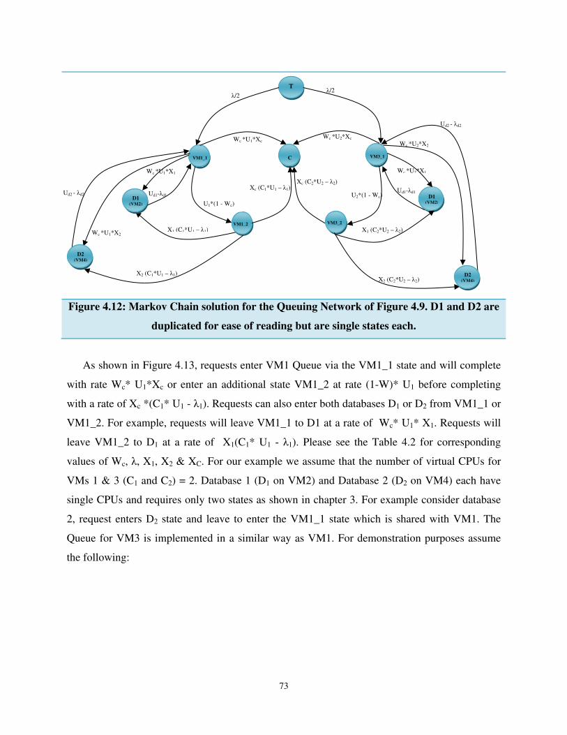
73
As shown in Figure 4.13, requests enter VM1 Queue via the VM1_1 state and will complete
with rate Wc* U1*Xc or enter an additional state VM1_2 at rate (1-W)* U1 before completing
with a rate of Xc *(C1* U1 - λ1). Requests can also enter both databases D1 or D2 from VM1_1 or
VM1_2. For example, requests will leave VM1_1 to D1 at a rate of Wc* U1* X1. Requests will
leave VM1_2 to D1 at a rate of X1(C1* U1 - λ1). Please see the Table 4.2 for corresponding
values of Wc, λ, X1, X2 & XC. For our example we assume that the number of virtual CPUs for
VMs 1 & 3 (C1 and C2) = 2. Database 1 (D1 on VM2) and Database 2 (D2 on VM4) each have
single CPUs and requires only two states as shown in chapter 3. For example consider database
2, request enters D2 state and leave to enter the VM1_1 state which is shared with VM1. The
Queue for VM3 is implemented in a similar way as VM1. For demonstration purposes assume
the following:
Figure 4.12: Markov Chain solution for the Queuing Network of Figure 4.9. D1 and D2 are
duplicated for ease of reading but are single states each.
Ud2 - λd2
Ud2 - λd2
Ud1-λd1
Xc (C1*U1 – λ1)
X1 (C1*U1 – λ1)
Wc *U1*X1
Wc *U1*Xc
VM1_1
C
VM1_2
U1*(1 - Wc)
T
Wc *U1*X2
X2 (C1*U1 – λ1)
λ/2
Ud1-λd1
X1 (C2*U2 – λ2)
Wc *U2*X1
Wc *U2*Xc
VM3_1
D1 (VM2)
VM3_2
U2*(1 - Wc)
Wc *U2*X2
X2 (C2*U2 – λ2)
λ/2
Xc (C2*U2 – λ2)
D1 (VM2)
D2 (VM4)
D2 (VM4)

74
Virtual CPU speed for U1 (VM1), U2 (VM3), Ud1 (VM2), Ud2 (VM4) = 1000 GHz
Avg. number of cycles per instruction = 4;
Avg. number of instruction/requests per hour =
( ) * 120 = 30,000* 109
Hence ‘µ’, the processing rate for each virtual CPU = 30,000* 109 requests/hr. The method
developed in [33] is used to calculate Wc, for VMs 1 & 2 and is given in chapter 3. All the
parameters in the Markov Chains can be modified for other systems. In figures 4.13 and 4.15
there are multiple D1 and D2 states but actually represent single states each. This was done to
reduce the crossing of arcs so that the chains can be read easily.
In order to solve the Markov Chains, Wc is calculated, all λ’s are calculated from the
respective traffic equations and are given in Table 4.3. X1 & X2 are calculated from the equations
in the previous section and are given in Table 4.2. Recall that Xc is the probability that requests
are completed, X1 & X2 are the probabilities that requests will enter database 1 or 2 respectively.
TABLE 4. 2:Column 2: Fault Tree availability for each case. Column 3: Probability that
requests is completed in the Queuing Network. The total request arrival rate λ, the
constant W from eq. 1 & the probability that requests are completed, Xc are also given.
Fault Tree Queuing net. λ W Xc X1 X2
Steady State
Availability
Probability to
complete within
100ms
(109)
Case 1 0.99078962 0.89932725
3000 0.9967 0.6 0.2 0.2
Case 2A,B 0.00201139 0.681096696
3000 0.9873 0.6 0.2 0.2
Case 3A,B 0.00201139 0.899247014
3000 0.9967 0.6 0.4
Case 4A,D 0.00018184 0.680866086
3000 0.9873 0.6 0.4
Case 4B,C 0.00000408 0.680866086
3000 0.9873 0.6 0.4
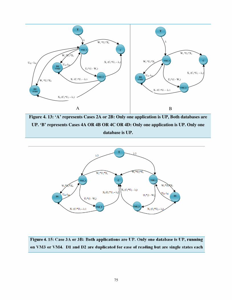
75
A
B
Figure 4. 13: ‘A’ represents Cases 2A or 2B: Only one application is UP, Both databases are
UP. ‘B’ represents Cases 4A OR 4B OR 4C OR 4D: Only one application is UP. Only one
database is UP.
Ud1-λd1
Xc (C1*U1 – λ1)
X1 (C1*U1 – λ1)
Wc *U1*X1
Wc *U1*Xc
VM1_1
C
VM1_2
U1*(1 - Wc)
T
λ
D1 (VM2)
Ud2 - λd2
λ
Ud1-λd1
Xc (C1*U1 – λ1)
X1 (C1*U1 – λ1)
Wc *U1*X1
Wc *U1*Xc
VM1_1
C
VM1_2
U1*(1 - Wc)
T
Wc *U1*X2
X2 (C1*U1 – λ1)
D1 (VM2)
D2 (VM4)

76
Section 4.5 COMBINING THE DATA FROM FAULT TREE AND QUEUING NETWORK
MODELS
STEPS 7: COMBINE THE RESULTS FROM THE QUEUING NETWORK MODELS WITH THEIR
CORRESPONDING HARDWARE AND SOFTWARE MODELS TO OBTAIN THE AVAILABILITY OF THE
SYSTEM.
For the Fault Tree, the probability of the system being in a configuration, given by cases 1 to
4 is obtained by evaluating the Fault Tree equations as demonstrated in chapter 3. In this section
the evaluation was done by using the SHARPE package [30]. Column 2 of Table 4.2 gives the
steady state probability that the system will be in each case. For example, the steady state
probability that the system will be in configuration given by case 2A is 0.00201139. For each
equivalent case in the Queuing Networks, the probability that requests are completing by a
certain time is evaluated by calculating the transient probability of reaching ‘C’ (completion state
) of the Markov Chains (figures 4.13 – 4.15).
All Markov Chains are also solved using the SHARPE software [30]. Column 3 of Table 4.2
gives the probability that requests entering the Markov Chains, from state T will be completed by
100ms. For case 2A that probability is 0.681096696. This probability is obtained from the
Markov Chains representing case 2A, shown in Figure 4.14A.
TABLE 4. 3: Arrival rates for each Queuing Network & related Markov Chain.
λ (109) λ1 (109) λ2 (109) λd1 (109) λd2 (109)
Case 1 3000 2500 2500 1000 1000
Case 2 (A, B) 3000 5000 1000 1000
Case 3 (A, B) 3000 2500 2500 2000
Case 4 (A, B, C, D) 3000 5000 2000

77
EVALUATION WITHOUT INCLUDING RESPONSE TIMES
The availability of the system without response time failures = Sum of all availabilities for each
case in the Fault Tree model.
From Table 2 col.2 system availability,
Asys= 0.99078962 + 2 * 0.00201139 + 2 * 0.00201139 + 2 * 0.00018184 + 2 * 0.00000408
Asys = 0.99920702
A multiplication factor of 2 is used where two cases produce the same result.
EVALUATION INCLUDING RESPONSE TIMES
The availability of the system with response time failures = Sum (Availability for each case in
the response time model * the probability of the equivalent FT model).
Asys= 0.89932725 *(0.99078962) + 0.681096696 *(2 * 0.00201139) + 0.899247014 *
(2 * 0.00201139) + 0.680866086 *(2 * 0.00018184) + 0.680866086 *(2 * 0.00000408)
Asys = 0.89765465
Section 4.6 CONCLUSION
A modeling system that combined Queuing Networks, Markov Chains and Fault Trees was
presented for evaluating the availability of virtual systems. The model was demonstrated on a
small virtual cluster. The evaluation was done for the system in two ways:
78
1 ) Without considering response time failures and
2) With response time failures included.
In chapter 5, the results obtained here will be explained in more details along with a conclusion
and recommendations for future work.
79
Section 5.1 SUMMARY OF THE MODELING TECHNIQUE
In Chapter 4, the techniques used to model virtual and cloud systems was explained and
demonstrated using a small cluster as an example. The cluster was divided up into nine
configurations and further organized into four different cases. Each configuration represented a
possible partially functioning state that the cluster could be in. In a partially functioning state the
cluster has failed components but can still service requests. For example, the cluster has two
identical web servers, if one fails the other can still carry out the required function but with
degraded performance.
Fault trees were used to compute the probability of the system being in any of the nine
configurations for each of the four cases. Since each of the nine configurations has failed
components, a performance model using queuing networks was constructed for each
configuration. The queuing network was then used to compute the probability of requests coming
into the system completing by a certain time. For the demonstration system in Chapter 4, the
probability of requests completing, was evaluated at 100ms.
Section 5.2 CONCLUSION
SYSTEM AVAILABILITY
Using the Fault trees, the probability of the system being in a particular operational/UP
configuration was computed, rather than having one Fault trees to compute a full system failure
CHAPTER 5
CONCLUSION AND FUTURE WORK

80
as in previous works. It was not assumed that the hardware/software model is independent of the
response time model as in other literatures.
• Based on the calculations from Chapter 4, section 4.5, the system availability when
response time is incorporated is 0.89765465. When response time is not incorporated, it is
0.99920702 which is higher. The availability with response time incorporated is a more
practical evaluation of the system.
• Based on the Fault tree probabilities, the system will rarely be in any configuration other
than case 1 (col 2 Table 4.2). Other cases have a prob. <0.00202.
• It can be deduced that for this system with a processing rate of 30,000*109, two databases
are not necessary. This is because, both case 1 and case 3 produce almost the same
response time probabilities (col. 4.3 Table II). If the system was more loaded, the two
databases may be necessary.
Table 5. 1: Comparative Table showing a summary of the results
obtained from chapters 4 and 5.
` Without
Response Time
Failures
With Response
Time Failures
System
Availability
0.99920702
0.89765465
Down Times
Over a 1 year
period
2 days
38 days

81
DOWNTIMES:
Another useful way of evaluating the system is to calculate its average downtime. First the
downtime is calculated for the system without response time measures and then with response
times.
WITHOUT RESPONSE TIME
Without response time failures, as shown in Chapter 4 Table 4.2, the probability of being in a
fully functional system, given by case 1, which is: 0.99078962. The probability of being in any
of the other configurations: 1 - 0.99078962 = 0.00921038
It is known that cases 3a and 3b will perform approximately the same as the fully functional
state as shown in Table 4.2. If the probabilities for 3a and 3b are now removed, what is left is the
probability that the system will be in a poorly performing, non-useful state.
Remove Case 3a and 3b: 0.00921038 – 2 * 0.00201139 = 0.0051876.
For a period of a year, the system will be down in a poorly performing state for an average of
approximately 2 days. i.e. Downtime = 365 * 0.0051876 2 days.
WITH RESPONSE TIME
With response time failures, as shown in Chapter 4 Table 4.2, the probability of being in a
fully functional system, given by case 1. Fully functional system is 0.99078962* 0.89932725 =
0.8910441. Where 0.89932725 is the probability that requests are completed by 100ms. The
probability of being in any of the other configurations: 1 - 0.8910441 = 0.1089559.
Again, it is known that cases 3a and 3b will perform approximately the same as the fully
functional state as shown in Table 4.2. If the probabilities for 3a and 3b are now removed, what
is left is the probability that the system will be in a poorly performing, none useful state. Remove

82
Case 3a and 3b: 0.1089559 – 2 * 0.00201139*0.899247014 = 0.10533842. Where 0.899247014
is the probability that requests are completed by 100ms.
For a period of a year, the system will be down in a poorly performing state for an average of
approximately 38 days. i.e. Downtime = 365 * 0.003617473 38 days
When response times are taken into consideration, the system performs poorly for 38 days out of
1 year. This estimate is based on the requirement that requests must be completed by 100ms. If
this number was increased then the downtimes would decrease from 38 days.
An integrated modeling technique was developed to assess hardware, software and response
time failures in clouds and other systems based on Virtualization. The modeling system supports
networks where requests need to be passed to multiple servers. Figure 4.9 gives an example
where a request is processed at the application server then passed to the database server and
return to the application server for completion. The modeling technique makes it possible to
vary the number of processors and the processing rates of the servers allowing the evaluation of
sharing or consolidating hardware resources. The models can also be used to evaluate the system
for different request rates and at different time periods, different hardware and different VM
configurations. The model can also be evaluated for other measures such as average utilization of
the virtual CPUs and bottlenecks.
As shown in Table 5.1, when response times are not considered the results can be misleading.
In fact, when response times (evaluated at 100ms for the completion of requests) are
incorporated, the average downtime were 36 days higher for a period of one year which is very
significant. A system cannot be considered to be up in the traditional way by saying that it is up
if the hardware and software systems are up. A systems hardware and software can be up but the
response times can be low and the user will not see requests completing on time and perceive
that as a failure, this is especially true for time critical systems. In principle the modeling
technique can be applied to any hardware and software system in which response times play an
important role.

83
Section 5.3 FUTURE WORK
Another key issue in cloud computing is migration. This research continues with evaluating a
model having features similar to this one and capable of integrating migration and response time
failures. The new model will be used to evaluate migration policies and how they affect the
availability of the virtual system.

84
BIBLIOGRAPHY
[1] T. Abels, P. Dhawan and B. Chandrasekaran, "An overview of Xen virtualization," Dell
Inc, 2005.
[2] S. Amari, G. Dill and E. Howald, "A new approach to solve dynamic fault trees," in
Reliability and Maintainability Symposium, 2003. Annual, 2003, pp. 374-379.
[3] Amazon, "Amazon elastic compute cloud: User Guide," Amazon Web Services, Internet:
http://docs.huihoo.com/kvm/kvm-white-paper.pdf, 2012.
[4] M. Assuncao, A. di Costanzo and R. Buyya, "Evaluating the cost-benefit of using cloud
computing to extend the capacity of clusters," in Proceedings of the 18th ACM
International Symposium on High Performance Distributed Computing, Garching,
Germany, 2009, pp. 141-150.
[5] G. Bolch, S. Greiner, H. d. Meer and K. S. Trivedi, Queueing Networks and Markov
Chains. Wiley-Interscience, 2005.
[6] T. Bonald, "Insensitive queueing models for communication networks," in Proceedings
of the 1st International Conference on Performance Evaluation Methodolgies and Tools,
Pisa, Italy, 2006.
[7] R. Buyya, J. Broberg and A. M. Goscinski, Cloud Computing Principles and Paradigms.
Wiley Publishing, 2011.
[8] J. Che, T. Zhang, W. Lin and H. Xi, "A markov chain-based availability model of virtual
cluster nodes," in Computational Intelligence and Security (CIS), 2011 Seventh
International Conference on, 2011, pp. 507-511.
[9] S. Distefano and A. Puliafito, "Dependability modeling and analysis in dynamic
systems," in Parallel and Distributed Processing Symposium, 2007. IPDPS 2007. IEEE
International, 2007, pp. 1-8.
[10] S. Distefano and A. Puliafito, "Dynamic reliability block diagrams VS dynamic fault
trees," in Reliability and Maintainability Symposium, 2007. RAMS '07. Annual,2007, pp.
71-76.
85
[11] R. Figueiredo, P. A. Dinda and J. Fortes, "Guest Editors' Introduction: Resource
Virtualization Renaissance," Computer, vol. 38, pp. 28-31, 2005.
[12] I. Foster, Y. Zhao, I. Raicu, S. Lu, "Cloud Computing and Grid Computing 360-Degree
Compared," Grid Computing Environments Workshop, 2008. GCE '08 , pp.1-10, 12-16
Nov. 2008
[13] Google “An overview of Google Docs,” Internet:
http://support.google.com/docs/bin/answer.py?hl=en&answer=49008, 2012
[14] M. Kaniche, K. Kanoun and M. Martinello, "A user-perceived availability evaluation of a
web based travel agency," in Dependable Systems and Networks, 2003. Proceedings.
2003 International Conference on, 2003, pp. 709-718.
[15] D. Kim, F. Machida and K. S. Trivedi, "Availability modeling and analysis of a
virtualized system," in Dependable Computing, 2009. PRDC '09. 15th IEEE Pacific Rim
International Symposium on, 2009, pp. 365-371.
[16] D. Kondo, B. Javadi, P. Malecot, F. Cappello and D. P. Anderson, "Cost-benefit analysis
of cloud computing versus desktop grids," in Parallel & Distributed Processing, 2009.
IPDPS 2009. IEEE International Symposium on, 2009, pp. 1-12.
[17] X. Li, Y. Li, T. Liu, J. Qiu and F. Wang, "The method and tool of cost analysis for cloud
computing," in Cloud Computing, 2009. CLOUD '09. IEEE International Conference on,
2009, pp. 93-100.
[18] F. Machida, Dong Seong Kim and K. S. Trivedi, "Modeling and analysis of software
rejuvenation in a server virtualized system," in Software Aging and Rejuvenation
(WoSAR), 2010 IEEE Second International Workshop on, 2010, pp. 1-6.
[19] V. Mainkar, "Availability analysis of transaction processing systems based on user-
perceived performance," in Reliable Distributed Systems, 1997. Proceedings, the
Sixteenth Symposium on, 1997, pp. 10-17.
[20] R. Manian, D.W. Coppit, K.J. Sullivan and J. B. Dugan, "Bridging the gap between
systems and dynamic fault tree models," Reliability and Maintainability Symposium,
1999. Proceedings. Annual, pp.105-111, 18 -21 Jan 1999
[21] Microsoft, "Microsoft office 365 data sheet," Microsoft Corporation, Internet:
http://www.atea.se/media/69972/microsoft_office_365_for_midsized_businesses.pdf,
2010.

86
[22] M. Myint and T. Thein, "Availability improvement in virtualized multiple servers with
software rejuvenation and virtualization," in Secure Software Integration and Reliability
Improvement (SSIRI), 2010 Fourth International Conference on, 2010, pp. 156-162.
[23] Oracle, "Oracle VM VirtualBox user manual," Oracle Corporation, Internet:
http://download.virtualbox.org/virtualbox/UserManual.pdf, 2011.
[24] R. Paharsingh and O. Das, "An availability model of a virtual TMR system with
applications in Cloud/Cluster computing," in High-Assurance Systems Engineering
(HASE), 2011 IEEE 13th International Symposium on, 2011, pp. 261-268.
[25] R. Paharsingh and O. Das, "Availability analysis in virtual systems, with applications in
cloud computing," in 2nd International Workshop on Cloud Computing and Scientific
Applications (CCSA 2012), Ottawa, Canada, 2012.
[26] R. Prodan, M. Sperk and S. Ostermann, "Evaluating High-Performance Computing on
Google App Engine," Software, IEEE, vol. 29, pp. 52-58, 2012.
[27] Qumranet, "KVM: Kernel-based virtualization driver," Qumranet Inc., Internet:
http://docs.huihoo.com/kvm/kvm-white-paper.pdf, 2006.
[28] H. V. Ramasamy and M. Schunter, "Architecting dependable systems using
virtualization," in In Workshop on Architecting Dependable Systems in Conjunction with
2007 International Conference on Dependable Systems and Networks (DSN-2007, 2007).
[29] A. Rezaei and M. Sharifi, "Rejuvenating high available virtualized systems," in
Availability, Reliability, and Security, 2010. ARES '10 International Conference on,
2010, pp. 289-294.
[30] R. Sahner Sahner, K. S. Trivedi and A. Puliafito, “Performance and Reliability Analysis
of Computer Systems: An Example-Based Approach using the SHARPE Software
Package”, Norwell, MA, USA: Kluwer Academic Publishers, 1996.
[31] W. E. Smith, K. S. Trivedi, L. A. Tomek and J. Ackaret, "Availability analysis of blade
server systems," IBM Systems Journal, vol. 47, pp. 621-640, 2008.
[32] T. Thein, M. Pokharel, S. Chi and J. Park, "A recovery model for survivable distributed
systems through the use of virtualization," in Networked Computing and Advanced
Information Management, 2008. NCM '08. Fourth International Conference on, 2008, pp.
79-84.

87
[33] K. S. Trivedi, Probability and Statistics with Reliability, Queuing and Computer Science
Applications. Chichester, UK: John Wiley and Sons Ltd, 2002.
[34] I. Trummer, F. Leymann, R. Mietzner and W. Binder, "Cost-optimal outsourcing of
applications into the clouds," in Cloud Computing Technology and Science (CloudCom),
2010 IEEE Second International Conference on, 2010, pp. 135-142.
[35] L. M. Vaquero, L. Rodero-Merino, J. Caceres and M. Lindner, "A break in the clouds:
towards a cloud definition," SIGCOMM Comput.Commun.Rev., vol. 39, pp. 50-55,
December, 2008.
[36] VMware, "The architecture of VMware ESXi," VMware Inc., Internet:
http://www.vmware.com/files/pdf/ESXi_architecture.pdf, 2008.
[37] VMware, "VMware server User’s guide," VMware Inc., Internet:
http://www.vmware.com/products/beta/vmware_server/vmserver2.pdf, 2008.
[38] VMware, "Using VMware workstation," VMware Inc., Internet:
http://www.vmware.com/pdf/ws80-using.pdf, 2011.
[39] VMware, "Understanding full virtualization, paravirtualization, and hardware assist,"
VMware Inc., Internet:
http://www.vmware.com/files/pdf/VMware_paravirtualization.pdf, 2007.
[40] D. Wang and K. S. Trivedi, "Modeling user-perceived service availability," in
Proceedings of the Second International Conference on Service Availability, Berlin,
Germany, 2005, pp. 107-122.
[41] B. Wei, C. Lin and X. Kong, "Dependability modeling and analysis for the virtual
clusters," in Computer Science and Network Technology (ICCSNT), 2011 International
Conference on, 2011, pp. 2316-2320.
[42] J. Xiaojing, "Google cloud computing platform technology architecture and the impact
of its cost," in Software Engineering (WCSE), 2010 Second World Congress on, 2010,
pp. 17-20.
[43] T. Zheng and M. Woodside, "Fast estimation of probabilities of soft deadline misses in
layered software performance models," in Proceedings of the 5th International Workshop
on Software and Performance, Palma, Illes Balears, Spain, 2005, pp. 181-186.

88
[44] M. Zhou, R. Zhang, D. Zeng and W. Qian, "Services in the cloud computing era: A
survey," in Universal Communication Symposium (IUCS), 2010 4th International, 2010,
pp. 40-46.

89
ABBREVIATIONS
VMM Virtual Machine Monotor
VM Virtual Machine
IaaS Infrastructure as a Service
PaaS Platform as a Service
SaaS Software as a Service
RBD Reliability Block Diagram
LQN Layered Queuing Networks
QN Queuing Networks
MC Markov Chain
FT Fault Tree
FCFS First-Come-First-Served
LCFS Last-Come-First-Served
RR Round Robin
APP1 Application 1
APP2 Application 2
DB1 Database 1
DB2 Database 2
HA Hardware A
HB Hardware B