Auxiliary-field quantum Monte Carlo for correlated electron systems

Shiwei Zhang [shiwei@wm.edu]College of William & Mary, Virginia, USA

Outline• Interacting quantum matter -- a grand challenge need methods with: accuracy, computational scaling

• A general framework for correlated electron systems: Constrained path (phase-free) AFQMC

An ``emergent’’ of independent-electron solutions How does the sign problem occur? How to control it?

• Applications Hubbard models/optical lattice both molecules and solids

Labs

• Lab 1: Jie Xu, Huy Ngyen, Hao Shi, SZ Matlab code (more direct and interactive, slow!) Fermi Hubbard model exercises range from basic exploration to advanced additions to

the code (optional)

• Lab 2: Wirawan Purwanto, SZ C++ code Bose Hubbard model: AFQMC for trapped bosons exercises range from basic to advanced

Packages for both Labs at http://www.democritos.it/montecarlo2012/index.php/Main/Program

Revised version of Lab 1 will be available: physics.wm.edu/~shiwei

Collaborators: – Wissam Al-Saidi (Pittsburgh)– Chia-Chen Chang (UC Davis)– Simone Chiesa– Henry Krakauer– Wirawan Purwanto– Hao Shi– Jie Dorothy Xu (Citi Group)– Fengjie Ma – Yudis Virgus

Support:– NSF: electronic structure; method development– DOE ThChem: quantum chemistry – DOE SciDAC (UIUC, W&M, Princeton); DOE cmcsn network

(Cornell, W&M, Rice, LLNL)– Computing: DOE INCITE (Oak Ridge) and NSF Blue Waters (UIUC)

The electronic problem ‘Simple’ theory --- Schrödinger Eq:

with

MnO

H� = E�

Why hard?

riA major success in physics: --> Vint Vmf

e.g. Density functional theory

because is not separable! ( ...)Vint �i

“Bread and butter” calculations

• Density functional theory (DFT) with local-density types of approximate functionals: LDA, GGA, ….

• Independent-electron framework

LDA

H2 ��

i

fc(ni)niLDA:

c†i c†jckcl � ⇥c†i cl⇤c†jck + · · ·HF:

H =M�

i,j

Tij c†jcj +M�

i,j,k,l

Vijklc†i c

†jckcl

• In 2nd quantization: ABINIT, ESPRESSO, VASP,

GAMESS, Gaussian, ….

�i

Can always solve 1-body problem: (e.g., grid, Gaussians, ...)

Simply occupy levels for many-body solution:

The solution looks like:MnO ψ1

ψΝ

ψ2

.

.

ψ1

ψ2

ψΝ

.

.

Independent-electron solution

O

V

2

1

43

N ...

Slater det. - antisymmetric

Note: can break spin symmetry- non-trivial differences

H = H1 + H2 =M�

i,j

Tij c†jcj +M�

i,j,k,l

Vijklc†i c

†jckcl

“Bread and butter” calculations

• Independent-electron:

H2 ��

i

fc(ni)niLDA:

c†i c†jckcl � ⇥c†i cl⇤c†jck + · · ·HF:

- Change the Hamiltonian “If you don’t like the answer, change the question!”

MnO

- Demand a single-determinant solution

�E

fc[n]

DFT: If one has the right functional--> correct n --> correct E

LDA

Difficulties with correlated electrons

• Often incorrect in strongly correlated systems

Sc

Bi

O

– high T_c

– magnetic systems

– low dim./nano

– … e.g., NiO is insulating, but is

predicted to be metallic

typical DFT error of 1% in lattice cnst

no ferroelectricity

• Even in ‘conventional’ systems, small errors can make qualitative differences

How long does it take to drive A -> B?

``mean-field”:

• Williamsburg traffic: yes• Beijing traffic: no

Why doesn’t it always work

Sensitivity of functional: Many-body solution?

H = H1 + H2 =M�

i,j

Tij c†jcj +M�

i,j,k,l

Vijklc†i c

†jckcl

“Bread and butter” calculations

• Independent-electron:

H2 ��

i

fc(ni)niLDA:

c†i c†jckcl � ⇥c†i cl⇤c†jck + · · ·HF:

- Change the Hamiltonian “If you don’t like the answer, change the question!”

MnO

- Demand a single-determinant solution

�E

fc[n]

DFT: If one has the right functional--> correct n --> correct E

LDA QMC to climb Jacob’s ladder

H = H1 + H2 =M�

i,j

Tij c†jcj +M�

i,j,k,l

Vijklc†i c

†jckcl

.= e��H1e��H2 +O(�2)

An auxiliary-field perspective

• Independent-electron:

c†i c†jckcl � ⇥c†i cl⇤c†jck + · · ·HF:

- Change the Hamiltonian

• Can we turn the Hamiltonian blue without changing it?

e��HConsider the propagatorYes.

- Demand a single-determinant solution

An exact many-body formalism as an emergent phenomenon of independent-electron solutions

A toy problem – trapped fermion atoms (1-D Hubbard, BC=box)

AFQMC: “emergent” mean-field solutions

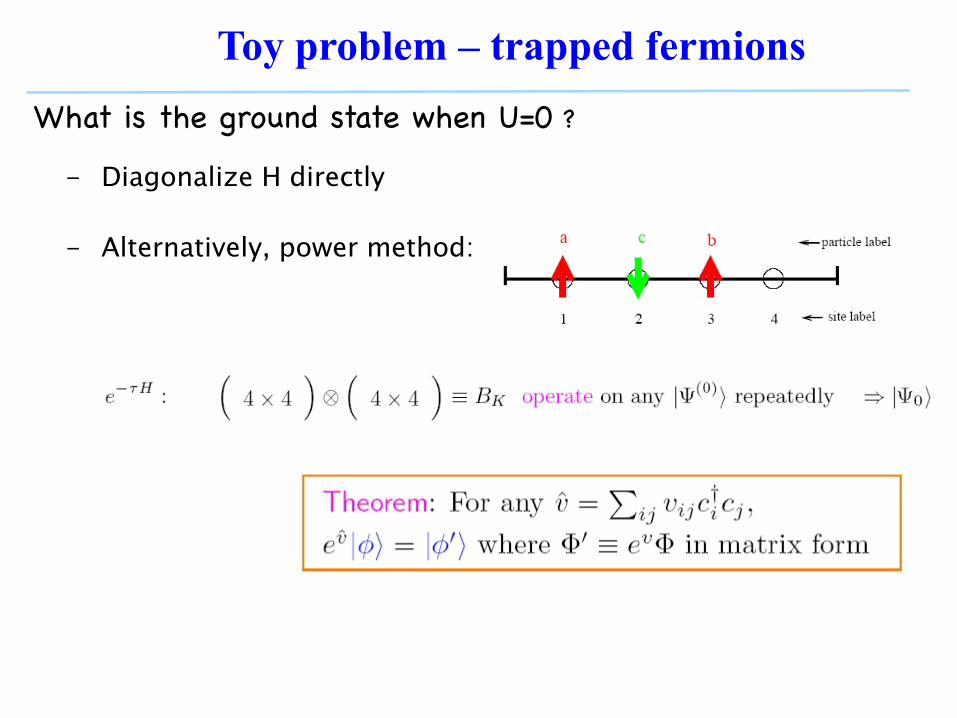
What is the ground state when U=0 ?

Toy problem – trapped fermions

- Diagonalize H directly:

Put fermions in lowest levels: many-body wf:

What is the ground state when U=0 ?

Toy problem – trapped fermions

- Diagonalize H directly

- Alternatively, power method:

To obtain ground state, use projection in imaginary-time:

(3) We have seen the time evolution operator U(t0, t) ⌘ exp(�iH(t� t0)/h) and its matrixrepresentation in x-space, K(x0, t; x, t0), known as the propagator. Here we will study theimaginary-time evolution operator and its propagator. Methods based on these have provenvery powerful for studying many-body quantum-mechanical systems and are widely used inmany practical calculations.

Specifically, we consider the operator exp(��H) (� is real) and its matrix representationK(x0, x; �) ⌘ hx0|exp(��H)|xi for a one-dimensional system with the Hamiltonian

H =p2

2m+ V (x).

For convenience let us set h = m = 1.

1. Show thatK(x0, x; �) =

X

n

e��En�?n(x

0)�n(x),

where En is an energy eigenvalue and �n(x) is the corresponding eigenfunction. Thesum is taken over the complete set of n.

2. Show that the operator exp(��H) projects out the ground state |�0i from any initialstate that is not orthogonal to the ground state. That is, given an arbitrary | (0)i thatsatisfies h (0)|�0i 6= 0, we have

lim�!1

exp(��H)| (0)i / |�0i.

3. We consider short imaginary-time �⌧ (i.e., �⌧ is a small, positive number). Show that

K(x0, x;�⌧).=

1p2⇡�⌧

exp[�(x0 � x)2

2�⌧��⌧V (x)].

The approximately equal sign, which indicates we have dropped higher order terms in�⌧ , becomes exact in the limit of infinitesimal �⌧ . (This is why we need �⌧ to besmall for this part.) Indicate clearly where the approximation occurs in your proof.

4. Now we try to construct a method to obtain the ground-state wave function. Supposewe choose a � in (2) which is finite but large enough so that the projection gives |�0ifor practical purposes. Suppose we then choose a �⌧ = �/L with L large enoughso that the error in the approximation in (3) is small. We choose a (0)(x) which isour best guess of the ground-state wave function. Using (3), express the projection|�0i .

= C exp(��H)| (0)i in real space in terms of a path integral. (No need to evaluatethe constant C.)

1

What is the ground state when U=0 ?

Toy problem – trapped fermions

- Diagonalize H directly

- Alternatively, power method:

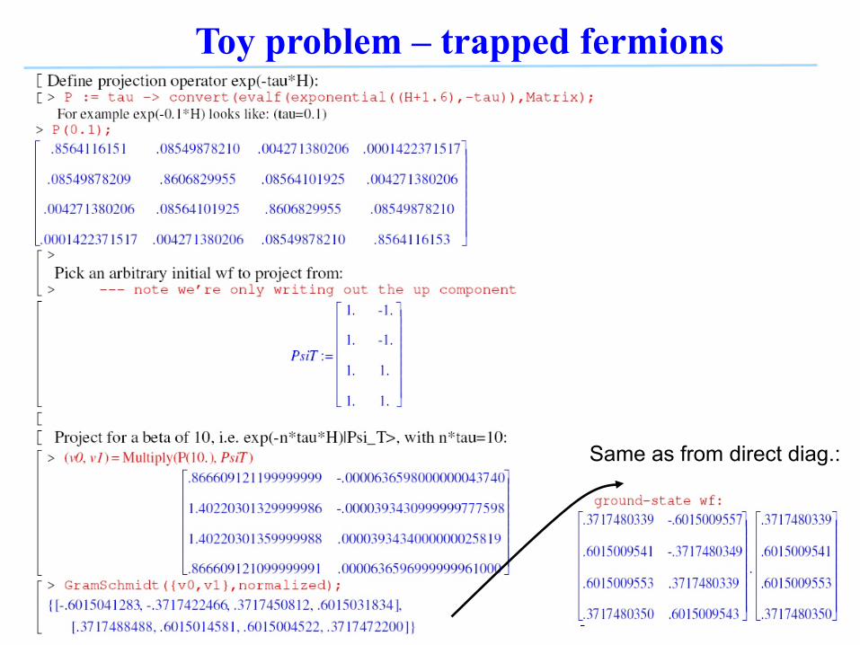
Toy problem – trapped fermions

:

Same as from direct diag.:

What is the ground state when U=0 ?

Toy problem – trapped fermions

- Diagonalize H directly

- Alternatively, power method:

• Applies to any non-interacting system

• Re-orthogonalizing the orbitals prevents fermions from

collapsing to the bosonic state

-> i.e., no ‘sign problem’ in non-interacting systems

Toy problem – trapped fermions

What is the ground state when U=0 ?

Toy problem – trapped fermions

- Diagonalize H directly

- Alternatively, power method:

What is the ground state, if we turn on U ? - Lanczos (scaling!)

- Can we still write in one-body form?

Yes, with Hubbard-Stratonivich transformation

Hubbard-stratonivich transformation

AFQMC: “emergent” mean-field solutions

Back to toy problemWhat is the ground state, if we turn on U ?

- With U, same as U=0, except for integral over x Monte Carlo

Recall: Monte Carlo methodsWe will use two things which are foundations to QMC1)Monte Carlo is great at evaluating many-dimensional

integrals (most efficient beyond d>4~6)2)Monte Carlo can solve integral equations via random walks

1) Monte Carlo integration

2) Random walks to solve integral equations:

.= e��H1e��H2 +O(�2)

e��HLDA(n(0)) |SD(0)�|SD(1)�e��HLDA(n(1))|GS�

ev2=

1��

� ⇥

�⇥e��2

e2�vd⇥

Summary: an auxiliary-field perspective

Propagation leads to multi-determinants

e��HLDA(n) .= e��H1e��Hxc(n)• Independent-electron:

e��HConsider the propagator

Thus, LDA calculation:

...Single-determinant solution

H2 = ��

�

v2�• Many-body:

Different form --> Hartree, HF, pairing, ..Importance sampling to make practical SZ & Krakauer, ’03 Purwanto & SZ, ’05

Two-site Hubbard modelAn illustration: H2 molecule:

electron,

electron,

spin

spin

Periodic box (supercell)

ion, fixed, +1 charge

tight binding/minimal basis => 1-band Hubbard model with U/t

small U/t* 1 determinant

large U/t

+

* multi determinants* correlation* note ‘antiferromagnetism’

Two-site Hubbard modelHow AFQMC works:

H2 molecule

mean-field auxiliary-field QMC

wf wf

wf

+ ....+- Formalism similar to LGT- But this formulation allows a natural way to control sign problem

Full electronic Hamiltonians• Electronic Hamiltonian: (Born-Oppenheimer)

can choose any single-particle basis

• An orbital:

• A Slater determinant:MnO

Slater determinant random walk (preliminary I)

Slater determinant random walk (preliminary II)

HS transformation:

‘density’ decomposition

derive

Slater determinant random walk (preliminary II)

HS transformation for full V-matrices (e.g. Gaussian basis sets)

modified Cholesky decomposition

can be realized with N^3 cost,

with Jmax typically 4--8*N

Vijkl.=

�Jmax�=1 L�

ij L�kl

Purwanto et al, J. Chem. Phys. 135, 164105 (2011)

Summary: AF QMC framework

H-S transformation

Schematically:

next

SZ, Carlson, GubernatisSZ, Krakauer

Exact so far (why don’t we use path-integral formalism? later)

Random walks in Slater determinant space:

e�v

Structure -- loosely coupled RWs of non-orthogonal SDs:

A step advances the SD by ‘matrix multiplications’ MnO

.

...

ψ1

ψΝ

ψ2

ψ1ψ2

ψΝ

Summary: AF QMC framework

N is size of ‘basis’

->

Gaussian, or ‘Ising’ variable

NxN matrix1-body op

.

...

ψ’1

ψ’Ν

ψ’2

ψ’1ψ’2

ψ’Ν

Importance sampling -> better efficiency

Summary: AF QMC framework

How does the weight ‘w’ come about?

We have formulated this as branching random walks

Basic idea of AFQMC, done with path-integrals over AF paths, has been around since the ‘80s. Koonin; Scalapino, Sugar, White; Hirsch; Baroni & Car; Sorella; Fahy & Hamann; Baer et. al. ....

The new formulation - allows a close connection with DFT and HF - makes possible a way to control the sign problem

� = UDV

0.5 1 1.5 2 2.5 3projection time

-16

-14

-12

-10

-8

-6

-4

E

standard

Hubbard model 4x4, n=0.875, U/t=8 (strongly corr)

Exponential noise

The sign/phase problem

- More severe at lower T, larger system size- or in the most correlated regime

Koonin; Scalapino & White et al; Baroni & Car; Fahy & Hamman; Baer et al;

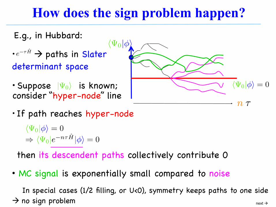
How does the sign problem happen?

• paths in Slater determinant space • Suppose is known; consider “hyper-node” line

• If path reaches hyper-node

then its descendent paths collectively contribute 0

next

E.g., in Hubbard:

• MC signal is exponentially small compared to noise

In special cases (1/2 filling, or U<0), symmetry keeps paths to one side no sign problem

Sign/phase problem is due to -- “superexchange”:

MnO

The sign problem

ψ1

ψ2

ψ1

Slater det. - antisymmetricψΝ

.

.

ψ2

ψΝ

.

.

To eliminate sign problem:��T |�⇥ = 0Use to determine if ”superexchange” has occurred

SZ, Carlson, Gubernatis, ’97; SZ ’00; Chang & SZ ’10

How to control the sign problem?

next

keep only paths that never reach the node

requireZhang, Carlson, Gubernatis, ’97Zhang, ’00

• Constrained path appr.

Trial wave function used to make detection

Connection to fixed-node, or restricted path (Ceperley), but in Slater determinant space --> different behavior

0.5 1 1.5 2 2.5 3projection time

-16

-14

-12

-10

-8

-6

-4

E

standard

0.5 1 1.5 2 2.5 3projection time

-16

-14

-12

-10

-8

-6

-4

E

standard with constraint

0.5 1 1.5 2 2.5 3projection time

-16

-14

-12

-10

-8

-6

-4

E

standard with constraintexact

4x4, n=0.875, U/t=8

Controlling the sign/phase problem

- Free-projection is exact, but exponential scaling- Constraining the paths to remove contamination - N^3 scaling, approximate -- high accuracy- Constraint release: a systematically improvable approach with more

computational cost

-12

-11.9

-11.8

-11.7

-11.6

-11.5

-11.4

-11.3

-11.2

-11.1

-0.1 0 0.1 0.2 0.3 0.4 0.5 0.6 0.7 0.8

cpmc release

EDRCMCCPMC

release

Can release constraint Shi & SZ (PRB, 2013)

constrained

~ 1/2 Trotter error @dt=0.05

(also Ceperley; Sorella)

Controlling the sign/phase problem: accuracy

0 1 2 3 4 5 6 7 8U/t

0

1

2

3

4

5

6

7

8

<V>

exactFE

0 1 2 3 4 5 6 7 8U/t

0

1

2

3

4

5

6

7

8

<V>

exactconstraint, FEFE

0 1 2 3 4 5 6 7 8U/t

0

1

2

3

4

5

6

7

8

<V>

exactconstraint, FEFEUHF

0 1 2 3 4 5 6 7 8U/t

0

1

2

3

4

5

6

7

8

<V>

exactconstraint, FEconstraint, UHFFEUHF

0 1 2 3 4 5 6 7 8U/t

0

1

2

3

4

5

6

7

8

<V>

exactreleaseconstraint, FEconstraint, UHFFEUHF

Avg interaction energy vs U

<V> = U*(double occupancy)

- Recovers from incorrect physics of constraint

- Insensitive to choices of constraining wf

4x4, n=0.875

Shi & SZ (unpublished, 2013)

Sign/phase problem is due to -- “superexchange”:

The phase problem

ψ1

ψ2

ψ1

Slater det. - antisymmetricψΝ

.

.

ψ2

ψΝ

.

.

To eliminate sign problem:��T |�⇥ = 0Use to determine if ”superexchange” has occurred

To eliminate phase problem: Generalize above with gauge transform --> “phaseless constraint’’

SZ & Krakauer, ’03; Chang & SZ, ’10

H2 = ��

�

v2�Many-body:

ev2=

1��

� ⇥

�⇥e��2

e2�vd⇥

Controlling the phase problemSketch of approximate solution:

• Modify propagator by “gauge transformation’: phase degeneracy (use trial wf)

• Project to one overall phase: break “rotational invariance”

• subtle, but key, difference from: real<ΨT|φ> 0 (Fahy & Hamann; Zhang, Carlson, Gubernatis)

After:Before:

0 2 4 6 8 10 12expt / exact (eV)

0

2

4

6

8

10

12

AF

QM

C (e

V)

0 2 4 6 8 10 12expt / exact (eV)

0

2

4

6

8

10

12

QM

C (e

V)

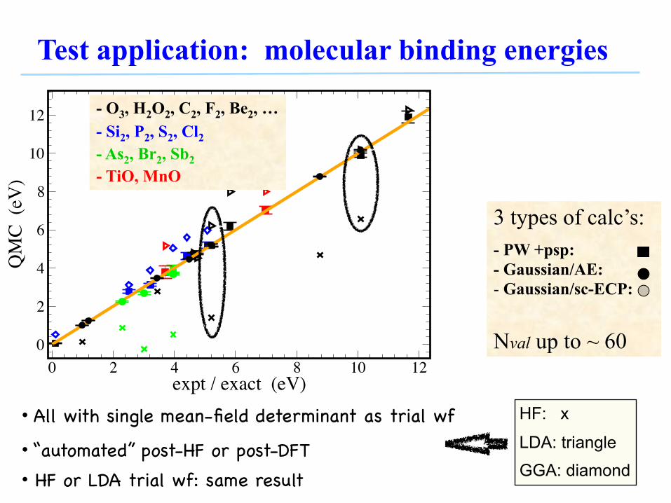
3 types of calc’s:- PW +psp: - Gaussian/AE:- Gaussian/sc-ECP:

Nval up to ~ 60

Test application: molecular binding energies

• All with single mean-field determinant as trial wf

• “automated” post-HF or post-DFT • HF or LDA trial wf: same result

- O3, H2O2, C2, F2, Be2, …- Si2, P2, S2, Cl2- As2, Br2, Sb2- TiO, MnO

HF: x

LDA: triangle

GGA: diamond

F2 bond breaking

Mimics increasing correlation effects:

Dissoc. limitEquilibrium

•CCSD(T) methods have problems (excellent at equilibrium)

•UHF unbound

•QMC/UHF recovers despite incorrect trial wf --- uniformly accurate

“bonding” “insulating”

F F

(removes spin contamination)

RCCSDTQ: Musial & Bartlett, ’05

F2 bond breaking --- larger basis

Potential energy curve:• LDA and GGA/PBE - well-depths too deep • B3LYP - well-depth excellent - “shoulder” too steep

• Compare with experiment spectroscopic cnsts:

cc-pVTZ

Purwanto et. al., JCP, ‘08

Periodic Solids Silicon structural phase transition (diamond --> -tin):

150 200 250 300 350

Volume (a0

3)

−578.09

−578.08

−578.07

−578.06

−578.05

−578.04

−578.03

−578.02

−578.01

−578.00

Ener

gy (E

h)

~15mHa

�

• transition pressure is sensitive: small dE

method P (GPa)LDA 6.7GGA (BP) 13.3GGA (PW91) 10.9GGA (PBE) ~8.9DMC (Alfe et al ’04) 16.5(5)AFQMC 12.6(3)experiment 10.3-12.5

• AFQMC✓54-atom supercells+finite-size correction✓PW + psp✓uses LDA trial wf

• Good agreement w/ experiment --- consistent w/ exact free-proj checks

Purwanto et. al., PRB, ’09

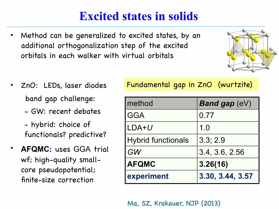
Fundamental gap in ZnO (wurtzite)

• Method can be generalized to excited states, by an additional orthogonalization step of the excited orbitals in each walker with virtual orbitals

Excited states in solids

• ZnO: LEDs, laser diodes band gap challenge:

- GW: recent debates - hybrid: choice of functionals? predictive?

• AFQMC: uses GGA trial wf; high-quality small-core pseudopotential; finite-size correction

method Band gap (eV)GGA 0.77LDA+U 1.0Hybrid functionals 3.3; 2.9GW 3.4, 3.6, 2.56AFQMC 3.26(16)experiment 3.30, 3.44, 3.57

Ma, SZ, Krakauer, NJP (2013)

�

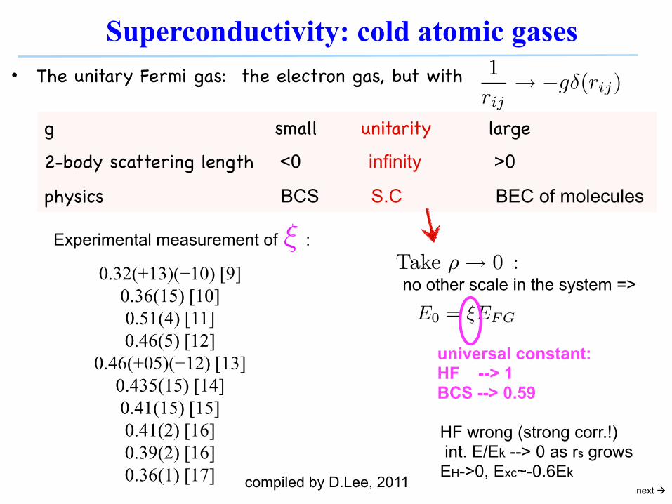
• The unitary Fermi gas: the electron gas, but with

g small unitarity large

2-body scattering length <0 infinity >0

physics BCS S.C BEC of molecules

next

1rij⇥ �g�(rij)

universal constant:HF --> 1BCS --> 0.59

Experimental measurement of :

Cold atom experimental values for

0.32(+13)(−10) [9]

0.36(15) [10]

0.51(4) [11]

0.46(5) [12]

0.46(+05)(−12) [13]

0.435(15) [14]

0.41(15) [15]

0.41(2) [16]

0.39(2) [16]

0.36(1) [17]

8  8 

references in arXiv: 1104.2102 [cond-mat-quant-gas]

compiled by D.Lee, 2011

no other scale in the system =>

E0 = �EFG

Take �� 0 :

Superconductivity: cold atomic gases

HF wrong (strong corr.!) int. E/Ek --> 0 as rs growsEH->0, Exc~-0.6Ek

• In this case, no sign problem in AFQMC. Trial wf is projected BCS (AGP)

Both can be done (Carlson, Gandolfi, Schmidt, SZ: arXiv:1107.5848)

same scaling as single Slater determinant

next

Exact result:� = 0.372(5)

4

0 0.1 0.2 0.3 0.4

!1/3

= "N1/3

/L

0.32

0.34

0.36

0.38

0.40

0.42

#

N = 38

N = 48

N = 66

$k

(4)

$k

(h)

$k

(2)

FIG. 1. (color online) The calculated ground state energyshown as the value of ⇥ versus the lattice size for variousparticle numbers and Hamiltonians.

100� reduction in computer time, compared to the usualFG importance function. The improvement increased to1500� for N = 38 in a 123 lattice. For larger systems,the discrepancy is much larger still; indeed the statisticalfluctuations from the latter are such that often meaning-ful results cannot be obtained with the run configurationsdescribed above.

In Fig. 1 we summarize our calculations of the energyas a function of ⌅1/3 where ⌅ = N/N3

k , and the particlenumber is N = 38, 48 or 66. We plot ⇥, Eq. 1, where wehave in all cases used the infinite system free-gas energy

EFG = 35�2k2

F2m with k3F = 3⇤2 N

�N3kas the reference.

Hamiltonian N ⇥ err A err

�(2)k 14 0.39 0.01 0.21 0.12

38 0.370 0.005 0.14 0.04

66 0.374 0.005 0.11 0.04

�(4)k 38 0.372 0.002

48 0.372 0.003

66 0.372 0.003

�(h)k 4 0.280 0.004 -0.28 0.05

38 0.380 0.005 -0.17 0.03

48 0.367 0.005 -0.05 0.03

66 0.375 0.005 -0.13 0.03

TABLE II. Energy extrapolations to infinite volume, zerorange limit for various particle numbers N and di�erentHamiltonians. The term linear in the e�ective range, A, isalso shown where it is not tuned to zero.

DMC calculations have found converged results whenusing 66 particles[11, 12], and our results confirm this.The di�erences between 38 and 66 particles are rathersmall. Our calculations with 14 particles show a signif-icant size dependence, and with 26 particles the e�ectsare still noticeable. These are not shown on the figure.We have also computed the energy for 4 particle systems

for a variety of lattice sizes and find agreement with Ref.[25]. The error bands in the figure provide least-squaresestimates for the one sigma error based upon quadraticfits to the finite-size e�ects. The fits are of the formE/EFG = ⇥+A⌅1/3 +B⌅2/3. For the interactions tunedto re = 0, a fit with A fixed to zero is used. Includinga linear coe⌅cient in the fit yields a value statisticallyconsistent with zero.

The extrapolation in lattice size for the k2 and Hub-bard dispersions show opposite slope as expected fromthe opposite signs of their e�ective ranges. The extrap-olation to ⌅ ⇥ 0 is consistent with ⇥ = 0.372(0.005) inall cases. Our final error contains statistical componentand the errors associated with finite population sizes andfinite time-step errors. This value is below previous ex-periments, but more compatible with recent experimentalresults of the Zwierlein group[8].

0 0.1 0.2 0.3 0.4

kF r

e

0.36

0.37

0.38

0.39

0.4

0.41

0.42

!

N = 66

N = 38 DMC

FIG. 2. (color online) The ground-state energy as a functionof kF re: comparison of DMC and AFQMC results. Dashedlines are DMC results, shifted down by a constant to enablecomparison of the slopes.

We have also examined the behavior of the energyas a function of kF re for finite e�ective ranges. It hasbeen conjectured[28] that the slope of ⇥ is universal:⇥(re) = ⇥+SkF re. Of course a finite range purely attrac-tive interaction is subject to collapse for a many-particlesystem, but a small repulsive many-body interaction orthe lattice, where double occupancy of a single species isnot allowed, is enough to stabilize the system. Our re-sults are consistent with the universality conjecture. Inparticular our results for zero e�ective range approachthe continuum limit with a slope consistent with zero.

Figure 2 compares the AFQMC results for the �(2)k in-teraction with the DMC results [11, 12] for various valuesof the e�ective range. The AFQMC produces somewhatlower energies than the DMC, consistent with the upper-bound nature of the DMC calculations. For the slope S of⇥ with respect to finite re, the fit to the N = 66 AFQMCresults yields S = 0.11(.03). Similar fits to the AFQMC

data with the Hubbard dispersion �(h)k for N = 66 yield

MIT expt (Zwierlein group):

0.376(5) arXiv:1110.3309

Need ��AGP|c†i cj |�⇥ and ��AGP|c†i cj |�⇥

Superconductivity: cold atomic gases

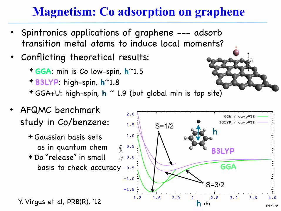
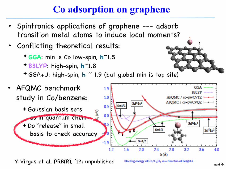
• Spintronics applications of graphene --- adsorb transition metal atoms to induce local moments?

• Conflicting theoretical results:

Magnetism: Co adsorption on graphene

next

−1.5

−1.0

−0.5

0.0

0.5

1.0

1.5

2.0

1.2 1.6 2.0 2.4 2.8 3.2 3.6 4.0

E b (eV)

h (Å)

GGA / cc−pVTZB3LYP / cc−pVTZ

h

S=3/2

S=1/2

✦ GGA: min is Co low-spin, h~1.5✦ B3LYP: high-spin, h~1.8✦ GGA+U: high-spin, h ~ 1.9 (but global min is top site)

• AFQMC benchmark study in Co/benzene:

✦ Gaussian basis sets as in quantum chem✦ Do “release” in small basis to check accuracy GGA

B3LYP

Y. Virgus et al, PRB(R), ’12

h

−1.5

−1.0

−0.5

0.0

0.5

1.0

1.5

2.0

1.2 1.6 2.0 2.4 2.8 3.2 3.6 4.0

E b (eV)

h (Å)

GGA / cc−pVTZB3LYP / cc−pVTZ

−1.5

−1.0

−0.5

0.0

0.5

1.0

1.5

2.0

1.2 1.6 2.0 2.4 2.8 3.2 3.6 4.0

E b (eV)

h (Å)

GGA / cc−pVTZB3LYP / cc−pVTZAFQMC / cc−pVTZ

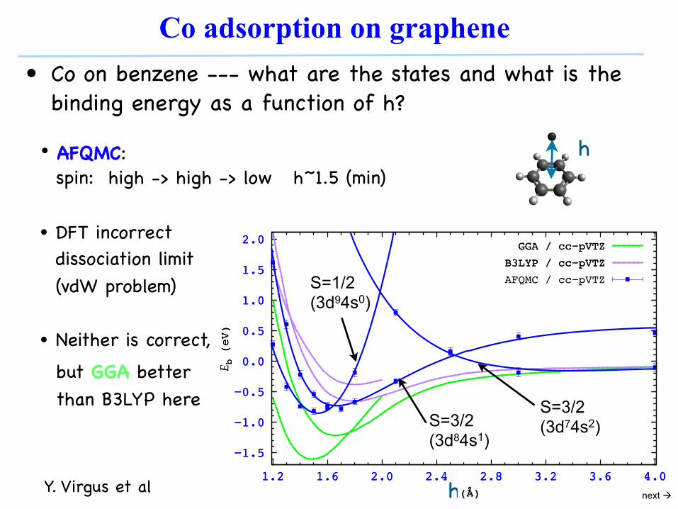
• Co on benzene --- what are the states and what is the binding energy as a function of h?

Co adsorption on graphene

next

S=3/2 (3d84s1)

• AFQMC: spin: high -> high -> low h~1.5 (min)

S=1/2 (3d94s0)

S=3/2 (3d74s2)

• DFT incorrect dissociation limit (vdW problem)

• Neither is correct, but GGA better than B3LYP here

Y. Virgus et al

h

h

• What are the states and what is the binding energy as a function of h? (STM?)

Co adsorption on graphene

next

S=3/2 (3d84s1)

✦ Embedding ONIOM correction (W/ GGA or B3LYP)

✦ Nominal spin: high -> high -> low h~1.5 (min)

S=1/2 (3d94s0)

S=3/2 (3d74s2)−0.3

0.0

0.3

0.6

0.9

1.2

1.2 1.6 2.0 2.4 2.8 3.2 3.6 4.0

E b (

eV)

h (Å)

AFQMC / cc−pwCVTZAFQMC / cc−pwCVQZ

AFQMC / CBS

Y. Virgus et al, PRB(R) ’12

✦ double well feature

✦ comparable binding energies, small barrier

• Spintronics applications of graphene --- adsorb transition metal atoms to induce local moments?

• Conflicting theoretical results:

Co adsorption on graphene

next

✦ GGA: min is Co low-spin, h~1.5✦ B3LYP: high-spin, h~1.8✦ GGA+U: high-spin, h ~ 1.9 (but global min is top site)

• AFQMC benchmark study in Co/benzene:

✦ Gaussian basis sets as in quantum chem✦ Do “release” in small basis to check accuracy

Y. Virgus et al, PRB(R), ’12; unpublished

• Model for CuO plane in cuprates? • Half-filling: antiferromagnetic (AF) order (Furukawa & Imada 1991; Tang & Hirsch 1983; White et al, 1989; .…)

Magnetic properties in the 2D Hubbard model

AF correlation:

next

12 x 12, n = 1.0, U/t=4

What happens to the AF order upon doping?

• Use rectangular lattices to probe correlation length L > 16

• Up to 8x128 supercell (dimension of CI space: 10^600 !)

• Detect spatial structures using correlation functions

Spin-spin correlation

8x32

n = 0.9375

8x64

8x32

8x64

! Periodic boundary condition is used when calculating C(r)

! The observed structure emerges from a free electron trial state

“staggered”: (-1)^y C(x,y)

Wednesday, May 11, 2011

AFM? Phase separation? Stripes? Large body of numerical work --- Conflicting results

Challenges: - Many competing orders with tiny energy differences: high accuracy - Reaching the thermodynamic limit reliably sensitivity to both finite-size and shell effects (numerical derivative!)

- GFMC (Cosentiri et al.; Sorella et al.)- GFMC in t-J (Hellberg & Manousakis, 1997, 2000)- DMRG w/ open BC (White, ...)

- DMFT (Zitler et al. 2002)

- DCA (Macridin, Jarrell et al. 2006)- Variational Cluster (Aichhorn et al. 2007)- many others ….

Challenges for many-body calculations

Furukawa and Imada, 1992

(13,13)

(25,25)

57

0.0 0.2 0.4 0.6 0.8 1.0n

-1.5

-1.0

-0.5

0.0

e(n)

8x8

U=2t

U=4t

U=6t

U=8t

U=00.0 0.2 0.4 0.6 0.8 1.0n

-1.5

-1.0

-0.5

0.0

e(n)

8x812x12

0.0 0.2 0.4 0.6 0.8 1.0n

-1.5

-1.0

-0.5

0.0

e(n)

8x812x1216x16

0.0 0.2 0.4 0.6 0.8 1.0n

-1.5

-1.0

-0.5

0.0

e(n)

8x8

frustrated long wavelength mode ? phase separation ?

n ⇠ 0.92

n = 1

�2e(n)

�n2< 0

Equation of state -- 2D Hubbard model

0.8750 0.9375 1.0000n-0.002

0.000

0.002

ε(n)-εM(n)

8x8

• Free-electron trial w.f.• Twisted average boundary condition (Zhong & Ceperley, ’01)

20 ~ 300 random twists• Different lattice sizes

in good agreementfor n < 0.9

• “Unstable” region is foundon 8x8, 12x12, 16x16

• Use rectangular lattices to probe correlation length L > 16• Up to 8x128 supercell (dimension of CI space: 10^600 ! vs. ‘DFT’ 1k x 1k)• Detect spatial structures using correlation functions

Spin-spin correlation

8x32n = 0.9375

8x64

8x32

8x64

Periodic boundary condition is used when calculating C(r)

The observed structure emerges from a free electron trial state

“staggered”: (-1)^y C(x,y)

• TABC removes one-body shell effects, but not two-body finite-size effects:

59

0.8750 0.9375 1.0000n-0.002

0.000

0.002

ε(n)-εM(n)

8x8

Maxwell construction

0.00 0.02 0.04 0.06 0.08 0.10 0.12 0.141 / Ly

-0.949

-0.948

-0.947

-0.946

-0.945

-0.944

-0.943

ε

8x8

8x128x16

8x328x64

0.00 0.02 0.04 0.06 0.08 0.10 0.12 0.141 / Ly

-0.949

-0.948

-0.947

-0.946

-0.945

-0.944

-0.943

ε

8x8

8x12

0.00 0.02 0.04 0.06 0.08 0.10 0.12 0.141 / Ly

-0.949

-0.948

-0.947

-0.946

-0.945

-0.944

-0.943

ε

8x8

8x128x16

8x328x64

0.00 0.02 0.04 0.06 0.08 0.10 0.12 0.141 / Ly

-0.949

-0.948

-0.947

-0.946

-0.945

-0.944

-0.943

ε

8x8

8x128x16

8x328x64

0.00 0.02 0.04 0.06 0.08 0.10 0.12 0.141 / Ly

-0.949

-0.948

-0.947

-0.946

-0.945

-0.944

-0.943

ε

8x8

8x128x16

8x328x64

0.00 0.02 0.04 0.06 0.08 0.10 0.12 0.141 / Ly

-0.949

-0.948

-0.947

-0.946

-0.945

-0.944

-0.943

ε

8x8

8x128x16

8x328x64

• Instability is from frustration of SDW due to finite size• At n = 0.9375, need L>~32 to detect SDW state (Previous calculations: Ly~12, with large shell effects)

Rectangular supercells, increasing Ly

Equation of state, again

Doping h = (1-n) dependence

• Wavelength decreases with doping; as does the amplitude• SDW terminates at finite doping (~0.15), enters paramagnetic state• Wavelength appears

Wavelength versus doping

4x64,  U/t =  4.0

� 1/hC.-C. Chang & SZ, PRL,’10

• At U/t=4, charge is uniform: - No peak in charge struc. factor - holes fluid-like (de-localized)

• At U/t=8-12, CDW develops: - Peak in structure factor- Clumps of density=1, separated by

dips (SDW nodes)- Consistent with DMRG results at

large U/t (White et al, ’03, ’05)- holes Wigner-like (localized)

Dependence on U

S�(k)

�(r)

Smectic state - connection and difference to ‘stripe phase’:

• Computational framework for correlated electronic systems (equilibrium)✦ Both materials specific and model Hamiltonians✦ Much development still to be done, but a blueprint for systematic calculations

• Exact calculation of Bertch parameter in BCS-BEC crossover • Co adsorption on graphene: double-well high-low spin states

• Quantum simulations provide a ‘new’ tool for studying quantum matter: ✦ The algorithms have reached a turning point ✦ Need you! Many opportunities for breakthroughs

Summary

• Magnetic phases in 2D Hubbard:

✦ AF SDW, long wavelength modulation✦ Wavelength ✦ SDW amplitude decreases with doping, vanishes at n~0.85(5)✦ Holes “liquid like”

� 1/h