pose is to find the exact sequence of road segments that thestolen property is driven through so as to pinpoint its finaldestination. The reconstruction of the path consists of twostages — 1) estimation of turns and distances between suc-cessive stops and/or turns, and 2) application of Viterbi de-coding and a Hidden Markov Model (HMM) on the streetmap to identify the path from distance and turn estimates. Inthis section, we describe the process of obtaining turn anddistance estimates and discuss the path reconstruction pro-cess in Section 6.

Any rigid body’s spatial movement in space can be de-scribed with the help of six parameters: namely three trans-latory (x-, y-, z-acceleration) and three rotatory components(x-, y-, z-angular velocity). As described earlier, the tag nodeused in the AutoWitness system is equipped with a 3 axisaccelerometer coupled with a 3 axis gyroscope. The threeacceleration sensors and three gyros have been put togetherin such a way that they form an orthogonal system. The ac-celerometer has a 3-dimensional Cartesian frame of refer-ence with respect to itself, represented by the orthogonal x,y, and z axes. In addition, we define a cartesian frame of ref-erence with respect to the vehicle that the tag node is in. Thevehicle’s frame of reference is represented by the orthogonalX, Y, and Z axes, with X pointing directly to the front, Y tothe right, and Z into the ground. If the tag node’s coordi-nate system was perfectly aligned with that of the car’s, andthe obtained signal from the tag was continuous, integratingthe individual translatory and rotatory components recordedon the accelerometers and gyros respectively would tell usthe exact position and attitude of the burglar’s car. For astraight road segment, a double integration of the accelera-tion data would yield the distance traveled from the startingpoint and since the gyros provide output data representingrotation speed (not angular acceleration), a single integra-tion of the gyro signal would yield the total change in theattitude of the burglar’s car. Performing these calculationsperiodically would enable the ideal system to trace the car’smovement with respect to a (virtual) reference point and toindicate its speed, current position and heading. However,the assumption of perfect alignment is unrealistic and in mostcases when a theft occurs the stolen object will be placed in atilted configuration resulting in an arbitrary disorientation ofthe axis of accelerometers with respect to the car’s coordinatesystem. Integrating readings from a disoriented accelerom-eter results in huge estimation errors for both distance andangles. Additionally, the measurements obtained from lowcost inertial sensors are quite noisy and suffer from largedrifts. In Section 5.1, we present our method of obtainingangle estimates from the gyroscope measurements, in Sec-tion 5.2 we describe the process of reorienting the axes ofaccelerometers every time there is a change in its orientationwith respect to the vehicle, and in Section 5.3, we describeour approach of estimating the distance traveled betweensuccessive stops and/or turns from accelerometer and gyro-scope measurements. The stops are detected using a similardecision-tree based classifier as the one used for detectingvehicular movement (see Section 4.1).

(a) Lane Change followed by aright turn

(b) Corresponding yaw mea-surements

(c) First difference in yaw (d) Estimation of angles

Figure 6. Gyroscope measurements during turns andlane changes

5.1 Obtaining Angle EstimatesWe use the gyroscopes and accelerometers to estimate the

angle of change in the direction of movement of the vehicle.In strapdown inertial navigation applications, gyroscopes areused to estimate instantaneous attitude of the object along afixed reference frame, by a single integration of the angularvelocity. The instantaneous attitude along each axis (X,Y,Z)can be represented using Direction Cosine matrix, Euler An-gles or Quaternions. We use Euler Angle system to maintainthe instantaneous attitude information. Rate-grade low-costgyroscopes generally suffer from two kinds of errors — scalefactor error and static bias [13]. The scale factor error thatmay be introduced due to mounting and placement errorswhen putting the gyroscopes on the board, can be estimatedonce for each board using a turn table.

Static bias is the output produced by gyroscope whenthere is no angular velocity applied to it. This value is of-ten not a constant, and when integrated to find the angle ofrotation may lead to large drifts over time. We account forthis potential error by estimating the drift at every stop.

Although we are interested in measuring the change inthe angle of heading of the vehicle (for use in map match-ing), the tag may experience a change in orientation not onlydue to legitimate turns and curves in the road, but also dueto change in its orientation from the vehicle’s frame of ref-erence (e.g. due to jerks, or skidding when taking a turn).We use the absolute value of the first difference in yaw read-ings to detect these changes in orientation. We maintain twothresholds (Dh ≥ Dl) for amplitude so as to detect a spikein the first difference feature (when it rises above Dh) andwe record the time it takes for the first difference to returnto normal (when it drops below Dl). This duration is calledthe activation time. Figure 6 shows the effect of lane shiftsand turns on these two features. Gyroscope measurements

Figure 7. Illustration of various steps to reduce ac-celerometer noise. First the raw signals are passedthrough a 2nd order butter worth filter, then the median iscomputed over a window of 20 samples, finally the meanis calculated over 10 medians. .

captured during the activation time are used for computingthe change in angle of the tag. The axes of the accelerom-eter are reoriented to the vehicle’s frame of reference usingthe reorientation module any time the gyroscope indicates achange in orientation (see Section 5.2). The change in theorientation of accelerometer computed by the reorientationmodule (which represents the change in the tag’s orientationfrom vehicle’s frame of reference) is then accounted for inthe angle of turn computed from gyroscope measurements toobtain the change in angle of the vehicle.5.2 Reorientation of Accelerometer Axes

To measure acceleration in the forward direction, thedominant (virtual) axis of the accelerometer (which need notbe aligned with any of the designated axes) needs to be de-termined so that the acceleration values used are indicativeof actual distance traveled. Since the tagged object can beplaced in any orientation, we need to find the (virtual) axisof motion. To determine the dominant axis, we use the ap-proach proposed in [21]. In addition, the orientation of thetag may change en-route due to movement of the asset thathouses the tag. We recompute the dominant axis anytime thegyroscope measurements indicate a potential change in theangle of the tag (see Section 5.1). We then use the directioncosine matrix to resolve the accelerometer readings to obtainthe acceleration in the direction of motion [29].5.3 Estimating Distance Traveled from Iner-

tial SensorsBefore the accelerometer values obtained in the direction

of motion can be used to compute distance traveled, it mustbe corrected for several potential errors. First, to removejitters and noise from the accelerometers one can either per-form a 2nd order Runge Kutta Integration [33] or pass thesignal through a 2nd order Butterworth Filter [19, 29]. Wetried out both and found that the later worked for us better.Due to the high sampling rate of our accelerometers (200 Hz)and jerks experienced on the road the obtained signals still

suffered from high amplitude variation. Hence, they werefurther smoothed by taking a median of 20 samples and thentaking the mean of 10 such obtained medians. This proce-dure yielded only a single acceleration value for each 1 sec-ond interval, representing the average acceleration of drivingduring that second.

Second, urban streets often contain curved roads throughneighborhoods, ramp to interstates or loops. As shown inFigure 8 when a car drives through a curved road even forsmall speeds the centrifugal force can be substantial and thereadings from the accelerometers is actually a representationof the tangential acceleration generated by the car. If the un-transformed signal is integrated to find the distance traveledon the curved segment it results in significant drift. The truecomponent of motion along the road is given by the resul-tant of the two opposing forces namely the tangential forceand the centripetal force (or the force generated by the steer-ing wheels to stay inside curve and the centrifugal force) andin order to find the actual distance traveled on the road seg-ment one needs to extract the true acceleration componentfrom the raw signal. This can be achieved with the help ofGyroscopes. While moving into a curved segment from aanother road segment the total change in yaw angle givesus the angular rotation. The angular rotation can be then beused to find the component of centripetal force which whensubtracted from the raw signals gives us the component ofacceleration along the curve. Other similar scenarios includelane changes and traveling over a hilly region or undulatedterrain as shown in Figure 8. For details, we refer the readerto Chapter 11 in [29].

Third, when an object moves from one stop to the nextstop, such as when accelerating from rest at a traffic light tocoming back to rest at the next red signal, the average ac-celeration over the interval is zero. But during transit, theaccelerometers produce highly oscilating values. In order toeliminate the drift from the measurements, we subtract themean acceleration (between two successive stops) from allrecorded acceleration values [12]. The typical speed limit

Figure 8. Accounting for radial acceleration in differ-ent scenarios: While traveling through ramps, undulatedterrain and making lane changes the true component ofthe acceleration is extracted from the raw accelerometersignals with the help of change in attitude informationfrom the Gyroscopes. This significantly reduces errors indistance approximation

35

Figure 9. Various stages in estimating the distance trav-eled between successive turns and/or stops from inertialsensors (broken lines indicate inputs).

of a vehicle in urban scenario lies below 75 mph which isvery small compared to the rotation speed of the earth’s sur-face, hence in our distance estimate computation we ignorethe Coriolis Effect produced by the earth. Figure 7 showshow the raw signal from the accelerometers are successivelyfiltered to produce good distance estimates.5.4 Implementation of Distance/Turn Compu-

tationsFigure 9 shows the overall procedure for obtaining dis-

tance estimates between successive stops. The accelerationvalue in the direction of motion is corrected for any radialacceleration. The Butterworth filter is applied next to filterout noise. The one second means computed from these mea-surements (see Section 5.3) are buffered until the next stop,at which time the bias is removed from them to derive theacceleration that can be used for distance computation. Eachsuch buffer corresponds to measurements recorded betweensuccessive stops.

The gyroscope measurements that may correspond toturns are also buffered until the next stop, at which time biascan be removed from them. Also, the buffer of accelerome-ter measurements is marked each time a potential change inorientation is suspected from gyroscope measurements. Fur-ther, the changes in orientation determined by the reorienta-tion module is also stored. At each stop, the angles for eachmarked turn is computed (see Section 5.1). The accelerome-ter buffer is then partitioned to derive the segments betweeneach successive turn. Double integration is now applied toobtain distance between each successive turns and/or stops.Both the accelerometer and gyroscope buffers are flushed outto allow for fresh recording until the next stop.6 Path Reconstruction From Distance and

Turn EstimatesOnce a sequence of turns and distance traveled between

successive turns and/or stops has been obtained, the nextchallenge is to search a map of streets to identify the se-

quence of road segments that is most likely to result into theobserved sequence of distances and turns. The problem is es-pecially challenging because 1) the initial location may notbe known deterministically due to the delay in activating thetracking module after theft is established by the theft clas-sification module (of the order of 10 seconds, which maytranslate to 100 meters), 2) the estimates of distances ob-tained from accelerometer and gyroscope readings could beoff from their actual values by up to 12%, 3) several roadsegments have similar lengths, and 4) the destination loca-tion (obtained from cell-towers) may have an uncertainty ofthe order of 100 meters.

Viterbi Decoding over Hidden Markov Model (HMM) hastraditionally been used for mapping noisy GPS measure-ments to a route [28] because a route can be considered asa sequence of road segments and the adjacency among ad-joining road segments can be used to constrain the transitionamong states (i.e., road segments). Therefore, even thoughwe do not have GPS coordinates to map to a sequence of roadsegments (contrary to most existing work on map matching),the formulation of an HMM continues to be a suitable choicedue to its ability to leverage adjacency among road segmentsto account for the uncertainty in measurements.

An HMM is a Markov process comprising of a set of hid-den states and a set of observables. Every state may emitan observable with a known conditional probability distri-bution called the emission probability distribution. Transi-tions among the hidden states are governed by a differentset of probabilities called transition probabilities. Upon ex-ecuting on a sequence of hidden states, an HMM producesa sequence of observables as its output. While the output(i.e., the list of observables) can be observed directly, thesequence of hidden states that were traversed in producingthe observed output is unknown; the problem is to determinethe most likely sequence of states that may have producedthe observed output. Viterbi decoding [31] is a dynamicprogramming technique to find the maximum likelihood se-quence of hidden states given a set of observables, emissionprobability distribution, and transition probabilities.

For map matching, hidden states usually correspond toroad segments (portion of road between two points of inter-est, which could be intersections, not necessarily neighbor-ing). The choice of observables is key to the formulationof an HMM. It is the definition of observables that can aidViterbi decoding in distinguishing one road segment from allothers. So, the observables should be as unique to the roadas possible. We considered average speed, total length of thesegment, travel time, stretch of the segment (i.e., ratio of Eu-clidean distance between the two ends and the road length),among others. Some are not as unique, while others are notstable (e.g., travel time). We decided to use two features asobservables — distance between successive stops and totallength of the segment (between successive turns that indi-cate transition to the next road segment). Both features aresimple to compute from the distance measurements, and to-gether are rather unique to a road segment, if it is sufficientlylong (i.e., if it includes some stops). Although a vehicle maynot stop at all traffic lights on a road segments, the distancetraveled between successive stops at (red) traffic lights cre-

36

Figure 10. Computation of Transition probability: Theburglar’s car takes a turn on road segment j from i andtravels a distance ’d’ before turning into another roadsegment k. ’d’ is obtained using the accelerometers henceεd is the error range associated with computing ’d’. Thetwo road segments falling within error range εd allowinga turn are Road segment k =1 and k =2. Hence the roadsegment traveled on j could be either j = 1 or j = 2. OurHMM computes the transitions probabilities for j =1 andj =2 and moves onto road segment k

ates a pattern that can be (probabilistically) matched to a roadsegment (see Figure 11). The total length of the segmentcomplements it by ensuring that the the aggregate of the dis-tance between successive stops for an entire road segmentmatches with the total length of that segment.

The starting state consists of all intersections (say, n ofthem) that fall within a radius of r from the location wherethe tag node was deployed before theft. They are assigneduniform probability, i.e., 1/n.

We next define transition probabilities. A transition is ini-tiated only when a turn is indicated from the gyroscope mea-surements, in which case the distance traveled on the pre-ceding segment and the angle of turn are used to determinethe transition probability. To limit the number of states con-sidered for transition, we consider only those states that fallwithin the error distribution of the observed length and turn.The transition probability from a road segment i completedat the (t− 1)th turn to segment j completed at the t th is de-rived using Bayesian Inferencing. For a distance d traveledon road segment j before turning to another road segment k,we denote the transition probability as Pi( j | d) (for transitionfrom state i to state j) and compute it as follows:

1. If t = 1, this is the first turn observed after the detec-tion of theft. In this case, the start state is defined asdescribed earlier.

2. For t > 1, the angle of turn (γ) is computed from gyro-scope (as described in Section 5.1).

3. The distance traveled on the jth segment (d) is com-puted using the accelerometers and gyroscope (as de-scribed in Section 5.3).

Figure 11. Stoppings estimates don’t exactly coincidewith traffic lights, hence a margin of ±εd is consideredwhile pinning to traffic lights. Once a traffic light is foundwithin error range the stopping estimates are refined bypinning to the light

4. Since d and γ are estimations of the actual measure-ments, we associate error margins εd and εγ respectivelyto them.

5. For all the road segments that begin at the end of seg-ment i, and have a length between d ± εd , (which allmay be different portions of the same road1), we pruneall the road segments j, whose angle of intersectionwith some road segment k is outside the range γ± εγ.The set of remaining road segments j are the candidateset for transition and is denoted as C (see Figure 10).

6. For all road segments in C, the prior probability Pi( j) isuniform and is given by Pi( j) = 1

|C|) .

7. Pi(d | j), the evidence for Bayesian inferencing, is es-timated from experimentation. We assume it follows aGaussian distribution whose variance σ depends on howaccurately we are able to approximate distances trav-eled on road with the help of accelerometers and gyro-

scope. Hence, P(d | j) = 1σ√

2πe−(d−d j)2

/2σ2

where d j

is the actual length of road segment j ∈C from start ofroad segment i.

8. Next, we compute the marginal probability P(d) whichis given by P(d) = ∑P( j)P(d | j).

9. Finally we compute our transition probability whichis given by the conditional probability P( j | d) =P(d| j)P( j)

P(d) .We next describe the computation of emission probability,

the probability of seeing defined observables given that the

1Once state i is defined, the angle of turn observed at the (t−1)th turn determines the road whose segment may come next andthus limits the search for the next road segment on to this road.

37

system is in a specific state. These probabilities in practiceshould reflect the characteristics of a state, and is used by theViterbi algorithm to differentiate the true state that the sys-tem is in from other probable states. If the stopping estimateswere perfect, we could assign an emission probability of 1 tothe road segment whose traffic lights matched with the stop-ping distances and 0 to others. However, the estimations ofdistance obtained from accelerometers and gyroscope have amargin of error. Additionally, a vehicle may stop some dis-tance earlier than the traffic light, if there are other vehiclesin front of it. Therefore, we assume that if the distance es-timated is d, the true distance could have a range of d± εd .Let P(y|x) denote the probability of obtaining x from dis-tance estimation when the true distance is y. For |y−x|> εd ,P(y|x) = 0; otherwise, uniform over the entire domain. Wenow describe how we use P(y|x) = 1− |y−x|

y in computingthe emission probability.

Consider a road segment s. Let the number of stops en-countered be m, where the turn into this road segment is con-sidered the first stop and the turn out of this segment to an-other road segment the last stop. Let x1,2 be the observeddistance between stops 1 and 2 and y1,i the actual distance be-tween traffic lights 1 and i, where 1≤ i≤m and |y1,i−x1,2| ≤εd . Each of these lights i become a candidate for the secondstop. First consider the case when there is only one can-didate for i for each stop (see Figure 11). Then, the emis-sion probability PE = P(y1,2, . . . ,ym−1,m|x1,2, . . . ,xm−1,m) fora sequence of observed distances in a given road segment isgiven by

PE = P(y1,m|x1,m)m−1

∏i=1

P(yi,i+1|xi,i+1) (1)

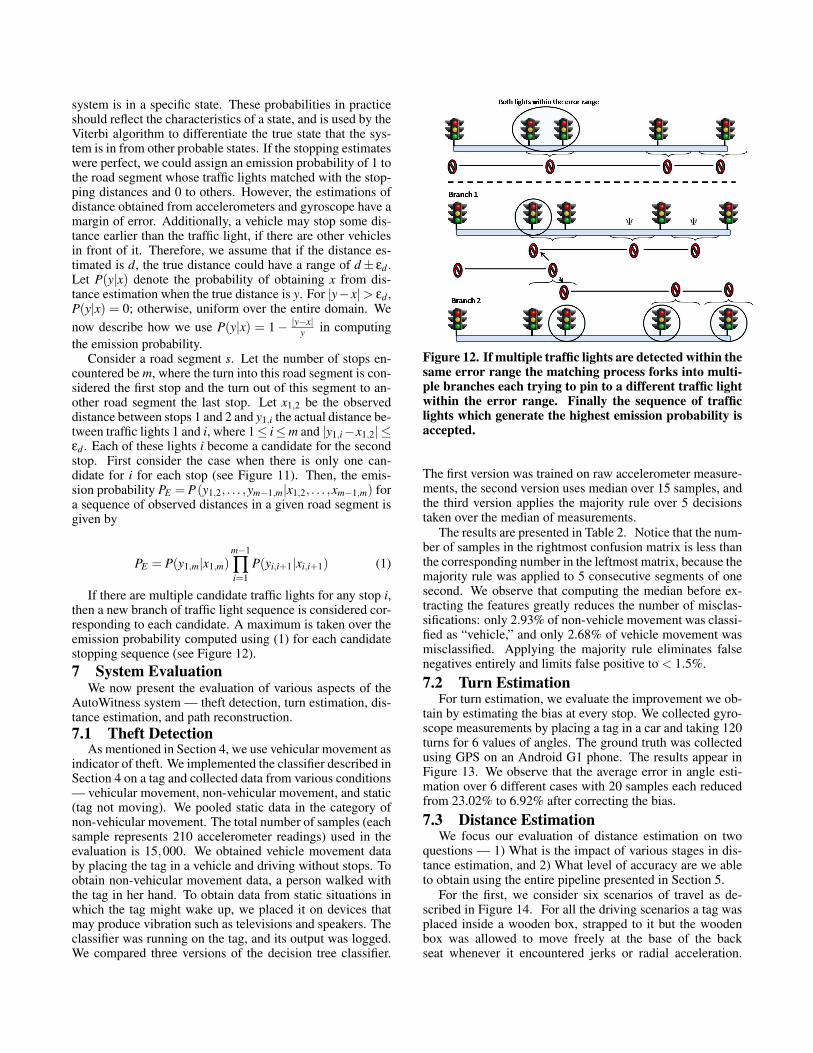
If there are multiple candidate traffic lights for any stop i,then a new branch of traffic light sequence is considered cor-responding to each candidate. A maximum is taken over theemission probability computed using (1) for each candidatestopping sequence (see Figure 12).7 System Evaluation

We now present the evaluation of various aspects of theAutoWitness system — theft detection, turn estimation, dis-tance estimation, and path reconstruction.7.1 Theft Detection

As mentioned in Section 4, we use vehicular movement asindicator of theft. We implemented the classifier described inSection 4 on a tag and collected data from various conditions— vehicular movement, non-vehicular movement, and static(tag not moving). We pooled static data in the category ofnon-vehicular movement. The total number of samples (eachsample represents 210 accelerometer readings) used in theevaluation is 15,000. We obtained vehicle movement databy placing the tag in a vehicle and driving without stops. Toobtain non-vehicular movement data, a person walked withthe tag in her hand. To obtain data from static situations inwhich the tag might wake up, we placed it on devices thatmay produce vibration such as televisions and speakers. Theclassifier was running on the tag, and its output was logged.We compared three versions of the decision tree classifier.

Figure 12. If multiple traffic lights are detected within thesame error range the matching process forks into multi-ple branches each trying to pin to a different traffic lightwithin the error range. Finally the sequence of trafficlights which generate the highest emission probability isaccepted.

The first version was trained on raw accelerometer measure-ments, the second version uses median over 15 samples, andthe third version applies the majority rule over 5 decisionstaken over the median of measurements.

The results are presented in Table 2. Notice that the num-ber of samples in the rightmost confusion matrix is less thanthe corresponding number in the leftmost matrix, because themajority rule was applied to 5 consecutive segments of onesecond. We observe that computing the median before ex-tracting the features greatly reduces the number of misclas-sifications: only 2.93% of non-vehicle movement was classi-fied as “vehicle,” and only 2.68% of vehicle movement wasmisclassified. Applying the majority rule eliminates falsenegatives entirely and limits false positive to < 1.5%.7.2 Turn Estimation

For turn estimation, we evaluate the improvement we ob-tain by estimating the bias at every stop. We collected gyro-scope measurements by placing a tag in a car and taking 120turns for 6 values of angles. The ground truth was collectedusing GPS on an Android G1 phone. The results appear inFigure 13. We observe that the average error in angle esti-mation over 6 different cases with 20 samples each reducedfrom 23.02% to 6.92% after correcting the bias.7.3 Distance Estimation

We focus our evaluation of distance estimation on twoquestions — 1) What is the impact of various stages in dis-tance estimation, and 2) What level of accuracy are we ableto obtain using the entire pipeline presented in Section 5.

For the first, we consider six scenarios of travel as de-scribed in Figure 14. For all the driving scenarios a tag wasplaced inside a wooden box, strapped to it but the woodenbox was allowed to move freely at the base of the backseat whenever it encountered jerks or radial acceleration.

38

Raw Data Median Median+MajorityVehicle Non-

Vehicle Vehicle Non-Vehicle Vehicle Non-

VehicleVehicle 4916 (98.32%) 84 (1.68%) 4866 (97.32%) 134 (2.68%) 1000 (100%) 0 (0%)Non-Vehicle 3557 (35.57%) 6443 (64.43%) 293 (2.93%) 9707 (97.07%) 29 (1.45%) 1971 (98.55%)

Table 2. Confusion matrices for the three classifiers: Using only raw measurements (left), computing median over 15samples (center), and computing median, and majority rule over 5 consecutive decisions (right). Row labels representactual values, columns represent classifier output.

This was done to simulate a real burglary incident where thewooden box represented a stolen asset. The tagged box wasdriven over 300 different road segments. We collected ac-celerometer and gyroscope measurements from the AutoW-itness tag, and ground truth using the GPS on an Android G1phone that was sampled every second. We then processedthe measurements obtained using the pipeline presented inFigure 9 on a laptop. To evaluate the impact of some of thestages in this pipeline, we omitted specific stages. In partic-ular, we evaluated the impact of reorientation, correction forradial acceleration, and correction for the drift.

The results appear in Figure 14. We observe that on roadsegments where the tag may shift its orientation due to bendsor frequent lane changes, maintaining correct orientation byreorienting the accelerometer axes can improve the error indistance estimation by over 5 times. On roads that have sig-nificant radial acceleration component due to hills or bends,correction for radial acceleration can improve the error indistance estimation by 2-3 times. Finally, correction for driftimproves the distance estimation error in all cases uniformly(by over 100%). We note that distance estimation errors alsorepresent the accuracy one would expect in locating the finaldestination, where the actual distance is the distance of thedestination from the preceding stop/turn.

For the second question, we computed the error in ourestimate of distance traveled and that obtained using GPS onthe Android G1 phone. We considered all six types of travelas described in the preceding, but spread over 300 differentroad segments whose length varied between 0.2 to 1.5 miles.We applied all stages of the distance pipeline in this case.The results appear in Figure 15. We observe that the errorsin distance estimation are usually below 10%. In some rare

Figure 13. Effect of drift due to zero offset on angle esti-mation, and angle estimation after correcting for it.

Figure 14. 1st bar denotes the actual error in distanceestimate when all stages of Figure 9 are used, 2nd bar ifreorientation is not used, 3rd bar if radial acceleration isnot accounted for, and 4th bar if the drift is not accountedfor. The conditions are — Straight road (strt), stop andgo traffic (s-go), frequent lane changes (ln-ch), frequent& rapid acceleration and deceleration) (v-sp), hilly roads(hill), and frequent (often sharp) bends (bend).

case, they reach 12.3%, but no higher.

7.4 Map ReconstructionTo evaluate the quality of path reconstruction, we focus

on three questions — 1) What is the impact of errors in dis-tance estimation in the quality of path reconstruction, 2) Howdoes the quality of path reconstruction degrade if no stops areused (i.e., only total distance of each segment is used as anobservable), 3) How does the quality of path reconstructionimprove if crude localization from cell towers is available

Figure 15. Cumulative distribution of distance approx-imation errors for 300 segments ranging from .2 to 1.5miles.

39

Figure 16. Probability of obtaining the correct path us-ing Viterbi decoding, when distance between successivestops and/or stops are used together with total length ofpath segment are used for observables, destination loca-tion is known with 100m uncertainty, and initial locationis known with 500m uncertainty. The x-axis denotes theerror in distance estimation.

at each turn, 4) How does the quality of path reconstructiondegrade if travel includes highways where long stretches oftravel can occur without any stops, and 5) How often is thetrue path in top-k paths, in cases when the true path maynot be the one found by Viterbi decoding. The last questionis relevant because in case the stolen property is not foundin the most probable destination, additional searches can bemade at other probable destination to recover it.

We use the map representation of Memphis (in Ten-nessee) from the Open Street Map project [5], which pro-vides a readily available, quite comprehensive representa-tion of the road networks of cities that can be easily pro-cessed into a data structure suitable for our Hidden MarkovModel. The Open Street Map data, which is retrievable fromthe Open Street Map website as an XML format OSM file(as well as through a web based API), consists primarily oftwo types of XML tags: Node element tags, each with aunique reference number, geographic coordinates, and metadata such as indications of traffic lights or stop signs; andWay element tags, each with sequentially ordered referencesto Node elements, as well as other meta data, such as streetname and type (highway, residential, etc.) The Node ele-ments act as ”shape points” with fixed locations, while theWay elements represent roads and paths by ”tracing along”the series of referenced Nodes in sequence.

To build a graph of the road network, we first parse theOSM file for all of the Node tags to create RoadNode ob-jects holding the location coordinates and original referencenumbers, as well as booleans to indicate if the Node is a traf-fic light, stop sign, or any other kind of potential stop. Wethen parse the file for all of the road-type Way elements (ig-noring bike trails, foot paths, and so forth) and process eachone into a series of several RoadSection objects, which rep-resent the small section of road between two Node points.Each sequential pair of Nodes (in each Way’s ordered seriesof Nodes) becomes the two end points of the RoadSection,and their latitude and longitude coordinates are used to de-termine the distance of the RoadSection via the Haversineformula, which provides great-circle distances between two

Figure 17. Similar setup as in Figure 16, but now celltower localization is available at each turn.

points on a sphere from their longitudes and latitudes. Theactual street name is stored in each RoadSection object sothat it is easily identifiable. We also compute the bearing,or angle from true North, of each road section using its twocoordinates, which is used to determine the angle betweenadjacent RoadSections. After all of the RoadSection objectsare created from the data set, we run an algorithm to popu-late each one with a list of references to other RoadSectionobjects which are adjacent to itself and the angles betweenthem and itself. The outcome of this is the graph-like datastructure with most of the details our HMM model needs.

The observables for our HMM consists of a sequence ofdistances and turns. The distances consists of either stoppingestimates between different intersections where the vehicleexperiences a red light or STOP sign or distance traveledbetween two successive turns into different road segments.Hence, in order to create the observables, we generate a syn-thetic path using the processed data from the Open StreetMap GIS database. We begin at some node in the map struc-ture and traverse through a path of road sections, recordingthe length of each section and the angles between successivesections. If the node joining two successive sections is a po-tential stop, meaning it represents a traffic light, it is chosento be marked as a stop depending on a Markov chain. TheMarkov chain represents transitions of traffic lights from redto green and vice versa. We drove across 300 traffic lightsand came up with the estimates for the transition probabil-ities for Markov chain. As per our estimate the probabilityof getting a red light, if the previous traffic light was green

Figure 18. Similar setup as in Figure 16, but distancebetween stops are not used for observables.

40

Figure 19. Similar setup as in Fig-ure 16, but highways are allowed tobe in the path.

Figure 20. Cumulative probability ofobtaining the correct path in top k-weighted paths in the case consideredin Figure 19.

Figure 21. Similar setup as in Fig-ure 19, but now cell tower localiza-tion is available at each turn.

is 0.43, and the probability of getting a red light if the pre-vious light was red is 0.55. The first light was assumed tobe Red and the next traffic light was chosen to be a stop orpass depending on the resulting state of the Markov chain.Stop signals encountered along the synthetic path were al-ways treated as STOPS.

For the turns, we used the GPS coordinates to computethe angle between two road sections. If the angle betweentwo successive sections is less than (some threshold) and thenode joining them is not marked as a stop, their distances aresummed and the next section is then considered in the samefashion. The result is a series of ground truth distances, withstops and turns in between — the output we would expectto see from our tag node. After the paths are created, ran-dom, bounded adjustments were made to the distance valuesof each road segment between successive stops and/or turnsto simulate errors in distance estimations. Since there couldbe delay of few seconds in activating the tracking module af-ter detection of theft, we generate an initial uncertainty in theoriginal location of the stolen object. We take a 500m radiusacross the original location of the stolen object and considerall intersections within the radius as a possible starting seg-ment. Additionally in all our simulations we assume that arough estimate of the final destination of the stolen object isavailable to us by virtue of cell tower localization (with anuncertainty of 100m, given the urban setting).

To observe the trend of degradation in the quality of pathreconstruction as a function of total length of the path, weconsidered a range of values for total distance of the path— 2, 5, 10, 15, 20, and 25 miles. For each value of thetotal path length, we randomly selected a starting location100 times, and for each instance, we considered 10 differentdirections for the final destination, making for 1,000 repeti-tions for each value of the path length.

For urban streets, we present the results in Figure 16. Weobserve that for path lengths ≥ 5 miles, we are able to ob-tain the true path using Viterbi decoding in > 90% cases.We also observe that the quality of path reconstruction de-grades slowly until about 20% error. Given that the errorsin distance estimation obtained from the AutoWitness tag is10% or lower in most cases, we find the quality of path re-construction promising for our application. In Figure 17 we

present the same results if crude localization is available ateach turn. We observe that with this additional information,the probability of finding the correct path is more than 99%even with 10% error in distance estimation.

Figure 18 presents the accuracy of path reconstruction ifcell tower localization at each turn is unavailable and the dis-tance between stops are not used as observables. We ob-serve that the quality of path reconstruction degrades quitea bit, but is still over 75% for total path length of 10 milesor higher. This case provides a lower bound on the perfor-mance of AutoWitness in the sense that if distance betweensuccessive stops are collapsed together (say, to tolerate stopsin the middle of the road, not at the traffic lights), the qual-ity of path reconstruction may degrade but will not be worsethan the case where distance between stops are never used.

We next consider the scenario when highways are in-cluded in the path. Figure 19 shows the probability of find-ing the correct path if cell tower localization is available onlyfor the final destination. We observe that the quality of pathreconstruction is still over 75%. Next, if we consider topk paths rather than the most probable path, then the proba-bility of finding the correct path (and the final destination)improves to over 90% if top 4 paths are considered, even fortotal path length of 5 miles (see Figure 20). Finally, we con-sider the case when cell-tower based localization is availableat each turn for the highway case. As we can see in Fig-ure 21, the quality of path reconstruction is over 90% for allpath lengths, even with 20% error in distance estimation.

8 Conclusions and Future WorkThis paper presents the design and evaluation of the Au-

toWitness system to deter, detect, and track personal prop-erty theft, improve historically dismal stolen property re-covery rates, and disrupt stolen property distribution net-works. It shows that a low-cost tag can autonomously de-tects theft while consuming ultra-low energy until stolen. Italso demonstrates the feasibility of post-facto reconstructionof the traveled path using self-contained low-cost inertialsensors on real-life city street maps. Once adopted widely,AutoWitness promises to significantly curtail property theftsthat account for over $10 billion in yearly losses and life-long traumatic experience for its victims. In addition, data

41

collected in real-life thefts could be statistically analyzed toprovide new knowledge on the behavioral pattern of suspectswhen stealing properties.

Several additional work can further improve the utility ofthe AutoWitness system. For example, dead reckoning [15]can be used to estimate the final location of the tag at its des-tination. One could obtain the distance traveled on foot sincebeing taken off the vehicle, stairs climbed, etc., to eventu-ally pinpoint the room level location in the hideout building,apartment complex, or warehouse.

AcknowledgementsThis work was supported in part by NSF grant CNS-

0721983 and Fedex Institute of Technology (FIT) at theUniversity of Memphis. The views expressed are those ofthe authors and do not necessarily reflect the views of thesponsors. We thank anonymous referees for their thought-ful comments that helped improve the quality of work pre-sented here. We would also like to thank Deputy DirectorDerek Myers (University of Memphis Police Department)and Colonel Jim Harvey (Memphis Police Department) fortheir help with providing application scenarios. Finally, wewould like to thank Mani Srivastava from UCLA, and Pra-sun Sinha and Emre Ertin from the Ohio State University forproviding valuable feedback on the overall design at earlystages of this work.

9 References[1] Brickhouse security gps tracking system. http:

//www.brickhousesecurity.com/gps-tracking-system.html.

[2] Live View GPS Asset Tracker. http://www.liveviewgps.com/all+gps+tracking+products.html.

[3] LoJack Security System for Stolen Vehicle Recovery.http://www.lojack.com/car/Pages/car-works.aspx.

[4] MobileWatch: SIM Tri Band with 1.3 Inch TFT Touch Screen +MP3/MP4 Function + 1.3 Mega Pixel Digital Camera + Bluetooth +USB port support.http://www.gizmograbber.com/ProductDetail.asp?ID=385.

[5] Open Street Map. http://www.openstreetmap.org.

[6] S Blade Antenna. http://www.rfdesign.co.za/files/5645456/Download-Library/Embedded-Antenna-Design/S-Blade-Quad-FSB35047.pdf.

[7] Telit Ge865. http://www.telit.com/en/products/gsm-gprs.php?p_ac=show&p=47.

[8] Weka. http://www.cs.waikato.ac.nz/ml/weka/.

[9] Analog Devices Inc.,Santa Clara,CA, ADXL330 Datasheet. 2005.

[10] E. Abbott, D. Powell, A. Signal, and W. Redmond. Land-vehiclenavigation using GPS. Proceedings of the IEEE, 87(1):145–162,1999.

[11] A. Benbasat and J. Paradiso. A framework for the automatedgeneration of power-efficient classifiers for embedded sensor nodes.In Proceedings of the 5th international conference on Embeddednetworked sensor systems, page 232. ACM, 2007.

[12] D. Boore. Analog-to-digital conversion as a source of drifts indisplacements derived from digital recordings of ground acceleration.Bulletin of the Seismological Society of America, 93(5):2017, 2003.

[13] J. Borenstein. Experimental evaluation of a fiber optics gyroscope forimproving dead-reckoning accuracy in mobile robots. Ann Arbor,1001:48109.

[14] S. C. (CNN). ’hillside burglar’ suspect held; l.a.’s rich relieved.Website, 2009. http://edition.cnn.com/2009/CRIME/01/23/burglary.hillside/index.html#cnnSTCText.

[15] I. Constandache, R. Choudhury, and I. Rhee. Towards mobile phonelocalization without war-driving. 2010 Proceedings IEEEINFOCOM, pages 1–9, 2010.

[16] M. Dooge and M. Walsh. Design of a track map based dataacquisition system for the dartmouth formula racing team. iMEMSTechnologies/Applications,Analog Devices, 1998.

[17] P. Dutta, J. Taneja, J. Jeong, X. Jiang, and D. Culler. A building blockapproach to sensornet systems. In SenSys ’08, pages 267–280, 2008.

[18] Q. Ladetto. On foot navigation: continuous step calibration usingboth complementary recursive prediction and adaptive Kalmanfiltering. In ION GPS, volume 2000, 2000.

[19] A. Lawrence. Modern inertial technology: navigation, guidance, andcontrol. Springer Verlag, 1998.

[20] C. Lemaire and B. Sulouff. Surface Micromachined Sensors forVehicle Navigation Systems. Advanced microsystems for automotiveapplications 98, page 103, 1998.

[21] P. Mohan, V. Padmanabhan, and R. Ramjee. Nericell: Richmonitoring of road and traffic conditions using mobile smartphones.In Proceedings of the 6th ACM conference on Embedded networksensor systems, pages 323–336. ACM New York, NY, USA, 2008.

[22] NHTSA. Nhtsa report number dot hs 808 761: Auto theft andrecovery: Effects of the anti car theft act of 1992 and the motorvehicle theft law enforcement act of 1984. http://www.nhtsa.dot.gov/cars/rules/regrev/evaluate/808761.html, July 1998.

[23] S. Reddy, M. Mun, J. Burke, D. Estrin, M. Hansen, andM. Srivastava. Using mobile phones to determine transportationmodes. ACM Transactions on Sensor Networks (TOSN), 6(2):1–27,2010.

[24] SignalQuest Precision Microsensors. SQ-SEN-200 OmnidirectionalTile and Vibration Sensor, 2009.www.signalquest.com/sq-sen-200.htm.

[25] I. Skog and P. Handel. In-car positioning and navigationtechnologies: a survey. IEEE Transactions on IntelligentTransportation Systems, 10(1):4–21, 2009.

[26] ST Microelectronics. LPR530AL Datasheet, 2009.

[27] C. Tan and S. Park. Design of accelerometer-based inertialnavigation systems. IEEE Transactions on Instrumentation andMeasurement, 54(6):2520–2530, 2005.

[28] A. Thiagarajan, L. Ravindranath, K. LaCurts, S. Madden,H. Balakrishnan, S. Toledo, and J. Eriksson. VTrack: accurate,energy-aware road traffic delay estimation using mobile phones. InProceedings of the 7th ACM Conference on Embedded NetworkedSensor Systems, pages 85–98, 2009.

[29] D. Titterton and J. Weston. Strapdown inertial navigationtechnology. Peter Peregrinus Ltd, 2004.

[30] F. UCR. Burglary - Crime in the United States - 2008.http://www.fbi.gov/ucr/cius2007/offenses/property_crime/burglary.html.

[31] A. Viterbi. Error bounds for convolutional codes and anasymptotically optimum decoding algorithm. IEEE transactions onInformation Theory, 13(2):260–269, 1967.

[32] H. Weinberg. Using the ADXL202 in pedometer and personalnavigation applications. Application Notes AN-602, AnalogDevices,[Online]. Available: http://www. analog.com/UploadedFiles/Application Notes/513772624AN602. pdf.

[33] J. Weston and D. Titterton. Modern inertial navigation technologyand its application. Electronics & Communication EngineeringJournal, 12(2):49–64, 2000.

42