Automation for Proof EngineeringMachine-Checked Proofs At Scale

Daniel Matichuk

School of Computer Science and Engineering

University of New South WalesSydney, Australia

Submitted in fulfilment of the requirements for the degree ofDoctor of Philosophy

July 20, 2018

THE UNIVERSITY OF NEW SOUTH WALES

Thesis/Dissertation Sheet

Surname or Family name: Matichuk

First name: Daniel Other name/s: Stephen

Abbreviation for degree as given in the University calendar: PHD

School: Computer Science Faculty: Engineering

Title: Automation for Proof Engineering: Machine-Checked Proofs At Scale

Abstract 350 words maximum:

Formal proofs, interactively developed and machine-checked, are a means to achieve the highest level of assurance in the correctness of software. In larger verification projects, with multi-year timelines and hundreds of thousands of lines of proof text, the emerging discipline of proof engineering plays a critical role in minimizing both the cost and effort of developing formal proofs. The work presented in this thesis targets the scalability challenges present in such projects. In a systematic analysis of several large software verification projects in the interactive proof assistant Isabelle, we demonstrate that in these projects, as the size of a formal specification increases, the required effort for its corresponding proof grows quadratically. Proof engineering encompasses both authoring proofs, and developing the necessary infrastructure to make those proofs tractable, scalable and robust against specification changes. Proof automation plays a key role here. However, in the context of Isabelle, many advanced features, such as developing custom automated reasoning procedures, are outside the standard repertoire of the majority of proof authors. To address this problem, we present Eisbach: an extension to Isabelle's formal proof document language Isar. Eisbach allows proof authors to write automated reasoning procedures, known as proof methods, at the familiar level of abstraction provided by Isar. Additionally, Eisbach is extensible through specialized methods that act as general language constructs, providing high-level access to advanced features of Isabelle, such as subgoal matching. We show how Eisbach provides a framework for extending Isar with more automation than was previously possible, by allowing proof methods to be treated as first-class language elements. Today, Eisbach is already used in many Isabelle proof developments. We further demonstrate its effectiveness by implementing several language extensions, together with a collection of proof methods for performing program refinement proofs. By applying these to proofs from the L4.verified project, the one of the largest formal proof projects in history, we show that effective use of Eisbach results in a reduction in the overall proof size and required effort for a given specification.

Declaration relating to disposition of project thesis/dissertation

I hereby grant to the University of New South Wales or its agents the right to archive and to make available my thesis or dissertation in whole or in part in the University libraries in all forms of media, now or here after known, subject to the provisions of the Copyright Act 1968. I retain all property rights, such as patent rights. I also retain the right to use in future works (such as articles or books) all or part of this thesis or dissertation.

I also authorise University Microfilms to use the 350 word abstract of my thesis in Dissertation Abstracts International (this is applicable to doctoral theses only).

……………………………………………………………

Signature

……………………………………..………………

Witness Signature

……….……………………...…….…

Date

The University recognises that there may be exceptional circumstances requiring restrictions on copying or conditions on use. Requests for restriction for a period of up to 2 years must be made in writing. Requests for a longer period of restriction may be considered in exceptional circumstances and require the approval of the Dean of Graduate Research.

FOR OFFICE USE ONLY Date of completion of requirements for Award:

ORIGINALITY STATEMENT ‘I hereby declare that this submission is my own work and to the best of my knowledge it contains no materials previously published or written by another person, or substantial proportions of material which have been accepted for the award of any other degree or diploma at UNSW or any other educational institution, except where due acknowledgement is made in the thesis. Any contribution made to the research by others, with whom I have worked at UNSW or elsewhere, is explicitly acknowledged in the thesis. I also declare that the intellectual content of this thesis is the product of my own work, except to the extent that assistance from others in the project's design and conception or in style, presentation and linguistic expression is acknowledged.’ Signed …………………………………………….............. Date ……………………………………………..............

COPYRIGHT STATEMENT

‘I hereby grant the University of New South Wales or its agents the right to archive and to make available my thesis or dissertation in whole or part in the University libraries in all forms of media, now or here after known, subject to the provisions of the Copyright Act 1968. I retain all proprietary rights, such as patent rights. I also retain the right to use in future works (such as articles or books) all or part of this thesis or dissertation. I also authorise University Microfilms to use the 350 word abstract of my thesis in Dissertation Abstract International (this is applicable to doctoral theses only). I have either used no substantial portions of copyright material in my thesis or I have obtained permission to use copyright material; where permission has not been granted I have applied/will apply for a partial restriction of the digital copy of my thesis or dissertation.'

Signed ……………………………………………...........................

Date ……………………………………………...........................

AUTHENTICITY STATEMENT

‘I certify that the Library deposit digital copy is a direct equivalent of the final officially approved version of my thesis. No emendation of content has occurred and if there are any minor variations in formatting, they are the result of the conversion to digital format.’

Signed ……………………………………………...........................

Date ……………………………………………...........................

ii

Abstract

Formal proofs, interactively developed and machine-checked, are a means to achieve thehighest level of assurance in the correctness of software. In larger verification projects,with multi-year timelines and hundreds of thousands of lines of proof text, the emergingdiscipline of proof engineering plays a critical role in minimizing both the cost and effortof developing formal proofs.

The work presented in this thesis targets the scalability challenges present in suchprojects. In a systematic analysis of several large software verification projects in theinteractive proof assistant Isabelle, we demonstrate that in these projects, as the sizeof a formal specification increases, the required effort for its corresponding proof growsquadratically.

Proof engineering encompasses both authoring proofs, and developing the necessaryinfrastructure to make those proofs tractable, scalable and robust against specificationchanges. Proof automation plays a key role here. However, in the context of Isabelle,many advanced features, such as developing custom automated reasoning procedures,are outside the standard repertoire of the majority of proof authors. To address thisproblem, we present Eisbach: an extension to Isabelle’s formal proof document languageIsar. Eisbach allows proof authors to write automated reasoning procedures, known asproof methods, at the familiar level of abstraction provided by Isar.

Additionally, Eisbach is extensible through specialized methods that act as generallanguage constructs, providing high-level access to advanced features of Isabelle, such assubgoal matching. We show how Eisbach provides a framework for extending Isar withmore automation than was previously possible, by allowing proof methods to be treatedas first-class language elements. Today, Eisbach is already used in many Isabelle proofdevelopments. We further demonstrate its effectiveness by implementing several languageextensions, together with a collection of proof methods for performing program refinementproofs. By applying these to proofs from the L4.verified project [41], the one of the largestformal proof projects in history, we show that effective use of Eisbach results in a reductionin the overall proof size and required effort for a given specification.

i

Acknowledgements

I would like to thank Gerwin Klein and Toby Murray for their wisdom, encouragementand feedback graciously provided at every stage of this work. I also owe a special thanksto June Andronick, for introducing me to the Trustworthy Systems group and foreverchanging my career path.

I would also like to thank Makarius Wenzel, for hosting our Eisbach summer sessionsand patiently providing me with a bountiful source of Isabelle knowledge and experience.Many additional thanks to Gerwin, Toby, and June, as well as Mark Staples, and RossJeffrey, for their invaluable contributions to interpreting the heaps of proof data that wecollected.

I am grateful to all of my friends and colleagues at the Trustworthy Systems group,whose dedication to coffee, beer and board games made every day worthwhile. In particu-lar: Anna Lyons, for timely rescues on multiple occasions; Matthew Brecknell; for eagerlytrying every new Eisbach feature; Christine Rizkallah, for stress testing earlier implemen-tations of Eisbach; Joel Beeren, for always letting me know when something didn’t work;Aaron Carroll, Adrian Danis, Alex Legg, Corey Lewis, Rafal Kolanski, Thomas Sewell,and Qian Ge, for countless discussions, both technical and absurd; and many others whoimmeasurably shaped my PhD.

I would like to thank Nathan and Cassandra Matichuk, as well as my parents, Allisonand Bruce Matichuk, for opening their homes and providing desk space when I needed itmost. I would also like to thank Josh Crocker for reminding me to take the occasionalbreak, and Spencer McTavish for engaging in many constructive conversations as well asgiving valuable feedback on this thesis.

Finally, I am forever indebted to Sara Pierce for her endless love, patience and supportduring every step of my PhD.

iii

iv

Contents

1 Introduction 11.1 Thesis objectives and contributions . . . . . . . . . . . . . . . . . . . . . . . 2

1.1.1 Summary of thesis contributions . . . . . . . . . . . . . . . . . . . . 31.2 Document Overview . . . . . . . . . . . . . . . . . . . . . . . . . . . . . . . 4

2 Related Work 62.1 Proof Systems . . . . . . . . . . . . . . . . . . . . . . . . . . . . . . . . . . . 7

2.1.1 Mizar . . . . . . . . . . . . . . . . . . . . . . . . . . . . . . . . . . . 72.1.2 Nqthm and ACL2 . . . . . . . . . . . . . . . . . . . . . . . . . . . . 72.1.3 LCF . . . . . . . . . . . . . . . . . . . . . . . . . . . . . . . . . . . . 92.1.4 HOL . . . . . . . . . . . . . . . . . . . . . . . . . . . . . . . . . . . . 92.1.5 Coq . . . . . . . . . . . . . . . . . . . . . . . . . . . . . . . . . . . . 102.1.6 The Lean Theorem Prover . . . . . . . . . . . . . . . . . . . . . . . . 122.1.7 Isabelle . . . . . . . . . . . . . . . . . . . . . . . . . . . . . . . . . . 12

2.2 Relationship to Isabelle/Eisbach . . . . . . . . . . . . . . . . . . . . . . . . 132.3 Proof Engineering . . . . . . . . . . . . . . . . . . . . . . . . . . . . . . . . 14

2.3.1 Proof Maintenance . . . . . . . . . . . . . . . . . . . . . . . . . . . . 142.3.2 Proof Generalization . . . . . . . . . . . . . . . . . . . . . . . . . . . 152.3.3 Empirical Evaluation of Proof Artefacts . . . . . . . . . . . . . . . . 15

2.4 Conclusion . . . . . . . . . . . . . . . . . . . . . . . . . . . . . . . . . . . . 17

3 Background 193.1 Introduction to Isar . . . . . . . . . . . . . . . . . . . . . . . . . . . . . . . 20

3.1.1 A Simple Proof . . . . . . . . . . . . . . . . . . . . . . . . . . . . . . 203.1.2 The Languages of Isabelle . . . . . . . . . . . . . . . . . . . . . . . . 20

3.2 Isabelle/Pure . . . . . . . . . . . . . . . . . . . . . . . . . . . . . . . . . . . 213.2.1 Meta-logic Connectives . . . . . . . . . . . . . . . . . . . . . . . . . 213.2.2 Terms . . . . . . . . . . . . . . . . . . . . . . . . . . . . . . . . . . . 213.2.3 Proof Kernel . . . . . . . . . . . . . . . . . . . . . . . . . . . . . . . 223.2.4 Isabelle/HOL . . . . . . . . . . . . . . . . . . . . . . . . . . . . . . . 23

3.3 Proof Methods . . . . . . . . . . . . . . . . . . . . . . . . . . . . . . . . . . 243.3.1 Basic Proof Methods . . . . . . . . . . . . . . . . . . . . . . . . . . . 243.3.2 Automated Proof Methods . . . . . . . . . . . . . . . . . . . . . . . 253.3.3 Method Combinators and Backtracking . . . . . . . . . . . . . . . . 25

v

3.4 Isar Revisited . . . . . . . . . . . . . . . . . . . . . . . . . . . . . . . . . . . 263.4.1 Facts and Theorems . . . . . . . . . . . . . . . . . . . . . . . . . . . 263.4.2 Definitions . . . . . . . . . . . . . . . . . . . . . . . . . . . . . . . . 263.4.3 Records . . . . . . . . . . . . . . . . . . . . . . . . . . . . . . . . . . 273.4.4 Proof Context . . . . . . . . . . . . . . . . . . . . . . . . . . . . . . 273.4.5 Rule Attributes . . . . . . . . . . . . . . . . . . . . . . . . . . . . . . 283.4.6 Isabelle/ML . . . . . . . . . . . . . . . . . . . . . . . . . . . . . . . . 29

3.5 L4.verified . . . . . . . . . . . . . . . . . . . . . . . . . . . . . . . . . . . . . 303.5.1 L4.verified specifications . . . . . . . . . . . . . . . . . . . . . . . . . 313.5.2 L4.verified refinement stack . . . . . . . . . . . . . . . . . . . . . . . 313.5.3 Additional L4.verified proofs . . . . . . . . . . . . . . . . . . . . . . 32

3.6 The Archive of Formal Proofs . . . . . . . . . . . . . . . . . . . . . . . . . . 323.7 Formatting Remarks . . . . . . . . . . . . . . . . . . . . . . . . . . . . . . . 33

3.7.1 Fonts . . . . . . . . . . . . . . . . . . . . . . . . . . . . . . . . . . . 333.7.2 Interactive Proof State . . . . . . . . . . . . . . . . . . . . . . . . . . 33

4 Empirical Analysis of Proof Effort Scalability 354.1 Motivation and Summary . . . . . . . . . . . . . . . . . . . . . . . . . . . . 36

4.1.1 Limitations . . . . . . . . . . . . . . . . . . . . . . . . . . . . . . . . 374.2 Approach and Measures . . . . . . . . . . . . . . . . . . . . . . . . . . . . . 38

4.2.1 Proofs and Specifications . . . . . . . . . . . . . . . . . . . . . . . . 384.2.2 Proof Size . . . . . . . . . . . . . . . . . . . . . . . . . . . . . . . . . 404.2.3 Raw Statement Size . . . . . . . . . . . . . . . . . . . . . . . . . . . 404.2.4 Idealised Statement Size . . . . . . . . . . . . . . . . . . . . . . . . . 41

4.3 Measures in Isabelle . . . . . . . . . . . . . . . . . . . . . . . . . . . . . . . 424.3.1 Measuring Proof Size . . . . . . . . . . . . . . . . . . . . . . . . . . . 424.3.2 Measuring Raw Statement Size . . . . . . . . . . . . . . . . . . . . . 434.3.3 Approximating Idealised Statement Size . . . . . . . . . . . . . . . . 43

4.4 Data Collected . . . . . . . . . . . . . . . . . . . . . . . . . . . . . . . . . . 444.4.1 L4.verified Proofs . . . . . . . . . . . . . . . . . . . . . . . . . . . . . 444.4.2 Proofs from the AFP . . . . . . . . . . . . . . . . . . . . . . . . . . . 45

4.5 Results and Discussion . . . . . . . . . . . . . . . . . . . . . . . . . . . . . . 454.5.1 Results using the Raw Measure . . . . . . . . . . . . . . . . . . . . . 484.5.2 Effectiveness of the Idealised Measure . . . . . . . . . . . . . . . . . 48

4.6 Conclusion . . . . . . . . . . . . . . . . . . . . . . . . . . . . . . . . . . . . 49

5 Eisbach 505.1 Motivation . . . . . . . . . . . . . . . . . . . . . . . . . . . . . . . . . . . . 515.2 Eisbach . . . . . . . . . . . . . . . . . . . . . . . . . . . . . . . . . . . . . . 53

5.2.1 Fact Abstraction . . . . . . . . . . . . . . . . . . . . . . . . . . . . . 535.2.2 Term Abstraction . . . . . . . . . . . . . . . . . . . . . . . . . . . . 545.2.3 Custom Combinators . . . . . . . . . . . . . . . . . . . . . . . . . . . 555.2.4 Matching . . . . . . . . . . . . . . . . . . . . . . . . . . . . . . . . . 565.2.5 Premises within a Subgoal Focus . . . . . . . . . . . . . . . . . . . . 605.2.6 Example . . . . . . . . . . . . . . . . . . . . . . . . . . . . . . . . . . 61

vi

5.2.7 Integration with ML . . . . . . . . . . . . . . . . . . . . . . . . . . . 635.3 Design and Implementation . . . . . . . . . . . . . . . . . . . . . . . . . . . 65

5.3.1 Readable Proof Methods . . . . . . . . . . . . . . . . . . . . . . . . . 655.3.2 Design Goals and Comparison to Ltac . . . . . . . . . . . . . . . . . 655.3.3 Method Correctness and Types . . . . . . . . . . . . . . . . . . . . . 665.3.4 Static Closure of Concrete Syntax . . . . . . . . . . . . . . . . . . . 675.3.5 Subgoal Focusing . . . . . . . . . . . . . . . . . . . . . . . . . . . . . 67

5.4 Conclusion . . . . . . . . . . . . . . . . . . . . . . . . . . . . . . . . . . . . 68

6 Advanced Eisbach 706.1 Method Expression Debugging . . . . . . . . . . . . . . . . . . . . . . . . . 70

6.1.1 Example Debugging Session . . . . . . . . . . . . . . . . . . . . . . . 716.1.2 The apply_debug command . . . . . . . . . . . . . . . . . . . . . . . 726.1.3 Proof state interaction . . . . . . . . . . . . . . . . . . . . . . . . . . 756.1.4 Document-based debugging . . . . . . . . . . . . . . . . . . . . . . . 78

6.2 Rule Attributes from Methods . . . . . . . . . . . . . . . . . . . . . . . . . 806.3 Advanced Methods and Combinators . . . . . . . . . . . . . . . . . . . . . . 86

6.3.1 A Hoare Logic Combinator . . . . . . . . . . . . . . . . . . . . . . . 886.3.2 Subgoal Folding . . . . . . . . . . . . . . . . . . . . . . . . . . . . . 91

6.4 Conclusion . . . . . . . . . . . . . . . . . . . . . . . . . . . . . . . . . . . . 94

7 Case Study: L4.verified 957.1 L4.verified, VCGs, and Refinement . . . . . . . . . . . . . . . . . . . . . . . 96

7.1.1 Refinement . . . . . . . . . . . . . . . . . . . . . . . . . . . . . . . . 977.1.2 The State Monad . . . . . . . . . . . . . . . . . . . . . . . . . . . . . 987.1.3 Monadic Hoare Logic . . . . . . . . . . . . . . . . . . . . . . . . . . 99

7.2 Corres . . . . . . . . . . . . . . . . . . . . . . . . . . . . . . . . . . . . . . . 1027.2.1 Example . . . . . . . . . . . . . . . . . . . . . . . . . . . . . . . . . . 104

7.3 The Corres Proof Method . . . . . . . . . . . . . . . . . . . . . . . . . . . . 1097.3.1 First Steps and Limitations of Corres . . . . . . . . . . . . . . . . . 1107.3.2 CorresK . . . . . . . . . . . . . . . . . . . . . . . . . . . . . . . . . . 1137.3.3 Mismatched Functions . . . . . . . . . . . . . . . . . . . . . . . . . . 1177.3.4 Automating Corres_rv . . . . . . . . . . . . . . . . . . . . . . . . . 1227.3.5 Integration with Corres . . . . . . . . . . . . . . . . . . . . . . . . . 1237.3.6 Corressimp . . . . . . . . . . . . . . . . . . . . . . . . . . . . . . . . 125

7.4 Application to L4.verified . . . . . . . . . . . . . . . . . . . . . . . . . . . . 1257.4.1 Proof Example . . . . . . . . . . . . . . . . . . . . . . . . . . . . . . 126

7.5 Conclusion . . . . . . . . . . . . . . . . . . . . . . . . . . . . . . . . . . . . 129

8 Conclusion 131

vii

Chapter 1

Introduction

A proof is a justification for the truth of a given statement. In most applications thesejustifications are a mix of natural language and mathematical symbols, with the ultimatepurpose of convincing a reader that the argument is sound. Such proofs are usually con-sidered to be informal, as they rely on the intuition and intelligence of the reader. Errorsor omissions in informal proofs are therefore only caught once inspected by a sufficientlydiligent reviewer. Occasionally these oversights are shown to be more interesting thanoriginally thought, either requiring additional proof or invalidating the entire result.

In contrast, formal logic requires that proofs are given in a precise, unambiguous syntaxwhich can be checked algorithmically. This rigorous treatment of every detail is boththe greatest benefit and most significant hurdle of formal logic. Proofs are trustworthyand robust, but the required level of precision quickly becomes intractable for real-worldapplications without assistance from a computer.

Computer-based reasoning tools have recently sparked a resurgence in the practicalscope of formal logic, with the hope of automated theorem provers eventually abolishingthe tedium of writing formal proofs. The role of automated reasoning in these systemsvaries widely, from simple proof checkers to fully automatic proof discovery. Interactivetheorem provers (ITPs) have emerged as a bridge between these two extremes: high levelproof strategies are given by human authors, while formal details and mechanical searchare handled by the computer system. This admits the ability to develop formal proofsthat would otherwise be too long or detailed for a human to produce, but too intricatefor a computer to discover unaided. The result has been a rich ecosystem of formalizedresults in mathematics, philosophy and computer science [43] [4] [2].

Demand for formal software verification has been steadily increasing [28], as tradi-tional software development techniques continue to leave systems vulnerable to attack orunexpected failure. In mission-critical software, such as in cars [20] or pacemakers [35],these vulnerabilities can result in significant loss of life or property. With formal verifi-cation, the security, safety or reliability of software is instead proven correct using formallogic, requiring only that the proof’s assumptions are validated through testing. In ITPs,these proofs dwarf the size and complexity of the programs they verify, creating significantupfront cost to developing formally verified and trustworthy systems.

Large formal proofs quickly become difficult to develop and maintain, requiring dili-

1

gence in order to avoid duplication or wasted effort. Comparable to software engineering,the emerging field of proof engineering is the practice of writing machine-checked proofsat scale. Every proof development exists in an ecosystem including: the theorem proveritself; other developments that the proof depends on; external tools for automating proofsor generating specifications; potentially a real-world artefact that the proof discusses, suchas verified code or hardware. Changes to a proof’s ecosystem will incur a correspondingchange to the proof itself. A completed proof may also need to be generalised or extendedin order for its results to be used in other projects. Proofs therefore exist in a life-cycle,whereby they are continuously updated, re-checked, and improved. A well-engineeredproof acknowledges this in its design, minimising the required effort for both up-front andon-going development.

Despite recent successes in large-scale proof development, there has been relativelylittle research into proof engineering itself. With few projects to draw data from, anda wide range of proof systems used, it has so far been difficult to establish best prac-tices or cost estimation techniques. One of the largest verification projects to date isL4.verified [42] [41], which proves that the C implementation of the seL4 micokernel cor-rectly adheres to its functional specification. In a retrospective analysis of the proofs fromthis project [64], Staples et al. were able to draw a linear correlation between proof size(measured in source lines) and required effort (measured in person-weeks). Although thisresult is hardly definitive for proofs in all domains, it indicates that longer proofs are moredifficult and costly to produce.

In ITPs, the source text of a proof development is a combination of specificationand proof. Authors first define constants, functions and types, followed by hypotheticalstatements about them, and finally give formal proofs of those statements. Many ITPssupport tactic-style reasoning: tools are invoked in a read-eval-print loop to transform aproof state. These tools, known as tactics or proof methods, justify these transformationsinternally by appealing to axioms of the underlying logic. Tactics range from extremelyprimitive (e.g. applying a single rule), to general purpose (e.g. invoking a first-order solver),to domain-specific (e.g. calculating a verification condition for a program specification).

The set of available tactics applicable to a given proof state imposes an upper boundon the expressive power of a single line of proof. Most ITPs have a facility for addinguser-defined tactics, either through a specialized tactic language or in the implementationlanguage of the prover itself. However, this presents a significant barrier-to-entry for manyproof engineers, as either approach is most likely a jarring divergence from the languageof simply writing proofs. This can result in excessively verbose proofs; authors hit theedge of the available automation, resorting instead to long sequences of tedious primitiveproof operations rather than diving into the unfamiliar territory of writing custom tactics.Such proofs are costly to develop and are likely to be the first to break during subsequentproof maintenance iterations.

1.1 Thesis objectives and contributions

In this thesis, we provide a foundation for understanding some of the basic scalability issuesin proof engineering through empirical analysis. By systematically analysing several large

2

verification projects, we identify a key relationship between proofs and specifications,motivating improvements that can be made to the state-of-the-art in order to developproofs at scale.

There have been few empirical studies of formal proofs to date, and even fewer whichaim to provide insight into the scalability issues present in formal verification. As a result,it remains difficult today to answer even basic project management questions for both newand existing verification endeavours. Questions such as: “How long will it take to finishthis proof?” or “What will be the verification impact of adding this feature?” currentlycannot be answered without significant guesswork.

Through an analysis of both the L4.verified proofs and several proofs from Isabelle’sAFP [43], we show that proof size grows quadratically with respect to the complexityof a given formal statement. Expanding on previous work by Staples et al. [64], whichestablishes a linear relationship between proof size and effort, this suggests that requiredproof effort will scale quadratically with specification size.

We hypothesize that this relationship is heavily influenced by the level of automationavailable to proof authors. Traditionally, the manual effort spent to write a particular proofis difficult to effectively re-use. If that effort could instead be used to write an automatedproof procedure that solves a class of problems, subsequent instances of similar problemswould instead become trivial applications of an existing strategy.

Motivated by this hypothesis, we designed and developed Eisbach, a language exten-sion for Isar, the primary proof language of Isabelle. In Isar, proof methods are a syntacticinterface into Isabelle’s tactics and are traditionally written in Isabelle’s implementationlanguage of Standard ML. Eisbach’s signature feature is a new command: method, whichallows authors to write general-purpose proof methods without the need for ML. Instead,new methods are written by combining existing proof methods with Isar’s method combi-nators, along with facilities for abstracting over arguments to be supplied at run-time.

Eisbach can be naturally extended by writing new proof methods in ML, which serveas general language constructs to be used in defining Eisbach methods. Chief among theseis the included match method, which allows users to explicitly bind elements of a proofgoal and provide control flow.

These form the basis of a proof method language, and have been included in the Isabelledistribution since the release of Isabelle-2015. Eisbach has since been widely adopted byIsabelle users as a means to express both simple and non-trivial proof methods.

We then present a comprehensive evaluation of Eisbach, both in its extensibility andefficacy. Our aim is to establish Eisbach as a platform for developing automated reasoningtools that are easily accessible to proof authors, and ultimately allow proof developmentto scale more effectively with larger and more complex problems. This evaluation includesa suite of tools built with the Eisbach framework, and an analysis of their efficacy whenapplied to a large proof development from the open source L4.verified project [41].

1.1.1 Summary of thesis contributions

The primary contributions of this thesis are as follows:

3

• We perform an empirical analysis of several large formal verification developmentsin Isabelle. In this study we precisely define metrics for the size of a particular proof,as well as the size of its statement, and show that the former grows quadraticallywith the latter. Building on previous work, this suggests that proof effort will growquadratically with the size of the source code of a program.

• We present the core of Eisbach, an extension to Isabelle/Isar that provides a frame-work for writing proof automation at a high level of abstraction. With the includedmethod command and match method, users can easily write expressive, customproof methods.

• We present a debugging environment for writing automation, both for authoringproofs in Isar and proof methods with Eisbach.

• We extend the use of Eisbach beyond writing proof methods to additionally supportautomatically generating new facts.

• We show how Eisbach can be easily utilised to provide high-level access to function-ality previously only available from Isabelle/ML.

• Finally, we evaluate the above by implementing several tools to automate refinementproofs from L4.verified. We refactor several existing proofs to use these tools, result-ing in a reduction in both their size and complexity, demonstrating the capabilitiesand benefits of Eisbach.

1.2 Document Overview

Related Work In Chapter 2 we describe existing work on expressing domain-specificautomated reasoning in interactive theorem provers, as well as existing proof engineeringtools and empirical studies.

Background In Chapter 3 we explain general Isabelle concepts: the basic elements ofan Isar proof, foundations of the meta-logic and term language, and proof methods withmethod combinators. We also introduce L4.verified in more detail, including several of itssub-projects.

Empirical Analysis of Proof Effort Scalability In Chapter 4 we motivate the needfor domain-specific automated reasoning by investigating the relationship between a formalstatement and the size of its corresponding proof. In a large-scale analysis of severalproofs from both L4.verified and Isabelle’s AFP, we demonstrate that proof size growsquadratically with the complexity of its corresponding statement. Building on previouswork, this suggests that, in the context of formal software verification, proof effort growsquadratically with source code size.

4

Eisbach In Chapter 5 we present the core features of Eisbach: the method commandand match proof method. We demonstrate how the method command can combinemultiple existing proof methods into a new domain-specific method. The match methodis presented as a way to manage control flow during method evaluation, as well as providestructure and document the method’s intent.

Advanced Eisbach In Chapter 6 we demonstrate the use of Eisbach beyond its corefeatures to establish it as an automation framework. We present a proof method debug-ging framework, that can be used for both writing proofs and developing proof methods.Additionally we demonstrate how a proof method can be lifted into an Isar attribute, al-lowing users to easily write automated tools that transform existing theorems. Finally, weshow how proof methods can be written as language elements for Eisbach, easily extendingwhat can be expressed in both method definitions and proof steps.

Case Study: L4.verified In Chapter 7 we evaluate Eisbach by applying it to an ex-isting proof from L4.verified. We show how multiple proof methods can be rapidly proto-typed, tested, and iterated in order to significantly reduce the size of proofs.

5

Chapter 2

Related Work

In the past few decades a large space of interactive theorem provers has emerged, eachwith its own flavour of logical foundations, proof presentation, and ideology. Differingcultural traditions of what is a “good” proof, or even what is a proof, have resulted inmany approaches to proof development and engineering. In this chapter, we will presentsome of the important theorem provers that are in use today, with a focus on the end-user experience of constructing a formal proof. In particular, we consider their scalabilityof proof effort and the accessibility of developing domain-specific automated reasoningprocedures. We then discuss some of the existing work on proof engineering, coveringboth systematic approaches to developing scalable proofs and previous empirical studieson large proof artefacts.

Chapter Outline

• Proof Systems. Section 2.1 gives a brief summary of some major proof systemsand their approaches to proof automation.

• Proof Engineering. Section 2.3 provides some background on proof engineering.

• Conclusion. Section 2.4 summarizes the given related work.

Acknowledgements

Some content in Section 2.1 is based on the related work sections of previous publica-tions [50][48] which were originally written in collaboration with Makarius Wenzel andToby Murray. Additionally, some content in Section 2.3 is based on the related worksection of a previous publication [47], originally written collaboration with Toby Murray,June Andronick, Ross Jeffery, Gerwin Klein and Mark Staples.

6

2.1 Proof Systems

2.1.1 Mizar

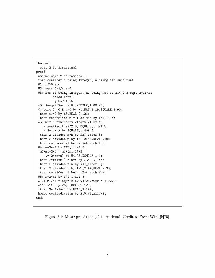
The Mizar system [58][75, §2] was introduced in 1978, comprising both the Mizar Languageand the Mizar Checker. The intent was to stay close to standard mathematical vernacular,so that the translation from textbook proofs would be straightforward. Still active today,it boasts one of the largest collections of formalized mathematics in its Mizar MathematicalLibrary (MML) [12]. Figure 2.1 gives a typical Mizar proof. Here we can see the verbose-declarative style of Mizar scripts, as each individual proof step is explicitly stated, as wellas a syntax which mimics a natural language pen-and-paper proof.

Proof Automation

Mizar closely resembles Isabelle’s proof document language, Isar [73], with the notableexception that there are no proof tools explicitly referenced in the proof text. Indeed, theonly two tools available to a Mizar proof author are justifications via by (simple automatedreasoning) or from (consequence of rule application). If a reasoning step fails, the onlyrecourse is to expand that step into sufficiently “obvious” steps for the Mizar system.

The rationale of this design choice is to ensure that Mizar proofs can be understoodindependently of the Mizar Checker. The disadvantage of this approach is that there is nocapacity for the author to provide proof strategies in order to extend the scope of obviousproof steps. The resulting proofs are therefore extremely verbose and require significantmanual effort to complete. The MML demonstrates that this is not a insurmountablehurdle for formalized mathematics, however it is unlikely to be effective in large-scalesoftware verification.

2.1.2 Nqthm and ACL2

Nqthm [18] originates in 1973 with a focus on having a high level of automation at the costof limited expressivity: formulas often need to be rewritten or "encoded" in the system [75].It distinguishes itself from fully automatic theorem provers by allowing users to guide theautomation with intermediate lemma suggestions. It is succeeded by ACL2 [40] whichcurrently supports an impressive range of formalizations from hardware verification to thefundamental theorem of calculus.

One criticism of ACL2 is that it fails to satisfy the ‘de Bruijn criterion’: there isno small trusted checker that independently validates proofs. Although Mizar fails thiscriterion as well, the extensive use of automated decision procedures in ACL2 places muchmore trust in the correctness of the system.

Proof Automation

ACL2 and Nqthm are both implemented as variants of Common Lisp, where a first-orderlogic is embedded as a term-rewriting system. The semantics of the language are encodedas axioms in its logic, identifying the process of both writing and verifying programs. Alllogical formulas and definitions are encoded as Lisp functions, with the intention that

7

theoremsqrt 2 is irrational

proofassume sqrt 2 is rational;then consider i being Integer, n being Nat such thatW1: n<>0 andW2: sqrt 2=i/n andW3: for i1 being Integer, n1 being Nat st n1<>0 & sqrt 2=i1/n1

holds n<=n1by RAT_1:25;

A5: i=sqrt 2*n by W1,XCMPLX_1:88,W2;C: sqrt 2>=0 & n>0 by W1,NAT_1:19,SQUARE_1:93;then i>=0 by A5,REAL_2:121;then reconsider m = i as Nat by INT_1:16;

A6: m*m = n*n*(sqrt 2*sqrt 2) by A5.= n*n*(sqrt 2)^2 by SQUARE_1:def 3.= 2*(n*n) by SQUARE_1:def 4;

then 2 divides m*m by NAT_1:def 3;then 2 divides m by INT_2:44,NEWTON:98;then consider m1 being Nat such that

W4: m=2*m1 by NAT_1:def 3;m1*m1*2*2 = m1*(m1*2)*2

.= 2*(n*n) by W4,A6,XCMPLX_1:4;then 2*(m1*m1) = n*n by XCMPLX_1:5;then 2 divides n*n by NAT_1:def 3;then 2 divides n by INT_2:44,NEWTON:98;then consider n1 being Nat such that

W5: n=2*n1 by NAT_1:def 3;A10: m1/n1 = sqrt 2 by W4,W5,XCMPLX_1:92,W2;A11: n1>0 by W5,C,REAL_2:123;then 2*n1>1*n1 by REAL_2:199;

hence contradiction by A10,W5,A11,W3;end;

Figure 2.1: Mizar proof that√2 is irrational. Credit to Freek Wiedijk[75].

8

the proof of a given statement can be automatically discovered by the proof system. Afailed proof attempt requires the user to modify the set of available lemmas, to guide theautomated proof search to a valid proof.

New automated reasoning procedures are given as transformation functions to thesimplifier, requiring that they produce a proof of equivalence to maintain logical soundness.These procedures can be arbitrarily complex, as they are simply Lisp functions, and areautomatically applied during the proof search.

2.1.3 LCF

The so-called ‘de Bruijn criterion’ for theorem provers [13] requires that the soundness ofthe system only depend on a small, trusted core. Often this is referred to as the proof kernelof the system: a module that is solely responsible for performing logical justifications.

The original LCF (Logic of Computable Functions) proof assistant [32] was one ofthe earliest provers that satisfies this criterion, while simultaneously providing the abilityto use automated reasoning procedures. LCF pioneered the notion of proof tactics andtacticals (i.e. operators on tactics) that can be still seen in its descendants today. A tacticcan perform arbitrarily complex computations on the proof state. A tactical proof isgenerally more interactive than either Mizar or ACL2: each tactic manipulates the proofstate, transforming it and presenting the result to the user. The proof is complete oncethe given series of tactic invocations successfully reduces the state to zero open proofobligations.

ML was invented for LCF as the Meta Language to implement tactics and other toolsaround the core logical engine. It is a fully-featured functional programming language,serving as both the implementation and proof language of LCF, with no formal distinc-tion between proofs, tool implementations or theory specifications. LCF inspired manyof the proof systems in use today. These LCF-style provers maintain logical soundnesswith a small, trusted kernel, while providing facilities for using and developing tactics forautomated reasoning.

2.1.4 HOL

The HOL (higher-order logic) family [75, §1] continues the LCF tradition with ML as themain integrating platform for all activities of theory and proof tool development (usingStandard ML or OCaml), however it replaces LCF’s Logic of Computable Functions withsimply-typed classical set theory. HOL provers provide only a bare-bones interface tothe ML top level by default, although different interface languages have been developed.This has been done as various “Mizar modes” to imitate the mathematical proof languageof Mizar (see Section 2.1.1), or as “SSReflect for HOL Light” that has emerged in theFlyspeck project, inspired by SSReflect for Coq [30].

Proof Automation

As in LCF, HOL tactics and tacticals are implemented in ML, which transform a givensubgoal state to build up a series of justifications for an initial formal hypothesis. The

9

full power of ML is always available to build advanced automated proof procedures asre-usable tools. HOL tactics work in the opposite direction to inferences in the core logic,which only allow deriving new facts from old ones.

This duality of backward reasoning from goals versus forward reasoning from facts isreconciled by tactic justifications: a tactic both performs the goal reduction and recordsan inference for the inverse direction. At the end of a tactical proof, all justifications arecomposed with the proof kernel to produce the final theorem. Programming errors in thetactic implementations could cause this final step to fail, i.e. if a proof step was taken thatcould not be logically justified.

Users of HOL are nearly always operating directly in ML, making the transition fromonly writing proofs to also developing proof tactics a natural progression. However thiscould also be seen as a disadvantage of the system: users are always exposed to its imple-mentation details, with few abstractions or conveniences when simply writing proofs.

2.1.5 Coq

Coq [75, §4] started as another branch of the LCF family in 1985, but with differentanswers to old questions regarding the relationship between proofs and programs. Coqimplements the Calculus of Inductive Constructions type theory as its core logic, wherea logical statement is a type and its corresponding proof is some term of that type. Astatement is therefore known to be true if its type is inhabited.

Similar to HOL, Coq provides a rich library of built-in proof tactics and tacticals fordeveloping proofs. A series of tactics in a Coq proof ultimately construct a final proofterm, which is formally justified by type checking. This type checking algorithm thereforealso serves as Coq’s proof kernel.

In contrast to HOL, the OCaml environment of Coq is not readily accessible for regularusers. Implementing a new Coq plug-in in OCaml requires that it be compiled and linkedseparately. If using the bytecode compiler, users may drop into an adhoc interactiveOCaml shell during a Coq session, however this is not accessible when using the defaultnative compiler. Coq users are therefore generally limited to its high level specificationand proof language. Custom proof automation is made available through several tacticlanguages, each designed for different applications and styles of proof development.

Proof Automation

Ltac is the untyped tactic scripting language for Coq [25], and has been successfully ap-plied in large Coq theory developments [21]. It has familiar functional language elements,such as higher-order functions and let-bindings. However, it contains imperative elementsas well, namely the implicit passing of the proof goal as global state. The main function-ality of Ltac is provided by a match construct for performing both goal and term analysis.Matching performs proof search through implicit backtracking across matches, attemptingmultiple unifications and falling through to other patterns upon failure. Although syn-tactically similar to the match keyword in the term language of Coq, Ltac tactics havea different formal status than Coq functions. Although this serves to distinguish logical

10

function application from on-line computation, it can result in obscure type errors thathappen dynamically at run-time.

Mtac is a recently developed typed tactic language for Coq [76]. It follows an approachof dependently-typed functional programming: the behaviour of Mtactics may be charac-terized within the logical language of the prover. Mtac is notable by taking the existinglanguage and type-system of Coq (including type-inference), and merely adds a minimalcollection of monadic operations to represent impure aspects of tactical programming asfirst-class citizens: unbounded search, exceptions, and matching against logical syntax.Thus the formerly separate aspect of tactical programming in Ltac is incorporated intothe logical language of Coq, which is made even more expressive to provide a uniformbasis for all developments of theories, proofs, and proof tools. Thanks to strong statictyping, Mtac avoids the dynamic type errors of Ltac. More recent work combines Mtacwith SSReflect [31], to internalize a generic proof programming language into Coq, inanalogy to the well-known type-class approach of Haskell.

This uniform proof language approach is quite elegant for Coq, but it relies on theinherent qualities of the Coq logic and its built-in computational approach. In contrast, thegreater LCF family has always embraced multiple languages that serve different purposes:classic LCF-style systems are more relaxed about separating logical foundations fromcomputation outside of it; potentially with access to external programs or network services.

SSReflect [30] is the common label for various tools and techniques for proof engineeringin Coq that have emerged from large verification projects by Gonthier. This includes asophisticated proof scripting language that provides fine-grained control over operationswithin the logical subgoal structure, and nested contexts for single-step equational rea-soning. Actual small-scale reflection refers to implementation techniques within Coq, forpropositional manipulations that could be done in HOL-based systems by more elementarymeans; the experimental SSReflect for HOL-Light re-uses the proof scripting language andits name, but without doing any reflection (this is neither possible nor required in HOL).

SSReflect emphasizes concrete proof scripts for particular problems, not general proofautomation. Scripts written by an expert of SSReflect can be understood by the same,without stepping through the sequence of goal states in the proof assistant. General toolsmay be implemented nonetheless, by going into the Coq logic. The SSReflect toolboxincludes specific support for generic theory development based on canonical structures.

Canonical Structures were later introduced by Gonthier [31] as a method of instrument-ing automation within the logic while avoiding the use of explicit tactic invocations. Henotes that tactics, being essentially untyped, operate as arbitrary proof state transformers.This makes it difficult to determine when a change will affect the execution of a tactic.There is no possibility to specify the intended behaviour of a tactic, let alone verify it. Byusing canonical structures, the unification/type inference algorithm of Coq is coerced intoexecuting decision procedures while generating types, effectively lifting the automationas a first class object. The “execution” of the procedure, however, is intrinsically linkedwith the implementation of the unification algorithm, which is not specified formally andperforms poorly when used for this application. Moreover, the automation is constrainedto logic-style programming, which limits its utility.

11

2.1.6 The Lean Theorem Prover

Lean is a more recent entry into the space, with a strong focus on automation andinteroperability with other systems [24]. Similar to Coq, Lean implements the dependenttype theory of Calculus of Inductive Constructions to unify both proof and type checking.Proofs can be constructed as a mix of both tactics and declarative Mizar-style keywords.

Lean offers the ability to specify a trust level when invoked, allowing for relaxed cor-rectness checking by invoking macros that sidestep the proof kernel. A high trust levelmay use heavily optimized macros in order to support rapid prototyping and proof devel-opment, while a trust level of zero forces macro expansion to ensure that all proofs aresound.

2.1.7 Isabelle

Isabelle was originally introduced as another Logical Framework by Paulson [56], to allowrapid prototyping of implementations of inference systems, especially versions of Martin-Löf type theory. This was provided by establishing a minimal meta-logic, known asIsabelle/Pure, and allowing end-users to establish their own object-logics. Many haveemerged since: e.g. ZF set theory, FOL and HOLCF, however most applications today aredone in the object-logic Isabelle/HOL.

Isabelle is written in Standard ML, descended from ML which was originally developedfor use in LCF. Isabelle’s Pure logic descends from the LCF-style of interactive theoremproving, limiting logical inferences to a small trusted core. Before Isar, proofs in Isabellewere simply ML programs, whose type signature guaranteed that they were limited toperforming valid logical inferences according to Isabelle/Pure.

Isar was first seen in 1999 [70] and was introduced as a “declarative” language forproof text. Its design was heavily influenced by Mizar, with an aim to overcome its lack ofextensibility and scalability. Isar’s support for unstructured proofs (proof scripts) provideda convenient launching point for porting existing proofs from ML. Today nearly all Isabelleproofs are written in Isar, while ML is used to add functionality by defining new keywordsor proof methods.

Proof Automation

As in other LCF-style systems, proofs in Isabelle can be represented a series of tactics thatreduce a proof state to having zero open proof obligations. Similar to HOL, the soundnessof these proofs is guaranteed by representing theorems as an abstract datatype that canonly be transformed by a small proof kernel. In contrast to HOL, however, the proof stateitself is represented as a theorem, avoiding the need for tactic justifications after the proofis completed.

Isar introduced the concept of proof methods (see Section 3.3) as an interface forinvoking Isabelle’s tactics in structured proofs. Each method defines its own syntax,which may be arbitrarily complex, for controlling the underlying tactics and dynamicallyextending Isabelle’s proof context (see Section 3.4.4) to implicitly provide hints and facts.

12

Proof Automation

Tactics in Lean can be used both in proof blocks or invoked by the elaborator in order tocompute missing subterms required to make a term type-correct. As in other LCF systems,Lean tactics are arbitrarily complex programs that ultimately appeal to the underlyingproof kernel to guarantee soundness.

Lean supports defining meta-programs outside the axiomatic foundations of the sys-tem. Specifically a meta-definition may recurse infinitely, and have access to a set ofmeta-constants for interacting with Lean itself. Similar to Coq’s Mtac, meta-programs inLean can be used to define new proof tactics by representing a tactic as a state monadover proof subgoals.

2.2 Relationship to Isabelle/Eisbach

Tactics in Isabelle are written in ML, and proof methods have also historically been ex-clusively written in ML. In this thesis, we present Eisbach (see Chapter 5): a high levelproof method language for Isabelle/Isar. Of the languages presented in this chapter, Eis-bach most closely resembles Coq’s Ltac: it is a untyped scripting language for writingautomated reasoning procedures by combining existing tools and providing control flowthrough matching. This is no accident, as the accessibility and flexibility of Ltac has madeit a popular choice for many Coq proof authors and thus serves as a good reference pointfor a successful tactic language.

Eisbach distinguishes itself from Ltac in two important ways: convenient access toadvanced functionality via ML and ad-hoc extensibility through context data. Eisbachbenefits greatly from Isar’s ML integration, allowing for language extensions to be im-plemented as needed without requiring modifications to Eisbach or Isar. In contrast toLtac, Eisbach’s match (see Section 5.2.4) enjoys no special status in the language: it isimplemented in ML as a standalone proof method. Although it is considered a core partof Eisbach as it provides critical functionality, match also demonstrates what is possiblefor end-users to implement in their own proofs. Additionally, in Section 5.2.7 we give anexample of ad-hoc integration with ML, where a fact-producing ML function is used as amatch target to expose previously-inaccessible functionality to Eisbach methods. Similarfunctionality is not readily available in Coq, as interfacing with OCaml directly requiresseparately compiling custom Coq plug-ins.

In Coq, the Hint command allows users to define sets of hint databases to be auto-matically applied by the auto tactic. Eisbach’s integration with Isar’s named theoremsmakes similar functionality easily available to any custom proof method, allowing post-hoc method extensions through managed collections of facts in the proof context. This ismotivated by the knowledge management issues that become apparent in large scale proofengineering, where multiple extensive databases of theorems need to be effectively used byproof authors. Eisbach allows custom proof methods to easily provide structured accessto user-defined named theorems, automatically using them where applicable rather thanrequiring users to manually search through thousands of irrelevant theorems. In Chapter 7we show how this functionality can be used to define a core algorithm for a non-trivial

13

proof method, while allowing large numbers of additional calculational and terminal rulesto be incrementally proven and provided later.

2.3 Proof Engineering

In the previous sections, we saw how different proof systems approached both their logicalfoundations and availability of custom proof automation. Using these systems effectively tobuild scalable and maintainable proofs is the core challenge of proof engineering. Proof en-gineering requires both having effective tools that minimize the cost and effort of buildingproofs, while also collecting data on these proof artefacts to better predict and understandhow effort will scale to further proofs.

Differences between proof systems, and differences in proof styles within those systems,have made it difficult to establish best practices in this field. Although there are manyanalogous problems in software engineering, they have their own unique challenges in thecontext of proof engineering.

2.3.1 Proof Maintenance

Proofs in a machine-checked system must be consistently maintained, where maintenancecycle can be triggered in response to changes to the proof system itself (e.g. the semanticsor syntax of a command), a dependant proof or definition, or some external artefact (e.g.verified source code).

Bourke et al. report [17] on challenges faced in the maintenance of large scale proofs inthe L4.Verified (see Section 3.5) and Verisoft [7] projects. They note the proof activity for asingle module in L4.Verified, showing bursts of proof development followed by long periodsof maintenance. A large portion of this maintenance is performing manual refactoring taskson existing proofs, most frequently necessitated as a result of failing to avoid duplicationduring the initial proof development. The Levity tool was developed during the scope ofthe project to automatically reorganize lemmas.

Proof Refactoring

Restructuring proof is similar in many ways to code refactoring. However, in cases whereuntyped automated reasoning methods are applied as part of a proof script, it becomesnearly impossible to assign static semantics to the proof. Additionally in systems such asIsabelle, proofs are processed with respect to some context which implicitly affects the be-haviour of automated methods without being represented syntactically (see Section 3.4.4).

Iain Whiteside gives a rigorous treatment of proof refactorings with respect to theformal proof language HiProofs and tactic language HiTac [74]. A small set of refactoringsare considered, with a focus on reorganizing lemmas and unfolding automatic procedureswithin proofs. The significant drawback with this approach is that the semantics of existingproof systems need to be applied to HiProofs/HiTac for the proposed refactorings to haveany use.

Alma et al. present two methods for dependency extraction in Coq and Mizar [6]with the motivation of fast refactoring of large mathematical libraries and instrumenting

14

automated reasoning techniques. The significant difficulty cited is removing unnecessarydependencies, where the theorem prover has used more than is necessary to complete agiven proof.

Ringer et al. use automation to compute reusable patches to proofs and specifica-tions [57]. They note the inherent brittleness of formal proofs, as seemingly minor changesoften have wide-reaching effects, and advocate for increased tool support to shift the bur-den of change away from proof authors.

Eisbach can be effectively used to reduce the maintenance overhead of proofs by pro-viding a convenient interface for expressing duplicated reasoning. A significant aspect ofproof maintenance is repairing proofs after a small specification or proof change has causeda particular manual proof step to fail that is repeated in multiple separate proofs. WithEisbach, this step can be easily factored into a re-usable proof method.

2.3.2 Proof Generalization

Modularization of code is a significant part of proper software engineering, grouping con-cerns into consistent sub-components and managing their interaction through abstractinterfaces. The motivation is clear from a development and maintenance perspective: adistinct logical module can easily be re-used when its functionality is needed by anothercomponent, reducing duplication and maintenance overhead. Often this is supported by ageneralizing refactoring, in which a piece of code is parametrized to make it more globallyuseful [29].

Similarly, large proof developments must be organized to reduce duplicated reasoningand lemmas are generalized to support more uses. Isabelle’s locales [10] allow for defini-tions, proofs and other tools to be generalized over terms and assumptions. The modulesystem in Coq [22] provides similar functionality to produced parametrized theories.

Felty and Howe implemented a prototype proof system designed to generalize tactic-based proofs to instrument proof-by-analogy [27]. Their approach operates on the explicitproof trees generated by the system, rather than the proof text given by the user. Grovand Maclean [34], in a more recent work, propose a generalization technique based onProof Strategies, which leverages techniques from artificial intelligence. They develop anotion of goal types which capture goal features, matching against them to apply relevanttactics.

Eisbach is a natural extension to Grov and Maclean’s proof strategies, as they ulti-mately require some native proof tool in order to manipulate the goal state of the under-lying prover. Providing a suite of specialized Eisbach methods can therefore enhance thegranularity of these strategies.

2.3.3 Empirical Evaluation of Proof Artefacts

Although the space of large-scale proof development and engineering is growing, therehave been correspondingly few empirical investigations. In formal verification, research todate has concentrated on measuring formal specification of programs and the relationshipbetween these measures and system implementations.

15

Formal Specifications

In Olszewska and Sere [55] the authors report on their use of Halstead’s software sciencemodel [36] for the measurement of Event-B specifications. They used this framework tomeasure the “size of a specification, the difficulty of modelling it, as well as the effort”.The specification metrics developed were seen as useful descriptors of the specificationsstudied when applied in the DEPLOY project [3].

Some research has also been carried out on other specification metrics. In 1987 Samsonet al. [59] investigated metrics that might aid in cost prediction for software developed.They use McCabe’s cyclomatic complexity metric [51] and lines of code to measure theimplementation of a small system and measures of operators and equations to measurethe HOPE formal specification. Although their sample size was small, they found a re-lationship between their measures of the specification and implementation. Tabareh’smasters thesis [67] contained an investigation of relationships between specification andimplementation measures. A number of specification metrics were defined for Z specifi-cations. These were size-based metrics such as lines of code and conceptual complexity;structure based metrics such as logical complexity; and semantic based metrics such asslice-based coupling, cohesion and overlap. In a more recent paper Bollin [16] evaluatedthe use of specification metrics of complexity and quality in a case study comprising morethan 65,000 lines of Z specification text. Staples et al. [65] analysed the relationship be-tween the specification and implementation sizes for API functions in L4.verified, findingthat the formal specification sizes correlated much more strongly than COSMIC FunctionPoint count [38].

In Chapter 4 we define a general metric for measuring the size of a formal statement byanalysing its dependency graph, and present a novel idealisation of this metric, useful inthe presence of over-specified statements, by considering the content of its proof to prunethe graph of unnecessary dependencies. We find that this idealised size correlates muchmore strongly with the size of the eventual proof of the statement, and therefore is likelya better estimation of its complexity.

Proofs and Formal Verification

Andronick et al. [8] provide a comprehensive retrospective analysis of the L4.verifiedproject, citing the “middle-out” development process as a key factor in its success. Adescriptive process model is given, highlighting the major phases of the project and theiterative nature of its development, along with the evolution of the size of each majorartefact. Despite the data collected, the authors admit that “We do not yet have a goodunderstanding of what to measure in formal verification projects.” They note that thelessons learned from this analysis were qualitative and not immediately useful for devel-oping “decision-making models to inform project management judgments”.

Later, Staples et al. [64] extracted size and effort data from L4.verified to understandtheir relationship. They found a “strong linear relationship” between the effort spent ona given proof (in person-weeks) and its eventual proof size (in lines of proof script), forboth projects and individuals.

Jeffery et al. [39] propose a research agenda for “empirical study of productivity in

16

software projects using formal methods”. With support from prior literature, they identifyover thirty research questions that require additional data. They note that althoughhigh-level concepts are shared between software engineering and formal methods, such as“size, effort” and “rework”, the nature of their measurement in proof engineering will besignificantly different. In this agenda, they identify following question:

How are characteristics of formal specifications, properties, or code related toeffort in formal proofs?

The study in Chapter 4 attempts to address this by investigating several verificationprojects to establish the relationship between the size of a formal statement and its formalproof. Finding a quadratic relationship between statement and proof size, we hypothesizethat the effort required to verify software with current techniques will increase quadrati-cally with the size of its code.

This study, and another question identified by Jeffery et al. motivates the developmentof Eisbach:

How can we best combine interactive proof and proof automation to achievehigh proof productivity during initial proof development and subsequent proofmaintenance?

In Chapter 7 we address this question in the context of Eisbach by implementing a setof proof methods to automate previously-manual proofs in L4.verified.

2.4 Conclusion

In this chapter, we gave a brief overview of different proof systems and their approachesto proof automation. Some systems, like Mizar, expose very little or no functionalityfor providing additional automated reasoning procedures. Proofs are therefore extremelyverbose and manual, but can be independently understood by a human reader. Othersystems, like ACL2, are almost entirely automated. Users may extend the space of au-tomated strategies available, but their application occurs as an extension to its standardproof search rather than as an interactive process. Neither Mizar nor ACL2 satisfy the ‘deBruijn criteron’: they lack a small, trusted proof checker. In ACL2 this is of particularconcern, given its high reliance on automated reasoning.

LCF-style provers like Coq, HOL and Isabelle provide a small proof kernel that allmanual and automated proofs must use. This allows for powerful automated proof tools,called tactics, to be developed without compromising trust in the proofs that use them. InHOL, most tactics are developed in its implementation language ML, while Coq providesseveral high-level tactic languages. These languages have different advantages with respectto usability, expressibility and static guarantees, however the majority of custom Coqtactics use Ltac, its untyped scripting language. Eisbach provides similar functionality toIsabelle/Isar, focusing on large scale proof engineering and extensibility.

Proof engineering is the discipline of developing proofs in these systems to be scalableand maintainable, while also providing empirical analysis of the artefacts and processes

17

involved. We showed existing work on tools for maintaining, refactoring and generalizingproofs. We also presented several studies on the relationship between formal specificationsand code size, as well as some larger retrospective studies on the successful L4.verifiedproject. We find, as Jeffery et al. [39] note in their research agenda, that a lack ofempirical analysis in proof engineering has made it difficult to build good models for proofeffort.

In the next chapter we focus on Isabelle, its high-level proof language, Isar, and thestructure of the L4.verified project. These form the basis for the later chapters, wherewe investigate the L4.verified proofs in an empirical analysis of proof size vs. specificationsize in Chapter 4, design Eisbach as an extension to Isar in Chapter 5, and ultimatelyuse Eisbach in Chapter 7 to implement a set of proof methods that automate previously-manual proofs from L4.verified.

18

Chapter 3

Background

In the previous chapter we have seen a wide array of interactive proof systems, each witha different emphasis on the accessibility of writing custom proof tools. In this chapter weshift our focus to Isabelle, discussing foundations and the state of the art in automating itsproofs. Isabelle is implemented in Standard ML, along with a rich ecosystem of powerfulautomation tools. Isar, Isabelle’s proof document language, provides access to this proofautomation at a high level of abstraction, allowing end users to focus on the logic ofproofs rather than implementation details of the system. However, it is also designedto be extensible: users may define their own Isar commands in ML for both generatingspecifications and automating proof procedures. The result has been an ever-growing suiteof Isabelle functionality that is easily accessible via Isar.

Readers familiar with Isabelle/Isar can skip to Section 3.5, which introduces theL4.verified project.

Chapter Outline

• Introduction to Isar. Section 3.1 gives a brief overview of the core concepts ofIsabelle/Isar.

• Isabelle/Pure. Section 3.2 covers Isabelle’s meta logic and proof kernel

• Proof Methods. Section 3.3 is an overview of Isabelle’s existing proof methods andmethod combinators

• Isar Revisited. Section 3.4 presents a more in-depth discussion on relevant Isarconcepts for this thesis.

• L4.verified. Section 3.5 provides an introduction to the L4.verified project

• The Archive of Formal Proofs. Section 3.6 briefly introduces Isabelle’s Archiveof Formal Proofs

• Formatting Remarks. Section 3.7 discusses the formatting of Isar input and out-put in this thesis

19

3.1 Introduction to Isar

Isar stands for Intelligible, semi-automated reasoning [71]. It provides a high-level interfaceto Isabelle’s proof engine with a suite of commands for driving the proof process whilesimultaneously documenting the intuition of the proof author. As Isar itself is devoid ofcomputation, proof methods (see Section 3.3) are used to interact with Isabelle’s proof statein order to formally discharge proof obligations. Internally, proof methods use Isabelle’sproof kernel (see Section 3.2.3) to ensure soundness, and most built-in methods simplyprovide a syntactic interface to some Isabelle tactic.

3.1.1 A Simple Proof

In Isar, a proof begins when some command (i.e. lemma) initiates a proof block, statingthe assumptions and conclusion of a desired fact.lemma IsarSimpleExample:assumes asm1 : A =⇒ B

and asm2 : Ashows B

In this example, A and B are arbitrary boolean terms that are fixed for the duration of theproof. The assumptions are given with the assumes keyword asm1 (A =⇒ B) and asm2(A). These are local facts that can be used in the scope of this proof. The conclusion,given with shows, is the goal of the proof.

The proof then proceeds as a series of interactive commands to show that the conclusionis true under the stated assumptions. The apply command can be given to evaluate proofmethod expression on the current proof state. This transforms the goal, either dischargingit or introducing new subgoals. One of the simplest methods is rule that resolves theconclusion of the current goal against the conclusion of a given rule.

In this case, we can use rule twice to apply both of our assumptions to the goal andcomplete the proof.

apply (rule asm1 )apply (rule asm2 )

Once the proof is complete and no proof obligations (subgoals) remain, we can use thedone command to conclude.

doneUpon successful completion of the proof, the fixed terms in the lemma are generalized intoschematics (see Section 3.2.2) and the stated assumptions are inserted as antecedents tothe conclusion. In this case the resulting IsarSimpleExample lemma is (?A =⇒ ?B) =⇒?A =⇒ ?B and is now generally available in further proofs.

3.1.2 The Languages of Isabelle

The previous example showed the modus-ponens rule of Isabelle’s meta-logic, demonstrat-ing the three main sub-languages of Isabelle/Isar:

20

• The Isar command language. Proof commands, such as apply, drive the proofstate and interactively present the user with information about it.

• The term language of Isabelle/Pure. Terms are parsed as arguments to Isarcommands as the formal basis of the lemma statement and proof. Here A and Bare free variables in the term language, and =⇒ is a constant, representing meta-implication from the meta-logic of Isabelle/Pure.

• Isar’s proof method expressions. Proof methods discharge the formal obliga-tions of the proofs, appealing to the meta-logic of Isabelle/Pure.

In the next section, we present the core concepts of Isabelle/Pure as they relate to proofand proof method development in Isabelle, and in Section 3.3 we present a more compre-hensive overview of proof methods.

3.2 Isabelle/Pure

3.2.1 Meta-logic Connectives

Isabelle/Pure is a higher-order logic, serving as a framework for performing Natural De-duction. Pure is based on simply-typed λ-calculus (modulo αβη-conversions), with aspecial type prop defined as the type of propositions. Every logical statement in Pure is aprop and is constructed with the two meta-logical connectives,

∧(universal quantification)

and =⇒ (implication). Additional meta-connectives are derived from these primitives,such as ≡ (meta-equivalence) and &&& meta-conjunction. Pure connectives have a lowsyntactic precedence, compared to connectives from object logics, such as ∀ or ∧ fromHOL (see Section 3.2.4). The Pure connectives outline inference rules declaratively, forexample:

• conjunction introduction, traditionallyA BA ∧ B

, is: A =⇒ B =⇒ A ∧ B

• well-founded induction is: wf r =⇒ (∧x . (

∧y . (y , x ) ∈ r =⇒ P y) =⇒ P x ) =⇒ P a

3.2.2 Terms

A term in Isabelle/Pure is constructed from the following primitives:

Bound Variables in Lambda Abstractions. A lambda-abstraction represents a func-tion in Isabelle, where bound variables refer to function arguments that are providedpostfix, e.g. (λx y . x =⇒ y) A B evaluates to A =⇒ B . Universal quantification

∧is syn-

tactic sugar for the higher-order function Pure.all, where∧x . P x is equivalent to Pure.all

(λx . P x ).

Constants. A constant is a term with a globally-fixed (potentially polymorphic) type,usually provided with one or more definitional axioms (i.e. my_equiv ≡ (λx y . (

∧P .

P x =⇒ P y))). Object-logics may define their own interfaces for ensuring introduced

21

definitional axioms are sound, and provide advanced functionality for constructing non-trivial definitions (e.g. for recursive functions).

Schematic Variables. A schematic variable is logically equivalent to a variable that isoutermost meta-universally quantified, and is represented with a ? prefix. Isabelle/Pureprovides lifting functions to convert between these equivalent forms, for example the stan-dard form of

∧x . (

∧y . P x y) =⇒ Q x is (

∧y . P ?x y) =⇒ Q ?x .

When a given rule is resolved against the current goal, Isabelle’s unifier is used to firstcalculate valid instantiations for schematics appearing in both the rule and the goal inorder for them to match.

Free Variables. A free variable is arbitrary-but-fixed within a given context (see Sec-tion 3.4.4), with optional type restrictions. Outside the context (e.g. when a proof iscompleted), a free variable can be generalized into a schematic. By default, most Isarcommands will interpret any unknown terms (i.e. not constant or bound) as free vari-ables, and proof commands (i.e lemma) will declare them as fixed for the duration of theproof.

Types

Terms in Isabelle/Pure have an associated type, where an explicit type constraint is rep-resented with infix notation: term :: type. The syntax of functions is infix, i.e. _ ⇒_. Logical statements have the special type prop, with meta-connectives used as prop-producing functions (i.e. =⇒ :: prop ⇒ prop ⇒ prop). Types are constructed from thefollowing primitives:

Type Constructor. Similar to a constant term, a type constructor is globally definedand takes zero or more type arguments. For example, the function type (_ ⇒ _) takestwo type arguments: the domain and range types, while prop takes zero arguments.

Schematic Type Variable. Similar to a schematic term variable, a schematic typevariable represents a polymorphic type that can be instantiated. It is syntactically repre-sented with a ? ′ prefix. For example, meta-universal quantification is polymorphic in thequantified variable, and has the type (? ′a ⇒ prop) ⇒ prop.

Free Type Variable. Similar to a free term variable, a free type variable representsan arbitrary-but-fixed type for some context, syntactically represented with a ′ prefix.Outside this context, free type variables can be generalized into schematics. For example,if we start a proof with lemma

∧x . P x =⇒ P x , the bound variable x is assigned the

fresh, free type ′a. Once the proof is complete, x is generalized into a schematic term (i.e.P ?x =⇒ P ?x ) and ′a is generalized into a schematic type (i.e. ? ′a).

Type variables (free and schematic) can be additionally declared as a particular sort, whichrestricts how they may be instantiated.

3.2.3 Proof Kernel

Isabelle’s inference kernel follows the LCF tradition of providing an abstract ML type(thm) that represents the type of “true” statements, with respect to the underlying meta-

22

logic, object-logic and any axioms used. A thm can only be created by ultimately appealingto the primitive interface of the kernel, although powerful tools can be built using thisinterface. The core internal data member of a thm is its underlying cterm: another abstractML type representing a term that has been type-checked by the kernel. A thm can thereforebe thought of as a term with an implicit certificate that it is a type-correct prop which hasbeen derived from the primitive inference rules of Pure.

Rather than maintain an auxiliary data structure for the proof goal state in ML, asin the original LCF system, in Isabelle it is simply represented as a single thm. A proofof some hypothetical statement C begins with the trivial fact C =⇒ C , provided as aprimitive from Pure. This proof proceeds by manipulating the subgoal structure of thisthm (i.e. its antecedents) and eventually reducing it to having zero subgoals, i.e. =⇒ C , orsimply C. Administrative goal operations, e.g. shuffling of subgoals or restricted subgoalviews, work by elementary inferences involving =⇒ in Isabelle/Pure.

An intermediate goal state with n open subgoals has the form H 1 =⇒ ... H n =⇒ C,each with its own substructure H = (

∧x . A x =⇒ B x ), for zero or more goal parameters

(here just x ) and goal premises (here just A x ). Following [56], this local context is implic-itly taken into account when natural deduction rules are composed by lifting, higher-orderunification, and backward chaining. Often, long chains of meta-implication (as usuallyseen when pretty-printing subgoals) will be presented with a condensed syntax: (A =⇒ B=⇒ C =⇒ D) ≡ ([[A; B ; C ]] =⇒ D).

Isabelle tactics due to [56] follow the idea behind LCF tactics, but implement thebackwards refinement more directly in the logical framework, without the replay tacticjustifications (which is still seen in HOL or Coq today). A tactic is therefore simply anML function from thm ⇒ thm list, which transforms an intermediate proof state thm intoan unbounded lazy list of results. Tactic failure returns an empty set of results, while mul-tiple results represents different backtracking options. Simple tactics include: backwardsreasoning by applying a rule to the conclusion of a subgoal, forwards reasoning from apremise of a subgoal, and solving a subgoal by matching its conclusion with one of itspremises. LCF-style tacticals combine and transform tactics, some common tacticals are:sequential composition, alternative composition, repeated application, optional applica-tion, and applying a given tactic to all subgoals. A traditional tactic-style proof scriptchains together a series of tactics to reduce a proof state to having no open subgoals.

Although the framework of Isabelle has changed significantly over the past few decades,the proof kernel has remained largely undisturbed. The Isar proof document language pro-vides an alternative view on these primitive concepts, managing most of the administrativedetails behind-the-scenes while ultimately appealing to this small trusted core.

3.2.4 Isabelle/HOL

Isabelle’s Pure logic is designed as a minimal implementation of an inference system,allowing users to establish their own object logics within it. Among the many logicsthat have emerged, Isabelle/HOL hosts the majority of the current Isabelle applications.Although Eisbach (see Chapter 5) and most of the tools implemented in Chapter 6 arecompatible with other object logics, we present them in this thesis only in the context ofIsabelle/HOL.

23

Table 3.1: Comparison of Isabelle’s Pure and HOL connectives.Connective Name Pure Syntax HOL Syntax

Universal Quantification∧x . P x ∀ x . P x

Implication P =⇒ Q P −→ QEquivalence P ≡ Q P = QConjunction P &&& Q P ∧ QDisjunction - P ∨ Q

Existential Quantification - ∃ x . P xNegation - ¬ P

HOL formulas are of type bool, where the special purpose function Trueprop :: bool⇒ prop is used to embed them into the Pure logic. This is known as an object-logicjudgement, and is implicitly inserted/hidden by the term parser/pretty printer when op-erating within HOL. Each Pure connective has an equivalent HOL interpretation (shownin Table 3.1), however HOL additionally defines existential quantification, disjunction andnegation. Furthermore, HOL defines the constants True and False and axiomatizes the lawof excluded middle (i.e. ∀P . P = True ∨ P = False).

3.3 Proof Methods

As seen in Section 3.1.1, proof methods can be invoked during an Isar proof with theapply keyword to transform the goal state. An apply does not insist that the proof becompleted, and outputs the resulting proof state to the user after successfully evaluatingthe given method. Further apply commands may follow to continue the proof, until it iseventually concluded by the command done. This chain of method invocations is oftenreferred to as a proof script, where determining its logical content requires inspecting eachintermediate goal state.

Isar additionally supports producing and presenting, human-readable formal proofs.These structured proofs explicitly state the assumptions and intermediate conclusions ofeach step, referring to proof methods to discharge intermediate proof obligations. Con-cluding a structured proof block a method is usually done with the by command, whichevaluates one or two given proof methods, requiring that they successfully solve the goal.

The majority of the proofs presented in this thesis are largely unstructured, with somestructured Isar elements (e.g. explicit lemma assumes or proofs concluding with by).

We can consider two rough classifications of methods: basic methods that perform asingle reasoning step or technical adjustment, and automated methods that use heuristicsand search to both simplify and solve goals. Here we present a small selection of proofmethods, seen in the later chapters of this thesis.

3.3.1 Basic Proof Methods

• rule fact1 ... factn Backward reasoning from the conclusion. Resolves the conclu-sion of the current subgoal with the conclusion of each theorem in the given facts,

24

backtracking over each result. The assumptions of the applied theorem are thenintroduced as subgoals. Example: use with conjI ([[?P ; ?Q ]] =⇒ ?P ∧ ?Q)

• erule fact1 ... factn Forward reasoning by eliminating an assumption. Resolves theconclusion of the current subgoal with the conclusion of each theorem in the givenfacts, as well as resolving the first assumption of the theorem with an assumptionin the current subgoal, backtracking over each result. The remaining assumptionsof the applied theorem are then introduced as subgoals. Example: use with conjE([[?P ∧ ?Q ; [[?P ; ?Q ]] =⇒ ?R]] =⇒ ?R)

• drule fact1 ... factn Forward reasoning from an assumption. Resolves an assumptionof the current subgoal with the first assumption of each theorem in the given facts,backtracking over each result. The remaining assumptions of the applied theoremare then introduced as subgoals. Example: use with conjunct1 (?P ∧ ?Q =⇒ ?P)

• assumption Discharge the current subgoal by resolving it with one of its assumptions,backtracking over each result.

3.3.2 Automated Proof Methods

• simp add: fact1 ... factn Simplify the current subgoal through rewriting, poten-tially solving it. A large database of facts and processes are implicitly retrievedfrom the context, which can be managed through various declaration attributes(e.g. rule[simp]) or optionally provided in-place after add:.

• auto simp: fact1 ... factn intro: fact1 ... factn elim: fact1 ... factn Simplify allsubgoals, additionally applying known introduction (backwards) and elimination(forward) rules from the context and attempting classical reasoning solvers.

3.3.3 Method Combinators and Backtracking

In general, apply and by accept proof method expressions, basic proof methods combinedusing method combinators. Unlike tacticals, there are only a minimal set of combinatorsprovided. These support backtracking over method results, where the end of each ap-ply is the first successful result of all combined methods. The standard proof methodcombinators are as follows:

1. Sequential composition of two methods with implicit backtracking: the expression“method1, method2” applies method1, which may produce a set of possible results(new proof goals), before applying method2 to all possible goal states produced bymethod1. Effectively this produces all results in which the application of method1

followed by method2 is successful.

2. Alternative composition: “method1 | method2” tries method1 and falls through tomethod2 when method1 fails (yields no results).

3. Suppression of failure: “method? ” turns failure of method into an identity step onthe goal state.

25

4. Repeated method application: “method+” repeatedly applies method (at least once)until it fails.

5. Goal restriction: “method [n]” restricts the view of method to the first n subgoals.

The subsequent example illustrates a proof method expression with combinators:lemma P ∧ Q −→ Pby ((rule impI, (erule conjE)? ) | assumption)+

Informally, this says: “Apply the implication introduction rule, followed by optionallyeliminating any conjunctions in the assumptions. If this fails, solve the goal with anassumption. Repeat this action until it fails.”

This method expression is applicable to more than one proof, and indeed will solve aclass of propositional logic problems involving implication and conjunction. In Chapter 5we will see how Eisbach can be used to define a new method using this method expression,and how it can be refined into a general-purpose propositional logic solver.

3.4 Isar Revisited

In this section we present a small selection of additional Isar functionality, relevant to thefollowing chapters of this thesis.

3.4.1 Facts and Theorems

Although Isabelle’s proof kernel operates on theorems (i.e. a thm), Isar operates on lists oftheorems called facts. Individual members of a fact may be selected by an explicit index(i.e. my_fact(n) for selecting the nth theorem of my_fact).

For example, a lemma may prove multiple theorems and store them in a single fact:lemma my_theorems: A B C

thm my_theorems — A, B, C

thm my_theorems(1) — Athm my_theorems(2) — Bthm my_theorems(3) — C

3.4.2 Definitions

In Isabelle, new constants can be declared with optional type restrictions, and then defi-nitional axioms can be added to allow the constant to be rewritten as its body. Isabelle’sprimitive definition package enforces the logical consistency of any declared definition (i.e.avoiding cyclical dependencies).

The most straightforward access to this functionality is via the definition Isar com-mand, which simultaneously declares a new constant and its definitional axiom. e.g.:definition is_nonzero :: int ⇒ boolwhere is_nonzero x ≡ x 6= 0

26

This declares a new constant is_nonzero with the type restriction int ⇒ bool and simul-taneously produces a new fact named is_nonzero_def (is_nonzero ?x ≡ ?x 6= 0).

3.4.3 Records

The record command, provided by Isabelle/HOL, allows for defining record types, withautomatically generated field-update syntax and corresponding lemmas. e.g.:record machine_state =program_counter :: intmemory :: int ⇒ int

lemma((|program_counter = 1, memory = X |) :: machine_state)(|program_counter := 0|) =(|program_counter = 0, memory = X |)by simp

3.4.4 Proof Context

The structured proof context provides general administrative structure to complementprimitive thm values from the kernel. The context tracks the scope of fixed terms, fixedtypes, and structured assumptions.

Revisiting our first example from Section 3.1.1, at the start of the proof, the contextis locally augmented with the assumptions asm1 and asm2 as well as the fixed variablesA and B.lemma IsarSimpleExample:assumes asm1 : A =⇒ B

and asm2 : Ashows B

Once this proof concludes, proving B, the inner (proof) context is compared to the outercontext to determine how to properly finalize the result. Since asm1 and asm2 are onlydeclared in the inner context, they are added as antecedents to the conclusion (i.e. [[A =⇒B ; A]] =⇒ B). Additionally, since A and B are only fixed in the inner context, they canbe generalized into schematics to produce the final theorem: [[?A =⇒ ?B ; ?A]] =⇒ ?B).The inner context is then discarded, and the resulting rule is added to the set of knownfacts in the current (outer) context with the name IsarSimpleExample.

thm IsarSimpleExample — [[?A =⇒ ?B ; ?A]] =⇒ ?B

Declaration Attributes

The proof context may also be augmented with arbitrary tool data, providing both globaland local information. This is generally managed through declaration attributes, whichadd or remove rules from tool-specific collections (i.e. rule[simp] to add Simplifier rules tothe context).

For example, we can declare local assumptions as simp so they are picked up by thesimp method during a proof.

27

lemmaassumes A: A

and B : Bshows A ∧ B by (simp add : A B)

lemmaassumes A[simp]: A

and B [simp]: Bshows A ∧ B by simp

Once a proof concludes, the effects of any locally-applied declaration attributes are dis-carded.

Named collections of dynamic facts can be declared with the named_theorems com-mand, with corresponding attributes to add or delete entries (see Section 5.2.1 for moredetails.)named_theorems my_simps

lemmaassumes A[my_simps]: A

and B [my_simps]: Bshows A ∧ B by (simp add : my_simps)

So far these attributes have all had local effects, persisting only for the duration of a singleproof. A declaration can instead be made global (with respect to the outer context) byappending it to the name of a lemma.lemma my_AB[my_simps]: A =⇒ B =⇒ A ∧ B by simp

Additionally, the declare command allows for applying declaration attributes to existingfacts.declare my_AB[my_simps]

Alternatively, the lemmas can declare multiple lemmas simultaneously.lemmas [my_simps] = my_AB TrueI

3.4.5 Rule Attributes

Previously (see Section 3.4.4) we saw declaration attributes used to modify Isabelle’sproof context. In this section we will cover rule attributes, which have the same syntax asdeclaration attributes, but instead perform in-place rule transformations.

The where and of attributes

These attributes are used to instantiate schematic variables in existing rules. With whereeach variable instantiation is named, while of takes an list of terms and instantiatesschematics by order of their appearance in the given rule.

28

lemma [[A; B ]] =⇒ A ∧ Bthm conjI — [[?P ; ?Q ]] =⇒ ?P ∧ ?Q

thm conjI[where P=A and Q=B ] — [[A; B ]] =⇒ A ∧ Bthm conjI[of A B ] — [[A; B ]] =⇒ A ∧ B

apply (rule conjI[of A B ])apply assumptionapply assumptiondone

The THEN and OF attributes

These attributes are used to perform in-place composition of existing rules. With OFthe given facts are unified against the assumptions of the source rule. Conversely, THENunifies the source rule against the first assumption of the given rule.lemmaassumes A: A

and B : Bshows A ∧ B

thm conjI — [[?P ; ?Q ]] =⇒ ?P ∧ ?Q

thm conjI[OF A] — ?Q =⇒ A ∧ ?Qthm A[THEN conjI] — ?Q =⇒ A ∧ ?Q

thm conjI[OF A B ] — A ∧ B

apply (rule conjI[OF A B ])

done

3.4.6 Isabelle/ML

Isar supports embedding ML as a sub-language, where logical entities (i.e. terms andtheorems) can be referred to via antiquotations [72]. The ML command can be used toexecute arbitrary ML, optionally defining new variables or functions.

For example, we can define an ML tactic that attempts to solve the goal by resolvingit with TrueI (i.e. the goal is trivially True).

ML 〈val trivial_tac = resolve0_tac [@{thm TrueI}] 1〉

Here the thm antiquotation has retrieved the fact TrueI from the current context andembedded it in the tactic. We can then use this directly with the special-purpose tacticproof method, to invoke an ML tactic as a proof method.lemma True by (tactic 〈trivial_tac〉)

Additionally, various Isar “setup” commands take an ML function as an argument in orderto define new Isar tools (e.g. attributes or methods, see Section 3.4.5 and Section 3.3). Wecan use method_setup to define a new proof method from this tactic.

29

method_setup trivially_True = 〈Scan.succeed (fn ctxt => SIMPLE_METHOD trivial_tac)〉

lemma True by trivially_True

This natural integration with ML allows Isar to enjoy a significant amount of ad-hoc ex-tensibility. However it also allows for many more opportunities for unexpected behaviour.lemma Falseapply (tactic 〈fn _ => Seq .single @{thm TrueI}〉)

No subgoals!

In this example it appears that we’ve successfully proven False. Fortunately an error israised when we try to finish the proof.done

Lost goal structure:True

In this example we’ve destroyed the internal subgoal structure (see Section 3.2.3) of theproof by replacing it with simply True. Although this now appears to be a completedproof, with zero open subgoals, it does not prove the intended goal of False. Isar thereforethrows an error when attempting to finalise the proof. This particular pitfall can beavoided by using only built-in tactics that maintain Isabelle’s subgoal structure; howeverthis demonstrates that, with ML, much more care must be taken to manage concepts thatare otherwise abstracted away by Isar.

3.5 L4.verified

The L4.verified project [42] produced a formal, machine checked proof of the full functionalcorrectness of the seL4 microkernel, down to the binary level, followed by proofs of securityproperties about the kernel. seL4 is a small operating system kernel, designed with explicitgoals of high performance, formal verification, and secure access control. The kernel itselfcomprises 10, 000 lines of C code, while its corresponding proofs have grown to over 500, 000lines of Isabelle.

The L4.verified proofs feature heavily in this thesis, as they are to-date among thelargest proofs in both Isabelle and interactive theorem proving at large. In Chapter 4 weuse several of its sub-projects in an empirical analysis analysing proof effort scalability,and in Chapter 7 we present case study where Eisbach is used to build proof methods thatautomate previous-manual proofs from L4.verified.

In L4.verified, the primary original result was refinement between the C implemen-tation and its abstract specification of seL4. Roughly, a specification A is said to refinespecification C if all possible observable behaviours of C are subsumed by the possiblebehaviours of A, given the same inputs (see Chapter 7 for more details). For seL4, thisimplies that the C implementation will always adhere to the abstract specification (undersome assumptions). Desirable properties of the abstract specification, such as avoiding

30

invalid memory accesses and maintaining invariant properties, are then easily shown tohold of the C implementation via refinement.

More recent work has extended this refinement stack in both directions; from showingthat the final compiled binary is a faithful representation of its C source [62], to buildingmore abstract specifications for reasoning about initialized systems on top of seL4 [19].This allows for both greater trust in the verification result, and extends the scope of whatkinds of properties can be proven about the kernel.

3.5.1 L4.verified specifications

Rather than directly prove refinement between the C and abstract specification, the projectwas instead divided into three sub-specifications:

The Abstract Specification (ASpec) The abstract specification is manually writtenin Isabelle/HOL as a functional specification for the seL4 microkernel. It is formalizedas a non-deterministic state monad (see Section 7.1.2) in order to abstract away imple-mentation details. For example, the concrete scheduling algorithm is abstracted into non-deterministically choosing a runnable thread. Additionally some kernel data structures,such as the capability derivation tree, are abstracted into pure Isabelle/HOL functions.

The Executable Specification (ExecSpec) In the early design phases of L4.verified,an initial prototype for seL4 was built in Haskell. This prototype was designed to be binarycompatible with the C implementation by modelling hardware interactions as statefultransformations of a state monad(see Section 7.1.2). The model is sufficiently accuratesuch that it can be executed on the QEMU emulator [14], which allowed for design decisionsto be rapidly tested in the early days of development. This Haskell kernel serves as anatural intermediate specification between the C and abstract. Rather than formalize thesemantics of Haskell in Isabelle/HOL, however, it was more straightforward to generatemonadic functions directly from the Haskell source. This resulted in a shallow embeddingof the specification, which is better supported by the automation in Isabelle/HOL and issignificantly easier to reason about.

The C Implementation and Specification (CSpec) The seL4 microkernel is writtenin a slightly restricted subset of C in order to facilitate translation into Isabelle/HOL andverification. To provide this C source with a formal semantics, it is preprocessed and givento Norrish’s C-to-Isabelle parser [69]. This parser performs a conservative translation of Csemantics into SIMPL [60], a minimalistic imperative language defined in Isabelle/HOL.The resulting SIMPL program (often referred to as the C specification) then serves as theprimary verification artefact for L4.verified within Isabelle.

3.5.2 L4.verified refinement stack

Abstract invariants (AInvs) This proof contains the definition and proof of a collec-tion of invariant properties about the abstract specification (ASpec). These were initiallydeveloped to ultimately support the executable-to-abstract (Refine) proof, and later used

31

during the Access and InfoFlow proofs. It is supported by the wp method, developed toperform weakest-precondition style reasoning over monadic specifications (see Section 7.1).

Executable-to-abstract refinement (Refine) This proves that the executable spec-ification (ExecSpec) is a refinement of the abstract specification (ASpec). It is combinedwith the result of CRefine to ultimately prove that the C implementation (CSpec) satisfiesthe abstract specification. Its refinement calculus previously lacked an automated proofmethod, prompting the case study presented in Chapter 7.

C-to-executable refinement (CRefine) This proves that the embedded C implemen-tation (CSpec) is a refinement of the executable specification (ExecSpec). It is supportedby the semi-automated ctac method, used for transforming proof states in the refinementcalculus and optionally generating verification conditions for refinement.

3.5.3 Additional L4.verified proofs

Access Control (Access) The proof of functional correctness was followed by a proofthat seL4 enforces integrity [63]. Phrased as an invariant property, integrity places anupper bound on the possible effects of each kernel invocation across security domains.

Information Flow (InfoFlow) Building on the Access proof, InfoFlow proves thatseL4 enforces confidentiality [52]. This is proven by reasoning about multiple programtraces, placing an upper bound on what information is read during a kernel invocationand ensuring that security domains can avoid leaking confidential information.

3.6 The Archive of Formal Proofs

The Archive of Formal Proofs (AFP) [43] is a collection of proofs in Isabelle, aimed atfostering the development of formal proofs and providing a place for archiving proof de-velopments to be referred to in publications. The AFP counts over 400 entries. Twoof the largest software verification proofs from the AFP are JinjaThreads [44] and SAT-SolverVerification [45], used in the empirical study presented in the following chapter.

JinjaThreads Jinja is a Java-like programming language formalised in Isabelle, witha formal semantics designed to exhibit core features of the Java language architecture,and formal proof of properties such as type safety and compiler correctness. JinjaThreadsextends this development with Java-style arrays and threads, and shows preservation ofthe core properties.

SATSolverVerification This is a proof of correctness of several modern SAT solvers,including termination proofs as well as a large number of lemmas about propositional logicand CNF-formulae.

32

3.7 Formatting Remarks

3.7.1 Fonts

When presenting Isar input and Isabelle’s output in this thesis, we use three fonts toindicate the status of the given text.

• For Isar commands and minor keywords we use bold serif . Example commandsare lemma, term and done. Example minor keywords are assumes, shows anduses.

• When formatting both terms and inner Isar syntax, we use italics to indicate thatcontent is either locally scoped (e.g. a bound or arbitrary-but-fixed variable) or thatit is some other minor content (e.g. a flag or text argument).

• We use sans serif to indicate that content is some fixed constant, e.g a proven lemma,or a defined term or method.

In the example from Section 3.1.1, the formatting of the line apply (rule asm1 ) indicatesthat apply is an Isar command, rule is a defined method (as opposed to amethod parameteras in Section 5.2.3), and that asm1 is a locally-scoped assumption.

For readability (seen primarily in Chapter 7), Isar keywords will occasionally be omit-ted from the text when the meaning is clear.

3.7.2 Interactive Proof State

The proof of IsarSimpleExample in Section 3.1.1 does not show Isabelle’s output duringthe proof process. Each command (i.e. lemma, apply, and done) produces interactivefeedback to inform the author of Isabelle’s proof state. Additionally, diagnostic commands(i.e. term and thm) allow the user to inspect logical elements of the current state.

To show Isabelle’s output interactively in this thesis, we present the output from agiven command between two horizontal lines. Revisiting our previous example, we maychoose to show the proof state at each step.lemma IsarSimpleExample:assumes asm1 : A =⇒ B

and asm2 : Ashows B

1 . B

Here we see that the current proof state has a single subgoal, to prove B. We apply asm1with rule to perform backwards reasoning on this goal.apply (rule asm1 )

1 . A

33

This has resolved the conclusion asm1 with the current goal conclusion B, and now requiresthat we show A. At any point, we can use the diagnostic command thm to inspect thecontent of facts.thm asm1

A =⇒ B

thm asm2

A

We can apply asm2 to solve the current goal and finish the proof.apply (rule asm2 )

No subgoals!

At this point the proof is complete and we conclude with done.done

For the sake of brevity, we may instead give Isabelle’s output as inline comments in theIsar text (prefixed by — ).lemma IsarSimpleExample:assumes asm1 : A =⇒ B

and asm2 : Ashows B — 1 . Bapply (rule asm1 ) — 1 . A

thm asm1 — A =⇒ Bthm asm2 — A

apply (rule asm2 ) — No subgoals!done

34

Chapter 4

Empirical Analysis of Proof EffortScalability

In this chapter, we investigate the relationship between the formal specification of a soft-ware verification proof development and the size of its eventual formal proof. We present anempirical analysis of proofs from both L4.verified (see Section 3.5) and Isabelle’s Archiveof Formal Proofs (see Section 3.6), finding a consistent quadratic relationship in theseproof developments, between the size of the formal statement of a property, and the finalsize of its formal proof.

Combined with previous work by Staples et al. [64], which shows a linear relationshipbetween the effort required to complete a proof and its final size, this suggests a quadraticrelationship between the formal specification of a program and the effort required for itsproof.

Informally this quadratic relationship can be justified by a common structure seen insoftware verification proofs: where a desired set of n properties must be verified over klines of code, requiring n×k lines of proof. This presents a clear scalability challenge forverifying larger systems: as the number of lines grows, reducing the required effort ofverifying each line becomes critical.

Later, in Chapter 5 we present Eisbach, a high-level extensible proof method languagefor Isabelle/Isar that allows proof authors to reduce duplicated reasoning and manual proofeffort. In Chapter 7 we use Eisbach in a case study to develop a set of proof methods forperforming automated reasoning in the refinement calculus of L4.verified [23]. We demon-strate the effectiveness of these methods by applying them to several existing L4.verifiedproofs to drastically reduce their size and complexity. By eliminating a significant manualcomponent of these proofs, the resulting infrastructure becomes much more capable ofscaling to both new, larger programs and subsequent iterations of L4.verified.

Acknowledgements

This chapter is based on work that previously appeared at the International Conferenceon Software Engineering, 2015 [47], in collaboration with Toby Murray, June Andronick,Ross Jeffery, Gerwin Klein and Mark Staples. The author was the primary contributor

35

to this paper. Specifically, his contributions were: the development of a proof metriccollection framework for Isabelle, the collection of all the presented proof data, and theidealised metric detailed in Section 4.3.

Chapter Outline

• Motivation and Summary. Section 4.1 presents the need for empirical analysisof proof artefacts for proof engineering.

• Approach and Measures. Section 4.2 describes the precise measures used in thisinvestigation.

• Measures in Isabelle. Section 4.3 specializes the measures from Section 4.2 toIsabelle.

• Data Collected. Section 4.4 presents the raw data from the investigation and itsanalysis.

• Results and Discussion. Section 4.5 reflects on the data and the metrics used.

• Conclusion. Section 4.6 summarizes and puts the discovered quadratic relationshipof specification size and proof size into the context of this thesis.

4.1 Motivation and Summary

Despite a number of recent successes in software verification, a major hurdle has been ageneral lack of experience in large scale proof development. This makes it difficult to drawgeneral conclusions about how proof effort scales, a critical question in proof engineering.

This suggests that empirical analysis of successful verification projects is needed in or-der to understand the scalability of existing approaches. Earlier work [65] has showed theneed for a better understanding of how to measure artefacts in formal methods, to informcosts and estimation models. An analysis of the existing literature [39] revealed a short-age of empirical studies to provide industry with validated measures and models for themanagement and estimation of formal methods projects. As Stidolph and Whitehead [66]state:

experienced formal methodologists insist that cost and schedule estimation tech-niques are unsatisfactory and will remain so until a large body of experiencebecomes available.

In other words, the absence of many successful large-scale verification projects makesit impossible to build a generally-applicable predictive model for required effort. Wecan, however, build explanatory models from the few existing suitable projects in orderto understand existing scalability challenges. This paves the way for building predictivemodels as more experience becomes available, while informing the development of newproof techniques and technologies.

36

Previously [64], Staples et al. analysed proof productivity, and revealed a strong linearrelationship between effort (in person-weeks) and proof size (in lines of proof script), forprojects and for individuals. In this investigation we examine the inputs to softwareverification projects: formal statements of the properties to be proved about programs,and formal specifications of the programs. Our goal is to identify measures of these formalstatements and specifications that relate to the final size of their interactive proofs.

We present results of an empirical analysis of a large number of proofs written inIsabelle. We measure the size of each lemma, in terms of the total number of conceptsneeded to state it, and compare that to the total number of lines used to prove it. Weanalysed four large sub-projects from L4.verified (see Section 3.5) as well as two proofsfrom the Archive of Formal Proofs (AFP) (see Section 3.6). From these 6 projects, weanalysed a total of 15,018 lemma statements and associated proofs, covering a total ofmore than 215,000 lines of proof.

We find a consistent quadratic relationship between statement size and proof size, withthe coefficient of determination (R2) for the quadratic regressions varying from 0.154 to0.845. One of the four sub-projects from L4.verified stands out with a lower R2 and a sig-nificant collection of outliers, with proof sizes much smaller than would be expected giventhe statement size. Investigation revealed that these outliers were caused by over-specifiedlemma statements (see Section 4.2.4), with large constants mentioned unnecessarily, ef-fectively inflating their statement size. To test this hypothesis, we defined an idealisedmeasure for statement size that is an approximation of its minimum size. Using this mea-sure greatly strengthens the relationship between statement size and proof size across allthe projects, with R2 between 0.73 and 0.937. This implies that there is a very strongquadratic relationship between statement size and proof size, when statements are notunnecessarily over-specified.

This supports a hypothesis made by Cock et al. regarding the scalability of theirapproach in L4.verified, stating “We hypothesise that the effort for the whole verificationso far was quadratic in the size of the kernel.” [23] Microkernel code is highly non-modularby nature, and so verification is dominated by proving invariants. Each invariant needsto be preserved by each feature, which in turn relies on and modifies data structures usedby other features. Our current work provides empirical evidence for this hypothesis, bycorrelating proof size to statement size.

4.1.1 Limitations

In general, it is not possible to create a universally applicable model that relates a formalstatement to its proof size or required proof effort. For example, Fermat’s Last Theoremcan be trivially stated, and yet over 350 years passed after its initial conjecture before aproof was found1.

A universal model limited to only software verification is impossible as well. Wecould encode Fermat’s last theorem as a verification problem (i.e. a program that assertsan + bn 6= cn for any inputs where n > 2). If the integer sizes are unbounded, verifyingthis program would be at least as difficult as proving the original theorem.

1Aside from Fermat’s hypothetical proof, of course.

37

Conversely, we could construct a degenerate 100,000 line program with extremely com-plex source code, but where the main entry point immediately returns without calling anyother functions. This would be trivial to verify (assuming this is the intended behaviour),but would likely appear to require significant effort by any metric.

With that said, we posit that most software to be verified will not contain such edgecases, and indeed must be well-formed in order for a human to be intuitively convinced ofits correctness. The bulk of the work will therefore not be in solving any hard problems,but rather iterating each desired property over the entire program’s structure. From this,we hypothesize that by gathering data on existing, successful verification projects, we cangain insight into how real-world proof effort will scale.

4.2 Approach and Measures

We can consider two primary artefacts when discussing a proof development in an inter-active theorem prover: a specification S and its corresponding proof P . For example, informal verification S comprises the formalized program code (with corresponding seman-tics) along with desired correctness properties for the software. To prove S in an ITP, wemust provide a proof P in the proof language of the ITP, most likely appealing to resultsfrom existing libraries or intermediate lemmas. The set of all definitions, intermediatelemmas, and the final proof P of S form the proof development that ultimately establishesthe property expressed in S. This S is then referred to as the top-level statement orproperty of the proof development.

In order to successfully develop a proof of S it must be decomposed into sub-components that can be stated and proven as independent lemmas. Each of these lemmastherefore contains a fragment of the overall specification as its formal statement. Thefinal proof P is the culmination of these lemmas, which ultimately describe all of thecomponents of S.

In this section we describe a general measure for the size of a formal statement of alemma, as well as the size of its formal proof.

4.2.1 Proofs and Specifications

A proof development in an ITP is comprised of definitions, lemma statements and proofs ofthose lemmas. Definitions are used to introduce new constants and give them semantics,such as function specifications, program invariants or data structures. These definitionsare given in the term language of the theorem prover, which has a precise syntax and se-mantics. Lemma statements relate constants, positing a fact that is then proved. Similarto definitions, lemma statements are written in the term language. Term and proof lan-guages vary significantly between theorem provers, however they all share similar traits.A term can express logical statements, with connectives (e.g. conjunction, implication)and quantifiers (e.g. universal, existential). Proof languages have syntax for appealing toautomated reasoning tools and previously proven results. A proof, in this context, is asequence of appeals which eventually demonstrate that a lemma statement is true.

As a running example, consider the following definitions of two new constants C and

38

E, which mention some propositions A and B from a previous proof development. Theyalso depend on the exclusive-OR operator ⊕ and the usual logical connectives.

C ≡ (¬A) ∨ (¬B)E ≡ B⊕ C

The constants implicitly form a dependency graph. A constant c directly depends onanother constant c′ if c′ appears in the definition of c. This represents an edge in theconstant dependency graph from node c to node c′. In our example, E directly dependson B, C, and the ⊕ connective. We say that c depends on c′′ if c′′ is reachable from cin the constant dependency graph. In other words, c′′ must be defined at some point inorder to define c. In our example E depends on all of A, B, C, and the three connectives⊕, ∨ and ¬.

Similarly lemmas also implicitly form a dependency graph: a lemma l directly dependson another lemma l′ if l′ is used to justify some step in the proof of l. Lemma l is thensaid to depend on l′′ if at any point l′′ had to be proved for the proof of l to hold. Inour example, one can state the following lemmas to be proved (where the −→ operator islogical implication).

E −→ (A ∨ ¬B) (4.1)E ∧ B −→ A (4.2)

The truth of Formula 4.1 and Formula 4.2 simply relies on the definitions of E and C andstandard propositional logic. Their Isabelle proofs might look like the following:lemma Eq1: E −→ (A ∨ ¬B)unfolding E_def C_defapply (rule HOL.impI)apply (elim xorE HOL.disjE HOL.conjE)apply (subst (asm) HOL.de_Morgan_disj)apply (subst (asm) HOL.not_not)apply (rule HOL.disjI1)apply (elim HOL.conjE)apply assumptionapply (rule HOL.disjI2,assumption)+done

lemma Eq2: E ∧ B −→ Aapply (metis Eq1)

doneIt is not necessary to understand these proofs. We observe, however, that the proof of thelemma Eq1 refers only to facts from theHOL proof development, which defines the HigherOrder Logic of Isabelle (see Section 3.2.4), as well as the facts that capture the definitionsof C and E, C_def and E_def respectively, plus the fact xorE that in this example hasalready been proved in an existing proof development on which it builds.

39

4.2.2 Proof Size

In our analysis we consider a given lemma and relate its statement size to its proof size.Formally we define the size of the proof of a lemma l to be:

Proof size of lemma l: the total number of source lines used to state andprove l, excluding definitions.

Note that this includes the proofs of all lemmas that l depends on. We exclude definitiondeclarations (such as C_def) because, although they are part of the proof source, we areinterested in the total number of new source lines written to complete stages (2) and (3)of a proof development; definition declarations are all written in stage (1).

We refine this notion of size slightly by only counting source lines from a particularproof development D. We call this the proof size of l with respect to D, defined as follows.

Proof size of lemma l with respect to proof development D: the totalnumber of source lines required to state and prove l, excluding definitions, aswell as lemmas and proofs outside of D.

The reason that we contextualise proof size this way is because proof development iscumulative, and new proofs often build on old ones. For example, a proof development D,proving the correctness of Dijkstra’s algorithm, would appeal to lemmas and definitionsfrom an existing proof development G, a formalisation of graph theory. G would providea definition of a graph, edges, paths, and would have lemmas proved about reachability.When measuring the size of the proof of a lemma from D in order to gauge its effort, onewould consider the lemmas in G to have come at zero cost, and not take their size intoaccount. More precisely, in general we measure the size of any proof of a lemma from aproof development D with respect to D, in order to exclude from its size any pre-existinglemmas on which it depends.

In our example, all the facts used in the proof of Eq1 come from an pre-existing proofdevelopment except C_def and D_def that are the definitions of C and D respectively.Thus none of the direct dependencies of the proof of Eq1 are counted when computingits size. The size of the proof of Formula 4.1 therefore is just its immediate size (i.e. 11lines), while the proof of Formula 4.2 would be measured as its immediate size summedwith the size of Formula 4.1 (i.e. 3 + 11 = 14 lines).

4.2.3 Raw Statement Size

Here we define a measure for the statement of l that we found correlates well with theproof size of l as defined above:

Raw statement size for lemma l: the total number of unique constantsrequired to write the statement for l, including all of its dependencies, recur-sively.

“Unique” specifies that each constant is counted at most once per statement. This measure,importantly, is computable after stage (1) in the proof development as it only requiresdefinitions to have been written, and does not depend on proofs. We refer to this as a

40

statement’s raw size. This is distinguished from the statement’s idealised size, introducedlater.

Similarly to proof size, it often makes sense to measure statement size with respectto some proof development D. Doing so excludes all constants that fall outside of D.However, while we measure the size of a proof in proof development D with respect to Ditself, it often makes more sense to measure statements in D with respect to a larger proofdevelopment D′ that includes D. In the example of the previous section, when measuringthe size of Formula 4.1, we might choose to count the sizes of A and B, even though theseconstants have been defined in a pre-existing proof development, and even though proofsabout A and B in this pre-existing development will not be counted in the size of the proofof Formula 4.1. The reason is that the effort of proving a new fact about a constant c(here e.g. A) might be highly impacted by the size of c even though it has been definedin a pre-existing development. In the context of the seL4 proofs we observed this effectto be extremely strong, where most statements referring to seL4’s abstract specification(defined in a separate proof development)would have proofs which follow the structure ofthe abstract specification and carry the complexity of reasoning about it.

In the example of the previous section, assume we choose to measure the size of For-mula 4.1 and Formula 4.2 with respect to the entire proof development down to the axiomsof the logic, i.e. including the definitions of A and B and all the operators. Assume that Aand B are complex constants with sizes 100 and 200 respectively. For simplicity we assumetheir dependencies are disjoint, so C would have a size of 1 + 100 + 200 + 1 + 1 = 303,where we add 1 for C itself, the size of A, the size of B and then the size of ¬ and ∨ (weassume for simplicity that they are defined axiomatically). We can then calculate the sizeof E as 1 + 1 + 303 = 305, by adding 1 for E itself, 1 for ⊕ (also assumed to be definedaxiomatically) and then the size of C. Note that we do not add the size of B, as it hasbeen considered already when calculating the size of C, and we are only counting uniqueconstant dependencies. Then Formula 4.1 would have a size of 305 + 1 = 306, where wecount the size of E and the size of −→ (the other constants being already considered inthe size of E). Similarly Formula 4.2 would have a size of 306.

Note that both proof size and statement size are inherently recursive; the proof sizeof l includes the size of its dependent lemmas, and the statement size of l is based onits dependent definitions. No attempt is made to measure the immediate size of anylemma, as this is far too susceptible to fluctuations in individual proof style. In ourexample, Formula 4.2 has a small immediate proof size (3 lines), but would be given thesame statement size as Formula 4.1. By considering each in terms of all of its dependencieswe get a much more robust measure.

4.2.4 Idealised Statement Size

Most lemmas make stronger assumptions than are actually necessary. In particular, alemma might have a concrete term where an abstract one will suffice: the statement “1is odd” is less general than the statement “2n + 1 is odd”, which has an abstract term“2n+1” in place of the concrete term “1”. It is the job of the proof engineer to decide theappropriate level of generality for a lemma, based on its intended use. In cases where aconstant with a large definition is included unnecessarily, we observe a large discrepancy

41

between statement and proof size.In our example, consider the statement ¬C ∨ C. Suppose it was proved in one step by

appealing directly to the law of excluded middle, an axiom of HOL in Isabelle. The rawsize of this statement is 303 + 1 + 1 = 305. This is an over-estimation of the statement’scomplexity because the statement mentions C unnecessarily — C could be abstractedwithout affecting the proof. Doing so (by replacing the constant C by a variable x) wouldyield a statement with size of just 2 (1 for each logical connective), a much better indicationof its proof complexity.

In practice, over-specificity can save effort in provers like Isabelle, as it can aid auto-mated reasoning by simplifying higher order unification, a primitive procedure in Isabelle.Additionally it is not often worth the effort to generalise a lemma that will only be usedonce. As a result, it is common to see many over-specific lemmas in large proof develop-ments.

To address this, we introduce idealised statement size. The idealised size for the state-ment of some lemma l is the size it would have been given had it been stated in its mostgeneral terms. More precisely, it is defined as follows.

Idealised statement size for lemma l: the raw size of the statement of lhad it been abstracted over all possible constants such that l’s proof remainsvalid.

Note that we apply this recursively, conceptually removing mentions of redundant con-stants in all dependant constants of l’s statement. The idealised statement size of l isalways smaller or equal to the raw size of l, as it may only remove unnecessary constantsfrom measurement. Unfortunately, computing this size is undecidable as it would requirea precise analysis of why l is true. We show how it can be approximated in Section 4.3.3.

4.3 Measures in Isabelle

The definitions given in the previous section abstracted away from any specific theoremprover. Here we explain how we compute these measures for Isabelle.

4.3.1 Measuring Proof Size

Previously, in Section 3.1 we covered the structure of a proof in Isabelle/Isar. Each Isarproof begins with a proof command (e.g. lemma) and ends with a terminal command (e.g.done) once the proof is complete. The lemma statement as described in Section 4.2.2 isboth the stated conclusion and any assumptions.

To measure proof size, we distinguish Isabelle fact (see Section 3.4.1) from the morespecific Isabelle lemmas. Although Isabelle makes no formal distinction between these two,we consider a lemma to be a fact which has been explicitly stated by a proof engineer,with a provided Isabelle/Isar proof. A fact is more general: it is a statement that has beenproved by any means. This includes lemmas, but also all the statements automaticallygenerated and internally proved by Isabelle. For example, defining a recursive functionf requires a proof of its termination. In many cases this termination proof can be done

42

automatically with no manual invocations of tools. This fact is implicitly used in anylemma l that reasons about f , but it does not have a proof size that can be measured insuch a way that would correspond to the effort required to prove it (since it is automatic).Therefore, when computing the size of the proof of a lemma l, we will only count the proofsizes of used lemmas. Lemmas are the only facts whose proofs require substantial humaneffort, therefore they are the only ones relevant to our investigation.

For a given lemma l in Isabelle we say that the lines between the beginning andending keywords (inclusive) constitute the proof of l. The immediate size of l is thereforesimply its line count. Then we compute all the lemmas which l recursively depends onand add their sizes to get l’s total size. Here we only count unique lemmas: if multipledependencies of l depend on some l′, we only count the size of l′ once. We compute lemmadependencies by examining proof terms produced by Isabelle [15], where a proof term isthe internal formal representation of a proof. The total size of l with respect to some proofdevelopment D considers all lemmas outside of D to have size 0. Simply put, for eachproof development, lemmas not from that development (e.g. pre-existing library lemmas),do not contribute to the measured size of proofs.

This measure approximates the proof size of l as described in Section 4.2.2. It isincomplete, however, as it does not include source lines which must exist for l to be valid,but for which this dependency relationship is not easily found. For example, the proofof l may depend on certain syntax existing, declared with one line using the notationkeyword. This is not factored into the total size of l. The impact of this on the validity ofthe measured proof size is assumed to be minimal, as the size of Isabelle proof developmentsis dominated by proof text.

4.3.2 Measuring Raw Statement Size

In Section 3.4.2 we saw how new constants could be introduced to Isabelle with Isar. Inter-nally these definitional commands create simple definitions based on the user specification,proving canonical facts for interpreting them. In our running example, the definition ofC introduces the new name C with body (¬A) ∨ (¬B), and a new fact C_def for thestatement C = (¬A) ∨ (¬B).

To measure the size of a given lemma statement S as described in Section 4.2.2 werecursively inspect all definitions mentioned in S. The number of unique definitions tra-versed will be the size of S according to this measure.

4.3.3 Approximating Idealised Statement Size

In Section 4.2.4 we introduced idealised statement size as a refinement of raw statementsize. Although computing the idealised size of S is, in general, undecidable, it can beapproximated by examining the finished proof of S.

Intuitively, if S refers to C but the defining fact C_def of the constant C does notappear in the dependency graph of the proof of S, this means that the truth of S does notdepend on the definition of C, and that S could be rewritten by replacing the constantC by a variable x. We therefore exclude the size of C when computing the approximateidealised size of S. For instance, the approximate idealised statement size of the statement

43

¬C∨ C, proved by appealing directly to the law of excluded middle without using C_def,is 2.

More generally, for each constant c, we have a set of defining equations. These areIsabelle facts which are the canonical interpretation of c. In the case of simple definitions,this is just the equation that was given when c was defined (such as C_def). To computethe idealised size of a statement S, we exclude all the constants whose defining equationsare never used in the proof of S. This will always be an over-approximation of the idealisedsize of S, but is at worst the original statement size.

This approximation of idealised statement size cannot be a leading predictor of proofsize, as it requires stage (3) of the proof to be complete. However, it is useful when tryingto build an explanatory model for understanding the relationship between statement sizeand proof size. The implications of using this measure are discussed in Section 4.5

4.4 Data Collected

We applied our exploratory analysis to six projects: (1) four top-level statements fromL4.verified, and (2) two proof developments in the Archive of Formal Proofs.

4.4.1 L4.verified Proofs

Previously (see Section 3.5) we outlined the structure of L4.verified. We applied thesemeasures to the AInvs, Refine, Access and Infoflow proof developments, taken from thepublic release of the seL4 proofs [68]. The statements measured for each proof develop-ment are all the dependencies of its top-level statement, computed with respect to thatdevelopment. The statement sizes for these proofs are computed with respect to the wholeseL4 verification development, where the large kernel specifications are defined.

AInvs: The top-level statement in this proof depends on both the abstract specifica-tion for seL4 (ASpec) and the abstract invariants (invs). We measured 2,790 lemmas fromAInvs, including the top-level statement with a raw size of 1,292, ideal size of 949 andproof size of 32,214 lines (measured as described in Section 4.3).

Refine: The top-level statement depends on the abstract specification (ASpec) andthe executable specification (ExecSpec), as well as a corresponding global invariant foreach of them. Refine builds on AInvs, but we compute the proof sizes for Refine withrespect to itself. That is, proofs from AInvs do not contribute to the size of proofs fromRefine. We measured 4,143 lemmas from Refine, including the top-level statement with araw size of 2,398, ideal size of 1,746 and proof size of 67,856 lines.

Access: The top-level statement depends on ASpec, the definition of integrity (see Sec-tion 3.5.3), as well as invs. Similar to Refine, we only measure Access proofs with respectto itself, taking proofs from Refine and AInvs for granted. We measured 724 lemmas fromAccess, including the top-level statement with a raw size of 1,395, ideal size of 1,083 andproof size of 8,116 lines.

InfoFlow: The top-level statement depends on ASpec, the definition of integrity, andinvs. Additionally it includes a more involved discussion of program execution traces.As previously done, proof sizes from InfoFlow are measured with respect to itself. We

44

Table 4.1: R2 and equations for Figure 4.1 and Figure 4.2

Proof Name Size Used R2 Equation f(x) = a · x2 + b · x+ ca b c

AInvs raw 0.845 0.02579 -8.181 394.9idealised 0.937 0.04325 -4.399 100.4

Refine raw 0.724 0.01198 -5.355 519.1idealised 0.799 0.01737 2.365 <2.2e-16

Access raw 0.735 0.0032 -1.112 86.45idealised 0.889 0.006039 -0.915 57.36

InfoFlow raw 0.154 -0.0003736 1.743 <2.2e-16idealised 0.73 0.007893 -3.652 260.4

JinjaThreads raw 0.457 0.05631 -16.46 472.9idealised 0.694 0.1166 -16.04 281

SATSolverVerification

raw 0.798 1.711 -65.43 375.7idealised 0.802 4.123 -77.52 223.7

measured 1,665 lemmas from InfoFlow, including the top-level statement with a raw sizeof 2,029, ideal size of 1,323 and proof size of 19,579 lines.

4.4.2 Proofs from the AFP

The Archive of Formal Proofs (see Section 3.6) is a public collection of proofs in Isabelle.We applied these measures to two of its largest software verification proof developments.

JinjaThreads: We measured 5,215 lemmas from JinjaThreads, including the top-levelstatement with a raw size of 579, ideal size of 453 and proof size of 39,821 lines.

SATSolverVerification: We measure the proof with respect to the FunctionalImple-mentation theory, an implementation of a SAT solver within Isabelle’s HOL. We measured481 lemmas from SATSolverVerification, including the top-level statement with a raw sizeof 99, ideal size of 57 and proof size of 21,788 lines.

4.5 Results and Discussion

For each of the six projects analysed, we computed the statement size and proof size ofall of its lemmas, using the measures described in Section 4.3. As explained, we used twovariants for the statement size: a raw measure and an idealised measure, where the latterrepresents what the size of the statement would be if stated in its most general form.

The results are given in Figure 4.1 for the raw measure and in Figure 4.2 for theidealised measure. The analysis demonstrates a consistent quadratic relationship betweenstatement size and proof size across all the projects, with a stronger relationship whenusing the idealised measure. The respective R2 and equations of the regression lines aregiven in Table 4.1. We now discuss the results in detail.

45

●

●

●

●

●

●

●

●

● ●

●●●

●

●●●● ●●

● ●

●● ●●●

●

● ●●●● ●

●

●

●●

●

●

●

●

●

●

●●●

●●●● ● ● ●●

●

●●●●● ●●● ●

●●●

●●●●●●●●●●●

●

● ●●● ● ●●● ●●● ●●●●

●

●

●

● ●

●

●

●

●● ●●●●●●●●●●● ●●●●● ●●● ● ●●●●●●●● ● ●●●

●

●●● ● ●●●

●

●●●

●

●●

●

●●●●●

●●●● ●● ●● ●●● ●●●●●●●● ●●● ●● ● ●●●●●● ●● ● ●●●

●

●● ●●● ●● ●●

● ●●

●

●●●● ●● ●●●● ●●●●●●●●●●●● ●●● ●●●● ●●●● ●●●● ●●● ● ●●

●

● ●●●●●●●●●●● ●● ● ●● ●●●

●

● ● ●●●

●● ●

●

●●● ●●

●

●●● ●● ● ●● ● ●●● ●●●● ●●●●● ●● ●●●

●

●● ●● ●●●● ●●●●●● ●● ●

●

●

● ●●●●

● ●

●

●●●●●● ●● ● ●●●

●

● ●● ●●●●●●●●

● ●●●● ●● ●●

●

●●● ●●●● ●

●●

●●●●●● ●

●

●● ●●● ●●● ●● ●●●●●● ●● ●●●●●●●●● ●● ●●●●●● ●●●● ●●●● ●

●●●●●

●

● ●● ●● ●● ●● ●●●

●●● ●

●● ●●

●

●

●●●● ●● ●●● ● ●

●

●

●

●●●●●●●●

●

●

●

●●● ● ●●● ●●● ●●●●●●●● ● ●● ●● ● ●●● ●●●● ● ●●● ●●● ●●

●

●● ●●● ●●● ● ●● ●●●●●

● ●●● ●● ●●● ●

●

●●

●●●●●●● ●●● ●

●●●● ●●●●● ●●● ● ●●●

●

●

●

●●●● ●●●●●●● ●●●● ●● ●● ●●●●●●

●

● ●

●

●●● ●●●● ●●● ●●● ●●● ●● ●●●●●●● ● ●●●

●

●

●

●●

●

●●● ●●●● ●●●● ●●● ●●●● ●

●

●● ●●● ●● ●●● ●●●● ●●

●

●●●● ● ●●● ● ●● ●●●

●

● ●● ●●●●●●● ●●● ●

●

● ●●● ●● ●● ●●● ●●●● ●●

●

●

●●● ●

●●

●●● ● ●●●●●● ●●● ●● ●●●●● ●●● ● ●

●

●● ●

●

● ●●● ●● ●●● ●●●● ●● ●● ●● ●●●● ●●●● ● ●● ●● ●● ●●

●

●●●●●● ● ●● ● ●●● ● ●●●● ●● ●●● ●●●●●● ●●● ●●●●● ●●●●● ●●

●

●●

●

● ●●●● ●● ●●●●

●●

●

●

●●●●●

●

●● ● ●● ●●●

●

● ●●●●● ●●●●●●●●

●

●

●

● ●●●●● ●●●●●●●●●●●●●●●●●●●●●● ●● ●● ●●●●● ●● ●●

●

● ● ●●●●

●

●

●

●●● ●● ●●● ● ●● ●●●●●●●●●● ●●●● ● ●●●●● ●●●●● ●●●● ●● ● ●●●

●

●● ●●●● ●

●

●●● ● ●●●●●●●●●

●●●●●● ●●● ●●● ●●●●●●●●●● ●●● ●●●● ●● ●●●● ●●● ●●●● ● ●●● ● ●● ●● ●●●●●● ●●●●● ●

●●●● ● ●● ●●●● ●● ● ●●●●● ●● ●● ●●● ● ●●●●●●● ● ●● ●

●

●

●●● ●●●●● ● ●●

●●● ●● ● ●● ●●●● ●

●

● ●●●● ●● ●●● ●● ●●●● ●●● ●●●● ●●● ●●● ●●●●●●●●●

●

●●●●●●●

●

● ●●● ●●

●

● ●● ●●

●

●●●●●●●●● ●● ●●● ●● ● ●

●●●●● ●● ●●●●●●● ●● ●●●● ●●●●●

●

●●●●● ●●●●●● ● ●●● ●●● ● ●●●● ●●●●●

●

●

●●

●

●●●●●●● ●●●● ●●● ●● ●● ●● ●● ●●●● ●●● ●●

●

●●●

● ●●● ●

●

●●

●● ●● ●● ●●●●● ● ● ●●

●

●● ●● ●●●

●● ●● ●● ●●●●● ●● ●●

●

●●●●●●●●●●●●● ●●● ●●●● ●● ●●●● ●●●● ●● ●●● ●●●●● ●●●●● ● ●● ●●● ●● ●● ● ●●

●

● ●● ●●●●●

●

● ●●●●●●●●● ●●● ●● ●●● ●● ● ●

●

●● ●●● ●● ●● ● ●●

●●●

●●

●

●

●

●●

●● ●●● ●●●●●●

●● ●

●

● ●●● ●●●

●

●●● ●●● ●●●●●●●

● ●●●●

●

●

●●●●●●●●●●● ●●●●

●

●●●● ●●

●

●

● ●● ● ●●● ●●●●●● ● ●●●●● ●●●●● ●●●● ● ●● ●●●● ●●● ●● ●●●

●

●●● ● ●

●

●●

●

●●●● ●●●●●

●

●●● ●● ●●●●● ●●●●● ● ●● ●●●●● ● ●● ●●●●● ●●● ●●●●● ●● ●●●● ● ●●● ●●●●● ●●●

●

●

●

●●●● ● ●●● ●● ●

●

●● ●●●●● ●● ●●● ●● ●●● ●

●●

●

●●● ●

●●

●●● ●●●●●●

●●

●

●● ●●● ● ●●● ●●●●● ● ●● ●

●

●●●●

●●

●

●●●

●

● ●●● ●● ●●●●●● ●●●●●●●●●●●●●● ●●●●●●● ●●●

●●● ●●● ●

●

●●● ●●●●● ● ●●●●●●● ● ●●● ●●●●●●●●●● ● ● ●●● ●● ●

●

●● ●

●

●

●●● ●

●●●●● ●●●● ●● ● ●●●● ●● ●● ●●

● ●●● ●

●

●● ●●● ●●●●●● ●●● ●●●●●●

●●

● ●●● ●● ●●●●●●●● ●●●●●●●●● ●●●●●●●

●

●●●●●●● ●● ●●●●●●●●●● ● ●●● ●● ●●●● ●

●

●●

●

●

●

●●●● ● ●●●●●●●●●●●● ● ●●● ●

●

●● ● ●

● ● ●

●● ●● ●●● ●●● ●● ●●

●

●●●● ●●●● ●

● ●●●● ●●

●● ●●● ●●● ● ● ●● ●●● ●●●

●●●●●●●●●●●● ●● ●●●●●

● ●● ●●●● ●● ●●

●

●●● ●●●● ● ●●

●

●●● ●● ●●●●● ●● ●● ● ●● ●●●● ●●● ● ● ●●●● ● ● ●●● ●●

●● ●●●● ●●●●

●

● ●●●

●

●● ●●●

●● ●● ●● ●●●●● ● ●●●

●● ● ●●●● ● ●●● ●● ●● ●● ●● ●●● ●●●● ● ●● ●

●

●●

●

●●● ●● ●●●●

● ●● ●●● ● ●● ●● ●●● ●

●●●

●●

●

●● ●● ●● ●●●●● ● ●● ●●●● ●● ●● ● ●●● ● ●●

●

●●●●●●●●●●

●

●

●●● ● ●●●●● ● ●●●●

●● ●●● ●●●●●

●

●●●● ●●● ● ●●

● ●●●●

●●●●●●● ● ●●● ●●

●

●

●● ●●●●

●

●●●●

●●

●●●●●● ●

●

●●●●●● ● ●●●●● ● ●● ● ●●● ● ●●●● ●● ●● ●

●

●● ●● ●●●●●●●●●

●

●

●●● ●●● ●●●●

●●●

●

●

● ● ●●●

●

●●●●● ●● ● ●●●

● ●● ●●● ●●● ● ●●●● ●●●●●● ●● ●● ●

●

●●● ● ●●●●●●●●●● ●●● ●●

●●●●● ●●●●

●●● ●●● ●●●●

●

●

●

●● ●●

●●●●● ●●

● ●●

●

●●●● ● ● ●

●

●● ● ●●● ● ●●

● ●●● ●●●●

●

● ●●●●

●● ●●● ●●●●

●●●

●●●●● ● ●●● ●●● ●●● ●● ●●

●●● ●●●

●●●●● ● ●●●●●●●●

●●

●

●●●●●●

●

● ●● ●●

●●●

●●●● ●

●● ● ●●● ●●●● ●●● ●● ●●●● ●●●● ●●●● ●●●

●

●●●●●●● ● ●

●

● ● ●●● ●●●

●

●●●●●● ●●● ●

●

● ●●● ●●● ●● ● ●● ●

●

● ●●

●

●●● ●● ● ●●●

●

●●●●●●●●●●●●●●●● ●●●●●

●

●

●

●

●● ●●●●●●●●● ●●●● ●● ● ●●●●●●●

●● ●● ● ●●● ●●●●●●● ● ●●● ●●● ● ●● ●●●●●

●

● ●●● ●●● ●●● ●

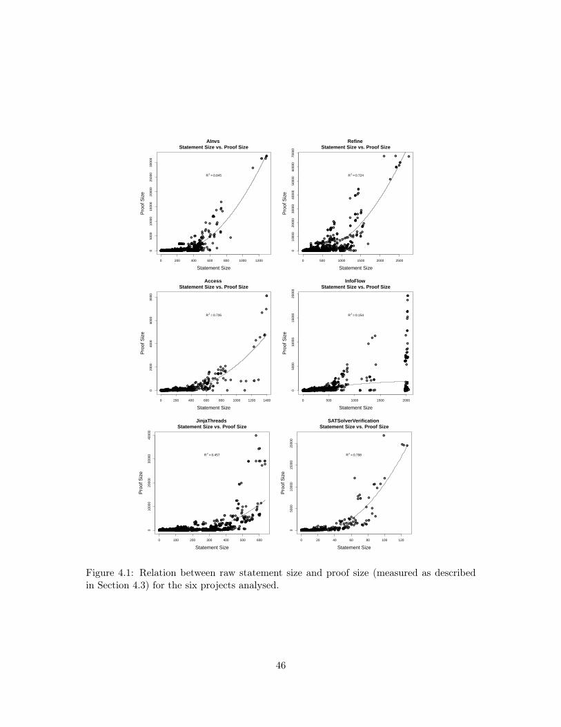
0 200 400 600 800 1000 1200

050

0010

000

1500

020

000

2500

030

000

AInvs Statement Size vs. Proof Size

Statement Size

Pro

of S

ize

R2 = 0.845

●●●● ●●

●●●

●●●

●

●

●

●●●

●

●

●

●

●●

●

● ● ● ●●● ●● ● ●●●

● ●

●

●●●● ●● ●● ● ●●

●

●●

● ●●●● ●● ●●● ●●●●●●● ●●●●

●●●● ●●●● ●

●●

●

●

●

●

●●● ●●

●

●

●●●●● ●●●●●● ●●●●● ●●●● ●●●●●● ●● ●●

●

●●●●

●

●

●●

●●

●

●

●

●

●

● ●●

●

●● ●

●●

●

●●

●●●●●●●●●●●●●●●●●●●●●●●● ●●●

●

●●

● ● ●●● ●● ●●

●

●

● ● ●●

●●

●●●●●●●●●

●

●

●

●

●

●

●●●

●●●●●●●●

●

●

●

●

●●●

●●●

●●● ●● ●●●●●●●●●●● ●●●●● ●●●● ●●● ●●●●●●● ●●

●

●●●

● ●●

●

●●● ●●●● ●●

●

●● ●●●

●

●

●

●●●

●● ●●●●●●

●

● ●●●

●

● ●

●●●● ●

●

●●●●●●● ●●●● ●●● ●●● ●●●● ●●●●● ●● ●●●●

●

●● ● ● ●●●●●● ● ●●

● ●● ●●● ●● ● ●●●

●

●●

●

● ●●●● ●● ●● ●●●● ● ● ●●●●●● ●●

●●

●●●

● ●●●

●

●

●● ●●●● ●● ●●●●● ● ●●●●●●●●●● ●●●●●

●●

●● ●●● ●●●●● ●●●●● ●●●● ●●●●● ●● ●●●●●●●●●●●●● ●●● ● ●●●

●

●●●●●● ●●●●●● ●●●●●

●● ●●● ● ●●

●

●● ●●● ●●●●● ●● ●●●●

●●● ●●● ●● ● ●● ●●●●

● ●● ●●● ●●● ●●●●●

●

●

●

●

●

●● ●●●● ●●●●●● ●●● ●●

●●

●●●●●● ●●●●●●●●●●● ●●●● ●●●●●

●

● ●●● ●● ●●●●●●● ●

●

● ●●

●

●●

●

● ●●●●●●●●●●●●●● ●● ●

●

●

●

●●●●●●● ● ●

●

●●●●●

●●●●●●●● ●●● ● ●

●● ●●●●● ●●●● ●●●

●

● ● ●● ●

●

●●● ●●●

● ● ●●●●●

●

●● ●● ●●●●●

●

●● ●● ●●●●●●●●●● ●●●● ●●●

●●● ●●●

● ●●●● ●●●●● ●● ●● ●●● ●●●●●●●●

●● ●●● ●● ● ●●●●●● ● ●●● ●● ●●●●● ●●●●● ●●●●●

●

●●●●●●●●●●●●●● ●●●●● ●●●● ● ●●●

●

●●●●●● ● ●

●

● ●●

●

●●●●●● ●● ● ●●● ●● ●●●●● ●

● ●

●●

● ●● ●●● ●●● ●●●

●

● ●●●●●●● ●

●

●

●●

●● ● ●●●●

●

●● ●●●●●● ●●● ●●●● ●●●●●●●

●

●● ●●●●●●●●●●● ●●

●●●●● ●●●●●●●●●●● ●● ●●●●● ●●●● ●●●● ●●●● ●● ●●● ●●●●●● ● ●

●

●●●

●

●●●● ●●●●●●●● ● ●● ●●● ●● ●

●●●

●●● ●●● ● ●●●●●●●● ●●●●

●●●●●●●● ●●● ●●●●●●●●● ●

●

●● ●

●

●● ●●● ● ●●●● ●●●●●● ●●●●●● ●●●●● ●●

●● ● ●●●

●● ●●

●

●●●● ●●● ●●●

●● ● ●●

●

●●● ●●●

●

●● ●●●●●●●● ●●● ●●●●●● ●●● ●

●

●●●●●●● ●●●●

● ●● ●●●●●●●●●●●●●●● ●● ● ●●●●●

●

●●● ●● ●●●●●●●●● ●●● ●●●● ●●●● ●●

●●

●

●●●●●● ●

●●●●●●●●● ●●●●●● ● ●●●●●●

●

●

●● ●●●●●●●●●●●●

●● ●●●● ●●● ●●●●●●●●● ●● ●●●●

●●●●● ●● ●●● ●● ●●● ●●

●

● ●●●●

●● ●

●

●●● ●●●●●

●

●●●

●●●●●●●●

●●●●● ●● ●●●●

●

●●● ●●

●●●

●●●

●●

●

●

● ●●●●●●●●●● ●

●

● ●●● ● ●●●●●●

● ●●●●●●●●●● ●●● ● ●●● ●● ●●● ●● ●●● ●● ●● ●●●●● ●●●●●●

●

● ●●●●● ●●●●●

●

●

●●

●●●●

● ●

●

●●●●●●●●●●●●●● ●● ●●●●

●●● ●● ● ●●●●●

●

●

● ●●●●● ●●●●● ●● ●● ●● ● ●●● ●● ● ●

●

● ●●●●●● ●●●●●● ●●● ● ●● ●●●

● ●●● ●●●● ●● ● ●●●● ●● ●●

●

●●●● ●● ●

●

●●●

●

●● ● ●

●

●●● ●●●●●● ●●● ●● ●●● ●

●●

●

●●

● ●

●

● ●●●●●●●●●●● ●●●●●●●●●●●●●●●●●●●●●●●●●●●●●●● ●●●● ● ●● ● ●●● ●●● ● ●●●●●●●●●●●●●

●●●●● ●●●●●●● ●● ●●●●●●●●●●●●●● ●●●●

●

●● ●●● ●●●●● ●●●●●●●●●●●●●●●●●●●● ●●●●●●●●●

●

●

●

●● ●●●●●●● ●●

●

●● ●●●●●●●●●●●● ● ●●●●● ●●● ●●●● ●● ● ●●● ●● ●●● ●● ● ●●●● ●●●●●● ●●●●●●●●

●●

●

●

●●● ● ●●● ●●● ●● ●●●●●●● ●●●●

●

● ●●●●●

●

●●●●●

●

●

● ●

●

●●● ●●●●●●●●●●●●●●●●●●●●●●●●●● ●●● ●●● ●●●

●●●

●●●

●● ●●● ●●●●●●●●●●● ●●● ●● ●

●●● ●

● ● ●●

●

●● ●●●●●●●●●●● ●●●●

●●●●

●

●●●●●●● ● ●●● ●●●● ●● ●● ●●●●●

●

● ●● ●●

●

●● ●●

●

● ●●●●●●●●● ●●●● ●●● ●●●●●● ●

●●●●●●●● ●●

●●

●●

●●●●

●● ●

●

● ●●● ●●● ● ●●●●●●●● ●●●●●

●

●●●

●●●●●

●

●

● ● ● ●●● ●●● ●●●● ●●● ●● ●●

● ● ●●

● ● ●●●●●● ● ●●● ●●●●●● ●●●●●●●●●●●●

●

●

●

●● ●●●● ●●●●

●●●●●●●●●●●●

●●

●●● ●●●●●●●●●● ●●●

●

●●●●

●●●●●

●

● ●●●●●● ●● ●●●●●●● ●●●●● ● ●●● ●● ●●● ●● ●●●

●

●● ● ●

●

●●●●●●●● ●● ●● ●● ●●●●●● ● ●●●● ●●●● ●●

●

●●● ●●●● ●

●

●●● ●●●●● ● ●● ●●●●●●●●● ●●●

●● ●●●● ●● ●●●●●●●●●●● ● ●●●● ●● ●● ●●●

●

●

●

● ●●●

●●●● ● ● ●●●●●●●●●●●●

●● ●●● ●●●● ●●● ●●●●●●●●●●●●● ●●● ●●

●●●

●●●

●● ● ●●●●● ●●●

●●

●

● ●

●

●●●

●●●●●●● ● ●●● ● ●●● ● ●●●●●●●●● ●●●●

●

● ●●● ● ●●

●●●● ●●●● ●●●● ●● ●●●●●●●● ● ●●● ●● ●●

●●●●● ●● ● ●●●

●

●●●● ●●●● ●●●● ● ● ●●● ●●●

●● ●

●

● ●●

● ●● ●● ●●●●

●●●

●

● ●●● ●●●●

●

●

● ●●●●●●●●●●●●●● ●●

●●●●●●● ● ●●●●●● ●● ●●●●● ●● ●●●● ●●● ●●● ● ● ●●●●●●

●●●●● ● ●●●●●●● ●●●●● ● ●●● ●●●●● ●●● ●●●

●●●●● ● ●

●

● ●

●●●●●●●●●● ●●● ●●●●●●●●●● ●●●●● ●

●●●● ●●● ●●●● ● ●●●● ●●●● ●● ●

●● ●●●● ●●● ●●● ●●● ●●●

●

●

● ●●●●●● ●●● ●●●●●● ●●● ●●●●●● ●●●●●●●●●●● ●●●● ●●

●● ● ●●●●●

●● ●●● ●

●

●●●

●●●●●●

●●●● ●● ● ● ●●

●●●●● ●●●●●●●●●●●● ●● ●●●●● ● ●●●● ● ●● ●● ●●●●●●●

●

●●●● ●●●●●●●

●●●● ●

●

●

●

●● ●● ●●●●●●●● ●● ●

●●

●●●●● ●●●● ●●●●● ●●

●

● ● ●●●●● ●●●●● ●

●

●●

●●●

●● ●●●●●●●● ● ●●● ●●●

●

●

●

●●● ●●●●●●●●●●●

●● ●●●

●●●

●

●●●●●●●●●●●●

●

●●●●●

●

●

●

●●● ●

●

●●●●●●● ●●●●●● ●● ●

●● ●●●●●●●●

●●

●●●●●●● ● ●●●

●

●

●

●●●

●● ●●●●● ● ●●●●●●● ●● ●● ●● ● ●●● ●● ●●●● ●●● ●

●● ●●● ●● ●●●●●● ● ●●●●●●

●●●●●●●●●●● ●●●●● ● ●● ● ●

●

● ●●●●●● ●● ●●●●

●

●

●●●●●●●●●●●● ●

●●

●●●● ●

●

●●●●●● ●

●●●●●●●

●●● ● ●● ●●

●●

● ●●

●●●● ●●●

●

●

●● ●●●● ●●●●●● ●●●●

●●

●●●● ●●●● ●● ●● ●● ●

●● ●●●

●● ●●● ●●●●●●●●●●●●●●●●●●●●●●● ●● ●●● ●● ●●●● ●●● ●● ●

●● ●●

●

●

●● ●●●●● ●●

●

●●●● ● ●●●●●● ●● ●●● ●●● ●●

●●●●● ●

●

● ●●● ●●●

● ●●●●●

● ●● ●●●●●

●● ●●●●

●●● ●●● ●●●

●

●●●●●●●

●

●● ●●●● ● ●●●●● ●●●●●●●● ●●● ● ●●● ●●●●●

● ●● ●● ●●●●● ●●

●

●●●●●● ●●●● ●●●●● ●● ●●● ●●●●●●●●●●● ●●●●●

●●

●●● ●●●● ●● ●●

●● ●●

●●●●●●●●●●

●●●

●●●●●

●

●

●●●●●●● ●●● ●●●●●●●●●● ●● ●

●

●●●●● ●●● ●● ●●● ●

●●●● ●●●●●● ● ●

●●●●●

●●

●● ●●● ●

●

●●● ●●●● ●●●●●●●●●

●●●● ●●

●●●●●● ●●●●●

●● ●●● ●●● ●●●● ●●●●● ●● ●●●

●

● ●●●●●●

●●●

●

●

● ●●●●●● ● ●●●

●●● ●●● ●●● ● ● ●●●●●●

●

● ●● ●●

●

●● ●● ●●●●●●●●●● ●●●

●●●●

●●●● ● ●●●● ●●● ●

●●

● ●●●● ●●●●● ●●● ●●●● ●● ●●●● ● ●●● ●●●●●●● ●●

● ●● ●●●●● ● ●●●●●●●●●●●●● ●●● ●

●●●

●

● ●●● ●● ●● ●● ●●●●●

●

●

●

●● ●●●

●●●●●●●●●●●● ●●

●

●●●● ●●●●●●●● ● ●●●●

●●● ●●●● ●●

●●●●●● ●

●

●● ●●●

●

●●●●●●●●●●●●● ●●●● ●

●●●●

●

●

●●● ●●● ●●●

●●●● ●●●●●●●●●● ●

●●●● ●●

●●●● ●●

●

●●● ●●●● ●●● ●●●●●●●●●●●● ●●●●●●●

●●●

●●●● ● ● ●●●●●●●●● ●●

●●●●

●●●●●●●●●● ●● ●●●●●●●●●●●●●●● ●●● ●●●●●●● ●●

●

●●●●●●●● ● ●●

●

●● ●

●●●●● ●●●●

●●

●● ●

●●

●●

●

●●

● ●●

●●●●

●● ●●●●●

●●● ●●

●● ●●●●

●

●● ●●●● ● ●●●●●

●●●●

●●●●

●●

●

●

● ●●● ● ●● ●●

● ● ●●●●●● ●●

●

●

●●

●●

● ●●●● ●●● ●●● ● ●●● ●●●

●

●●●●●● ● ●●●●●

●● ●●●

●

●●● ●●●

●

● ●● ●●●

●

●

●

●● ●●● ●●●●●●● ●●

●

●●●

0 500 1000 1500 2000 2500

010

000

2000

030

000

4000

050

000

6000

070

000

Refine Statement Size vs. Proof Size

Statement Size

Pro

of S

ize

R2 = 0.724

●●●● ●● ●●●●●●●● ●●●●● ● ●●● ●●● ●●●● ●● ● ● ●●●● ●●●●

●● ● ●● ● ●●● ●●● ●● ● ●● ● ● ●●● ●● ●● ●●● ●● ●●

●●● ●●●● ● ●●● ●●●●● ●● ●●●●●

●● ●●● ●●●

●

●●● ●● ●● ●●●● ●●

●

●●

●●●●

●

● ●●● ●●● ●● ●●

●

●●● ●● ●● ●● ●

●

●● ● ●●

●● ●● ●●● ●● ● ●●● ●●●●●

● ●●●●

● ●● ● ●● ● ● ●● ● ●

●

● ● ●● ● ●●● ●●● ●●● ●●●● ●●● ● ●● ●●●●

● ●●

●●

●

●●

● ● ●●● ●● ●

●

●●●● ● ●●●

●

●

●

●

●

●●● ●● ● ●●●●● ●●● ●●●

●●●●

●●

●

●

● ●●●● ●●

●

●●●●

●

●

●

●

●

●

●

●● ●●● ● ●●● ●

●● ●●●●●● ●

●

●

●

●●

●

●●●

●

●

●

●●

●●

●

●

●●●

●

●●●● ●●●●●● ●

●

● ●

●

●

●●●●

●

●

●

●● ●

●

●●●● ● ● ●●● ●

●●

●

●

●

●●● ●● ●

●

●

●

●●● ●●● ●●● ●

●●●●●●

●

●

●

●

●

●

●

●

●●

●

●

●

●●● ●●●● ●●●● ● ●

●●●●● ● ●

●

●● ●

●●

●

●● ●

●● ●●

●●●

●

●

● ●●●●● ●●

●●

●

●

●

●●●

●

●

●● ●

●

●●●● ● ●●●● ●

●●

●● ●●

●●

●●

●●

●

●

●●● ●

● ●●

●

●●●

●●

●

●● ● ●●●●

●

●

●

●

●

●

●

●●

●

●●●● ●●

●

●●

●

●● ●● ●●●● ● ● ●

●

●

●

●●●

●

●● ●●●●●●●

●

●●

●●●●

●●● ●●●●●●● ●

●

●

●

●

●

●● ●

●● ●● ●● ● ●● ●● ●●●●●

●●● ●●● ●● ●●●●●

●

●●

●●

●●●●

●●

●●

●

● ●●●●●

●● ●●●

●

●

●●

●●

●

●●

●● ●●

●

●●

● ●●

●●

●

●●

●● ● ●

●

●

●●● ● ●

●●● ● ●●

●●●●● ●

●●

●●

●● ●●

●●

●● ● ●●● ●● ●●● ● ●●●●●● ●

0 200 400 600 800 1000 1200 1400

020

0040

0060

0080

00

Access Statement Size vs. Proof Size

Statement Size

Pro

of S

ize

R2 = 0.735

●●●●●●●●● ●●

●●●●● ●●●●● ●●●●● ●● ●● ●●●●●● ●●●●●●● ● ●●●● ●●●●●●●●●●●●● ● ●●●● ●●●●● ●●● ●● ●●●● ●●●●● ●●● ●●●●● ●●●●●●●●● ●●● ●●● ●●●● ●●● ●● ●● ●●●● ●●● ●● ●●● ●●● ●● ●●●●●●●●●●●●● ●●●● ●●●● ● ●●●

●

●● ●●● ●● ●●● ●● ●●●●●●●●●●

●●●●●●●●● ● ● ●● ●● ●●● ●●●●

● ●

●●

●●● ●●● ●●● ●●●●●●●● ●●

●

●● ●● ● ●●●● ●●●● ●●●●● ●● ●●● ●

● ●●●●● ●● ●

●●●

●●● ●●●●●● ●●● ●● ●● ●●●

●

●

●

●●

●

●●● ● ●●● ●●●● ●● ●●

●

● ●●●●●●● ●● ●●● ●●●●●● ●● ● ●●● ● ●● ●●

●

●●

●

●

● ●●● ●●

●●●●●●●●

●

●

●

●

●●●●● ●●●● ●●●● ● ●●● ●●●

●● ●●● ●●

●●

●

●

●

●●● ●● ●●●●● ●● ●●● ●●●

●

●

●

●

●

● ●● ● ●●●●●● ●●● ●●●

●● ●●●●

●

●●● ●●

●●●●● ●● ●●

●

●●●●●

●

●

● ●● ●● ●

●

●● ●● ●● ●

●

●● ●● ●●

●●● ●●●

● ●●

● ●●●●●

●●

●

●

●● ● ●●●●● ●●●●

● ●●●●● ● ●●● ●

●● ● ●●●

●●●●●● ●●●

●●● ●●●●

●

●●● ● ●● ●●●● ●● ●● ●

●

●●●● ●●● ● ●●●●●●● ● ●● ● ●●●● ● ●

●●

●● ●●●●● ● ●●

●●

●

●

●● ● ●●

●●●● ●●●

●

●● ● ●

●

●● ●●● ●●● ●●●●

●

●●● ●

●

● ●●●●●

●●

●

● ● ● ●

●

●

●

● ●●● ●●● ●

●●●

● ●●

●

●●● ● ● ●●●● ●●●●

● ●●●●● ● ●● ●●

● ●●●

●

● ●

●

●●

●●●

●

●

●● ●●● ●●●

● ●● ●●

●

●

●

●

● ● ●

●

●● ●●

● ● ●●● ●●●●● ●●● ●● ●● ●●●● ● ●●●● ●●●

●● ●●●

●

●● ●● ●●●

●●●● ●●●

●

●●

● ●●●●

●● ●● ●●●●●

● ● ●●●

●●● ● ● ●●● ●

●

●●●●

●

●●●● ●●●●

●●●

● ●●

●

●●

●●

●● ●●● ● ●● ●●● ●●●● ●

●

●

●

● ●●● ● ●● ●●● ●● ●●●●●● ● ●●●● ●

● ●●●

●

● ●●

●

● ● ● ●● ●

●●●● ● ●● ● ●●

●

●●●●

● ● ● ●

●

●●●●●●● ● ●● ●●●●

●

●

● ● ●●● ●

●

●● ●●● ●●●● ●●●

●●●

●

● ●●●●●●●● ●●●●

●

●

● ● ●●● ●●● ●●●● ●●●

●●

●

●

●● ●●●●

● ●●

●

●●●● ●●● ●● ●●●●● ● ●●●

●

●

●

●●●● ● ●●●● ●● ●●●●

●●

●●● ●

●●●●

●

●● ●●● ● ●● ●● ●●●●

●

●●

●

●●●● ●●●●● ● ●

●●

●

●●●●●●

●

●●● ●●●

●

●●● ● ●●●●

●

●●● ●●●●● ●●●●●●●

●

● ● ●●●●●

●●

●

●●●● ● ● ●● ●●● ●●●●● ●● ● ●

●

●

●● ●●● ●●●●●

●●

● ●●●● ●

●●●●●

●● ●

●●

●

●

●●●●

● ● ●●

●

● ●● ●● ●●

●

●●● ●●●●●

●

●●●● ● ● ●

●

●●●

● ●●●●● ●● ● ●●

● ●

●●

●●●● ●●

●

●●●

●●

●

●

●●

● ●●● ●●

●●●● ●●●● ●●●

●

●●

●

●●●●

●

●●●

● ●●●● ●● ●●●●● ● ●●● ●●●●●● ●●●●●

●● ●●●

●

●

●

●

●

●

● ● ●● ●●●●●●●●●●●●●●●

●

●

●●●

●

● ●●●●

●

●●

●

●●●●

●

●●●

● ●●● ●●●●● ● ●●●●●●●●

●

●

●●●

●

●●●●●

● ●●● ●● ●●

●

●

●

●●●●●

●● ●● ●● ●

●

●●●

●

●●●● ●●● ●● ●● ●●● ●● ●●

●

● ●●●●●●

● ●●● ●

●

● ●

●

●●● ●● ●

●

●

●●●●

●

●● ●● ●●

●

●● ●

●

●● ●●●

● ●●

●

● ●

●

●●● ● ●●●● ● ●●●

●●●

●

●

●

●●●

●

●●●

●●

●

●●●●

●

●●

●

●●●●● ●●

●

●

●

●

●●●

●

●● ●●● ●● ●

●

●

●●

●

● ●●●●● ●●● ●

●

●● ●

●

●

●●

● ●●●●

●

●●

●

●

●●

●

●

●

●

●

●

●

●

●

●

●● ●

●

●

●

●

●

●

●

●

●

●●

●

●●

●

●●

●

●● ●● ●●

●

●

●

●

●●●● ●

●

●

●

●● ●●●

●

●

●

●●

●●●●

●●●

●●●●●●

●

●●●

●●

●

●●

●

●●●●

0 500 1000 1500 2000

050

0010

000

1500

020

000

InfoFlow Statement Size vs. Proof Size

Statement Size

Pro

of S

ize

R2 = 0.154

●● ● ●●●●●●●● ●●●●●●●●● ●● ●● ●●●●●● ●●●●●●●●●●● ●●● ● ●● ●●●●●● ●●●●●●●●●●●●●●●●●● ●●●●●●● ●●●●● ●●●●●●●●● ●●●

●

●●●●●●●●● ●●●● ● ● ●●●●●●● ● ●●●● ●●●● ●●●●●●●●●●● ●●●●●●●●● ● ●●●●●●●●●● ●●●● ●● ●●● ●●●●● ●●●● ●● ●●●●●●●●●●●● ● ●●● ●●● ●●●●●●●●● ●●●●●●●●●●●●●●●●●●● ●● ●● ●● ● ●●●● ●●● ●●●●● ●●●●●● ●●●●●● ●

●

●●●●●●●●●●●●●●● ●●●●●● ●●●●● ●●

●

●●●● ●●● ●●●●●● ●●●● ●●

●● ●●●●●●● ●●● ● ●● ●●●

●●

●●●●●●●●●●●● ●●●●●●● ●● ●●●●●●●●●●●●●●● ●●●●● ●●●●●●●●●●● ●●● ●●●●●●● ●● ●●●

●

●●●● ●●●● ●● ●●●●●●●●●●●●●● ●●●● ●●●●●●●●●●●●

●●●●

●

●● ● ●●●●●●●●●●●●●●● ●● ●●

●●●●●●● ● ●●●●●● ●●●●● ●●● ●●●●●●●● ● ●●● ● ●● ●●●●●●●●●● ● ●●●●●●●●●●●●●●●●● ●●

●●

●● ●●● ●●●●●●●●● ●●●●●●●●●●●●●●●●● ●● ●●●●●●●●● ●● ●●

●

●●●●● ●● ●●●●●●● ●● ●●●●●●●●●● ●●●● ● ●●●●● ●●● ●●●●●●●●●●● ● ●●●●●●●● ●●

● ●●●●● ●●

●

●●●●●●● ●●●●●●●● ●●●●●● ●●

●●● ●● ●●●●●●●●● ●●●●●●● ●●

●●●●●●●●● ●●●●●● ●●● ●●●● ●●●●● ●●●●●●●● ● ●●●●●●●

● ●●●●●● ●● ●●●●

●

●●●● ●●●●●●● ● ●● ●●●

● ●●●●●●●

●●●●●●●● ●●●●● ●●●●●●●●●● ●

●

●●●●● ●● ●●●●●●● ●●● ●●● ●●●●●●● ●●●●●●●●●●● ●●●●●●● ●●●●●●● ● ●● ●●● ●● ●●●

●

●●●●●●●●●●●● ●● ●● ●●● ●●● ●● ●●●● ●● ●●●●●●● ●●●●●●

●●●●●●●●●●● ● ●● ●● ●● ●●●●●●● ●●●●●●●●●●●●●●● ●● ●● ●● ●●●● ●●● ●● ●●●● ●● ●●●● ●●●●●●●●●●● ●●●●●●● ● ●● ● ●●●● ●●●●

●●●●●●● ● ●●●

●

●

●●●●●●● ●● ●●●●●●●●●●●

●

● ● ●●●●●●● ●●●●● ●● ●●●●●●●●●●●●● ●●● ●●● ●● ●● ●

●

● ● ●●●● ● ●● ●● ● ●●●●●● ●●●●● ●●●●●●●● ●●●●●● ●●● ●●●

●●●●●●●●●●● ●●●●● ●●● ●● ●●●●●●●●●●●●●●●●●● ●●● ●●●●●● ●●●●●● ● ●

●●●● ●●● ●● ● ●●●●●●●●●●●●●●●●●● ●● ●●● ●● ●● ●●●● ●●●●●● ●●● ●●●●●● ●●●●●●●●●●●●●●●●● ●●● ● ●●● ●●● ●●●●●●●●●●●●● ● ●●●●●●●●●● ●●● ●●●●●● ●●●

●●●●●●●●●●●●●● ●● ●●●●●● ●●●●●●●●●●●●●●●●●●●●●●●●●●●●●●●●●●●●●●●●●●●●●●●●●●●●●●●● ●●●●●● ●●●

● ● ● ●●● ●●● ●●● ●●● ●●●● ●● ●●● ●●●●●●●

●

● ●●● ● ●●●●●● ● ●●● ● ●●●●

●●

●

●● ●● ●●●

●●●●●●●●●●●● ●●●●● ●●●●● ●● ●●●●●● ●●●●●●●●●● ●● ●●●●●●●●●●●●●●●●● ● ●●●●● ●●●●●●● ●●●●●● ●●●● ●● ●● ●●

● ●●●●● ●●

●

●● ●●

●

●● ● ●● ●●● ●

●

●●●●●●● ●●●●

●● ●●● ●●●● ●●●●●●●● ●●●●●● ●●● ●●●●●●●●● ●●● ●● ● ●●●●●●● ●●●●●●●●●●●●● ● ●●●●●●●● ● ●●●●● ●●●● ●●●● ●●●● ●●●●●

●●●●●●● ● ●●●●●●● ●●

●●●●● ● ●●●● ●●●●● ● ●● ●●●●●●●● ● ●● ●● ●●●●●● ●●● ●●● ●●●●●●●●●●●●●●●●●●●●●● ●● ●●●●●●●●●●●●●●●●●●●●●●●●●●●●●●●●● ● ●●●●●●● ●●●●●●

●

●●●●●●●●●●● ●●● ●●● ●●●●

●● ●●● ●●● ●● ●●● ●● ● ●●●● ●●●● ●●●●●●●●●●● ●● ●● ●●●●● ●●●●●●●

●

● ●●●●●●●●●●●●●●●●●●●●●●●●●●●●●●●●●●●●●●●●● ●●●●●● ● ●●●●●●● ●●● ●●●●●● ●●●●●●●●● ●●●●●●●●●●●● ●●●●●● ●● ●●●

●

●●●●●●●● ●●●●● ●●● ● ●●●●●● ●●● ● ●●●● ●●●●●● ●● ●●●● ● ●●●●●● ●●●●●●● ● ●●● ●●●● ●● ●●●●●●● ●● ●●●●●●●

●●●●●●●●●●● ●● ●●●●●●●●● ●●●●●● ●●● ●●●●● ●●●●●●●●●● ● ●●●● ●● ●●●●●●● ●● ●

●●●●●●● ●●●●● ●●●●●●●●●●●●●●● ●●● ●●●●●● ● ●●●● ●●

●

●●●● ●●●● ●●● ● ● ●●● ●●●●●●● ●●●●●●●●●●●●●●●●●●●● ●● ●●●●●●●●●●●●●●● ●●●●●● ●●●●●●●●●● ●●●●●●●●●●●● ●●● ●● ●●●●

●

●●●● ●●●

●●

● ●●●

●●

● ● ● ●●●●●●●●●●●●●●●●●●●●●●●●●●●●●●●●●●●●●●●●●●●●●●●●●●●●●●●●●●●●●●●●●●●●●●●●●●●●●●●●●●●●●●●●●●●●●●●●● ● ●●●●●●●● ●●●

●

● ●●●● ●●●● ●●●●●●●●●●●●●●●●●●●●● ●●●●●●● ●●●● ●●●●●●●●●●●●●●●●●●●●●●●●●●●● ●●●●●● ●●●●●●●●●●●●● ● ●●●●● ● ● ●● ●● ● ●● ●●●●

●

●●● ●●● ●●

●●●● ●●●●● ●●● ●●● ●●● ●●

●

●● ●●●● ●●●● ●●● ●●●●●●●●●●●●●● ●●●● ●●●●●●●●●●●●●●●●●●●●●●●●●● ●● ●●● ●●●●● ●●●●●●●●●●●●●●●●● ●●●●

●

●●●●●●●●●●●●●●●● ●●● ●●●●●●●●● ●●●●●●●●● ●●●

●

●●

●

● ●

●●

●●● ●● ●● ● ●●● ●●●●●●● ●●● ●● ●●● ●●● ●●●●●●● ●●●●● ●●●●● ●

●

●● ●●●●●●●●●● ●●●●●●●●●●●●●●●●●●●●●●●●●●●●●●●●●●●●●●● ●●●●●●●●●●●●●●●●● ● ●●●●●●●●●●●●●●● ●●●●●●●●●●●●● ●●● ●●●● ●

●● ●●●●●● ●●●●●● ●

●●

●●

●●●●●● ●●●● ●● ●●●●●● ● ●● ●●● ●●● ●●●● ●●● ●●

●

●●● ●●●●●●●●●●●●●●

●●

●●●●●●●●●●●●●●●●●● ● ●●●●●●●● ●●●●●●●●●●

●● ●●●●

●● ●●●●●●●● ●●● ●●● ●●●

●

● ●●● ● ●●●●●●●●●●●●●●●●●●●●●●● ●● ●●● ●●●●● ●● ●●● ●●

●

●● ●●●● ●●●●●●

●

●

●●● ●●●● ● ●●●●●●●●●●●●●●●● ●●●●● ●●●●●● ●●●● ● ●●●●● ●●●

●●●● ●●●●● ●●●●●●● ●● ●

●

●●●●● ●●● ●●●●●●●●●●●●●●●●●●●●●●● ●● ●

●

● ●●

●●●●●●

●

● ●●●● ● ● ● ●●

●●● ●●●●●● ● ●●●● ●●●●●●●●●●●● ● ●●●● ●●●●●●● ●

●●●●● ●●●●● ● ●● ●●● ● ●●● ●●●●●●●●●●●●●● ●●● ●●● ●●

●●●● ●●●●●●● ●● ●●●

●

●●●●●● ●

●

●●●●

●●

●

●●● ●●●●●●● ●● ●●●●●●●●● ● ●●● ●●●●● ● ● ●●●●● ●●●● ●●●●●●●● ● ●●

●

●

● ●●● ●● ●●●●● ●●●● ● ●●●●●● ●●●●●● ●

● ●●

● ●

●●● ●●●●●●● ●●● ●● ●●

●

●●●●●

●

● ●●●

●●

●● ●●●

●●● ● ●●●●●● ●●●●● ●●●● ●●●●●● ● ●● ● ●●● ●●●●● ●●●●●● ●●●●● ● ●●● ●●●●●●●●●●●●●●●●●

●● ●● ●●●

●●●

●●●●● ●●

● ●● ●●●

●

●

●

●

●●●●●●● ● ●●●●●●●●● ●●●●●●● ●● ●●●● ● ●●●● ●●● ● ●● ●● ●●●●● ●●●●●●●● ●●

●

●●

●

● ●●●●● ●● ●●●●

● ●●●●●●●●●●●●●●●●●●●●●●●●●●●●●●●●●●● ●

●

●●●●●● ●●

● ●●●●●●●●● ● ●● ●

●●●●

●●●● ●●● ●

●

● ● ●●●●● ●●●●●●●●● ●●●●●●●●●●●● ●●●●● ● ●● ●●● ●● ●●●●● ●● ●●●●

● ●●● ●●●●●●●●● ●●●●● ●● ● ●●●●

●

●●●●● ●●● ●

●

●

●

● ●●●●●●● ●●●● ●●● ●● ●●● ● ●●●●●●●●● ●● ●●

●●●●● ●●

●●●●●● ●●●●●●●

●●●● ● ●●●●

● ●●●●●●●●●●●●●●●●●● ●●●●●●●●●●●●●●●●●●● ●●●● ●●● ● ●●●●●●● ●●●●●●●●● ●●●● ●●● ●●●●●●●● ●

●

●● ●●● ●●● ●●●

●● ●● ●●●●● ●●● ●●

● ●●●●● ●●●●●●●●●●●●●●●●●●●●●●●●●●●●●●●●●●●●●●●●●●●●●●●●●●●●●●●●●●●● ●●●●●●●●●●●●●●●●●●●●●●●●●●●●●●●●●●●●●●●●●●●●●●●●●●●●●●●●●●●●●●● ●●

●

●● ●●●●●●●● ●●● ●●● ●●● ●● ●●

●●●●

●

● ●●

●

●●●● ●

●

● ●●●●●●●● ●●

●●●●● ●●●●●●●

●

●●

● ●●

●

● ●●●●● ●● ●● ●●●● ●● ●●● ●● ●●●●●●●●●●●●●●● ●

●

●●

●

●

● ●● ●● ●

●●

●

●●●●

●●●

● ●●● ●●●

●

●●●

●

● ●●●

●

●

●

●

●●● ●● ●●●●● ●●

●

●●●●● ●● ●● ●●●●●●●●●●●●●●●●●●●●●●●●●●●●●●●●●●●●●●●●●●●●●●●●●●●●●●●● ●●●●●●●●●●●● ●

●

●● ●● ●●●●

●

●● ● ●● ●●

●

●●●●●●●● ●●●●● ●●●●

●●

●●

●● ● ● ●●● ●●●

●●●● ●●●● ●●● ●

●●

● ●● ● ●● ●●● ●●●

●●●●●●●●●●●●●●●●●●●●●●●●●●●●●●●●●●●●●●●●●●●●●●●●●●●●●●●●●● ●●● ●● ●●

●

● ●●●●●●●●●●●●● ●

●

●

●●●●● ●●●●●●

●●

●

●●

●●●●●●● ●●●●●

●

●

●●●

●

●

● ●●● ● ●●● ●● ●●●●●

●●● ● ●●● ●

●

●●●

● ●●

●

●

●● ●●

●

●●●●●●●●●●●●●●● ●●●●●●●●●● ●●

●

●

●● ●●

●

●

●

●●● ●

●●● ●●●●●

●

●●●●●●●●●●●● ●●● ●●●●● ●●● ●

●●

● ● ●

●

●●●●

●

● ●● ●●

●● ●

●●

●●●●●●●●●●

●

● ●●●●

●●●● ● ●●●●●●●●●●●●●●●●●●●●●●●●●●●●● ●●●● ●● ●

●

●●● ● ●●

●● ●●●● ● ●● ● ●●

● ●●

●●● ●●●●●●●●●●● ● ●●●

●●●●

●●

●● ●● ●● ● ●●● ●●●●●● ● ●●● ●●● ● ●●●● ●● ●●● ●●●●● ●●●●●●●●

●●

●

●

●

● ● ●● ●●●

●

●●●● ● ●● ●● ●●● ●●

●●● ●●●●●●● ●●● ●●●●●●●●●●●● ● ●●

●● ●●●●●

●● ●●

●●●●●●●● ● ●●●●●●●●●●

●

●

●●●

●

●●

●● ●

●

●●●●●● ●● ●●●●● ● ●● ●●● ●●●●●●●●●●●●●●

●●●● ●● ●● ●

●

●

●●● ●

●

● ●●

●

●

●

●

●● ●

●●

●●●●

● ●●●● ●●●●●●●●

●

●●●● ● ●●● ●

●

●● ● ● ●●● ●

●

●●●● ● ●●●●● ●●

●●●

●●● ● ●●●●

●

●●●●

●●

●●●●●●● ●●●●●

●●●●●● ●●●● ●

●●● ●

● ●●●●●●●●●●● ●● ● ●

●

●

●

●

●●●●● ● ●●● ●●●●●●●● ●●

●●

● ●

●

●●●●●

● ●

●●●●●●●

● ●● ●●● ●● ●

●

● ●●

●

●●●●●

●●

●●●

●●●

● ●● ● ● ●●●●

●

● ●●●●●●●

●●●

●

●

●

● ●●●

●

●●●●● ● ●●●●●● ●●●●●●●● ●● ●● ●●● ●●●●●●●●

●

●

●

●

●●●●

●

●●●● ●●● ●

●

●

●

●●● ●

● ● ● ●●●●●●● ●●● ●

●●● ●

●

●●●● ●

●

●●● ● ●●● ●● ●● ●

●●

● ● ●●●●● ●●●

●

● ●●●●●●

● ●●

●●

●●

●●●●●●●●● ●●●● ●●●● ●●●●

0 100 200 300 400 500 600

010

000

2000

030

000

4000

0

JinjaThreads Statement Size vs. Proof Size

Statement Size

Pro

of S

ize

R2 = 0.457

● ●●● ●● ●● ●● ●● ●●●●●●● ●●● ●●● ●●●●●●●● ●●●●● ●●●●●●●● ●● ● ●●●● ●●●●●●●●● ● ● ● ●●●●●●●● ●● ●● ●●●●

●●● ●●●●● ● ●●●●● ● ●● ●●● ●●●●●●● ●●● ●● ● ●●●●●●● ●● ● ●●● ●●●●●

●

●● ● ●●●● ●● ● ●●● ●●●●

●

● ●●●●●● ●●

●●● ●●●

●● ●●●● ●●●●●●

●

●● ●●● ●●●●●

●●●●●

●●●●●●●●●● ●●● ●●

●

●

●

●●● ●● ●●● ●●● ●●

●●

●●● ● ●● ●●●●●●

● ●

●●●● ●● ●

●

●

●●

●

●● ●●●●● ● ●●●●●● ●● ●●●

● ●●

● ●●● ● ●●●

●●

●●●● ● ●

●

●●●●●

●

●

●

● ●

●

●● ●● ●●

●

● ● ●

●

● ●●

●

● ●

●

●●

●

●●

● ●● ●● ●●

●

●

●

● ●●● ●●●

●

●●●

●●● ●

●

●

●

● ●●● ●●

● ●

●

●

●●●●

●●●● ●●

●

●

● ●●●

●

● ●● ●

●

●● ●

●

● ●●●

●

● ● ●● ●

●

●●

●

● ●●●●

●●

●●

●●

●●●●

●

●

●

●●

●●●

●

●

●●

● ●●

●

●

●●

●

●

●●

●● ● ●

●

●●●●●

●

●

●

●

● ●●●

●

● ●●● ● ●

●●

●

● ●

●●

●

●

●●● ● ●

0 20 40 60 80 100 120

050

0010

000

1500

020

000

SATSolverVerification Statement Size vs. Proof Size

Statement Size

Pro

of S

ize

R2 = 0.798

Figure 4.1: Relation between raw statement size and proof size (measured as describedin Section 4.3) for the six projects analysed.

46

●

●

●

●

●

●

●

●

● ●

●●●

●

●●●● ●●

● ●

●● ●●●

●

● ●●●● ●

●

●

●●

●

●

●

●

●

●

●●●

●●●● ●● ●●

●

●●●●● ●●● ●

●●●

●●●●●●●●●●●

●

● ●●●● ●●● ●●● ●●●●

●

●

●

● ●

●

●

●

●● ●●●●●●●●●●● ●●●●● ●●●● ●●●●●●●● ● ●●●

●

●●● ●●●●

●

●●●

●

●●

●

●●●●●

●●●● ●● ●● ●●● ●●●●●●●● ●●● ●●● ●●●●●● ●●● ●●●

●

●●●●●●●●●

● ●●

●

●●●● ●● ●●●● ●●●●●●●●●●●● ●●● ●●●● ●●●● ●●●●●●● ● ●●

●

● ●●●●●●●●●●● ●● ● ●●●●●

●

● ● ●●●

●●●

●

●●●●●

●

●●●●● ● ●● ● ●●●●●●●●●●●● ●● ●●●

●

●● ●● ●●●● ●●●●●● ●● ●

●

●

●●●●●

● ●

●

●●●●●● ●● ●●●●

●

● ●● ●●●●●●●●

● ●●●●●●●●

●

●●● ●●●●●

●●

●●●●●● ●

●

●● ●●● ●●● ●● ●●●●●● ●● ●●●●●●●●● ●● ●●●●●●●●●● ●●●● ●

●●●●●

●

● ●● ●● ●●●● ●●●

●●● ●

●● ●●

●

●

●●●● ●● ●●● ● ●

●

●

●

●●●●●●●●

●

●

●

●●● ● ●●● ●●● ●●●●●●●●●●● ●● ● ●●● ●●●●● ●●● ●●● ●●

●

●● ●●● ●●●●●● ●●●●●

● ●●● ●● ●●●●

●

●●

●●●●●●● ●●● ●

●●●● ●●●●● ●●● ● ●●●

●

●

●

●●●● ●●●●●●● ●●●● ●●●●●●●●●●

●

● ●

●

●●● ●●●● ●●● ●●● ●●● ●● ●●●●●●● ● ●●●

●

●

●

●●

●

●●● ●●●● ●●●● ●●● ●●●●●

●

●● ●●● ●●●●● ●●●● ●●

●

●●●● ● ●●● ● ●● ●●●

●

●●●●●●●●●●●●● ●

●

● ●●● ●● ●● ●●● ●●●● ●●

●

●

●●●●

●●

● ●● ●●●●●●●●●● ●●●●●●● ●●● ● ●

●

●● ●

●

● ●●● ●● ●●● ●●●● ●●●● ●● ●●●● ●●●● ● ●● ●●●● ●●

●

●●●●●● ●●●● ●●●● ●●●● ●● ●●● ●●●●●● ●●● ●●●●● ●●●●● ●●

●

●●

●

● ●●●●●●●● ●●

●●

●

●

●●●●●

●

●● ● ●● ●●●

●

● ●●●●● ●●●●●●●●

●

●

●

● ●●●●● ●●●●●●●●●●●●●●●●●●●●●●●● ●● ●●●●● ●● ●●

●

● ● ●●●●

●

●

●

●●●●●●●● ●●● ●●●●●●●●●● ●●●● ●●●●●● ●●●●● ●●●● ●● ●●●●

●

●● ●●●● ●

●

●●● ●●●●●●●●●●

●●●●●● ●●● ●●●●●●●●●●●●● ●●● ●●●● ●● ●●●● ●●● ●●●●● ●●●● ●● ●● ●●●●●● ●●●●● ●

●●●● ●●●●●●● ●● ● ●●●●●●● ●● ●●● ● ●●●●●●● ● ●● ●

●

●

●●● ●●●●● ● ●●

●●● ●● ● ●● ●●●● ●

●

●●●●●●● ●●● ●● ●●●● ●●● ●●●● ●●● ●●● ●●●●●●●●●

●

●●●●● ●●

●

● ●●● ●●

●

● ●● ●●

●

●●●●●●●●● ●● ●●● ●● ● ●

●●●●● ●●●●●●●●●●● ●●●● ●●●●●

●

●●●●● ●●●●●●● ●●● ●●●● ●●●● ●●●●●

●

●

●●

●

●●●●●●● ●●●● ●●●●● ●● ●● ●● ●●●●●●● ●●

●

●●●

● ●●● ●

●

●●

●● ●● ●● ●●●●●● ● ●●

●

●● ●● ●●●

●● ●● ●● ●●●●●●● ●●

●

●●●●●●●●●●●●● ●●● ●●●● ●●●●●● ●●●● ●● ●●● ●●●●● ●●●●●● ●●●●●●● ●●● ●●

●

● ●● ●●●●●

●

● ●●●●●●●●● ●●● ●● ●●● ●●● ●

●

●● ●●● ●● ●● ●●●

●●●

●●

●

●

●

●●

●● ●●● ●●●●●●

●● ●

●

● ●●● ●●●

●

●●● ●●● ●●●●●●●

● ●●●●

●

●

●●●●●●●●●●●●●●●

●

●●●● ●●

●

●

●●● ● ●●●●●●●●● ● ●●●●● ●●●●● ●●●● ● ●● ●●●● ●●● ●● ●●●

●

●●● ●●

●

●●

●

●●●● ●●●●●

●

●●● ●● ●●●●● ●●●●● ● ●● ●●●●●● ●● ●●●●● ●●● ●●●●● ●● ●●●● ●●●● ●●●●● ●●●

●

●

●

●●●● ●●●● ●● ●

●

●● ●●●●● ●● ●●● ●● ●●● ●

●●

●

●●● ●

●●

●●● ●●●●●●

●●

●

●● ●●●● ●●● ●●●●● ● ●●●

●

●●●●

●●

●

●●●

●

●●●● ●● ●●●●●● ●●●●●●●●●●●●●●●●●●●●●●●●

●●● ●●●●

●

●●● ●●●●● ● ●●●●●●●● ●●● ●●●●●●●●●●● ● ●●●●● ●

●

●●●

●

●

●●● ●

●●●●●●●●● ●● ● ●●●●●● ●● ●●

● ●●● ●

●

●●●●● ●●●●●●●●● ●●●●●●

●●

● ●●● ●● ●●●●●●●● ●●●●●●●●●●●●●●●●

●

●●●●●●● ●● ●●●●●●●●●●● ●●●●● ●●●● ●

●

●●

●

●

●

●●●●● ●●●●●●●●●●●● ● ●●● ●

●

●●● ●

●● ●

●● ●● ●●● ●●● ●● ●●

●

●●●●●

●●● ●● ●●●

● ●●●● ●●● ●●● ●● ●● ●●● ●●

●●●●●●●●●●●●● ●● ●●●●

●● ●●●●●● ●● ●●

●

●●● ●●●● ● ●●

●

●●● ●● ●●●●● ●● ●● ●●● ●●●● ●●● ● ●●● ●● ● ● ●●● ●●●● ●●●● ●

●●●

●

● ●●●

●

●●●●●

●● ●●●● ●●●●● ● ●●●

●●● ●●●● ● ●●● ●● ●● ●● ●● ●●● ●●●● ● ●● ●

●

●●

●

●●● ●● ●● ●●●●● ●●● ● ●● ●

●●●● ●

●●●

●●

●

●● ●●●● ●●●●● ● ●● ●●●● ●●●● ●●●●● ●●

●

●●●●●●●●●●

●

●

●●● ● ●●●●● ●●●●●

●● ●●● ●●●●●

●

●●●● ●●● ●●●

●●●●●

●●●●●●● ●●●● ●●

●

●

●●●●●●

●

●●●●

●●

●●●●●● ●

●

● ●●●●●●●●●●● ●●● ● ●●●● ●●●●●● ●● ●

●

●● ●●●●●●●●●●●

●

●

●●● ●●● ● ●●●

●●●

●

●

●● ●●●

●

●●●●●●● ● ●●●

●●● ● ●● ●●● ● ●●●● ●●●●●●●● ●● ●

●

●●● ● ●●●●●●●●●●●●● ●●

●●●●● ●●●●

●●●●●● ●●●●

●

●

●

●● ●●

● ●●●● ●●

● ●●

●

●●●●●● ●

●

●● ●●●● ● ●●

● ●●● ●●●●

●

● ●●●●

●● ●●● ●●●●

●●●

● ●●●● ●●●● ●●●●

●● ●● ● ●●●●●●

●●●●●● ●●●●●●●●

●●●

●

●●●●●●

●

●●● ●●

●●●

●●●●●

●● ● ●●●●●●● ●●●●● ●●●● ●●●● ●●●● ●●●

●

●●●●●●● ● ●

●

● ● ●●● ●●●

●

●●●●●● ●●●●

●

●● ●● ●●● ●●● ●●●

●

● ●●

●

●●●●●● ●●●

●

●●●●●●●

●●●●●●●●● ●●●●●

●

●

●

●

●● ●●●●●●●●● ●●●● ●●● ●●●●●●●

●● ●● ● ●●● ●●●●●●●● ●●●●●● ● ●● ●●●●●

●

●●●● ●●●●●● ●

0 200 400 600 800 1000 1200

050

0010

000

1500

020

000

2500

030

000

AInvs Idealised Statement Size vs. Proof Size

Idealised Statement Size

Pro

of S

ize

R2 = 0.937

●●●● ●●

●●●

●●●

●

●

●

●●●

●

●

●

●

●●

●

●● ● ●●● ●●● ●●●

● ●

●

●●●● ●●●●● ●●

●

●●

●●●●●●● ●●● ●●●●●●● ●●●●

●●●● ●●●●●

●●

●

●

●

●

●●● ●●

●

●

●●●●● ●●●●●● ●●●●●●●●●●●●●●● ●●●●

●

●●●●

●

●

●●

●●

●

●

●

●

●

● ● ●

●

●● ●

●●

●

●●

●●●●●●●●●●●●●●●●●●●●●●●●●●●

●

●●

● ● ●●●●● ●●

●

●

● ● ●●

●●

●●●●●●●●●

●

●

●

●

●

●

●●●

●●●●●●●●

●

●

●

●

●●●

●●●

●●● ●●●●●●●●●●●●● ●●●●●●●●● ●●● ●●●●●●● ●●

●

●●●

●●●

●

●●● ●●●● ●●

●

●● ●●●

●

●

●

●●●

●●●●●●●●

●

● ●●●

●

●●

●●●● ●

●

●●●●●●● ●●●●●●● ●●● ●●●● ●●●●● ●● ●●●●

●

●●●● ●●●●●● ● ●●

● ●● ●●● ●● ● ●●●

●

●●

●

● ●●●● ●● ●● ●●●● ●● ●● ●●●● ●●

●●

●●●

● ●●●

●

●

●● ●●●● ●● ●●●●● ●●●●●●●●●●●●●●●●

●●

●●●●●●●●●● ●●●●● ●● ●●●●●●● ●● ●●●●●●●●●●●●● ●●●● ●●●

●

●●●●●●●●●●●● ●●●●●

●● ●●● ●●●

●

●● ●●● ●●●●● ●● ●●●●

●●● ●●● ●●● ●● ●●●●

●●● ●●● ●●● ●●●●●

●

●

●

●

●

●● ●●●●●●●●●●●●●●●

●●

●●●●●● ●●●●●●●●●●●●●●● ●●●●●

●

●●●● ●● ●●●●●●●●

●

● ●●

●

●●

●

● ●●●●●●●●●●●●●●●● ●

●

●

●

●●●●●●●● ●

●

●●●●●●●●

●●●●● ●●●● ●●

● ●●●●● ●●●● ●●●

●

●● ●● ●

●

●●● ●●●

●● ●●●●●

●

●● ●●●●●●●

●

●● ●● ●●●●●●●●●●●●●● ●●●

●●● ●●●

● ●●●●●●●●● ●● ●● ●●●●●●●●●●●

●● ●●● ●●● ●●●●●● ● ●●● ●●●●●●● ●●●●● ●●●●●

●

●●●●●●●●●●●●●● ●●●●●●●●●●●●●

●

●●●●●●● ●

●

● ●●

●

●●●●●● ●●● ●●● ●● ●●●●● ●

●●

●●

● ●● ●●● ●●● ●●●

●

● ●●●●●●● ●

●

●

●●

●●● ●●●●

●

●● ●●●●●● ●●●●●●●●●●●●●●

●

●● ●●●●●●●●●●● ●●

●●●●● ●●●●●●●●●●● ●● ●●●●●●● ●●●●●● ●●●●●● ●●● ●●●●●● ● ●

●

●●●

●

●●●● ●●●●●●●●●●● ●●● ●●●

●●●

●●●● ●● ●●●●●●●●●● ●●●●●

●●●●●●●●●●●●●●●●●● ●

●

●● ●

●

●●●●● ●●●●● ●●●●●● ●●●●●● ●●●●● ●●

●● ● ●●●

●● ●●

●

●●●● ●●● ●●●

●●● ●●

●

●●● ●●●

●

●● ●●●●●●●●●●● ●●●●●●●●●●

●

●●●●●●●●●●●

●●●●●●●●●●●●●●●●●● ●●● ●●●●●

●

●●●●● ●●●●●●●●● ●●●●●●●●●●● ●●

●●

●

●●●●●● ●

●●●●●●●●● ●●●●●●● ●●●●●●

●

●

●● ●●●●●●●●●●●●

●● ●●●● ●●● ●●●●●●●●●● ● ●●●●

●●●●● ●● ●●● ●● ●●● ●●

●

● ●●●●

●● ●

●

●●● ●●●●●

●

●●●

●●●●●●●●

●●●●● ●● ●●●●

●

●●●●●

●●●

●●●

●●

●

●

● ●●●●●●●●●● ●

●

● ●●●●●●●●●●

●●●●●●●●●●● ●●● ● ●●● ●●●●●●● ●●●●●●● ●●●●● ●●●●●●

●

● ●●●●●●●●●●

●

●

●●

●●●●

● ●

●

●●●●●●●●●●●●●● ●●●●●●

●●● ●● ● ●●●●

●●

●

● ●●●●● ●●●●●●● ●● ●● ● ●●● ●●● ●

●

●●●●●●●●●●●●● ●●● ●●● ●●●

● ●●● ●●●●●●● ●●●●●● ●●

●

●●●●●● ●

●

●●●

●

●● ● ●

●

●●●●●●●●● ●●● ●● ●●● ●

●●

●

●●

●●

●

● ●●●●●●●●●●● ●●●●●●●●●●●●●●●●●●●●●●●●●●●●●●● ●●●●● ●●● ●●● ●●●●●●●●●

● ●●●●

●●●

●●●●●●●●●●●● ●● ●●●● ●●●●●●●●●●●●●●

●

●● ●●● ●●●●● ●●●●●●●●●●●●●●●●●●●●●●●●●●●●●

●

●

●

●●●●●●●●● ●●

●

●●●●●●●●●●●●●● ●●●●●● ●●● ●●●●●● ●●●● ●● ●●●●● ●●●●● ●●●●●●●●●●●●●●

●●

●

●

●●● ● ●●●●●●●● ●●●●●●● ●●●●

●

● ●●●●●

●

●●●●●

●

●

● ●

●

●●● ●●●●●●●●●●●●●●●●●●●●●●●●●● ●●● ●●●●●●

●●●

●●●

●● ●●●●●●●●●●●●●● ●●●●● ●

●●● ●

● ● ●●

●

●● ●●● ●●●●●●●● ●●●●

●●●●

●

●●●●●●●● ●●●●●●● ●●●● ●●●●●

●

● ●● ●●

●

●● ●●

●

● ●●●●●●●●● ●●●● ●●● ●●●●●● ●

●●●●●●●●●●

●●

●●

●●●●

●● ●

●

● ●●● ●●● ● ●●●●●●●● ●●●●●

●

●●●

●●●●●

●

●

●●●●●●●●● ●●●● ●●● ●● ●●

● ● ●●

●●●●●●●● ● ●●● ●●●●●●●●●●●●●●●●●●

●

●

●

●● ●●●●●●●●

●●●●●●●

●●●●●●

●

●●● ●●●●●●●●●● ●●●

●

●●●●

●●●●●

●

● ●●●●●● ●● ●●●●●●● ●●●●●●●● ●●● ●●●●● ●●●

●

●● ●●

●

●●●●●●●● ●● ●● ●●●●●●●● ● ●●●● ●●●● ●●

●

●●● ●●●● ●

●

●●● ●●●●● ● ●● ●●●●●●●●●●●●

●● ●●●● ●● ●●●●●●●●●●● ● ●●●● ●●●● ●●●

●

●

●

● ●●●

●●●●●● ●●●●●●●●●●●●

●● ●●● ●●●● ●●●●●●●● ●●●●●●●● ●●●●●

●●●

●●●

●● ●●●●●●●●●

●●

●

● ●

●

●●●

●●●●●●● ● ●●● ● ●●●●●●●●●●●●●●●●●

●

● ●●● ● ●●

●●●●●●●●●●●● ●● ●●●●●●●● ● ●●●●● ●●

●●●●● ●● ●●●●

●

●●●●●●●● ●●●● ● ● ●●● ●●●

●●●

●

● ●●

● ●●●● ●●●●

●●●

●

● ●●● ●●●●

●

●

●●●●●●●●●

●●●●●● ●●

●●●●●●●●●●●●●●●●●●●●● ●● ●●●● ●●●●●● ●● ●●●

● ●●●●●●● ●● ●●●●●● ●●●●●● ●●●●●●●● ●●● ●●●●●●●● ● ●

●

● ●

●●●●●●●●●● ●●●●●●●●●●●●● ●●●●● ●

●●●● ●●● ●●●● ● ●●●● ●●●● ●● ●

●● ●●●●●●● ●●● ●●● ●●●

●

●

● ●●●●●● ●●● ●●●●●● ●●● ●●●●●●●●●●●●●●●●● ●●●● ●●

●● ●●●●●●

●● ●●● ●

●

●●●

●●●●●●●●●● ●●● ● ●

●●●●●● ●●●●●●●●●●●●●● ●●●●● ●●●

●●● ●● ●●●●●●●●●

●

●●●● ●●●●●●●

●●●● ●

●

●

●

●● ●● ●●●●●●●● ●● ●

●●

●●●●● ●●●●●●●●● ●●

●

● ●●●●●● ●●●●●●

●

●●

●●●

●● ●●●

●●●●● ● ●●● ●●●

●

●

●

●●● ●●●●●●●●●●●●

● ●●●●●●

●

●●

●●●●●●●●●●

●

●●●●●

●

●

●

●●● ●

●

●●●●●●●●●●●●● ●● ●

●● ●●●●●●●●

●●

●●●●●●● ● ●●●

●

●

●

●●●

●● ●●●●●● ●●●●●●● ●● ●● ●● ● ●●● ●● ●●●● ●●● ●

●●●●● ●●●●●●●●● ●●●●●●

●●●●●●●●●●● ●●●●● ● ●● ● ●

●

● ●●●●●●●●●●●●

●

●

●●●●●●●●●●●●●

●●

●●●● ●

●

●●●●●● ●

●●●●●●●

●●● ● ●● ●●

●●

● ●●●●●● ●●●

●

●

●● ●●●● ●●●●●●●●

●●

●●

●●●● ●●●●●● ●● ●● ●

●● ●●●

●●●●● ●●●●●●●●●●●●●●●●●●●●●●●●● ●●●●● ●●●● ●●● ●● ●

●● ●●

●

●

●● ●●●●● ●●

●

●●●● ● ●●●●●● ●● ●●● ●●● ●●

●●●●● ●

●

●●●● ●●●

● ●●●●●

●●● ●●●●●

●● ●●●●

●●● ●●●●●●

●

●●●●●●●

●

●● ●●●● ● ●●●●● ●●●●●●●● ●●●● ●●● ●●●●●

● ●● ●● ●●●●● ●●

●

●●●●●● ●●●● ●●●●●●● ●●● ●● ●●●●●● ●●● ●●●●●

●●

●●● ● ●●● ●●●●

●●●●

●●●●●●●●●●

●●●

●●●●●

●

●

●● ●●●●● ●● ●●● ●●●●●●●●●● ●

●

●●●●●●●● ●● ●●●●

●●●● ●●●●●● ● ●

●●●●●

●●●● ●●●●

●

●●● ●●●●● ●●●●●●●●

●●●● ●●

●●●●●●●●●●●

●● ●●●●●●●●●● ●●●●● ●●●●●

●

●●●●●●●

●●●

●

●

● ●●●●●● ●● ●●

●●● ●●● ●●●● ●●●●●●●

●

● ●● ●●

●

●● ●●●●●●●●●●●● ●●●

●●●●

●●●● ● ●●●● ●●●●

●●

● ●●●● ●●●●● ●●● ●●●● ●●●●●● ● ●●● ●●●●●●● ●●

● ●● ●●●●● ● ●●●●●●●●●●●●● ●●●●

●●●

●

● ●●● ●●●●●●●●●●●

●

●

●

●● ●●●

●●●●●●●●●●●● ●●

●

●●●●●●●●●●●● ● ●●●●

●●●●●●● ●●

●●●●●● ●

●

●● ● ●●

●

●●●●

●●●●●●●●● ●●●● ●●

●●●

●

●

●●●●●● ●●●●●●● ●●●●●●●●●●●

●●●● ●●

●●●● ●●

●

●●●●●●●●●●●●●●●●●●●●●● ●●●●●●●

●●●

●●●●● ● ●●●●●●●●● ●●

●●●●

●●●●●●●●●● ●● ●●●●●●●●●●●●●●● ●●● ●●●●●●●●●

●

●●●●●●●●●●●

●

●●●

●●●●● ●●●●

●●

●● ●

●●

●●

●

●●

●●●

●●●●

●● ●●●●●

●●●●●

●● ●●●●

●

●●●●●●● ●●●● ●●●

●●●●●

●●

●

●

●

●●●● ● ●● ●●

● ●●●●●●●●●

●

●

●●

●●

● ●●●● ●●● ●●● ●●●● ●●●

●

●●●●●● ● ●●●●●

●●●●●

●

●●● ●●●

●

● ●● ●●●

●

●

●

●●●●● ●●●●●●● ●●

●

●●●

0 500 1000 1500 2000 2500

010

000

2000

030

000

4000

050

000

6000

070

000

Refine Idealised Statement Size vs. Proof Size

Idealised Statement Size

Pro

of S

ize

R2 = 0.799

●●●● ●● ●●●●●●●●●●●●● ● ●●● ●●● ●●●● ●● ● ● ●●●● ●●●●●● ● ●●● ●●● ●●●●● ● ●●● ● ●●●●● ●● ●●● ●●●

●●●●●●●● ● ●●● ●●●●● ●● ●●●

●●●● ●●● ●●

●

●

●●●●● ●● ●●●● ●●

●

●●

●●●●

●

● ●●● ●●● ●● ●●

●

●●● ●● ●● ●● ●

●

●● ● ●●

●● ●● ●●● ●● ● ●●●●●●●●

● ●●●●

● ●● ● ●● ●● ●●●●

●

●● ●● ● ●●● ●●● ●●● ●●●● ●●● ● ●● ●●●●

● ●●

●●

●

●●

●● ●●● ●● ●

●

●●●● ●●●●

●

●

●

●

●

●●● ●● ● ●●●●● ●●● ●●●

●●●●

●●

●

●

● ●●●● ●●

●

●●●●

●

●

●

●

●

●

●

●● ●●● ● ●●● ●

● ● ●●●●●● ●

●

●

●

●●

●

●●●

●

●

●

●●

●●

●

●

●●●

●

●●●●●●●●●● ●

●

● ●

●

●

●●●●

●

●

●

●● ●

●

●●●● ● ●●●●●

●●

●

●

●

●●●●● ●

●

●

●

●●●●●● ●●● ●

●●●●●●

●

●

●

●

●

●

●

●

●●

●

●

●

●●●●●●● ●●●● ● ●●

●●●●● ●

●

●● ●

●●

●

●● ●

●● ●●

●●●

●

●

● ●●●●● ●●●

●

●

●

●

●●●

●

●

●● ●

●

●●●● ● ●●●● ●

●●

●●●●

●●

●●

●●

●

●

●●● ●

●●●

●

●●●

●●

●

●● ● ●●●●

●

●

●

●

●

●

●

● ●

●

●●●● ●●

●

●●

●

●●●● ●●●● ● ● ●

●

●

●

●●●

●

●● ●●●●●●●

●

●●

●●●●

●●● ●●●●●●● ●

●

●

●

●

●

●●●

●● ●● ●● ● ●● ●● ●●●●●

●●● ●●● ●● ●●●●●

●

●●

●●●●●

●●●

●●

●

● ●●●●●

●●●●●

●

●

●●

●●

●

●●

●● ●●

●

●●

● ●●

●●

●

●●

●● ●●

●

●

●●● ● ●

●●●●●●

●●●●● ●

●●

●●

●● ●●

●●

●● ●●●● ●● ●●● ●●●●●●● ●

0 200 400 600 800 1000 1200 1400

020

0040

0060

0080

00

Access Idealised Statement Size vs. Proof Size

Idealised Statement Size

Pro

of S

ize

R2 = 0.889

●●●●●●●●● ●●

●●●●●●●●●● ●●●●● ●● ●● ●●●●●● ●●●●●●● ● ●●●● ●●●●●●●●●●●●● ● ●●●● ●●●●● ●●● ●● ●●●● ●●●●● ●●● ●●●●● ●●●●●●●●● ●●● ●●● ●●●● ●●● ●● ●●●●●● ● ●●●● ●●● ●●●●●●●●●●●●●●●●●● ●●●● ●●●● ● ●●●

●

●●●●● ●● ●●● ●●●●●●●●●●●●

●●●●●●●●● ● ● ●● ●● ●●● ●●●●

● ●

●●

●●●●●● ●●● ●●●●●●●● ●●

●

●● ●● ● ●●●● ●●●●●●●●● ●●●●● ●

● ●●●●● ●● ●

●●●

●●● ●●●●●● ●●● ●● ●● ●●●

●

●

●

●●

●

●●● ● ●●●●●●● ●● ●●

●

● ●●●●●●● ●● ●●● ●●●●●● ●● ●●●●● ●● ●●

●

●●

●

●

●●●● ●●

●●●●●●●●

●

●

●

●

●●●●● ●●●● ●●●● ● ●●● ●●●

●● ●●●●●

●●

●

●

●

●●● ●● ●●●●● ●● ●●● ●●●●

●

●

●

●

● ●● ● ●●●●●● ●●● ●●●

●●●●●●

●

●●●●●

●●●●●●● ●●

●

●●●●●

●

●

●●● ●● ●

●

●●●● ●●●

●

●● ●● ●●

●●● ●●●

● ●●

● ●●●●●

●●

●

●

●●● ●●●●● ●●●●

● ●●●●● ● ●●●●

●● ● ●●●

●●●

●●● ●●●

●●● ●●●●

●

●●● ●●● ●●●● ●● ●● ●

●

●●●● ●●● ● ●●●●●●● ● ●● ● ●●●● ●●

●●

●● ●●●●● ●●●

●●

●

●

●● ● ●●

●●●●●●●

●

●● ● ●

●

●● ●●● ●●● ●●●●

●

●●● ●

●

● ●●●●●

●●

●

● ●●●

●

●

●

●●●●●●● ●

●●●

● ●●

●

●●● ●● ●●●● ●●●●

● ●●●●●● ●● ●●

●●●●

●

● ●

●

●●

●●●

●

●

●● ●●● ●●●

● ●● ●●

●

●

●

●

●● ●

●

●● ●●

● ● ●●●●●●●● ●●● ●● ●● ●●●● ● ●●●●●●

●●● ●

●●

●

●● ●● ●●●

●●●● ●●●

●

●●

●●●●●

●● ●● ●●●●●

●●●●

●●

●●● ● ●●●●

●

●●●●

●

●●●● ●●●●

●●●

● ●●

●

●●●

●●● ●●● ●●● ●●●●●●● ●

●

●

●

● ●●● ● ●● ●●● ●● ● ●●●●● ●●●●● ●

● ●●●

●

● ●●

●

●● ● ●● ●

●●●● ● ●● ● ●●

●

●●●●

● ● ● ●

●

●●●●●●● ● ●● ●●●●

●

●

● ● ●●● ●

●

●● ●●● ●●●● ●●●

●●●

●

●●●●●●●●● ●●●●

●

●

●● ●●● ●●● ●●●● ●●●

●●

●

●

●● ●●●●

● ●●

●

●●●● ●●● ●● ● ●●●● ● ●●●

●

●

●

●●●● ●●●●● ●●●●●●

●●

●●●●

●●●●

●

●● ●●● ● ●● ●●●●●●

●

●●

●

●●●● ●●●●● ● ●

●●

●

●●●●●●

●

●●●●●●

●

●●● ● ●●●●

●

●●● ●●●●● ●●●●●●●

●

● ● ●●●●●

●●

●

●●●● ●● ●● ●●● ●●●●●●● ● ●

●

●

●● ●●● ●●●●●

●●

● ●●●● ●

●●●●●

●●●

●●

●

●

●●●●

● ● ●●

●

● ●● ●● ●●

●

●●●●●●●●

●

●●●● ● ● ●

●

●●●

● ●●●●● ●●● ●●

● ●

●●

● ●●● ●●

●

●●●

●●

●

●

●●

● ●●● ●●

●●●● ●●●● ●●●

●

●●

●

● ●●●

●

●●●

● ●●●● ●● ●●●●●●●●●●●●●●● ●●●●●

●● ●●●

●

●

●

●

●

●

●● ●● ●●●

●●●●●●●●●●●●

●

●

●●●

●

● ●●●●

●

●●

●

●●●●

●

●●●

● ●●● ●●●●● ● ●●●●●●●●

●

●

● ●●

●

●●●●●

● ●●● ●● ●●

●

●

●

●●●●●

●●●● ●● ●

●

●●

●

●

●●●● ●●● ●● ●● ●●● ●●●●

●

● ●●●●●●

●●●● ●

●

● ●

●

●●● ●●●

●

●

●●●●

●

●● ●● ●●

●

●● ●

●

●● ●●●

●●●

●

● ●

●

●●● ● ●●●● ● ●●●

●●●

●

●

●

●●●

●

●●●

●●

●

●●●●

●

●●

●

●●●●● ●●

●

●

●

●

●●●

●

●● ●●● ●● ●

●

●

●●

●

● ●●●●● ●●● ●

●

●● ●

●

●

●●

● ●●●●

●

●●

●

●

●●

●

●

●

●

●

●

●

●

●

●

●● ●

●

●

●

●

●

●

●

●

●

●●

●

●●

●

●●

●

●● ●● ●●

●

●

●

●

● ● ●● ●

●

●

●

●● ●●●

●

●

●

●●

●●●●

●●●

●●●●●●

●

●●●

●●

●

●●

●

●●

●●

0 500 1000 1500 2000

050

0010

000

1500

020

000

InfoFlow Idealised Statement Size vs. Proof Size

Idealised Statement Size

Pro

of S

ize

R2 = 0.73

●● ● ●●●●●●●● ●●●●●●●●● ●● ●● ●●●●●● ●●●●●●●●●●● ●●● ●●●●●●●●● ●●●●●●●●●●●●●●●●●● ●●●●●●● ●●●●●●●●●●●●●● ●●●

●

●●●●●●●●● ●●●● ●●●●●●●●●● ●●●● ●●●● ●●●●●●●●●●● ●●●●●●●●●● ●●●●●●●●●● ●●●●●● ●●● ●●●●● ●●●● ●●●●●●●●●●●●●●● ●●● ●●● ●●●●●●●●●●●●●●●●●●●●●●●●●●●● ●● ●● ●●● ●●●● ●●● ●●●●● ●●●●●● ●●●●●● ●

●

●●●●●●●●●●●●●●● ●●●●●● ●●●●● ●●

●

●●●● ●●● ●●●●●● ●●●● ●●

●● ●●●●●●● ● ●● ● ●●●●●

●●

●●●●●●●●●●●●●●●●●●● ●●●●●●●●●●●●●●●●● ●●●●●●●●●●●●●●●●●●● ●●●●●●● ●●●●●

●

●●●● ●●●● ●● ●●●●●●●●●●●●●● ●●●● ●●●●●●●●●●●●

●●●●

●

●●● ●●●●●●●●●●●●●●● ●● ●●

●● ●●●●● ● ● ●● ●●●●●●●●●●● ●●●●●●●●● ●●● ●●● ●●●●●●●●●●● ●●●●●●●●●●●●●●●●● ●●

●●

●● ●●●●●●●●●●●● ●●●●●●●●●●●●●●●●● ●● ●●●●●●●●●●● ●●

●

● ●●●● ●● ●●●●●●● ●●●●●●●●●●●● ●●●● ● ●●●●● ●●● ●●●●●●●●●●●● ●●●●●●●● ●●

●●●●●● ●●

●

●●●●●●●●●●●●●●● ●●●●●●●●

●●● ●● ●●●●●●●●●●●●●●●●●●

●●●●●●●●● ●●●●●●●●● ●●●● ●●●●●●●●●●●●●●●●●●●●●

● ●●●●●● ●● ●●●●

●

●●●●●●●●●●● ● ●●●●●

●●●●●●●●

●●●●●●●● ●●●●●●●●●●●●●●● ●

●

●●●●● ●● ●●●●●●● ●●● ●●● ●●●●●●●●●●●●●●●●●● ●●●●●●● ●●●●●●●● ●● ●●●●● ●●●

●

●●●●●●●●●●●● ●● ●● ●●● ●●● ●● ●●●● ●● ●●●●●●●●●●●●●

●●●●●●●●●●● ● ●●●● ●● ●●●●●●●● ●●●●●●●●●●●●●● ●● ●● ●●●●●● ●●● ●● ●●●●●● ●●●●●●●●●●●●●●● ●●●●●●●● ●●● ●●●● ●●●●

●●●●●●● ●●●●

●

●

●●●●●●● ●● ●●●●●●●●●●●

●

● ● ●●●●●●● ●●●●● ●●●●●●●●●●●●●●● ●●● ●●● ●● ●● ●

●

●●●●●● ●●● ●●● ●●●●●●●●●●● ●●●●●●●● ●●●●●● ●●● ●●●

●●●●●●●●●●● ●●●●● ●●● ●● ●●

●●●●●●●●●●●●●●●● ●●● ●●●●●● ●●●●●● ●●●●●● ●●● ●●● ●●●●●●●●●●●●●●●●●● ●● ●●● ●● ●● ●●●● ●●●●●● ●●● ●●●●●●●●●●●●●●●●●●●●●●● ●●●●●●●●●● ●●●●●●●●●●●●● ● ●●●●● ●●●●●●●● ●●●●●● ●

●●●●●●●●●●●●●●●● ●● ●●●●●● ●●●●●●●●●●●●●●●●●●●●●●●●●●●●●●●●●●●●●●●●●●●●●●●●●●●●●●●● ●●●●●● ●●

●● ●● ●●● ●●● ●●● ●●●●●●● ●●●●● ●●●●●●●

●

● ●●● ● ●●●●●● ● ●●● ● ●●●●

●●

●

●●●● ● ●●

●●●●●●●●●●●● ●●●●● ●●●●● ●● ●●●●●● ●●●●●●●●●●●● ●●●●●●●●●●●●●●●●● ● ●●●●● ●● ●●●●● ●●●●●● ●●●● ●● ●●●●● ●●●●●●●

●

●● ●●

●

●● ● ●● ●●● ●

●

●●●●●●●●●●●

●● ●●● ●●●● ●●●●●●●● ●●●●●● ●●● ●●●●●●●●●●●● ●● ● ●●●●●●● ●●●●●●●●●●●●● ●●●●●●●●●●●●●●● ●●●● ●●●● ●●●● ●●●●●

●●●●●●●● ●●●●●●● ●●

●●●●● ● ●●●●●●●●●●●● ●●●●●●●● ●●● ●● ●●●●●● ●●● ●●● ●●●●●●●●●●●●●●●●●●●●●●●● ●●●●●●●●●●●●●●●●●●●●●●●●●●●●●●●●● ● ●●●●●●● ●●● ●●●

●

●●●●●●●●●●● ●●● ●●● ●●●●

●● ●●● ●●● ●●●●● ●●●●●●● ●●●● ●●●●●●●●●●● ●● ●● ●●●●● ●●●●●●●

●

● ●●●●●●●●●●●●●●●●●●●●●●●●●●●●●●●●●●●●●●●●● ●●●●●●● ●●●●●●●●●● ●●●●● ● ●●●●●● ●●● ●●●●●●●●●●●● ●● ●●●● ●● ●●●

●

●●●●●●●● ●●●●● ●●● ● ●●●●●●

●●● ●●●●● ●●●●●● ●● ●●●● ● ●●●●●● ●●●●●●●● ●●●●●●● ●● ●●●●●●●●● ●●●●●●●●

●●●●●●●●●●●● ●●●●●●●●● ●●●●●● ●●● ●●●●● ●●●●●●●●●●● ●●●● ●● ●●●●●●● ●● ●●

●●●●●● ●●●●● ●●●●●●●●●●●●●●● ●●● ●●●●●●● ●●●● ●●

●

●●●● ●●●● ●●●● ● ●●● ●●●●●●● ●●●●●●●●●●●●●●●●●●●● ●● ●●●●●● ●●●●●●●● ● ●●●●●● ●●●●●●●●●● ●●●●●●●●●●●● ●●● ●● ●●●●

●

●●●● ●●●

●●

● ●●●

●●

●●● ●●●●●●●●●●●●●●●●●●●●●●●●●●●●●●●●●●●●●●●●●●●●●●●●●●●●●●●●●●●●●●●●●●●●●●●●●●●●●●●●●●●●●●●●●●●●●●●●● ● ●●●●●●●● ●●●

●

● ●●●● ●●●● ●●●●●●●●●●●●●●●●●●●●●●●●●●●●●●●● ●●●●●●●●●●●●●●●●●●●●●●●●●● ●● ●●●●●● ●●●●●●●●●●●●● ● ●●●●● ●● ●● ●● ● ●● ●●●●

●

●●● ●●● ●●

●●●●●●●●● ●●●●●● ●●● ●●

●

●● ●●●● ●●●● ●●● ●●●●●●●●●●●●●● ●●●● ●●●●●●● ●●●●●●●●●●●●●●●●●●●●● ●●● ●●●●● ●●●●●●●●●●●●●●●●● ●●●●

●

●●●●●●●●●●●●●●●● ●●●●●●●●●●●● ●●●●● ●●●● ●●●

●

●●

●

●●

●●

●●● ●● ●● ● ●●● ●●●●●●● ●●● ●● ● ●●●●● ●●●●●●● ●●●●● ●●●●● ●

●

●● ●●●●●●●●●● ●●●●●● ●●●●●●●●●●●●●●●●●●●●●●●●●●●●● ●●●● ●●●●●●●●●●●●●●●●●● ●●●●●● ●●●●●●●●●●●●●●●●●●●●● ● ●● ● ●●●●●

●● ●●●●●● ●●●●●● ●

●●

●●

●●●●●● ●●●●●● ●●●●●● ● ●● ●●● ●●● ●●●● ●●● ●●

●

●●● ●●

●●

●●●

●●●

●●●●

●●

●●●●●●●●

●●●●●●●●●● ● ●●●●●●●● ●●●●●●●●●●

●● ●●●●

●● ●●●●●●●● ●●● ●●●●●●

●

●●●● ● ●●●●●●●●●●●●●●●●●●●●●●● ●● ●●● ●●●●● ●●●●●●●

●

●● ●●●● ●●●●●●

●

●

● ●● ● ●●●● ●●●

●●●●●●●●●●●●● ●●●●● ●●●●●● ●●●● ●●●●●● ●●●●●●● ●●●● ● ●●●●●●●●● ●

●

●●● ●● ●●● ●●●●●●●●●●●●●●●●●●●●●●● ●●●

●

● ●●

●●●●● ●

●

● ●●●● ● ● ● ●●

●●● ●●●●●●● ●●●● ●●●●●●●●●●●● ●●●●● ●●●●●●● ●

●●●●● ●●●●●● ●● ●●● ● ●●● ●●●●●●●●●●●●●● ●●● ●●● ●●

●●●● ●●●● ●●● ●● ●●●

●

●●●●●● ●

●

●●●●

●●

●

●●● ●●●●●● ● ●●●●●●●●●●●● ●●● ●●●●● ● ●●●●●● ●●●●●●●●●●●● ●●●

●

●

● ●●● ●● ●●●●● ●●●●●●●●●●● ●●●●●●●

● ●●

● ●

●●● ●●●●●●● ●●● ●●●●

●

● ●●●●

●

● ●●●

●●

●● ● ●●

●●●● ●●●●●● ●●●●● ●●●●●●● ●●● ●●● ● ●●● ●●●●● ●●●●●● ●●●●● ● ●●● ●●●●●●●●●●●●●●●●●

●●●● ●●●

●●●

●●●●● ●●

●●● ●●●

●

●

●

●

●●●●●●●● ●●●●●●●●● ●●●●●●●●● ●●●● ●●●●● ●●● ●●●●●●●● ●● ●●●●●●●● ●●

●

●●

●

● ●●●●● ●● ●●●●

● ●●●●●●●●●●●●●●●●●●●●●●●●●●●●●●●●●●● ●

●

●●●●●● ●●

● ●●●●●●●●● ● ●● ●

●●●●

●●●● ●●● ●

●

● ● ●● ●●● ●●●●●●●●●●●●●●●●●●●●● ●●●●● ● ●● ●●●●●●●●●●●● ●●●●

● ●●● ●●●●●●●●● ●●●●● ●● ● ●●●●

●

●●●●● ●●● ●

●

●

●

● ●●●●●●● ●●●● ●●● ●● ●●● ● ●●●●●●●●● ●● ●●

●●●●● ●●

●●●●●● ●●●●●●●

●●●● ● ●●●●

● ●●●●●●●●● ●●●●●●●●●●●●●●●●●● ●●●●●●●●●● ●● ●● ●●● ● ●●●●●●● ●●●●●●●●● ●●●● ●●● ●●●●●●●● ●

●

● ● ●●● ●●● ●●●

●● ●● ●●●●● ●●● ●●

●●●●●● ●●●●●●●●●●●●●●● ●●●●●●●●●●●●●●●●●●●●●●●●●●●●●●●●●●●●●●●●●●●●●●●●●●●●●●●●●●● ●●●●●●●●●●●●●●●●●●●●●●●●●●●●●●●●●●●●●●●●●●●●●●●●●●●

●

●● ●●●●●●●● ●●● ●●● ●●● ● ● ●●

●●●●

●

● ●●

●

●●●● ●

●

● ●●●●●●●● ●●

●●●●● ●●●●●●●

●

●●

●●●

●

●● ●●●● ●● ●● ●●●● ●● ●●● ●● ●●● ●●●●●●●●●●●●●

●

●●

●

●

●●● ●● ●

●●

●

●●●●

●●●

●●●● ●●●

●

●●●

●

●● ●●

●

●

●

●

●●● ●● ●●●●● ●●

●

●●●●● ●● ●● ● ● ●●●●●●●●●●●●●●●●●●●●●●●●●●●●●●●●●●●●●●●●●●●●●●●●●●●●●● ●●●●●●●●●●●● ●

●

●● ●● ●●●●

●

●●● ●● ●●

●

●●●●●●●● ●●●●●●●●●

●●

●●

●● ●●●● ● ●●●

●●●● ●●●● ●●● ●

●●

● ●● ●●● ●●●● ●●

●●●●●●●●●●●●●●●●●●●●●●●●●●●●●●●●●●●●●●●●●●●●●●●●●●●●●●●●●● ●●● ●●●●

●

● ●●●●●●●●●●●●● ●

●

●

●●●●●●●●●●●

●●

●

●●

●●●●●●●●●●●●

●

●

●● ●

●

●

● ●●● ● ●●● ●● ●●●●●

●●● ● ●●● ●

●

●●●

● ●●

●

●

● ● ●●

●

●●●●●●●●●●●●●●● ●●●●●●●●●●●●

●

●

●●●●

●

●

●

● ●●●

●●● ●●●●●

●

●●● ●●●●●●●●● ●●● ●●●●● ●●● ●

●●

● ●●

●

●●●●

●

● ●● ●●

●● ●

●●

●● ●●●●●●●●

●

●●●●●

●●●● ●●●●●●●●●●●●●●●●●●●●●●●●●●●●●● ●●●●●● ●

●

●●● ● ●●

●● ●●●● ●●●● ●●

●●●

●●● ●●●●●●●● ●●● ● ●●●

●●●●

●●

●● ●● ●● ● ● ●● ●●●●●● ● ●●● ●●● ●●●●● ●● ●● ● ●●●●● ●●●●●●●●

●●

●

●

●

● ● ●● ●●●

●

●●●● ● ●● ●● ● ●● ●●

●●● ●●●●●●● ●●● ●●●●●●●●●●●● ● ●●

●● ●●●●●

●● ●●

●●●●●●●● ● ●●●●●●●●●●

●

●

●●●

●

●●

●● ●

●

●●●●●● ●● ●●●●● ● ●● ●●● ●●●●●●●●●●●●●●

●●●● ●●●● ●

●

●

●●● ●

●

●●●

●

●

●

●

●● ●

●●

●●●●

● ●●●● ●●●●●●●●

●

●● ●● ● ●●● ●

●

●● ●● ●●● ●

●

●●●● ●●●●●● ● ●

●●●

●●● ● ●●●●

●

●●●●

● ●

●●●●●● ● ●●● ●●

●●●●●● ●●●● ●

●●● ●

● ●●●●●●●●●●● ●● ● ●

●

●

●

●

●●●●● ●●●● ●●●●●●●● ● ●

●●

●●

●

●●●●●

● ●

●●●●●●●

● ●● ●●●●

● ●

●

● ●●

●

●●●●●

●●

●●●

●●●

●●●● ● ●●●●

●

● ●●●●●●●

●●●

●

●

●

● ●●●

●

●●●●● ● ●●● ●●● ●●●●●●●● ●● ●● ●●● ●● ●●●●●●

●

●

●

●

●●●●

●

●●●● ●●● ●

●

●

●

●●● ●

●● ● ●●●●●●● ●●● ●

●●● ●

●

●●●● ●

●

●●● ● ●●● ●● ●● ●

●●

● ●●●●●● ●●●

●

● ●●●●●●

● ●●

●●

●●

●●●●●●●●● ●●●● ●●●● ●●●●

0 100 200 300 400 500 600

010

000

2000

030

000

4000

0

JinjaThreads Idealised Statement Size vs. Proof Size

Idealised Statement Size

Pro

of S

ize

R2 = 0.694

● ●●● ●● ●● ●● ●● ●●●●●●● ●●● ●●● ●●●●●●●● ●●●●● ●●●●●●●● ●●●●●●●●●●●●●●●●● ●● ●●●●●●●● ●● ●● ●●●●

●●● ●●●●● ●●●●●●● ●●●●● ●●●●●●●●●● ●●●●●●●●●● ●● ●●●● ●●●●●

●

●● ●●●●● ●●●●●● ●●●●

●

●●●●●●● ●●

●●● ●●●

●●●●●● ●●●●●●

●

●●●●●●●●●●

●●●●●

●●●●●●●●●● ●●● ●●

●

●

●

●●● ●●●●●●●● ●●

●●

●●● ●●● ●●●●●●

● ●

●●●●●● ●

●

●

●●

●

●● ●●●●●● ●●●●●●●● ●●

●● ●

●

● ●●● ●●●●

●●

●●●●●●

●

●●●●●

●

●

●

● ●

●

●● ●●●●

●

● ● ●

●

● ●●

●

● ●

●

●●

●

●●

● ●● ●●●●

●

●

●

● ●●●●●●

●

●●●

●●● ●

●

●

●

● ●●● ●●

● ●

●

●

●●●●

●●●●●●

●

●

● ●●●

●

●●●●

●

●● ●

●

●●●●

●

●●●●●

●

●●

●

●●●●●

●●

●●

●●

●●● ●

●

●

●

●●

●●●

●

●

●●

● ●●

●

●

●●

●

●

●●

●● ● ●

●

●●●●●

●

●

●

●

● ●●●

●

● ●●● ● ●

●●

●

● ●

●●

●

●

●●● ●●

0 20 40 60 80 100 120

050

0010

000

1500

020

000

SATSolverVerification Idealised Statement Size vs. Proof Size

Idealised Statement Size

Pro

of S

ize

R2 = 0.802

Figure 4.2: Relation between idealised statement size and proof size (measured as de-scribed in Section 4.3) for the six projects analysed.

47

4.5.1 Results using the Raw Measure

For the first three results the regression for the raw size fits the data nicely, as we can seein the plots and confirmed by the R2 results. However, even in Access some outliers canbe seen in the lower right corner of the graph. In InfoFlow this effect is even stronger: acluster of points with a large statement size (∼ 2, 000) and a negligible proof size. Thishas the effect of flattening the regression line and obfuscating the relationship. Aftera thorough examination we determined that these are statements that have been over-specified (see Section 4.2.4), resulting in a larger statement size than expected.

There likely exist many other over-specified lemmas, but they have a less apparenteffect on the overall shape of the graph. The lemmas identified in this case were patholog-ical: they mentioned the entire abstract specification but were stating a general property.The abstract specification is one of the largest constants in this development, so includingit in a statement makes its size completely dominated by the size of the abstract spec-ification. All of the lemmas in AInvs are similarly over-specified, but more subtly so.Indeed the presence of this over-specification was only made clear after performing theidealised size analysis. This over-specification is a result of abstract specification beingextensible [46], embedding an optional deterministic implementation of certain operations,which can be used in place of non-deterministic ones when necessary. However, no proofin AInvs appeals to this deterministic implementation. This is simply because, by design,the standard invariants do not discuss the program state required to resolve this deter-minism. As a result, these deterministic operations unnecessarily inflate the statementsize as measured in AInvs.

4.5.2 Effectiveness of the Idealised Measure

The idealised size, introduced in Section 4.2.4, is meant to capture the idea that redundantconstants do not contribute to the difficulty of a proof. Analysis using the idealisedsize (shown in Figure 4.2 and Table 4.1) show improved results across all projects. Inparticular, the InfoFlow results are now much more aligned and consistent with the others.R2 now varies from 0.694 to 0.937. We can also see from the graphs that all of the statementsizes shrunk, reflecting the fact that the idealised size is always smaller or equal to theraw size.

We made no attempt to investigate the outliers in the proofs from the AFP, simplybecause we do not know their proofs well enough to perform the same level of analysis.Despite this, applying the idealised size measure had significant improvement on the clarityof the data in JinjaThreads, with a lesser effect in SATSolverVerification, which wasalready quite clear.

Previous work [65] showed a linear relationship between the size of formal specifications(as measured in source lines of Isabelle) and the number of lines of source code. Althoughnot measured, we argue that the specification size (as described in Section 4.2.3) will scalelinearly with source lines. Combined with the result above, this indicates a quadraticrelationship between code size, property size, and eventual proof size. This confirms ourintuition based on our experience working with the seL4 proofs: the correctness of eachproperty depends on its interaction with the entire program, resulting in the observed

48

quadratic relationship. Despite this intuition, and the apparent shape of the data, weinvestigated other regressions in the course of this study. Specifically we performed linear,cubic and exponential regressions against the measured proof size and ideal/raw specifi-cation sizes. Linear and exponential regressions were less compelling than quadratic, withextremely low R2 values and clearly not fitting the data. A cubic regression yielded amarginal increase in R2, but with an extremely small leading coefficient, indicating thatthe relationship is indeed quadratic.

4.6 Conclusion

The goal of this investigation was to gain insight into how the complexity of the inputs tolarge-scale verification projects (i.e. the program source and specification) ultimately affecttheir required proof effort. The relatively low number of successful large-scale applicationsof formal verification, and corresponding lack of empirical studies, have made it difficultto understand how proof effort will scale when verifying even larger programs. Earlierwork by Staples et al. [64] established a linear relationship between proof size and proofeffort. Expanding on this, we investigated the relationship between the size of a formalstatement and its corresponding formal proof.

We have established two measures for statement size, raw and idealised, and use themin an analysis of six Isabelle proof developments. Raw size is the number of uniqueconstants required to write a statement, recursively including all dependencies. Thismeasure was shown to be highly susceptible to over-specified statements having inflatedsizes. This prompted the introduction of idealised size, a refinement of raw size, whichremoves redundant constants in order to reduce the impact of over-specified statements.In total we examined the size of 15,018 statements and compared them against their proofsize.

Our analysis shows a quadratic relationship between statement and proof size, andthat our idealised measure strengthens this correlation. Combined with previous workfrom Staples et al. [65], this result suggests a quadratic relationship between verifiedcode and its corresponding proof size. We speculate that this relationship will hold mostconsistently when verifying invariant properties over non-modular code.

This poses a significant scaling challenge for formal verification. The source of seL4is only on the order of 10,000 lines of code, and yet has resulted in over 500,000 linesof formal proof across all of its related developments. For the next grand verificationchallenges, with 100,000 lines of code, a quadratic scaling factor would likely bring thecorresponding lines of proof into the tens of millions.

Motivated by this, in the following chapters we will see how Eisbach provides high-levelaccess to the automated reasoning infrastructure of Isabelle. In Chapter 7 we use Eisbachto develop a collection of proof methods for automating refinement proofs. We apply thesemethods to existing proofs from Refine in L4.verified, achieving a significant reduction inproof size and complexity. This demonstrates that by empowering proof engineers toeasily develop domain-specific automated reasoning tools, we can increase the efficiencyof manual proof effort and reduce the work required to verify each line of code.

49

Chapter 5

Eisbach

Motivated by the proof effort scalability issues presented in the previous chapter, in thischapter we present Eisbach, a proof method language for Isabelle. Isabelle’s primaryproof language, Isar (see Section 3.1), has previously lacked a means to write automatedproof procedures. In many proofs, the result has been a significant duplication of effort,exacerbating both the initial development and ongoing maintenance costs in large proofdevelopments.

Isar is a convenient and effective interface for new Isabelle users, as it abstracts awaymany of Isabelle’s technical and formal details. It also provides advanced features forexperts, including the ability to embed ML functions in order to interact with Isabelledirectly (see Section 3.4.6). The vast majority of Isabelle proof developments today,however, almost exclusively use Isar, with little to no ML source. In particular, veryfew custom proof methods are developed1, instead relying exclusively on Isabelle’s built-in automated methods.

Eisbach incorporates language elements from Isar to allow users to write proof methodsat a familiar level of abstraction, while supporting more advanced behaviour through theincluded match method. In this chapter we describe the language itself and the designprinciples on which it was developed.

Later, in Chapter 6, we will see how this core functionality can be extended to increasethe scope of developing proof methods with Eisbach.

Acknowledgements

Eisbach first appeared at the International Conference on Interactive Theorem Prov-ing [50], and later in the Journal of Automated Reasoning [48], in collaboration withMakarius Wenzel and Toby Murray. It has been included in the main Isabelle releasesince Isabelle-2015, with a system manual [49] since Isabelle-2016-1. The content in thischapter is based on these publications.

The initial design and prototype implementation of Eisbach was completed indepen-dently by the author. Subsequent versions were designed in collaboration with Makarius

1With the exception of proof developments that now take advantage of Eisbach since its inclusion inIsabelle.

50

Wenzel, although the majority of the implementation was by the author. Makarius Wenzel,however, has continued to update the Eisbach sources since its initial release in conjunc-tion with improvements to Isar. Some functionality has since been moved from Eisbach’smodule to Isar’s proof method module.

Thanks to Thomas Sewell for suggesting the name “Eisbach”, referring to the tributaryof the Isar river in Munich.

Chapter Outline

• Motivation. Section 5.1 motivates Eisbach as a natural extension of Isar.

• Eisbach. Section 5.2 demonstrates the functionality of Eisbach by incrementallybuilding a simple first-order logic solver.

• Design and Implementation. Section 5.3 presents the design principles of Eisbachand some implementation details.

• Conclusion. Section 5.4 summarizes the primary benefits of Eisbach.

5.1 Motivation

In the previous chapter, we investigated the relationship between the size of a formalspecification and the size of its eventual proof. We found that, for the software verificationprojects considered, as the size of a formal statement increases, the size of its correspondingproof grows quadratically. Building on previous work by Staples et al. [64][65], this suggeststhat a quadratic increase in proof effort will be required when applying existing techniquesto verify larger programs.

Machine-checked proofs in many domains have been steadily growing in size, withverification projects accounting for the largest among these. Isabelle’s Archive of FormalProofs (see Section 3.6) now comprises over 1.8 million lines, having over doubled in sizein the past 5 years [1] and continuing to grow. As ever-larger proof developments areattempted, the scalability of proof effort becomes paramount, as does the maintainabilityof the produced artefacts.

In Section 3.1 we gave a brief overview of Isar, Isabelle’s primary proof language.Isar provides a suite of keywords and commands for structuring proofs, but does notperform any computation or reasoning directly. Arbitrarily complex proof tools calledproof methods (see Section 3.3) operate on the proof state. Proof methods are traditionallywritten in Isabelle/ML: Standard ML that is embedded into the logical context of Isar(see Section 3.4.6). With Isabelle/ML, the full power of ML is always available in proofsand proof methods, however the vast majority of Isabelle theories are written solely inIsar.

In this chapter, we present a proof method language for Isabelle, called Eisbach, thatallows writing proof procedures by appealing to existing proof tools with their usual syn-tax. The new Isar command method allows proof methods to be combined, named,

51

and abstracted over terms, facts and other methods. Eisbach is inspired by Coq’s Ltac(see Section 2.1.5), and includes similar features such as matching on facts and the cur-rent goal. However, Eisbach’s matching behaves differently from Ltac’s, especially withrespect to backtracking (see Section 5.2.4). Eisbach continues the Isabelle philosophy ofexposing carefully designed features to the user while leaving more sophisticated function-ality to Isabelle/ML. Eisbach benefits from general Isabelle concepts, while easing theirexposure to users: pervasive backtracking (see Section 3.3), the structured proof contextwith named facts, and attributes to declare hints for proof tools (see Section 3.4.4).

As a quick motivating example, consider the following lemma which proves a simpleproperty of lists, by induction on the argument list xs, and application of the auto proofmethod with an explicit simplification rule passed as its argument.lemma length (xs @ ys) = length xs + length ysby (induct xs ; auto simp: append_Nil)

Indeed, as anyone who has worked through the first examples in the Isabelle/HOL tu-torial [54] can attest, many simple properties of lists are proved using exactly this sameprocedure, perhaps varying only on the extra simplification rules to be applied by auto.

The following simple usage of Eisbach defines a new proof method which generalisesthis procedure. The method defined identifies a list in the conclusion of the currentsubgoal and applies induction to it; all newly emerging subgoals are solved with auto,with additional simplification rules given as argument.method induct_list uses simps =(match conclusion in ?P (x :: ′a list) for x ⇒

〈induct x ; auto simp: simps〉)

Now induct_list can be called as a proof method to prove simple properties about listssuch as the one above.lemma length (xs @ ys) = length xs + length ysby (induct_list simps: append_Nil)

The term xs @ ys is now selected from the goal implicitly via match, and the proof succeedsas before.

The primary goal of Eisbach is to make writing proofs more productive, increasing thescalability of proof effort by avoiding duplication. Its design principles are:

• To be easy to use for beginners and experts.

• To expose limited functionality, leaving complex functionality to Isabelle/ML.

• To be extensible by end-users.

• Seamless integration with other Isabelle languages.

• To continue Isar’s principle of readable proofs, creating readable proof procedures.

52

5.2 Eisbach

The core functionality of Eisbach is exposed via the method command. This allowscompound proof methods, combined with method combinators (see Section 3.3.3), tobe named and re-used. Method definitions may abstract over parameters: terms, factsor other methods. The provided match method exposes expressive matching facilitieswhen defining new methods, used to manage control flow and perform goal analysis viaunification.

Recall the following example from Section 3.3:lemma P ∧ Q −→ Pby ((rule impI, (erule conjE)? ) | assumption)+

In this example, the rules impI and conjE are repeatedly applied to the goal until the proofis complete. As well as the above lemma, this invocation will prove the correctness of asmall class of propositional logic tautologies. With the method command we can definea proof method that makes the above functionality available generally.method prop_solver1 =((rule impI, (erule conjE)? ) | assumption)+

lemma P ∧ Q ∧ R −→ Pby prop_solver1

5.2.1 Fact Abstraction

We can generalize prop_solver1 by abstracting it over the introduction and eliminationrules it currently applies. In the previous example, the facts impI and conjE are static.They are evaluated once when the method is defined and cannot be changed later. Thismakes the method stable in the sense of static scoping : naming another fact impI ina later context won’t affect the behaviour of prop_solver1. To instead pass these factsto the method when it is invoked, we can declare some fact-parameters with the useskeyword.method prop_solver2 uses intros elims =((rule intros, (erule elims)? ) | assumption)+

lemma P ∧ Q ∧ R −→ P ∧ (Q −→ R)

by (prop_solver2 intros: impI conjI elims: conjE)

In this particular example, however, providing these rules on each invocation ofprop_solver2 is cumbersome. In the following section we will see how we can create anEisbach method that is extensible, but also has a database of fact hints that are implicitlyused.

Named Theorems

A named theorem is a fact whose contents are produced dynamically within the currentproof context. The Isar command named_theorems provides simple access to this

53

concept: it declares a dynamic fact with corresponding attribute (see Section 3.4.4) formanaging this particular data slot in the context.named_theorems intros

So far intros refers to the empty fact. Using the Isar command declare we may applydeclaration attributes to the context. Below we declare both conjI and impI as intros,adding them to the named theorem slot.declare conjI [intros] and impI [intros]

We can refer to named theorems as dynamic facts within a particular proof context,which are evaluated whenever the method is invoked. Instead of explicitly providingthese arguments to prop_solver2 on each invocation, we can instead refer to these namedtheorems.named_theorems elimsdeclare conjE [elims]

method prop_solver3 =((rule intros, (erule elims)? ) | assumption)+

lemma P ∧ Q −→ Pby prop_solver3

Often these named theorems need to be augmented on the spot, when a method is invoked.The declares keyword in the signature of method adds the common method syntaxmethod decl : facts for each named theorem decl.method prop_solver4 declares intros elims =((rule intros, (erule elims)? ) | assumption)+

lemma P ∧ (P −→ Q) −→ Q ∧ Pby (prop_solver4 elims: impE intros: conjI)

5.2.2 Term Abstraction

Methods can also abstract over terms using the for keyword, optionally providing typeconstraints. For instance, the following proof method intro_ex takes a term y of any type,which it uses to instantiate the x -variable of exI (existential introduction) before applyingthe result as a rule. The instantiation is performed here by Isar’s where attribute. If thecurrent subgoal is to find a witness for the given predicate Q, then this has the effect ofcommitting to y.method intro_ex for Q :: ′a ⇒ bool and y :: ′a =

(rule exI [where P = Q and x = y ])

The term parameters y and Q can be used arbitrarily inside the method body, as part ofattribute applications or arguments to other methods. The expression is type-checked asfar as possible when the method is defined, however dynamic type errors can still occurwhen it is invoked (e.g. when terms are instantiated in a parameterized fact). Actual termarguments are supplied positionally, in the same order as in the method definition.

54

lemma P a =⇒ ∃ x . P xby (intro_ex P a)

5.2.3 Custom Combinators

The original proof method combinators (see Section 3.3.3) were chosen as a minimal subsetof Isabelle’s standard tacticals. Additionally, methods intentionally do not have subgoaladdressing, as they are either implicitly applied to the first subgoal or apply to all subgoalssimultaneously. This quickly proves to be too restrictive when writing proof methods inEisbach.

The new method combinator for structured concatenation was introduced to Isar withinitial release of Eisbach. Structured concatenation (method1 ; method2) is similar tosequential composition (method1, method2), except thatmethod2 is invoked on all subgoalsthat have newly emerged from method1. This is useful to handle cases where the number ofsubgoals produced by a method is determined dynamically at run-time (e.g. when definingan Eisbach method). This is analogous to the THEN_ALL_NEW tactical available in ML.method conj_with uses my_rule =(intro conjI ; intro my_rule)

lemmaassumes A: Pshows P ∧ P ∧ Pby (conj_with my_rule: A)

Moreover, Eisbach method definitions may take other methods as arguments, and thusimplement method combinators with prefix syntax. For example, to more usefully exploitIsabelle’s backtracking, it can often be useful to require a method to solve all producedsubgoals. This can easily be written as a higher-order method using “;”. The methodskeyword denotes method parameters that are other proof methods to be invoked by themethod being defined.method solves methods m = (m ; fail)

Given some method-argument m, solve 〈m〉 applies the method m and then fails wheneverm produces any new unsolved subgoals — i.e. when m fails to completely discharge thegoal it was applied to.

With these simple features we are ready to write our first non-trivial proof method.Returning to the first-order logic example, the following method definition applies variousrules with their canonical methods.named_theorems subst

method prop_solver declares intros elims subst =(assumption |rule intros | erule elims |subst subst | subst (asm) subst |(erule notE ; solves 〈prop_solver〉))+

The only non-trivial part above is the final alternative (erule notE ; solve 〈prop_solver〉).

55

Here, in the case that all other alternatives fail, the method takes one of the assumptions¬ P of the current goal and eliminates it with the rule notE, causing the goal to be provedto become P. The method then recursively invokes itself on the remaining goals. Thejob of the recursive call is to demonstrate that there is a contradiction in the originalassumptions (i.e. that P can be derived from them). Note that this recursive invocation isapplied with the solves method combinator to ensure that a contradiction will indeed beshown. In the case where a contradiction cannot be found, backtracking will occur and adifferent assumption ¬ Q will be chosen for elimination.

Note that the recursive call to prop_solver does not have any parameters passed to it.Recall that fact parameters, e.g. intros, elims, and subst, are managed by declarations in thecurrent proof context. They will therefore be passed to any recursive call to prop_solverand, more generally, any invocation of a method which declares these named theorems.

After declaring some standard rules to the context, the prop_solver becomes capableof solving non-trivial propositional tautologies.lemmas [intros] =conjI — [[?P ; ?Q ]] =⇒ ?P ∧ ?QimpI — (?P =⇒ ?Q) =⇒ ?P −→ ?QdisjCI — (¬ ?Q =⇒ ?P) =⇒ ?P ∨ ?QiffI — [[?P =⇒ ?Q ; ?Q =⇒ ?P ]] =⇒ ?P = ?QnotI — (?P =⇒ False) =⇒ ¬ ?P

lemmas [elims] =impCE — [[?P −→ ?Q ; ¬ ?P =⇒ ?R; ?Q =⇒ ?R]] =⇒ ?RconjE — [[?P ∧ ?Q ; [[?P ; ?Q ]] =⇒ ?R]] =⇒ ?RdisjE — [[?P ∨ ?Q ; ?P =⇒ ?R; ?Q =⇒ ?R]] =⇒ ?R

lemma (A ∨ B) ∧ (A −→ C ) ∧ (B −→ C ) −→ Cby prop_solver

5.2.4 Matching

So far we have seen methods defined as simple combinations of other methods. Somefamiliar programming language concepts have been introduced (i.e. abstraction and re-cursion). The only control flow has been implicitly the result of backtracking. Whendesigning more sophisticated proof methods this proves too restrictive and too difficult tomanage conceptually.

We therefore introduce the match method, which provides more direct access to thehigher-order matching facility at the core of Isabelle. It is implemented as a separate proofmethod (in Isabelle/ML), and thus can be directly applied to proofs. However, it is mostuseful when applied in the context of writing Eisbach method definitions.

Matching allows methods to introspect the goal state, and to implement more explicitcontrol flow. In the basic case, a term or fact ts is given to match against as a matchtarget, along with a collection of pattern-method pairs (p, m): roughly speaking, whenthe pattern p matches any member of ts, the inner method m will be executed.

Consider the following example:

56

lemmafixes Passumes X :Q −→ PQ

shows Pby (match X in I : Q −→ P and I ′: Q ⇒ 〈rule mp [OF I I ′]〉)

Here we have a structured Isar proof, with the named assumption X and a conclusion P.With the match method we can find the local facts Q −→ P and Q, binding them sepa-rately as I and I ′. We then specialize the modus-ponens rule Q −→ P =⇒ Q =⇒ P tothese facts to solve the goal.

Here we were able to match against an assumption out of the Isar proof state. Ingeneral, however, proof subgoals can be unstructured, with goal parameters and premisesarising from rule application. For example, an unstructured version of the previous proofstate would be the Pure implication

∧P . Q −→ P =⇒ Q =⇒ P. Here the premises Q

−→ P and Q are unnamed and P is a quantified variable (or goal parameter) rather thana fixed term.

To handle unstructured subgoals, match uses subgoal focusing (see also Section 5.3.5)to produce structured goals out of unstructured ones.

In place of fact or term, we may give the keyword premises as the match target. Thiscauses a subgoal focus on the first subgoal, lifting local goal parameters to fixed termvariables and premises into hypothetical theorems. The match is performed against thesetheorems, naming them and binding them as appropriate. Similarly giving the keywordconclusion matches against the conclusion of the first subgoal.

An unstructured version of the previous example can then be similarly solved throughfocusing.lemma

∧P . Q −→ P =⇒ Q =⇒ P

by (match premises in I : Q −→ ?A and I ′: Q ⇒ 〈rule mp [OF I I ′]〉)

In this example the goal parameter P is first fixed as an anonymous internal term (e.g.P__, where an underscore suffix indicates that the term cannot be referenced directly),and then the premises Q −→ P__ and Q are assumed as hypothetical theorems. In thefirst pattern, the schematic variable ?A acts as a wildcard, and thus the pattern Q −→ ?Amatches the first premise by matching ?A to the newly-fixed P__. The second patternthen matches the second premise Q, binding it to I ′. Finally the inner method is executed,similar to the previous example, and successfully solves the goal.

Match variables may be specified by giving a list of for-fixes after the pattern descrip-tion. These variables are then considered wildcards, similar to schematics. In contrast toschematic variables, however, for-fixed terms are bound to the result of the match, andmay be referred to inside of the inner method body. In the previous example we could notgive Q −→ P__ as a match pattern, because P__ cannot be referred to directly. If wewant to refer to P__ directly we must first bind it with a for-fix in a pattern.lemma

∧P . Q −→ P =⇒ Q =⇒ P

by (match premises in I : Q −→ A and I ′: Q for A ⇒〈match conclusion in A ⇒ 〈rule mp [OF I I ′]〉〉)

57

In this example A is a match variable which is effectively bound to the goal parameter Pupon a successful match. The inner match then matches the now-bound A (bound to P)against the conclusion (also P), finally applying the specialized rule to solve the goal.

In the following example we extract the predicate of an existentially quantified conclu-sion in the current subgoal and search the current premises for a matching fact. If bothmatches are successful, we then instantiate the existential introduction rule with both thewitness and predicate, solving with the matched premise.method solve_ex =(match conclusion in ∃ x . Q x for Q ⇒

〈match premises in U : Q y for y ⇒〈rule exI [where P = Q and x = y , OF U ]〉〉)

The first match matches the pattern ∃ x . Q x against the current conclusion, binding theterm Q in the inner match. Next the pattern Q y is matched against all premises of thecurrent subgoal. In this case Q is fixed and y may be instantiated. Once a match isfound, the local fact U is bound to the matching premise and the variable y is boundto the matching witness. The existential introduction rule exI: P x =⇒ ∃ x . P x is theninstantiated with y as the witness and Q as the predicate, with its proof obligation solvedby the local fact U (using the Isar attribute OF). The following example is a trivial use ofthis method.lemma halts p =⇒ ∃ x . halts xby solve_ex

Within a match pattern for a fact, each outermost meta-universally quantified variablespecifies the requirement that a matching fact must have a schematic variable at thatpoint. This gives a corresponding name to this “slot” for the purposes of forming a staticclosure, allowing the where attribute to perform an instantiation at run-time.lemmaassumes A: Q =⇒ Falseshows ¬ Qby (match intros in X :

∧R. (R =⇒ False) =⇒ ¬ R ⇒

〈rule X [where R = Q , OF A]〉)

In this example, the match expression successfully matches notI ((?P =⇒ False) =⇒ ¬?P) from intros and renames its schematic ?P to ?R in the local fact X, which can then beinstantiated with where. This pattern statically guarantees that, given a successful match,such an instantiation will be possible.

Subgoal focusing (see Section 5.3.5) converts the outermost meta-universally quantifiedvariables of premises into schematics when lifting them to hypothetical facts. This allowsus to instantiate them with where when using an appropriate match pattern.lemma (

∧x :: ′a. A x =⇒ B x ) =⇒ A y =⇒ B y

by (match premises in I :∧z :: ′a. ?P z =⇒ ?Q z ⇒

〈rule I [where z = y ]〉)

Here, the first premise of the goal has been lifted into the local fact A ?x =⇒ B ?x , andmatched successfully against the given pattern. This produces a named local fact I, where?x has been renamed to ?z , allowing the inner where instantiation to successfully produce

58

the fact A y =⇒ B y .

Match Backtracking

Multiple pattern-method pairs can be given to match, separated by a “ ”. These patternsare considered top-down, executing the inner method m of the first pattern which is sat-isfied by the current match target. By default, matching performs extensive backtrackingby attempting all valid variable and fact bindings according to the given pattern. In par-ticular, all unifiers for a given pattern will be explored, as well as each matching fact.The inner method m will be re-executed for each different variable/fact binding duringbacktracking. A successful match is considered a cut-point for backtracking. Specifically,once a match is made no other pattern-method pairs will be considered.

The method foo below fails for all goals that are conjunctions. Any such goal willmatch the first pattern, causing the second pattern (that would otherwise match all goals)to never be considered. If multiple unifiers exist for the pattern ?P ∧ ?Q against thecurrent goal, then the failing method fail will be (uselessly) tried for all of them.method foo =

(match conclusion in ?P ∧ ?Q ⇒ 〈fail〉 ?R ⇒ 〈prop_solver〉)

This behaviour is in direct contrast to the backtracking done by Coq’s Ltac [25], whichwill attempt all patterns in a match before failing. This means that the failure of aninner method that is executed after a successful match does not, in Ltac, cause the entirematch to fail, whereas it does in Eisbach. In Eisbach the distinction is important due tothe pervasive use of backtracking. When a method is used in a combinator chain, its fail-ure becomes significant because it signals previously applied methods to move to the nextresult. Therefore, it is necessary for match to not mask such failure. In contrast to supply-ing multiple pattern-method pairs to a single match, we can combine multiple invocationsof match with the “| combinator. This allows inner methods to instead “fall through” uponfailure. The following proof method, for example, always invokes prop_solver for all goalsbecause its first alternative either never matches or (if it does match) always fails.method foo1 =(match conclusion in ?P ∧ ?Q ⇒ 〈fail〉)| (match conclusion in ?R ⇒ 〈prop_solver〉)

Backtracking may be controlled more precisely by marking individual patterns as cut.This causes backtracking to not progress beyond this pattern: once a match is found noothers will be considered.method foo2 =(match premises in I : P ∧ Q (cut) and I ′: P −→ ?U for P Q ⇒

〈rule mp [OF I ′ I [THEN conjunct1]]〉)

In this example, once a conjunction is found (P ∧ Q), all possible implications of P inthe premises are considered, evaluating the inner rule with each consequent. No otherconjunctions will be considered, with method failure occurring once all implications of theform P −→ ?U have been explored. Here the left-right processing of individual patterns isimportant, as all patterns after of the cut will maintain their usual backtracking behaviour.

59

lemma [[A ∧ B ; A −→ D ; A −→ C ]] =⇒ Cby foo2

lemma [[C ∧ D ; A ∧ B ; A −→ C ]] =⇒ Capply (foo2)?oops

In this example, the first lemma is solved by foo2, by first picking A −→ D for I ′, thenbacktracking and ultimately succeeding after picking A −→ C. In the second lemma,however, C ∧ D is matched first, the second pattern in the match cannot be found andso the method fails2.

5.2.5 Premises within a Subgoal Focus

Subgoal focusing provides a structured form of a subgoal, allowing for more expressiveintrospection of the goal state. This requires some consideration in order to be usedeffectively. When the keyword premises is given as the match target, the premises ofthe subgoal are lifted into hypothetical theorems, which can be found and named viamatch patterns. Additionally these premises are stripped from the subgoal, leaving onlythe conclusion. This renders them inaccessible to standard proof methods which oper-ate on the premises, such as frule (forward reasoning from premises) or erule (eliminat-ing/decomposing premises). Naive usage of these methods within a match will most likelynot function as the method author intended.method my_allE_bad for y :: ′a =(match premises in I : ∀ x :: ′a. ?Q x ⇒

〈erule allE [where x = y ]〉)

Here we take a single parameter y and specialize the universal elimination rule (∀ x . Px =⇒ (P x =⇒ R) =⇒ R) to it, then attempt to apply this specialized rule with erule.The method erule will attempt to unify with a universal quantifier in the premises thatmatches the type of y. Suppose we tried to use my_allE_bad to prove a trivial lemma thefollowing:lemma ∀ x . P x =⇒ P aapply (my_allE_bad a)?oops

When my_allE_bad is invoked, since premises causes a focus, the premise ∀ x . P x isnowhere to be found, and thus my_allE_bad will always fail. If focusing instead left thepremises in place, using methods like erule would lead to unintended behaviour, specifi-cally during backtracking. In my_allE_bad, erule could choose an alternate premise whilebacktracking, while leaving I bound to the original match. In the case of more complexinner methods, where either I or bound terms are used, this would almost certainly notbe the intended behaviour.

An alternative implementation would be to specialize the elimination rule to the boundterm and apply it with rule instead of erule.

2This is why we need to use the ? combinator in this example and the oops keyword to terminate anunfinished proof.

60

method my_allE_almost for y :: ′a =(match premises in I : ∀ x :: ′a. ?Q x ⇒

〈rule allE [where x = y , OF I ]〉)

This method will insert a specialized duplicate of a universally quantified premise. Al-though this will successfully apply in the presence of such a premise, it is not likely theintended behaviour. To understand why, consider the following example:lemma ∀ x . P x =⇒ P aapply (my_allE_almost a)apply (my_allE_almost a)by assumption

Here, after applying my_allE_almost, the goal state is: [[∀ x . P x ; P a]] =⇒ P a. Observethat the premise P a has been inserted as intended, but that the original premise ∀ x . P xstill remains. A second application of my_allE_almost therefore succeeds, yielding a goalstate of [[∀ x . P x ; P a; P a]] =⇒ P a. Repeated application of my_allE_almost wouldthus produce an infinite stream of duplicate specialized premises, due to the originalpremise never being removed. To address this, matched premises may be declared withthe thin attribute. This will hide the premise from subsequent inner matches, and removeit from the list of premises after the inner method has finished. It can be consideredanalogous to the old-style thin_tac, used for removing goal premises that match a givenpattern.

To complete our example, the correct implementation of the method will thin thepremise from the match and then apply it to the specialized elimination rule.method my_allE for y :: ′a =(match premises in I [thin]: ∀ x :: ′a. ?Q x ⇒

〈rule allE [where x = y , OF I ]〉)

lemma ∀ x . P x =⇒ ∀ x . Q x =⇒ P y ∧ Q yby (my_allE y)+ (rule conjI)

Other attributes may also be applied to matched facts. This is most applicable whenfocusing, in order to inform methods which would otherwise use premises implicitly.lemma A = B =⇒ (A −→ B) ∧ (B −→ A)by (match premises in I [subst]: ?P ←→ ?Q ⇒ 〈prop_solver〉)

In this example, the pattern ?P ←→ ?Q matches against the premise A ←→ B and bindsit to the local fact I. Additionally it declares this fact as a subst rule, adding it to the substnamed theorem for the duration of the match. This is then implicitly used by prop_solverto solve the goal.

5.2.6 Example

We complete our tour of the features of Eisbach by extending the propositional logicsolver presented earlier to first-order logic. The following method instantiates universallyquantified assumptions by simple guessing, relying on backtracking to find the correctinstantiation. Specifically, it instantiates assumptions of the form ∀ x . ?P x by finding sometype-correct term y by matching other assumptions against ?H y, using type annotations

61

to ensure that the types match correctly. The matched universal quantifier is markedas thin to remove it from the premises, while using the universal elimination rule allE tospecialize U to y. The same matching is also performed against the conclusion to findpossible instantiations there as well.method guess_all =(match premises in U [thin]: ∀ x . P (x :: ′a) for P ⇒

〈(match premises in ?H (y :: ′a) for y ⇒〈rule allE [where x = y , OF U ]〉)? ,(match conclusion in ?H (y :: ′a) for y ⇒〈rule allE [where x = y , OF U ]〉)? 〉)

The pattern ?H y is used to find arbitrary subterms y within the premises or conclusionof the current goal. It makes use of Isabelle/Pure’s workhorse of higher-order unification(although matching involves pattern-matching only). While such a pattern-match neednot bind all variables to be valid, to avoid trivial matches, match considers only thosematches that bind all for-fixed variables mentioned in the pattern.

The inner match must be duplicated over both the premises and conclusion becausethey are logically different entities: the premises are facts, in that they are (assumed)true; the conclusion is not and must be proved, and so is a term. This might look strangeto users of Coq’s Ltac, where these notions are identified; however, it does not limit theexpressivity of Eisbach.

The thin attribute is necessary here in order to guarantee termination (see Sec-tion 5.2.4). However, since the premise is “consumed”, care must be taken to ensurethat this does not render the goal unsolvable (i.e. in the case where the premise needs tobe specialized multiple times). Here we assume that this is handled by a previous applica-tion of prop_solver, which decomposes the goal into sufficiently small subgoals such thatonly a single instantiation is required.

Similar to our previous solve_ex method, we introduce a method which attempts toguess at an appropriate witness for an existential proof. In this case, however, the methodsimply guesses the witness based on terms found in the current premises, again usinghigher-order matching as in the guess_all method above.method guess_ex =(match conclusion in∃ x . P (x :: ′a) for P ⇒

〈match premises in ?H (x :: ′a) for x ⇒〈rule exI [where x = x and P = P ]〉〉)

These methods can now be combined into a surprisingly powerful first-order solver.method fol_solver =((prop_solver | guess_ex | guess_all) ; solves 〈fol_solver〉)

The use of solves above ensures that the recursive subgoals are solved. Without it, therecursive call could terminate prematurely and leave the goal in an unsolvable state (dueto an incorrect guess for a quantifier instantiation).

After declaring some standard rules in the context, this method is capable of solvingvarious example problems.

62

declareallI [intros] — (

∧x . ?P x ) =⇒ ∀ x . ?P x

exE [elims] — [[∃ x . ?P x ;∧x . ?P x =⇒ ?Q ]] =⇒ ?Q

ex_simps [subst]all_simps [subst]

lemma (∀ x . P x ) ∧ (∀ x . Q x ) =⇒ (∀ x . P x ∧ Q x )and ∃ x . P x −→ (∀ x . P x )and (∃ x . ∀ y . R x y) −→ (∀ y . ∃ x . R x y)by fol_solver+

5.2.7 Integration with ML

Although Isar’s built-in methods and attributes are sufficient for most purposes, oftenproof methods will require functionality that is simply not accessible from Isar. In manycases this can be isolated into a reusable piece of functionality, to be implemented as agenerally-available attribute or proof method.

For example, consider the following proof of a simple case analysis statement on lists:lemma (case l of (x # xs) ⇒ length l = length xs + 1 | [] ⇒ length l = 0)by (rule list.split[THEN iffD2, of l ], simp)

This proof has applied the split rule for lists to decompose the goal into a form that simpcan solve. The split rule for lists is as follows:P (case list of [] ⇒ f1 | x · xa ⇒ f2 x xa) =((list = [] −→ P f1 ) ∧ (∀ x21 x22 . list = x21 · x22 −→ P (f2 x21 x22 )))

This shows how a predicate P of a case statement over some list l can be rewritten intoa set of conjuncts over P. Specializing this rule with THEN iffD2 ([[P = Q ; Q ]] =⇒ P)rewrites it into a backwards reasoning rule.(list = [] −→ P f1 ) ∧ (∀ x21 x22 . list = x21 · x22 −→ P (f2 x21 x22 )) =⇒P (case list of [] ⇒ f1 | x · xa ⇒ f2 x xa)

Once this rule is specialized to the given l and applied to the goal, the case statement nolonger appears and simp can solve it.

If we want to generalize this pattern to perform case analysis on arbitrary datatypes,we need to be able to retrieve the split rule for a given term at run-time. As there is nofacility in Isar to do this directly, we need to use ML. We can write a simple function thatretrieves the split rule for a given term based on the name of its type.ML 〈

fun get_split_rule ctxt term =letval typ = Term.fastype_of term;val typeNm = fst (dest_Type typ);

in Proof_Context .get_thm ctxt (typeNm ^ .split) end ;〉

With this function, we can then define a rule attribute.

63

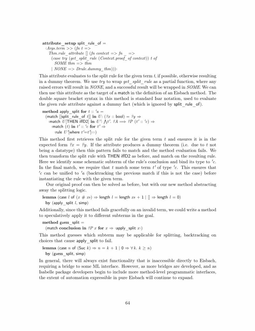
attribute_setup split_rule_of =〈Args.term >> (fn t =>Thm.rule_attribute [] (fn context => fn _ =>(case try (get_split_rule (Context .proof_of context)) t ofSOME thm => thm| NONE => Drule.dummy_thm)))〉

This attribute evaluates to the split rule for the given term t, if possible, otherwise resultingin a dummy theorem. We use try to wrap get_split_rule as a partial function, where anyraised errors will result in NONE, and a successful result will be wrapped in SOME. We canthen use this attribute as the target of a match in the definition of an Eisbach method. Thedouble square bracket syntax in this method is standard Isar notation, used to evaluatethe given rule attribute against a dummy fact (which is ignored by split_rule_of).

method apply_split for t :: ′a =(match [[split_rule_of t ]] in U : (?x :: bool) = ?y ⇒

〈match U [THEN iffD2] in U ′:∧t ′. ?A =⇒ ?P (t ′ :: ′c) ⇒

〈match (t) in t ′ :: ′c for t ′⇒〈rule U ′[where t ′=t ′]〉〉〉)

This method first retrieves the split rule for the given term t and ensures it is in theexpected form ?x = ?y . If the attribute produces a dummy theorem (i.e. due to t notbeing a datatype) then this pattern fails to match and the method evaluation fails. Wethen transform the split rule with THEN iffD2 as before, and match on the resulting rule.Here we identify some schematic subterm of the rule’s conclusion and bind its type to ′c.In the final match, we require that t match some term t ′ of type ′c. This ensures that′c can be unified to ′a (backtracking the previous match if this is not the case) beforeinstantiating the rule with the given term.

Our original proof can then be solved as before, but with our new method abstractingaway the splitting logic.lemma (case l of (x # xs) ⇒ length l = length xs + 1 | [] ⇒ length l = 0)by (apply_split l , simp)

Additionally, since this method fails gracefully on an invalid term, we could write a methodto speculatively apply it to different subterms in the goal.method guess_split =(match conclusion in ?P x for x ⇒ 〈apply_split x 〉)

This method guesses which subterm may be applicable for splitting, backtracking onchoices that cause apply_split to fail.lemma (case n of (Suc k) ⇒ n = k + 1 | 0 ⇒ ∀ k . k ≥ n)by (guess_split, simp)

In general, there will always exist functionality that is inaccessible directly to Eisbach,requiring a bridge to some ML interface. However, as more bridges are developed, and asIsabelle package developers begin to include more method-level programmatic interfaces,the extent of automation expressible in pure Eisbach will continue to expand.

64

5.3 Design and Implementation

A core design goal of Eisbach is a seamless integration with other Isabelle languages,notably Isar, ML, and object-logics. The primary motivation clearly being to make itaccessible to existing Isabelle/Isar users, with a secondary objective of both forward andbackward compatibility.

5.3.1 Readable Proof Methods

In Isar there is a clear distinction between a structured and an unstructured proof. Theformer makes use of the rich reasoning framework provided by Isar, while the latter reliesmore heavily on the implicit behaviour of proof methods. An unstructured proof cannotbe understood without checking the proof in Isabelle and inspecting the subgoal stateat each stage of the proof. This can create significant issues during proof maintenancephases, where a proof needs to be updated in response to an update to a specification orto Isabelle itself. The original intention of a proof cannot be easily extracted from theunstructured proof script, and a now-failing proof may require significant time and effortto perform the necessary archaeological exploration of its history to recover some insight.

One of the aims of Eisbach is to address this by providing a means to describe reasoningprocedures. A proof method designed to solve a particular class of problems serves as abetter record of the author’s intent than an ad-hoc series of general tools. Arguably thissimply shifts the problem of proof maintenance to that of proof method maintenance, andindeed this is a well-known concern in Ltac today. This indicates the necessity for writingproof methods that are readable and thus also maintainable.

In Eisbach, match can be considered as a structured language element, and is meant toserve both as implementation and documentation. Many methods shown here could havebeen implemented without using match, but would have been significantly more difficult tounderstand, and may happen to work in unintended cases. In practice, a match patternis a much more explicit description of the expected goal state than, for example, theexpectation that erule successfully finds an appropriate premise for the given rule. Aswith Isar, Eisbach method authors are free to use as much structure as they considernecessary for their specific application.

5.3.2 Design Goals and Comparison to Ltac

Here we explicitly revisit the design goals presented in Section 5.1, discussing each in thecontext of both Eisbach and Ltac.

To be easy to use for beginners and experts. Both Eisbach and Ltac meth-ods/tactics can be constructed from tools that users naturally become familiar with whenwriting proofs, thus providing a low barrier-to-entry. In both languages, matching allowsexperts to explicitly introspect the goal state when writing complex tools.

To expose limited functionality, leaving complex functionality to Isabelle/ML.At its core, Eisbach provides the ability to name a method expression and abstract

65

it over parameters. Many Eisbach methods can then be written by simply combiningIsabelle/Isar’s built-in methods. This is similar to the functionality provided by Ltac,however, as opposed to Ltac’s match keyword, Eisbach’s match method is implemented asa stand-alone tool.

Isar’s integration with ML (see Section 5.2.7) makes this a natural design choice, anddemonstrates how similar language extensions can be written by end-users. In contrast,Coq discourages ad-hoc use of OCaml by requiring separate compilation of custom plug-ins.

To be extensible by end-users. In addition to providing new language features bywriting custom ML methods, Eisbach methods can be made extensible through Isar’snamed theorems (see Section 5.2.1), allowing databases of facts to be managed as contextdata. This can be seen as a generalization of the hint databases used by Coq’s auto tactic.

Seamless integration with other Isabelle languages. By forming static closuresof Isar’s existing method syntax (see Section 5.3.4), Eisbach immediately benefits fromexisting methods and Isabelle languages. This underlying functionality can be used toeasily include method expressions as arguments to both (higher-order) methods and othertools. For example, later in Section 6.2 we use this functionality to implement a pair ofrule attributes for transforming proven facts with method expressions.

Although Coq tools can similarly be implemented to take tactics as arguments, thisfunctionality is more immediately expressive in Isabelle/Isar, as methods can be definedto have arbitrarily complex syntax (e.g. match).

To continue Isar’s principle of readable proofs, creating readable proof proce-dures In an Isar proof, authors are free to choose the extent of structured proof elementsto use. Highly structured proofs are generally more easily understood, at the cost of beingmore verbose. Similarly, Eisbach’s match can be used as documentation for the intent ofa particular method.

5.3.3 Method Correctness and Types

In contrast to Coq’s Mtac (see Section 2.1.5), Eisbach and Ltac are untyped languages. ForEisbach, this was a necessary design choice in order to integrate with Isabelle’s existinguntyped tactics and methods. This may seem ironic, given that both ML and Isabelle’sPure logic are strongly typed. Indeed this discussion dates back to the tactical proofs thatfirst appeared in the original LCF proof assistant (see Section 2.1.3).

It is important to clarify that both Ltac and Eisbach are subject to the correctnessconstraints of their respective proof systems. In the case of Eisbach, each defined methodeventually appeals to the primitive inferences of Isabelle’s Pure logic using the proof kernel(see Section 3.2.3). Eisbach methods, like all Isabelle proof tools, can therefore at mostfail to produce a valid proof, without concerns that programming errors will allow forunsound reasoning.

In tactical proving there is therefore less of an immediate need for the static guaranteesthat would be provided by a type system. Instead, we can focus on providing run-time

66

checks, meaningful error messages and interactive debugging facilities (see Section 6.1). InEisbach, intermediate match clauses could explicitly check that the subgoal state has someexpected form before invoking a tool that makes this assumption implicitly. In general,method semantics can be encoded as run-time pre and postcondition checks. For example,a verification-condition generator (see Section 7.1) might have a precondition check thatthe initial subgoal is an annotated program, and a postcondition check that no producedsubgoals discuss the semantics of the original program.

5.3.4 Static Closure of Concrete Syntax

Isabelle provides a rich selection of powerful proof methods, each with its own concretesyntax, which is implemented by parser combinators in ML. Additionally, Isabelle’s theo-rem attributes, which perform context and fact transformations, have their own parsers.Rather than re-write all tools from the libraries to support Eisbach, we build on existingfeatures of the Isabelle parsing framework whereby tokens have values (types, terms, factsetc.) assigned to them implicitly during parsing.

This syntax/value assignment mechanism was originally introduced to support localeexpressions in the sense of [10]. Thus expressions over facts and attributes became trans-formable by morphisms, to move them from an abstract locale context to a concreteapplication context.3

The same principle of syntax closure and interpretation is now the main workhorseof Eisbach. After some modifications, it works for method expressions as well, includingtheir embedded facts and attribute expressions. For example, the basic method “(simpadd : foo [OF bar ])” is wrapped up as static closure, where the embedded fact expression“foo [OF bar ]” is treated like a pre-evaluated constant.

Eisbach then simply serves as an interpretation environment for the carefully preparedmethod syntax tokens. When a proof method is applied, Eisbach instantiates these to-ken values appropriately (via some morphism), based on the supplied arguments to themethod or results of matching, and then executes the resulting method body. Althoughthis presents some technical challenges and required various modifications of the Isar im-plementation itself, this proves to be a very effective solution to performing this kind oflanguage extension.

As a result of this, the inner methods that appear in Eisbach method definitions mayhave arbitrarily complex internal syntax. For example, Eisbach’s match is implemented asa standard proof method, rather than requiring any special status in the language. Thisopens the door for users to develop their own advanced proof methods to serve as languageextensions for method development in Eisbach.

5.3.5 Subgoal Focusing

In Isabelle/Pure there is a logical distinction between universally quantified parameters(like x in

∧x . P x ) and arbitrary-but-fixed terms (like a in P a). A subgoal in the

former form does not allow the x to be explicitly referenced, because it is hidden within3See also [11] for a recent exposition of the possibilities of locales and locale interpretations via mor-

phisms in Isabelle.

67

a closed formula; for example, my_fact [where y = x ] does not produce a valid theorem.Historically, some special tactics were provided to descend into the sub-goal structureand provide ad-hoc access to its local parameters: these are available in Isar via so-calledimproper methods (like rule_tac).

Likewise, premises within a subgoal are not yet local facts. In a structured Isar proof,assumptions are stated explicitly in the text via assumes or assume and are accessibleto attributes etc. In contrast, the local prefix A =⇒ ◊ of a subgoal is not accessible tostructured reasoning and cannot be provided to standard methods as explicit arguments.

Isabelle/ML provides systematic support for subgoal focusing, and Isar provides accessto it via the subgoal command. Focusing creates a new goal out of a given subgoal, butwith its parameters turned into fixed variables (actual terms), and premises into localassumptions (actual facts). For example:

lemma∧A B C . [[(

∧x . A x =⇒ B); B =⇒ C ; A y ]] =⇒ C

subgoal premises prems for A B C

1 . C

At this point the goal has been focused, where the goal parameters (A, B and C ) areconverted into fixed terms, and the subgoal becomes focused on the conclusion (C ). Thegoal premises have been lifted into proper assumptions, lifting meta-universally quantifiedvariables into schematics, and then stored in the local fact prems.thm prems — A ?x =⇒ B, B =⇒ C, A y

We can then complete this proof by referring to prems directly. As prems contains threeindividual theorems (one for each premise in the original goal), we can refer to each directlywith the standard syntax prems(n) for selecting the nth theorem of prems.

apply (rule prems(2))apply (rule prems(1)[where x = y ])apply (rule prems(3))done

doneHere the first done ends the subgoal focus, having successfully discharged the subgoaland the second done concludes the proof.

For Eisbach, we incorporated this into the language with some concrete syntax, to allowthe user to write methods that can operate within the local subgoal structure as required.This allows for uniform treatment of the goal state when matching and parameter passing.In Eisbach’s match method, focusing is accessed by specifying the keyword conclusion orpremises as the match target (see Section 5.2.4).

5.4 Conclusion

In this chapter we have presented Eisbach, a high-level language for writing proof methodsin Isabelle/Isar. It supports familiar Isar language elements, such as method combinatorsand rule attributes, as well as being compatible with existing Isabelle proof methods.

68

An expressive match method enables the use of higher-order matching against facts andsubgoals to provide control flow.

One of Eisbach’s greatest virtues is that it provides a framework for thinking of proofmethods like programming language elements. This applies to methods written in Eisbach,like solves, but also to those written in Isabelle/ML. A good example of the latter is thematch method which, while its implementation is entirely independent of the methodcommand, became necessary to implement only in the presence of Eisbach. The methodlanguage of Isar was already arbitrarily expressive, as methods define their own syntax.Eisbach now opens up this space allowing users to write methods that serve as elements ofa high-level method programming language, rather than one-off proof tools. Thus methodsthat may have had little use in proof scripts now become useful and, in the case of match,powerful, as elements of Eisbach-defined proof methods.

In the next chapter, we will see how Isar and Eisbach can be extended into a richecosystem for proof method development. Later, in Chapter 7, we show how Eisbach canbe used to implement a set of real-world proof methods in L4.verified, and demonstratetheir impact on existing proofs.

69

Chapter 6

Advanced Eisbach

With Eisbach we can rapidly prototype and develop new proof methods by using Isar’sfamiliar method expressions, use named theorems to manage and implicitly use collectionsof facts as proof context data, and perform matching on proof states to manage the controlflow of methods. Although this is sufficient for many use cases, the core infastructure ofEisbach can be used for many advanced applications that were previously not immediatelypossible in Isar.

In particular, Eisbach provides a facility for forming a static closure from a methodexpression (see Section 5.3.4). From this, methods can be treated as first class languageelements, to be easily provided to existing tools as standalone arguments.

In this chapter, we explore both the consequences of this new ability, and demonstratesome of the advanced capabilities of Eisbach. Implementations of the tools presented hereare available in the L4.verified repository [5].

Chapter Outline

• Method Expression Debugging. In Section 6.1 we present a new Isar command,apply_debug, and specialized proof method, #break, that allow for interactivelystepping through the execution of a method expression.

• Rule Attributes from Methods. In Section 6.2 we present a pair of new ruleattributes that allow proof methods to be used as fact transformers.

• Advanced Methods and Combinators. In Section 6.3 we present a suite ofspecialized methods for performing technical operations in proof methods.

6.1 Method Expression Debugging

Although Isabelle’s proof kernel precludes writing proof methods which produce logicallyunsound results, while under development they will often have unexpected or unintendedbehaviour. When a method loops indefinitely, or fails to make progress on a goal, a proofengineer requires tools to discover the source of the problem.

70

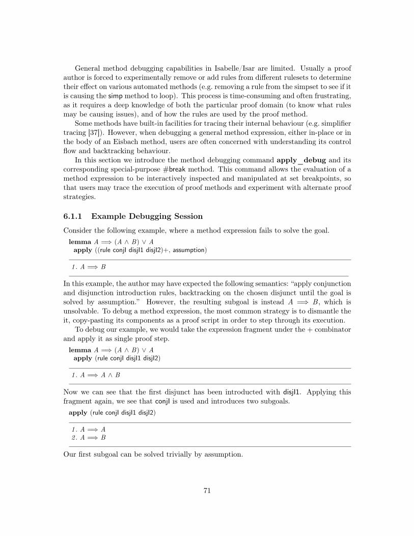
General method debugging capabilities in Isabelle/Isar are limited. Usually a proofauthor is forced to experimentally remove or add rules from different rulesets to determinetheir effect on various automated methods (e.g. removing a rule from the simpset to see if itis causing the simp method to loop). This process is time-consuming and often frustrating,as it requires a deep knowledge of both the particular proof domain (to know what rulesmay be causing issues), and of how the rules are used by the proof method.

Some methods have built-in facilities for tracing their internal behaviour (e.g. simplifiertracing [37]). However, when debugging a general method expression, either in-place or inthe body of an Eisbach method, users are often concerned with understanding its controlflow and backtracking behaviour.

In this section we introduce the method debugging command apply_debug and itscorresponding special-purpose #break method. This command allows the evaluation of amethod expression to be interactively inspected and manipulated at set breakpoints, sothat users may trace the execution of proof methods and experiment with alternate proofstrategies.

6.1.1 Example Debugging Session

Consider the following example, where a method expression fails to solve the goal.lemma A =⇒ (A ∧ B) ∨ Aapply ((rule conjI disjI1 disjI2)+, assumption)

1 . A =⇒ B

In this example, the author may have expected the following semantics: “apply conjunctionand disjunction introduction rules, backtracking on the chosen disjunct until the goal issolved by assumption.” However, the resulting subgoal is instead A =⇒ B , which isunsolvable. To debug a method expression, the most common strategy is to dismantle theit, copy-pasting its components as a proof script in order to step through its execution.

To debug our example, we would take the expression fragment under the + combinatorand apply it as single proof step.lemma A =⇒ (A ∧ B) ∨ Aapply (rule conjI disjI1 disjI2)

1 . A =⇒ A ∧ B

Now we can see that the first disjunct has been introducted with disjI1. Applying thisfragment again, we see that conjI is used and introduces two subgoals.apply (rule conjI disjI1 disjI2)

1 . A =⇒ A2 . A =⇒ B

Our first subgoal can be solved trivially by assumption.

71

apply assumption

1 . A =⇒ B

Now we see the final proof state that was encountered after evaluating the original expres-sion.

The issue in this example is that the first subgoal produced by applying conjI is indeedsolvable by assumption, which terminates the method evaluation and leaves A =⇒ Bto be solved. Since the method has successfully evaluated, no backtracking results areattempted, and the intended strategy of initially applying disjI2 is not explored.

Without additional tool support, debugging Eisbach methods requires a similar strat-egy: copy-pasting sections of method definitions into Isar proofs in order to interactivelytrace their execution.

Consider the following modification of the previous example, where the method expres-sion has been generalized into an Eisbach method. The proof fails as expected, howeverisolating the cause of the error is now much more involved.named_theorems my_solver_rulesmethod my_solver declares my_solver_rules =((rule my_solver_rules)+, assumption)

lemma A =⇒ (A ∧ B) ∨ Aapply (my_solver my_solver_rules: conjI disjI1 disjI2)oops

This attempt fails, as in our initial example. However re-creating the original trace requiresfirst populating the my_solver_rules with Isar’s supply command.lemma A =⇒ (A ∧ B) ∨ Asupply [my_solver_rules] = conjI disjI1 disjI2apply (rule my_solver_rules)apply (rule my_solver_rules)apply assumption

oops

This style of method expression tracing proves to be time-consuming, error-prone, andextremely difficult in non-trivial proofs and method expressions. In larger projects, withmany inter-dependent proof methods, manually constructing a proof trace with this strat-egy becomes nearly impossible.

6.1.2 The apply_debug command

When debugging a proof method we are often faced with two important questions: “Whatis the execution path that lead to the resulting proof state?” and “What alternate strate-gies could be applied in order to make progress?”. Answering the former question allowsus to identify when a method may have made an unexpected or incorrect reasoning step,and the latter gives insight into how a method could be modified in order to resolve theissue.

In this section, we introduce the new Isar command apply_debug. This command

72

takes a method expression and evaluates it against the current proof state, identical tohow the apply command functions. However, it is aware of a special-purpose method#break, which acts as a breakpoint for method evaluation. When a #break is encounteredduring the invocation of apply_debug, the method evaluation halts and the resultingproof state is the intermediate proof state that was seen by the breakpoint. The continuecommand resumes execution, until either the next #break is encountered or the methodexpression terminates.

Returning to our previous example, we can debug our method expression by placing a#break inside the loop.lemma A =⇒ (A ∧ B) ∨ Aapply_debug ((rule conjI disjI1 disjI2, #break)+, assumption)

1 . A =⇒ A ∧ B

Here we see the goal state after apply_debug is not the final state, but rather the goalafter only applying disjI1 (i.e. the method has committed to solving the first disjunct). Ifwe execute continue we can see the result after applying conjI.continue

1 . A =⇒ A2 . A =⇒ B

Finally, if we continue again, method evaluation terminates without encountering anyadditional breakpoints and we are presented with the expected goal.continue

1 . A =⇒ B

Final Result.

The output “Final Result.” indicates that the apply_debug evaluation has finished andit is not possible to continue any more. If the expression is evaluated with apply instead,as part of a proof rather than a debugging session, the #break is ignored and the proofcontinues as usual, resulting in the same final proof state.

The same functionality is available when #break is used in the definition of an Eisbachmethod.method my_solver declares my_solver_rules =((rule my_solver_rules, #break)+, assumption)

lemma A =⇒ (A ∧ B) ∨ Aapply_debug (my_solver my_solver_rules: conjI disjI1 disjI2)continue — 1 . A =⇒ A 2 . A =⇒ Bcontinue — 1 . A =⇒ Boops

In this example, the breakpoint inside of my_solver is hit twice, as in the previous example.In both cases, we were readily able to trace the execution of the expression without needing

73

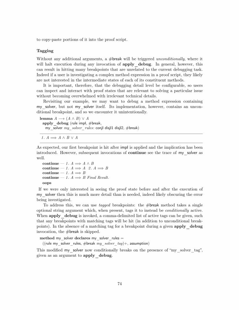
to copy-paste portions of it into the proof script.

Tagging

Without any additional arguments, a #break will be triggered unconditionally, where itwill halt execution during any invocation of apply_debug. In general, however, thiscan result in hitting many breakpoints that are unrelated to the current debugging task.Indeed if a user is investigating a complex method expression in a proof script, they likelyare not interested in the intermediate states of each of its constituent methods.

It is important, therefore, that the debugging detail level be configurable, so userscan inspect and interact with proof states that are relevant to solving a particular issuewithout becoming overwhelmed with irrelevant technical details.

Revisiting our example, we may want to debug a method expression containingmy_solver, but not my_solver itself. Its implementation, however, contains an uncon-ditional breakpoint, and so we encounter it unintentionally.lemma A −→ (A ∧ B) ∨ Aapply_debug (rule impI, #break,my_solver my_solver_rules: conjI disjI1 disjI2, #break)

1 . A =⇒ A ∧ B ∨ A

As expected, our first breakpoint is hit after impI is applied and the implication has beenintroduced. However, subsequent invocations of continue see the trace of my_solver aswell.

continue — 1 . A =⇒ A ∧ Bcontinue — 1 . A =⇒ A 2 . A =⇒ Bcontinue — 1 . A =⇒ Bcontinue — 1 . A =⇒ B Final Result.oops

If we were only interested in seeing the proof state before and after the execution ofmy_solver then this is much more detail than is needed, indeed likely obscuring the errorbeing investigated.

To address this, we can use tagged breakpoints: the #break method takes a singleoptional string argument which, when present, tags it to instead be conditionally active.When apply_debug is invoked, a comma-delimited list of active tags can be given, suchthat any breakpoints with matching tags will be hit (in addition to unconditional break-points). In the absence of a matching tag for a breakpoint during a given apply_debuginvocation, the #break is skipped.method my_solver declares my_solver_rules =((rule my_solver_rules, #break my_solver_tag)+, assumption)

This modified my_solver now conditionally breaks on the presence of “my_solver_tag”,given as an argument to apply_debug.

74

lemma A =⇒ (A ∧ B) ∨ Aapply_debug (tags my_solver_tag)(my_solver my_solver_rules: conjI disjI1 disjI2) — 1 . A =⇒ A ∧ B

continue — 1 . A =⇒ A 2 . A =⇒ Bcontinue — 1 . A =⇒ B Final Result.

We can now debug a method expression that contains my_solver without tracing its exe-cution. By giving no tags to apply_debug, only unconditional breakpoints are encoun-tered.lemma A −→ (A ∧ B) ∨ Aapply_debug (rule impI, #break,my_solver my_solver_rules: conjI disjI1 disjI2,#break) — 1 . A =⇒ A ∧ B ∨ Acontinue — 1 . A =⇒ Bcontinue — 1 . A =⇒ B Final Result.

6.1.3 Proof state interaction

So far we have only used apply_debug to observe the goal state during the execution of amethod expression evaluation. Importantly, however, it also grants the ability to interactdirectly with the run-time proof state: the proof context can be examined with standardIsar diagnostic commands (e.g. thm and term), and the goal state can be modified ad-hocwith proof methods. Each #break provides an opportunity for the user to interact withthe intermediate state in a proof method evaluation as if it were an intermediate state ina proof script.

Returning to our example, we can use thm to examine the contents of thenamed_theorem my_solver_rules during the execution of my_solver.

lemma A =⇒ (A ∧ B) ∨ Aapply_debug (tags my_solver_tag)(my_solver my_solver_rules: conjI disjI1 disjI2)continue

1 . A =⇒ A2 . A =⇒ B

thm my_solver_rules

[[?P ; ?Q ]] =⇒ ?P ∧ ?Q?P =⇒ ?P ∨ ?Q?Q =⇒ ?P ∨ ?Q

Additionally, we may apply methods to modify the run-time state. In this state, for exam-ple, if we manually apply assumption, we can trigger the desired backtracking behaviourfrom the expression.

75

apply assumption

1 . A =⇒ B

Since the first subgoal is now solved, the assumption from the body of my_solver will failon the new head subgoal, causing the method to explore other backtracking branches.continue

1 . A =⇒ A

The method has backtracked and applied disjI2 instead, breaking afterwards. Now if wecontinue, the assumption from my_solver successfully solves the goal and the methodexecution finishes.continue

No subgoals!

Final Result.

Our debugging session has now altered the outcome of the method evaluation, resultingin a successful proof.

With this, we have both identified the source of the error, and a potential solution: byrequiring that all emerging subgoals be solvable by assumption, we force the backtrackingbehaviour of the method to explore all possible combinations of the given rules. This canbe accomplished by replacing sequential composition (,) with structured concatenation (;).Implementing this change in an updated my_solver successfully solves the original goal.method my_solver_fixed declares my_solver_rules =((rule my_solver_rules)+; assumption)

lemma A =⇒ (A ∧ B) ∨ Aapply (my_solver_fixed my_solver_rules: conjI disjI1 disjI2)done

Methods as Breakpoint Filters

In addition to using tagged breakpoints, we can further control the breakpoints that areencountered by providing continue with a method as an optional argument. This methodacts as a filter against the proof state at each breakpoint, and only halts the evaluationof the debugged method expression if the given method successfully applies to the proofstate.

Consider the following example, where structured concatenation has been used to breakon each subgoal produced by intro conjI.

76

lemma A ∧ (∀ x . P x ) ∧ B ∧ Capply_debug (#break, (intro conjI; #break)) — 1 . A ∧ (∀ x . P x ) ∧ B ∧ Ccontinue — 1 . Ccontinue — 1 . Bcontinue — 1 . ∀ x . P xcontinue — 1 . Acontinue — 1 . A 2 . ∀ x . P x 3 . B 4 . C

The second #break is executed on a restricted view of the subgoal multiple times, onceper conjunct. Now, consider the case where we are interested in investigating the proofstate prior to encountering a particular conjunct, e.g. ∀ x . P x . If there are a large numberof subgoals, it is impractical to manually continue over each one. One option to addressthis is to conditionally break by using Eisbach’s match method.lemma A ∧ (∀ x . P x ) ∧ B ∧ Capply_debug (#break,(intro conjI; match conclusion in ∀ x . _ ⇒ 〈#break〉 _ ⇒ 〈−〉))

continue — 1 . ∀ x . P xcontinue — 1 . A 2 . ∀ x . P x 3 . B 4 . C Final Result.

Although this strategy is effective in isolating the desired subgoal, it requires modifyingthe method expression itself to do so. To address this, the continue command caninstead be given a single method as an argument, to be used as filter on the proof statesencountered by each break point. The breakpoint is hit if the evaluation of the givenmethod is successful. If the method fails to apply, the breakpoint is skipped.

In our example, we can provide a match as a filter to continue which succeeds onlywhen the conclusion of the goal is a universal quantifier.lemma A ∧ (∀ x . P x ) ∧ B ∧ Capply_debug (#break, (intro conjI; #break))continue (match conclusion in ∀ x . _ ⇒ 〈−〉)

1 . ∀ x . P x

In this session, the first two encounters of #break are skipped since the match fails, andthe continue halts on the intended subgoal ∀ x . P x . Further uses of continue, however,will hit the remaining breakpoints as expected.

continue — 1 . Acontinue — 1 . A 2 . ∀ x . P x 3 . B 4 . C Final Result.

Rather than using match, we could instead apply a rule that distinguishes the targetbreakpoint. Note, however, that the effect of the given method is preserved in the resultingproof state. In our example, we could use allI ((

∧x . ?P x ) =⇒ ∀ x . ?P x ) to halt on ∀ x .

P x and introduce its variable.lemma A ∧ (∀ x . P x ) ∧ B ∧ Capply_debug (#break, (intro conjI; #break))continue (rule allI) — 1 .

∧x . P x

continue — 1 . Acontinue — 1 . A 2 .

∧x . P x 3 . B 4 . C Final Result.

77

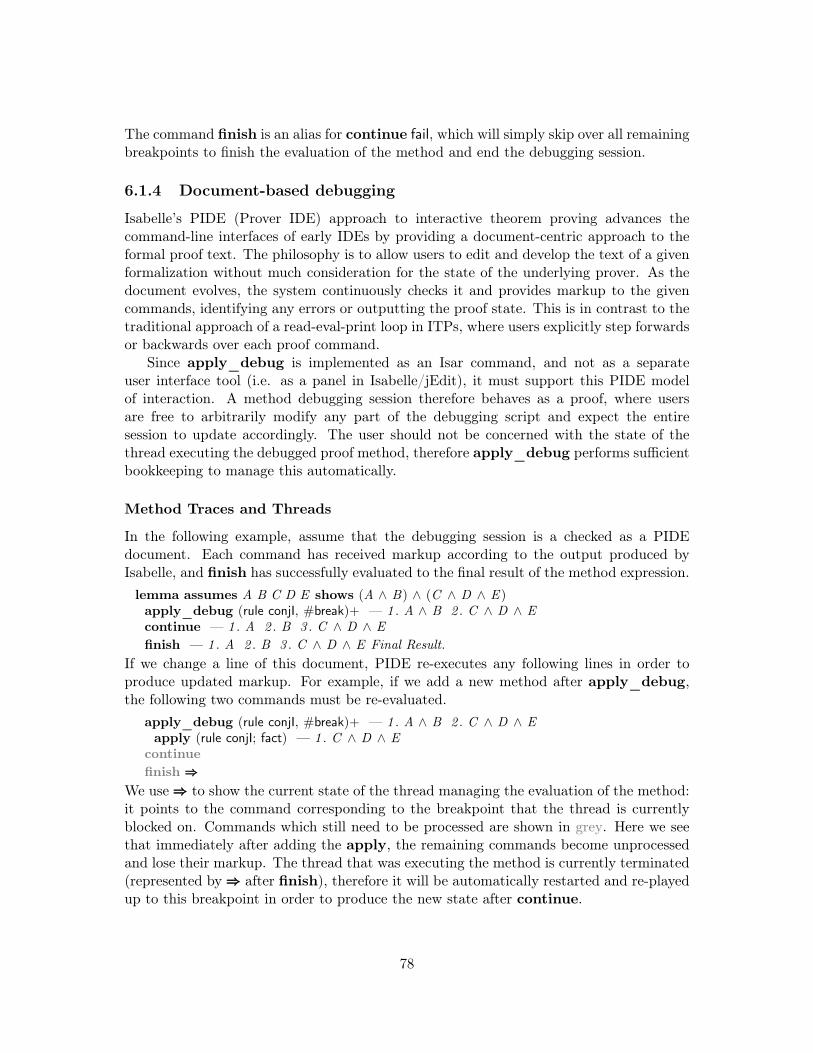
The command finish is an alias for continue fail, which will simply skip over all remainingbreakpoints to finish the evaluation of the method and end the debugging session.

6.1.4 Document-based debugging

Isabelle’s PIDE (Prover IDE) approach to interactive theorem proving advances thecommand-line interfaces of early IDEs by providing a document-centric approach to theformal proof text. The philosophy is to allow users to edit and develop the text of a givenformalization without much consideration for the state of the underlying prover. As thedocument evolves, the system continuously checks it and provides markup to the givencommands, identifying any errors or outputting the proof state. This is in contrast to thetraditional approach of a read-eval-print loop in ITPs, where users explicitly step forwardsor backwards over each proof command.

Since apply_debug is implemented as an Isar command, and not as a separateuser interface tool (i.e. as a panel in Isabelle/jEdit), it must support this PIDE modelof interaction. A method debugging session therefore behaves as a proof, where usersare free to arbitrarily modify any part of the debugging script and expect the entiresession to update accordingly. The user should not be concerned with the state of thethread executing the debugged proof method, therefore apply_debug performs sufficientbookkeeping to manage this automatically.

Method Traces and Threads

In the following example, assume that the debugging session is a checked as a PIDEdocument. Each command has received markup according to the output produced byIsabelle, and finish has successfully evaluated to the final result of the method expression.lemma assumes A B C D E shows (A ∧ B) ∧ (C ∧ D ∧ E )apply_debug (rule conjI, #break)+ — 1 . A ∧ B 2 . C ∧ D ∧ Econtinue — 1 . A 2 . B 3 . C ∧ D ∧ Efinish — 1 . A 2 . B 3 . C ∧ D ∧ E Final Result.

If we change a line of this document, PIDE re-executes any following lines in order toproduce updated markup. For example, if we add a new method after apply_debug,the following two commands must be re-evaluated.

apply_debug (rule conjI, #break)+ — 1 . A ∧ B 2 . C ∧ D ∧ Eapply (rule conjI; fact) — 1 . C ∧ D ∧ E

continuefinish ⇒⇒⇒

We use⇒⇒⇒ to show the current state of the thread managing the evaluation of the method:it points to the command corresponding to the breakpoint that the thread is currentlyblocked on. Commands which still need to be processed are shown in grey. Here we seethat immediately after adding the apply, the remaining commands become unprocessedand lose their markup. The thread that was executing the method is currently terminated(represented by⇒⇒⇒ after finish), therefore it will be automatically restarted and re-playedup to this breakpoint in order to produce the new state after continue.

78

⇒⇒⇒ apply_debug (rule conjI, #break)+ — 1 . A ∧ B 2 . C ∧ D ∧ Eapply (rule conjI; fact) — 1 . C ∧ D ∧ E

continuefinish

When evaluated in the updated document, the continue command detects that the ex-ecuting thread has passed it. This thread is therefore restarted, and the method is re-evaluated, starting with the the initial proof state.

apply_debug (rule conjI, #break)+ — 1 . A ∧ B 2 . C ∧ D ∧ Eapply (rule conjI; fact) — 1 . C ∧ D ∧ E

⇒⇒⇒ continuefinish

Once the first breakpoint is hit, the current proof state (just after having applied (ruleconjI; fact)) is given as its result state. The method execution then continues from thismodified state, and continue evaluates to state of the next breakpoint.

apply_debug (rule conjI, #break)+ — 1 . A ∧ B 2 . C ∧ D ∧ Eapply (rule conjI; fact) — 1 . C ∧ D ∧ E

continue — 1 . C 2 . D ∧ E⇒⇒⇒ finishAt this point the executing thread has caught up to the current document state, so thefinish proceeds as normal: completing the evaluation of the method and terminating thethread.

apply_debug (rule conjI, #break)+ — 1 . A ∧ B 2 . C ∧ D ∧ Eapply (rule conjI; fact) — 1 . C ∧ D ∧ E

continue — 1 . C 2 . D ∧ Efinish ⇒⇒⇒ — 1 . C 2 . D ∧ E Final Result.

In this example, restarting the executing thread was relatively straightforward since wehad only modified the result of the first breakpoint. In general, modifying the documentafter several debugging commands will require skipping over each of their correspondingbreakpoints. Additionally, any ad-hoc changes to the proof state that were made in thedebugging script will need to be preserved.

To accomplish this, each debug command records its initial proof state and the orderthat it appeared during the method’s execution. When the executing thread is restarted,the resulting proof state after each skipped #break is its corresponding previously-storedproof state, preserving the effect of any ad-hoc changes that were made in the document.

For example, if we now add an apply after the continue, the restarted thread needsto recreate the result of (rule conjI; fact) in order to match the document state.

⇒⇒⇒ apply_debug (rule conjI, #break)+ — 1 . A ∧ B 2 . C ∧ D ∧ Eapply (rule conjI; fact) — 1 . C ∧ D ∧ E

continue — 1 . C 2 . D ∧ Eapply fact — 1 . D ∧ E

finishAs before, the executing thread is restarted and the method is evaluated starting withthe initial proof state. When the first breakpoint is encountered, its starting state is 1.A ∧ B 2. C ∧ D ∧ E . The document source that produced the resulting state of this

79

#break, however, has already been processed (i.e. apply (rule conjI; fact)). Rather thanattempting to re-evaluate this Isar source, its resulting state from the previous execution(i.e. 1. C ∧ D ∧ E ) is retrieved from the trace and provided as the result of #break. Themethod evaluation then continues from there.

apply_debug (rule conjI, #break)+ — 1 . A ∧ B 2 . C ∧ D ∧ Eapply (rule conjI; fact) — 1 . C ∧ D ∧ E

⇒⇒⇒ continue — 1 . C 2 . D ∧ Eapply fact — 1 . D ∧ E

finishAfter skipping the first breakpoint, the method evaluation continues until the secondbreakpoint, where the current proof state (after applying fact) is given as its result.

apply_debug (rule conjI, #break)+ — 1 . A ∧ B 2 . C ∧ D ∧ Eapply (rule conjI; fact)— 1 . C ∧ D ∧ E

continue — 1 . C 2 . D ∧ Eapply fact — 1 . D ∧ E

⇒⇒⇒ finishAt this point, the thread has caught up to the document state and finish can be success-fully evaluated by resuming the method evaluation as usual.

apply_debug (rule conjI, #break)+ — 1 . A ∧ B 2 . C ∧ D ∧ Eapply (rule conjI; fact) — 1 . C ∧ D ∧ E

continue — 1 . C 2 . D ∧ Eapply fact — 1 . D ∧ E

finish ⇒⇒⇒ — 1 . D 2 . E

6.2 Rule Attributes from Methods

Isar’s rule attributes (see Section 3.4.5) allow for in-place transformations of facts. Forexample, the built-in attributes where and of are used to instantiate schematic variables ofa fact with given arguments, while OF and THEN compose facts together. These attributesperform precise technical adjustments, in contrast to, for example, the simplified attribute,which rewrites all sub-terms in the fact according to the current simpset (or any providedrules). This enables some automation in fact transformations, but is not sufficient formany applications.

Similar to proof methods, it is often desirable to have domain-specific rule attributes forautomating common rule transformations. However, in comparison to method expressions,Isar’s attribute language is relatively primitive.

For example, an existing lemma may be proven in its uncurried form (i.e. A ∧ B−→ C ) while a further proof may require it to be in its curried form (i.e. A −→ B −→C ). Rather than explicitly stating the curried form and proving it as a consequence ofthe existing lemma, it is more robust and convenient to instead convert a lemma in-placeusing a rule attribute.

Using the built-in THEN attribute and sequential composition of attributes (i.e.[attribute1,attribute2]), we can explicitly apply the curry rule (?P ∧ ?Q −→ ?R =⇒ ?P−→ ?Q −→ ?R) a number of times to curry a given fact.

80

lemma ABCD: ((A ∧ B) ∧ C ) −→ D

thm ABCD[THEN curry] — A ∧ B −→ C −→ D

After applying curry once to ABCD, C is pulled out of the conjunction and into theimplication. Applying curry again yields the desired rule in its fully uncurried form.thm ABCD[THEN curry, THEN curry] — A −→ B −→ C −→ D

In this example, the transformation from the uncurried to curried form of a specific rulewas straightforward. In general, however, these transformations can quickly become non-trivial as lemmas grow larger and more complex. Similar to proof methods, rule attributesare traditionally written in Isabelle/ML, thus presenting a significant barrier-to-entry formany proof authors.

The simplified rule attribute is an existing example of exposing the functionality ofproof methods to rule attributes. Both the attribute and simp method utilize the sameunderlying functionality, however each requires a separate Isabelle/ML implementation,parser and syntax.lemma ABB: A ∧ B ∧ B

thm ABB[simplified] — A ∧ B

lemma A ∧ B ∧ B =⇒ A ∧ B by simp

In this example, both simplified and simp implicitly apply the rule conj_absborb ((?A ∧?A) = ?A).

Generalizing this concept, we present a pair of rule attributes that allow proof methodexpressions to be used for performing rule transformations. This exposes the power ofIsabelle’s built-in proof automation to rule attributes, and effectively allows Eisbach to beused as a rule attribute language, as well as a proof method language.

Using methods to transform facts

We can define a specialized rule attribute @ that takes a single method expression as aparameter and evaluates it against the provided rule. With this we can, for example,replicate the functionality of simplified by instead invoking the simp method.thm ABB[@ 〈simp〉] — A ∧ B

Internally (see Section 6.2) this is accomplished by inserting the given fact as the lonepremise of a dummy proof state. The given method expression then performs forwardreasoning on this proof state, taking the final resulting premise as the produced fact. Thedrule method, which replaces a goal premise by resolving it with the first assumption of agiven fact, is therefore equivalent to the THEN attribute.

In our conjunction currying example we needed to apply the THEN attribute a fixednumber of times in order to convert the lemma into its fully curried form. In contrast, thedrule method can be combined with + to apply the given rule as many times as possible.

81

lemma dummy_conclusionapply (insert ABCD)

1 . (A ∧ B) ∧ C −→ D =⇒ dummy_conclusion

apply (drule curry)+

1 . A −→ B −→ C −→ D =⇒ dummy_conclusion

In this dummy proof, we can see that the given method expression has transformed theinserted fact as desired. However this goal is not solvable, thus this transformation cannotbe exported in a usable form. With the @ attribute we can retain this transformation, sothe resulting fact can be used.thm ABCD[@ 〈(drule curry)+〉] — A −→ B −→ C −→ D

Although already an improvement over manually applying THEN, this simple method ex-pression is not sufficient if we wish to have a general-purpose attribute for rule currying. Ifthe antecedent is not left-associated, or if the implication is partially curried, the resultingrule will not be in the desired form.lemma ABCDEFG : (A ∧ B) ∧ (C ∧ D) −→ E ∧ F−→ G

thm ABCDEFG [@ 〈(drule curry)+〉] — A −→ B −→ C ∧ D −→ E ∧ F −→ G

In this example, the method expression successfully curries the first conjunct, but thenthe evaluation terminates since curry is no longer directly applicable via drule. To addressthis, we can use a combination of the uncurry rule (?P −→ ?Q −→ ?R =⇒ ?P ∧ ?Q −→?R) and imp_conj_assoc to re-associate conjunctions in antecedents.

lemma imp_conj_assoc: P ∧ Q ∧ R −→ S =⇒ ((P ∧ Q) ∧ R) −→ S

To complete our transformation, we want to first fully uncurry the rule so we have a singleimplication. After this, we repeatedly re-associate the antecedent until it exposes a singleconjunct and then pull out this conjunct with curry.thm ABCDEFG [@ 〈((drule uncurry)+)? , (drule imp_conj_assoc curry)+〉]

— A −→ B −→ C −→ D −→ E −→ F −→ GSince this method expression performs a general purpose transformation, we may decideto wrap it up in an Eisbach method for easy re-use.method curry_rule = ((drule uncurry)+)? , (drule imp_conj_assoc curry)+

thm ABCDEFG [@ 〈curry_rule〉] — A −→ B −→ C −→ D −→ E −→ F −→ G

Transforming assumptions in facts

Previously, we have seen the @ attribute used to transform the conclusion of a givenfact, by inserting it as a premise to a dummy goal and performing forward reasoning totransform it. Instead, if we wish to transform a fact assumption, we have to performbackwards reasoning.

82

For example, if we instead wanted to curry the implication in the assumption of a rule,we need reverse our reasoning with the OF attribute.lemma ABCD_E: ((A ∧ B) ∧ C ) −→ D =⇒ E

thm ABCD_E[OF uncurry,OF uncurry] — A −→ B −→ C −→ D =⇒ E

This transformation is not possible with the @ attribute. Instead, the # attribute takesmultiple method expressions and applies them in order to the assumptions of the givenfact. In contrast to the @ attribute, the dummy proof state used by # has the assumptioninserted as the conclusion, and thus can be manipulated through backwards reasoning(e.g. the rule method).

thm ABCD_E[# 〈(rule uncurry)+〉] — A −→ B −→ C −→ D =⇒ E

Similar to the previous example, additional consideration would be required to handlenon-trivial implications. We can simply reverse all of the rules to achieve the same trans-formation for rule assumptions.lemma imp_conj_assoc_rev: ((P ∧ Q) ∧ R) −→ S =⇒ P ∧ Q ∧ R −→ S

method curry_rule_asm = ((rule curry)+)? , (rule imp_conj_assoc_rev uncurry)+

This new method curry_rule_asm can now be used to transform rule. assumptions with#.lemma ABCDEFG_H: (A ∧ B) ∧ (C ∧ D) −→ E ∧ F−→ G =⇒ H

thm ABCDEFG_H[# 〈curry_rule_asm〉]

— A −→ B −→ C −→ D −→ E −→ F −→ G =⇒ HIf a rule contains multiple assumptions, each method given to # is evaluated against eachassumption in the order given.lemma ABC_DD_E: [[A ∧ B ∧ C −→ D ; D ∧ D ]] =⇒ E

thm ABC_DD_E[# 〈curry_rule_asm〉 〈simp〉]

— [[A −→ B −→ C −→ D ; D ]] =⇒ E

Of course it is not always straightforward or even possible to perform a given transforma-tion on both the assumptions and conclusion of a given fact. Specifically, the @ attributemay only weaken its conclusion, while # must strengthen its assumptions.lemma AB_CD : A ∨ B =⇒ C ∧ D

thm AB_CD [# 〈rule disjI1〉, @ 〈drule conjunct1〉] — A =⇒ Cthm AB_CD [# 〈rule disjI2〉, @ 〈drule conjunct2〉] — B =⇒ D

Internal Subgoal Structure

Internally, a rule attribute is already very similar to a proof method: both take a thm(see Section 3.2.3) to another thm and are therefore guaranteed by Isabelle’s proof kernel.Isabelle’s LCF tradition embraces the identification of proofs and fact transformations,

83

where a proof is simply a series of fact transformations, with conventions to maintain itssubgoal structure.

In @ and #, the provided method is evaluated against a specially-constructed inter-nal subgoal, such that the result of the evaluation can be used as a new fact. Usingapply_debug we can inspect this subgoal during the method’s evaluation.

Beginning with a dummy proof state, we can trace the evaluation of curry_rule in @by evaluating it as part of a method expression given to apply_debug.

lemma Truethm ABCD — (A ∧ B) ∧ C −→ Dapply_debug (insert ABCD[@ 〈#break, curry_rule, #break〉])

1 . (A ∧ B) ∧ C −→ D =⇒ thesis

When evaluating insert, apply_debug encounters the #break inside of the method givento @ and halts on its internal goal state. To establish this state, @ first introduces a fixedvariable thesis and creates a trivial thm: thesis =⇒ thesis. Treated as a proof state, thishas a single subgoal thesis and overall conclusion thesis.

In this state, the original fact ABCD is inserted into the head subgoal as a goal premise,resulting in internal state ((A ∧ B) ∧ C −→ D =⇒ thesis) =⇒ (thesis). The given methodis then evaluated on this subgoal, as seen at this breakpoint. We can then continue toevaluate curry_rule.continue

1 . A −→ B −→ C −→ D =⇒ thesis

The internal state is now (A −→ B −→ C −→ D =⇒ thesis) =⇒ (thesis), which @will convert into the resulting fact. After the method is completely evaluated, thesis isgeneralized into a schematic ?thesis and then the first subgoal is solved by assumption,instantiating ?thesis to our desired fact. The resulting thm is then simply A −→ B −→C −→ D .continue

1 . A −→ B −→ C −→ D =⇒ True

Final Result.

The initial insert has inserted the final result from @ into the outer proof state. We cantrace the evaluation of the # attribute similarly.lemma Truethm ABCD_E — (A ∧ B) ∧ C −→ D =⇒ Eapply_debug (insert ABCD_E[# 〈#break, curry_rule_asm, #break〉])

1 . (A ∧ B) ∧ C −→ D

To establish this subgoal state, similar to as in @, a fixed variable thesis is introducedand initialized in the trivial proof state thesis =⇒ thesis. The original fact ABCD is then

84

inserted as a premise to the head subgoal, so the internal state is (((A ∧ B) ∧ C −→D =⇒ E ) =⇒ thesis) =⇒ thesis. This thm is then re-associated to produce the desiredsubgoal structure (A ∧ B) ∧ C −→ D =⇒ ((E =⇒ thesis) =⇒ thesis). The head subgoalcan now be transformed with curry_rule_asm.continue

1 . A −→ B −→ C −→ D

After the method has been evaluated, the internal thm is re-associated to ((A −→ B −→ C−→ D =⇒ E ) =⇒ thesis) =⇒ thesis. The fixed thesis is then generalized to a schematicvariable, and the resulting head subgoal is solved by assumption as before. The resultingunderlying thm is the final fact A −→ B −→ C −→ D =⇒ E .continue

1 . (A −→ B −→ C −→ D =⇒ E ) =⇒ True

Final Result.

Additional Arguments

By default, the schematic variables in the given fact are fixed in the internal goal stateto prevent the given method from performing unintended instantiations. To leave themschematic, and able to be instantiated, the flag (schematic) can be given.

thm conjI — [[?P ; ?Q ]] =⇒ ?P ∧ ?Qthm allI — (

∧x . ?P x ) =⇒ ∀ x . ?P x

thm conjI[# 〈rule allI〉] — Error: Failed to apply method to rule assumption.thm conjI[# (schematic) 〈rule allI〉] — [[

∧x . ?P x ; ?Q ]] =⇒ (∀ x . ?P x ) ∧ ?Q

However care must be taken when using this feature, since many methods will aggressivelyinstantiate schematic variables in order to “solve” the internal subgoal.thm conjI[# (schematic) 〈simp〉] — ?Q =⇒ True ∧ ?Q

Additionally, by default, the internal thesis is an object-level judgement (i.e. bool in HOL)in order to maintain compatibility with most methods and rules. This necessitates anextra step performed by these attributes that was not previously discussed, where the rulemust be converted to an object-level judgement (e.g. ∀ x . P x −→ Q x ) prior to the finalinstantiation of thesis, and then have its meta-connectives restored in the final fact (e.g.∧x . P x =⇒ Q x ).Since converting a given fact into an object logic judgement is not always possible (i.e.

if the rule contains meta-logic judgements), the flag (raw_prop) can be given to insteadhave thesis be of type prop.thm conjunctionD1 — PROP ?A &&& PROP ?B =⇒ PROP ?A

thm conjunctionD1[@ 〈−〉] — Error: Failed to fully atomize result.thm conjunctionD1[@ (raw_prop) 〈−〉] — PROP ?A &&& PROP ?B =⇒ PROP ?A

85

This, however, can cause incompatibilities with existing rules and methods (e.g. elimina-tion rules with erule, where the conclusion is a object logic judgement). In this example,the schematic ?R in allE is a bool, so it cannot be applied when the conclusion of the goalis a prop.thm allE — [[∀ x . ?P x ; ?P ?x =⇒ ?R]] =⇒ ?R

thm allI[@ 〈erule allE〉] — (∧x . ?P x ) =⇒ ?P ?x

thm allI[@ (raw_prop) 〈erule allE〉] — Error: Failed to apply method to rule assumption.

Most often these flags are not necessary, but exist to support specific use cases.In Chapter 7 we show a nontrivial application of these attributes, where a large library

of lemmas, stated in the original refinement calculus of L4.verified [23], can be automati-cally transformed into the calculus of a new proof method.

6.3 Advanced Methods and Combinators

With Eisbach it is straightforward to lift existing tacticals into method combinators, sincemethods can be easily taken as arguments to new (higher-order) methods. For example,the common tactical ALLGOALS can be made available to methods with a few lines ofML. This takes a method and repeatedly evaluates it against the goal, once with eachsubgoal rotated to be the head goal.ML〈fun method_evaluate text ctxt facts =

Method .NO_CONTEXT_TACTIC ctxt(Method .evaluate_runtime text ctxt facts)〉

method_setup all =〈Method .text_closure >> (fn m => fn ctxt => fn facts =>letfun tac i st ′ =Goal .restrict i 1 st ′|> method_evaluate m ctxt facts|> Seq .map (Goal .unrestrict i)

in SIMPLE_METHOD (ALLGOALS tac) facts end)〉

This method takes a method as an argument with the Method.text_closure parser. Thisforms a static closure of the method syntax (see Section 5.3.4) which is then re-evaluatedby Method.evaluate_runtime on each subgoal. These functions were introduced to Isar’sMethod module as of Isabelle-2016 in an effort to standardize this aspect of Eisbach.lemma [[A; B ; C ]] =⇒ A ∧ B ∧ Capply (intro conjI)

1 . [[A; B ; C ]] =⇒ A2 . [[A; B ; C ]] =⇒ B3 . [[A; B ; C ]] =⇒ C

Each of these three subgoals is now solvable by assumption.

86

apply (all 〈assumption〉)

doneSome new methods which have no analogous tactical can be extremely useful for writingmethods in Eisbach. For example, we can define a succeeds method combinator whichleaves the goal unchanged, but fails if the method would not have applied.method_setup succeeds =〈Method .text_closure >> (fn m => fn ctxt => fn facts =>letfun can_tac st =(case SINGLE (method_evaluate m ctxt facts) st of

SOME _ => Seq .single st| NONE => Seq .empty)

in SIMPLE_METHOD can_tac facts end)〉

This allows for writing methods that function as tests, when more complex control flow isrequired.

Many general-purpose combinators can be written without requiring ML. For example,we can write a combinator to hide the conclusion of a subgoal from a given method byusing only Eisbach’s match.lemma A ∧ A =⇒ B ∧ Bapply (only_asm 〈simp〉)

1 . A =⇒ B ∧ B

This new method only_asm (defined below) wraps the subgoal such that simp can onlysee the premise A ∧ A, thus leaving the conclusion untouched.

To implement only_asm, first we establish a new context in order to write privatewrapper definitions and lemmas. This allows us to assume that the method passed toonly_asm will be unable to unfold these definitions, or otherwise inadvertently make useof them, since they will necessarily be out of scope.contextbegin

private definition protect_concl x ≡ ¬ xprivate definition protect_false ≡ False

private lemma protect_start: (protect_concl P =⇒ protect_false) =⇒ Pprivate lemma protect_end: protect_concl P =⇒ P =⇒ protect_false

Here we are simply wrapping negation and False, in order to carefully move the conclusionof a subgoal as a negated premise, as in the rule ccontr ((¬ ?P =⇒ False) =⇒ ?P). Thisallows us to use the subgoal focusing provided by match to hide it.

87

method only_asm methods m =(match premises in H [thin]:_ (multi) ⇒

〈rule protect_start,match premises in H ′[thin]:protect_concl _ ⇒

〈insert H , #break, (m, #break);rule protect_end[OF H ′]〉〉)

endIn this method match is used to control the goal premises that m can see. The bound factH holds the goal’s initial premises (binding to all premises due to the multi flag), whileH’ holds the newly-introduced protect_concl premise after applying protect_start. Byremoving protect_concl from the subgoal state with thin (see Section 5.2.5) and bindingit to H’, we ensure that m cannot inadvertently remove or manipulate it, and that theoriginal goal can therefore be restored with protect_end. Additionally, since we are in alocal context, our private lemmas and definitions are inaccessible after the end.

With apply_debug, we can inspect the goal state just before the given method isevaluated.lemma A ∧ A =⇒ B ∧ Bapply_debug (only_asm 〈simp〉)

1 . A ∧ A =⇒ protect_false

Here we can see that B ∧ B has been replaced with protect_false, and that H’ containsthe wrapped conclusion.thm H ′ — protect_concl (B ∧ B)

continue

1 . A =⇒ protect_false

After simp is evaluated, the resulting state has is premise simplified but leaves protect_falseuntouched.continue

1 . A =⇒ B ∧ B

Final Result.

Finally, protect_false has been replaced with B ∧ B , the original conclusion.This pattern of window reasoning turns out to be extremely powerful when combined

with Eisbach, where a combinator focuses the effect of a given method on a sub-componentof the subgoal. In the next section, we’ll see how this can be generalized to write windowreasoning combinators for different proof calculi.

6.3.1 A Hoare Logic Combinator

We have seen how Eisbach can be used to write a general-purpose method combinatoronly_asm that controls the perspective the provided method has on the goal state. This

88

suggests a general strategy for extending this technique to other domains: wrap a subgoalto focus on a particular sub-component, execute the provided method, then unwrap torecover the original structure.

As an example, we can consider the monadic Hoare logic framework used inL4.verified [23]. In this framework, a Hoare triple {|P |} f {|Q |} states that given theprecondition P, the postcondition Q will hold after executing f.{|P |} f {|Q |} ≡ ∀ s. P s −→ (∀ (r , s ′)∈fst (f s). Q r s ′)

A Hoare triple is usually encountered as the conclusion to a subgoal, where the precon-dition is a schematic variable, and the postcondition is a (potentially large) conjunctionresulting from using a verification condition generator. These conjuncts need to be prop-agated into the precondition by applying appropriate rules from the calculus.

Often it is the case that a given Hoare triple requires a very specific or technicaladjustment in order for a proof to proceed. If this cannot be accomplished with existingcalculus rules, the user must resort to manually specifying the desired postcondition, thenprove that it implies the target one. In large proofs, with dozens of individual conjunctsin a postcondition, this can result in excessively verbose and brittle proof scripts.

For example, consider the following scenario:lemma assumes AA ′:

∧r s. A r s =⇒ A ′ r s

shows {|P |} f {|λr s. A r s −→ B r s|}apply (rule hoare_strengthen_post[where Q=λr s. A ′ r s −→ B r s])

1 . {|P |} f {|λr s. A ′ r s −→ B r s|}2 .

∧r s. A ′ r s −→ B r s =⇒ A r s −→ B r s

By manually applying hoare_strengthen_post ([[{|?P |} ?a {|?Q |};∧r s. ?Q r s =⇒ ?R

r s]] =⇒ {|?P |} ?a {|?R|}) and instantiating ?Q to our desired postcondition, we haveintroduced two new subgoals: we now must show that we can establish A ′ r s −→ B r sas the postcondition for f, and that it implies the original condition. The second goal is atrivial consequence of the assumption.

deferapply (simp add : AA ′)

1 . {|P |} f {|λr s. A ′ r s −→ B r s|}

The problem, as stated earlier, is that quoting the postcondition in the proof script isoften impractical. Instead, we would like to be able to use the assumption AA ′ directly tostrengthen the subgoal. To accomplish this, we can write a specialized method combinatorthat allows us to treat the postcondition as if it were the conclusion of a subgoal.

Similar to as we did with the only_asm method, we start by opening a new context tocreate private definitions specific to our method implementation.

89

context begin

private definition packed_triple P f r s ≡ ∃ si . P si ∧ (r , s) ∈ fst (f si)

private lemma packed_triple_start:(∧r s. packed_triple P f r s =⇒ Q r s) =⇒ {|P |} f {|λr s. Q r s|}

private lemma packed_tripleE:packed_triple P f r s =⇒ {|P |} f {|λr s. Q r s|} =⇒ Q r s

Here the new constant packed_triple wraps the first half of a Hoare triple, assuming theexistence of an initial state si that satisfies the precondition P and f gives the returnvalue/result state r and s after si. This allows a Hoare triple to be packed by applyingpacked_triple_start, leaving the postcondition as the conclusion. After the goal has beenmodified, it can be unpacked back into a Hoare triple with packed_tripleE. With Eisbach,this is a simple method to define.method post_simple methods m =(rule packed_triple_start,match premises in H [thin]: packed_triple _ _ _ _ ⇒〈#break, m, #break, (atomize (full))? , rule packed_tripleE[OF H ]〉)

Note the use of atomize after m is invoked. This is a built-in method that rewrites thesubgoal into the current object logic (HOL in this case). Any assumptions are turned intoHOL implications, and goal parameters are turned into universally quantified variables.Here this is necessary to ensure that the goal has been completely collapsed into a singleterm that can be packed with packed_tripleE.

With this method, we can easily modify the postcondition of our subgoal in-place.lemma assumes AA ′:

∧r s. A r s =⇒ A ′ r s

shows {|P |} f {|λr s. A r s −→ B r s|}apply_debug (post_simple 〈rule impI, drule AA ′〉)

1 . A r s −→ B r s

The first breakpoint from post_simple shows the goal just before the method is invoked.We can see that the postcondition has indeed been lifted to the conclusion of the headsubgoal. The local fact H contains the introduced packed_triple assumption.thm H — packed_triple P f r s

Our second breakpoint, hit after the method has executed, shows the resulting goal justbefore it is atomized and packed.continue

1 . A ′ r s =⇒ B r s

The resulting Hoare triple is now in the expected form.

90

continue

1 .∧r s. {|P |} f {|λr s. A ′ r s −→ B r s|}

Final Result.

Note that the introduced goal parameters r and s are not present in the subgoal itself,and will be ignored (or removed) by most methods.

A key issue with this implementation is the implicit assumption that the given methodwill produce a single subgoal. Indeed if multiple goals are produced, then our combinatorwill not behave as expected.lemma assumes DA:

∧r s. D r s =⇒ A r s

shows {|P |} f {|λr s. C −→ A r s ∧ B r s|}apply_debug (post_simple 〈rule impI, rule conjI, rule DA〉)continue

1 . C =⇒ D r s2 . C =⇒ B r s

After introducing the conjunct in the postcondition with conjI, the resulting proof statehas one subgoal per conjunct. This additional subgoal causes the method to behaveunexpectedly, since atomize and rule only affect the head subgoal.continue

1 .∧r s. {|P |} f {|λr s. C −→ D r s|}

2 .∧r s. C =⇒ B r s

Final Result.

Although the first subgoal has been correctly packed into the postcondition, the secondhas resulted an unsolvable subgoal.

Addressing this issue turns out to be non-trivial, and a common issue with methoddevelopment in Eisbach, since there are no built-in methods that allow direct control overthe subgoal structure. The solution is a new fold_subgoals method that will wrap allcurrent subgoals into a single meta-conjunction (&&&).

6.3.2 Subgoal Folding

With a few exceptions, the majority of proof methods operate solely on the first (head)subgoal, where the only possible global effects are the instantiation of schematic variables.We can use method combinators, such as structured concatenation (;) or the custom allcombinator, to lift the effect of a given method to multiple subgoals. However, precisecontrol over the subgoal structure is still not immediately accessible.

When using Isabelle’s built-in methods, subgoals are either introduced by applyinga rule with multiple assumptions or discharged by applying a rule with no assumptions.Introducing a new subgoal is therefore a non-reversible effect.

91

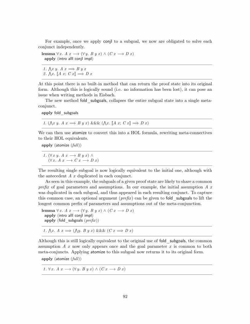
For example, once we apply conjI to a subgoal, we now are obligated to solve eachconjunct independently.lemma ∀ x . A x −→ (∀ y . B y x ) ∧ (C x −→ D x )apply (intro allI conjI impI)

1 .∧x y . A x =⇒ B y x

2 .∧x . [[A x ; C x ]] =⇒ D x

At this point there is no built-in method that can return the proof state into its originalform. Although this is logically sound (i.e. no information has been lost), it can pose anissue when writing methods in Eisbach.

The new method fold_subgoals, collapses the entire subgoal state into a single meta-conjunct.apply fold_subgoals

1. (∧x y . A x =⇒ B y x ) &&& (

∧x . [[A x ; C x ]] =⇒ D x )

We can then use atomize to convert this into a HOL formula, rewriting meta-connectivesto their HOL equivalents.apply (atomize (full))

1 . (∀ x y . A x −→ B y x ) ∧(∀ x . A x −→ C x −→ D x )

The resulting single subgoal is now logically equivalent to the initial one, although withthe antecedent A x duplicated in each conjunct.

As seen in this example, the subgoals of a given proof state are likely to share a commonprefix of goal parameters and assumptions. In our example, the initial assumption A xwas duplicated in each subgoal, and thus appeared in each resulting conjunct. To capturethis common case, an optional argument (prefix ) can be given to fold_subgoals to lift thelongest common prefix of parameters and assumptions out of the meta-conjunction.lemma ∀ x . A x −→ (∀ y . B y x ) ∧ (C x −→ D x )apply (intro allI conjI impI)apply (fold_subgoals (prefix ))

1 .∧x . A x =⇒ (

∧y . B y x ) &&& (C x =⇒ D x )

Although this is still logically equivalent to the original use of fold_subgoals, the commonassumption A x now only appears once and the goal parameter x is common to bothmeta-conjuncts. Applying atomize to this subgoal now returns it to its original form.apply (atomize (full))

1 . ∀ x . A x −→ (∀ y . B y x ) ∧ (C x −→ D x )

92

Focusing while Folding

The effect of fold_subgoals is global to the proof state: all currently visible subgoals arefolded into the resulting meta-conjunct. When performing a subgoal focus (as in a match),only the focused subgoal is visible to the inner method. Applying fold_subgoals in a matchwill therefore only fold subgoals visible in the current focus.lemma assumes DA: D =⇒ Ashows (A ∧ B) ∧ Capply (rule conjI)

1 . A ∧ B2 . C

In a proof state with multiple subgoals, match conclusion will focus on the first one asthe match target. The inner method therefore can only see this goal.

apply_debug(match conclusion in _ ∧ _ ⇒

〈rule conjI, rule DA, #break, fold_subgoals, atomize (full), #break〉)

1 . D2 . B

After applying conjI and DA, in the focused goal, we can fold and atomize to recover asingle subgoal. Note that the third subgoal C from the outer proof state is not visible.continue

1 . D ∧ B

continue

1 . D ∧ B2 . C

Final Result.

After the match been evaluated, the focus ends and we see that the effect of fold_subgoalswas restricted to the head goal, leaving the second subgoal untouched.

Hoare Logic Combinator Revisited

Returning to the Hoare logic example from the previous section, armed with fold_subgoals,it is straightforward to modify our method to simply fold all the resulting subgoals afterapplying m before atomizing.

93

method post methods m =(rule packed_triple_start,match premises in H [thin]: packed_triple _ _ _ _ ⇒〈#break, m, #break,

fold_subgoals (prefix ),(atomize (full))? , #break,rule packed_tripleE[OF H ]〉)

This will now have the intended effect when m produces multiple subgoals.lemma assumes DA:

∧r s. D r s =⇒ A r s

shows {|P |} f {|λr s. C −→ A r s ∧ B r s|}apply_debug (post 〈rule impI, rule conjI, rule DA〉)continue

1 . C =⇒ D r s2 . C =⇒ B r s

After the given method is applied, there are multiple remaining open subgoals. They arethen folded by fold_subgoals into a single goal and atomized.continue

1 . C −→ D r s ∧ B r s

This can now be packed into a single postcondition with packed_tripleE.continue

1 .∧r s. {|P |} f {|λr s. C −→ D r s ∧ B r s|}

Final Result.

Finally, the resulting state is as expected, where the assumption DA has been used totransform one conjunct of the consequent in the postcondition.

6.4 Conclusion

In this chapter we have seen a variety of tools implemented directly in Eisbach (only_asmand post methods), implemented using Eisbach’s method evaluation framework (@ and# attributes), and designed to support proof method development in Eisbach (ap-ply_debug and the fold_subgoals method). These tools both demonstrate the capa-bilities of Eisbach and expand the scope of what is possible with it. In the next chapter,we evaluate this infrastructure in the context of large scale proof engineering by developinga collection of proof methods for real-world use in L4.verified.

94

Chapter 7

Case Study: L4.verified

In the previous chapters we have seen the features provided by the basic Eisbach frame-work and shown how it can be easily extended into a rich ecosystem for developing proofautomation. In this chapter we outline the development of a non-trivial proof methodusing Eisbach. This proof method, corres, is actively being used in the L4.verified projectto aid in its refinement proofs. We show how Eisbach simplifies much of the standardboilerplate for developing proof methods, and how it facilitates rapid prototyping. Weapply the corres method to refactor several existing proofs from L4.verified, resulting insmaller, simpler and more maintainable proofs.

This chapter contains a large amount of technical detail that is not crucial to under-standing the main result, but nonetheless is included for completeness and reproducibility.It assumes a greater degree of familiarity with Isabelle than previous chapters and con-tains many examples with non-trivial proof states. The casual reader can safely read thebeginning of Section 7.1, followed by Section 7.4 and after.

Chapter Outline

• L4.verified, VCGs, and Refinement. Section 7.1 motivates the need for a newproof method in L4.verified for refinement proofs.

• Corres. Section 7.2 introduces the corres refinement calculus from L4.verified.

• The Corres Proof Method. Section 7.3 follows the process of incrementally build-ing a proof method for automating corres proofs

• Application to L4.verified. Section 7.4 presents the results of applying this newmethod to L4.verified.

• Conclusion. Section 7.5 summarizes and puts this case study in the context of thisthesis.

95

7.1 L4.verified, VCGs, and Refinement

The Hoare logic and refinement calculus used in L4.verified [23] were instrumental to itssuccess. Importantly, the VCG (verification-condition generator) for solving Hoare triplesis extensively used in the L4.verified proofs. This VCG, implemented in Isabelle/ML asthe wp method, performs weakest-precondition1 style reasoning [26] to prove invariantproperties about the seL4 microkernel. These invariants are then used as a stepping stonefor the major verification result: proving refinement between seL4’s abstract functionalspecification and its C implementation. This proof provides guarantees about the imple-mentation, such as the absence of invalid memory accesses, but also allows for additionalproperties to be proven against the abstract specification (such as integrity [61] and con-fidentiality [53]) and have them carried down to the implementation without significantadditional effort.

The refinement calculus used in L4.verified is substantially more complicated than theHoare logic. It is contextual refinement under preconditions, and therefore incorporatesHoare logic in order to solve and propagate additional refinement conditions. Ratherthan pay the initial cost of developing a VCG for refinement proofs, however, the originalL4.verified authors instead chose to perform these proofs manually. This decision wasmade for a number of reasons:

• There was no previous work (in contrast to Hoare logic) in developing refinementVCGs.

• Early attempts at developing a refinement VCG were unsuccessful due to frequentchanges to the refinement calculus.

• It was not clear that the initial effort to build a and maintain proof method inIsabelle/ML could be justified given the project’s time-frame.

In the years since the completion of the original proof, these refinement proofs have un-dergone numerous maintenance iterations, and have grown in complexity as seL4 evolved.These highly manual proofs have proven to be among the most brittle in the L4.verifiedproject, as even minor changes to specifications or lemma statements would then requiremanual intervention by a proof engineer.

We therefore decided to develop a new VCG for automating refinement proofs inL4.verified. The goal was to design a VCG that could accelerate the tediously manualprocess of locating and applying rules from the refinement calculus, while also automati-cally attempting some of the advanced proof techniques that had emerged over time. ThisVCG would need to be applicable for refactoring existing refinement proofs to make themmore robust, lowering the cost of proof maintenance, and for accelerating the developmentof new refinement proofs.

The result was the corres proof method, which borrows heavily from weakest-precondition style reasoning for Hoare logic. This method is not necessarily specific to theL4.verified refinement proofs, and indeed is applicable in any refinement proof formalised in

1The preconditions calculated by wp are not necessarily the weakest possible. Occasionally these arereferred to as the weakest reasonable preconditions.

96

the monadic refinement calculus from Cock, et al. [23] (e.g. an abstract specification builton the output of AutoCorres [33]). However, the L4.verified proofs remain the canonicalapplication of this calculus to date.

7.1.1 Refinement

Here we present refinement as defined by Cock et al. in their previous work [23] on for-malizing the Hoare logic and refinement calculus used in L4.verified. Refinement is arelationship between two processes: an abstract (A) and a concrete (C ). We say that Ais refined by C if all possible observable behaviours of C are subsumed by the possiblebehaviours of A, given the same set of inputs. Formally, we can define a process as havingthree functions: an initialization function (Init) which takes an external state into a setof internal states, a step function (Step) which takes an external event and gives a set ofinternal state transitions, and a finalize function (Fin), which takes an internal state andgives a corresponding external state.record process =

Init :: ′external ⇒ ′state setStep :: ′event ⇒ ( ′state × ′state) setFin :: ′state ⇒ ′external

From this we can define an execution function, which evaluates a given process A on somelist of events.steps δ s events ≡ foldl (λstates event . (δ event) ‘‘ states) s eventsexecution A s events ≡ (Fin A) ‘ (steps (Step A) (Init A s) events)

We can then say that A is refined by C if the execution result of C for some given list ofthe events is a subset of the execution of A.A v C ≡ ∀ s events. execution C s events ⊆ execution A s events

Importantly, refinement is transitive, which allows for multiple formal specifications atdifferent levels of abstraction.∀A B C . A v B −→ B v C −→ A v C

To prove refinement, it is often more convenient to instead show the equivalent property offorward simulation. To prove forward simulation between two processes, we first establishan explicit state relation (S ) between the internal states of each one. We then show thateach of the functions that the process comprises establish and maintain this relation.A vS C ≡(∀ s. Init C s ⊆ S ‘‘ Init A s) ∧(∀ event . (S ;; Step C event) ⊆ (Step A event ;; S )) ∧(∀ s s ′. (s, s ′) ∈ S −→ Fin C s ′ = Fin A s)

Roughly, the definition of A vS C says: given a state relation S, a concrete process Cand an abstract process A, A is a forward simulation of C given the following conditions:

• For any external state, the set of initial states for C is a subset of those for A,modulo the state relation S.

• For any single event, the result of stepping C is a subset of stepping A, modulo thestate relation S.

97

• For any two internal states satisfying S, their external final states are equivalent forboth C and A.

It is straightforward to prove that forward simulation implies refinement.∀A C . ∃S . A vS C −→ A v C

Recall from Section 3.5 that L4.verified is divided into two separate refinement proofs,linked by transitivity: C-to-executable (CRefine) and executable-to-abstract (Refine). Thefocus of our case study is the latter proof, which comprises over 80,000 lines of Isabelle/Isarsource to date. Our aim is to increase level of proof automation in the existing executable-to-abstract refinement proof, and to expedite similar proofs in the future.

7.1.2 The State Monad

Both the abstract and executable specifications of L4.verified are formalized as a non-deterministic state monad [23]. The monad state models the entire state of the hardware,including physical memory and machine registers, as well as abstract data structures suchas the kernel heap or capability derivation tree [41]. Each function returns a set of resultstates (and return values), where multiple results represent non-deterministic choice (toabstract away implementation details). To indicate catastropic failure of a function (e.g.invalid memory access), a flag is added to the state which is tripped if any possiblecomputation branch would fail.

( ′s, ′a) nondet_monad = ′s ⇒ ( ′a × ′s) set × bool

The basic monad constructors are return and bind (>>=)). The return constructor takesa single argument and immediately returns it, leaving the state unmodified and alwayssucceeding (leaving the failure flag False).

return :: ′a ⇒ ′s ⇒ ′a × ′s set × boolreturn a ≡ λs. ({(a, s)}, False)

Monadic bind takes two functions, f and g, and composes them in sequence. The inputstate s is evaluated on f, and the set of resulting state-return value pairs (s’ and r) aregiven to g. The final result is the union of all the possible results of g.>>= :: ( ′s, ′a) nondet_monad ⇒ ( ′a ⇒ ( ′s, ′b) nondet_monad)

⇒ ( ′s, ′b) nondet_monad

f >>= g ≡ λs. (⋃(fst ‘ (λ(s ′,r). g s ′ r) ‘ fst (f s)),

True ∈ snd ‘ (λ(s ′,r). g s r) ‘ fst (f s) ∨ snd (f s))

The failure flag is set to True if any branch of g or f failed. Failure is therefore prolific,and a non-failure result of some function guarantees that none of its non-deterministicbranches will result in failure. The do syntax from Haskell is supported, to make longerchains of computations more concise and readable:do x ← f ; g x od ≡ f >>= g

98

The three canonical monadic laws for return are as follows:

return x >>= f = f xm >>= return = m

(m >>= f ) >>= g = m >>= (λx . f x >>= g)

To interact with the state we require two primitives: gets and modify, which allow forretrieving and modifying respectively.gets :: ( ′s ⇒ ′a) ⇒ ( ′s, ′a) nondet_monadgets f = (λs. ({(f s, s)}, False))

modify :: ( ′s ⇒ ′s) ⇒ ( ′s, unit) nondet_monadmodify f ≡ λs. ({((), f s)}, False)

The monadic laws for gets and modify are similar to those for return.

7.1.3 Monadic Hoare Logic

In L4.verified, Hoare logic is used extensively to prove invariant properties about theabstract and executable specifications. These invariants are necessary conditions for re-finement, and are used to discharge intermediate subgoals arising from the corres calculus(see Section 7.2).

The Hoare triple {|P |} f {|Q |} (briefly introduced previously in Section 6.3.1) statesthat given the precondition P, the postcondition Q will hold after executing f.{|P |} f {|Q |} ≡ ∀ s. P s −→ (∀ (r , s ′)∈fst (f s). Q r s ′)

Note that Q takes two parameters: the return value of f and the resulting state. The rulefor return is straightforward:

return_wp: {|P x |} return x {|P |}

Since return leaves the state unmodified, any predicate P will be preserved by it. Similarrules for gets and modify can be easily proven.

gets_wp: {|λs. P (f s) s|} gets f {|P |}modify_wp: {|λs. P () (f s)|} modify f {|P |}

The rule for bind however is complicated by the need for a fresh predicate.seq: [[

∧x . {|B x |} g x {|C |}; {|A|} f {|B |}]] =⇒ {|A|} f >>= g {|C |}

In seq the intermediate predicate B serves as both the precondition for g and postconditionfor f. Since B does not appear in the conclusion of the goal, we are free to choose anysuitable condition, provided it is sufficient for g to establish C and can be establishedby f. Determining these intermediate conditions (and proving they satisfy the conditionsof seq) is the main challenge in automating Hoare logic proofs. A verification-conditiongenerator takes a Hoare triple and applies seq and similar rules from the Hoare logiccalculus, calculating and connecting the intermediate conditions in order to produce afinal verification condition, whose proof ultimately entails the validity of the Hoare triple.

99

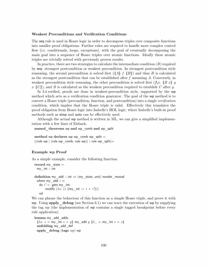
Weakest Preconditions and Verification Conditions

The seq rule is used in Hoare logic in order to decompose triples over composite functionsinto smaller proof obligations. Further rules are required to handle more complex controlflow (i.e. conditionals, loops, exceptions), with the goal of eventually decomposing themain goal into a sequence of Hoare triples over atomic functions. Ideally these atomictriples are trivially solved with previously proven results.

In practice, there are two strategies to calculate the intermediate condition (B) requiredby seq: strongest postcondition or weakest precondition. In strongest postcondition stylereasoning, the second precondition is solved first ({|A|} f {|B |}) and thus B is calculatedas the strongest postcondition that can be established after f assuming A. Conversely, inweakest precondition style reasoning, the other precondition is solved first (

∧x . {|B x |} g

x {|C |}), and B is calculated as the weakest precondition required to establish C after g.In L4.verified, proofs are done in weakest-precondition style, supported by the wp

method which acts as a verification condition generator. The goal of the wp method is toconvert a Hoare triple (precondition, function, and postcondition) into a single verificationcondition, which implies that the Hoare triple is valid. Effectively this translates theproof obligation from Hoare logic into Isabelle’s HOL logic, where Isabelle’s built-in proofmethods such as simp and auto can be effectively used.

Although the actual wp method is written in ML, we can give a simplified implemen-tation with a few lines of Eisbach.named_theorems wp and wp_comb and wp_split

method wp declares wp wp_comb wp_split =((rule wp | (rule wp_comb, rule wp)) | rule wp_split)+

Example wp Proof

As a simple example, consider the following function:record my_state =my_int :: int

definition my_add :: int ⇒ (my_state, unit) nondet_monadwhere my_add i ≡do i ′← gets my_int;

modify (λs. (s (|my_int := i + i ′|)))od

We can phrase the behaviour of this function as a simple Hoare triple, and prove it withwp. Using apply_debug (see Section 6.1) we can trace the execution of wp by supplyingthe tag wp (the implementation of wp contains a single tagged breakpoint before everyrule application).lemma my_add_adds:{|λs. z = my_int s + y |} my_add y {|λ_ s. my_int s = z |}unfolding my_add_defapply_debug (tags wp) wp

100

The first step in a wp proof to apply the following weakening rule hoare_pre.

hoare_pre: [[{|P ′|} f {|Q |};∧s. P s =⇒ P ′ s]] =⇒ {|P |} f {|Q |}

This replaces the concrete precondition in the current subgoal with a schematic one,ultimately to be established as the consequent in the verification condition.

1 . {|?Q |} do i ′← gets my_int;modify (λs. s(|my_int := y + i ′|))

od{|λ_ s. my_int s = z |}

2 .∧s. z = my_int s + y =⇒ ?Q s

Then seq is applied to introduce an intermediate condition and decompose the functionbody into two Hoare triples.continue

1 .∧i ′. {|?B3 i ′|} modify (λs. s(|my_int := y + i ′|)){|λ_ s. my_int s = z |}

2 . {|?Q |} gets my_int {|?B3 |}3 .

∧s. z = my_int s + y =⇒ ?Q s

The first Hoare triple is solved with modify_wp.continue

1 . {|?Q |} gets my_int {|λi ′ s. my_int (s(|my_int := y + i ′|)) = z |}2 .

∧s. z = my_int s + y =⇒ ?Q s

The second is solved by gets_wp.finish

1 .∧s. z = my_int s + y =⇒ my_int (s(|my_int := y + my_int s|)) = z

Final Result.

At this point the method terminates, as the verification condition has been successfullygenerated. This goal is a trivial consequence of Isabelle’s records, and can be solved bysimp.by simp

The wp attribute

The wp declaration attribute (see Section 3.4.4) can be used to manage a database of Hoaretriples, to be automatically applied by the wp method. Each conjunct in a compositepostcondition is matched against this database using Isabelle’s usual rule resolution. Thewp rule set also contains calculational rules for handling control flow, exception handling,

101

etc. For example, if we declare my_add_adds as a wp rule we can then solve Hoare triplescontaining my_add with wp:declare my_add_adds[wp]

lemma{|λs. my_int s = 0|}domy_add 1;my_add 1

od{|λ_ s. my_int s = 2|}by (wp | simp)+

In the ideal case, solving a Hoare triple simply requires a single invocation of wp, followedby a manual proof of the calculated verification condition. If this fails, however, proofauthors must then determine either what rules need to be marked with the wp attributein order for the wp method to succeed, or if manual intervention is required (e.g. a loopinvariant must be explicitly provided).

As more rules are added to this wp database, the wp method becomes capable ofgenerating verification conditions with minimal manual intervention.

7.2 Corres

To prove forward simulation between the abstract and executable specifications ofL4.verified, we need to decompose the problem in to manageable sub-problems. Herewe present the corres calculus used in L4.verified, originally given by Cock et al. [23] andupdated here. This calculus was designed to prove forward simulation for functions definedover a non-deterministic state monad.

Informally, corres_underlying srel nf nf ′ rrel P P ′ a c states: for any two states s ands ′ satisfying the state relation srel, if P s and P ′ s ′ hold, then every result state of c s ′

has a corresponding result state in a s which satisfies srel and the return-value relationrrel. The flags nf and nf ′ control how failure is treated: if nf is True then a s must notfail (assuming P s), and if nf ′ is True then c s ′ must not fail (assuming P ′ s ′).

corres_underlying srel nf nf ′ rrel P P ′ a c ≡∀ (s, s ′)∈srel .

P s ∧ P ′ s ′ −→(nf −→ ¬ snd (a s)) −→(∀ (r ′, t ′)∈fst (c s ′).∃ (r , t)∈fst (a s).

(t , t ′) ∈ srel ∧ rrel r r ′) ∧(nf ′ −→ ¬ snd (c s ′))

The name corres_underlying is historical: originally this framework was only used for theabstract-to-executable refinement proof for L4.verified, so parameters srel, nf and nf ′

were concretely instantiated in the definition of the corres constant. The corres frameworkhas since been abstracted for use in other projects (e.g. Greenaway’s AutoCorres [33]).

102

To avoid rewriting the existing L4.verified proofs, the base constant was renamed to cor-res_underlying and corres was defined as a special case of it.

corres rrel P P ′ a c ≡ corres_underlying state_relation a_nofail c_nofail rrel P P ′ a c

For the sake of brevity, and without loss of generality, in this chapter we will use corres torefer to corres_underlying srel nf nf ′ with some arbitrary-but-fixed instantiation for srel(state_relation), nf (a_nofail) and nf ′ (c_nofail).

Similar to the seq rule for Hoare logic, we can prove a rule that can be used to distributea corres obligation across bind.

corres_split:[[corres R ′ P P ′ a c;∧

rv rv ′. R ′ rv rv ′ =⇒ corres R (S rv) (S ′ rv ′) (b rv) (d rv ′);{|Q |} a {|S |}; {|Q ′|} c {|S ′|}]] =⇒

corres R (P and Q) (P ′ and Q ′) (a >>= (λrv . b rv)) (c >>= (λrv ′. d rv ′))

As in seq, the intermediate predicates S and S ′ serve as both preconditions and post-conditions. They are calculated as the required preconditions in order to establish corresbetween b and d. The two Hoare triples then show that these conditions are establishedby a and c assuming Q and Q ′ respectively. The relation R ′ is required to hold betweenall return values of a and c by assumption A, therefore it can be assumed to hold betweenthe quantified r and r ′ in assumption B.

Similar to the hoare_pre rule in the previous section, the start of a corres proof requiresthat the provided preconditions be replaced with schematic ones. The most straightfor-ward rule simply weakens both preconditions.

corres_guard_imp:[[corres R Q Q ′ a c;

∧s s ′. [[P s; P ′ s ′; (s, s ′) ∈ state_relation]] =⇒ Q s ∧ Q ′ s ′]] =⇒

corres R P P ′ a cFor elementary functions, we can prove general rules which reduce a corres goal to one ormore HOL obligations, which can be solved with standard proof methods.

corres_return: R a b =⇒ corres R > > (return a) (return b)

Where > is the universal predicate (i.e. > ≡ (λs. True)). With this rule we can showcorres between a pair of abstract and concrete return functions if we can prove that thegiven return value relation R is satisfied by the returned values.

Similarly, we can prove corres rules for get and put.corres_gets:(∧s s ′. [[P s; P ′ s ′; (s, s ′) ∈ state_relation]] =⇒ rrel (f s) (f ′ s ′)) =⇒

corres rrel P P ′ (gets f ) (gets f ′)

Since gets leaves the state unmodified the resulting states will always correspond. Theproof obligation is to therefore show that the return relation rrel is satisfied by the givenstate projections f and f ′, assuming the preconditions and state_relation hold.

corres_modify:(∧s s ′. [[P s; P ′ s ′; (s, s ′) ∈ state_relation]] =⇒ (f s, f ′ s ′) ∈ state_relation) =⇒

corres dc P P ′ (modify f ) (modify f ′)

Here we see that two modify functions will correspond if the modified states that are

103

being stored (i.e. f s and f ′ s ′) satisfy the state_relation. The return-value relation is theuniversal relation (dc ≡ λ_ _. True) since put always returns a unit.

To introduce nondeterminism into monadic specifications (as shown later in Sec-tion 7.2.1) we can use the select primitive, which nondeterministically returns a singleelement from a set and leaves the state unmodified.select A ≡ λs. (A × {s}, False)

This can be seen as a generalization of return (i.e. return a = select {a}). The moststraightforward corres rule for select mirrors the definition of corres.

corres_select:(∧s s ′ b. [[P s; P ′ s ′; b ∈ B ]] =⇒ ∃ a∈A. R a b) =⇒

corres R P P ′ (select A) (select B)

This can then be specialized to return.corres_select_return:(∧s s ′. [[P s; P ′ s ′]] =⇒ ∃ a∈A. R a b) =⇒ corres R P P ′ (select A) (return b)

Note that corres_return, corres_select and corres_select_return do not mentionstate_relation as select and return do not read or modify the monadic state.

Using these and similar rules, we can then proceed to prove corres results over inter-mediate functions in monadic specifications, and compose them to prove refinement of thetop-level entry points.

7.2.1 Example

In this section we will develop an abstract and concrete implementation for a toy schedulerand prove corres between them.

Scheduler Specification

First we define the state for each scheduler.record abstract_state =cur_thread :: thread_idthreads :: thread_id set

record concrete_state =cur_thread ′ :: thread_idthreads ′ :: thread_id list

In both states we store the currently running thread, and in the concrete state we maintainan ordered list of runnable threads while the abstract state leaves it as an unordered set.The relationship between these two states is straightforward to define.definition state_relation ≡ {(s,s ′).cur_thread ′ s ′ = cur_thread s ∧set (threads ′ s ′) = threads s}

Where set is the unordered set of elements in a given list, ie:

104

next_thread_abstract ≡do ts ← gets threads;

select tsod

next_thread_concrete ≡do ts ′← gets threads ′;

return (hd ts ′)

od

dequeue_thread_abstract t ≡modify (λs.s(|threads := (threads s) − {t}|))

dequeue_thread_concrete t ′ ≡modify (λs.s(|threads ′ := removeAll t ′ (threads ′ s)|))

set_cur_thread_abstract t ≡modify(λs. (s(|cur_thread := t |)))

set_cur_thread_concrete t ′ ≡modify(λs. (s(|cur_thread ′ := t ′|)))

Figure 7.1: Intermediate functions for scheduler_abstract and scheduler_concrete

set :: ′a list ⇒ ′a setset [] = ∅set (x · l) = {x} ∪ set l

Next we define our abstract and concrete schedulers.definitionschedule_abstract :: (abstract_state, unit) nondet_monadwhere schedule_abstract ≡do t ← next_thread_abstract;

dequeue_thread_abstract t ;set_cur_thread_abstract t

od

definitionschedule_concrete :: (concrete_state, unit) nondet_monadwhere schedule_concrete ≡do t ′← next_thread_concrete;

dequeue_thread_concrete t ′;set_cur_thread_concrete t ′

odEach scheduler selects a new thread according to its scheduling algorithm (next_thread_*),removes it from the set of schedulable threads (dequeue_thread_*), then marks it asthe current thread (set_cur_thread_*). The definitions for these functions are givenin Figure 7.1.

In the concrete scheduler, next_thread_concrete will simply select the first element ofthe list with the partial function hd.hd :: ′a list ⇒ ′ahd (x · xs) = x

For the abstract scheduler, since our thread pool is unordered, our only option is touse non-determinism via the select function when defining next_thread_abstract.

To dequeue the selected thread in dequeue_thread_concrete, we remove it from thelist of schedulable threads with removeAll.

105

removeAll :: ′a ⇒ ′a list ⇒ ′a listremoveAll x [] = []

removeAll x (y · l) = (if x = y then removeAll x l else y · removeAll x l)

Whereas in dequeue_thread_abstract we can use set difference.

op − :: ′a set ⇒ ′a set ⇒ ′a setA − B = {x ∈ A | x /∈ B}

Scheduler Corres Proof

The most interesting functions in this example are the thread selectors(next_thread_abstract and next_thread_concrete). For these functions to corre-spond, we require that at least one thread can be scheduled (otherwise their behavioursdiverge). To ensure this on both sides, it is sufficient to assume that the concrete listof threads is nonempty (i.e. λs ′. threads’ s ′ 6= []) since this will imply that the abstractset of threads is nonempty via the state relation. We know that there is always anondeterministic branch in next_thread_abstract where the selected thread is the sameas next_thread_concrete, so we set our return relation to equivalence.lemma corres_next_thread:corres (λt t ′. t = t ′) > (λs ′. threads ′ s ′ 6= [])

next_thread_abstract next_thread_concreteunfolding next_thread_abstract_def next_thread_concrete_def

After unfolding the definitions of next_thread_abstract and next_thread_concrete we startour proof by replacing the precondition with a schematic.apply (rule corres_guard_imp)

1 . corres (λt t ′. t = t ′) ?Q ?Q ′

(do ts ← gets threads;select ts

od)(do ts ′← gets threads’;

return (hd ts ′)od)

2 .∧s s ′.[[True; threads’ s ′ 6= []; (s, s ′) ∈ state_relation]]=⇒ ?Q s ∧ ?Q ′ s ′

We now have schematic variables for our corres preconditions in the head subgoal, andtwo additional subgoals showing that they are implied by the given preconditions.

106

apply (rule corres_split)

1 . corres ?R ′3 ?P3 ?P ′3 (gets threads) (gets threads’)2 .

∧ts ts ′.?R ′3 ts ts ′ =⇒corres (λt t ′. t = t ′) (?S3 ts)

(?S ′3 ts ′) (select ts) (return (hd ts ′))3 . {|?Q3 |} gets threads {|?S3 |}4 . {|?Q ′3 |} gets threads’ {|?S ′3 |}5 .

∧s s ′.[[True; threads’ s ′ 6= []; (s, s ′) ∈ state_relation]]=⇒ (?P3 and ?Q3 ) s ∧ (?P ′3 and ?Q ′3 ) s ′

After applying the split rule we get one subgoal for each pair of elementary functions.To solve the first goal we specialize corres_gets to have trivial preconditions, and set thereturn relation to state that each set of schedulable threads is equivalent.apply (rule corres_gets[where P=> and P ′=> and rrel=λts ts ′. set ts ′ = ts])

1 .∧s s ′. [[True; True; (s, s ′) ∈ state_relation]] =⇒ set (threads’ s ′) = threads s

A total of 5 subgoals...

This goal is now a trivial consequence of state_relation and can be solved by unfolding itsdefinition.apply (simp add : state_relation_def)

1 .∧ts ts ′.set ts ′ = ts =⇒corres (λt t ′. t = t ′) (?S3 ts)

(?S ′3 ts ′) (select ts) (return (hd ts ′))2 . {|?Q3 |} gets threads {|?S3 |}3 . {|?Q ′3 |} gets threads’ {|?S ′3 |}4 .

∧s s ′.[[True; threads’ s ′ 6= []; (s, s ′) ∈ state_relation]]=⇒ ((λ_. True) and ?Q3 ) s ∧

((λ_. True) and ?Q ′3 ) s ′

The first corres subgoal is now solved and we are left with the second. However ourreturn-value relation is now instantiated concretely in the goal assumptions (i.e. set ts ′ =ts). This goal can be solved with our previously shown corres_select_return rule, wherewe explicitly assume that the fetched thread set (now the ts bound goal parameter) isnonempty.

107

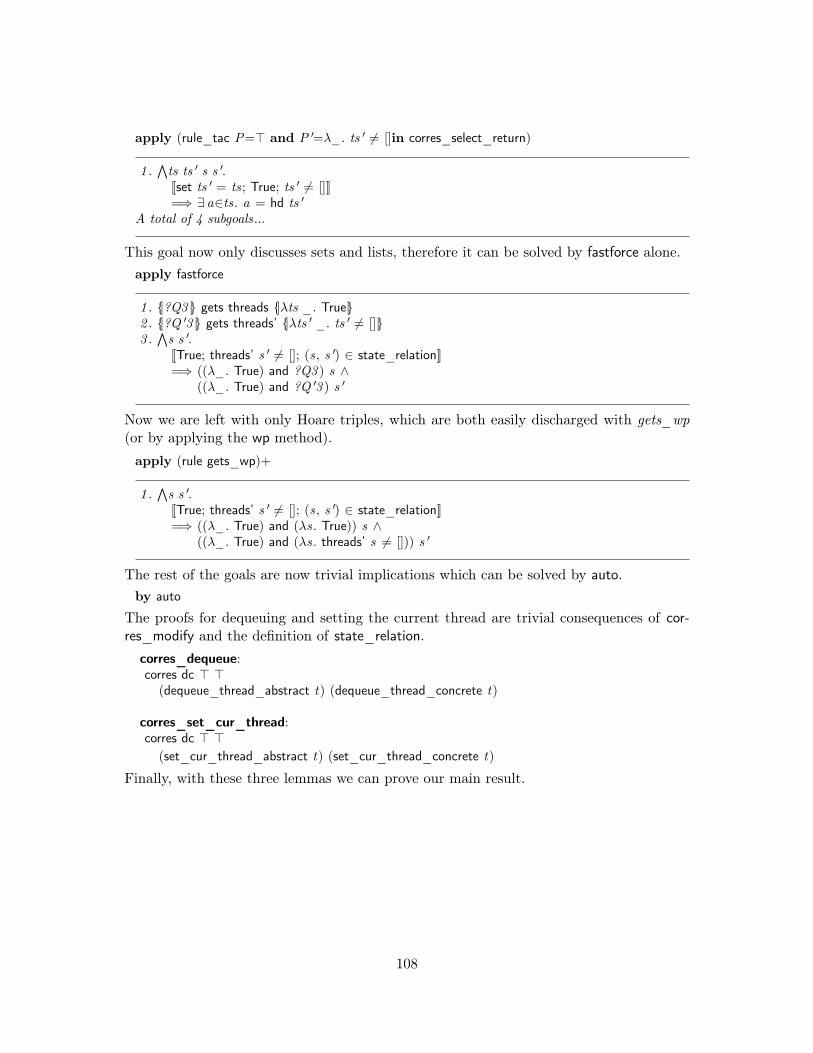
apply (rule_tac P=> and P ′=λ_. ts ′ 6= []in corres_select_return)

1 .∧ts ts ′ s s ′.[[set ts ′ = ts; True; ts ′ 6= []]]=⇒ ∃ a∈ts. a = hd ts ′

A total of 4 subgoals...

This goal now only discusses sets and lists, therefore it can be solved by fastforce alone.apply fastforce

1 . {|?Q3 |} gets threads {|λts _. True|}2 . {|?Q ′3 |} gets threads’ {|λts ′ _. ts ′ 6= []|}3 .

∧s s ′.[[True; threads’ s ′ 6= []; (s, s ′) ∈ state_relation]]=⇒ ((λ_. True) and ?Q3 ) s ∧

((λ_. True) and ?Q ′3 ) s ′

Now we are left with only Hoare triples, which are both easily discharged with gets_wp(or by applying the wp method).

apply (rule gets_wp)+

1 .∧s s ′.[[True; threads’ s ′ 6= []; (s, s ′) ∈ state_relation]]=⇒ ((λ_. True) and (λs. True)) s ∧

((λ_. True) and (λs. threads’ s 6= [])) s ′

The rest of the goals are now trivial implications which can be solved by auto.by auto

The proofs for dequeuing and setting the current thread are trivial consequences of cor-res_modify and the definition of state_relation.

corres_dequeue:corres dc > >

(dequeue_thread_abstract t) (dequeue_thread_concrete t)

corres_set_cur_thread:corres dc > >

(set_cur_thread_abstract t) (set_cur_thread_concrete t)

Finally, with these three lemmas we can prove our main result.

108

lemma corres_schedule:corres dc > (λs ′. threads ′ s ′ 6= [])

(schedule_abstract) (schedule_concrete)unfolding schedule_abstract_def schedule_concrete_defapply (rule corres_guard_imp)apply (rule corres_split)apply (rule corres_next_thread)apply (rule corres_split)

1 .∧t t ′.t = t ′ =⇒corres (?R ′8 t t ′) (?P9 t) (?P ′11 t ′)

(dequeue_thread_abstract t) (dequeue_thread_concrete t ′)A total of 7 subgoals...

Attempting to apply corres_dequeue here directly will fail, since the arguments to eachdequeue function differ (t on the left and t ′ on the right). We first need to simplify thegoal in order to rewrite the conclusion with the assumption (t = t ′) so that our rule will beapplicable (this assumption comes from the return-value relation of corres_next_thread).apply simp

1 .∧t t ′.t = t ′ =⇒corres (?R ′8 t ′ t ′) (?P9 t ′) (?P ′11 t ′)

(dequeue_thread_abstract t ′) (dequeue_thread_concrete t ′)A total of 7 subgoals...

The rest of the proof proceeds as expected, with a similar simplification step requiredfor corres_set_cur_thread.

apply (rule corres_dequeue)apply simpapply (rule corres_set_cur_thread)apply wp+

by auto

7.3 The Corres Proof Method

In this section we will incrementally build a proof method for solving corres proofs us-ing Eisbach. The objective is to demonstrate how a complex method can be iterativelyconstructed using a combination of Eisbach and Isabelle/Isar. To this end, many imple-mentation details have been omitted that appear in the final methods used in L4.verified.The full source of the Eisbach methods, auxiliary Isabelle/ML tools, and proof calculusare available in the L4.verified repository [5].

109

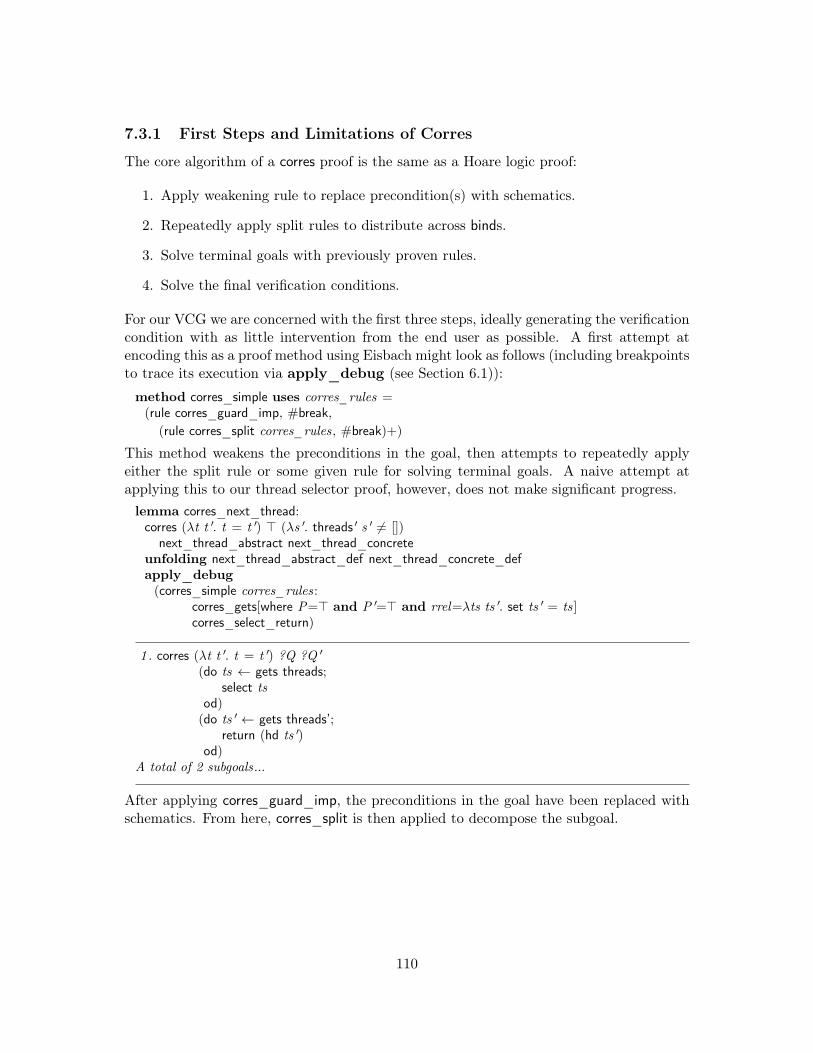
7.3.1 First Steps and Limitations of Corres

The core algorithm of a corres proof is the same as a Hoare logic proof:

1. Apply weakening rule to replace precondition(s) with schematics.

2. Repeatedly apply split rules to distribute across binds.

3. Solve terminal goals with previously proven rules.

4. Solve the final verification conditions.

For our VCG we are concerned with the first three steps, ideally generating the verificationcondition with as little intervention from the end user as possible. A first attempt atencoding this as a proof method using Eisbach might look as follows (including breakpointsto trace its execution via apply_debug (see Section 6.1)):

method corres_simple uses corres_rules =(rule corres_guard_imp, #break,

(rule corres_split corres_rules, #break)+)

This method weakens the preconditions in the goal, then attempts to repeatedly applyeither the split rule or some given rule for solving terminal goals. A naive attempt atapplying this to our thread selector proof, however, does not make significant progress.lemma corres_next_thread:corres (λt t ′. t = t ′) > (λs ′. threads ′ s ′ 6= [])

next_thread_abstract next_thread_concreteunfolding next_thread_abstract_def next_thread_concrete_defapply_debug(corres_simple corres_rules:

corres_gets[where P=> and P ′=> and rrel=λts ts ′. set ts ′ = ts]corres_select_return)

1 . corres (λt t ′. t = t ′) ?Q ?Q ′

(do ts ← gets threads;select ts

od)(do ts ′← gets threads’;

return (hd ts ′)od)

A total of 2 subgoals...

After applying corres_guard_imp, the preconditions in the goal have been replaced withschematics. From here, corres_split is then applied to decompose the subgoal.

110

continue

1 . corres ?R ′3 ?P3 ?P ′3 (gets threads) (gets threads’)2 .

∧ts ts ′.?R ′3 ts ts ′ =⇒corres (λt t ′. t = t ′) (?S3 ts)

(?S ′3 ts ′) (select ts) (return (hd ts ′))A total of 5 subgoals...

Now that the head subgoal is an atomic function, corres_simple applies the givencorres_rules to discharge it.continue

1 .∧s s ′. [[True; True; (s, s ′) ∈ state_relation]] =⇒ set (threads’ s ′) = threads s

A total of 5 subgoals...

The method has now successfully applied corres_gets, introducing its assumption as anew subgoal.finish

1 .∧s s ′. [[True; True; (s, s ′) ∈ state_relation]] =⇒ set (threads’ s ′) = threads s

2 .∧ts ts ′.set ts ′ = ts =⇒corres (λt t ′. t = t ′) (?S3 ts)

(?S ′3 ts ′) (select ts) (return (hd ts ′))3 . {|?Q3 |} gets threads {|?S3 |}4 . {|?Q ′3 |} gets threads’ {|?S ′3 |}5 .

∧s s ′.[[True; threads’ s ′ 6= []; (s, s ′) ∈ state_relation]]=⇒ ((λ_. True) and ?Q3 ) s ∧

((λ_. True) and ?Q ′3 ) s ′

Final Result.

The method has now finished evaluating, leaving the assumption from corres_gets to besolved. The issue here is that corres_gets has a non-corres assumption which needs tobe proven. Standard resolution (via the rule method) puts this assumption as the headsubgoal, where it blocks our simple VCG from making progress and the process terminates.

In general any rule of this form will be a problem for corres_simple. Since we areinterested in generating a single verification condition to be solved interactively, whileautomatically processing all corres obligations, we need to defer any domain-specific rea-soning (e.g. set or list reasoning) to the end of the proof.

One solution would be to instead move the rule assumptions into one of the correspreconditions, e.g.:

111

lemma corres_gets2:corres rrel

(λs. ∀ s ′. (s,s ′) ∈ state_relation −→ P s −→ P ′ s ′ −→ rrel (f s) (f ′ s ′)) P ′

(gets f ) (gets f ′)

lemma corres_select_return2:corres R (λs. P s −→ (∃ a∈A. R a b)) P ′ (select A) (return b)

lemma corres_next_thread:corres (λt t ′. t = t ′) > (λs ′. threads ′ s ′ 6= [])

next_thread_abstract next_thread_concreteunfolding next_thread_abstract_def next_thread_concrete_defapply (corres_simple corres_rules:

corres_gets2[where P=> and P ′=> and rrel=λts ts ′. set ts ′ = ts]corres_select_return2)

1 .∧ts ts ′.set ts ′ = ts =⇒corres (λt t ′. t = t ′) (?S3 ts)

(?S ′3 ts ′) (select ts) (return (hd ts ′))2 . {|?Q3 |} gets threads {|?S3 |}3 . {|?Q ′3 |} gets threads’ {|?S ′3 |}4 .

∧s s ′.[[True; threads’ s ′ 6= []; (s, s ′) ∈ state_relation]]=⇒ ((λs. ∀ s ′. (s, s ′) ∈ state_relation −→

True −→ True −→ set (threads’ s ′) = threads s) and?Q3 )s ∧((λ_. True) and ?Q ′3 ) s ′

This attempt has made more progress and successfully applied corres_gets2 (with itsprecondition now deferred to the 4th subgoal), however corres_select_return2 has notbeen applied as expected. Now the problem is the scope of the goal parameters ts andts ′. Note that the abstract schematic precondition in our head subgoal is a function ofts while the concrete precondition is a function of ts ′. This is a result of the corres_splitrule, restated here:

corres_split:[[corres R ′ P P ′ a c;∧

rv rv ′. R ′ rv rv ′ =⇒ corres R (S rv) (S ′ rv ′) (b rv) (d rv ′);{|Q |} a {|S |}; {|Q ′|} c {|S ′|}]] =⇒

corres R (P and Q) (P ′ and Q ′) (a >>= (λrv . b rv)) (c >>= (λrv ′. d rv ′))

In this rule, S and S ′ only depend on rv and rv ′ respectively. This is necessary becausethese parameters are placeholders for the return values of the respective functions a and c.In corres_select_return2, however, our new precondition contains terms from both sides(∃ a∈A. R a b where A is the abstract set and b is the concrete return value). Thisprevents it from being stated as a precondition on either side of corres in a way that’scompatible with corres_split.

112

The solution is to extend the corres constant to add an additional slot for these extraconditions. This gives us more control over the order that they are solved in, and ultimatelyhow they are propagated through the subgoal structure.

7.3.2 CorresK

We define a simple extension to corres that adds a stateless precondition.corresK F r P P ′ f g ≡ F −→ corres r P P ′ f g

Additionally, we define a weaker version of corres that exclusively handles return-valuerelations.

corres_rv :: bool ⇒ ( ′a ⇒ ′b ⇒ bool) ⇒ ( ′s ⇒ bool) ⇒ ( ′t ⇒ bool)⇒ ( ′s, ′a) nondet_monad ⇒ ( ′t , ′b) nondet_monad ⇒

( ′a ⇒ ′b ⇒ bool) ⇒ boolcorres_rv F r P P ′ f f ′ R ≡F −→ (∀ s s ′. P s −→ P ′ s ′ −→(∀ sa rv . (rv , sa) ∈ fst (f s) −→(∀ sa ′ rv ′. (rv ′, sa ′) ∈ fst (f ′ s ′) −→r rv rv ′ −→ R rv rv ′)))

Where two functions f and f ′ satisfy corres_rv if their return values satisfy the givenreturn value relation R, under the assumption F and preconditions P and P ′. This isuseful to write the split rule for corresK:

corresK_split:[[corresK F r ′ P P ′ a c;∧rv rv ′. r ′ rv rv ′ =⇒ corresK (F ′ rv rv ′) r (R rv) (R ′ rv ′) (b rv) (d rv ′);

corres_rv F ′′ r ′ Q Q ′ a c F ′;{|S |} a {|R|}; {|S ′|} c {|R ′|}]] =⇒

corresK (F ∧ F ′′) r (Q and P and S ) (Q ′ and P ′ and S ′)

(a >>= (λrv . b rv)) (c >>= (λrv ′. d rv ′))

This rule looks very similar to corres_split, however additional stateless preconditions F,F ′ and F ′′ have been added for corresK. Importantly, F ′ is a function of both return valuesin the second assumption. The third assumption is analogous to a Hoare triple: it statesthat under some stateless precondition F ′′, and additional preconditions Q and Q ′, thestateless precondition F ′, required for proving corres between b and d, is satisfied by aand c. These conditions are then all propagated back up through the stateless, abstractand concrete preconditions in the goal conclusion.

In comparison to the original corres_split rule, here we have additional stateless pre-conditions for handling rule assumptions that would otherwise create additional subgoals.The precondition weakening rule is straightforward to write:

corresK_guard_imp:[[corresK F ′ R Q Q ′ a c;∧

s s ′. [[P s; P ′ s ′; F ; (s, s ′) ∈ state_relation]] =⇒ F ′ ∧ Q s ∧ Q ′ s ′]] =⇒corresK F R P P ′ a c

We can additionally rephrase our previous terminal rules over corresK, moving the as-sumption to the stateless precondition.

113

corresK_select_return:corresK (∃ a∈A. R a b) R > > (select A) (return b)

corresK_gets:corresK

(∀ s s ′. (s,s ′) ∈ state_relation −→ P s −→ P ′ s ′ −→ rrel (f s) (f ′ s ′))rrel P P ′ (gets f ) (gets f ′)

corresK_modify:corresK

(∀ s s ′. P s −→ P ′ s ′ −→ (s, s ′) ∈ state_relation −→ (f s, f ′ s ′) ∈ state_relation)dc P P ′ (modify f ) (modify f ′)

We now also require rules for discharging corres_rv subgoals. The corresK_split ruleuses corres_rv as an opportunity to introduce extra preconditions in order to prove thestateless precondition after the bind F ′. When corres_rv is encountered during a proof,its preconditions F, P and P ′ will all be schematic, to later be instantiated appropriately.This can normally be handled through one of the three following rules:

corres_rv_wp_right:{|P ′|} f ′ {|λrv ′ s. ∀ rv . r rv rv ′ −→ Q rv rv ′|} =⇒ corres_rv True r > P ′ f f ′ Q

corres_rv_wp_left:{|P |} f {|λrv s. ∀ rv ′. r rv rv ′ −→ Q rv rv ′|} =⇒ corres_rv True r P > f f ′ Q

corres_rv_defer:corres_rv (∀ rv rv ′. r rv rv ′ −→ Q rv rv ′) r > > f f ′ Q

The rule corres_rv_wp_right will instantiate the stateless and abstract preconditions tosimply True, and lift the schematic P ′ as the precondition to a Hoare triple with a post-condition Q, assuming the return-value relation r and a fixed, arbitrary return value forf. This effectively removes f from consideration, and assumes that Q can be establishedas a postcondition of f ′ in Hoare logic. Similarly corres_rv_wp_left discards f ′ and liftsthe goal into a Hoare triple over f.

Finally, corres_rv_defer discards all information about f and f ′, instantiating P andP ′ to True and the stateless precondition to showing that Q is a direct consequence of thereturn-value relation r. Automatically applying these rules turns out to be non-trivial, sowe will defer their discussion to a later section. For now we will manually apply them asappropriate.

We can now write a version of our corres_simple method, but for corresK. Additionally,we declare a new named theorem corresK to maintain a collection of rules in the context.named_theorems corresK

method corresK_simple declares corresK =

(rule corresK_guard_imp, (rule corresK_split corresK)+)

Rules that can be applied safely by this method can now simply be declared as correKrules.declare corresK_select_return[corresK]

114

Example

Now we can revisit our scheduler example, armed with a new calculus and VCG.lemma corresK_next_thread[corresK]:corresK True (λt t ′. t = t ′) > (λs ′. threads ′ s ′ 6= [])

next_thread_abstract next_thread_concreteunfolding next_thread_abstract_def next_thread_concrete_defapply (corresK_simple corresK :

corresK_gets[where P=> and P ′=> and rrel=λts ts ′. set ts ′ = ts])

1 . corres_rv ?F ′′3 (λts ts ′. set ts ′ = ts) ?Q3 ?Q ′3(gets threads) (gets threads’) (λts ts ′. ∃ a∈ts. a = hd ts ′)

2 . {|?S3 |} gets threads {|λts _. True|}3 . {|?S ′3 |} gets threads’ {|λts ′ _. True|}4 .

∧s s ′.[[True; threads’ s ′ 6= []; True; (s, s ′) ∈ state_relation]]=⇒ ((∀ s s ′.

(s, s ′) ∈ state_relation −→True −→ True −→ set (threads’ s ′) = threads s) ∧

?F ′′3 ) ∧(?Q3 and (λ_. True) and ?S3 ) s ∧(?Q ′3 and (λ_. True) and ?S ′3 ) s ′

The corresK subgoals have now been successfully discharged and we are left with a corres_rvgoal. We can defer this postcondition to a Hoare triple on the concrete (right) side ofcorresK with corres_rv_wp_right.apply (rule corres_rv_wp_right)

1 . {|?Q ′3 |} gets threads’{|λrv ′ s. ∀ rv . set rv ′ = rv −→ (∃ a∈rv . a = hd rv ′)|}

2 . {|?S3 |} gets threads {|λts _. True|}3 . {|?S ′3 |} gets threads’ {|λts ′ _. True|}4 .

∧s s ′.[[True; threads’ s ′ 6= []; True; (s, s ′) ∈ state_relation]]=⇒ ((∀ s s ′.

(s, s ′) ∈ state_relation −→ True −→ True −→ set (threads’ s ′) = threads s) ∧True) ∧((λ_. True) and (λ_. True) and ?S3 ) s ∧(?Q ′3 and (λ_. True) and ?S ′3 ) s ′

The resulting postcondition is solvable, since it will follow from the top-level preconditionthreads’ s ′ 6= []. The top 3 subgoals now are all Hoare triples and can be solved by wp,instantiating their preconditions in the verification condition.

115

apply wp+

1 .∧s s ′.[[True; threads’ s ′ 6= []; True; (s, s ′) ∈ state_relation]]=⇒ ((∀ s s ′.

(s, s ′) ∈ state_relation −→ True −→ True −→ set (threads’ s ′) = threads s) ∧True) ∧((λ_. True) and (λ_. True) and (λs. True)) s ∧((λs. ∀ rv . set (threads’ s) = rv −→

(∃ a∈rv . a = hd (threads’ s))) and(λ_. True) and(λs. True))s ′

Finally we are left with a verification condition, solved by unfolding the definition ofstate_relation.by (fastforce simp add : state_relation_def)

Our proof now has a more natural flow: solve corres goals, then solve Hoare logic goals,then finally solve the verification condition. The corresK calculus gives us fine-grainedcontrol over how additional subgoals are produced, ensuring that the head subgoal remainsover corresK until all the open subgoals have been reduced to Hoare logic or verificationconditions.

The corresK equivalents for dequeue and set_cur_thread are similarly straightforwardconsequences of corresK_modify.

corresK_dequeue[corresK]:corresK (t = t ′) dc > >

(dequeue_thread_abstract t) (dequeue_thread_concrete t ′)

corresK_set_cur_thread[corresK]:corresK (t = t ′) dc > >

(set_cur_thread_abstract t) (set_cur_thread_concrete t ′)

Note that in corres_dequeue and corres_set_cur_thread, the assumption t = t ′ was im-plicit since only t was used. Now, by stating it explicitly as the stateless precondition forcorresK, we will defer proving this to the verification condition.

With these added to the corresK named theorem, they will be automatically used bycorresK_simple and the proof of corresK_schedule becomes straightforward.

116

lemma corresK_schedule:corresK True dc > (λs ′. threads ′ s ′ 6= [])

(schedule_abstract) (schedule_concrete)unfolding schedule_abstract_def schedule_concrete_defapply (corresK_simple)

1 .∧t t ′.t = t ′ =⇒corres_rv (?F ′′9 t t ′) dc (?Q10 t) (?Q ′13 t ′)

(dequeue_thread_abstract t) (dequeue_thread_concrete t ′) (λy ya. t = t ′)2 .

∧t t ′. t = t ′ =⇒ {|?S12 t |} dequeue_thread_abstract t {|λy _. True|}

3 .∧t t ′.t = t ′ =⇒ {|?S ′15 t ′|} dequeue_thread_concrete t ′ {|λya _. True|}

4 . corres_rv ?F ′′3 (λt t ′. t = t ′) ?Q3 ?Q ′3 next_thread_abstract next_thread_concrete(λt t ′. t = t ′ ∧ ?F ′′9 t t ′)

5 . {|?S3 |} next_thread_abstract {|λt . ?Q10 t and (λ_. True) and ?S12 t |}6 . {|?S ′3 |} next_thread_concrete{|λt ′. ?Q ′13 t ′ and (λ_. True) and ?S ′15 t ′|}

7 .∧s s ′.[[True; threads’ s ′ 6= []; True; (s, s ′) ∈ state_relation]]=⇒ (True ∧ ?F ′′3 ) ∧

(?Q3 and (λ_. True) and ?S3 ) s ∧(?Q ′3 and (λs ′. threads’ s ′ 6= []) and ?S ′3 ) s ′

All corresK subgoals have been discharged, leaving only corres_rv and Hoare triples. Bothcorres_rv goals are trivial consequences of the return-value relation established by cor-resK_next_thread, and so they can be deferred.apply (rule corres_rv_defer | wp)+

1 .∧s s ′.[[True; threads’ s ′ 6= []; True; (s, s ′) ∈ state_relation]]=⇒ (True ∧

(∀ rv rv ′.rv = rv ′ −→rv = rv ′ ∧(∀ rva rv ′a. dc rva rv ′a −→ rv = rv ′))) ∧

((λ_. True) and (λ_. True) and (λs. True ∧ True ∧ True)) s ∧((λ_. True) and (λs ′. threads’ s ′ 6= []) and (λs. True ∧ True ∧ True)) s ′

Finally, the resulting verification condition is trivially solved by simp.by simp

7.3.3 Mismatched Functions

In our examples so far, there has been no structural difference between the abstract andconcrete functions. In cases where there are an equal number of matching atomic stepson each side, the simple strategy employed by corresK_simple is sufficient to complete theproof.

117

add_thread_abstract t ≡modify (λs.s(|threads := (threads s) ∪ {t}|))

add_thread_concrete t ′ ≡modify (λs.s(|threads ′ := insort t ′ (threads ′ s)|))

Figure 7.2: Intermediate functions for enqueuing threads.

In general, however, there can be significant structural differences between abstractand concrete functions. A concrete function may, for example, require extra steps tomaintain the consistency of a concrete data structure, which is unnecessary in its abstractversion. These steps have no corresponding abstract function, and therefore must behandled differently.

In corres, there are a number of strategies that can be used for handling mismatchedfunctions. In some cases, functions can be proven equivalent to alternate representationswhich do structurally match. Often, however, more advanced calculus rules must beapplied to “step” only the left or right side of a corres subgoal, until they have synchronized.

Our naive VCG corresK_simple will generate unsolvable goals if functions are mis-matched, since corresK_split is applied unconditionally. A safe and effective VCG needsto both detect that the functions are mismatched, and be able to handle it.

Returning to our scheduler example, we now add specifications for enqueueing newthreads.definitionenqueue_thread_abstract :: thread_id ⇒ (abstract_state, bool) nondet_monadwhere enqueue_thread_abstract t ≡do add_thread_abstract t ;

select {True, False}od

definitionenqueue_thread_concrete :: thread_id ⇒ (concrete_state, bool) nondet_monadwhere enqueue_thread_concrete t ′ ≡do add_thread_concrete t ′;

cur_thread ′← gets cur_thread ′;return (t ′ < cur_thread ′)

odIn this example, each enqueue function takes a thread identifier and returns aboolean indicating whether or not the scheduler needs to be re-run. The definitionsfor add_thread_abstract and add_thread_concrete are given in Figure 7.2. In en-queue_thread_abstract the thread is simply inserted into the unordered set of threads.In enqueue_thread_concrete, the given thread is inserted into its sorted position in thelist of threads with insort.insort :: ′a ⇒ ′a list ⇒ ′a listinsort x [] = [x ]insort x (y#ys) = (if x ≤ y then (x#y#ys) else y#(insort x ys))

To determine if the scheduler needs to be re-run, enqueue_thread_abstract can only non-deterministically return True or False since it has no concept of thread priority. In en-queue_thread_concrete, however, t ′ needs to be compared to the currently running thread.

118

Similar to corres_dequeue, the corresK lemma for add_thread is a straightforward con-sequence of corresK_modify.

corresK_add_thread[corresK]:corresK (t = t ′) dc > > (add_thread_abstract t)(add_thread_concrete t ′)

Although these functions indeed correspond, applying corresK_simple yields unexpectedresults.lemma corresK_enqueue_thread:corresK (t = t ′) (λb b ′. b = b ′) > >

(enqueue_thread_abstract t) (enqueue_thread_concrete t ′)unfolding enqueue_thread_abstract_def enqueue_thread_concrete_defapply corresK_simple

1 .∧y ya.dc y ya =⇒corresK (?F ′3 y ya) (λb b ′. b = b ′)

(?R3 y) (?R ′3 ya)(select {True, False})(do cur_thread ′← gets cur_thread’;

return (t ′ < cur_thread ′)od)

A total of 5 subgoals...

The proof is now stuck at an unsolvable goal, since select and gets cur_thread’ certainlydo not correspond.

Generating an unsolvable goal is a serious issue for a VCG, as it prevents exploringalternate strategies when used as part of a larger method expression.

To address this, we can update our method to instead recursively apply itself after acorresK_split. This then requires that at a rule from corresK eventually be successfullyapplied after applying any corresK_split. Additionally, we abstract this split rule into anamed theorem corresK_calc, designed to hold other unsafe calculational rules.named_theorems corresK_calc

declare corresK_split[corresK_calc]

method corresK_once declares corresK corresK_calc =(rule corresK | (rule corresK_calc, corresK_once))

method corresK declares corresK corresK_calc =

(corresK_once | (rule corresK_guard_imp, corresK_once))+

Returning to our example, this new method will now successfully split the goal and solvethe first obligation.

119

lemma corresK_enqueue_thread:corresK (t = t ′) (λb b ′. b = b ′) > >

(enqueue_thread_abstract t) (enqueue_thread_concrete t ′) unfolding en-queue_thread_abstract_def enqueue_thread_concrete_defapply corresK

1 .∧y ya.dc y ya =⇒corresK (?F ′3 y ya) (λb b ′. b = b ′)

(?R3 y) (?R ′3 ya)(select {True, False})(do cur_thread ′← gets cur_thread’;

return (t ′ < cur_thread ′)od)

A total of 5 subgoals...

To make progress on a subgoal like this, we require non-standard corresK rules that canhandle mismatched function bodies. In this case, we need to step the concrete functionbody across gets cur_thread’ in order to make progress.

corresK_gets_bind:[[∧rv . corresK (F rv) r P (Q ′ rv) a (c rv);

corres_rv F ′ dc > P ′ (return ()) (gets f ) (λ_ rv ′. F rv ′)]] =⇒corresK F ′ r P (λs ′. P ′ s ′ ∧ Q ′ (f s ′) s ′) a (gets f >>= c)

apply (rule corresK_gets_bind)

1 .∧y ya rv .dc y ya =⇒corresK (?F10 y ya rv) (λb b ′. b = b ′)

(?R3 y) (?Q ′14 ya rv)(select {True, False}) (return (t ′ < rv))

A total of 6 subgoals...

Now the function bodies match on each side of corresK and the proof can proceed as usual.

120

apply corresK

1 .∧y ya.dc y ya =⇒corres_rv (?F ′3 y ya) dc (λ_. True) (?P ′15 ya)

(return ()) (gets cur_thread’)(λ_ rv . ∃ a∈{True, False}. a = (t ′ < rv))

2 . corres_rv ?F ′′3 dc ?Q3 ?Q ′3 (add_thread_abstract t) (add_thread_concrete t ′) ?F ′33 . {|?S3 |} add_thread_abstract t {|λy _. True|}4 . {|?S ′3 |} add_thread_concrete t ′ {|λa b. ?P ′15 a b ∧ True|}5 .

∧s s ′.[[True; True; t = t ′; (s, s ′) ∈ state_relation]]=⇒ (t = t ′ ∧ ?F ′′3 ) ∧

(?Q3 and (λ_. True) and ?S3 ) s ∧(?Q ′3 and (λ_. True) and ?S ′3 ) s ′

This corres_rv obligation comes from corresK_select_return and in this case it is triv-ially true. It can therefore be propagated to the final verification condition with cor-res_rv_defer. This final verification condition is then solved by simp.apply (rule corres_rv_defer | wp)+by simp

This proof is successful, and the corresK method now successfully avoids creating unsolv-able goals.

Corres Search

In general, handling mismatched function bodies in a corresK proof requires applyingirregular rules like corresK_gets_bind, however these rules should not be applied uncon-ditionally or fully automatically. The goal, therefore, will be to maintain a collection ofunsafe rules that can be speculatively applied until the subgoal reaches some expectedform.

Specifically, we define a method corresK_search that recursively applies a set of rulesuntil the given rule can be successfully applied.named_theorems corresK_search

method corresK_search uses search declares corresK_search corresK_calc =(rule search)| (rule corresK_search corresK_calc, corresK_search search: search)

declare corresK_gets_bind[corresK_search]

This method will backtrack over all possible combinations of the unsafe corresK_searchrules and calculational rules from corresK_calc until the given fact search successfullyapplies.

In our thread queuing example, we can see that the final matching functions are se-lect and return, therefore by providing corresK_select_return as our search fact to cor-resK_search, we can safely apply corresK_gets_bind.

121

lemma corresK_enqueue_thread:corresK (t = t ′) (λb b ′. b = b ′) > >

(enqueue_thread_abstract t) (enqueue_thread_concrete t ′)unfolding enqueue_thread_abstract_def enqueue_thread_concrete_defapply (corresK | corresK_search search: corresK_select_return)+apply (rule corres_rv_defer | wp)+by simp

Critically, we have not specified how corresK_select_return should be applied, rather thatits successful application will indicate that the search has been successful. This effec-tively allows the user to provide hints to the method indicating how the function bodiescorrespond, without necessarily knowing the required calculational rules to prove it.

7.3.4 Automating Corres_rv

The corresK calculus introduced a new constant corres_rv in order to propagate statelesspreconditions through the subgoal structure. In our examples, however, each corres_rvproof obligation required manual intervention in order to address it. Similar to corresK,we can build a simple VCG for discharging corres_rv subgoals.

A corres_rv statement is similar to a Hoare triple in that it has a single postcondition tobe proven to hold as the result of some execution, except that it has multiple preconditionsand multiple functions. We can decompose the postcondition across conjuncts in order todecide how to handle each one independently.

corres_rv_conj_lift:[[corres_rv F r P PP f g Q ; corres_rv F ′ r P ′ PP ′ f g Q ′]] =⇒corres_rv (F ∧ F ′) r (λs. P s ∧ P ′ s) (λs ′. PP s ′ ∧ PP ′ s ′) f g(λrv rv ′. Q rv rv ′ ∧ Q ′ rv rv ′)

By repeatedly applying this rule, we can isolate each conjunct in a corres_rv goal.Next, we can decide if an (atomic) postcondition should be propagated as a Hoare

triple based on which goal parameters it discusses. If a postcondition only contains goalparameters that represent abstract return values, then it can be propagated as an abstractHoare triple. Similarly if it only contains concrete parameters it can be propagated as aconcrete Hoare triple.

We can decide this with a simple method that determines if two terms can be unified.Note that match will not work here, since information about the scope of goal parametersis lost inside of a subgoal focus.definition can_unify P Q ≡ True

lemma can_unify_refl: can_unify P Plemma can_unify_trivial: can_unify P Q

method can_unify = (succeeds 〈rule can_unify_refl〉, rule can_unify_trivial)

With succeeds, can_unify checks if the two terms from can_unify could be unified withcan_unify_refl, but discards the result.

122

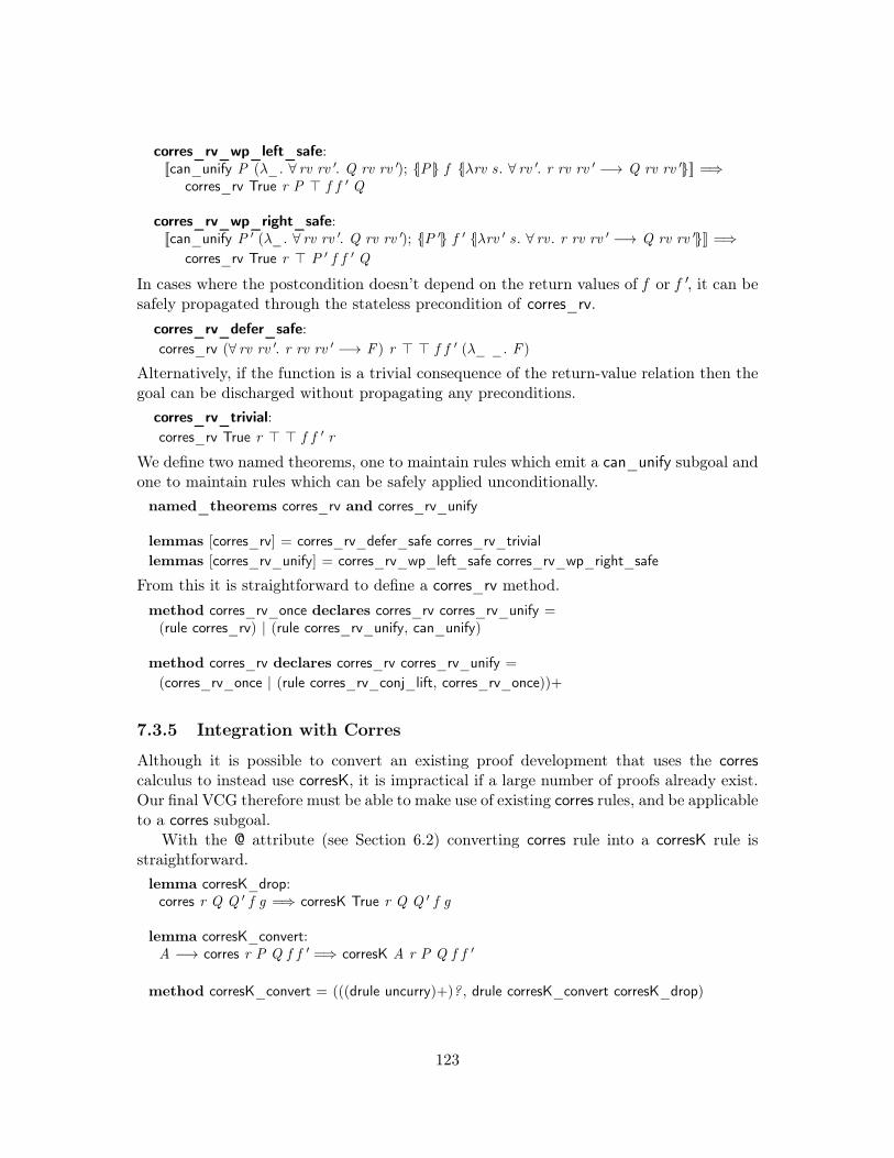
corres_rv_wp_left_safe:[[can_unify P (λ_. ∀ rv rv ′. Q rv rv ′); {|P |} f {|λrv s. ∀ rv ′. r rv rv ′ −→ Q rv rv ′|}]] =⇒

corres_rv True r P > f f ′ Q

corres_rv_wp_right_safe:[[can_unify P ′ (λ_. ∀ rv rv ′. Q rv rv ′); {|P ′|} f ′ {|λrv ′ s. ∀ rv . r rv rv ′ −→ Q rv rv ′|}]] =⇒

corres_rv True r > P ′ f f ′ Q

In cases where the postcondition doesn’t depend on the return values of f or f ′, it can besafely propagated through the stateless precondition of corres_rv.

corres_rv_defer_safe:corres_rv (∀ rv rv ′. r rv rv ′ −→ F ) r > > f f ′ (λ_ _. F )

Alternatively, if the function is a trivial consequence of the return-value relation then thegoal can be discharged without propagating any preconditions.

corres_rv_trivial:corres_rv True r > > f f ′ r

We define two named theorems, one to maintain rules which emit a can_unify subgoal andone to maintain rules which can be safely applied unconditionally.named_theorems corres_rv and corres_rv_unify

lemmas [corres_rv] = corres_rv_defer_safe corres_rv_triviallemmas [corres_rv_unify] = corres_rv_wp_left_safe corres_rv_wp_right_safe

From this it is straightforward to define a corres_rv method.method corres_rv_once declares corres_rv corres_rv_unify =(rule corres_rv) | (rule corres_rv_unify, can_unify)

method corres_rv declares corres_rv corres_rv_unify =

(corres_rv_once | (rule corres_rv_conj_lift, corres_rv_once))+

7.3.5 Integration with Corres

Although it is possible to convert an existing proof development that uses the correscalculus to instead use corresK, it is impractical if a large number of proofs already exist.Our final VCG therefore must be able to make use of existing corres rules, and be applicableto a corres subgoal.

With the @ attribute (see Section 6.2) converting corres rule into a corresK rule isstraightforward.lemma corresK_drop:corres r Q Q ′ f g =⇒ corresK True r Q Q ′ f g

lemma corresK_convert:A −→ corres r P Q f f ′ =⇒ corresK A r P Q f f ′

method corresK_convert = (((drule uncurry)+)? , drule corresK_convert corresK_drop)

123

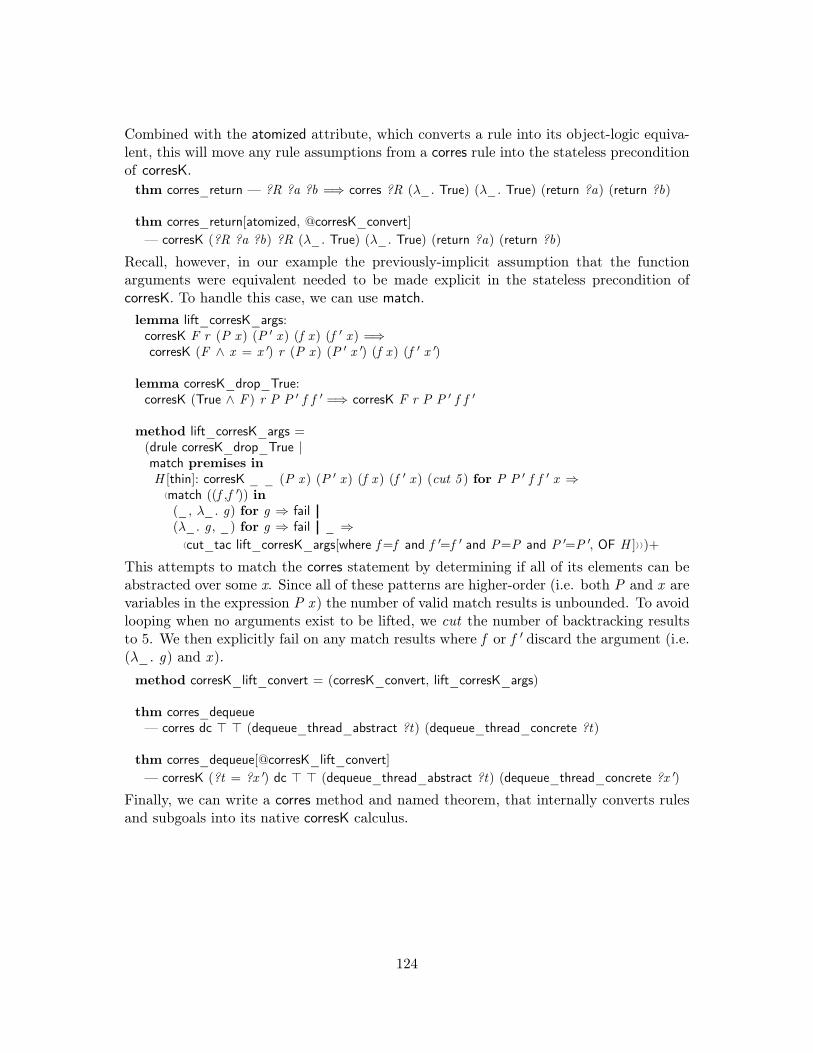
Combined with the atomized attribute, which converts a rule into its object-logic equiva-lent, this will move any rule assumptions from a corres rule into the stateless preconditionof corresK.thm corres_return — ?R ?a ?b =⇒ corres ?R (λ_. True) (λ_. True) (return ?a) (return ?b)

thm corres_return[atomized, @corresK_convert]— corresK (?R ?a ?b) ?R (λ_. True) (λ_. True) (return ?a) (return ?b)

Recall, however, in our example the previously-implicit assumption that the functionarguments were equivalent needed to be made explicit in the stateless precondition ofcorresK. To handle this case, we can use match.lemma lift_corresK_args:corresK F r (P x ) (P ′ x ) (f x ) (f ′ x ) =⇒corresK (F ∧ x = x ′) r (P x ) (P ′ x ′) (f x ) (f ′ x ′)

lemma corresK_drop_True:corresK (True ∧ F ) r P P ′ f f ′ =⇒ corresK F r P P ′ f f ′

method lift_corresK_args =(drule corresK_drop_True |match premises inH [thin]: corresK _ _ (P x ) (P ′ x ) (f x ) (f ′ x ) (cut 5 ) for P P ′ f f ′ x ⇒

〈match ((f ,f ′)) in(_, λ_. g) for g ⇒ fail(λ_. g , _) for g ⇒ fail _ ⇒

〈cut_tac lift_corresK_args[where f=f and f ′=f ′ and P=P and P ′=P ′, OF H ]〉〉)+

This attempts to match the corres statement by determining if all of its elements can beabstracted over some x. Since all of these patterns are higher-order (i.e. both P and x arevariables in the expression P x ) the number of valid match results is unbounded. To avoidlooping when no arguments exist to be lifted, we cut the number of backtracking resultsto 5. We then explicitly fail on any match results where f or f ′ discard the argument (i.e.(λ_. g) and x ).

method corresK_lift_convert = (corresK_convert, lift_corresK_args)

thm corres_dequeue— corres dc > > (dequeue_thread_abstract ?t) (dequeue_thread_concrete ?t)

thm corres_dequeue[@corresK_lift_convert]— corresK (?t = ?x ′) dc > > (dequeue_thread_abstract ?t) (dequeue_thread_concrete ?x ′)

Finally, we can write a corres method and named theorem, that internally converts rulesand subgoals into its native corresK calculus.

124

lemma corresK_start:corresK True r P P ′ a c =⇒ corres r P P ′ a c

named_theorems corres

method corres declares corresK corresK_calc corres =((rule corresK_start)? , corresK corresK : corres[atomized, @corresK_lift_convert])

7.3.6 Corressimp

By decomposing the automation strategy for corres into multiple components, we havethe ability to carefully apply these specialized methods in order to observe and controltheir individual behaviour on proofs, and integrate them into other tools. In many cases,however, the proof author will simply wish to attempt all known strategies in order tomaximally leverage the available automation.

We can integrate this into a single corressimp method, that applies our corres methodsalong with simp and wp repeatedly to the first subgoal. Note that corresK_search isguarded with a match to ensure it is not attempted when no search fact is given.method corressimp uses search wp simp declares corres corresK corresK_calc =((corres| corres_rv| match search in _ ⇒ 〈corresK_search search: search〉

| wp add : wp| simp add : simp)+)[1]

7.4 Application to L4.verified

The methods developed in the previous section are a simplification of their final imple-mentation in L4.verified. In practice, there are many side conditions that have to beconsidered in order to have a robust method that can integrate with existing proofs. Thefinal implementation, including auxiliary methods and the corresK calculus, is approxi-mately 922 lines of Isabelle source: 32 Eisbach methods spanning 121 lines, 36 lines ofML2, 14 definitions spanning 32 lines, and 135 lemmas spanning 733 lines.

Development began by identifying several corres proofs from the L4.verified refinementproof that were excessively manual as a result of the corres calculus. The goal was tobe able to refactor the proofs in-place to use an automated method, without requiringsignificant modifications to the surrounding proofs or rules.

The implementation progressed iteratively, with naive implementations for the coremethods that gradually grew more complex as more side conditions were encounteredwhen the corres proof method was used in more proofs. The majority of the complexity inthe implementation resulted from handling mismatched function bodies and the corres_rvobligations that emerged in those proofs.

2This is a single ML function to retrieve splitting rules for case statements over inductive datatypes,and has been lifted into a standalone rule attribute.

125

To evaluate the method, 9 individual proofs from L4.verified were refactored to usethe corres proof method. In Table 7.1 we show the number of lines of proof for eachlemma before and after it is refactored. The total number of proof lines was reduced 45%,from 475 to 261, with an average reduction of 21 lines and 45% per proof. Some proofshad much more dramatic changes in relative proof size than others, for example set_epwas reduced by almost 80% after refactoring, while resolve_address_bits was only reducedby 24%. This is largely explained by differences in the complexity of the verificationconditions that appear in the proofs. In resolve_address_bits, for example, the proof textis primarily dedicated to solving the verification condition, thus the benefit of the corresmethod is not significant when viewed as a percentage of the total proof size.

In addition to measuring the total reduction in proof size, we can also consider thenumber of corres lemmas that appear in the proof text itself. Each lemma that is explicitlyused indicates a place where the proof author needed to stop to think about the underlyingcalculus, and potentially look up the relevant rule. Learning the library of corres rules hasproven to be a major hurdle when on-boarding new proof engineers, and it is preciselythis manual burden that the corres method aims to alleviate.

In Table 7.2 we show instead the number of corres lemmas that were explicitly used inthe source proof text before and after each proof was refactored. Nearly all corres lemmasno longer appear in the proof text, and the few that remain are either simple terminalrules used to guide corres_search or induction rules used to manually instantiate loopinvariants, and cannot be automatically applied.

There is little to no change in the overall proof processing time for the refactoredproofs, as this is still largely dominated by solving the final verification condition.

7.4.1 Proof Example

To understand the effect of the corres method, and indeed proof automation in general,we show the original 38 line proof of set_asid_pool_corres in Figure 7.3. After the initialuse of 4 corres rules, the rest of the proof is dedicated to solving the emerging verificationconditions. At this point there are 15 open subgoals, with Hoare logic obligations inter-leaved with verification conditions, as seen by the combined used of wp and auto. Clearlythere is some repeated reasoning, as many of the clarsimp, simp and auto lines look verysimilar, but the subgoal structure makes this extremely difficult to capture or exploit.

After the proof has been refactored, it is much more straightforward.lemma set_asid_pool_corres:a = inv ASIDPool a ′ o ucast =⇒corres dc (asid_pool_at p and valid_etcbs) (asid_pool_at ′ p)

(set_asid_pool p a) (setObject p a ′)unfolding set_asid_pool_defapply (corressimp search: set_other_obj_corres[where P=λ_. True]

wp: get_object_ret get_object_wp)apply (clarsimp simp: obj_at_simps other_obj_relation_def asid_pool_relation_def )by (auto simp: obj_at_simps typ_at_to_obj_at_arches

split : Structures_A.kernel_object.splits if_splits arch_kernel_obj.splits)

In this case, corressimp has successfully handled the corres proof obligation and emitted a

126

Table 7.1: Sizes of L4.verified corres proofs before and after refactoring, measured in linesof proof.

Function Name Original Refactored # %Size Size Reduction Reduction

create_mapping_entries 36 17 19 53set_asid_pool 38 10 28 74lookup_pt_slot 24 13 11 46

copy_global_mappings 47 20 27 57find_pd_for_asid 74 55 19 26

getSlotCap 14 11 3 21resolve_address_bits 156 119 37 24

set_ep 33 7 26 79set_ntfn 32 8 24 75Total 454 260 194 43

Average 50 29 21 51

Table 7.2: Number of corres lemmas appearing in proof text of L4.verified corres proofsbefore and after refactoring.

Function Name Original Refactored # %# Lemmas # Lemmas Reduction Reduction

create_mapping_entries 12 0 12 100set_asid_pool 4 1 3 75lookup_pt_slot 4 0 4 100

copy_global_mappings 9 1 8 89find_pd_for_asid 7 2 5 71

getSlotCap 4 0 4 100resolve_address_bits 6 1 5 83

set_ep 4 1 3 75set_ntfn 3 1 2 67Total 53 7 46 87

Average 6 1 9 84

127

lemma set_asid_pool_corres:a = inv ASIDPool a ′ o ucast =⇒corres dc (asid_pool_at p and valid_etcbs) (asid_pool_at ′ p)

(set_asid_pool p a) (setObject p a ′)apply (simp add : set_asid_pool_def)apply (rule corres_symb_exec_l)apply (rule corres_symb_exec_l)apply (rule corres_guard_imp)apply (rule set_other_obj_corres [where P=λko::asidpool. True])

apply simpapply (clarsimp simp: obj_at ′_def projectKOs)apply (erule map_to_ctes_upd_other, simp, simp)apply (simp add : a_type_def is_other_obj_relation_type_def)apply (simp add : objBits_simps archObjSize_def)apply simpapply (simp add : objBits_simps archObjSize_def pageBits_def)apply (simp add : other_obj_relation_def asid_pool_relation_def)apply assumptionapply (simp add : typ_at ′_def obj_at ′_def ko_wp_at ′_def projectKOs)apply clarsimpapply (case_tac ko; simp)apply (rename_tac arch_kernel_object)apply (case_tac arch_kernel_object ; simp)prefer 5apply (rule get_object_sp)

apply (clarsimp simp: obj_at_def exs_valid_def assert_def a_type_def return_def fail_def)apply (auto split : Structures_A.kernel_object.split_asm arch_kernel_obj.split_asm if_split_asm)[1]apply wpapply (clarsimp simp: obj_at_def a_type_def)apply (auto split : Structures_A.kernel_object.split_asm arch_kernel_obj.split_asm if_split_asm)[1]apply (rule no_fail_pre, wp)apply (clarsimp simp: simp: obj_at_def a_type_def)apply (auto split : Structures_A.kernel_object.splits arch_kernel_obj.splits if_split_asm)[1]apply (clarsimp simp: obj_at_def exs_valid_def get_object_def exec_gets)apply (simp add : return_def)apply (rule no_fail_pre, wp)apply (clarsimp simp add : obj_at_def)done

Figure 7.3: The corres proof for set_asid_pool before refactoring.

128

single verification condition. Although the corressimp method has only directly replaced4 uses of the corres rules, it has additionally produced a subgoal structure which is muchmore amenable to using Isabelle’s built-in automation. Previously, verification conditionswere interleaved with Hoare logic obligations, and many related and similar conditionshad been spread across multiple subgoals.

In the refactored proof, the single verification condition can now be handled with oneinvocation of auto (and some help from clarsimp). This has effectively factored out asignificant amount of duplicated reasoning from the original proof, while also abstractingaway the details of the corres calculus.

As the development of L4.verified continues, the corres method has now started toappear in new proofs.

7.5 Conclusion

In this chapter we have outlined the design and implementation of a new proof method forhandling refinement proofs using Eisbach. This was motivated by identifying a significantsource of manual proof effort in L4.verified. Although the Hoare logic verification-conditiongenerator (VCG) wp has been used extensively in the L4.verified proofs, no such VCGexisted for automating refinement proofs.

Building on the corres calculus [23], we identified a key factor that made it unsuitableto effectively use automated reasoning. This motivated the development of a new corresKcalculus, which enabled greater control over how verification conditions were propagatedthrough Isabelle’s subgoal structure. With this, we were able to build a corresK methodfor automating corresK proofs, and ultimately integrate this into the existing corres infras-tructure of L4.verified in a corres method.

We refactored several existing refinement proofs from L4.verified to use this new proofmethod, achieving a significant reduction in overall proof size in many cases, and in everycase eliminating most of the corres calculus rules that appear in the final proof text. Thebenefit of the corres method is therefore twofold: explicit use of corres rules is no longerrequired except when completely necessary, reducing the manual burden of generatinga verification condition; and the resulting condition is now a single subgoal, enablingmuch more effective use of Isabelle’s built-in automation (or domain-specific methods)and avoiding duplicated reasoning in the proof text.

This case study motivated and made use of the advanced features presented in Chap-ter 6. An initial design goal for this VCG was for the majority of the source to be Isar andEisbach, with as little as possible ML. Where ML functionality was initially required,general-purpose tools were often built instead (i.e. the @ attribute and fold_subgoalsmethod). The apply_debug command was designed to trace the backtracking behaviourof corresK_search, and was later updated to support proof state modifications in order toperform ad-hoc experiments with different corresK calculational rules. The final result ofthis study was both an effective corres proof method, and a rich library of tools for futuremethod development.

Developing the corresK calculus was necessary due to the original focus of the correscalculus on manual, interactive proofs. It is a conservative extension of corres that provides

129

a minimal extra layer in order to support the necessary formal bookkeeping for a VCG.Were Eisbach available during the initial development of corres, it is highly likely thata VCG would have been developed in tandem with the calculus itself and the resultswould have been much different. For example, annotated specifications could have beengenerated from the invariant proofs and avoided the need for Hoare logic reasoning in themiddle of each corres proof.

Eisbach allows such experiments to be carried out easily, allowing for more informeddecisions when embarking on new proof developments.

130

Chapter 8

Conclusion

The demand for software verification is growing [28]: as complex computer systems areentrusted with an ever-increasing range of mission-critical tasks, their correctness andresilience to attack is paramount. In the past few decades, interactive theorem provers(ITPs) have increased the practical scope of using formal logic to prove the correctnessof software. Large-scale verification projects, such as L4.verified, are now becoming morecommon-place. L4.verified consists of over 500,000 lines of Isabelle proof text, verifyingseL4’s relatively small 10,000 line C implementation.

In Section 2.3 we introduced proof engineering as the practice of managing the scal-ability issues inherent to producing and maintaining large proofs in ITPs. Effectivelyengineering a proof requires productively using (or building) frameworks in order to mini-mize the cost of both its initial development and ongoing maintenance. A critical aspect ofproof engineering is performing empirical analysis of proof projects and artefacts, in orderto inform cost and effort models of formal proof development. We discussed a researchagenda by Jeffery et al. [39], in which they identify over thirty open questions in proofengineering that require additional data. In this thesis, we noted this question from theagenda:

How are characteristics of formal specifications, properties, or code related toeffort in formal proofs?

We considered this question in Chapter 4 by building on previous work by Staples etal. [64][65], where they establish a linear relationship between proof effort and proof size,as well as between code size and formal specification size. In our study, we developedmetrics to investigate the relationship between the size of a formal statement and the sizeof its proof, finding a quadratic relationship in the verification projects considered. Thissuggests, combined with the results from Staples et al., that with current methods theeffort required to prove the correctness of software will increase quadratically with codesize.

This quadratic scaling factor poses a significant challenge for formal verification oflarger software systems. It indicates that hundreds of thousands of lines of verified codepotentially results in tens of millions of lines of proof, requiring dozens of person-years tocomplete.

131

Motivated by this, we considered a second question from the research agenda:

How can we best combine interactive proof and proof automation to achievehigh proof productivity during initial proof development and subsequent proofmaintenance?

The availability and use of automated reasoning is intrinsically linked with the scala-bility of proof effort. In an interactive theorem prover, each line of proof indicates someupper bound on the amount of reasoning that can be expressed with a single step. Mostmodern ITPs provide a tactic language for writing new proof tactics, either as a domain-specific language (e.g. Ltac in Coq), or a set of standard libraries in the implementationlanguage of the prover (e.g. ML in HOL).

In Isabelle, powerful automated proof methods come built-in with Isar. This has al-lowed for significant results to be achieved without requiring a specialized language fordeveloping new methods, as custom proof methods can be implemented in ML by expertusers. However, larger proof developments have seen scalability and maintenance chal-lenges arise from a lack of custom proof methods. We hypothesized that this was due to alack of familiarity with ML within the Isabelle community. Although many proofs wouldbenefit from custom proof methods, they can still be completed without them, at the costof duplicated reasoning in the proof text or additional manual effort.

To address this, in Chapter 5 we presented Eisbach, a proof method language and exten-sible proof automation framework for Isabelle that leverages Isar’s syntax and integrationwith ML. Eisbach’s expressive match method uses Isabelle’s unifier to give control-flow toinner method expressions, while using subgoal focusing to provide direct access to logicalelements of Isabelle’s subgoal state. Although match is a core aspect of Eisbach, it is im-plemented in ML as a standard proof method with no special status. This is a testamentto the extensibility of Eisbach, as similarly expressive language extensions can easily beprovided by end users. This is explored further in Chapter 6 where we introduced a suiteof language extensions, including tools to treat proof methods as fact-producing functions,as well as an interactive debugger.

Eisbach’s integration with named theorems additionally allows for ad-hoc extensibility,where proof methods can refer to named collections of facts that are dynamically extendedlater. This functionality is critical in the proof methods introduced in Chapter 7 to reducethe manual effort of proofs in L4.verified. Using this, as well as extensions presentedin Chapter 6, we developed a set of proof methods for calculating verification conditionsin refinement proofs. By applying these methods to several existing proofs from L4.verified,we demonstrated that their size and complexity could be drastically reduced. Across 9lemmas we reduced proof size by 21-77%, with an average reduction of 51%. Additionally,we reduced explicit references to refinement calculus rules by 67-100%, with an averagereduction of 84%.

These results are a promising indication that powerful automated methods can addressthe quadratic scaling factor identified in Chapter 4. By reducing the required proof effortfor each individual instance of a particular problem, we hypothesize that we can reducethe coefficient on this quadratic relationship and, in some cases, reduce it to linear. Inthe presence of automation, however, even measuring proof effort becomes more complex

132

as the role of the proof author shifts from providing individual proof steps to simplyguiding automated methods. Each method will therefore likely require its own model forunderstanding how much effort is required for a proof author to determine the necessaryinput parameters.

Eisbach has been incorporated into many other proof developments since its initial2015 release, confirming our experience that Eisbach can make proof development moreproductive. In his PhD thesis [9], Alasdair Armstrong remarks “compared to the develop-ment of tactics in Isabelle/ML. . . Eisbach makes the development of such tactics availableto even the novice Isabelle user.”

Building trustworthy, verified systems is crucial for the increasing number of mission-critical applications of computers. As larger, more complex software systems are beingformally verified in interactive theorem provers, the discipline of proof engineering is be-coming more important. A proof engineer requires both the tools and knowledge to managethe challenges, costs and efforts inherent in developing and maintaining large-scale proofs.

In this thesis, we have presented Eisbach as a supporting framework for scalable proofengineering in Isabelle, motivated by an empirical investigation and evaluated with a casestudy. By increasing the accessibility of writing custom proof automation with Eisbach, wecan achieve better scalability of proof efforts. This enables the field of proof engineering totackle future grand verification challenges, expanding our capacity to verify larger mission-critical systems.

133

Bibliography

[1] Afp statistics. https://www.isa-afp.org/statistics.html. [Online; accessed2018-03-23].

[2] Coq package index. https://coq.inria.fr/opam/www/. [Online; accessed 2018-03-23].

[3] Deploy: Industrial deployment of system engineering methods providing high de-pendability and productivity. http://www.deploy-project.eu/. [Online; accessed2015-02-06].

[4] Mizar mathematical library. http://mizar.org/library/. [Online; accessed 2018-03-23].

[5] sel4/l4v: Proofs for sel4-8.0.0. https://doi.org/10.5281/zenodo.1168016, Feb.2018. [Online; accessed 2018-04-15].

[6] Alama, J., Mamane, L., and Urban, J. Dependencies in formal mathematics:Applications and extraction for Coq and Mizar. In Intelligent Computer Mathematics(2012), pp. 1–16.

[7] Alkassar, E., Paul, W., Starostin, A., and Tsyban, A. Pervasive verificationof an OS microkernel. In Verified Software: Theories, Tools, Experiments (2010),pp. 71–85.

[8] Andronick, J., Jeffery, R., Klein, G., Kolanski, R., Staples, M., Zhang,H. J., and Zhu, L. Large-scale formal verification in practice: A process perspec-tive. In International Conference on Software Engineering (Zurich, Switzerland, June2012), ACM, pp. 1002–1011.

[9] Armstrong, A. Formal Analysis of Concurrent Programs. PhD thesis, Universityof Sheffield, 2015.

[10] Ballarin, C. Locales and locale expressions in Isabelle/Isar. In Types for Proofsand Programs (TYPES 2003) (2003), S. Berardi, M. Coppo, and F. Damiani, Eds.,vol. 3085 of Lecture Notes in Computer Science, Springer.

[11] Ballarin, C. Locales: A module system for mathematical theories. Journal ofAutomated Reasoning 52, 2 (2014), 123–153.

134

[12] Bancerek, G., and Rudnicki, P. Information retrieval in MML. In InternationalConference on Mathematical Knowledge Management (2003), Springer, pp. 119–132.

[13] Barendregt, H., and Wiedijk, F. The challenge of computer mathematics. Philo-sophical Transactions of the Royal Society of London A: Mathematical, Physical andEngineering Sciences 363, 1835 (2005), 2351–2375.

[14] Bellard, F. Qemu, a fast and portable dynamic translator. In Proceedings of theAnnual Conference on USENIX Annual Technical Conference (Berkeley, CA, USA,2005), ATEC ’05, USENIX Association, pp. 41–41.

[15] Berghofer, S., and Nipkow, T. Proof terms for simply typed higher order logic.In Theorem Proving in Higher Order Logics, M. Aagaard and J. Harrison, Eds.,vol. 1869 of Lecture Notes in Computer Science. Springer Berlin Heidelberg, 2000,pp. 38–52.

[16] Bollin, A. Metrics for quantifying evolutionary changes in Z specifications. Journalof Software: Evolution and Process 25, 9 (2013), 1027–1059.

[17] Bourke, T., Daum, M., Klein, G., and Kolanski, R. Challenges and experi-ences in managing large-scale proofs. In Intelligent Computer Mathematics (2012),pp. 32–48.

[18] Boyer, R., and Moore, J. A Computational Logic. Academic Press, 1979.

[19] Boyton, A., Andronick, J., Bannister, C., Fernandez, M., Gao, X.,Greenaway, D., Klein, G., Lewis, C., and Sewell, T. Formally verified systeminitialisation. In Proceedings of the 15th International Conference on Formal Engi-neering Methods (Queenstown, New Zealand, Oct. 2013), Lindsay Groves, Jing Sun,Ed., Springer, pp. 70–85.

[20] Checkoway, S., McCoy, D., Kantor, B., Anderson, D., Shacham, H., Sav-age, S., Koscher, K., Czeskis, A., Roesner, F., and Kohno, T. Comprehen-sive experimental analyses of automotive attack surfaces. In Proceedings of the 20thUSENIX Security Symposium (2011).

[21] Chlipala, A. Mostly-automated verification of low-level programs in computationalseparation logic. ACM SIGPLAN Notices 46, 6 (Jun 2011), 234.

[22] Chrząszcz, J. Implementing modules in the coq system. In International Conferenceon Theorem Proving in Higher Order Logics (2003), Springer, pp. 270–286.

[23] Cock, D., Klein, G., and Sewell, T. Secure microkernels, state monads andscalable refinement. In Proceedings of the 21st International Conference on Theo-rem Proving in Higher Order Logics (Montreal, Canada, Aug. 2008), Otmane AitMohamed, César Muñoz, Sofiène Tahar, Ed., Springer, pp. 167–182.

[24] de Moura, L., Kong, S., Avigad, J., Van Doorn, F., and von Raumer,J. The lean theorem prover (system description). In International Conference onAutomated Deduction (2015), Springer, pp. 378–388.

135

[25] Delahaye, D. A tactic language for the system Coq. In International Conference onLogic for Programming, Artificial Intelligence and Reasoning (Nov. 2000), vol. 1955of Lecture Notes in Computer Science, Springer.

[26] Dijkstra, E. W. Guarded commands, nondeterminacy and formal derivation ofprograms. Commun. ACM 18, 8 (Aug. 1975), 453–457.

[27] Felty, A., and Howe, D. Generalization and reuse of tactic proofs. Logic Pro-gramming and Automated Reasoning (1994).

[28] Fisher, K. HACMS: High assurance cyber military systems. In Proceedings ofthe 2012 ACM Conference on High Integrity Language Technology (Boston, Mas-sachusetts, USA, 2012), HILT ’12, ACM, pp. 51–52.

[29] Fowler, M., Beck, K., Brant, J., Opdyke, W., and Roberts, D. Refactoring:improving the design of existing code. Addison-Wesley Professional, 1999.

[30] Gonthier, G., and Mahboubi, A. An introduction to small scale reflection inCoq. J. Formalized Reasoning 3, 2 (2010).

[31] Gonthier, G., Ziliani, B., Nanevski, A., and Dreyer, D. How to make adhoc proof automation less ad hoc. J. Funct. Program. 23, 4 (2013), 357–401.

[32] Gordon, M. J. C., Milner, R., and Wadsworth, C. P. Edinburgh LCF: AMechanized Logic of Computation. LNCS 78. Springer, 1979.

[33] Greenaway, D. Automated Proof-Producing Abstraction of C Code. PhD thesis,Sydney, Australia, jan 2015.

[34] Grov, G., and Maclean, E. Towards automated proof strategy generalisation.CoRR abs/1303.2 (2013), 1–15.

[35] Halperin, D., Clark, S. S., Fu, K., Heydt-Benjamin, T. S., Defend, B.,Kohno, T., Ransford, B., Morgan, W., and Maisel, W. H. Pacemakers andimplantable cardiac defibrillators: Software radio attacks and zero-power defenses. InProceedings of the IEEE Symposium on Security and Privacy (Oakland, CA, USA,May 2008), pp. 129–142.

[36] Halstead, M. H. Elements of Software Science (Operating and Programming Sys-tems Series). Elsevier Science Inc., New York, NY, USA, 1977.

[37] Hupel, L. Interactive simplifier tracing and debugging in Isabelle. In IntelligentComputer Mathematics. Springer, 2014, pp. 328–343.

[38] ISO/IEC 19761:2011, Software engineering – COSMIC: a functional size measure-ment method , 2011.

[39] Jeffery, R., Staples, M., Andronick, J., Klein, G., and Murray, T. An em-pirical research agenda for understanding formal methods productivity. Informationand Software Technology 60 (2015), 102–112.

136

[40] Kaufmann, M., and Moore, J. S. ACL2: An industrial strength version of Nqthm.In Computer Assurance (1996).

[41] Klein, G., Andronick, J., Elphinstone, K., Murray, T., Sewell, T.,Kolanski, R., and Heiser, G. Comprehensive formal verification of an OS micro-kernel. ACM Transactions on Computer Systems 32, 1 (Feb. 2014), 2:1–2:70.

[42] Klein, G., Elphinstone, K., Heiser, G., Andronick, J., Cock, D., Derrin,P., Elkaduwe, D., Engelhardt, K., Kolanski, R., Norrish, M., Sewell,T., Tuch, H., and Winwood, S. seL4: Formal verification of an OS kernel. InACM Symposium on Operating Systems Principles (Big Sky, MT, USA, Oct. 2009),ACM, pp. 207–220.

[43] Klein, G., Nipkow, T., and Paulson, L. The archive of formal proofs. http://afp.sf.net. [Online; accessed 2018-03-28].

[44] Lochbihler, A. Jinja with threads. Archive of Formal Proofs (Dec. 2007). http://afp.sf.net/entries/JinjaThreads.shtml, Formal proof development [Online;accessed 2018-04-15].

[45] Maric, F. Formal verification of modern SAT solvers. Archive of Formal Proofs (July2008). http://afp.sf.net/entries/SATSolverVerification.shtml, Formal proofdevelopment [Online; accessed 2018-04-15].

[46] Matichuk, D., and Murray, T. Extensible specifications for automatic re-use ofspecifications and proofs. In 10th International Conference on Software Engineeringand Formal Methods (Thessaloniki, Greece, Dec. 2012), p. 8.

[47] Matichuk, D., Murray, T., Andronick, J., Jeffery, R., Klein, G., andStaples, M. Empirical study towards a leading indicator for cost of formal softwareverification. In Proceedings of the 37th International Conference on Software Engi-neering - Volume 1 (Piscataway, NJ, USA, 2015), ICSE ’15, IEEE Press, pp. 722–732.

[48] Matichuk, D., Murray, T., and Wenzel, M. Eisbach: A proof method languagefor Isabelle. J. Autom. Reason. 56, 3 (Mar. 2016), 261–282.

[49] Matichuk, D., Wenzel, M., and Murray, T. The Eisbach user manual. https://isabelle.in.tum.de/doc/eisbach.pdf. [Online; accessed 2018-03-23].

[50] Matichuk, D., Wenzel, M., and Murray, T. An Isabelle proof method language.In Interactive Theorem Proving (ITP) (Vienna, Austria, July 2014), p. 16.

[51] McCabe, T. A complexity measure. Software Engineering, IEEE Transactions onSE-2, 4 (Dec 1976), 308–320.

[52] Murray, T., Matichuk, D., Brassil, M., Gammie, P., Bourke, T., Seefried,S., Lewis, C., Gao, X., and Klein, G. seL4: from general purpose to a proofof information flow enforcement. In IEEE Symposium on Security and Privacy (SanFrancisco, CA, May 2013), pp. 415–429.

137

[53] Murray, T., Matichuk, D., Brassil, M., Gammie, P., and Klein, G. Nonin-terference for operating system kernels. In The Second International Conference onCertified Programs and Proofs (Kyoto, Dec. 2012), Chris Hawblitzel and Dale Miller,Ed., Springer, pp. 126–142.

[54] Nipkow, T., Paulson, L., and Wenzel, M. Isabelle/HOL — A Proof Assistantfor Higher-Order Logic, vol. 2283 of Lecture Notes in Computer Science. Springer,2002.

[55] Olszewska (Pląska), M., and Sere, K. Specification metrics for Event-B devel-opments. In Proceedings of the CONQUEST 2010: “Software Quality Improvement”(2010), I. Schieferdecker, R. Seidl, and S. Goericke, Eds., International Software Qual-ity Institute, pp. 1–12.

[56] Paulson, L. C. Isabelle: the next 700 theorem provers. In Logic and ComputerScience, P. Odifreddi, Ed. Academic Press, 1990.

[57] Ringer, T., Yazdani, N., Leo, J., and Grossman, D. Adapting proof automa-tion to adapt proofs. In CPP (2018).

[58] Rudnicki, P. An overview of the Mizar project. In Types for Proofs and Programs(1992), pp. 1–22.

[59] Samson, W. B., Nevill, D. G., and Dugard, P. I. Predictive software metricsbased on a formal specification. Inf. Softw. Technol. 29, 5 (June 1987), 242–248.

[60] Schirmer, N. Verification of sequential imperative programs in Isabelle/HOL. PhDthesis, Technische Universität München, 2006.

[61] Sewell, T. seL4 enforces integrity. Interactive Theorem Proving 6898 (2011), 325–340.

[62] Sewell, T., Myreen, M., and Klein, G. Translation validation for a verifiedOS kernel. In ACM SIGPLAN Conference on Programming Language Design andImplementation (Seattle, Washington, USA, June 2013), ACM, pp. 471–481.

[63] Sewell, T., Winwood, S., Gammie, P., Murray, T., Andronick, J., andKlein, G. seL4 enforces integrity. In Proceedings of the 2nd International Conferenceon Interactive Theorem Proving (Nijmegen, The Netherlands, Aug. 2011), M. C. J. D.van Eekelen, H. Geuvers, J. Schmaltz, and F. Wiedijk, Eds., vol. 6898 of Lecture Notesin Computer Science, Springer, pp. 325–340.

[64] Staples, M., Jeffery, R., Andronick, J., Murray, T., Klein, G., andKolanski, R. Productivity for proof engineering. In Empirical Software Engineeringand Measurement (Turin, Italy, Sept. 2014).

[65] Staples, M., Kolanski, R., Klein, G., Lewis, Corey nd Andronick, J.,Murray, T., Jeffery, R., and Bass, L. Formal specifications better than functionpoints for code sizing. In International Conference on Software Engineering (San

138

Francisco, USA, May 2013), David Notkin, Betty H. C. Cheng, Klaus Pohl, Ed.,IEEE, pp. 1257–1260.

[66] Stidolph, D. C., and Whitehead, J. Managerial issues for the considerationand use of formal methods. In In Stefania Gnesi, Keijiro Araki, and Dino Mandrioli(eds.), FME 2003, International Symposium of Formal Methods Europe (2003), pp. 8–14.

[67] Tabareh, A. Predictive software measures based on formal Z specifications. Master’sthesis, University of Gothenburg - Department of Computer Science and Engineering,2011.

[68] Trustworthy Systems Team. seL4 proofs for API 1.03, release 2014-08-10, Aug2014.

[69] Tuch, H., Klein, G., and Norrish, M. Types, bytes, and separation logic. InACM SIGPLAN Notices (2007), vol. 42, ACM, pp. 97–108.

[70] Wenzel, M. Isar - a generic interpretative approach to readable formal proof doc-uments. In Proceedings of the 12th International Conference on Theorem Provingin Higher Order Logics (London, UK, UK, 1999), TPHOLs ’99, Springer-Verlag,pp. 167–184.

[71] Wenzel, M. Isabelle/Isar—a versatile environment for human-readable formal proofdocuments. PhD thesis, Technische Universität München, 2002.

[72] Wenzel, M., and Chaieb, A. SML with antiquotations embedded intoIsabelle/Isar. In Workshop on Programming Languages for Mechanized Mathematics(PLMMS 2007). Hagenberg, Austria (June 2007), J. Carette and F. Wiedijk, Eds.

[73] Wenzel, M., and Wiedijk, F. A comparison of Mizar and Isar. Journal ofAutomated Reasoning 29, 3-4 (2002), 389–411.

[74] Whiteside, I., Aspinall, D., Dixon, L., and Grov, G. Towards formal proofscript refactoring. In Intelligent Computer Mathematics (2011), pp. 260–275.

[75] Wiedijk, F., Ed. The Seventeen Provers of the World, vol. 3600. 2006.

[76] Ziliani, B., Dreyer, D., Krishnaswami, N. R., Nanevski, A., and Vafeiadis,V. Mtac: a monad for typed tactic programming in Coq. In ICFP (2013), G. Mor-risett and T. Uustalu, Eds., ACM.

139