automatically locating sensor position on an e-textile
TRANSCRIPT

Automatically Locating Sensor Position on an E-textileGarment Via Pattern Recognition
by
Andrew R. Love
Thesis submitted to the Faculty of the
Virginia Polytechnic Institute and State University
in partial fulfillment of the requirements for the degree of
Master of Science
in
Computer Engineering
Dr. Thomas L. Martin, Chair
Dr. Mark T. Jones, Co-Chair
Dr. Peter M. Athanas
September 30, 2009
Blacksburg, Virginia
Keywords: E-Textiles, Singular Value Decomposition
Copyright 2009, Andrew R. Love

Automatically Locating Sensor Position on an E-textile Garment Via
Pattern Recognition
Andrew R. Love
(ABSTRACT)
Electronic textiles are a sound platform for wearable computing. Many applications have
been devised that use sensors placed on these textiles for fields such as medical monitoring and
military use or for display purposes. Most of these applications require that the sensors have
known locations for accurate results. Activity recognition is one application that is highly
dependent on knowledge of the sensor position. Therefore, this thesis presents the design
and implementation of a method whereby the location of the sensors on the electronic textile
garments can be automatically identified when the user is performing an appropriate activity.
The software design incorporates principle component analysis using singular value decom-
position to identify the location of the sensors. This thesis presents a method to overcome
the problem of bilateral symmetry through sensor connector design and sensor orientation
detection. The scalability of the solution is maintained through the use of culling techniques.
This thesis presents a flexible solution that allows for the fine-tuning of the accuracy of the
results versus the number of valid queries, depending on the constraints of the application.
The resulting algorithm is successfully tested on both motion capture and sensor data from
an electronic textile garment.

Contents
1 Introduction 1
1.1 Motivation . . . . . . . . . . . . . . . . . . . . . . . . . . . . . . . . . . . . . 2
1.2 Contributions . . . . . . . . . . . . . . . . . . . . . . . . . . . . . . . . . . . 3
1.3 Thesis Organization . . . . . . . . . . . . . . . . . . . . . . . . . . . . . . . . 4
2 Background 5
2.1 Electronic Textiles . . . . . . . . . . . . . . . . . . . . . . . . . . . . . . . . 6
2.2 Related Work . . . . . . . . . . . . . . . . . . . . . . . . . . . . . . . . . . . 8
2.3 Prior Work - E-textile Pants . . . . . . . . . . . . . . . . . . . . . . . . . . . 9
2.3.1 E-textile Pants Orientation . . . . . . . . . . . . . . . . . . . . . . . . 9
2.3.2 E-textile Pants Applications . . . . . . . . . . . . . . . . . . . . . . . 10
2.4 Prior Work - E-textile Jumpsuit . . . . . . . . . . . . . . . . . . . . . . . . . 12
2.4.1 E-textile Jumpsuit Orientation . . . . . . . . . . . . . . . . . . . . . 13
2.4.2 Pendulum Model . . . . . . . . . . . . . . . . . . . . . . . . . . . . . 14
iii

3 Algorithm 17
3.1 Algorithm Considerations . . . . . . . . . . . . . . . . . . . . . . . . . . . . 19
3.2 Orientation . . . . . . . . . . . . . . . . . . . . . . . . . . . . . . . . . . . . 20
3.3 Singular Value Decomposition Analysis . . . . . . . . . . . . . . . . . . . . . 30
3.3.1 Singular Value Decomposition . . . . . . . . . . . . . . . . . . . . . . 30
3.3.2 Principle Component Analysis . . . . . . . . . . . . . . . . . . . . . . 31
3.3.3 k Selection . . . . . . . . . . . . . . . . . . . . . . . . . . . . . . . . . 31
3.3.4 Applying SVD and PCA . . . . . . . . . . . . . . . . . . . . . . . . . 32
3.4 Matching Algorithm And Optimization . . . . . . . . . . . . . . . . . . . . . 35
3.4.1 Training Selection and Culling . . . . . . . . . . . . . . . . . . . . . . 35
3.4.2 Matching Algorithm . . . . . . . . . . . . . . . . . . . . . . . . . . . 40
4 Results 43
4.1 Experimental Setup . . . . . . . . . . . . . . . . . . . . . . . . . . . . . . . . 44
4.2 Experimental Procedure . . . . . . . . . . . . . . . . . . . . . . . . . . . . . 48
4.3 Threshold Testing . . . . . . . . . . . . . . . . . . . . . . . . . . . . . . . . . 50
4.4 Sample Size Testing . . . . . . . . . . . . . . . . . . . . . . . . . . . . . . . . 51
4.5 Ameliorating Errors . . . . . . . . . . . . . . . . . . . . . . . . . . . . . . . . 52
4.6 Per Training Set and Per Subject Testing . . . . . . . . . . . . . . . . . . . . 55
4.7 Algorithm Testing . . . . . . . . . . . . . . . . . . . . . . . . . . . . . . . . . 61
iv

4.7.1 Voting Testing . . . . . . . . . . . . . . . . . . . . . . . . . . . . . . 70
5 Conclusions 76
5.1 Future Work . . . . . . . . . . . . . . . . . . . . . . . . . . . . . . . . . . . . 77
Bibliography 79
v

List of Figures
2.1 Half Meter Pendulum Example . . . . . . . . . . . . . . . . . . . . . . . . . 15
2.2 One Meter Pendulum Example . . . . . . . . . . . . . . . . . . . . . . . . . 16
3.1 Algorithm Flow Chart . . . . . . . . . . . . . . . . . . . . . . . . . . . . . . 18
3.2 Sensor Orientations . . . . . . . . . . . . . . . . . . . . . . . . . . . . . . . . 21
3.3 Jumpsuit . . . . . . . . . . . . . . . . . . . . . . . . . . . . . . . . . . . . . . 25
3.4 Jumpsuit Orientations (g) . . . . . . . . . . . . . . . . . . . . . . . . . . . . 26
3.5 Independent Orientation Stance . . . . . . . . . . . . . . . . . . . . . . . . . 27
3.6 Independent Orientation Stance Model . . . . . . . . . . . . . . . . . . . . . 28
3.7 Preliminary Results . . . . . . . . . . . . . . . . . . . . . . . . . . . . . . . . 39
4.1 Closeup of Fabric and Sensor . . . . . . . . . . . . . . . . . . . . . . . . . . 44
4.2 Sensor Positions on the Jumpsuit . . . . . . . . . . . . . . . . . . . . . . . . 48
4.3 Spearman Correlation of Threshold and Accuracy versus Height . . . . . . . 51
4.4 Walking Data Sample Size Versus Accuracy . . . . . . . . . . . . . . . . . . 52
vi

4.5 80% Accuracy Required Thresholds for Differing Heights . . . . . . . . . . . 54
4.6 64% Accuracy Required Thresholds for Differing Heights . . . . . . . . . . . 55
4.7 Lower Body Training Set Average . . . . . . . . . . . . . . . . . . . . . . . . 58
4.8 Lower Body Using Training Set 8 . . . . . . . . . . . . . . . . . . . . . . . . 58
4.9 Lower Body Using Training Set 1 . . . . . . . . . . . . . . . . . . . . . . . . 59
4.10 Lower Body Subject Average Performance Over All Training Sets . . . . . . 60
4.11 Multiple (1-4) Versus Single (5-8) Subject Training Sets . . . . . . . . . . . . 62
4.12 Histogram of Upper Body Basketball Data . . . . . . . . . . . . . . . . . . . 68
4.13 Summarized Accuracy Versus Threshold Results for the Lower Body . . . . . 69
4.14 Summarized Accuracy Versus Threshold Results for the Upper Body . . . . 69
vii

List of Tables
3.1 S Matrix Example . . . . . . . . . . . . . . . . . . . . . . . . . . . . . . . . 31
3.2 Simplified Matching Algorithm Data Matrix . . . . . . . . . . . . . . . . . . 33
3.3 Example Threshold Accuracy Table . . . . . . . . . . . . . . . . . . . . . . . 38
3.4 Example Threshold Accuracy Percentage . . . . . . . . . . . . . . . . . . . . 38
3.5 Threshold Example . . . . . . . . . . . . . . . . . . . . . . . . . . . . . . . . 41
4.1 Data Format . . . . . . . . . . . . . . . . . . . . . . . . . . . . . . . . . . . 46
4.2 Training Set Numbers . . . . . . . . . . . . . . . . . . . . . . . . . . . . . . 56
4.3 Tukey Test By Subject . . . . . . . . . . . . . . . . . . . . . . . . . . . . . . 56
4.4 Multiple Versus Single Training Set Numbers . . . . . . . . . . . . . . . . . . 61
4.5 Predicted Versus Actual Sensor Position . . . . . . . . . . . . . . . . . . . . 62
4.6 Simulated Walking Jumpsuit Accuracy Versus Threshold . . . . . . . . . . . 64
4.7 Simulated Walking Pants Accuracy Versus Threshold . . . . . . . . . . . . . 65
4.8 Real Walking Pants Accuracy Versus Threshold . . . . . . . . . . . . . . . . 65
4.9 Real Walking Pants Plus Dribbling Accuracy Versus Threshold . . . . . . . . 66
viii

4.10 Simulated Walking Shirt Accuracy Versus Threshold . . . . . . . . . . . . . 66
4.11 Real Walking Shirt Accuracy Versus Threshold . . . . . . . . . . . . . . . . 67
4.12 Lower Body Pacing With Ball Accuracy Versus Threshold . . . . . . . . . . 67
4.13 Real Shirt Basketball Accuracy Versus Threshold . . . . . . . . . . . . . . . 68
4.14 Voting Data Legend . . . . . . . . . . . . . . . . . . . . . . . . . . . . . . . 72
4.15 Real Pants Walking Voting Data . . . . . . . . . . . . . . . . . . . . . . . . 73
4.16 Real Pants Walking Plus Dribbling Voting Data . . . . . . . . . . . . . . . . 74
4.17 Real Shirt Walking Voting Data . . . . . . . . . . . . . . . . . . . . . . . . . 74
4.18 Real Shirt Basketball Voting Data . . . . . . . . . . . . . . . . . . . . . . . . 75
ix

Chapter 1
Introduction
This thesis presents a method whereby the positions of a set of sensors on an electronic
textile (e-textile) garment can be found using pattern recognition while the garment is in
use.
Electronic textile garments are fabrics that include electronics and electrical wiring. These
components are interwoven with the normal yarns to make a seamless whole. These e-textile
garments can have sensors placed throughout the design. Depending on the application,
sensors can be emplaced to detect properties from acceleration and rotation to temperature
and pressure.
The weaving process is performed in much the same way as any other garment. It can be
done by hand or with an automatic loom. The interconnect wiring is chosen such that it
is flexible and of similar thickness to the normal thread. If the electronics are removed or
sealed, the entire garment can be washed just like any other.
1

1.1 Motivation
There are a number of design constraints that motivate the creation of this algorithm. Pre-
vious applications require the knowledge of the location of the sensors to work properly.
Incorporating this data with the sensor placement and design is necessary. Some simple
solutions to discovering the sensor placement must be mentioned to show their drawbacks
for general use.
For the prototype garment described in this thesis, the sensors are connected to the garment
in such a way that they can be removed and replaced. The connection method will be
discussed later in Chapter 4.1. This ease of interchangeability has a cost associated with it.
If the application is attempting to use the garment to perform motion capture [1], than the
position of the sensors will influence the results. This problem is exacerbated by the easily
switchable nature of the sensors, since they could be put back in different locations. In this
case, switching an arm and a leg sensor would have severe consequences in the resulting
motion capture simulation.
Another application that is heavily influenced by the location of the sensors is activity
recognition [2]. Swapping the sensors in this case may change which activity is detected. For
example, kneeling may be recognized as sitting, or vice versa. Therefore, knowing where the
sensors are located is an important component of many e-textile applications.
While there do exist some location independent e-textile applications, such as heart rate
monitoring, this work uses accelerometers, which are heavily location dependent.
One possible solution to discovering the location of the sensor is to add identifying electronics
to the connector. However, the shortcomings of adding IDs at each connector are manyfold.
If the electronics are not waterproof, then washing the garment requires the removal of the
electronics. When the electronics are reconnected to the garment, then care must be taken,
2

as the IDs would still need to be hard coded with the appropriate location. This will cause
mass production to be more difficult, since the ID connectors would not be interchangeable.
Also, having connector IDs will not help if the garment changes. A sensor on the forearm
could move to the elbow if the sleeves are rolled up, and the connector IDs method would
have no way to tell the difference.
One way to determine the sensor’s locations is to program each sensor with its location.
This requires that the sensors are placed in the same location every time. However, with
interchangeable components and a significant number of sensors, this will add considerable
additional work to the setup of the garment. If a part breaks and must be replaced, the new
part needs to be reprogrammed with the appropriate location before it can be used properly.
Another option is to have the user keep track of where each sensor is placed and have some
way to input this data into the application. While this allows for fast placement of the sensors
and easy interchangeability, it adds work for the user. An improvement on this method
is to create an application that will perform this sensor locating operation automatically.
Depending on the type of sensor on the garment, this method may be impractical. If multiple
gyroscopes are on the same limb, like the forearm, there will be no difference between their
angular rotations. For the purposes of this e-textile garment, the sensors emplaced have
three-dimensional accelerometers. This will allow for automatic sensor locating to occur via
the processes described in Chapter 3.
1.2 Contributions
This thesis presents a method whereby the location of a set of sensors on e-textile pants or
shirts can be automatically identified. The design of the e-textile garment is discussed as it
concerns this location process. The training process and the Singular Value Decomposition
3

method that identifies the sensors is also covered. This algorithm is then validated on both
motion capture and actual garment data. This testing shows that after the algorithm is
initially primed by a set of training data, the process can identify the sensor positions on
the garment, even when worn by a variety of subjects.
Although real-time, on-fabric sensor locating is the final goal of this process, design explo-
ration requires that we perform the pattern recognition application off-line and off-fabric.
1.3 Thesis Organization
This thesis is organized in the following manner. Chapter 2 covers current e-textile appli-
cations and other work with wearable computing. This information is needed in order to
understand the framework within which this research occurs. Chapter 3 covers the algorithm
used in this work. The different components of the algorithm as well as the motivations for
their design is discussed. Chapter 4 covers the results of running the algorithm on both
real sensor data as well as motion capture data and discusses their repercussions. Chapter
5 summarizes what has been learned through this work as well as avenues for future work.
4

Chapter 2
Background
This chapter provides background information in order to better understand the environment
in which this algorithm exists and the reasons that it is necessary. First, a broad discussion
of electronic textiles (e-textiles) will show their capabilities and their drawbacks. A wide
range of applications help to flesh out the potential of e-textiles. A non-e-textile application
with the same goal of sensor location is discussed. Once the field is understood, this chapter
discusses applications developed for a garment similar to the one used for this work. One
possible point of failure for many of these applications is that they are location dependent.
They must know where the data is coming from on the garment for them to be effective.
Lastly, Section 2.4 discusses the current e-textile jumpsuit and its design. Then, a simple
model presents some of the basic assumptions upon which the algorithm is based. The actual
algorithm for locating the data sources will be described in Chapter 3.
5

2.1 Electronic Textiles
When designing an e-textile garment, there are a number of different approaches to take,
depending on the end goal. Many commercial applications focus on monitoring human vital
signs [3] [4]. Vital signs include heart rate, respiration, and body temperature [4]. Another
e-textile application is a musical jacket, where the user can touch a fabric keypad to play
music [5]. The Electronic Tablecloth is an application which uses electronic embroidery (e-
broidery) and allows for the embedded electronics in the fabric to track the RFID labeled
coasters on the table [5]. Another application is a Firefly Dress; it contains many LEDs
which light up according to how the user is moving [6]. An additional e-textile application
is a glove that uses piezoelectric components to sense the movements of the hands [7]. One
military application is a wearable motherboard that contains sensors for vital signs as well
as for detecting injuries due to bullet penetration [8].
Off-the-shelf components help the design process dramatically. Instead of designing the
individual sensors, the focus can remain on higher-level concerns. For example, instead of
requiring a custom accelerometer, it is much better to incorporate an existing accelerometer
that meets the necessary requirements. There are a wide variety of existing sensors to fulfill
many performance requirements. There are exceptions, such as Merrit’s electrocardiograph
(ECG) design [9], due to size, flexibility, or in this case washability constraints, but if it
is possible to use existing technologies there are considerable advantages. Using existing
technologies helps to reduce cost and production time as well as removing additional points
of failure. Instead of focusing on making certain the sensor works, focus can remain on the
higher-level concerns of integration and design.
Ideally, the textile production would also use existing manufacturing techniques. This helps
to speed up production as well as to help make the garment much simpler to produce. If a
6

company wished to make an e-textile garment, it would be much better to be able to leverage
their existing machinery than to need a custom device.
The final garment should also feel as much like a normal garment as possible, since many
e-textiles attempt to monitor some normal property of the user. If the user is no longer
behaving normally due to the garment design, this goal is violated. One example is the
LifeShirt [3], which tracks vital signs. It is meant to be worn while the user goes about
their normal activities. This garment can include a wide range of vitals, including an ECG,
respiratory bands, EEG, temperature, and blood pressure. Wearing this garment should
not cause undue stress so that, for example, the user’s temperature does not rise when the
garment is on. If it did and the user had to seek medical attention with the solution being
to take off the LifeShirt, then the system would have been deemed a failure. When the goal
is to analyze the user in some way, having the user move in an unnatural manner due to
garment constraints is counterproductive.
The garment should also be treatable like a normal garment. This means that it should
be possible to wash the garment. Since electronics are not known for their washability,
this means that either the electronics need to be either self-contained and thus waterproof
or removable prior to a wash. In the latter case, reconnecting the electronics may lead
to problems depending on their type. Another, more difficult choice is to create washable
electronics [9], but the design and manufacturing of these electronics have the drawbacks
previously mentioned.
Removable sensors can cause many problems. For example, assume the electronics are
individually addressed and contain lights that make a pattern. If the sensors are placed
in the wrong location, then the wrong lights will light up destroying the pattern. To fix
this problem, the addressing could be removed and dedicated wiring could be used for each
light. This may work well for a simple lighting application, but as the number of destinations
7

increase, so does the number of wires required. If an additional destination is required in the
completed garment, new wiring must be run. Also, if the destinations are in line with one
another, as is the case for sensors running down a limb, much of the wiring is redundant.
Instead, a bus architecture is much more desirable. In this case, an addressing scheme is
required, where the address of a particular sensor does not necessarily coincide with a specific
location.
2.2 Related Work
One work with a similar goal of locating sensors also uses accelerometers [10] [11]. However, in
this case no e-textiles were used. Instead, the accelerometers are located on XSens Motion
Tracker Sensors which are strapped on to the subjects. These works use a few different
techniques to locate the sensors but focus on either a C4.5 tree algorithm [10] or a Hidden
Markov Model [11]. These works determine between sensors on entirely different types of
limbs; the sensors are located on the wrist, the pants pocket, the chest, and the head. In
contrast, this thesis finds the location of several sensors on the same limb at the same time.
The only attempt to distinguish between two sensors on the same limb is between sensors in
the front and back pants pockets. However, this attempt was somewhat unsuccessful [11].
Because of the limited nature of the sensor positions, no method of determining left from
right or for distinguishing between sensors on the same limb were addressed. Although
the methods set forth in [10] [11] may be expanded to obtain some measure of accuracy
for the sensor locations addressed in this work, the following algorithm has successfully
independently determined the sensor locations for multiple sensors on the lower body of the
subject as well as the upper body of the subject. Tests for the same locations addressed
in [10] [11], except the head, could easily be run using the garment and methods set forward
8

in this work.
2.3 Prior Work - E-textile Pants
Previous work with an earlier iteration of the current garment had a number of useful
applications associated with it. These applications are location sensitive, such that the
location of the sensors is required for accurate results. This garment consisted of a pair of
pants and was initially created in order to detect the motion of the user [12] [13]. These
pants used embedded wiring and had different types of sensors. Gyroscopes, accelerometers,
and piezoelectric sensors could all be attached to the garment [2]. All of the accelerometers
used on this garment were 2D; they were set up to record motion in both the user’s vertical
axis and their forward/backward axis. Any sideways motion was only captured if it had
components on this 2D plane. Much of the work on the current e-textile jumpsuit is based
upon what was learned from this garment.
2.3.1 E-textile Pants Orientation
The connections to the pants were hardwired such that any sensors that attach to the gar-
ment are always located in the same locations and have the same orientations. Additional
hardwired connection locations can be added, but each one has a unique position and orien-
tation. Every sensor board for a particular type of data is interchangeable. For example, all
accelerometer boards are exactly the same and use the same connector. The orientations of
the boards were set up differently from the jumpsuit. The sensors on the left and right side
of the body shared the same y axis. That means that a subject that is standing still shows
the exact same acceleration due to gravity on all of the sensors. The x axis, on the other
9

hand, was opposite on different sides of the body. This comparison only matters when the
sensors are interchanged. If all of the sensors remain in the same location, then the training
data have been trained with the sensors at their current position and orientation. Only when
the sensor’s position can change does this training data become inaccurate.
2.3.2 E-textile Pants Applications
A number of applications for this e-textile garment were found, each of which assume knowl-
edge of the location of the sensors. Using accelerometers and piezoelectric sensors, an ap-
plication to identify motion-impaired elderly was developed [14]. The dynamic stability
assessment was done with corroborating data from a motion capturing system to confirm
the accuracy of the readings. The local dynamic stability from these data readings from
the sensors was created using a maximum Lyapunov Exponent (maxLE). These values are
compared between users to determine if the user was motion-impaired. However, each value
was computed for a specific location on the garment. If the sensors were moved and the
location thereby unknown, this comparison is no longer appropriate.
This is another version of Einsmann’s work in gait analysis [15]. In this work, the e-textile
pants were used on walking subjects and the subjects’ gait could be tracked. This data
was matched against a motion capture system to show its correctness. This method has
advantages over using a motion capture system for gait analysis. The user no longer needs
to be located in a specific location, since the e-textile pants are wireless and can communicate
over Bluetooth to a nearby laptop. This allows for in-depth gait analysis in locations where
a motion capture system is infeasible, such as a user’s home or in a gymnasium. The gait
analysis is highly dependent on the calculations of each sensor’s accelerations and rotations.
If the position of the sensor is unknown, then these calculations cannot be done.
10
Another application using the e-textile pants was activity recognition [2]. The application
could recognize many different trained activities, including basic activities such as walking
and standing, as well as more complicated motions like the fox trot or the waltz [2]. Since
the position of the sensors is important for activity recognition, moving the sensors would
break the algorithm. This application uses Singular Value Decomposition (SVD), Latent
Semantic Indexing (LSI), and Principal Component Analysis (PCA).
As a similar method will be used in this work, a brief explanation of these terms follows,
with a more in-depth analysis in Section 3.3. SVD is a method of factoring a matrix into
three different component matrices, shown in Equation 2.1. If there is a rectangular matrix
A, it can be factored into three matrices, U, S, and V. For each matrix A, there is only one
possible matrix S, which contains the singular values of A. S is a diagonal matrix containing
the non-negative singular values in descending order. U is a unitary matrix, containing
the left singular values of A, which represent the row space, while V is another unitary
matrix containing the right singular values of A. U, therefore, is a square matrix of the same
dimensions as the number of rows in A, and V is a square matrix with the same dimensions as
the number of columns in A. Additional discussion of SVD can be seen in Section 3.3 [16] [2].
A = U ∗ S ∗ V T (2.1)
Latent Semantic Indexing (LSI) is a method for searching for relationships in a large group
of text, such as would be necessary for a search engine. It uses the matrices provided by
the SVD to analyze the text. As an example of its use, assume that a user is searching for
the term laptop and that there are texts containing the words desktop, programmer, and
frog. In a pure search, if none of these have the word laptop, in them then all of them are
equally likely to be returned. However, with LSI, the text with the term desktop will come
11

up as a high match, while programmer will come up as a fairly good match and frog should
not come up at all [17]. This is because terms like desktop and laptop will both come up in
texts about computers and will therefore share relationships with many of the same words,
whereas a text about frogs will not share very many terms at all. A modified version of this
type of analysis is used in this work for matching purposes and so a clear knowledge of what
this technique is capable of is necessary.
Principal Component Analysis (PCA) is the method whereby the high dimensionality SVD
data is projected into a smaller number of dimensions. This removes the higher order com-
ponents of the dataset and keeps the lower order components. The goal is to create very
few dimensions that contain as much of the variance of the dataset as possible. The scale
factor and the projection direction are represented by the new values of S and U. The re-
duced number of dimensions k must be chosen so that most of the variance is represented
while the noise is removed. Selecting the value of k can heavily influence the accuracy of the
PCA technique [2] and so Section 3.3.3 will provide an in-depth discussion of the k-selection
method used in this work.
2.4 Prior Work - E-textile Jumpsuit
An upgraded version of the e-textile pants was created as a full-body jumpsuit, so that
some of the limitations of the pants can be overcome [18]. This is the garment used in this
work. This jumpsuit also has embedded wiring and uses gyroscopes and accelerometers. One
improvement to the jumpsuit is the use of 3D accelerometers instead of the 2D accelerometers
used in the e-textile pants. The connectors were upgraded from a simple four-prong plug to
a USB connection. The change was due to the locking nature of the USB, which prohibits
the connector from being put in backwards. Additional sensor locations were added on the
12

upper body, which could not be done with the e-textile pants. An on-garment gumstix
processor was added so that data processing could occur entirely on the garment without
the need for a separate PC, other than for display purposes. To support this system, a
two-tier hierarchical system was designed, with the sensors and their concomitant boards
as Tier 1 and the gumstix processor as Tier 2. The Tier 1 boards are set up in the I2C
multi-master mode and send the data to the gumstix board, which can process it. A more
in-depth discussion can be seen in Section 4.1 and a very detailed discussion in Chong’s
work [18].
2.4.1 E-textile Jumpsuit Orientation
The new USB connectors are still hard-wired, as they were in the e-textile pants, so the
orientations of the attached sensors will be consistent. However, the orientation of the sensors
was changed such that the left and right sides of the body no longer shared a common
gravitational acceleration. Now, the sides of the body can easily be distinguished via an
orientation matching process, which will be discussed in Section 3.2. Assuming that the
problem is simplified into a per-limb locating problem, it must be determined if there is any
theoretical way to distinguish between the sensor locations. Obviously, if the user is standing
still, all of the sensors on a specific limb will have the same acceleration due to gravity and
no other distinguishing characteristic. The activity chosen therefore needs to have significant
motion. Since a common activity is desired, walking has been chosen as it both occurs often
and has significant movement.
13

2.4.2 Pendulum Model
To make certain that it is possible to distinguish the sensors on moving limbs, a simple model
is presented. The actual behavior of the limb is much more complex, but this example gives
the background for some of the design decisions that are mentioned in Section 3.1. The
choice of which data properties are important for distinguishing between sensors is based
upon this model. For example, this model shows that the average acceleration of a sensor
will not be a distinguishing characteristic for this type of periodic motion.
The simple model chosen to represent the motion of a limb is that of a pendulum. The
actual motion is more closely related to a double-pendulum, but the single pendulum model
will suffice for this example, since this is merely the theory behind the reason the matching
algorithm works. Treat the limb as a pendulum with the weight evenly distributed along
the length. The following example uses a 15 degree initial position for the pendulum and
compares pendulums with two different lengths, one with a length of half a meter and the
other with a length of one meter.
The sensors in this example are located such that r is the ratio along the pendulum. So
r=1 is at the end of the pendulum, r=0.5 is halfway down, and r=0.25 is a quarter of the
way down. If we compare this half meter pendulum with the following one meter pendulum,
some confusion can be seen. The end of the one meter pendulum has the same minimum
and maximum as the middle of the half meter pendulum. The same is true for the middle of
the half meter pendulum and the quarter of the one meter pendulum. This simple confusion
between the accelerations is one reason that any matching needs to be done on a per-limb
basis. Although the timing can easily be seen to be different, the human body is a driven
pendulum and so the timing can also be similar between the arm and the leg. In fact, a
normal walking stride with the user swinging their arms does indeed have the arm swing
14

Figure 2.1: Half Meter Pendulum Example
occur in the same amount of time as the walking step, even though the lengths of the limbs
are different. On the other hand, these examples do show that on a per-limb basis, there is
a significant difference between locations on the limb. In this simple case, there is a linear
relationship, but the actual ratio can be somewhat different when dealing with an actual
user.
15

Figure 2.2: One Meter Pendulum Example
16

Chapter 3
Algorithm
Before the algorithm can be designed, the constraints on the system must be considered.
Then, the environment in which the algorithm must work needs to be taken into account.
Finally, the end goal must be discussed. The first section 3.1 will cover these constraints.
After the design space is explored, the algorithm must be designed. The goal of the algorithm
is to determine where each of the sensors is located. This algorithm can best be explained
by splitting it up into sub-algorithms, each of which is used to solve a subset of the problem.
These sub-algorithms will be described in Sections 3.2 through 3.3, with the final Section
3.4 showing how they are all combined together to get the final result.
The structure of the algorithm can be seen in Figure 3.1. Two of these sub-algorithms run in
parallel, the Orientation and Singular Value Decomposition (SVD) components. The third
Matching and Optimization algorithm uses the first two algorithms to determine the sensor
constellation. The Orientation component is mainly used to distinguish between the sides of
the body, while the SVD algorithm determines where on each side the sensors are located.
The matching algorithm combines the data from these two techniques and gives a probable
17

sensor configuration and a confidence value (CV ), representing how certain the algorithm is
of the appropriate configuration. CV has a range from −(n − 1) ≤ CV ≤ 1, with n as the
number of sensors. A value of one indicates the highest confidence and values below it are
of decreasing confidence.
The inputs to the algorithm include training sets, which contain data from users performing
a known activity with a known sensor configuration. Choosing the number of training sets
to be used will be discussed in Section 3.4.1. The other input to the algorithm are the query
data sets, which contain data from users where the sensor configuration is unknown and
unless specifically stated, the activity is also known.
A goal of this algorithm is to have a very high accuracy above a chosen threshold, i.e. have
no false positives. If a sensor position is chosen, that should be the correct sensor position.
On the other hand, this drastically increases the number of false negatives. In some cases,
the correct constellation is known, but it does not reach the threshold and so there is no
returned configuration. A more in-depth discussion occurs in the following sections.
Figure 3.1: Algorithm Flow Chart
18

3.1 Algorithm Considerations
There are a number of factors that influence the algorithmic design. The design of the
sensor network as well as the way the sensors attach to the jumpsuit are important consid-
erations. The interchangeability of sensors must be dealt with. Also, the constraints of the
subject and the motions to be captured must be taken into consideration before an accurate
implementation is created.
The sensor framework on the e-textile garment requires the position of each sensor to be
known and a different set of code to be put on each one. Currently, each sensor is set by
hand. Since the sensors are homogeneous, the hardware is interchangeable. This work plans
to determine the location of the sensors when the jumpsuit is in use, and the subject is
performing a specific activity.
The design of the sensor network can be varied considerably. The sensors can be woven
into the fabric, as is the case with stretch or pressure sensors [19]. The sensors can have
mechanical connectors, like those of a USB device which connect to specific couplings on the
garment. These connectors remain permanently attached to the fabric, while the different
sensors can then be swapped out. These connectors only allow the sensor to attach in a
single orientation, since the USB connection only allows one locking direction. In this way,
changing one sensor for another does not introduce additional variation.
The removal and replacement of differing types of electronics on the interconnect framework
allows for the same garment to be used for a wide range of applications. There could be a
set of ultrasonic sensors to locate objects or to detect each other [1]. The sensor locating
algorithm developed in this thesis could be trained on the detected distances between the
sensors to determine where each sensor is located. The sensors could be removed and a
series of accelerometers could be emplaced on the garment for motion sensing. Improperly
19

operating chips can also be replaced easily and upgrading the hardware becomes a simple
matter of removing one set of chips and connecting the new electronics.
One important consideration when dealing with locating a sensor on a garment is the innate
symmetry of the human body. Many activities, such as walking or running, are symmetric
activities. In an absolute reference frame, the only difference between the accelerations for
the left and right side of the body are the timing of the motions. For example, the left leg
sensors will all see accelerations at the same time, and then the right leg sensors. However,
this does not allow a person to know which accelerations came from which side of the body
without enforcing a specific order upon the user. Since a general solution to locating the
sensors is desired, forcing the user to behave unusually is contraindicated. Also, even if
the user is requested to always start walking with their left leg, the algorithm is no longer
temporally independent. That is, the starting point to the algorithm becomes important.
Ideally, the activity should be able to be sampled at any point to obtain the appropriate
data. Another unusual behavior would be to have the user move each sensor in turn, such
as performing the Hokie Pokey. Again, this is neither temporally independent, nor a usual
activity1. This work will use sensor orientation to determine which side of the body a sensor
is on. This solution to the symmetry problem uses static orientations and will be shown in
Section 3.2.
3.2 Orientation
The left and the right sides of the body can be distinguished by analyzing the orientation
of the sensors. Without using orientation, telling the difference between the left and right
sides of the body would be extraordinarily difficult. The sensors are placed on the jumpsuit
1Except for Virginia Tech football games, where the Hokie Pokey is what it’s all about.
20

such that the acceleration due to gravity is considered up for one side of the body and down
for the other side. This large difference in the orientations of the sensors relative to gravity
are what make this such an effective differentiation technique.
Figure 3.2: Sensor Orientations
The orientations of the sensors are shown in Figure 3.2. From this figure, the differences
between the sensor orientations are clear. When dealing with a walking subject, the orien-
tations will average out to be the same as this standing figure. On the left side of the body,
the +x direction is up, the +y direction is forward, and the +z direction is to the subject’s
left. On the right side of the body, the +x direction is down, the +y direction is forward,
21

and the +z direction is to the subject’s right. Therefore, the direction of gravity is different
between the left and right sides of the body, and are different by 2 g. The differences between
the z directions of the left and right sides of the subject are less pronounced, and depend
on the activity that the user is performing. A symmetrical activity, such as jumping jacks,
would have no difference in the z direction between each side of the body. Asymmetrical
activities would be able to tell the difference, but the activities chosen for this work are all
symmetrical. This is to prevent handedness from influencing the results and also to remove
the need for a calibration activity. For example, the user could be told to wave. In this case,
the users could wave with opposite hands, which could cause problems with the matching
algorithm if not properly corrected. The user could then be specifically instructed to wave
with his or her right hand, but this is effectively forcing an unnatural constraint upon the
user and creating a calibration activity.
In the center of the body, the +x direction is to the left, the +y direction is up, and the +z
direction is forward. This orientation is different in every dimension from the left and right
side orientations, and so orientation matching will be sufficient to determine which sensor is
on the chest, for walking-like activities.
In activities where gyroscopic data is collected, the 1D gyroscopes only detect rotation in
the +x to +y direction. With the orientation of the sensors, this means that rotations in the
direction the user is facing can be detected, but rotations away from the body would not be.
For example, kicking something in front of the user would be detected, but rotation from an
activity like jumping jacks, where the motion is predominately away from the direction the
user is facing, would not trigger the gyroscope.
Due to the structure of the body and of the basic motions to be used for this application,
the only distinguishing feature between the left and right sides of the body, for analogous
sensors, are their differing orientations. Therefore, a metric must be used that can identify
22

and distinguish these orientations. The mean values of the sensors in Cartesian coordinates
is one such metric, and can be used for this purpose. Since the main way to determine the
orientation is relative to the DC-bias of the sensor, outliers must be removed. Otherwise,
the movement of the sensor may become more powerful in determining the mean than the
orientation. Therefore, a trimmed mean is used, wherein the top and bottom percentiles are
removed before calculating the mean. For the purposes of this work, the outlying 5 percent
of the data is ignored by the orientation generating algorithm.
The sensors must be calibrated or else the differences between the base zero g values of each
sensor will skew the results. If the sensors are not calibrated, then the matching algorithm
may actually be matching to a specific sensor instead of to a specific location.
The sensors communicate over I2C [20] and each transmission is tagged with each sensor’s
own unique source address. This address is relayed throughout the matching process. There-
fore, a sensor’s physical properties can be associated with the appropriate sensor. In this
case, the sensor’s zero g point can be used to mitigate the differing DC-biases of the sensors.
Due to the sensitivity of the equipment and the properties of the sensors, these baseline val-
ues are only accurate to approximately ±0.1g, which is sufficient to mitigate the problems
with orientation determination. In practice, each sensor’s address is compared to a reference
table which will align all of the values to the same DC bias. The values that the data can
take are 210, or 1024, so the data will be rebiased to 512, or zero g. Equation 3.1 shows how
the original data (OldVal) has its bias removed, which would center the data around zero,
and then recentering the data to 512. 512 is the value that an ideal sensor of this type would
have at zero g.
NewV al = OldV al −Bias+ 512; (3.1)
23

With this recentering of the data, the orientation of the sensors can be easily determined,
thereby distinguishing the right side of the body from the left, something that would be
otherwise infeasible. A discussion on the problem of symmetry occurred at the end of
Section 3.1.
Once the orientation of each of the sensors is found, this data must be used by the matching
algorithm. Each of the training sets have known orientations associated with each sensor.
This data is collected and added to a matrix that associates each orientation with a listing
of sensors that have had that orientation. The orientations can be represented as a vector.
For example [1 0 0] (representing [xyz]) would mean that the sensor is oriented in the +x
direction, while [0 1 1] would represent a sensor oriented in the +y + z direction, i.e. 45
degrees between +y and +z.
For example, one row of the matrix may be for the [1 0 0] orientation and could hold
the values for [L_SHIN L_THIGH L_HIP], while the matrix for the [-1 0 0] orientation
would hold the values for [R_SHIN R_THIGH R_HIP]. Next, the orientation for each queried
sensor can be determined. If Sensor 1 has the orientation [1 0 0], then it must be one of
[L_SHIN L_THIGH L_HIP]. This process is continued for all of the queried sensors. While
this process will not force an incorrect assumption, a sensor may have an orientation that
does not occur in the training set. In this case, the matching algorithm will be unable to
find a match.
For a small enough set of sensors, orientation could be the sole determination for the location
of the sensors. However, due to the structure of the wiring in the garment and the static
orientations of the connections as discussed in later in Section 4.1, only a limited number
of orientations are possible. Of the twenty-six possible orientations ([0 0 0] is effectively
impossible), only four are possible for a standing subject for the eleven locations that we are
currently using. These orientations are [1 0 0], [-1 0 0], [0 1 0], and [0 -1 0]. The z direction
24

is not possible, since the board would need to be perpendicular to the user’s skin, which
would cause the sensors to stick out from the garment and catch on things. Keeping the
sensor flush also stabilizes the sensor. With four orientations, we can easily distinguish four
sensors, but as the number of sensors increase, orientations can no longer be used. Using
solely orientation does not scale well with the number of sensors.
Figure 3.3: Jumpsuit
While it may be possible to use the actual orientation instead of a simplified direction vector,
the noise in the signal can obscure the data. Noise for the orientation comes from a number
of sources. One such source is the differences between the subjects. For example, slouching
will change the orientations of the upper body sensors. Also, there is some flexibility in how
the garment is draped on different users. Differences in the shape of the hips or of the chest
can change the orientations. By using solely a direction, this noise is removed. Another
source of noise occurs when the user is performing a dynamic activity. For a sensor located
somewhere that has high accelerations, such as the forearm or calf, these accelerations can
obscure the baseline orientation, especially when the sensor transitions between two different
orientations throughout the activity. Differences in the duration of these orientations will
strongly affect the final orientation.
25

As shown in Figure 3.4, the average value of each of the sensors is highly dependent upon
the orientation of the sensors. The figure shows the strong difference between the center
sensor, the right sensors, and the left sensors, which is all based on the orientation of the
sensors. The central sensor is different in the y direction, while the left and right sensors are
very different in the x dimension.
−1 −0.5 0 0.5 1−1
−0.8
−0.6
−0.4
−0.2
0
0.2
0.4
0.6
0.8
1
x
Sensor Orientations XZ Plane (g)
−1 −0.5 0 0.5 1−1
−0.8
−0.6
−0.4
−0.2
0
0.2
0.4
0.6
0.8
1
y
z
Sensor Orientations YZ Plane (g)
L SHIN
R SHIN
L THIGH
R THIGH
L HIP
R HIP
L FOREARM
R FOREARM
L UPPERARM
R UPPERARM
C CHEST
Figure 3.4: Jumpsuit Orientations (g)
The current use of the orientations is to distinguish between the left, right, and center
sections of the body. This holds true for upright activities such as walking or standing.
Obviously, the user can manipulate these orientations. For example, they can hold their
arms at an odd angle. There may exist a static activity that can uniquely identify all of the
sensors, since there are fewer sensors then orientations. However, this will only work if there
is one sensor per body segment. To distinguish between sensors on a body segment, they
must be attached at a different orientation, since a segment such as the lower leg cannot
bend. Even then, only four orientations are easily obtainable. To solve a larger set of sensors
using only orientation requires a complex set of orientations for each segment and a specific
bodily position. A possible position would be to sit down with both feet underneath the
chair, lean forward, and have both hands bent in front of the stomach, as shown in Figure
26

3.5. This sort of position may be usual for monkeys or kung fu practitioners [21], but it is
the kind of activity that would be necessary for this jumpsuit to obtain sensor location via
the orientation of an activity.
The orientations of the sensors can be seen in Figure 3.6. The legs are bent forward, rotating
the sensors about their z axis by approximately 45 degrees. Tests done on this stance
revealed that when performed properly, using orientation to determine sensor position was
perfectly accurate. However, the subject experienced difficulties in achieving the required
stance. Approximately half of the time the subject had some part of the body twisted
improperly, negating the advantage of this method. Bunching in the fabric at the hip joint
also contributed to problems in achieving the appropriate stance. The hip sensors would
ideally have remained in the initial orientation, but bunching at the joint caused them to
rotate about the y axis, into different yet unique orientations then the initial orientation
model calls for.
Figure 3.5: Independent Orientation Stance
Using multiple activities with differing orientations for each of them can also be suggested,
but then the algorithm will need to have the user perform them in a specific order. Since a
goal is to make the user not need to perform odd or unusual activities, this procedure would
27

Figure 3.6: Independent Orientation Stance Model
violate that principle.
When the matching algorithm is calculating its best-guess sensor location constellation, it
will use this data to restrict the solution space. This has a number of advantages. The
first advantage is the designed reason; i.e. left and right sensors can be distinguished in a
straightforward manner. The second advantage is that by culling the solution space, the
processing time is reduced dramatically.
As will be further discussed in Section 3.4.2, a basic brute-force approach would normally
require n! different constellations to be checked for n sensors. In the case of the current
jumpsuit design with eleven sensors, this would be 39,916,800 operations. If the orientation
matrices are used for the jumpsuit, this complexity can be reduced. For a walking subject
in the jumpsuit, the basic orientation training matrices split the data into three sets. One
orientation is for the left side of the body, one is for the right side of the body, and the third
orientation is for the chest sensor as shown in Figure 3.4. With these distinct subsets of the
whole jumpsuit clearly demarcated, the matching algorithm no longer needs to check every
possible sensor constellation. N is the number of sensors with a particular orientation, so
NLEFT would be the number of sensors that have the orientation that matched with the left
28

side of the body. By reducing the solution space, the complexity is also reduced as seen in
the following equations.
Sensors and Orientations
n = NLEFT +NRIGHT +NCENTER
Original Complexity
O(n!)
New Complexity
O(NLEFT ! ∗NRIGHT ! ∗NCENTER!)
For the current jumpsuit, this reduces down to 5!*5!*1! (14400), a significant reduction.
Another method to reduce the complexity of the matching operation, which complements
this one, will be discussed later in Section 3.4.1.
For the current walking data, the left/right/center orientations have a 100 percent accuracy:
if a sensor is matched with a specific side of the body, it is correct. Testing using purely
the orientation to match the full jumpsuit walking data revealed no orientation errors (74
queries, no errors). Figure 3.4 shows that each of the different orientations have a large
difference between them, while within the same orientation there are very few differences.
This is the visual evidence for why orientation is a good indicator for determining the side
of the body the sensor is located on the jumpsuit. There can be cases where the sensor’s
orientation does not match with any of the training orientations. In the previous walking
29

orientation test, this did not occur. In fact, this technique works best when dealing with
activities where the orientation of the sensors does not change too much. For example, an
activity where the user raises their arm above their head and then lowers it to their side
would cause a large orientation difference and since the data uses an average to determine the
orientation, the duty cycle between up and down would change the orientation dramatically.
When a full orientation match cannot be found, the data is unknown, and a different query
must be run. For the activities used in this work, this may occasionally occur; these data
sets are removed from consideration when detailing the results.
3.3 Singular Value Decomposition Analysis
3.3.1 Singular Value Decomposition
SVD is a technique used for pattern recognition and signal processing. It works by factoring
a rectangular matrix (A) into three matrices U , S, and V . A is m × n, with m > n, U is
m×m, S is m× n, and V is n×m. Equation 3.2 shows how A decomposes into U , S, and
V . S is a diagonal matrix, containing the non-negative singular values in descending order.
U is the left singular values of A, representing the row space, and V is the right singular
values, representing the column space. U and V are orthogonal [2] [16]. SVD is used in
collaboration with other techniques in this algorithm.
A = U ∗ S ∗ V T (3.2)
30

Table 3.1: S Matrix Example
0.75 0 0 00 0.15 0 00 0 0.08 00 0 0 0.02
3.3.2 Principle Component Analysis
Principle Component Analysis (PCA) can be used to reduce the dimensionality of the SVD
data [16]. PCA projects the data into an orthogonal coordinate system dependent on the
singular values in S and the values of U . By reducing the S matrix into a k × k matrix,
where k < n, the higher-order components are removed from the data. The lower-order
components are kept, since they contain the most variance. Since k can vary widely and the
value of k has a significant impact on the performance of the PCA, k selection is important
and is discussed in Section 3.3.3.
3.3.3 k Selection
k is dynamically chosen once the training sets have been selected and processed in the
SVD. k is selected by looking at the diagonal S matrix, which contains the non-negative
singular values, in descending order. The maxiumum k is numsensors ∗ numtrainingsets, and
the minimum k is 1. k is currently selected such that the k largest values in the S matrix
consist of 95 percent of all the values of S. This is known as the trace percent, and can be
adjusted as needed. A simple S matrix can be seen in Table 3.1.
In this simplified example matrix, 95 percent of the total occurs with k = 3, since 95% ∗sum(S) = 0.95 and 0.75 + 0.15 + 0.08 = 0.98 ≥ 0.95 while 0.75 + 0.15 = 0.90 ≤ 0.95. The
noisy dimensions are thereby removed and only the important components of the data are
31

used for the rest of the process.
3.3.4 Applying SVD and PCA
SVD and PCA are used in this application for the pattern matching of the data to help
determine the sensor constellation. Applying these methods is a multi-step process, involving
generating the appropriate SVD data matrices, selecting an appropriate k, and creating the
vectors which will be used for matching. All of these steps will be explained in the following
section.
The first step in the matching algorithm is to generate the m×n SVD data matrix A, which
contains the features associated with each of the sensors. Each of these features (or data
metrics) will be used to distinguish between the sensors.
Each column of A is the feature profile for a sensor in a specific training set. For example, the
columns could be [Sensor1Training1 Sensor2Training1 Sensor1Training2 Sensor2Training2].
Each row of A contains a different feature (also called a metric). These metrics can be any
kind of summary statistic, such as a maximum. A two sensor version of A can be seen in
Table 3.2. A full implementation of A would have many more columns, but the same number
of rows.
Choosing appropriate metrics is a significant factor in the accuracy of the pattern recognition
process. For this algorithm, both the scale and time variance of these metrics must meet the
following constraints or else problems may occur.
The chosen metric must be partially scale invariant. If the metrics are entirely scale invariant,
then there will be no difference between a vigorous motion and a smooth motion, such as
the difference in acceleration between the lower leg and the upper leg. On the other hand, if
the metrics have a specific scale, then the difference between two data sets could overwhelm
32
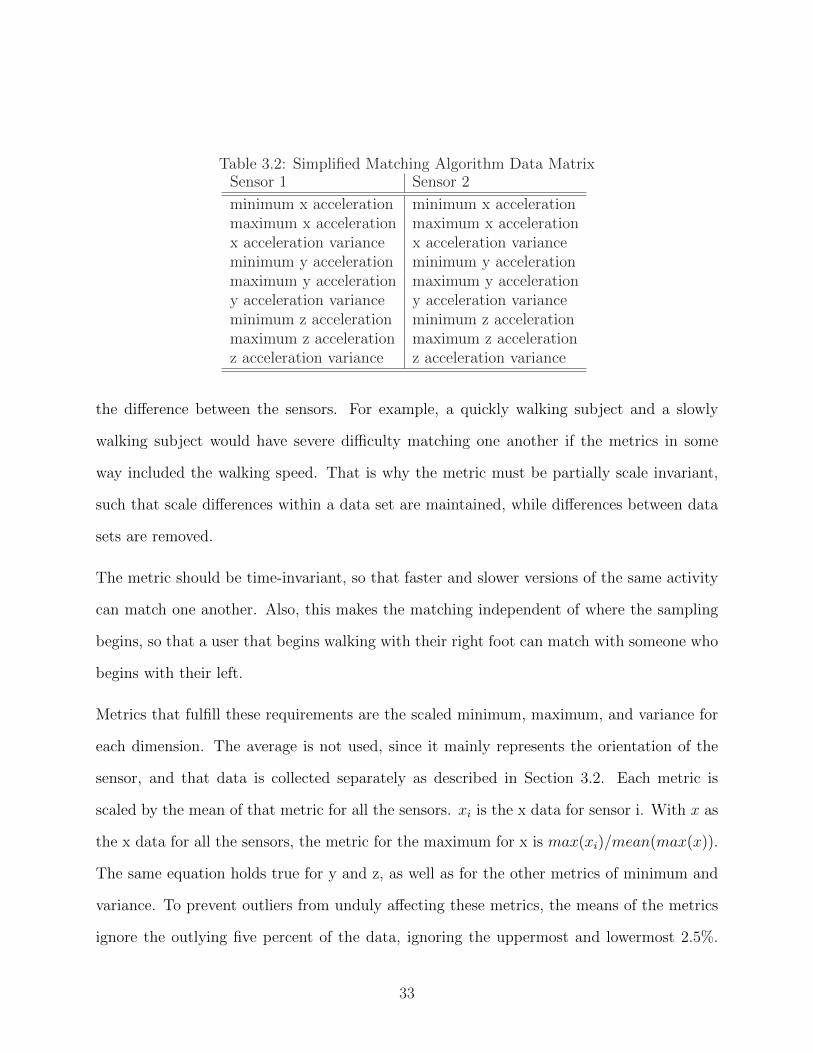
Table 3.2: Simplified Matching Algorithm Data MatrixSensor 1 Sensor 2
minimum x acceleration minimum x accelerationmaximum x acceleration maximum x accelerationx acceleration variance x acceleration varianceminimum y acceleration minimum y accelerationmaximum y acceleration maximum y accelerationy acceleration variance y acceleration varianceminimum z acceleration minimum z accelerationmaximum z acceleration maximum z accelerationz acceleration variance z acceleration variance
the difference between the sensors. For example, a quickly walking subject and a slowly
walking subject would have severe difficulty matching one another if the metrics in some
way included the walking speed. That is why the metric must be partially scale invariant,
such that scale differences within a data set are maintained, while differences between data
sets are removed.
The metric should be time-invariant, so that faster and slower versions of the same activity
can match one another. Also, this makes the matching independent of where the sampling
begins, so that a user that begins walking with their right foot can match with someone who
begins with their left.
Metrics that fulfill these requirements are the scaled minimum, maximum, and variance for
each dimension. The average is not used, since it mainly represents the orientation of the
sensor, and that data is collected separately as described in Section 3.2. Each metric is
scaled by the mean of that metric for all the sensors. xi is the x data for sensor i. With x as
the x data for all the sensors, the metric for the maximum for x is max(xi)/mean(max(x)).
The same equation holds true for y and z, as well as for the other metrics of minimum and
variance. To prevent outliers from unduly affecting these metrics, the means of the metrics
ignore the outlying five percent of the data, ignoring the uppermost and lowermost 2.5%.
33

The maximum metric also ignores the top 1% of the data while the minimum ignores the
bottom 1% of the data. Again, this helps to negate the affect of outliers on these metrics.
The created data matrix uses the selected value of k when performing the SVD. In this case
Ak is a m × n matrix with m as the features for each sensor and n as the sensors for each
training set. The size of Uk is m × k, Sk is k × k, and V Tk is k × n as seen in Equation
3.3. This equation also shows that k is the only free variable which is free to be adjusted
according to the method which was discussed in Section 3.3.3, while m and n are constants
set by the metrics and the number of sensors.
Ak = Uk ∗ Sk ∗ V Tk (3.3)
Training vectors are created by taking the original sensor column vectors, Qt, from m-
dimensional space to k-dimensional space. Equation 3.4 shows that to get the resulting
training vector TVk, the transpose of the column vector is multiplied by the row space in kth
space (Uk) and the inverse of Sk. Each training set creates a training vector for every sensor.
TVk = Qt ∗ Uk ∗ inv(Sk) (3.4)
After all the training vectors are created, the query vectors need to be created. Equation
3.5 shows that this is done in the same manner. A query column Qt is generated for each
sensor in the query set and each column is treated in the same manner as the training data
to get the query vectors.
QVk = Qt ∗ Uk ∗ inv(Sk) (3.5)
34

Now that both the Orientation and SVD algorithms have been shown, the data must be
combined such that the correct sensor configuration is found. This is done through using
a matching algorithm that works on the vectors created from the SVD algorithm and the
orientations found from the Orientation algorithm. The next section discusses this method
in detail.
3.4 Matching Algorithm And Optimization
3.4.1 Training Selection and Culling
The training sets are selected such that each of the sensors has the appropriate orientation.
Mistraining these orientations can have severe consequences on the accuracy of the algorithm.
However, these same problems do not occur when an inappropriate orientation is used for
the query, since the algorithm can correct for small differences and will throw out the data
only if it is severely incorrect.
Determining which training sets are viable requires that these sets meet certain criteria. The
orientation of the sensors must be accurate, and the sensor constellation must be the default
configuration. The subject should also be within the appropriate size constraints. For the
jumpsuit, no user smaller then five foot seven inches is permissible for training. The upper
bound is enforced by the limits of the jumpsuit2.
Other factors may also be important when selecting a training set. These factors will be
tested in Section 4.6.
2Any user that does not fit in the jumpsuit is considered too large.
35

Multiple Training Sets
Multiple training sets must be used in order to prevent certain problems from occurring. Al-
though the training sets are from users performing similar activities, there can be significant
differences between them. When matching, some queries may match well with one of these
training vectors and poorly with the others. The performance of the matching algorithm is
thereby reduced, due to one of the ways that the matching algorithm reduces the complexity
of the problem.
Therefore, multiple training sets are used to create the SVD. When the training vectors are
created, they are averaged into a single master training vector. This is the vector which will
be compared with the query vectors for matching purposes. To determine the number of
training sets which are necessary, the k-selection algorithm is used3. The number of training
sets necessary to train an activity is based upon the stability of this k value once enough
training sets are added to the SVD. This maximum k value will determine how many sets
are needed.
As an example, choose a number of viable training sets which should be much more then
necessary in the final training set selection. For our example, let us choose ten of the sets.
k is found for these ten training sets; in this case, let us say that k = 7. Now the minimum
number of training sets which has k = 7 is found. In this test, this was found to be three
training sets. For the purposes of redundancy and noise reduction, an additional training set
will be added. Therefore, only four training sets are needed, taken from the pool of viable
training sets. These sets can all be from the same subject or from different subjects.
3As discussed in Section 3.3.3, this algorithm selects k such that 95 percent of the data is within k andthe rest is culled.
36

Training Set Selection
There are two important variables when dealing with selection criteria. The first is threshold
selection. This number will influence the false positive rate. The second is training set
selection, the proper selection will improve the overall accuracy of the results.
The way the algorithm is designed, the results are given a confidence number which can vary
from −(n+ 1) to 1, with 1 being the highest confidence and n being the number of sensors.
A sensor configuration is associated with this confidence value. The purpose of the threshold
is to only permit results above a certain confidence value so that a specified accuracy can be
obtained. For example, setting the threshold to 0.99 will guarantee that any results obtained
are correct. However, almost no query will have this high of a confidence value, so there
will be minimal results. This means that the higher the threshold, the higher the number
of false negatives. However, as the threshold drops, the possibility of accepting a result that
is incorrect increases, thereby increasing the number of false positives. Depending on the
requirements of the application, different accuracies will be needed. An ideal solution will
have all of the correct results above the threshold and all of the incorrect answers below the
threshold. However, the data from actual users does not permit an ideal solution and so
techniques to minimize errors must be used.
One reason that lower accuracies may be permissible is if additional tests are done on the
data. If a sensor constellation is repeated as the result for multiple tests, then the probability
that this is the correct result increases. This voting mechanism can be used to increase the
accuracy when the threshold does not guarantee the correct result. This will also allow for
more trials to be above the threshold so that some data can be obtained. If the threshold is
too high, it is possible for none of the trials to have a result.
The data is placed in a table where each row is a trial and each column represents a threshold
37

Table 3.3: Example Threshold Accuracy Table
Threshold0.55 0.75 0.90
Trial 1 1 1 0Trial 2 -1 0 0Trial 3 1 0 0
Table 3.4: Example Threshold Accuracy Percentage
Threshold0.55 0.75 0.90
Accuracy 66% 100% N/APercent Known 100% 33% 0%
value. If the data is correct and above the threshold, then a 1 is used. If the data is incorrect
and above the threshold, -1 is used. Otherwise, the data is below the threshold and a 0 is in
that position. An example can be seen in Table 3.3
The accuracy of a particular threshold can then be obtained via Equation 3.6.
CS ∗ 1002 ∗N + 50 = PA (3.6)
Where CS is the Column Sum, N is the number of known (non-zero) results. The result
PA is an answer from 0 to 100, which is the accuracy as a percentage. The percent of the
data for which we have a result, KP , can be produced using Equation 3.7, with TS as the
total number of rows.
N
TS= KP (3.7)
Table 3.3 produces the accuracy table, Table 3.4. If we were using this data to select a
threshold for further tests, we can see what each value would give. If the threshold was set
38

to 0.90, then we can see that no answers would reach this threshold and so despite its high
accuracy, it would not be useful. If 0.75 is set as the threshold, we get perfect accuracy but
we do not have answers for most of the data set. If 0.55 is set as the threshold, we have
answers for all of the queries and a majority of these answers are correct.
Figure 3.7 shows the percent accuracy of actual data taken from the lower body of the
jumpsuit. The upper red bars represent the percent accuracy for four different training sets
while the lower blue bars represent the known percentage for those self-same sets. The shape
of the markers and the type of line show which percent accuracy is associated with which
known percentage.
For this example, the training sets were not selected with any particular design. This is
solely a representative sample of the type of actual data obtained.
Figure 3.7: Preliminary Results
From this graph we can see that as the threshold increases, so does the accuracy, but less
and less of the data is known. This trade-off of accuracy versus the number of results known
39

is key and shows the importance of properly choosing the threshold for the application.
Differences between the training sets shows that training set selection can also have an
important contribution to the performance of the algorithm. Tests on this interplay can be
seen in Section 4.6.
Culling
The matching algorithm culls the constellations that are below some threshold, tmi. This is a
different threshold then the final accuracy threshold, T . tmi is chosen such that when the full
accuracy is generated, tmi will have reduced this value below T . For example, assume that
T is 0.9 and that there are 3 sensors (n = 3). The value of each match can never be higher
then 1. Therefore, tmi must be at least 0.68, since any lower value will force T below 0.9.
Remember, the matching uses a least squares fit, so 1−((1− .68)2+(1−1)2+(1−1)2) = 0.9.
This is the minimum value for tmi. In practice, min(tmi) ≤ tmi ≤ T . tmi therefore sets the
minimum best match for any specific sensor, while T sets the minimum best match for the
sensor constellation.
When using multiple testing sets, the matching algorithm checks to make certain that at
least one of the sets has a sensor match above tmi. With more sets, this likelihood increases
and therefore reduces the number of sensor constellations that are culled.
3.4.2 Matching Algorithm
For the basic case with fully swappable sensors, and assuming that the number of connector
points is equal to the number of sensors, there exists n! different arrangements of the sensors.
Using a brute force method of trying each of these possibilities against some metric of
accuracy is neither a reasonable nor a scalable solution. Therefore, some method to reduce
40

Table 3.5: Threshold Example
Slot1 2 3 4
Sensors
1 0.95 0.85 0.40 0.402 0.90 0.95 0.50 0.803 0.70 0.60 0.95 0.904 0.60 0.80 0.80 0.95
O(n!) must be generated.
In the current algorithm for determining the position of the sensors, a matrix of values
containing the accuracy of each sensor in every position is first generated. This matrix is
q × r, where q is the number of slots the sensors can be and r is the number of sensors. For
our purposes q = r, so the size of the matrix is r2. This matrix is used as the basis for the
permutation algorithm, which tests all the possibilities to find the one with the best total
fit. The values in the matrix are ≤ 1, with 1 being a perfect fit. Equation 3.8 shows that the
total fit is calculated using a modified least squares equation on the current configuration
values CV ; the closer this number is to 1, the better the fit.
TotalF it = 1−∑(1− CV )2 (3.8)
This best total fit must be above a threshold for the answer to be considered good. As
changing the acceptable threshold also limits the number of answers to queries, variable
thresholds are used so that the behavior can be tailored to the desired application. For the
following examples, however, we use a threshold of 0.9 to clarify how the algorithm works.
As an example, let us use the simple four-sensor suite shown in Table 3.5. As the algorithm
progresses, it will go through the possible permutations. In this example, the correct answer
will be [1 2 3 4], i.e. sensor 1 in slot 1, sensor 2 in slot 2, etc. The brute force method tests
41

every possible ordering. Let us say we are testing the ordering [3 4 2 1]. To check the total
fit, we will use the matrix and find the value for sensor 3 in slot 1, sensor 4 in slot 2, etc.
These are the indices of the matrix and yield the following values [0.7 0.8 0.5 0.4]. Using
Equation 3.8 we get a solution of 0.26. If this were to be the best solution we could obtain,
it would not pass our 0.9 threshold and no configuration would be found. Using the culling
algorithm discussed in Section 3.4.1, this permutation would have been rejected as soon as
the first value of sensor 3 in slot 1 was selected, thereby removing the entire permutation
branch of [3 · · ·]. Now, we can try [2 1 4 3] which yields [0.9 0.85 0.8 0.9] and a total fit value
of 0.9175. This solution would pass our threshold and would be considered a reasonable
solution if no better one is found.
The culling algorithm presented here uses a threshold. Since the total fit must be above
this threshold, data points that are too low will remove that solution from contention. Any
configuration which has a sensor in a location where its match does not reach this threshold
is removed. Since this data can be known before generating the entire configuration, the
entire branch structure below this data point is also removed.
42

Chapter 4
Results
In this chapter, simulation and real data has been used to run the algorithm and the results
from this process are presented. Many of the differences and assumptions are checked to
confirm the accuracy of this methodology.
First, the experimental setup and procedures are explained. Additionally, some of the under-
lying assumptions are checked to confirm that there are no problems. These include testing
the viability of using the threshold to determine the sensor accuracy, testing the minimum
sample size required for good accuracy, and ways to deal with any false positive results.
A thorough analysis of the properties of good and bad training sets follows. Finally, the
algorithm is tested with respect to the different activities and the upper and lower parts of
the jumpsuit.
43

4.1 Experimental Setup
The jumpsuit was woven with wiring embedded as a part of the weave. The wiring consists
of six lines together in a checkerboard pattern. The six lines have two runs of uninsulated
stainless steel on the outside, and the inside four runs are insulated copper wiring. The
current project only uses the four insulated wires. The I2C bus requires four lines: power,
ground, clock, and data (Vin, GND, SCL, and SDA respectively). Since the fabric is woven
with wires in both the warp and the fill, the wire runs are at right angles. These runs are
aligned so that they go up the length of the body or across it, as shown in Figure 4.1. When
connecting to this wiring, there are four straightforward alignments available. Additional
alignments would be difficult to use, and would either twist the wires or require specialized
connector boards. Twisting the wires is not ideal, due to the method of connecting to them,
namely insulation displacement connectors. Twisting this connection could damage the wire
or cause intermittent electrical disconnects. Using specialized connector boards could have
an orientation at something other then at a right angle, but the problems that occur when
adding too many orientations was discussed in Section 3.2.
Figure 4.1: Closeup of Fabric and Sensor
The connectors that are used are insulation displacement connectors (IDCs), a right angle
44

circuit board, and a female USB connection. The IDCs have sharp edges that cut through
the insulator to connect to the wiring inside. Because the IDCs cut the insulation, removing
these connectors damage the embedded wiring. Since the wiring was woven into the garment
as it was being created, these wires are not easily replaced and so care must be taken that
they are not damaged. This is the main reason why once the connectors are placed on the
garment, they are not removed. These connectors also have a static orientation and so any
board that attaches to them will always have the same orientation. A board that connects
to these points uses a male USB connection and communicates over I2C.
The garment currently has a two-tier architecture. Tier 1 consists of the sensors and the
Atmel Atmega8 microcontroller, which samples the sensors at the desired rate and converts
the data to the appropriate I2C format. These microcontrollers also have the capability to
perform simple summary statistics if the full streaming data is not required. However, in
this work, we do not use this capability.
These Tier 1 boards are set up in multi-master mode [18] to connect with a single more
capable Tier 2 board, consisting of a Gumstix Verdex 400xm-bt combined with a special
connector board. The Gumstix currently runs OpenEmbedded Linux and is where the
processing can be done in real time. This board also has a Bluetooth radio, which allows it
to connect to a PC. The PC can be used for display, since the Gumstix does not have that
capability, or the data can be streamed over an ssh connection for later analysis and storage.
Off-line computation and comparisons can be done in this way.
The data that is produced from the sensors contains the sensor ID, an 8 bit counter, and
the sensor data as shown in Table 4.1. The sensor ID is important, since if there is a
heterogeneous system of sensors, this sensor ID will allow us to know the type of data this
sensor is sending. The count can be used to make certain that large blocks of data are not
getting dropped, which can happen if the transmission frequency is set too high. For more
45

Table 4.1: Data FormatByte Number Data
1 Source ID2 Sample Count3
X Acceleration45
Y Acceleration67
Z Acceleration89
Gyro Data10
information about the I2C format and the data transmission, see [18].
Off-line processing is done on Matlab. The data is stored in a basic matlab text file, with
the data grouped by ID and chronology.
The current structure has eleven Tier 1 boards and one Tier 2 board. Since the full data is
streaming over the I2C bus, there is a limit to the sample rate. Currently, the limit for eleven
sensors is approximately 100 Hz for each sensor. If the system is run any faster, collisions on
the bus occur at such a high frequency that some sensors may never get to transmit. If fewer
sensors are on the same bus, the sample rate can go higher [18]. This can lead to additional
complexity in the hierarchy. If additional sensors are desired without negatively impacting
the sensor frequency, the bus may need to be split so that each one contains a subset of the
full Tier 1. In this case, additional Tier 2 nodes can be added to act as routers.
Another option would be to have the matching algorithm split so that each subnet determines
the locations of its sensors. In this case, only the results would need to be transmitted up
the hierarchy. The Tier 2 boards in this case would need to know which subnet they are
on, or would need to be able to determine it from the data that comes in. To do so, the
different subnets would need to be added as part of the training data. The current system
46

uses a single network, since the data rate is still at a reasonable level.
The sensors used for this work are 3D accelerometers and 1D gyroscopes. The accelerometers
are configured so that they can read accelerations from −4 to +4 g. The gyroscopes, which
are not used in all of the test cases, are designed to work from −500 to +500 ◦/s rotation.
Outside of these ranges, the data will peg at the end and clipping will occur. The sensors
are also linearly digitized to a range of 1024 values, which limits the granularity of the data.
The sensors on the jumpsuit are located in the positions shown in figure 4.2. There are
eleven sensors, placed on the upper arms, forearms, hips, thighs, calves, and the chest.
These positions were chosen so that the accelerations of the limbs can be measured, as
described below.
Other than the chest sensor, each of the sensors is actually on the outside of the limb. The
sensor on the left upper arm is on the outside of the body, not in the front. Having the
sensors in these positions adds a few favorable properties to the sensor network. The user
can sit down, something which should not be done if the sensors are on the back of the user.
The user’s arms and legs can be swung freely, whereas if the sensors were on the inside of
the limbs they could rub against the body or one another. The sensors could be placed on
the front of the jumpsuit, as with the chest sensor. However, the current one-dimensional
gyroscopes would be unable to detect rotation in a useful direction, since they can only
read rotation in the plane of the board. Bending to the side could then be detected, but
the normal swinging motion of the limbs would not be. With the sensors on the outside of
the limbs, the rotation from swinging the arms and legs can be detected. Obviously, there
are some motions which do have a side-to-side rotation, but normal ambulatory motion has
rotation in the direction of travel, which is normally forward1.
1Exceptions include crab walking or carwheels, neither of which are widely practiced as the main travelmethod.
47

Figure 4.2: Sensor Positions on the Jumpsuit
4.2 Experimental Procedure
Subjects who are to wear the jumpsuit are first introduced to the garment and are told about
the project and any risks associated with it. In this case, risks are minimal. After signing
the appropriate IRB form discussing all of this information, the procedure is explained to
them. The users are given a pseudonym, which they will be referred to throughout this work.
Selection of a pseudonym will be discussed at the end of this section.
As a first step, the jumpsuit is shown and the sensors and connections are pointed out.
Once the user is ready, they put on the jumpsuit. Identifying the sensors is much easier
while the jumpsuit is not being worn. Pointing out the sensors before the user puts on the
48

jumpsuit helps to prevent the user from unknowingly sitting on a sensor or hitting a sensor
against anything. The risk of damaging a sensor is slight, but not negligible. Once the user
is wearing the jumpsuit to their satisfaction, they are instructed to put their shoes back on,
so that the walking motion is as normal as possible. The user is then instructed to walk
around the area to get accustomed to wearing the jumpsuit and then the next step of the
process is explained.
At this point, the user is instructed to perform the following static activities of standing
and sitting. They also perform some of the following dynamic activities, including stepping
up and down, walking, walking while passing a ball from hand to hand, walking backwards,
walking with arm swing, and walking while bouncing a basketball. Some of the subjects
performed all of these activities, but as there is much duplication between these different
activities, only a subset of them is necessary. For each activity that the subject performed,
at least three trials are captured and checked for glitches.
For some of the subjects, their activities were performed under three different sensor constel-
lations. As there are forty million different constellations possible when using eleven sensors,
only a tiny subset of the possibilities can be tested. The purpose of these tests is to make
certain that any biasing properties of the individual sensors is appropriately removed by the
algorithm. The first sensor constellation is the default configuration and the second one is a
random placement. The third configuration was carefully selected by choosing a worst-case
placement for the sensors with respect to the default constellation. The worst-case selection
is done by analyzing which sensors are most likely to have similar acceleration profiles and
then switching their positions.
After all of the trials are captured, the user removes the jumpsuit and the process is complete.
49

Naming Conventions
The following naming convention is used for the data files. First, there is the code name of the
subject, for example Alex. These names are taken from the list of hurricane names generated
by the National Hurricane Center [22] and have nothing to do with the actual identity of
the subject. The next item in the file name is the activity the subject is performing, e.g.,
walking, and then the trial number is added. Appended to the trial number is the sensor
configuration of the trial. ’D’ is the default configuration, ’C’ is the chosen configuration,
and ’R’ is the random configuration. For some trials, the ’D’ is left out, as any unmarked
data is in the default configuration. Alex Walking 4D is then the fourth walking trial for
subject ’Alex’, using the default sensor configuration.
4.3 Threshold Testing
One of the lynchpins of this design is that the threshold value can be used as a predictor
for the accuracy of a result. Ideally, all of the correct answers would be above a particular
threshold and all of the incorrect answers would be below that threshold. Unfortunately,
when dealing with real people, ideal circumstances do not occur. However, a higher threshold
value should mean that there is a higher chance of a correct answer than an incorrect answer.
One way to check this assertion is to look at the correlation between the threshold and the
correctness. A Spearman Correlation is used because this is not a linear relationship. In fact,
there are only two answers allowed for correctness- Correct and Incorrect. Any datasets for
which there was no answer (for example, the orientations were incorrect) were not used for
this correlation. One important point for discussing the limitations of this method is that if
the data is all correct or all incorrect, no correlation can be found. This is the reason that
50

an aggregate of all of the subjects was used, since some subjects were perfectly accurate. All
of these correlations are accurate to p < .07 (93%) and most of them are accurate to p < .03
or better.
Figure 4.3 shows the correlation values for three different height categories. Short height is
67 or 68 inches, medium is around 71 inches, and tall is around 75 inches. These heights
are relative to the designed ideal height of the jumpsuit, with medium being normal. A
positive correlation, such as that shown here, means that as the threshold increases, so does
the correctness. A negative correlation would mean that a higher threshold results in a lower
accuracy, and a correlation of 0 would mean that there is no relationship between the value
of the threshold and the accuracy.
Figure 4.3: Spearman Correlation of Threshold and Accuracy versus Height
This confirms the accuracy of the threshold as a metric for determining how good the pre-
diction of the sensor constellation will be.
4.4 Sample Size Testing
One variable which can be adjusted to change the performance of the algorithm is the
length of the sample used as the input to the algorithm. Obviously, the sample should be
51

long enough that the full activity is represented. Figure 4.4 shows how the sample size
impacts the accuracy for walking data. A full walking cycle takes about two seconds, and
that can be seen here. With sample sizes below the two second mark, accuracy is reduced,
while data at or above two seconds in length has approximately the same accuracy. As the
different thresholds of the same data set decrease, they allow for more false positives to occur
independently of the sample size.
Figure 4.4: Walking Data Sample Size Versus Accuracy
Additionally, the samples should be offset from the beginning or end of the activity to remove
any artifacts of pre- or post-activity data. These could include the user slowing to a stop or
the change from standing to walking, neither of which are desired.
4.5 Ameliorating Errors
If an application wants to have answers for most of the queries, then the trade-off is a drop in
accuracy. Once the accuracy is below 100%, some method of dealing with inaccurate results
must be used. While other methods may work, a simple voting mechanism will deal with
52

much of the inaccuracy. The effectiveness of this method can be seen through hypothetical
and actual examples.
One possible implementation may consist of a majority rules voting mechanism for deter-
mining the configuration. For example, three queries with the same subject performing the
same activity vote on what the correct configuration is. If any two of them match, then it
is assumed that is the correct configuration. In order to get a 95% confidence that this vote
is correct, the data should be 78% accurate on each query as seen in the following proof,
assuming independence for simplicity.
Want P(At least 2 are correct) = 0.95
P(At least 2 are correct) = 1 - (P(Exactly 2 Incorrect) + P(Exactly 3 Incorrect))
P(Exactly 2 Incorrect) + P(Exactly 3 Incorrect) = 0.05
(1-p)2p + (1-p)3 = 0.05
Let X = (1-p) and (1-X) = p
X2(1-X) + X3 = 0.05
X2 - X3 + X3 = 0.05
X2 = 0.05
X = 0.2236
p = 0.7764 QED
Similarly, if all three of the votes must agree, then each query needs to be 63% accurate.
The overall accuracy can be improved to 99%, requiring each query to be 79% accurate
with the three-vote agreement method.
Figures 4.5 and 4.6 show the different performances when we enforce a specific accuracy.
The required thresholds and percent known are given. If there is no minimum threshold, -1
is used. A lower threshold means that the data is accurate over a long threshold window.
53

Additionally, a high percent known means that there are results for most queries. Ideally,
the entire query set would be above the necessary accuracy, which would remove the need
for a threshold. However, the threshold serves another purpose by eliminated those trials
where the appropriate activity was not performed properly.
Figure 4.5: 80% Accuracy Required Thresholds for Differing Heights
From Figure 4.5, it can be seen that both the tall and medium height training sets yield an
acceptable accuracy at a threshold of -0.2, with the medium height training sets having an
accuracy of above 80% for any threshold in the -1 to 1 region. The shorter training sets were
less acceptable, with a higher required threshold and with less then 20% of the data known
for most of the cases, whereas at least 50% or more of the data was known for the taller
sets. The following Figure 4.6 is for the 64% accuracy threshold, showing that the shorter
training sets can have a larger appropriate threshold window with more known data if the
requirements are relaxed.
However, from Figure 4.6 it can still be seen that while the medium and tall training sets
would satisfy the required accuracy with a threshold of -0.5, the short set would still require
0.2. Even if that data point is disregarded, the shorter training sets still have less of the
data known at the 64% mark.
54

Figure 4.6: 64% Accuracy Required Thresholds for Differing Heights
From these Figures 4.5 and 4.6, it can be seen that the short training sets do not perform as
well as the taller training sets. One of the problems with the shorter training sets is that the
jumpsuit does not fit these subjects very well. Although the tall training sets perform well,
they are not good representative samples of the whole. Thus, the best performance comes
from the average height training sets. A good subject for a training set will fit the jumpsuit
properly while being of approximately medium height. Additional testing on a per subject
basis helps to explain this data and can be seen in the next section.
4.6 Per Training Set and Per Subject Testing
At this point, the properties of a good or bad training set must be found. A baseline set
of results can also be found against which other training sets can be compared to find the
factors which make a difference when selecting training sets.
Table 4.2 shows the number and training set for the data which will follow.
Using the Tukey test, the accuracy results for each subject were compared based on the
55

Table 4.2: Training Set NumbersSet No. Training Set
1 Alex Pacing 1-Alex Pacing 2-Alex Pacing 3-Alex Pacing 42 Alex Walking 1D-Alex Walking 3D-Alex Walking 5D-Alex Walking 7D3 Cesar Walking 1D-Cesar Walking 2D-Cesar Walking 3D-Cesar Walking 4D4 Cesar Walking 5D-Cesar Walking 6D-Cesar Walking 7D-Cesar Walking 8D5 Dean PacingWBall 1-Dean PacingWBall 2-Dean PacingWBall 3-Dean PacingWBall 46 Dean Pacing 1-Dean Pacing 2-Dean Pacing 3-Dean Pacing 47 Earl PacingWBall 1-Earl PacingWBall 2-Earl PacingWBall 3-Earl PacingWBall 48 Earl Pacing 1-Earl Pacing 2-Earl Pacing 3-Earl Pacing 49 Greg PacingWBall 1-Greg PacingWBall 2-Greg PacingWBall 3-Greg PacingWBall 410 Greg Pacing 1-Greg Pacing 2-Greg Pacing 3-Greg Pacing 4
Table 4.3: Tukey Test By SubjectSubject Different Training Set Number Training Set Name
Subject A 5 DeanSubject C 8 EarlSubject D 3,10 Cesar, GregSubject E None N/ASubject F 5 DeanSubject G None N/ASubject I 5 Dean
training set to determine which training sets behaved well and which ones did not based on
the subject. This test was done with 90% confidence that these training sets are significantly
different. The threshold was set to -0.5. The data can be seen in Table 4.3.
From this data, it can be seen that Training Set 5 behaved much differently than the others.
Analyzing how this training set is different from the other training sets will give a good idea
what type of data is not desirable. An analysis of this training set revealed that the problem
actually was due to user error; during one small section of the set a different activity was
occurring. This shows that incorrectly performed training sets have severe consequences
upon the accuracy of the results.
The problems did seem to occur with some basis in height. The shorter subjects had a
56

problem with the taller subjects or with each other. However, other then the aforementioned
problem with Training Set 5, the medium or taller subjects did not have any problems with
the training sets.
To determine the good training sets, the accuracy data for each subject was weighted equally,
such that despite the different number of queries, each training set was treated the same.
Figure 4.7 shows this accuracy and percent known for each training set. From this figure,
it can be seen that Training Sets 3, 4, and 5 all have a performance problem. These are
associated with the shorter subjects. However, Training Set 6, while also associated with
the shorter subjects, has a much better performance. This means that height, while an
important consideration for accuracy, can be ameliorated. This may be due to a different
way that the jumpsuit was fit or aligned during these trials. One thing that may contribute
to the accuracy problems is the fit of the jumpsuit, which is not a problem for taller subjects.
One way to help to make the jumpsuit fit better on the shorter subjects is to add a belt to
keep the sensors in the same area for the different height users. However, this was tried in
Training Sets 3 and 4 without improving the performance. Therefore, the fit problem does
not have much to do with where the waistline is placed on the user and may instead be due
to the overall fit and sensor placement when dealing with shorter subjects.
Looking at Figure 4.7 and using Table 4.2, the training sets which performed the best
belonged to Subjects Alex and Earl, closely followed by Subject Greg. These subjects all
were a good fit for the jumpsuit.
Figure 4.8 shows Training Set 8’s performance versus each Subject. No Subject Cesar or
Henri exists for this figure because they did not perform the appropriate activities for this
test. The only inaccurate data belonged to Subject Bret, but this was a predominately good
set.
57

1 2 3 4 5 6 7 8 9 100
0.1
0.2
0.3
0.4
0.5
0.6
0.7
0.8
0.9
1
Training Set Average Performance
Training Set Number
Fra
ctio
n
AccuracyKnown
Figure 4.7: Lower Body Training Set Average
Figure 4.8: Lower Body Using Training Set 8
58
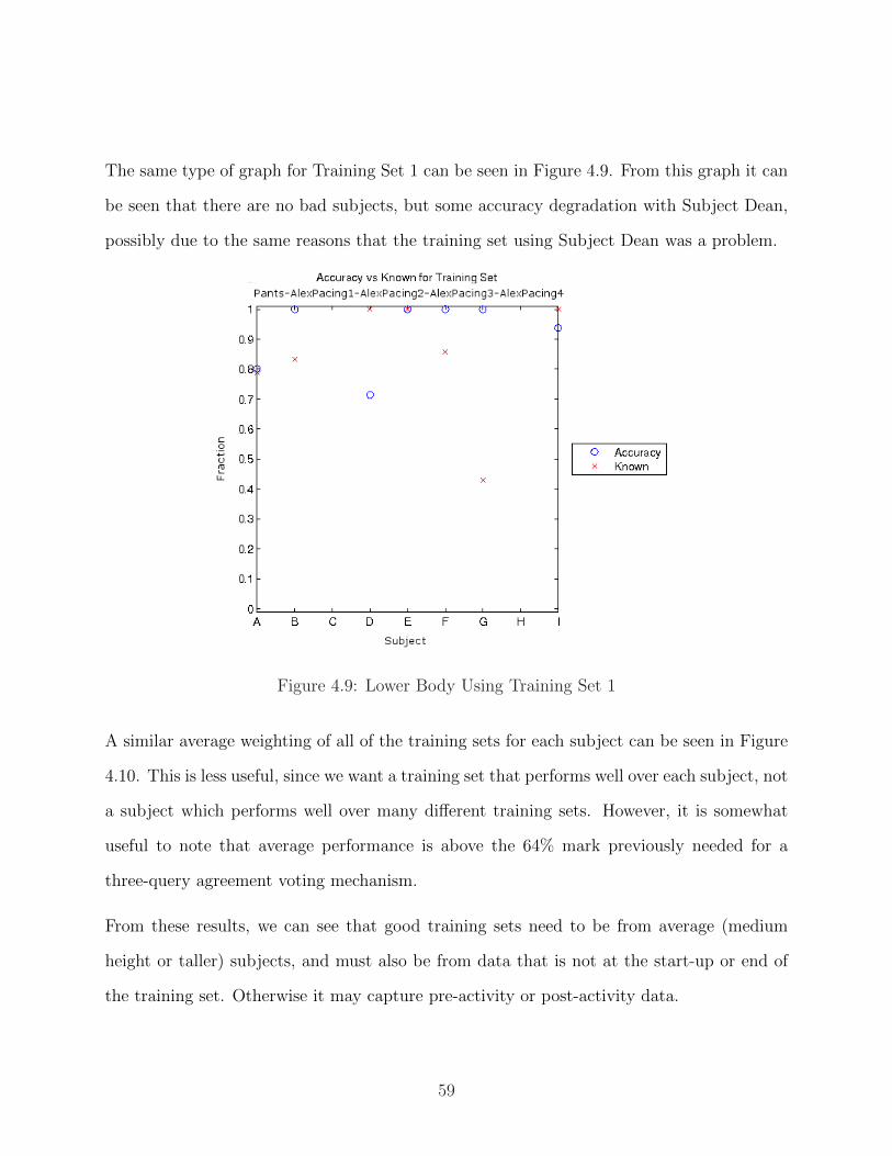
The same type of graph for Training Set 1 can be seen in Figure 4.9. From this graph it can
be seen that there are no bad subjects, but some accuracy degradation with Subject Dean,
possibly due to the same reasons that the training set using Subject Dean was a problem.
Figure 4.9: Lower Body Using Training Set 1
A similar average weighting of all of the training sets for each subject can be seen in Figure
4.10. This is less useful, since we want a training set that performs well over each subject, not
a subject which performs well over many different training sets. However, it is somewhat
useful to note that average performance is above the 64% mark previously needed for a
three-query agreement voting mechanism.
From these results, we can see that good training sets need to be from average (medium
height or taller) subjects, and must also be from data that is not at the start-up or end of
the training set. Otherwise it may capture pre-activity or post-activity data.
59
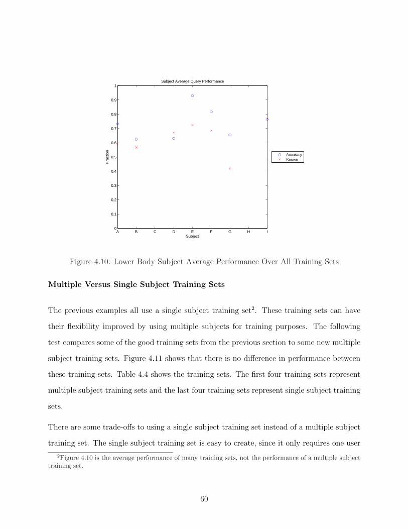
A B C D E F G H I0
0.1
0.2
0.3
0.4
0.5
0.6
0.7
0.8
0.9
1Subject Average Query Performance
Subject
Fra
ctio
n
AccuracyKnown
Figure 4.10: Lower Body Subject Average Performance Over All Training Sets
Multiple Versus Single Subject Training Sets
The previous examples all use a single subject training set2. These training sets can have
their flexibility improved by using multiple subjects for training purposes. The following
test compares some of the good training sets from the previous section to some new multiple
subject training sets. Figure 4.11 shows that there is no difference in performance between
these training sets. Table 4.4 shows the training sets. The first four training sets represent
multiple subject training sets and the last four training sets represent single subject training
sets.
There are some trade-offs to using a single subject training set instead of a multiple subject
training set. The single subject training set is easy to create, since it only requires one user
2Figure 4.10 is the average performance of many training sets, not the performance of a multiple subjecttraining set.
60

Table 4.4: Multiple Versus Single Training Set NumbersSet No. Training Set
1 Alex Pacing 1-Bret Pacing 2-Earl Pacing 2-Felix Pacing 42 Alex Pacing 4-Bret Pacing 2-Dean Pacing 2-Greg Pacing 13 Bret Pacing 3-Dean Pacing 4-Felix Pacing 4-Greg Pacing 34 Bret Pacing 3-Dean Pacing 4-Felix Pacing 4-Greg Pacing 35 Alex Pacing 1-Alex Pacing 2-Alex Pacing 3-Alex Pacing 46 Alex Walking 1D-Alex Walking 3D-Alex Walking 5D-Alex Walking 7D7 Earl PacingWBall 1-Earl PacingWBall 2-Earl PacingWBall 3-Earl PacingWBall 48 Earl Pacing 1-Earl Pacing 2-Earl Pacing 3-Earl Pacing 4
to train on. On the other hand, if there is a problem with the subject, then it propagates
and reduces the accuracy of all of the users. This can even happen if the user is selected
properly but there is a problem with the way the jumpsuit was placed on the subject.
Multiple training sets have a wider variety and so if there is a problem with one of the users,
it will be averaged out by the training sets from the other subjects. In essence, it is easier to
get a good training set from a set containing multiple training sets then from a single training
set, but if a good single subject training set is found, there is no difference in performance.
A representation of the accuracy and errors from the multiple subject training sets can be
seen in the confusion matrix in Table 4.5. This is the sum of the data from four training
sets. From this table it can be seen that there are no orientation errors. It can also be seen
that there are very few errors, of which the majority were errors with the left shin versus
the left thigh.
4.7 Algorithm Testing
Now that the factors that are needed to create a good training set have been found, testing
of the algorithm on a wide range of data to determine its efficacy must be done.
61

1 2 3 4 5 6 7 80
0.1
0.2
0.3
0.4
0.5
0.6
0.7
0.8
0.9
1Training Set Average Performance: Threshold = −0.5
Training Set Number
Fra
ctio
n
AccuracyKnown
Figure 4.11: Multiple (1-4) Versus Single (5-8) Subject Training Sets
Data from CMU’s C3D motion-capture walking data [23] was used to create a simulated
version of the jumpsuit. This data was taken and converted to the same type and restrictions
of the actual data. The restrictions on the data force any accelerations to be within the ±4
g range and any rotations to be within the ±500 ◦/s range. This data is digitized into the
range of 0 - 1024 and then formatted in the same way as the actual data. The data rate for
the simulated jumpsuit is 120 Hz.
Table 4.5: Predicted Versus Actual Sensor PositionPredicted Position
L SHIN R SHIN L THIGH R THIGH L HIP R HIP
Actual Position
L SHIN 140 0 10 0 2 0R SHIN 0 151 0 1 0 0L THIGH 10 0 138 0 4 0R THIGH 0 1 0 150 0 1L HIP 2 0 4 0 146 0R HIP 0 0 0 1 0 151
62

The real jumpsuit data has two different types. In one type, only accelerometers are used.
This set of data ran at 25 Hz. In the second set of data, both accelerometers and gyroscopes
are used. This set of data ran at 100 Hz. In this set of data, the chest sensor was set up
to not use a gyroscope. As the chest sensor has a different orientation then all of the other
sensors, this restriction does not influence the end result, since the orientation portion of the
algorithm has already solved for which sensor is the chest sensor.
The 100 Hz data also used differing sensor configurations, but all training data used the same
default configuration. One of the other sensor configurations was created at random, while
the second one was chosen to cause the worst-case configuration. Throughout all of the tests,
no performance difference was identified between the different sensor configurations. This
shows that the algorithm is sensor-independent. That is, no property of the sensor influences
the algorithm. In the simulation case, there are no differences between the sensors, so the
algorithm will perform the same despite any constellation changes.
The following tests are done on all of the data, restricting all of the sets to the least common
denominator of using solely acceleration data. For this test, the jumpsuit is split into two
distinct sets and processed independently. One reason to split these sections of the jumpsuit
is that the SVD portion of the algorithm leverages the pendulous nature of the human
limbs as previously discussed in Section 2.4.2. To review, when comparing the tangential
acceleration of two pendulums such as an arm and a leg, it becomes very difficult to determine
the difference between certain distances from the joint. For example, the upper arm sensor
and the hip sensor are both close to the joint and can be confused for one another. Also,
an arm movement looks much like a leg movement during walking. Simplistically, both are
swinging pendulums with different lengths where the tangential accelerations are measured
at different points along the pendulum. However, where a normal pendulum would have
considerable difference based on the length, a limb is driven. Therefore, the longer leg could
63

Table 4.6: Simulated Walking Jumpsuit Accuracy Versus ThresholdThreshold Accuracy Percentage Percent Known
0.5 1/1 100% 5.6%0 3/5 60% 28%-0.5 7/14 50% 78%-1 7/16 44% 89%
travel just as fast as the shorter arm making the acceleration profile very similar. Due to
this difficulty and due to the assumption that a normal garment would not be a one-piece,
we have split the sets into upper-body data and lower-body data.
If the upper and lower body are connected to one another, they could connect through a
router or through different ports on the Tier 2 device. Either of these options would allow
the application to determine the difference between the upper and lower body sets. Other
than this assumption that we know if the sensor is on the upper body or the lower body, no
other data is known about the sensors; each sensor on jumpsuit can be connected at any of
the connection sites.
Previous tests were done on a subset of the data, so there may be some differences in
the results from seemingly similar tests. The first test is to confirm that upper and lower
data should remain separate. This is done via a simulation of the full jumpsuit during
normal walking. Table 4.6 shows that it is possible to get a correct answer with a very high
threshold. However, when any reasonable number of answers are desired, the accuracy drops
dramatically, making this full jumpsuit solution far from ideal. This occurs even with the
noiseless simulation data, which should give the best results.
The next series of tests involve the lower-body portion of the jumpsuit, sometimes called
the pants portion. The first test uses the simulation data on the CMU walking subjects.
Table 4.7 shows that the simulated lower-body data yields perfect results and covers most
of the data. This shows that the walking motion works very well for determining the sensor
64

Table 4.7: Simulated Walking Pants Accuracy Versus ThresholdThreshold Accuracy Percentage Percent Known
0.5 3/3 100% 15%0 18/18 100% 90%-0.5 18/18 100% 90%-1 18/18 100% 90%
Table 4.8: Real Walking Pants Accuracy Versus ThresholdThreshold Accuracy Percentage Percent Known
0.5 9/9 100% 11%0 39/43 91% 54%-0.5 48/64 75% 81%-1 49/73 67% 92%
location on the pants of a subject.
This next test uses all of the real jumpsuit data sets which contained a walking motion.
This includes both walking and walking while passing a ball from hand to hand. From Table
4.8 it can be seen that performance is somewhat worse than in simulation. However, high
accuracy can still be obtained while getting results for a majority of the data. Also, note
that if getting perfect accuracy is paramount, it can be obtained, but it requires losing much
of the data.
This next test uses all of the data from the previous tests and adds in subjects that are
dribbling a basketball while walking. From Table 4.9 a decrease in performance can be seen
relative to Table 4.8. This indicates that while there is a walking-type activity occurring
while the user moves forward while dribbling a basketball, it is different enough from a normal
upright walking stance to cause a decrease in accuracy. Noting the variation between these
kinds of activities is important, since it can also be seen that the upper threshold results
maintain their high accuracy, but more of the data is removed from consideration at this
point.
65

Table 4.9: Real Walking Pants Plus Dribbling Accuracy Versus ThresholdThreshold Accuracy Percentage Percent Known
0.5 7/7 100% 6.9%0 20/23 87% 23%-0.5 41/58 70% 56%-1 48/74 65% 72%
Table 4.10: Simulated Walking Shirt Accuracy Versus ThresholdThreshold Accuracy Percentage Percent Known
0.5 8/8 100% 30%0 18/19 95% 70%-0.5 22/24 92% 88%-1 24/26 92% 96%
The following series of tests involve checking the upper-body results, sometimes referred to
as the shirt. First, we must check the simulation results to determine what kind of an upper
bound we can expect. Table 4.10 shows that while walking does not give perfect results in
simulation, it gives very good answers. One difference between the upper and lower body
activities is that the lower body portion of walking is much more standardized between
people. So far as the upper body is concerned, some users hold their arms stiff, some swing
them violently, and others perform somewhere in between. This can cause problems when
trying to match these different subjects.
The following test uses subjects who were told to walk while making certain that their arms
swing naturally. This removes the activities where no motion occurs in the arms while the
user is walking. If there is no arm swing, then obviously the acceleration profiles of the upper
and lower arms are the same. Table 4.11 shows that although some accurate results can be
obtained, the accuracy at the same threshold as a lower body test gives a much lower result.
For example, with this test, a threshold of zero yields 72% accurate, while the worst case for
the pants yielded 87% with many of them above 90%. Therefore, we must try some other
upper-body activities to try and solve this problem.
66

Table 4.11: Real Walking Shirt Accuracy Versus ThresholdThreshold Accuracy Percentage Percent Known
0.5 10/11 91% 37%0 18/25 72% 83%-0.5 20/30 67% 100%-1 20/30 67% 100%
Table 4.12: Lower Body Pacing With Ball Accuracy Versus ThresholdThreshold Accuracy Percentage
0 7/9 77.7%-0.5 10/12 83.3%-1 12/14 85.7%
Table 4.12 show the results when the user is instructed to pass a ball from hand to hand while
walking. Although the results are somewhat higher then those of a purely walking subject,
the distribution of the results is flawed, revealing a deeper problem. The orientation is no
longer effective at separating the left and right forearms because the users held their arms
parallel to the ground, which removed the difference between the sensors. At this point, the
symmetry between the arms in the test causes it to become difficult to determine which one
is which. On the other hand, there were no other errors in this test, so the idea is promising.
A different version of this test which maintains the orientation difference would be a good
upper-body test.
This next test uses the idea of the previous ball tossing and improves upon it. In this test,
the user is instructed to dribble a basketball from hand to hand while walking. Table 4.13
shows that this is a performance increase over the other upper body tests. One way to
see the distribution of the data is shown in Figure 4.12. In this, we can see that as the
threshold increases, there are more and more correct answers and less incorrect ones. Figure
4.12 reveals that the 100% accuracy threshold for this data set is at 0.25. After this point,
incorrect answers begin to occur making it difficult to determine the correctness of a result.
67

Table 4.13: Real Shirt Basketball Accuracy Versus ThresholdThreshold Accuracy Percentage Percent Known
0.5 3/3 100% 13%0 11/13 85% 59%-0.5 16/22 73% 100%-1 16/22 73% 100%
From these results, however, a voting mechanism would be able to determine the upper body
sensor configuration.
Figure 4.12: Histogram of Upper Body Basketball Data
Figure 4.13 summarizes the lower body accuracy results for the simulated walking, real
walking, and real walking and dribbling data. From this figure, it can be seen that the
motion capture data has the highest accuracy. As this data is much less noisy then the
actual sensor data, this is a reasonable result. The other two lower body training sets
perform about the same and show the increase in accuracy as the threshold is raised. If the
99% overall accuracy is required, a three-vote agreement at a threshold between -0.5 and 0
will yield the best results.
Figure 4.14 summarizes the upper body accuracy results for the simulated walking, real
walking, and real dribbling data. Again, the motion capture data has the highest accuracy.
68
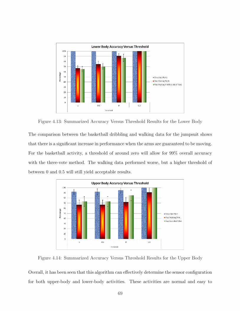
Figure 4.13: Summarized Accuracy Versus Threshold Results for the Lower Body
The comparison between the basketball dribbling and walking data for the jumpsuit shows
that there is a significant increase in performance when the arms are guaranteed to be moving.
For the basketball activity, a threshold of around zero will allow for 99% overall accuracy
with the three-vote method. The walking data performed worse, but a higher threshold of
between 0 and 0.5 will still yield acceptable results.
Figure 4.14: Summarized Accuracy Versus Threshold Results for the Upper Body
Overall, it has been seen that this algorithm can effectively determine the sensor configuration
for both upper-body and lower-body activities. These activities are normal and easy to
69

perform, removing the need for an unusual calibration activity before attempting to use
the jumpsuit. The ability to trade-off the accuracy of the results for additional predicted
configurations can be useful depending on the application. For an application which needs
the correct answer the first time, a high threshold can be used. For applications which can
allow for additional time to perform more queries so that more of the queries are valid, a
voting mechanism can compensate for the lower accuracy.
4.7.1 Voting Testing
For the following voting test, a simple majority with a set window size will not suffice, since
it is not guaranteed to yield an answer. For example, assume a window size of three votes.
Votes are configurations that are above the threshold. Let C be the correct configuration,
and W1, W2, W3 be incorrect configurations. There are more then four total configurations,
but assume only four for simplicity. In the simple majority case with a window size of three,
it is possible to get the votes [W1 C W2]. In this case, no answer would be given. The same
holds true for a window size of five, with the example votes [W1 W1 C C W2]. An example
where a simple majority may not give a good answer can be seen with the votes [W1 W1 C
W2 W3]. In this case, although more votes for W1 occur then for any other configuration, it
does not have an actual majority, which would require three votes. Again, a simple majority
with a window size of seven could also fail to give a good result, with the votes [W1 W1 C
C W2 W2 W3]. Therefore, a simple majority with a set window size will not be used.
Instead, the voting mechanism used in the following tests requires at least three votes for
a specific configuration before making a decision. In essence, the first configuration to get
three votes is considered the winner. Although unnecessary in the following tests due to
the small number of votes, the implementation of the variable windowing system for this
70

mechanism would work according to the following method. First, the window would grow
until a configuration has three votes and thus a result is found. At this point, the window
will contract by removing the oldest votes until no decision can be made. Then, new votes
will be taken to grow the window until a configuration has three votes again. This is exactly
the same idea as a normal sliding window. In a normal three vote sliding window, the first
three votes are taken to yield an answer. Then, the window shrinks by one to give insufficient
data, since there are now only two values while three are required. Then a new vote is taken
to increase the window size back to three so that there is sufficient data to yield an answer
again. The method used for this technique has the same idea, only the window has a variable
size. An example of this mechanism uses the following votes in order: [W1 W1 C W2 C W3
C C C]. A result would be given after the first seven votes [W1 W1 C W2 C W3 C] with the
answer of configuration C. At this point the window will shrink to [W2 C W3 C], removing
the first three votes to get to a point where there is insufficient data. Then, the next vote
will increase the window to [W2 C W3 C C], yielding another result of configuration C.
Then the window will shrink down to [W3 C C] and the next window will be [W3 C C C]
again giving a result of configuration C. Using this mechanism will give a variable sliding
window system that gets periodic results.
For the following voting tests, no simulation data is used, as its data had a short duration
and did not have many repeated subject trials. The voting occurs using subsequent trials
of the same user, so the data is not continuous. As discussed in Section 4.2, if the user
has different sensor configurations, all of the activities are performed for each configuration
before switching to the next one.
Table 4.14 describes the shorthand used in the voting results. The results are either I
- insufficient, C - correct, or W - incorrect. Insufficient data means that there was no
configuration that had at least 3 votes. For the results with insufficient data, a preliminary
71

Table 4.14: Voting Data Legend
I I Insufficient Data, no preliminary solutionI C Insufficient Data, correct preliminary solutionI W Insufficient Data, incorrect preliminary solutionI - Insufficient Data, no votesC x Correct Result, acquired in x votesW x Incorrect Result, acquired in x votes
majority vote is taken. The results of that preliminary vote can also be either I - insufficient,
C - correct, or W - incorrect. A value of ’-’ signifies that no vote occurred. When enough
votes are tallied, the number of votes necessary to get a solution is added after the result.
No sliding window is used, so the full number of votes merely consolidates the result. One
reason that it can take many more votes than the required three to get a solution is that
many different incorrect configurations could all have single votes.
The subject name in each table are followed by an initial representing the sensor config-
uration, with ’D’ as the default configuration, ’C’ as the chosen configuration, and ’R’ as
the random configuration. These configurations were mentioned in Section 4.2. Obviously,
voting was only done using trials which had the same configuration.
The first test is on real lower body data with users performing the walking or walking while
passing a ball from hand to hand activities. Table 4.15 shows that there is only a single
error, which occurs for Subject I below a threshold of -0.5. Other than this problem, all of
the subjects which have enough above-threshold votes yield correct answers. The number of
votes necessary to get a solution decreases as the threshold increases, since fewer bad votes
occur. The best result occurs using a threshold of 0, with correct answers for all of the
subjects that have enough votes. If the threshold is any higher, then all of the answers are
correct, but fewer of the subjects give an answer.
The next test adds users dribbling a basketball while walking to the previous lower body
72

Table 4.15: Real Pants Walking Voting Data
Threshold-1 -0.5 0 0.5
Votes Result Votes Result Votes Result Votes Result
Subject-Config
A - D 13 C 3 10 C 3 4 C 3 2 I CA - C 3 I I 2 I I 0 I - 0 I -B - D 5 C 4 5 C 4 5 C 4 2 I CC - D 8 C 7 5 C 5 3 C 3 0 I -D - D 7 C 3 7 C 3 6 C 3 3 C 3E - D 8 C 3 8 C 3 8 C 3 5 C 3F - D 8 C 3 8 C 3 8 C 3 0 I -G - D 7 C 3 7 C 3 6 C 3 1 I CI - D 7 W 6 6 W 6 0 I - 0 I -I - C 4 I W 3 I I 2 I I 0 I -I - R 3 I C 3 I C 2 I C 0 I -
data, as seen in Table 4.16. All of the results that have enough votes yield correct answers.
To limit the number of votes necessary to obtain a solution, with no loss of accuracy, a
threshold of -0.5 could be used. Raising the threshold much above this reduces the number
of votes and thus the answers obtained. For this test, even a simple majority vote will yield
a correct answer if there are enough votes, regardless of the threshold.
The next test uses the upper body and covers the walking users. Only a subset of the users is
covered in this, so that it can compare with the basketball data, which only was performed by
a subset of the users. Table 4.17 shows that any data receiving enough votes yields a correct
answer. If a simple majority had been used instead of the three vote requirement, then the
default configuration for Subject A would have given an incorrect answer at a threshold of 0.
At lower thresholds with more votes, it can be seen that the results are inconclusive. More
votes at the 0 threshold value should fix this preliminary incorrect result. This sensitivity
to error when dealing with such a small number of votes is why at least three votes for the
same configuration is required before determining the final result. For the tests which give an
answer, at most five votes are needed. The five vote cases for this test occur for the default
73

Table 4.16: Real Pants Walking Plus Dribbling Voting Data
Threshold-1 -0.5 0 0.5
Votes Result Votes Result Votes Result Votes Result
Subject-Config
A - D 12 C 7 9 C 6 3 I I 1 I CA - C 4 I C 3 I I 0 I - 0 I -B - D 6 C 3 5 C 3 0 I - 0 I -C - D 11 C 7 6 C 5 1 I C 0 I -D - D 8 C 4 8 C 4 2 I C 0 I -E - D 7 C 4 7 C 4 6 C 4 2 I CF - D 8 C 5 7 C 4 4 C 3 1 I CG - D 7 C 3 7 C 3 6 C 3 2 I CI - D 6 I I 3 I I 0 I - 0 I -I - C 2 I I 3 I C 1 I C 1 I CI - R 4 I C 0 I - 0 I - 0 I -
Table 4.17: Real Shirt Walking Voting Data
Threshold-1 -0.5 0 0.5
Votes Result Votes Result Votes Result Votes Result
Subject-Config
A - D 6 I I 6 I I 3 I W 0 I -A - C 4 I I 4 I I 2 I I 0 I -C - D 6 C 4 6 C 4 6 C 4 3 C 3I - D 6 C 5 6 C 5 6 C 5 1 I CI - C 4 C 4 4 C 4 4 C 4 3 I CI - R 4 C 3 4 C 3 4 C 3 4 C 3
configuration for Subject I with three votes for the correct configuration and two votes for
an incorrect configuration. After the sixth vote, the number of correct votes increases to
four, cementing its accuracy. Subject A does not give an answer for this test, which ties into
the fact that walking has less upper body motion and can sometimes be difficult to identify.
Therefore, tests on the same subjects using a basketball dribbling activity should have a
performance improvement.
The final test of the upper body data has the users dribbling a basketball while walking as
shown in Table 4.18. For this data, a simple majority vote would also suffice to give correct
74

Table 4.18: Real Shirt Basketball Voting Data
Threshold-1 -0.5 0 0.5
Votes Result Votes Result Votes Result Votes Result
Subject-Config
A - D 1 I C 1 I C 1 I C 0 I -A - C 3 C 3 3 C 3 3 C 3 2 I CA - R 3 I I 3 I I 2 I I 0 I -C - D 5 C 3 5 C 3 3 C 3 1 I CI - D 2 I C 2 I C 1 I C 0 I -I - C 4 C 4 4 C 4 2 I C 0 I -I - R 4 I I 4 I I 1 I C 0 I -
answers for every trial except the random configuration of Subject A. For this set, there is
no bad threshold, since this activity has such a high base accuracy, as was shown in Table
4.13.
Overall, it takes anywhere for three to seven votes to get an answer. Since each vote takes
three seconds, that means that twenty-one seconds of high threshold data should give an
answer. Therefore, using this voting algorithm helps to correct for any errors and will always
give the correct answer with the appropriate threshold settings at the cost of requiring more
time then a single trial test.
75

Chapter 5
Conclusions
This work shows a method by which sensors can be interchanged and replaced on an e-
textile garment and their locations automatically determined. This allows for additional
applications to know where the sensors are located without worrying about hard-coded
sensor position pairs or an out-of-place calibration phase every time something changes on
the garment.
Although the algorithm has difficulties when dealing with symmetrical activities, the appro-
priate sensor orientations can fix this problem entirely. Orientation is a good way to do a
first-pass approximation of the sensor positions, with the algorithm refining the data down
to the exact location.
One problem that was discovered is the difficulty in distinguishing between sensors located
along the arms and legs. If the sensors were restricted to just the end of the arm and the
upper leg, this problem could be ameliorated, but when they are distributed along the entire
length, similarities in the swinging motion cause confusion. Separating the upper and lower
bodies into distinct sets is a reasonable solution to this problem, as most outfits include
76

separate shirts and pants. This would indicate that these networks are at the very least
identifiable subnets of the garment.
Changing the threshold can increase the accuracy of the results, but this increased accuracy
comes at a cost. Less of the queries give results when the threshold is increased. Therefore,
based on the application’s requirements, either high accuracy or a high percentage of results
can be obtained from the queries, but not both. This change to the threshold can also affect
the speed of the application, with additional culling occurring when high thresholds are used.
Using additional trials from the same subject can help to ameliorate the low accuracy when
using lower thresholds. A voting mechanism also helps to confirm that the answer is correct
and thereby increases the overall accuracy. However, this increased accuracy comes at the
cost of additional time required to obtain all of the necessary trials.
5.1 Future Work
Using this work as a baseline, additional locating can be performed on individual sensors.
For example, once the sensor locations are known, the e-textile user may adjust the garment
in such a way, such as rolling up the sleeves, that a sensor is in a different location without
changing its connection point. With the baseline position known, the possible locations
for the moved sensor is limited. One example for this movement would be rolling up the
garment’s sleeves. In this case, sensors on the arm will have a different orientation and, if
rolled up far enough, may change their behavior drastically, with a forearm sensor on the
upper arm, or an ankle sensor at mid-thigh or knee.
This work can also be used as an initial calibration for higher level applications. This
algorithm would be run at first to determine where the sensors are located and then the
77

results can be used in the application. The end application may even collect data during the
calibration step which it will then use once the sensors locations are known, thus saving on
the amount of time a user needs to wear the garment or perform a series of actions.
Additional work can also incorporate more types of sensors. For example, sensitive barome-
ters can detect minuscule differences in air pressure [24]. This could lead to detection of the
difference between the air pressure at different heights on the body. Gyroscopes could also
be added into the algorithm as additional data.
Although preliminary testing revealed that the algorithm could easily distinguish between
static activities and the desired activity, incorporating additional training motions could
yield results for more of the period when the user is wearing the garment. Comparing the
results from different activities could also help to confirm the sensor configuration.
Another area to explore is the real-time implementation of this algorithm and the require-
ments the on-garment processor will need to meet for success. A real-time implementation
could incorporate a rolling vote of the sensor configuration as the garment is worn.
78

Bibliography
[1] C. Einsmann, M. Quirk, B. Muzal, B. Venkatramani, T. Martin, and M. Jones, “Mod-
eling a wearable full-body motion capture system,” in International Symposium on
Wearable Computers, October 2005, pp. 144–151.
[2] V. Jolly, “Activity recognition using singular value decomposition,” Master’s thesis,
Bradley Department of Electrical and Computing Engineering, Virginia Tech, 2006.
[3] “Sensatex Smart Shirt Systems,” http://www.sensatex.com.
[4] “VivoMetrics,” http://www.vivometrics.com.
[5] S. Park and S. Jayaraman, “Smart textiles: Wearable electronic systems,” in MRS
Bulletin, August 2003, pp. 586–591.
[6] E. Post, M. Orth, P. Russo, and N. Gershenfeld, “E-broidery design and fabrication of
textile-based computing,” IBM Systems Journal, vol. 39, no. 3 and 4, 2000.
[7] J. Edmison, M. Jones, Z. Nakad, and T. Martin, “Using piezoelectric materials for
wearable electronic textiles,” in Proceedings of the Sixth International Symposium on
Wearable Computing. ISWC 2002, 2002, pp. 41–48.
[8] “The georgia tech wearable motherboard: The intelligent garment for the 21st century,”
http://www.smartshirt.gatech.edu, 1998.
79

[9] C. R. Merrit, “Fabric-based activite electrode design and fabrication for health monitor-
ing clothing,” in IEEE transactions on information technology in biomedicine, vol. 13,
no. 2, March 2009, pp. 274–280.
[10] K. Kunze, P. Lukowicz, H. Junker, and G. Troester, “Where am I: Recognizing on-body
positions of wearable sensors,” in In: LOCA’04: International Workshop on Locatio-
nand Context-Awareness. Springer-Verlag, 2005, pp. 264–275.
[11] K. Kunze and P. Lukowicz, “Using acceleration signatures from everyday activities for
on-body device location,” in ISWC ’07: Proceedings of the 2007 11th IEEE International
Symposium on Wearable Computers. Washington, DC, USA: IEEE Computer Society,
2007, pp. 1–2.
[12] J. Edmison, M. Jones, T. Lockhart, and T. Martin, “An e-textile system for motion anal-
ysis,” in International Workshop on New Generation of Wearable Systems for eHealth,
December 2003, pp. 215–223.
[13] J. Edmison, “Electronic textiles for motion analysis,” Master’s thesis, Bradley Depart-
ment of Electrical and Computing Engineering, Virgin ia Tech, 2003.
[14] J. Liu, T. Lockhart, M. Jones, and T. Martin, “Local dynamic stability assessment
of motion impaired elderly using electronic textile pants,” Automation Science and
Engineering, IEEE Transactions on, vol. 5, no. 4, pp. 696–702, Oct. 2008.
[15] C. Einsmann, “A validation of a simulation environment for motion sensing electronic
textiles,” Master’s thesis, Bradley Department of Electrical and Computing Engineer-
ing, Virginia Tech, Feb. 2006.
[16] D. C. Lay, Linear Algebra and its appications, second edition update. Addison-Wesley,
1996.
80

[17] M. W. Berry, S. T. Dumais, and G. W. O’Brien, “Using linear algebra for intelligent
information retrieval,” in SIAM Review, 1995, pp. 573–595.
[18] J. Chong, “Activity recognition processing in a self-contained wearable system,” Mas-
ter’s thesis, Bradley Department of Electrical and Computing Engineering, Virginia
Tech, 2008.
[19] M. Rothmaier, M. P. Luong, and F. Clemens, “Textile pressure sensor made of flexible
plastic optical fibers,” Sensors, vol. 8, no. 7, pp. 4318–4329, 2008. [Online]. Available:
http://www.mdpi.com/1424-8220/8/7/4318
[20] Phillips Semiconductors, “The i2c-bus specification,”
http://www.nxp.com/acrobat download/literature/9398/39340011.pdf, Sept 2004.
[21] Dan Schmidt, “Kung FuMonkey Stance,” http://www.expertvillage.com/video/113110 kung-
fu-monkey-stance.htm, 2009.
[22] National Weather Service, “Worldwide Tropical Cyclone Names,”
http://www.nhc.noaa.gov/aboutnames.shtml, Nov 2008.
[23] CMU Graphics Laboratory, “CMU Graphics Lab Motion Capture Database,” 2003.
[Online]. Available: http://mocap.cs.cmu.edu/search.html
[24] Climatronics Corporation, “High Accuracy Barometer,” 2009. [Online]. Available:
http://www.climatronics.com/pdf pn/Atmospheric Pressure/102347.pdf
81