"automatic variational inference in stan" nips2015_yomi2016-01-20

Automatic Variational Inference in Stan

1

2016-01-20 @NIPS 2015_yomi

Yuta Kashino• BakFoo, Inc. CEO

• Zope / Python

• Astro Physics /Observational Cosmology

• Realtime Data Platform for Enterprise

https://vimeo.com/125105210


3

ADVI in Stan

4


Alp KucukelbirColumbia University

[email protected]

Rajesh RanganathPrinceton University

[email protected]

Andrew GelmanColumbia University

[email protected]

David M. BleiColumbia University

[email protected]

Abstract

Variational inference is a scalable technique for approximate Bayesian inference.Deriving variational inference algorithms requires tedious model-specific calcula-tions; this makes it di�cult for non-experts to use. We propose an automatic varia-tional inference algorithm, automatic di�erentiation variational inference (��);we implement it in Stan (code available), a probabilistic programming system. In�� the user provides a Bayesian model and a dataset, nothing else. We makeno conjugacy assumptions and support a broad class of models. The algorithmautomatically determines an appropriate variational family and optimizes the vari-ational objective. We compare �� to �� sampling across hierarchical gen-eralized linear models, nonconjugate matrix factorization, and a mixture model.We train the mixture model on a quarter million images. With �� we can usevariational inference on any model we write in Stan.

1 Introduction

Bayesian inference is a powerful framework for analyzing data. We design a model for data usinglatent variables; we then analyze data by calculating the posterior density of the latent variables. Formachine learning models, calculating the posterior is often di�cult; we resort to approximation.

Variational inference (��) approximates the posterior with a simpler distribution [1, 2]. We searchover a family of simple distributions and find the member closest to the posterior. This turns ap-proximate inference into optimization. �� has had a tremendous impact on machine learning; it istypically faster than Markov chain Monte Carlo (��) sampling (as we show here too) and hasrecently scaled up to massive data [3].

Unfortunately, �� algorithms are di�cult to derive. We must first define the family of approximatingdistributions, and then calculate model-specific quantities relative to that family to solve the varia-tional optimization problem. Both steps require expert knowledge. The resulting algorithm is tied toboth the model and the chosen approximation.

In this paper we develop a method for automating variational inference, automatic di�erentiationvariational inference (��). Given any model from a wide class (specifically, probability modelsdi�erentiable with respect to their latent variables), �� determines an appropriate variational fam-ily and an algorithm for optimizing the corresponding variational objective. We implement �� inStan [4], a flexible probabilistic programming system. Stan describes a high-level language to defineprobabilistic models (e.g., Figure 2) as well as a model compiler, a library of transformations, and ane�cient automatic di�erentiation toolbox. With �� we can now use variational inference on anymodel we write in Stan.1 (See Appendices F to J.)

1�� is available in Stan 2.8. See Appendix C.

1

Objective• Automating Variational Inference (VI)

• ADVI : Automatic Differentiation VI

• give some probability model /w latent variables

• get some data

• inference the latent var.

• Implementation on Stan

5

Objective

6

xn

✓

˛ D 1:5; � D 1

N

data {

i n t N; // number o f o b s e r v a t i o n s

i n t x [N ] ; // d i s c r e t e - valued o b s e r v a t i o n s

}

parameters {

// l a t e n t v a r i a b l e , must be p o s i t i v e

r ea l < lower=0> theta ;

}

model {

// non - conjugate p r i o r f o r l a t e n t v a r i a b l e

theta ~ w e i b u l l ( 1 . 5 , 1) ;

// l i k e l i h o o d

f o r (n in 1 :N)

x [ n ] ~ po i s son ( theta ) ;

}

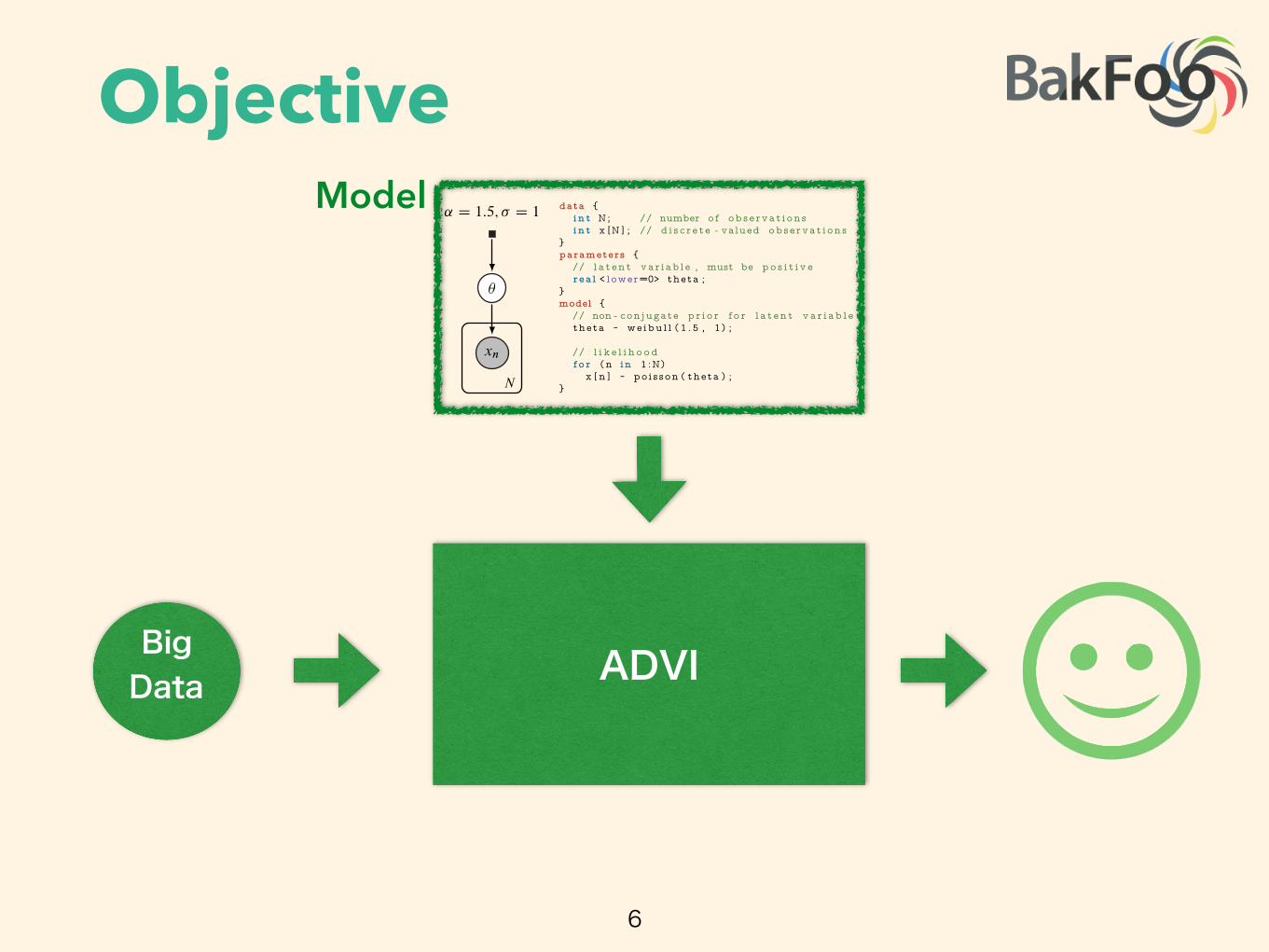
Figure 2: Specifying a simple nonconjugate probability model in Stan.

analysis posits a prior density p.✓/ on the latent variables. Combining the likelihood with the priorgives the joint density p.X; ✓/ D p.X j ✓/ p.✓/.

We focus on approximate inference for di�erentiable probability models. These models have contin-uous latent variables ✓ . They also have a gradient of the log-joint with respect to the latent variablesr✓ log p.X; ✓/. The gradient is valid within the support of the prior supp.p.✓// D

˚

✓ j ✓ 2RK and p.✓/ > 0

✓ RK , where K is the dimension of the latent variable space. This support setis important: it determines the support of the posterior density and plays a key role later in the paper.We make no assumptions about conjugacy, either full or conditional.2

For example, consider a model that contains a Poisson likelihood with unknown rate, p.x j ✓/. Theobserved variable x is discrete; the latent rate ✓ is continuous and positive. Place a Weibull prioron ✓ , defined over the positive real numbers. The resulting joint density describes a nonconjugatedi�erentiable probability model. (See Figure 2.) Its partial derivative @=@✓ p.x; ✓/ is valid within thesupport of the Weibull distribution, supp.p.✓// D RC ⇢ R. Because this model is nonconjugate, theposterior is not a Weibull distribution. This presents a challenge for classical variational inference.In Section 2.3, we will see how �� handles this model.

Many machine learning models are di�erentiable. For example: linear and logistic regression, matrixfactorization with continuous or discrete measurements, linear dynamical systems, and Gaussian pro-cesses. Mixture models, hidden Markov models, and topic models have discrete random variables.Marginalizing out these discrete variables renders these models di�erentiable. (We show an examplein Section 3.3.) However, marginalization is not tractable for all models, such as the Ising model,sigmoid belief networks, and (untruncated) Bayesian nonparametric models.

2.2 Variational Inference

Bayesian inference requires the posterior density p.✓ j X/, which describes how the latent variablesvary when conditioned on a set of observations X. Many posterior densities are intractable becausetheir normalization constants lack closed forms. Thus, we seek to approximate the posterior.

Consider an approximating density q.✓ I �/ parameterized by �. We make no assumptions about itsshape or support. We want to find the parameters of q.✓ I �/ to best match the posterior according tosome loss function. Variational inference (��) minimizes the Kullback-Leibler (��) divergence fromthe approximation to the posterior [2],

�

⇤ D arg min�

KL.q.✓ I �/ k p.✓ j X//: (1)

Typically the �� divergence also lacks a closed form. Instead we maximize the evidence lower bound(��), a proxy to the �� divergence,

L.�/ D Eq.✓/

⇥

log p.X; ✓/

⇤

� Eq.✓/

⇥

log q.✓ I �/

⇤

:

The first term is an expectation of the joint density under the approximation, and the second is theentropy of the variational density. Maximizing the �� minimizes the �� divergence [1, 16].

2The posterior of a fully conjugate model is in the same family as the prior; a conditionally conjugate modelhas this property within the complete conditionals of the model [3].

3

ADVIBig Data

Model

Advantage• very fast

• able to handle big data • no hustle • already available on stan

7

10

210

3

�900

�600

�300

0

Seconds

Aver

age

Log

Pred

ictiv

e

ADVINUTS [5]

(a) Subset of 1000 images

10

210

310

4

�800

�400

0

400

Seconds

Aver

age

Log

Pred

ictiv

e

B=50B=100B=500B=1000

(b) Full dataset of 250 000 images

Figure 1: Held-out predictive accuracy results | Gaussian mixture model (��) of the image��image histogram dataset. (a) �� outperforms the no-U-turn sampler (��), the default samplingmethod in Stan [5]. (b) �� scales to large datasets by subsampling minibatches of size B from thedataset at each iteration [3]. We present more details in Section 3.3 and Appendix J.

Figure 1 illustrates the advantages of our method. Consider a nonconjugate Gaussian mixture modelfor analyzing natural images; this is 40 lines in Stan (Figure 10). Figure 1a illustrates Bayesianinference on 1000 images. The y-axis is held-out likelihood, a measure of model fitness; the x-axis is time on a log scale. �� is orders of magnitude faster than ��, a state-of-the-art ��algorithm (and Stan’s default inference technique) [5]. We also study nonconjugate factorizationmodels and hierarchical generalized linear models in Section 3.

Figure 1b illustrates Bayesian inference on 250 000 images, the size of data we more commonly find inmachine learning. Here we use �� with stochastic variational inference [3], giving an approximateposterior in under two hours. For data like these, �� techniques cannot complete the analysis.

Related work. �� automates variational inference within the Stan probabilistic programmingsystem [4]. This draws on two major themes.

The first is a body of work that aims to generalize ��. Kingma and Welling [6] and Rezende et al.[7] describe a reparameterization of the variational problem that simplifies optimization. Ranganathet al. [8] and Salimans and Knowles [9] propose a black-box technique, one that only requires themodel and the gradient of the approximating family. Titsias and Lázaro-Gredilla [10] leverage thegradient of the joint density for a small class of models. Here we build on and extend these ideas toautomate variational inference; we highlight technical connections as we develop the method.

The second theme is probabilistic programming. Wingate and Weber [11] study �� in general proba-bilistic programs, as supported by languages like Church [12], Venture [13], and Anglican [14]. An-other probabilistic programming system is infer.NET, which implements variational message passing[15], an e�cient algorithm for conditionally conjugate graphical models. Stan supports a more com-prehensive class of nonconjugate models with di�erentiable latent variables; see Section 2.1.

2 Automatic Di�erentiation Variational Inference

Automatic di�erentiation variational inference (��) follows a straightforward recipe. First wetransform the support of the latent variables to the real coordinate space. For example, the logarithmtransforms a positive variable, such as a standard deviation, to the real line. Then we posit a Gaussianvariational distribution to approximate the posterior. This induces a non-Gaussian approximation inthe original variable space. Last we combine automatic di�erentiation with stochastic optimizationto maximize the variational objective. We begin by defining the class of models we support.

2.1 Di�erentiable Probability Models

Consider a dataset X D x1WN with N observations. Each xn is a discrete or continuous random vec-tor. The likelihood p.X j ✓/ relates the observations to a set of latent random variables ✓ . Bayesian

2

Gaussian mixture model (gmm) of the imageCLEF image histogram dataset.

Introduction• VI: difficult to derive

• define the family of approx. distrib.

• solve the variational optimisation prob.

• calculate model-specific quantities

• need expert knowledge

8

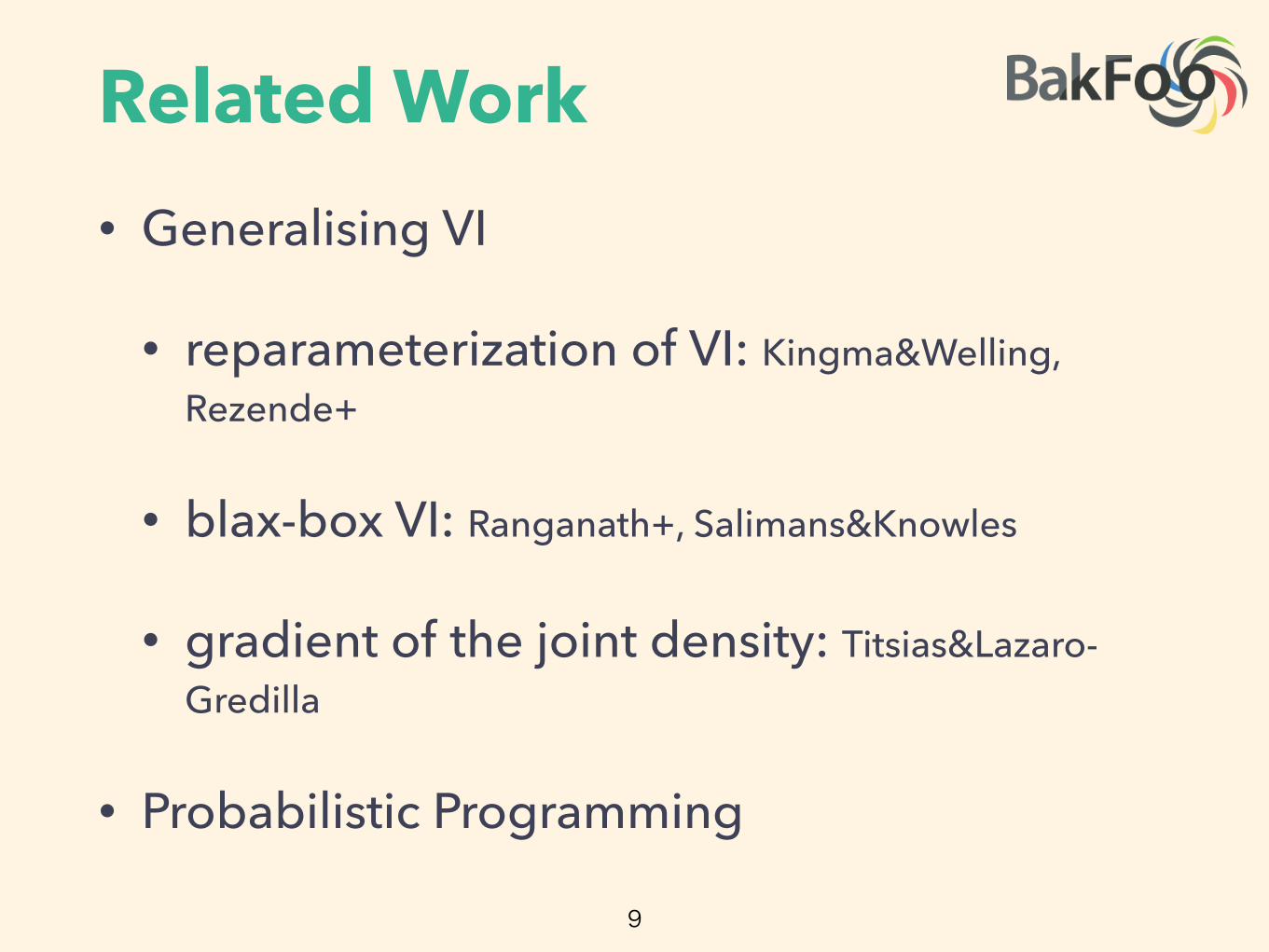
Related Work• Generalising VI

• reparameterization of VI: Kingma&Welling, Rezende+

• blax-box VI: Ranganath+, Salimans&Knowles

• gradient of the joint density: Titsias&Lazaro-Gredilla

• Probabilistic Programming

9

Notations

10

data set X

X

X = x1:N

latent variables ✓

likelifood p(X

X

X|✓)prior density p(✓)

joint density p(X

X

X, ✓) = p(X

X

X|✓)p(✓)log joint gradient r✓log p(XXX, ✓)

support of the prior supp(p(✓)) =

{✓|✓ 2 RKand p(✓) > 0} ✓ RK

Non-Conjugate

11

xn

✓

˛ D 1:5; � D 1

N

data {



}

parameters {



}

model {


theta ~ w e i b u l l ( 1 . 5 , 1) ;


f o r (n in 1 :N)


}




˚

✓ j ✓ 2RK and p.✓/ > 0







�

⇤ D arg min�

KL.

q.✓ I �/ k p.✓ j X/

/: (1)


L.�/ D Eq.✓/

⇥

log p.X; ✓/

⇤

� Eq.✓/

⇥

log q.✓ I �/

⇤

:



3

@@✓p(x, ✓)

is validwithin the support of Weibull diatrib.

supp (p(✓)) = R+ ⇢ R

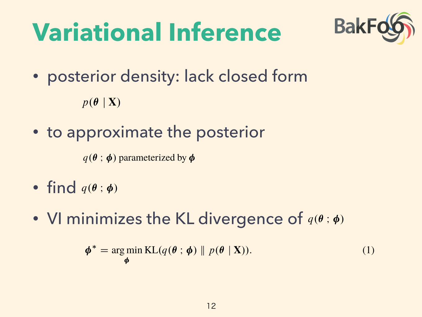
Variational Inference• posterior density: lack closed form

• to approximate the posterior

• find

• VI minimizes the KL divergence of

12

xn

✓

˛ D 1:5; � D 1

N

data {



}

parameters {



}

model {


theta ~ w e i b u l l ( 1 . 5 , 1) ;


f o r (n in 1 :N)


}




˚

✓ j ✓ 2RK and p.✓/ > 0







�

⇤ D arg min�

KL.

q.✓ I �/ k p.✓ j X/

/: (1)


L.�/ D Eq.✓/

⇥

log p.X; ✓/

⇤

� Eq.✓/

⇥

log q.✓ I �/

⇤

:



3

xn

✓

˛ D 1:5; � D 1

N

data {



}

parameters {



}

model {


theta ~ w e i b u l l ( 1 . 5 , 1) ;


f o r (n in 1 :N)


}




˚

✓ j ✓ 2RK and p.✓/ > 0







�

⇤ D arg min�

KL.

q.✓ I �/ k p.✓ j X/

/: (1)


L.�/ D Eq.✓/

⇥

log p.X; ✓/

⇤

� Eq.✓/

⇥

log q.✓ I �/

⇤

:



3

xn

✓

˛ D 1:5; � D 1

N

data {



}

parameters {



}

model {


theta ~ w e i b u l l ( 1 . 5 , 1) ;


f o r (n in 1 :N)


}




˚

✓ j ✓ 2RK and p.✓/ > 0







�

⇤ D arg min�

KL.

q.✓ I �/ k p.✓ j X/

/: (1)


L.�/ D Eq.✓/

⇥

log p.X; ✓/

⇤

� Eq.✓/

⇥

log q.✓ I �/

⇤

:



3

xn

✓

˛ D 1:5; � D 1

N

data {



}

parameters {



}

model {


theta ~ w e i b u l l ( 1 . 5 , 1) ;


f o r (n in 1 :N)


}




˚

✓ j ✓ 2RK and p.✓/ > 0







�

⇤ D arg min�

KL.

q.✓ I �/ k p.✓ j X/

/: (1)


L.�/ D Eq.✓/

⇥

log p.X; ✓/

⇤

� Eq.✓/

⇥

log q.✓ I �/

⇤

:



3

xn

✓

˛ D 1:5; � D 1

N

data {



}

parameters {



}

model {


theta ~ w e i b u l l ( 1 . 5 , 1) ;


f o r (n in 1 :N)


}




˚

✓ j ✓ 2RK and p.✓/ > 0







�

⇤ D arg min�

KL.

q.✓ I �/ k p.✓ j X/

/: (1)


L.�/ D Eq.✓/

⇥

log p.X; ✓/

⇤

� Eq.✓/

⇥

log q.✓ I �/

⇤

:



3

Variational Inference• KL divergence lacks of closed form

• maximize the evidence lower bound (ELBO)

• VI is difficult to automate • non-conjugate • blab-box, fixed v approx.

13

xn

✓

˛ D 1:5; � D 1

N

data {



}

parameters {



}

model {


theta ~ w e i b u l l ( 1 . 5 , 1) ;


f o r (n in 1 :N)


}




˚

✓ j ✓ 2RK and p.✓/ > 0







�

⇤ D arg min�

KL.

q.✓ I �/ k p.✓ j X/

/: (1)


L.�/ D Eq.✓/

⇥

log p.X; ✓/

⇤

� Eq.✓/

⇥

log q.✓ I �/

⇤

:



3

The minimization problem from Eq. (1) becomes

�

⇤ D arg max�

L.�/ such that supp.q.✓ I �// ✓ supp.p.✓ j X//: (2)

We explicitly specify the support-matching constraint implied in the �� divergence.3 We highlightthis constraint, as we do not specify the form of the variational approximation; thus we must ensurethat q.✓ I �/ stays within the support of the posterior, which is defined by the support of the prior.

Why is �� di�cult to automate? In classical variational inference, we typically design a condition-ally conjugate model. Then the optimal approximating family matches the prior. This satisfies thesupport constraint by definition [16]. When we want to approximate models that are not condition-ally conjugate, we carefully study the model and design custom approximations. These depend onthe model and on the choice of the approximating density.

One way to automate �� is to use black-box variational inference [8, 9]. If we select a density whosesupport matches the posterior, then we can directly maximize the �� using Monte Carlo (��)integration and stochastic optimization. Another strategy is to restrict the class of models and use afixed variational approximation [10]. For instance, we may use a Gaussian density for inference inunrestrained di�erentiable probability models, i.e. where supp.p.✓// D RK .

We adopt a transformation-based approach. First we automatically transform the support of the latentvariables in our model to the real coordinate space. Then we posit a Gaussian variational density. Thetransformation induces a non-Gaussian approximation in the original variable space and guaranteesthat it stays within the support of the posterior. Here is how it works.

2.3 Automatic Transformation of Constrained Variables

Begin by transforming the support of the latent variables ✓ such that they live in the real coordinatespace RK . Define a one-to-one di�erentiable function T W supp.p.✓// ! RK and identify thetransformed variables as ⇣ D T .✓/. The transformed joint density g.X; ⇣/ is

g.X; ⇣/ D p

�

X; T

�1.⇣/

�

ˇ

ˇ det JT �1.⇣/

ˇ

ˇ

;

where p is the joint density in the original latent variable space, and JT �1 is the Jacobian of theinverse of T . Transformations of continuous probability densities require a Jacobian; it accounts forhow the transformation warps unit volumes [17]. (See Appendix D.)

Consider again our running example. The rate ✓ lives in RC. The logarithm ⇣ D T .✓/ D log.✓/

transforms RC to the real line R. Its Jacobian adjustment is the derivative of the inverse of thelogarithm, j det JT �1.⇣/j D exp.⇣/. The transformed density is

g.x; ⇣/ D Poisson.x j exp.⇣// Weibull.exp.⇣/ I 1:5; 1/ exp.⇣/:

Figures 3a and 3b depict this transformation.

As we describe in the introduction, we implement our algorithm in Stan to enable generic inference.Stan implements a model compiler that automatically handles transformations. It works by applyinga library of transformations and their corresponding Jacobians to the joint model density.4 Thistransforms the joint density of any di�erentiable probability model to the real coordinate space. Nowwe can choose a variational distribution independent from the model.

2.4 Implicit Non-Gaussian Variational Approximation

After the transformation, the latent variables ⇣ have support on RK . We posit a diagonal (mean-field)Gaussian variational approximation

q.⇣ I �/ D N .

⇣ I �; �

/ DK

Y

kD1

N .⇣k I �k ; �k/:

3If supp.q/ › supp.p/ then outside the support of p we have KL.

q k p

/ D Eq Œlog qç � Eq Œlog pç D �1.4Stan provides transformations for upper and lower bounds, simplex and ordered vectors, and structured

matrices such as covariance matrices and Cholesky factors [4].

4

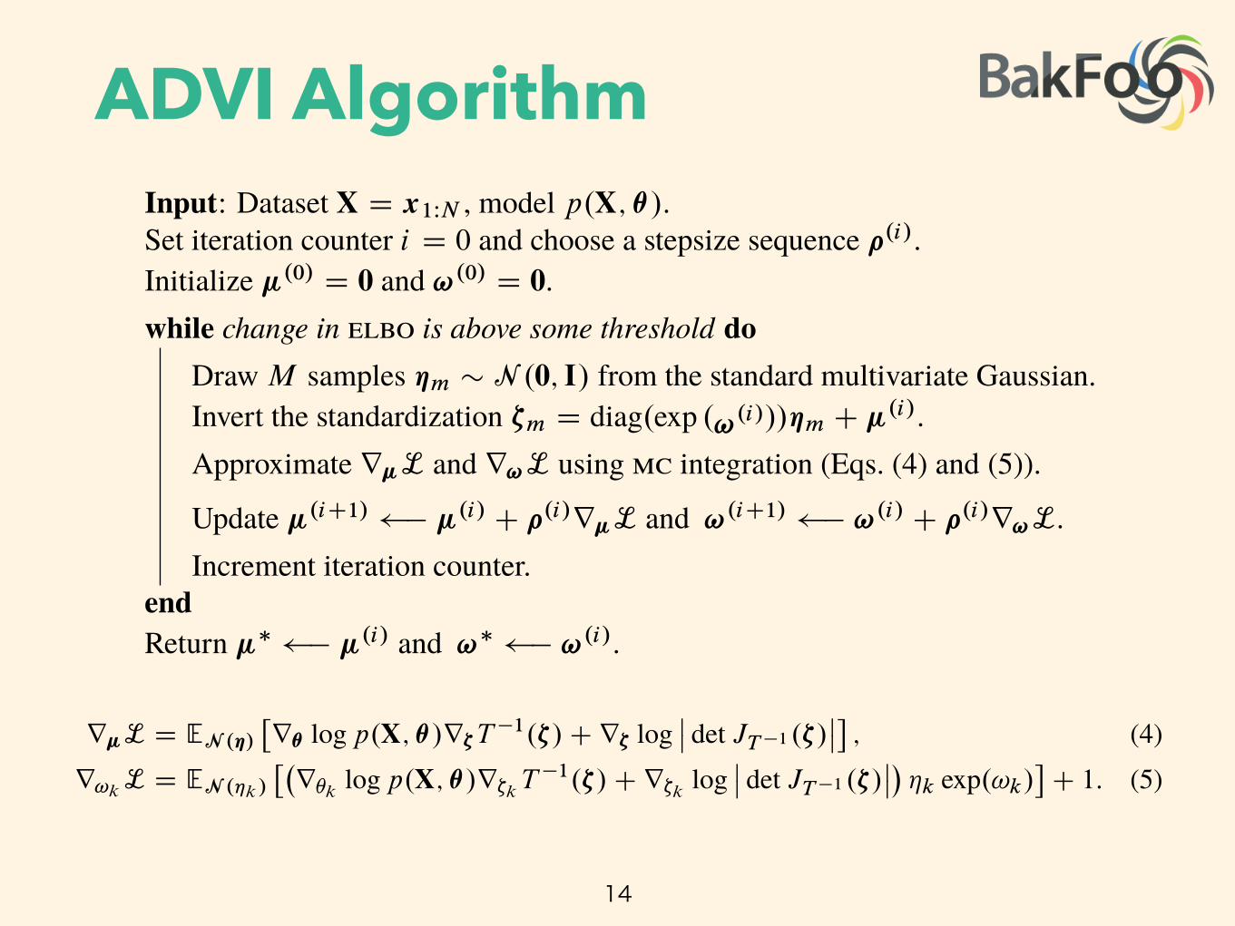
ADVI Algorithm

14

Algorithm 1: Automatic di�erentiation variational inference (��)Input: Dataset X D x1WN , model p.X; ✓/.Set iteration counter i D 0 and choose a stepsize sequence ⇢

.i/.Initialize �

.0/ D 0 and !

.0/ D 0.while change in �� is above some threshold do

Draw M samples ⌘m ⇠ N .0; I/ from the standard multivariate Gaussian.Invert the standardization ⇣m D diag.exp .

!

.i///⌘m C �

.i/.Approximate r�L and r!L using �� integration (Eqs. (4) and (5)).

Update �

.iC1/ � �

.i/ C ⇢

.i/r�L and !

.iC1/ � !

.i/ C ⇢

.i/r!L.Increment iteration counter.

endReturn �

⇤ � �

.i/ and !

⇤ � !

.i/.

encapsulates the variational parameters and gives the fixed density

q.⌘ I 0; I/ D N .

⌘ I 0; I/ D

KY

kD1

N .

⌘k I 0; 1

/:

The standardization transforms the variational problem from Eq. (3) into

�

⇤; !

⇤ D arg max�;!

L.�; !/

D arg max�;!

EN .⌘ I 0;I/

log p

�

X; T

�1.S

�1�;!.⌘//

�

C logˇ

ˇ det JT �1

�

S

�1�;!.⌘/

�

ˇ

ˇ

�

CK

X

kD1

!k ;

where we drop constant terms from the calculation. This expectation is with respect to a standardGaussian and the parameters � and ! are both unconstrained (Figure 3c). We push the gradientinside the expectations and apply the chain rule to get

r�L D EN .⌘/

⇥

r✓ log p.X; ✓/r⇣T

�1.⇣/Cr⇣ log

ˇ

ˇ det JT �1.⇣/

ˇ

ˇ

⇤

; (4)r!k

L D EN .⌘k/

⇥�

r✓klog p.X; ✓/r⇣k

T

�1.⇣/Cr⇣k

logˇ

ˇ det JT �1.⇣/

ˇ

ˇ

�

⌘k exp.!k/

⇤

C 1: (5)

(The derivations are in Appendix B.)

We can now compute the gradients inside the expectation with automatic di�erentiation. The onlything left is the expectation. �� integration provides a simple approximation: draw M samples fromthe standard Gaussian and evaluate the empirical mean of the gradients within the expectation [20].

This gives unbiased noisy gradients of the �� for any di�erentiable probability model. We cannow use these gradients in a stochastic optimization routine to automate variational inference.

2.6 Automatic Variational Inference

Equipped with unbiased noisy gradients of the ��, �� implements stochastic gradient ascent(Algorithm 1). We ensure convergence by choosing a decreasing step-size sequence. In practice, weuse an adaptive sequence [21] with finite memory. (See Appendix E for details.)

�� has complexity O.2NMK/ per iteration, where M is the number of �� samples (typicallybetween 1 and 10). Coordinate ascent �� has complexity O.2NK/ per pass over the dataset. Wescale �� to large datasets using stochastic optimization [3, 10]. The adjustment to Algorithm 1 issimple: sample a minibatch of size B ⌧ N from the dataset and scale the likelihood of the sampledminibatch by N=B [3]. The stochastic extension of �� has per-iteration complexity O.2BMK/.

6


.i/.Initialize �

.0/ D 0 and !



!

.i///⌘m C �


Update �

.iC1/ � �

.i/ C ⇢

.i/r�L and !

.iC1/ � !

.i/ C ⇢


endReturn �

⇤ � �

.i/ and !

⇤ � !

.i/.


q.⌘ I 0; I/ D N .

⌘ I 0; I/ D

KY

kD1

N .

⌘k I 0; 1

/:


�

⇤; !

⇤ D arg max�;!

L.�; !/

D arg max�;!

EN .⌘ I 0;I/

log p

�

X; T

�1.S

�1�;!.⌘//

�

C logˇ

ˇ det JT �1

�

S

�1�;!.⌘/

�

ˇ

ˇ

�

CK

X

kD1

!k ;


r�L D EN .⌘/

⇥


�1.⇣/Cr⇣ log

ˇ

ˇ det JT �1.⇣/

ˇ

ˇ

⇤

; (4)r!k

L D EN .⌘k/

⇥�


T

�1.⇣/Cr⇣k

logˇ

ˇ det JT �1.⇣/

ˇ

ˇ

�

⌘k exp.!k/

⇤

C 1: (5)







6

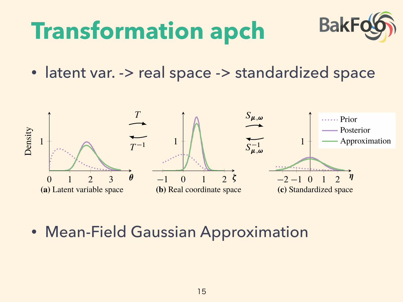
Transformation apch• latent var. -> real space -> standardized space

• Mean-Field Gaussian Approximation

15

0 1 2 3

1

✓

Den

sity

(a) Latent variable space

T

T

�1

�1 0 1 2

1

⇣

(b) Real coordinate space

S�;!

S

�1�;!

�2 �1 0 1 2

1

⌘

PriorPosteriorApproximation

(c) Standardized space

Figure 3: Transformations for ��. The purple line is the posterior. The green line is the approxi-mation. (a) The latent variable space is RC. (a!b) T transforms the latent variable space to R. (b)The variational approximation is a Gaussian. (b!c) S�;! absorbs the parameters of the Gaussian.(c) We maximize the �� in the standardized space, with a fixed standard Gaussian approximation.

The vector � D .�1; � � � ; �K ; �1; � � � ; �K/ contains the mean and standard deviation of each Gaus-sian factor. This defines our variational approximation in the real coordinate space. (Figure 3b.)

The transformation T maps the support of the latent variables to the real coordinate space; its inverseT

�1 maps back to the support of the latent variables. This implicitly defines the variational approx-imation in the original latent variable space as q.T .✓/ I �/

ˇ

ˇ det JT .✓/

ˇ

ˇ

: The transformation ensuresthat the support of this approximation is always bounded by that of the true posterior in the originallatent variable space (Figure 3a). Thus we can freely optimize the �� in the real coordinate space(Figure 3b) without worrying about the support matching constraint.

The �� in the real coordinate space is

L.�; � / D Eq.⇣/

log p

�

X; T

�1.⇣/

�

C logˇ

ˇ det JT �1.⇣/

ˇ

ˇ

�

C K

2

.1C log.2⇡//CK

X

kD1

log �k ;

where we plug in the analytic form of the Gaussian entropy. (The derivation is in Appendix A.)

We choose a diagonal Gaussian for e�ciency. This choice may call to mind the Laplace approxima-tion technique, where a second-order Taylor expansion around the maximum-a-posteriori estimategives a Gaussian approximation to the posterior. However, using a Gaussian variational approxima-tion is not equivalent to the Laplace approximation [18]. The Laplace approximation relies on max-imizing the probability density; it fails with densities that have discontinuities on its boundary. TheGaussian approximation considers probability mass; it does not su�er this degeneracy. Furthermore,our approach is distinct in another way: because of the transformation, the posterior approximationin the original latent variable space (Figure 3a) is non-Gaussian.

2.5 Automatic Di�erentiation for Stochastic Optimization

We now maximize the �� in real coordinate space,

�

⇤; �

⇤ D arg max�;�

L.�; � / such that � � 0: (3)

We use gradient ascent to reach a local maximum of the ��. Unfortunately, we cannot apply auto-matic di�erentiation to the �� in this form. This is because the expectation defines an intractableintegral that depends on � and � ; we cannot directly represent it as a computer program. More-over, the standard deviations in � must remain positive. Thus, we employ one final transformation:elliptical standardization5 [19], shown in Figures 3b and 3c.

First re-parameterize the Gaussian distribution with the log of the standard deviation, ! D log.� /,applied element-wise. The support of ! is now the real coordinate space and � is always positive.Then define the standardization ⌘ D S�;!.⇣/ D diag

�

exp .

!

/

�1�

.⇣ � �/. The standardization

5Also known as a “co-ordinate transformation” [7], an “invertible transformation” [10], and the “re-parameterization trick” [6].

5

Transformation apch• support of latent var > real space

• transformed joint density (Appendix D)

• example:

16


�

⇤ D arg max�








g.X; ⇣/ D p

�

X; T

�1.⇣/

�

ˇ

ˇ det JT �1.⇣/

ˇ

ˇ

;









q.⇣ I �/ D N .

⇣ I �; �

/ DK

Y

kD1

N .⇣k I �k ; �k/:


q k p



4


�

⇤ D arg max�








g.X; ⇣/ D p

�

X; T

�1.⇣/

�

ˇ

ˇ det JT �1.⇣/

ˇ

ˇ

;









q.⇣ I �/ D N .

⇣ I �; �

/ DK

Y

kD1

N .⇣k I �k ; �k/:


q k p



4


�

⇤ D arg max�








g.X; ⇣/ D p

�

X; T

�1.⇣/

�

ˇ

ˇ det JT �1.⇣/

ˇ

ˇ

;









q.⇣ I �/ D N .

⇣ I �; �

/ DK

Y

kD1

N .⇣k I �k ; �k/:


q k p



4

0 1 2 3

1

✓

Den

sity


T

T

�1

�1 0 1 2

1

⇣


S�;!

S

�1�;!

�2 �1 0 1 2

1

⌘







ˇ

ˇ det JT .✓/

ˇ

ˇ



L.�; � / D Eq.⇣/

log p

�

X; T

�1.⇣/

�

C logˇ

ˇ det JT �1.⇣/

ˇ

ˇ

�

C K

2

.1C log.2⇡//CK

X

kD1

log �k ;





�

⇤; �


L.�; � / such that � � 0: (3)



�

exp .

!

/

�1�



5


�

⇤ D arg max�








g.X; ⇣/ D p

�

X; T

�1.⇣/

�

ˇ

ˇ det JT �1.⇣/

ˇ

ˇ

;









q.⇣ I �/ D N .

⇣ I �; �

/ DK

Y

kD1

N .⇣k I �k ; �k/:


q k p



4


�

⇤ D arg max�








g.X; ⇣/ D p

�

X; T

�1.⇣/

�

ˇ

ˇ det JT �1.⇣/

ˇ

ˇ

;









q.⇣ I �/ D N .

⇣ I �; �

/ DK

Y

kD1

N .⇣k I �k ; �k/:


q k p



4

xn

✓

˛ D 1:5; � D 1

N

data {



}

parameters {



}

model {


theta ~ w e i b u l l ( 1 . 5 , 1) ;


f o r (n in 1 :N)


}




˚

✓ j ✓ 2RK and p.✓/ > 0







�

⇤ D arg min�

KL.

q.✓ I �/ k p.✓ j X/

/: (1)


L.�/ D Eq.✓/

⇥

log p.X; ✓/

⇤

� Eq.✓/

⇥

log q.✓ I �/

⇤

:



3


�

⇤ D arg max�








g.X; ⇣/ D p

�

X; T

�1.⇣/

�

ˇ

ˇ det JT �1.⇣/

ˇ

ˇ

;









q.⇣ I �/ D N .

⇣ I �; �

/ DK

Y

kD1

N .⇣k I �k ; �k/:


q k p



4


�

⇤ D arg max�








g.X; ⇣/ D p

�

X; T

�1.⇣/

�

ˇ

ˇ det JT �1.⇣/

ˇ

ˇ

;









q.⇣ I �/ D N .

⇣ I �; �

/ DK

Y

kD1

N .⇣k I �k ; �k/:


q k p



4

MF Gaussian v approx• mean-field Gaussian variational approx

• param vector contain mean/std.deviation

• transformation T ensures the support of approx is always within original latent var.’s

17


�

⇤ D arg max�








g.X; ⇣/ D p

�

X; T

�1.⇣/

�

ˇ

ˇ det JT �1.⇣/

ˇ

ˇ

;









q.⇣ I �/ D N .

⇣ I �; �

/ DK

Y

kD1

N .⇣k I �k ; �k/:


q k p



4

0 1 2 3

1

✓

Den

sity


T

T

�1

�1 0 1 2

1

⇣


S�;!

S

�1�;!

�2 �1 0 1 2

1

⌘







ˇ

ˇ det JT .✓/

ˇ

ˇ



L.�; � / D Eq.⇣/

log p

�

X; T

�1.⇣/

�

C logˇ

ˇ det JT �1.⇣/

ˇ

ˇ

�

C K

2

.1C log.2⇡//CK

X

kD1

log �k ;





�

⇤; �


L.�; � / such that � � 0: (3)



�

exp .

!

/

�1�



5

0 1 2 3

1

✓

Den

sity


T

T

�1

�1 0 1 2

1

⇣


S�;!

S

�1�;!

�2 �1 0 1 2

1

⌘







ˇ

ˇ det JT .✓/

ˇ

ˇ



L.�; � / D Eq.⇣/

log p

�

X; T

�1.⇣/

�

C logˇ

ˇ det JT �1.⇣/

ˇ

ˇ

�

C K

2

.1C log.2⇡//CK

X

kD1

log �k ;





�

⇤; �


L.�; � / such that � � 0: (3)



�

exp .

!

/

�1�



5

MF Gaussian v approx• ELBO of real space (Appendix A)

• MF Gaussian v approx: for efficiency

• original latent var. space is not Gaussian

18

0 1 2 3

1

✓

Den

sity


T

T

�1

�1 0 1 2

1

⇣


S�;!

S

�1�;!

�2 �1 0 1 2

1

⌘







ˇ

ˇ det JT .✓/

ˇ

ˇ



L.�; � / D Eq.⇣/

log p

�

X; T

�1.⇣/

�

C logˇ

ˇ det JT �1.⇣/

ˇ

ˇ

�

C K

2

.1C log.2⇡//CK

X

kD1

log �k ;





�

⇤; �


L.�; � / such that � � 0: (3)



�

exp .

!

/

�1�



5

Gaussian Entropy

0 1 2 3

1

✓

Den

sity


T

T

�1

�1 0 1 2

1

⇣


S�;!

S

�1�;!

�2 �1 0 1 2

1

⌘







ˇ

ˇ det JT .✓/

ˇ

ˇ



L.�; � / D Eq.⇣/

log p

�

X; T

�1.⇣/

�

C logˇ

ˇ det JT �1.⇣/

ˇ

ˇ

�

C K

2

.1C log.2⇡//CK

X

kD1

log �k ;





�

⇤; �


L.�; � / such that � � 0: (3)



�

exp .

!

/

�1�



5

Monte Carlo Integration

Standardization• maximize ELBO in Real space

• intractable integral that depends on μ and σ

• elliptical standardization

• fixed variational density

19

0 1 2 3

1

✓

Den

sity


T

T

�1

�1 0 1 2

1

⇣


S�;!

S

�1�;!

�2 �1 0 1 2

1

⌘







ˇ

ˇ det JT .✓/

ˇ

ˇ



L.�; � / D Eq.⇣/

log p

�

X; T

�1.⇣/

�

C logˇ

ˇ det JT �1.⇣/

ˇ

ˇ

�

C K

2

.1C log.2⇡//CK

X

kD1

log �k ;





�

⇤; �


L.�; � / such that � � 0: (3)



�

exp .

!

/

�1�



5

0 1 2 3

1

✓

Den

sity


T

T

�1

�1 0 1 2

1

⇣


S�;!

S

�1�;!

�2 �1 0 1 2

1

⌘







ˇ

ˇ det JT .✓/

ˇ

ˇ



L.�; � / D Eq.⇣/

log p

�

X; T

�1.⇣/

�

C logˇ

ˇ det JT �1.⇣/

ˇ

ˇ

�

C K

2

.1C log.2⇡//CK

X

kD1

log �k ;





�

⇤; �


L.�; � / such that � � 0: (3)



�

exp .

!

/

�1�



5

2.4 Implicit Non-Gaussian Variational ApproximationAfter the transformation, the latent variables ⇣ have support on RK . We posit a diagonal(mean-field) Gaussian variational approximation

q(⇣ ; �) = N (⇣ ; µ,�

2) =

KY

k=1

N (⇣k ; µk,�2k),

where the vector � = (µ1, · · · , µK ,�

21 , · · · ,�2

K) concatenates the mean and variance of eachGaussian factor. This defines our variational approximation in the real coordinate space.(Figure 3b.)

The transformation T from Equation 3 maps the support of the latent variables tothe real coordinate space. Thus, its inverse T

�1 maps back to the support of the latentvariables. This implicitly defines the variational approximation in the original latent variablespace as N (T

�1(⇣) ; µ,�

2)

�

�

det JT�1(⇣)

�

�

. The transformation ensures that the support of thisapproximation is always bounded by that of the true posterior in the original latent variablespace (Figure 3a). Thus we can freely optimize the elbo in the real coordinate space (Figure3b) without worrying about the support matching constraint.

The elbo in the real coordinate space is

L(µ,�

2) = Eq(⇣)

log p(X, T

�1(⇣)) + log

�

�

det JT�1(⇣)

�

�

�

+

K

2

(1 + log(2⇡)) +

KX

k=1

log �k,

where we plug in the analytic form for the Gaussian entropy. (Derivation in Appendix A.)We choose a diagonal Gaussian for its efficiency and analytic entropy. This choice may

call to mind the Laplace approximation technique, where a second-order Taylor expansionaround the maximum-a-posteriori estimate gives a Gaussian approximation to the poste-rior. However, using a Gaussian variational approximation is not equivalent to the Laplaceapproximation [18]. Our approach is distinct in another way: the posterior approximationin the original latent variable space (Figure 3a) is non-Gaussian, because of the inversetransformation T

�1 and its Jacobian.

2.5 Automatic Differentiation for Stochastic OptimizationWe now seek to maximize the elbo in real coordinate space,

µ

⇤,�

2⇤= arg max

µ,�2

L(µ,�

2) such that �

2 � 0. (4)

We can use gradient ascent to reach a local maximum of the elbo. Unfortunately, we cannotapply automatic differentiation to the elbo in this form. This is because the expectationdefines an intractable integral that depends on µ and �

2; we cannot directly represent itas a computer program. Moreover, the variance vector �

2 must remain positive. Thus, weemploy one final transformation: elliptical standardization6 [19], shown in Figures 3b and3c.

First, re-parameterize the Gaussian distribution with the log of the standard deviation,! = log(�), applied element-wise. The support of ! is now the real coordinate space and � isalways positive. Then, define the standardization ⌘ = Sµ,!(⇣) = diag(exp(!

�1))(⇣�µ). The

standardization encapsulates the variational parameters; in return it gives a fixed variationaldensity

q(⌘ ; 0, I) = N (⌘ ; 0, I) =

KY

k=1

N (⌘k ; 0, 1).

6Also known as a “co-ordinate transformation” [7], an “invertible transformation” [10], and the “re-

parameterization trick” [6].

6

2.4 Implicit Non-Gaussian Variational ApproximationAfter the transformation, the latent variables ⇣ have support on RK . We posit a diagonal(mean-field) Gaussian variational approximation

q(⇣ ; �) = N (⇣ ; µ,�

2) =

KY

k=1

N (⇣k ; µk,�2k),

where the vector � = (µ1, · · · , µK ,�

21 , · · · ,�2

K) concatenates the mean and variance of eachGaussian factor. This defines our variational approximation in the real coordinate space.(Figure 3b.)

The transformation T from Equation 3 maps the support of the latent variables tothe real coordinate space. Thus, its inverse T

�1 maps back to the support of the latentvariables. This implicitly defines the variational approximation in the original latent variablespace as N (T

�1(⇣) ; µ,�

2)

�

�

det JT�1(⇣)

�

�

. The transformation ensures that the support of thisapproximation is always bounded by that of the true posterior in the original latent variablespace (Figure 3a). Thus we can freely optimize the elbo in the real coordinate space (Figure3b) without worrying about the support matching constraint.

The elbo in the real coordinate space is

L(µ,�

2) = Eq(⇣)

log p(X, T

�1(⇣)) + log

�

�

det JT�1(⇣)

�

�

�

+

K

2

(1 + log(2⇡)) +

KX

k=1

log �k,

where we plug in the analytic form for the Gaussian entropy. (Derivation in Appendix A.)We choose a diagonal Gaussian for its efficiency and analytic entropy. This choice may

call to mind the Laplace approximation technique, where a second-order Taylor expansionaround the maximum-a-posteriori estimate gives a Gaussian approximation to the poste-rior. However, using a Gaussian variational approximation is not equivalent to the Laplaceapproximation [18]. Our approach is distinct in another way: the posterior approximationin the original latent variable space (Figure 3a) is non-Gaussian, because of the inversetransformation T

�1 and its Jacobian.

2.5 Automatic Differentiation for Stochastic OptimizationWe now seek to maximize the elbo in real coordinate space,

µ

⇤,�

2⇤= arg max

µ,�2

L(µ,�

2) such that �

2 � 0. (4)

We can use gradient ascent to reach a local maximum of the elbo. Unfortunately, we cannotapply automatic differentiation to the elbo in this form. This is because the expectationdefines an intractable integral that depends on µ and �

2; we cannot directly represent itas a computer program. Moreover, the variance vector �

2 must remain positive. Thus, weemploy one final transformation: elliptical standardization6 [19], shown in Figures 3b and3c.

First, re-parameterize the Gaussian distribution with the log of the standard deviation,! = log(�), applied element-wise. The support of ! is now the real coordinate space and � isalways positive. Then, define the standardization ⌘ = Sµ,!(⇣) = diag(exp(!

�1))(⇣�µ). The

standardization encapsulates the variational parameters; in return it gives a fixed variationaldensity

q(⌘ ; 0, I) = N (⌘ ; 0, I) =

KY

k=1

N (⌘k ; 0, 1).

6Also known as a “co-ordinate transformation” [7], an “invertible transformation” [10], and the “re-

parameterization trick” [6].

6

0 1 2 3

1

✓

Den

sity


T

T

�1

�1 0 1 2

1

⇣


S�;!

S

�1�;!

�2 �1 0 1 2

1

⌘







ˇ

ˇ det JT .✓/

ˇ

ˇ



L.�; � / D Eq.⇣/

log p

�

X; T

�1.⇣/

�

C logˇ

ˇ det JT �1.⇣/

ˇ

ˇ

�

C K

2

.1C log.2⇡//CK

X

kD1

log �k ;





�

⇤; �


L.�; � / such that � � 0: (3)



�

exp .

!

/

�1�



5

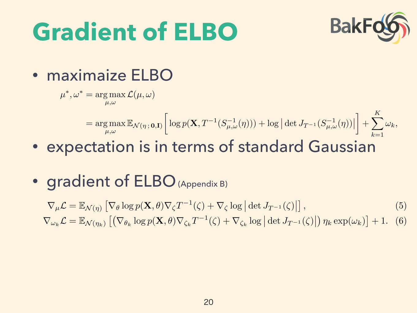
Gradient of ELBO• maximaize ELBO

• expectation is in terms of standard Gaussian

• gradient of ELBO (Appendix B)

20

Algorithm 1: Automatic Differentiation Variational Inference

Input: Dataset X = x1:N , model p(X, ✓).Set iteration counter i = 0 and choose a stepsize sequence ⇢

(i).Initialize µ

(0)= 0 and !

(0)= 0.

while change in elbo is above some threshold doDraw M samples ⌘m ⇠ N (0, I) from the standard multivariate Gaussian.

Invert the standardization ⇣m = diag(exp(!

(i)))⌘m + µ

(i).Approximate rµL and r!L using mc integration (Equations 5 and 6).

Update µ

(i+1) � µ

(i)+ ⇢

(i)rµL and !

(i+1) � !

(i)+ ⇢

(i)r!L.Increment iteration counter.

endReturn µ

⇤ � µ

(i) and !

⇤ � !

(i).

The standardization transforms the variational problem from Equation 4 into

µ

⇤,!

⇤= arg max

µ,!L(µ,!)

= arg max

µ,!EN (⌘ ; 0,I)

log p(X, T

�1(S

�1µ,!(⌘))) + log

�

�

det JT�1(S

�1µ,!(⌘))

�

�

�

+

KX

k=1

!k,

where we drop independent term from the calculation. The expectation is now in terms ofthe standard Gaussian, and both parameters µ and ! are unconstrained. (Figure 3c.) Wepush the gradient inside the expectations and apply the chain rule to get

rµL = EN (⌘)

⇥r✓ log p(X, ✓)r⇣T�1

(⇣) +r⇣ log

�

�

det JT�1(⇣)

�

�

⇤

, (5)r!kL = EN (⌘k)

⇥�r✓k log p(X, ✓)r⇣kT�1

(⇣) +r⇣k log

�

�

det JT�1(⇣)

�

�

�

⌘k exp(!k)⇤

+ 1. (6)

(Derivations in Appendix B.)We can now compute the gradients inside the expectation with automatic differentiation.

This leaves only the expectation. mc integration provides a simple approximation: drawM samples from the standard Gaussian and evaluate the empirical mean of the gradientswithin the expectation [20]. This gives unbiased noisy estimates of gradients of the elbo.

2.6 Scalable Automatic Variational InferenceEquipped with unbiased noisy gradients of the elbo, advi implements stochastic gradientascent. (Algorithm 1.) We ensure convergence by choosing a decreasing step-size schedule.In practice, we use an adaptive schedule [21] with finite memory. (See Appendix E fordetails.)

advi has complexity O(2NMK) per iteration, where M is the number of mc samples(typically between 1 and 10). Coordinate ascent vi has complexity O(2NK) per pass overthe dataset. We scale advi to large datasets using stochastic optimization [3, 10]. Theadjustment to Algorithm 1 is simple: sample a minibatch of size B ⌧ N from the datasetand scale the likelihood of the model by N/B [3]. The stochastic extension of advi has aper-iteration complexity O(2BMK).

3 Empirical StudyWe now study advi across a variety of models. We compare its speed and accuracy to twoMarkov chain Monte Carlo (mcmc) sampling algorithms: Hamiltonian Monte Carlo (hmc)

7

Algorithm 1: Automatic Differentiation Variational Inference

Input: Dataset X = x1:N , model p(X, ✓).Set iteration counter i = 0 and choose a stepsize sequence ⇢

(i).Initialize µ

(0)= 0 and !

(0)= 0.

while change in elbo is above some threshold doDraw M samples ⌘m ⇠ N (0, I) from the standard multivariate Gaussian.

Invert the standardization ⇣m = diag(exp(!

(i)))⌘m + µ

(i).Approximate rµL and r!L using mc integration (Equations 5 and 6).

Update µ

(i+1) � µ

(i)+ ⇢

(i)rµL and !

(i+1) � !

(i)+ ⇢

(i)r!L.Increment iteration counter.

endReturn µ

⇤ � µ

(i) and !

⇤ � !

(i).

The standardization transforms the variational problem from Equation 4 into

µ

⇤,!

⇤= arg max

µ,!L(µ,!)

= arg max

µ,!EN (⌘ ; 0,I)

log p(X, T

�1(S

�1µ,!(⌘))) + log

�

�

det JT�1(S

�1µ,!(⌘))

�

�

�

+

KX

k=1

!k,

where we drop independent term from the calculation. The expectation is now in terms ofthe standard Gaussian, and both parameters µ and ! are unconstrained. (Figure 3c.) Wepush the gradient inside the expectations and apply the chain rule to get

rµL = EN (⌘)

⇥r✓ log p(X, ✓)r⇣T�1

(⇣) +r⇣ log

�

�

det JT�1(⇣)

�

�

⇤

, (5)r!kL = EN (⌘k)

⇥�r✓k log p(X, ✓)r⇣kT�1

(⇣) +r⇣k log

�

�

det JT�1(⇣)

�

�

�

⌘k exp(!k)⇤

+ 1. (6)

(Derivations in Appendix B.)We can now compute the gradients inside the expectation with automatic differentiation.

This leaves only the expectation. mc integration provides a simple approximation: drawM samples from the standard Gaussian and evaluate the empirical mean of the gradientswithin the expectation [20]. This gives unbiased noisy estimates of gradients of the elbo.

2.6 Scalable Automatic Variational InferenceEquipped with unbiased noisy gradients of the elbo, advi implements stochastic gradientascent. (Algorithm 1.) We ensure convergence by choosing a decreasing step-size schedule.In practice, we use an adaptive schedule [21] with finite memory. (See Appendix E fordetails.)

advi has complexity O(2NMK) per iteration, where M is the number of mc samples(typically between 1 and 10). Coordinate ascent vi has complexity O(2NK) per pass overthe dataset. We scale advi to large datasets using stochastic optimization [3, 10]. Theadjustment to Algorithm 1 is simple: sample a minibatch of size B ⌧ N from the datasetand scale the likelihood of the model by N/B [3]. The stochastic extension of advi has aper-iteration complexity O(2BMK).

3 Empirical StudyWe now study advi across a variety of models. We compare its speed and accuracy to twoMarkov chain Monte Carlo (mcmc) sampling algorithms: Hamiltonian Monte Carlo (hmc)

7

ADVI Algorithm

21


.i/.Initialize �

.0/ D 0 and !



!

.i///⌘m C �


Update �

.iC1/ � �

.i/ C ⇢

.i/r�L and !

.iC1/ � !

.i/ C ⇢


endReturn �

⇤ � �

.i/ and !

⇤ � !

.i/.


q.⌘ I 0; I/ D N .

⌘ I 0; I/ D

KY

kD1

N .

⌘k I 0; 1

/:


�

⇤; !

⇤ D arg max�;!

L.�; !/

D arg max�;!

EN .⌘ I 0;I/

log p

�

X; T

�1.S

�1�;!.⌘//

�

C logˇ

ˇ det JT �1

�

S

�1�;!.⌘/

�

ˇ

ˇ

�

CK

X

kD1

!k ;


r�L D EN .⌘/

⇥


�1.⇣/Cr⇣ log

ˇ

ˇ det JT �1.⇣/

ˇ

ˇ

⇤

; (4)r!k

L D EN .⌘k/

⇥�


T

�1.⇣/Cr⇣k

logˇ

ˇ det JT �1.⇣/

ˇ

ˇ

�

⌘k exp.!k/

⇤

C 1: (5)







6


.i/.Initialize �

.0/ D 0 and !



!

.i///⌘m C �


Update �

.iC1/ � �

.i/ C ⇢

.i/r�L and !

.iC1/ � !

.i/ C ⇢


endReturn �

⇤ � �

.i/ and !

⇤ � !

.i/.


q.⌘ I 0; I/ D N .

⌘ I 0; I/ D

KY

kD1

N .

⌘k I 0; 1

/:


�

⇤; !

⇤ D arg max�;!

L.�; !/

D arg max�;!

EN .⌘ I 0;I/

log p

�

X; T

�1.S

�1�;!.⌘//

�

C logˇ

ˇ det JT �1

�

S

�1�;!.⌘/

�

ˇ

ˇ

�

CK

X

kD1

!k ;


r�L D EN .⌘/

⇥


�1.⇣/Cr⇣ log

ˇ

ˇ det JT �1.⇣/

ˇ

ˇ

⇤

; (4)r!k

L D EN .⌘k/

⇥�


T

�1.⇣/Cr⇣k

logˇ

ˇ det JT �1.⇣/

ˇ

ˇ

�

⌘k exp.!k/

⇤

C 1: (5)







6

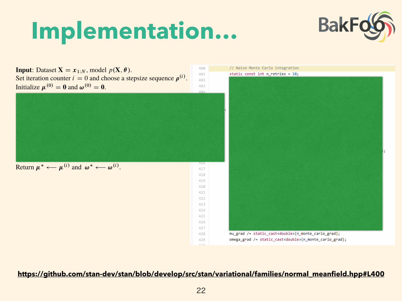
Implementation…

22


.i/.Initialize �

.0/ D 0 and !



!

.i///⌘m C �


Update �

.iC1/ � �

.i/ C ⇢

.i/r�L and !

.iC1/ � !

.i/ C ⇢


endReturn �

⇤ � �

.i/ and !

⇤ � !

.i/.


q.⌘ I 0; I/ D N .

⌘ I 0; I/ D

KY

kD1

N .

⌘k I 0; 1

/:


�

⇤; !

⇤ D arg max�;!

L.�; !/

D arg max�;!

EN .⌘ I 0;I/

log p

�

X; T

�1.S

�1�;!.⌘//

�

C logˇ

ˇ det JT �1

�

S

�1�;!.⌘/

�

ˇ

ˇ

�

CK

X

kD1

!k ;


r�L D EN .⌘/

⇥


�1.⇣/Cr⇣ log

ˇ

ˇ det JT �1.⇣/

ˇ

ˇ

⇤

; (4)r!k

L D EN .⌘k/

⇥�


T

�1.⇣/Cr⇣k

logˇ

ˇ det JT �1.⇣/

ˇ

ˇ

�

⌘k exp.!k/

⇤

C 1: (5)







6

https://github.com/stan-dev/stan/blob/develop/src/stan/variational/families/normal_meanfield.hpp#L400

https://github.com/stan-dev/stan/blob/develop/src/stan/variational/families/normal_meanfield.hpp#L400

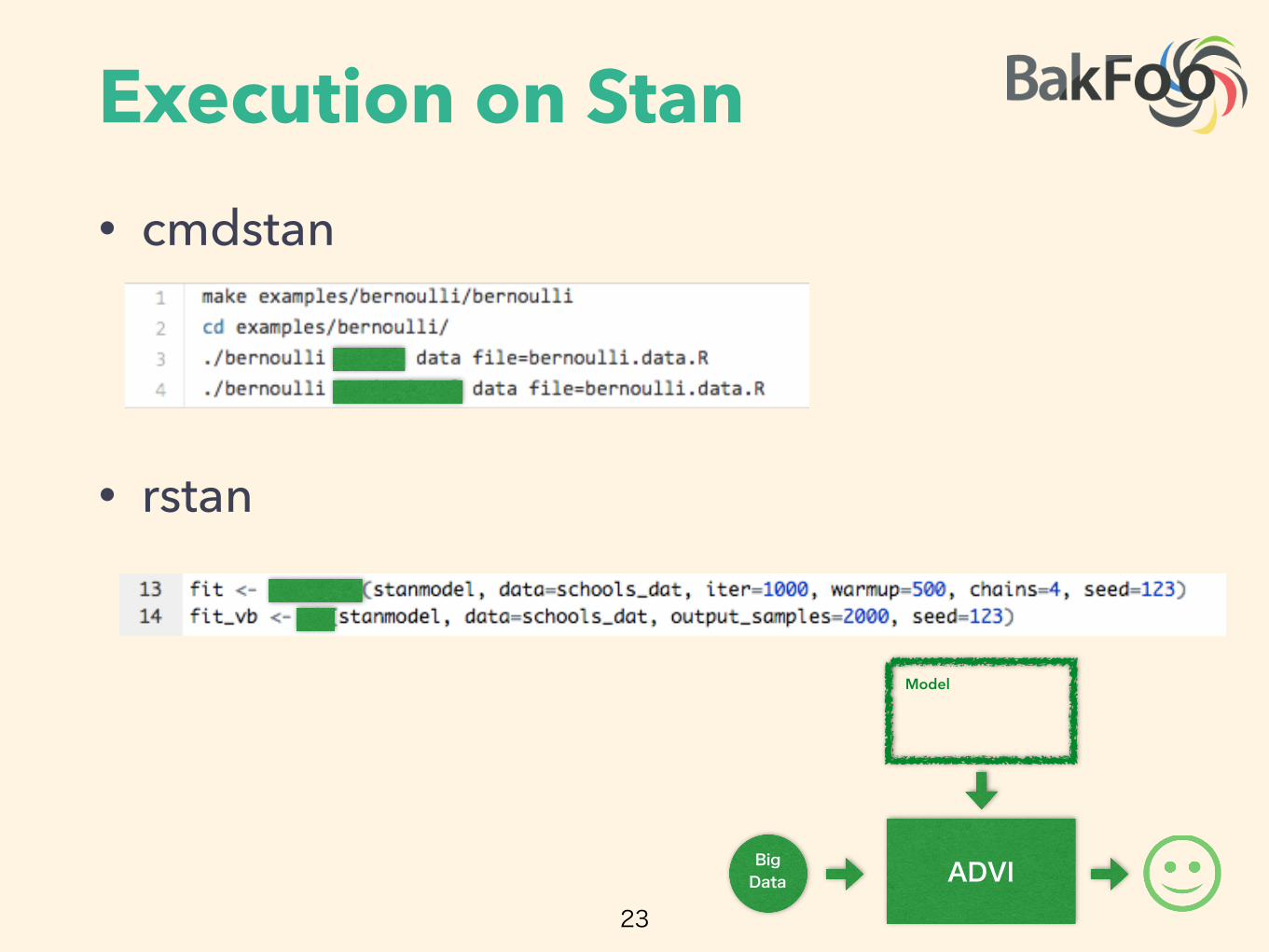
Execution on Stan• cmdstan

• rstan

23

ADVIBig Data

Model

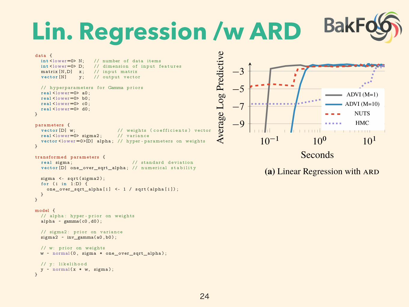
Lin. Regression /w ARD

24

10

�110

010

1

�9

�7

�5

�3

Seconds

Aver

age

Log

Pred

ictiv

e

ADVI (M=1)ADVI (M=10)

NUTSHMC

(a) Linear Regression with ��

10

�110

010

110

2

�1:5

�1:3

�1:1

�0:9

�0:7

Seconds

Aver

age

Log

Pred

ictiv

e


NUTSHMC

(b) Hierarchical Logistic Regression

Figure 4: Hierarchical generalized linear models. Comparison of �� to ��: held-out predic-tive likelihood as a function of wall time.

3 Empirical Study

We now study �� across a variety of models. We compare its speed and accuracy to two Markovchain Monte Carlo (��) sampling algorithms: Hamiltonian Monte Carlo (��) [22] and the no-U-turn sampler (��)6 [5]. We assess �� convergence by tracking the ��. To place �� and�� on a common scale, we report predictive likelihood on held-out data as a function of time. Weapproximate the posterior predictive likelihood using a �� estimate. For ��, we plug in posteriorsamples. For ��, we draw samples from the posterior approximation during the optimization. Weinitialize �� with a draw from a standard Gaussian.

We explore two hierarchical regression models, two matrix factorization models, and a mixturemodel. All of these models have nonconjugate prior structures. We conclude by analyzing a datasetof 250 000 images, where we report results across a range of minibatch sizes B .

3.1 A Comparison to Sampling: Hierarchical Regression Models

We begin with two nonconjugate regression models: linear regression with automatic relevance de-termination (��) [16] and hierarchical logistic regression [23].

Linear Regression with ��. This is a sparse linear regression model with a hierarchical priorstructure. (Details in Appendix F.) We simulate a dataset with 250 regressors such that half of theregressors have no predictive power. We use 10 000 training samples and hold out 1000 for testing.

Logistic Regression with Spatial Hierarchical Prior. This is a hierarchical logistic regressionmodel from political science. The prior captures dependencies, such as states and regions, in apolling dataset from the United States 1988 presidential election [23]. (Details in Appendix G.)We train using 10 000 data points and withhold 1536 for evaluation. The regressors contain age,education, state, and region indicators. The dimension of the regression problem is 145.

Results. Figure 4 plots average log predictive accuracy as a function of time. For these simplemodels, all methods reach the same predictive accuracy. We study �� with two settings of M , thenumber of �� samples used to estimate gradients. A single sample per iteration is su�cient; it isalso the fastest. (We set M D 1 from here on.)

3.2 Exploring Nonconjugacy: Matrix Factorization Models

We continue by exploring two nonconjugate non-negative matrix factorization models: a constrainedGamma Poisson model [24] and a Dirichlet Exponential model. Here, we show how easy it is toexplore new models using ��. In both models, we use the Frey Face dataset, which contains 1956

frames (28 ⇥ 20 pixels) of facial expressions extracted from a video sequence.

Constrained Gamma Poisson. This is a Gamma Poisson factorization model with an orderingconstraint: each row of the Gamma matrix goes from small to large values. (Details in Appendix H.)

6�� is an adaptive extension of ��. It is the default sampler in Stan.

7

data {

int < lower=0> N; // number o f data items

int < lower=0> D; // dimension o f input f e a t u r e s

matrix [N,D] x ; // input matrix

vec to r [N] y ; // output vec to r

// hyperparameters f o r Gamma p r i o r s

r ea l < lower=0> a0 ;

r ea l < lower=0> b0 ;

r ea l < lower=0> c0 ;

r ea l < lower=0> d0 ;

}

parameters {

vec to r [D] w; // weights ( c o e f f i c i e n t s ) vec to r

r ea l < lower=0> sigma2 ; // va r i ance

vector < lower =0>[D] alpha ; // hyper - parameters on weights

}

trans formed parameters {

r e a l sigma ; // standard d e v i a t i o n

vec to r [D] one_over_sqrt_alpha ; // numer ica l s t a b i l i t y

sigma < - s q r t ( sigma2 ) ;

f o r ( i in 1 :D) {

one_over_sqrt_alpha [ i ] < - 1 / s q r t ( alpha [ i ] ) ;

}

}

model {

// alpha : hyper - p r i o r on weights

alpha ~ gamma( c0 , d0 ) ;

// sigma2 : p r i o r on var i ance

sigma2 ~ inv_gamma( a0 , b0 ) ;

// w: p r i o r on weights

w ~ normal (0 , sigma * one_over_sqrt_alpha ) ;

// y : l i k e l i h o o d

y ~ normal ( x * w, sigma ) ;

}

Figure 6: Stan code for Linear Regression with Automatic Relevance Determination.

16

Hierarchical Logistic Reg

25

10

�110

010

1

�9

�7

�5

�3

Seconds

Aver

age

Log

Pred

ictiv

e


NUTSHMC

(a) Linear Regression with ��

10

�110

010

110

2

�1:5

�1:3

�1:1

�0:9

�0:7

Seconds

Aver

age

Log

Pred

ictiv

e


NUTSHMC

(b) Hierarchical Logistic Regression

Figure 4: Hierarchical generalized linear models. Comparison of �� to ��: held-out predic-tive likelihood as a function of wall time.

3 Empirical Study

We now study �� across a variety of models. We compare its speed and accuracy to two Markovchain Monte Carlo (��) sampling algorithms: Hamiltonian Monte Carlo (��) [22] and the no-U-turn sampler (��)6 [5]. We assess �� convergence by tracking the ��. To place �� and�� on a common scale, we report predictive likelihood on held-out data as a function of time. Weapproximate the posterior predictive likelihood using a �� estimate. For ��, we plug in posteriorsamples. For ��, we draw samples from the posterior approximation during the optimization. Weinitialize �� with a draw from a standard Gaussian.

We explore two hierarchical regression models, two matrix factorization models, and a mixturemodel. All of these models have nonconjugate prior structures. We conclude by analyzing a datasetof 250 000 images, where we report results across a range of minibatch sizes B .

3.1 A Comparison to Sampling: Hierarchical Regression Models

We begin with two nonconjugate regression models: linear regression with automatic relevance de-termination (��) [16] and hierarchical logistic regression [23].

Linear Regression with ��. This is a sparse linear regression model with a hierarchical priorstructure. (Details in Appendix F.) We simulate a dataset with 250 regressors such that half of theregressors have no predictive power. We use 10 000 training samples and hold out 1000 for testing.

Logistic Regression with Spatial Hierarchical Prior. This is a hierarchical logistic regressionmodel from political science. The prior captures dependencies, such as states and regions, in apolling dataset from the United States 1988 presidential election [23]. (Details in Appendix G.)We train using 10 000 data points and withhold 1536 for evaluation. The regressors contain age,education, state, and region indicators. The dimension of the regression problem is 145.

Results. Figure 4 plots average log predictive accuracy as a function of time. For these simplemodels, all methods reach the same predictive accuracy. We study �� with two settings of M , thenumber of �� samples used to estimate gradients. A single sample per iteration is su�cient; it isalso the fastest. (We set M D 1 from here on.)

3.2 Exploring Nonconjugacy: Matrix Factorization Models

We continue by exploring two nonconjugate non-negative matrix factorization models: a constrainedGamma Poisson model [24] and a Dirichlet Exponential model. Here, we show how easy it is toexplore new models using ��. In both models, we use the Frey Face dataset, which contains 1956

frames (28 ⇥ 20 pixels) of facial expressions extracted from a video sequence.

Constrained Gamma Poisson. This is a Gamma Poisson factorization model with an orderingconstraint: each row of the Gamma matrix goes from small to large values. (Details in Appendix H.)

6�� is an adaptive extension of ��. It is the default sampler in Stan.

7

data {

int < lower=0> N;

int < lower=0> n_age ;

int < lower=0> n_age_edu ;

int < lower=0> n_edu ;

int < lower=0> n_reg ion_fu l l ;

int < lower=0> n_state ;

int < lower =0,upper=n_age> age [N ] ;

int < lower =0,upper=n_age_edu> age_edu [N ] ;

vector < lower =0,upper =1>[N] b lack ;

int < lower =0,upper=n_edu> edu [N ] ;

vector < lower =0,upper =1>[N] female ;

int < lower =0,upper=n_region_ful l > r e g i o n _ f u l l [N ] ;

int < lower =0,upper=n_state > s t a t e [N ] ;

vec to r [N] v_prev_ful l ;

int < lower =0,upper=1> y [N ] ;

}

parameters {

vec to r [ n_age ] a ;

vec to r [ n_edu ] b ;

vec to r [ n_age_edu ] c ;

vec to r [ n_state ] d ;

vec to r [ n_reg ion_fu l l ] e ;

vec to r [ 5 ] beta ;

r ea l < lower =0,upper=100> sigma_a ;

r ea l < lower =0,upper=100> sigma_b ;

r ea l < lower =0,upper=100> sigma_c ;

r ea l < lower =0,upper=100> sigma_d ;

r ea l < lower =0,upper=100> sigma_e ;

}

trans formed parameters {

vec to r [N] y_hat ;

f o r ( i in 1 :N)

y_hat [ i ] < - beta [ 1 ]

+ beta [ 2 ] * b lack [ i ]

+ beta [ 3 ] * female [ i ]

+ beta [ 5 ] * female [ i ] * b lack [ i ]

+ beta [ 4 ] * v_prev_ful l [ i ]

+ a [ age [ i ] ]

+ b [ edu [ i ] ]

+ c [ age_edu [ i ] ]

+ d [ s t a t e [ i ] ]

+ e [ r e g i o n _ f u l l [ i ] ] ;

}

model {

a ~ normal (0 , sigma_a ) ;

b ~ normal (0 , sigma_b ) ;

c ~ normal (0 , sigma_c ) ;

d ~ normal (0 , sigma_d ) ;

e ~ normal (0 , sigma_e ) ;

beta ~ normal (0 , 100) ;

y ~ b e r n o u l l i _ l o g i t ( y_hat ) ;

}

Figure 7: Stan code for Hierarchical Logistic Regression, from [4].

17

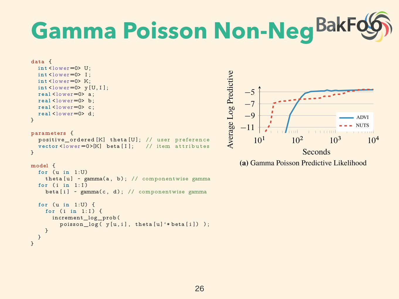
Gamma Poisson Non-Neg

26

10

110

210

310

4

�11

�9

�7

�5

SecondsAver

age

Log

Pred

ictiv

e

ADVINUTS

(a) Gamma Poisson Predictive Likelihood

10

110

210

310

4

�600

�400

�200

0

SecondsAver

age

Log

Pred

ictiv

e

ADVINUTS

(b) Dirichlet Exponential Predictive Likelihood

(c) Gamma Poisson Factors (d) Dirichlet Exponential Factors

Figure 5: Non-negative matrix factorization of the Frey Faces dataset. Comparison of �� to��: held-out predictive likelihood as a function of wall time.

Dirichlet Exponential. This is a nonconjugate Dirichlet Exponential factorization model with aPoisson likelihood. (Details in Appendix I.)

Results. Figure 5 shows average log predictive accuracy as well as ten factors recovered from bothmodels. �� provides an order of magnitude speed improvement over �� (Figure 5a). ��struggles with the Dirichlet Exponential model (Figure 5b). In both cases, �� does not produceany useful samples within a budget of one hour; we omit �� from the plots.

3.3 Scaling to Large Datasets: Gaussian Mixture Model

We conclude with the Gaussian mixture model (��) example we highlighted earlier. This is anonconjugate �� applied to color image histograms. We place a Dirichlet prior on the mixtureproportions, a Gaussian prior on the component means, and a lognormal prior on the standard devi-ations. (Details in Appendix J.) We explore the image�� dataset, which has 250 000 images [25].We withhold 10 000 images for evaluation.

In Figure 1a we randomly select 1000 images and train a model with 10 mixture components. ��struggles to find an adequate solution and �� fails altogether. This is likely due to label switching,which can a�ect ��-based techniques in mixture models [4].

Figure 1b shows �� results on the full dataset. Here we use �� with stochastic subsamplingof minibatches from the dataset [3]. We increase the number of mixture components to 30. With aminibatch size of 500 or larger, �� reaches high predictive accuracy. Smaller minibatch sizes leadto suboptimal solutions, an e�ect also observed in [3]. �� converges in about two hours.

4 Conclusion

We develop automatic di�erentiation variational inference (��) in Stan. �� leverages automatictransformations, an implicit non-Gaussian variational approximation, and automatic di�erentiation.This is a valuable tool. We can explore many models and analyze large datasets with ease. Weemphasize that �� is currently available as part of Stan; it is ready for anyone to use.

AcknowledgmentsWe thank Dustin Tran, Bruno Jacobs, and the reviewers for their comments. This work is supportedby NSF IIS-0745520, IIS-1247664, IIS-1009542, SES-1424962, ONR N00014-11-1-0651, DARPAFA8750-14-2-0009, N66001-15-C-4032, Sloan G-2015-13987, IES DE R305D140059, NDSEG,Facebook, Adobe, Amazon, and the Siebel Scholar and John Templeton Foundations.

8

data {

int < lower=0> U;

int < lower=0> I ;

int < lower=0> K;

int < lower=0> y [U, I ] ;

r ea l < lower=0> a ;

r ea l < lower=0> b ;

r ea l < lower=0> c ;

r ea l < lower=0> d ;

}

parameters {

pos i t i v e_orde r ed [K] theta [U ] ; // user p r e f e r e n c e

vector < lower =0>[K] beta [ I ] ; // item a t t r i b u t e s

}

model {

f o r (u in 1 :U)

theta [ u ] ~ gamma( a , b) ; // componentwise gamma

f o r ( i in 1 : I )

beta [ i ] ~ gamma( c , d) ; // componentwise gamma

f o r (u in 1 :U) {

f o r ( i in 1 : I ) {

increment_log_prob (

po is son_log ( y [ u , i ] , theta [ u ] ‘ * beta [ i ] ) ) ;

}

}

}

Figure 8: Stan code for Gamma Poisson non-negative matrix factorization model.

data {

int < lower=0> U;

int < lower=0> I ;

int < lower=0> K;


r ea l < lower=0> lambda0 ;

r ea l < lower=0> alpha0 ;

}

trans formed data {

vector < lower =0>[K] alpha0_vec ;

f o r ( k in 1 :K) {

alpha0_vec [ k ] < - alpha0 ;

}

}

parameters {

s implex [K] theta [U ] ; // user p r e f e r e n c e


}

model {

f o r (u in 1 :U)

theta [ u ] ~ d i r i c h l e t ( alpha0_vec ) ; // componentwise d i r i c h l e t

f o r ( i in 1 : I )

beta [ i ] ~ exponent i a l ( lambda0 ) ; // componentwise gamma

f o r (u in 1 :U) {

f o r ( i in 1 : I ) {



}

}

}

Figure 9: Stan code for Dirichlet Exponential non-negative matrix factorization model.

18

Dirichlet Exponential NonNeg

27

10

110

210

310

4

�11

�9

�7

�5

SecondsAver

age

Log

Pred

ictiv

e

ADVINUTS

(a) Gamma Poisson Predictive Likelihood

10

110

210

310

4

�600

�400

�200

0

SecondsAver

age

Log

Pred

ictiv

e

ADVINUTS

(b) Dirichlet Exponential Predictive Likelihood

(c) Gamma Poisson Factors (d) Dirichlet Exponential Factors

Figure 5: Non-negative matrix factorization of the Frey Faces dataset. Comparison of �� to��: held-out predictive likelihood as a function of wall time.

Dirichlet Exponential. This is a nonconjugate Dirichlet Exponential factorization model with aPoisson likelihood. (Details in Appendix I.)

Results. Figure 5 shows average log predictive accuracy as well as ten factors recovered from bothmodels. �� provides an order of magnitude speed improvement over �� (Figure 5a). ��struggles with the Dirichlet Exponential model (Figure 5b). In both cases, �� does not produceany useful samples within a budget of one hour; we omit �� from the plots.

3.3 Scaling to Large Datasets: Gaussian Mixture Model

We conclude with the Gaussian mixture model (��) example we highlighted earlier. This is anonconjugate �� applied to color image histograms. We place a Dirichlet prior on the mixtureproportions, a Gaussian prior on the component means, and a lognormal prior on the standard devi-ations. (Details in Appendix J.) We explore the image�� dataset, which has 250 000 images [25].We withhold 10 000 images for evaluation.

In Figure 1a we randomly select 1000 images and train a model with 10 mixture components. ��struggles to find an adequate solution and �� fails altogether. This is likely due to label switching,which can a�ect ��-based techniques in mixture models [4].

Figure 1b shows �� results on the full dataset. Here we use �� with stochastic subsamplingof minibatches from the dataset [3]. We increase the number of mixture components to 30. With aminibatch size of 500 or larger, �� reaches high predictive accuracy. Smaller minibatch sizes leadto suboptimal solutions, an e�ect also observed in [3]. �� converges in about two hours.

4 Conclusion

We develop automatic di�erentiation variational inference (��) in Stan. �� leverages automatictransformations, an implicit non-Gaussian variational approximation, and automatic di�erentiation.This is a valuable tool. We can explore many models and analyze large datasets with ease. Weemphasize that �� is currently available as part of Stan; it is ready for anyone to use.

AcknowledgmentsWe thank Dustin Tran, Bruno Jacobs, and the reviewers for their comments. This work is supportedby NSF IIS-0745520, IIS-1247664, IIS-1009542, SES-1424962, ONR N00014-11-1-0651, DARPAFA8750-14-2-0009, N66001-15-C-4032, Sloan G-2015-13987, IES DE R305D140059, NDSEG,Facebook, Adobe, Amazon, and the Siebel Scholar and John Templeton Foundations.

8

data {

int < lower=0> U;

int < lower=0> I ;

int < lower=0> K;


r ea l < lower=0> a ;

r ea l < lower=0> b ;

r ea l < lower=0> c ;

r ea l < lower=0> d ;

}

parameters {

pos i t i v e_orde r ed [K] theta [U ] ; // user p r e f e r e n c e


}

model {

f o r (u in 1 :U)

theta [ u ] ~ gamma( a , b) ; // componentwise gamma

f o r ( i in 1 : I )

beta [ i ] ~ gamma( c , d) ; // componentwise gamma

f o r (u in 1 :U) {

f o r ( i in 1 : I ) {



}

}

}

Figure 8: Stan code for Gamma Poisson non-negative matrix factorization model.

data {

int < lower=0> U;

int < lower=0> I ;

int < lower=0> K;


r ea l < lower=0> lambda0 ;

r ea l < lower=0> alpha0 ;

}

trans formed data {


f o r ( k in 1 :K) {


}

}

parameters {

s implex [K] theta [U ] ; // user p r e f e r e n c e


}

model {

f o r (u in 1 :U)

theta [ u ] ~ d i r i c h l e t ( alpha0_vec ) ; // componentwise d i r i c h l e t

f o r ( i in 1 : I )

beta [ i ] ~ exponent i a l ( lambda0 ) ; // componentwise gamma

f o r (u in 1 :U) {

f o r ( i in 1 : I ) {



}

}

}

Figure 9: Stan code for Dirichlet Exponential non-negative matrix factorization model.

18

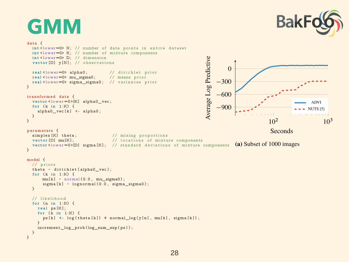
GMM

28

data {

int < lower=0> N; // number o f data po in t s in e n t i r e da ta s e t

int < lower=0> K; // number o f mixture components

int < lower=0> D; // dimension

vec to r [D] y [N ] ; // o b s e r v a t i o n s

r ea l < lower=0> alpha0 ; // d i r i c h l e t p r i o r

r ea l < lower=0> mu_sigma0 ; // means p r i o r

r ea l < lower=0> sigma_sigma0 ; // v a r i a n c e s p r i o r

}

trans formed data {


f o r ( k in 1 :K) {


}

}

parameters {

s implex [K] theta ; // mixing pr op o r t i o n s

vec to r [D] mu[K ] ; // l o c a t i o n s o f mixture components

vector < lower =0>[D] sigma [K ] ; // standard d e v i a t i o n s o f mixture components

}

model {

// p r i o r s

theta ~ d i r i c h l e t ( alpha0_vec ) ;

f o r ( k in 1 :K) {

mu[ k ] ~ normal ( 0 . 0 , mu_sigma0 ) ;

sigma [ k ] ~ lognormal ( 0 . 0 , sigma_sigma0 ) ;

}


f o r (n in 1 :N) {

r e a l ps [K ] ;

f o r ( k in 1 :K) {

ps [ k ] < - l og ( theta [ k ] ) + normal_log ( y [ n ] , mu[ k ] , sigma [ k ] ) ;

}

increment_log_prob ( log_sum_exp ( ps ) ) ;

}

}

Figure 10: advi Stan code for the gmm example.

19

10

210

3

�900

�600

�300

0

Seconds

Aver

age

Log

Pred

ictiv

e

ADVINUTS [5]


10

210

310

4

�800

�400

0

400

Seconds

Aver

age

Log

Pred

ictiv

e

B=50B=100B=500B=1000












2

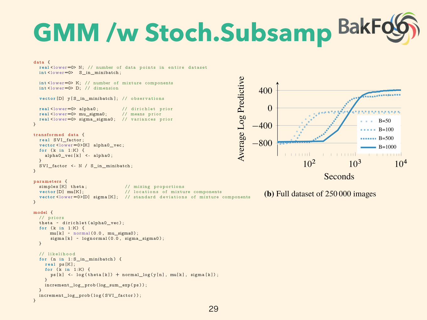
GMM /w Stoch.Subsamp

29

data {

r ea l < lower=0> N; // number o f data po in t s in e n t i r e da ta s e t

int < lower=0> S_in_minibatch ;



vec to r [D] y [ S_in_minibatch ] ; // o b s e r v a t i o n s




}

trans formed data {

r e a l SVI_factor ;


f o r ( k in 1 :K) {


}

SVI_factor < - N / S_in_minibatch ;

}

parameters {

s implex [K] theta ; // mixing pr o po r t i o n s



}

model {

// p r i o r s


f o r ( k in 1 :K) {



}


f o r (n in 1 : S_in_minibatch ) {

r e a l ps [K ] ;

f o r ( k in 1 :K) {


}


}

increment_log_prob ( l og ( SVI_factor ) ) ;

}

Figure 11: advi Stan code for the gmm example, with stochastic subsampling of thedataset.

20

10

210

3

�900

�600

�300

0

Seconds

Aver

age

Log

Pred

ictiv

e

ADVINUTS [5]


10

210

310

4

�800

�400

0

400

Seconds

Aver

age

Log

Pred

ictiv

e

B=50B=100B=500B=1000












2

Stochastic Subsampling?

30

data {

int < lower=0> N; // number o f data po in t s in e n t i r e da ta s e t



vec to r [D] y [N ] ; // o b s e r v a t i o n s




}

trans formed data {


f o r ( k in 1 :K) {


}

}

parameters {

s implex [K] theta ; // mixing pr op o r t i o n s



}

model {

// p r i o r s


f o r ( k in 1 :K) {



}


f o r (n in 1 :N) {

r e a l ps [K ] ;

f o r ( k in 1 :K) {


}


}

}

Figure 10: advi Stan code for the gmm example.

19

data {

r ea l < lower=0> N; // number o f data po in t s in e n t i r e da ta s e t

int < lower=0> S_in_minibatch ;



vec to r [D] y [ S_in_minibatch ] ; // o b s e r v a t i o n s




}

trans formed data {

r e a l SVI_factor ;


f o r ( k in 1 :K) {


}

SVI_factor < - N / S_in_minibatch ;

}

parameters {

s implex [K] theta ; // mixing pr o po r t i o n s



}

model {

// p r i o r s


f o r ( k in 1 :K) {



}


f o r (n in 1 : S_in_minibatch ) {

r e a l ps [K ] ;

f o r ( k in 1 :K) {


}


}

increment_log_prob ( l og ( SVI_factor ) ) ;

}

Figure 11: advi Stan code for the gmm example, with stochastic subsampling of thedataset.

20

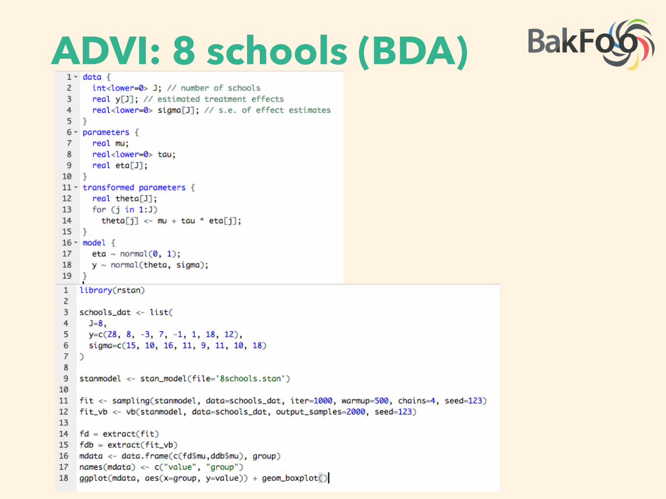
ADVI: 8 schools (BDA)

31

8 schools: result

32

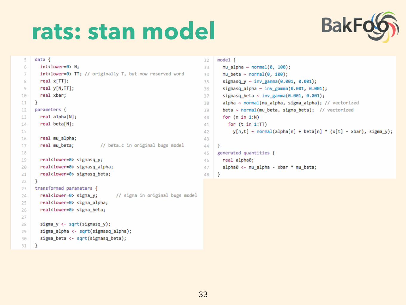
rats: stan model

33

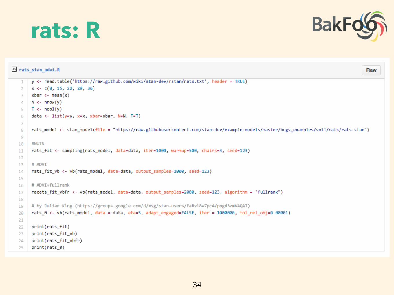
rats: R

34

rats: result

35

Very Different…

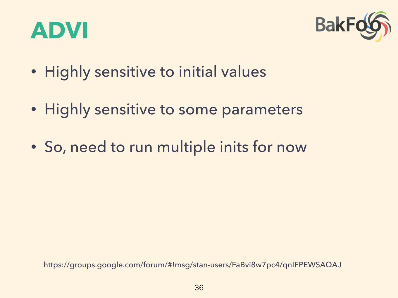
ADVI• Highly sensitive to initial values

• Highly sensitive to some parameters

• So, need to run multiple inits for now

36

https://groups.google.com/forum/#!msg/stan-users/FaBvi8w7pc4/qnIFPEWSAQAJ

Resources

Resources• ADVI - 10 minute presentation

• Variational Inference: A Review for Statisticians

• Stan Modeling Language Users Guide and Reference Manual

https://www.youtube.com/watch?v=95bpsWr1lJ8

http://www.proditus.com/papers/BleiKucukelbirMcAuliffe2016.pdf

38

https://github.com/stan-dev/stan/releases/download/v2.9.0/stan-reference-2.9.0.pdf

https://github.com/stan-dev/stan/releases/download/v2.9.0/stan-reference-2.9.0.pdf

Questions

[email protected]

39

@yutakashino

mailto:[email protected]?subject=

"automatic variational inference in stan" nips2015_yomi2016-01-20

Technology