Multimed Tools ApplDOI 10.1007/s11042-013-1707-2

Automatic tag-to-region assignment via multipleinstance learning

Zhaoqiang Xia · Yi Shen · Xiaoyi Feng · Jinye Peng ·Jianping Fan

© Springer Science+Business Media New York 2013

Abstract Translating image tags at the image level to regions (i.e., tag-to-regionassignment), which could play an important role in leveraging loosely-labeled train-ing images for object classifier training, has become a popular research topic in themultimedia research community. In this paper, a novel two-stage multiple instancelearning algorithm is presented for automatic tag-to-region assignment. The regionsare generated by performing multiple-scale image segmentation and the instanceswith unique semantics are selected out from those regions by a random walk process.The affinity propagation (AP) clustering technique and Hausdorff distance areperformed on the instances to identify the most positive instance and utilize it toinitialize the maximum searching of Diverse Density likelihood in the first stage.In the second stage, the most contributive instance, which is chosen from each bag,is treated as the key instance for simplifying the computing procedure of DiverseDensity likelihood. At last, an automatic method is proposed to discriminate theboundary between positive instances and negative instances. Our experiments onthree well-known image sets have provided positive results.

Z. Xia (B) · X. Feng · J. PengNorthwestern Polytechnical University, Xi’an, Chinae-mail: xiazhaoqiang@gmail.com

X. Fenge-mail: fengxiao@nwpu.edu.cn

J. Penge-mail: jinyepeng@nwpu.edu.cn

Y. Shen · J. FanUniversity of North Carolina at Charlotte, Charlotte, NC, USA

Y. Shene-mail: yshen9@uncc.edu

J. Fane-mail: jfan@uncc.edu

Multimed Tools Appl

Keywords Tag-to-region assignment · Multiple instance learning ·Instance identification · AP clustering

1 Introduction

With the exponential growth of digital images, there is an urgent need to achieveautomatic image annotation for supporting keyword-based (concept-based) imageretrieval [14, 27]. For the task of automatic image annotation, machine learningtechniques are usually involved to learn the classifiers from large amounts of labeledtraining images. The ground-truth labels are usually provided by professionals.Because it is time consuming and labor intensive to hire professionals for labelinglarge amounts of training images, the sizes of such professionally-labeled image setstend to be small. As a result, the classifiers, which are learned from a small set ofprofessionally-labeled training images, may hardly be generalizable. To achieve morereliable classifier training, the size of the labeled training images must be large dueto [26]: (1) the number of object classes could be very large; and (2) the learningcomplexity for some object classes could be very high because they may have largeintra-class visual diversity and inter-class visual similarity (i.e., visual ambiguity).

On the other hand, it is much easier for us to obtain large-scale loosely-labeled im-ages (object labels are loosely given at the image level rather than at the region levelor at the object level, shown in the left of Fig. 1) [11]. Such loosely-labeled imagesmay have multiple advantages: (1) they can represent various visual properties ofobject classes more sufficiently; (2) they can be obtained with less effort by providingthe object-level labels loosely at the image level rather than at the object level or atthe region level; and (3) both their labels and their visual properties are diverse, thusthey can give a real-world point of departure for object detection and scene recogni-tion. Therefore, one potential solution for the critical issue of the shortage of object-based labeled training images is to leverage large-scale loosely-labeled trainingimages for object classifier training by multiple instance learning [24, 28, 34], whereeach loosely-labeled image is considered as a bag and each region generated from theimage is treated as an instance.

It is not a trivial task to leverage the loosely-labeled images for object classifiertraining because they may seriously suffer from the critical issue of correspondence

Fig. 1 Illustration of multiple instance learning for tag-to-region assignment. The loosely-labeledimages are shown in the left

Multimed Tools Appl

uncertainty, e.g., each loosely-labeled image contains multiple image regions andmultiple object labels are given at the image level, thus the correspondences betweenthe image regions and the available labels are uncertain [15]. To leverage the loosely-labeled images for object classifier training, it is very attractive to develop new algo-rithms for: (a) supporting ambiguous image representation which can transform eachloosely-labeled image into bag of instances and expressing its semantics ambiguity(i.e., multiple labels are available for one single image) explicitly in the instancespace; (b) identifying the instance labels automatically when the labels are providedonly at the image level (i.e., loose labels); and (c) identifying the true positiveinstances fast for object classifier training.

As illustrated in Fig. 1, by assigning multiple labels (which are given at the imagelevel) into the most relevant image regions automatically, our multiple instancelearning algorithm can provide a good solution to leverage large-scale loosely-labeled images for object classifier training. Compared to the traditional multipleinstance learning algorithms, which usually label the entire tag rather than instances,a fast two-stage multiple instance learning algorithm is presented to identify the truepositive instance and can be applied to the tag-to-region assignment in this paper.Three characteristics of our proposed approach are as follows:

– Multiple-scale regions are generated by image segmentation and semanticunique instances are selected from those regions by a random walk process;

– A two-stage multiple instance learning algorithm for speeding up the DiverseDensity likelihood computation is proposed to identify the true positive in-stances;

– An automatic method of boundary demarcation is proposed to determine theboundaries of categories.

The rest of this paper is organized as follows. Section 2 reviews the related workbriefly and then the Diverse Density framework our work relied on is presented inSection 3. Section 4 introduces our new algorithm in detail and Section 5 introducesour experimental results for algorithm evaluation. We come to the conclusion andfuture work in Section 6.

2 Related work

In the last decades, many multiple instance learning algorithms have been proposedand applied to many fields since the term ‘Multiple Instance learning’ was created byDietterich et al. in a drug activity prediction domain [10]. An intuitional solution forthe multiple instance learning problem is to find the true positive instance in positivebag and many researches have been working on this. The axis-parallel rectanglelearning algorithm has been proposed to find which instances are true positive inthe positive bags directly at the instance level by Dietterich et al. [10]. The DiverseDensity approach has been proposed by Maron and Lozano-Pérez [21] and appliedto scene classification [22], which integrates all the instances in a probabilistic model.RW-SVM (Random Walk-SVM) algorithm has used a random walk process to findthe true positive instances and SVM is used to train the image classifiers to annotateentire images of three categories [31]. A multiple-task SVM algorithm, called MTS-MLMIL [26], has utilized graphic clustering to find the true positive instances and

Multimed Tools Appl

then the multi-task SVM is used to recommend tags for the image annotation. Manyother optimization algorithms, such as mi-SVM [1] and sparse-transductive SVM [2],have been proposed to identify the true positive instances through an iterativeprocedure. Another direction to solve the multiple instance learning problem is tomeasure the image at the instance level, such as Citation-kNN [32] and BAMIC [35](a multiple instance clustering algorithm). These approaches just label the entire bagwhile the preceding approaches finding the true positive instances can label bothinstances and bags. Chen et al. have developed an approach called MILES (Multiple-Instance Learning via Embedded instance Selection) to enable region-based imageannotation when labels are available only at the image level [5]. That approach mapsbags into a feature space defined by the instances and provides features for the1-norm SVM through the mapping. Vijayanarasimhan et al. have developed amultiple-label multiple-instance learning approach to achieve more effective learn-ing from loosely-labeled images [29], which uses a sparse SVM to iteratively improvepositive bags. Viola et al. [30] have transformed the traditional boosting methodsto be better suited for multiple instance learning problem and used to learn objectdetectors from loosely-labeled images.

Some approaches utilize expert-labeled training images to learn models and an-notate images through these models. A multi-class SVM algorithm has been utilizedto annotate different image regions by Cusano et al. [8]. Through statistical modelingand optimization techniques, Li and Wang [18] have developed an algorithm totrain the classifiers for hundreds of semantic concepts. A probabilistic model hasbeen proposed to estimate the mixture density for each image and minimize theannotation error by Carneiro et al. [3]. Jeon et al. utilize a cross-media relevancemodel to annotate images automatically [13]. Other approaches have been proposedto utilize the user-supported image-level tags to annotate new images. A bi-layersparse coding algorithm based on over-segmented image regions has been used toannotate images [20]. Liu et al. [16] have proposed a multi-edge graph model to labelthe regions. Yang et al. have utilized Diversity Density framework to enrich imagetags [33]. A weakly supervised graph propagation method has been developed toassign annotated labels at the image level to the semantic regions [19].

In this paper, we focus on the Diverse Density algorithm for multiple instancelearning, which has been used in many applications [5, 33]. The advantage of theDiverse Density framework is to use the statistical information of all bags in a prob-abilistic way, which accumulates the instances to the bag level to utilize the label in-formation provided. The instances are banded in the Noisy-Or probabilistic model toobtain the likelihood for all bags, however, it is difficult to solve the optimal problemif too many instances exist in the Noisy-Or model. So we propose a novel two-stageapproach based on the Diverse Density algorithm to accelerate the computation ofDiverse Density likelihood. Before introduced our approach, we revisit the DiverseDensity algorithm briefly in the next section.

3 Diverse density

Maron et al. propose the Diverse Density framework to solve the problem of drugactivity prediction and then apply it to support scene classification [21, 22]. Thegeneral framework uses the likelihood of instances being positive (i.e., Diverse

Multimed Tools Appl

Density) to measure the intersection of positive bags minus the union of negativebags. Diverse Density at a point is defined to measure how many different positivebags have instances near that point and how far the negative instances are away fromthat point [21]. The target of the Diverse Density likelihood DD(x) is to find anappropriate point (denoted as t) in the feature space which has the most true positiveinstances around that point and most true negative instances away from that point.This appropriate point t in the Diversity Density framework is also called the concept,where a bag is labeled positive even if only one of the instances in it falls withinthe concept and a bag is labeled negative only if all the instances in it are negative.The concept can be discovered through maximizing the likelihood of positive bagsand negative bags in the feature space. The appropriate point (the desired concept)corresponds to the maximum of Diverse Density likelihood in the feature space.

In the Diverse Density framework, the set of loosely-labeled images (their labelsare given at the image level or bag level) is defined as D which consists of a setof bags B = {B1,. . . , Bm} and corresponding labels L = {l1,. . . , lm}. Let bag Bi ={Bi1,. . . , Bij ,. . . Bin} where Bij is the jth instance and label li = {li1,. . . , lij ,. . . lip}where lij corresponds to the label of jth instance in Bi bag. The positive bags aredenoted as B+

i and jth instance in B+i as B+

ij . Likewise, B−ij represents a negative

instance in the negative bag B−i . The diverse density over all points x in the feature

space is denoted as DD(x) = P(x = t|B+1 , . . . , B+

n , B−1 , . . . , B−

m). The concept (thepoint t) can be found by computing maximum DD(x). Assuming that the maximumpoint t follows a uniform prior in the feature space, according to the Bayes’ rule, thisquestion can be equivalent to

arg maxx

DD(x) = arg maxx

∏

i

P(x = t|B+i )

∏

i

P(x = t|B−i ) (1)

The Diverse Density algorithm uses the Noisy-OR model to compute the probabilityof a bag being positive near the potential point t and the probability of negative bagsbeing away from the point t

P(x = t|B+i ) = 1 −

∏

j

(1 − P(x = t|B+ij ))

P(x = t|B−i ) =

∏

j

(1 − P(x = t|B−ij )) (2)

Then those probabilities are modeled by the distance between the potential target ofconcept t and the instances:

P(x = t|Bij) = exp(−‖Bij − x‖2) (3)

If the instances in a positive bag are near the potential target x, the probability P(x =t|B+

i ) would be high. Likewise, the probability P(x = t|B−i ) should be high only if the

instances in a negative bag are far away from the candidate point x. To reduce thecomplexity of the Diverse Density algorithm, the negative logarithm of DD(x) canbe adopted to search its minimum value instead of computing the DD(x) directly.

From (1), one can observe that all instances need to be integrated into the likeli-hood DD(x), thus the formula becomes very complicated in computability and doesnot have analytic solutions. Furthermore, the complexity of the generative modelis nonlinear with the number of instances and bags. The gradient ascent algorithm

Multimed Tools Appl

can be utilized to find the maximum of DD(x) even if it is not convex. To avoid thelocal maximum of DD(x), multiple initial points need to be adopted to find the globalmaximum of DD(x). So all the positive instances are used as its initial points and oneof them is likely to be close to the maximum point t. Although it is beneficial to findthe global solution for the DD(x), it is less efficient for computing through multiplestarting points especially as the number of positive instances becomes very large.Based on this observation, our proposed algorithm for multiple instance learningwill identify an instance from all these positive instances as the single initial pointrather than using all the positive instances as the initial points. On the other hand, theDD(x) is actually affected mostly by the instances which are nearest to the conceptt in each bag. Thus our proposed algorithm for multiple instance learning only usesone instance instead of all instances to compute DD(x) in each bag. Through thesetwo steps, our proposed algorithm for multiple instance learning can reduce thecomputational cost significantly and guarantee faster convergence.

4 Our proposed method

In this section, we introduce our proposed algorithm of multiple instance learning,which can be applied to solve the problem of tag-to-region assignment. Figure 2illustrates the framework of our proposed algorithm regarding the tag-to-regionassignment. Firstly, the positive bags (positive images) for a certain tag are generatedby collecting images labeled the specified tag (e.g. cow, aeroplane, or tree) whilenegative bags are generated by collecting images without that tag. Then we utilize a

Fig. 2 Illustration of our proposed algorithm for the problem of tag-to-region assignment witha multiple instance learning procedure, which includes three key components: a using the JSEGsegmentation to generate multiple-scale instances and select instances with unique semantics;b utilizing the AP clustering to choose the best candidate for Diverse Density as the single initialpoint; c speeding up the procedure of computing Diverse Density likelihood maximum by identifyingthe most contributive instance from each bag

Multimed Tools Appl

multiple instance learning framework to discover a concept and its boundary for eachtag (e.g. cow), which would be explained from Sections 4.1 to 4.5. Finally, an appro-priate tag selected from all tags would be assigned to the instance (i.e. image region)by ranking the relative distances between the instance and concepts of all tags, whichis introduced in Section 4.5.

Our proposed algorithm with multiple instance learning consists of three keycomponents as shown in Fig. 2: (a) we utilize the image segmentation technique togenerate multiple-scale regions and extract those instances with unique semantics(Section 4.1); (b) we utilize the AP clustering algorithm to find the best candidatein the semantic-unique instances for computing the maximum of Diverse Densitylikelihood (Sections 4.2 and 4.3); (c) we speed up the procedure of computing theDiverse Density likelihood maximum by identifying the most contributive instancefrom each bag (Section 4.4).

4.1 Multiple-scale instance generation

In this section, we would generate multiple-scale instances in each bag and pick outthose with unique semantics from the multiple-scale instances. These regions withunique semantics would also be referred to as good instances. For some existingmultiple instance learning algorithms, the instances are generated through the ran-domly cropped selection from images [1, 22]. Such random selection procedure couldproduce too many instances in one bag and each instance would be partly positivebecause the randomly sampled boxes in images may not contain the objects ofinterest completely. These instances produced by random selection are actually notresponsible for the bag-level tags and give rise to the non-uniqueness of semantics.Another approach to tackle the non-uniqueness problem of semantics is to utilizeautomatic image segmentation. However, over-segmentation or under-segmentationcan be easily reached by using different parameters for a segmentation algorithm. Tosolve this dilemma, we utilize a set of parameters to generate multiple segments (i.e.instances) with different sizes and shapes. We call this procedure as Multiple-ScaleInstance Generation, in which at least one of these segments can correspond to thebag-level tag and satisfy the condition of semantic uniqueness. And then a randomwalk procedure can be used to find the instances with unique semantics in each bag.

We make use of the J-images segmentation (JSEG) [9] algorithm to partition animage into a set of regions (i.e., instances), which are determined by the adjustableparameter σ = (q, m). The parameter q is denoted as the color quantization thresh-old and m represents the spatial segmentation threshold in the JSEG algorithm.1

Compared to other segmentation methods, JSEG is relatively fast to generate multi-ple instances with enough parameters. Figure 3 shows examples of JSEG segmenta-tion. All these image regions are treated as the candidates of instances with uniquesemantics while some candidates of instances generated by over-segmentation areonly fragments of instances with unique semantics. So these instances cannot beused to compute the Diverse Density likelihood. Usually, the instances with uniquesemantics would be similar with those fragments because these fragments are parts of

1http://vision.ece.ucsb.edu/segmentation/jseg/

Multimed Tools Appl

Fig. 3 Illustration of generating multiple-scale regions (four scales with dif ferent σ ) and choosinggood instances with unique semantics

instances [25]. Based on this observation, a random walk process is utilized to seekthe regions which are similar with other regions and then these regions would beselected as good instances in a bag, which usually have unique semantics.

Assuming n nodes (i.e. candidate instances or regions) exist in the random walkprocess where each node corresponds to one candidate of instances in each bag. Thenthe random walk process is formulated as

ρk+1(i) = α∑

j∈�i

ρk( j)φ(i, j) + (1 − α)ρo(i) (4)

where �i is the instance neighbor set connecting with the ith instance , ρo(i) is theinitial relevance score for the ith instance, φ(i, j) is the transition probability frominstance j to i, and α ∈ [0, 1] linearly weights two terms. The relevance score for ithinstance at the kth iteration is defined as ρk(i). The first term in (4) represents thesimilarity between the i instance and other instances.

Because multiple-scale segmentation method may generate the same (over 90 %area overlapping) instances in different scales, the initial relevance score is defined as

ρo(i) = τ(i)∑ni=1 τ(i)

(5)

Multimed Tools Appl

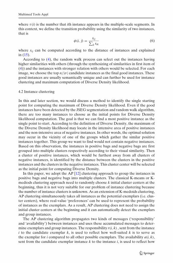
where τ(i) is the number that ith instance appears in the multiple-scale segments. Inthis context, we define the transition probability using the similarity of two instances,that is

φ(i, j) = sij∑k sik

(6)

where sij can be computed according to the distance of instances and explainedin (15).

According to (4), the random walk process can select out the instances havinghigher similarities with others (through the synthesizing of similarities in first item of(4)) and the instances with stronger relation with others would be selected. For eachimage, we choose the top n/|σ | candidate instances as the final good instances. Thesegood instances are usually semantically unique and can further be used for instanceclustering and maximum computation of Diverse Density likelihood.

4.2 Instance clustering

In this and later section, we would discuss a method to identify the single startingpoint for computing the maximum of Diverse Density likelihood. Even if the goodinstances have been detected by the JSEG segmentation and random walk algorithm,there are too many instances to choose as the initial points for Diverse Densitylikelihood computation. The goal is that we can find a most positive instance as thesingle point to start. According to the definition of Diverse Density, the maximum ofthe Diverse Density likelihood may locate in the intensive area of positive instancesand the non-intensive area of negative instances. In other words, the optimal solutionmay occur in the vicinity of one of the groups which gather the similar positiveinstances together. This group we want to find would not contain negative instances.Based on this observation, the instances in positive bags and negative bags are firstgrouped into multiple clusters respectively according to their visual similarity. Thena cluster of positive instances, which would be furthest away from all clusters ofnegative instances, is identified by the distance between the clusters in the positiveinstances and the clusters in the negative instances. This cluster center will be selectedas the initial point for computing Diverse Density.

In this paper, we adopt the AP [12] clustering approach to group the instances inpositive bags and negative bags into multiple clusters. The classical K-means or K-mediods clustering approach need to randomly choose k initial cluster centers at thebeginning, thus it is not very suitable for our problem of instance clustering becausethe number of instance clusters is unknown. As an extension of K-medoids clustering,AP clustering simultaneously takes all instances as the potential exemplars (i.e. clus-ter centers), where real-value ‘preferences’ can be used to represent the probabilityof instances as the exemplars. As a result, AP clustering does not need to assign theinitial cluster centers at the beginning and it can automatically detect the exemplarsand group instances.

The AP clustering algorithm propagates two kinds of messages (‘responsibility’and ‘availability’) between instances and uses these accumulated messages to deter-mine exemplars and group instances. The responsibility r(i, k) , sent from the instancei to the candidate exemplar k, is used to reflect how well-suited k is to serve asthe exemplar for i compared to all other possible exemplars. The availability a(i, k),sent from the candidate exemplar instance k to the instance i, is used to reflect how

Multimed Tools Appl

appropriate it would be for the instance i to select k as its exemplar, taking supportfrom other instances into account [12]. These messages are updated using the rules

r(i, k) ← s(i, k) − maxk′s.t.k′ �=k

{a(i, k′) + s(i, k′)

}

a(i, k) ← min

⎧⎨

⎩0, r(k, k) +∑

i′s.t.i′ /∈{i,k}max

{0, r(i′, k)

}⎫⎬

⎭ (7)

where s(i, k) represents the similarity between ith instance and kth instance. The self-availability is updated as follows

a(k, k) ←∑

i′s.t.i′ /∈{i,k}max{0, r(i′, k)} (8)

According to the rules above, the responsibilities are first updated when the availabil-ities a(i, k′) are initialized to zero and the availabilities are then updated when the re-sponsibilities are given. The algorithm is deemed to have converged when the updat-ing no longer change, where the entities with maximal a(k, k) in all a(i, k) are selectedas exemplars automatically. After the cluster centers are detected, the remaininginstances are assigned to their nearest cluster centers automatically. Through the APclustering, the instances from positive bags and negative bags are grouped separatelyand the similar instances are grouped into the same clusters. The selection of anoptimal initial point based on these clusters would be introduced in the next section.

4.3 Candidate identification

As discussed above, we can utilize the AP clustering to group instances into two kindsof clusters: positive clusters and negative clusters. The clusters, which are groupedfrom positive instances, are called positive clusters denoted as �; the clusters, whichare grouped from negative instances, are called negative clusters denoted as �. Afterthat, we need to find a cluster furthest away from the clusters of negative clusters� in the clusters of positive clusters �. The maximum of Diverse Density likelihooddefined in (1) may occur at the adjacent area of such cluster. So this cluster center isreferred to as the most positive instance, which can be used as the best initial pointfor the Diverse Density computation. Such a cluster can be identified by the distancebetween the positive clusters � and the negative clusters �.

In this paper, the Hausdorff distance is used to measure the distance between twoclusters (i.e., two instance sets), which has the advantage that it is not affected by amoderate number of outliers. For two instance sets Cm ∈ � and Cn ∈ �, the Haus-dorff distance between Cm and Cn is defined that each element in Cm is within Haus-dorff distance d of at least one element in Cn and each point in Cn is within Hausdorffdistance d of at least one element in Cm. The Hausdorff distance is defined as:

H(Cm, Cn) = max { h(Cm, Cn), h(Cn, Cm) }h(Cm, Cn) = max

xm∈Cm

minxn∈Cn

d(xm, xn) (9)

where the xm and xn are the elements in the instance sets Cm and Cn. The distanced(xm, xn) between two instances can be any distance metric corresponding to thefeature extraction. The distance we adopt will be introduced in details in Section 5.2.

Multimed Tools Appl

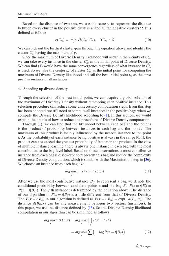
Based on the distance of two sets, we use the score γ to represent the distancebetween every cluster in the positive clusters � and all the negative clusters �. It isdefined as follows

γ (Cm) = minn

H(Cm, Cn), ∀Cm ∈ � (10)

We can pick out the furthest cluster-pair through the equation above and identify thecluster C∗

m having the maximum of γ .Since the maximum of Diverse Density likelihood will occur in the vicinity of C∗

m,we can take every instance in the cluster C∗

m as the initial point of Diverse Density.We can find (1) would have the same convergence regardless of what instance in C∗

mis used. So we take the center tm of cluster C∗

m as the initial point for computing themaximum of Diverse Density likelihood and call the best initial point tm as the mostpositive instance in all instances.

4.4 Speeding up diverse density

Through the selection of the best initial point, we can acquire a global solution ofthe maximum of Diversity Density without attempting each positive instance. Thisselection procedure can reduce some unnecessary computation steps. Even this stephas been adopted, we still need to compute all instances in the positive bags when wecompute the Diverse Density likelihood according to (1). In this section, we wouldexplain the details of how to reduce the procedure of Diverse Density computation.

Through (1), we can find that the likelihood between each bag and the point tis the product of probability between instances in each bag and the point t. Themaximum of this product is mainly influenced by the nearest instance to the pointt. As the probability of each instance being positive is always in the range [0, 1], theproduct can not exceed the greatest probability of factors in the product. In the viewof multiple instance learning, there is always one instance in each bag with the mostcontribution to the bag-level label. Based on these observations, a most contributiveinstance from each bag is discovered to represent this bag and reduce the complexityof Diverse Density computation, which is similar with the Maximization-step in [36].We choose an instance from each bag like

arg maxj

P(x = t|Bi( j)) (11)

After we use the most contributive instance Bij∗ to represent a bag, we denote theconditional probability between candidate points x and the bag Bi: P(x = t|B′

i) =P(x = t|Bij∗). The j∗th instance is determined by the equation above. The distanceof our algorithm in P(x = t|Bij) is a little different from that of Diverse Density.The P(x = t|Bij) in our algorithm is defined as P(x = t|Bij) = exp(−d(Bij, x)). Thedistance d(Bij, x) can be any measurement between two vectors (instances). Inthis paper, we use the distance defined by (15). So the Diverse Density likelihoodcomputation in our algorithm can be simplified as follows

arg maxx

DD′(x) = arg maxx

∏

i

P(x = t|B′i)

= arg minx

∑

i

(− logP(x = t|Bij)

)(12)

Multimed Tools Appl

Even if we reduce the computation steps, it is still difficult to derivate the analyticalsolution for (12). For the optimization problem above, we use the numeral solutionto search the optimal solution, where the optimal solution represents the concept ofeach tag. The method of determining the boundary for each tag would be explainedin the next section.

4.5 Boundary determination

Even if the point t in the feature space has been identified by those procedures, westill need to discover the boundary of positive instances and negative instances forautomatic tag-to-region assignment. A distance threshold T can be used to determinethe boundary. An instance is true positive if d(x, t) ≤ T; otherwise, it is negative. Thecross validation method can be used to tune this distance threshold, but even then thesearch range of validation is still too large. So we find the minimum and maximumthresholds as the upper and lower bound for searching before the cross validation isused. In the positive bags, at least one instance is positive and at most all of themare positive. According to this, we set the lower bound with the minimum distancethreshold where only one instance in a positive bag occurs and upper bound withthe maximum distance threshold where all the instances in a positive bag occur. wedefine the boundary searching range as following

Tmin = max T, d(Bij, t) ≥ T and ∃ j ∈ B+i

Tmax = min T, d(Bij, t) ≤ T and ∀ j ∈ B+i (13)

After the search range [Tmin, Tmax] has been confirmed, we adopt the K-fold (K =10) cross validation method to find the best distance threshold T ∈ [Tmin, Tmax]. Firstof all, the training set is partitioned into K subsets and one of them is alternatelyused as the validation set. In each evaluation process, we partition the search range[Tmin, Tmax] into L intervals and use the center of L intervals to validate the accuracy.The threshold which makes the best performance is then set to the final distancethreshold. The procedure of finding distance threshold is shown in Fig. 4, whichshows results for three categories of the MSRC and NUS-WIDE(OBJECT) datasets.

The concept and boundary can be used to assign the tags to regions, however, theboundaries of some categories may overlap in the feature space and one instancewould be labeled with many tags. To determine the unique categories of instances,we utilize the ranking of relative distances to solve this problem. For the concept ofith category Ci, the ranking scores of an instance are defined

γ (x) = sorti

(d(x, Ci)

Ti

)(14)

The distance measurement d(x, Ci) is computed according to (15) and Ti is the bestdistance threshold of ith category computed by cross validation. The category withthe greatest ranking score is given as the tag of this instance.

Multimed Tools Appl

Fig. 4 Threshold determination of 3 image categories on the MSRC and NUS-WIDE(OBJECT)datasets

5 Experimental evaluation

In this section, we describe the details of our experiments, including the image setswe used, the visual feature extraction of instances, the baseline methods and resultsof our experiments.

5.1 Image sets

To evaluate our algorithm precisely, different image sets are used to verify theeffectiveness of our algorithm. MSRC2 is collected from search engines, and includes591 images and 23 object categories while the ‘horse’ category is disregarded due tothe lack of examples. For average, each image has about 3.95 tags in MSRC. NUS-WIDE [6] is collected from the social website Flickr and contains 269,648 imagesand tags associated with these images originally. In our experiments, we only use thecategories which can correspond to image regions, i.e. object categories. So we pickout 25 object categories and 10,157 images (marked as NUS-WIDE(OBJECT)) toevaluate our algorithm, where each image has 2.01 tags. COREL30K [3] is based

2http://research.microsoft.com/en-us/projects/objectclassrecognition/, we use the version 2.0.

Multimed Tools Appl

on the Corel image dataset, containing 31,695 images and 1,035 tags. We processthe COREL30K dataset in the same matter that NUS-WIDE dataset is processed,and select out 27,194 images and 121 object categories3 and have enough images fortraining and testing. For each image of COREL30K, it has 2.13 tags averagely.

5.2 Visual feature

To extract effective feature from the visual content of instances, we use a well-known feature descriptor, the Bag-of-Words model with SIFT descriptor to capturekey-point information of instances [17] since the generation of good instances hasbeen introduced in Section 4. For each instance, interest points are extracted withdifference of Gaussian function and represented by a 128-dimensional descriptor.The K-means clustering is then used for constructing a code book of SIFT points.One critical issue for code book construction is to determine the size of the codebook by grid searching method. In our algorithm, we choose a codebook size of 500and represent the instance with a 500-dimensional vector.

The distance between two instances xm and xn can be measured by manyapproaches, such as Euclidean distance. However, the L1 norm (i.e. Manhattandistance) has been proved more robust to outliers than L2 norm (i.e., Euclideandistance). In this paper, we utilize the normalized L1 norm to measure the distanceof two instances. The distance function we adopted is defined as follows

d(xm, xn) =∑

i

|xm(i) − xn(i)|1 + xm(i) + xn(i)

(15)

The normalized distance measurement can reduce the impact of different dimen-sions. This distance measurement is used to compute the similarity matrix for theclustering and determine the distance boundary.

5.3 Experiments

To evaluate the performance of choosing the best initial point for computing DiverseDensity likelihood, the traditional precision and recall are used to demonstrate theeffectiveness of our clustering method. As MSRC image set provides the pixel-wiseground-truth images, we utilize these ground-truth images to test the performance ofour AP clustering. As shown in Fig. 5, precision in most categories is high, becausemost instances grouped into the same cluster are in the same category. Recall is notvery high in many categories because images in the same category are very diverse inthe visual content and not all the positive instances could be grouped into a cluster asthe members of one cluster are not infinite. When the positive instances of one cat-egory become more and more, the recall would become lower observed from Fig. 5.As the comparison of our distance measurement, we use the normalized Euclideandistance (abbreviated to ED in Fig. 5) to observe the influence of distance for cluster-ing. We can find that the distance defined in (15) can improve the precision with thecost of reducing the recall rate compared to normalized Euclidean distance observedfrom Fig. 5.

3These object categories are presented in Fig. 8 and Appendix

Multimed Tools Appl

Fig. 5 Precision and recall of AP clustering with the ground-truth of instances on the MSRC dataset

To evaluate the effectiveness of our proposed algorithm, we use the followingapproaches as the baseline algorithms: (a) our algorithm versus our approach withoutthree key components (without Multiple-scale Instances Generation, without Candi-date Identification, and without Threshold Selection); (b) our algorithm versus theDiverse Density framework [21] (using all positive instances as their initial pointsand searching the maximum Diverse Density directly); (c) our algorithm versus theEM-DD algorithm [36] (choosing all positive instances as initial points and using themost positive instance to compute the maximum Diverse Density); (d) our algorithmversus the mi-SVM algorithm [1] (an approach to find the true positive instancesusing the optimization technique directly) and (e) our algorithm versus the RW-SVM algorithm [31] (another approach to find the true positive instances usingthe random walk algorithm). For all approaches mentioned above, we compare theaccuracy and run-time of algorithms based on the MSRC, NUS-WIDE(OBJECT)and COREL30K datasets. The algorithms are executed on computer clusters withINTEL Xeon X5570 and RedHat sever 6.2. To avoid the influence of selected sam-ples, we randomly generate K different training datasets and use the average resultof these random subsets to evaluate the effectiveness of our proposed algorithm.

In order to illustrate the impact of three key components, we compare theapproaches removing those components of our approach separately. The three keycomponents contain the Multiple-scale Instances Generation (MIG), the CandidateIdentification (CI), and the Threshold Selection (TS). Observed from Table 1, itcan be concluded that the three components have different effect on the accuracy

Multimed Tools Appl

Table 1 The average accuracy/run-time of each category on three image datasets removing differentcomponents of our method

Our Method

Without MIG Without CI Without TS Overall

MSRC(%/s) 66.1/1.69 70.7/25.51 63.4/1.43 70.9/1.5NUS-WIDE(%/s) 56.9/19.38 58.0/319.44 56.1/17.48 58.1/18.1COREL30K(%/s) 53.2/14.74 54.2/247.8 52.9/14.5 54.2/14.7

of tag-to-region assignment and run-time (the run-time of learning a concept andits boundary). The components MIG and TS mainly contribute to the improvementof accuracy while the component CI contributes to the decreasing of run-time. Theprocedure MIG can select out the semantic-unique instance and be beneficial fordiscovering more accurate concept for each tag. Without the procedure MIG, someover-segmented regions (instances) may be generated and impact the detection ofconcepts for tags. Bypassing the procedure TS, the experiential threshold would betaken. Compared to utilizing the component TS, the experiential approach may besimpler but more inaccurate. The component CI is used to seek the optimal initializa-tion for computing the maximum of Diverse Density likelihood and save time of at-tempts for different initial points. The component CI utilize the clustering techniqueto discover the best initial point for computing the maximum of Diverse Densitylikelihood, instead of time-consuming computing with multiple initial points. Moredetails on the experiments are shown in Figs. 6, 7, 8 and Appendix.

To assess the advantages of the Diverse Density framework, we compare theperformance between Diverse Density-based approaches (i.e., Diverse Density,EM-DD and ours) and SVM-based algorithm (i.e., mi-SVM and RW-SVM) usingthe same three datasets and feature extraction method. As shown in Table 2, wecan observe from these results that Diverse Density-based algorithms improve theaverage accuracy for most categories. The improvement on the average accuracy ismainly attributed to the fact that Diverse Density algorithms utilize the likelihood ofinstances to reduce the ambiguity between instances (image regions) and bag-levellabels (i.e., tags of the entire image). In other words, SVM-based algorithm utilizes

Fig. 6 Average accuracy on the MSRC dataset using 8 approaches: a mi-SVM; b RW-SVM;c Diverse Density(DD); d EM-DD; e Our Method; f Our Method without MIG; g Our Methodwithout CI; h Our Method without TS

Multimed Tools Appl

Fig. 7 Average accuracy on the NUS-WIDE(OBJECT) dataset using 8 approaches: a mi-SVM;b RW-SVM; c Diverse Density(DD); d EM-DD; e Our Method; f Our Method without MIG; g OurMethod without CI; h Our Method without TS

the optimization or iteration approach to obtain the relationship between instancesand bag-level labels directly. It is difficult to achieve the target when the initial labelsare not assigned to the right instances at the starting of algorithms. Diverse Density-based algorithms are not necessary to assign the instances with right labels when thealgorithms start. In addition, the geometric shape of boundary in Diverse Densityis hypersphere in the feature space while the geometric shape of boundary in theSVM-based algorithm is hyperplane.

To illustrate the improvement of our algorithm, we compare two existing DiverseDensity-based approaches: DD and EM-DD. The average accuracy of our exper-iments using these Diverse Density algorithms in details is shown in Figs. 6, 7, 8and Appendix. The improvement of our algorithm is mainly from two components:(a) we use two steps to find the concept of each category in the feature space. TheAP clustering and Hausdorff distance between clusters are utilized to identify the

Fig. 8 Average accuracy on the 29 categories (first part of 121 categories and simultaneouslyoccurred in MSRC or NUS-WIDE) of COREL30K dataset using 7 approaches: a mi-SVM; b RW-SVM; c EM-DD; d Our Method; e Our Method without MIG; f Our Method without CI; g OurMethod without TS

Multimed Tools Appl

Table 2 Average accuracy of image annotation on three datasets using five different methods

mi-SVM (%) RW-SVM (%) DD (%) EM-DD (%) Our Method (%)

MSRC 56.6 57.8 65.8 55.2 70.9NUS-WIDE 53.2 54.1 55.6 52.8 58.1COREL30K 51.8 52.2 NR 52.5 54.2

Bold values shows the best performance

candidate exemplar of clusters as the initial point in the first step (coarse step). Fromthe initial point, the concept corresponding to each category is found by using theboosting Diverse Density procedure in the second step (fine step). (b) we designan automatic method to find the boundary for the concept after the concept hasbeen found, which is better than the method only using the leave-one-out approach.The searching range defined in (13) can avoid the over-fitting problem and speedup the searching speed. The concepts of our algorithm (maximum of DD′(x)) arealmost the same as the Diverse Density algorithm, but the mainly performancedifference between two algorithms is determined by the distance threshold selectionprocedure. We use the automatic method to find the threshold and obtain moreaccurate results. In contrast to EM-DD, our algorithm utilizes the AP clustering andHausdorff distance to find the most likely candidate in the feature space other thanrandomly choosing some initial points. Those randomly chosen points may result inthe local maximum of Diverse Density likelihood. EM-DD also uses the leave-one-out approach to obtain the boundary which may generate the over-fitting problem.Our algorithm utilizes the AP clustering and Hausdorff distance to find the concept(the point t) approximately and Diverse Density to obtain the exact concepts, andthen detect the boundary to recognize the new instances.

In Table 2, the average accuracy of each category is shown on the three datasets.The average accuracy illustrates that our algorithm obtains the best performancetotally and most categories on the three datasets while other algorithms have betterperformance than our algorithm in some categories, for instance, the ‘face’ categoryfor Diverse Density algorithm. Our experiments also show that the NUS-WIDE(OBJECT) and COREL30K image dataset are much noisier than the MSRC datasetbecause the average results of five algorithms on MSRC are better than the NUS-WIDE(OBJECT) and COREL30K datasets totally. We cannot find the optimal so-lution in most categories on COREL30K dataset using the Diverse Density methodbecause there are too many positive instances to compute the Diverse Densitylikelihood. So we cannot acquire the results on COREL30K with the Diverse Densitymethod (indicated by ‘NR’ in Table 2).

The run-time of four algorithms compared in our experiments are shown in theTable 3. The mi-SVM obtains the best run-time performance because many special

Table 3 The average run-time of each category on three image datasets using different methods

mi-SVM RW-SVM DD EM-DD(50 %) Our Method

100 200 300

MSRC(s) 1.05 1.95 3.12 6.37 780.6 257.1 1.5NUS-WIDE(s) 12.6 22.8 42.6 100.8 9829.8 3686.33 18.6COREL30K(s) 10.2 23.4 32.5 65.9 NR 135.6 14.7

Bold values shows the best performance

Multimed Tools Appl

Fig. 9 The examples of tag-to-region assignment results. Three rows are from MSRC, NUS-WIDE(OBJECT) and COREL30K datasets respectively

solution algorithms for SVM4 have been designed [23] while the DiverseDensity-based algorithms need to compute the Diverse Density maximum using thenumerical approaches, such as Newton method [7]. We choose the best initial point(i.e., most positive instance) by the clustering and Hausdorff distance to replacethe multiple initial point trial in DD and EM-DD, and use the most contributiveinstance of each bag to compute the Diverse Density instead of using all instances.So the run-time can be reduced very much. In all algorithms, the mi-SVM algorithmuses the least run-time compared to other methods, however, mi-SVM can hardlyconverge the stable solution so we set the limited iterative times for terminating thealgorithm manually, such as 100, 200 and 300 in Table 3. The run-time used by EM-DD algorithm is also determined by the number of initial instances. Although we doexperiments with different number of initial points for the EM-DD algorithm, weonly display the run-time using 50 % of positive instances which can make the bestperformance.

At last, we show some results of tag-to-region assignment experiments in Fig. 9.In the images of Fig. 9, the instance-level annotation is shown in the segmentedimages directly. Some instances (image regions) are not assigned with any tags asif the ranking scores defined in (14) are larger than 1.0. In other words, the instancedoes not belong to any category if all the scores γ (x) > 1.0.

6 Conclusion and future work

In this paper, a novel multiple instance learning algorithm is developed to speedup the procedure of Diverse Density likelihood computation, which is used forautomatic tag-to-region assignment. First of all, we utilize the JSEG image segmen-tation to generate multi-scale regions and choose the good instance in each bagby a random walk process. Then the AP clustering technique is performed on theinstances of positive bags and negative bags to identify the best initial point and

4The LIBSVM [4] is used as SVM implementation included in mi-SVM and RW-SVM.

Multimed Tools Appl

initialize the maximum searching of the Diverse Density likelihood. To recognizewhich instances are positive given a category, we propose an automatic method todetermine the boundary of categories. Our experiments on three well-known imagesets have provided very positive results. For the synonymy tags and co-occurred tags,the performance of our proposed approach would be degraded. For instance, thewords ‘car’ and ‘automobile’ cannot be distinguished very easily.

In the future, we will extend our work in two directions: (a) testing our proposedalgorithm on large-scale image sets with large-scale categories (object classes); (b)utilizing the relationship between the tags to achieve more effective solution formultiple instance learning.

Acknowledgements The authors would like to thank Jonathan Fortune for language polish. Thiswork is partly supported by the doctorate foundation of Northwestern Polytechnical University(No: CX201113), Doctoral Program of Higher Education of China (Grant No.20106102110028and 20116102110027) and National Science Foundation of China (under Grant No.61075014 and61272285).

Appendix: The part 2 and 3 of experiments on COREL30K

Fig. 10 Average accuracy on the 92 categories (part 2 and 3 of 121 categories) of COREL30K datasetusing 7 approaches: a mi-SVM; b RW-SVM; c EM-DD; d Our Method; e Our Method without MIG;f Our Method without CI; g Our Method without TS

Multimed Tools Appl

References

1. Andrews S, Tsochantaridis I, Hofmann T (2002) Support vector machines for multiple-instancelearning. Adv Neural Inf Proc Syst 15:561–568

2. Bunescu R, Mooney R (2007) Multiple instance learning for sparse positive bags. In: Proceedingsof the 24th International Conference on Machine Learning (ICML), pp 105–112

3. Carneiro G, Chan A, Moreno P, Vasconcelos N (2007) Supervised learning of semantic classesfor image annotation and retrieval. IEEE Trans Pattern Anal Mach Intell29(3):394–410

4. Chang CC, Lin CJ (2011) LIBSVM: a library for support vector machines. ACM Trans IntellSyst Technol 2:27:1–27:27

5. Chen Y, Bi J, Wang J (2006) Miles: multiple-instance learning via embedded instance selection.IEEE Trans Pattern Anal Mach Intell 28(12):1931–1947

6. Chua T, Tang J, Hong R, Li H, Luo Z, Zheng Y (2009) Nus-wide: a real-world web imagedatabase from National University of Singapore. In: Proceeding of the ACM internationalconference on image and video retrieval, p 48

7. Coleman TF, Li Y (1996) An interior trust region approach for nonlinear minimization subjectto bounds. SIAM J Optim 6(2):418–445

8. Cusano C, Ciocca G, Schettini R (2004) Image annotation using svm. In: Society of Photo-OpticalInstrumentation Engineers conference (SPIE), vol 5304, pp 330–338

9. Deng Y, Manjunath B, Shin H (1999) Color image segmentation. In: IEEE computer societyconference on Computer Vision and Pattern Recognition (CVPR), vol 2

10. Dietterich T, Lathrop R, Lozano-Pérez T (1997) Solving the multiple instance problem with axis-parallel rectangles. Artif Intell 89(1–2):31–71

11. Fan J, Shen Y, Zhou N, Gao Y (2010) Harvesting large-scale weakly-tagged image databasesfrom the web. In: IEEE computer society conference on Computer Vision and Pattern Recogni-tion (CVPR), pp 802–809

12. Frey B, Dueck D (2007) Clustering by passing messages between data points. Science315(5814):972

13. Jeon J, Lavrenko V, Manmatha R (2003) Automatic image annotation and retrieval usingcross-media relevance models. In: Proceedings of the 26th annual international ACM SIGIRconference on research and development in informaion retrieval, pp 119–126

14. Lew M, Sebe N, Djeraba C, Jain R (2006) Content-based multimedia information retrieval: stateof the art and challenges. ACM Trans Multimed Comput Commun Appl (TOMCCAP) 2(1):1–19

15. Liu D, Hua X, Zhang H (2011) Content-based tag processing for internet social images. Mul-timed Tools Appl 51:723–738

16. Liu D, Yan S, Rui Y, Zhang H (2010) Unified tag analysis with multi-edge graph. In: Proceedingsof the international conference on Multimedia (ACM MM), pp 25–34

17. Li F, Fergus R, Torralba A (2007) Recognizing and learning object categories. cvpr 2007 shortcourse

18. Li J, Wang J (2008) Real-time computerized annotation of pictures. IEEE Trans Pattern AnalMach Intell 30(6):985–1002

19. Liu S, Yan S, Zhang T, Xu C, Liu J, Lu H (2012) Weakly-supervised graph propagation towardscollective image parsing. IEEE Trans Multimedia 14(2):361–373

20. Liu X, Cheng B, Yan S, Tang J, Chua T, Jin H (2009) Label to region by bi-layer sparsity priors.In: Proceedings of the 17th ACM international conference on multimedia, pp 115–124

21. Maron O, Lozano-Pérez T (1998) A framework for multiple-instance learning. In: Advances inneural information processing systems, pp 570–576

22. Maron O, Ratan A (1998) Multiple-instance learning for natural scene classification. In: Proceed-ings of the fifteenth international conference on machine learning, vol 15, pp 341–349

23. Platt J, et al (1998) Sequential minimal optimization: a fast algorithm for training support vectormachines. Technical report msr-tr-98-14, Microsoft Research

24. Qi G, Hua X, Rui Y, Mei T, Tang J, Zhang H (2007) Concurrent multiple instance learning forimage categorization. In: IEEE conference Computer Vision and Pattern Recognition (CVPR),pp 1–8

25. Russell B, Freeman W, Efros A, Sivic J, Zisserman A (2006) Using multiple segmentations todiscover objects and their extent in image collections. In: IEEE computer society conference onComputer Vision and Pattern Recognition (CVPR), pp 1605–1614

26. Shen Y, Fan J (2010) Leveraging loosely-tagged images and inter-object correlations for tagrecommendation. In: Proceedings of the international conference on Multimedia (ACM MM),pp 5–14

Multimed Tools Appl

27. Smeulders A, Worring M, Santini S, Gupta A, Jain R (2000) Content-based image retrieval atthe end of the early years. IEEE Trans Pattern Anal Mach Intell 22(12):1349–1380

28. Tang J, Hong R, Yan S, Chua T, Qi G, Jain R (2011) Image annotation by knn-sparse graph-based label propagation over noisily tagged web images. ACM Trans Intell Syst Technol2(2):14

29. Vijayanarasimhan S, Grauman K (2008) Keywords to visual categories: multiple-instance learn-ing for weakly supervised object categorization. In: IEEE conference Computer Vision andPattern Recognition (CVPR), pp 1–8

30. Viola P, Platt J, Zhang C (2006) Multiple instance boosting for object detection. Adv Neural InfProc Syst 18:1417

31. Wang D, Li J, Zhang B (2006) Multiple-instance learning via random walk. In: Machine learning:ECML 2006, pp 473–484

32. Wang J, Zucker J (2000) Solving the multiple-instance problem: a lazy learning approach.In: Proc. 17th international conf. on machine learning, pp 1119–1125

33. Yang K, Hua X, Wang M, Zhang H (2011) Tag tagging: towards more descriptive keywords ofimage content. IEEE Trans Multimedia 13(4):662–673

34. Zha Z, Hua X, Mei T, Wang J, Qi G, Wang Z (2008) Joint multi-label multi-instance learning forimage classification. In: IEEE conference Computer Vision and Pattern Recognition (CVPR),pp 1–8

35. Zhang M, Zhou Z (2009) Multi-instance clustering with applications to multi-instance prediction.Appl Intell 31(1):47–68

36. Zhang Q, Goldman S (2001) Em-dd: an improved multiple-instance learning technique. AdvNeural Inf Proc Syst 14:1073–1080

Zhaoqiang Xia is a PhD student at Northwestern Polytechnical University. His research interestsinclude multimedia retrieval, statistical machine learning and computer vision.

Multimed Tools Appl

Yi Shen is a PhD student at University of North Carolina at Charlotte. His research interests includemulti-label learning and multiple-instance learning.

Xiaoyi Feng is a professor at Northwestern Polytechnical University. Her research interests includecomputer vision, image process, radar imagery and recognition.

Jinye Peng is a professor at Northwestern Polytechnical University. His research interests includecomputer vision, pattern recognition and signal processing.

Multimed Tools Appl

Jianping Fan is a professor at University of North Carolina at Charlotte. His research interestsinclude semantic image and video analysis, computer vision, cross-media analysis, and statisticalmachine learning.