Special Issue on CAD/Graphics 2015

Automatic reconstruction of parametric building models from indoorpoint clouds

Sebastian Ochmann n, Richard Vock, Raoul Wessel, Reinhard KleinInstitute of Computer Science II, University of Bonn, Germany

a r t i c l e i n f o

Article history:Received 7 April 2015Received in revised form11 July 2015Accepted 12 July 2015Available online 22 July 2015

Keywords:Indoor scene reconstructionPoint cloud processingParametric models

a b s t r a c t

We present an automatic approach for the reconstruction of parametric 3D building models from indoorpoint clouds. While recently developed methods in this domain focus on mere local surfacereconstructions which enable e.g. efficient visualization, our approach aims for a volumetric, parametricbuilding model that additionally incorporates contextual information such as global wall connectivity. Incontrast to pure surface reconstructions, our representation thereby allows more comprehensive use:first, it enables efficient high-level editing operations in terms of e.g. wall removal or room reshapingwhich always result in a topologically consistent representation. Second, it enables easy taking ofmeasurements like e.g. determining wall thickness or room areas. These properties render ourreconstruction method especially beneficial to architects or engineers for planning renovation orretrofitting. Following the idea of previous approaches, the reconstruction task is cast as a labelingproblem which is solved by an energy minimization. This global optimization approach allows for thereconstruction of wall elements shared between rooms while simultaneously maintaining plausibleconnectivity between all wall elements. An automatic prior segmentation of the point clouds into roomsand outside area filters large-scale outliers and yields priors for the definition of labeling costs for theenergy minimization. The reconstructed model is further enriched by detected doors and windows. Wedemonstrate the applicability and reconstruction power of our new approach on a variety of complexreal-world datasets requiring little or no parameter adjustment.& 2015 The Authors. Published by Elsevier Ltd. This is an open access article under the CC BY-NC-ND

license (http://creativecommons.org/licenses/by-nc-nd/4.0/).

1. Introduction

Digital 3D building models are increasingly used for diversetasks in architecture and design such as construction planning,visualization, navigation, simulation, facility management, renova-tion, and retrofitting. Especially for legacy buildings, suitablemodels are usually not available from the initial planning. Pointcloud measurements are often used as a starting point forgenerating 3D models in architectural software. But despite fastscanning devices and modern software, the generation of modelsfrom scratch still are largely manual and time-consuming taskswhich make automatic reconstruction methods highly desirable.

Reconstruction of indoor environments poses specific chal-lenges due to complex room layouts, clutter and occlusions.Furthermore, planning and maintenance tasks often require mod-els which give deeper insight into a building's structure on thelevel of building elements such as walls, and their relations likewall connectivity. This enables high-level editing for prototypingplanned changes and simulations requiring information like room

neighborhood or wall thickness. While previous reconstructionmethods are able to faithfully recover partially observed surfacesfrom indoor point clouds and generate accurate boundary repre-sentations in the form of mesh models, a plausible decompositioninto parametric, globally interrelated, volumetric building ele-ments yet remained an open challenge. Existing approaches eitherrepresent walls, floors and ceilings as sets of unconnected planarstructures detected in the point cloud [13,1,15,21,7] (Fig. 1(a)), oras collections of closed 3D boundaries of either the whole building[12], or separate rooms [4,19,18,8] (Fig. 1(b)). While the method in[20] reconstructs volumetric walls, their thickness is definedmanually instead of being estimated from the input data.

To overcome the limitations of previous approaches, we pro-pose a novel reconstruction method in which the representation ofbuildings using parametric, interrelated, volumetric elements(Fig. 1(c)) is an integral component. Our approach automaticallyreconstructs walls between adjacent rooms from opposite wallsurfaces observed in the input data while simultaneously takinginto account globally plausible connectivity of all elements.Together with a faithful estimation of wall thickness, the resultis a high-level editable model of volumetric wall elements. Thereconstruction is formulated as an energy minimization problemwhich simultaneously optimizes costs for assigning rooms to areal

Contents lists available at ScienceDirect

journal homepage: www.elsevier.com/locate/cag

Computers & Graphics

http://dx.doi.org/10.1016/j.cag.2015.07.0080097-8493/& 2015 The Authors. Published by Elsevier Ltd. This is an open access article under the CC BY-NC-ND license (http://creativecommons.org/licenses/by-nc-nd/4.0/).

n Corresponding author.E-mail address: ochmann@cs.uni-bonn.de (S. Ochmann).

Computers & Graphics 54 (2016) 94–103

regions of the building, and costs for separating adjacent rooms byvolumetric wall elements. In contrast to previous approaches, thishas the advantage that reasonable binary costs for the assignmentof pairs of room labels to adjacent areal regions of the building –

and thus the selection of suitable wall elements – is directlyincorporated into the global optimization. To make our methodrobust against large-scale clutter outside the building, outliers areautomatically filtered prior to reconstruction. Finally, doors andwindows are detected, classified and assigned to the respectivewall elements to further enrich the model. Our evaluation usingvarious real-world indoor scans shows that our method rapidlyprovides models which can be used for e.g. planning of retrofitting,especially since our method requires little or no parameteradjustment.

Applications: The distinguishing feature of our approach is thatit directly captures important properties and relations of buildingelements. Since architectural Building Information Modeling (BIM)formats (e.g. Industry Foundation Classes, IFC) are based on similarrelational paradigms, exporting our results to architectural soft-ware is straight forward. This enables a whole range of processingand analysis tasks in industry-standard software. We exemplifysome applications for e.g. planning of retrofitting in Fig. 2 whichcan directly be implemented using our results: since the incidenceand adjacency relations of walls and rooms are inherently known,selecting e.g. all walls enclosing a room or manipulating wholewalls while maintaining overall room topology is easily possible(Fig. 2(a)). This allows for quick, high-level prototyping of changeson the level of semantically meaningful construction elementgroups. The available information also enables more complexqueries for e.g. the subset of wall elements that are simultaneouslyincident to two adjacent rooms (Fig. 2(b)). Together with directlyavailable properties like wall thickness, openings, room and wallareas, this provides important information for performing acousticor thermal simulations. The global connectivity informationfurther allows us to perform pathfinding in the whole buildingstory (Fig. 2(c)) for e.g. simulating and optimizing escape routes.

2. Related work

Okorn et al. [13] generate 2D floor plans from 3D point clouds.A histogram of the vertical positions of all measured points is built.Peaks in this histogram are considered to be large horizontalplanar structures (i.e. floor and ceiling surfaces). After removingpoints belonging to the detected horizontal structures, a linefitting on the remaining points is performed. The resulting linesegments constituting the floor plan are not connected and do notprovide e.g. closed boundaries of rooms. Budroni and Boehm [4]extract planar structures for floors, ceilings and walls by conduct-ing a plane sweep. Using a piecewise linear partitioning of the x–y-plane, they classify cells of this partitioning as inside and outsideby determining the occupancy of the cells by measured points andconsidering densely occupied cells as inside. The result is a 2.5Dextrusion of the determined room boundary. In the approach bySanchez and Zakhor [15], points are classified into floor, ceiling,wall, and remaining points using the point normal orientations.For floor, ceiling and wall points, planar patches are fitted andtheir extents are estimated using alpha shapes. Parametric stair-case models are fitted to the set of remaining points. The resultingmesh models consist of unconnected planar surfaces. Monszpartet al. [7] propose a method for extracting planar structures in pointclouds which follow regularity constraints. Their optimizationapproach balances data fitting and simplicity of the resultingarrangement of planes. A method for generating visually appealingindoor models is proposed by Xiao and Furukawa [20]. An inverse-CSG approach is used for reconstructing the building's geometryby detecting planar structures and then fitting cuboid primitives.These primitives are combined using CSG operations; the qualityof the resulting model is tested using an energy functional. Finally,the resulting mesh model is textured using captured images. Adrawback is that the building needs to be sufficiently wellapproximated by the used cuboid primitives. Adan and Huber [1]reconstruct planar floor, ceiling, and wall surfaces frommulti-storypoint clouds by first detecting the modes of a histogram of point

Fig. 1. Schematic of editing capabilities of different kinds of reconstructions. The input point cloud is shown on the left. The remaining columns exemplify editing operations,i.e. elements are moved in the directions of the arrows. Surface representations without (column (a)) or with (column (b)) connectivity information do not allow intuitiveediting on the level of wall elements. Our reconstruction (column (c)) maintains room topology and global wall connectivity.

Fig. 2. Example operations which are easily implemented using our results. (a) Relations between walls and rooms enable editing while maintaining room topology. Notehow incident walls are adjusted automatically. (b) Automatic determination of wall elements shared between rooms together with automatic measurements enable e.g.acoustic or thermal simulations. (c) Global connectivity enables pathfinding for e.g. simulation and optimization of escape routes.

S. Ochmann et al. / Computers & Graphics 54 (2016) 94–103 95

height values to find horizontal planes, and then detecting verticalplanes by means of Hough transform. They recover occluded partsof reconstructed surfaces and perform an opening detection bymeans of Support Vector Machine (SVM) learning. Xiong et al. [21]extend this approach by classifying detected planar patches asfloor, ceiling, wall or clutter using a stacked learning approach,also taking into account contextual information of neighboringpatches. Mura et al. [8] reconstruct indoor scenes with arbitrarywall orientations by building a 3D Delaunay tetrahedralization ofthe input dataset and partitioning inside and outside using adiffusion process governed by affinities of tetrahedron pairs. Abinary space partitioning is also done by Oesau et al. [12] by firstsplitting the input dataset horizontally at height levels of highpoint densities and then constructing 2D arrangements of projec-tions of detected wall surfaces. The space partitioning into insideand outside is performed by means of Graph-Cut. Otherapproaches not only perform binary space partitioning but labeldifferent rooms: Turner and Zakhor [19] generate 2.5D watertightmeshes by first computing an inside/outside labeling of a trian-gulation of wall points and a subsequent partitioning into separaterooms using a Graph-Cut approach. This method is further devel-oped by Turner et al. in [18], improving the texture mappingcapabilities of the algorithm. The results are well-regularized,watertight, textured mesh models. Mura et al. [9] first extractcandidate wall elements while taking into account possiblyoccluded parts of the surfaces to determine the real wall heightsfor filtering out invalid candidates. After constructing a 2D linearrangement, they use a diffusion embedding to establish a globalaffinity measure between faces of the arrangement, and determineclusters of faces constituting rooms. The result is a labeledboundary representation of the building's rooms. Many of thesemethods build upon a spatial partitioning defined by detected wallsurfaces and a subsequent classification of regions of this parti-tioning. Although the resulting models have applications likevisualization, navigation or energy monitoring [17], they do notrealize a reconstruction of volumetric, interconnected buildingelements like walls.

3. Approach

The starting point of our approach is a registered point cloud ofone building story consisting of multiple indoor scans includingscanner positions. Registration is usually done using the scannersoftware and is outside the scope of this paper. The unit ofmeasurement and up direction are assumed to be known. Surfacenormals for each point are estimated.

We argue that the wall structure of most building stories can berepresented as a piecewise-linear, planar graph in which edgesrepresent wall elements and vertices are locations where walls areincident (Fig. 3(e)). Wall thickness is a scalar edge attribute.Conversely, faces of this graph represent the spatial room layout.There obviously exists a duality between the story's room layoutand its wall constellation, i.e. one representation can directly bederived from the other. The main idea of our approach is that –

while both representations are essentially equally hard to recon-struct – we can derive important hints (priors) for the room layoutfrom indoor point cloud scans since they are a sampling of theinner surfaces of room volumes. It is therefore meaningful to baseour reconstruction on the derivation of a suitable room layoutfrom which the constellation of walls is immediately obtained dueto the duality.

We extract priors for the room layout as follows: assuming thateach room was scanned from one position (or few positions),separate scans yield a coarse segmentation of the point cloud intoseparate rooms (Fig. 3(a)). We improve this segmentation using a

diffusion process which eliminates most overlapping regionsbetween scans (Fig. 3(b)) and automatically filters out clutteroutside of the building. As further described below, the determi-nation of a suitable room layout is then formulated as a labelingproblem of the regions of a suitable partitioning of the horizontalplane (using labels for different rooms and the outside area). Thisdirectly follows the aforementioned duality principle: after deter-mining a suitable labeling, connected components of identicallylabeled cells are rooms, and edges separating differently labeledregions are wall elements.

Since our goal is to extract a piecewise-linear graph of walls, weconstruct a partitioning based on potential wall surfaces: we firstdetect vertical planes as candidates for wall surfaces and projectthem to the horizontal plane (Fig. 3(c)). Similar to previousapproaches [9,11,12] we then construct an arrangement of (infi-nitely long) lines from the set of possible wall surfaces (Fig. 3(d)).In contrast to previous approaches, edges of this arrangementrepresent wall centerlines instead of wall surfaces. Furthermore,arrangement lines are not only constructed from single wallsurfaces but also from pairs of parallel surfaces which yieldcandidates for walls separating adjacent rooms. This subtle butcrucial difference allows us to go beyond the reconstruction ofseparate room volumes as done in previous works (Fig. 1(b)) byenabling the algorithm to reconstruct room-separating wall ele-ments directly. In order to guide the selection of adequate wallelements, we retain the information from which supportingmeasured points each edge originates. This yields wall selectionpriors encouraging the reconstruction of wall elements whichwere constructed from surfaces belonging to the same pair ofrooms that the wall separates.

The determination of a globally plausible labeling is then formu-lated as an energy minimization problem. This allows us to incorpo-rate room layout priors and wall selection priors as unary and binarycosts into one optimization. After an optimal labeling has beendetermined, only retaining edges separating differently labeledregions are the sought wall structures (Fig. 3(e)). Extruding wallsaccording to estimated room heights and a detection and classificationof openings yields the final parametric model (Fig. 3(f)).

4. Point cloud segmentation

To obtain priors for the localization of rooms in subsequentsteps, each point of the input point cloud is automatically assigneda label for a room or the outside area. Our approach is based on themethod by Ochmann et al. [10] which we will briefly summarizebefore describing our modifications: the original method assumesat least one scan within each room; multiple scans per room aremerged manually such that a one-to-one mapping between(merged) scans and rooms is obtained. The initial assignment ofeach point to one of the (merged) scans (Fig. 3(a)) provides acoarse segmentation of the point cloud into rooms. However,openings such as open doors lead to severe overlaps betweenscans, causing large areas of the point cloud to contain a mix ofdifferently labeled points. To obtain a point labeling that roughlycorresponds to the building's room layout and is homogeneouswithin each room (Fig. 3(b)), an automatic labeling refinement isperformed. The process is based on the assumption that mostpoints that are visible from the position of a point p are alreadylabeled correctly. By determining which points are visible from theposition of p and averaging the observed labels, a new (soft)labeling of p is obtained. After iterating this procedure, the labelwith the highest confidence is assigned to p. This process can beinterpreted as a diffusion of point labels between points governedby mutual visibility. In practice, a stochastic ray casting from the

S. Ochmann et al. / Computers & Graphics 54 (2016) 94–10396

position of p into the hemisphere around the normal of p isperformed.

We extend this method in two ways: first, we automaticallyfilter out clutter outside of the building which is often caused bywindows or mirrors. We argue that for a point p that is part ofclutter outside of the building, most rays cast from p into thehemisphere around the normal of p do not hit any interior wallsurfaces. In this case we assign a high value for an additionaloutside label to p. This modification proves to be highly effective inour experiments as demonstrated in Fig. 3(b) (gray points havebeen assigned the outside label). Second, we do not require thatmultiple scans per room are merged manually. Instead, we run thereconstruction using all scans as separate labels. In case of multi-ple scans in a room, this leads to implausible walls within roomswhich are subsequently removed as described in Section 7.

5. Generation of wall candidates

Candidates for wall elements are derived from vertical surfacesobserved in the scans. They constitute possible locations of wallsfor the optimization in Section 6. Since wall heights and lengthsare not regarded in this step, the following 2D representation isused: each wall candidate w¼ ðtw;nw; dwÞ is defined by a thicknesstwAR⩾0 and an infinite centerline in the horizontal plane given inHesse normal form ⟨nw; x⟩�dw ¼ 0. Wall heights and lengths willbe determined later.

In a first step, planes in the 3D point cloud are detected using aRANSAC implementation by Schnabel et al. [16]. Nearly verticalplanes ð711Þ with a sufficiently large approximate area ð⩾1:5 m2Þare considered as potential wall surfaces. For a plane P fulfillingthese constraints, let nPAR3 be the plane normal and PP the set of

measured points supporting P. Each extracted plane P is trans-ferred to the horizontal plane as a wall surface line lP defined by⟨nlP ; x⟩�dlP ¼ 0. A schematic example for the extraction of wallsurface lines is shown in Fig. 4(a)–(c). The normal nlP is approxi-mated by the projection of nP into the horizontal plane,

nlP : ¼ ððnPÞx; ðnP ÞyÞ‖ððnPÞx; ðnP ÞyÞ‖2

:

The distance to the origin dlP is determined by least squares fittingto the set Pxy

P of support points projected to the horizontal planeusing the fixed normal nlP such that

PpAPxy

Pð⟨nlP ; p⟩�dlP Þ2 is

minimized. From the wall surface lines, we then generate twokinds of wall candidates as we do not know at this point whichtypes of candidates will yield a globally plausible reconstruction:

Outside walls: For each single wall surface line lP , we construct acandidate for a wall separating a room from the outside area(Fig. 4(d)). Since the real wall thickness cannot be determinedautomatically from a single surface, a user-specified thickness isused (in our experiments, tw ¼ 20 cm). The centerline of thecandidate is constructed such that the side of the wall candidatethat points towards the inside of the room is identical to lP , i.e. thecenterline is defined by ⟨nlP ; x⟩�dw ¼ �tw=2.

Room-separating walls: To generate candidates for walls separ-ating adjacent rooms, each pair of wall surface lines fulfillingcertain constraints is considered as two opposite surfaces of a wallseparating adjacent rooms (Fig. 4(e)). Let lP1 and lP2 be two wallsurface lines that are approximately parallel ð711Þ and haveopposing normal orientations. To prune invalid pairs, a coarsecheck is performed whether the projected support pointsets of theoriginating planes Pxy

P1; Pxy

P2(partially) overlap. To this end, the

support pointsets are projected onto the respective opposite line.If support points are present near the projected points, their

Fig. 3. Overview of our approach (see also Section 3). (a) Input point cloud; assignment of points to scans shown in different colors. (b) Refined assignment after automaticsegmentation. (c) Detected vertical planes transferred to the horizontal plane. (d) Candidates for walls are derived from single and pairs of projected planes. Intersecting theircenterlines yields a planar graph whose faces are subsequently assigned labels for rooms or outside area. (e) Only edges separating differently labeled faces are retained.(f) The final model with detected and classified wall openings, e.g. doors (green) and windows (yellow). (For interpretation of the references to color in this figure caption,the reader is referred to the web version of this paper.)

Fig. 4. Wall candidate generation. (a) and (b) Detected vertical planes in the 3D point cloud are projected into the horizontal plane. (c) Different wall surface lines includingthe respective (projected) support points and surface normals. (d) For each single wall surface, an infinitely long wall candidate w for a wall separating a room from outsidearea is generated. In this case, the thickness tw is user-specified. (e) For each pair of approximately parallel wall surfaces, a candidate for separating adjacent rooms isgenerated. In this case, wall thickness is estimated from the data.

S. Ochmann et al. / Computers & Graphics 54 (2016) 94–103 97

support is considered overlapping. For each pair fulfilling theseconstraints, a wall candidate is generated by fitting to lP1 and lP2

simultaneously: The candidate's normal nw is first determined asthe average of the normals n1;n2 of lP1 ; lP2 , weighted with thecardinality of the support pointsets,

nw : ¼ jPxyP1jn1þjPxy

P2j ð�n2Þ

J ðjPxyP1jn1þjPxy

P2j ð�n2ÞÞJ2

:

Using the common normal nw, two parallel lines li; iAf1;2gdefined by ⟨nw; x⟩�di ¼ 0 are fitted to the respective supportpointsets such that

PpAPxy

Pið⟨nw; p⟩�diÞ2 is minimized. The center-

line of the wall candidate is constructed midway between theparallel lines, ⟨nw; x⟩�1

2 ðd1þd2Þ ¼ 0, and the candidate's thicknessis defined as the distance between them, tw ¼ jd1�d2 j . Candi-dates with a thickness above a threshold are discarded (in ourexperiments, tw460 cm).

6. Determination of an optimal room and wall layout

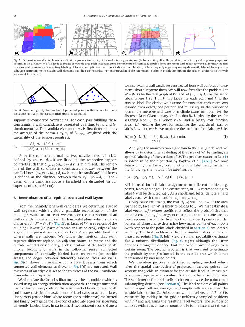
From the infinitely long wall candidates, we determine a set ofwall segments which yields a plausible reconstruction of thebuilding's walls. To this end, we consider the intersection of allwall candidate centerlines in the horizontal plane which yields aplanar graph W 0 ¼ ðV 0; E0Þ (Fig. 5(b)). Faces of W 0 are regions of thebuilding's layout (i.e. parts of rooms or outside area), edges E0 aresegments of possible walls, and vertices V 0 are possible locationswhere walls are incident. We follow the intuition that wallsseparate different regions, i.e. adjacent rooms, or rooms and theoutside world. Consequently, a classification of the faces of W 0

implies locations of walls in the following sense: connectedcomponents of identically labeled faces are rooms (or outsideareas), and edges between differently labeled faces are walls.Fig. 5(c) shows an example for a face labeling from whichconnected wall elements as shown in Fig. 5(d) are extracted. Wallthickness of an edge e is set to the thickness of the wall candidatefrom which e originates.

We formulate the face classification as a labeling problemwhich issolved using an energy minimization approach. The target functionalhas two terms: unary costs for the assignment of labels to faces of W 0

and binary costs for the assignment of label pairs to adjacent faces.Unary costs provide hints where rooms (or outside areas) are locatedand binary costs guide the selection of adequate edges for separatingdifferently labeled faces. In particular, if two adjacent rooms share a

commonwall, a wall candidate constructed fromwall surfaces of theserooms should separate them. We will now formalize the problem. LetW ¼ ðV ; EÞ be the dual graph of W 0 and let fl1;…; lk; log be the set oflabels where li; iAf1;…; kg are labels for each scan and lo is theoutside label. For clarity, we assume for now that each room wasscanned from exactly one position and thus k equals the number ofrooms; the more general case of multiple scans per room will bediscussed later. Given a unary cost function UvðlvÞ yielding the cost forassigning label lv to a vertex vAV , and a binary cost functionBv;wðlv; lwÞ yielding the cost for assigning the (unordered) pair oflabels lv; lw to v;wAV , we minimize the total cost for a labeling l, i.e.

EðlÞ ¼XvAV

UvðlvÞþX

ðv;wÞAE

Bv;wðlv; lwÞ-min: ð1Þ

Applying the minimization algorithm to the dual graphW ofW 0

allows us to determine a labeling of the faces of W 0 by finding anoptimal labeling of the vertices of W. The problem stated in Eq. (1)is solved using the algorithm by Boykov et al. [3,6,2]. We nowdefine unary and binary cost functions for label assignments. Inthe following, the notation for label vectors

Lð�Þ ¼ ðc1;…; ck; coÞ; 8 i : ci⩾0; ‖Lð�Þ‖1 ¼ 1

will be used for soft label assignments to different entities, e.g.points, faces and edges. The coefficient ci of Lð�Þ corresponding tolabel li will be denoted Lið�Þ. As a shorthand, let I i denote a hardlabel vector with ci ¼ 1, and let I ij : ¼ 1

2ðI iþI jÞ.Unary costs: Intuitively, the cost UvðlvÞ shall be low iff the area

spanned by face f in W 0 is likely to belong to lv. We first estimate alabel vector Lðf Þ whose coefficients reflect the probabilities thatthe area covered by f belongs to each room or the outside area. Anaive approach would be to project all measured points into thehorizontal plane and to determine how many points of each room(with respect to the point labels obtained in Section 4) are locatedwithin f. The first problem is that non-uniform distributions ofmeasured points (Fig. 6, left) yield a similar probability estimatelike a uniform distribution (Fig. 6, right) although the latterprovides stronger evidence that the whole face belongs to acertain room. The second problem is that we need to estimatethe probability that f is located in the outside area which is notrepresented by measured points.

We therefore propose a stratified sampling method whichtakes the spatial distribution of projected measured points intoaccount and yields an estimate for the outside label. All measuredpoints are projected into a uniform 2D grid in the horizontal plane.The side length of the grid cells is chosen as twice the point cloudsubsampling density (see Section 8). The label vectors of all pointswithin a grid cell are averaged and empty cells are assigned theoutside label vector Io. Subsequently, the label vector Lðf Þ of f isestimated by picking in the grid at uniformly sampled positionswithin f and averaging the resulting label vectors. The number ofsamples within f is chosen proportionally to the face area (at least

Fig. 5. Determination of suitable wall candidate segments. (a) Input point cloud after segmentation. (b) Intersecting all wall candidate centerlines yields a planar graph. Wedetermine an assignment of all faces to rooms or outside area such that connected components of identically labeled faces are rooms and edges between differently labeledfaces are wall elements. (c) Resulting labeling of faces after optimization; colors indicate room labels. (d) Retaining only edges separating differently labeled faces yields asubgraph representing the sought wall elements and their connectivity. (For interpretation of the references to color in this figure caption, the reader is referred to the webversion of this paper.)

Fig. 6. Considering only the number of projected points within a face for unarycosts does not take into account their spatial distribution.

S. Ochmann et al. / Computers & Graphics 54 (2016) 94–10398

one sample is enforced). The unary cost function is then defined as

UvðlvÞ : ¼ α � areaðf Þ � ‖Lðf Þ�Iv‖1; ð2Þ

where v is the vertex of W corresponding to face f in W 0, and α is aweighting factor (see Section 8). Lðf Þ is the estimated labeling offace f, and I v is the ideal expected label vector for label lv. Thedistance between these label vectors is weighted proportionally tothe area of f in order to mitigate the impact of differently sizedfaces in the sum of total labeling costs.

Binary costs: For the binary cost Bv;wðlv; lwÞ, consider edge e inW 0 to which the edge ðv;wÞ in W corresponds. Intuitively, the costfor assigning labels lv; lw to vAV and wAV shall be low iff thesurfaces of the wall represented by e are supported by measuredpoints with labels lv; lw (in the case of wall bordering the outsidearea, there should be no support on the exterior side). In otherwords, for the separation of faces with different labels lv; lw, wallelements whose surfaces are supported by points with labels lv; lwshall be preferred. For estimating the label vector for an edge e, asampling strategy similar to the face label vectors is used. Consideredge e originating from up to two wall surface lines lP1 ; lP2 (seeSection 5) with according projected support points Pxy

P1; Pxy

P2. If e

originates from a single wall surface line lP1 , we set PxyP2

¼∅.Analogous to the 2D grid in the horizontal plane, we construct aone-dimensional grid on e. The support points Pxy

P1[ Pxy

P2are

projected into the grid and their point labels are averaged percell. Empty cells are assigned the outside label. The label vectorLðeÞ is now estimated by sampling uniformly distributed points one and averaging the label vectors obtained by picking in the grid atthe sample positions. We then define the binary costs as

Bv;wðlv; lwÞ : ¼β � lenðeÞ � ð‖LðeÞ�I vw‖1þγLoðeÞÞ if lva lw;

0 otherwise;

(

ð3Þ

where v;w are the vertices of W corresponding to faces f ; g in W 0

that are separated by edge e, lenðeÞ is the Euclidean length of edgee, and β,γ are weighting factors (see Section 8) respectively. Similarto the unary costs, weighting the distance between the observedand ideal label vectors by edge length mitigates the influence ofdifferent edge lengths. The additional term LoðeÞ penalizes usageof edges with a high outside prior. We found that this term helpsto select correct edges with support points on both sides forseparating adjacent rooms. After the face labeling is determined,only edges which separate differently labeled faces are retained.The resulting subgraph W of W 0 (Fig. 5 (d)) is used in Section 7 forreconstructing connected wall elements.

Multiple scans within one room: We previously assumed thateach room was scanned from exactly one position within thatroom. In the case of more than one scan, one room is representedby a set of different labels. Fig. 7(a) shows an example of a hallwayscanned from three positions. After segmentation (Section 4), thehallway is split into multiple regions represented by differentlylabeled points (Fig. 7(b)). The graph labeling optimization sepa-rates these sections by implausible walls (Fig. 7(c)). We remove

such walls (Fig. 7(d)) as part of the opening detection in the nextsection.

7. Model generation and opening detection

From the determined graph, the final model can now bederived in a straight forward manner. The model is furtherenriched by detected window and door openings.

Walls: For each edge e ¼ ðv;wÞ of W , a wall element W isconstructed with centerline endpoints located at v and w . Thethickness of W is determined by the thickness of the wallcandidate from which e originates. Endpoints of wall elementsare connected iff the corresponding edges are incident to acommon vertex. For vertical extrusion, we first estimate floorand ceiling heights for each face f in W separately using thefollowing heuristic: consider all approximately horizontal planesdetected during wall candidate generation (Section 5). For eachplane, the number of support points located within f is deter-mined. The elevation of the plane with the largest support withinf and upwards- (resp. downwards-) facing normal is chosen as thefloor height hflðf Þ (resp. ceiling height hclðf Þ) of f . The verticalextent of a wall represented by edge f separating faces f 1; f 2 isthen defined to span the heights of both adjacent rooms:½minðhflðf 1Þ;hflðf 2ÞÞ;maxðhclðf 1Þ;hclðf 2ÞÞ�.

Opening detection: Openings in walls either arise from doorsand windows, or because a reconstructed wall was artificiallyintroduced due to multiple scans within one room as described inSection 6. By classifying detected openings accordingly, we furtherenrich the model by doors and windows, and determine whichwalls to remove for handling multiple scans within rooms. Tolocate potential openings, we determine intersection pointsbetween reconstructed walls and simulated laser rays from thescan positions to the measured points. The intersection points areclustered in the 2D domain of the wall surfaces (a simple greedy,single-linkage clustering based on distances between intersectionpoints yielded satisfactory results); see Fig. 8 (b) for an example.The clusters are then classified as doors, windows, virtual (i.e.openings due to excess walls) or invalid (i.e. clutter) by means ofsupervised learning using libsvm [5]. Six-dimensional featurevectors with the following features are used to characterizeopenings: cluster bounding box width and height, distance fromlower and upper wall bounds, approximate coverage by intersec-tion points, and a binary feature indicating whether the associatedwall is adjacent to outside area. Clusters recognized as doors orwindows are assigned to the respective wall elements. Adjacentfaces of W separated by wall elements containing at least onevirtual opening (magenta clusters in Fig. 8(b)) are merged byremoving all edges to which both faces are incident. To account forchanges after a wall removal, the determination of room heights,intersection points, clusters and opening classes is performediteratively until no more virtual openings exist.

Fig. 7. Multiple scans within a single room. (a) The hallway has been scanned from three positions; room labels are mixed within that room. (b) After segmentation(Section 4), the hallway is still split into multiple sections. (c) The labeling algorithm separates these regions by wall elements that are not part of the building's true walls.(d) By detecting and removing excess wall elements, faces are merged to larger rooms.

S. Ochmann et al. / Computers & Graphics 54 (2016) 94–103 99

8. Evaluation

We tested our approach on real-world point clouds of 14 storiesfrom 5 different buildings; statistics are given in Table 1. Theshown number of points is after subsampling with the Point CloudLibrary [14] using a resolution of ε¼ 0:02 cm (i.e. in a voxel gridwith a resolution of ε, at most one point in each voxel is retained).Normals are estimated by means of local PCA using point patchesof 48 nearest neighbors. Normals are flipped towards the respec-tive scanner position.

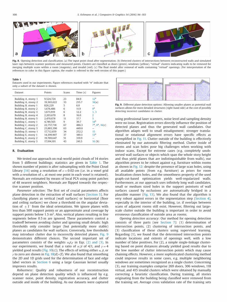
Parameter selection: The first set of crucial parameters affectsplane detection in the extraction of wall surfaces (Section 5). Forclassifying planes as vertical (wall surfaces) or horizontal (floorand ceiling surfaces) we chose a threshold on the angular devia-tion of 711 from the ideal orientations. We ignore planes withless than 500 support points or an approximate areal coverage bysupport points below 1:5 m2. Also, vertical planes resulting in linesegments below 0:5 m are ignored. These parameters control atradeoff between avoiding clutter and ignoring small details: highthresholds only consider larger (but potentially more stable)planes as candidates for wall surfaces. Conversely, low thresholdsmay introduce clutter due to incorrectly detected planes. Fig. 9demonstrates different choices. The second important set ofparameters consists of the weights α,β,γ in Eqs. (2) and (3). Inour experiments, we found that a ratio of α=β of 4/1, and γ ¼ 4yielded good results (Fig. 10(c)). The effects of setting either α, β, orγ to zero are shown in Fig. 10(d)–(f). We also found that smoothingthe 2D and 1D grids used for the determination of face and edgelabel vectors in Section 6 using a large Gaussian kernel usuallyimproves results.

Robustness: Quality and robustness of our reconstructiondepend on plane detection quality which is influenced by e.g.scanner noise, point density, registration accuracy, and clutteroutside and inside of the building. As our datasets were captured

using professional laser scanners, noise level and sampling densitywere no issue. Registration errors directly influence the position ofdetected planes and thus the generated wall candidates. Ouralgorithm adapts well to small misalignment; stronger transla-tional or rotational alignment errors have specific effects asexemplified in Fig. 11. Clutter outside of the building is effectivelyeliminated by our automatic filtering method. Clutter inside ofrooms and scan holes pose big challenges when working withindoor scans. Except for extreme cases (e.g. completely unob-served wall surfaces or objects which span the whole story heightand thus yield planes that are indistinguishable from walls), ouralgorithm proves to be robust against e.g. furniture within roomsas shown in Fig. 12: despite the presence of large scan holes, usingall available points (from e.g. furniture) as priors for roomlocalization closes holes, and the smoothness property of the usedgraph-cut-based optimization yields well-regularized walls.Furthermore, as our approach uses infinitely long wall candidates,small or medium sized holes in the support pointsets of wallsurfaces caused by occlusions are automatically bridged in aplausible manner (Fig. 13). We also found that the algorithm isvery robust against errors in the segmentation step (Section 4),especially in the interior of the building, i.e. if overlaps betweenscans of adjacent rooms still exist. However, filtering out large-scale clutter outside the building is important in order to avoiderroneous classification of outside area as rooms.

Opening detection accuracy: Our method for opening detectionconsists of three parts (see Section 7): (1) determination ofintersection points, (2) clustering of intersection points, and(3) classification of these clusters using supervised learning.Regarding (1), we found that the determined intersection pointsindicate locations and extents of openings well, with a lownumber of false positives. For (2), a simple single-linkage cluster-ing based on point distances already yielded good results due tothe low number of clutter intersection points which may causechaining effects. However, a more sophisticated clustering methodcould improve results in some cases, e.g. multiple neighboringwindows are sometimes recognized as a single cluster. Concerning(3), our training examples comprise 269 doors, 306 windows, 118virtual, and 415 invalid clusters which were obtained by manuallycorrecting a heuristic classification. During training, all storiesoriginating from the building being classified were removed fromthe training set. Average cross validation rate of the training sets

Table 1Datasets used in our experiments. Figure references marked with “n” indicate thatonly a subset of the dataset is shown.

Dataset Points Scans Time (s) Figures

Building A, storey 1 9,524,724 23 84.9 12n

Building A, storey 2 19,365,622 33 215.7 16(a)Building B, storey 1 826,229 5 6.0 —

Building B, storey 2 1,676,486 6 11.9 9n

Building B, storey 3 1,673,919 6 12.2 1, 3Building B, storey 4 2,203,670 8 16.0 2Building B, storey 5 2,470,678 11 17.7 5Building C, storey 1 4,749,565 9 39.7 14n

Building C, storey 2 22,757,718 67 486.3 7n, 8n, 16(c)Building C, storey 3 23,883,396 63 449.6 —

Building D, storey 1 17,712,659 34 252.2 15Building E, storey 1 14,399,907 37 189.3 13n

Building E, storey 2 19,769,647 51 319.9 —

Building E, storey 3 17,104,101 43 241.5 16 (b)

Fig. 8. Opening detection and classification. (a) The input point cloud after segmentation. (b) Detected clusters of intersections between reconstructed walls and simulatedlaser rays between scanner positions and measured points. Clusters are classified as doors (green), windows (yellow), “virtual” clusters indicating walls to be removed formerging multiple scans within a room (magenta), and invalid (red). (c) The final model after removal of walls containing “virtual” openings. (For interpretation of thereferences to color in this figure caption, the reader is referred to the web version of this paper.)

Fig. 9. Different plane detection options: Allowing smaller planes as potential wallsurfaces allows for more detailed structures (right-hand side) at the cost of possiblydetecting incorrect candidates in clutter.

S. Ochmann et al. / Computers & Graphics 54 (2016) 94–103100

was 90.34%, average classification accuracy was 85.02%. This smallyet significant gap indicates a generalization performance belowoptimum which we believe is caused by systematic differencesbetween e.g. the used windows in different buildings, causing thefeature vectors to not be i.i.d. Given the limited number of testdata, we think that our approach is promising, especially sincenewly obtained examples can be fed back into the algorithm.

Comparison to manually generated models: A visual comparisonbetween our reconstruction and a professional, manually gener-ated model is shown in Fig. 15. Locations and thickness of wallelements, and locations of doors are generally good; a few wallsare missing either due to the fact that (small) rooms were notscanned separately and thus room labels are missing, or becauseopenings were misclassified as “virtual” clusters.

Time and memory requirements: Our experiments were run on a6-core Intel Core i7-4930K (32 GB RAM) with a NVIDIA GeForceGTX 780 (3 GB RAM). Processing times of our prototypical imple-mentation are shown in Table 1. Peak RAM usage (incl. visualiza-tion) for the largest dataset (Fig. 16c) was about 16 GB.

Limitations: If rooms are not completely enclosed by walls(e.g. balconies or partially scanned staircases), points mighterroneously be classified as outside area during the segmentationstep which may lead to missing parts in the reconstruction. Due tothe current formulation of our approach, wall elements which arenot connected to other walls at both ends cannot be represented.

Fig. 10. Different choices for α; β; γ in Eqs. (2) and (3). (a) and (b) Perspective and orthographic view of an example situation. (c) Parameters chosen as described in Section 8.Wall centerlines are well-regularized and common wall elements have been reconstructed between rooms. (d) Without unary costs ðα : ¼ 0Þ. While the resulting walls arewell-regularized, parts of rooms are missing despite high areal support by measured points. (e) Without binary costs ðβ : ¼ 0Þ. Walls are located similar to (c) but are overlycomplex due to missing regularization and preference for correctly labeled edges. ðf Þ Without penalty for high outside labeling ðγ : ¼ 0Þ. The algorithm does not prefercommon walls for separating adjacent rooms.

Fig. 11. Effects of registration errors. (a) Result without alignment errors. Wall volumes are shown in gray together with the respective wall centerlines. (b) Translational registrationerrors may result in offset walls to which the algorithm adapts accordingly (right detail view). Wall thickness may also change (wall separating the red and green rooms in the leftdetail view). (c) Rotational registration errors may lead to wall surface pairs not to be associated to commonwalls. Wall thickness is incorrect since the wall candidates do not originatefrom wall surfaces pairs. (For interpretation of the references to color in this figure caption, the reader is referred to the web version of this paper.)

Fig. 13. Our cost minimization approach and infinitely long wall candidatesautomatically bridge scan holes in a plausible manner.

Fig. 12. Highly cluttered rooms. Left: clutter and transparent surfaces (windows)cause large scan holes; wall surfaces are only partially scanned. Right: recon-structed walls still are well regularized and separate rooms correctly.

Fig. 14. Wall elements which are not connected at both ends to other walls arecurrently not representable by our reconstruction.

S. Ochmann et al. / Computers & Graphics 54 (2016) 94–103 101

As a consequence, they are either missing (Fig. 14), or erroneouslyconnected to other wall elements. Also, since we only considerplanar wall surfaces and linear wall candidates, only piecewiselinear wall structures can be reconstructed.

9. Conclusion and future work

We presented the first automatic method for the reconstructionof high-level parametric building models from indoor point clouds.The feasibility of our approach was demonstrated on a variety ofcomplex real-world datasets which could be processed with little orno parameter adjustments. In the future, a more thorough compar-ison of reconstruction results with existing, manually generatedmodels would help to analyze reconstruction results quantitatively.A generalization to multiple building stories poses specific challengesbut would enable the reconstruction of multi-story models withoutthe need to process stories separately. Also, the usage of differentcapturing devices (e.g. mobile devices) and real-time handling ofstreamed data are topics for future investigation.

Acknowledgments

This work was partially funded by the German ResearchFoundation (DFG) under grant KL 1142/9-2 ðMoDÞ, as well as bythe European Community under FP7 grant agreements 600908(DURAARK) and 323567 (Harvest4D).

Appendix A. Supplementary material

Supplementary data associated with this article can be found inthe online version at http://dx.doi.org/10.1016/j.cag.2015.07.008.

References

[1] Adan A, Huber D. 3d reconstruction of interior wall surfaces under occlusionand clutter. In: Proceedings of international conference on 3D imaging,modeling, processing, visualization and transmission (3DIMPVT); 2011.p. 275–81.

[2] Boykov Y, Kolmogorov V. An experimental comparison of min-cut/max-flowalgorithms for energy minimization in vision. IEEE Trans Pattern Anal MachIntell 2004;26(9):1124–37.

[3] Boykov Y, Veksler O, Zabih R. Fast approximate energy minimization via graphcuts. IEEE Trans Pattern Anal Mach Intell 2001;23(11):1222–39.

[4] Budroni A, Boehm J, Automated 3d reconstruction of interiors from pointclouds. Int J Archit Comput; 2010, http://dx.doi.org/10.1260/1478-0771.8.1.55.

[5] Chang CC, Lin CJ. LIBSVM: A library for support vector machines. ACM TransIntell Syst Technol 2011;2:27(27):1–27 Software available at: http://www.csie.ntu.edu.tw/cjlin/libsvm.

[6] Kolmogorov V, Zabin R. What energy functions can be minimized via graphcuts? IEEE Trans Pattern Anal Mach Intell 2004;26(2):147–59.

[7] Monszpart A, Mellado N, Brostow G, Mitra N. RAP ter: rebuilding man-madescenes with regular arrangements of planes. In: ACM SIGGRAPH 2015; 2015.

[8] Mura C, Jaspe Villanueva A, Mattausch O, Gobbetti E, Pajarola R. Reconstruct-ing complex indoor environments with arbitrary wall orientations. In:Proceedings of EG posters; 2014.

[9] Mura C, Mattausch O, Jaspe Villanueva A, Gobbetti E, Pajarola R. Automaticroom detection and reconstruction in cluttered indoor environments withcomplex room layouts. Comput Graph 2014;44.

[10] Ochmann S, Vock R, Wessel R, Tamke M, Klein R. Automatic generation ofstructural building descriptions from 3D point cloud scans. In: GRAPP; 2014.

Fig. 16. Example results on point clouds with 33, 43, and 67 scans. Upper row: point clouds after segmentation step; most ceiling points (i.e. points with downwards-facingnormals) are removed for visualization. Lower row: reconstructed models; detected windows are shown in yellow, doors are shown in green. Most wall elements arefaithfully reconstructed; some excess walls have not been removed (see e.g. the large room in the lower-right corner of the second column). (For interpretation of thereferences to color in this figure caption, the reader is referred to the web version of this paper.)

Fig. 15. Visual comparison of reconstruction and manually generated model. (a) Input point cloud; scans are shown in different colors. (b) Professionally, manually generatedmodel. (c) Reconstructed model. Locations and thickness of walls, and locations of doors are generally good. (For interpretation of the references to color in this figurecaption, the reader is referred to the web version of this paper.)

S. Ochmann et al. / Computers & Graphics 54 (2016) 94–103102

[11] Oesau S, Lafarge F, Alliez P. Indoor scene reconstruction using primitive-drivenspace partitioning and graph-cut. In: Eurographics workshop on urban datamodelling and visualisation; 2013.

[12] Oesau S, Lafarge F, Alliez P. Indoor scene reconstruction using feature sensitiveprimitive extraction and graph-cut. ISPRS J Photogramm Remote Sens 2014;90(April (68–82)).

[13] Okorn B, Xiong X, Akinci B, Huber D, Toward automated modeling of floorplans. In: Proceedings of the symposium on 3D data processing, visualizationand transmission, vol. 2; 2010.

[14] Rusu RB, Cousins S. 3D is here: point cloud library (PCL). In: IEEE internationalconference on robotics and automation (ICRA), Shanghai, China; May 9–13,2011.

[15] Sanchez V, Zakhor A. Planar 3d modeling of building interiors from pointcloud data. In: 2012 19th IEEE international conference on image processing(ICIP); 2012. p 1777–80.

[16] Schnabel R, Wahl R, Klein R. Efficient RANSAC for point-cloud shape detection.In: Computer graphics forum, vol. 26. Wiley Online Library; 2007. p. 214–226.

[17] Tamke M, Blümel I, Ochmann S, Vock R, Wessel R. From point clouds todefinitions of architectural space. In: eCAADe 2014; September 2014.

[18] Turner E, Cheng P, Zakhor A. Fast automated scalable generation of textured3d models of indoor environments. IEEE J Sel Top Signal Process 2015;9(April(3)):409–21.

[19] Turner E, Zakhor A. Floor plan generation and room labeling of indoorenvironments from laser range data. In: GRAPP; 2014.

[20] Xiao J, Furukawa Y. Reconstructing the world's museums. In: Computer vision,ECCV 2012. Springer; 2012. p. 668–81.

[21] Xiong X, Adan A, Akinci B, Huber D. Automatic creation of semantically rich 3dbuilding models from laser scanner data. Autom Constr 2013;31:325–37.

S. Ochmann et al. / Computers & Graphics 54 (2016) 94–103 103