automatic integration of 3-d point clouds from uas and ... · automatic integration of 3-d point...

Draft

Automatic integration of 3-D point clouds from UAS and

airborne LiDAR platforms

Journal: Journal of Unmanned Vehicle Systems

Manuscript ID juvs-2016-0034.R1

Manuscript Type: Article

Date Submitted by the Author: 12-Jul-2017

Complete List of Authors: Persad, Ravi; York University Armenakis, Costas; York University, Department of Earth and Space Science and Engineering; Hopkinson, Chris; University of Lethbridge Brisco, Brian; Natural Resources Canada Earth Sciences

Keyword: point clouds, UAS, LiDAR, matching, registration, automation

Is the invited manuscript for consideration in a Special

Issue? : UAV-g (Unmanned Aerial Vehicles in geomatics)

https://mc06.manuscriptcentral.com/juvs-pubs

Journal of Unmanned Vehicle Systems

Draft

1

Automatic registration of 3-D point clouds from

UAS and airborne LiDAR platforms

Ravi Ancil Persad1, Costas Armenakis

1, Chris Hopkinson

2, Brian Brisco

3

1York University,

2University of Lethbridge,

3Natural Resources Canada

Abstract: An approach to automatically co-register 3-D point cloud surfaces from

Unmanned Aerial Systems (UASs) and Light Detection and Ranging (LiDAR)

systems is presented. A 3-D point cloud co-registration method is proposed to

automatically compute all transformation parameters without the need for initial,

approximate values. The approach uses a pair of point cloud height map images for

automated feature point correspondence. Initially, keypoints are extracted on the

height map images, and then a log-polar descriptor is used as an attribute for matching

the keypoints via a Euclidean distance similarity measure. Our study area is the

Peace-Athabasca Delta (PAD) situated in north-eastern Alberta, Canada. The PAD is

a world heritage site, therefore regular monitoring of this wetland is important. Our

method automatically co-registers UAS point clouds with airborne LiDAR data

collected over the PAD. Together with UAS data acquisition, our approach can

potentially be used in the future to facilitate automated co-registration of

heterogeneous data throughout the PAD region. Reported transformation parameter

accuracies are: a scale error of 0.02, an average rotation error of 0.123° and an

average translation error of 0.237m.

Keywords: point clouds, UAS, LiDAR, matching, registration, automation

Page 1 of 38



Draft

2

Introduction

In the geomatics engineering community, Unmanned Aerial Systems (UASs) have

received considerable attention and continue to be an area of significant interest for

both academia and industry. As we move forward, UAS technology will continue to

strongly influence future commercial trends and research directions undertaken in

various geospatial fields such as urban planning, cadastral and topographic

surveying/mapping, photogrammetry and low-altitude remote sensing. However,

significant advancements may not always necessarily come from a single technology

but through the integration of multiple technologies and their respective data.

UAS platforms provide many benefits including portability and cost-effective data

acquisition. UASs can potentially have a substantial impact due to their capability and

convenience for flying on a frequent basis. UASs also have low mobilization and

operational costs, thus facilitating continuous data acquisition for mapping

applications. This is critical for various applications such as topographic mapping /

map-updating of smaller areas and for detecting changes in non-urban (e.g., glaciers,

icefields, rivers) and urban (e.g., cities) environments. Nevertheless, there are also

several limitations with geospatial data collected by UASs. Coverage of an area may

be hindered due to short flight times and payload restrictions of the UAS. This may be

sufficient for ‘small-scale’ mapping of an area but will not suffice for larger projects

with time restrictions. Quality and accuracy of data is another concern with UAS-

generated data. Small, non-metric cameras are often utilized for UASs. However, the

majority of these cameras have low-resolution and are prone to various types of lens

distortions. As a result, the density and accuracy of 3-D point clouds generated via

Page 2 of 38



Draft

3

structure-from-motion (SFM) algorithms (Forsyth and Ponce 2002) will be negatively

affected. In such instances when there are coverage and accuracy concerns for data

collection, combinations of sensors and platforms such as airborne Light Detection

and Ranging (LiDAR) systems, satellites and large airborne metric camera systems

are instead employed. These sensors are considerably more expensive and complex

when compared to small UASs. Therefore, data acquisition from these larger

platforms has higher operational and processing costs. Data integration requires that

all datasets must be referenced in the same coordinate system. Generally, data co-

registration is achieved by the manual selection of corresponding feature points on the

source and target datasets to be aligned. Multi-sensor data integration is commonly

referred to as alignment or co-registration in the fields of photogrammetry and

computer vision. Due to the large amounts of point data collected and the repeated

periods of data acquisition as with the case for map revision, automatic co-registration

is desired. This minimizes or eradicates the need for manual input from a human

operator.

The data co-registration problem

The objective of co-registration is to align a source dataset with a target dataset.

The source and target datasets are typically in different coordinate systems which vary

in terms of a scale factor, rotation angles and translational shifts. Automatic co-

registration of a dataset pair (i.e., a source dataset and a target dataset) is a two-fold

problem. The first aspect is the ‘correspondence’ problem. This refers to the

extraction and establishment of conjugate geometric key features (e.g., points, lines or

planes) on both the source and target domains by matching their feature attributes.

Page 3 of 38



Draft

4

The second issue is the ‘transformation’ problem and refers to the computation of

transformation parameters using the corresponding key features. The determination of

the relationship between two 3-D coordinate systems is a well-studied area and has

various applications in both photogrammetry and computer vision (Lorusso et al.

1995). It has been referred to as the 3-D similarity (or conformal) transformation or

the absolute orientation problem over the years. Nevertheless, the objective remains

the same, i.e., the estimation of rotational, translational and scalar elements which are

required to bring a pair of 3-D objects from two different Cartesian coordinate

systems into a common system, thereby aligning them. In our case, we seek to

transform the source point clouds, �� into the system of the target point clouds,

�� using Eq. (1).

�� = �� + ��1�

where, � is the single, global scaling factor,

� is a 3x3 orthogonal rotation matrix comprising three angles, ω, φ, κ,

� is a 3x1 translation vector with 3 components, (tx, ty, tz),

��

is the �� when aligned with ��.

Related work on UAS and LiDAR point cloud integration

There has been prior work in the area of point cloud integration from UAS and

LiDAR sensors. Generally, UAS point clouds are generated in an un-georeferenced

local photo coordinate system via SFM, whilst LiDAR point data is typically derived

in a georeferenced coordinate system. In this case, UAS data can be georeferenced

using ‘direct’ or ‘indirect’ georeferencing approaches (Colomina and Molina 2014).

Page 4 of 38



Draft

5

In the latter, surveyed ground control points are used to estimate the position and

orientation of the sensor platform through photogrammetric triangulation, while the

former case directly uses position and orientation parameters provided by navigation

sensors from the global navigation satellite systems (GNSS) and inertial measurement

units (IMUs).

A case of the direct georeferencing approach to co-register UAS data with 3-D

LiDAR point clouds has been presented by Yang and Chen (2015). They collected

images and LiDAR points using a rotor-type mini-UAS equipped with a Canon 5D

Mark II camera and Riegl LMS-Q160 scanner. Position and orientation of the UAS

are computed using an on-board Novatel Span GNSS/IMU receiver through direct

georeferencing. These position and orientation transformation parameters were used

for alignment of the LiDAR point cloud data to the UAS images. Afterwards, dense 3-

D points were computed using the UAS imagery. While the two datasets are now in

the same reference system, an additional step was necessary to refine the UAS to

LiDAR point cloud co-registration. The well-known Iterative Closest Point (ICP)

algorithm (Besl and McKay 1992) was used for this purpose. Their approach relies on

data collected from the GNSS and the IMU sensors. GNSS positioning may be

affected due to satellite geometry and availability, as well as other systematic effects

such as multi-path, while IMU data are known to degrade over time.

Therefore, we seek a purely data-driven co-registration approach such as those

presented in Novak and Schindler (2013), and in Persad and Armenakis (2015). Their

methods utilized automatic feature extraction and feature correspondence to co-

Page 5 of 38



Draft

6

register 3-D point clouds from UAS and LiDAR systems. Both works relied on the

projection of the 3-D point clouds into a 2-D planimetric height map image domain to

perform the matching process.

Persad and Armenakis (2015) automatically extracted 2-D height map image point

features or ‘keypoints’ on both the UAS and LiDAR datasets using a surface

curvature-based keypoint detector. Afterwards, they formed attributes or descriptors

of these 2-D keypoints. Specifically, they utilized the ‘SURF’ keypoint descriptor

(Bay et al. 2008) for the matching process. The SURF descriptor is based on the

computation of Haar wavelet filter statistics in both the horizontal and vertical image

directions. Keypoints with similar descriptors from both UAS and LiDAR datasets are

then established as corresponding points. The associated 3-D coordinates of matched

2-D keypoints are then used for computing the 3-D conformal transformation

parameters to enable the co-registration of UAS and LiDAR point clouds. On the

other hand, Novak and Schindler (2013) employed local image gradient information

as a feature descriptor. The hypothesized and test algorithm, RANdom SAmple

Consensus (RANSAC) (Fischler and Bolles 1981) was then used to find matching

point features.

Automatic alignment of UAS and LiDAR point clouds

In this work, we address the alignment of 3-D point cloud datasets generated by

SFM from overlapping UAS camera images with those obtained by airborne LiDAR.

Therefore, our objective is the computation of the seven-parameter 3-D conformal

transformation (i.e., scale factor s, three rotation angles (ω, φ, κ), three translations

Page 6 of 38



Draft

7

(tx, ty, tz)) using automatically determined corresponding keypoints. Fig. 1 depicts

the general procedure for 3-D co-registration using UAS and LiDAR point clouds.

We assume that the input UAS and LiDAR point clouds to be co-registered are in

different coordinate reference systems and have different scales, point densities, point

distributions, and accuracies. The UAS point clouds are treated as the ‘source’ data

which has to be co-registered with the ‘target’ LiDAR point clouds. Their respective

2-D height map raster surfaces (i.e., height map images) are used for the feature

matching method. In this work, we propose a keypoint feature matching framework

for point cloud co-registration. Similar to the reviewed literature, height map images

are used to find matching features. However, compared to the previous works, we use

a different keypoint detector and keypoint descriptor. In particular, we utilize a multi-

scale, 2-D keypoint detector and a log-polar based scale, rotation and translation

invariant point descriptor to find matching keypoints.

Keypoint extraction on height map images

In computer vision tasks, the objective is to design and build automated algorithms

which are capable of replicating the capabilities of biological vision (i.e., the human

visual system). As highlighted in Medathati et al. (2016), concepts in biological vision

(e.g., detection and recognition of objects, pattern grouping and classification, scale-

space approaches, and motion estimation) are used as a source of inspiration when

designing computer vision algorithms and frameworks. Steerable pyramids

(Simoncelli and Freeman 1995) facilitate multi-scale image representation and

comprise of multi-oriented (i.e., steerable) Gaussian derivative filters computed at

Page 7 of 38



Draft

8

multiple levels (i.e., different image scales).

Our spatial point cloud data has been projected to height map images. We employ a

multi-scale approach to detect keypoints on both the UAS and LiDAR height map

images. Multi-scale image analysis is particularly useful for simulating the scale-

space representation of real world objects as typically perceived by human vision.

That is, as we physically move away from an object, the finer details are lost whilst

‘stronger’ and more prominent features remain visible. Utilization of scale-space is

beneficial for localizing distinct keypoints on prominent real-world structures as we

move from high to low down-sampled, resolution versions of the same image. As

discussed in Lindeberg (2013), there are two main reasons for employing multiple

scales in computer vision and image processing problems: i) the first is to provide a

multi-scale representation of the real-world data, and ii) to suppress and eliminate

unnecessary details in an effort to retain only the most salient and distinct features of

interest.

In this work instead of regular Gaussian filters, we use complex-steerable pyramids

proposed by Portilla and Simoncelli (2000) as they are based on complex filters which

mimic characteristics of biological vision. They differ from regular steerable

pyramids since they utilize real and imaginary symmetric derivative filters to produce

complex-valued image sub-bands. An input image is first subjected to a low-pass

filter. The low-pass image band is then split into � lower sub-band images ′��′using

complex filters of different orientations. A pyramidal structure is formed through

recursive down-sampling of the low pass image by a factor of 2 and once again multi-

directional complex filters are applied. This is done for � specified levels. We

empirically set � = 10 to obtain sufficient directional coverage every 36°, and � = 5

Page 8 of 38



Draft

9

to provide sufficient level of details to detect salient key features.

!"#$%&'�'(!&)'ℎ+ = min/��{1,….,5}/�2�

Using the � complex-valued ��coefficients, we compute a keypoint ‘strength’

map at each level�. This is done using the keypoint strength function in Eq. (2). A

similar function has been employed by Bendale et al. (2010) and is related to the

keypoint criteria also used by the popular Förstner interest point operator (Förstner,

1994). After keypoints are obtained at all � levels, we transfer them to the original

height map image space. Repeated keypoints which are detected at the same positions

on more than one level apart are filtered, i.e., the keypoint with the highest strength is

retained. In the next step, we assign descriptors (or attributes) to these keypoints.

Assigning descriptors to extracted keypoints

Our UAS and LIDAR height map images are in different coordinate systems and

differ in terms of scale, rotation and translation. This greatly increases the complexity

of finding corresponding keypoints that were extracted on both the UAS and LIDAR

height map images. To address this, we use a keypoint descriptor which is invariant to

scale, rotation and translation differences between the pair of height map images.

Specifically, we adopt a log-polar based descriptor estimated from the local image

neighborhood around each keypoint (Kokkinos et al. 2012).

A log-polar grid system was used to sample the neighbourhood of the keypoint to

determine descriptors characterizing the keypoint based on local height changes. The

Page 9 of 38



Draft

10

log-polar grid system can represent the image information (height map) with a space-

variant resolution inspired by the visual system of mammals (Traver and Bernadino

2010). The log-polar gridding and mapping causes any rotation and scale differences

between the images to be manifested as a translational, cyclical shift in the log-polar

descriptor space. The Fast Fourier Transform is then applied to correct this shift and

produce the final transformation-invariant descriptor to be used for determining

keypoint correspondences. We briefly describe the two main steps used to compute

the keypoint descriptor as follows:

i) Log-polar grid sampling and mapping: First, a log-polar grid centered on a

keypoint is generated. The grid is made up of a number of concentric rings with

exponentially increasing radii, as well as, a number of equally-spaced rays projecting

radially from the keypoint to the boundary of the outermost concentric ring, thus

forming sectors on the grid. The radius for the innermost and outer ring is empirically

set at 3 and 50 pixels respectively. We also experimentally define the number of

concentric rings as 8 = 25and the number of rays as 9 = 30 to obtain sufficient

descriptor details for the matching process. Grid sampling points are formed when the

rays intersect the concentric rings. Afterwards, 8 directional image derivatives are

computed at each log-polar grid sample point. Derivatives are used because they are

invariant to intensity changes on images and provide structural attributes for feature

matching. As the radii increases, the derivatives are smoothed using a Gaussian kernel

with an increasing scale to avoid image aliasing due to the non-uniform log-polar

sampling pattern (Tabernero et al. 1999). The derivatives are then mapped to a

uniformly spaced log-polar image domain. By transferring to the log-polar space, any

Page 10 of 38



Draft

11

rotation and scale changes between true keypoint correspondences on the source and

target height map images will now be represented as a translational cyclic shift.

ii) Shift-invariance using the 2-D Fast Fourier Transform (FFT): At this point,

potentially corresponding source and target keypoint descriptors will not match since

their respective log-polar descriptors differ by a cyclical shift. Therefore, we apply a

2-D Fast Fourier Transform (FFT) (Cooley and Tukey 1965) on the feature space of

the log-polar descriptors which produces a shift-invariant descriptor representation.

Finding matching keypoint descriptors

A combination of nearest neighbour distance ratio (��;�) (Lowe 2004) and

RANSAC is used for establishing corresponding keypoints. ��;� is firstly applied

to find initial, candidate keypoint matches, followed by RANSAC to prune

wrong/outlying correspondences. ��;� is based on using the Euclidean distances

between source and target keypoint descriptor vectors in the descriptor feature space.

For a source keypoint descriptor, the Euclidean distance (<;) metric is used to find

the target descriptor which is its nearest neighbour. This distance is recorded (<;1).

We also store the target descriptor which is the second closest neighbour. This

distance is also recorded (<;=). Efficient nearest neighbour searching is achieved

using k-d trees (Bentley 1975). ��;� is the ratio of the distances between the first

and second nearest neighbours (Eq. (3)). If ��;� is less than a threshold τ, a source

to target keypoint match is accepted (we empirically set τ = 0.3).

Page 11 of 38



Draft

12

��;� =<;1<;=

�3�

After ��;� matching, the RANSAC algorithm (Fischler and Bolles 1981) is

applied to filter wrong matches which may have been retained. We note here that the

height map image keypoints also have an accompanying elevation coordinate (i.e., a

‘Z’ component). The input for RANSAC are the 3-D positions of the keypoints (i.e.,

X, Y and Z values), since our aim is to estimate the best 3-D conformal

transformation for optimum 3-D data alignment. RANSAC begins by randomly

sampling the three minimum number of keypoint matches required to estimate the 3-

D conformal transformation parameters. These candidate parameters are estimated

using the linear least squares method originally developed by Horn (1987). To test if

this candidate transformation is optimal, we use its seven parameters to project the

source keypoints to the target point cloud domain. Inlying matches are stored if a

source keypoint is less than a value of 0.5m to a target keypoint. The total number of

inliers is stored and the iterative RANSAC loop repeats. After the iterations are

complete, the candidate transformation which gives the highest inlier count is chosen

as the optimal estimation of the point cloud co-registration parameters. A final 3-D

conformal transformation is then computed using all inlying keypoint matches via

least squares adjustment (Wells and Krakiwsky 1971). This provides the most

suitable scale factor, 3-D rotation and 3-D translation which align the UAS and

LiDAR point clouds.

Page 12 of 38



Draft

13

Study Area

Our study area is the Peace-Athabasca Delta (PAD) (area: 794,000 acres) situated

in north-eastern Alberta, Canada (latitude: 58° 42’N, longitude: 111° 30’W).

Following the retreat of the Laurentide ice sheet (approximately 10,000 BP (Before

Present)), the PAD was formed in the western region of Lake Athabasca. Deltas were

formed by the three major rivers (Peace, Athabasca and Birch rivers) (PADPG 1973).

Over 1,000 lakes and wetland basins have been formed across this inland delta

(Jaques 1989).The PAD is located in the Wood Buffalo National Park, which is a

designated UNESCO heritage site and its conservation is of utmost importance.

Therefore, there is significant value in developing an approach to automatically

integrate multi-sensor and multi-temporal datasets, which can then be applied for

future uses such as the continuous and frequent monitoring of the PAD wetland

region. We will be using UAS and airborne LiDAR 3-D point clouds to assess our

proposed co-registration method.

Data collection

Unmanned aerial system

The UAS used in this work was a DJI Phantom 2 Vision+ (Fig. 2). Weighing 1.2

kgs and approximately 29 cm in width, the UAS has a maximum flying speed of 53.9

km/h. The system has four propellers which stabilizes motion and has an onboard

gyroscope, accelerometer and GNSS receiver. The UAS can be remotely controlled or

be flown according to pre-programmed flight plans. A ground station software was

used for image/video feed to facilitate real-time navigation. An onboard video

transmitter sends camera data to the ground control station. A 14 megapixel camera

Page 13 of 38



Draft

14

attached to the UAS was used to collect image data of the PAD region. The camera

uses a three-axis gimbal for pivoted rotation support. Images can be captured at pre-

set, regular intervals or via manual triggers.

UAS and airborne LiDAR datasets

A UAS fieldwork survey campaign was undertaken from August 9-17, 2015 (Li-

Chee-Ming et al. 2015). Both manual flights and pre-planned flights were carried out.

Manual flights were conducted with coverages of up to 120m×500m, whilst those

based on pre-planned grids had flight coverages of 200m×200m. Manually

controlled flights were predominantly conducted in order to capture images with more

heterogeneous characteristics of the study site, including mud flats, vegetated regions

and water surfaces. This is critical for SFM post-processing, since overly

homogeneous imagery with low contrast and repeated textural patterns can pose

problems when trying to automatically match image features.

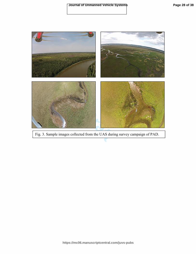
For UAS data collection during manual flights, the camera was set to capture

images at 20 m distance intervals. This facilitated an 80% forward image overlap and

a 40% side image overlap with flying heights ranging from 80 m to 90 m. Both nadir-

looking, vertical images, in addition to oblique images of the area were captured.

These high resolution images had dimensions of 4608 x 3456 (i.e., height × width).

Fig. 3 shows various sample UAS imagery. To generate dense 3-D point clouds from

the images, the Agisoft Photoscan software (Agisoft 2016) was employed. Agisoft

uses SFM to generate the 3-D point cloud model from the UAS imagery (Fig. 4).

Page 14 of 38



Draft

15

The airborne LiDAR terrain data for the PAD region was collected on July 28,

2015 using an Optech Aquarius airborne topo-bathymetric LiDAR system. The

airborne system operated at 532 nm and flew approximately 800 m above ground

level. The Aquarius operates in the visible portion of the spectrum and is not eye-safe.

To reduce the energy concentration within the footprint the pulses were spaced more

in time and the beam was widened (Hopkinson et al. 2016). Optech LiDAR Mapping

Suite was used to process/calibrate the raw point data collected during the airborne

LiDAR survey. Bentley Microstation with the Terrasolid Terrascan application was

used for point cloud data cleaning. The generated UAS point clouds were computed in

the local photo coordinate system. The LiDAR point clouds were georeferenced in the

Universal Transverse Mercator (UTM) North American Datum of 1983 (NAD83),

Zone 12. Both sets of point clouds were non-uniformly distributed and had different

point densities. Fig. 5 (a) shows the UAS point clouds and Fig. 5 (b) are the LiDAR

point clouds.

To assess our co-registration method, we selected a prominent mud lake in the

study area appearing in both datasets (Fig. 5). We manually delineate the mud lake

point clouds on the LiDAR dataset using a 3-D polyline (shown as a red curved

polyline in Fig. 5 (b)). The UAS and LiDAR point cloud datasets were interpolated to

2-D raster elevation height maps of 1 by 1 pixel and 1 by 1 meter cells respectively

using the natural neighbour algorithm (Childs 2004). Since the LiDAR points consist

of multiple returns, the generated LiDAR surface is not exactly equivalent to that of

the UAS surface at vegetated regions as they may contain ground points.

Page 15 of 38



Draft

16

Results and analysis

The co-registration is assessed in two ways. First, we compare the parameters

computed using the proposed, automatic method with those derived from point

correspondences manually collected by a human operator. Secondly, we analyse the

differences between the automatically aligned UAS and LiDAR 3-D point surfaces.

In this case, co-registration results are validated by analysing the elevation

differences between the two aligned datasets as a result of: i) errors incurred during

the alignment process, ii) errors in the data, and iii) possible temporal changes.

Accuracy of proposed automated co-registration

In this section, we present the results of the estimated 3-D conformal

transformation parameters (i.e., scale factor s, three rotation angles (ω, φ, κ), three

translations (tx, ty, tz)) which have been derived using our proposed automated

method relative to their reference transformation parameters. The reference

parameters are essentially, our “ground truth” values, were determined by manually

selecting 15 matching keypoints on the UAS and LiDAR point clouds. Using our

approach, 18 keypoints were automatically extracted on the UAS height map image,

and 33 keypoints were detected on the LiDAR height map image. There were a total

of 14 point matches and 3 outliers, which were eliminated via RANSAC. Therefore,

11 inlying keypoint correspondences were established and used to compute the

automated transformation parameters. Fig. 6 shows our automatic keypoint matches

between the UAS and LiDAR height map images. The point distribution shows a

linear pattern due to the UAS data which was collected around water bodies in order

to determine the land-water boundaries.

Page 16 of 38



Draft

17

Figs. 7 and 8 illustrate the 3-D keypoint correspondence residuals after least

squares adjustment has been applied to derive the reference and automated

transformation parameters respectively. The residuals indicate how well the source

keypoints fit to their corresponding target keypoints, following the least squares

minimization process. On observing the plots in Figs. 7 and 8, both the manually

selected and automatically-derived keypoint correspondences had residuals with sub-

meter level accuracy.

From the least squares adjustment process, we also use two metrics for assessing

co-registration accuracy, namely the precision of the estimated transformation

parameters (?@� �� and ?A��B��), as well as the root mean square error of

keypoint observation X, Y and Z residuals (RMSEResiduals). These are shown in Table

1. Also reported are the errors in scale, rotation angles and translations with respect

to the reference parameters, i.e. absolute scale error |��|, absolute mean rotation

error (AMRE) and absolute mean translation error (AMTE). We note that: i) when

computing the co-registration parameters, the UAS point clouds are set as the source

dataset and the LiDAR point clouds are set as the target dataset, and ii) the NAD83

‘X’ and ‘Y’ coordinate values of the LiDAR point clouds are large values, therefore

to prevent numerical instabilities while applying least squares adjustment, we shifted

the data into a local centroid system resulting in smaller values of the coordinates.

Based on Table 2, when compared to the reference “ground truth” we obtained a

scale error of 0.02, rotation error of 0.123° and translation error of 0.237m. To further

reduce the alignment errors we use the Iterative Closest Point (ICP) algorithm (Besl

and McKay 1992) as an additional refinement of the co-registration. The ICP uses the

Page 17 of 38



Draft

18

entire set of source and target point clouds for correspondences as opposed to sparse

keypoint matching. ICP forms corresponding point pairs based simply on the closest

point criteria in the 3-D Euclidean space. Then, the sum of squared distances between

all these pairs is iteratively minimized and refined 3-D conformal transformations are

continually estimated using Horn’s method (Horn 1987). This iterative loop stops

when the mean distance error of all corresponding points is less than a set threshold or

when the difference between consecutive mean distance errors is smaller than a

certain value. We use the latter criteria and a value of 1e-05m is empirically set to

determine when the error change is minimal.

The RMSE of source keypoint positions relative to the target keypoints reduced

from 0.468m (i.e., based on initial co-registration) to a value of 0.351m, indicating

closer alignment. Fig. 9 shows the co-registration result of the 3-D point clouds from

the UAS and LiDAR based on the automated keypoint matching and ICP refinement,

including data points beyond the range of location of keypoints. Based on Fig. 9 (b),

we can see in the extrapolated region of the dataset (right side of zoomed-in window)

that the delineated LiDAR mud lake point cloud polyline (in red) has a closer

alignment with the RGB, textured UAS point clouds after the ICP is applied.

Analysis of the co-registration between the UAS and LiDAR datasets

Due to the close temporal proximity of data acquisition, let us assume that the

UAS and LiDAR point clouds differ by a 3-D conformal transformation and no

deformations (e.g., data errors, possible temporal variations) are present. After the

co-registration, we expect that the two point cloud surfaces overlap and match each

Page 18 of 38



Draft

19

other, such that the spatial difference of the two surfaces should be zero. This would

be the ideal result. However, we anticipate there will be some discrepancies due to

several factors including: i) errors in the automated co-registration process, ii)

possible temporal differences between the two surfaces, iii) difference in data types

(for e.g., vegetation canopy versus ground points as the UAS point cloud surface

model captures the surface of tree/vegetated regions, whilst the LiDAR data include

ground points due to LiDAR signal penetration in vegetation/tree canopy regions),

and iv) errors in the coordinates of both datasets (e.g., system calibration errors,

image matching errors).

To validate the co-registration of the UAS and LiDAR data, we estimate and

analyse the differences between their respective height map raster surfaces. Since we

have no available field validation data of detected differences, based on the

conformal assumption between the two datasets, we apply a normalization of the two

datasets to minimize any bias effect of possible UAS and LiDAR elevation

differences (Eq. (4)).

Normalized@�� =�L�'!( − N!L&@��

�'L&OL(OO!P%L'%$&@��4�

We also compute elevation differences that are within standard deviation confidence

intervals. Specifically, we generate and assess differences at a 68% confidence

interval (± 1σ), 95% confidence interval (± 2σ) and at 99% confidence interval (±

Page 19 of 38



Draft

20

3σ), where σ is the standard deviation of elevation differences between the UAS and

LiDAR height maps.

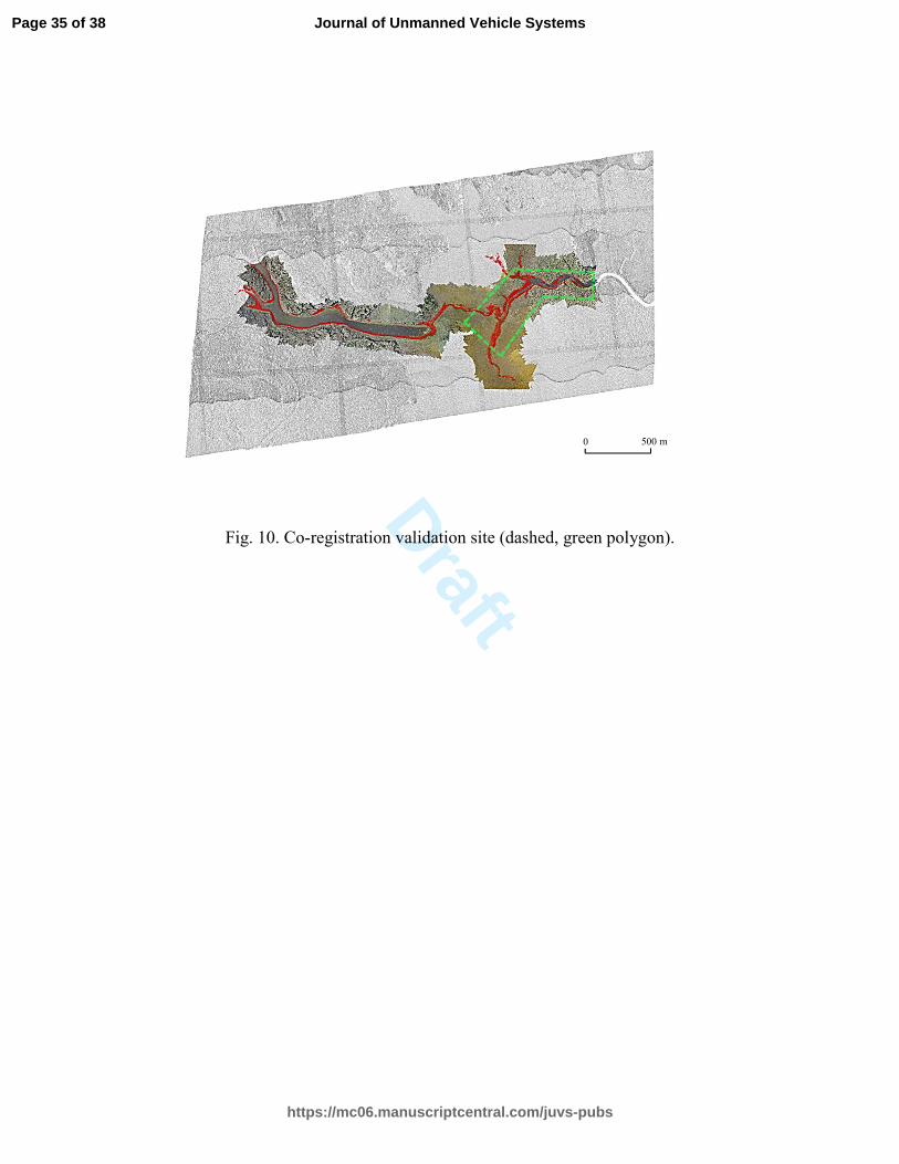
We selected a sub-region of the dataset for assessing the co-registration

discrepancies between the two datasets (Fig. 10). Fig. 11 illustrates the normalized

height maps. After the normalized UAS and normalized LiDAR height maps are

generated, we compute the height differences of both raster surfaces to determine

possible elevation mismatches. Based on the statistical σ ranges, elevation differences

inside the 68%, 95% and 99% tolerance bounds are shown as areas of ‘no differences’

on the mis-matching maps of Fig. 12. The elevation differences lying outside the ±1σ,

±2σ or the ±3σ bounds are then considered to be the significant differences between

the two datasets. These are shown as the areas of ‘detected differences’ in Fig. 12. On

observing these detected difference regions, we notice that at the ± 1σ level, there are

elevation differences around the perimeter of the mud lake. As we increase the

tolerance levels to ± 2σ and ± 3σ, the majority of elevation differences occur in

homogeneous vegetated areas. We associate these differences with: i) feature

matching blunders incurred during the UAS’s SFM point cloud generation process,

which introduce errors into the generated 3-D coordinates, and ii) due to the fact that

the generated LiDAR surface represents a sort of mid-canopy elevation model in areas

with tree and shrub coverage due to the possible existence of ground points, where

height differences between vegetation and ground surfaces could be up to several

Page 20 of 38



Draft

21

Conclusions

The objective of this study was to develop and test an approach to automatically

align UAS and LiDAR point clouds collected for the PAD region in Alberta, Canada.

The purpose of automated point cloud alignment is to aid in the continuous

monitoring of the PAD wetland area on a frequent basis using data collected from

multiple sensors or multiple data acquisition platforms. The UASs provide an

effective means of rapid and efficient data acquisition which is ideal for wetland

mapping, monitoring and validation applications.

Manual co-registration of multi-sensor data is time-consuming and depending on

the coverage of the study area can also be labour intensive. Our proposed method

overcomes these limitations by automatically detecting ‘virtual’ ground control points

referred to as keypoints. The keypoint extraction method is based on multi-scale

image analysis applied to the point cloud height maps. Source and target point clouds

differ by scale, rotation and translation; therefore we developed a scale, rotation and

translation invariant attribute or descriptor which is assigned to the keypoints. These

descriptors are used to find corresponding keypoints by checking the similarity of

their Euclidean distances. Our matching approach is also able to co-register point

cloud datasets which have different point distributions (e.g., uniform or non-uniform)

and different point densities.

The results presented are preliminary and based on a small dataset sample. Our co-

registration approach needs to be further validated with more datasets. In addition, the

PAD area comprises monotonous patterns of wetlands, bare mud-land and upland

Page 21 of 38



Draft

22

forest cover. This lack of heterogeneity provides challenges in identifying and

matching distinct keypoints. Therefore, we also plan to explore alternative means of

automatic matching which can utilize other types of features such as curvilinear ones,

which are prominent along rivers and lakes throughout the delta.

Acknowledgements

This study has been financially supported by the Natural Sciences and Engineering

Research Council of Canada (NSERC), Kepler Space Inc., and the Government of

Canada, specifically through the Canadian Space Agency (CSA) Government Related

Initiative Program (GRIP) and through Natural Resources Canada / Canada Centre for

Mapping and Earth Observation (NRCan / CCMEO). Additional funding to support

the associated airborne and lab costs from the University of Lethbridge has been

provided by Campus Alberta Innovates Program, NSERC Discovery, and Alberta

Innovation and Advanced Education. We wish to express our sincere thanks to Julien

Li-Chee Ming, Dennis Sherman and Keith Menezes of York University for collecting

and processing the UAS data, Kevin Murnaghan of NRCan / CCMEO for providing

the GPS coordinates for the georeferencing of the UAS data, and Joshua Montgomery

of the University of Lethbridge for processing the LiDAR dataset.

References

Agisoft, 2016. http://www.agisoft.com/ (Accessed 21.5.2016).

Bay, H., Ess, A., Tuytelaars, T., and Van Gool, L. 2008. Speeded-up robust features

(SURF). Computer vision and image understanding 110, no 3: 346-359.

Bendale, P., Triggs, W., and Kingsbury, N. 2010. Multiscale keypoint analysis based

on complex wavelets. In BMVC 2010-British Machine Vision Conference (pp. 49-1).

BMVA Press.

Page 22 of 38



Draft

23

Bentley, J.L. 1975. Multidimensional binary search trees used for associative

searching. Communications of the ACM, 18(9), pp.509-517.

Besl, P.J., and McKay, N.D. 1992. Method for registration of 3-D shapes.

In Robotics-DL tentative (pp. 586-606). International Society for Optics and

Photonics.

Childs, C. 2004. Interpolating surfaces in ArcGIS spatial analyst. ArcUser, July-

September, 3235.

Cooley, J.W., and Tukey, O.W. 1965. "An Algorithm for the Machine Calculation of

Complex Fourier Series." Math. Comput. 19, 297-301.

Colomina, I., and Molina. P. 2014. Unmanned aerial systems for photogrammetry and remote sensing: A review. ISPRS Journal of Photogrammetry and Remote Sensing, 92, pp.79-97.

Förstner, W. 1994. May. A framework for low level feature extraction. In European

Conference on Computer Vision (pp. 383-394). Springer Berlin Heidelberg.

Forsyth, D.A. and Ponce, J. 2002. Computer vision: a modern approach. Prentice

Hall Professional Technical Reference.

Hopkinson, C., Chasmer, L., Gynan, C., Mahoney, C. and Sitar, M. 2016. Multi-

sensor and Multi-spectral LiDAR Characterization and Classification of a Forest

Environment. Canadian Journal of Remote Sensing, Vol. 42 , Iss. 5, 501-520.

Horn, B.K. 1987. Closed-form solution of absolute orientation using unit

quaternions. JOSA A, 4(4), 629-642.

Jaques, D.R. 1989. Topographic Mapping and Drying Trends in the Peace-Athabasca

Delta, Alberta Using LANDSAT MSS Imagery. Report prepared by Ecostat

Geobotanical Surveys Inc. for Wood Buffalo National Park, Fort Smith, Northwest

Territories, Canada, 36 pp. and appendix.

Kokkinos, I., Bronstein, M.M., and Yuille, A. 2012. “Dense scale invariant

descriptors for images and surface,” Technical Report, INRIA.

Li-Chee-Ming, J., Murnaghan, K., Sherman, D., Poncos, V., Brisco, B., and

Armenakis, C., 2015. Validation of Spaceborne Radar Surface Water Mapping with

Optical sUAS Images. The International Archives of Photogrammetry, Remote

Sensing and Spatial Information Sciences, 40(1), p.363.

Lindeberg, T. 2013. Scale-space theory in computer vision (Vol. 256). Springer

Science & Business Media.

Lorusso, A., Eggert, D., and Fisher, R. 1995. A Comparison of Four Algorithms for

Page 23 of 38



Draft

24

Estimating 3-D Rigid Transformations. In Proceedings of the 4th British Machine

Vision Conference BMVC ’95, pages 237–246, Birmingham, England.

Lowe, D.G. 2004 Distinctive image features from scale-invariant keypoints.

International journal of computer vision 60, no 2: 91-110.

Medathati, N.K., Neumann, H., Masson, G.S., and Kornprobst, P. 2016. Bio-inspired

computer vision: Towards a synergistic approach of artificial and biological

vision. Computer Vision and Image Understanding, 150, pp.1-30.

Novak, D., and Schindler, K. 2013. Approximate registration of point clouds with

large scale differences. ISPRS Annals of Photogrammetry, Remote Sensing and

Spatial Information Sciences, 1(2), pp.211-216.

Peace-Athabasca Delta Project Group (PADPG). 1973. Peace-Athabasca Delta

Project, Technical Report and Appendices, Vol. 1, Hydrological investigations, Vol.

2, Ecological investigations.

Persad, R.A., and Armenakis, C. 2015. Alignment of Point Cloud DSMs from TLS

and UAS Platforms. The International Archives of Photogrammetry, Remote Sensing

and Spatial Information Sciences, 40(1), p.369.

Portilla, J., and Simoncelli, E.P. 2000. A parametric texture model based on joint

statistics of complex wavelet coefficients. International Journal of Computer

Vision, 40(1), pp.49-70.

Simoncelli, E.P., and Freeman, W.T. 1995. The steerable pyramid: A flexible

architecture for multi-scale derivative computation. In Second International

Conference on Image Processing, Washington, DC, USA.

Tabernero, A., Portilla, J., and Navarro, R., 1999. Duality of log-polar image

representations in the space and spatial-frequency domains. IEEE Transactions on

Signal Processing, 47(9), pp.2469-2479.

Traver, V.J., and Bernardino, A. 2010. A review of log-polar imaging for visual

perception in robotics. Robotics and Autonomous Systems, 58(4), pp.378-398.

Wells, D.E., and Krakiwsky, E.J. 1971. The Method of Least Squares. Lecture Notes

No. 18, Department of Surveying Engineering, University of New Brunswick, May

1971, reprinted February 1997, 180 pages.

Yang, B., and Chen, C. 2015. Automatic registration of UAS-borne sequent images

and LiDAR data. ISPRS Journal of Photogrammetry and Remote Sensing, 101(0),

262-274. doi: http://dx.doi.org/10.1016/j.isprsjprs.2014.12.025

Page 24 of 38



Draft

25

Figure Captions

Fig. 1. Overview of approach for aligning UAS and LiDAR point clouds.

Fig. 2. UAS system. Left image shows the DJI Phantom 2 Vision+ and right image

shows the UAS being flown at the PAD site.

Fig. 3. Sample images collected from the UAS during survey campaign of PAD.

Fig. 4. Example view of UAS-based 3-D model generated in Agisoft software

(image/camera positions shown by blue squares).

Fig. 5. 3-D point cloud datasets. (a) UAS point clouds (RGB textured). (b) Airborne

LiDAR terrain point clouds (red outline are delineated point clouds of the mud lake).

Fig. 6. Keypoint matching results between UAS (top) and LiDAR (bottom) height

map images of the PAD region.

Fig. 7. Residuals of the manually-selected, 15 corresponding keypoint pairs after

computing the transformation parameters. (a) X-coordinates, (b) Y-coordinates, and

(c) Z-coordinates.

Fig. 8. Residuals of the automatically- derived, 11 corresponding keypoint pairs after

computing the transformation parameters. (a) X-coordinates, (b) Y-coordinates, and

(c) Z-coordinates.

Fig. 9. Alignment of UAS and LiDAR point clouds. (a) Initial co-registration based

on keypoint descriptor matching. (b) Refinement of co-registration based on ICP.

Fig. 10. Co-registration validation site (dashed, green polygon).

Fig. 11. Normalized height maps of the validation site. (a) Normalized LiDAR height

map. (b) Normalized UAS height map.

Fig. 12. Mis-matching analysis for validation site. Detected elevation differences at

(a) (±1σ); (b) (± 2σ); (c) (± 3σ).

Page 25 of 38



Draft

Fig. 1. Overview of approach for aligning UAS and LiDAR point clouds.

Oblique and nadir UAS images

UAS 3-D point clouds LiDAR 3-D point clouds

Structure from Motion

Keypoint extraction on UAS and LiDAR

height map images

Compute scale, rotation and translation invariant descriptors for each

keypoint around their local height map image neighbourhoods

Establish keypoint matches using a

descriptor similarity metric

Apply 3-D conformal transformation using

3-D coordinates of corresponding keypoints

to co-register UAS and LiDAR point clouds

UAS height map image LiDAR height map image

Airborne LiDAR range data

Processing of LiDAR data

Page 26 of 38



Draft

Fig. 2. UAS system. Left image shows the DJI Phantom 2 Vision+ and right image shows the

UAS being flown at the PAD site.

Page 27 of 38



Draft

Fig. 3. Sample images collected from the UAS during survey campaign of PAD.

Page 28 of 38



Draft

Fig. 4. Example view of UAS-based 3-D model generated in Agisoft software (image/camera

positions shown by blue squares).

Page 29 of 38



Draft

Fig. 5. 3-D point cloud datasets. (a) UAS point clouds (RGB textured). (b) Airborne LiDAR

terrain point clouds (red outline are delineated point clouds of the mud lake).

(a)

(b)

500 m 0

Page 30 of 38



Draft

Fig. 6. Keypoint matching results between UAS (top) and LiDAR (bottom) height map images

of the PAD region.

Page 31 of 38



Draft

Fig. 7. Residuals of the manually-selected, 15 corresponding keypoint pairs after computing the

transformation parameters. (a) X-coordinates, (b) Y-coordinates, and (c) Z-coordinates.

(a) (b)

(c)

Page 32 of 38



Draft

Fig. 8. Residuals of the automatically- derived, 11 corresponding keypoint pairs after computing

the transformation parameters. (a) X-coordinates, (b) Y-coordinates, and (c) Z-coordinates.

(a) (b)

(c)

Page 33 of 38



Draft

Fig. 9. Alignment of UAS and LiDAR point clouds. (a) Initial co-registration based on keypoint

descriptor matching. (b) Refinement of co-registration based on ICP.

(a)

(b)

500m

m

0

500m

m

0

Page 34 of 38



Draft

Fig. 10. Co-registration validation site (dashed, green polygon).

0 500 m

Page 35 of 38



Draft

Fig. 11. Normalized height maps of the validation site. (a) Normalized LiDAR height map. (b)

Normalized UAS height map.

(a) Low elevation

High elevation

(b) Low elevation

High elevation

500 m 0

500 m 0

Page 36 of 38



Draft

Fig. 12. Mis-matching analysis for validation site. Detected elevation differences at (a) (±1σ); (b)

(± 2σ); (c) (± 3σ).

(c)

99% confidence interval

no differences

detected differences

(b)

(a)


no differences



no differences


500 m 0

500 m 0

500 m 0

Page 37 of 38



Draft

Table 1. Computed transformation parameters –manual (reference) and automated (from

proposed method) estimations.

Transformation

Parameter

Reference �� Proposed ��

� 27.35 8.1e-04 27.33 9.3e-04 ω (°) -14.10 0.012 -14.07 0.017 φ (°) 17.93 0.003 17.75 0.009 κ (°) 8.02 0.005 7.86 0.011

tx (m) 327.58 0.098 327.71 0.085 ty (m) 530.67 0.104 530.22 0.107 tz (m) 175.21 0.156 175.34 0.115

RMSEResiduals (m) 0.575 - 0.468 -

Table 2. Errors between manual, reference transformation parameters and automatically

estimated transformation parameters.

Error measure Error value

|��| 0.020 AMRE (°) 0.123 AMTE (m) 0.237

Page 38 of 38



automatic integration of 3-d point clouds from uas and ... · automatic integration of 3-d point...

Documents