automatic classification of protein structures using the ... · automatic classification of protein...

HAL Id: hal-01250539https://hal.inria.fr/hal-01250539

Submitted on 6 Jan 2016

HAL is a multi-disciplinary open accessarchive for the deposit and dissemination of sci-entific research documents, whether they are pub-lished or not. The documents may come fromteaching and research institutions in France orabroad, or from public or private research centers.

L’archive ouverte pluridisciplinaire HAL, estdestinée au dépôt et à la diffusion de documentsscientifiques de niveau recherche, publiés ou non,émanant des établissements d’enseignement et derecherche français ou étrangers, des laboratoirespublics ou privés.

Automatic Classification of Protein Structures Using theMaximum Contact Map Overlap Metric

Rumen Andonov, Hristo Djidjev, Klau Gunnar, Mathilde Le Boudic-Jamin,Inken Wohlers

To cite this version:Rumen Andonov, Hristo Djidjev, Klau Gunnar, Mathilde Le Boudic-Jamin, Inken Wohlers. AutomaticClassification of Protein Structures Using the Maximum Contact Map Overlap Metric. Algorithms,MDPI, 2015, Special Issue Algorithmic Themes in Bioinformatics, Volume 8 (Issue 4), pp.20. <Giuseppe Lancia >. <10.3390/a8040850>. <hal-01250539>

https://hal.inria.fr/hal-01250539

https://hal.archives-ouvertes.fr

Algorithms 2015, 8, 850-869; doi:10.3390/a8040850OPEN ACCESS

algorithmsISSN 1999-4893

www.mdpi.com/journal/algorithms

Article

Automatic Classification of Protein Structure Using theMaximum Contact Map Overlap Metric†

Rumen Andonov 1,∗, Hristo Djidjev 2, Gunnar W. Klau 3, Mathilde Le Boudic-Jamin 1 andInken Wohlers 4,5

1 INRIA Rennes-Bretagne Atlantique and University of Rennes 1, Campus de Beaulieu,35042 Rennes Cedex, France; E-Mail: [rumen.andonov, mathilde.le_boudic-jamin]@inria.fr

2 Los Alamos National Laboratory, Los Alamos, NM 87544, USA; E-Mail: [email protected] Life Sciences, CWI, P.O. Box 94079, 1090 GB Amsterdam, The Netherlands;

E-Mail: [email protected] Genome Informatics, University of Duisburg-Essen, 45147 Essen, Germany5 Platform for Genome Analytics, Institutes of Neurogenetics & for Integrative and Experimental

Genomics, University of Lübeck, 23562 Lübeck , Germany; E-Mail: [email protected]

† This paper is an extended version of our paper published in Algorithms for Computational Biology.Wohlers, I.; Le Boudic-Jamin, M.; Djidjev, H.; Klau, G. W.; Andonov, R. Exact Protein StructureClassification Using the Maximum Contact Map Overlap Metric, In the Proceeding of the FirstInternational Conference, AlCoB 2014, Tarragona, Spain, 1–3 July 2014; pp.262–273.

* Author to whom correspondence should be addressed; E-Mail: [email protected];Tel.: +33-299847156; Fax: +33-299847171.

Academic Editor: Giuseppe Lancia

Received: 27 June 2015 / Accepted: 16 September 2015 / Published: 9 October 2015

Abstract: In this work, we propose a new distance measure for comparing two proteinstructures based on their contact map representations. We show that our novel measure,which we refer to as the maximum contact map overlap (max-CMO) metric, satisfies allproperties of a metric on the space of protein representations. Having a metric in that spaceallows one to avoid pairwise comparisons on the entire database and, thus, to significantlyaccelerate exploring the protein space compared to no-metric spaces. We show on a goldstandard superfamily classification benchmark set of 6759 proteins that our exact k-nearestneighbor (k-NN) scheme classifies up to 224 out of 236 queries correctly and on a larger,extended version of the benchmark with 60, 850 additional structures, up to 1361 out of

Algorithms 2015, 8 851

1369 queries. Our k-NN classification thus provides a promising approach for the automaticclassification of protein structures based on flexible contact map overlap alignments.

Keywords: maximum contact map overlap; protein space metric; k-nearest neighborclassification; superfamily classification; SCOP

1. Introduction

Understanding the functional role and evolutionary relationships of proteins is key to answering manyimportant biological and biomedical questions. Because the function of a protein is determined by itsstructure and because structural properties are usually conserved throughout evolution, such problemscan be better approached if proteins are compared based on their representations as three-dimensionalstructures rather than as sequences. Databases, such as SCOP (Structural Classification of Proteins) [1]and CATH [2], have been built to organize the space of protein structures.

Both SCOP and CATH, however, are constructed partly based on manual curation, and many ofthe currently over 90, 000 protein structures in the Protein Databank (PDB) [3] are still unclassified.Moreover, classifying a newly-found structure manually is both expensive in terms of human labor andslow. Therefore, computational methods that can accurately and efficiently complete such classificationswill be highly beneficial. Basically, given a query protein structure, the problem is to find its placein a classification hierarchy of structures, for example to predict its family or superfamily in theSCOP database.

One approach to solving that problem is based on having introduced a meaningful distance measurebetween any two protein structures. Then, the family of a query protein q can be determined bycomparing the distances between q and members of candidate families and choosing a family whosemembers are “closer” to q than members of the other families, where the precise criteria for decidingwhich family is closer depend on the specific implementation. The key condition and a crucial factor forthe quality of the classification result is having an appropriate distance measure between proteins.

Several such distances have been proposed, each having its own advantages. A number of approachesbased on a graph-based measure of closeness called contact map overlap (CMO) [4] have been shownto perform well [5–11]. Informally, CMO corresponds to the maximum size of a common subgraphof the two contact map graphs; see the next section for the formal definition. Although CMO is awidely-used measure, none of the CMO-based distance methods suggested so far satisfy the triangleinequality and, hence, introduce a metric on the space of protein representations. Having a metric in thatspace establishes a structure that allows much faster exploration of the space compared to non-metricspaces. For instance, all previous CMO-based algorithms require pairwise comparisons of the query withthe entire database. With the rapid increase of the protein databases, such a strategy will unavoidablycreate performance problems, even if the individual comparisons are fast. On the other hand, as we showhere, the structure introduced in metric spaces can be exploited to significantly reduce the number ofneeded comparisons for a query and thereby increase the efficiency of the algorithm, without sacrificingthe accuracy of the classification.


In this work, we propose a new distance measure for comparing two protein structures based on theircontact map representations. We show that our novel measure, which we refer to as the maximum contactmap overlap (max-CMO) metric, satisfies all properties of a metric. The advantages of nearest neighborsearching in metric spaces are well described in the literature [12–14]. We use max-CMO in combinationwith an exact approach for computing the CMO between a pair of proteins in order to classify proteinstructures accurately and efficiently in practice. Specifically, we classify a protein structure according tothe k-nearest neighbors with respect to the max-CMO metric. We demonstrate that one can speed up thetotal time taken for CMO computations by computing in many cases approximations of CMO in termsof lower-bound upper-bound intervals, without sacrificing accuracy. We point out that our approachsolves the classification problem to provable optimality and that we do so without having to compute allalignments to optimality. We show on a small gold standard superfamily classification benchmark setof 6759 proteins that our exact scheme classifies up to 224 out of 236 queries correctly and on a large,extended version of the dataset that contains 67, 609 proteins, even up to 1361 out of 1369. Our k-NNclassification thus provides a promising approach for the automatic classification of protein structuresbased on flexible contact map overlap alignments.

Amongst the other existing (non-CMO) protein structure comparison methods, we are aware of onlyone exploiting the triangle inequality. This is the so-called scaled Gauss metric (SGM) introducedin [15] and further developed in [16]. As shown in the above papers, their approach is very successfulfor automatic classification. Note, however, that the SGM metric is alignment-free; distances can becomputed by SGM, but then, another alignment method is required to provide the alignments. In contrast,the max-CMO metric is alignment-based and provides alignments consistent with the max-CMO score.Hence, for the purpose of comparison, here, we provide results obtained by TM-align [17], one ofthe fastest and most accurate alignment-based methods. Note, however, that the scope of this paper isnot to examine classification algorithms based on different concepts in order to note similarities anddifferences, but simply to illustrate that the max-CMO score can provide a reliable, fully-automaticprotein structure classification.

2. The Maximum Contact Map Overlap Metric

We focus here on the notions of contact map overlap (CMO) and the related max-CMO distancebetween protein structures. A contact map describes the structure of a protein P in terms of a simple,undirected graphG = (V,E) with vertex set V and edge setE. The vertices of V are linearly ordered andcorrespond to the sequence of residues of P . Edges denote residue contacts, that is pairs of residues thatare close to each other. More precisely, there is an edge (i, j) between residues i and j iff the Euclideandistance in the protein fold is smaller than a given threshold. The size |G| := |E| of a contact map is thenumber of its contacts. Given two contact maps G1(V,E1) and G2(U,E2) for two protein structures, letI = (i1, i2, . . . , im) and J = (j1, j2, . . . , jm) be subsets of V and U , respectively, respecting the linearorder. Vertex sets I and J encode an alignment of G1 and G2 in the sense that vertex i1 is aligned toj1, i2 to j2, and so on. In other words, the alignment (I, J) is a one-to-one mapping between the sets Vand U . Given an alignment (I, J), a shared contact (or common edge) occurs if both (ik, il) ∈ E1 and(jk, jl) ∈ E2 exist. We say in this case that the shared contact (ik, il) is activated by the alignment (I, J).


The maximum contact map overlap problem consists of finding an alignment (I∗, J∗) that maximizes thenumber of shared contacts, and CMO(G1, G2) denotes then this maximum number of shared contactsbetween the contact maps G1 and G2; see Figure 1.

v1 v2 v3 v4

u1 u2 u3 u4 u5

G1

G2

Figure 1. The alignment visualized with dashed lines((v1 ↔ u1)(v2 ↔ u2)(v3 ↔ u4)(v4 ↔ u5)) maximizes the number of the commonedges between the graphs G1 and G2. The four activated common edges are emphasized inbold (i.e., CMO(G1, G2) = 4).

Computing CMO(G1, G2) is NP-hard following from [18]. Nevertheless, maximum contact mapoverlap has been shown to be a meaningful way for comparing two protein structures [5–11]. Previously,several distances have been proposed based on the maximum contact map overlap, for exampleDmin [5,7] and Dsum [6,8,11] with:

Dmin(G1, G2) = 1− CMO(G1, G2)

min{|E1|, |E2|}and Dsum(G1, G2) = 1− 2CMO(G1, G2)

|E1|+ |E2|

Note that Dmin and Dsum have been normalized, so that their values are in the interval [0, 1] and are,thus, measures of similarity between proteins. However, they are not metrics, as the next lemma shows.

Lemma 1. Distances Dmin and Dsum do not satisfy the triangle inequality.

Proof. Consider the contact map graphs G1, . . . , G4 in Figure 2. It is easily seen thatCMO(G1, G2) = 1,CMO(G2, G3) = 3 and CMO(G1, G3) = 3. We then obtain:

Dsum(G1, G2) = 1− 2

|E1|+ |E2|= 1− 2

6=

2

3

Dsum(G2, G3) = 1− 6

|E2|+ |E3|= 1− 6

8=

1

4

Dsum(G1, G3) = 1− 6

|E1|+ |E3|= 1− 6

8=

1

4

Hence:Dsum(G1, G3) +Dsum(G3, G2) =

1

2<

2

3= Dsum(G1, G2)

Furthermore, CMO(G2, G4) = 1 and CMO(G3, G4) = 2. We then obtain:

Dmin(G2, G4) = 1− CMO(G2, G4)

min{|E2|, |E4|}= 1− 1

3=

2

3


and:Dmin(G3, G4) = 1− 2

3=

1

3

as well as:

Dmin(G2, G3) = 1− 3

3= 0

Hence,

Dmin(G2, G3) +Dmin(G3, G4) = 0 +1

3<

2

3= Dmin(G2, G4)

v1 v2 v3 v4 v5 v6

u1 u2 u3 u4 u5 u6 w1 w2 w3 w4 w5 w6

x1 x2 x3 x4 x5 x6

G1

G2 G3

G4

Figure 2. Four contact map graphs.

Let G1(V,E1), G2(U,E2) be two contact map graphs. We propose a new similarity measure:

Dmax(G1, G2) = 1− CMO(G1, G2)

max{|E1|, |E2|}(1)

The following claim states that Dmax is a distance (metric) on the space of contact maps, and we referto it as the max-CMO metric.

Lemma 2. Dmax is a metric on the space of contact maps.

Proof. To prove the triangle inequality for the function Dmax, we considerthree contact maps G1(V,E1), G2(U,E2), G3(W,E3), and we want to prove thatDmax(G1, G2) +Dmax(G2, G3) ≥ Dmax(G1, G3). We will use the fact that a similar functiondmax on sets is a metric [19], which is defined as:

dmax(A,B) = 1− |A ∩B|max{|A|, |B|}

(2)

The mapping M corresponding to CMO(G1, G2) generates an alignment (V′, U

′), where V ′ ⊆ V

and U ′ ⊆ U are ordered sets of vertices preserving the order of V and U , correspondingly. SinceM isa one-to-one mapping, we can rename the vertices of U ′ to the names of the corresponding vertices ofV ′ and keep the old names of the vertices of U \ U ′. Denote the resulting ordered vertex set by U , anddenote by E2 the corresponding set of edges. Define the graph G2 = (U,E2). Note that |E2| = |E2| and


any common edge discovered by CMO(G1, G2) has the same endpoints (after renaming) in E2 as in E1;hence, CMO(G1, G2) = CMO(G1, G2) = |E1 ∩ E2|. Then, from Equation (2):

Dmax(G1, G2) = 1− CMO(G1, G2)

max{|E1|, |E2|}= 1− |E1 ∩ E2|

max{|E1|, |E2|}= dmax(E1, E2)

Similarly, we compute the mapping corresponding to CMO(G2, G3) and generate an optimalalignment (U ′ ,W

′). As before, we use the mapping to rename the vertices of W ′ to the corresponding

vertices of U ′ and denote the resulting sets of vertices and edges by W and E3. Similarly to the abovecase, it follows that Dmax(G2, G3) = dmax(E2, E3). Combining the last two equalities, we get:

Dmax(G1, G2) +Dmax(G2, G3) = dmax(E1, E2) + dmax(E2, E3)

≥ dmax(E1, E3) (3)

On the other hand, E1 ∩ E3 contains only edges jointly activated by thealignments (V

′, U

′) and (U ′ ,W

′), and its cardinality is not larger than CMO(G1, G3),

which corresponds to the optimal alignment between G1 and G3. Hence:|E1 ∩ E3| ≤ CMO(G1, G3) and, since |E3| = |E3|:

dmax(E1, E3) = 1− |E1 ∩ E3|max{|E1|, |E3|}

≥ 1− CMO(G1, G3)

max{|E1|, |E3|}= Dmax(G1, G3)

Combining the last inequality with Equation (3) proves the triangle inequality for Dmax. Theother two properties of a metric, that Dmax(G1, G2) ≥ 0 with equality if and only if G1 = G2 andDmax(G1, G2) = Dmax(G2, G1), are obviously also true.

If instead of CMO(G1, G2), one computes lower or upper bounds for its value, replacing those valuesin Equation (1) produces an upper or lower bound for Dmax, respectively.

3. Nearest Neighbor Classification of Protein Structures

We suggest to approach the problem of classifying a given query protein structure with respect to adatabase of target structures based on a majority vote of the k-nearest neighbors in the database. Nearestneighbor classification is a simple and popular machine learning strategy with strong consistency results;see, for example, [20].

An important feature of our approach is that it is based on a metric, and we fully profit from allusual benefits when exploiting the structure introduced by that metric. In addition, we also modeleach protein family in the database as a ball with a specially-chosen protein from the family as thecenter, see Section 3.1 for details. This allows one to obtain upper and lower bounds for the max-CMOdistance in Section 3.2, which are used to define a new dominance rule we call triangle dominancethat proves to be very efficient. Finally, we describe in Section 3.3 how these results can be used in aclassification algorithm.


3.1. Finding Family Representatives

In order to minimize the number of targets with which a query has to be compared directly, i.e., viacomputing an alignment, we designate a representative central structure for each family. Let d denoteany metric. Each family F ∈ C can then be characterized by a representative structure RF and a familyradius rF determined by:

RF = arg minA∈F

maxB∈F

d(A,B), rF = minA∈F

maxB∈F

d(A,B) (4)

In order to find RF and rF , we compute, during a preprocessing step, all pairwise distances withinF . We aim to compute these distances as precisely as possible, using a sufficiently long run time foreach pairwise comparison. Since proteins from the same family are structurally similar, the alignmentalgorithm performs favorably, and we can usually compute intra-family distances optimally.

3.2. Dominance between Target Protein Structures

In order to find the target structures that are closest to a query q, we have to decide fora pair of Targets A and B which one is closer. We call such a relationship between twotarget structures dominance:

Lemma 3 (Dominance). Protein A dominates protein B with respect to a query q if and only ifd(q, A) < d(q, B).

In order to conclude that A is closer to q than B, it may not be necessary to know d(q, A) and d(q, B)

exactly. It is sufficient that A directly dominates B according to the following rule.

Lemma 4 (Direct dominance). Protein A dominates protein B with respect to a query q

if d(q, A) < d(q, B), where d(q, A) and d(q, B) are an upper and lower bound on d(q, A) and d(q, B),respectively.

Proof. It follows from the inequalities d(q, A) ≤ d(q, A) < d(q, B) ≤ d(q, B).

Given a query q, a target A and the representative RF of the family F of A, the triangle inequalityprovides an upper bound, while the reverse triangle inequality provides respectively a lower bound onthe distance from query q to target A:

d(q, A) ≤ d(q, RF) + d(RF , A) and d(q, A) ≥ |d(q, RF)− d(RF , A)| (5)

We define the triangle upper (respectively lower) bound as:

d4(q, A) = d(q, RF) + d(RF , A) (6)

d5(q, A) = max{d(q, RF)− d(RF , A), d(RF , A)− d(q, RF)} (7)

Lemma 5. d5(q, A) ≤ d(q, A) ≤ d4(q, A)


Proof. d5(q, A) = max{d(q, RF) − d(RF , A), d(RF , A) − d(q, RF)} ≤ |d(q, RF) − d(RF , A)| ≤d(q, A) ≤ d(q, RF) + d(RF , A) ≤ d(q, RF) + d(RF , A) = d4(q, A).

Using Lemma 5, we derive supplementary sufficient conditions for dominance, which we callindirect dominance.

Lemma 6 (Indirect dominance). Protein A dominates protein B with respect to query q if d4(q, A) <

d5(q, B).

Proof. d(q, A)Lemma 5≤ d4(q, A) < d5(q, B)

Lemma 5≤ d(q, B).

3.3. Classification Algorithm

k-nearest neighbor classification is a scheme that assigns the query to the class to which most of thek targets belong that are closest to the query. In order to classify, we therefore need to determine the kstructures with minimum distance to the query and assign the superfamily to which the majority of theneighbors belong. As seen in the previous section, we can use bounds to decide whether a structure iscloser to the query than another structure. This can be generalized to deciding whether or not a structurecan be among the k closest structures in the following way. We construct two priority queues, calledLB and UB, whose elements are (t, lb(q, t))) and (t, ub(q, t)), respectively, where q is the query and t isthe target. Here, lb(q, t) (respectively ub(q, t)) is any lower (respectively upper) bound on the distancebetween q and t. In our current implementation, we useDmax as a distance, while lower and upper boundsare d5(q, t) (respectively d4(q, t)) or d(q, t) (respectively d(q, t)) where d(q, t) and d(q, t) are lower andupper bounds based on Lagrangian relaxation. As explained in [8], these bounds can be polynomiallycomputed by a sub-gradient descent method, where each iteration is solved in O(n4) time, where n isthe number of vertices of the contact map graph. However, when the graph is sparse (which is the caseof contact map graphs), the above complexity bound is reduced to O(n2). The practical convergence ofthe sub-gradient method is unpredictable, but an experimental analysis performed by the authors of [8]suggests that 500 iterations is a reasonable average estimation. The quality of the bounds d(q, t) andd(q, t) for the purpose of protein classification has been already demonstrated in [9,11,21].

The priority queues LB and UB are sorted in the order of increasing distance. The k-th element inqueue UB is denoted by tUB

k . Its distance to the query, d(q, tUBk ), is the distance for which at least k

target elements are closer to the query. Therefore, we can safely discard all of those targets that have alower bound distance of more than d(q, tUB

k ) to query q. That is, tUBk dominates all targets t for which

lb(q, t) > ub(q, tUBk ).

We assume that distances between family members are computed optimally (this is actually done inour preprocessing step when computing the family representatives), i.e., d(A,B) = d(A,B) = d̄(A,B)

if A,B ∈ F . The algorithm also works if this is not the case, then d(A,B) needs to be replaced by thecorresponding Lagrangian bounds at the appropriate places.


4. Experimental Setup

We evaluated the classification performance and efficiency of different types of dominance of ouralgorithm on domains from SCOPCath [22], a benchmark that consists of a consensus of the two majorstructural classifications SCOP [1] (Version 1.75) and Cath [2] (Version 3.2.0). We use this consensusbenchmark in order to obtain a gold standard classification that very likely reflects structural similaritiesthat are detectable automatically, since two classifications, each using a mix of expert knowledge andautomatic methods, agree in their superfamily assignments. For generating SCOPCath, the intersectionof SCOP and Cath has been filtered, such that SCOPCath only contains proteins with less than 50%sequence identity. Since this results in a rather small benchmark with only 6759 structures, we addedthese filtered structures for our evaluation in order to have a much larger, extended version of thebenchmark, which is representative of the overlap between the existing classifications SCOP and Cath.There were 264 domains in extended SCOPCath that share more than 50% sequence similarity with adomain in SCOPCath, but do not both belong to the same SCOP family; since their families are perhapsnot in SCOPCath and their classification in SCOP and Cath may not agree, we removed them. Thisway, we obtained 60, 850 additional structures (i.e., the extended benchmark is composed of 67, 609

structures). These belong to 1348 superfamilies and 2480 families, of which 2093 families have morethan one member. For SCOPCath, there are 1156 multi-member families. Structures and familiesare divided into classes according to Table 1. For superfamily assignment, we compared a structureonly to structures of the corresponding class, since class membership can in most cases be determinedautomatically, for example by a program that computes secondary structure content. In rare caseswhere class membership is unclear, one could combine the target structures of possible classes beforeclassification. The four major protein classes are labeled from a to d and refer to: (a) all α proteins, i.e.,consisting of α-helices; (b) all β proteins, i.e., consisting of β-sheets; (c) α and β proteins with parallelβ sheets, i.e., β-α-β units; and (d) α and β proteins with antiparallel β sheets, i.e., segregated α andβ regions. These classes are thus defined by secondary structure content and arrangement, which, inturn, is defined by class-specific contact map patterns. We therefore consider them individually whencharacterizing our max-CMO metric.

Table 1. For every protein class, the table lists the number of structures in SCOPCath(str) and extended SCOPCath (ext), the corresponding number of families (fam) andsuperfamilies (sup).

Class a b c d e f g h i j k# str 1195 1593 1774 1591 30 103 342 72 11 38 10# ext 10,796 19,215 17,497 15,679 349 1006 2398 520 43 81 25# fam 524 516 548 632 6 59 121 32 5 29 8# sup 303 266 191 375 6 52 82 31 5 29 8

For classification, we randomly selected one query from every family with at least six members. Thisresulted in 236 queries for SCOPCath and 1369 queries for the extended SCOPCath benchmark.


We then computed all-versus-all distances, Equation (1), or distance bounds within each family usingoptimal maximum contact map overlap or the Lagrangian bound on it. For obtaining the latter, weuse our Lagrangian solver A_purva [8] (see also https://www.irisa.fr/symbiose/software, as well ashttp://csa.project.cwi.nl/), which reads PDB files, constructs contact maps and returns (bounds on) thecontact map overlap. Using corresponding distance bounds, we determined the family representativeaccording to Equation (4). The complexity of this step is

∑∀F∈C

|F|2, where |F| denotes the number of the

members of the family F . Note that this step is query independent and is performed as a preprocessing.For every pairwise distance computation, we used a maximum time limit of 10 s. Since most comparisonswere computed optimally, the average run time is approximately 2 s.

For every query, the k = 10 nearest neighbor structures from SCOPCath and extended SCOPCath,respectively, were computed using our k-NN Algorithm 1. The algorithm is a two-step procedure. First,it improves bounds by applying several rounds of triangle dominance, for which the alignment fromquery to representatives is computed, and second, it switches to pairwise dominance, for which thealignment to any remaining target is computed. In the first step, query representative alignments arecomputed using an initial time limit of τ = 1 s; then, triangle dominance is applied to all targets, andthe algorithm iterates with the time limit doubled until a termination criterion is met. This way, boundson query target distances are improved successively. Since the query is compared uniquely with thefamily representative, only

∑∀F∈C

1 alignments are needed at each iteration. The computation of triangle

dominance terminates if any of the following holds: (i) k targets are left; (ii) all query-representativedistances have been computed optimally or with a time limit of 32 CPU seconds; (iii) the number oftargets did not reduce from one round to the next. Pairwise dominance terminates if any of the followingholds: (i) k targets are left; (ii) all remaining targets belong to the same superfamily; (iii) all query-targetdistances have been computed with a time limit of 32 CPU seconds. The query is then assigned to thesuperfamily to which the majority of the k-nearest neighbors belongs. In cases in which the pairwisedominance terminates with more than k targets or more than one superfamily remains, the exact k-nearestneighbors are not known. In that case, we order the targets based on the upper bound distance to thequery and assign the superfamily using the top ten queries. In the case that there is a tie among thesuperfamilies to which the top ten targets belong, we report this situation.

We compare our exact k-NN classifier with respect to classification accuracy with k-NN classificationusing TM-align [17] (Version 20130511). TM-align is a widely-used, fast structure alignment heuristic,which the authors, amongst others, applied for fold classification. TM-align alignments further wereshown to have high accuracy with respect to manually-curated reference alignments [23,24]. UsingTM-align, we align each query to all targets of the same class and compute the corresponding TM-score.The targets are then ranked based on TM-score (normalized with respect to query), and the superfamilythat most of the k nearest neighbors belong to is assigned.

In order to investigate the impact of k on classification accuracy, we additionally decreased k fromnine to one, using each time the k+1 nearest neighbors from the classification result for k+1. In the casethat for a query, more than k+ 1 targets remained in this classification, we used all of them for searchingfor the k-nearest neighbors, but put an additional termination criterion if the number of structures aftertwo or more iterations of pairwise dominance exceeds a given number. This effects only about a dozen


queries that needed an extremely long run time for k = 10. If this termination criterion is applied, we donot obtain an exact classification, but shorter run times.

Algorithm 1 Solving the k-NN classification problem1: q // Query structure.

2: T // Set of target structures.

3: RF ∀F ∈ C // Family representatives; see Equation (4).4: d(A,RF ) ∀A ∈ F for all families F ∈ C // Distance from all family members to the respective

representative.

5: d(q,RF ), d(q,RF ) ∀F ∈ C // Bounds on the distance from the query to the family

representatives.

6: LB ← {(t,−∞)|t ∈ T } // Priority queue, which will hold the targets t in the order of

increasing lower bound distance d5(q, t) to the query.

7: UB ← {(t,∞)|t ∈ T } // Priority queue, which will hold the targets t in the order of

increasing upper bound distance d4(q, t) to the query.

8: tUBk // A pointer to the k-th element in UB

9: τ ← 1 s // Time limit for pairwise alignment.

10: for F ∈ C do11: FAM[F ]← |{t ∈ T : t belongs to family F}| // Number of family members.

12: end for13: while ∃RF : d(q,RF ) 6= d(q,RF ) and |T | changes do14: τ ← τ× 215: for F ∈ C with FAM[F ] > 0 do16: Recompute d(q,RF ) and d(q,RF ) using time limit τ17: for t ∈ F do18: Update priority of t in LB to d5(q, t) = |d(q,RF ) − d(RF , t)|. // Bound from inverse triangle

inequality Equation (7).19: Update priority of t in UB to d4(q, t) = d(q,RF ) + d(RF , t). // Bound from triangle

inequality Equation (6).20: end for21: end for22: // Check for targets dominated by tUB

k .

23: for target t in T do24: if d5(q, t) > d4(q, tUB

k ) then25: T ← T \ t26: LB← LB\t27: UB← UB\t28: FAM[F ]← FAM[F ]− 1 where F is the family of t.29: end if30: end for31: if |T | = k then32: return The majority superfamily membership S among T .33: end if34: end while35: Apply the dominance protocol for query q and targets t ∈ T as described in [9]. (The quality of the bounds d(q, t) and

d(q, t) are improved by stepwise incrementing τ within the given time limit. At each step, the direct dominance (Lemma(4)) is applied for the targets from the updated T .)


5. Computational Results

5.1. Characterizing the Distance Measure

In the first preprocessing step, we evaluate how well our distance metric captures known similaritiesand differences between protein structures by computing intra-family and inter-family distances. A gooddistance for structure comparison should pool similar structures, i.e., from the same family, whereas itshould locate dissimilar structures from different families far apart from each other. In order to quantifysuch characteristics, we compute for each family with at least two members a central, representativestructure according to Equation (4). Therefore, we compute the distance between any two structures thatbelong to the same family. Such intra-family distances should ideally be small. We observe that thedistribution of intra-family distances differ between classes and are usually smaller than 0.5, except forclass c. For the four major protein classes a to d, there is a distance peak close to zero and another onearound 0.2. For the four major protein classes, they are visualized in Figure 3.

0.0 0.1 0.2 0.3 0.4 0.5 0.6 0.7 0.8 0.90

50000

100000

150000

200000

250000

300000

350000

400000

num

ber

of in

ter-

fam

ily d

ista

nces

a

0.0 0.1 0.2 0.3 0.4 0.5 0.6 0.7 0.8 0.90

500000

1000000

1500000

2000000b

0.0 0.1 0.2 0.3 0.4 0.5 0.6 0.7 0.8 0.90

20000

40000

60000

80000

100000

120000

140000

160000

180000

num

ber

of in

ter-

fam

ily d

ista

nces

c

0.0 0.1 0.2 0.3 0.4 0.5 0.6 0.7 0.8 0.90

50000

100000

150000

200000

250000

300000

350000d

class class

classclass

a) b)

c) d)

Figure 3. Histograms of intra-family distances divided by class: (a) corresponds to class a;(b) corresponds to class b; (c) corresponds to class c; (d) corresponds to class d.

We then compute a radius around the representative structure that encompasses all structures of thecorresponding family. The number of families with a given radius decreases nearly linearly from zero to0.6, with most families having a radius close to zero and almost no families having a radius greater than0.6. The histogram of family radii is visualized in Figure 4.


0.0 0.1 0.2 0.3 0.4 0.5 0.6 0.7 0.8 0.9radius

0

50

100

150

200

num

ber

of

fam

ilies

Figure 4. A histogram of the radii of the multi-member families.

1.0 0.5 0.0 0.5 1.00

1000

2000

3000

4000

5000

6000

num

ber

of fa

mily

pai

rs

a (23-25% of pairs overlap)

1.0 0.5 0.0 0.5 1.00

1000

2000

3000

4000

5000

6000b (11-18% of pairs overlap)

1.0 0.5 0.0 0.5 1.00

1000

2000

3000

4000

5000

6000

7000

num

ber

of fa

mily

pai

rs

c (10-22% of pairs overlap)

1.0 0.5 0.0 0.5 1.00

1000

2000

3000

4000

5000

6000

7000

8000d (11-18% of pairs overlap)

class class

class class

a) b)

c) d)

Figure 5. Histograms of overlap values between any two multi-member families for the fourmain classes a–d: (a) corresponds to class a; (b) corresponds to class b; (c) corresponds toclass c; (d) corresponds to class d. The title gives an interval on the percentage of overlappingfamilies, computed by using lower and upper bounds, respectively.


Considering that the distance metric is bound to be within zero and one, intra-family distancesand radii show that the distance overall captures the similarity between structures well. Further,we investigate the distance between protein families by computing their overlap value as defined byrF1 + rF2 − d(RF1 , RF2); for a histogram, see Figure 5. Most families are not close to each otheraccording to our distance metric. Families of the four most populated classes, which belong to differentsuperfamilies, overlap in 23% to 25% of cases for class a, 11% to 18% for class b, 10% to 22% for classc and 11% to 18% for class d. These bounds on the number of overlapping families can be obtained byusing the lower and upper bounds on the distances between representatives and the distances betweenfamily members appropriately.

5.2. Results for SCOPCath Benchmark

When classifying the 236 queries of SCOPCath, we achieve between 89% and 95% correctsuperfamily assignments; see Table 2. Remarkably, the highest accuracy is reached for k = 1, so here,just classifying the query as belonging to the superfamily of the nearest neighbor is the best choice.Our k-NN classification resulted for any k in a large number of ties, especially for k = 2; see Table 2.These currently unresolved ties also decrease assignment accuracy compared to k = 1, for which a tieis not possible. Table 2 further lists the number of queries that have been assigned, where exact denotesthat the provable k nearest neighbors have been computed. The percentage of exactly-computed nearestneighbors varies between 50% and 99% and increases with decreasing k. A likely reason for this is thatthe larger the k, the weaker is the k-th distance upper bound that is used for domination, especially if thetarget on rank k is dissimilar to the query. Since SCOPCath domains have low sequence similarity, thisis likely to happen. It is also interesting to note that there are for any k quite a few queries that have beenassigned exactly, but that are nonetheless wrongly assigned; see Table 2. These are cases in which ourdistance metric fails in ranking the targets correctly with respect to the gold standard.

Table 2. Classification results showing the number of queries out of the overall 236 queriesthat have been assigned to a superfamily, the number of correct assignments, the number ofassignments computed exactly, thereof the number of correct classifications and the numberof ties that do not allow a superfamily assignment based on majority vote. The last two linesdisplay the number of correct assignments and ties for k-NN classification using TM-align.

k 10 9 8 7 6 5 4 3 2 1# correct 210 211 213 213 214 217 217 219 213 224# exact 117 143 156 165 188 206 204 211 209 234# exact and correct 110 134 149 155 178 198 195 205 206 224# ties 10 9 11 8 10 10 10 10 20 0# TM-align correct 219 220 220 225 225 228 226 227 226 228# TM-align ties 4 4 9 5 5 3 8 5 8 0

Figure 6 displays the progress of our algorithm in terms of the percentages of removed targets. Weinitially compute six rounds of triangle dominance, starting with one CPU second for every queryrepresentative alignment and doubling the run time every iteration up to 32 CPU seconds. The same


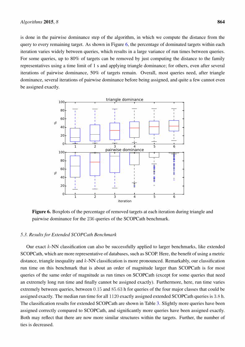
is done in the pairwise dominance step of the algorithm, in which we compute the distance from thequery to every remaining target. As shown in Figure 6, the percentage of dominated targets within eachiteration varies widely between queries, which results in a large variance of run times between queries.For some queries, up to 80% of targets can be removed by just computing the distance to the familyrepresentatives using a time limit of 1 s and applying triangle dominance; for others, even after severaliterations of pairwise dominance, 50% of targets remain. Overall, most queries need, after triangledominance, several iterations of pairwise dominance before being assigned, and quite a few cannot evenbe assigned exactly.

1 2 3 4 5 60

20

40

60

80

100

%

triangle dominance

1 2 3 4 5 6iteration

0

20

40

60

80

100

%

pairwise dominance

Figure 6. Boxplots of the percentage of removed targets at each iteration during triangle andpairwise dominance for the 236 queries of the SCOPCath benchmark.

5.3. Results for Extended SCOPCath Benchmark

Our exact k-NN classification can also be successfully applied to larger benchmarks, like extendedSCOPCath, which are more representative of databases, such as SCOP. Here, the benefit of using a metricdistance, triangle inequality and k-NN classification is more pronounced. Remarkably, our classificationrun time on this benchmark that is about an order of magnitude larger than SCOPCath is for mostqueries of the same order of magnitude as run times on SCOPCath (except for some queries that needan extremely long run time and finally cannot be assigned exactly). Furthermore, here, run time variesextremely between queries, between 0.15 and 85.63 h for queries of the four major classes that could beassigned exactly. The median run time for all 1120 exactly assigned extended SCOPCath queries is 3.8 h.The classification results for extended SCOPCath are shown in Table 3. Slightly more queries have beenassigned correctly compared to SCOPCath, and significantly more queries have been assigned exactly.Both may reflect that there are now more similar structures within the targets. Further, the number ofties is decreased.


Table 3. Classification results showing the number of queries out of the overall 1369 queriesthat have been assigned to a superfamily, the number of correct assignments, the number ofassignments computed exactly, thereof the number of correct classifications and the numberof ties that do not allow a superfamily assignment based on majority vote. The last two linesdisplay the number of correct assignments and ties for k-NN classification using TM-align.

k 10 9 8 7 6 5 4 3 2 1# correct 1303 1331 1334 1341 1341 1346 1344 1351 1348 1361# exact 1120 1182 1228 1271 1286 1339 1341 1352 1347 1368# exact and correct 1104 1166 1215 1257 1276 1329 1330 1341 1343 1360# ties 35 5 12 6 11 7 9 3 17 0# TM-align correct 1311 1347 1346 1350 1351 1354 1352 1353 1351 1361# TM-align ties 39 4 7 4 6 4 4 5 15 0

Figure 7 displays the progress of the computation. Here, many more target structures are removed bytriangle dominance and within the very first iteration of pairwise dominance compared to the SCOPCathbenchmark. For example, for most queries, more than 60% of targets are removed by triangle dominancealone. Only very few queries need to explicitly compute the distance to a large percentage of the targets,and almost 75% of queries can be assigned after only one round of pairwise dominance.

1 2 3 4 5 60

20

40

60

80

100

%

triangle dominance

1 2 3 4 5 6iteration

0

20

40

60

80

100

%

pairwise dominance

Figure 7. Boxplots of the percentage of removed targets at each iteration during triangle andpairwise dominance for the 1369 queries of the extended SCOPCath benchmark.


6. Discussion

The difficulty to optimally compute a superfamily assignment using k-NN increases with thedissimilarity of the k-th closest target and the query, because this target determines the dominationbound, and this bound becomes weaker when k increases. This can be observed in the different number ofexactly-assigned queries between SCOPCath and extended SCOPCath, on the one hand, and for differentk, on the other hand. Since SCOPCath has been filtered for low sequence identity, we can expect that thek-th neighbor is less similar to the query than the k-th neighbor in extended SCOPCath, and therefore, itis easier to compute extended SCOPCath exactly. Accordingly, the number of exactly-assigned queriestends to increase with decreasing k. In future work, we may use such properties of the distance boundsto decide which k is most appropriate for a given query.

Our exact classification is based on a well-known property of exact CMO computation: similarstructures are quick to align and are usually computed exactly, whereas dissimilar structures areextremely slow to align and usually not exactly. Therefore, we remove dissimilar structures early usingbounds. Distances between similar structures can then be computed (near-)optimal, and the resultingk-NN classification is exact.

Except for the case k = 1 on the extended benchmark, in terms of assignment accuracy, TM-alignperforms slightly better than max-CMO, and it usually has to some extent fewer ties. On the otherhand, both max-CMO and TM-align perform best in the case k = 1, and for that most relevant case,the two methods have the same accuracy. Considering that max-CMO is a metric and, thus, needsto compare structures globally, while TM-align is not, it still allows one to perform very accuratesuperfamily assignment.

While for the extended benchmark, max-CMO and TM-align have the same number of correctclassifications for the best choice of value for k, the somewhat better performance of TM-align in theother cases indicates that the max-CMO method could be further improved. A possible disadvantageof our metric is that it does not apply proper length normalization. For instance, if a protein structureis identical to a substructure of another protein, the corresponding max-CMO distance depends on thelength of the longer protein. For classification purposes, it would usually be better to rank a protein withsuch local similarity higher than another protein that is less similar, but of smaller length.

Moreover, although the current results suggest that, in terms of assignment accuracy, using only thenearest neighbor for classification works best, finding the k-nearest neighbor structures is still interestingand important. A new query structure is in need of being characterized, and the set of k closest structuresfrom a given classification gives a useful description on its location in structure space, especially if thisspace is metric. Note that, besides using the presented algorithm for determining the k-nearest neighbors,it could straightforwardly also be used to find all structures within a certain distance threshold of agiven query.

We show that our approach is beneficial for handling large datasets, the structures of which formclusters in some metric space, because it can quickly discard dissimilar structures using metric properties,such as triangle inequality. This way, the target dataset does not need to be reduced previously using adifferent distance measure, such as sequence similarity, which can lead to mistakes. Our classification isat all times based exclusively on structural distance.


Among the disadvantages of a heuristic approach for the task of large-scale structure classification,we can point to the observation that the obtained classifications are not stable. As versions of tools orrandom seeds change, the distance between structures may change, since the provable distance betweentwo structures is not known. With these distance changes, also the entire classification may change. Suchpossible, unpredictable changes in classification contradict the essential use of an automatic classificationas a reference. Furthermore, even if a given heuristic could be very fast, it always requires a pairwisenumber of comparisons for solving the classification problem by the k-NN approach. This requirementobviously becomes a notable hindrance with the natural and quick increase of the protein databases size.

7. Conclusion

In this work, we introduced a new distance based on the CMO measure and proved that it is atrue metric, which we call the max-CMO metric. We analyzed the potential of max-CMO for solvingthe k-NN problem efficiently and exactly and built on that basis a protein superfamily classificationalgorithm. Depending on the values of k, our accuracy varies between 89% for k = 10 and 95% for k = 1

for SCOPCath and between 95% and 99% for extended SCOPCath. The fact that the accuracy is highestfor k = 1 indicates that using more sophisticated rules than k-NN may produce even better results.

In summary, our approach provides a general solution to k-NN classification based on acomputationally-intractable measure for which upper and lower bounds are polynomially available. Byits application to a gold standard protein structure classification benchmark, we demonstrate that it cansuccessfully be applied for fully-automatic and reliable large-scale protein superfamily classification.One of the biggest advantages of our approach is that it permits one to describe the protein space in termsof clusters with their representative central structures, radii, intra-cluster and inter-clusters distances.Such a formal description is by itself a source of knowledge and a base for future analysis.

Acknowledgments

We are grateful to Noël Malod-Dognin and Nicola Yanev for discussions and useful suggestions and toSven Rahmann for providing computational infrastructure. We thank the reviewers for a careful readingand for the comments on this study.

Author Contributions

Rumen Andonov, Gunnar W. Klau, Mathilde Le Boudic-Jamin and Inken Wohlers conceived thek-NN classification approach using triangle bounds and the max-CMO metric. Rumen Andonov,Hristo Djidjev and Gunnar W. Klau proved that max-CMO is a metric and other previously usedmeasures not. Inken Wohlers implemented the classification algorithm. Mathilde Le Boudic-Jamin andInken Wohlers conducted the computational experiments and prepared the results. The authors jointlyexamined the results and wrote the paper.

Conflicts of Interest

The authors declare no conflict of interest.


References

1. Murzin, A.G.; Brenner, S.E.; Hubbard, T.; Chothia, C. SCOP: A structural classification ofproteins database for the investigation of sequences and structures. J. Mol. Biol. 1995,247, 536–540.

2. Orengo, C.A.; Michie, A.D.; Jones, S.; Jones, D.T.; Swindells, M.B.; Thornton, J.M. CATH—Ahierarchic classification of protein domain structures. Structure 1997, 5, 1093–1108.

3. Bernstein, F.; Koetzle, T.; Williams, G.; Meyer, E.M., Jr.; Brice, M.; Rodgers, J.; Kennard, O.;Shimanouchi, T.; Tasumi, M. The protein data bank: A computer-based archival file formacromolecular structures. Arch. Biochem. Biophys. 1978, 185, 584–591.

4. Godzik, A.; Skolnick, J.; Kolinski, A. Regularities in interaction patterns of globular proteins.Protein Eng. 1993, 6, 801–810.

5. Caprara, A.; Carr, R.; Istrail, S.; Lancia, G.; Walenz, B. 1001 optimal PDB structure alignments:Integer programming methods for finding the maximum contact map overlap. J. Comput. Biol.2004, 11, 27–52.

6. Xie, W.; Sahinidis, N.V. A reduction-based exact algorithm for the contact map overlap problem.J. Comput. Biol. 2007, 14, 637–654.

7. Pelta, D.A.; González, J.R.; Vega, M.M. A simple and fast heuristic for protein structurecomparison. BMC Bioinform. 2008, 9, 161.

8. Andonov, R.; Malod-Dognin, N.; Yanev, N. Maximum contact map overlap revisited. J. Comput.Biol. 2011, 18, 27–41.

9. Malod-Dognin, N.; Boudic-Jamin, M.L.; Kamath, P.; Andonov, R. Using dominances for solvingthe protein family identification problem. In Algorithms in Bioinformatics; Springer: Berlin,Germany, 2011; pp. 201–212.

10. Wohlers, I.; Malod-Dognin, N.; Andonov, R.; Klau, G.W. CSA: Comprehensive comparison ofpairwise protein structure alignments. Nucleic Acids Res. 2012, 40, W303–W309.

11. Malod-Dognin, N.; Przulj, N. GR-Align: Fast and flexible alignment of protein 3D structuresusing graphlet degree similarity. Bioinformatics 2014, 30, 1259–1265.

12. Clarkson, K.L. Nearest-neighbor searching and metric space dimensions.Nearest-Neighbor Methods for Learning and Vision: Theory and Practice; MIT Press:Cambridge, MA, USA, 2006.

13. Moreno-Seco, F.; Mico, L.; Oncina, J. A modification of the LAESA algorithm for approximatedk-NN classification. Pattern Recognit. Lett. 2003, 24, 47–53.

14. Mico, M.L.; Oncina, J.; Vidal, E. A new version of the nearest-neighbour approximating andeliminating search algorithm (AESA) with linear preprocessing time and memory requirements.Pattern Recognit. Lett. 1994, 15, 9–17.

15. Rogen, P.; Fain, B. Automatic classification of protein structure by using Gauss integrals. Proc.Natl. Acad. Sci. 2003, 100, 119–124.

16. Harder, T.; Borg, M.; Boomsma, W.; Røgen, P.; Hamelryck, T. Fast large-scale clustering ofprotein structures using Gauss integrals. Bioinformatics 2012, 28, 510–515.


17. Zhang, Y.; Skolnick, J. TM-align: A protein structure alignment algorithm based on theTM-score. Nucleic Acids Res. 2005, 33, 2302–2309.

18. Lathrop, R.H. The protein threading problem with sequence amino acid interaction preferencesis NP-complete. Protein Eng. 1994, 7, 1059–1068.

19. Horadam, K.; Nyblom, M. Distances between sets based on set commonality. Discret. Appl.Math. 2014, 167, 310–314.

20. Altman, N.S. An introduction to kernel and nearest-neighbor nonparametric regression. Am.Stat. 1992, 46, 175–185.

21. Mavridis, L.; Venkatraman, V.; Ritchie, D.W.; Morikawa, N.; Andonov, R.; Cornu, A.;Malod-Dognin, N.; Nicolas, J.; Temerinac-Ott, M.; Reisert, M.; et al. SHREC’10 Track: ProteinModel Classification; The Eurographics Association: Norrköping, Sweden, 2010.

22. Csaba, G.; Birzele, F.; Zimmer, R. Systematic comparison of SCOP and CATH: A new goldstandard for protein structure analysis. BMC Struct. Biol. 2009, 9, 23.

23. Wohlers, I.; Domingues, F.S.; Klau, G.W. Towards optimal alignment of protein structuredistance matrices. Bioinformatics 2010, 26, 2273–2280.

24. Wang, S.; Ma, J.; Peng, J.; Xu, J. Protein structure alignment beyond spatial proximity. Sci. Rep.2013, 3, 1448.

c© 2015 by the authors; licensee MDPI, Basel, Switzerland. This article is an open access articledistributed under the terms and conditions of the Creative Commons Attribution license(http://creativecommons.org/licenses/by/4.0/).

automatic classification of protein structures using the ... · automatic classification of protein...

Documents